Evaluation of wireline well logs from the borehole ...

Óluva EllingsgaardExamensarbeten i Geologi vidLunds universitet - Berggrundsgeologi, nr. 212

Geologiska institutionenCentrum för GeoBiosfärsvetenskap

Lunds universitet2007

Evaluation of wireline well logs fromthe borehole Kyrkheddinge-4 bycomparsion to measured coredata

Evaluation of wireline well logs from the borehole Kyrkheddinge-4 by

comparison to measured core data

Bachelor Thesis Óluva Ellingsgaard

Department of Geology Lund University

2007

Table of Contents

1. Introduction and project outline ...................................................................................................................... 5 2. Main geology of southwest Skåne..................................................................................................................... 6 2.1 Geological structures of the Kyrkheddinge area 6 2.2 Sedimentary sequence of Well Kyrkheddinge-4 6 3. Material and Methods....................................................................................................................................... 6 3.1 Chemical Analysis 7 3.2 Description and usability of the logs used 7 3.2.1 Caliper log 7 3.2.2 Resistivity log 7 3.2.3 Spontaneous Potential log 7 3.2.4 Gamma Ray log 7 3.2.5 Density log 8 3.2.6 Neutron log 9 3.2.7 Sonic log 9 4. Formation analysis ............................................................................................................................................ 9 4.1 Porosity values derived from the Density, Neutron and Sonic logs 9 4.2 Corrections 11 5. Results and interpretation .............................................................................................................................. 11 5.1 Evaluation of well log calculated porosity to measured porosities from core data 15 5.1.1 Formation factor and water saturation 15 5.2 Permeability 15 5.3 Possible sources of error and quality of data 17 6. Discussion ......................................................................................................................................................... 17 7. Conclusions ...................................................................................................................................................... 19 8. Acknowledgements .......................................................................................................................................... 19 9 References ........................................................................................................................................................ 20 Appendix I: Table with the 41 derived values from the wireline logs 21 Appendix II: The permeability measured from core values versus the calculated permeability values 22

Cover Picture: Wireline logging.

Evaluation of wire-line well logs from the borehole Kyrkhed-dinge-4 by comparison to measured core data Óluva Ellingsgaard

Ellingsgaard, Ó.,2007. Evaluation of wire-line well logs from the borehole Kyrkheddinge-4 by comparison to measured core data. Exam in Geology at Lunds University. No 212, 22pp, 15 ECTS points.

Keywords: Kyrkheddinge, wire-line, well logs, porosity, permeability, Lund Member

Óluva Ellingsgaard, Department of geology, GeoBiosphere Science centre, Lund University, Sölvegatan 12, SE-22362 Lund, Sweden. E-mail: [email protected]

Abstract: This study is an evaluation of formation characteristics, as derived from wire-line well logs, of the Lund Member in the borehole Kyrkheddinge-4, 3 km east of Staffanstorp, Skåne, Sweden, through the comparison to measured core data. The purpose is to assess the feasibility of using some of the porosity and permeability equa-tions and cross-plots derived for the investigated section and applying them to deeper aquifer formations in Kyrk-heddinge-4, where no core data exist.

Shale corrected porosities are calculated from the Density, Neutron and Sonic logs for 41 levels from the borehole, including additional porosities from the compaction corrected Sonic log. These porosities were derived using stan-dard equations and cross-plots. These data were compared to porosity values obtained directly from core samples from the same investigated levels. The results suggested that the shale corrected Density log values have the strong-est linear relationships to the measured core data, although the R2 value is extremely low at 0.29. However, the R2 value increases to 0.74 for sandstone samples, although this is based on 4 data points, which compares to an R2 value of 0.12 for the 26 marlstone samples.

The results suggest it is not possible to fully rely upon the porosity values obtained from the wireline log equations. The main reason is due to the complex lithologies and the high amount of shale/clay present in the formations. To-gether with shale data, lithological characteristics such as compaction of the sandstones are important, to obtain accurate corrected porosity values on which the equations and cross-plots are based. Permeabilities were unable to be calculated and therefore, unable to be compared to the measured core permeabilities. This was due to the lack of data of the irreducible water saturation (Swirr) parameter, which cannot be obtained in Kyrkheddinge-4, as the per-meable horizons are 100% water saturated and the equations required to calculate Swirr principally rely upon the presence of hydrocarbons.

Utvärdering av borrhålsloggar från borrhålet Kyrkheddinge-4 genom en jämförelse med uppmätta kärndata

Óluva Ellingsgaard

Ellingsgaard, Ó. 2007: Utvärdering av borrhålsloggar från borrhålet Kyrkheddinge-4 genom en jämförelse med uppmätta kärndata. Examensarbete i geologi från Lunds University. Nr. 212, 22s, 10 points.

Nyckelord: Kyrkheddinge, borrhålsloggar, porositet, permeabilitet, Lund Member

Óluva Ellingsgaard, Geologiska institutionen, Centrum för GeoBiosfärsvetenskap (CGB) vid Lund University, Söl-vegatan 12, SE-22362 Lund, Sverige. E-mail: [email protected]

Sammanfattning: Denna studie är en utvärdering av borrhålsloggar från borrhålet Kyrkheddinge-4, beläget 3 km öster om Staffanstorp, Skåne, särskilt vad gäller formationsegenskaperna i borrhålets undre delar, d.v.s. i Lunda-sandstenen (Lund Member). Syftet har varit att undersöka hur porositets- och permeabilitetsvärden beräknade med hjälp av standardekvationer och krossplottar förhåller sig till uppmätta värden från några kärntagna avsnitt och hur pass tillförlitliga reservoirdata beräknade från borrhålsloggar kan vara i de understa vattenförande nivåerna i Kyrk-heddinge-4, där kärndata saknas.

Lerkorrigerade porositetsvärden har beräknats från densitets-, neutron- och sonicloggarna för 41 nivåer i borrhålet och dessutom har kompaktionskorrigering utförts på sonicloggen. Porositetsvärdena har erhållits genom använd-ning av standardekvationer och krossplottar. De har sedan jämförts med värden erhållna från borrkärnor tagna från flera nivåer av de understa 500 m av borrhålet. Resultaten visar att porositeten beräknade från de lerkorrigerade densitetsvärdena stämmer bäst överens med uppmätta kärndata, även om R2 är extremt lågt på bara 0,29. R2 höjs dock till 0,74 för sandstensnivåerna, men är då baserat på enbart 4 sandstensnivåer, jämfört med ett R2 på 0,12 för de 26 märgelstensnivåerna.

Resultaten antyder att porositetsvärden beräknade utifrån data från borrhålsloggarna är mindre tillförlitliga. Detta torde bero på såväl litologiska egenskaper som den höga halten av ler i formationen. Tillsammans med lerinnehållet är kunskapen om sandstenarnas kompaktionsegenskaper viktiga för att erhålla goda porositetsvärden. Godtagbara permabilitetsvärden kunde inte beräknas utifrån de befintliga borrhålsloggarna och därför blev en jämförelse med de uppmätta permeabilitetsvärdena från kärnorna inte möjlig. Detta beror på att det inte var möjligt att beräkna Swirr (irreducible water saturation) parametern, då de permeabla horisonterna är 100% vattenförande, medan befintliga permeabilitetsekvationer bygger på att en viss del kolväten finns i formationen.

5

1. Introduction and project out-line

During the years 1976 to 1982 the Geological Survey of Sweden (SGU) carried out geological and geophysi-cal investigations in the Kyrkheddinge area, 3 km E of Staffanstorp in Skåne, Sweden (Fig. 1). The aim of these investigations was to find potential sites for aqui-fer storage of natural gas. The next step was to deter-mine the technical and economic feasibility of this project. This survey was initiated in early 1983 with Swedegas AB as the prime investigator. They started by shooting four seismic profiles in order to map the structures of the rock strata and subsequently, four wells were drilled (Figs. 2 & 3). The fourth well, Kyrkheddinge-4, was drilled to establish the presence and properties of the potential Campanian sandstone storage reservoir, referred to as the Lund Member

(Erlström 1994). Pipeline Engineering (PLE) produced a core investigation report based on eight cores taken from eight different levels from well Kyrkheddinge-4 (Hagconsult 1983). This study begins by describing the extension of the Lund Member and the main geology of the Kyrkheddinge area. Material and methods used will be presented followed by a formation analysis in Kyrk-hedding-4. Then the results will be presented and the study concludes with a discussion and evaluation of the usefulness of wireline logs in this kind of rock strata, by comparing the porosity values enhanced from calculations during the formation analysis, with the measured porosity values from core investigations. In short, this studies outline is a quality check of the usability of wireline logs in aquifer formations where no hydrocarbons are present and where the de-gree of consolidation of the reservoir sequences is low.

Fig. 1. a) Geolo-gical map over Skåne, the loca-tion of well site Kyrkheddinge-4 is higlighted. b) Cro s s - sec t io n over Skåne and l o c a t i o n o f Kyrkheddinge (Fredén 2002).

a

b

6

2. Main geology of southwest Skåne

Within the Fennoscandian Border Zone, the border zone between the Fennoscandian shield in the north and the Danish-Polish embayment in the south, several horsts are located, one being the Romleåsen horst (Fig. 1). The area southwest of Romelåsen is depressed in relation to the horst, where the general dip directions changes from NE to SW moving in a southwesterly direction away from the horst. In SW Skåne the base-ment is partly overlain by 800 meters of Cambro-Silurian strata. This is overlain by various sedimentary strata from the Triassic to the Palaeogene. These strata

are dominated by those of the Upper Cretaceous with an average thickness of about 1200 m. This includes the Campanian sandstone sequence, i.e. the Lund Member, which is up to 800 m thick. The Lund Mem-ber probably covers the whole area SW of Romelåsen and was deposited during a period of tectonic activity along the border zone (Anderson 1984). 2.1 Geological structures of the Kyrkhed-

dinge area Both the depth converted section of seismic line S4 and the two way transit time map from Kyrkheddinge (Figs. 2 & 3) show that there is an anticlinal structure in the area. From the depth converted S4 section (Fig. 2) it is possible to see that the anticline is transected to the north by two faults, α and β, respectively. These faults were later proved not to interfere with the poten-tial storage strata (Hagconsult 1983). 2.2 Sedimentary sequence of Well Kyrk-

heddinge-4 The sedimentary sequence of the area starts with Qua-ternary deposits that are about 32 m thick. The se-quence from a depth of 32 to 55 m were not recovered, but are presumable of Palaeogene age, i.e. Danian limestone. Between the depths of 55 to 178 m Maas-trichtian chalk was encountered. From the base of the chalk to a depth of 402 m there is a rapid change in lithology from chalk into fine limestone and claystone. Claystone contents vary between 20-40% between 55-280 m and 50-70% between 280-402 m. From 402 m to the base of the well (total depth (TD) of 830 m), the potential storage level, there are sandstones alternating with sandy claystone/limestone of the Lund Member. The grain size varies from medium-coarse grained sand in the upper parts to fine-medium grained sand in the lower parts. The sandstones are mostly unconsoli-dated and poorly cemented, but in-between there are also thin, hard, well-cemented layers commonly re-ferred to as caprocks (Hagconsult 1983). Consequently, the lower parts of the formation have been divided into caprock and reservoir units for explorational reasons (Fig. 5).

3. Material and methods The data used in this study are primarily obtained from the reports and well logs (Fig. 5 & Appendix I) pro-duced in connection with the work done by Swedegas AB and others in the Kyrkheddinge area. Unfortu-nately, individual logs were unable to be examined and information was obtained directly from composite logs and therefore, the quality of these logs as well as the data derived from them has to be taken into considera-tion. To support the analysis of the well logs, Schlum-bergers Log Interpretation volumes I and II and the accompanying interpretation charts were consulted. After deriving values from the composite logs, a variety of calculations were performed and cross-plots used to get the most reliable porosity and perme-

Fig. 2. A deep converted section of seismic line S4 in Kyrk-heddinge and placement of the four wells (Hagconsult 1983).

Fig. 3. A time contour map expressed in two way time over the Kyrkheddinge area. Seismic line S4 is highlighted as well as the well side of Kyrkhedding-4 ( Hagkonsult 1983).

α

β

7

ability values for later comparisons with measured data obtained directly from core analyses. 3.1 Chemical analysis In order to determine water saturation values the water resistivity (Rw) of the investigated formations had to be obtained. There are different methods that can be used to obtain this, e.g. the Spontaneous Potential (SP) log curve or directly from chemical analysis. Due to the poor resolution of the SP curve and because of the possibility of obtaining the Rw from chemical analysis, the latter method was used as comprehensive chemical data are available for the investigated formations (SGAB 1983, Schlumberger 1972 & 1979). 3.2 Description and usability of the logs

used In Kyrkheddinge-4, wireline logging was carried out by Swedegas AB from the top to a depth of 500 m and by Schlumberger from 515 meters to TD of 830 m. The latter log suites by Schlumberger are used in this study. Wireline logs allow for various calculation pos-sibilities and they can give many different parameters. For this study, only seven of the many possible logs were used. They include the Caliper, Resistivity, Spontaneous Potential, Gamma Ray, Density, Neutron and Sonic logs. These seven different logs are briefly described below, in terms of how they work and what primary usage they have. 3.2.1 Caliper log The Caliper log measures the diameter in the borehole for each specific level and is therefore useful to detect washouts. Washouts occur when the formation is loose or unconsolidated and the drilling mud flushes away parts of the formation. The drilling mud is a fluid that lubricates and cools the drill-bit and flushes cuttings to the surface, which can be examined to determine the lithology of the drilled sequence. The mud can also invade the formation to various depths depending on the consolidation of the unit, which can therefore, af-fect the formations physical properties and needs to be taken into account. The curve used in this study ranges between 10 and 20 inches (i.e. 25 to 50 cm) and values derived from the curve have to be added to the diameter of the borehole which was 97/8 inches (e.g. about 25 cm) (Cherns et al. 1983). The Caliper logs are essential for the interpreta-tion of other logs whose responses are sensitive to the state of the borehole (PLE 83a). 3.2.2 Resistivity log The Resistivity log measures the electrical resistivity of the formation. It is possible to get three different resistivity values from the formation: deep resistivity, medium resistivity and spherically focused resistivity (shallow resistivity) (PLE 83a). In this study the deep resistivity log was used as it is most likely to give the

best true resistivity values of the sections where the drilling mud did not infiltrate the formation. To meas-ure the resistivity, currents are passed through the for-mation between electrodes and the voltage drop is measured and the resistivity calculated. The unit of measure for resistivity is the ohmm or ohm-meter2/meter (Schlumberger 1972).

3.2.3. Spontaneous Potential (SP) log The Spontaneous Potential (SP) log records naturally occurring (static) electrical potential in the Earth. It shows the difference between the potential of a mov-able electrode in the borehole and the fixed potential of an electrode at the surface (Schlumberger 1972). The most useful component of this difference is the electrochemical potential since it can cause a signifi-cant deflection on opposite sides of permeable beds. The magnitude of the deflection depends mainly on the salinity contrast between drilling mud and forma-tion water, and the clay content of the permeable bed. The SP curve is therefore used to detect permeable beds and to estimate formation water salinity and for-mation clay content. The unit for the SP curve is in millivolt, mV, and in this study it has been used for shale (clay) correct ion of the porosi ty logs (Schlumberger 1972).

3.2.4 Gamma Ray (GR) log The Gamma Ray (GR) log measures true natural ra-dioactivity of the formations, on the basis of spectro-metric analysis of the three natural gamma ray emit-ting elements: Potassium40 (K40), Thorium232 (Th232) and Uranium238 (U238). The GR log is useful because of the different gamma ray signatures for shale (including claystones) and sandstone, as the radioac-tive elements tend to concentrate in clay and shale. Clean formations usually show low values of radioac-tivity. The unit for the GR is expressed in American Petroleum Institute (API) units, and it is often used as

Fig. 4. The Compen-sated Density Sonde. The figure shows how the sonde is attached to the well hole wall by a spring and explains why washouts make re-cordings uncertain (from Schlumberger 1972).

8

a substitute for the SP curve in holes where the SP is unsatisfactory or when the borehole has been cased (Schlumberger 1972). Low GR readings are associated with sandstones, while claystones/shales emit higher readings.

3.2.5 Density log The Density log responds to the electron density of the material in the formation. A radioactive source emits medium-energy gamma rays into the formation; these gamma rays travel at high speed and collide with elec-trons in the formation. At each collision the gamma ray looses some energy. When it comes back to the

detector it responds to this phenomena and measures the energy left in the gamma rays which gives an indi-cation of formation density. The interaction is called Compton scattering. The unit for the density is g/cm3. The Density log is useful for porosity determinations, because the number of Compton is related to the num-ber of electrons in the formation, and the response of the Density tool is determined essentially by the elec-tron density (the number of electrons per cubic centi-metre) in the formation. Electron density is related to the true bulk density (ρb) which in turn depends on the formation porosity (Schlumberger 72). Due to the way the Density log is attached by a spring to the borehole wall (Fig. 4), it is sensitive to

Fig. 5. This figure shows stratigraphy, depth, horizons and caprocks of the borehole Kyrkheddinge-4. Additionally the GR, the SP, the Caliper and the three porosity logs; the Sonic, Density and Neutron logs are presented. The GRmax and the SSP as well as the first and last levels derived are highlighted. The four levels, 27-30 used in the dissussion are also highlighted (Hagconsult 1983 & PLE 1983a).

9

washouts. The sonde radiates to a certain distance and records therefore not in the formation but in the wash-out. 3.2.6 Neutron log The Neutron log works similarly to the Density log. High-speed neutrons are emitted from a source, which reacts principally with any hydrogen in the formation generating gamma rays that are measured by the detec-tor. Hydrogen is primarily contained within water or hydrocarbons, but also hydrated minerals but this can be accounted for. Thus, the Neutron log is a used tool for indicating formation porosity and can also distin-guish between gas, which produces a lower response, compared to oil or water. The Neutron curve is meas-ured as a percentage, known as “Limestone porosity” (Schlumberger 1972:49). The Neutron log is as the Density log attached by a spring to the borehole wall (Fig. 4), and therefore sensitive to washouts because the sonde radiates to a certain distance and records therefore not in the formation, but in the washout.

3.2.7 Sonic log The Sonic log is an acoustic tool that displays the in-terval travel time, ∆t, the amount of time for a com-pressional sound wave to travel a certain distance and is proportional to the reciprocal of velocity. The tool emits a sound wave that travels from the source to the formation and back to the receiver. The interval travel time is dependant on the lithology and porosity of the formation and this makes the Sonic logging a very useful tool when it comes to determining porosity. The unit for the Sonic log is microseconds per metre (µs/m) (Schlumberger 1972). 4. Formation analysis Formation evaluation or analysis of well Kyrkhed-dinge-4 has been performed at levels where cores have been obtained and investigated in the laboratory for porosity and permeability, see appendix I. This was necessary for comparison between the log interpreta-tions and the measured data from the core investiga-tions. Log values have been read at 50 cm intervals which gave 41 values through the examined section that can be compared directly to values obtained from core samples (Appendix I & Fig. 5). Due to the uncon-solidated nature of the sandstones it was difficult to obtain satisfactory core samples for the investigation and consequently only 4 samples are sandstones and the remaining 32 samples are predominantly marl-stones. In addition, 5 of the samples have been inter-preted as potential aquifers and 31 samples have been classified as caprocks (Appendix I & Fig. 5).

4.1 Porosity values from the Density, Neutron and Sonic logs

To obtain the best possible porosity values from the Density and Sonic logs, equations and cross-plot meth-

ods are used. Lithology corrections were made to the Neutron log derived values (фN), in order to obtain true porosity values as the log is expressed in “Limestone Porosity” units and this was accomplished by using Schlumberger chart Por-13 (Schlumberger 1979). The equations used to get porosity values from the Density (фD) and Sonic (фS) logs were:

фD = ρma-ρb/ρma-ρf and фS = ∆t-∆tma/∆tf-∆tma

(Schlumberger 1972) where ρma is the density of the rock matrix, ρb is the bulk density value derived from the Density log and ρf is the density of the rock fluid. For the Sonic equation, ∆t, is the interval transit time, the number derived from the Sonic log. The ∆tma is the transit time in the rock matrix and ∆tf is the transit time in the rock fluid. Apart from ρb and the ∆t, which are derived from the logs (Appendix I), the other figures needed in the equations, (and depend respectively on matrix and fluid), have been derived from Schlumberger 1979. The 41 porosity values, from the Neutron correction chart (фN) and the equations for the Density (фD) and Sonic log (фS), are presented in Table 1.

Fig. 6. The figure shows where the analysed points lay within the M-N plot, the red scattered dots. Because there has not been any anhydrite minerals proved in the formation, the figure shows very clearly that the levels are all within the approxi-mate shale region (Schlumberger 1979).

10

Table 1.

ΦN Porosity from the Neutron log ΦD Porosity from the Density log Φs Porosity from the Sonic log From corr. Chart Φ = ρma-ρb/ρma-ρf Φ = ∆t-∆tma/∆tf-∆tma No % % % 1 23 21.9 38.6 2 34.1 21.9 52.8 3 31.9 16.1 55 4 23 13.7 30.9 5 27.1 13 34 6 29.6 14.3 36.5 7 27.1 15.5 33.3 8 29.6 16.1 37.4 9 28 14.3 34.9 10 24.3 14.3 29.8 11 28 24.2 39 12 23.2 17.7 33.2 13 35.5 18 50.6 14 29.5 21.7 40.9 15 33.6 26.1 51.6 16 24.5 28.6 40.6 17 32 33.5 58.7 18 32 14.9 48.1 19 29.5 24.2 41.1 20 31.5 33.5 53.9 21 33.2 18 54.5 22 19 13.7 34 23 21.5 13.5 26.6 24 21.3 15.5 30.5 25 30.2 28.6 36.4 26 26.1 21.3 31.5 27 24.2 24.5 25.3 28 29 16.1 37.9 29 31 20.5 40.9 30 37.3 20.5 40.5 31 22.3 9 20.5 32 28 12.4 35.6 33 25.5 14.3 40.2 34 25.5 13.7 37 35 29 17.4 38.4 36 25.5 16.8 33 37 28.3 18 37.2 38 23.2 17.4 37.4 39 33.4 20.5 37.6 40 20 13 26.5 41 26.1 16.1 37.4

11

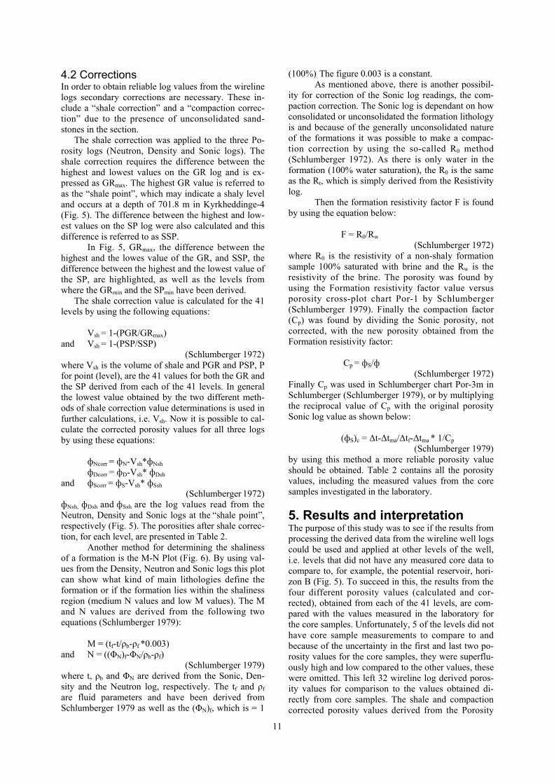
4.2 Corrections In order to obtain reliable log values from the wireline logs secondary corrections are necessary. These in-clude a “shale correction” and a “compaction correc-tion” due to the presence of unconsolidated sand-stones in the section.

The shale correction was applied to the three Po-rosity logs (Neutron, Density and Sonic logs). The shale correction requires the difference between the highest and lowest values on the GR log and is ex-pressed as GRmax. The highest GR value is referred to as the “shale point”, which may indicate a shaly level and occurs at a depth of 701.8 m in Kyrkheddinge-4 (Fig. 5). The difference between the highest and low-est values on the SP log were also calculated and this difference is referred to as SSP. In Fig. 5, GRmax, the difference between the highest and the lowes value of the GR, and SSP, the difference between the highest and the lowest value of the SP, are highlighted, as well as the levels from where the GRmin and the SPmin have been derived.

The shale correction value is calculated for the 41 levels by using the following equations: Vsh = 1-(PGR/GRmax) and Vsh = 1-(PSP/SSP)

(Schlumberger 1972) where Vsh is the volume of shale and PGR and PSP, P for point (level), are the 41 values for both the GR and the SP derived from each of the 41 levels. In general the lowest value obtained by the two different meth-ods of shale correction value determinations is used in further calculations, i.e. Vsh. Now it is possible to cal-culate the corrected porosity values for all three logs by using these equations: фNcorr = фN-Vsh*фNsh фDcorr = фD-Vsh* фDsh and фScorr = фS-Vsh* фSsh

(Schlumberger 1972) фNsh, фDsh and фSsh are the log values read from the Neutron, Density and Sonic logs at the “shale point”, respectively (Fig. 5). The porosities after shale correc-tion, for each level, are presented in Table 2. Another method for determining the shaliness of a formation is the M-N Plot (Fig. 6). By using val-ues from the Density, Neutron and Sonic logs this plot can show what kind of main lithologies define the formation or if the formation lies within the shaliness region (medium N values and low M values). The M and N values are derived from the following two equations (Schlumberger 1979): M = (tf-t/ρb-ρf *0.003) and N = ((ΦN)f-ΦN/ρb-ρf)

(Schlumberger 1979) where t, ρb and ΦN are derived from the Sonic, Den-sity and the Neutron log, respectively. The tf and ρf are fluid parameters and have been derived from Schlumberger 1979 as well as the (ΦN)f, which is = 1

(100%). The figure 0.003 is a constant. As mentioned above, there is another possibil-ity for correction of the Sonic log readings, the com-paction correction. The Sonic log is dependant on how consolidated or unconsolidated the formation lithology is and because of the generally unconsolidated nature of the formations it was possible to make a compac-tion correction by using the so-called R0 method (Schlumberger 1972). As there is only water in the formation (100% water saturation), the R0 is the same as the Rt, which is simply derived from the Resistivity log. Then the formation resistivity factor F is found by using the equation below: F = R0/Rw

(Schlumberger 1972) where R0 is the resistivity of a non-shaly formation sample 100% saturated with brine and the Rw is the resistivity of the brine. The porosity was found by using the Formation resistivity factor value versus porosity cross-plot chart Por-1 by Schlumberger (Schlumberger 1979). Finally the compaction factor (Cp) was found by dividing the Sonic porosity, not corrected, with the new porosity obtained from the Formation resistivity factor: Cp = фS/ф

(Schlumberger 1972) Finally Cp was used in Schlumberger chart Por-3m in Schlumberger (Schlumberger 1979), or by multiplying the reciprocal value of Cp with the original porosity Sonic log value as shown below: (фS)c = ∆t-∆tma/∆tf-∆tma * 1/Cp

(Schlumberger 1979) by using this method a more reliable porosity value should be obtained. Table 2 contains all the porosity values, including the measured values from the core samples investigated in the laboratory.

5. Results and interpretation The purpose of this study was to see if the results from processing the derived data from the wireline well logs could be used and applied at other levels of the well, i.e. levels that did not have any measured core data to compare to, for example, the potential reservoir, hori-zon B (Fig. 5). To succeed in this, the results from the four different porosity values (calculated and cor-rected), obtained from each of the 41 levels, are com-pared with the values measured in the laboratory for the core samples. Unfortunately, 5 of the levels did not have core sample measurements to compare to and because of the uncertainty in the first and last two po-rosity values for the core samples, they were superflu-ously high and low compared to the other values, these were omitted. This left 32 wireline log derived poros-ity values for comparison to the values obtained di-rectly from core samples. The shale and compaction corrected porosity values derived from the Porosity

12

Table 2.

ΦNcorr from shale ΦDcorr from shale ΦScorr from shale

ΦScorr from compaction ΦCore

No ΦNcorr= ΦN-Vsh*ΦNsh ΦDcorr= ΦD-Vsh*ΦDsh ΦScorr = ΦS-Vsh*ΦSsh (фS)c= ∆t-∆tma/∆tf-∆tma*1/Cp Measured

% % % % % 1 22.5 21.6 37.9 29.7 3.5 2 25.2 16.1 40.4 31.1 11.0 3 18.9 7.7 36.9 28.9 15.0 4 15.3 8.7 20.1 22.1 5.0 5 17.5 6.8 20.7 16.2 14.0 6 19.3 7.6 22.2 14.6 19.0 7 15.9 8.2 17.7 15.9 18.5 8 17.6 8.3 20.8 16.3 17.5 9 16.8 7.0 19.3 17.5 10.5 10 13.5 7.3 14.9 18.6 18.5 11 16.8 16.9 23.4 21.5 20.5 12 10.8 9.6 15.9 22.0 17.0 13 20.3 8.1 29.5 21.5 7.0 14 14.9 12.2 20.6 22.0 15.0 15 22.1 18.7 35.7 26.1 16 22.4 27.2 37.7 30.1 17 26.8 30.2 51.5 29.9 20.0 18 28.7 12.8 43.6 27.0 11.0 19 26.2 22.1 36.6 27.0 22.5 20 23.9 28.6 43.3 31.0 21 23.2 11.5 40.7 27.0 23.0 22 8.4 6.9 19.4 20.5 15.0 23 12.8 7.9 14.6 20.9 24 12.6 9.9 18.4 21.8 15.0 25 25.6 25.6 30.0 24.3 25.0 26 22.3 18.8 26.2 27.4 28.0 27 18.1 20.6 16.8 28.1 23.0 28 17.5 8.7 22.0 25.0 11.5 29 15.7 10.6 19.6 22.0 23.0 30 14.3 12.1 22.4 20.5 23.5 31 10.8 1.6 4.6 18.1 13.0 32 15.6 4.3 18.3 17.5 19.0 33 12.6 5.9 22.3 17.0 11.5 34 11.4 4.6 17.5 17.0 15.0 35 16.3 9.2 20.8 17.0 11.5 36 11.9 8.0 14.1 17.0 17.0 37 15.3 9.6 19.1 17.9 19.5 38 7.9 7.5 16.1 18.3 20.0 39 21.9 13.1 21.7 18.9 7.5 40 11.6 7.5 14.8 17.3 14.0 41 13.4 7.9 19.8 16.9

13

Fig. 7. The figure shows the measured core porosity values versus the four different corrected porosity values ob-tained from the logs. The strongest correlations have a R2 value closest to 1.

a b

c d

Comparsion of porosity values

R2 = 0.2901

0.0

5.0

10.0

15.0

20.0

25.0

30.0

35.0

0.0 10.0 20.0 30.0

Measured core porosity (%)

Poro

sity

from

the

shal

e co

rrec

ted

Den

sity

log

(%) R2 = 0.0506

0.0

5.0

10.0

15.0

20.0

25.0

30.0

35.0

0.0 10.0 20.0 30.0


Poro

sity

from

the

shal

e co

rrec

ted

Neu

tron

log

(%)

R2 = 0.0182

0.0

10.0

20.0

30.0

40.0

50.0

60.0

0.0 20.0 40.0 60.0


Poro

sity

from

the

shal

e co

rrec

ted

Soni

c lo

g (%

) R2 = 0.0733

0.0

5.0

10.0

15.0

20.0

25.0

30.0

35.0

0.0 10.0 20.0 30.0


Poro

sity

from

the

com

pact

ion

corr

ecte

d So

nic

log

(%)

14

Fig. 8. This figure shows the same comparisons as Fig. 7 but here the two lithologies sandstone and marlstone are separated. This gives a better view over which equations give the best correlations because the equations are dependent on the lithology. The highest R2 (i.e. closest to 1) signifies a strong linear relationship (i.e. strong correlation).

Comparsion of porosity values for different lithologies

a b

c d

R2 = 0,0027 for marlstoneR2 = 0,5701 for sandstone

0.0

5.0

10.0

15.0

20.0

25.0

30.0

35.0

0.0 10.0 20.0 30.0


Poro

sity

from

the

shal

e co

rrec

ted

Neu

tron

log

(%)

M arlstoneSandstoneM ixtures sst/marlstone and limestone/marlstoneLinjär (M arlstone)Linjär (Sandstone)


0.0

5.0

10.0

15.0

20.0

25.0

30.0

35.0

0.0 10.0 20.0 30.0


Poro

sity

from

the

shal

e co

rrec

ted

Den

sity

log

(%)



0.0

10.0

20.0

30.0

40.0

50.0

60.0

0.0 20.0 40.0 60.0


Poro

sity

from

the

shal

e co

rrec

ted

Soni

c lo

g (%

)



0.0

5.0

10.0

15.0

20.0

25.0

30.0

35.0

0.0 10.0 20.0 30.0


Poro

sity

from

the

com

pact

ion

corr

ecte

d So

nic

log

(%)


15

logs are compared to the porosity values derived from the core samples in Figs. 7 and 8.

5.1 Evaluation of well log calculated po-

rosity to measured porosity from core data

As shown in Fig. 7, the correlation between the four different porosity values obtained from calculations on the wireline data with the measured core values are very different. The R2 value is a statistical method of evaluating the linear relationship between two vari-ables, where values close to 1 show a strong correla-tion, (conversely, the lower value the weaker is the relationship). Due to the different lithologies in the forma-tions, there are two R2 values for each cross-plot, one for sandstone and one for marlstone (Fig. 8) while there is only one R2 value for all the levels in Fig. 7 (i.e. sandstones and marlstones combined). The values that lie between the lithologies (e.g. mixed lithologies, sst/marlstone and limestone/marlstone) are too few to give a reasonable R2 values. In all the cross-plots (Figs. 7 & 8) it is clear that the strongest correlation between the measured core data is with the shale cor-rected Density log corrected porosities, particularly with the sandstone formations which returns a R2 value of 0.74 (Fig. 8a). However, it should be noted that there are only 4 data points for the sandstones, while there are 26 data points for the marlstones. In addition, marlstone ( limestone containing a lot of clay and silt), is not a lithology used in Schlumbergers equations and cross-plots and therefore, it is not straightforward to calculate and cross-plot as sandstones, which are a commonly used lithology in Schlumbergers equations and cross-plots (Schlumbergers 1979). To reiterate, the shale corrected Density log derived porosities, even with the combined lithologies (sandstones and marlstones), also shows the strongest correlation with the measured core data porosities compared to the other derived porosities from the other logs (Fig. 7). However, the R2 value is only 0.29 for the Density log data (Fig. 7a), but despite this it is still considerably higher than the other R2 values for the other porosity logs (Fig. 7).

5.1.1 Formation factor and water saturation From the calculations above it can be shown that the

porosities derived from the shale corrected Density log data are the most reliable and therefore, shall be used in further calculations to evaluate their usefulness. In order to calculate the water saturation (Sw) value for the formations factor for soft formations needs to be obtained. The formation factor is calculated using the Humble Formula, which is most suitable for uncon-solidated sandstones: F = 0.81*ф2 (Humble Formula) where 0.81 is an empirically determined constant for soft formations. To find the water saturation (Sw) of the formations the following equation is used: Sw = where Sw is water saturation, F is the formation factor derived from the Humble Formula, Rt is the resistivity value derived from the Resisitivity log and Rw is the resistivity of the formation water (i.e. water in the for-mation). Rw is determined by using the chemical water analysis that were available for the examined se-quence. Firstly, the amount of each specific atoms present in the water was summarised for later multiple correction with the help of Schlumberger chart Gen-8 (Schlumberger 1979). Then the resistivity of the water was inferred from the Schlumberger chart Gen-9 (Schlumberger 1979). In addition, a temperature cor-rection was necessary, because of the slightly higher temperature of the formation levels investigated (FT in t ab le 3 ) , u s ing Sch lumberger char t SP-2m (Schlumberger 1979). Unfortunately due to copyright issues, the charts are not presented in this study, but the results are presented in Table 3.

The calculated formation factors using the Humble formula and water saturation values for the 41 levels from well Kyrkheddinge-4 are presented in Table 4. 5.2 Permeability In order to calculate the permeability of a formation, it is usually important to get the value of the irreducible water saturation (Swirr). In the formation studied, how-ever, this was impossible, because Swirr equations re-quire the presence of hydrocarbons and that is not the case in Kyrkheddinge-4. There are some equations,

Depth Na K Ca Mg Li HCO3 CO3 SO4 Cl Br I NH4 (FT) Rw

718,5-720,5m

14400 370 4800 595 2,9 79 110 30 38000 390 3,8 21 26˚ 0,14ohmm

688,5-690,5m

12130 223 6454 720 2,8 87 105 30 34000 370 2,3 27 26˚ 0,14ohmm

Table 3.

Rw/Rt *F

16

Table 4.

Formation factor using the Humble formula Water saturation (Clean formations)

F = 0.81/Φ2 Sw = No Schlumberger for unconsolidated sandstone Sw 1 17.4 1.37 2 31.2 1.98 3 138.4 3.68 4 107.5 2.44 5 176.2 2.40 6 139.9 1.91 7 120.2 1.90 8 116.7 1.99 9 164.8 2.41 10 151.2 2.56 11 28.3 1.21 12 87.3 2.29 13 123.2 2.65 14 54.2 1.82 15 23.3 1.40 16 10.9 1.10 17 8.9 0.99 18 49.6 2.10 19 16.6 1.21 20 9.9 1.12 21 60.8 2.32 22 172.1 2.99 23 130.4 2.65 24 83.3 2.22 25 12.3 0.95 26 22.9 1.46 27 19.2 1.37 28 108.3 2.89 29 72.6 2.11 30 55.8 1.70 31 3371.5 11.78 32 432.0 3.95 33 229.6 2.85 34 386.1 3.66 35 96.1 1.84 36 127.5 2.12 37 88.8 1.85 38 145.5 2.48 39 47.6 1.43 40 142.9 2.32 41 130.4 2.32

Rw/Rt *F

17

e.g. the Wyllie and Rose equation (Schlumberger 1979), that are suitable for the calculation of perme-ability, but because these equations require Swirr, it was not possible to obtain a reasonable value for the per-meabilities. This is reiterated by Shedid et al. (2003) who clearly state that the Wyllie-Rose equations can-not be applied when there is only water present. How-ever, an approach was made even if the conditions were not satisfactory and only water present by using Wyllie-Rose equation: k½ =250* ф3/Sw where k is the permeability, Sw is the water saturation values presented in Table 4 and ф is the porosities derived from the shale corrected Density log data, which had the highest R2 values and were found to be the most reliable. The value 250 refers to an empiri-cally derived constant. Unfortunately, this did not, though as expected, give any reasonable results. There was one quite interesting observation, however, the measured core permeability data and the data calcu-lated from the equation seem to have the same trend, even if the values are very different (Appendix II). Thus this may potentially imply that there is a problem with the empirically derived constant of 250 used in the equation. Attempts were made to adjust this con-stant to either higher or lower values, but unfortu-nately, this did not give any more significant informa-tion. 5.3 Possible sources of error and quality

of data One of the most important facts to mention in sources of error, is the fact that the lithology parameters in this formation are not the most commonly used in Schlum-bergers equations and cross-plots. There are, as al-ready mentioned above, many empirical values used in these cross-plots and equations, which are derived from different lithologies and are reliable for that par-ticular lithology. This indicates an uncertainty in the definition of porosity, as well as the following calcula-tions of formation factor and water saturation, that are dependent on the porosity value. In addition, this study only had access to the hardcopies of the composite logs, rather than having access to the individual logs or even the raw digital data. These facts also increases the risk of misreading values from the wrong level. Another important factor, that makes the shale correction, hence the porosity values, uncertain, is the fact that there is no real shale horizon in the sequence, which could be used as the shale point. A shale point, a level in the formation where there is most shale pre-sent is required to get at good and reliable maximum on the GR log (GRmax). In this study the highest value shown in the GR was used, but because of the short interval of high Gamma Ray readings the obtained Grmax value hence the porosity logs (Density, Neutron

and Sonic) values in the shale point are imprecise (Fig. 5). The shale point is therefore unreliable. Another important source of error is, that because of the way the Density and Neutron logs are attached by a spring to the borehole wall while running down the hole (Fig. 4), intervals with washout give poor Density and Neu-tron recordings. This however, does not affect the Sonic log and should therefore, make this log the more reliable porosity log where washouts occur. As it has been established the wireline logs used give uncertain readings for porosity and perme-ability calculations in this particular sequence, but there is always the possibility of a quality check. The quality check is possible to do only by looking at the logs. This is often done in the beginning of a formation analysis to get some information on the formation be-fore processing the logs. Normally it is the Caliper, Resistivity, GR and SP curves that are used for the qualitative check. The Caliper log is, as mentioned above, impor-tant because of its ability to give information about washouts. There are some areas of washouts in the sequence, but none of them lie within the levels evalu-ated in this study, therefore it is not possible to tell about the significance of these washouts here (Fig. 5). The Resistivity log gives the true resistivity of the formations. It can give information of the forma-tion and its solutions (Fig. 5). A preliminary examination of the GR curve can quickly identify any distinct shale regions within the formation because the GR log is highly sensitivity to the presence of shale/claystone (Fig. 5). The same is achieved through the SP log (Fig. 5), only, as men-tioned above, the GR is often used as a supplement to the SP, because the GR is more sensitive than the SP. Again, it is important to mention that this is a method only used to give a quality check to imply ma-jor lithology variations, e.g. between shale and sand formations, hence where there could be possible reser-voirs (e.g. sandstones). To get proper formation data there has to be made a formation analysis by using suitable equations and cross-plots. 6. Discussion To be able to see more clearly how the porosity values above can be used, the two caprocks D and B as well as the potential reservoir horizon D, which lies be-tween the two caprocks, are evaluated against the measured core data corresponding to the 41 levels ana-lysed in this study (Fig. 5 & Table 2). First, an evalua-tion over the full range of the three sections will be presented followed by some more closely examined levels. Firstly the levels in caprock D will be evaluated (Fig. 5). These levels lay between the depth of 677.4 m and 685 m. There are 15 values from the calculations compared to 14 from the measured core data. Sec-ondly, the horizon D will be evaluated between the depth levels of 686.6 m and 695.35 m, with 8 values

18

from wireline log calculations compared to 5 values from the measured core data. Finally, caprock B will be evaluated from the depths of 744.8 m and 753.5 m, which gave 18 data levels from the wireline logs com-pared to 17 values derived from the measured core data (Fig. 5 & Table 2). In addition, to the 5 missing values in the meas-ured core data (Table 2) it should be mentioned again that the first 2 and the last 2 measurements from both the calculated and the measured core data had to be eliminated due to superfluously high and low values. This leaves 12 values for comparison in caprock D, 5 for horizon D and 15 for caprock B (Table 2). The levels recorded are read at every 50 cm intervals and where there are correlating core measurements avail-able (Appendix I). A quality check for caprock D shows that this is a tight level, in terms of porosity and permeability. The lithology determined from the core investigation (PLE 1983b) shows mostly a fine sandy marlstone but at some levels calcareous sandstones are present (Appendix I). The Caliper log shows no washouts and the GR and the SP logs indicate a low permeability bed. The Sonic log shows low values, as do the Den-sity and Neutron logs, hence implying a low porosity. When looking at the porosity values from this level, the measured core porosity is relative low, from 5% at the top to 20.5% at level 21 in the lower part of the caprock. An average for the measured core porosities for the caprock D is 15%. None of the four different calculated and corrected porosity values show a good correlation, but the shale corrected Density log values are the most correlatable, giving an average porsity value of 9%. A quick quality check over the horizon D shows more unconsolidated material. The lithology obtained from the core investigation shows a section dominated by fine sandy marlstone. There is only one level with calcareous sandstone (Appendix I). The Caliper log shows an erratic profile implying a less stable borehole wall and therefore, implying some washouts (Fig. 5), which suggests that the porosity logs are not as reliable as they could be, especially the Density and Neutron logs. During washouts it is nor-mally the Sonic log that is the most reliable, but in this formation the unconsolidated nature of the sandstone also makes the Sonic log somewhat unreliable. The porosity from the measured core data in this section gives a slightly higher average porosity value of 18.5 %. Due to the scattered values from the measured core data it is hard to make a good evaluation with the cal-culated values for horizon D. The calculated values from the wireline logs all show poor correlations with the measured core data. A quality check for caprock B shows, as caprock D did, a tight formation having low porosities and permeabilities. Both the GR as well as the SP pro-files show high values, whereas the porosity logs show low values, which confirms a low porosity and perme-able caprock. Porosity calculations, from the part of

the caprock where data was available, shows a slightly lower porosity, an average of 17.5%, than horizon D. When the measured data is compared to the calculated values from the porosity logs the shale corrected Den-sity log provides the best correlations. In order to see how important the lithology de-termination before using Schlumbergers equations and cross plots, 2 levels containing calcareous sandstone and 2 levels containing fine sandy marlstone are evalu-ated. Levels 27 and 28 contain calcareous sandstone. The measured core porosity from level 27 is 23%. The calculated values from all four corrected logs from level 27 give porosity values of: 18.1% (ΦNcorr - shale corrected Neutron log porosity), 20.6% (ΦDcorr - shale corrected Density log porosity), 16.8% (ΦScorr - shale corrected Sonic log porosity) and 28.1% (ΦScorr - compaction corrected Sonic log porosity)

(Table 2) The value 20.6% is the closest calculated porosity value to the measured directly from the core sample value and is from the shale corrected porosity obtained from the Density log. Level 28 shows a measured core porosity of 11.5% and the calculated values are: 17.5% (ΦNcorr - shale corrected Neutron log porosity), 8.5% (ΦDcorr - shale corrected Density log porosity), 22.0% (ΦScorr - shale corrected Sonic log porosity) and and 25.0% (ΦScorr - compaction corrected Sonic log porosity)

(Table 2) and again the value closest to the measured core value, 8.5%, is obtained from the shale corrected Density log. Two levels which contain fine sandy marlstone are levels 29 and 30. The measured core porosity data from these 2 levels give values of 23% and 23.5%, respectively. The calculated values from the porosity logs for level 29 give: 15.7% (ΦNcorr - shale corrected Neutron log porosity), 10.6% (ΦDcorr - shale corrected Density log porosity), 19.6 (ΦScorr - shale corrected Sonic log porosity) and 22.0% (ΦScorr - compaction corrected Sonic log porosity)

(Table 2) Here the compaction corrected porosity value obtained from the Sonic log shows the best correlation. For level 30, the calculated values from the Porosity

19

logs are: 14.3% (ΦNcorr - shale corrected Neutron log porosity), 12.1% (ΦDcorr - shale corrected Density log porosity), 22.4% (ΦScorr - shale corrected Sonic log porosity) and 20.5 % (ΦScorr - compaction corrected Sonic log porosity)

(Table 2)

At this level it is porosity values derived from the shale and compaction corrected Sonic log, that exhibit the closest correlations. The Caliper curve for all of the 4 above mentioned levels shows approximately the same readings, and there were no washouts. The true resistivity shows a clear difference from the lower to higher values between the calcareous sandstone and the fine sandy marlstone (Fig. 5 & Appendix I). The above correlations between the calculated porosities from the wireline logs and the measured core data are very weak showing a very random corre-lation. Consequently, these correlations cannot be used to form a basis for determining which calculated po-rosity log data is most suitable to apply. In order to be able to assess the porosity and permeability characteristics in the lower sections of the well, more cores would need to be recovered and from measurements made on them it should be possible to find more accurate porosity and permeability values. Wireline logs will yield complementary data in more consolidated parts of the section. 7. Conclusions • The possibility to obtain good shale corrections

of the density and neutron recordings is ham-pered by the difficulty to find a good shale point in the sequence where necessary shale parameters can be derived.

• The low degree of consolidation of the se-

quence requires a compaction correction for the Sonic log.

• The best porosity values can be obtained pri-

marily from the Density log. • It was not possible to calculate permeability

values from the wireline logs using the most common permeability equations due to the dif-ficulties to determine the irreducible water satu-ration Swirr, primarily due to the lack of hydro-carbons in the sequence required for the afore-mentioned equations.

• To find porosity and permeability values of the lower parts of the sequence there is a need to recover more cores and precise measurements will have to be made on them. However, as al-ready mentioned, this will be difficult because of the unconsolidated nature of the material as shown in well Kyrkheddinge-4 and in other wells in the area.

8. Acknowledgements First of all I would like to thank my first supervisor Kent Larsson for the great interest he has shown in this study and for all the time and help he has been willing to assist with me. I would also like to thank my second supervisor Leif Johanson for being there when needed. Then I would like to thank my friend Simon Passey for his help with the literature corrections and finally I will use the opportunity to thank my fellow students for the help that they have been able to assist with during this study.

20

9. References Andersson, Jan-Erik, Carlsson, Leif & Winberg, Anders. 1984: Preliminary groundwater model calculations in the Kyrkheddinge – Lund Area, Sveriges Geologiska AB, 1-46. Cherns, Lesley, Erlström, Mikael & Gabrielson, Jan. 1983: Kyrkheddinge-4 - well report. Sveriges Geologiska AB, Uppsala, 1-21. Erlström, M 1994: Evolution of Cretaceous Sedimenta-tion in Scania. Lund Publications in Geology 122, 1-36. Fredén, Curt 2002: Berg och Jord – Sveriges National Atlas, 1-208. Hagconsult 1983: Natural Gas Aquifer Storage Field Kyrkheddinge, Progress Report No. 1, Göteborg, 1-70. PLE 1983a: Natural aquifer Storage Field Kyrkheddinge. Well Kyrkheddinge no. 4, drilling report, Pipeline Engi-neering, Essen, 1-27. PLE 1983b: Natural aquifer Storage Field Kyrkheddinge. Well Kyrkheddinge no. 4, core investigation, Pipeline Engineering, Essen, 1-17. Schlumberger 1972: Log Interpretation Volume I – Prin-ciples. Schlumberger Limited, New York, USA,1-113. Schlumberger 1979: Log Interpretation Charts. Schlum-berger Limited, New York, USA, 1-97. SGAB 1983: Kyrkheddinge-4 water - sample analyses report. Sveriges geologiska AB, Uppsala, 1-6. Shedid A. Shedid & Reyadh A. Almehaideb 2003: Ro-bust Reservoir Characterisation of UAE Heterogeneous Carbonate Reservoirs. SPE 13th Middle East Oil Show and Conference, Bahrain 5-8 April 2003, SPE 81580, 1-9.

21

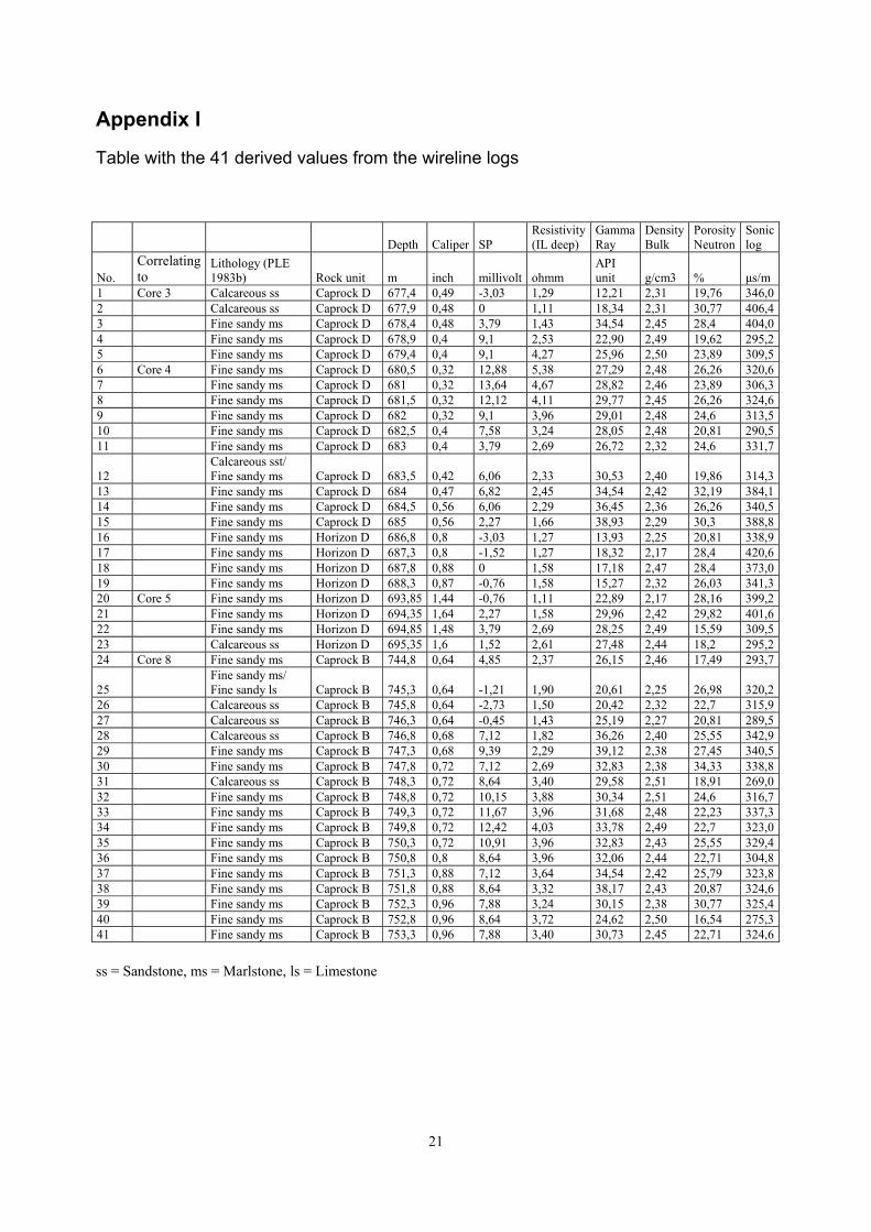
Appendix I Table with the 41 derived values from the wireline logs

Depth Caliper SP Resistivity(IL deep)

Gamma Ray

Density Bulk

Porosity Neutron

Sonic log

No. Correlating to

Lithology (PLE 1983b) Rock unit m inch millivolt ohmm

API unit g/cm3 % µs/m

1 Core 3 Calcareous ss Caprock D 677,4 0,49 -3,03 1,29 12,21 2,31 19,76 346,02 Calcareous ss Caprock D 677,9 0,48 0 1,11 18,34 2,31 30,77 406,43 Fine sandy ms Caprock D 678,4 0,48 3,79 1,43 34,54 2,45 28,4 404,04 Fine sandy ms Caprock D 678,9 0,4 9,1 2,53 22,90 2,49 19,62 295,25 Fine sandy ms Caprock D 679,4 0,4 9,1 4,27 25,96 2,50 23,89 309,56 Core 4 Fine sandy ms Caprock D 680,5 0,32 12,88 5,38 27,29 2,48 26,26 320,67 Fine sandy ms Caprock D 681 0,32 13,64 4,67 28,82 2,46 23,89 306,38 Fine sandy ms Caprock D 681,5 0,32 12,12 4,11 29,77 2,45 26,26 324,69 Fine sandy ms Caprock D 682 0,32 9,1 3,96 29,01 2,48 24,6 313,510 Fine sandy ms Caprock D 682,5 0,4 7,58 3,24 28,05 2,48 20,81 290,511 Fine sandy ms Caprock D 683 0,4 3,79 2,69 26,72 2,32 24,6 331,7

12 Calcareous sst/ Fine sandy ms Caprock D 683,5 0,42 6,06 2,33 30,53 2,40 19,86 314,3

13 Fine sandy ms Caprock D 684 0,47 6,82 2,45 34,54 2,42 32,19 384,114 Fine sandy ms Caprock D 684,5 0,56 6,06 2,29 36,45 2,36 26,26 340,515 Fine sandy ms Caprock D 685 0,56 2,27 1,66 38,93 2,29 30,3 388,816 Fine sandy ms Horizon D 686,8 0,8 -3,03 1,27 13,93 2,25 20,81 338,917 Fine sandy ms Horizon D 687,3 0,8 -1,52 1,27 18,32 2,17 28,4 420,618 Fine sandy ms Horizon D 687,8 0,88 0 1,58 17,18 2,47 28,4 373,019 Fine sandy ms Horizon D 688,3 0,87 -0,76 1,58 15,27 2,32 26,03 341,320 Core 5 Fine sandy ms Horizon D 693,85 1,44 -0,76 1,11 22,89 2,17 28,16 399,221 Fine sandy ms Horizon D 694,35 1,64 2,27 1,58 29,96 2,42 29,82 401,622 Fine sandy ms Horizon D 694,85 1,48 3,79 2,69 28,25 2,49 15,59 309,523 Calcareous ss Horizon D 695,35 1,6 1,52 2,61 27,48 2,44 18,2 295,224 Core 8 Fine sandy ms Caprock B 744,8 0,64 4,85 2,37 26,15 2,46 17,49 293,7

25 Fine sandy ms/ Fine sandy ls Caprock B 745,3 0,64 -1,21 1,90 20,61 2,25 26,98 320,2

26 Calcareous ss Caprock B 745,8 0,64 -2,73 1,50 20,42 2,32 22,7 315,927 Calcareous ss Caprock B 746,3 0,64 -0,45 1,43 25,19 2,27 20,81 289,528 Calcareous ss Caprock B 746,8 0,68 7,12 1,82 36,26 2,40 25,55 342,929 Fine sandy ms Caprock B 747,3 0,68 9,39 2,29 39,12 2,38 27,45 340,530 Fine sandy ms Caprock B 747,8 0,72 7,12 2,69 32,83 2,38 34,33 338,831 Calcareous ss Caprock B 748,3 0,72 8,64 3,40 29,58 2,51 18,91 269,032 Fine sandy ms Caprock B 748,8 0,72 10,15 3,88 30,34 2,51 24,6 316,733 Fine sandy ms Caprock B 749,3 0,72 11,67 3,96 31,68 2,48 22,23 337,334 Fine sandy ms Caprock B 749,8 0,72 12,42 4,03 33,78 2,49 22,7 323,035 Fine sandy ms Caprock B 750,3 0,72 10,91 3,96 32,83 2,43 25,55 329,436 Fine sandy ms Caprock B 750,8 0,8 8,64 3,96 32,06 2,44 22,71 304,837 Fine sandy ms Caprock B 751,3 0,88 7,12 3,64 34,54 2,42 25,79 323,838 Fine sandy ms Caprock B 751,8 0,88 8,64 3,32 38,17 2,43 20,87 324,639 Fine sandy ms Caprock B 752,3 0,96 7,88 3,24 30,15 2,38 30,77 325,440 Fine sandy ms Caprock B 752,8 0,96 8,64 3,72 24,62 2,50 16,54 275,341 Fine sandy ms Caprock B 753,3 0,96 7,88 3,40 30,73 2,45 22,71 324,6 ss = Sandstone, ms = Marlstone, ls = Limestone

Measured core permeability versus permeability from equation k ½=250*Φ3/Sw

0.000

0.000

0.000

0.010

1.000

100.000

10000.000

1 3 5 7 9 11 13 15 17 19 21 23 25 27 29 31 33

Measured corepermeability

Permeabilityfrom equation

Appendix II The permeability measured from core values versus the calculated permeability

values

Tidigare skrifter i serien”Examensarbeten i Geologi vid LundsUniversitet”:

163. Davidson, Anja, 2003: Ignimbritenheternai Barranco de Tiritaña, övre Mogánforma-tionen, Gran Canaria.

164. Näsström, Helena, 2003: Klotdioriten vidSlättemossa, centrala Småland – mineral-kemi och genes.

165. Nilsson, Andreas, 2003: Early Ludlow(Silurian) graptolites from Skåne, southernSweden.

166. Dou, Marion, 2003: Les ferromagnésiensdu granite rapakivique de Nordingrå –centre-est de la Suède – compositionchimique et stade final de cristallisation.

167. Jönsson, Emma, 2003: En pollenanalytiskstudie av råhumusprofiler från Säröhalvöni norra Halland.

168. Alwmark, Carl, 2003: Magmatisk ochmetamorf petrologi av en mafisk intrusioni Mylonitzonen.

169. Pettersson, Ann, 2003: Jämförande litolo-gisk och geokemisk studie av Sevensamfibolitkomplex i Sylarna och Kebne-kaise.

170. Axelsson, Katarina, 2004: Bedömning avpotentiell föroreningsspridning från ettavfallsupplag utanför Löddeköpinge,Skåne.

171. Ekestubbe, Jonas, 2004: 40Ar/39Argeokronologi och implikationer förtolkningen av den Kaledoniska utveck-lingen i Kebnekaise.

172. Lindgren, Paula, 2004. Tre sensveko-fenniska graniter: kontakt- och ålders-relationer samt förekomst av metasedi-mentära enklaver.

173. Janson, Charlotta, 2004. A petrographicaland geochemical study of granitoids fromthe south-eastern part of the Linderöds-åsen Horst, Skåne.

174. Jonsson, Sara, 2004: Structural control offine-grained granite dykes at the ÄspöHard Rock Laboratory, north of Oskars-hamn, Sweden.

175. Ljungberg, Carina, 2004: Belemnitersstabila isotopsammansättning: paleo-miljöns och diagenesens betydelse.

176. Oster, Jessica, 2004: A stratigraphic studyof a coastal section through a LateWeichselian kettle hole basin at Åla-

bodarna, western Skåne, Sweden.177. Einarsson, Elisabeth, 2004: Morphological

and functional differences betweenrhamphorhynchoid and pterodactyloidpterosaurs with emphasis on flight.

178. Anell, Ingrid, 2004: Subsidence in riftzones; Analyzing results from repeatedprecision leveling of the Vogar Profile onthe Reykjanes Peninsula, SouthwestIceland.

179. Wall, Torbjörn, 2004: Magnetic grain-sizeanalyses of Holocene sediments in theNorth Atlantic and Norwegian Sea –palaeoceano-graphic applications.

180. Mellgren, Johanna, S., 2005: A model ofreconstruction for the oral apparatus ofthe Ordovician conodont genus Proto-panderodus Lindström, 1971.

181. Jansson, Cecilia, 2005: Krossbergskvalitetoch petrografi i den kambriska Harde-bergasandstenen i Skåne.

182. Öst, Jan-Olof, 2005: En övergripandebeskrivning av malmbildande processermed detaljstudier av en bandad järnmalmfrån södra Dalarna, Bergslagen.

183. Bragée, Petra, 2005: A palaeoecologicalstudy of Holocene lake sediments abovethe highest shoreline in the province ofVästerbotten, northeast Sweden.

184. Larsson, Peter, 2005: Palynofacies ochmineralogi över krita-paleogengränsen vidStevns Klint och Kjølby Gaard, Danmark.

185. Åberg, Lina, 2005: Metamorphic study ofmetasediment from the KangilinaaqPeninsula, West Greenland.

186. Sidgren, Ann-Sofie, 2005: 40Ar/39Ar-geokronologi i det Rinkiska bältet, västraGrönland.

187. Gustavsson, Lena, 2005: The Late SilurianLau Event and brachiopods from Gotland,Sweden.

188. Nilsson, Eva K., 2005: Extinctions andfaunal turnovers of early vertebratesduring the Late Silurian Lau Event, Gotland,Sweden.

189. Czarniecka, Ursula, 2005: Investigationsof infiltration basins at the Vomb WaterPlant – a study of possible causes ofreduced infiltration capacity.

190. G³owacka, Ma³gorzata, 2005: Soil andgroundwater contamination with gasolineand diesel oil. Assessment of subsurfacehydrocarbon contamination resulting from

Geologiska institutionenGentrum för GeoBiosfärsvetenskap

Sölvegatan 12, 223 62 Lund

a fuel release from an underground storagetank in Vanstad, Skåne, Sweden.

191. Wennerberg, Hans, 2005: A study of earlyHolocene climate changes in Småland,Sweden, with focus on the ‘8.2 kyr event’.

192. Nolvi, Maria & Thorelli, Gunilla, 2006:Extraterrestrisk och terrestrisk kromrikspinell i fanerozoiska kondenseradesediment.

193. Nilsson, Andreas, 2006: Palaeomagneticsecular variations in the varved sedimentsof Lake Goœci¹¿, Poland: testing thestability of the natural remanent magneti-zation and validity of relative palaeo-intensity estimates.

194. Nilsson, Anders, 2006: Limnologicalresponses to late Holocene permafrostdynamics at the Stordalen mire, Abisko,northern Sweden.

195. Nilsson, Susanne, 2006: Sedimentary faciesand fauna of the Late Silurian Bjärsjö-lagård Limestone Member (KlintaFormation), Skåne, Sweden.

196. Sköld, Eva, 2006: Kulturlandskapets föränd-ringar inom röjningsröseområdet YttraBerg, Halland - en pollenanalytisk under-sökning av de senaste 5000 åren.

197. Göransson, Ammy, 2006: Lokala miljö-förändringar i samband med en plötslighavsyteförändring ca 8200 år före nutidvid Kalvöviken i centrala Blekinge.

198. Brunzell, Anna, 2006: Geofysiska mät-ningar och visualisering för bedömningav heterogeniteters utbredning i en isälvs-avlagring med betydelse för grundvatten-flöde.

199. Erlfeldt, Åsa, 2006: Brachiopod faunaldynamics during the Silurian Ireviken Event,Gotland, Sweden.

200. Vollert, Victoria, 2006: Petrografisk ochgeokemisk karaktärisering av metabasiteri Herrestadsområdet, Småland.

201. Rasmussen, Karin, 2006: En provenans-studie av Kågerödformationen i NV Skåne– tungmineral och petrografi.

202. Karlsson, Jonnina, P., 2006: An

investigation of the Felsic Ramiane Pluton,in the Monapo Structure, NorthernMoçambique.

203. Jansson, Ida-Maria, 2006: An Early Jurassicconifer-dominated assemblage of theClarence-Moreton Basin, easternAustralia.

204. Striberger, Johan, 2006: En lito- och bio-stratigrafisk studie av senglaciala sedimentfrån Skuremåla, Blekinge.

205. Bergelin, Ingemar, 2006: 40Ar/39Ar geo-chronology of basalts in Scania, S Sweden:evidence for two pulses at 191-178 Maand 110 Ma, and their relation to the break-up of Pangea.

206. Edvarssson, Johannes, 2006: Dendro-kronologisk undersökning av tallbeståndsetablering, tillväxtdynamik och degene-rering orsakat av klimatrelaterade hydro-logiska variationer på Viss mosse ochÅbuamossen, Skåne, södra Sverige, 7300-3200 cal. BP.

207. Stenfeldt, Fredrik, 2006: Litostratigrafiskastudier av en platåformad sand- och grus-avlagring i Skuremåla, Blekinge.

208. Dahlenborg, Lars, 2007: A Rock MagneticStudy of the Åkerberg Gold Deposit,Northern Sweden.

209. Olsson, Johan, 2007: Två svekofenniskagraniter i Bottniska bassängen; utbredning,U-Pb zirkondatering och test av olikaabrasionstekniker.

210. Erlandsson, Maria, 2007: Den geologiskautvecklingen av västra Hamrångesyn-klinalens suprakrustalbergarter, centralaSverige.

211. Nilsson, Pernilla, 2007: Kvidingedeltat –bildningsprocesser och arkitektoniskuppbyggnadsmodell av ett glacifluvialtGilbertdelta.

212. Ellingsgaard, Óluva, 2007: Evaluation ofwireline well logs from the boreholeKyrkheddinge-4 by comparsion tomeasured coredata.

Evaluation of wireline well logs from the borehole ...

Documents

Transcript of Evaluation of wireline well logs from the borehole ...