Evaluation of TOYOCRYPT-HR1

January 17, 2001

Information Security Research Centre Queensland University of Technology

Ed Dawson, Andrew Clark, Helen Gustafson, Bill Millan, Leonie Simpson

TABLE OF CONTENTS 1 Executive Summary ...............................................................................................3 2 Description of TOYOCRYPT-HR1.......................................................................4

2.1 Notation ..........................................................................................................4 3 Structural Aspects ..................................................................................................4

3.1 LFSR Operation .............................................................................................4 3.2 Analysis of the nonlinear function.................................................................4 3.3 Key Management ...........................................................................................6 3.4 Modes of Operation .......................................................................................6

4 Keystream Properties .............................................................................................6 4.1 Period .............................................................................................................7 4.2 Linear Complexity .........................................................................................7 4.3 Statistical Analysis.........................................................................................7 4.4 Entropy...........................................................................................................8

4.4.1 Entropy of Input Sequence.....................................................................8 4.4.2 Entropy of Output Sequence..................................................................8

5 Possible Attacks .....................................................................................................9 5.1 Simple Attacks ...............................................................................................9 5.2 Divide and Conquer Attacks..........................................................................9

5.2.1 Attack procedure..................................................................................10 5.2.2 Attack algorithm ..................................................................................10 5.2.3 Implementation issues for the attack....................................................11 5.2.4 Attack complexity................................................................................11

5.3 Correlation Attacks ......................................................................................12 5.3.1 Fast Correlation Attacks ......................................................................12 5.3.2 Linear Cryptanalysis ............................................................................12 5.3.3 Conditional Correlation Attacks ..........................................................13 5.3.4 Inversion Attack...................................................................................13

5.4 Discussion ....................................................................................................13 6 Implementation ....................................................................................................14

6.1 Software .......................................................................................................14 6.2 Hardware......................................................................................................14 6.3 Key Generation ............................................................................................15

7 Conclusion ...........................................................................................................16 8 References............................................................................................................16 9 Appendices...........................................................................................................19

2

Evaluation of TOYOCRYPT-HR1 Algorithm 1 Executive Summary This is a report on the analysis of the Pseudorandom Number Generator (PRNG), TOYOCRYPT-HR1. For this algorithm the evaluators have

(i) analysed structural aspects; (ii) evaluated basic cryptographic properties; (iii) measured the entropy; (iv) evaluated security from attack; (v) evaluated statistical properties; (vi) surveyed the speed.

The TOYOCRYPT-HR1 algorithm is a standard design for a PRNG using a linear feedback shift register (LFSR) together with a nonlinear Boolean function. This design produces a sequence with provable security properties in relation to period and high linear complexity. The sequences analysed displayed white-noise statistics and high entropy. The algorithm is secure from standard cryptographic attacks including linear cryptanalysis and correlation attacks. However, the evaluators have identified three different flaws with the algorithm. Flaw 1 Divide and Conquer Attack There is a possible divide and conquer attack which is significantly faster than exhaustive key search. We have described a simple method to change the algorithm to correct this flaw. Flaw 2 Operational Speed in Software The algorithm is very slow in software for many applications. The designers of the algorithm have recognised this problem and have included a parallel mode of operation to increase speed. However, it should be noted that this will also increase the key length and further this adaption can be applied to most PRNG’s. Flaw 3 Key Generation The process of using the key to generate a new primitive polynomial is very slow for many applications. The evaluators are of the opinion that due to this problem a fixed LFSR will need to be used in many applications.

3

2 Description of TOYOCRYPT-HR1 The TOYOCRYPT-HR1 pseudorandom sequence generator consists of a single regularly clocked 128-bit linear feedback shift register (LFSR) and a nonlinear Boolean function, f, of 127 input variables. The function f is used as a nonlinear filter function, and the generator is known as a nonlinear filter generator. The algebraic normal form of function f is given in Appendix B. The keystream is generated by applying the nonlinear function f to the contents of 127 of the 128 stages of the LFSR. Each time the LFSR is clocked, an output bit is produced. The TOYOCRYPT-HR1 keystream generator has two 128-bit keys: a fixed key and a stream key. The fixed key consists of the coefficients of the LFSR characteristic polynomial, and is selected such that the characteristic polynomial is primitive and irreducible on F2. There are approximately 2120 such polynomials. The stream key is used to form the LFSR initial state, and is an arbitrary 128 bits, except for the all zero initial state. Thus there are 2128 – 1 possible stream keys. Hence, the effective key size is 248.

2.1 Notation Let the LFSR output sequence be denoted d . Let the contents of the 128 stages of the LFSR at time t be denoted x

∞== 0)}({ ttd

0(t), x1(t), … , x127(t). Then d(t) = x0(t-1), for t ≥ 1. Denote the sequence of inputs to the filter function f as ∞

== 0)}({ ttXXwhere X(t) = {x0(t), x1(t), …, x125(t), x127(t)}. Note that x126(t) is not used as input to f. Then the output sequence of the nonlinear filter generator is the keystream

, where z(t) = f(X(t)), for t ≥ 0. ∞== 0)}({ ttzz

3 Structural Aspects

3.1 LFSR Operation The LFSR uses a Galois configuration rather than the more standard Fibonacci configuration. The Galois configuration offers a significant increase in speed over the Fibonacci configuration in both software and hardware. In software we would estimate on the average about a four to five times improvement in speed. The speed of an LFSR implemented using the Galois configuration is independent of the number of taps in the feedback polynomial since it does not require individual bits to be extracted for use in calculating the next output bit. The Galois configuration also has the effect that LFSR state bits change in time (due to XOR with the feedback bit).

3.2 Analysis of the nonlinear function Linear feedback shift registers are commonly used in pseudorandom number generators, as the properties of sequences produced by LFSRs are well known, their implementation in hardware or software is easy, and they allow for fast encryption and decryption rates. However, LFSR sequences are easily predicted from a short segment. For an LFSR of length 128, the entire period of the LFSR output sequence can be determined from only 128 successive terms in the sequence if the feedback polynomial is known, and from only 256 successive bits if the feedback polynomial is unknown [MASS 69]. This vulnerability to known plaintext attacks makes LFSRs unsuitable for use as pseudorandom sequence generators on their own. One way to

4

make use of the good properties of LFSR sequences while avoiding the weakness due to their linearity is to introduce nonlinearity by using a nonlinear Boolean function operating on the contents of several stages of a regularly clocked LFSR. The choice of Boolean function used contributes significantly to the cryptographic security of the pseudorandom sequence generator. In this section, the Boolean function f, used as nonlinear combining function in the TOYOCRYPT-HR1 pseudorandom sequence generator, is examined. The nonlinear feedforward function f is a Boolean function that takes as input the contents of 127 of the 128 stages of the LFSR and produces a single output bit. In [SPEC HR1] it is described as , although, as x2

1282: FFf →

21272: FF →

126(t) is not used in f, it is more properly described as . For simplicity, in this section of the report, denote the contents of the stages of the LFSR as x

f0, x1, x2,… x127. (that is, drop the (t)).

As in [SPEC HR1], consider the following division of the LFSR: X = {x127, x126, XL , XR,} where XL = {x125, x124, … , x63} and XR = {x62, x61, … , x0}. The function f consists of a single linear term, sixty-three quadratic terms, and three other terms of orders four, seventeen and sixty-three, respectively. The linear term is x127. The quadratic terms are products, each with one factor from XL and the other from XR. Note that all terms of order greater than two are products for which all factors are stages within XR. This is a potential weakness, which may be exploited in a divide and conquer style attack (see Section 5.2). A basic condition for nonlinear filter generators for cryptographic applications is that the output sequence is balanced. This is true only if the combining function f is balanced. As the function f is linear in the variable x127, then it is balanced. Thus the symbol frequency of the output sequence, z, is the same as for the underlying LFSR sequence, d. The nonlinearity of a Boolean function is defined to be the minimum Hamming distance between the function and any affine function. If the nonlinearity is low, then the function is closely approximated by an affine function, a weakness which is exploited by fast correlation attacks. For Boolean functions with an even number of

inputs, n, the maximum nonlinearity is known to be 1

21 22−− −

nn , and is obtained by a

class of Boolean function known as bent functions. The subfunction h is a bent function (note that ) of 126 variables, with nonlinearity N127xhf += h = 2125- 262 (see [ROTH 76]). Bent functions are not balanced, so are unsuitable for use as combining functions. The function f has a bent subfunction, to provide high nonlinearity, but has an additional linear term to provide balance. For the function f, with n = 127, the nonlinearity is 2126 – 263. This implies that the bias available to any linear correlation is upper bounded by 2-64. This value is sufficiently low to provide security (see Section 5). Further examination of the quadratic terms of the function f was performed. For each quadratic term xixj, i ∈ XR and j ∈ XL, the difference j-i was calculated. The differences range in value from 17 (for x62x79) to 102 (for x17x119 and x19x121). Interestingly, as illustrated by the last example, the differences are not necessarily unique. Differences of 34, 48, 53, 56,66,69,70,89,91,96 and 102 each occur for two terms, the difference 50 occurs for three terms, and the difference 72 occurs for 4 terms (see Appendix C). The existence of multiple quadratic terms with common differences is a potential weakness. As an example to illustrate the way this can be

5

exploited, consider the two quadratic terms x3x75 and x6x78. Whatever the value of the term x3x75, after clocking the LFSR three times, this value is now held by x6x78 (with due allowance for the Galois configuration of the LFSR). There are sixty-three quadratic terms, so the proportion of quadratic terms with common differences is quite small, and perhaps cannot be fully exploited in an attack. However, changing the arrangement of the quadratic terms in the filter function could eliminate this potential weakness entirely. A simple way to do this is to select a different 63 bit permutation.

3.3 Key Management There is a 256 bit key which has two components. One component is 128 bits, called the stream key, which is used as initial state vector for LFSR. A second component is 128 bits, called the fixed key, which is used to generate primitive polynomials to define tap settings for LFSR using Algorithm 4.6 from [SPEC HS1]. This process is very slow (see Section 6.3) since many different fixed keys would need to be tested before a primitive polynomial is found. The time taken for this process may cause problems in certain applications as explained further below. In certain applications it is possible to overcome this problem with having to check multiple fixed keys by having the primitive polynomial generated offline. This process works well in key management processes called key transport where one party in the communication process actually creates keys. However there are many key management protocols where this is not possible. For example, in the key agreement process which uses the Diffie-Hellman Key Agreement algorithm each party in a key generation process inputs a random number. These are combined together to form the actual key using exponentiation process. This process in most applications needs to be done online. This is very costly in terms of time and communication bandwidth if this process is required to be repeated multiple times. It is the opinion of the evaluators, due to the above problem with the generation of primitive polynomials, that in many applications a fixed LFSR will be used. This reduces the key to the 128 bit initial state vector of LFSR.

3.4 Modes of Operation The TOYOCRYPT-HR1 algorithm is especially slow in software. In order to overcome this problem the designers have included a parallel mode of operation. This involves the generation of n independent sequences in parallel (see [SPEC HR1]) where n is less than or equal to the word size of the processor. This leads to higher speed for keystream generation (see Section 6.1). There is nothing unique about this process. This method can be applied to almost any keystream generator. However, it should be noted that a much larger key size is required for this parallel mode. 4 Keystream Properties For keystream sequences to be used in stream ciphers which provide cryptographic security, the keystream must possess certain basic properties. These include a large period, large linear complexity and white-noise statistics. Experimental results, which are included below for linear complexity and statistical analysis, were obtained by the evaluators using the CRYPT-X package. This is a statistical package which was designed previously by the evaluators for analysing

6

encryption algorithms. The relevant pages from the CRYPT-X manual have been included as Appendix A.

4.1 Period The keystream properties cited in [EVAL HR1] relating to period were verified. That is, for the TOYOCRYPT-HR1 keystream generator, the period of the sequence produced by the keystream generator is Pz = 2128 –1.

4.2 Linear Complexity The linear complexity test checks for the minimum amount of knowledge required to reconstruct the whole stream using a linear feedback shift register. It is difficult to determine exactly the linear complexity of a sequence from TOYOCRYPT-HR1 equal in length to the complete period. However, bounds for this linear complexity can be found. The evaluators are in agreement with the results in [EVAL HR1] that the linear complexity of a keystream sequence of length Pz has a lower and upper bound of 2124 and 2127. The selection of higher products of degree 2, 4, 17 and 63 means that the linear complexity profile of the keystream should approximately follow the n/2 line for strings of length n. In order to obtain empirical evidence for the linear complexity and linear complexity profile we applied the tests from the CRYPT-X package. These linear complexity tests were applied to ten TOYOCRYPT-HR1 output bit-streams each of length 106 bits. The results gave linear complexity values extremely close to that expected for random data (i.e. half the bit-stream length). For more detailed results see Appendix D. The results for the linear complexity profile indicate that, as the bit-stream increases in length, the changes in linear complexity maintain the expected value of half the stream length. These results demonstrate that the whole bit-stream is required to re-construct the stream itself - thus giving an attacker no advantage in being able to create the bit-stream with a smaller number of output bits.

4.3 Statistical Analysis A preliminary statistical analysis was carried out on TOYOCRYPT-HR1, in order to confirm the results in [EVAL HR1]. This analysis included three tests, namely a bit-frequency test, a subblock test on 4-bit subblocks, and a runs distribution (including the longest run). The tests were applied to 100 streams of length 20,000 bits each. The test results show that 9 of the 300 tests (or 0.03) gave p-values below 0.05. These results support the randomness of the TOYOCRYPT-HR1 output. The evaluators confirmed these results using the CRYPT-X package. Further statistical analysis was carried out by the evaluators. The above tests plus additional statistical randomness tests from CRYPT-X were applied to much longer output streams from TOYOCRYPT-HR1. A further measure of sequence complexity was added to check the period of the output stream. The tests are based on the hypothesis that the measure obtained from the output stream supports randomness. The p-values obtained for the tests represent the probability that such a sample result would be obtained if the algorithm produces a random stream. Very small p-values would support non-randomness. The sequence complexity test was applied to binary output streams of 106 bits (due to the amount of time required for the test), using ten different keys. The remaining tests were applied to ten binary output streams of 107 bits.

7

The subblock tests were applied to the output stream by dividing the bit-stream into non-overlapping subblocks of lengths ranging from 2 to 30 bits. The maximum subblock length of 30 was determined from the length of the file and the limitations of the test applied. Statistical Analysis Results The results of the CRYPT-X tests are summarised using p-values in Appendix E. The lowest p-value for any one test is 0.0007, with 24 of the 340 p-values obtained falling below 0.05. This represents a proportion of 0.07 of the tests applied, which is above the 0.05 level, yet not significant. Hence these results supports the randomness of the output from TOYOCRYPT-HR1.

4.4 Entropy We can measure the entropy of TOYOCRYPT-HR1 in relation to the entropy of the input sequence and the output sequence.

4.4.1 Entropy of Input Sequence The entropy of input sequence relates to the uncertainty of finding the state vector of the LFSR. For discussions on how difficult this is, we refer to Section 5 of this report on possible attacks, since the aim of most of these attacks is to find this state vector in less than exhaustive search.

4.4.2 Entropy of Output Sequence In order to measure the entropy of the output sequence of TOYOCRYPT-HR1 we divided the output of sequence into subblocks. The analysis of subblock patterns is an important measure of the entropy of sequences produced by PRNG’s. The test applied gives the entropy of a b-bit subblock as the number of independent bits per subblock generated. Additional tests include the distribution of ones in these b-bit subblocks and the distribution of ones in the binary derivative of these blocks. For further explanation of these tests see the CRYPT-X manual (Appendix A). These tests were applied to one large sample of 1 Gigabyte of output from TOYOCRYPT-HR1. The entropy test was applied to subblocks of length 48. No larger subblock lengths could be taken, as a much larger file would be required, that exceeded the storage limitation of the computer. The CRYPT-X package requires a considerably longer output stream than 1 Gigabyte to investigate the entropy of subblocks larger than 48 bits, as it will only break larger subblocks into 48-bit blocks and give no further information than what has been obtained on the 48-bit subblock entropy value. To investigate larger subblocks alternative tests were applied with the subblock length ranging from 56 to 1024. These tests were based on the hypothesis that the ones are distributed independently and symmetrically, and the hypothesis that the runs are distributed independently and symmetrically, in the subblock. Entropy Tests Results For a bit-stream of 1 Gigabyte the longest subblock that could be tested using the 'repetition test' applied was 48 bits. Results give a strong emphasis that full entropy exists. This means that there are 48 independent bits per 48-bit block, and so any set of 48-bit subblocks obtained from a TOYOCRYPT-HR1 output stream will appear to be randomly generated.

8

For subblocks lengths from 56 to 1024 the distribution of ones and the distribution of runs (binary derivative) in the b-bit subblock are distributed independently and symmetrically (see Appendix F). This gives support to maximum entropy of the output from TOYOCRYPT-HR1 for subblocks of length from 56 to 1024. 5 Possible Attacks In this section of the report, possible known plaintext attacks on the nonlinear filter generator are investigated. It is assumed in the discussion that the structure of the generator is known to an attacker, and that only the keys are unknown. For most of these attacks, the discussion assumes that the fixed key (the LFSR feedback function) is known, and only the stream key (that is, the initial state of the LFSR) is unknown. Such a situation is possible, as it is likely that the fixed key can be obtained through reverse engineering (if in hardware), or by examining source code (if in software). Note that if the attacks on the nonlinear filter generator are unsuccessful when the fixed key is known, then they will also be unsuccessful when the fixed key is unknown. Generally, in the case where both the stream key and the fixed key are unknown, the computational complexity of attacks on the generator is equal to the computational complexity of the attack for a known fixed key multiplied by 2120 (the number of possible LFSR feedback functions). However, this is not always the case. For example, the simple attack based on linear complexity [MASS 69] does not require knowledge of the LFSR feedback function, or even the length of the LFSR, so the complexity of this attack is unchanged by knowledge of the fixed key. However, all of the more sophisticated attacks outlined in Section 5.2 and 5.3 below require knowledge of this LFSR. Hence, in the case where the LFSR is unknown the complexity of each attack should be multiplied by a factor of 2120.

5.1 Simple Attacks There are four simple, classical attacks on pseudorandom sequence generators. These are brute force attacks, in which exhaustive search of the keyspace is conducted; attacks based on short period; attacks based on low linear complexity and statistical attacks where the output sequence is sufficiently non-random. Assuming the fixed key is known, for a brute force attack on the TOYOCRYPT-HR1 pseudorandom sequence generator, there are 2128–1 stream keys to be tested. For an attack based on repetition of the period, more than 2128–1 bits of keystream must be observed. Similarly, an attack based on the linear complexity would require a known keystream segment of at least 2125 bits, and very likely more, say 2128 bits. The statistical analysis described in Section 4.3 identified no weakness which could be used in an attack. Thus the TOYOCRYPT-HR1 keystream generator is resistant to these simple attacks, as the keyspace is too large to permit exhaustive search, the period and linear complexity are too high to be the basis of attacks and subsequences examined displayed white-noise statistics.

5.2 Divide and Conquer Attacks Divide and conquer attacks are commonly applied to keystream generators with multiple component LFSRs. The attacks work on the components of the generator separately and sequentially solve for the individual subkeys, generally the initial states of the component LFSRs. This style of attack is not commonly used on nonlinear

9

filter generators, as these have a single LFSR. However, as noted in Section 3, the inputs to the function come from distinct sections of the LFSR: XL, XR, and x127. This property of the Boolean function f may be exploited in an attack performed in a divide and conquer manner by considering these sections of the LFSR as separate components. A similar approach was used to attack the ORYX cipher [WAGN 98]. The attack is conducted under the assumption that the fixed key (the LFSR feedback function) is known. An outline of the procedure for a divide and conquer attack on the TOYOCRYPT-HR1 keystream generator follows.

5.2.1 Attack procedure The attack targets XR. For an assumed initial state of XR, the values of the terms of f of order greater than two are known, and one factor in each of the quadratic terms is also known. Thus the keystream bit can be equated to a known linear combination of x127 and some of the bits of XL. The identity of these bits is known from a combination of the known quadratic terms in the filter function together with the assumed value of XR. A branching search process using a linear consistency test [ZENG 90] can be used to determine whether the guessed initial state of XR was correct. The search process in the attack procedure is iterative. In each iteration, a value for x127 is guessed, a linear equation obtained, and a consistency check made. If the equation is consistent with previous linear equations, the guessed value of x127 and the known feedback function are used to step the LFSR. The process is repeated, forming a path of successive consistent guesses. Note that each guess involves choosing one of two possible values for x127, and so marks a branching point on the path. Note also that each time the LFSR is stepped, another bit of XL is obtained, reducing the number of unknown variables in the subsequent linear equations. If, in some iteration, a linear equation is obtained which is inconsistent with previous equations, then assume that a guessed value of x127 is incorrect. Retrace the path of guesses to the last branching point. Discard all linear equations obtained after this point. Change the guessed value, and begin to trace out another path. If all possible paths result in inconsistencies, then the guessed initial state of XR was incorrect.

5.2.2 Attack algorithm Input:The LFSR feedback polynomial; the observed segment of the pseudorandom output sequence of length N, { . 1

0)}( −=

Nttz

1. Set t=0. Initially, the pool of linear equations is empty. 2. Guess the contents of XR(t). 3. Guess the contents of x127(t). Note this is a branching point. 4. Substitute values from XR(t) and x127(t) into f to form a linear equation in terms of bits

of XL Equate to the known keystream bit z(t). 5. Check whether the new linear equation is consistent with all previous equations in

pool. If consistent, add to pool. If inconsistent, go to Step 7. 6. Increment t. If t≤N, step the LFSR, using the known feedback function and the

guessed value of x127(t) and go to Step 3. If t>N, go to Step 10. 7. Go back along the path of guesses for x127(t) to the last branching point. Change

the value of t to reflect this retracing of the path. Delete from the pool those linear equations obtained after this point. Change the value of x127(t), and note that this is no longer a branching point. Go to Step 4.

10

8. If all paths are searched without finding a path of consistent guesses equal to the length of the known keystream, then the guessed contents of XR(0) were obviously wrong. Go to Step 1.

9. Correct guess for XR forms part of LFSR initial state, use correct path of guessed values of x127 to recover the rest of the LFSR initial state.

10. Stop the procedure. Output: Initial state of LFSR.

5.2.3 Implementation issues for the attack The attack involves guessing the initial contents of XR, assuming the guess to be correct, using this guess and the further guessed contents of x127 to form a pool of linear equations, and testing whether each new linear equation is consistent with those already in the pool. If inconsistencies arise for a guessed value of x127, we conclude that the guessed value was incorrect.

5.2.3.1 False alarms A false alarm occurs when a wrong guess is not detected; that is, when the linear equations are consistent, even though the initial guess for XR is incorrect. Note that the guessed value of XR and the first guessed value of x127 are used to form the first linear equation in the pool. As this is the first equation, no inconsistencies will be detected at this point. However, as the iterative process continues, each guessed value of x127 gives an extra linear equation, while removing one variable. That is, for the first iteration, we have one linear equation in (potentially) 63 variables, for the second iteration, we have two linear equations in 62 variables, and so on. If our path of guessed values continues, by the 32nd iteration, there will be 32 linear equations in 32 variables. Of course, it is possible that inconsistencies will have been detected before reaching this point. Certainly it is unlikely that an incorrect initial state will produce a set of consistent linear equations for many iterations past this. The probability of detecting a wrong guess increases with each iteration.

5.2.3.2 Missing the event Missing the event occurs when the correct initial state is not identified. In this case, if the initial value of XR, and subsequent path of values for x127 are guessed correctly, then all linear equations will be consistent. Thus, the correct initial state will always be identified when tested. The probability of missing the event is zero.

5.2.3.3 Effect of length of known keystream This is a known plaintext attack. To perform this attack, at least 65 bits of the pseudorandom output sequence must be known. One bit of keystream is required for each guessed value of x127 and, after the initial guess of XR, a path of 65 consecutive correct guesses for x127 is required to fill the LFSR. Additional bits can be used to resolve any possible ambiguity.

5.2.4 Attack complexity This divide and conquer attack requires exhaustive search of the keyspace for XR, and a linear consistency test for each additional guess of x127. For the correct initial state of XR, a series of 128 – 63 = 65 correct guesses of x127 is needed to complete the recovery of LFSR initial state. For a wrong guess of XR, inconsistencies in the pool of linear equations should be detected before more than 32 iterations of the algorithm. The complexity of the divide and conquer attack is therefore expected to be O(295). It should be noted that this is only an approximation of the complexity. Due to the magnitude of this complexity no computer simulations to verify this value have been

11

performed. As noted above, there are many uncertainties in the attack model making it difficult to determine the probability of a false alarm.

5.3 Correlation Attacks Divide and conquer correlation attacks had their origin in a paper by Siegenthaler in 1985 [SIEG 85], in which an attack on a nonlinear combiner generator was presented. The attack is based on a model in which the keystream is viewed as a noisy version of an underlying LFSR sequence, with the noise assumed to be additive and independent of the underlying sequence. The correlation between each of the inputs to a combining function and the output could be exploited, to sequentially recover the initial states of the component LFSRs. The attack required sequential exhaustive search of the initial states of the component LFSRs, so would perform no better than exhaustive search if applied to a nonlinear filter generator.

5.3.1 Fast Correlation Attacks Fast correlation attacks are correlation attacks that outperform exhaustive search over the initial states of the component LFSRs. Meier and Staffelbach proposed such an attack on the nonlinear combiner generator in 1989 [MeSt 89]. The attack was modified and applied to the nonlinear filter generator by Forre [FORR 90]. However, the complexity of this attack is still exponential in the length of the LFSR. If applied to TOYOCRYPT-HR1, the complexity would be O(2128), which is infeasible. Additionally, the success of the attack is dependent on the values of crosscorrelation between the output sequence and the underlying LFSR; for crosscorrelation values which are much less than 75%, as is the case for TOYOCRYPT-HR1, the attack is not successful.

5.3.2 Linear Cryptanalysis Linear cryptanalysis of stream ciphers was investigated using a linear sequential circuit approximation by Golic [GOLI 94]. This attack was applied to nonlinear filter generators in [SALM 97]. This attack is a more efficient fast correlation attack on the nonlinear filter generator than that described in Section 5.3.1. The attack is based on a model in which the keystream is regarded as a noisy version of some linear transform of the underlying LFSR sequence, with the probability of noise different from one half [GOLI 96]. Hence the keystream sequence satisfies the same linear recurrence as the LFSR sequence, again with probability different from one half. It was shown that fast correlation attacks using iterative probabilistic error correction can be successfully applied to the nonlinear filter generator provided the level of noise is not too close to 0.5, and if enough low weight parity checks can be obtained. The probability of noise depends on the correlation coefficients of the filter function to linear functions, and may be close to 0.5 if the filter function is close to a bent function. The precomputational complexity of this attack is exponential in the number of inputs to the filter function, and the computational complexity is proportional to the length of known keystream and the average number of parity-checks per bit used. For the filter function specified for TOYOCRYPT-HR1, the number of inputs to the filter function makes the attack infeasible, as the precomputational complexity is O(2127). Additionally, the probability of noise (as calculated in [EVAL HR1]) is given by 642

21 −−=p . This noise value is so close to

0.5 that unconditional fast correlation attacks will not be successful, regardless of the existence or otherwise of the low-weight parity check polynomials these attacks require.

12

5.3.3 Conditional Correlation Attacks The attacks outlined above are unconditional correlation attacks. There exist other conditional correlations in nonlinear filter generators that have been exploited in attacks. In [ANDE 95] an augmented filter function is considered, so that the correlation between blocks of successive input and output bits may be considered. The attack requires precomputation with computational complexity exponential in four times the number of LFSR stages spanned by the inputs to the filter function, that is O(2512), and so is infeasible to apply to TOYOCRYPT–HR1.

5.3.4 Inversion Attack Another attack on nonlinear filter generators is the inversion attack [GOLI 96]. For this attack, the nonlinear filter generator is viewed as a finite input memory combiner, with one input and one output. The input memory space is the number of LFSR stages spanned by the inputs to the filter function. Although not a correlation attack, the inversion attack essentially exploits the correlation to recover the unknown LFSR sequence from an assumed input memory state. The computational complexity of the attack is exponential in the size of the input memory space. For TOYOCRYPT-HR1, the input memory space is 128, and so the computational complexity is O(2128). Therefore it is infeasible to apply the inversion attack to TOYOCRYPT–HR1.

5.4 Discussion In this section of the report, the security of the TOYOCRYPT-HR1 pseudorandom sequence generator has been examined with respect to common attacks on LFSR-based keystream generators. The TOYOCRYPT-HR1 design produces sequences with long period and large linear complexity, so that simple attacks based on these properties are infeasible. Also, the large number of inputs and high nonlinearity of the filter function f provides resistance to correlation attacks, including fast correlation and conditional correlation attacks, and to the inversion attack. These attacks were examined under the assumption that the structure of the generator was known to the cryptanalyst, and that only the stream key was unknown. The attacks were no better than a brute force attack: an exhaustive search of the stream key keyspace. Of the possible attacks examined, only a divide and conquer attack outperformed the brute force attack. In the case where the LFSR is known the expected complexity of the divide and conquer attack is O(295), a considerable reduction from the 2128 possible stream keys. In the case where the LFSR is not known this complexity should be multiplied by 2120. Note that it may be possible to slightly reduce the complexity of this attack by using the repeated common differences in quadratic terms described in Section 3.3. The amount of known plaintext required for this attack is extremely small, only 65 bits. The divide and conquer attack is possible only because of a feature of the filter function f: all of the inputs to the higher order terms of the function come from XR, a 63-bit section of the LFSR. This attack can be made more difficult by a minor adjustment to f. By taking the inputs to these higher order terms from stages spanning the entire LFSR, the attack becomes infeasible. This minor adjustment will retain the nonlinearity and balance of f provided that the constraints of the bent function construction are satisfied, (see [ROTH 76]).

13

6 Implementation As discussed above, the structure of TOYOCRYPT-HR1 is relatively standard for a stream cipher. It uses standard components, namely a linear feedback shift register (LFSR) and a nonlinear Boolean function. The Galois representation of the LFSR is used to enhance the efficiency of its implementation. This is important since the LFSR will generally be the bottleneck in a stream cipher implementation (as it is in this case).

6.1 Software The TOYOCRYPT-HR1 specification [SPEC HR1] describes two software implementations – a serial implementation and a parallel implementation. The parallel implementation is significantly more efficient but implements a slightly different mode of operation in that it generates a number of independent sequences in parallel rather than a single keystream sequence. The evaluators agree with the analysis (in [SPEC HR1], Section 6.3) of the number of operations required in the computation of f (420 operations) and the number of operations required to update the LFSR (639 operations). The total number of operations given for the serial (650) and parallel (1060) implementations for the generation of one and Len bits (where Len is the word size of processor), respectively, also appear to be correct. The serial mode of TOYOCRYPT-HR1 was implemented (but not optimised) in C on an Intel Pentium processor by the review team and was found to run at speeds similar to those reported in the Section 6.2 of [EVAL HR1]. The results of the serial implementation in software show that the cipher will encrypt at only 9.56kbps on a RISC processor at 20MHz. The evaluators agree with the developers comment that an implementation in assembly language would at most improve this speed by a factor of 2 to 3. The speed of the serial implementation in software appears to be far below what is considered acceptable by today’s standards. The parallel implementation generates up to Len independent keystream sequences in parallel. Each of the independent keystreams requires a separate initial state S and feedback polynomial C. The parallel implementation would run approximately 1.6 times slower than the serial implementation but could compute up to Len keystream sequences in parallel. On a 32-bit RISC processor running at 20MHz the parallel implementation will encrypt 32 independent keystreams at an overall rate of 174kbps. This speed would be unacceptable for high bandwidth applications. The bitslice technique presented in the parallel implementation is not specific to the TOYOCRYPT-HR1 algorithm and could be applied to any similar stream cipher which is based on bit operations. The size of the program code for the TOYOCRYPT-HR1 algorithm is extremely small, making it suitable for implementation in devices with memory restrictions such as smart cards.

6.2 Hardware The TOYOCRYPT-HR1 self evaluation report [EVAL HR1] describes the results of simulations of hardware implementations on two different platforms. The first, an

14

FPGA implementation, gives encryption rates of between 81 Mbps (worst case, not optimised for speed) and 418 Mbps (best case, optimised for speed) depending upon the circuit size and for a range of voltages. The second platform tested was a gate array processor with the reported data rates ranging from 223 Mbps (worst case) to 790 Mbps (best case). It was not feasible for the evaluators to verify these results. As expected, hardware implementations of stream ciphers are much faster than software implementations. The encryption rates given for hardware implementations of the TOYOCRYPT-HR1 algorithm are adequate for most applications. For applications requiring very high bandwidths (> 1Gbps) this algorithm would not be suitable.

6.3 Key Generation The TOYOCRYPT-HR1 key includes a 128-bit value, C, which represents the coefficients of a monic primitive polynomial of degree 128. The key setup times quoted in the TOYOCRYPT-HR1 documentation (Section 6.2 of [EVAL HR1]) do not include the non-negligible time required to compute this polynomial. Algorithm 4.6 of [SPEC HR1] describes an algorithm for generating C. This algorithm is identical to previously known techniques [MOV 97] and requires first finding a monic irreducible polynomial before testing that it is primitive. As the self evaluation suggests (Section 3 of [EVAL HR1]), there are precisely:

9976.1192)12( ≈−m

mφ

monic primitive polynomials of degree m=128. This agrees with the TOYOCRYPT-HR1 designers’ evaluation that the effective key space is reduced from 256 bits to 248 bits (128 bits from S and 120 bits from C). The proportion of random monic polynomials of degree m that are irreducible is 1/m. And the complexity of the test for irreducibility is O((lg m)(lg 2)m2) [MOV 97]. For m=128, the proportion of irreducible polynomials that are primitive is approximately:

4992.02

)12( ≈−m

mφ

Thus, on average, one would expect to perform 64 irreducibility tests and two tests of primitiveness to find a suitable C. The high complexity of the tests for irreducibility and primitiveness suggest that the time required to find a suitable polynomial may be considerable. The evaluators performed a software implementation (not optimised for speed) of the algorithm for generating random monic primitive polynomials of degree 128 which took a number of minutes, on the average, to complete. It is expected that a highly optimised implementation would take several seconds to generate a suitable polynomial. This is an important consideration when re-keying of the algorithm is required (see Section 3.3 of this report).

15

7 Conclusion The TOYOCRYPT-HR1 pseudorandom number generator has been designed using a LFSR together with a nonlinear Boolean function. The evaluators agree with the report [EVAL HS1] that the standard keystream properties of large period, large linear complexity and white-noise statistics are satisfied by this generator. However, the evaluators have identified three major areas of concern. Firstly, we have outlined a divide and conquer attack which requires only a small amount of known keystream and has complexity approximately O(2215) if the LFSR is unknown and O(295) if known. In comparison an exhaustive key search has complexity of O(2248) and O(2128) respectively for these two cases. It is possible to prevent this attack by a minor adjustment to nonlinear filter function (see Section 5.4). The second area of major concern relates to the speed of TOYOCRYPT-HR1 in software. The performance of TOYOCRYPT-HR1 in software is very slow. The designers of algorithm have recognised this problem and have included a parallel mode of operation. The evaluators agree that this process will speed up operation. However it should be noted that this will also require a much larger key size. The third major area of concern relates to generation of primitive polynomials as part of the key rather than using a fixed LFSR. As we have noted this process is extremely slow and may not be suitable for many cryptographic applications such as protocols involving Diffie-Hellman key agreement. Due to this it may be necessary to use a fixed LFSR in many applications, reducing the effective key size to 128 bits. The second and third area of concern relate to implementation issues. There seems to be no simple way to overcome these problems. 8 References [ANDE 95] R. J. Anderson, Searching for the optimum correlation attack, In Fast Software Encryption – Leuven’94, Volume 1008 of Lecture Notes in Computer Science, pages 137-143. Springer-Verlag, 1995. [BS 90] E. Biham and A. Shamir, Differential cryptanalysis of DES-like cryptosystems, In Advances in Cryptology – CRYPT0 ’90, Volume 537 of Lecture Notes in Computer Science, pages 2-21. Springer-Verlag, 1991. [EVAL HR1] Self Evaluation Report TOYOCRYPT-HR1. Technical Document, October 2000. [EVAL HS1] Self Evaluation Report TOYOCRYPT-HS1. Technical Document, October 2000.

16

[FORR 90] R. Forre, A fast correlation Attack on nonlinearly feedforward filtered shift-register sequences. In Advances in Cryptology – EUROCRYPT ’89, Volume 434 of Lecture Notes in Computer Science, pages 586-595. Springer-Verlag, 1990. [GOLI 94] J. Golic, Linear cryptanalysis of stream ciphers, In Fast Software Encryption – Leuven’94, Volume 1008 of Lecture Notes in Computer Science, pages 154-169. Springer-Verlag, 1995. [GOLI 96] J. Dj. Golic, On the security of nonlinear filter generators, In Fast Software Encryption – Cambridge’96, Volume 1039 of Lecture Notes in Computer Science, pages 173-188. Springer-Verlag, 1996. [MASS 69] J. L. Massey, Shift Register Synthesis and B.C.H. decoding, IEEE Trans. Inform. Theory, IT-15:122-127, January 1969. [MeSt 89] W. Meier and O. Staffelbach, Fast correlation attacks on certain stream ciphers, Journal of Cryptology, 1(3):159-167, 1989. [MOV 97] A. J. Menezes, P. C. van Oorschot and S. A. Vanstone, Handbook of Applied Cryptography, CRC Press, 1997. [ROTH 76] O. S. Rothaus, On bent functions, Journal of Combinatorial Theory(A), Volume 20, pages 300-305, 1976 [SALM 97] M. Salmasizadeh, L. Simpson, J. Dj. Golic and E. Dawson, Fast correlation attacks and multiple linear approximations, In Information Security and Privacy – ACISP’97, Volume 1270 of Lecture Notes in Computer Science, pages 228-239. Springer-Verlag, 1997. [SIEG 85] T. Siegenthaler, Decrypting a class of stream ciphers using ciphertext only, IEEE Trans. Comput., C-34:81-85, January 1985. [SPEC HR1] Cryptographic Techniques Specifications TOYOCRYPT-HR1. Technical Document, October 2000. [SPEC HS1] Cryptographic Techniques Specifications TOYOCRYPT-HS1. Technical Document, October 2000.

17

[WAGN 98] D. Wagner, L. Simpson, E. Dawson, J. Kelsey, W. Millan and B. Schneier, Cryptanalysis of ORYX, In Workshop on Selected Areas in Cryptography (SAC’98), Volume 1556 of Lecture Notes in Computer Science, pages 296-305. Springer-Verlag, 1998. [ZENG 90] K. C. Zeng, C. H. Yang and T. R. N. Rao, On the linear consistency test (LCT) in cryptanalysis with applications, In Advances in Cryptology – CRYPT0 ’89, Volume 434 of Lecture Notes in Computer Science, pages 164-174. Springer-Verlag, 1990.

18

9 Appendices

19

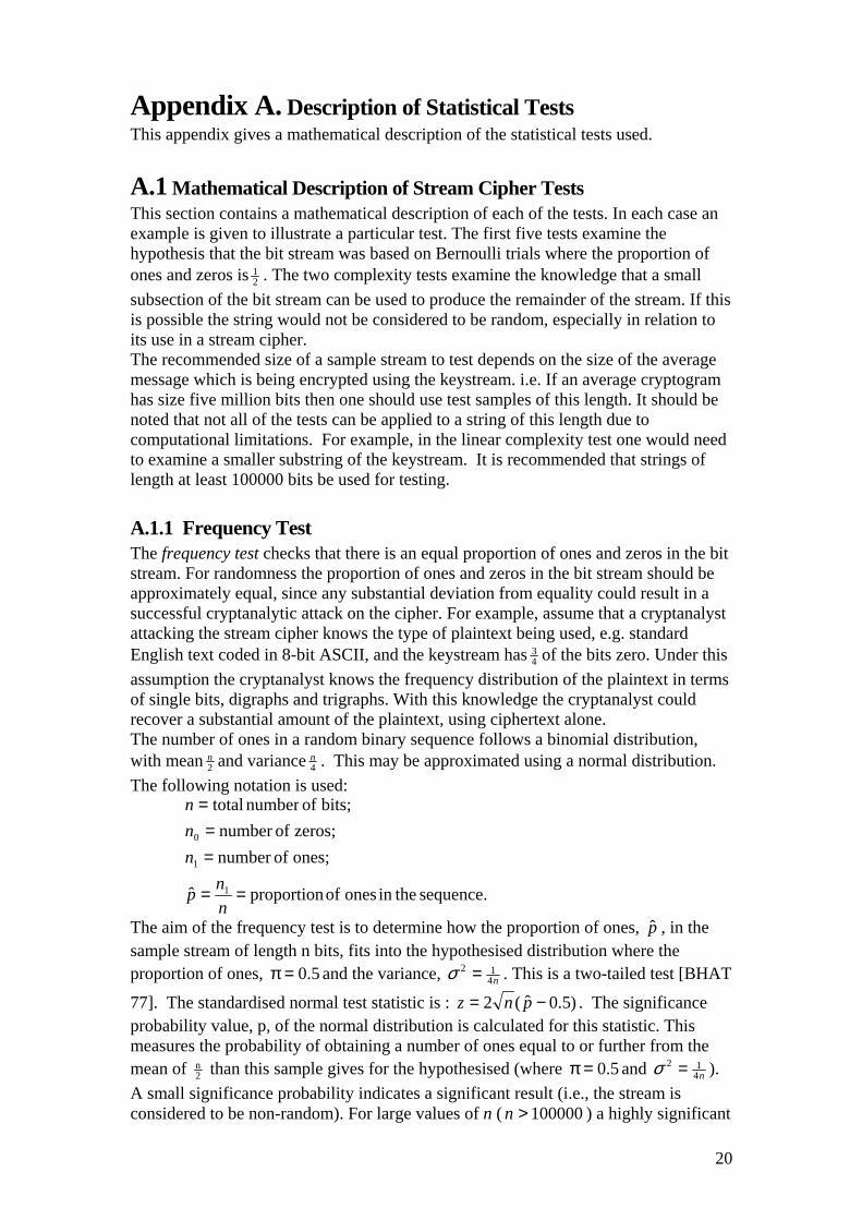
Appendix A. Description of Statistical Tests This appendix gives a mathematical description of the statistical tests used.

A.1 Mathematical Description of Stream Cipher Tests This section contains a mathematical description of each of the tests. In each case an example is given to illustrate a particular test. The first five tests examine the hypothesis that the bit stream was based on Bernoulli trials where the proportion of ones and zeros is 2

1 . The two complexity tests examine the knowledge that a small subsection of the bit stream can be used to produce the remainder of the stream. If this is possible the string would not be considered to be random, especially in relation to its use in a stream cipher. The recommended size of a sample stream to test depends on the size of the average message which is being encrypted using the keystream. i.e. If an average cryptogram has size five million bits then one should use test samples of this length. It should be noted that not all of the tests can be applied to a string of this length due to computational limitations. For example, in the linear complexity test one would need to examine a smaller substring of the keystream. It is recommended that strings of length at least 100000 bits be used for testing.

A.1.1 Frequency Test The frequency test checks that there is an equal proportion of ones and zeros in the bit stream. For randomness the proportion of ones and zeros in the bit stream should be approximately equal, since any substantial deviation from equality could result in a successful cryptanalytic attack on the cipher. For example, assume that a cryptanalyst attacking the stream cipher knows the type of plaintext being used, e.g. standard English text coded in 8-bit ASCII, and the keystream has 4

3 of the bits zero. Under this assumption the cryptanalyst knows the frequency distribution of the plaintext in terms of single bits, digraphs and trigraphs. With this knowledge the cryptanalyst could recover a substantial amount of the plaintext, using ciphertext alone. The number of ones in a random binary sequence follows a binomial distribution, with mean 2

n and variance 4n . This may be approximated using a normal distribution.

The following notation is used:

sequence. theinonesofproportionˆ

ones;ofnumberzeros;ofnumber

bits;ofnumbertotal

1

1

0

==

==

=

nnp

nnn

The aim of the frequency test is to determine how the proportion of ones, , in the sample stream of length n bits, fits into the hypothesised distribution where the proportion of ones, and the variance,

p̂

5.0=π n412 =σ . This is a two-tailed test [BHAT

77]. The standardised normal test statistic is : )5.0ˆ(2 −= pnz . The significance probability value, p, of the normal distribution is calculated for this statistic. This measures the probability of obtaining a number of ones equal to or further from the mean of 2

n than this sample gives for the hypothesised (where and 5.0=π n412 =σ ).

A small significance probability indicates a significant result (i.e., the stream is considered to be non-random). For large values of n ( ) a highly significant 100000>n

20

result (significance probability < 0.001) indicates a possible weakness in the cipher and it is recommended that no further tests be carried out on this sample as the imbalance of ones and zeros may effect their results. It should be noted that passing the frequency test does not mean the stream is not patterned. The following highly patterned streams, where the number of ones and zeros are equal, will pass the frequency test: 11111111..........00000000......... 10101010101010..................... Hence further testing is required to obtain knowledge of any patterns in the stream. Example: Test stream: 10100010000101110001011000111010101010101010000001 Calculations and results:

504

12

50n

×=σ

=

42.0ˆ

211

==

pn

13137.1)5.042.0(50z −=−= 2579.0p =Interpretation:

25.79 % of bit streams of length 50 will have a number of ones equal to or further from the mean of 25, for the hypothesised distribution, than this sample. This sample satisfies the frequency test.

A.1.2 Binary Derivative Test The binary derivative is a new stream formed by the exclusive-or operation on successive bits in the stream. Successive binary derivative streams may be obtained from each new binary derivative, each one being of length one less than its predecessor [CARR 88]. The proportion of ones in the i-th binary derivative gives the proportion of overlapping (i+1)-tuples from the original stream in one of two known groupings of these (i+1)-tuples. This will be explained for i and i . 1= 2=When i (first binary derivative) we are looking at the overlapping two-tuples: 00, 01, 10, 11 (in the original stream).

1=

The proportion of ones in the first binary derivative, , gives the proportion of the total number of 01 and 10 patterns in the original stream.

)1(p̂

)1(p̂ > ½ means there is a larger proportion of the group of 01 and 10 two-tuples (in the original stream).

)1(p̂ < ½ means there is a larger proportion of the group of 00 and 11 two-tuples (in the original stream). A combination of the frequency test on the original stream and its first binary derivative is equivalent to testing that there is an equal number of these four overlapping two-tuples in the original stream. This replaces the well-known Serial Test [DAWS 91]. When i (second binary derivative) we are looking at overlapping three-tuples: 000, 001, 010, 011, 100, 101, 110, 111 (in the original stream). The proportion of ones in the second binary derivative, , gives the proportion of the total number of 001, 011, 100, 110 patterns in the original stream.

2=

)2(p̂

21

)2(p̂ > ½ means there is a larger proportion of the group of 001, 100, 110, and 011 three-tuples.

)2(p̂ < ½ means there is a larger proportion of the group of 000, 010, 101, and 111 three-tuples. A combination of the frequency test on the original stream and a similar test on the first and second binary derivatives, tests that there is an equal number of the eight overlapping three-tuples in the original stream, for practically all cases. If a cipher gives a satisfactory result to these tests AND also the change point test, then it can be considered to generate equal numbers of the overlapping three-tuples. Notation:

derivative th- thein ones of proportion)()(ˆ

derivative th- thein ones ofnumber )(

1

1

iin

inip

iin

=−

=

=

The frequency test is applied to each stream and the standardised normal variable is found for the proportion of ones in each of the first two binary derivatives:

)5.0)(ˆ(2)( −−= ipiniz , for . 2,1=iThe significance probability value, , of the normal distribution is calculated for each statistic. A small significance probability indicates a significant result. For large n ( ) a highly significant result (significance probability < 0.001) indicates a possible weakness in the cipher.

ip

100000>n

Example: Test stream: 10100010000101110001011000111010101010101010000001 Calculations and results: D1 : 1110011000111001001110100100111111111111111000001 D2 : 001010100100101101001110110100000000000000100001 Frequency test on first binary derivative (D1) : 30)1(n1 = 5.242

1n =− 61224.0)1(ˆ 150

301)1(1 === −−n

np

57143.1)5.061224.0(492)1(z =−= 1161.01 =pInterpretation:

11.61 % of bit streams of length 49 will have a number of ones equal to or further from the mean of 24.5, for the hypothesised distribution, than this sample. This sample satisfies the frequency test on the first binary derivative.

Since the frequency test is satisfied for the original stream and the first binary derivative then the cipher can be regarded as producing an equal number of overlapping two-tuples. Frequency test on second binary derivative (D2) : 16)2(n1 = 242

2n =− 333.0)2(ˆ 250

162)2(1 === −−n

np

3094.2)5.0333.0(482)2(z −=−= 0209.02 =p

22

Interpretation: 2.09 % of bit streams of length 48 will have a number of ones equal to or further from the mean of 24, for the hypothesised distribution, than this sample. This sample satisfies the frequency test on the second binary derivative.

Even though the frequency tests on the original stream and the first and second binary derivatives were all satisfied, the cipher will still have to satisfy the change point test before regarding it as producing an equal number of overlapping three-tuples.

A.1.3 Change Point Test At each bit position, t, in the stream the proportion of ones to that point is compared to the proportion of ones in the remaining stream. The difference or change in these proportions is compared for all positions in the bit stream. The bit where the maximum change occurs is called the change point. The test applied determines whether this change is significant for a binomial distribution where the proportion of ones in the stream is expected to be 0.5. This test is very useful for detecting patterned streams which have passed the frequency test on the stream and the first two binary derivatives. Even if 2

1=π and the stream has passed the frequency test it could be, for n = 106, that 4

1=π for the first 500000 bits and 4

3=π for the second 500000 bits. This is not considered to be a good pseudorandom sequence to be used as a keystream, and the change point test would detect such cases. This test is also useful for checking that there is an equal number of overlapping three-tuples for streams which have passed the frequency test on the original stream and also on the first two binary derivatives. The hypothesis to be tested is that there is no change in the proportion of ones throughout the whole stream. The statistic [PETT 79] used is where

]n[St]t[Sn]t[U ×−×=

ttS

nSn

bittoonesofnumber][streaminonestotal][

streaminbitstotal

==

=

The maximum absolute value of this statistic is found: nttU K1for ,])[(ABS of MaximumMax ==The significance probability, p, associated with this statistic is approximated by:

])[]([2 2

nSnnnSMax

ep −−

= . For small values of p the actual significance probability is smaller than that calculated. The smaller the value of p then the more significant the result. For large streams a highly significant result, p < 0.001, indicates a possible weakness in the algorithm. Example: Test stream: s = 10100010000101110001011000111010101010101010000001 Calculations and results:

9721432050Max20][

4321][

50

=×−×==

==

=

tSt

nSn

23

5390.0)2150(2150972 2

== −××−

ep Interpretation:

The actual significance probability of the change in the proportion of ones is less than 53.9%. This result indicates there is no significant change in the proportion of ones in the bit stream. This sample satisfies the change point test.

A.1.4 Subblock Test The stream is divided into S non-overlapping subblocks, each of length b. Any fractional subblocks remaining are ignored. For a stream of length n, the number of subblocks is the integral part of b

n , i.e. S = bn .

For a subblock size of b ≤ 16 a test of uniformity is applied – i.e., there should be an equal number of each b bit pattern. The test compares the observed number of each b bit pattern with bS 2 .

The test statistic used is ∑−

=

−=χ12

0i

2i

b2

b

SfS2

b2b ×

[BEKE 82], where fi is the frequency of

subblock pattern whose equivalent decimal value is i. This statistic is compared with a chi-square distribution with degrees of freedom equal to . For values of b > 6 the normal distribution may be used to approximate the chi-square distribution. Limitations: The minimum length required for the stream to test for randomness using b-bit subblocks is 5 bits.

12b −

For a subblock size of b > 16 the repetition test is applied. The repetition test measures the number of repeated patterns in a sample of S subblocks, each containing b bits. Given the binary stream is divided into S b-bit subblocks then, for a random stream, each of the possible binary b-bit patterns is equally likely to occur. As the block length increases and

bN 2=∞→N , with a sample of size S where ∞→

0NS → , then the distribution of the number of subblock repetitions in the sample

approaches a Poisson distribution with a mean of )NS−

1( eNS −−=λ . When N8S = the mean converges to 32, for large values of b (say b > 16). The Poisson

distribution is well approximated by the normal distribution for . 32=λThe test requires a count of the number of subblock repetitions, r. (Note that if a particular pattern occurs three times, then this would add two to the number of repetitions). The number of b-bit subblocks required for the test is N8=S , and gives . 32≈λThe procedure is to sort the subblocks and then determine the number of repetitions, r.

The test statistic is λλ−= rz (standard normal statistic for a Poisson distribution with

a mean equal to λ ), and is compared with the standard normal distribution. A two-tailed test applies since both too few or too many repetitions may indicate non-randomness of the stream. The required stream length to apply the repetition test using b-bit subblocks is

32b

2b +× bits. This is considerably less than the length of stream required to apply the uniformity test for subblocks of the same size. Since the stream lengths required are very large, no sample stream will be shown. Instead, the following data will be used to illustrate a test calculation for the uniformity test:

24

:give to,44,,50,45 Assume2562patternsbit 8 ofNumber

125008

100000100000

applied)istest uniformity the(hence 8

25510

8

=====

=

=

==

fff

S

nb

K

4042.024248.0125522602

255freedom of Degrees

(say) 2601250012500

2 255

0

28

2

==−×−×=

=

=−= ∑=

pz

fi

iχ

Interpretation: 40.42% of all possible streams of length 100000 will have a distribution of 8-bit subblocks less uniform than this sample shows. This sample satisfies the subblock test for subblocks of length 8.

The following data is used to illustrate a test calculation for the repetitions tests:

1444.0

06066.132

3238(say) 38

bits 36864184096 testedlength Stream40962

2621442100000

applied) is test repetition the(hence 18

3

18

218

=

=−=

==×=

==

====

+

p

z

r

S

Nnb

Interpretation: 14.44% of all possible streams of length 36864 will have a 18-bit subblock repetition count further from the mean (32) than this sample shows. This sample satisfies the subblock test for subblocks of length 18.

A.1.5 Runs Test The runs distribution test compares the distribution of the number of runs of ones (blocks) and zeros (gaps) with that expected under randomness. For a random binary stream where 2

1)0Pr()1Pr( == there should be an equal number of number of blocks and gaps of the same length. Based on Golomb's postulates, the expected number of runs of length i for a random binary stream should be i2

1 of the number of runs, and for each length there should be an equal number of runs of ones and zeros, i.e.

1i2s

i1i0 )r(E)r(E +== Run , where Runs indicates the number of runs in the binary stream. The hypothesis to be tested is that the distribution of runs in the stream fits a binomial population for which 2

1)0Pr()1Pr( == . The test applied is adapted from [MOOD40].

25

The long runs are added together to form new variables s0k and s1k corresponding to

the number of gaps and blocks of length k or more, where and n is the

number of zeros in the stream.

∑=

=0n

kii0k0 rs 0

By adding the long runs together a certain amount of information will be lost. In order to minimise the amount of information lost, it is recommended here that

1logk 51n

2 −= + . For a stream of length n = 106 this would give a maximum value of k = 16, and hence the number of gaps of length 16 or more would be added together to give s0,16 and the number of blocks of length 16 or more would be added together to give s1,16. Explanation of terms: = number of bits in stream n = number of ones in the bit stream 1n = number of runs of 0 of length i i0r = number of runs of 0 of length i for i < k i0s = number of runs of 0 for lengths ≥ k k0s = number of runs of 1 of length i i1r = number of runs of 1 of length i for i < k i1s = number of runs of 1 for lengths ≥ k k1sThe variables:

1k,...,1in

)(nrui2

21

i1i −=−=

+

n

)(nsxu1k

21

k1kk

+−==

1k,...,1in

)(nryui2

21

i0iik −=−==

+

+

n

nnzu 21

1k2

−==

are asymptotically normally distributed with zero means and variances and covariances:

4i2212i

21

iiii ))(1i2()()y,y()x,x( ++ −−=σ=σ 4ji

21

jiji ))(ji1()y,y()x,x( ++−−=σ=σ 3ki

21

ki ))(ki()x,x( +++−=σ 2k2

211k

21

kk ))(1k2()()x,x( ++ +−=σ 4ji

21

ji ))(ji5()y,x( ++−−=σ 3jk

21

jk ))(jk4()y,x( ++−−=σ 3i

21

ii ))(2i()z,y()z,x( +−=σ=σ 2k

21

k ))(5k()z,x( +−=σ

41

zz)z,z( =σ=σ Test procedure: 1. Determine k. 2. Take a sample stream of n bits from a stream cipher. Determine the number of

runs of each length to gives and for k . i1 i0s ,...,1i =

26

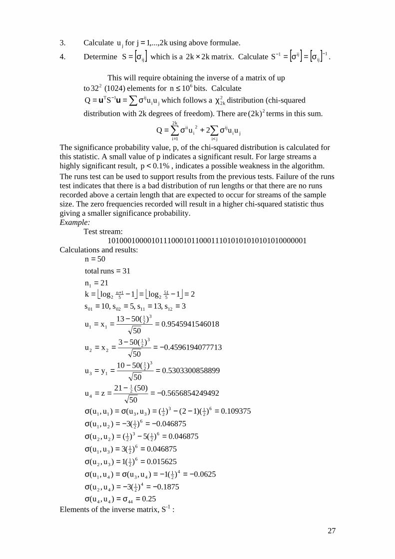
3. Calculate foru using above formulae. k2,...,1jj =

4. Determine [S = which is a ]ijσ k2k2 matrix. Calculate .

× [ ] [ ] 1ij

ij1S −− σ=σ=

This will require obtaining the inverse of a matrix of up to 32 elements for bits. Calculate

which follows a distribution (chi-squared

distribution with 2k degrees of freedom). There are terms in this sum.

)1024(2

== −1TS uu

610n ≤

∑σ jiij uuQ 2

k2χ2)k2(

∑ ∑= <

σ+σ=k2

1i jiji

ij2i

ii uu2uQ

The significance probability value, p, of the chi-squared distribution is calculated for this statistic. A small value of p indicates a significant result. For large streams a highly significant result, , indicates a possible weakness in the algorithm. %1.0p <The runs test can be used to support results from the previous tests. Failure of the runs test indicates that there is a bad distribution of run lengths or that there are no runs recorded above a certain length that are expected to occur for streams of the sample size. The zero frequencies recorded will result in a higher chi-squared statistic thus giving a smaller significance probability. Example: Test stream: 10100010000101110001011000111010101010101010000001 Calculations and results:

21n

31runstotal50n

1 ==

=

21log1logk 551

251n

2 =−=−= + 3s,13s,5s,10s 12110201 ====

0189545941546.050

)(5013xu3

21

11 =−==

7134596194077.050

)(503xu3

21

22 −=−==

8995303300858.050

)(5010yu3

21

13 =−==

4925656854249.050

)50(21zu 21

4 −=−

==

109375.0))(12()()u,u()u,u( 6213

21

3311 =−−=σ=σ 046875.0)(3)u,u( 6

21

21 −=−=σ 046875.0)(5)()u,u( 6

213

21

22 =−=σ 046875.0)(3)u,u( 6

21

31 ==σ 015625.0)(1)u,u( 6

21

32 ==σ 0625.0)(1)u,u()u,u( 4

21

4341 −=−=σ=σ 1875.0)(3)u,u( 4

21

42 −=−=σ 25.0)u,u( 4444 =σ=σ

Elements of the inverse matrix, S-1 :

27

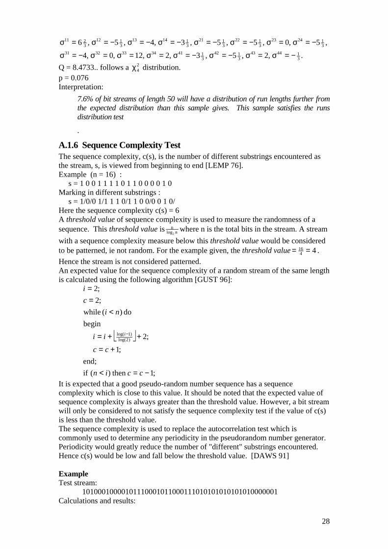
.,2,5,3,2,12,0,4

,5,0,5,5,3,4,5,6

314443

3142

314134333231

312423

3122

3121

311413

3112

3211

−=σ=σ−=σ−=σ=σ=σ=σ−=σ

−=σ=σ−=σ−=σ−=σ−=σ−=σ=σ

Q = 8.4733.. follows a distribution. 24χ

p = 0.076 Interpretation:

7.6% of bit streams of length 50 will have a distribution of run lengths further from the expected distribution than this sample gives. This sample satisfies the runs distribution test

.

A.1.6 Sequence Complexity Test The sequence complexity, c(s), is the number of different substrings encountered as the stream, s, is viewed from beginning to end [LEMP 76]. Example (n = 16) : s = 1 0 0 1 1 1 1 0 1 1 0 0 0 0 1 0 Marking in different substrings : s = 1/0/0 1/1 1 1 0/1 1 0 0/0 0 1 0/ Here the sequence complexity c(s) = 6 A threshold value of sequence complexity is used to measure the randomness of a sequence. This threshold value is nlog

n2

where n is the total bits in the stream. A stream with a sequence complexity measure below this threshold value would be considered to be patterned, ie not random. For the example given, the threshold value 44

16 == . Hence the stream is not considered patterned. An expected value for the sequence complexity of a random stream of the same length is calculated using the following algorithm [GUST 96]:

;1 then)( ifend;

;1

;2 begin

do )( while;2;2

)2log()1log(

−=<

+=

++=

<==

−

ccin

cc

ii

nici

i

It is expected that a good pseudo-random number sequence has a sequence complexity which is close to this value. It should be noted that the expected value of sequence complexity is always greater than the threshold value. However, a bit stream will only be considered to not satisfy the sequence complexity test if the value of c(s) is less than the threshold value. The sequence complexity is used to replace the autocorrelation test which is commonly used to determine any periodicity in the pseudorandom number generator. Periodicity would greatly reduce the number of "different" substrings encountered. Hence c(s) would be low and fall below the threshold value. [DAWS 91] Example Test stream: 10100010000101110001011000111010101010101010000001 Calculations and results:

28

13valueExpected859191.8valueThreshold

10)s(c50n

==

==

Interpretation: This sample stream is considered random based on the sequence complexity test.

A.1.7 Linear Complexity Test A.1.7.1 Linear Complexity The linear complexity test checks for the minimum amount of knowledge (bits) needed to reconstruct the whole stream. Every finite stream, s, can be produced by a linear feedback shift register (LFSR). The length of the shortest LFSR which will produce the stream is said to be the linear complexity of the stream, which will be denoted by L(s). If the value of L(s) is L then 2L consecutive terms can be used to reconstruct the whole sequence using the Berlekamp Massey algorithm. [MASS 69] Hence, in order to avoid stream reconstruction, the value of L should be large. Example: 01011001010100100111100000110111001100011101011111101101 This shortest recurrence relation which will create this sequence is: )()1()4()5()6( tututututu ⊕+⊕+⊕+=+where ⊕ is addition mod 2, and the first bit is u(0). For example:

If 0=t then . 01100

)0()1()4()5()6(⊕⊕⊕=

⊕⊕⊕= uuuuu

If 1=t then . 10001

)1()2()5()6()7(⊕⊕⊕=

⊕⊕⊕= uuuuu

If 2=t then . 01010

)2()3()6()7()8(⊕⊕⊕=

⊕⊕⊕= uuuuu

This means that the linear complexity, L(s), of this sequence is six. If any twelve consecutive bits are known then the whole sequence can be reconstructed. [MASS 69] It should be noted that some keystreams can pass all the previous tests yet possess a very small linear complexity. An example of this is an m-sequence (see [RUEP 84]). An m-sequence has a period of length and a linear complexity of L. An m-sequence has the best possible distribution of zeros and ones for a sequence of period . In this fashion an m-sequence appears to be statistically random in terms of tests A.1.1 to A.1.6. In fact m-sequences are commonly used as white noise generators. However, in terms of their use in a stream cipher an m-sequence offers very low security. Knowledge of only 2L consecutive bits of the keystream is needed to derive the defining LFSR and hence determine the whole keystream.

12L −

12L −

For large n, L(s) is approximately normally distributed with 81862

2n , =σ=µ [RUEP

84], [KREY 81]. Using the standardised normal statistic ))(( 28681 nsL −=z the

significance probability value, p, of the normal distribution is calculated. Since only low values of L(s) signify a possible weakness to the cipher, only a one-tailed test (lower tail) need apply. A small value of p indicates a significant result. For large streams a highly significant result ( ) indicates a possible weakness in the algorithm.

%1.0p <

29

The linear complexity test by itself can classify as random, streams which may be highly patterned, or contain large substrings which are highly patterned. Some of the previous test results should support this. e.g. a stream of 12

n − zeros followed by a one, and then followed by a repetition of these 2

n terms, has a linear complexity of 2n .

This stream would be classified as being random using the linear complexity test. Clearly, such a stream is highly patterned and would not satisfy the previous tests. However, it is possible to construct a stream of length n which would pass all the previous statistical tests, and have a linear complexity of approximately 2

n yet would contain a large highly patterned substring. Hence the following linear complexity profile tests are carried out. A.1.7.2 Linear Complexity Profile Since some highly patterned streams can give a linear complexity measure close to 2

n a second test measures the change in the linear complexity profile of the stream as each bit is added. Let s(i) be the substring formed by taking the first i bits of s. If L(s(i)) for i = 1,...,n denotes the linear complexity of s(i) then the values of s(i) are defined to be the linear complexity profile of s and should follow approximately the 2

i line [MASS 69]. A failure in this test would highlight any large deviations from the 2

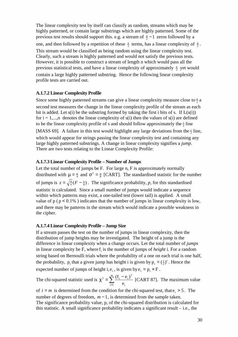
i line, which would appear for strings passing the linear complexity test and containing any large highly patterned substrings. A change in linear complexity signifies a jump. There are two tests relating to the Linear Complexity Profile: A.1.7.3 Linear Complexity Profile – Number of Jumps Let the total number of jumps be F. For large n, F is approximately normally distributed with 4

n=µ and 8n2 =σ [CART]. The standardised statistic for the number

of jumps is )( 48 nn Fz −=

%1.0p <

. The significance probability, p, for this standardised statistic is calculated. Since a small number of jumps would indicate a sequence within which patterns may exist, a one-tailed test (lower tail) is applied. A small value of p ( ) indicates that the number of jumps in linear complexity is low, and there may be patterns in the stream which would indicate a possible weakness in the cipher. A.1.7.4 Linear Complexity Profile – Jump Size If a stream passes the test on the number of jumps in linear complexity, then the distribution of jump heights may be investigated. The height of a jump is the difference in linear complexity when a change occurs. Let the total number of jumps in linear complexity be F, where is the number of jumps of height i. For a random string based on Bernoulli trials where the probability of a one on each trial is one half, the probability, that a given jump has height i is given by

if

ip i21

i )(p =Fi ×

. Hence the expected number of jumps of height i, , is given by . ie pei =

The chi-squared statistic used is ∑=

−=m

1i i

2ii2

e)ef(

1−

χ [CART 87]. The maximum value

of is determined from the condition for the chi-squared test, that . The number of degrees of freedom, m , is determined from the sample taken.

mi = 5ei >

The significance probability value, p, of the chi-squared distribution is calculated for this statistic. A small significance probability indicates a significant result – i.e., the

30

stream is considered to be non-random. For large samples a highly significant result, , indicates a possible weakness in the algorithm. %1.0p <

Example Test stream: 10100010000101110001011000111010101010101010000001 Calculations and results: Linear Complexity Test

81862

2

50

=

==

σµ n

n

5.0

0)25(

25)(

250

8681

==−=

=

pz

sL

Interpretation: 50 % of bit streams of length 50 will have a linear complexity less than this sample. This sample satisfies the linear complexity test.

Hence bits (the whole stream) is needed to reconstruct the stream using the Berlekamp-Massey algorithm.

50)(2 =× sL

Linear Complexity Profile - Number of jumps

8413.0

1)15(

15

450

508

==−=

=

pz

F

Interpretation: 84.13% of streams of length 50 will have a number of jumps in linear complexity less than this sample. This sample satisfies the test on the number of jumps in linear complexity.

Linear Complexity Profile – Jumps size .1,1,0,2,11 54321 ===== fffff

5.7e1 = Since for i , then these values are combined to give . The corresponding values of are combined to give .

5<ie 2>

if5.72 =+e

4f2 =+

0707.0

1121freedom of Degrees27.35.7

)5.74(5.7

)5.711(2 22

==−=−=

=+= −−

pm

χ

Interpretation: Approximately 7.07% of bit streams of length 50 will have a sump size distribution further from the expected distribution than this sample gives. The sample satisfies the test on the distribution of the linear complexity jump size.

31

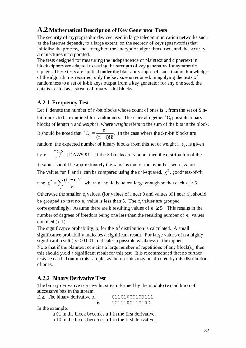
A.2 Mathematical Description of Key Generator Tests The security of cryptographic devices used in large telecommunication networks such as the Internet depends, to a large extent, on the secrecy of keys (passwords) that initialise the process, the strength of the encryption algorithms used, and the security architectures incorporated. The tests designed for measuring the independence of plaintext and ciphertext in block ciphers are adapted to testing the strength of key generators for symmetric ciphers. These tests are applied under the black-box approach such that no knowledge of the algorithm is required, only the key size is required. In applying the tests of randomness to a set of k-bit keys output from a key generator for any one seed, the data is treated as a stream of binary k-bit blocks.

A.2.1 Frequency Test Let denote the number of n-bit blocks whose count of ones is i, from the set of S n-bit blocks to be examined for randomness. There are altogether possible binary blocks of length n and weight i, where weight refers to the sum of the bits in the block.

if

in C

It should be noted that !i)!in(

!nCin

−= . In the case where the S n-bit blocks are

random, the expected number of binary blocks from this set of weight i, , is given

by

ie

ni

n

i 2SCe = [DAWS 91]. If the S blocks are random then the distribution of the

values should be approximately the same as that of the hypothesised values. if ieThe values for f and can be compared using the chi-squared, , goodness-of-fit

test:

i ie 2χ

∑=χk i

i2 e( −i

ef 2) where n should be taken large enough so that each ≥ 5.

Otherwise the smaller e values, (for values of i near 0 and values of i near n), should be grouped so that no e value is less than 5. The values are grouped correspondingly. Assume there are k resulting values of . This results in the number of degrees of freedom being one less than the resulting number of e values obtained (k-1).

ie

i

i

i if5ei ≥

The significance probability, p, for the distribution is calculated. A small significance probability indicates a significant result. For large values of n a highly significant result ( ) indicates a possible weakness in the cipher.

2χ

001.0<pNote that if the plaintext contains a large number of repetitions of any block(s), then this should yield a significant result for this test. It is recommended that no further tests be carried out on this sample, as their results may be affected by this distribution of ones.

A.2.2 Binary Derivative Test The binary derivative is a new bit stream formed by the modulo two addition of successive bits in the stream. E.g. The binary derivative of 01101000100111 is 1011100110100 In the example:

a 01 in the block becomes a 1 in the first derivative, a 10 in the block becomes a 1 in the first derivative,

32

a 00 in the block becomes a 0 in the first derivative, a 11 in the block becomes a 0 in the first derivative.

The frequency test is applied to the sample of binary derivative blocks. Parameters needed: S = number of blocks n-1 = length of binary derivative block (in bits) By taking the binary derivative of each of the S blocks to be examined, a set of S binary blocks of length n-1 are formed. Let f denote the number of these derivative blocks of hamming weight i, where hamming weight refers to the sum of the bit values in the block.

'i

There are altogether possible binary blocks of length n-1 and weight i. In the case where the S binary blocks are random, the expected number of binary blocks

from this sample of weight i, , is given by

i1n C−

'ie 1n

i1n

i 2SC

−

−

=e [DAWS 91].

If the S binary derivative blocks are random then the distribution of the values should be approximately the same as that of the hypothesised e values. The values for and e can be compared using the chi-squared, χ , goodness-of-fit test:

'if

'i

'if '

i2

∑χk

'i

2'i2 )e( −'i

ef= where n should be taken large enough so that each ≥ 5. '

ie

A similar interpretation to the frequency test is applied.

A.2.3 Subblock Test Subblocks of length b bits are chosen from each block. The user has the option to select the bit positions, or they may be randomly selected. There are four testing procedures for subblock lengths: b = 1, 2, 3 to 16, and greater than 16. b = 1: The key blocks will be tested for randomness in each of the n bit positions. The ith position, 1 ≤ i ≤ n, in each of the S blocks gives a stream of S bits to which a frequency test (as used for the stream cipher – see Section A.1.1) is applied. This determines weaknesses in any single bit position. Since the frequency test is highly sensitive to small deviations from the mean, the n results will not be combined to give an overall statistic for this test. A summary of results will be given, so that any problems with individual bit positions may be detected. For significance probabilities less than 0.001 in this test, it is highly unlikely that further subblock tests for b > 1 will give significant results when including any one of these bits. b = 2: For i ≠ j, 1 ≤ i ≤ n and 1 ≤ j ≤ n, a uniformity test with b = 2 is applied to each of the pairs of values in position i and j for each block. The test statistic used is 2

n C

∑=

3

0i

fS4 −=χ 2

i2 S , which follows a chi-squared distribution with three degrees of

freedom. This determines whether ciphertext bits i and j are independent or if a dependence exists between them. Since each bit position is used in more than one of the tests applied, the chi-squared statistics obtained are not independent, and so cannot be combined into one test statistic. A summary of significance probabilities will be given.

2n C

b ≥ 3: The tests applied to subblocks of length greater than three are the same as for the stream cipher subblock tests (see Section A.1.4), i.e. if b ≤ 16 then a test of uniformity is applied, whereas if b > 16 the repetition test is applied.

33

A.2.4 Block Entropy The number of independent bits in the block is calculated, using the application of the repetition test (see Section A.1.4), to estimate the entropy of the block. Method of calculating entropy: Using the results of the repetition test, a 99% probability interval for the mean number of block (or subblock) repetitions, λ, that the cipher could generate in a sample of size S where r5758.2r ±=λ , is given by applying a normal approximation to the Poisson distribution. This is used to find a 99% probability interval for the size of the population, N, of blocks (or subblocks) that could be generated by such a cipher, using λ= 2

S2

N =

N [DAWS 98]. Since the total number of binary patterns for a block/subblock of B bits is , then the number of independent bits, H, is estimated from a table of values . The values of H (or in the case of subblocks, H

B2H2 i)

corresponding to the end points of the probability interval for N give a probabilistic interval for the entropy of the block (or subblock). If the number of repetitions is found to be greater than 48 (approximately three standard deviations above the mean) for a sample of less than 32

B +2 blocks (B = block/subblock size) then the cipher is considered to generate non-random data. A message will be given in such cases. The results will give the estimate of block entropy. If subblocks are used, then a table of entropy estimates for the subblocks will also be included. If the entropy is less than the block size, then the reduction indicates the number of dependent bits in the block. If the entropy of the whole block was calculated then a 99% probability interval for the true entropy of the block, H, is given. If the block has been divided into k subblocks, then the block entropy, H, is estimated by the bounds

where the lower bound is the maximum subblock entropy and

holds with a probability of 0.995, and the upper bound is the sum of the k subblock entropies and holds with a probability of

∑=

≤≤k

1iii HH)H(Max

k995.0 .If the sample of blocks gives at least 20 repetitions, then the block entropy is estimated. In the case where the number of blocks is greater than 32 +n

2 then the estimate for block entropy will be given using no more than 2 blocks. If the number of repetitions is less than 20, then a whole block estimate will not be given, and instead, a bound for the entropy is calculated by combining entropy estimates from smaller subblocks. In this case the block is divided into subblocks of length B, where the maximum length, B, of the subblocks is determined from the number of blocks to be tested, S, such that

3−n

32B

2S += . Any remaining bits, d, are tested using a sample of 32

d

2 +=s subblocks of d bits (d < B) from these positions in each block. If d ≤ 16 then the requirements of the repetition test are not satisfied. In this case the entropy of the subblock is taken as d, the subblock size. The entropy is estimated for each subblock, as long as the number of subblock repetitions is at least 20. If the number of repetitions is less than 20 then the entropy estimate cannot be assumed to be any less than the length of the subblock. These estimates are then added to give an upper bound for the whole block entropy. The best application of this estimation is applied to samples of approximately 32

B +2 sublocks of length B bits, where B > 16 and for which the expected number of repetitions is 32. The following table gives the entropy estimate for a sample of one

34

million blocks, when the number of repetitions is 30, 50 or 100. It should be noted that this is independent of the block size used.

Repetitions Entropy estimate 30 34 50 33 100 35

In the case when 30 repetitions occur, the minimum sample size, S, required to obtain a 0.99 probability interval for the block entropy, H, that includes the actual block size, is given in the table below. If 30 repetitions occurred in a smaller sample, or more than 30 repetitions occurred in a sample of the same size, then the block entropy would be lowered.

Actual key size 0.99 probability interval for H Sample size required, S 32 31.5 – 32 3.7 × 105 40 38.5 – 40 6.0 × 106 56 54.5 – 56 1.5 × 109 64 62.5 – 64 2.4 × 1010 80 78.5 – 80 6.2 × 1012 128 126.5 – 128 1.04 × 1020

35

A.3 Bibliography

[BEKE 82] H. Beker and F.Piper, Cipher Systems: The Protection of Communications, Northwood Books, London, 1982.

[BHAT 77] G. Bhattacharyya and R. Johnson, Statistical Concepts and Methods, John Wiley & Sons, 1977.

[CARR 88] J.M. Carroll and L.E. Robbins, “Using binary derivatives to test an enhancement of DES”, Cryptologia, Vo1 12 number 4, 1988, pp 193-208.

[CART 87] G. Carter, “A statistical test for randomness based on the linear complexity profile of a binary sequence”, Technical Report for Racal Comsec Ltd., 1987.

[DAWS 91] E.P. Dawson, Design and Cryptanalysis of Symmetric Ciphers, PhD Thesis, Queensland University of Technology, 1991.

[DAWS 98] E.P. Dawson and H.M. Gustafson, “A Method for measuring Entropy of Symmetric Cipher Key Generators”, Computers and Security, Vol. 17 No. 2, pp 177 - 184, 1998.

[DIFF 79] W. Diffie and M.E. Hellman, “Privacy and Authentication: An Introduction to Cryptography”, Proceedings of the IEEE, Vol. 67, No. 3, March 1979, pp 397-427.

[FOLK 84] L.J. Folks, “Combination of Independent Tests”, Handbook of Statistics, Vol. 4, Elsevier Science Publishers, 1984, pp 113-121.

[GUST 96] H.M. Gustafson, Statistical Analysis of Symmetric Ciphers, PhD Thesis, Queensland University of Technology, Brisbane Australia, 1996.

[KOLC 66] V.F. Kolchin, “The Speed of Convergence to Limit Distributions in The Classical Ball Problem”, Theory of Probability and its Applications, 11, 1966, 128-140.

[KREY 81] E. Kreysig, Introductory Mathematical Statistics, John Wiley and Sons, 1981.

[LEMP 76] A. Lempel and J. Ziv, “On the complexity of finite sequences”, IEEE Trans. on Information Theory, Vol.IT-22, Jan.1976,pp 75-81.

[MASS 69] J.L. Massey, “Shift register sequences and BCH decoding”, IEEE Transactions on Information Theory, Vol. IT-15, Jan. 1969, pp 122-127.

[MAUR 92] U.M. Maurer, “A Universal Statistical Test for Random Bit Generators”, Journal of Cryptology, 1992, 5, pp 89-105.

[MARS 84] G. Marsaglia, “A Current View of random Number Generators”, Proceedings of the Sixteenth Symposium on the Interface, Computer Science and Statistics, Editor L. Billard, Elsevier Science Publishers, 1984. pp3 - 10.

[MASS 69] J.L. Massey, “Shift Register Sequences and BGH Decoding”, IEEE Trans. on Information Theory, Vol. IT-15, Jan. 1969, pp 122-127.

[MOOD 40] A.M. Mood, “The distribution theory of runs”, Ann. Math. Statist., Vol 11, 1940, pp 367-392.

[PETT 79] A.N. Pettitt, “A non-parametric approach to the change - point problem”, Appl. Statist., Vol. 28 No. 2, 1979, pp 126-135.

[RUEP1 84] R.A. Rueppel, New Approaches to Stream Ciphers, PhD Thesis, Swiss Federal Institute of Technology, 1984.

36

[RUEP2 84] R.A. Reuppel, “Analysis and Design of Stream Ciphers”, Springer-Verlag, 1986.

[STEP 86] M.A. Stephens and R.B. D'Agostino, “Tests based on EDF Statistics”, Goodness of Fit Techniques, in Statistics, Textbooks and Monographs; Vol. 68, Marcel Dekker Inc., 1986, pp 97-193.

[WEBS 86] A.E. Webster and S.E. Tavares, “On the Design of S-Boxes”, Advances in Cryptology: Crypto' 85, Springer-Verlag, 1986, pp. 523-530.

37

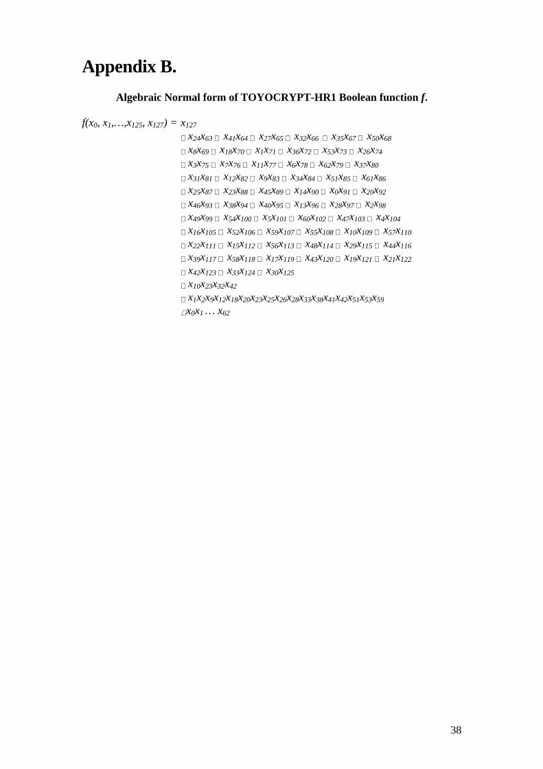
Appendix B.

Algebraic Normal form of TOYOCRYPT-HR1 Boolean function f. f(x0, x1,…,x125, x127) = x127

⊕ x24x63 ⊕ x41x64 ⊕ x27x65 ⊕ x32x66 ⊕ x35x67 ⊕ x50x68 ⊕ x8x69 ⊕ x18x70 ⊕ x1x71 ⊕ x36x72 ⊕ x53x73 ⊕ x26x74 ⊕ x3x75 ⊕ x7x76 ⊕ x11x77 ⊕ x6x78 ⊕ x62x79 ⊕ x37x80 ⊕ x31x81 ⊕ x12x82 ⊕ x9x83 ⊕ x34x84 ⊕ x51x85 ⊕ x61x86 ⊕ x25x87 ⊕ x23x88 ⊕ x45x89 ⊕ x14x90 ⊕ x0x91 ⊕ x20x92 ⊕ x46x93 ⊕ x38x94 ⊕ x40x95 ⊕ x13x96 ⊕ x28x97 ⊕ x2x98 ⊕ x49x99 ⊕ x54x100 ⊕ x5x101 ⊕ x60x102 ⊕ x47x103 ⊕ x4x104 ⊕ x16x105 ⊕ x52x106 ⊕ x59x107 ⊕ x55x108 ⊕ x10x109 ⊕ x57x110 ⊕ x22x111 ⊕ x15x112 ⊕ x56x113 ⊕ x48x114 ⊕ x29x115 ⊕ x44x116 ⊕ x39x117 ⊕ x58x118 ⊕ x17x119 ⊕ x43x120 ⊕ x19x121 ⊕ x21x122 ⊕ x42x123 ⊕ x33x124 ⊕ x30x125 ⊕ x10x23x32x42

⊕ x1x2x9x12x18x20x23x25x26x28x33x38x41x42x51x53x59

⊕ x0x1 … x62

38

Appendix C.

Sorted input differences for quadratic terms – TOYOCRYPT-HR1 Index for first factor Index for second factor Difference 62 79 17 50 68 18 53 73 20 41 64 23 61 86 25 35 67 32 32 66 34 51 85 34 36 72 36 27 65 38 24 63 39 60 102 42 37 80 43 45 89 44 54 100 46 46 93 47 26 74 48 59 107 48 31 81 50 34 84 50 49 99 50 18 70 52 55 108 53 57 110 53 52 106 54 40 95 55 38 94 56 47 103 56 56 113 57 58 118 60 8 69 61 25 87 62 23 88 65 11 77 66 48 114 66 7 76 69 28 97 69 1 71 70 12 82 70 3 75 72 6 78 72 20 92 72 44 116 72 9 83 74 14 90 76

39

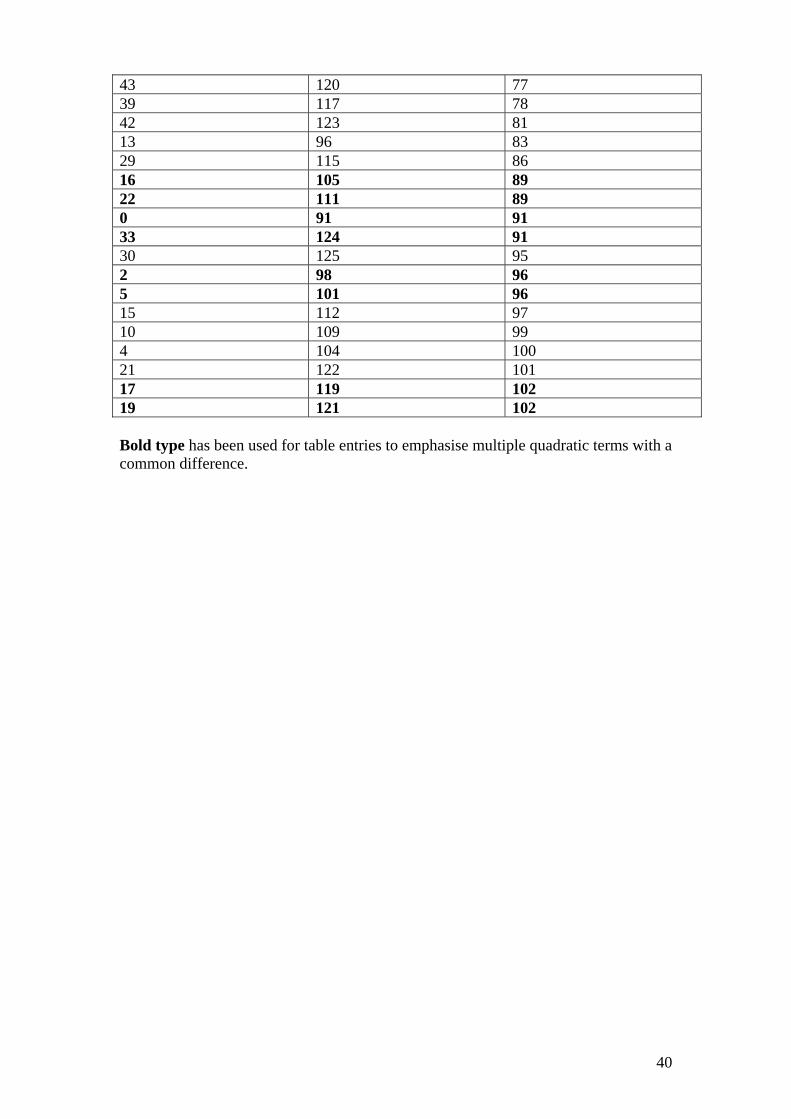
43 120 77 39 117 78 42 123 81 13 96 83 29 115 86 16 105 89 22 111 89 0 91 91 33 124 91 30 125 95 2 98 96 5 101 96 15 112 97 10 109 99 4 104 100 21 122 101 17 119 102 19 121 102 Bold type has been used for table entries to emphasise multiple quadratic terms with a common difference.

40

Appendix D. Results of Linear Complexity Tests on TOYOCRYPT-HR1 Length of output stream = 1,000,000 bits. Number of streams = 10 Test Key1 Key2 Key3 Key4 Key5 Key6 Key7 Key8 Key9 KeyaLinear Complexity 4999

98 499998

500002

500001

500000

500000

499999

500000

500000

500000

LC p-value .0261 .0261 .9739 .8341 .5000 .5000 .1659 .5000 .5000 .5000LC - Jumps .2623 .5113 .2965 .1926 .4050 .3429 .0812 .5214 .2415 .8261LC - Jump Size .7099 .6622 .3050 .6306 .8919 .6059 .1111 .7357 .0931 .0269

41

Appendix E. Results of CRYPT-X Tests on TOYOCRYPT-HR1 Length of output stream = 10,000,000 bits. Length of output stream = 1,000,000 bits. (Sequence Complexity Test) Number of streams = 10 Test Key1 Key2 Key3 Key4 Key5 Key6 Key7 Key8 Key9 KeyaFrequency .6561 .6557 .6557 .6557 .6552 .6557 .1705 .6833 .5858 .0163Binary Derivative (1) .2094 .2092 .2090 .2090 .2090 .2088 .1675 .8527 .8064 .1070Binary Derivative (2) .1034 .1033 .1033 .1033 .1033 .1034 .1970 .9728 .9496 .4803Change Point .5793 .5994 .5790 .5787 .5787 .5787 .0833 .2228 .0930 .7717Subblock b = 2 .3439 .9706 .3434 .9706 .3429 .9705 .3290 .1736 .6109 .0971Subblock b = 3 .0185 .0604 .0826 .0185 .0603 .0826 .0300 .2895 .7957 .1030Subblock b = 4 .6667 .2959 .1012 .2760 .6656 .2955 .7999 .1191 .1647 .0772Subblock b = 5 .7335 .4502 .4864 .1967 .4876 .7332 .3051 .3836 .4255 .3310Subblock b = 6 .0859 .0020 .0412 .0978 .5439 .7844 .4027 .8225 .6383 .4330Subblock b = 7 .5260 .1514 .3687 .9734 .4454 .4265 .8331 .3242 .8283 .5846Subblock b = 8 .4062 .4001 .1335 .1879 .1365 .0177 .1423 .2726 .3422 .0840Subblock b = 9 .6126 .1129 .0659 .0882 .3296 .5648 .7061 .0562 .9982 .8099Subblock b = 10 .6075 .0945 .2173 .2728 .3865 .5614 .3586 .6457 .0902 .0264Subblock b = 11 .4800 .2656 .1368 .4871 .3414 .2927 .4013 .0724 .3623 .1006Subblock b = 12 .0358 .3106 .2596 .0389 .7884 .0069 .6168 .2688 .6880 .9286Subblock b = 13 .2134 .8827 .6305 .1608 .3686 .9117 .7010 .4549 .6942 .8530Subblock b = 14 .6850 .6993 .2170 .7144 .8451 .9438 .7418 .2320 .4656 .9309Subblock b = 15 .4584 .6548 .6577 .2402 .0536 .0607 .0451 .9187 .3087 .4361Subblock b = 16 .0252 .0083 .0007 .1570 .7279 .5014 .1228 .6901 .7545 .3233Subblock b = 17 .0047 .2159 .5959 .7237 .4795 .4795 .1116 .2888 .1116 .2888Subblock b = 18 .4795 .4795 .4795 .8597 .2888 .5959 .8597 .1116 .3768 .0771Subblock b = 19 .8597 .5959 1.000 .3768 .3768 .0518 .0518 .5959 .8597 .0339Subblock b = 20 .3768 .4795 .5959 .3768 .4795 .8597 .8597 .2159 .8597 .0216Subblock b = 21 .5959 .4795 .2888 .4795 .2159 .2888 .2159 .7237 .1573 .3768Subblock b = 22 1.000 .1573 .4795 .7237 .7237 1.000 1.000 .0771 .1573 .2888Subblock b = 23 .2888 .1116 .1116 .1573 .3768 .4795 .2888 .0399 .2159 .7237Subblock b = 24 1.000 .3768 .0518 .3768 .8597 .8597 .2888 .8597 .4795 .8597Subblock b = 25 .4795 .1116 .3768 .2888 .1573 .5959 .2159 .4795 .4795 .8597Subblock b = 26 .1116 .7237 .0771 .5959 .8597 .5959 .0027 .4795 1.000 .1573Subblock b = 27 .4795 .8597 .1573 .7237 .8597 .5959 1.000 1.000 .3768 .4795Subblock b = 28 .4795 .4795 .1573 .8597 .4795 .5959 .4795 .5959 1.000 1.000Subblock b = 29 .4795 .5959 .8597 .2888 .0339 .0771 .3768 .1116 .7237 .8597Subblock b = 30 .1116 .0771 .3768 .7237 1.000 .2888 .8597 .3768 .2159 .1116Runs Distribution .8082 .8084 .8083 .8083 .8084 .8086 .6265 .1958 .8627 .7661Longest Run Length 25 25 25 25 25 25 21 23 24 23 Sequence Complexity 5079

5 50795

50794

50795

50794

50795

50829

50771

50799

50742

Sequence Complexity: Threshold value = 50,441 Mean value = 50172 Session Keys Used (HEX): 1: 00000000000000000000000000000001 2: 00000000000000000000000000000002 3: 00000000000000000000000000000004 4: 00000000000000000000000000000008 5: 00000000000000000000000000000010 6: 00000000000000000000000000000020 7: 38b3c50fd5b1bccc49e786ebf28f5a51 8: 04b81a3a854e38b6775cbf4caeb4f1e5 9: f2a09ae954cda165661efc765aeeb0c3 a: 9f9e5ded6e10cfa557c1fe0ed02f1f3f Fixed key (in HEX): ecb91d4ce0badb56023ca06869e92a2f

42

Appendix F.

Results of Entropy Tests Distribution of Subblocks Length of output stream = 1 Gigabyte Number of streams = 1

p-value Subblock size Ones Runs

40 .1772 .299848 .3579 .155456 .0300 .934764 .2233 .7193

128 .4774 .9479256 .0700 .7785512 .5697 .2228

1024 .9494 .5528

43