EVALUATION OF THE PERFORMANCE AND AIR POLLUTANT EMISSIONS ...€¦ · The evaluation of the...

E n e r g y R e s e a r c h a n d De v e l o p m e n t Di v i s i o n F I N A L P R O J E C T R E P O R T

EVALUATION OF THE PERFORMANCE AND AIR POLLUTANT EMISSIONS OF HEAVY-DUTY VEHICLES OPERATING ON VARIOUS NATURAL GAS BLENDS

MARCH 2015 CEC-500 -2016-029

Prepared for: California Energy Commission Prepared by: University of California, Riverside

Prepared by: Primary Author(s): Georgios Karavalakis Thomas D. Durbin Kent C. Johnson Maryam Hajbabaei CE-CERT University of California, Riverside 1084 Columbia Ave., Riverside, CA 92507 Tel : 951-781-5791 Fax : 951-781-5790 Contract Number: 500-12-009 Prepared for: California Energy Commission Matthew Fung Contract Manager

Aleecia Gutierrez Office Manager Energy Generation Research Office

Laurie ten Hope Deputy Director RESEARCH AND DEVELOPMENT DIVISION

Robert P. Oglesby

Executive Director

DISCLAIMER

This report was prepared as the result of work sponsored by the California Energy Commission. It does not necessarily represent the views of the Energy Commission, its employees or the State of California. The Energy Commission, the State of California, its employees, contractors and subcontractors make no warrant, express or implied, and assume no legal liability for the information in this report; nor does any party represent that the uses of this information will not infringe upon privately owned rights. This report has not been approved or disapproved by the California Energy Commission nor has the California Energy Commission passed upon the accuracy or adequacy of the information in this report.

iii

ACKNOWLEDGEMENTS

The authors would like to thank the following organizations and individuals for their valuable

contributions to this project:

We acknowledge funding from the California Energy Commission under contract 500-12-009.

Additional funding for this contract was also provided by the California Air Resources Board

under contract 12-412.

We also acknowledge the Colton Unified school district for providing the school bus and the

Waste Management company for providing the waste hauler truck.

We acknowledge Mr. Don Pacocha, Mr. Eddie O’Neal, and Mr. Joe Valdez, of the University of

California, Riverside for their contributions in conducting the emissions testing for this

program.

iv

PREFACE

The California Energy Commission Public Interest Energy Research (PIER) Program supports

public interest energy research and development that will help improve the quality of life in

California by bringing environmentally safe, affordable, and reliable energy services and

products to the marketplace.

The PIER Program conducts public interest research, development, and demonstration (RD&D)

projects to benefit California.

The PIER Program strives to conduct the most promising public interest energy research by

partnering with RD&D entities, including individuals, businesses, utilities, and public or

private research institutions.

PIER funding efforts are focused on the following RD&D program areas:

Buildings End-Use Energy Efficiency

Energy Innovations Small Grants

Energy-Related Environmental Research

Energy Systems Integration

Environmentally Preferred Advanced Generation

Industrial/Agricultural/Water End-Use Energy Efficiency

Renewable Energy Technologies

Transportation

Impact of Natural Gas Composition on the Performance & Emissions of Heavy -Duty Natural

Gas Vehicles - Phase 2 is the final report for the Impact of Natural Gas Composition on the

Performance & Emissions of Heavy-Duty Natural Gas Vehicles - Phase 2 project

(contract number 500-12-009) conducted by CE-CERT, University of California, Riverside. The

information from this project contributes to PIER’s Energy-Related Environmentally Research

Program.

For more information about the PIER Program, please visit the Energy Commission’s website at

www.energy.ca.gov/research/ or contact the Energy Commission at 916-654-4878.

http://www.energy.ca.gov/research/

v

ABSTRACT

Natural gas composition can have an important impact on natural gas vehicle emissions and

performance. With the expansion of natural gas production methods, a wider range of natural

gas composition is available for use throughout California. This study’s objective was to

evaluate the natural gas composition impact on the performance and emissions of 2005 to 2013

heavy-duty vehicle models. A natural gas school bus, a natural gas waste hauler, a Class 8

natural gas refuse truck, and two Class 8 natural gas port trucks were selected and tested over

application-specific duty cycles for 22 vehicle test days. The researchers conducted tests using a

heavy-duty chassis dynamometer—a device used for measuring emissions and performance—

with a range of three to seven different test fuels. Each fuel test compared exhaust emissions,

fuel economy, particulate matter mass, particle number and particle size distributions, ammonia

emissions, carbonyl compound emissions, and nitrous oxide emissions. The researchers found

that the lean-burn school bus engine produced more pollutants compared to the stoichiometric

waste hauler and port trucks. The stoichiometric engines also showed considerably lower

emissions compared to previous studies of lean-burn technology. Using the low methane fuels,

the lean-burn school bus and the local-haul tested port truck showed increases in pollutant

emissions. The waste hauler and near-dock port truck showed mixed results with the low

methane fuels. The evaluation of the performance and air pollutant emissions of heavy-duty

vehicles operating on various natural gas blends ultimately benefits the understanding of gas

interchangeability to ensure optimal vehicle performance and reduction of greenhouse gasses.

Keywords: Natural Gas, Vehicle Emissions, Transportation, Alternative Fuels

Please use the following citation for this report:

Karavalakis, Georgios, Durbin, Thomas D., Johnson, Kent C., and Hajbabaei, Maryam

(University of California, Riverside). 2016. Evaluation of the Performance and Air Pollutant

Emissions of Heavy-Duty Vehicles Operating on Various Natural Gas Blends , California

Energy Commission. Publication number: CEC-500-2016-029.

vi

TABLE OF CONTENTS

Acknowledgements ................................................................................................................................ iii

PREFACE ................................................................................................................................................... iv

ABSTRACT ................................................................................................................................................ v

TABLE OF CONTENTS .......................................................................................................................... vi

EXECUTIVE SUMMARY ...................................................................................................................... 12

Introduction .................................................................................................................................... 12

Project Purpose and Process ......................................................................................................... 12

Project Results ................................................................................................................................. 13

Project Benefits................................................................................................................................ 14

CHAPTER 1: Introduction .................................................................................................................... 16

CHAPTER 2: Experimental Procedures .............................................................................................. 19

2.1 Test Fuels ......................................................................................................................................... 19

2.1.1 Fuel Composition and Rich and Lean Combustion .................................................... 20

2.2 Test Vehicles.................................................................................................................................... 21

2.3 Test Cycles ....................................................................................................................................... 22

2.4 Emissions Testing and Measurements ........................................................................................ 27

CHAPTER 3: Heavy-Duty Vehicle Chassis Dynamometer Testing Results ............................... 31

3.1 Nitrogen Oxides Emissions .......................................................................................................... 31

3.2 Total Hydrocarbon Emissions ...................................................................................................... 37

3.3 Nonmethane Hydrocarbon Emissions ........................................................................................ 43

3.4 Methane Emissions ........................................................................................................................ 49

3.5 Carbon Monoxide Emissions ........................................................................................................ 55

3.6 Fuel Economy and Carbon Dioxide Emissions .......................................................................... 61

3.7 Particulate Matter Mass Emissions .............................................................................................. 76

3.8 Particle Number Emissions ........................................................................................................... 80

3.9 Particle Size Distributions ............................................................................................................. 86

3.10 Ammonia Emissions .................................................................................................................... 92

vii

3.11 Carbonyl Emissions ................................................................................................................. 99

3.12 Nitrous Oxide Emissions ...................................................................................................... 106

CHAPTER 4: Summary ........................................................................................................................ 111

4.1 2005 John Deere School Bus ........................................................................................................ 111

4.2 2011 Cummins Westport ISL G Waste Hauler ......................................................................... 112

4.3 2012 Cummins Westport ISL G Truck ....................................................................................... 112

4.4 2013 Cummins Westport ISX12 G .............................................................................................. 112

4.5 General ........................................................................................................................................... 113

CHAPTER 5: Conclusions and Recommendations ........................................................................ 114

GLOSSARY ............................................................................................................................................ 115

REFERENCES ........................................................................................................................................ 117

APPENDIX A: Engine Certification value ...................................................................................... A-1

APPENDIX B. Emissions Test Results .............................................................................................. B-1

APPENDIX C : Fuel Economy/Consumption Calculation ............................................................ C-1

LIST OF FIGURES

Figure 1: Double CBD Cycle with Warm-up........................................................................................ 24

Figure 2: Refuse Truck Cycle .................................................................................................................. 25

Figure 3: Near Dock Duty Cycle ............................................................................................................ 26

Figure 4: Local Haul Duty Cycle ............................................................................................................ 26

Figure 5: Typical Setup of Test Vehicles on the Chassis Dynamometer .......................................... 28

Figure 6: Schematic of the Sampling Systems and Instruments ........................................................ 30

Figure 7: Average NOx Emissions for the John Deere Bus ................................................................ 32

Figure 8 (a-b): Average NOx Emissions for the Waste Hauler Transport and Curbside Segments

............................................................................................................................................................ 33

Figure 9: Average NOx Emissions for the Waste Hauler for the Compaction Segment on an

Engine bhp-hr Basis ........................................................................................................................ 34

Figure 10: NOx Emissions for the Class 8 Trucks Cummins Westport ISL G Over the Near Dock

Cycle (A) and Cummins Westport ISX12 G Over the Local Haul Duty Cycle (B) for Their

Individual Phases ............................................................................................................................ 36

viii

Figure 11: Average THC Emissions for the John Deere Bus .............................................................. 38

Figure 12 (a-b): Average THC Emissions for Waste Hauler Transport and Curbside Segments . 39

Figure 13: Average THC Emissions for the Waste Hauler for the Compaction and on an Engine

bhp-hr Basis ...................................................................................................................................... 40

Figure 14: THC Emissions for the Class 8 Trucks Cummins Westport ISL G Over the Near Dock



Figure 15: Average NMHC Emissions for the John Deere Bus ......................................................... 44

Figure 16 (a-b): Average NMHC Emissions for Waste Hauler Transport and Curbside Segments

............................................................................................................................................................ 45

Figure 17: Average NMHC Emissions for Waste Hauler for the Compaction Segment on an


Figure 18: NMHC Emissions for the Class 8 Trucks Cummins Westport ISL G Over the Near

Dock Cycle (A) and Cummins Westport ISX12 G Over the Local Haul Duty Cycle (B) for

Their Individual Phases .................................................................................................................. 48

Figure 19: Average CH4 Emissions for the John Deere Bus ............................................................... 50

Figure 20 (a-b): Average CH4 Emissions for Waste Hauler Transport and Curbside Segments .. 51

Figure 21: Average CH4 Emissions for Waste Hauler for the Compaction Segment on an Engine

bhp-hr Basis ...................................................................................................................................... 52

Figure 22: CH4 Emissions for the Class 8 Trucks Cummins Westport ISL G Over the Near Dock



Figure 23: Average CO Emissions for the John Deere Bus ................................................................. 55

Figure 24 (a-b): Average CO Emissions for Waste Hauler Transport and Curbside Segments ... 57

Figure 25: Average CO Emissions for Waste Hauler for the Compaction Segment on an Engine

bhp-hr Basis ...................................................................................................................................... 58

Figure 26: CO Emissions for the Class 8 Trucks Cummins Westport ISL G Over the Near Dock



Figure 27: Average Volumetric Fuel Economy for the John Deere Bus ........................................... 62

Figure 28: Average Energy Equivalent Fuel Economy for the John Deere Bus .............................. 63

Figure 29 (a-b): Average Volumetric Fuel Economy for the Waste Hauler Transport and

Curbside Segments .......................................................................................................................... 65

ix

Figure 30: Average Volumetric Fuel Consumption for the Waste Hauler for the Compaction

Segment on an Engine bhp-hr Basis ............................................................................................. 66

Figure 31 (a-b): Average Energy Equivalent Fuel Economy for the Waste Hauler Transport and

Curbside Segments .......................................................................................................................... 67

Figure 32: Average Energy Equivalent Fuel Consumption for the Waste Hauler for the

Compaction Segment on an Engine bhp-hr Basis ....................................................................... 68

Figure 33: Volumetric Fuel Economy for the Class 8 Trucks Cummins Westport ISL G Over the

Near Dock Cycle (A) and Cummins Westport ISX12 G Over the Local Haul Duty Cycle (B)

for Their Individual Phases ............................................................................................................ 70

Figure 34: Energy Equivalent Fuel Consumption for the Class 8 Trucks Cummins Westport ISL

G Over the Near Dock Cycle (A) and Cummins Westport ISX12 G Over the Local Haul

Duty Cycle (B) for Their Individual Phases ................................................................................. 71

Figure 35: Average CO2 Emissions for the John Deere Bus ............................................................... 72

Figure 36 (a-b): Average CO2 Emissions for the Waste Hauler Transport and Curbside Segments

............................................................................................................................................................ 73

Figure 37: Average CO2 Emissions for the Compaction Segment of the Waste Hauler on an


Figure 38: CO2 Emissions for the Class 8 Trucks Cummins Westport ISL G Over the Near Dock



Figure 39: Average PM Emissions for the John Deere Bus ................................................................ 77

Figure 40: Average PM Emissions for the Waste Hauler ................................................................... 79

Figure 41: PM Mass Emissions for the Class 8 Trucks Cummins Westport ISL G Over the Near

Dock Cycle (A) and Cummins Westport ISX12 G Over the Local Haul Duty Cycle (B)....... 80

Figure 42: Average PN Emissions for the John Deere Bus ................................................................. 81

Figure 43: Average PN Emissions for Waste Hauler .......................................................................... 83

Figure 44: Average PN Emissions for Waste Hauler .......................................................................... 84

Figure 45: PN Emissions for the Cummins Westport ISL-G Truck (Near Dock Cycle) ................. 85

Figure 46: PN Emissions for the Cummins Westport ISLX12G Truck ............................................. 86

Figure 47: Average Particle Size Distributions for the John Deere Bus ............................................ 87

Figure 48: Average Particle Size Distributions for the Waste Hauler ............................................... 89

Figure 49: Average Particle Size Distributions for the Cummins Westport ISL-G Truck ............. 90

x

Figure 50: Particle Size Distributions for the Cummins Westport ISX12G Truck .......................... 92

Figure 51: Average NH3 Emissions for the John Deere Bus ............................................................... 94

Figure 52 (a-b): Average NH3 Emissions for Waste Hauler Transport and Curbside Segments.. 96

Figure 53: Average NH3 Emissions for Waste Hauler for the Compaction Segment on an Engine

bhp-hr Basis ...................................................................................................................................... 97

Figure 54: NH3 Emissions for the Cummins Westport ISL G (A) and Cummins Westport ISX12

G (B) Class 8 Trucks Over the Near Dock Cycle and the Local Haul Duty Cycle ................. 99

Figure 55: Average Formaldehyde Emissions for the John Deere Bus ........................................... 101

Figure 56: Average Acetaldehyde Emissions for the John Deere Bus ............................................ 102

Figure 57: Average Formaldehyde Emissions for Waste Hauler .................................................... 103

Figure 58: Average Acetaldehyde Emissions for Waste Hauler Truck .......................................... 104

Figure 59: Formaldehyde and Acetaldehyde Emissions for the Cummins Westport ISL G (A)

and Cummins Westport ISX12 G (B) Class 8 Trucks Over the Near Dock Cycle and the

Local Haul Duty Cycle ................................................................................................................. 105

Figure 60: N2O Emissions for the John Deere Bus ............................................................................. 107

Figure 61: N2O Emissions for the Waste Hauler over the RTC ....................................................... 108

Figure 62: N2O Emissions for the Cummins Westport ISL G (A) and Cummins Westport ISX12 G

(B) Class 8 Trucks Over the Near Dock cycle and the Local Haul Duty ............................... 110

LIST OF TABLES

Table 1: Test Fuel Specifications............................................................................................................. 20

Table 2: Engine Specifications ................................................................................................................ 22

Table 3: Chassis Dynamometer Test Matrix for Each Test Vehicle ................................................... 23

12

EXECUTIVE SUMMARY

Introduction

The recent demand for natural gas (NG) in the State of California has increased, predominantly

due to its use in commercial and residential power applications. The availability of natural gas

from a wider range of sources is also expanding within the state, with the rapid development of

natural gas production via horizontal drilling, hydraulic fracturing, and extracting liquefied

natural gas from the Costa Azul gas terminal in Baja California, Mexico. The expansion of these

new sources, in addition to changes in processing natural gas to meet markets, could contribute

to a larger variety of natural gas compositions used throughout California. Since California has

implemented the use of natural gas vehicles (NGVs) to improve urban air quality, the increase

in variety of these natural gasses could influence the emissions and performance of NGVs.

The California Air Resources Board is currently revisiting the compressed natural gas fuel

standards for motor vehicles. Previous studies of interchangeability (the impact of changing

natural gas composition) were conducted on small stationary source engines, such as

compressors, heavy-duty engines, and light-duty natural gas vehicles. Some of these studies

have shown that natural gas composition can have an impact on emissions, including increases

in oxides of nitrogen emissions that affect the Wobbe number. The Wobbe number, otherwise

known as the Wobbe Index, is the result of the higher heating value of a gas divided by the

square root of the specific gravity of the gas with respect to air. The higher the Wobbe number,

the greater the heating value per volume of gas that will flow through a hole of a given size

within a given amount of time. The Wobbe number not only measures the energy content

within the fuel, but it is also an indicator of the fuels interchangeability. Two fuels with the

same Wobbe numbers are ideally interchangeable. This interchangeability typically occurs with

gases containing hydrocarbon amounts with higher carbon numbers than methane.

Project Purpose and Process

The objective of this study was to evaluate the impact of natural gas composition on the

emissions of heavy-duty vehicles weighing above 10,001 pounds. To determine impact values,

researchers tested several different models of heavy-duty vehicles using a chassis

dynamometer. The chassis dynamometer is a device that tests different cycles to measure the

emissions and fuel economy output of vehicles; the test cycles simulate a range of driving

conditions, such as highway or urban driving speeds.

The tests were performed on several heavy-duty vehicles: a school bus with a 2005 8.1L lean-

burn combustion, spark ignited John Deere 6081H engine; a 2011 waste hauler with a 8.9L

stoichiometric, spark ignited Cummins Westport ISL-G engine; a truck with a 2012

stoichiometric spark ignited Cummins Westport ISL-G 8.9L engine with EGR and a TWC; and a

truck with a 2013 Cummins Westport ISX12G 11.9L stoichiometric spark ignited engine. The

school bus was equipped with an oxidation catalyst – a device that remediates pollutants such

as carbon monoxide and hydrocarbons in the exhaust. The waste hauler and both trucks used

exhaust gas recirculation (EGR) – a technique used to reduce oxides of nitrogen emissions. The

newer vehicles were also equipped with a three-way catalyst (TWC) – a device that remediates

13

carbon monoxide and unburned hydrocarbons while simultaneously reducing oxides of

nitrogen emissions. The NG school bus was tested using the Central Business District cycle, the

NG waste hauler was tested with the Refuse Truck cycle, and two NG class 8 trucks were tested

on the Near Dock duty cycle and the Local Haul duty cycle.

The researchers tested seven fuels total—three historical baseline fuels available in Southern

California (labeled H1, H2, and H7) and four low methane fuels (labeled LM3, LM4, LM5, and

LM6). The first two historical test fuels were representative of Texas Pipeline gas (H1) and

Rocky Mountain Pipeline gas (H2) between 2000 and 2010. The third historical fuel (H7) was a

liquefied-compressed natural gas (L-CNG) fuel, which is a compressed natural gas blend

produced from liquefied natural gas (LNG). The four low methane fuels included a Peruvian

LNG with nitrogen added to achieve a Wobbe number of 1385 (LM3); a Middle East LNG with

a Wobbe number above 1400 (LM4); a fuel with a high ethane content (LM5); and a fuel with a

high propane content (LM6). Both LM5 and LM6 had the same high Wobbe number. The design

and selection of the test fuels determined whether there were differences due to composition.

The researchers compared the test fuels by measuring exhaust emissions, fuel economy,

particulate matter mass, particle number and particle size distributions, ammonia emissions,

carbonyl compound emissions, and oxides of nitrogen emissions.

Project Results

Some of the vehicles had similar pollutant and emissions outcomes according to the applied

fuel compounds and dynamometer cycles; this verified fuel interchangeability. Please refer to

more detailed emission results and corresponding p-values for the statistical analyses in

Appendix B. Since some emissions components have very low values, the resulting emissions

differences on a percentage basis can be quite large in some cases, even when the absolute

differences between different fuels is small. The results below summarize key points in the

researchers’ findings for each vehicle and the assessed impact values.

The researchers evaluated the 2005 John Deere School Bus emissions over the Central

Business District (CBD) cycle with seven test fuels. The lean-burn John Deere engine

showed the most variance in emission levels between fuels for most of the pollutants

compared to the stoichiometric Cummins trucks.

The researchers evaluated the 2011 Cummins Westport ISL G waste hauler on the

Refuse Truck cycle using test fuels H1, H7, LM3, LM5, and LM6. Total hydrocarbons,

non-methane hydrocarbons, methane, nitrogen oxides, formaldehyde, and acetaldehyde

emissions for the Westport ISL-G waste hauler were considerably lower than the

emissions from previous studies of lean burn technology engines.

The researchers evaluated the 2012 Cummins Westport ISL G truck on the Near Dock

duty cycle. The researchers conducted tests for three of the main test fuels: H1, LM5, and

LM6. Low methane fuels showed lower total hydrocarbon, and methane emissions.

Non-methane hydrocarbon emissions showed inconsistent increases with low methane

fuels over the entire cycle.

14

The researchers evaluated the 2013 Cummins Westport ISX12 G Truck using the Local

Haul duty cycle. This engine was the newest technology tested during this program.

Results from the 2013 Cummins Westport ISX12G Truck showed that most of the

gaseous emissions for this engine were at higher concentrations compared to the

emissions from the 2012 Cummins ISL G engine. .

The researchers concluded that the new stoichiometric natural gas engines show less significant

fuel effects compared to the older lean burn engine. Total hydrocarbons (THC), non-methane

hydrocarbons (NMHC), methane (CH4), oxides of nitrogen (NOx), formaldehyde, and

acetaldehyde emissions for the newer stoichiometric technology engines are considerably lower

than the emissions from previous lean burn engine studies; however, the newer stoichiometric

engines do show higher carbon monoxide (CO) and ammonia (NH3) emissions compared to

older lean burn engines. The lean burn school bus showed trends similar to those seen

previously in older technology, with higher emissions of THC, CH4, and NOx, and lower

emissions of NMHC for the low methane fuels. Overall, CO2 emissions do not show strong

trends for any of the test vehicles. Fuel economy and consumption on a volumetric basis for

each vehicle increased when using the low-methane, high-energy fuels. Particulate matter (PM)

mass emissions are generally found at very low levels for all test vehicles and do not show

consistent trends with the different test fuels. Similar to PM mass, particle number emissions do

not show consistent fuel trends for the low methane fuels. Every test vehicle showed particle

sizes at two specific size ranges over the Central Business District cycle.

Project Benefits

With the potential expansion of NG compositions available in California, it is important to

understand how variations in composition can affect vehicle emissions and fuel economy. This

study has shown how exhaust emissions of older engines and newer stoichiometric engines

differ when run over a variety of duty cycles and under different operating conditions. Natural

gas fuel composition can have an impact on older, heavy-duty vehicle emissions, even for fuels

within pipeline specification; consequently, certain pipelines can also have extreme ranges of

fuel compositions. Due to these influences, it is necessary to control natural gas specifications

for older heavy-duty NGVs; however, newer heavy-duty natural gas engines can run on a

wider range of NG fuels with varying composition. This condition holds true for a wider range

of applications, such as waste haulers and port trucks. These results will be useful in

understanding interchangeability and smoothing California’s transition into using a larger

variety of NG fuel compositions for NGVs. This research will benefit California ratepayers

through optimized heavy-duty NGV performance and greater market adoption by allowing

natural gas engines to use a larger variety of NG fuel compositions. This performance

optimization will ultimately reduce harmful pollutants and greenhouse gas emissions that are

detrimental to the environment.

16

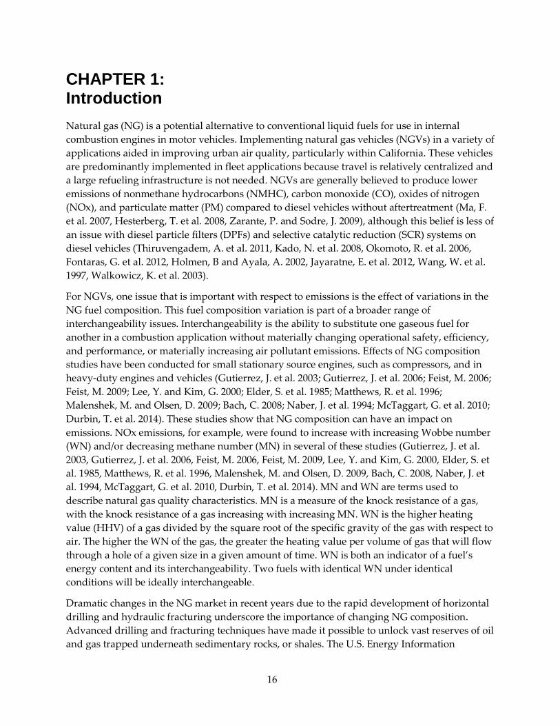
CHAPTER 1: Introduction

Natural gas (NG) is a potential alternative to conventional liquid fuels for use in internal

combustion engines in motor vehicles. Implementing natural gas vehicles (NGVs) in a variety of

applications aided in improving urban air quality, particularly within California. These vehicles

are predominantly implemented in fleet applications because travel is relatively centralized and

a large refueling infrastructure is not needed. NGVs are generally believed to produce lower

emissions of nonmethane hydrocarbons (NMHC), carbon monoxide (CO), oxides of nitrogen

(NOx), and particulate matter (PM) compared to diesel vehicles without aftertreatment (Ma, F.

et al. 2007, Hesterberg, T. et al. 2008, Zarante, P. and Sodre, J. 2009), although this belief is less of

an issue with diesel particle filters (DPFs) and selective catalytic reduction (SCR) systems on

diesel vehicles (Thiruvengadem, A. et al. 2011, Kado, N. et al. 2008, Okomoto, R. et al. 2006,

Fontaras, G. et al. 2012, Holmen, B and Ayala, A. 2002, Jayaratne, E. et al. 2012, Wang, W. et al.

1997, Walkowicz, K. et al. 2003).

For NGVs, one issue that is important with respect to emissions is the effect of variations in the

NG fuel composition. This fuel composition variation is part of a broader range of

interchangeability issues. Interchangeability is the ability to substitute one gaseous fuel for

another in a combustion application without materially changing operational safety, efficiency,

and performance, or materially increasing air pollutant emissions. Effects of NG composition

studies have been conducted for small stationary source engines, such as compressors, and in

heavy-duty engines and vehicles (Gutierrez, J. et al. 2003; Gutierrez, J. et al. 2006; Feist, M. 2006;

Feist, M. 2009; Lee, Y. and Kim, G. 2000; Elder, S. et al. 1985; Matthews, R. et al. 1996;

Malenshek, M. and Olsen, D. 2009; Bach, C. 2008; Naber, J. et al. 1994; McTaggart, G. et al. 2010;

Durbin, T. et al. 2014). These studies show that NG composition can have an impact on

emissions. NOx emissions, for example, were found to increase with increasing Wobbe number

(WN) and/or decreasing methane number (MN) in several of these studies (Gutierrez, J. et al.

2003, Gutierrez, J. et al. 2006, Feist, M. 2006, Feist, M. 2009, Lee, Y. and Kim, G. 2000, Elder, S. et

al. 1985, Matthews, R. et al. 1996, Malenshek, M. and Olsen, D. 2009, Bach, C. 2008, Naber, J. et

al. 1994, McTaggart, G. et al. 2010, Durbin, T. et al. 2014). MN and WN are terms used to

describe natural gas quality characteristics. MN is a measure of the knock resistance of a gas,

with the knock resistance of a gas increasing with increasing MN. WN is the higher heating

value (HHV) of a gas divided by the square root of the specific gravity of the gas with respect to

air. The higher the WN of the gas, the greater the heating value per volume of gas that will flow

through a hole of a given size in a given amount of time. WN is both an indicator of a fuel’s

energy content and its interchangeability. Two fuels with identical WN under identical

conditions will be ideally interchangeable.

Dramatic changes in the NG market in recent years due to the rapid development of horizontal

drilling and hydraulic fracturing underscore the importance of changing NG composition.

Advanced drilling and fracturing techniques have made it possible to unlock vast reserves of oil

and gas trapped underneath sedimentary rocks, or shales. The U.S. Energy Information

17

Administration (EIA) anticipates domestic NG production to continue to expand into the future,

growing from levels of 23.5 quadrillion British thermal units (Btu) in 2011 to a projected 33.9

quadrillion Btu in 2040, representing a sizable 44 percent increase (Energy Information

Administration 2013). Shale gas production, which already accounted for 23 percent of total

U.S. natural gas production in 2010, is expected to be the primary expansion driver, with shale

gas production going from 6.8 trillion cubic feet (tcf) in 2011 to 13.6 tcf in 2035 (Energy

Information Administration 2012). In California, the use of natural gas has also been increasing

for a number of years, primarily due to expanded power and home heating needs. Currently,

California supplies 85-90 percent of its needs with NG imported domestically from the Rockies,

from southwestern states, such as Texas, and from Canada. As new production fields are

developed in the United States, the makeup of imported domestic NG supplies could change.

Additionally, with the introduction of the Costa Azul LNG terminal in Baja California, Mexico,

there is the potential for NG from imported sources, such as the Pacific Rim, to become

available, especially for regions in the southern part of the state. LNG will also likely differ in

composition from what is currently used in California.

Natural gas quality depends on both its source as well as the degree to which it is processed.

Natural gas is produced from oil fields (termed associated gas) or from gas fields (termed

nonassociated gas). Associated gas is typically higher in heavier hydrocarbons, which gives the

gas a higher WN and a lower MN. Associated gas is often processed using techniques such as

refrigeration, lean oil absorption, and cryogenic extraction to recover valuable natural gas

liquids (NGLs) for other uses, such as ethane, propane, butanes, pentanes and hexanes plus

(NGC+ Interchangeability Work Group 2005, NGC+ Liquid Hydrocarbon Drop Out Task Group

2005). Traditional North American gas from Texas, for example, is often processed to recover

feedstock for chemical plants. This results in a natural gas stream with a lower WN and higher

MN. As the economics for these secondary products change, there could be a reduced emphasis

on recovering NGLs from NG. This could lead to NG with higher WNs and lower MNs being

fed into the pipeline, which would likewise result in a pipeline gas with a higher WN and lower

MN.

The present study’s objective is to evaluate the impact of NG composition on the performance

and exhaust emissions of heavy-duty vehicles. The California Air Resources Board (CARB) is

currently revisiting the compressed natural gas (CNG) fuel standards for motor vehicles (CARB

2015). Information on the impact of changing NG composition on performance and emissions

can be used for regulatory development, to ensure new NG compositions do not have an

adverse impact on air quality, and to evaluate the viability of using a broader mixture of NG

blends in transportation applications. For this study, four NG heavy-duty vehicles (HDVs) were

tested on a range of three to seven different test fuels. This included one NG school bus, one NG

waste hauler, and two NG class 8 trucks tested over the central business district cycle (CBD), the

Refuse Truck cycle, and segments of the drayage truck port cycle, respectively. The test fuels

included fuels representative of Texas Pipeline Gas and Rocky Mountain Pipeline Gas; a gas

representing Peruvian LNG modified to 1385 WN; a gas representing Middle East LNG-

Untreated (WN above 1400); two fuels with 1385 WNs and 75 MNs, one with a high ethane

content and the other with a high propane content; and one L-CNG fuel, which is a CNG blend

18

produced from an LNG fuel tank. In addition to the regulated emissions and fuel

economy/consumption, measurements were also made of ammonia (NH3), of carbonyls, of

nitrous oxide (N2O), and of particle number (PN) and particle size distributions. This report

discusses these test results. This study is part of the larger program that included the testing of

light-duty NGVs and other heavy-duty NGVs on a chassis dynamometer, which is discussed in

a previous report (Durbin, T. et al. 2014).

19

CHAPTER 2: Experimental Procedures

2.1 Test Fuels

The seven NG blends used for testing are characterized as follows:

Fuels H1 and H2 are representative of Texas and Rocky Mountain Pipeline gases. These

fuels are based on actual pipeline data. H1 serves as the baseline fuel.

Fuel LM3 is representative of Peruvian LNG that has been modified to meet a WN of

1385 and a MN of 75.

Fuel LM4 is representative of Middle East LNG-Untreated with a high WN (above 1400).

Fuel LM5 is a high ethane fuel with a WN of 1385 and a MN of 75.

Fuel LM6 is a high propane, high butane fuel with a WN of 1385 and a MN of 75.

Fuel H7 is representative of an L-CNG fuel sold in the South Coast Air Basin in 2014.

Test fuels H1 and H2 represent historical baseline gases for Southern California. Fuel H1,

“Baseline, Texas Pipeline,” refers to natural gas entering the Southern California Gas territory

through the El Paso Pipeline at Blythe and Topock and through the Transwestern Pipeline at

North Needles and Topock. Test gas H2 (Baseline, Rocky Mountain Pipeline) refers to natural

gas entering the Southern California Gas territory through the Kern/Mojave Pipeline at Wheeler

Ridge and Kramer Station. The actual test fuel compositions for H1 and H2 were derived by Air

Resources Board staff from fuel quality data submitted by the Southern California Gas

Company for the period from January 2000 to October 2010.

Fuels LM5 and LM6 are hypothetical fuels designed to see whether two fuels with the same WN

and MN, but different compositions, would produce different performance and exhaust

emissions. Natural gas with higher propane and butane is found locally in South Central Coast

region oil and gas fields, while natural gas with high ethane is found in San Joaquin Valley oil

and gas fields. Fuels LM5 and LM6 are both at the extremes for WN and MN, so the typical

local fuel in the pipeline in these areas will have lower WNs and higher MNs. This program

examines a wide range of scenarios to evaluate the viability of permitting the use of a broader

mixture of NG blends in transportation applications. Fuels LM3 to LM6 with lower methane

contents, and corresponding higher WNs and HHVs, and lower MNs are denoted as low

methane fuels throughout this report. Table 1 shows the test fuel specifications.

In addition, the CNG fueled John Deere school bus, waste hauler, and ISX12 G engines were run

on an L-CNG, identified as H7. Test fuel H7 is a historical fuel representing an L-CNG fuel sold

in the South Coast Air Basin in 2014. Test fuel H7 was included to capture the base line for these

engines that fuel on LNG. L-CNG is LNG that has been vaporized to a gas at the fueling station.

Although L-CNG was included as a test fuel to represent a waste hauler operating on LNG, a

LNG waste hauler would never see LM3, LM5, LM6 because these fuels have inert components.

20

LNG, on the other hand, has almost no inert components because inerts are removed during the

liquefaction process. LNG purchased at commercial fueling stations in the South Coast Air

Basin is manufactured from pipeline quality natural gas, which has been purified to remove

most of the hydrocarbon components heavier than methane as well as inert gases. The fuel is

refrigerated to minus 260 degrees for liquefaction, conversion to LNG. For this study, the

research team obtained L-CNG from a local fueling station for the school bus, the waste hauler,

and ISX12 G truck. The compositions for H7 for each of these vehicles are listed separately

based samples pulled from each vehicle.

Table 1: Test Fuel Specifications

Fuels # Description methane ethane propane I-butane N2 CO2 MN Wobbe # HHV H/C ratio

H1 Baseline,

Texas Pipeline 96 1.8 0.4 0.15 0.7 0.95 99 1338 1021 3.94

H2 Baseline,

Rocky Mountain Pipeline

94.5 3.5 0.6 0.3 0.35 0.75 95 1361 1046 3.89

LM3 Peruvian LNG 88.3 10.5 0 0 1.2 0 84 1385 1083 3.81

LM4 Middle East

LNG-Untreated 89.3 6.8 2.6 1.3 0 0 80 1428 1136 3.73

LM5 High Ethane 83.65 10.75 2.7 0.2 2.7 0 75.3 1385 1115 3.71

LM6 High Propane 87.2 4.5 4.4 1.2 2.7 0 75.1 1385 1116 3.70

H7 L-CNG fuel (waste hauler)

98.42 1.26 0.05 0.02 0.25 0 104.5 1339 1004 3.97

H7 L-CNG fuel (school bus)

95.24 4.39 0.11 0.01 0.25 0 97 1352 1029 3.91

H7 L-CNG fuel (ISX12 G truck)

94.63 4.61 0.14 0.02 0.55 0 96 1347 1027 3.91

MN = Methane Number determined via CARB calculations; Wobbe # = HHV/square root of the specific gravity of the blend with respect to air; HHV = Higher Heating Value; H/C = ratio of hydrogen to carbon atoms in the hydrocarbon portion of the blend

* Properties evaluated at 60 °F (15.6 °C) and 14.73 psi (101.6 kPa)

Source: CE-CERT

2.1.1 Fuel Composition and Rich and Lean Combustion

Older lean burn engines have been observed to operate at slightly richer air-fuel (A/F) ratios

during combustion when running on low methane fuels (Feist, M. 2006, 2009). Rich operation or

rich combustion, as used throughout this report, means that the combustion is taking place at

an A/F ratio that is lower than that for stoichiometric combustion. The A/F ratio for

21

stoichiometric combustion represents the ratio where there is exactly enough air to completely

burn all of the fuel during combustion. For rich combustion, the A/F ratio is lower than that for

stoichiometric combustion, meaning that the amount of air is not fully sufficient to burn all of

the fuel during combustion. Regardless of whether the actual combustion is rich, lean, or

stoichiometric, as the A/F ratio for combustion decreases between any two points in time, the

combustion is richer than the initial condition.

2.2 Test Vehicles

Four vehicles were selected to represent different vehicle types: a school bus, waste hauler, and

two class 8 trucks, and different types of engines. The inclusion of the three vehicle types

provides some information on the differences between school bus, waste hauler, and port-

related service vehicles.

The school bus used a 2005 lean-burn combustion John Deere 8.1 L 6081H engine, with an

oxidation catalyst (OC). The waste hauler was fitted with a 2011 8.9L stoichiometric spark

ignited Cummins Westport ISL-G engine with cooled exhaust gas recirculation (EGR) and a

three-way catalyst (TWC). This vehicle was selected to represent the latest engine technology

available for natural gas engines. The third vehicle was equipped with a 2012 Cummins

Westport ISL G 8.9 L stoichiometric engine, with a three-way catalyst (TWC) and a cooled

exhaust gas recirculation (EGR) system. The fourth vehicle was a 2013 Cummins Westport

ISX12 G stoichiometric engine, with a TWC device and a cooled EGR system. Table 2 provides

the engine specifications. The certification Executive Orders for each of the engines tested are

provided in Appendix A. The Colton Unified School District provided the school bus on loan.

Waste Management provided the waste hauler. The Cummins trucks were leased from Ryder

Truck Leasing, local to Riverside, California.

22

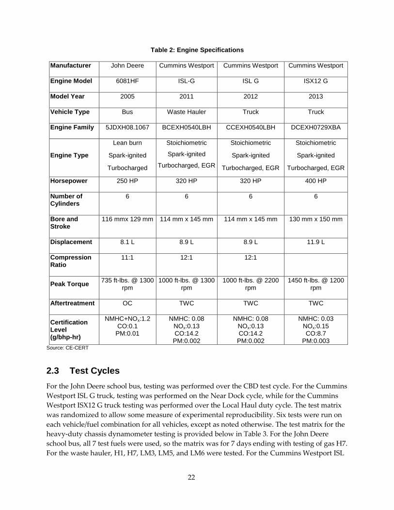
Table 2: Engine Specifications

Manufacturer John Deere Cummins Westport Cummins Westport Cummins Westport

Engine Model 6081HF ISL-G ISL G ISX12 G

Model Year 2005 2011 2012 2013

Vehicle Type Bus Waste Hauler Truck Truck

Engine Family 5JDXH08.1067 BCEXH0540LBH CCEXH0540LBH DCEXH0729XBA

Engine Type

Lean burn

Spark-ignited

Turbocharged

Stoichiometric

Spark-ignited

Turbocharged, EGR

Stoichiometric

Spark-ignited

Turbocharged, EGR

Stoichiometric

Spark-ignited

Turbocharged, EGR

Horsepower 250 HP 320 HP 320 HP 400 HP

Number of Cylinders

6 6 6 6

Bore and Stroke

116 mmx 129 mm 114 mm x 145 mm 114 mm x 145 mm 130 mm x 150 mm

Displacement 8.1 L 8.9 L 8.9 L 11.9 L

Compression Ratio

11:1 12:1 12:1

Peak Torque 735 ft-lbs. @ 1300

rpm 1000 ft-lbs. @ 1300

rpm 1000 ft-lbs. @ 2200

rpm 1450 ft-lbs. @ 1200

rpm

Aftertreatment OC TWC TWC TWC

Certification Level (g/bhp-hr)

NMHC+NOx:1.2 CO:0.1

PM:0.01

NMHC: 0.08 NOx:0.13 CO:14.2 PM:0.002

NMHC: 0.08 NOx:0.13 CO:14.2 PM:0.002

NMHC: 0.03 NOx:0.15 CO:8.7

PM:0.003 Source: CE-CERT

2.3 Test Cycles

For the John Deere school bus, testing was performed over the CBD test cycle. For the Cummins

Westport ISL G truck, testing was performed on the Near Dock cycle, while for the Cummins

Westport ISX12 G truck testing was performed over the Local Haul duty cycle. The test matrix

was randomized to allow some measure of experimental reproducibility. Six tests were run on

each vehicle/fuel combination for all vehicles, except as noted otherwise. The test matrix for the

heavy-duty chassis dynamometer testing is provided below in Table 3. For the John Deere

school bus, all 7 test fuels were used, so the matrix was for 7 days ending with testing of gas H7.

For the waste hauler, H1, H7, LM3, LM5, and LM6 were tested. For the Cummins Westport ISL

23

G truck, only H1, LM5, and LM6 were tested. For the Cummins Westport ISX12 G truck, H1,

LM4, LM5, and H7 were tested.

Table 3: Chassis Dynamometer Test Matrix for Each Test Vehicle

Test Day

Morning Schedule Afternoon Schedule

(assumes 3 replicates)

(assumes 3 replicates)

ISL G – Near Dock

Day 1 H1,H1,H1 LM5,LM5,LM5

Day 2 LM5,LM5,LM5 LM6,LM6,LM6

Day 3 LM6,LM6,LM6 H1,H1,H1

ISL G – Waste Hauler

Day 1 H7,H7,H7 H1,H1,H1





John Deere - CBD

Day 1 H7,H7,H7 H1,H1,H1

Day 2 H1,H1,H1 H2,H2,H2






ISX12 G – Local Hauler

Day 1 H7,H7,H7 H1,H1,H1




CBD = Central Business District; WHM = William H. Martin;

Source: CE-CERT

A specially developed cycle was used for the CBD testing. This cycle consisted of a single CBD

cycle as a warm-up, followed by a double (i.e., two iterations) CBD cycle. The CBD cycle was

repeated twice to provide a sufficient particle sample for analysis. The CBD cycle is

characterized by an average speed of 20.23 kilometers per hour (km/h), a maximum speed of

32.18 km/h [20 miles per hour (mph)], an average acceleration of 0.89 meters per second squared

24

(m/s2), a maximum acceleration of 1.79 m/s2. The driving distance for a single CBD cycle is 3.22

km, or 9.66 km for the full cycle, including the warm-up. Emission analyses for gaseous

emissions were collected as an integrated sample over the double CBD cycle. West Virginia

University (WVU) used a similar cycle in earlier testing on CNG buses (Walkowicz, K. et al.

2003). A speed-time trace for the extended CBD is provided in Figure 1.

Figure 1: Double CBD Cycle with Warm-up

0

5

10

15

20

25

0 200 400 600 800 1000 1200 1400 1600 1800

Sp

eed

(m

ph

)

Time

Source: CE-CERT

The waste hauler was tested over the William H. Martin (WHM) Refuse Truck Cycle. WVU

developed this cycle to simulate waste hauler operation. The cycle consists of a transport

segment, a curbside pickup segment, and a compaction segment. The initial 277-second

segment of the cycle is a warm-up period where no emissions were collected. The transport

portion of the cycle represents the first 300 seconds of the actual cycle for the trip out to the

service area and the 300 seconds after the curbside segment for the return trip from the service

area. The first and second part of the transport cycle represents different types of driving

conditions that a waste hauler might do. The curbside pickup portion of the cycle is 520

seconds. It is the middle portion of the cycle with a series of low speed accelerations. The

compaction portion of the cycle is the final phase. Before the start of the actual compaction cycle

where emission data is collected, there is an interval for an acceleration up to and stabilization

at the appropriate test speed. Data collection for the compaction phase begins once the vehicle

has stabilized at the test speed for the compaction, and data for the compaction phase is

collected for a period of 155 seconds. The compaction load is simulated by applying a

predetermined torque to the drive axle while maintaining a fixed speed of 45 mph. The

compaction load used in this study was 80 horsepower (hp), the same as used previously by

WVU (Walkowicz, K. et al. 2003). The Refuse Truck Cycle is shown in Figure 2.

Start of Data Collection: 560s

End of Test: 1680s

25

Figure 2: Refuse Truck Cycle

0

10

20

30

40

50

60

0 200 400 600 800 1000 1200 1400 1600 1800

Spee

d (

mp

h)

Time (sec)

Source: CE-CERT

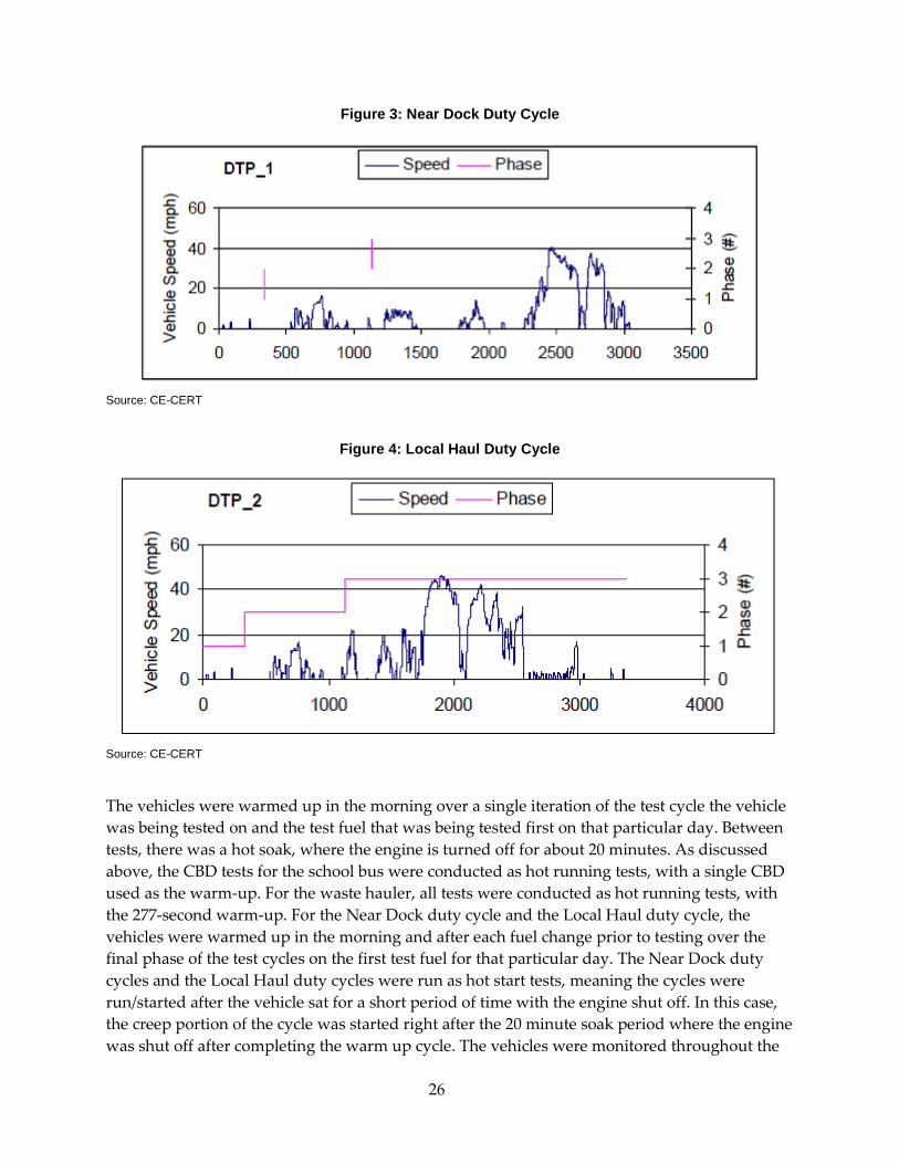
The Near Dock duty cycle and the Local Haul duty cycle are segments of the drayage truck port

cycle developed by TIAX in conjunction with the Ports of Long Beach and Los Angeles. These

cycles were developed based on data logging of over 1,000 Class 8 drayage trucks at these ports

for trips over a four-week period in 2010. The Near Dock duty cycle consists of three different

phases: a creep phase, a low speed transient phase, and a short high-speed transient phase. The

cycle covers a total distance of 5.61 miles with an average speed of 6.6 mph and a maximum

speed of 40.6 mph. Similar to the Near Dock duty cycle, the Local Haul duty cycle also consists

of three different phases, with the creep phase and the low speed transient phase being the

same as the Near Dock cycle. The Local Haul duty cycle; however, consists of a long high-speed

transient phase. The cycle covers a total distance of 8.71 miles with an average speed of 9.3 mph

and a maximum speed of 46.4 mph. The Near Dock Cycle and the Local Haul duty cycle are

shown in Figure 3 and Figure 4.

Start of

Data

Collection

Warm up

for 277s

Transport

1st Segment

Curbside

Transport

2nd

Segment Compaction

Data

Collection

for 155s

No Data

Collection

26

Figure 3: Near Dock Duty Cycle

Source: CE-CERT

Figure 4: Local Haul Duty Cycle

Source: CE-CERT

The vehicles were warmed up in the morning over a single iteration of the test cycle the vehicle

was being tested on and the test fuel that was being tested first on that particular day. Between

tests, there was a hot soak, where the engine is turned off for about 20 minutes. As discussed

above, the CBD tests for the school bus were conducted as hot running tests, with a single CBD

used as the warm-up. For the waste hauler, all tests were conducted as hot running tests, with

the 277-second warm-up. For the Near Dock duty cycle and the Local Haul duty cycle, the

vehicles were warmed up in the morning and after each fuel change prior to testing over the

final phase of the test cycles on the first test fuel for that particular day. The Near Dock duty

cycles and the Local Haul duty cycles were run as hot start tests, meaning the cycles were

run/started after the vehicle sat for a short period of time with the engine shut off. In this case,

the creep portion of the cycle was started right after the 20 minute soak period where the engine

was shut off after completing the warm up cycle. The vehicles were monitored throughout the

27

course of testing for differences in the operability of the engine on the different blends, such as

knock. No significant differences in operability of the engine on the different test blends were

observed during the course of normal testing.

The road load coefficients were calculated based on the frontal area of the vehicle and a factor

accounting for its general shape for the school bus and the two class 8 trucks. The road load

coefficients for the waste hauler were the same as that used in the first round testing of the

waste hauler testing, determined by coasting down the vehicle from approximately 60 mph to

approximately 10 mph (Durbin, T. et al. 2014). The test weight used for the school bus was

30,560 lbs. based on procedures similar to those used in a recent study (Durbin, T. et al. 2014).

The test vehicle for the waste hauler was the same as that used in the first round testing of the

waste hauler testing (i.e., 33,520 lbs.). The test weight used for the two class 8 trucks was 56,000

lbs., which is a typical weight for trucks hauling goods in the local port areas.

2.4 Emissions Testing and Measurements

The chassis dynamometer testing was conducted in University of California, Riverside (UCR)

Center for Environmental Research and Technology’s (CE-CERT’s) heavy-duty chassis

dynamometer facility. UCR’s chassis dynamometer is an electric AC type design that can

simulate inertia loads from 10,000 lb. to 80,000 lb. This covers a broad range of in-use medium

and heavy-duty vehicles. The design incorporates 48” rolls, axial loading to prevent tire

slippage, 45,000 lb base inertial plus two large AC drives for achieving a range of inertias. The

dynamometer has the capability to absorb accelerations and decelerations up to 6 mph/sec and

handle wheel loads up to 600-horse power at 70 mph. This facility was also specially geared to

handle slow speed vehicles such as yard trucks where 200 hp at 15 mph is common.

The chassis dynamometer was designed to accurately perform the new CARB 4-mode cycle, the

urban dynamometer driving schedule (UDDS), refuse drive schedules (WHM), bus cycles (like

the central business district [CBD] cycle), as well as a range of other speed vs time traces. The

load measurement uses state of the art sensing and is accurate to 0.05 percent of full scale and

has a response time of less than 100 ms, which is necessary for repeatable and accurate transient

testing. The speed accuracy of the rolls is ± 0.01 mph and has acceleration accuracy of ± 0.02

mph/sec, both measured digitally and thus easy to maintain their accuracy. The torque

transducer is calibrated as per Code of Federal Regulations (CFR) 1065, which is a standard

method used for determining accurate and reliable wheel loads. A typical vehicle set up on the

chassis dynamometer is shown in Figure 5.

28

Figure 5: Typical Setup of Test Vehicles on the Chassis Dynamometer

Photo Credit: CE-CERT

The CE-CERT team obtained the emission measurements using its Mobile Emissions Laboratory

(MEL). For all tests, standard emissions measurements of total hydrocarbons (THC), NMHC,

methane (CH4), CO, NOx, carbon dioxide (CO2), and PM, were measured. The 602P

nondispersive infrared (NDIR) analyzer from California Analytical Instruments (CAI)

measured the CO and CO2 emissions. THC, NMHC, and CH4 emissions were measured with

600HFID flame ionization detector (FID) from CAI. NOx emissions were measured with

600HPLC chemiluminescence analyzer from CAI. Measurements were also made of NH3 using

a tunable diode laser (TDL) from Unisearch Associates Inc. LasIR S Series that is incorporated in

the MEL. Measurements of nitrous oxide (N2O) were made using a Fourier Transform Infrared

(FTIR).

The mass concentrations of PM2.5 were obtained by analysis of particulates collected on 47mm

diameter 2μm pore Teflo filters (Whatman brand). The filters were measured for net gains using

a UMX2 ultra precision microbalance with buoyancy correction following the CFR weighing

procedure guidelines.

The sampling of carbonyls was done for 3-4 tests per test fuel/vehicle combination. Samples for

carbonyl analysis were collected onto 2, 4-dinitrophenylhydrazine (DNPH) coated silica

cartridges (Waters Corp., Milford, MA). A critical flow orifice controls the flow to 1.0 liter per

29

minute through the cartridge. Sampled cartridges were extracted using 5 mL of acetonitrile and

injected into an Agilent 1200 series high performance liquid chromatograph (HPLC) equipped

with a variable wavelength detector. The column used was a 5 μm Deltabond AK resolution

(200cm x 4.6mm ID) with upstream guard column. The HPLC sample injection and operating

conditions were set up according to the specifications of the SAE 930142HP protocol (Siegl, W.

et al. 1993). Samples from the dilution air were collected for background correction.

Sampling for carbonyl compounds and the PM mass was done cumulatively over the entire

duration of each test cycle due to the low mass levels expected for these pollutants and the

corresponding need to collect a sufficient sample for analysis. As such, results for the individual

modes of the Refuse Truck cycle, Near Dock duty cycle, and the Local Hauler duty cycle are not

available for these pollutants. The FTIR N2O measurements were also made from bag samples

that collected cumulatively over the duration of each cycle. A schematic of the experimental

setup is provided in Figure 6.

Particle number counts were measured with a TSI 3776 ultrafine-Condensation Particle Counter

(CPC) with a 2.5 nm cut point. An Engine Exhaust Particle Sizer (EEPS) spectrometer (TSI 3090,

firmware version 8.0.0) measured real-time second-by-second particle size distributions

between 5.6 to 560 nm. The EEPS has a scan time of one second and provides a size range from

6 to 423 nm in electrical mobility. Particles were sampled at a flow rate of 10 L/min for the EEPS,

which is considered high enough to minimize diffusional losses. A corona charger then charged

the particles and determined the size based on their electrical mobility in an electrical field.

Concentrations were determined using multiple electrometers.

30

Figure 6: Schematic of the Sampling Systems and Instruments

CVS Sampling System – Primary Dilution Tunnel

Vehicle Exhaust Particle size distribution - Regular-column

SMPS/nano-SMPS/EEPS

Carbonyls - DNPH cartridges

NOx- Chemiluminescence

CO-NDIR

CO2-NDIR

THC-heated FID

CH4-FID

Gas sample probe

Secondary

Dilution

Tunnel

PN-TSI 3776 CPC

PM mass

Raw Exhaust

NH3-TDL

Source: CE-CERT

31

CHAPTER 3: Heavy-Duty Vehicle Chassis Dynamometer Testing Results

The emissions results are presented in the following section. The figures for each pollutant

show the results for each vehicle/fuel/cycle combination based on the average of tests conducted

on that particular test combination. The error bars on the figures are the standard deviation over

all tests for each test combination. The average emissions test results with percentage

differences between fuels and p-values for statistical analyses are provided in Appendix B. The

statistical analyses were conducted using a 2-tailed, 2 sample equal variance t-test. For the

statistical analyses, results are considered to be statistically significant for p ≤ 0.05, or marginally

statistically significant for 0.05 < p ≤ 0.1 in this analysis. To provide a better representation of the

results, the emission pollutants for the class 8 trucks over the Near Dock and Local Haul duty

cycles are shown for each of the individual phases of the cycle, i.e., the creep phase, the low

speed transient phase, and the short high-speed transient phase.

3.1 Nitrogen Oxides Emissions

Figure 7 shows the NOx emissions for the John Deere school bus. Fuel composition influences

NOx emission levels for the school bus, with the low methane fuels resulting in higher NOx

emissions compared to the high methane fuels. The school bus showed statistically significant

increases of 33.5 percent, 35.1 percent, 25.6 percent, and 14.2 percent, respectively for LM3, LM4,

LM5, and LM6 compared to H1. Statistically significant increases in NOx emissions were also

seen for H2 (11.4 percent) and H7 (6.6 percent) relative to H1. Compared to H2, NOx emissions

showed statistically significant increases of 19.8 percent, 21.2 percent, and 12.7 percent,

respectively, for LM3, LM4, and LM5, whereas H1 showed a statistically significant reduction in

NOx emissions of 10.2 percent. Similar to H1 and H2 fuels, NOx emissions showed statistically

significant increases of 25.1 percent, 26.7 percent, 17.7 percent, and 7.1 percent, respectively, for

LM3, LM4, LM5, and LM6 compared to H7, whereas H1 showed a NOx reduction of 6.2 percent

at a statistically significant level.

32

Figure 7: Average NOx Emissions for the John Deere Bus

H1: Texas (1339 WN), H2: Rocky Mtn (1361 WN), LM3: Peruvian LNG (1385 WN), LM4: Middle East LNG (1428 WN), LM5: Hi Ethane (1385 WN), LM6: Hi Propane (1385 WN), H7: L-CNG (1370 WN)

Source: CE-CERT

The increases in NOx emissions with LM3, LM4, LM5, and LM6 fuels for the lean-burn engine

fitted with the oxidation catalyst can be attributed to the presence of high molecular-weight

hydrocarbons in these fuels. The addition of higher hydrocarbons (ethane and propane) can

increase the adiabatic flame speed. As flame speed increases at constant ignition timing, peak

pressure occurs earlier, at smaller cylinder volumes, and higher temperatures result. Peak

combustion temperatures are higher due to the advanced location of peak pressure and higher

adiabatic flame temperature (Fiest, M. et al. 2010), which would result in higher NOx emissions,

as NOx is generated predominantly through the strongly temperature-dependent thermal NO

mechanism (McTaggart, G. et al. 2010, Naber, J. et al. 1994). Previous studies have also shown

that lean-burn engines run richer as MN is decreased (Fiest, 2009). This reaction can lead to the

oxidation of more fuel, higher combustion temperatures, and increased cylinder pressures. It is

also possible that the higher hydrocarbons promote the formation of reactive radicals, which

33

result in increased formation of prompt NOx. The results reported here are also in agreement

with previous studies conducted at UCR CE-CERT utilizing lean-burn engines on low methane

fuels (Karavalakis, G. et al. 2013; Hajbabaei, M. et al. 2013), where higher NOx emissions are

seen with low methane fuels are seen for transit buses and a waste hauler equipped with lean-

burn engines and operated over the CBD cycle and the Refuse Truck cycle (RTC), respectively.

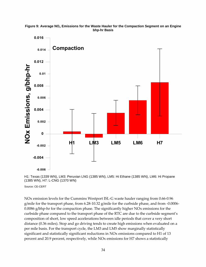
Error! Reference source not found. (a-b) shows the emissions of NOx in grams (g) per mile for

the waste hauler for the transport and curbside segments of the Refuse Truck Cycle. Error!

Reference source not found. shows the emissions of NOx for the waste hauler for the

compaction segment of the Refuse Truck Cycle. For the compaction segment, the emissions are

presented on a brake horsepower-hour (bhp-hr) basis based on readings from the engine’s

control module (ECM). Bhp-hr is an important emission measurement metric, since the

compaction segment is not designed to represent a driving cycle and since heavy-duty natural

gas engines are certified on a bhp-hr basis.

Figure 8 (a-b): Average NOx Emissions for the Waste Hauler Transport and Curbside Segments

H1: Texas (1339 WN), LM3: Peruvian LNG (1385 WN), LM5: Hi Ethane (1385 WN), LM6: Hi Propane (1385 WN), H7: L-CNG (1370 WN)

Source: CE-CERT

34

Figure 9: Average NOx Emissions for the Waste Hauler for the Compaction Segment on an Engine bhp-hr Basis


Source: CE-CERT

NOx emission levels for the Cummins Westport ISL-G waste hauler ranging from 0.66-0.96

g/mile for the transport phase, from 6.28-10.32 g/mile for the curbside phase, and from -0.0006-

0.0086 g/bhp-hr for the compaction phase. The significantly higher NOx emissions for the

curbside phase compared to the transport phase of the RTC are due to the curbside segment’s

composition of short, low speed accelerations between idle periods that cover a very short

distance (0.36 miles). Stop and go driving tends to create high emissions when evaluated on a

per mile basis. For the transport cycle, the LM3 and LM5 show marginally statistically

significant and statistically significant reductions in NOx emissions compared to H1 of 13

percent and 20.9 percent, respectively, while NOx emissions for H7 shows a statistically

35

significant increase of 15.1 percent compared to H1. For the curbside cycle, LM3 and LM6

demonstrated a 24.3 percent and 17.4 percent reduction in NOx emissions compared to H1,

respectively, while NOx emissions for H7 shows a statistically significant increase of 24.2

percent compared to H1. NOx emissions for the compaction cycle are at very low levels and

considerably below the 0.2 g/bhp-hr standard. Statistically significant increases in NOx

emissions are seen for LM6 and H7 compared to H1 on the order of 1,323 percent and 2,086

percent, respectively, while LM5 shows a marginally statistically significant increase in NOx

emissions of 779 percent compared to H1. The high percentage increases for the compaction

cycle can be attributed to the very low emission levels, and that these differences are relatively

small on an absolute basis.

The results reported here show substantially lower NOx emission levels than those found in the

Phase 1 part of this study (Durbin, T. e al. 2014) for a legacy waste hauler equipped with a 2002

Cummins 8.3L C Gas Plus, lean burn, spark ignited engine using the same gas blends and

operated over the RTC. Several studies have shown that the majority of NOx reductions can be

attributed to the TWC (Einewall, P. et al. 2005, Chiu, J. 2007). The newer stoichiometric engine

tested in this study also has EGR that introduces inert exhaust gases into the combustion

cylinder, which reduces cylinder combustion temperature and results in lower NOx emissions.

The slight decrease in NOx emissions for the low methane fuels may be due to slightly richer

air/fuel (A/F) ratios for combustion. The resultant decrease in oxygen may also lead to increased

effectiveness in the TWC’s ability to further reduce NOx emissions. Previously, lean burn

engines have also been observed to operate with a slightly richer A/F ratio when running on

low methane fuels (Feist, M. 2006). In this case, the engines experienced increased NOx

emissions, which had been attributed to higher flame speeds and adiabatic flame temperatures

(Feist, M. 2006, Durbin, T. 2014). Stoichiometric engines generally exhibit tighter A/F ratio

control, so any change in the A/F ratio should be slight with minimal engine effects; however,

along with decreases in NOx emissions from operation on low methane fuels, the refuse hauler

exhibited increased CO emissions as discussed in Section 3.5, which is consistent with slightly

richer combustion.

Figure 10 shows the NOx emissions for the Cummins Westport ISL G (A) and Cummins

Westport ISX12 G (B) Class 8 trucks. NOx emissions for both trucks are presented for the three

individual phases of the Near Dock cycle and the Local Haul Duty cycle as well as for the

accumulated cycle. The Cummins ISX12 G truck produces substantially lower NOx emission

levels than the Cummins ISL G truck. Both vehicles showed the highest emissions for the creep

phase of the test cycle. Both Cummins trucks and the low MN/high Wobbe number fuels

generally show lower NOx levels than the high methane fuels. This reduction in NOx levels is

opposite to the trends for the lean-burn John Deere engine, where the low methane fuels clearly

produce higher NOx emissions than the baseline fuels.

For the Cummins ISL G truck, the accumulated NOx emissions show some trends towards

lower emissions with the low methane fuels, i.e., LM5 and LM6, compared to H1. NOx

emissions show statistically significantly reductions of 36.7 percent for LM6 compared to H1.

Emissions of NOx are considerably higher for the creep phase than the other two phases of the

36

Near Dock duty cycle. For the creep phase, there are no strong fuel effects in NOx emissions.

For the low speed transient phase, NOx emissions show a marginally statistically significant

decrease of 21.5 percent and a statistically significant decrease of 26.5 percent, respectively, for

LM5 and LM6 compared to H1. For the short high-speed transient phase, NOx levels show a

statistically significant decrease of 50.2 percent for LM6 compared to H1.

For the Cummins Westport ISX12 G truck, the accumulated NOx emissions generally show

weak trends between fuels with the exception of LM5, which shows marginally statistically

significant reductions of 19.3 percent and 20.2 percent, respectively, compared to H1 and H2.

While some trends towards lower NOx emissions are observed for the low methane fuels for

each individual phase of the Local Haul duty cycle, there are no statistically significant

differences between fuels.

Figure 10: NOx Emissions for the Class 8 Trucks Cummins Westport ISL G Over the Near Dock Cycle (A) and Cummins Westport ISX12 G Over the Local Haul Duty Cycle (B) for Their Individual

Phases

37

H1: Texas (1339 WN), LM4: Middle East LNG (1428 WN), LM5: Hi Ethane (1385 WN), LM6: Hi Propane (1385 WN), L-CNG: (1370 WN); Phase 1 = creep phase and Phase 2 = a low speed transient phase for both trucks. For the ISL-G Phase 3 is a short high-speed transient phase and for the ISX12G Phase 3 is a long high-speed transient phase.

Source: CE-CERT

3.2 Total Hydrocarbon Emissions

Figure 11 shows the THC emissions for the John Deere school bus over the CBD cycle. THC

emissions show a trend of reductions for the low methane fuels compared to the high methane

fuels. THC emissions are lower at a statistically significant level by 9.8 percent, 17.4 percent,

13.4 percent, 11.6 percent, and 8.2 percent, respectively, for LM3, LM4, LM5, LM6, and H7

compared to H1. Compared to H2, THC emissions also show statistically significant decreases

of 9 percent, 16.7 percent, 12.6 percent, 10.8 percent, and 7.4 percent, respectively, for LM3,

LM4, LM5, LM6, and H7. Compared to H7, THC emissions show statistically significant

increases of 8.9 percent and 7.9 percent, respectively, for H1 and H2, while LM4 shows a

statistically significant decrease of 10.1 percent.

38

Figure 11: Average THC Emissions for the John Deere Bus


Source: CE-CERT

Figure 12 (a-b) shows the THC emissions for the waste hauler for the transport and curbside

segments, while Figure 13 shows the THC emissions for the compaction segment on a bhp-hr

basis. THC emissions are significantly lower than typically found for older lean burn NG

engines equipped with oxidation catalysts (OCs). This reduction in THC emissions can be

attributed to the differences in engine technology, since older engines are lean-burn engines

with OCs designed to meet an earlier certification standard, and the ISL-G is a stoichiometric

engine with a TWC that is designed to meet a more recent and stringent certification standard

(The International Council on Clean Transportation, 2009). Overall, THC emissions do not show

strong fuel trends. There are no statistically significant differences between fuels for the

transport and curbside phases of the RTC. The only statistically significant differences are for

39

LM3 and LM5 compared to H7, which shows a statistically significant 29 percent increase in

THC emissions and a marginally statistically significant increase of 26 percent, respectively. For

the compaction cycle, LM3 is higher (22.2 percent) than H1 at a statistically significant level,

while LM6 is higher (16.4 percent) than H1 at a marginally statistically significant level.

Although the low methane fuels over the compaction cycle showed some trends toward higher

THC emissions, there are no consistent fuel trends over the different RTC phases. The results

show that the differences in the hydrocarbon composition of the test fuels do not influence the

THC emission control systems effectiveness.

Figure 12 (a-b): Average THC Emissions for Waste Hauler Transport and Curbside Segments


Source: CE-CERT

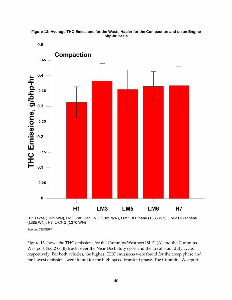
40

Figure 13: Average THC Emissions for the Waste Hauler for the Compaction and on an Engine bhp-hr Basis


Source: CE-CERT

Figure 13 shows the THC emissions for the Cummins Westport ISL G (A) and the Cummins

Westport ISX12 G (B) trucks over the Near Dock duty cycle and the Local Haul duty cycle,

respectively. For both vehicles, the highest THC emissions were found for the creep phase and

the lowest emissions were found for the high-speed transient phase. The Cummins Westport

41

ISL G truck showed higher THC emissions for the creep phase, but not for the low speed

transient phase.

For the Cummins Westport ISL G truck, the accumulated THC emissions show statistically

significant reductions of 20.5 percent and 15.7 percent, respectively, for LM5 and LM6

compared to H1. For the individual phases of the Near Dock cycle, THC emissions show a

declining trend with the low methane fuels relative to H1. For the creep phase, THC emissions

show a statistically significant decrease of 32.5 percent for LM5 compared to H1, while for the

low speed transient phase both the LM5 and LM6 showed decreases of 31.4 percent and 31.2

percent, respectively, compared to H1 at a statistically significant level.

For the Cummins Westport ISX12 G truck, accumulated THC emissions do not show large

differences between the test fuels, although some trends towards lower THC emissions for the

low methane fuels are observed. A marginally statistically significant decrease in the

accumulated THC emissions is also seen for LM5 (16 percent) compared to H7. For the low

speed transient phase, THC emissions show statistically significant decreases of 17.2 percent for

LM4 compared to H1, and 26 percent and 22.3 percent, respectively, for LM4 and LM5

compared to H7. For the long high-speed transient phase, THC emissions show statistically

significant decreases of 32.4 percent and 18 percent, respectively, for LM5 compared to H1 and

H7.

42

Figure 14: THC Emissions for the Class 8 Trucks Cummins Westport ISL G Over the Near Dock Cycle (A) and Cummins Westport ISX12 G Over the Local Haul Duty Cycle (B) for Their Individual

Phases

H1: Texas (1339 WN), H2: Rocky Mtn (1361 WN), LM3: Peruvian LNG (1385 WN), LM4: Middle East LNG (1428 WN), LM5: Hi Ethane (1385 WN), LM6: Hi Propane (1385 WN), H7: L-CNG (1370 WN); Phase 1 = creep phase and Phase 2 = a low speed transient phase for both trucks. For the ISL-G Phase 3 is a short high-speed transient phase and for the ISX12G Phase 3 is a long high-speed transient phase.

Source: CE-CERT

THC emissions are significantly lower for the stoichiometric Cummins Westport engines

compared to the John Deere lean-burn engine. This reduction in THC emissions can be

attributed to the differences in the engine technology, since the older technology lean-burn John

Deere engine is fitted with an OC designed to meet an earlier certification standard, while the

stoichiometric Cummins engines are fitted with TWC devices designed to meet a more recent,

more stringent certification standard (Einewall, P. et al. 2005, The International Council on

43

Clean Transportation 2009). The John Deere school bus and the Cummins trucks show trends of

higher THC emissions for the high methane fuels. This trend is consistent with results

previously reported by other authors (Wang, W. et al. 1997), and also in agreement with

previous studies conducted at CE-CERT (Karavalakis, G. et al. 2013, Hajbabaei et al. 2013). This

result is probably due to the THC emissions from these engine/aftertreatment types, which are

predominantly methane. The discussion below describes the trend, as the CH4 emissions are

roughly comparable to the THC emissions, while the NMHC emissions are very low. The

reduction in THC emissions for the low methane fuels could also be due to more complete

oxidation of the fuel as the combustion temperatures increase, as discussed under the NOx

section. CH4 is also less reactive from a combustion standpoint than higher hydrocarbons

(Burcat, A. et al. 1971), so it is more likely to go through the combustion process unburned and

pass unreacted across the catalyst.

3.3 Nonmethane Hydrocarbon Emissions

Figure 15 shows the NMHC emissions for the John Deere school bus over the CBD test cycle.

Emissions of NMHC show strong fuel trends for the John Deere bus, with the low methane

fuels producing higher NMHC emissions than the high methane fuels. The NMHC emissions

show statistically significant increases of 26.3 percent, 94.1 percent, 91.3 percent, 133.2 percent,

and 106.1 percent, respectively, for H2, LM3, LM4, LM5, and LM6 compared to H1. Compared

to H2, all test fuels show statistically significant differences in NMHC emissions with the low

methane fuels showing statistically significant increases and the high methane fuels showing

statistically significant decreases. Similar to H2, all test fuels showed statistically significant

increases in NMHC emissions compared to H7 ranging from 21.9 percent to 125.1 percent, with

the exception of H1.

44

Figure 15: Average NMHC Emissions for the John Deere Bus


Source: CE-CERT

Figure 16 (a-b) shows the NMHC emissions for the waste hauler for the transport and curbside

segments, while Figure 17

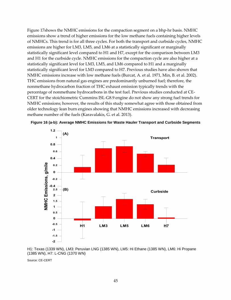
45

Figure 17shows the NMHC emissions for the compaction segment on a bhp-hr basis. NMHC

emissions show a trend of higher emissions for the low methane fuels containing higher levels

of NMHCs. This trend is for all three cycles. For both the transport and curbside cycles, NMHC

emissions are higher for LM3, LM5, and LM6 at a statistically significant or marginally

statistically significant level compared to H1 and H7, except for the comparison between LM3

and H1 for the curbside cycle. NMHC emissions for the compaction cycle are also higher at a

statistically significant level for LM3, LM5, and LM6 compared to H1 and a marginally

statistically significant level for LM3 compared to H7. Previous studies have also shown that

NMHC emissions increase with low methane fuels (Burcat, A. et al. 1971, Min, B. et al. 2002).

THC emissions from natural gas engines are predominantly unburned fuel; therefore, the

nonmethane hydrocarbon fraction of THC exhaust emission typically trends with the

percentage of nonmethane hydrocarbons in the test fuel. Previous studies conducted at CE-

CERT for the stoichiometric Cummins ISL-G8.9 engine do not show any strong fuel trends for

NMHC emissions; however, the results of this study somewhat agree with those obtained from

older technology lean burn engines showing that NMHC emissions increased with decreasing

methane number of the fuels (Karavalakis, G. et al. 2013).

Figure 16 (a-b): Average NMHC Emissions for Waste Hauler Transport and Curbside Segments


Source: CE-CERT

46

Figure 17: Average NMHC Emissions for Waste Hauler for the Compaction Segment on an Engine bhp-hr Basis


Source: CE-CERT

Figure 18 shows the NMHC emissions for the Cummins Westport ISL G (A) and Cummins

Westport ISX12 G (B) trucks over the Near Dock duty cycle and the Local Haul duty cycle,

respectively. The Cummins Westport ISL G truck showed higher NMHC emissions than the

Cummins Westport ISX12 truck for the creep cycle. For both trucks NMHC emissions were

below 5 g/mi for both the low speed and high speed transient cycles.

For the Cummins Westport ISL G truck, accumulated NMHC emissions show a statistically

significant increase of 347 percent for LM5 compared to H1. Similar patterns are observed for

the creep and low speed transient phases for NMHC emissions, with LM5 showing statistically

47

significant increases of 113.7 percent and 165.7 percent, respectively, compared to H1. For the

Cummins Westport ISX12 G truck, accumulated NMHC emissions show stronger trends for the

low methane fuels, with LM4 and LM5 showing marginally statistically significant and

statistically significant increases of 253.0 percent and 219.8 percent, respectively, compared to

H1. Both LM4 and LM5 fuels show statistically significant increases in accumulated NMHC

emissions compared to H7. For the low speed transient phase, NMHC emissions show

statistically significant decreases of 22.9 percent and 21.5 percent, respectively, and 31.4 percent

and 30.1 percent, respectively, for LM4 and LM5 compared to H1 and H7. For the long high-

speed transient phase, NMHC emissions are found at very low concentrations, and close to

background tunnel levels.

Overall, all test vehicles emit very low levels of NMHC emissions compared to THC emissions,

with the NMHC emissions for the newer technology stoichiometric Cummins Westport trucks

close to background levels. This observation is consistent with expectations and indicates that

the THC emissions from these vehicles are predominantly methane with little NMHC. The lean-

burn John Deere school bus shows trends of higher NMHC emissions for the fuels containing

higher levels of NMHCs. Previous studies have also shown that NMHC emissions increase with

decreasing methane number of the fuels (Fiest, M. et al. 2010, Min, B. et al. 2002). THC emissions

from natural gas engines are predominantly unburned fuel; therefore, the nonmethane

hydrocarbon fraction of THC exhaust emission typically trends with the percentage of

nonmethane hydrocarbons in the test fuel.

48

Figure 18: NMHC Emissions for the Class 8 Trucks Cummins Westport ISL G Over the Near Dock Cycle (A) and Cummins Westport ISX12 G Over the Local Haul Duty Cycle (B) for Their Individual

Phases

H1: Texas (1339 WN), LM4: Middle East LNG (1428 WN), LM5: Hi Ethane (1385 WN), LM6: Hi Propane (1385 WN), H7: L-CNG (1370 WN); Phase 1 = creep phase and Phase 2 = a low speed transient phase for both trucks. For the ISL-G Phase 3 is a short high-speed transient phase and for the ISX12G Phase 3 is a long high-speed transient phase.

Source: CE-CERT

49

3.4 Methane Emissions

Methane (CH4) is a greenhouse gas with a global warming potential 25 times higher than carbon

dioxide (CO2) that is emitted directly from vehicles at the tailpipe as a result of combusting fuel.

Figure 19 shows the CH4 emissions for the John Deere school bus over the CBD test cycle.

Analogous to THC emissions, CH4 emissions show clear reductions for the fuels with higher

Wobbe numbers and higher hydrocarbon contents. Emissions of CH4 show statistically

significant decreases of 18.6 percent, 26.5 percent, 25.7 percent, 21.4 percent, and 9.1 percent for

LM3, LM4, LM5, LM6, and H7, respectively, compared to H1. Similar statistically significant

reductions in CH4 emissions are also seen when compared to H2, ranging from 6.1 percent to

24.1 percent, with the exception of H1. When compared to H7, statistically significant increases

in CH4 emissions are seen for H1 and H2, while statistically significant decreases are seen for

the low methane fuels.

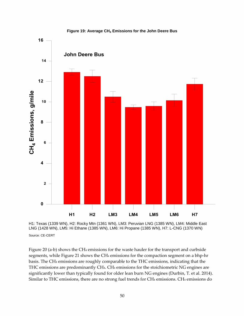
50

Figure 19: Average CH4 Emissions for the John Deere Bus


Source: CE-CERT

Figure 20 (a-b) shows the CH4 emissions for the waste hauler for the transport and curbside

segments, while Figure 21 shows the CH4 emissions for the compaction segment on a bhp-hr

basis. The CH4 emissions are roughly comparable to the THC emissions, indicating that the

THC emissions are predominantly CH4. CH4 emissions for the stoichiometric NG engines are

significantly lower than typically found for older lean burn NG engines (Durbin, T. et al. 2014).

Similar to THC emissions, there are no strong fuel trends for CH4 emissions. CH4 emissions do

51

not show any statistically significant differences between fuels for the transport cycle. For the

curbside cycle, the only statistically significant decrease is seen for LM3 (34 percent) compared

to H1. Although there are no large fuel differences, there is a trend showing higher CH4

emissions for the curbside cycle for H1 and H7, which are the two fuels with the higher levels of

CH4 in the test fuels. The compaction cycle did not show any statistically significant differences

for CH4 emissions.

Figure 20 (a-b): Average CH4 Emissions for Waste Hauler Transport and Curbside Segments


Source: CE-CERT

52

Figure 21: Average CH4 Emissions for Waste Hauler for the Compaction Segment on an Engine bhp-hr Basis


Source: CE-CERT

Figure 22 presents the CH4 emissions for the Cummins Westport ISL G (A) truck and Cummins

Westport ISX12 G (B) truck over the Near Dock duty cycle and the Local Haul duty cycle,

respectively. The results show that the Cummins Westport ISL G truck CH4 emissions were

about two times higher than those for the Cummins Westport ISX12 G truck. For both trucks the

highest CH4 emissions were seen for the creep phase and the lowest CH4 emissions were seen

for the high speed phase.

53

For the Cummins Westport ISL G truck, the accumulated CH4 emissions show statistically

significant decreases of 25.6 percent and 12.4 percent for LM5 and LM6, respectively, compared

to H1. For the creep phase, LM5 shows a statistically significant decrease in CH4 emissions of

42.3 percent relative to H1, while for the low speed transient phase both LM5 and LM6 show

statistically significant decreases of 36.5 percent and 26.5 percent, respectively, compared to H1.

For the Cummins Westport ISX12 G truck, the accumulated CH4 emissions show a statistically

significant increase of 19.2 percent for H7 compared to H1, while statistically significant

reductions in accumulated CH4 emissions of 16.1 percent, 23.1 percent, and 22.6 percent for H1,

LM4, and LM5, respectively, compared to H7 were also observed. For the low speed transient

phase, CH4 emissions show statistically significant decreases of 22.9 percent and 21.5 percent,

respectively, for LM4 and LM5 compared to H1 and of 31.4 percent and 30.1 percent,

respectively, compared to H7. For the long high-speed transient phase, CH4 emissions show a

statistically significant increase of 31.5 percent for LM5 and a marginally statistically significant

increase of 23.3 percent compared to H1.

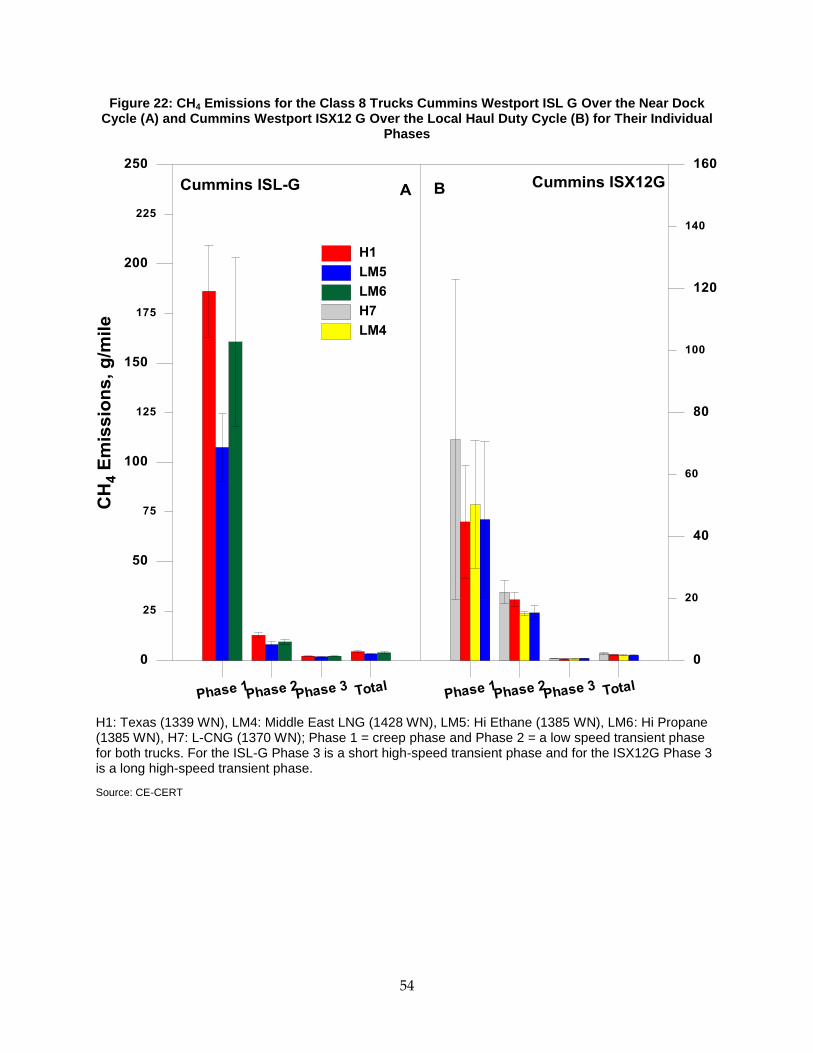
54

Figure 22: CH4 Emissions for the Class 8 Trucks Cummins Westport ISL G Over the Near Dock Cycle (A) and Cummins Westport ISX12 G Over the Local Haul Duty Cycle (B) for Their Individual

Phases


Source: CE-CERT

55

3.5 Carbon Monoxide Emissions

Figure 23 shows CO emissions for the John Deere school bus over the CBD cycle. The CO

emissions for the John Deere school bus were at very low levels, close to the measurement

background. For the CO emissions, there are no strong effects between the test fuels.

Figure 23: Average CO Emissions for the John Deere Bus


Source: CE-CERT

Figure 24 (a-b) shows the CO emissions for the waste hauler for the transport and curbside

segments, while Figure 25 shows the CO emissions for the compaction segment on a bhp-hr

basis. The CO emissions for the stoichiometric Cummins Westport ISL-G engine are higher

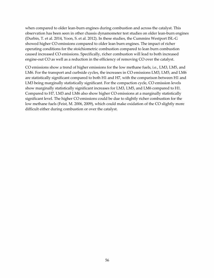
56

when compared to older lean-burn engines during combustion and across the catalyst. This

observation has been seen in other chassis dynamometer test studies on older lean-burn engines

(Durbin, T. et al. 2014, Yoon, S. et al. 2012). In these studies, the Cummins Westport ISL-G

showed higher CO emissions compared to older lean burn engines. The impact of richer

operating conditions for the stoichiometric combustion compared to lean burn combustion

caused increased CO emissions. Specifically, richer combustion will lead to both increased

engine-out CO as well as a reduction in the efficiency of removing CO over the catalyst.

CO emissions show a trend of higher emissions for the low methane fuels, i.e., LM3, LM5, and

LM6. For the transport and curbside cycles, the increases in CO emissions LM3, LM5, and LM6

are statistically significant compared to both H1 and H7, with the comparison between H1 and

LM3 being marginally statistically significant. For the compaction cycle, CO emission levels

show marginally statistically significant increases for LM3, LM5, and LM6 compared to H1.

Compared to H7, LM3 and LM6 also show higher CO emissions at a marginally statistically

significant level. The higher CO emissions could be due to slightly richer combustion for the

low methane fuels (Feist, M. 2006, 2009), which could make oxidation of the CO slightly more

difficult either during combustion or over the catalyst.

57

Figure 24 (a-b): Average CO Emissions for Waste Hauler Transport and Curbside Segments


Source: CE-CERT

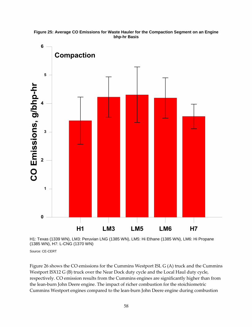
58

Figure 25: Average CO Emissions for Waste Hauler for the Compaction Segment on an Engine bhp-hr Basis


Source: CE-CERT

Figure 26 shows the CO emissions for the Cummins Westport ISL G (A) truck and the Cummins


respectively. CO emission results from the Cummins engines are significantly higher than from

the lean-burn John Deere engine. The impact of richer combustion for the stoichiometric

Cummins Westport engines compared to the lean-burn John Deere engine during combustion

59

and across the catalyst caused the higher CO emissions. This observation is consistent with the

results of previous chassis dynamometer tests as well as a recent engine dynamometer study

that evaluated Cummins Westport ISL, C-Gas Plus, C-Gas, and John Deere engines (Feist, M.

2009, Einewall, P. et al. 2005, Feist,M. et al. 2010, Yoon, S. et al. 2012). In these studies, the

Cummins Westport ISL G also shows the highest CO emissions compared to the other engines.

The CO emissions for the Cummins Westport ISL G truck and the Cummins Westport ISX12

truck were roughly comparable over the Near Dock and Local Haul Duty cycles.

For the Cummins Westport ISL G truck, the accumulated CO emissions show statistically

significant increases of 111.1 percent and 140.8 percent, respectively for LM5 and LM6

compared to H1. For the low speed transient phase, CO emissions show marginally statistically

significant increases of 377.7 percent and 285.1 percent, respectively, for LM5 and LM6

compared to H1. For the short high-speed transient phase, CO emissions show statistically

significant increases of 112.5 percent and 143.7 percent for LM5 and LM6, respectively,

compared to H1.

For the Cummins Westport ISX12 G truck, the accumulated CO emissions show statistically

significant increases of 41.5 percent and 60.3 percent, respectively, for the LM4 and LM5 low

methane fuels compared to H1 and of 36.1 percent and 54.2 percent, respectively, compared to

H7. For the creep phase, although the measurement variability is very large, CO emissions do

show a marginally statistically significant increase of 497 percent for LM4 compared to H1. For

the low speed transient phase, CO emissions show statistically significant increases of 123.2

percent and 141.1 percent, respectively, for LM4 and LM5 compared to H1 and of 54.9 percent

for LM5 compared to H7. For the long high-speed transient phase, CO emissions show

statistically significant increases for LM4 and LM5 of 37.3 percent and 51.8 percent, respectively,

compared to H1 and of 39.8 percent and 54.6 percent, respectively, compared to H7.

60

Figure 26: CO Emissions for the Class 8 Trucks Cummins Westport ISL G Over the Near Dock Cycle (A) and Cummins Westport ISX12 G Over the Local Haul Duty Cycle (B) for Their Individual

Phases


Source: CE-CERT

61

3.6 Fuel Economy and Carbon Dioxide Emissions

Figure 27 shows the average volumetric fuel economy in miles/ft3 for the John Deere school bus

over the CBD cycle. The formulas used to calculate the volumetric fuel economy and the energy

equivalent fuel economy are provided in Appendix C. Fuel economy is determined using the

carbon balance method. This method uses the amount of carbon emitted in the exhaust based

on THC, CO, and CO2 emissions to calculate how much fuel and fuel carbon the engine uses

during operation. As shown in Figure 27, the differences between the various test fuel

economies are readily apparent, and in many cases statistically significant, as discussed below.

The low methane fuels with the higher heating values, i.e., LM3, LM4, LM5, and LM6, show

higher fuel economy compared to H1, H2, and H7. The fuel economy increases for LM3, LM4,

LM5, and LM6 compared to H1 are all statistically significant for the school bus over the CBD

cycle, and were on the order of 4 percent, 9.3 percent, 8.1 percent, and 8.3 percent, respectively,

relative to H1, with H7 also showing a 1.7 percent increase in fuel economy at a statistically

significant level. The same trend also occurs for the low methane fuels when compared to H2,

with the increases being statistically significant and on the order of 3.7 percent to 9 percent.

Compared to H7, all test fuels show statistically significant differences in fuel economy with the

exception of H2. The low methane fuels show increases ranging from 2.2 percent to 7.5 percent,

while H1 decreases by 1.7 percent.

62

Figure 27: Average Volumetric Fuel Economy for the John Deere Bus


Source: CE-CERT

In using an energy equivalent basis for fuel economy, the energy differences between the fuels

are normalized. The normalized fuels eliminated the energy differences between fuels to

provide a more accurate fuel economy evaluation. Figure 28 presents the fuel economy results

for the John Deere school bus using the different fuel blends over the CBD test cycle on a

gasoline gallon equivalent (GGE) energy basis. The John Deere bus shows comparable fuel

economy results between fuels on an energy equivalent basis. Fuel economy does not show

63

significant fuel effects with the exception of H7, which shows a statistically significant increase

of 1.4 percent compared to H1.

Figure 28: Average Energy Equivalent Fuel Economy for the John Deere Bus


Source: CE-CERT

Figure 29 (a-b) shows the average volumetric fuel economy, respectively, in miles/ft3 for the

waste hauler truck (the transport and curbside segments). Figure 30 shows the volumetric fuel

consumption for the waste hauler on a ft3/bhp-hr basis. The formulas used to calculate the

volumetric and energy equivalent fuel economies, as discussed below, are provided in

Appendix C. Fuel economy was determined using the carbon balance method. Figure 29 (a-b)

64

and Figure 30 show that various test fuels have differences in fuel economies when fuel

economy and consumption are plotted on a volumetric basis. For the transport cycle,

statistically significant differences are seen with higher fuel economy for LM3, LM5, and LM6

compared to H1, while LM5 and LM6 show statistically significant and LM3 show marginally

statistically significant higher fuel economy compared to H7. The average fuel consumptions for

fuels LM3, LM5, and LM6 compared to H1 and H7 are also lower at a statistically significant

level for the compaction cycle. These trends are consistent with the fuels with the higher energy

content providing higher fuel economy and lower fuel consumption. For the curbside cycle, the

only marginally statistically significant and statistically significant differences in fuel economy

are higher fuel economy for LM3, LM5 and LM6 compared to H7. The same trends are seen for

the legacy waste hauler tested in Phase 1. For this vehicle, the low methane fuels show higher

volumetric fuel economy compared to H1, H2, and H7 over the transport and curbside phases

of the RTC, while the volumetric fuel consumption is lower for the low methane fuels,

consistent with the high energy contents of these fuels (Durbin, T. et al. 2014).

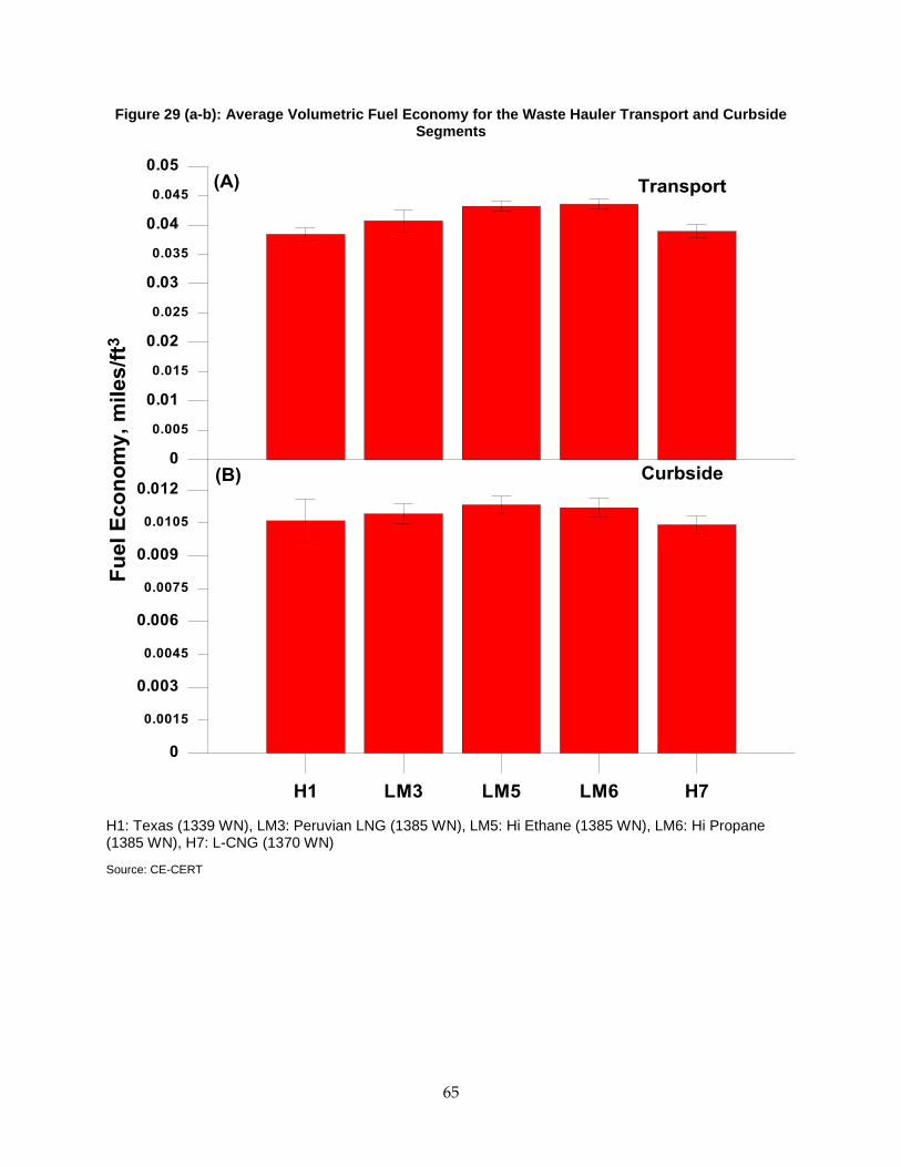
65

Figure 29 (a-b): Average Volumetric Fuel Economy for the Waste Hauler Transport and Curbside Segments


Source: CE-CERT

66

Figure 30: Average Volumetric Fuel Consumption for the Waste Hauler for the Compaction Segment on an Engine bhp-hr Basis


Source: CE-CERT

Fuel economy on an energy equivalent basis is shown in Figure 31 (a-b) on a gasoline gallon

equivalent (GGE) energy basis for the waste hauler for the transport and curbside segments. For

the waste hauler, fuel consumption is shown in Figure 32 on a gasoline gallon equivalent

energy basis for the compaction segment on a bhp-hr basis. The waste hauler does not show any

statistically significant trends in fuel economy or fuel consumption on an energy equivalent

basis, with the exception of LM6, which shows a statistically significant increase in fuel

67

consumption relative to H1 for the transport phase. The Phase 1 testing on the legacy waste

hauler shows stronger trends in fuel economy on an energy equivalent basis over the RTC

(Durbin, T. et al. 2014), with the low methane fuels with higher energy contents showing higher

energy equivalent fuel economy/lower fuel consumption compared to the high methane fuels.

Figure 31 (a-b): Average Energy Equivalent Fuel Economy for the Waste Hauler Transport and Curbside Segments


Source: CE-CERT

68

Figure 32: Average Energy Equivalent Fuel Consumption for the Waste Hauler for the Compaction Segment on an Engine bhp-hr Basis


Source: CE-CERT

Volumetric fuel economy in miles/ft3 for the Cummins Westport ISL G (A) truck and Cummins

Westport ISX12 G (B) truck over the Near Dock duty cycle and Local Haul duty cycle,

respectively, is shown in Figure 33. The volumetric fuel economy for these two trucks was

roughly comparable over the Near Dock and Local Haul Duty Cycles. The highest volumetric

fuel economy was found for the high speed transient phase and the lowest volumetric fuel

economy was observed for the creep phase.

69

For the Cummins Westport ISL G truck, the accumulated average volumetric fuel economy

shows statistically significant increases of 10.4 percent and 11.5 percent, respectively, for LM5

and LM6 compared to H1. For the creep phase, fuel economy shows a statistically significant

increase of 23.4 percent for LM5 compared to H1, while for the low speed transient phase both

LM5 and LM6 are higher on the order of 10.5 percent and 10.3 percent, respectively, compared

to H1 at a statistically significant level. For the short high-speed transient phase, the LM5 and

LM6 low methane fuels show statistically significant increases in fuel economy of 10.7 percent

and 11.9 percent, respectively, compared to H1. For the Cummins Westport ISX12 G truck, the

accumulated fuel economy shows statistically significant increases of about 12 percent for both

LM4 and LM5 and a marginally statistically significant increase of 4.2 percent for H7 compared

to H1. For the low speed transient phase, fuel economy shows statistically significant increases

of 13.8 percent and 8.5 percent, respectively for LM4 and LM5 compared to H1. For the long

high-speed transient phase, fuel economy shows statistically significant increases of 11.7

percent, 13.2 percent, and 5.3 percent for LM4, LM5, and H7, respectively, compared to H1.

Compared to H7, all test fuels show statistically significant differences in fuel economy.

Compared to H7, LM4 and LM5 show statistically significant increases of 6.1 percent and 7.5

percent, respectively, while H1 shows a statistically significant decrease of 5 percent.

70

Figure 33: Volumetric Fuel Economy for the Class 8 Trucks Cummins Westport ISL G Over the Near Dock Cycle (A) and Cummins Westport ISX12 G Over the Local Haul Duty Cycle (B) for Their

Individual Phases


Source: CE-CERT

Figure 34 shows the fuel economy results for the Cummins Westport trucks on an energy

equivalent basis. Fuel economy on a gasoline gallon equivalent (GGE) energy basis do not show

any strong trends between the test fuels for the Cummins Westport ISL G truck over the Near

Dock duty cycle and its individual phases. The energy-equivalent fuel economy for these two

trucks was roughly comparable over the Near Dock and Local Haul Duty Cycles. The highest

energy-equivalent fuel economy was found for the high-speed transient phase and the lowest

71

energy equivalent fuel economy was observed for the creep phase. The only statistically

significant effect is seen for the LM6 low methane fuel, which shows an increase of 2 percent

compared to H1 at a marginally statistically significant level during the short high-speed

transient phase. For the Cummins Westport ISX12 G truck, accumulated fuel economy on an

energy equivalent basis shows a marginally statistically significant increase of 2.7 percent for

LM5 compared to H1. For the long high-speed transient phase, LM5 also shows a marginally

statistically significant increase of 3.3 percent compared to H1. Overall, for both Cummins

Westport trucks, the low methane fuels with higher energy contents exhibit higher energy-

equivalent fuel economy compared to the H1.

Figure 34: Energy Equivalent Fuel Consumption for the Class 8 Trucks Cummins Westport ISL G Over the Near Dock Cycle (A) and Cummins Westport ISX12 G Over the Local Haul Duty Cycle (B)

for Their Individual Phases


Source: CE-CERT

72

For the John Deere school bus, CO2 emissions over the CBD cycle are shown in Figure 35. The

CO2 emissions do not show strong trends between the test fuels over the CBD cycle, with the

exception of H7, which shows a statistically significant decrease of 2.3 percent in CO2 emissions

compared to H1. Compared to H7, most test fuels show statistically significant increases in CO2

emissions ranging from 2.3 percent to 3.5 percent, with the exception of H2.

Figure 35: Average CO2 Emissions for the John Deere Bus


Source: CE-CERT

CO2 emissions for the waste hauler are shown in Figure 36 (a-b) for the transport and curbside

segments. For the curbside segment, CO2 emissions are higher than those for the transport

segment on a per mile basis. No statistically significant fuel effects are found for either the

73

transport or curbside cycles. CO2 emissions for the waste hauler are shown in Figure 37 for the

compaction segment on a bhp-hr basis. For the compaction segment, there is a statistically

significant reduction for H7 compared to LM3, LM5, and a marginally statistically significant

reduction compared to LM6. H7 does have a higher hydrogen to carbon (H/C) ratio than LM3,

LM5, and LM6, so the reduction in CO2 emissions is consistent with a lower carbon fraction in

the fuel, although the H/C is similar to that for H1, which does not show any significant fuel

trends. The results for this waste hauler are similar to those for the legacy waste hauler for the

compaction phase, with CO2 emissions being higher for the low methane fuels compared to H1,

H2, and H7 (Durbin, T. et al. 2014). The legacy vehicle shows stronger reduction trends in CO2

emissions for the transport cycle, showing some statistically significant reductions for the low

methane fuels compared to H1 and H2, but not H7.

Figure 36 (a-b): Average CO2 Emissions for the Waste Hauler Transport and Curbside Segments


Source: CE-CERT

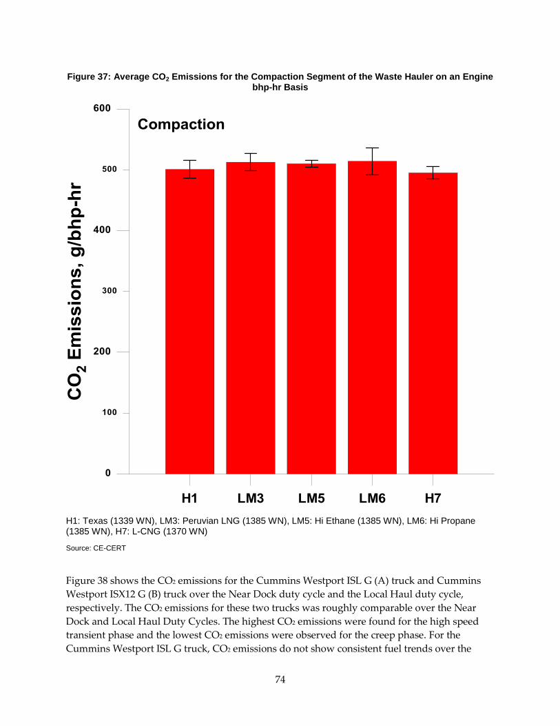
74

Figure 37: Average CO2 Emissions for the Compaction Segment of the Waste Hauler on an Engine bhp-hr Basis


Source: CE-CERT

Figure 38 shows the CO2 emissions for the Cummins Westport ISL G (A) truck and Cummins


respectively. The CO2 emissions for these two trucks was roughly comparable over the Near

Dock and Local Haul Duty Cycles. The highest CO2 emissions were found for the high speed

transient phase and the lowest CO2 emissions were observed for the creep phase. For the

Cummins Westport ISL G truck, CO2 emissions do not show consistent fuel trends over the

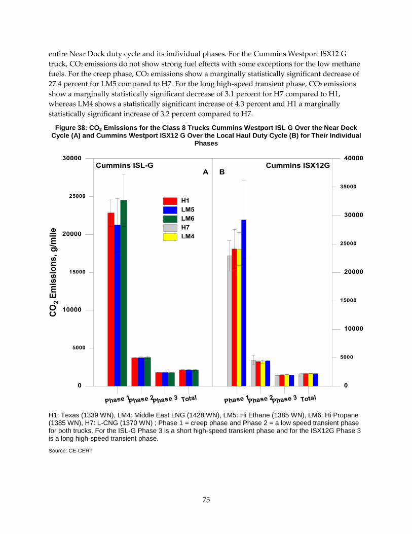
75

entire Near Dock duty cycle and its individual phases. For the Cummins Westport ISX12 G

truck, CO2 emissions do not show strong fuel effects with some exceptions for the low methane

fuels. For the creep phase, CO2 emissions show a marginally statistically significant decrease of

27.4 percent for LM5 compared to H7. For the long high-speed transient phase, CO2 emissions

show a marginally statistically significant decrease of 3.1 percent for H7 compared to H1,

whereas LM4 shows a statistically significant increase of 4.3 percent and H1 a marginally

statistically significant increase of 3.2 percent compared to H7.

Figure 38: CO2 Emissions for the Class 8 Trucks Cummins Westport ISL G Over the Near Dock Cycle (A) and Cummins Westport ISX12 G Over the Local Haul Duty Cycle (B) for Their Individual

Phases

H1: Texas (1339 WN), LM4: Middle East LNG (1428 WN), LM5: Hi Ethane (1385 WN), LM6: Hi Propane (1385 WN), H7: L-CNG (1370 WN) ; Phase 1 = creep phase and Phase 2 = a low speed transient phase for both trucks. For the ISL-G Phase 3 is a short high-speed transient phase and for the ISX12G Phase 3 is a long high-speed transient phase.

Source: CE-CERT

76

3.7 Particulate Matter Mass Emissions

Figure 39 shows the PM mass emissions for the John Deere school bus over the CBD cycle. The

results indicate that total PM mass emissions are low for the lean-burn John Deere engine on an

absolute level, and in some cases close to the background levels. During testing with the John

Deere engine, there were differences seen in PM mass emissions, some of which could be

attributed to fuel effects and other differences in PM mass emissions are within the range of the

tunnel background levels. PM mass emissions show a marginally statistically significant

increase of 95 percent for H2 and a statistically significant increase of 217 percent for LM3

compared to H1. Compared to H2, PM mass emissions show a statistically significant increase

of 63 percent for LM3 and a statistically significant reduction of 78 percent for LM5 is also

observed. PM mass emissions are also statistically significantly higher for LM3 relative to H7.

77

Figure 39: Average PM Emissions for the John Deere Bus


Source: CE-CERT

PM mass emissions for the waste hauler are shown in Figure 40 for the composite Refuse Truck

Cycle. As explained in the experimental section, PM emissions were collected cumulatively over

the entire duration of the RTC due to the expectation of low mass levels emitted; therefore,

separate emissions are not available for the curbside, transport, and compaction segments.

Instead, PM emissions are shown in terms of g/cycle.

The results indicated that total PM mass emissions were very low for the refuse truck on an

absolute level. Although some differences were seen between fuels, these differences were all

78

within the experimental variability. As a result, there were essentially no differences between

PM mass for different fuels.

The very low levels of PM mass emissions found in the tailpipe result from combustion that

generates low PM levels and as well as the reduction of PM with the TWC. Both the natural gas

fuel combustion and the lubricant oil leakage into the combustion chamber generated PM.

Natural gas is primarily comprised of methane, which is the lowest molecular weight

hydrocarbon and a simpler structure compared to diesel and gasoline fuels (Walkowicz, K. et al.

2003). Natural gas has a reduced tendency to form localized areas of rich combustion and

generates unburned and partially oxidized hydrocarbons with lower molecular sizes in the

exhaust, resulting in very low PM mass emission levels. The PM contribution from natural gas

combustion is expected to be smaller than from entry of the engine lubricant oil. Previous

studies have shown that lubricant-oil-based additives and wear metals were a major fraction of

the PM mass from NG buses (Thiruvengadam, A. et al. 2014). The low PM levels formed from

the combustion process are further reduced as the exhaust stream passes over the catalyst bed.

The carbon particles in the exhaust carry adsorbed water-soluble, organic PM compounds. The

catalyst bed oxidizes some of the soluble organic fraction (SOF) portion of PM to CO2 and

water.

Testing on the legacy waste hauler in Phase 1 showed higher PM mass emission levels than

those reported for the stoichiometric engine (Durbin, T. et al. 2014). Measured PM for the legacy

vehicle was in the 0.025 to 0.069 g/cycle range compared to 0.006 to 0.016 g/cycle for the

stoichiometric engine. The lower PM emissions for the stoichiometric engine compared to the

legacy 2005 lean-burn engine could be attributed to the fact that the stoichiometric engine is

designed to meet more stringent emissions standards than the legacy engine, or perhaps a

reduction in lubricant oil consumption for the newer stoichiometric engine. Unlike the results

reported here, the legacy vehicle exhibited statistically significant reductions in PM mass

emissions for the low methane fuels compared to high methane fuels (Durbin, T. et al. 2014).

The PM levels for the stoichiometric engine, which are lower than those for the legacy engine,

are near the background levels. At such levels, the experimental variability becomes greater on

an absolute basis, making it more difficult to measure differences between fuels.

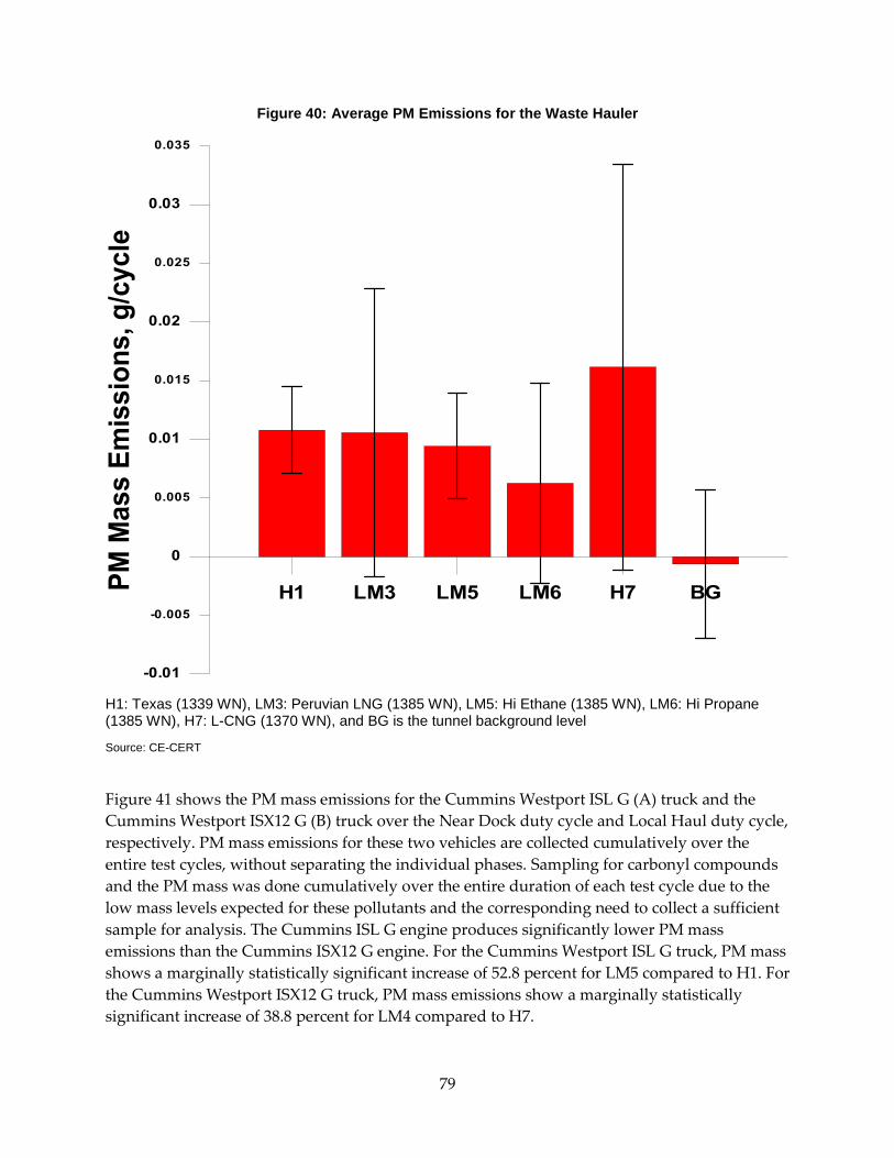
79

Figure 40: Average PM Emissions for the Waste Hauler

H1: Texas (1339 WN), LM3: Peruvian LNG (1385 WN), LM5: Hi Ethane (1385 WN), LM6: Hi Propane (1385 WN), H7: L-CNG (1370 WN), and BG is the tunnel background level

Source: CE-CERT

Figure 41 shows the PM mass emissions for the Cummins Westport ISL G (A) truck and the

Cummins Westport ISX12 G (B) truck over the Near Dock duty cycle and Local Haul duty cycle,

respectively. PM mass emissions for these two vehicles are collected cumulatively over the

entire test cycles, without separating the individual phases. Sampling for carbonyl compounds

and the PM mass was done cumulatively over the entire duration of each test cycle due to the

low mass levels expected for these pollutants and the corresponding need to collect a sufficient

sample for analysis. The Cummins ISL G engine produces significantly lower PM mass

emissions than the Cummins ISX12 G engine. For the Cummins Westport ISL G truck, PM mass

shows a marginally statistically significant increase of 52.8 percent for LM5 compared to H1. For

the Cummins Westport ISX12 G truck, PM mass emissions show a marginally statistically

significant increase of 38.8 percent for LM4 compared to H7.

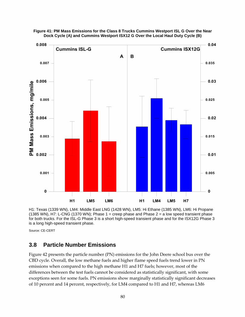
80

Figure 41: PM Mass Emissions for the Class 8 Trucks Cummins Westport ISL G Over the Near Dock Cycle (A) and Cummins Westport ISX12 G Over the Local Haul Duty Cycle (B)


Source: CE-CERT

3.8 Particle Number Emissions

Figure 42 presents the particle number (PN) emissions for the John Deere school bus over the

CBD cycle. Overall, the low methane fuels and higher flame speed fuels trend lower in PN

emissions when compared to the high methane H1 and H7 fuels; however, most of the

differences between the test fuels cannot be considered as statistically significant, with some

exceptions seen for some fuels. PN emissions show marginally statistically significant decreases

of 10 percent and 14 percent, respectively, for LM4 compared to H1 and H7, whereas LM6

81

shows a statistically significant increase in PN emissions of 21 percent compared to H2. PN

emissions for this vehicle were much higher than those emissions tested for the stoichiometric

engine vehicles tested for this study and the 2004 lean-burn John Deere bus tested in a previous

CE-CERT study (Hajbabaei, M. 2013).

Figure 42: Average PN Emissions for the John Deere Bus


Source: CE-CERT

For the waste hauler, PN emissions are shown in Figure 43 (a-b) for the transport and curbside

segments and in Figure 44 for the compaction segment on a bhp-hr basis. PN emissions do not

show strong fuel trends for either the transport or the curbside segments of the RTC. The

transport segment is the only segment where statistically significant differences are observed

between fuels. PN emissions show a marginally statistically significant increase of 17.4 percent

for LM6 compared to H1. LM5 and LM6 show statistically significant increases in PN emissions

82

of 26.5 percent and 37.0 percent, respectively, while LM3 shows a marginally statistically

significant increase of 18.8 percent compared to H7. PN emissions are approximately an order

of magnitude higher for the curbside segment compared to the transport segment of the cycle,

as the curbside segment covers a much shorter distance and is primarily composed of low speed

accelerations and idling periods with little steady state driving. For the compaction segment,

there are no statistically significant differences between the test fuels.

In comparing the results obtained from this study to previous work conducted by CE-CERT

(Durbin, T. et al. 2014), the similarity in total PN emissions between older and newer technology

natural gas engines suggests that PN emissions are largely attributed to lubricant oil and not the

changes in the fuel combustion and of after treatment type.

83

Figure 43: Average PN Emissions for Waste Hauler


Source: CE-CERT

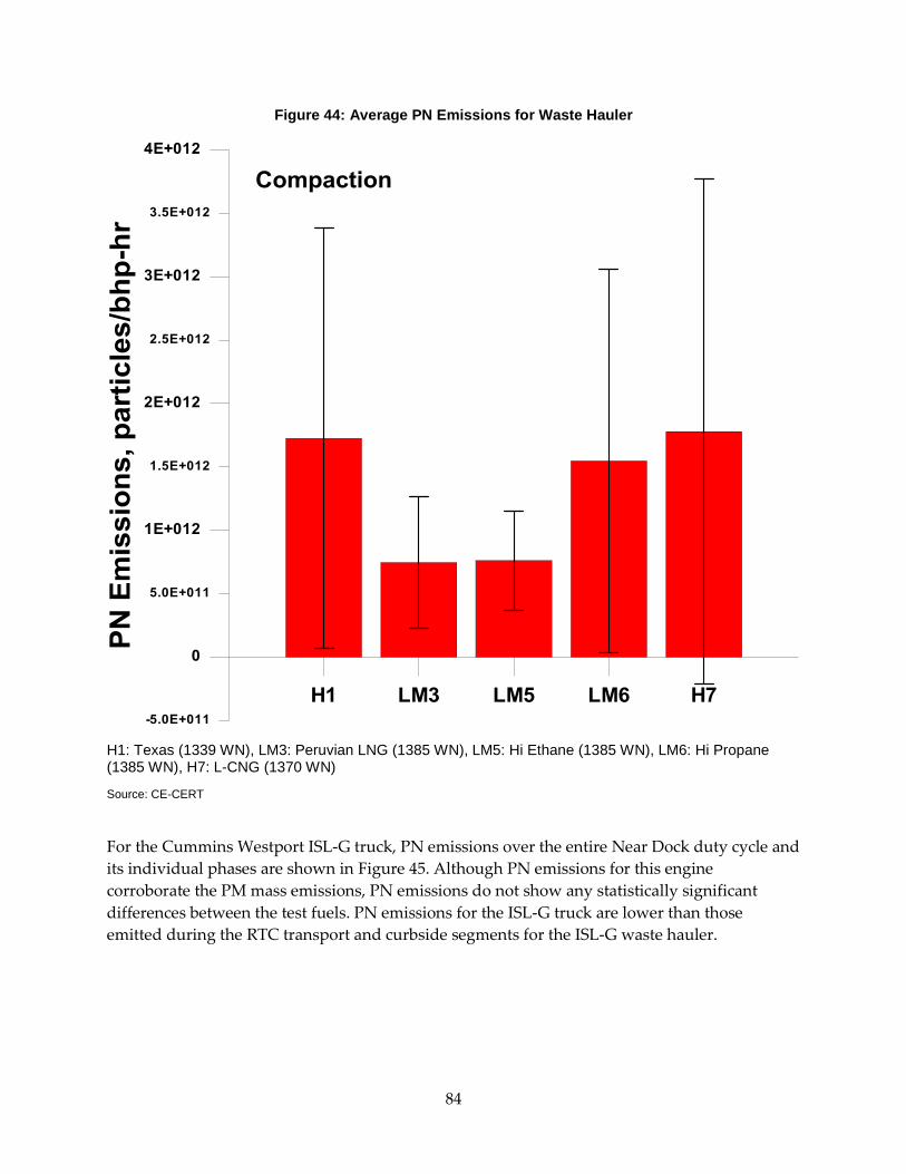
84

Figure 44: Average PN Emissions for Waste Hauler


Source: CE-CERT

For the Cummins Westport ISL-G truck, PN emissions over the entire Near Dock duty cycle and

its individual phases are shown in Figure 45. Although PN emissions for this engine

corroborate the PM mass emissions, PN emissions do not show any statistically significant

differences between the test fuels. PN emissions for the ISL-G truck are lower than those

emitted during the RTC transport and curbside segments for the ISL-G waste hauler.

85

Figure 45: PN Emissions for the Cummins Westport ISL-G Truck (Near Dock Cycle)

H1: Texas (1339 WN), LM5: Hi Ethane (1385 WN), LM6: Hi Propane (1385 WN); Phase 1 = creep phase, Phase 2 = a low speed transient phase, and Phase 3 = a short high-speed transient phase.

Source: CE-CERT

For the Cummins Westport ISX12G truck, PN emissions over the Local Haul duty cycle and its

individual phases are shown in Figure 46. Emissions of PN for the entire cycle and its

individual phases are higher for this vehicle than the Cummins ISL-G truck and the ISL-G waste

hauler, but lower than the lean-burn John Deere bus. The low methane fuels, i.e., LM4 and LM5

show statistically significant increases in PN emissions of 46.5 percent and 31.7 percent,

respectively, compared to H1 for the long high-speed transient phase 3. The accumulated PN

emissions also show a statistically significant increase of 52.7 percent for LM4 compared to H1.

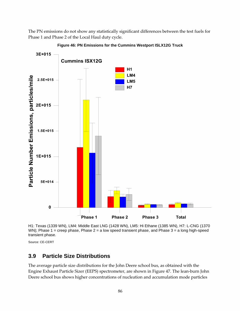
86

The PN emissions do not show any statistically significant differences between the test fuels for

Phase 1 and Phase 2 of the Local Haul duty cycle.

Figure 46: PN Emissions for the Cummins Westport ISLX12G Truck

H1: Texas (1339 WN), LM4: Middle East LNG (1428 WN), LM5: Hi Ethane (1385 WN), H7: L-CNG (1370 WN); Phase 1 = creep phase, Phase 2 = a low speed transient phase, and Phase 3 = a long high-speed transient phase.

Source: CE-CERT

3.9 Particle Size Distributions

The average particle size distributions for the John Deere school bus, as obtained with the

Engine Exhaust Particle Sizer (EEPS) spectrometer, are shown in Figure 47. The lean-burn John

Deere school bus shows higher concentrations of nucleation and accumulation mode particles

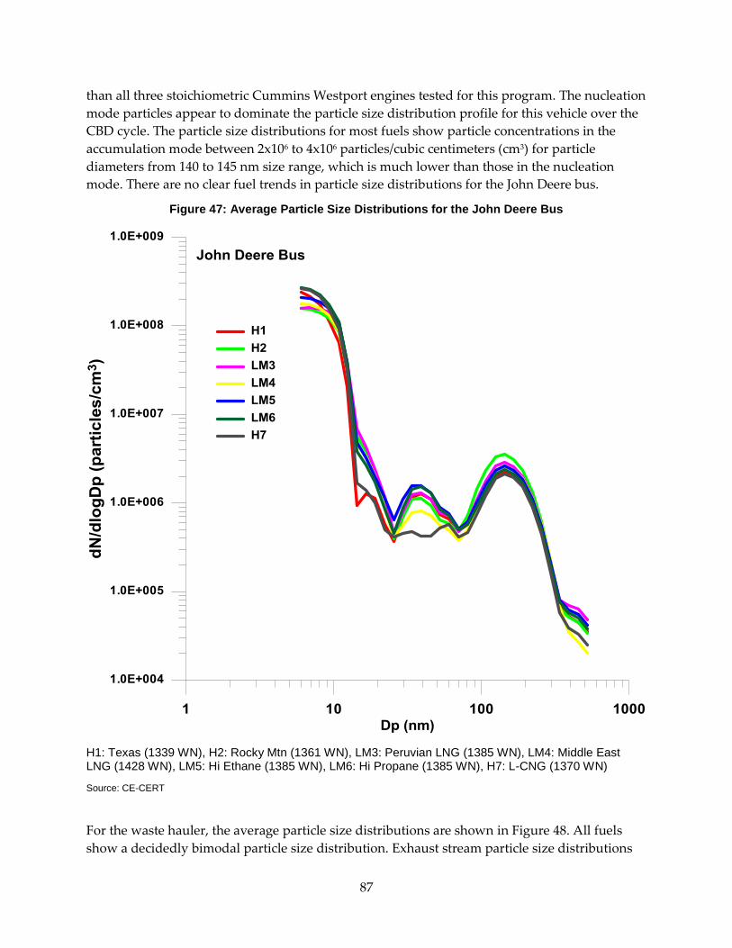
87

than all three stoichiometric Cummins Westport engines tested for this program. The nucleation

mode particles appear to dominate the particle size distribution profile for this vehicle over the

CBD cycle. The particle size distributions for most fuels show particle concentrations in the

accumulation mode between 2x106 to 4x106 particles/cubic centimeters (cm3) for particle

diameters from 140 to 145 nm size range, which is much lower than those in the nucleation

mode. There are no clear fuel trends in particle size distributions for the John Deere bus.

Figure 47: Average Particle Size Distributions for the John Deere Bus


Source: CE-CERT

For the waste hauler, the average particle size distributions are shown in Figure 48. All fuels

show a decidedly bimodal particle size distribution. Exhaust stream particle size distributions

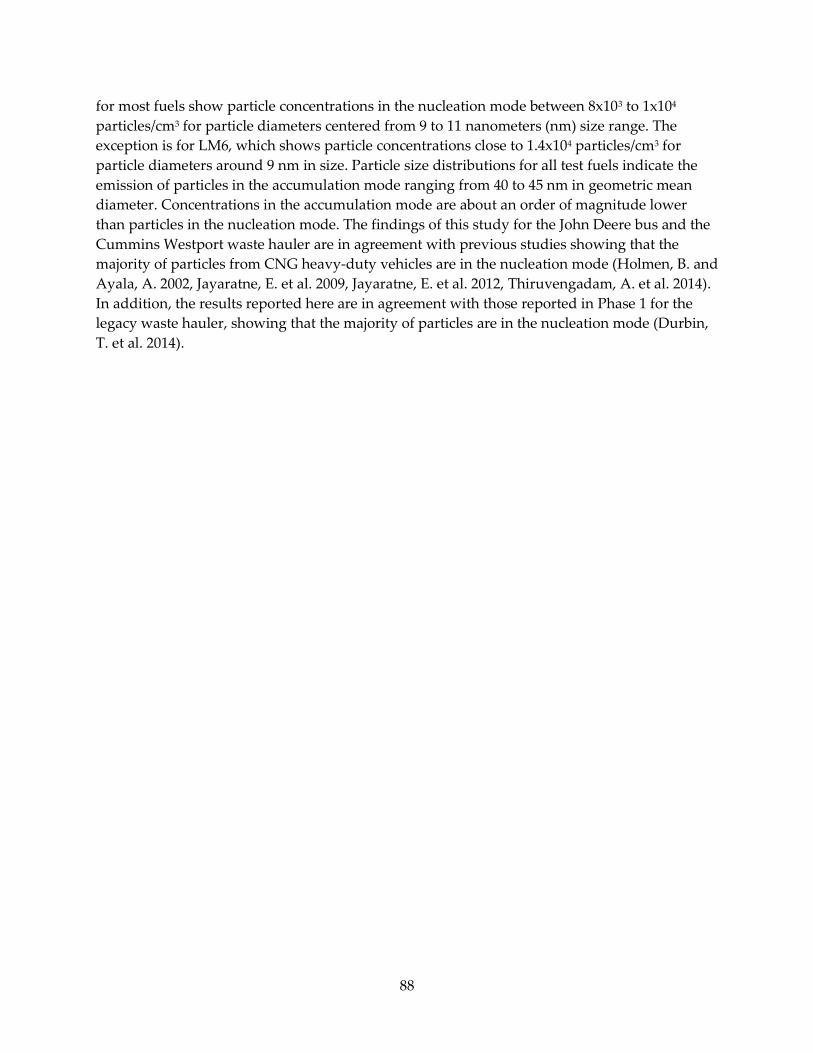
88

for most fuels show particle concentrations in the nucleation mode between 8x103 to 1x104

particles/cm3 for particle diameters centered from 9 to 11 nanometers (nm) size range. The

exception is for LM6, which shows particle concentrations close to 1.4x104 particles/cm3 for

particle diameters around 9 nm in size. Particle size distributions for all test fuels indicate the

emission of particles in the accumulation mode ranging from 40 to 45 nm in geometric mean

diameter. Concentrations in the accumulation mode are about an order of magnitude lower

than particles in the nucleation mode. The findings of this study for the John Deere bus and the

Cummins Westport waste hauler are in agreement with previous studies showing that the

majority of particles from CNG heavy-duty vehicles are in the nucleation mode (Holmen, B. and

Ayala, A. 2002, Jayaratne, E. et al. 2009, Jayaratne, E. et al. 2012, Thiruvengadam, A. et al. 2014).

In addition, the results reported here are in agreement with those reported in Phase 1 for the

legacy waste hauler, showing that the majority of particles are in the nucleation mode (Durbin,

T. et al. 2014).

89

Figure 48: Average Particle Size Distributions for the Waste Hauler


Source: CE-CERT

Figure 49 illustrates the particle size distributions for the Cummins Westport ISL-G truck over

the Near Dock duty cycle. Similar to the waste hauler, the ISL-G truck shows a decidedly

bimodal particle size distribution; however, the accumulation mode is the prevalent mode of

particle formation for this engine as opposed to the John Deere bus and waste hauler. This

finding is interesting since both the waste hauler and the truck are fitted with the same

Cummins Westport ISL-G 8.9L engine. The particle size distributions for the three test fuels

show particle concentrations in the nucleation mode from 5x103 to 8x103 particles/cm3 for

particle diameters centered from 9 to 10 nm size range. The highest concentrations in nucleation

90

mode particles are seen for the low methane fuels, i.e., LM5 and LM6, compared to H1. For the

accumulation mode particles, particle diameters ranging from 140 to 143 nm in size range with

particle concentrations from 8x103 to 10x104 particles/cm3. The high methane H1 fuel produces

higher concentrations of accumulation mode particles followed by LM5 and LM6. It should be

stressed that the ISL-G truck results in accumulation particles with larger diameters compared

to the ISL-G waste hauler.

Figure 49: Average Particle Size Distributions for the Cummins Westport ISL-G Truck

H1: Texas (1339 WN), LM5: Hi Ethane (1385 WN), LM6: Hi Propane (1385 WN)

Source: CE-CERT

For the Cummins Westport ISX12G truck, average particle-size distributions over the Local

Haul duty cycle are shown in Figure 50. Similar to the previous vehicles tested in this study, the

ISX12G truck shows a decidedly bimodal particle size distribution. Unlike the particle size

distribution profile for the ISL-G truck, but more similar to waste hauler and school bus, the

ISX12G truck produces higher concentrations of accumulation mode particles compared to the

nucleation mode particles. The particle size distributions for the test fuels show particle

concentrations in the nucleation mode from 6x108 to 10x1010 particles/cm3 for particle diameters

91

centered from 9 to 10 nm size range. The particle concentrations in the nucleation mode for the

ISX12G truck are considerably higher when compared to all three vehicles tested. For the

accumulation mode particles, particle concentrations are from 5x108 to 6x108 particles/cm3 for

particle diameters from 60 to 70 nm size range. Compared to ISL-G truck, the ISX12G truck

produces higher accumulation-mode particle counts with smaller diameters. For the ISX12G

truck, a fuel effect was noticeable with the low methane fuels showing higher accumulation and

nucleation-mode particle concentrations than H1 and H7.

In general, it is reasonable to theorize that the observed particle size distributions could be

attributed to in-cylinder combustion of lubricant oil, which contributed sulfates nucleating with

water to form sulfuric acid particles in the 10 nm peak size. Similar observations were reported

by Thiruvengadam et al. (2014) when they tested two 2007 CNG buses fitted with Cummins

ISLG280 engines and TWCs. The lubricant oil entry into the combustion chamber is dependent

on engine load. Typically low-load operations, such as those applied during the RTC for the

Cummins Westport waste hauler, result in insufficient piston ring sealing, which can contribute

to the combustion of lubricant oil (Yoon, S. et al. 2012). It is also reasonable to assume that the

low-load operation of RTC resulted in lower accumulation mode particles or soot emissions and

increased the probability of the formation of inorganic nucleation mode particles. The Cummins

ISL-G truck produced less accumulation particles when operated over the Near Dock duty cycle

compared to the Cummins ISX12G truck. This result could be due to the third phase of the Near

Dock duty cycle (short high-speed transient phase) where the vehicle is subjected to lower

speed and load conditions compared to the third phase of the Local Haul duty cycle (long high-

speed transient phase). Khalek et al. (1998) explained this phenomenon showing that lubricant

oil additives do undergo volatilization when passing through the combustion chamber and a

fraction of them renucleate to form nanoparticles.

92

Figure 50: Particle Size Distributions for the Cummins Westport ISX12G Truck

H1: Texas (1339 WN), LM4: Middle East LNG (1428 WN), LM5: Hi Ethane (1385 WN), H7: L-CNG (1370 WN)

Source: CE-CERT

3.10 Ammonia Emissions

Road traffic is a major source of reactive nitrogen compounds such as NH3. NH3 is involved in

the formation of secondary aerosols and considered as a toxic pollutant. Ammonia is formed de

novo in noble metal-based TWCs; therefore, is a secondary pollutant of the catalytic process

rather than a side product of the fuel combustion. NO and H2, both formed during combustion,

are the assumed precursor molecules (Bielaczyc, P. et al. 2012).

93

Figure 51 shows the NH3 emissions for the John Deere school bus over the CBD test cycle.

Emissions of NH3 are found to be at substantially lower levels for the lean-burn John Deere

vehicle compared to the stoichiometric engines, ranging from 27.5 mg/mile to 51.0 mg/mile. In

general, NH3 emissions show a declining trend for all test fuels compared to H1. Emissions of

NH3 show statistically significant reductions of 46.2 percent, 45.4 percent, and 40.6 percent for

H2, LM5, and H7, respectively, compared to H1. H1 shows statistically significant increases in

NH3 emissions of 85.7 percent compared to H2. Overall, NH3 emissions do not show consistent

fuel effects for the John Deere bus, since most of the differences were between the high methane

fuels.

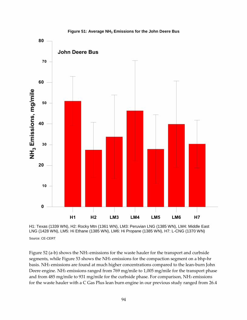
94

Figure 51: Average NH3 Emissions for the John Deere Bus


Source: CE-CERT

Figure 52 (a-b) shows the NH3 emissions for the waste hauler for the transport and curbside

segments, while Figure 53 shows the NH3 emissions for the compaction segment on a bhp-hr

basis. NH3 emissions are found at much higher concentrations compared to the lean-burn John

Deere engine. NH3 emissions ranged from 769 mg/mile to 1,005 mg/mile for the transport phase

and from 485 mg/mile to 931 mg/mile for the curbside phase. For comparison, NH3 emissions

for the waste hauler with a C Gas Plus lean burn engine in our previous study ranged from 26.4

95

mg/mile to 37.1 mg/mile and from 81.1 mg/mile to 115.9 mg/mile for the transport and curbside

phases, respectively (Durbin, T. et al. 2014). NH3 emissions are generally higher for the low

methane fuels, i.e., LM3, LM5, and LM6. The increases in NH3 emissions for LM3, LM5, and

LM6 are statistically significant compared to both H1 and H7 for all three of the test cycles.

For TWC-equipped stoichiometric natural gas engines, the production of NH3 takes place in the

presence of hydrogen molecules, which are produced during periods of rich air-fuel mixtures.

A water gas shift reaction involving CO and water or steam reforming reactions involving CH4

and water in the exhaust can form hydrogen (Majia-Centeno, I. et al. 2007, Huai, T. et al. 2003,

Gandhi, H. et al. 1974). It has been suggested that hydrogen produced in the water-gas shift

reaction (CO + H2O ↔ CO2 + H2) could be a major contributor to NH3 formation through the

overall reaction of 2NO + 2CO + 3H2 → 2NH3 + 2CO2. Fuel composition appears to have played

some role in NH3 emissions under the present test conditions. The higher NH3 emissions for the

low methane fuels could be due to slightly richer combustion (Feist, M. 2006). It is also known

that oxidation of methane with a standard TWC with platinum/palladium/rhodium is difficult

to achieve than oxidation of heavier components ethane and propane. Due to the lower

reactivity of CH4 over the TWC, an increase in the proportion of CH4 in the engine-out exhaust

gas flux would decrease the quantity of hydrogen available for ammonia formation. This CH4

reaction over the TWC could explain why there were lower ammonia emissions observed for

the high methane fuels compared to LM3, LM5, and LM6. The presence of higher CO levels also

facilitates the NH3 formation in the exhaust of a TWC-equipped stoichiometric natural gas

vehicle. Under the present test conditions, the low methane fuels showed higher CO emissions

over all three phases of the RTC resulting in higher NH3 emissions.

96

Figure 52 (a-b): Average NH3 Emissions for Waste Hauler Transport and Curbside Segments


Source: CE-CERT

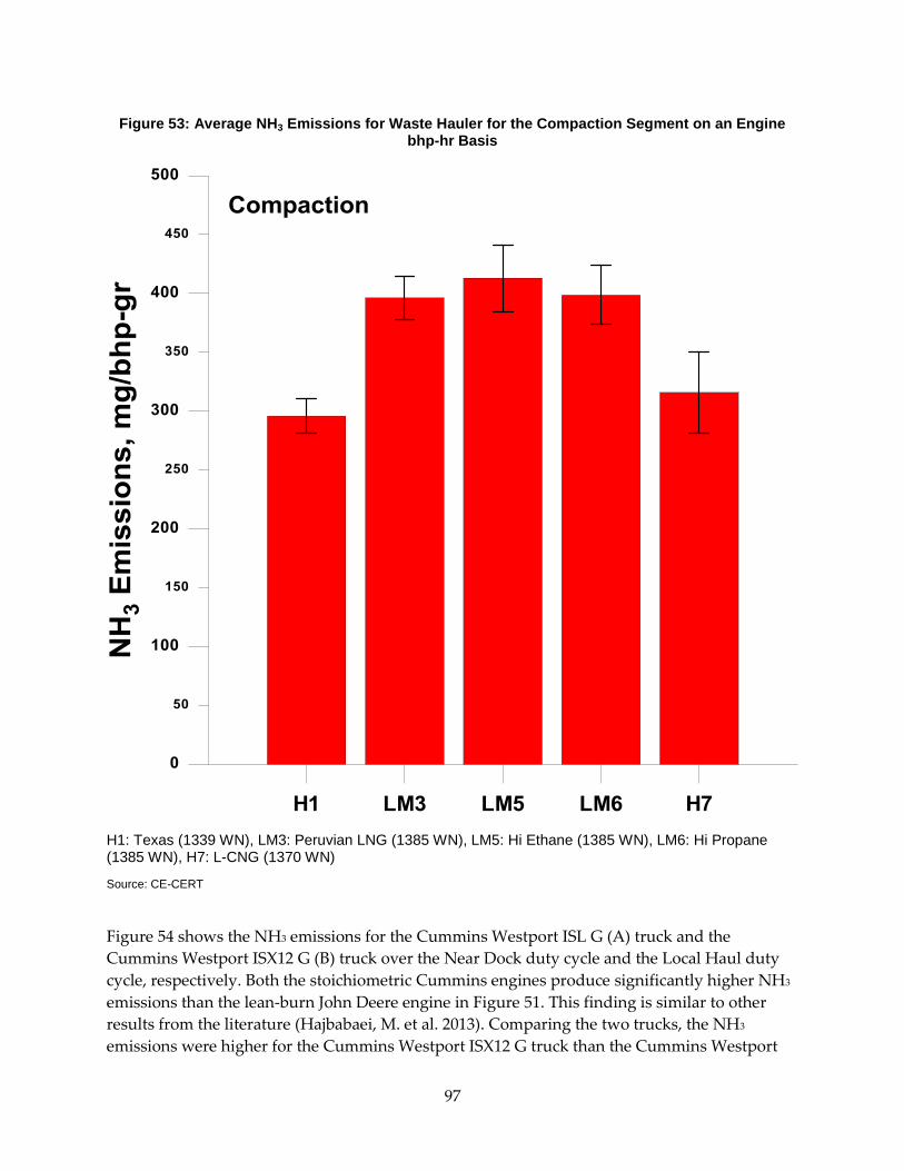
97

Figure 53: Average NH3 Emissions for Waste Hauler for the Compaction Segment on an Engine bhp-hr Basis


Source: CE-CERT

Figure 54 shows the NH3 emissions for the Cummins Westport ISL G (A) truck and the

Cummins Westport ISX12 G (B) truck over the Near Dock duty cycle and the Local Haul duty

cycle, respectively. Both the stoichiometric Cummins engines produce significantly higher NH3

emissions than the lean-burn John Deere engine in Figure 51. This finding is similar to other

results from the literature (Hajbabaei, M. et al. 2013). Comparing the two trucks, the NH3

emissions were higher for the Cummins Westport ISX12 G truck than the Cummins Westport

98

ISL G truck. Additionally, for both Cummins engines NH3 emissions are higher for the low

methane fuels, i.e., LM4, LM5, and LM6, compared to H1 and H7. The higher NH3 emissions for

the Cummins engines could be due to the fact that the low methane/higher Wobbe

number/higher flame speed fuels can produce higher exhaust temperatures and possibly

slightly richer air-fuel ratios. The conditions for the formation of hydrogen as a precursor and

NH3 as reaction product could be enhanced for the low methane fuels. Ammonia is a secondary

pollutant formed during the NOx reduction process over the TWC, with the formation

dependent to the presence of both nitrogen oxide (NO) and hydrogen (H2) in the exhaust

stream. For TWC-equipped stoichiometric natural gas engines, the production of NH3 takes

place in the presence of hydrogen molecules, which form during periods of rich air-fuel

mixtures. Hydrogen can also form from a water gas shift reaction involving CO and water or

steam reforming reactions involving CH4 and water in the exhaust (Majia-Centeno, I. et al. 2007,

Huai, T. et al. 2003, Gandhi, H. et al. 1974).

For the Cummins Westport ISL G truck, accumulated NH3 emissions show statistically

significant increases of 36.7 percent and 17.4 percent, respectively for LM5 and LM6 compared

to H1. For the low speed transient phase, NH3 emissions also show statistically significant

increases of 208.1 percent and 192.6 percent, respectively, for LM5 and LM6 compared to H1,

while for the short high-speed transient phase the LM5 low methane fuel showed an increase of

31.2 percent compared to H1 at a statistically significant level. For the Cummins Westport ISX12

G truck, accumulated NH3 emissions show statistically significant increases of 28.9 percent and

35.1 percent for LM4 and LM5, respectively, compared to H1, while LM5 also shows a

marginally statistically significant increase of 22.0 percent compared to H7. For the low speed

transient phase, NH3 emissions show statistically significant increases of 83.4 percent, 115.3

percent, and 94.6 percent for LM4, LM5, and H7, respectively, compared to H1; whereas, H1

shows a statistically significant reduction of 48.6 percent compared to H7. For the long high-

speed transient phase, NH3 emissions show statistically significant increases of 27.6 percent and

29.9 percent, respectively, for LM4 and LM5 compared to H1.

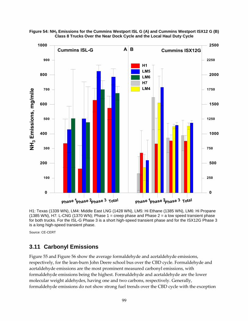
99

Figure 54: NH3 Emissions for the Cummins Westport ISL G (A) and Cummins Westport ISX12 G (B) Class 8 Trucks Over the Near Dock Cycle and the Local Haul Duty Cycle


Source: CE-CERT

3.11 Carbonyl Emissions

Figure 55 and Figure 56 show the average formaldehyde and acetaldehyde emissions,

respectively, for the lean-burn John Deere school bus over the CBD cycle. Formaldehyde and

acetaldehyde emissions are the most prominent measured carbonyl emissions, with

formaldehyde emissions being the highest. Formaldehyde and acetaldehyde are the lower

molecular weight aldehydes, having one and two carbons, respectively. Generally,

formaldehyde emissions do not show strong fuel trends over the CBD cycle with the exception

100

of LM3 and LM4 fuels, which show statistically significant increases of 14.8 percent and 11.6

percent, respectively, compared to H2 and 27.7 percent and 24.2 percent, respectively,

compared to H7. Formaldehyde emissions follow the same trends as the NMHC emissions,

with the high methane fuels producing lower formaldehyde emissions.

Acetaldehyde emissions show clearer trends, with the low methane fuels producing higher

concentrations of acetaldehyde emissions. Overall, acetaldehyde emissions show statistically

significant increases of 41.9 percent and 50.6 percent, respectively, for LM4 and LM5, and

marginally statistically significantly increases of 29.3 percent and 48.9 percent, respectively, for

LM3 and LM6 all compared to H1. Compared to H7, acetaldehyde emissions show statistically

significant increases of 34.8 percent, 47.9 percent, 57.1 percent, and 55.3 percent, respectively, for

LM3, LM4, LM5, and LM6. Similar to formaldehyde emissions, acetaldehyde emissions follow

that same trends as for the NMHC emissions, but opposite to the trends for the THC emissions.

101

Figure 55: Average Formaldehyde Emissions for the John Deere Bus


Source: CE-CERT

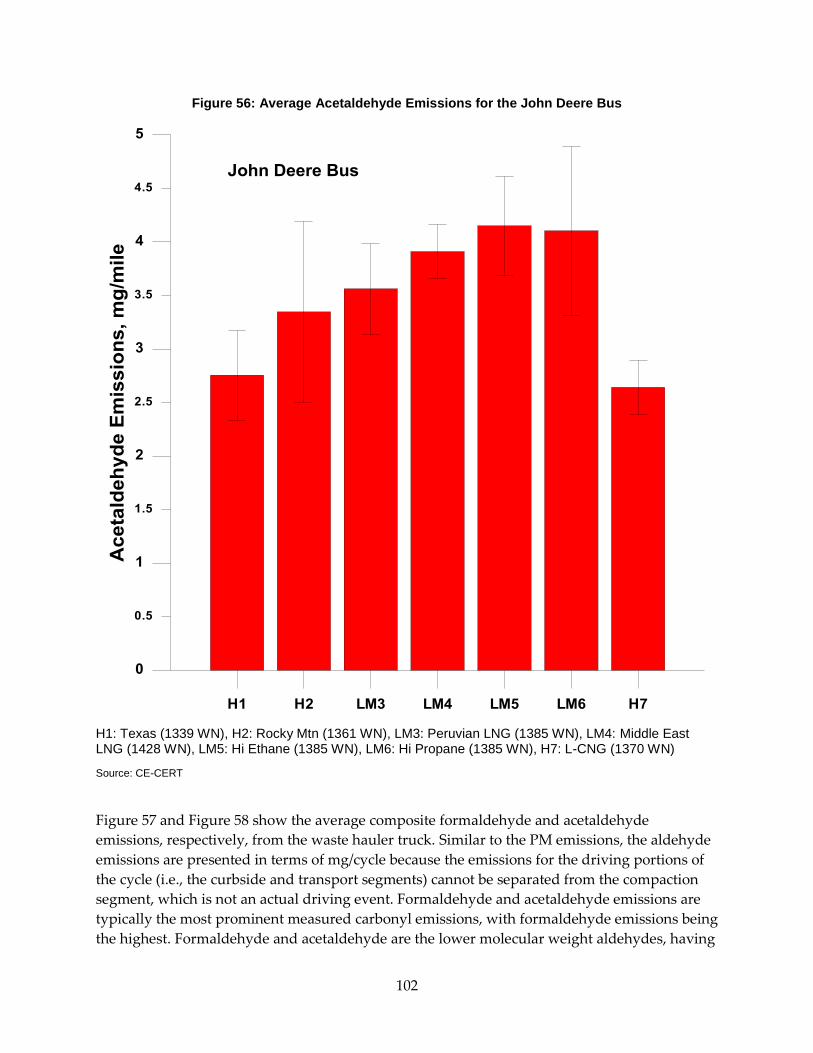
102

Figure 56: Average Acetaldehyde Emissions for the John Deere Bus


Source: CE-CERT

Figure 57 and Figure 58 show the average composite formaldehyde and acetaldehyde

emissions, respectively, from the waste hauler truck. Similar to the PM emissions, the aldehyde

emissions are presented in terms of mg/cycle because the emissions for the driving portions of

the cycle (i.e., the curbside and transport segments) cannot be separated from the compaction

segment, which is not an actual driving event. Formaldehyde and acetaldehyde emissions are

typically the most prominent measured carbonyl emissions, with formaldehyde emissions being

the highest. Formaldehyde and acetaldehyde are the lower molecular weight aldehydes, having

103

one and two carbons, respectively. Our results are consistent with previous studies showing

that the dominant carbonyl emissions from CNG vehicles come from the lowest molecular

weight compounds (Thiruvengadam, A. et al. 2011, Kado, N. et al. 2008, Okomoto, R. et al. 2006,

Durbin et al. 2014). Formaldehyde emissions do not show any statistically significant fuel

trends, with the exception of LM5 that shows a 54.7 percent decrease in formaldehyde

emissions compared to H1 at a statistically significant level. Acetaldehyde emissions are at or

below the background levels for most of the test fuels. Specifically, for all the test fuels with the

exception of H7, the emissions results are either negative or have error bars that extent below

zero. Acetaldehyde emissions show a marginally statistically significant increase of 313 percent

for H7 relative to H1. The legacy refuse hauler tested in Phase 1 showed higher levels of

formaldehyde and acetaldehyde compared to the refuse hauler in this study, with these two

being the dominant aldehydes in the tailpipe (Durbin et al. 2014). The legacy vehicle exhibited

strong trends for both aldehydes over the RTC, with the high methane fuels showing increased

formaldehyde and acetaldehyde emissions compared to the low methane fuels.

Figure 57: Average Formaldehyde Emissions for Waste Hauler


Source: CE-CERT

104

Figure 58: Average Acetaldehyde Emissions for Waste Hauler Truck


Source: CE-CERT

Figure 59 shows the formaldehyde and acetaldehyde emissions for the Cummins Westport ISL

G (A) truck and Cummins Westport ISX12 G (B) truck over the Near Dock duty cycle and the

Local Haul duty cycle, respectively. Formaldehyde and acetaldehyde emissions for these two

vehicles were collected cumulatively over the entire test cycles, without separating the

individual phases. Similar to the John Deere engine and the waste hauler truck, formaldehyde is

the predominant aldehyde in the tailpipe for both Cummins engines followed by acetaldehyde,

with the Cummins Westport ISX12 G engines showing higher aldehyde concentrations than the

Cummins Westport ISL G engine. For the Cummins Westport ISL G engine, formaldehyde

emissions show a declining trend for the low methane fuels and follow similar patterns with the

THC emissions. However, there are no statistically significant differences between the test fuels

105

for either the formaldehyde or the acetaldehyde emissions over the Near Dock duty cycle. For

the Cummins Westport ISX12 G truck, formaldehyde emissions show a marginally statistically

significant decrease of 41.6% for LM5 compared to H7, whereas acetaldehyde emissions show

statistically significant decreases of 61.6% and 67.8%, respectively, for LM5 compared to H1 and

H7. Formaldehyde and acetaldehyde emissions are also in agreement with THC emissions for

this engine, but not with NMHC emissions.

Figure 59: Formaldehyde and Acetaldehyde Emissions for the Cummins Westport ISL G (A) and Cummins Westport ISX12 G (B) Class 8 Trucks Over the Near Dock Cycle and the Local Haul Duty

Cycle


Source: CE-CERT

106

3.12 Nitrous Oxide Emissions

Nitrous oxide (N2O) is both a toxic pollutant and a greenhouse gas. Although aftertreatment

systems produce limited N2O, it is included in recent greenhouse gas regulations, which count

N2O as CO2 equivalents. N2O counts as a CO2 equivalent because, according to the Fifth

Assessment Report (AR5), N2O has a lifetime of approximately 121 years in the atmosphere and

a Global Warming Potential (GWP) of 265 based on a 100 year time horizon (265 times more

powerful than CO2 on heat trapping effects) (Myhre, G. et al. 2013). Besides, N2O is the major

source of NOx in the stratosphere; therefore, an important natural regulator of stratospheric

ozone.

Figure 60 shows the N2O emissions for the John Deere school bus over the CBD test cycle. For

the lean burn John Deere engine, N2O emissions trend higher for the low methane fuels, i.e.,

LM3, LM4, LM5, and LM6, compared to the high methane fuels of H1, H2, and H7. Emissions of

N2O show marginally statistically significant increases of 40 percent, 38 percent, 79 percent, and

45 percent for LM3, LM4, LM5, and LM6, respectively, compared to H1. Compared to H2, the

increases in N2O emissions are on the order of 144 percent, 140 percent, 211 percent, and 152

percent for LM3, LM4, LM5, and LM6, respectively, at a statistically significant level; however,

compared to H7 the increases in N2O emissions are on the order of 49 percent, 47 percent, 91

percent, and 55 percent for LM3, LM4, LM5, and LM6, respectively, at a statistically and

marginally statistically significant level.

107

Figure 60: N2O Emissions for the John Deere Bus


Source: CE-CERT

Figure 61 shows the composite N2O emissions for the waste hauler over the RTC. N2O

emissions ranged from 0.39 g/cycle to 1.27 g/cycle. Low methane fuels result in higher emissions

of N2O compared to the high methane fuels. The fuels LM3, LM5, and LM6 show statistically

significant increases in N2O emissions of 134.7 percent, 152.5 percent, and 107 percent and 200

percent, 223 percent, and 165 percent, respectively, compared to H1 and H7. N2O emissions

corroborate with NH3 emissions and show an inverse relation to NOx emissions for the

transport and curbside segments, as shown in Figure 8 (a-b).

108

Figure 61: N2O Emissions for the Waste Hauler over the RTC

H1-Texas (1339 WN), LM3Peruvian LNG (1385 WN), LM5-Hi Ethane (1385 WN), LM6-Hi Propane (1385 WN), H7 L-CNG (1370 WN)

Source: CE-CERT

Figure 62 shows the N2O emissions for the Cummins Westport ISL G (A) truck and the

Cummins Westport ISX12 G (B) truck over the Near Dock duty cycle and the Local Haul duty

cycle, respectively. In contracts to the NH3 emissions, the Cummins Westport ISL G truck

showed higher N2O emissions compared to the Cummins Westport ISX12 G truck. Analogous

to the John Deere bus and the waste hauler, both trucks show higher N2O emissions for the low

methane fuels. However, the differences in N2O emissions between the test fuels are not

statistically significant for either of the test vehicles.

Overall, our results show that selectivity towards N2O emissions is highly dependent on fuel

composition. All vehicles show a systematic increase in N2O emissions with the low methane

fuels, independent the engine technology and aftertreatment control. N2O forms as an

intermediate during the catalytic reduction of nitric oxide (NO) to molecular nitrogen (N2). At

high temperatures, NO is reduced to N2; however, at lower temperatures, N2O is an

intermediate product. Some of the reactions involve, which take place between species adsorb

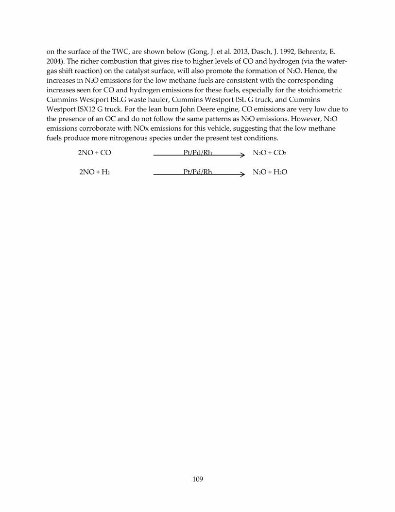
109

on the surface of the TWC, are shown below (Gong, J. et al. 2013, Dasch, J. 1992, Behrentz, E.

2004). The richer combustion that gives rise to higher levels of CO and hydrogen (via the water-

gas shift reaction) on the catalyst surface, will also promote the formation of N2O. Hence, the

increases in N2O emissions for the low methane fuels are consistent with the corresponding

increases seen for CO and hydrogen emissions for these fuels, especially for the stoichiometric

Cummins Westport ISLG waste hauler, Cummins Westport ISL G truck, and Cummins

Westport ISX12 G truck. For the lean burn John Deere engine, CO emissions are very low due to

the presence of an OC and do not follow the same patterns as N2O emissions. However, N2O

emissions corroborate with NOx emissions for this vehicle, suggesting that the low methane

fuels produce more nitrogenous species under the present test conditions.

2NO + CO

Pt/Pd/Rh

N2O + CO2

2NO + H2 Pt/Pd/Rh

N2O + H2O

110

Figure 62: N2O Emissions for the Cummins Westport ISL G (A) and Cummins Westport ISX12 G (B) Class 8 Trucks Over the Near Dock cycle and the Local Haul Duty


Source: CE-CERT

111

CHAPTER 4: Summary

As the demand for NG in California and the production of NG throughout the United States.

both expand, there is potential for a wider range of NG compositions to be used in NGVs. It is

important to evaluate whether changing NG composition will have adverse impacts on the

emissions or performance of NGVs. The current study addressed this issue. These results may

also be used in CARB’s ongoing process to amend the California NG fuel standards for motor

vehicles.

In this study, three to seven blends of natural gas with different fuel compositions were tested.

The fuels represent a range of compositions from fuels with high levels of methane and

correspondingly lower energy contents and Wobbe numbers to fuels with higher levels of

heavier hydrocarbons and correspondingly higher energy contents and Wobbe numbers.

Emission testing was performed on a school bus (with a 2005 lean-burn combustion spark

ignited engine and an oxidation catalyst), a waste hauler (with a 2011 stoichiometric spark

ignited engine with cooled EGR and TWC) and two Class 8 trucks (one truck with a 2012

stoichiometric spark ignited engine with cooled EGR and TWC and one truck with a 2013

stoichiometric spark ignited engine with cooled EGR and TWC) on CE-CERT’s heavy-duty

chassis dynamometer. The John Deere school bus was tested over the CBD test cycle, the waste

hauler was tested over the Refuse Truck cycle, while the Cummins Westport trucks were tested

over the Near Dock duty cycle and the Local Haul duty cycle, respectively. The results of the

test program show that fuel composition, engine operating conditions, and driving cycles had

effects on the formation of exhaust emissions for all three vehicles. Consistent fuel effects were

not seen for most of the pollutants for the newest technology vehicles with the stoichiometric

engine with a TWC, however.

The results of this study are summarized below. Results are generally statistically significant,

except as noted.

4.1 2005 John Deere School Bus

John Deere school bus emissions were evaluated over the Central Business District cycle on

seven of the test fuels. Overall, the lean-burn John Deere engine show the strongest fuel effects

for most of the pollutants compared to the stoichiometric Cummins trucks. Most pollutants

show some fuel effects over the CBD cycle. The low methane fuels show higher NOx, NMHC,

formaldehyde and acetaldehyde emissions, but lower THC and CH4 emissions. Fuel

economy/consumption on a volumetric basis shows increases for the low methane fuels with

higher energy contents. Fuel economy/consumption on an energy equivalent basis and carbon

dioxide emissions does not show strong trends. CO emissions are close to the tunnel

background levels and showed practically no fuel effects, while both increases and decreases

are seen for the PM mass emissions. Particle number show similar fuel trends over the three

cycle segments, but the fuels showing lower particle numbers include some high methane fuels

(i.e., H2) and some low methane fuels (i.e., LM3 and LM4). Ammonia emissions show some fuel

112

differences, but no consistent fuel trends over the CBD cycle. Additionally, ammonia emissions

are found at substantially lower levels than the stoichiometric Cummins engines.

4.2 2011 Cummins Westport ISL G Waste Hauler

The Cummins Westport ISL G waste hauler was tested on the Refuse Truck cycle on test fuels

H1, H7, LM3, LM5, and LM6. THC, NMHC, CH4, NOx, formaldehyde, and acetaldehyde

emissions for the Westport ISL-G waste hauler are considerably lower than these emissions

from previous studies of lean burn technology engines. The Cummins Westport ISL-G waste

hauler does; however, show higher CO and NH3 emissions compared to older lean burn

engines. The results show reductions in NOx emissions for the low methane fuels for the

Transport and Curbside cycles, which could be due to richer combustion with these fuels. NOx

emissions for the compaction cycle are very low. CO and NH3 emissions, on the other hand,

showed a trend of higher emissions for the low methane fuels, i.e., LM3, LM5, and LM6. THC

and CH4 emissions do not show any consistent fuel trends, while NMHC emissions show a

trend of higher emissions for the fuels containing higher levels of NMHCs (i.e., ethane, propane,

and butane). Fuel economy/consumption on a volumetric basis shows some differences

between the various test fuels, with LM3, LM5, and LM6, with low methane fuels showing

higher fuel economy on a volumetric basis compared to H1 and H7. Fuel

economy/consumption on an energy equivalent basis and CO2 emissions does not show

significant trends, except for some CO2 reductions for H7 compared to LM3, LM5, and LM6 for

the compaction cycle. PM mass and acetaldehyde emissions are very low for refuse truck on an

absolute level, are at the same levels as the tunnel background, and do not show statistically

significant differences between test fuels. PN emissions and formaldehyde emissions do not

show strong fuel trends for the different RTC segments. The particle size distributions show

bimodal distributions, with a majority of the particles in the nucleation mode with particle

diameters centered from 9 to 11 nm size range. N2O emissions show significant fuel effects, with

the low methane fuels resulting in higher emissions of N2O compared to high methane fuels.

4.3 2012 Cummins Westport ISL G Truck

The Cummins Westport ISL G truck was tested on the Near Dock duty cycle, which is a

segment of the drayage truck port cycle. Testing was conducting for only three of the main test

fuels, namely, H1, LM5, and LM6. Low methane fuels show lower THC and CH4 emissions. For

the NMHC emissions, there are some, but not consistent, increases with low methane fuels. The

low methane fuels show lower NOx emissions, while CO and NH3 emissions show increases

with the low methane fuels. Low methane fuels with higher energy contents show higher fuel

economy on a volumetric basis. One of the low methane fuels shows higher PM mass emissions,

while formaldehyde, acetaldehyde, and CO2 emissions do not show any significant fuel trends.

Particle size distributions show a bimodal particle size profile, with the accumulation mode

being the prevalent particles.

4.4 2013 Cummins Westport ISX12 G

The truck with a 2013 Cummins Westport ISX12 G was tested over the Local Haul duty cycle,

and was the newest technology tested during this program. In general, most of the gaseous

113

emissions for this engine are found at higher concentrations when compared to the Cummins

ISL G engines. NMHC, CO, and NH3 emissions are higher for the low methane fuels, while

NOx, THC, and CH4 emissions are lower for some low methane fuels. Volumetric fuel economy

and energy equivalent fuel economy are higher for the low methane fuels. CO2, PM mass,

formaldehyde and acetaldehyde emissions do not show strong trends between the test fuels.

The particle size distributions present a decidedly bimodal distribution and show a nucleation

peak around 10 nm. The accumulation mode particles range from 60 to 70 nm size range.

4.5 General

The results show that fuel composition, engine operating conditions, and driving cycle have

effects on the formation of exhaust emissions from all test vehicles. In general, low methane

fuels show higher NOx and NMHC emissions and improved fuel economy on a volumetric

basis, but lower THC and CH4 emissions. While these phenomena are particularly strong for the

older lean-burn John Deere engine, the newer stoichiometric Cummins engines also showed

relatively strong trends. For the gaseous toxic pollutants, such as formaldehyde and

acetaldehyde, the lean-burn technology bus shows the most consistent trends with the low

methane fuels showing higher emission levels of formaldehyde and acetaldehyde compared to

the high methane fuels. The stoichiometric Cummins vehicles with TWC systems show

significantly higher NH3 emissions than the lean-burn engine with the OC. For NH3 emissions,

the fuel effect is particularly strong with the low methane fuels showing higher NH3 emissions

than the high methane fuels. The trends for PM mass and particle number emissions are not as

consistent. Particle size distributions for all test vehicles show bimodal distributions with the

accumulation mode particles dominating the particle size distribution profile for most of the

test vehicles.

114

CHAPTER 5: Conclusions and Recommendations

As the demand for NG in California and the production of NG throughout the United States

both expand, there is potential for a wider range of natural gas compositions to be used in

NGVs. It is important to evaluate whether changing compositions of NG will have adverse

impacts on the emissions or performance of NGVs. The current study was designed to address

these issues. These results may also be used in CARB’s ongoing process to amend the California

NG fuel standards for motor vehicles.

In this study, three to seven blends of natural gas with different fuel compositions were tested.

The fuels represent a range of compositions from fuels with high levels of methane and

correspondingly lower energy contents and Wobbe numbers to fuels with higher levels of

heavier hydrocarbons and correspondingly higher energy contents and Wobbe numbers.

Emission testing was performed on one school bus (a bus with a 2005 lean-burn combustion

spark ignited engine and an OC), on a waste hauler with a 2011 stoichiometric spark ignited

engine and a TWC, and on two Class 8 trucks with 2012 and 2013 stoichiometric spark ignited

engines and a TWC, respectively, on CE-CERT’s heavy-duty chassis dynamometer.

The results show that fuel composition, engine operating conditions, and driving cycle have

effects on the formation of exhaust emissions from all test vehicles. The older vehicle shows

trends that are generally consistent with those of previous studies. Low methane fuels show

higher NOx and NMHC emissions and higher fuel economy on a volumetric basis but lower

emissions of THC and CH4. For the gaseous toxic pollutants, such as formaldehyde and

acetaldehyde, the lean-burn technology bus shows the most consistent trends with the low

methane fuels showing higher emission levels of formaldehyde and acetaldehyde compared to

high methane fuels. The stoichiometric Cummins vehicles with TWC systems show

significantly higher NH3 emissions than the lean-burn engine with the OC. For NH3 emissions,

the fuel effect is particularly strong with the low methane fuels showing higher NH3 emissions

than the high methane fuels. The trends for PM mass and particle number emissions are not as

consistent. Particle size distributions for all test vehicles show bimodal distributions with the

accumulation mode particles dominating the particle size distribution profile for most of the

test vehicles.

The results suggest that natural gas fuel composition can have an impact on emissions for older

technology heavy-duty vehicles, even for fuels within pipeline specifications, albeit at the

extreme ranges of what might be found in the pipeline. Control of natural gas specification is

still needed for older technology heavy-duty NGVs. Newer heavy-duty natural gas engines can

run on a wider range of NG fuels with varying composition, consistent with the Phase 1 results

of this program, and that this holds true for a wider range of applications, such as waste haulers

and port trucks.

115

GLOSSARY

Term Definition

ARB Air Resources Board

bhp brake horse power

bhp-hr brake horse power - hour

CAI California Analytical Instruments

CARB California Air Resources Board

CE-CERT College of Engineering-Center for Environmental Research and

Technology (University of California, Riverside)

CEC California Energy Commission

CBD Central Business District

CFR Code of Federal Regulations

CH4 Methane

CNG compressed natural gas

CO carbon monoxide

CO2 carbon dioxide

CPC condensation particle counter

DMA Differential Mobility Analyzer

DNPH 2,4-Dinitrophenylhydrazine

Dp particle diameter

DPF diesel particle filter

ECM engine control module

EEPS Engine Exhaust Particle Sizer

EGR exhaust gas recirculation

EIA Energy Information Administration

FID flame ionization detector

GGE gasoline gallon equivalent

g/mi grams per mile

HDV heavy-duty vehicle

HHV higher heating value

HPLC High Performance Liquid Chromatography

km kilometer

km/hr kilometers per hour

lbs. pounds

L-CNG CNG blend produced from an LNG fuel tank

LNG liquefied natural gas

MEL CE-CERT’s Mobile Emissions Laboratory

MN methane number

mpg miles per gallon

m/s2 meters per second squared

NDIR non-dispersive infrared detector

116

NG natural gas

NGL natural gas liquid

NGV natural gas vehicle

NH3 ammonia

nm nanometer

NMHC nonmethane hydrocarbons

NOx nitrogen oxides

OC Oxidation Catalyst

PAHs polycyclic aromatic hydrocarbons

PM particulate matter

PN particle number

SCAQMD South Coast Air Quality Management District

SOF soluble organic fraction

tcf trillion cubic feet

TDL tunable diode laser

THC total hydrocarbons

TWC Three-Way Catalyst

UCR University of California, Riverside

WN Wobbe number - higher heating value divided by the square root of

the specific gravity with respect to air

WVU West Virginia University

117

REFERENCES

Bach C. Challenges and Potential of Advanced Methane Gas Vehicles. In: SATW Congress,

August. 2008.

Behrentz E, Ling R, Rieger P, Winer AM. Measurements of nitrous oxides emissions from light-

duty motor vehicles: a pilot study. Atmospheric Environment 2004, 38, 4291-4303.

Bielaczyc P, Szczotka A, Swiatek A, Woodburn J. A comparison of ammonia emissions factors

from light-duty vehicles operating on gasoline, liquefied petroleum gas (PG) and

compressed natural gas (CNG). SAE Technical Paper 2012, 2012-01-1095.

Burcat A, Scheller K, Lifshitz A. Shock-tube investigation of comparative ignition delay times

for C1-C5 alkanes. Combustion and Flame. 1971;16(1):29–33.

California Air Resources Board, http://www.arb.ca.gov/fuels/altfuels/cng/cng.htm.

Chiu JP, Taylor JD, Tai C, Reppert T, Christensen L. US 2010 Emissions Capable Camless

Heavy-Duty On-Highway Natural Gas Engine. SAE Technical Paper 2007-01-1930, 2007.

Dasch JM. Nitrous oxides from vehicles. Journal of the Air & Waste Management Association

1992, 42, 63-67.

Durbin T, Karavalakis G, Johnson K, Miller J, Hajbabaei, M. Evaluation of the Performance and

Air Pollutant Emissions of Vehicles Operating on Various Natural Gas Blends – Heavy-

Duty Vehicle Testing. Final Report submitted to California Energy Commission (CEC),

2014.

Einewall P, Tunestål P, Johansson B. Lean Burn Natural Gas Operation vs. Stoichiometric

Operation with EGR and a Three Way Catalyst. SAE Technical Paper. 2005;(2005-01-

0250).

Elder ST, Jones K, Taine RR. Effects of Varying fuel Composition on the Performance of CNG

and LPG Fuelled Vehicles. In: Professional Engineers of New Zealand Transcripts. Vol.

12, No. 3/EMCh, November. 1985.

Energy Information Administration, 2013, AEO2013 Early Release Overview [Internet].

Available from: http://www.eia.gov/forecasts/aeo/er/index.cfm

Energy Information Administration, 2012, Annual Energy Outlook 2012 [Internet]. Available

from: http://www.eia.gov/forecasts/aeo/MT_naturalgas.cfm

Feist MD. Fuel Composition Testing using DDC Series 50G Natural Gas Engines. Final report

prepared by Southwest Research Institute for the Southern California Gas Company,

Report No. 11657, August 2006.

Feist MD. Fuel Composition Testing using Cummins, John Deere, and Detroit Diesel Natural

Gas Engines. Final report prepared by Southwest Research Institute for the Southern

California Gas Company, Report No. 03.13721, April 2009.

http://digitallibrary.sae.org/content/2007-01-1930

http://digitallibrary.sae.org/content/2007-01-1930

118

Fiest M., Landau M, Harte E. The effect of Fuel Composition on Performance and Emissions of a

Variety of Natural Gas Engines. SAE Technical Paper. 2010;(2010-01-1476).

Fontaras G, Martini G, Manfredi U, Marotta A, Krasenbrink A, Maffioletti F, et al. Assessment

of On-road Emissions of Four Euro V Diesel and CNG Waste Collection Trucks for

Supporting Air-quality Improvement Initiatives in the City of Milan. Science of the Total

Environment. 2012;426:65–72.

Gandhi HS SM. Ammonia Formation in the Catalytic Reduction of Nitric Oxide. III. The Role of

Water Gas Shift, Reduction by Hydrocarbons, and Steam Reforming. Ind. Eng. Chem.,

Prod. Res. Dev. 1974;13:80–5.

Gong J, Rutland C. Three way catalyst modeling with ammonia and nitrous oxide kinetics for a

lean burn spark ignition direct injection (SIDI) gasoline engine. SAE Technical Paper

2013, 2013-01-1572.

Gutierrez JH, Saldivar AR, Mora JR. LNG Research Study – Phase 1. Testing of a Natural Gas

Compressor Engine. Report by the Southern California gas Company, October 2003.;

2003.

Gutierrez J, Hamze F, Mak C. LNG Research Study [Internet]. April 2006.; Report by the

Southern California gas Company; 2006. Available from:

http://www.socalgas.com/documents/business/gasquality/Richburn_engine_report.pdf

Hajbabaei M., Karavalakis G., Kent C. Johnson, Linda Lee, Thomas D. Durbin. Impact of natural

gas fuel composition on criteria, toxic, and particle emissions from transit buses

equipped with lean burn and stoichiometric engines. Energy 2013, 62, 425-434.

Hesterberg TW, Lapin CA, Bunn WB. A Comparison of Emissions from Vehicles Fueled with

Diesel or Compressed Natural Gas. Environmental Science & Technology. 2008;42:6437–

45.

Holmen B, Ayala A. Ultrafine PM Emissions from Natural Gas, Oxidation Catalyst Diesel and

Particle Trap Diesel Heavy-duty Transit Buses. Environmental Science & Technology.

2002;36:5041–50.

Huai T, Durbin T, Miller J, Pisano J, Sauer C, Rhee S, et al. Investigation of NH3 Emissions from

New Technology Vehicles as a Function of Vehicle Operating Conditions.

Environmental Science & Technology. 2003; 37:4841–7.

Jayaratne E, Ristovski Z, Meyer N, Morawska L. Particle and Gaseous Emissions from

Compressed Natural Gas and Ultralow Sulphur Diesel-fuelled Buses at Four Steady

Engine Loads. Science of the Total Environment. 2009;407:2845–52.

Jayaratne E, Meyer N, Ristovski Z, Morawska L. Volatile Properties of Particles Emitted by

Compressed Natural Gas and Diesel Buses during Steady-State and Transient Driving

Modes. Environmental Science & Technology. 2012;46:196–203.

119

Kado N, Okomoto RA, Kuzmicky P, Kobayashi R, Ayala A. Emissions of Toxic pollutants from

Compressed Natural Gas and Low Sulfur Diesel-fueled Heavy-duty Transit Buses

Tested over Multiple Driving Cycles. Environmental Science & Technology.

2008;29:7638–49.

Karavalakis G., Hajbabaei M., Durbin T.D., Johnson K.C., Zheng Z., Miller W.J. The effect of

natural gas composition on the regulated emissions, gaseous toxic pollutants, and

ultrafine particle number emissions from a refuse hauler vehicle. Energy 2013, 50, 280-

291.

Khalek A, Kittelson DB, Graskow BR, Wei Q, Diesel exhaust particle size: Measurement issues

and trends. SAE Technical Paper 1998, 980525.

Lee Y-J, Kim G-C. Effect of Gas Composition on NGV Performance. In: Seoul 2000 FISITA

World Automotive Congress, June, Seoul, Korea. 2000.

Ma F, Wang Y, Liu H, Li Y, Wang J, Zhao S. Experimental Study on Thermal Efficiency and

Emission Characteristics of a Lean Burn Hydrogen Enriched Natural Gas Engine.

International Journal of Hydrogen Energy. 2007;32:5067–75.

Malenshek, M. and Olsen D. Methane Number Testing of Alternative Gaseous Fuels. Fuel.

2009;88:650–6.

Matthews R, Chiu J, Hilden D. CNG Compositions in Texas and the Effects of Composition on

Emissions, Fuel Economy, and Drivability of NGVs. SAE Technical Paper. 1996;(962097).

McTaggart GP, Rogak SN, Munshi SR, Hill PG, Bushe W. The Influence of Fuel Composition on

a Heavy-duty, Natural-gas Direct-injection Engine. Fuel. 2010;89:752–9.

Mejia-Centeno I, Martinez-Hernadez A, Fuentes GA. Effect of low-sulfur fuels upon NH3 and

N2O emission during operation of commercial three-way catalytic converters. Topics in

Catalysis 2007, 42-43, 381-385.

Min BH, Chung JT, Kim HY, Park S. Effects of Gas Composition on the Performance and

Emissions of Compressed Natural Gas Engines. KSME International Journal.

2002;16:219–26.

Myhre, G., D. Shindell, F.-M. Bréon, W. Collins, J. Fuglestvedt, J. Huang, D. Koch, J.-F.

Lamarque, D. Lee, B. Mendoza, T. Nakajima, A. Robock, G. Stephens, T. Takemura and

H. Zhang, 2013: Anthropogenic and Natural Radiative Forcing. In: Climate Change 2013: The

Physical Science Basis. Contribution of Working Group I to the Fifth Assessment Report

of the Intergovernmental Panel on Climate Change [Stocker, T.F., D. Qin, G.-K. Plattner,

M. Tignor, S.K. Allen, J. Boschung, A. Nauels, Y. Xia, V. Bex and P.M. Midgley (eds.)].

Cambridge University Press, Cambridge, United Kingdom and New York, NY, USA.

Naber JD, Siebers DL, Caton JA, Westbrook CK, Di Julio SS. Natural Gas Autoignition under

Diesel Conditions: Experiments and Kinetic Modeling. SAE Technical Paper.

1994;(942034).

120

NGC+ Interchangeability Work Group. White Paper on Natural Gas Interchangeability and

Non-Combustion End Use. 2005.

NGC+ Liquid Hydrocarbon Drop Out Task Group. White Paper on Liquid Hydrocarbon Drop

Out in Natural Gas Infrastructure. 2005.

Okomoto RA, Kado N, Kuzmicky P, Ayala A. Unregulated Emissions from Compressed

Natural Gas (CNG) Transit Buses Configured with and without Oxidation Catalyst.

Environmental Science & Technology. 2006;40:332–41.

Siegl, W.O.; Richert, J.F.O.; Jensen, T.E.; Schuetzle, D.; Swarin, S.J.; Loo, J.F.; Prostak, A.; Nagy,

D.; and Schlenker, A.M. “Improved Emissions Speciation Methodology for Phase II of

the Auto/Oil Air Quality Improvement Research Program – Hydrocarbons and

Oxygenates”, SAE Technical Paper 930142. Warrendale, PA: Society of Automotive

Engineers, 1993.

The International Council on Clean Transportation, 2009, CNG Bus Emissions Roadmap: from

Euro III to Euro VI.

http://www.theicct.org/sites/default/files/publications/CNGbuses_dec09.pdf.

Thiruvengadam A, Carder DK, Krishnamurthy M, Oshinuga A, Gautam M. Effect of an

Economical Oxidation Catalyst Formulation on Regulated and Unregulated Pollutants

from Natural Gas Fueled Heavy Duty Transit Buses. Transportation Research Part D.

2011;16:469–73.

Thiruvengadam A, Besch MC, Yoon S, Collins J, Kappanna H, Carder DK, Ayala A, Herner H,

Gautam M. Characterization of particulate matter emissions from a current technology

natural gas engine. Environ Sci Technol 2014, 48, 8235-8242.

Walkowicz K, Proc K, Wayne S, Nine R, Campbell K, Wiedemeier G. Chassis Dynamometer

Emission Measurements from Refuse Trucks using Dual-fuel Natural Gas Engines. SAE

Technical Paper. 2003;(2003-01-3366).

Wang WG, Clark NN, Lyons DW, Yang RM, Gautam M, Bata RM LJ. Emissions Comparisons

from Alternative Fuel Buses and Diesel Buses with Chassis Dynamometer.

Environmental Science & Technology. 1997;31:3132–7.

Yoon S, Hu S, Collins J, Herner J, Thiruvengadam A, Carder D, et al. Comparison of

Unregulated Emissions from CNG Buses with and without Aftertreatment Technologies.

In: 22nd CRC Real World Emissions Workshop. 2012.

Zarante PHB, Sodre JR. Evaluating Carbon Emission Reduction by Use of Natural Gas as

Engine Fuel. Journal of Natural Gas Science and Engineering. 2009;1:216–20.

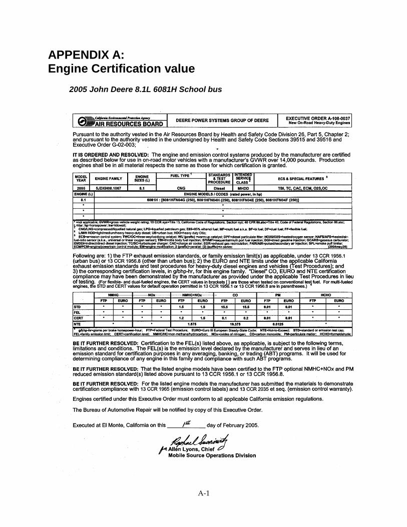
A-1

APPENDIX A: Engine Certification value

2005 John Deere 8.1L 6081H School bus

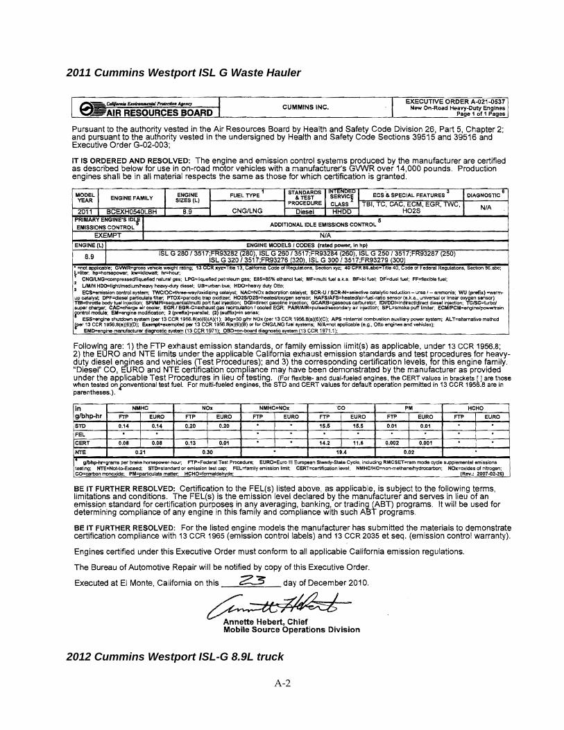
A-2

2011 Cummins Westport ISL G Waste Hauler

2012 Cummins Westport ISL-G 8.9L truck

A-4

2013 Cummins Westport ISX12G 11.9 L truck

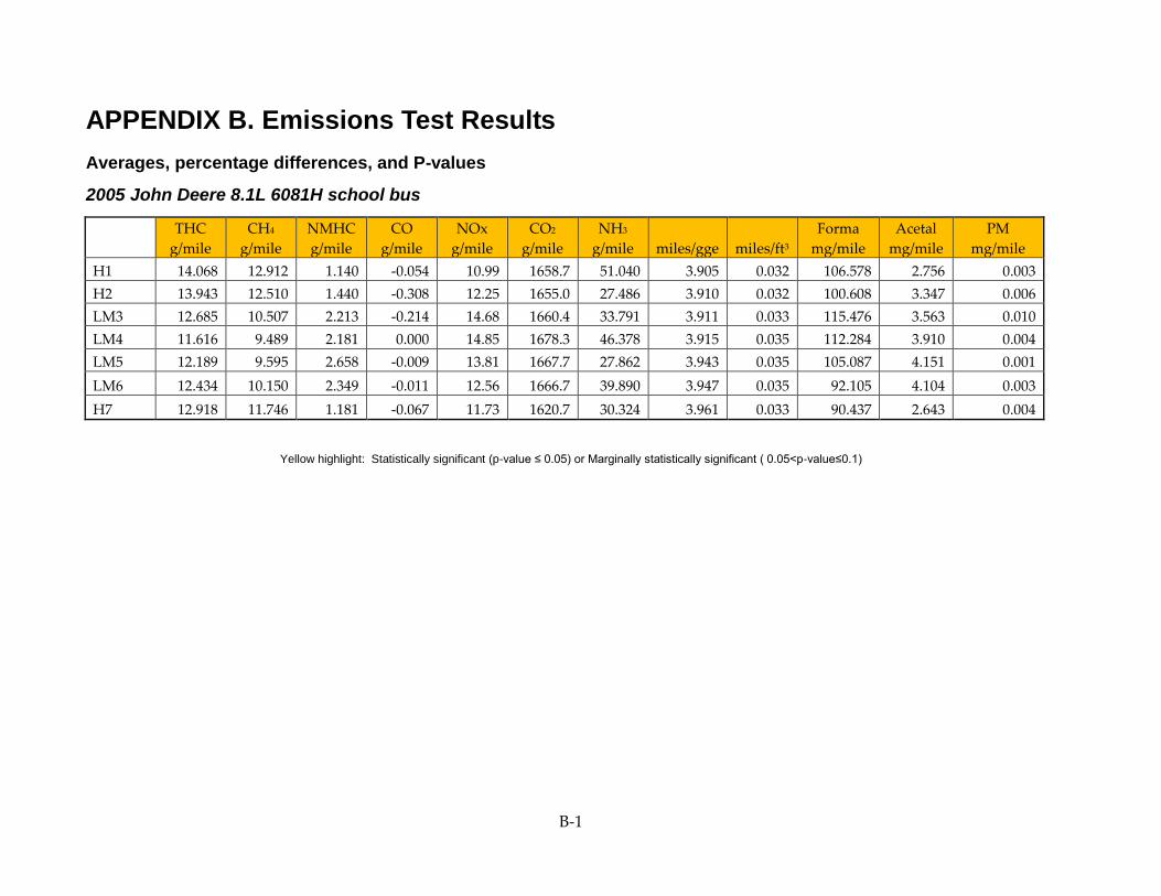
B-1

APPENDIX B. Emissions Test Results

Averages, percentage differences, and P-values

2005 John Deere 8.1L 6081H school bus

THC

g/mile

CH4

g/mile

NMHC

g/mile

CO

g/mile

NOx

g/mile

CO2

g/mile

NH3

g/mile miles/gge miles/ft3

Forma

mg/mile

Acetal

mg/mile

PM

mg/mile

H1 14.068 12.912 1.140 -0.054 10.99 1658.7 51.040 3.905 0.032 106.578 2.756 0.003

H2 13.943 12.510 1.440 -0.308 12.25 1655.0 27.486 3.910 0.032 100.608 3.347 0.006

LM3 12.685 10.507 2.213 -0.214 14.68 1660.4 33.791 3.911 0.033 115.476 3.563 0.010

LM4 11.616 9.489 2.181 0.000 14.85 1678.3 46.378 3.915 0.035 112.284 3.910 0.004

LM5 12.189 9.595 2.658 -0.009 13.81 1667.7 27.862 3.943 0.035 105.087 4.151 0.001

LM6 12.434 10.150 2.349 -0.011 12.56 1666.7 39.890 3.947 0.035 92.105 4.104 0.003

H7 12.918 11.746 1.181 -0.067 11.73 1620.7 30.324 3.961 0.033 90.437 2.643 0.004

Yellow highlight: Statistically significant (p-value ≤ 0.05) or Marginally statistically significant ( 0.05<p-value≤0.1)

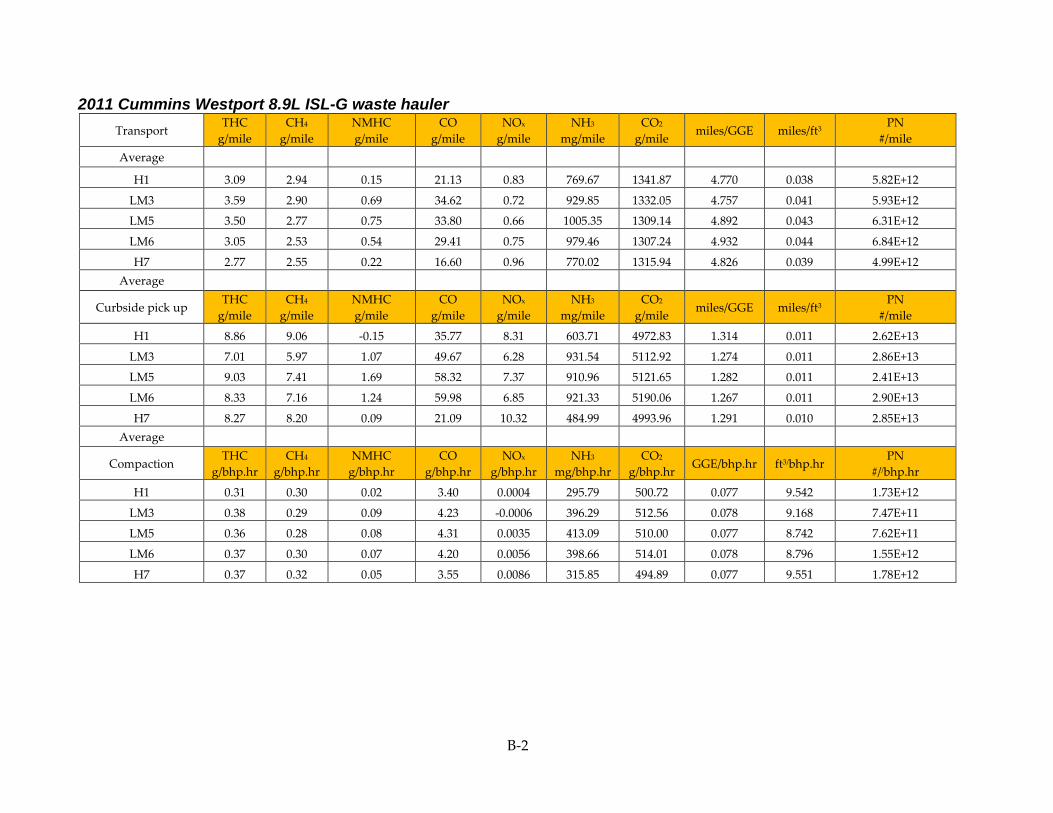
B-2

2011 Cummins Westport 8.9L ISL-G waste hauler

Transport THC

g/mile

CH4

g/mile

NMHC

g/mile

CO

g/mile

NOx

g/mile

NH3

mg/mile

CO2

g/mile miles/GGE miles/ft3

PN

#/mile

Average

H1 3.09 2.94 0.15 21.13 0.83 769.67 1341.87 4.770 0.038 5.82E+12

LM3 3.59 2.90 0.69 34.62 0.72 929.85 1332.05 4.757 0.041 5.93E+12

LM5 3.50 2.77 0.75 33.80 0.66 1005.35 1309.14 4.892 0.043 6.31E+12

LM6 3.05 2.53 0.54 29.41 0.75 979.46 1307.24 4.932 0.044 6.84E+12

H7 2.77 2.55 0.22 16.60 0.96 770.02 1315.94 4.826 0.039 4.99E+12

Average

Curbside pick up THC

g/mile

CH4

g/mile

NMHC

g/mile

CO

g/mile

NOx

g/mile

NH3

mg/mile

CO2

g/mile miles/GGE miles/ft3

PN

#/mile

H1 8.86 9.06 -0.15 35.77 8.31 603.71 4972.83 1.314 0.011 2.62E+13

LM3 7.01 5.97 1.07 49.67 6.28 931.54 5112.92 1.274 0.011 2.86E+13

LM5 9.03 7.41 1.69 58.32 7.37 910.96 5121.65 1.282 0.011 2.41E+13

LM6 8.33 7.16 1.24 59.98 6.85 921.33 5190.06 1.267 0.011 2.90E+13

H7 8.27 8.20 0.09 21.09 10.32 484.99 4993.96 1.291 0.010 2.85E+13

Average

Compaction THC

g/bhp.hr

CH4

g/bhp.hr

NMHC

g/bhp.hr

CO

g/bhp.hr

NOx

g/bhp.hr

NH3

mg/bhp.hr

CO2

g/bhp.hr GGE/bhp.hr ft3/bhp.hr

PN

#//bhp.hr

H1 0.31 0.30 0.02 3.40 0.0004 295.79 500.72 0.077 9.542 1.73E+12

LM3 0.38 0.29 0.09 4.23 -0.0006 396.29 512.56 0.078 9.168 7.47E+11

LM5 0.36 0.28 0.08 4.31 0.0035 413.09 510.00 0.077 8.742 7.62E+11

LM6 0.37 0.30 0.07 4.20 0.0056 398.66 514.01 0.078 8.796 1.55E+12

H7 0.37 0.32 0.05 3.55 0.0086 315.85 494.89 0.077 9.551 1.78E+12

B-3

2012 Cummins Westport 8.9L ISL-G truck

THC

g/mile

CH4

g/mile

NMHC

g/mile

CO

g/mile

NOx

g/mile

CO2

g/mile

NH3


Formal

mg/mile

Acetal

mg/mile

PM

mg/mile

H1 Total1 4.601 4.543 0.073 4.611 9.005 2122.59 575.674 3.079 0.025 12.643 0.733 0.0028

Phase 1 199.204 186.233 12.957 40.371 162.175 22855.37 335.433 0.282 0.002

Phase 2 13.137 12.788 0.379 1.514 28.312 3714.88 163.421 1.758 0.014

Phase 3 2.161 2.230 -0.056 4.746 5.495 1776.40 629.230 3.686 0.030

LM5 Total 3.658 3.379 0.328 9.735 7.088 2139.27 786.925 3.100 0.027 12.564 0.309 0.0044

Phase 1 134.386 107.503 27.690 3.834 163.472 21253.02 429.803 0.318 0.003

Phase 2 9.016 8.118 1.007 7.232 22.228 3751.17 503.434 1.772 0.016

Phase 3 1.935 1.950 0.021 10.084 3.921 1782.17 825.508 3.722 0.033

LM6 Total 3.880 3.979 -0.021 11.101 5.701 2117.68 676.097 3.130 0.028 5.199 -0.341 0.0027

Phase 1 167.856 160.653 9.728 40.163 165.727 24523.82 504.533 0.272 0.002

Phase 2 9.046 9.397 -0.163 5.831 20.805 3764.99 478.265 1.769 0.016

Phase 3 2.149 2.262 -0.066 11.564 2.736 1762.04 701.416 3.760 0.033

1 The individual phases are Phase 1 = creep phase, Phase 2 = a low speed transient phase, and Phase 3 = a short high-speed transient phase.

B-4

2013 Cummins Westport 11.9L ISX12G truck

THC

g/mile

CH4

g/mile

NMHC

g/mile

CO

g/mile

NOx

g/mile

CO2

g/mile

NH3


PM

mg/mile

Formal

mg/mile

Acetal

mg/mile

H1 Total2 1.969 1.924 0.050 10.046 0.507 2188.21 878.248 2.987 0.024 0.018 16.71 7.66

Phase 1 46.931 44.736 2.245 2.748 4.525 24123.85 676.144 0.276 0.002

Phase 2 20.628 19.636 1.013 13.921 2.163 4304.65 832.175 1.506 0.012

Phase 3 0.508 0.537 -0.025 9.802 0.376 1964.85 882.330 3.331 0.027

LM4 Total 1.919 1.765 0.176 14.211 0.514 2205.78 1131.954 3.000 0.027 0.02545 21.93 11.37

Phase 1 52.935 50.346 3.342 16.404 2.620 24078.69 429.650 0.279 0.003

Phase 2 17.084 15.136 2.122 31.076 1.472 4278.85 1526.259 1.536 0.014

Phase 3 0.626 0.620 0.016 13.456 0.401 1985.17 1125.560 3.336 0.030

LM5 Total 1.917 1.776 0.159 16.099 0.409 2157.66 1186.863 3.067 0.027 0.01948 11.93 2.945

Phase 1 49.032 45.508 3.987 12.550 4.548 29227.82 550.977 0.238 0.002

Phase 2 17.929 15.416 2.613 33.566 1.460 4398.62 1791.834 1.491 0.013

Phase 3 0.672 0.706 -0.022 14.884 0.324 1925.69 1146.363 3.440 0.030

H7 Total 2.281 2.294 0.001 10.439 0.512 2142.28 972.635 3.035 0.025 0.018 20.43 9.148

Phase 1 73.481 71.317 2.491 18.537 5.955 22936.17 326.990 0.286 0.002

Phase 2 23.072 22.067 1.090 21.669 2.182 4520.54 1619.363 1.454 0.012

Phase 3 0.570 0.661 -0.083 9.628 0.376 1903.36 929.983 3.420 0.028

2 The individual phases are Phase 1 = creep phase, Phase 2 = a low speed transient phase, and Phase 3 = a long high-speed transient phase.

C-1

APPENDIX C : Fuel Economy/Consumption Calculation

Fuel Economy Calculated on a Gasoline Gallon Energy Equivalent Basis

Note that the above equation is slightly modified from that given in the US EPA Code of Federal Regulations to account for the differences in the

energy content and other properties of the test gases

Fuel Economy Calculated Based on Volume of Natural Gas Consumed

mpge = miles per equivalent gallon of natural gas

mpgv = miles per cubic feet of natural gas fuel consumed

CWFHC/NG = carbon weight fraction based on the hydrocarbon constituents in the natural gas fuel

CWFNG = carbon weight fraction of the natural gas fuel

DNG = density of the natural gas fuel [grams/ft3 at 68°F (20°C) and 14.696 psi (760 mm Hg, or 101.325 kPa)]

= specific gravity of fuel x 28.316847 liters/ft3 x density of air (1.2047 g/l) [1, 2]

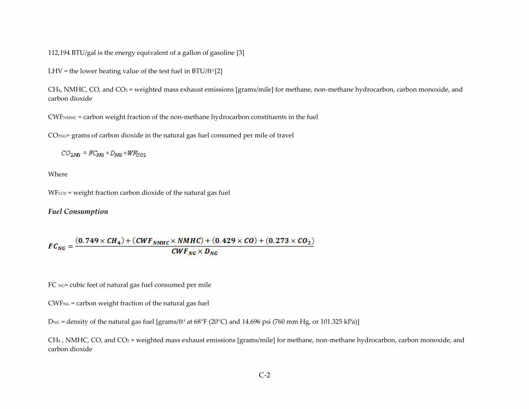
C-2

112,194 BTU/gal is the energy equivalent of a gallon of gasoline [3]

LHV = the lower heating value of the test fuel in BTU/ft3 [2]

CH4, NMHC, CO, and CO2 = weighted mass exhaust emissions [grams/mile] for methane, non-methane hydrocarbon, carbon monoxide, and

carbon dioxide

CWFNMHC = carbon weight fraction of the non-methane hydrocarbon constituents in the fuel

CO2NG= grams of carbon dioxide in the natural gas fuel consumed per mile of travel

Where

WFCO2 = weight fraction carbon dioxide of the natural gas fuel

Fuel Consumption

FC NG= cubic feet of natural gas fuel consumed per mile

CWFNG = carbon weight fraction of the natural gas fuel

DNG = density of the natural gas fuel [grams/ft3 at 68°F (20°C) and 14.696 psi (760 mm Hg, or 101.325 kPa)]

CH4 , NMHC, CO, and CO2 = weighted mass exhaust emissions [grams/mile] for methane, non-methane hydrocarbon, carbon monoxide, and

carbon dioxide

C-3

CWFNMHC = carbon weight fraction of the non-methane hydrocarbon constituents in the fuel

Gas Methane Ethane Propane i-Butane n-Butane i-Pentane n-

Pentane C6+ CO2 O2 N2 CWFHC/NG CWFNG CWFNMHC DNG LHV

H1 96.00 1.80 0.40 0.15 0.00 0.00 0.00 0.00 0.95 0.00 0.70 0.724 0.731 0.806 19.844 903.8

H2 94.50 3.50 0.60 0.30 0.00 0.00 0.00 0.00 0.75 0.00 0.35 0.735 0.740 0.805 20.151 926.6

LM3 88.30 10.50 0.00 0.00 0.00 0.00 0.00 0.00 0.00 0.00 1.20 0.743 0.743 0.799 20.840 960.3

LM4 89.30 6.80 2.60 1.30 0.00 0.00 0.00 0.00 0.00 0.00 0.00 0.762 0.762 0.809 21.570 1008.3

LM5 83.65 10.75 2.70 0.2 0.00 0.00 0.00 0.00 0.00 0.00 2.70 0.732 0.732 0.804 22.092 990.4

LM6 87.20 4.50 4.40 1.20 0.00 0.00 0.00 0.00 0.00 0.00 2.70 0.732 0.732 0.813 22.116 990.9

H7 98.44 1.23 0.25 0.08 0.00 0.00 0.00 0.00 0.00 0.00 0.00 0.750 0.750 0.805 19.25 911.0

* DNG = density of the natural gas fuel [grams/ft3 at 68°F (20°C) and 14.696 psi (760 mm Hg, or 101.325 kPa)]

** LHV = the lower heating value of the test fuel in BTU/ft3 at 68°F (20°C) and 14.696 psi (760 mm Hg, or 101.325 kPa)

Note: that the calculations in this appendix are based on a temperature of 68°F and a pressure of 14.696, as opposed to the 60°F and

14.73 psi used for the characterization of the gases in. This was to ensure that all the constants and values, such as WI, density and

heating value, used in these formulas were calculated based on the same temperature and pressure basis used in the Code of Federal

Regulations.

References

1. Environmental Protection Agency, National Vehicle and Fuel Emissions Laboratory (NVFEL) Emissions Analysis,

http://www.epa.gov/nvfel/testing/methods.htm

2. American Gas Association Report No.5, “Natural Gas Energy Measurement”, AGA 5 Calculation Spreadsheet – Imperial Units of

Measure, version 1.1, Feb 26, 2008

3. US Dept. of Energy, Argonne National Laboratory, GREET 1 2013, The Greenhouse Gases, Regulated Emissions, and Energy Use

in Transportation Model, http://greet.es.anl.gov/, 2013

4. Code of Federal Regulations, Part 600, Subpart B- Fuel Economy and Carbon-Related Exhaust Emission Test Procedures, 2012.

http://greet.es.anl.gov/

EVALUATION OF THE PERFORMANCE AND AIR POLLUTANT EMISSIONS ...€¦ · The evaluation of the...

Documents

Transcript of EVALUATION OF THE PERFORMANCE AND AIR POLLUTANT EMISSIONS ...€¦ · The evaluation of the...