Evaluation of Strength and Hydraulic Properties of Buried ...

University of Central Florida University of Central Florida

STARS STARS

Electronic Theses and Dissertations, 2004-2019

2015

Evaluation of Strength and Hydraulic Properties of Buried Pipe Evaluation of Strength and Hydraulic Properties of Buried Pipe

Systems Used for Stormwater Harvesting Systems Used for Stormwater Harvesting

Mario Samson Mena University of Central Florida

Part of the Civil Engineering Commons, Geotechnical Engineering Commons, and the Structural

Engineering Commons

Find similar works at: https://stars.library.ucf.edu/etd

University of Central Florida Libraries http://library.ucf.edu

This Masters Thesis (Open Access) is brought to you for free and open access by STARS. It has been accepted for

inclusion in Electronic Theses and Dissertations, 2004-2019 by an authorized administrator of STARS. For more

information, please contact [email protected].

STARS Citation STARS Citation Samson Mena, Mario, "Evaluation of Strength and Hydraulic Properties of Buried Pipe Systems Used for Stormwater Harvesting" (2015). Electronic Theses and Dissertations, 2004-2019. 1433. https://stars.library.ucf.edu/etd/1433

https://stars.library.ucf.edu/



https://stars.library.ucf.edu/etd

http://network.bepress.com/hgg/discipline/252?utm_source=stars.library.ucf.edu%2Fetd%2F1433&utm_medium=PDF&utm_campaign=PDFCoverPages




https://stars.library.ucf.edu/etd

http://library.ucf.edu/

mailto:[email protected]

https://stars.library.ucf.edu/etd/1433?utm_source=stars.library.ucf.edu%2Fetd%2F1433&utm_medium=PDF&utm_campaign=PDFCoverPages



EVALUATION OF STRENGTH AND HYDRAULIC PROPERTIES OF BURIED PIPE

SYSTEMS USED FOR STORMWATER HARVESTING

by

MARIO SAMSON

B.S. University of Central Florida, 2015

A thesis submitted in partial fulfillment of the requirements

for the degree of Master of Science

in the Department of Civil and Environmental Engineering

in the College of Engineering and Computer Science

at the University of Central Florida

Orlando, Florida

Spring Term

2015

ii

© 2015Mario R. Samson Mena

iii

ABSTRACT

Water scarcity has been identified as a global issue. Both water harvesting and an

efficient water piping system are some of the important factors to meet the water demand. In this

study, high-density polyethylene (HDPE) pipes used as an underground storage was evaluated

and a Microsoft EXCEL based model was developed, called PIPE-R Model. To study the

structural integrity of the pipes, laboratory and field testing were conducted. For the water

harvesting, UCF Stormwater Management Academy designed an EXCEL based model to

simulate the system’s performance to store and redistribute water for an average year.

The purpose of PIPE-R Model was to provide average yearly values such as groundwater

recharge, hydrologic efficiency and make up water needed in order to guide the user in the

design process. The PIPE-R Model consisted on evaluating specific pipe systems based on

properties selected by the user. Input variables such as system dimensions, soil type and reuse

water demand provided flexibility to the user while evaluating the system. Results of the study

showed that the PIPE-R Model might be an effective tool while designing these pipe systems. A

detailed example was shown to help visualize the process required to use the model. The PIPE-R

model allowed the user a wide range of possibilities and obtain important performance data that

will hopefully optimize the cost for its construction.

For the evaluation of the structural integrity of the pipe system, laboratory testing was

conducted in accordance with ASTM D2412 − 11 “Determination of External Loading

Characteristics of Plastic Pipe by Parallel-Plate Loading”. This method helps evaluate the

structural performance based on the pipe stiffness (PS) against the standard values stated by

AASHTO M252. The test procedure consisted on establishing load-deflection relationship of a

iv

single pipe under parallel plate loading. However, this research project involved the analysis of

bundled pipes of different sizes and levels. Thus, modifications were added to the formula in

order to evaluate multiple pipes by accounting the number of pipes in contact with the loading

plate. Laboratory results demonstrated that the pipes exceeded the minimum requirements stated

by AASHTO M252 and that strength is decreased as the number of levels increases.

In addition, field testing was conducted to study the behavior of bundle systems under

the effects of dead and live loads. Three different cover configuration were studied ranging from

18 inches to 43 inches of depth. Draw-wire sensors, a type of displacement sensors, were placed

inside buried housing structures to monitor deformation values experienced by the pipe bundles

during the test. Average deformations founds for the cover depths of 43 in, 30 in and 18 in were

0.07 in, 0.32 in and 0.64 in, respectively. Based on these results, the field testing revealed that a

minimum of 30 inches of cover is seemed to be appropriate if live loads are applicable.

v

ACKNOWLEDGMENTS

I would like to thank my committee members Dr. Gogo-Abite, Dr. Wang and Dr. Nam as

well as the students of the Stormwater Management Academy. Special thanks to Dr. Chopra for

providing me with this opportunity and encouraging me to achieve my goals. I would also like to

thank Antony for his help during this project.

I would also like to thank my family and friends for all their support and encouragement.

I would not have been able to accomplish this without the support of my dad, mom and

girlfriend. I would now like to thank Dr. Gogo-Abite and Dr. Hardin for being such a great

mentors throughout this project, I have learned skills that will help tremendously in and out of

the engineering profession.

vi

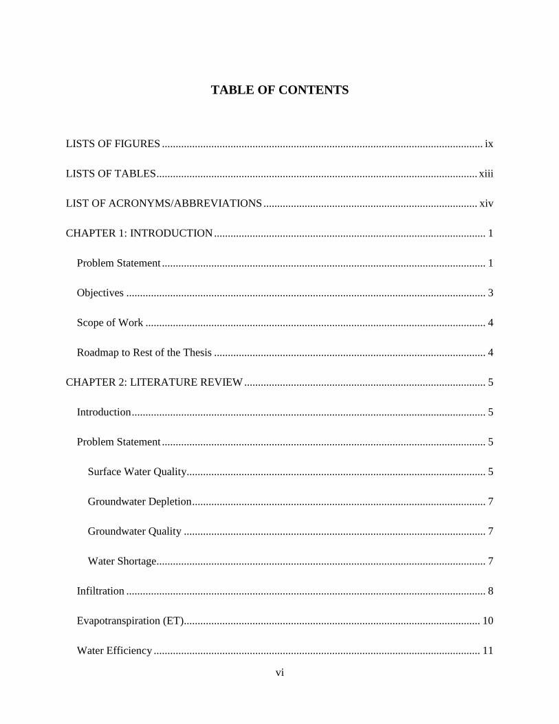
TABLE OF CONTENTS

LISTS OF FIGURES ..................................................................................................................... ix

LISTS OF TABLES ..................................................................................................................... xiii

LIST OF ACRONYMS/ABBREVIATIONS .............................................................................. xiv

CHAPTER 1: INTRODUCTION ................................................................................................... 1

Problem Statement ...................................................................................................................... 1

Objectives ................................................................................................................................... 3

Scope of Work ............................................................................................................................ 4

Roadmap to Rest of the Thesis ................................................................................................... 4

CHAPTER 2: LITERATURE REVIEW ........................................................................................ 5

Introduction ................................................................................................................................. 5

Problem Statement ...................................................................................................................... 5

Surface Water Quality............................................................................................................. 5

Groundwater Depletion ........................................................................................................... 7

Groundwater Quality .............................................................................................................. 7

Water Shortage........................................................................................................................ 7

Infiltration ................................................................................................................................... 8

Evapotranspiration (ET)............................................................................................................ 10

Water Efficiency ....................................................................................................................... 11

vii

Reuse Water Systems ................................................................................................................ 12

Computer Software ................................................................................................................... 13

BMPTRAINS ........................................................................................................................ 14

CUP+ .................................................................................................................................... 15

Soil Properties ........................................................................................................................... 16

Structural performance of HDPE pipes .................................................................................... 17

Design Methodology ............................................................................................................. 17

Polyethylene Pipes ................................................................................................................ 22

Load Effects .......................................................................................................................... 22

HDPE Pipes Systems ............................................................................................................ 24

List of Expected Contributions ................................................................................................. 25

Model .................................................................................................................................... 25

Laboratory Testing ................................................................................................................ 25

CHAPTER 3: METHODOLOGY ................................................................................................ 27

PIPE- R Model .......................................................................................................................... 27

Reservoir ............................................................................................................................... 28

Surface Layer ........................................................................................................................ 31

Drainfield .............................................................................................................................. 34

Strength Testing ........................................................................................................................ 35

viii


Field Testing ......................................................................................................................... 43

CHAPTER 4: RESULTS .............................................................................................................. 56

PIPE-R Model: Example Problem ............................................................................................ 56

Structural Test ........................................................................................................................... 77


Field testing ........................................................................................................................... 88

CHAPTER 5: CONCLUSION ..................................................................................................... 99

APPENDIX A: SYSTEM AVERAGE DEFORMATION VERSUS NUMBER OF RUNS .... 101

APPENDIX B: SENSOR MEASUREMENTS .......................................................................... 104

REFERENCES ........................................................................................................................... 108

ix

LISTS OF FIGURES

Figure 1. Example of REV Curve ................................................................................................. 12

Figure 2. Green Roof System Boundaries .................................................................................... 13

Figure 3. Worksheet with different treatment analysis options .................................................... 14

Figure 4: Input page of the program CUP+ .................................................................................. 15

Figure 5. Diagram of the system ................................................................................................... 27

Figure 6. System boundaries ......................................................................................................... 28

Figure 7. Mass balance diagram for the Reservoir ....................................................................... 29

Figure 8. Mass balance of top surface layer. ................................................................................ 32

Figure 9. System boundary of the Drainfield................................................................................ 34

Figure 10. a. Single pipe before testing; b. Pipe is slightly deformed; c. Pipe is significantly

deformed; d. Pipe is severely deformed ........................................................................................ 37

Figure 11.a. Single BPU before testing; b. Two-Level BPU before testing with top plate .......... 40

Figure 12. One level system of the 37 in. long BPU’s ................................................................. 41

Figure 13. Three level system of the 37 in. long BPU’s ............................................................... 42

Figure 14. Laser position sensor used for individual measurements ............................................ 42

Figure 15. Setup for individual measurements ............................................................................. 43

Figure 16. Plan view of the site .................................................................................................... 44

Figure 17. Section A-A ................................................................................................................. 44

Figure 18.a. Excavated holes; b. Vibratory machine used for compaction; c. System being put

into the holes; d. View of finished testing site .............................................................................. 45

Figure 19. Section view of system 1 ............................................................................................. 46

x



Figure 22. Concrete housing structure for the sensor ................................................................... 48

Figure 23.a. 2 rear axles and a dead axle; b. Two rear axles following the blue lines; c. Rear view

of the truck driving away from the sensor’s location ................................................................... 49

Figure 24. Location of tires with respect to sensor ....................................................................... 49

Figure 25. Connection between sensor and steel bar .................................................................... 50

Figure 26. Sensor used for field test ............................................................................................. 51

Figure 27. Pictures of the DAQ with and without the cap ............................................................ 52

Figure 28. Pictures of the terminal block (left) and CompactDAQ Chassis connected to the DAQ

(right) ............................................................................................................................................ 52

Figure 29. Power supply ............................................................................................................... 53

Figure 30. Diagram of the connections in LabVIEW ................................................................... 54

Figure 31. Example of the sensor’s reading.................................................................................. 54

Figure 32. Conduit from housing structure to DAQ ..................................................................... 55

Figure 33. Manual calculation feature was activated .................................................................... 57

Figure 34. Introduction page worksheet ....................................................................................... 57

Figure 35. General Instructions worksheet ................................................................................... 58

Figure 36: Instructions to obtain historical data from NOAA ...................................................... 58

Figure 37. NOAA website for requesting precipitation data ........................................................ 59

Figure 38. NOAA website showing the desired location ............................................................. 60

Figure 39. NOAA website where the output format was selected ................................................ 60

Figure 40. NOAA website notice displayed if data selected was not available. .......................... 60

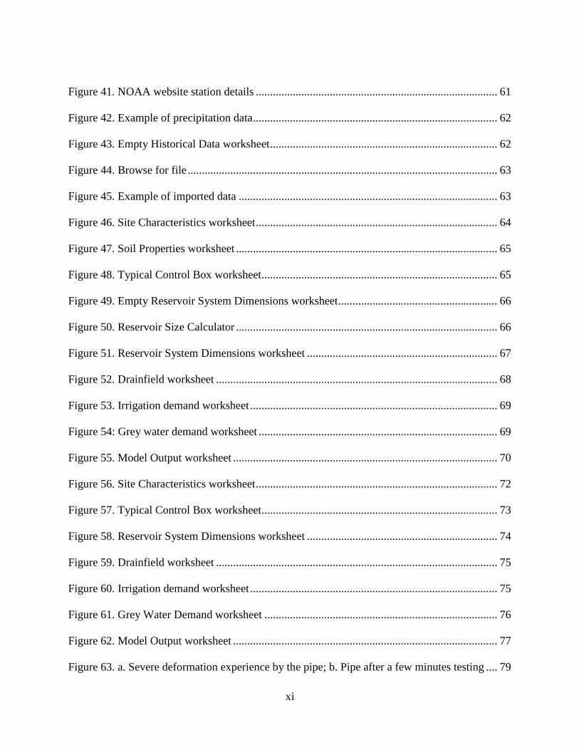
xi

Figure 41. NOAA website station details ..................................................................................... 61

Figure 42. Example of precipitation data ...................................................................................... 62

Figure 43. Empty Historical Data worksheet ................................................................................ 62

Figure 44. Browse for file ............................................................................................................. 63

Figure 45. Example of imported data ........................................................................................... 63

Figure 46. Site Characteristics worksheet ..................................................................................... 64

Figure 47. Soil Properties worksheet ............................................................................................ 65

Figure 48. Typical Control Box worksheet................................................................................... 65

Figure 49. Empty Reservoir System Dimensions worksheet ........................................................ 66

Figure 50. Reservoir Size Calculator ............................................................................................ 66

Figure 51. Reservoir System Dimensions worksheet ................................................................... 67

Figure 52. Drainfield worksheet ................................................................................................... 68

Figure 53. Irrigation demand worksheet ....................................................................................... 69

Figure 54: Grey water demand worksheet .................................................................................... 69

Figure 55. Model Output worksheet ............................................................................................. 70

Figure 56. Site Characteristics worksheet ..................................................................................... 72

Figure 57. Typical Control Box worksheet................................................................................... 73

Figure 58. Reservoir System Dimensions worksheet ................................................................... 74

Figure 59. Drainfield worksheet ................................................................................................... 75

Figure 60. Irrigation demand worksheet ....................................................................................... 75

Figure 61. Grey Water Demand worksheet .................................................................................. 76

Figure 62. Model Output worksheet ............................................................................................. 77

Figure 63. a. Severe deformation experience by the pipe; b. Pipe after a few minutes testing .... 79

xii

Figure 64. Load-deflection summary plot .................................................................................... 80

Figure 65. One level system of the 37 in. long BPU’s ................................................................. 84

Figure 66. Average load-deflection plots each level .................................................................... 85

Figure 67. Plot of sensor 2 showing noise in the data .................................................................. 89

Figure 68. Data extracted from Sensor 1 ...................................................................................... 90

Figure 69. Method used to calculate net deformations ................................................................. 91

Figure 70. Cover thickness vs. average deformation of the systems ............................................ 93

Figure 71. Deformation on milling surface................................................................................... 94

Figure 72. Average deformation in each run for sensor 5. ........................................................... 95

Figure 73. Average deformation in each run for sensor 6. ........................................................... 95

Figure 74. Boxplot of deformations versus sensors. ..................................................................... 96

xiii

LISTS OF TABLES

Table 1: Summary of PS for single pipes ..................................................................................... 78

Table 2. Average values for each level and PS reduction ............................................................. 81

Table 3. Comparison between PS methods................................................................................... 82

Table 4. PS values for 37 inches long BPU’s ............................................................................... 86

Table 5. PS values for the long BPU’s ......................................................................................... 87

Table 6. Average deformations for each run in sensors 1 and 2 ................................................... 92



xiv

LIST OF ACRONYMS/ABBREVIATIONS

A total watershed of area (ft2)

AASHTO American Association of State Highway and Transportation Officials

C rational coefficient of watershed

CWA Clear Water Act

EIA effective impervious area (ft2); CA

EPA Environmental Protection Agency

F cumulative infiltration (in).

FAO Food and Agriculture Organization

FEM Finite element method

fp infiltration capacity (in/hr)

Fp Cumulative infiltration until ponding event (in)

HDPE High-density polyethylene

k crop consumptive use coefficient

Ks saturated hydraulic conductivity (in/hr)

Md initial moisture content deficit (|ϴf- ϴi|)

p percent of daily daytime (p).

REV rate-efficiency-volume

S capillary suction at the wetting front (in)

Sav average capillary suction at the wetting front (in).

SCS Soil Conservation Service

t average monthly temperature

t time (hr.)

xv

tp time duration until ponding event (hr.).

ϴf moisture content

ϴi initial moisture content

1

CHAPTER 1: INTRODUCTION

Problem Statement

Water is used every day for an infinite amount of activities thanks to efficient water

network systems that are often not noticed by the general population. There are several problems

arising from the use of water, such as decrease in water quality, groundwater depletion and water

scarcity. A sufficient supply of water is just as important as the functionality of the pipes

delivering it. An evaluation of the integrity of pipes previously installed in the field have shown

that great amount of them need to be replaced or maintained (Folkman and Moser 2002). Pipes

buried underground are important to transport water wherever it is needed and a deep

understanding of their structural properties is required in order to avoid failure.

Certain places around the world are not privileged with a simple access to water or just

do not have the right infrastructure to collect water. This serious problem needs investigation and

efforts geared to minimize the problem as much as possible. Therefore, research on the problem

is necessary to gain knowledge about possible solutions. In addition, the shortage of water is

decreasing the accessibility of water in some circumstances. For example, the depth of water

level in underground aquifers has been increasing throughout the years. The reason for this

phenomenon is the overexploitation of this resource, extracting water from the aquifer at a much

faster rate than it can be replenished. The depletion of the aquifer can be mitigated by reducing

the amount of water extracted through an adequately designed stormwater harvesting system

Nutrient loading from stormwater runoff negatively affects the quality of surface water

body, which then creates a variety of negative consequences to the surrounding environment

(Pinckney et al. 2001). The most common nutrients present in lakes are phosphorus (P) and

2

nitrogen (N) (Minnesota Pollution Control Agency 2008). Some of the events that lead to

nutrient loading are deforestation, fertilizers, human and animal wastes. Multiples studies have

concluded that nutrient loading is the main source for the increase algae bloom in a water body

(Brookes and Carey 2011). Lee et al. (2001) stated that algae bloom causes detrimental effects

on animals and the aquatic ecosystem because of their release of toxins and the greater effort

needed while filtrating pollutants out of the water. Therefore, it is important to control the rate of

nutrient loading in water bodies, and one possible solution is to limit the amount of water

discharged from point and non-point sources.

Water harvesting systems could minimize or eliminate problems related to the excessive

water demand by capturing some of it during rainfall events. In addition, the reduction of the

amount of water discharged leads to corresponding decrease in the transport of sediment, which

eventually keep the water quality at acceptable standards. The applications of water harvesting

systems can be implemented for a wide range of tasks as long as a proper designs are performed.

An effective water harvesting systems needs also to be structurally sound. Therefore,

another aspect that needs to be inspected, besides the water harvesting capabilities, are the

structural properties of the pipes that form the water harvesting system. The structural properties

of the pipes need to withstand the loads from overburden earth pressure and vehicular loading.

Polyethylene pipes are currently used for underground applications in the United States

(Krishnaswamy 2005, Motahari and Abolmaali 2009). Polyethylene is a viscoelastic material,

which means that its structural properties are dependent to time (Bilgin 2013). Plastic pipes often

experience large deformations due to stress relaxation, a typical behavior for viscoelastic

materials. These deformations are considered extreme once the size or shape of a pipe is severely

altered. A study showed that 63% of the pipes used in the United States suffer greater degrees of

3

deformation compared to the allowable limit specified in AASHTO codes (Folkman and Moser

2002, Barker and Puckett 2013). The study also showed that the maximum vertical deformations

found in pipes were 22.5% with an average maximum vertical deformation of 7.2%. In order to

avoid losses and/or failures, their structural performance needs to be well understood prior to the

design stage.

Objectives

The reduction of water shortages in different fields can be accomplished by the use of

reuse water applications. EPA defines this procedure as “reusing treated wastewater for

beneficial purposes such as agricultural and landscape irrigation, industrial processes, toilet

flushing, and replenishing a ground water basin (referred to as ground water recharge)” (EPA

2013). Sophisticated water harvesting systems have been created to alleviate some of the demand

and maximize its use. Different models related to a variety of applications have been done in the

past to predict the performance of these systems (Dixon et al. 1999). In this study, the topics

related to water harvesting and structural performance of pipes will be investigated. In order to

do so, a model will be created to account for several parameters and predict its water harvesting

efficiency. Regarding the model parameters, the ranges of variation includes data related to the

physical size, location, type of soils, quantity of reuse water demand and so on. The other section

of this study corresponds to laboratory and field testing needed to estimate the ability of the pipe

to withstand loads from the earth pressure and vehicular loading. To accomplish the structural

evaluation, results from loading tests performed on the pipe will be compared minimum

requirements specified on AASHTO (2012). The specific objectives are:

1. Create a model to simulate the water harvesting performance of PIPE-R System

4

2. Perform laboratory and field testing to predict the structural integrity of buried

high-density polyethylene (HDPE) pipes.

Scope of Work

Plastic Tubing Industries, Inc. have crafted an underground water harvesting system

called PIPE-R Model and the UCF Stormwater Management Academy has developed an EXCEL

based model in order to simulate its performance to store and redistribute water for an average

year for any location where hourly precipitation data exists. This model will also help the user

adjust the characteristics of the system in order to achieve a particular efficiency desired. In

addition to the model, laboratory and field testing will be conducted to predict the structural

performance of the pipes under the loading conditions.

Roadmap to Rest of the Thesis

The Chapter 1 of this thesis provides an introduction to some of the water related issues

addressed by the implementation of the proposed system such as surface water quality, water

scarcity and groundwater depletion. Another problem discussed is the structural integrity of

underground HDPE pipes used for water harvesting. The main objective and scope of the work

are located in this section, as well as roadmap of the thesis in order to help the reader. Chapter 2

presents a compilation of studies evaluated prior to initiating this project. These studies include a

range of concepts such, infiltration, evapotranspiration, water demands, load calculations and

different structural properties regarding HDPE pipes. A hypothesis is also included in

conjunction with the impact of the results. Chapter 3 is describes procedures and tools utilized to

perform this study. Chapter 4 presents all the results of this study along with a discussion based

on them. Chapter 5 offers conclusions from the results, a brief statement of the main points of the

study and recommendations for upcoming work.

5

CHAPTER 2: LITERATURE REVIEW

Introduction

Water scarcity is one of the main problems experienced in several places around the

world. One focus of this study is to analyze the water harvesting performance of an underground

pipe system. Having a greater understanding of the pipe system will be useful to design more

effective systems that would achieve the desired criteria. This chapter presents discussions on the

stormwater harvesting as it relates to water quality, groundwater depletion and water shortage.

Consequently, to minimize these issues this study will discuss the mass balance of water along

with the multiple processes that water experiences. Processes of infiltration and

evapotranspiration (ET) often occur due to the interaction of water with soils and changes in the

temperature. This section will later explain how infiltration and ET are calculated along with the

methods to evaluate water-harvesting operations.

In addition, structural properties of the pipe system need to be adequate for serviceability

purposes and to avoid failure. Thus, the second part of this section will address the issue of

structural integrity of buried pipes. The study on the behavior of buried pipes requires the

understanding of the material type and manufacturing process to determine the response to

applied loads. This section discusses common methods for the calculation of dead and live loads,

as well as the associated theories that describe structural behavior of buried pipes.

Problem Statement

Surface Water Quality

Surface runoff is generated during rainfall events on surfaces that are saturated with

water or consist of impervious layer that does not have any significant ability to absorb water.

6

Stormwater runoff, which transports soil particles and other materials, is considered a Nonpoint

Source Pollution (Harbor 1999) and a primary source of contaminants in water bodies in the

United States (Langeveld et al. 2012). One example of a contaminant is phosphorus, which

controls the growth of plants in water bodies and excessive amounts of it could produce

eutrophication (Hardin 2006). Other contaminants have the ability to affect the pH of water

bodies which would acidify water and cause death to aquatic organisms (Leuven et al. 1986).

There are particular ways to quantify the quality of discharged water such as alkalinity,

biological oxygen demand (BOD), nitrogenous oxygen demand (NOD) and turbidity (Metcalf et

al. 1972).

Turbidity, which is a measure of water clarity, is increased by soil particles present in

water bodies. According to Paaijmans et al. (2008), significant degree of turbidity present in

water is linked to higher temperatures, which in turn increases the rate of reproduction of algae.

Harmful algal blooms often decrease the dissolved oxygen demand that can be detrimental to

fish and other aquatic species (Paaijmans et al. 2008). To control and minimize the presence of

contaminants in water bodies, regulations such as the Clean Water Act have been implement by

environmental agencies.

Regulations: Clean Water Act

In 1972, the amendment of the Federal Water Pollution Act was renamed as the Clean

Water Act (CWA) and had the responsibility to control the discharge of pollutants and quality of

surface waters discharged by construction projects, which disturbed one or more acres of land. A

common benchmark of the quality of discharged water is known as Total Maximum Daily Load

(TMDL), which is the maximum acceptable amount of specific pollutants that can enter a water

body. The CWA also issues National Pollutant Discharge Elimination System (NPDES) permits

7

to construction sites as long as their stormwater effluents follow the Environmental Protection

Agency’s (EPA) minimum standards for water quality (EPA 2011). The process for the provision

of permits involves the evaluation of a Storm Water Pollution Prevention Plan (SWPPP), which

explains the details of the specific erosion and sediment control plan utilized on a project site.

Groundwater Depletion

Aquifers are suitable sources of fresh water but the amount of water in them is finite and

extraction rates that are higher than the aquifer’s recharge rates would end up in depletion

(Gleeson et al. 2010). The study conducted by Gleeson et al. (2010) also stated that a decrease of

water levels in an aquifer can have damaging consequences such as drastic changes in stream

flows and ecosystems dependent of it. Another study conducted on the Ogallala Aquifer in

United States and other major aquifers showed that depletion has been occurring and that yearly

volumes of depletion in the U.S. are about 32 km3/acre (Gutentag 1984, Wada et al. 2010).

Groundwater Quality

Although many researchers have studied overexploitation of aquifers, only few studies

have been done related to the quality of water within the aquifers. A study conducted by

Chaudhuri and Ale (2014) was to understand patterns of water quality and salinization

throughout different regions of the Ogallala aquifer from the year 1960 to 2010. The study

concluded that salinization increased with time and the contributing factors were natural and

anthropogenic processes. The study also found the water to be contaminated with particular

nutrient concentration in different regions and depths.

Water Shortage

Water shortage has been considered as a major issue and the main causes are the growing

population, increasing irrigation areas, economic growth and water management (Wada et al.

8

2010, Zarghami and Akbariyeh 2012). Lack of fresh water is directly related to several problems

today such as health, poverty and water management (Rijsberman 2006). Rijsberman (2006)

futher stated “when an individual does not have access to safe and affordable water to satisfy her

or his needs for drinking, washing or their livelihoods we call that person water insecure”.

Approximately 1.2 billion people suffer from water scarvity and an adittional 500 million are

being directed to this condition (Watkins 2006). Increasing demands by growing populations

have been attenuated by extracting water from aquifers and freshwater sources, but these

approaches will eventually reach their limits.

Infiltration

Infiltration, has been studied by several researchers which has led to the existence of

various models to predict the amount of water being infiltrated to the ground (Philip 1957,

Morel‐Seytoux and Khanji 1974). Although much effort has been put to infiltration, most models

are not successful in forecasting the magnitude of infiltration due to variations in the soil layers.

Some methods regarding infiltration such as Holtan (1961), provide approximate results but have

the problem of variables that possess no physical significance or calculations that do not provide

all the results desired. Other infiltration models such as model from Philip (1957) required

considerable effort in computing some of its variables. The equation created by Green and Ampt

(1911), later modified by researchers (Chu 1978, Serrano 2001), has been one of the most

effective models to predict infiltration due to simplicity and use of physical variables. The

Green-Ampt equation is:

fp = K [1 + (MdS

F)] (1)

9

where: fp = infiltration capacity (in/hr); K = saturated hydraulic conductivity (in/hr); Md = initial

moisture content deficit (|ϴf- ϴi|); ϴf:= moisture content; ϴi = initial moisture content; S =

capillary suction at the wetting front (in); F = cumulative infiltration (in).

The Green-Ampt equation (see Equation (1) has been proven to produce accurate results,

but it is important to consider the exact time when water starts to pond since it provides

relationships between the infiltration rate and the infiltration capacity (Liu et al. 2010). Several

methods were based from the Green-Ampt equation, for example, a common equation for the

infiltration rate under a ponded surface as presented by Mein and Larson (1971) in Equation (2):

fp =dFp

dt= K +

KSM

Fp for t > tp (2)

where: Fp = Cumulative infiltration until ponding event (in); t = time (hr.); t = time duration until

ponding event (hr.).

However, a limitation of the Green-Ampt equation was that the equation was separated in

stages: before and after ponding. Chu (1978) proposed an approach that could integrate the

different stages, in other words, include the amount of water infiltrated before ponding. The

author utilized methods developed by Mein and Larson (1971) for steady rainfall and extended it

to successfully simulate unsteady rainfall events. The main concept about this method is to shift

the time by a parameter called pseudotime (equivalent time to infiltrate Fp under ponded surface

conditions). The same study compared the measurements between the approach suggested by

Chu and actual values measured in the field, and confirmed that the use of the pseudotime

provided accurate results. As long as the rainfall intensity is less that than the infiltration rate,

there will be no ponding and all water is infiltrated. Once the top soil is ponded, the rainfall

intensity does not affect the rate of infiltration, which increases up to a maximum value known

10

as the infiltration capacity of a particular soil. Since infiltration values are implicit in the

formulas, several mathematical steps needed to be calculated before obtaining a solution.

Consequently, Chu (1978) integrated equation (2) to obtain the value of cumulative

infiltration. The corresponding equation can be seen below (See Equation (3):

F/SM − ln(1 + F/SM) = K(t − tp − ts)/𝑆𝑀 (3)

where: Sav = average capillary suction at the wetting front (in).

Evapotranspiration (ET)

Since irrigation accounts for the greatest amount of water use, understanding evaporation is

fundamental for water resources planning. One equation widely used by professionals for

assessing reference evapotranspiration (ET) is the Penman-Monteith. This method requires

hourly or daily measurements of variables such as temperature, radiation, wind speed, and

humidity. The need for the variables just mentioned will require lots of effort which can

sometimes create a problem. Although the Penman-Monteith equation might be considered as

the most accurate method, the Blaney-Criddle equation tends to be most widely used approach

due to simplicity. The only weather data required by the Blaney-Criddle equation to estimate ET

is air temperature measurements. The original form of the Blaney-Criddle equation was modified

by Soil Conservation Service (SCS) (SCS 1970) and Food and Agriculture Organization (FAO)

of the United Nations (J. Doorenbos and Pruitt 1984).

The equation of Blaney-Criddle involves three variables: the crop consumptive use

coefficient (k), the average monthly temperature (t) and the percent of daily daytime (p). The

equation can be seen below (See Equation(4):

u =ktp

100 (4)

11

where: u = monthly evaporation (in.); k = monthly ET coefficient; t = mean monthly temp (˚F), p

= monthly % annual daytime hours

One limitation of this equation is the difficulty to predict accurate values of

evapotranspiration in places with high elevation. Such high elevation locations exhibit lower

temperature during the night and force the average daily temperature to drop even though the

solar radiation remains stable. In order to increase accuracy, k values were established for

different growing stages of the subjected crops. A study provided an alternative approach where

available weather data can be used to obtain more accurate results with the Blaney-Criddle

equation (Juday et al. 2011).

Water Efficiency

It has been proposed that wet ponds should reuse some of their water as an alternative for

irrigation instead of discharging it downstream (Wanielista et al. 1991). The process of reusing

water is beneficial since it can help reduce the volume of water, which will lead to a decrease in

the local water loss and amount of discharged pollutants to water bodies. Numerous mass

balance studies were conducted on ponds which incorporate reuse systems with rainfall data, and

the outcomes were used to develop the rate-efficiency-volume (REV) curves (Wanielista et al.

1991).

REV = 1 −Reuse Water Vol.

EIA (5)

where: EIA = effective impervious area (ft2); EIA = CA; C = rational coefficient of watershed; A

= total watershed of area (ft2).

12

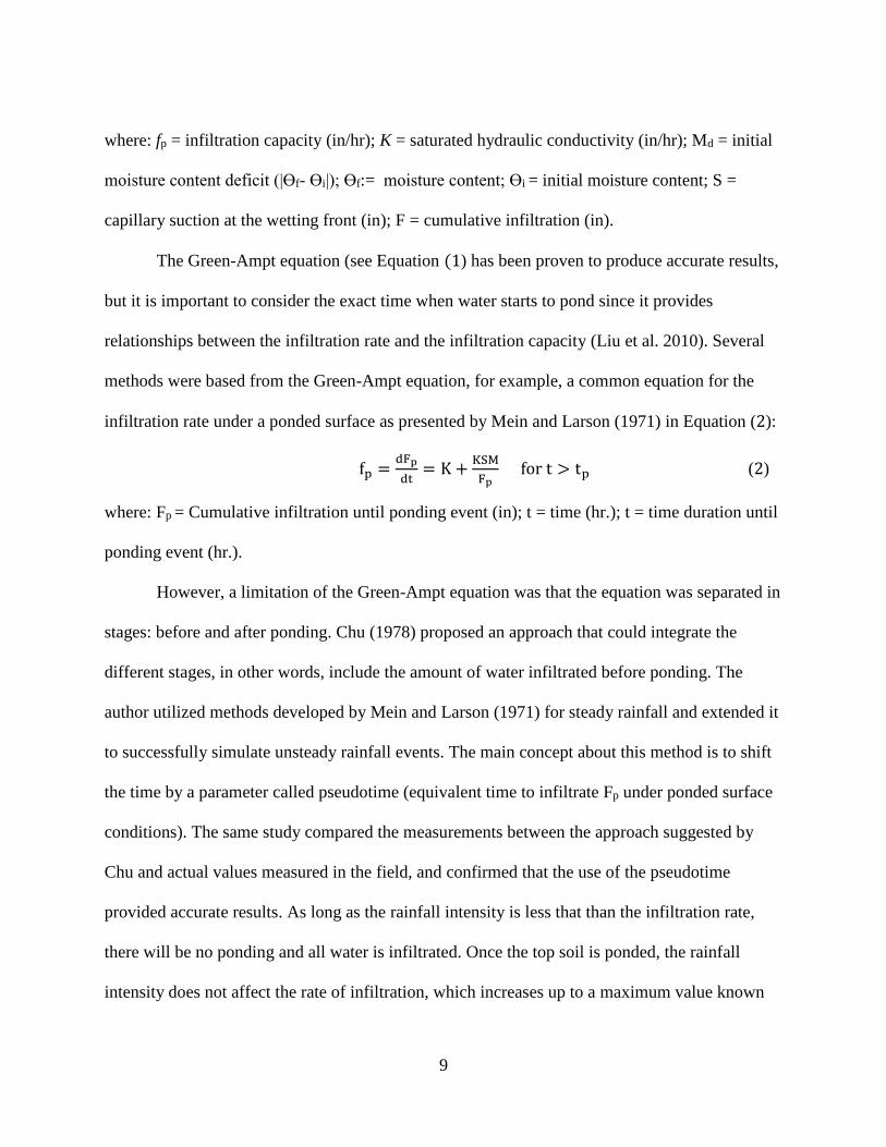
Basically, the REV Curve values are the percent of water reused from the total amount of

water introduced to the system. An example of a REV curve from a Tallahassee rainfall station

was extracted from the study by Wanielista et al. (1991), and is shown below :

Figure 1. Example of REV Curve (Wanielista et al. 1991)

Reuse Water Systems

Hardin et al. (2012) conducted a study to understand the performance of green roofs that

infiltrated stormwater runoff with the additional use of a cistern. The main goals of green roofs

are to reduce the amount of pollutants in the incoming water and to hold water for longer

periods. Increasing the detention time of water helps increase evapotranspiration and reduces the

amount of water discharged. In order to determine how much water infiltrated from green roofs

13

including the use of a cistern, Hardin used a mass balance approach which involved the rates of

evapotranspiration (ET), input water (I) and precipitation (P) the Media Storage (MS) .

Figure 2. Green Roof System Boundaries (Hardin 2006)

Figure 2 shows the use of boundaries around the green roof media storage and then

another around the overall system in order to calculate the efficiency of the system. The

efficiency equation, slightly similar to the REV curves equation, were calculated by dividing the

amount of water retained by the volume of rainfall and water input from the cistern (Wanielista

et al. 1991, Hardin 2006).

Computer Software

There are some software programs created to provide a rapid and efficient way to

determine the performance of certain systems through a set of automated calculations. Brief

discussions on two BMPTRAINS and CUP+, software purposes and capabilities are presented.

14

BMPTRAINS

This Excel based model was created to assess stormwater runoff nutrient loads and the

removal performance of various BMPs (best management practices) based on recent research

findings in the State of Florida (Harper and Baker 2007, Wanielista et al. 2014). A BMP is a

control structural system that that serves as an economical element to reduce the pollution in

water to meet water quality standards. There is a wide variety of BMPs and this program allows

private and governmental agencies to have a good understanding of their functions and benefits

of the BMP’s working together. Figure 3 shows an input worksheet screenshot of the

BMPTRAINS model where the user can select target reduction efficiency for nutrients as

nitrogen and phosphorus along with different treatment methods that can be implemented at the

bottom of the worksheet page.

Figure 3. Worksheet with different treatment analysis options (Wanielista et al. 2014).

15

CUP+

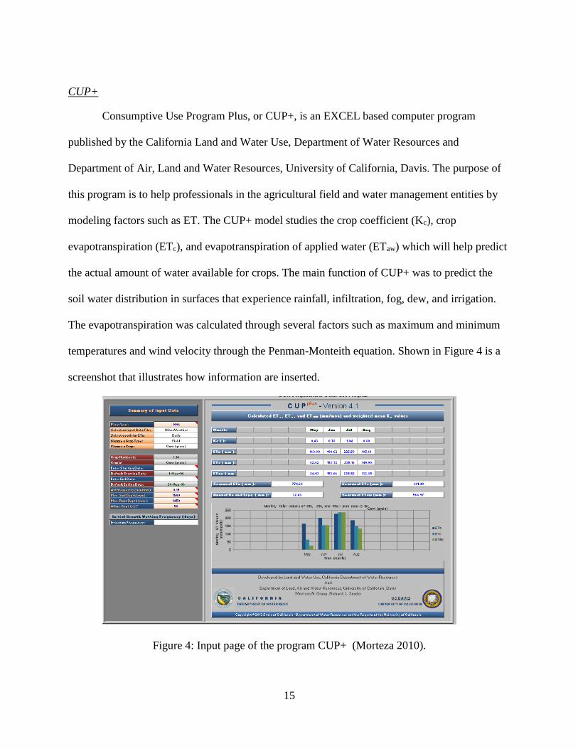
Consumptive Use Program Plus, or CUP+, is an EXCEL based computer program

published by the California Land and Water Use, Department of Water Resources and

Department of Air, Land and Water Resources, University of California, Davis. The purpose of

this program is to help professionals in the agricultural field and water management entities by

modeling factors such as ET. The CUP+ model studies the crop coefficient (Kc), crop

evapotranspiration (ETc), and evapotranspiration of applied water (ETaw) which will help predict

the actual amount of water available for crops. The main function of CUP+ was to predict the

soil water distribution in surfaces that experience rainfall, infiltration, fog, dew, and irrigation.

The evapotranspiration was calculated through several factors such as maximum and minimum

temperatures and wind velocity through the Penman-Monteith equation. Shown in Figure 4 is a

screenshot that illustrates how information are inserted.

Figure 4: Input page of the program CUP+ (Morteza 2010).

16

The method used by the program to determine some of such average climate values and

other evaporation rates for monthly data is curve fitting, a method commonly used for this

application (Cesaraccio et al. 2001). For general cases where a crop is present, a Kc value is

selected based on the specific crop used. The value of Kc, along with the crop evapotranspiration

varies throughout the growing period of the crop.

Some of the variables that need to be inserted by the users in the program are crop type

(field, deciduous, subtropical), the period duration, ET contribution from fog and dew and so on.

Frequency of irrigation events, effective rooting depth, monthly and daily weather data are

factors considered to make predictions about the water balance. The net water applied to crops

(ETaw) is also important when growers need to plan their actions regarding their crops.

Soil Properties

Understanding the amount of water that can be held by a soil is very important while

managing tasks related to irrigation such as arrangement design, schedule, crop selection and

magnitude. The water holding capacity is related to the field water capacity and there are various

procedures utilized to determine their magnitude (Asgarzadeh et al. 2014). Methods used to

determine field water capacity can be done by field measurements, laboratory testing or

empirical methods based on soil properties. In a study done to compare the results found through

laboratory testing versus field measurements, Gebregiorgis and Savage (2007) concluded that

values found in the laboratory were quite different from the ones in the field. The authors

explained that the differences could be due to a variety of reasons such as the sample being

altered from the time it was taken in the field, the different nature of each method and soil

17

variability. Water demands for irrigation are sometimes estimated with water mass balance

equations and an important factor is soil porosity.

Porosity studies have shown that a rapid infiltration process increases directly with the

degree of connection of pores in the soil column (McIntyre and Sleeman 1982). Helalia (1993)

studied the relationship between different soil properties, such as textural and structural, and the

in situ infiltration rate. At the end of the experiment, it was determined that effective porosity

produces the strongest correlation with the infiltration and that the rest of the variables do not

increase the accuracy.

Structural performance of HDPE pipes

Design Methodology

Pipes are often classified as flexible or rigid material based on how they behave under a

load. Rigid pipes obtain their strength from the material itself such as concrete of steel

(Jeyapalan and Boldon 1986). Even though flexible pipes are made out of materials with lower

stiffness than the rigid pipes, they are better at distributing the load to the surrounding soil. In

addition, flexible pipes have the ability experience higher deformations than the rigid pipes

without encountering failure.

According to Kang et al. (2009), some benefits of flexible pipes are light weight, less

amount of joints needed, much greater resistance to corrosion and less difficulty during

construction stages. Flexible pipes have a greater contact area with the soil while transferring

loads, unlike the rigid pipe that has a concentrated contact area where the interaction occurs. This

interactions present an advantage for flexible pipes because it allows them to be used at much

deeper locations than rigid pipes.

18

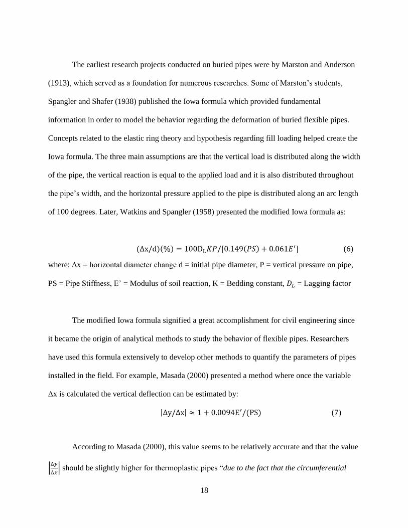
The earliest research projects conducted on buried pipes were by Marston and Anderson

(1913), which served as a foundation for numerous researches. Some of Marston’s students,

Spangler and Shafer (1938) published the Iowa formula which provided fundamental

information in order to model the behavior regarding the deformation of buried flexible pipes.

Concepts related to the elastic ring theory and hypothesis regarding fill loading helped create the

Iowa formula. The three main assumptions are that the vertical load is distributed along the width

of the pipe, the vertical reaction is equal to the applied load and it is also distributed throughout

the pipe’s width, and the horizontal pressure applied to the pipe is distributed along an arc length

of 100 degrees. Later, Watkins and Spangler (1958) presented the modified Iowa formula as:

(∆x/d)(%) = 100DL𝐾𝑃/[0.149(𝑃𝑆) + 0.061𝐸′] (6)

where: Δx = horizontal diameter change d = initial pipe diameter, P = vertical pressure on pipe,

PS = Pipe Stiffness, E’ = Modulus of soil reaction, K = Bedding constant, 𝐷𝐿 = Lagging factor

The modified Iowa formula signified a great accomplishment for civil engineering since

it became the origin of analytical methods to study the behavior of flexible pipes. Researchers

have used this formula extensively to develop other methods to quantify the parameters of pipes

installed in the field. For example, Masada (2000) presented a method where once the variable

Δx is calculated the vertical deflection can be estimated by:

|∆y/∆x| ≈ 1 + 0.0094E′/(PS) (7)

According to Masada (2000), this value seems to be relatively accurate and that the value

|∆𝑦

∆𝑥| should be slightly higher for thermoplastic pipes “due to the fact that the circumferential

19

shortening of the pipe under loading tends to make the horizontal deflection smaller and the

vertical deflection larger when compared to the deflections of a corrugated metal pipe with the

same ring stiffness” (Masada 2000). Masada (2000) also stated that other methods proposed by

Burns and Richard (1964) or Hoeg (1966) are more accurate but the Spangler equation is more

widely used due to its simple calculations.

AASHTO Design Method

The AASHTO Design is commonly used to model the magnitude of dead and live loads

applied to the pipe buried underground (AASHTO 2012). Once live and dead loads are

determined, the thrust on the pipe can be calculated.

Live and dead load equations are used to calculate the theoretical loads that will be

applied to the pipes in the field. In an analysis, both the live and dead loads are factored to

minimize potential errors in design. These load factors are multipliers that were calculated

statistically with the purpose of accounting for any variability of loads and the possibilities of

some miscalculations in the design. Brief explanations will be provided to explain dead and live

loads.

Dead Load

Dead loads, or static loads, are typically non-dynamic weights supported by the structure

itself and remain constant over a long period of time. In the case of a building or roadway

structure, weights of their structural components and utilities are considered dead loads. For the

case of a buried pipe, the dead load is the soil cover laying on top, which includes the pavement

layer. The equation used to estimate the dead load is the soil-prism load expressed in Equation 7.

20

Psp = [H + 0.11(D0/12]γs/144 (8)

where: PSP = soil prism pressure (EV), evaluated at pipe’s horizontal centerline (psi); H = depth

of fill over top of pipe (ft.); D0 = outside diameter of pipe (in); γs = wet unit weight of soil (lbs.

/ft.3 ).

Live Loads

Live loads are dynamic loads on the structure that, in relatively short period of times, can

change locations or not be present in the structure. Examples of live loads can be human

occupancy, furniture for buildings and vehicles for a bridge. A more concise procedure to

calculate live load was adopted from the Report 647 (NCHRP 2010). The principal equation to

determine the service live load applied to an underground pipe is:

WL = MPF(1 + IM)WLL (9)

where: WL = service live load (psi); WMPF = multiple presence factor (1.2); IM = impact factor

(0.33); WLL = live load pressure (psi).

General Factored Load Equation

The general factored load equation that combines all forces applied on the buried

structure is represented by the following equation:

Pf = ηEV(γEVVAF × PSP) + ηLLγLLCLWLL (10)

where: Pf = factored vertical crown pressure (psi); ηEV = load modifier for live loads, AASHTO

21

Art.1.3.2; VAF = Vertical arching factor; PSP = soil prism pressure (EV); ηLL = load modifier as

specified in Article 1.3.2, as they apply to live loads on culverts; γLL = load factor for live load,

as specified in Article 3.4.1; CL = live load distribution coefficient; WL = live load pressure (psi)

Once general factored load equation has been calculated, the thrust per unit length on the

pipe can be calculated. In accordance to AASHTO (2012), the equation to calculate thrust is:

TL = 𝑃𝑓(𝐷𝑜

2) (11)

where: TL= factored thrust per unit length (lbf/ft), Do = outside diameter of pipe (ft), Pf= factored

vertical crown pressure (lbf/ft2)

All equations recently shown above are needed to calculate the theoretical deflection on a

single pipe. The equation to calculate deflection involves variables such as the diameter to

centroid of pipe wall, thrust on the pipe, pipe wall area, fifty-year modulus of elasticity of the

pipe’s material, maximum load factor for Vertical Earth pressure (EV) (AASHTO 2012). The

formula to calculate the theoretical deflection can be found below:

∆= 0.05D −TL𝐷

𝐴𝑒𝑓𝑓𝐸50𝛾𝑝 (12)

where: TL= factored thrust per unit length (lbf/ft); D = diameter to centroid of pipe wall (ft), Aeff

= effective pipe wall area; E50= fifty-year modulus of elasticity; γp = maximum load factor for

Vertical Earth pressure (EV)

22

Polyethylene Pipes Polyethylene pipes have been widely used to replace old pipe systems or build new ones

(Bilgin 2013). Since polyethylene pipes behave as viscoelastic material, their behavior under

stress reflect a combination of elastic and viscous. The relationship between stress and strain is

non-linear and its properties vary depending on temperature, duration of load applied and the

degree of stress inserted. A particular property exhibited by polyethylene pipes is creep and it

represents the time-dependent permanent deformation which in the long-term can produce failure

in the pipe (O'Connor 2011). Polyethylene pipes in general have a higher susceptibility to

temperature changes related to loading stresses. In other words, these pipes will extract or

contract at a higher degree and this can affect the integrity of the whole pipe system.

Load Effects

Plastic pipes often experience large deformations due to stress relaxation, a typical

behavior for viscoelastic materials. According to Motahari and Abolmaali (2009), the

deformations are considered extreme once the size or shape of a pipe is severely altered. The

different cases are classified as: deformation in the x or y axis, ovality, crown flattening, inverse

curvature and bucking. A study showed that 63% of the pipes used in the United States suffer

greater degrees of deformation compared to the allowable one specified in the AASHTO codes

(Barker and Puckett 2013). Furthermore, the maximum deformations found in pipes were 22.5%

and the average maximum deformation was 7.2%.

Kang et al. (2009) studied the short-term and long-term effects of the HDPE pipes by

using finite element method (FEM) and current design equations (AASHTO 2012). Some of the

findings found in the study conducted by Kang et al. (2009) were that the earth loads on this type

of structure greatly vary depending on the time related properties. This project also proposed that

23

observed reduction in the elastic modulus were related to decreased earth loads. Results found

through a FEM software called ABAQUS were closely related to methods proposed by Burns

and Richard (1964) but were significantly smaller than the ones produced by Spangler and

Shafer (1938). Lately, HDPE pipes have been used for stormwater detention system therefor

their behavior in this type of design needs to be understood. Some conducted experiments

increasing the strength of the pipe by adding additional components to it (Shijian et al. 2002,

Khatri et al. 2013).

By combining the strength of plastic and steel, steel reinforced high-density polyethylene

(SRHDPE) pipes should overcome the problem experienced by each material alone. The ribs of

the pipe are formed by high strength steel that provides significant strength and stiffness. In order

to have a deeper understanding of this component, Khatri et al. (2013) performed a study related

to the compressive behavior of the pipes under static loads. Khatri et al. (2013) concluded that

the pipes met the minimum requirement according to ASTM F2562 and that yielding was

observed at about 6% vertical deflection and the maximum loads were experienced at 10%

deflection. The last finding corresponded to a vertical deflection that was about 1.25 time greater

than the horizontal deflection. The last few research projects consisted on studying behavior of

pipes under dead loads but the effects of live loads are also critical for a proper design(Lay and

Brachman 2013).

Results of a study performed by Arockiasamy et al. (2006)demonstrated that additional 6

inches of cover would reduce about 2 to 3 times the vertical pressure applied to the crown of pipe

in HDPE pipes of large diameter compared to the smaller ones. The deformations measured in

the field were compared with the Spangler equation, the modified Meyerhof formula and two

24

FEM software programs (CANDE and ANSYS). The results supported that ANSYS created the

closest approximation to values found in the field.

Faragher et al. (2000) performed research studies related to the behavior of plastic pipes

under repeated vehicular loads. The study consisted on passing trucks 1,000 rounds over a road

that contained buried pipes. The findings showed that the stress in these pipes rapidly increase in

the initial stages but later the effects decreased until the pipes reached a point where they became

stable. The studies proposed curves that would help understand the long-term effects of plastic

buried pipes. In addition to tests conducted on the field, researchers have studied the behavior of

polyethylene pipes through the application of finite element methods.

According to FEM study done by Bilgin (2013) with the use of polyethylene pipes suffer

a much less thermal stress to the one designed in the field. In addition, the study found that

performing an initial material characterization procedure can help determine the behavior of the

buried pipes that experience thermal loading. The author also stated that finite element methods

and other similar procedures can be used to gain knowledge about the behavior of this type of

material.

HDPE Pipes Systems

Folkman and Moser (2002) conducted a study in the Utah State University to understand

the structural performance of buried bundled HDPE. The system was buried to different depths

and the deflection was constantly evaluated. In this test, three 36 in. pipes were placed side-by-

side and four 10 in. haunch pipes were placed between them in the upper and lower voids. This

study showed geogrid helps support some of the load applied. In addition, laboratory testing was

25

conducted on bundled and single pipes. Based on the results, Khatri et al. (2013) concluded that

bundled pipes performed better.

Sargand and Masada (2000) investigated the structural performance of HDPE pipes in a

honeycomb design under 52 ft of backfill and found that that vertical deflection stabilized at -

10% which indicated the pipes did not fail.

List of Expected Contributions

Model

By finalizing this research, potential users will have an opportunity to use a

comprehensive computerized model of the PIPE-R System prior to actual installation. Current

systems are being used without any kind of parameter that could affect their performance. One of

the capabilities of this Microsoft EXCEL based model is to predict the water harvesting

operations through by using a scientific approach. The model itself provides a great degree of

variability since it allows the user to customize parameters such as size, soil cover depth,

magnitude of water reuse demand, location of the system, types of the surrounding soils and so

on. After running the model, the output page will display information regarding the average

yearly water supplied, water reused, hydraulic efficiency and groundwater recharge. If these

results do not satisfy the user’s minimum requirements, some parameters can be adjusted in

order to accomplish the particular goals.

Laboratory Testing

The other contribution from this project is the validation of the structural properties of the

system of being able to resist dead and live loads. If the pipes do show enough structural

26

integrity, then the PIPE-R System can be placed underneath parking lots, roads and any other

trail where there are vehicular traffic, as long as sufficient cover exists.

27

CHAPTER 3: METHODOLOGY

This section is divided in two parts: the PIPE-R Model to and the structural test

conducted on the PIPE-R system. In addition, the structural test is divided into two components:

the laboratory testing and the field-testing. Each section will be explained fully in this chapter.

PIPE- R Model

The PIPE-R model is a Microsoft EXCEL based model that predicts hydraulic efficiency

for different PIPE-R system designs that incorporate groundwater recharge, harvesting, and gray

water reuse. PTI developed the PIPE-R system, a novel approach to underground stormwater

storage, which has been used throughout the country in a variety of climates and locations. The

development of this model was driven by the desire to be able to estimate the hydraulic

performance of this system, as well as to quantify the hydraulic benefit of reusing captured

stormwater. The image below illustrates the main components of the system (See Figure 5).

Figure 5. Diagram of the system

Reservoir

Drainfield

“Manual”

Control

Box

28

The overall system was divided into three main components and the main boundaries

were identified as the top layer of soil directly above the reservoir, the reservoir and the

drainfield (See Figure 6).

Figure 6. System boundaries

Reservoir

The Reservoir is the main storage of the system and its volume can be customized

through the Excel program. Maximum storage capacity of the reservoir is dictated by its volume

specified in the program. A Control Box is often used to adjust the flow of water in the PIPE-R

system and its dimensions such as height, width, and thickness need to be inserted to calculate its

total storage volume. (NOTE: the storage volume of the control box that would hold the water

until overflow occurred was incorporated with the volume of the Reservoir.)

29

The equation for the main general mass balance of PIPE-R System is:

dS

dt= DI + R − IR + Q − I − WD − OR

dS = dt(DI + R − IR + Q − I − WD − OR)

S2∗ − S1

∗ = dt(DI + R − IR + Q − I − WD − OR)

S1∗ + DI∗ + R∗ − IR

∗ + Q∗ − I∗ − WD∗ − OR∗ = S2

∗ (13)

The diagram for the Reservoir can be seen in Figure 7.

Figure 7. Mass balance diagram for the Reservoir

Variables

Direct Infiltration (DI): The value of Direct Infiltration is determined in the surface top layer.

Runoff (R): This value is estimated by the Rational Method based on the volume of rainfall that

fell in that hour, obtained through NOAA. The equation for this approach is:

Q = CiA (14)

where: C = Runoff coefficient; i = rainfall intensity (in/hr.); A = Area of the watershed (ft2)

The Runoff Coefficient (C) was setup in the model in a way that the user can select a

particular C value or allow the model to auto calculate a weighted value based on the amount of

pervious and impervious surface in the watershed. The equation used to calculate C was:

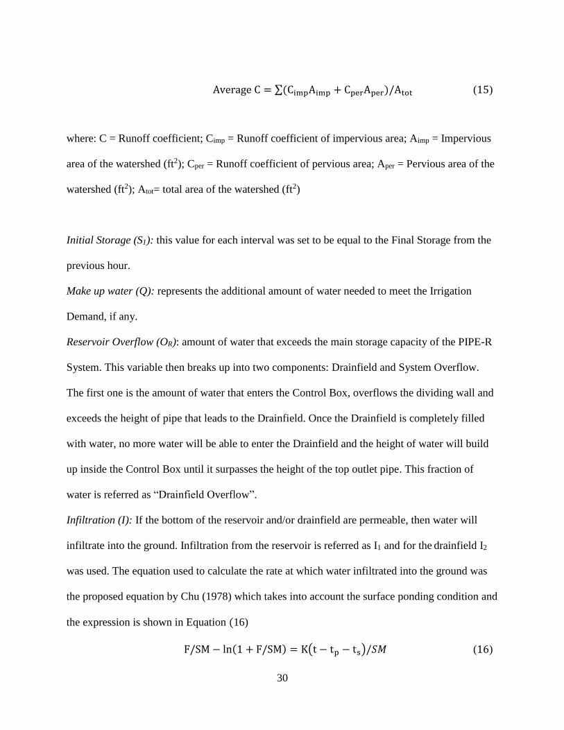
30

Average C = ∑(CimpAimp + CperAper)/Atot (15)

where: C = Runoff coefficient; Cimp = Runoff coefficient of impervious area; Aimp = Impervious

area of the watershed (ft2); Cper = Runoff coefficient of pervious area; Aper = Pervious area of the

watershed (ft2); Atot= total area of the watershed (ft2)

Initial Storage (S1): this value for each interval was set to be equal to the Final Storage from the

previous hour.

Make up water (Q): represents the additional amount of water needed to meet the Irrigation

Demand, if any.

Reservoir Overflow (OR): amount of water that exceeds the main storage capacity of the PIPE-R

System. This variable then breaks up into two components: Drainfield and System Overflow.

The first one is the amount of water that enters the Control Box, overflows the dividing wall and

exceeds the height of pipe that leads to the Drainfield. Once the Drainfield is completely filled

with water, no more water will be able to enter the Drainfield and the height of water will build

up inside the Control Box until it surpasses the height of the top outlet pipe. This fraction of

water is referred as “Drainfield Overflow”.

Infiltration (I): If the bottom of the reservoir and/or drainfield are permeable, then water will

infiltrate into the ground. Infiltration from the reservoir is referred as I1 and for the drainfield I2

was used. The equation used to calculate the rate at which water infiltrated into the ground was

the proposed equation by Chu (1978) which takes into account the surface ponding condition and

the expression is shown in Equation (16)

F/SM − ln(1 + F/SM) = K(t − tp − ts)/𝑆𝑀 (16)

31

In order to produce a highly accurate set of results, additional calculations are needed to

determine if there is surface ponding or not. These calculations consider the amount of storage of

the soil and the amount of water that has been infiltrated, to then produce a value that indicates

whether infiltration will occur at ponded conditions or not. This process was first used in the

PIPE-R Model but caused the program to shut down several times since the amount of data being

analyzed is significantly large. Unsteady state analysis would be beneficial for the simulation of

rainfall events; however, in this case the water is drained to a local underground storage area that

will mostly be ponded. Therefore, a permanent ponded condition was used in the PIPE-R Model

to help the program run smoothly and minimize crashing due to excessive data processing. In

addition, the assumption that the soil infiltrates only in ponded conditions will provide the

system with some margin of error against extreme weather events and slight errors due to

construction. The reason ponded conditions provide safety to the design is because the

infiltration rate is assumed to be slower than when the surface is not ponded, which forces the

design to utilize a bigger volume space for the water to be held. Another assumption related to

infiltration is that no horizontal infiltration occurs, in any direction.

Surface Layer

The upper component is the top layer and its main factor is its permeability, because it

will not let water through unless it is permeable. It can be seen in Figure 8 that the top layer is

affected by how much water is introduced by rainfall (P), the rate at which water evaporates (ET)

and the water available capacity (WAC). The diagram of the surface layer can be seen in Figure

8.

32

Figure 8. Mass balance of top surface layer.

The factors just mentioned help us to determine the rate at which water infiltrates into the

ground. Another soil property that affects infiltration is the water available capacity (WAC),

which describes the ability of soil to hold water typically based on feet of depth. The WAC value

is multiplied by the volume of the layer to predict the storage capacity of the particular layer.

Once the soil reaches the maximum holding capacity, it start releasing the excess water through

the pores, which is referred as “Direct Infiltration” in this study. The WAC for each soil type is

obtained through tables found in literature (Saxton and Rawls 2006).

Other variables needed to complete the mass balance equation for the top surface layer

are precipitation (P) and evapotranspiration (ET). The P values for each 1-hour interval were

obtained from the NOAA website but it was required to make some adjustments to also include

hours were rain did not occur. The ET values are calculated through the equation of Blaney-

Cridell, which evaluates evaporation rates based on a particular latitude, monthly % annual

daytime hours and the crop type. The equation is as follows:

u = ktp/100 (17)

33

The monthly ET coefficient (k) is can be obtained from tables presented in the literature

and they are based on the type of crop where is water is resting on (Maidment 1992). For this

case we have simplified the model and fixed the k to be 0.7 which belongs to grass and the

variables t and p were established based on the location of the system.

Two conditions are considered to determine the magnitude of Direct Infiltration. The first

one occurs when the net amount of water is less than the maximum storage capacity of the layer,

then the value of DI infiltration is zero. The second condition occurs when the net amount of

water is greater than the layer’s storage capacity, which leads the excess water to be infiltrated to

the Reservoir. The equations for the two conditions be seen below (NOTE: All values are based

on unit area).

If: 𝑆1 + 𝑃 − 𝐸𝑇 < 𝑆𝑚𝑎𝑥, 𝑡ℎ𝑒𝑛 𝐷𝐼 = 0 (18)

If: 𝑆1 + 𝑃 − 𝐸𝑇 > 𝑆𝑚𝑎𝑥, 𝑡ℎ𝑒𝑛 𝐷𝐼 = 𝑆1 + 𝑃 − 𝐸𝑇 − 𝑆𝑚𝑎𝑥 (19)

Where: S1 = Initial water storage of the top surface layer (ft); P = Magnitude of

precipitation during the corresponding hourly interval (ft); ET = Evapotranspiration (ft); DI =

Direct Infiltration (ft); Smax = Maximum storage capacity of the top surface layer

Once the location is known, all the factors of the top layer can be determined. A mass

balance equation for the top soil layer is presented as:

dS

dt= P − ET − DI

dS = dt(P − ET − DI)

S2∗ − S1

∗ = dt(P − ET − DI)

34

S2∗ = S1

∗ + P∗ − ET∗ − DI∗ (20)

Drainfield

The Drainfield is an optional additional storage than can be added to the Reservoir. Once

water overflows from the Reservoir (OR) to the Drainfield, it accumulates until its storage

capacity reaches the maximum volume and water cannot enter anymore. At this stage, any

additional water builds up in the Control Box until it overflows to the outside, which is referred

by Drainfield Overflow (OD in Figure 9). NOTE: The volume of the Control Box that

corresponds to this storage was incorporated with the Drainfield, which explains why the control

box is not shown on Figure 9.

Figure 9. System boundary of the Drainfield

Infiltration does occur as long as there is water in the drainfield and its quantification is

done by the Green-Ampt equation. The conditions and equations used to determine the amount

of water in the Drainfield are:

If OR − ID < DS OD = 0 (21)

If OR − ID > Ds OD = OR − ID − DS (22)

where: OR =Reservoir Overflow (ft3); ID = Infiltration from the Drainfield (ft3); DS = Storage

Volume of the Drainfield (ft3); OD = Drainfield Overflow (ft3)

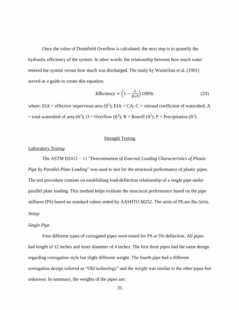
35

Once the value of Drainfield Overflow is calculated, the next step is to quantify the

hydraulic efficiency of the system. In other words, the relationship between how much water

entered the system versus how much was discharged. The study by Wanielista et al. (1991)

served as a guide to create this equation:

Efficiency = (1 −O

R+P) 100% (23)

where: EIA = effective impervious area (ft2); EIA = CA; C = rational coefficient of watershed; A

= total watershed of area (ft2); O = Overflow (ft3); R = Runoff (ft3); P = Precipitation (ft3).

Strength Testing

Laboratory Testing

The ASTM D2412 − 11 “Determination of External Loading Characteristics of Plastic

Pipe by Parallel-Plate Loading” was used to test for the structural performance of plastic pipes.

The test procedure consists on establishing load-deflection relationship of a single pipe under

parallel plate loading. This method helps evaluate the structural performance based on the pipe

stiffness (PS) based on standard values stated by AASHTO M252. The units of PS are lbs./in/in.

Setup

Single Pipe

Four different types of corrugated pipes were tested for PS at 5% deflection. All pipes

had length of 12 inches and inner diameter of 4 inches. The first three pipes had the same design

regarding corrugation style but slight different weight. The fourth pipe had a different

corrugation design referred as “Old technology” and the weight was similar to the other pipes but

unknown. In summary, the weights of the pipes are:

36

1. Pipe #1 - 5.3 oz/ft

2. Pipe #2 - 5.2 oz/ft

3. Pipe #3 - 5.0 oz/ft

4. Pipe #4 - old technology (no assigned weight value)

Equipment needed for the ASTM D2412 – 11 are a testing machine, loading plates and a

deformation indicator. A universal testing machine (UTM) was used for the test and deformed

the pipe at rate of 0.5 in/min as specified in the standard test. Steel plates were required in this

test to help distribute the load evenly on the pipes. The size of the plates met the minimum

parameters stated in the ASTM D2412 – 11. The actual length, width and thickness of the top

plate were 15 in, 8 in and 1 in, respectively. In contrast, a platform of the UTM was used as the

lower plate Figure 10. The deformation indicator was already installed with the UTM. Before the

test, wall thickness and pipe’s lengths measurements are recorded to verify uniformity. The next

step is to place the pipe in the UTM and confirm the contact between the pipe and plate is firm.

A picture of the setup prior to testing can be seen below in and the progression can be seen

below in Figure 10.a. In addition, Figure 10.b-d show progression of the test and illustrates the

deformation experienced by the pipe.

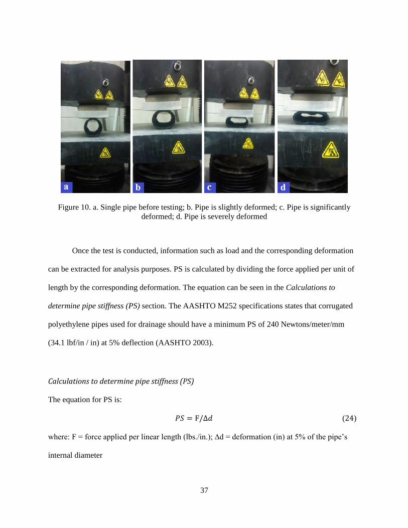
37

Figure 10. a. Single pipe before testing; b. Pipe is slightly deformed; c. Pipe is significantly

deformed; d. Pipe is severely deformed

Once the test is conducted, information such as load and the corresponding deformation

can be extracted for analysis purposes. PS is calculated by dividing the force applied per unit of

length by the corresponding deformation. The equation can be seen in the Calculations to

determine pipe stiffness (PS) section. The AASHTO M252 specifications states that corrugated

polyethylene pipes used for drainage should have a minimum PS of 240 Newtons/meter/mm

(34.1 lbf/in / in) at 5% deflection (AASHTO 2003).

Calculations to determine pipe stiffness (PS)

The equation for PS is:

𝑃𝑆 = F/∆𝑑 (24)

where: F = force applied per linear length (lbs./in.); ∆d = deformation (in) at 5% of the pipe’s

internal diameter

38

Since the inner diameter of the pipe was 4 inches, a 5% vertical deflection of the pipe was

0.2 inches. Consequently, the PS of the pipe was calculated by dividing the load (distributed per

unit length of the pipe) by 0.2 inches. Increasing load was applied to all pipes until the specimens

started deflecting without a load increase. Similarly, another reason to end the test occurred when

the pipe reached failure, defined as experiencing a deflection 30%.

Once the values of the PS for are known for each level, they will be checked against the

minimum requirements specified by AASHTO M252 (34.1 lbf/in/in). The PS stiffness

calculations were designed to analyze a single pipe, but this study also incorporated systems of

bundled pipes. In the original equation the force applied (F) was only divided by the length of the

single pipe. However, the bigger contact area of the system needs to be accounted to more

accurately reflect the load-deflection relationship of the multiple pipes. The proposed changes in

the value of F were to divide the load magnitude by the length of the specimen, but also by the

number pipes in contact with the load.

Another factor to be considered by evaluating multiple pipes under the ASTM D2412 −

11 is the actual height of the pipe system. Since the original PS formula considers the internal

diameter of a pipe, the proposed method consisted of treating the system as single pipe where the

internal diameter was assumed to be the total height of the system minus the pipe’s thickness.

Thus, 5% deflection were based on the new proposed internal diameter. In summary, the

proposed pipe stiffness method for this study accounted for the number of pipes and the height of

the overall pipe bundle system. Further details of the systems are explained in the next section.

𝑃𝑆 = (F/n) /∆ℎ (25)

where: n = number of pipes in contact with loading plate; Δh = deformation (in) at 5% of the

BPU’s overall height.

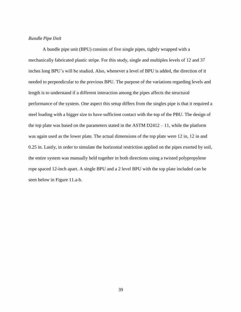
39

Bundle Pipe Unit

A bundle pipe unit (BPU) consists of five single pipes, tightly wrapped with a

mechanically fabricated plastic stripe. For this study, single and multiples levels of 12 and 37

inches long BPU’s will be studied. Also, whenever a level of BPU is added, the direction of it

needed to perpendicular to the previous BPU. The purpose of the variations regarding levels and

length is to understand if a different interaction among the pipes affects the structural

performance of the system. One aspect this setup differs from the singles pipe is that it required a

steel loading with a bigger size to have sufficient contact with the top of the PBU. The design of

the top plate was based on the parameters stated in the ASTM D2412 – 11, while the platform

was again used as the lower plate. The actual dimensions of the top plate were 12 in, 12 in and

0.25 in. Lastly, in order to simulate the horizontal restriction applied on the pipes exerted by soil,

the entire system was manually held together in both directions using a twisted polypropylene

rope spaced 12-inch apart. A single BPU and a 2 level BPU with the top plate included can be

seen below in Figure 11.a-b.

40

Figure 11.a. Single BPU before testing; b. Two-Level BPU before testing with top plate

According to the ASTM D2412 – 11, failure point was reached when a pipe experienced

a deformation that is equal in magnitude to 30% of the pipe’s inside diameter. Since this study

deals with multiple pipes, the maximum allowable deformation was based on the height of the

bundle minus the pipe’s wall thickness. Once the maximum allowable deformation was

established by multiplying the height of the bundle minus the pipe’s wall thickness by 30%, 10

intermediate deflections intervals were selected at which measurements were taken from

particular sections of the pipes. The purpose of the intermediate measurements were to have a

better understanding on how the pipe behaves during testing.

The setup for the 37 in. long BPU had similarities and differences compared the testing of

12 in. long BPU. The concept of establishing load-deflection relationship of the pipes under

parallel plate loading is still the focus but calculations will change. The variations will be

41

explained in the Calculations to determine pipe stiffness (PS). The rate of load application was

also 0.5 in/min and the method of obtaining measurements through the laser position sensor was

also used. However, among some of the main differences are that three BPU’s are used in each

level, bigger top and bottom steel plates are required and the use of a different testing machine

that did not have a deformation indicator. The size of the plates were increased to satisfy the

parameters stated in the ASTM D2412 – 11. The length, width and thickness of the plates were

38 in., 38 in. and 0.25 in. respectively. In addition, steel toes were added to the perimeter of the

plates to reduce bending during loading (See Figure 12 and Figure 13). To resolve the issue of

not being able to automatically obtain load-deflection values through the testing machine,

measurements were taken exclusively with laser position sensor and matched with the load

values shown by the testing machine output window.

Figure 12. One level system of the 37 in. long BPU’s

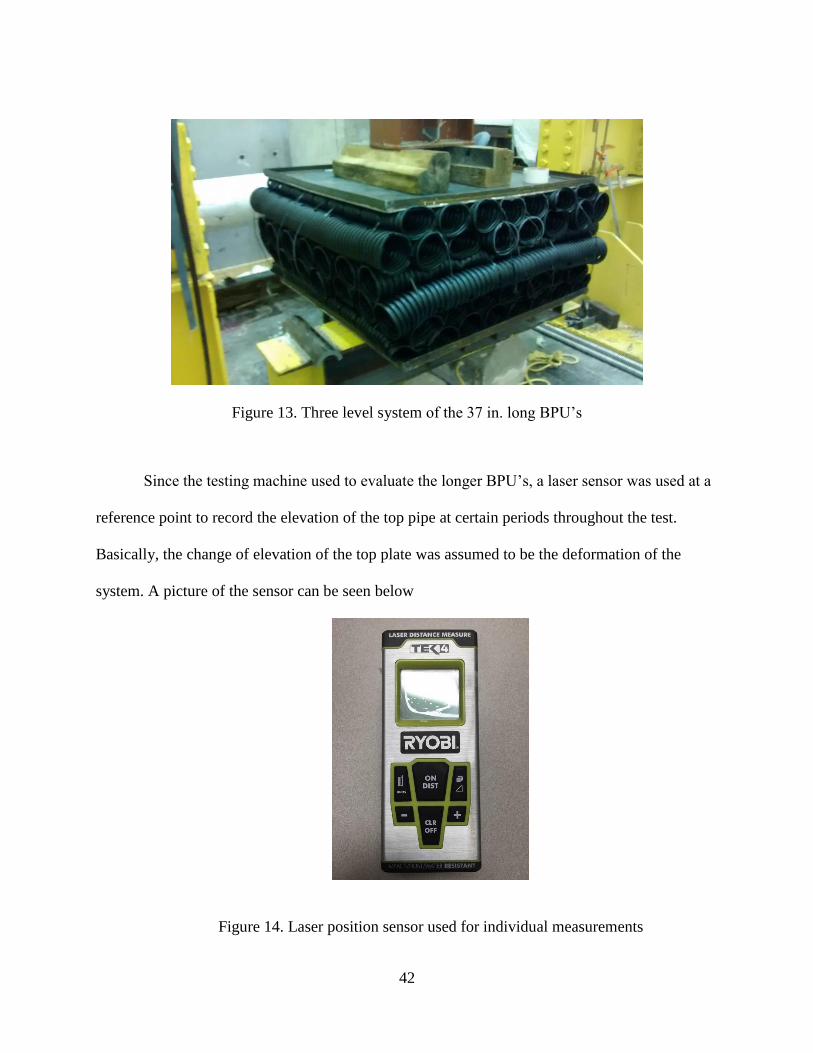
42

Figure 13. Three level system of the 37 in. long BPU’s

Since the testing machine used to evaluate the longer BPU’s, a laser sensor was used at a

reference point to record the elevation of the top pipe at certain periods throughout the test.

Basically, the change of elevation of the top plate was assumed to be the deformation of the

system. A picture of the sensor can be seen below

Figure 14. Laser position sensor used for individual measurements

43

The laser sensor measures the distance until the next object in the direction it is directed,

in this case the object was the bottom of the top plate. A long aluminum ruler and flat steel bar

were used to mark the exact point and create a surface where the laser position sensor could

obtain a measurement. A level was used to verify the tools were exactly horizontal and obtain

more accurate values. An illustration of the setup can be seen in Figure 15

BC

Top

pipe

Lower plate

goes down

Reference Point

Measurement

taken

Figure 15. Setup for individual measurements

Field Testing

Field testing was also conducted to study the structural integrity of the pipe bundles in the

field under the effect of dead, live loads and the addition of pipe-soil interaction. Three systems

of pipe bundles were buried under different cover depths, which will be illustrated later in this

section. Loads applied to the systems were produced by the earth pressure and by vehicular load.

The dimensions testing site were designed to accommodate three 20 ft by 10ft pipe bundle

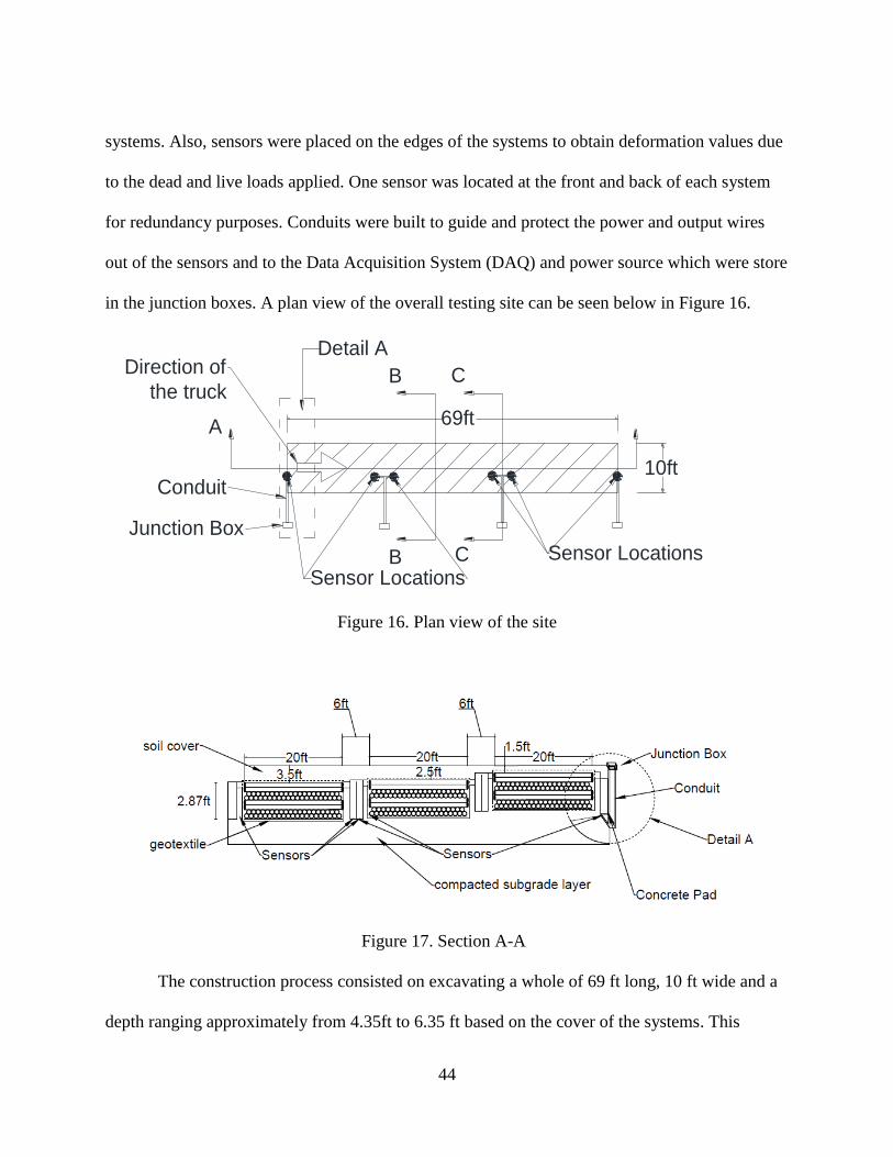
44

systems. Also, sensors were placed on the edges of the systems to obtain deformation values due

to the dead and live loads applied. One sensor was located at the front and back of each system

for redundancy purposes. Conduits were built to guide and protect the power and output wires

out of the sensors and to the Data Acquisition System (DAQ) and power source which were store

in the junction boxes. A plan view of the overall testing site can be seen below in Figure 16.

69ft

10ft

Junction Box

Direction of

the truck

Conduit

B

B

C

C

A

Sensor Locations

Detail A

Sensor Locations

Figure 16. Plan view of the site

Figure 17. Section A-A

The construction process consisted on excavating a whole of 69 ft long, 10 ft wide and a

depth ranging approximately from 4.35ft to 6.35 ft based on the cover of the systems. This

45

difference in height lead to creation of steps in the surface of the excavation (See Figure 18.a).

Once excavation process was over, compaction effort was conducted on the soil surface using a

vibratory plate (See Figure 18.b). Next, the systems were put in place along with the geotextile

which was customized based on the system dimensions. Additionally, structures located next to

the system served as housing for the sensors (See Figure 18.c). After the system had been set in

place, layers of sand, #57 stone and milling were placed according to the particular cover

configuration for each system (details can be found in the Setup dimensions section). Also, PVC

pipes were used as conduits for sensor wires. The finished testing site can be seen in Figure 18.d.

Figure 18.a. Excavated holes; b. Vibratory machine used for compaction; c. System being put

into the holes; d. View of finished testing site

a

.

b

.

c

.

d

.

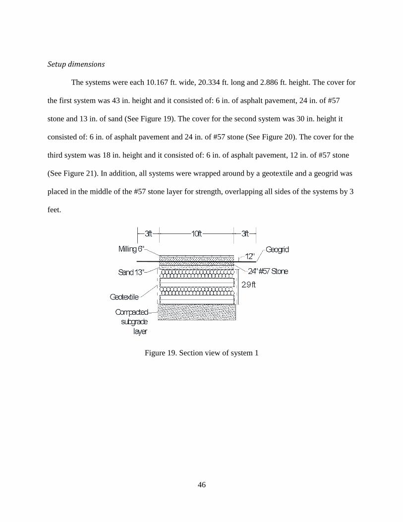
46

Setup dimensions

The systems were each 10.167 ft. wide, 20.334 ft. long and 2.886 ft. height. The cover for

the first system was 43 in. height and it consisted of: 6 in. of asphalt pavement, 24 in. of #57

stone and 13 in. of sand (See Figure 19). The cover for the second system was 30 in. height it

consisted of: 6 in. of asphalt pavement and 24 in. of #57 stone (See Figure 20). The cover for the

third system was 18 in. height and it consisted of: 6 in. of asphalt pavement, 12 in. of #57 stone

(See Figure 21). In addition, all systems were wrapped around by a geotextile and a geogrid was

placed in the middle of the #57 stone layer for strength, overlapping all sides of the systems by 3

feet.

Figure 19. Section view of system 1

47



Sensors were protected by a concrete structure and fixed to a cinder block that was placed

at the bottom of the structure. The mechanism used to record the deflection in the systems was

connecting the sensor’s wire to a metal bar, which was secured to the top level of the system’s

top pipe (See Figure 22).

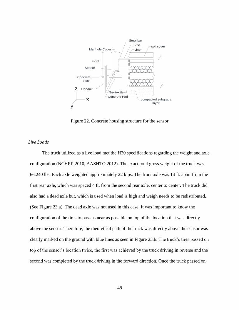
48

z

Sensor

x

Liner

y

4-6 ft

Conduit

compacted subgrade

layer

soil cover

Concrete Pad

Geotextile

12"Ø

Manhole Cover

Steel bar

Concrete

block

Figure 22. Concrete housing structure for the sensor

Live Loads

The truck utilized as a live load met the H20 specifications regarding the weight and axle

configuration (NCHRP 2010, AASHTO 2012). The exact total gross weight of the truck was

66,240 lbs. Each axle weighted approximately 22 kips. The front axle was 14 ft. apart from the

first rear axle, which was spaced 4 ft. from the second rear axle, center to center. The truck did

also had a dead axle but, which is used when load is high and weigh needs to be redistributed.

(See Figure 23.a). The dead axle was not used in this case. It was important to know the

configuration of the tires to pass as near as possible on top of the location that was directly

above the sensor. Therefore, the theoretical path of the truck was directly above the sensor was

clearly marked on the ground with blue lines as seen in Figure 23.b. The truck’s tires passed on

top of the sensor’s location twice, the first was achieved by the truck driving in reverse and the

second was completed by the truck driving in the forward direction. Once the truck passed on

49

top of the sensor twice, the truck drove away a small distance such 10 feet and then repeated the

operation Figure 23.c. Pictures from the truck can be seen below:

Figure 23.a. 2 rear axles and a dead axle; b. Two rear axles following the blue lines; c. Rear view

of the truck driving away from the sensor’s location

While the truck was in motion, draw-wire sensors were utilized to measure the deflection

experience in each system. The location of the measuring devices are on both edges of the

systems, directly underneath of the path of the truck’s tires (See Figure 24).

10ft

Cover varies 18"-43"

Compacted

subgrade

layerSensor

2ftdual wheel

Geotextile

Figure 24. Location of tires with respect to sensor

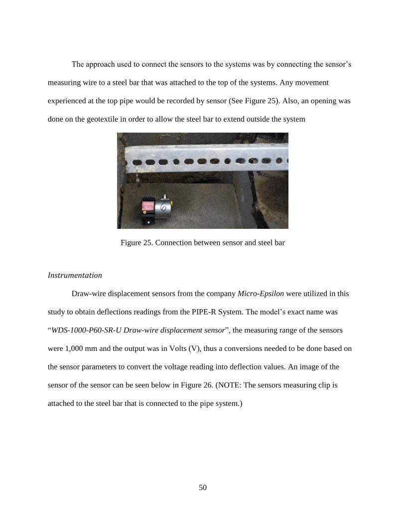
50

The approach used to connect the sensors to the systems was by connecting the sensor’s

measuring wire to a steel bar that was attached to the top of the systems. Any movement

experienced at the top pipe would be recorded by sensor (See Figure 25). Also, an opening was

done on the geotextile in order to allow the steel bar to extend outside the system

Figure 25. Connection between sensor and steel bar

Instrumentation

Draw-wire displacement sensors from the company Micro-Epsilon were utilized in this

study to obtain deflections readings from the PIPE-R System. The model’s exact name was

“WDS-1000-P60-SR-U Draw-wire displacement sensor”, the measuring range of the sensors

were 1,000 mm and the output was in Volts (V), thus a conversions needed to be done based on

the sensor parameters to convert the voltage reading into deflection values. An image of the

sensor of the sensor can be seen below in Figure 26. (NOTE: The sensors measuring clip is

attached to the steel bar that is connected to the pipe system.)

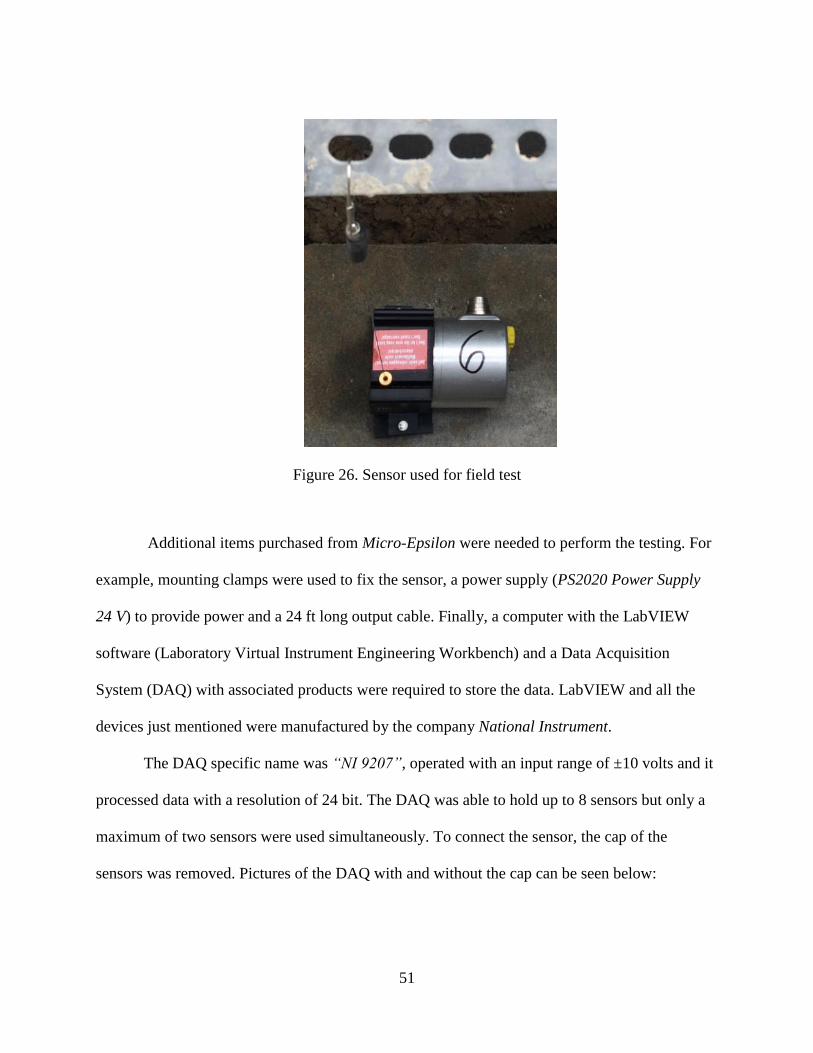
51

Figure 26. Sensor used for field test

Additional items purchased from Micro-Epsilon were needed to perform the testing. For

example, mounting clamps were used to fix the sensor, a power supply (PS2020 Power Supply

24 V) to provide power and a 24 ft long output cable. Finally, a computer with the LabVIEW

software (Laboratory Virtual Instrument Engineering Workbench) and a Data Acquisition

System (DAQ) with associated products were required to store the data. LabVIEW and all the

devices just mentioned were manufactured by the company National Instrument.

The DAQ specific name was “NI 9207”, operated with an input range of ±10 volts and it

processed data with a resolution of 24 bit. The DAQ was able to hold up to 8 sensors but only a

maximum of two sensors were used simultaneously. To connect the sensor, the cap of the

sensors was removed. Pictures of the DAQ with and without the cap can be seen below:

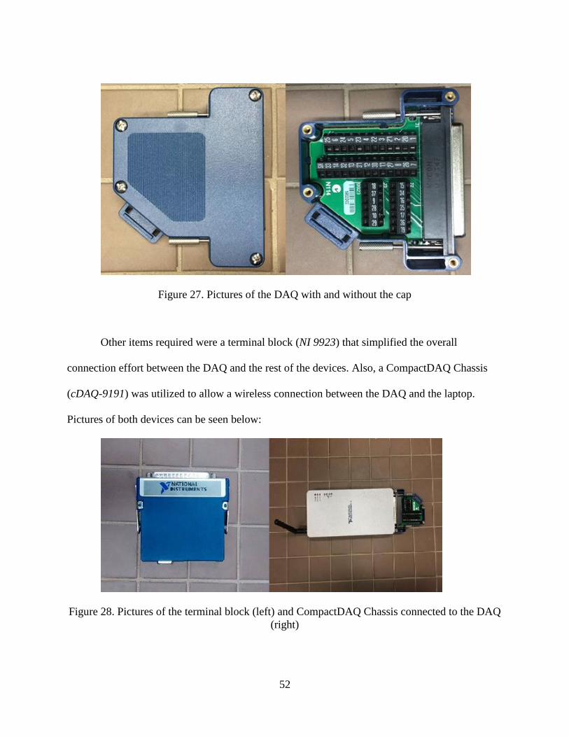
52

Figure 27. Pictures of the DAQ with and without the cap

Other items required were a terminal block (NI 9923) that simplified the overall

connection effort between the DAQ and the rest of the devices. Also, a CompactDAQ Chassis

(cDAQ-9191) was utilized to allow a wireless connection between the DAQ and the laptop.

Pictures of both devices can be seen below:

Figure 28. Pictures of the terminal block (left) and CompactDAQ Chassis connected to the DAQ

(right)

53

Finally, the last product was a power supply with the specific name of Power Cord, AC,

U.S., 120 VAC, 2.3 meters. The power supply was connected directly to the DAQ and it was

used to power the system. A picture of the power supply can be seen below:

Figure 29. Power supply

LabVIEW is computer software that allows visual programming through the language

“G”. A bug in the LabVIEW was found while activating the devices, thus a particular system

configuration was designed manually in LabVIEW to obtain the data, convert it to a readable

format and save it properly. The diagram to allow the proper reading from the sensors can be

seen below in Figure 30:

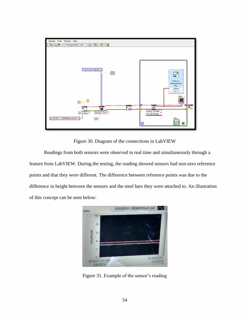
54

Figure 30. Diagram of the connections in LabVIEW

Readings from both sensors were observed in real time and simultaneously through a

feature from LabVIEW. During the testing, the reading showed sensors had non-zero reference

points and that they were different. The difference between reference points was due to the

difference in height between the sensors and the steel bars they were attached to. An illustration

of this concept can be seen below:

Figure 31. Example of the sensor’s reading

55

Since the sensors were located underground, the output wires were a concern of the

design. The solution to this problem was to use PVC pipes to guide and protect the wires from

the sensor to the DAQ (See Figure 32).

Sensor

Concrete Pad

soil surface

Conduit

DAQ Laptop w/

Labview

Figure 32. Conduit from housing structure to DAQ

56

CHAPTER 4: RESULTS

PIPE-R Model: Example Problem

Part A

The PIPE-R model was used for a project located in Orlando, Florida having a watershed

area have of 110,000 ft2 and 80,000 ft2 of it was impervious. Default values and the auto

calculated weighted runoff coefficient were utilized to determine runoff. The target efficiency

was a minimum of 80%.

The desired width, length and height of the reservoir were 35 ft, 30 ft and 4 ft,

respectively. The soil type underneath the reservoir was “Sand”. Default values were used to

determine the soil properties of interest. The infiltration rate was determined from this data. The

surface layer above the system was 24 inches of “Sand”. Again, default values were used to

determine storage and infiltration values required to run the model. Both the top surface layer

above the reservoir and the bottom of the reservoir were permeable. This system was an

underground exfiltration system, e.g. no water demand were used for this part of the problem.

Procedure:

1. Model was opened.

2. Macros are enabled

3. The manual calculation feature, located under the formulas tab, was selected (See Figure

33).

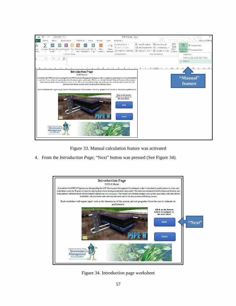
57

Figure 33. Manual calculation feature was activated

4. From the Introduction Page, “Next” button was pressed (See Figure 34).

Figure 34. Introduction page worksheet

“Manual”

feature

“Next”

58

5. From the General Instruction worksheet (See Figure 35), the “Next” button was pressed

to proceed to the NOAA Website Instructions worksheet.

Figure 35. General Instructions worksheet

6. From the NOAA Website Instructions worksheet, the next steps were followed (See

Figure 36).

a. The following link was copied and pasted in a browser

http://www.ncdc.noaa.gov/cdo-web/search?datasetid=PRECIP_HLY

Figure 36: Instructions to obtain historical data from NOAA

b. The “Precipitation Hourly” option was selected as the weather observation type.

(See Figure 37)

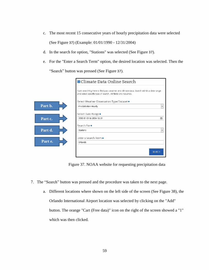
http://www.ncdc.noaa.gov/cdo-web/search?datasetid=PRECIP_HLY

59

c. The most recent 15 consecutive years of hourly precipitation data were selected

(See Figure 37) (Example: 01/01/1990 - 12/31/2004)

d. In the search for option, "Stations" was selected (See Figure 37).

e. For the "Enter a Search Term" option, the desired location was selected. Then the

“Search” button was pressed (See Figure 37).

Figure 37. NOAA website for requesting precipitation data

7. The “Search” button was pressed and the procedure was taken to the next page.

a. Different locations where shown on the left side of the screen (See Figure 38), the

Orlando International Airport location was selected by clicking on the "Add"

button. The orange "Cart (Free data)" icon on the right of the screen showed a "1"

which was then clicked.

Part b.

Part c.

Part e.

Part d.

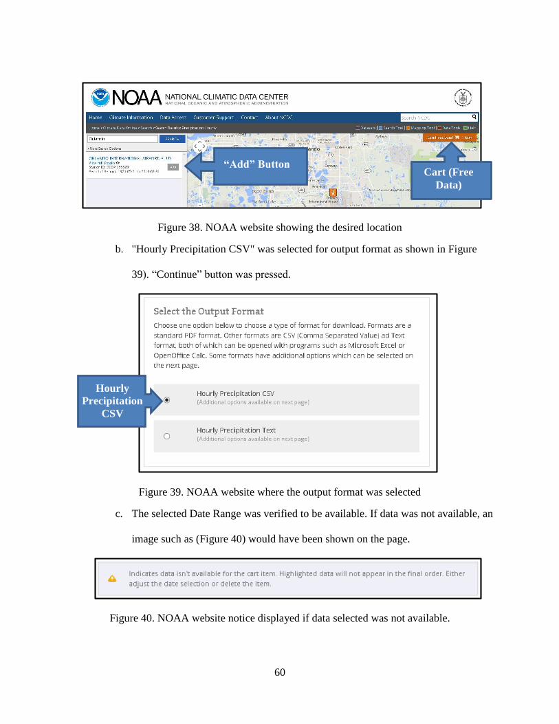
60

Figure 38. NOAA website showing the desired location

b. "Hourly Precipitation CSV" was selected for output format as shown in Figure

39). “Continue” button was pressed.

Figure 39. NOAA website where the output format was selected

c. The selected Date Range was verified to be available. If data was not available, an

image such as (Figure 40) would have been shown on the page.

Figure 40. NOAA website notice displayed if data selected was not available.

“Add” Button Cart (Free

Data)

Hourly

Precipitation

CSV

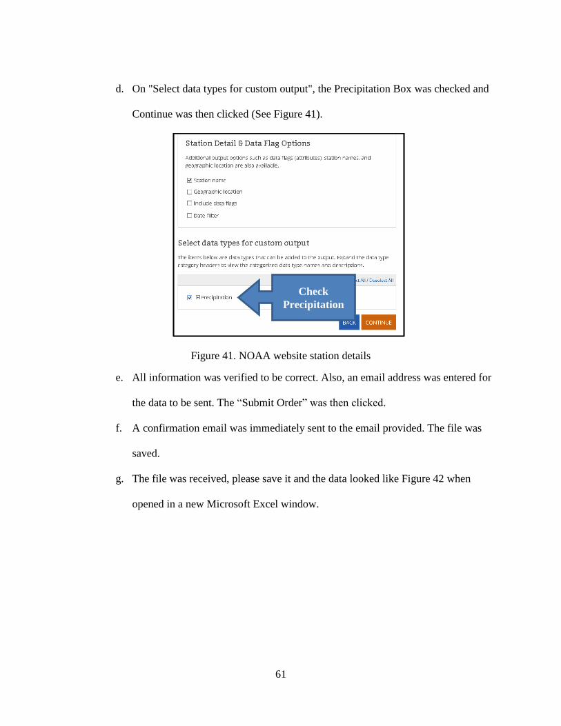
61

d. On "Select data types for custom output", the Precipitation Box was checked and

Continue was then clicked (See Figure 41).

Figure 41. NOAA website station details

e. All information was verified to be correct. Also, an email address was entered for

the data to be sent. The “Submit Order” was then clicked.

f. A confirmation email was immediately sent to the email provided. The file was

saved.

g. The file was received, please save it and the data looked like Figure 42 when

opened in a new Microsoft Excel window.

Check

Precipitation

62

Figure 42. Example of precipitation data

8. The file with the precipitation data was imported into the PIPE-R model

a. Import Data was clicked (See Figure 44). A message with a question asked

whether to proceed or not, “Yes” was clicked.

Figure 43. Empty Historical Data worksheet

Import Data

button

63

b. A browser opened (See Figure 44), the previously saved file with precipitation of

the city of Orlando was selected. Note: It took a minute to download.

Figure 44. Browse for file

c. Once opened, the Historical Data worksheet looked like Figure 45.

Figure 45. Example of imported data

d. When the data was done uploading, “Next” was clicked and the model proceeded

to the Site Characteristics worksheet.

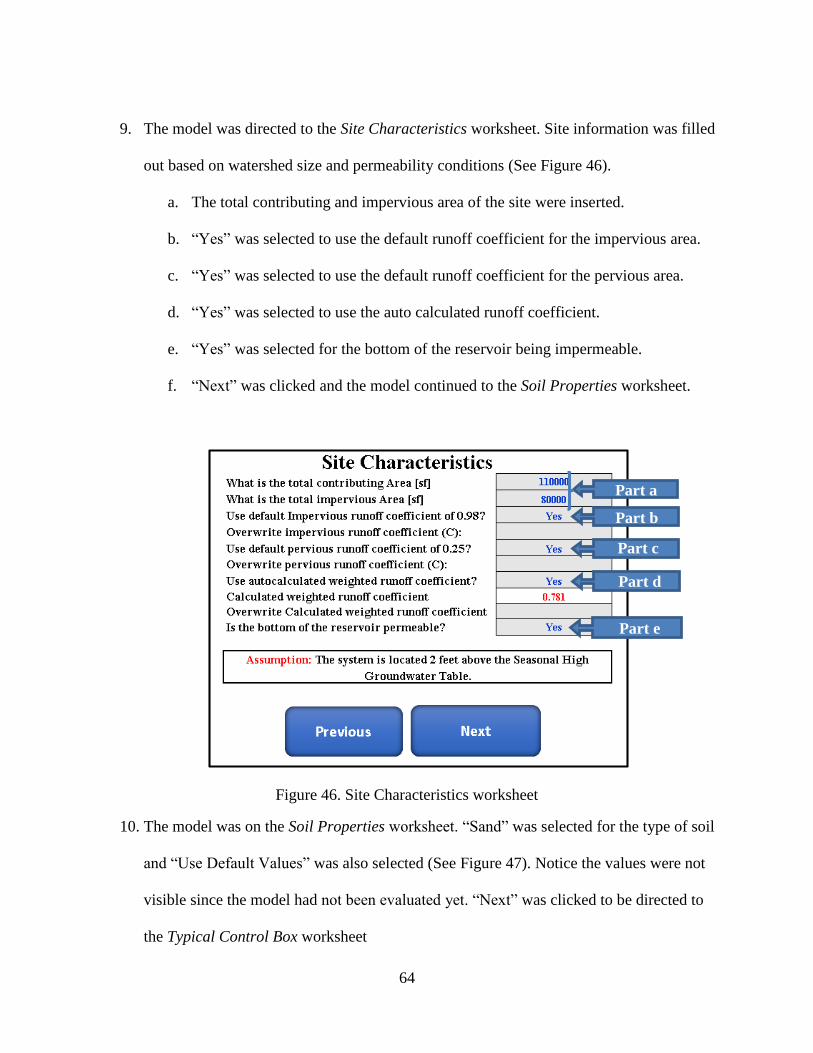
64

9. The model was directed to the Site Characteristics worksheet. Site information was filled

out based on watershed size and permeability conditions (See Figure 46).

a. The total contributing and impervious area of the site were inserted.

b. “Yes” was selected to use the default runoff coefficient for the impervious area.

c. “Yes” was selected to use the default runoff coefficient for the pervious area.

d. “Yes” was selected to use the auto calculated runoff coefficient.

e. “Yes” was selected for the bottom of the reservoir being impermeable.

f. “Next” was clicked and the model continued to the Soil Properties worksheet.

Figure 46. Site Characteristics worksheet

10. The model was on the Soil Properties worksheet. “Sand” was selected for the type of soil

and “Use Default Values” was also selected (See Figure 47). Notice the values were not

visible since the model had not been evaluated yet. “Next” was clicked to be directed to

the Typical Control Box worksheet

Part a

Part b

Part c

Part d

Part e

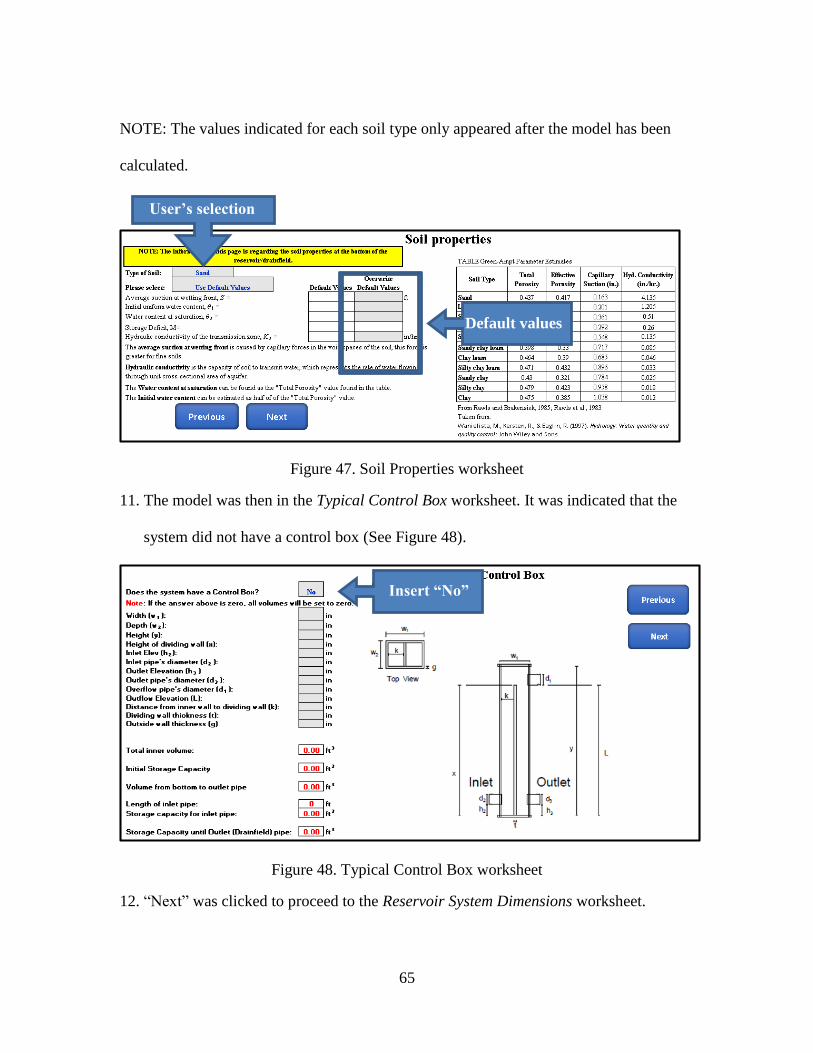
65

NOTE: The values indicated for each soil type only appeared after the model has been

calculated.

Figure 47. Soil Properties worksheet

11. The model was then in the Typical Control Box worksheet. It was indicated that the

system did not have a control box (See Figure 48).

Figure 48. Typical Control Box worksheet

12. “Next” was clicked to proceed to the Reservoir System Dimensions worksheet.

User’s selection

Default values

Insert “No”

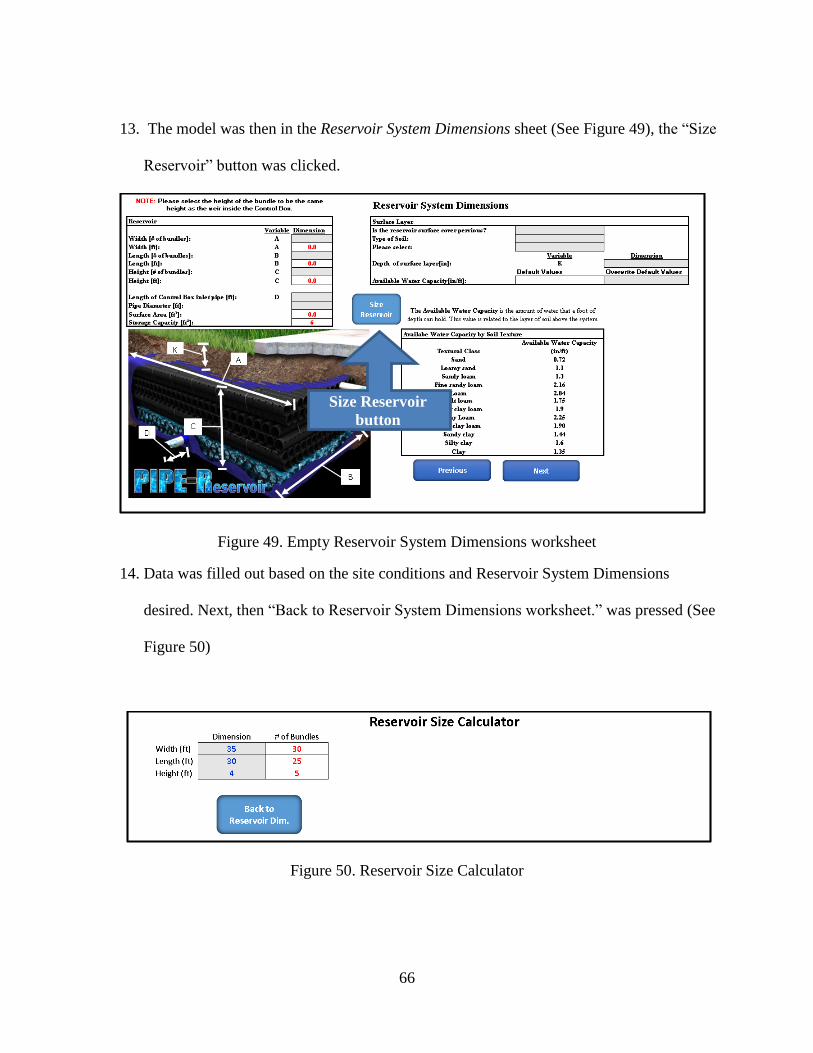
66

13. The model was then in the Reservoir System Dimensions sheet (See Figure 49), the “Size

Reservoir” button was clicked.

Figure 49. Empty Reservoir System Dimensions worksheet

14. Data was filled out based on the site conditions and Reservoir System Dimensions

desired. Next, then “Back to Reservoir System Dimensions worksheet.” was pressed (See

Figure 50)

Figure 50. Reservoir Size Calculator

Size Reservoir

button

67

15. In the Reservoir System Dimensions worksheet, the information was filled out according

to the values information given in the problem statement as shown in

Figure 51. “Next” was clicked to proceed to the Drainfield worksheet.

Figure 51. Reservoir System Dimensions worksheet

Fill out

information

68

16. The model was then on the Drainfield worksheet. It was indicated that the system did not

have a drainfield (See Figure 52). “Next” was clicked to proceed to the Irrigation

Demand worksheet.

Figure 52. Drainfield worksheet

17. The model was then on the Irrigation Demand worksheet. Since no water demand was

specified in the problem statement, Florida was simply selected from the drop down

menu (See Figure 53). “Next” was clicked to continue to the Grey Water Demand

worksheet.

Insert “No”

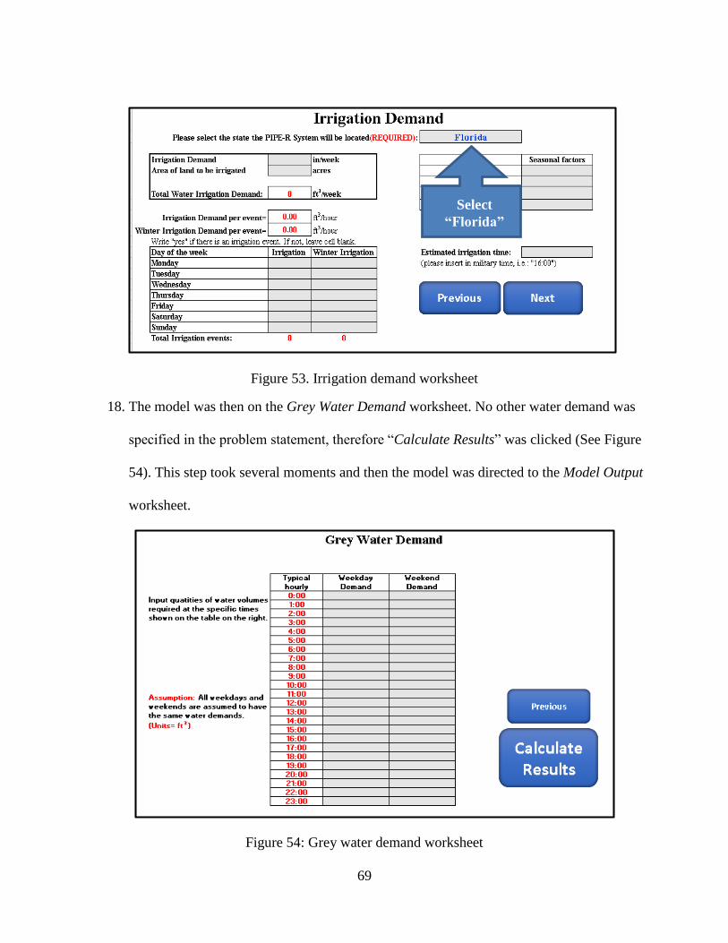
69

Figure 53. Irrigation demand worksheet

18. The model was then on the Grey Water Demand worksheet. No other water demand was

specified in the problem statement, therefore “Calculate Results” was clicked (See Figure

54). This step took several moments and then the model was directed to the Model Output

worksheet.

Figure 54: Grey water demand worksheet

Select

“Florida”

70

19. The model was then on the Model Output worksheet. The Model Output worksheet

showed a summary of the relevant information about the PIPE-R system modeled. The

average yearly rainfall for the project location was presented, along with the average

yearly hydrologic efficiency and the average yearly groundwater recharge. The

dimensions of the system were also summarized for convenience. Since the hydraulic

efficiency was less than 80% some changes were made to the model (See Figure 55).

Figure 55. Model Output worksheet

Part B

Part A of this example did not achieve the desired 80% average yearly hydrologic

efficiency. To meet this objective, a few changes were made to the system in order to achieve the

desired results. A drainfield, along with a control box, were added to the system. Additionally,

water was harvested from the system to meet certain demands.

The length of the pipes from the reservoir to the control box was 4 ft and the pipe’s inside

diameter was 4 in. (0.33 ft). The length of the pipes from the control box to the drainfield were

71

10.5 ft and have an inside diameter of 4 in (0.33 ft). The length, width and height of the

drainfield were 50 ft, 50 ft, and 4 ft, respectively. The amount of linear feet of pipes in the

drainfield was 150 LF and the porosity of the filler stone was 0.3.

An irrigation demand were added with seasonal factors for each season as follows: 1.25

(Summer), 1.00 (Fall), 0.75 (Winter), 1.00 (Spring). The irrigation demand was 1 in/week and

the irrigated area was 1 acre. There were 2 irrigation schedules, the main one consisted of 3

irrigation events per week which were at 4:00 AM on Monday, Wednesday and Friday. The

second was for winter season and consisted of 2 irrigation events per week which were at 4:00

AM on Tuesday and Thursday.

The width, depth and height of the control box were 24 in, 24 in and 108 in, respectively.

The height of the weir inside the control box was 43.2 in and the thickness of that weir wall was

1 in. The height of the bottom of the inlet pipe was 12 in and had an inside diameter of 4 in. The

outlet pipe directing water to the drainfield had the same two dimensions. The elevation for the

bottom of the overflow pipe had an elevation of 90 in and its internal diameter was also 4 in. The

thickness of the outside walls was 1 in and the distance between the inner wall and the side of the

inlet pipe was 11.5 in.

Procedure:

To make changes, the button “Return to Start Page” was clicked to navigate to the Site

Characteristics worksheet. Since a drainfield was added, the bottom of the reservoir was

changed to impermeable.

1. The model was then in the Site Characteristics worksheet. “No” was selected to indicate

the bottom of the reservoir was impermeable (See Figure 56).

72

Figure 56. Site Characteristics worksheet

2. “Next” was pressed to continue to the Soil properties worksheet.

3. No changes needed to be made in the Soil properties sheet. “Next” was clicked to

continue to the Typical Control Box worksheet.

4. In the Typical Control Box worksheet, it was indicated the system did have a control box

(See Figure 57), all required dimensions were filled out based on the statement on Part B.

“Next” was clicked to proceed to the next worksheet.

Select “No”

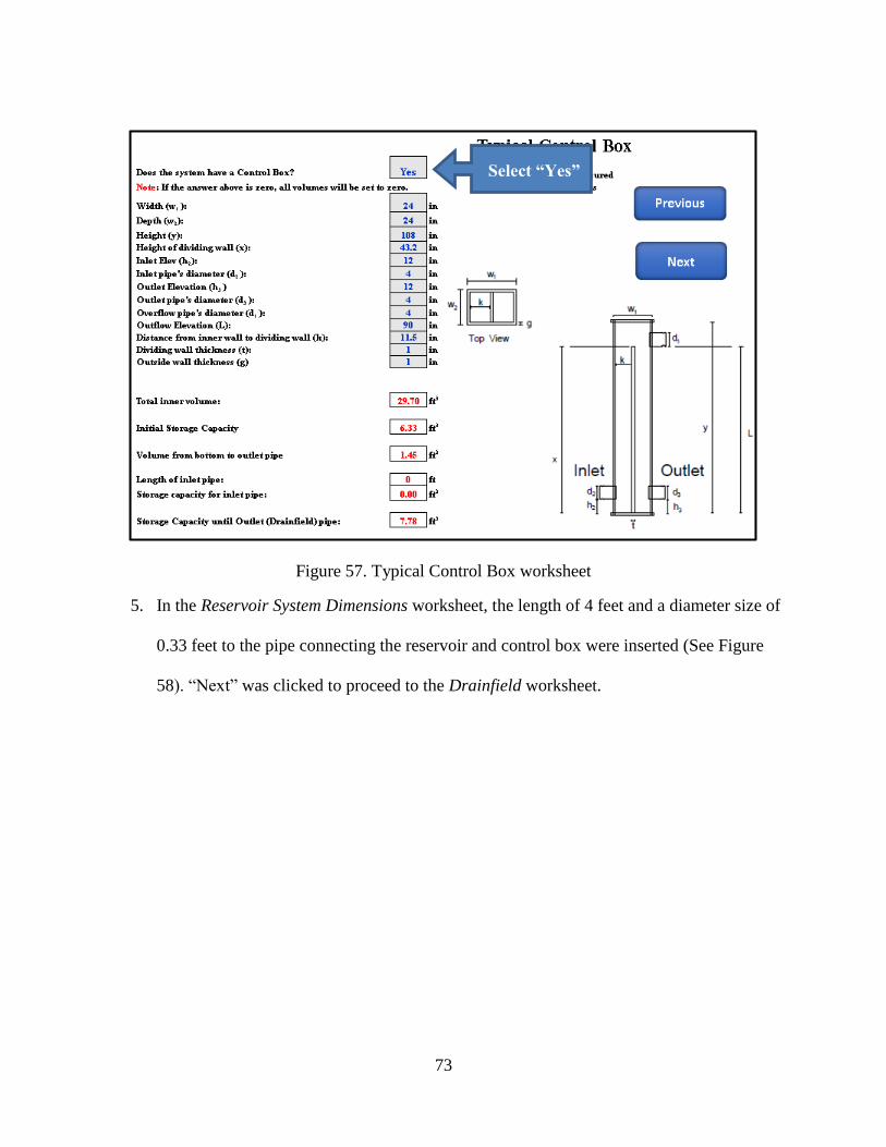
73

Figure 57. Typical Control Box worksheet

5. In the Reservoir System Dimensions worksheet, the length of 4 feet and a diameter size of

0.33 feet to the pipe connecting the reservoir and control box were inserted (See Figure

58). “Next” was clicked to proceed to the Drainfield worksheet.

Select “Yes”

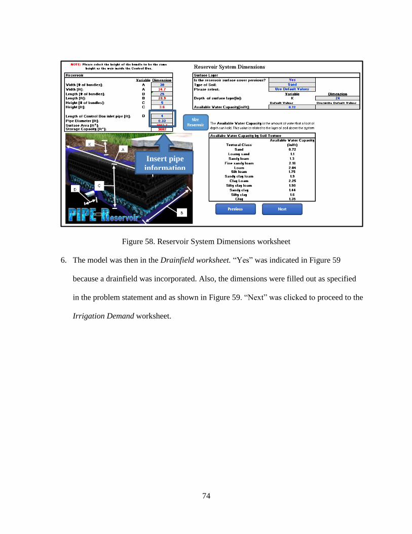
74

Figure 58. Reservoir System Dimensions worksheet

6. The model was then in the Drainfield worksheet. “Yes” was indicated in Figure 59

because a drainfield was incorporated. Also, the dimensions were filled out as specified

in the problem statement and as shown in Figure 59. “Next” was clicked to proceed to the

Irrigation Demand worksheet.

Insert pipe

information

75

Figure 59. Drainfield worksheet

7. In the Irrigation Demand worksheet, the irrigation demand data was specified based the

dimensions desired in Part B (See Figure 60).

Figure 60. Irrigation demand worksheet

Select “Yes”

Intensity

and area

Seasonal

factors

Time

Schedule

76

8. The model was then in the Grey Water Demand worksheet, no grey water demands were

specified in the statement of Part B.

Figure 61. Grey Water Demand worksheet

9. “Calculate Results” button was pressed to proceed to the Model Output worksheet.

In the Model Output worksheet, the average yearly rainfall for the project location was again

presented, along with the average yearly hydrologic efficiency and the average yearly

groundwater recharge. The dimensions of the system were also summarized for convenience.

Since the hydraulic efficiency was above 80%, the performance criteria had been met

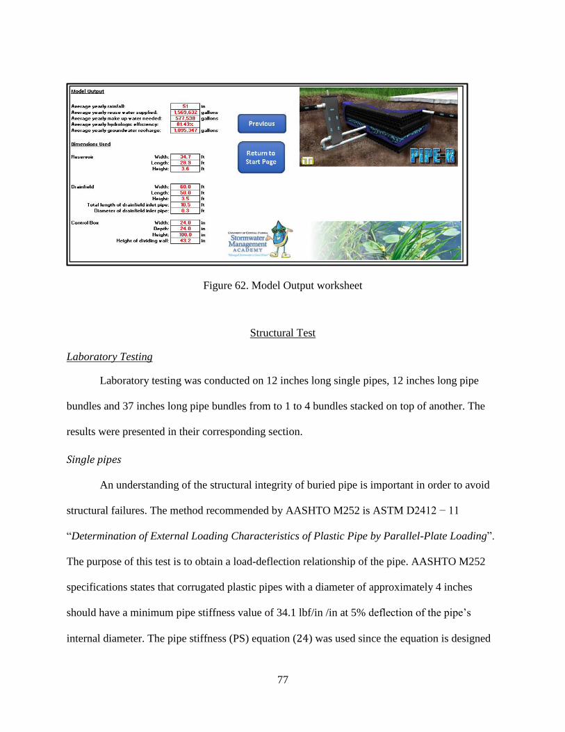
77

Figure 62. Model Output worksheet

Structural Test

Laboratory Testing

Laboratory testing was conducted on 12 inches long single pipes, 12 inches long pipe

bundles and 37 inches long pipe bundles from to 1 to 4 bundles stacked on top of another. The

results were presented in their corresponding section.

Single pipes

An understanding of the structural integrity of buried pipe is important in order to avoid

structural failures. The method recommended by AASHTO M252 is ASTM D2412 − 11

“Determination of External Loading Characteristics of Plastic Pipe by Parallel-Plate Loading”.

The purpose of this test is to obtain a load-deflection relationship of the pipe. AASHTO M252

specifications states that corrugated plastic pipes with a diameter of approximately 4 inches

should have a minimum pipe stiffness value of 34.1 lbf/in /in at 5% deflection of the pipe’s

internal diameter. The pipe stiffness (PS) equation (24) was used since the equation is designed

78

to evaluate single pipes and this approach will be referred as PS 1 in tables throughout this

document. The table below shows the pipe stiffness (PS) values for each type of pipe:

Table 1: Summary of PS for single pipes

Pipe #1

(5.3

oz/ft)

PS 1

(lbf/in/in)

Pipe #2

(5.2

oz/ft)

PS 1

(lbf/in/in)

Pipe #3

(5.0

oz/ft)

PS 1

(lbf/in/in)

Pipe

#4

(old

tech.)

PS 1

(lbf/in/in)

1A 51.42 2A 38.78 3A 48.47 4A 54.39

1B 34.86 2B 34.54 3B 54.97 4B 54.30

1C 49.20 2C 56.97 3C 35.86 4C 54.68

1D 55.21 4D 56.28

1E 59.41 4E 47.80

4F 53.94

Mean 50.02 Mean 43.43 Mean 46.43 Mean 53.49

It was observed in Table 1 that individual and averaged PS values for all pipes exceeded

the minimum value stated by AASHTO M252 (34.1 lbf/in/in). The average PS values for the

four different type of pipes exceeded the requirement by a range of 27% to 56%. It can also be

determined that Pipe #4 (Old technology) performed better than the other three pipes. The

manufacturer of the pipe expressed that pipes #1, #2 and #3 had not been subjected to quality

standards and that they were fabricated with a different mixture. The lack of quality testing and

different mixture might be a reason why pipe #4 showed greater strength.

The pipes also showed significant ability to rebound after a few minutes of been

compressed fully. This behavior is typical from this material is caused due to the molecular

properties (Kissin 2012). Kissin (2012) explained that polymer have fewer crystalline areas than

rigid objects in their chemical composition, which allow greater movement of atoms and provide

flexibility to the material. During the loading procedure, the pipe did not show signs of rupture

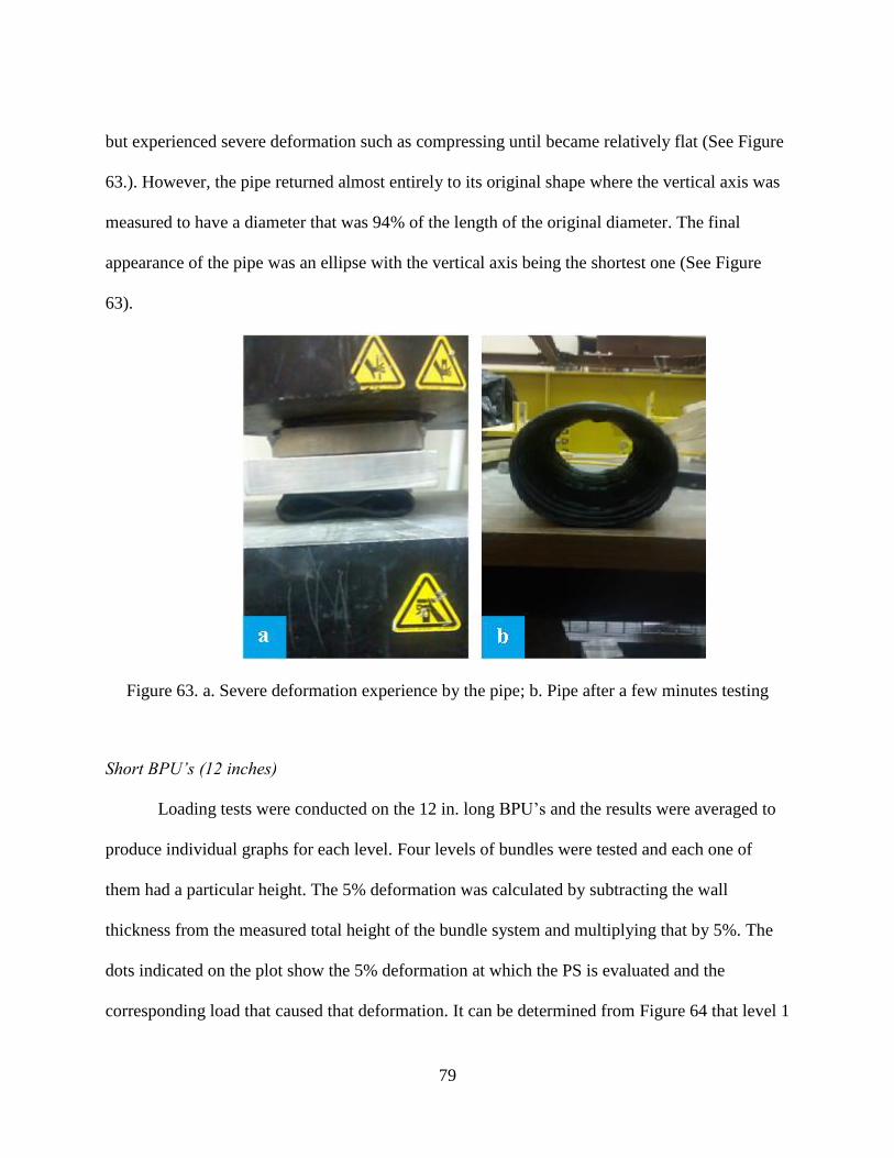
79

but experienced severe deformation such as compressing until became relatively flat (See Figure

63.). However, the pipe returned almost entirely to its original shape where the vertical axis was

measured to have a diameter that was 94% of the length of the original diameter. The final

appearance of the pipe was an ellipse with the vertical axis being the shortest one (See Figure

63).

Figure 63. a. Severe deformation experience by the pipe; b. Pipe after a few minutes testing

Short BPU’s (12 inches)

Loading tests were conducted on the 12 in. long BPU’s and the results were averaged to

produce individual graphs for each level. Four levels of bundles were tested and each one of

them had a particular height. The 5% deformation was calculated by subtracting the wall

thickness from the measured total height of the bundle system and multiplying that by 5%. The

dots indicated on the plot show the 5% deformation at which the PS is evaluated and the

corresponding load that caused that deformation. It can be determined from Figure 64 that level 1

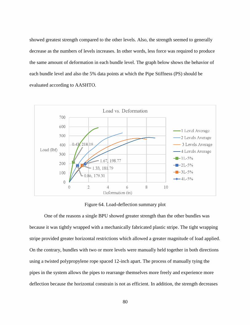
80

showed greatest strength compared to the other levels. Also, the strength seemed to generally

decrease as the numbers of levels increases. In other words, less force was required to produce

the same amount of deformation in each bundle level. The graph below shows the behavior of

each bundle level and also the 5% data points at which the Pipe Stiffness (PS) should be

evaluated according to AASHTO.

Figure 64. Load-deflection summary plot

One of the reasons a single BPU showed greater strength than the other bundles was

because it was tightly wrapped with a mechanically fabricated plastic stripe. The tight wrapping

stripe provided greater horizontal restrictions which allowed a greater magnitude of load applied.

On the contrary, bundles with two or more levels were manually held together in both directions

using a twisted polypropylene rope spaced 12-inch apart. The process of manually tying the

pipes in the system allows the pipes to rearrange themselves more freely and experience more

deflection because the horizontal constrain is not as efficient. In addition, the strength decreases

81

with the increasing number of levels as shown in Figure 64, which is caused to the greater

amount of flexible points in the system.

The next step after establishing the relationship of load-deflection was to calculate the PS

for each bundle. An alternate formula was proposed to calculate the pipe stiffness of multiple

pipes in Chapter 3. The two type of PS were calculated and referred as PS 1 and PS 2.

PS 1 was calculated by following the original formula (24), which neglected the number of

pipes in contact with the loading plate. The method PS 2 is the proposed method to calculate PS

including the number of pipes that were in contact with the loading plate. Once both PS values

were calculated, the percentage of PS reduction from each level was determined. The table below

presents the average value for each level and the PS reduction from each level (See Table 2).

Table 2. Average values for each level and PS reduction

Number

of Levels

5%

Def.

(in)

Force at

5% Def.

(lbf)

PS 1

(lbf/in/in)

PS 2

(lbf/in2/in)

PS

Reduction

(1)

PS

Reduction

(2)

1 0.43 218 60.7 30.4 0% 0%

2 0.86 179 24.9 12.5 59% 59%

3 1.28 159 14.9 7.4 75% 40%

4 1.67 199 12.6 6.3 79% 15%

NOTES: - PS 1 = 1 contact area (original formula)

- PS 2 = 2 contact areas (2 pipes is contact with plate)

PS Reduction (1) is the percent of Pipe Stiffness lost with the respect to the bundle with 1 Level.

PS Reduction (2) is the percent of Pipe Stiffness lost with the respect to the previous level.

82

Table 2 shows the 5% deflection for each bundle with the corresponding number of

levels, the force required to cause that deflection, PS values calculated based on the particular

approach, and two columns showing the strength reduction compared to the first level or the

previous bundle level. Based on the findings, the bundle with only one level showed the greatest

PS value. Also, the greatest PS reduction occurred when the first additional level was added. The

reason for this outcome might be due to the rigidity of a single BPU, which is assembled tightly

wrapped with a mechanically fabricated plastic stripe. Any additional bundle is manually held

together in both directions using a twisted polypropylene rope spaced 12-inch apart, which

makes the system significantly more flexible. The PS reduction itself also decreases with the

addition of bundles.

In addition, a third method of PS was discussed. This method consisted on combining the

total wall area of pipe bundle and establishing new single pipe with equal wall area. The original

formula can now be considered appropriate since the only one line of contact is assumed. Since

the area of multiple pipes was concentrated into one pipe, the new single pipe featured a greater

diameter and wall thickness. Since the new deflection value is used, the average load-deflection

curve for the corresponding level can be used to extrapolate the force needed to cause that

deflection. The following table will provide the results for all three methods:

Table 3. Comparison between PS methods

Number

of

Levels

PS 1

(lb/in2/in)

PS 2

(lb/in/in)

Equivalent

Pipe Area

(lb/in/in)

1 61 31 61

2 25 12 25

3 15 7 25

4 13 6 15

83

From the table above, it can be concluded that PS 1 and the equivalent pipe area method

revealed almost identical PS values. This similarity in values could be because the proportion

between load and deflection remains constant. Even though the idealized pipe with bigger

diameter has a greater value for the 5% deflection, the PS value is normalized because the

corresponding load is also greater because it is extracted from the same curve.

Long BPU’s (37 inches)

BPU’s with 37 inches of length were also tested under the AASHTO M252 is ASTM

D2412 − 11 “Determination of External Loading Characteristics of Plastic Pipe by Parallel-

Plate Loading”. The procedure was similar to the short BPU’s except that three BPU’s are used

in each level and only load values were provided by the testing equipment, not deformation.

Thus, deformation of the pipe bundle was obtained by stopping the loading procedure and

measuring the elevation of the top plate with the use of the laser position sensor. The other

difference was that bigger materials were required for testing. For example, the loading plates

had the same thickness but the length and width were 38 inches. Also, steel toes were welded to

the outside perimeter of the plates to minimize bending of the plates. An image can be seen on

Figure 65.

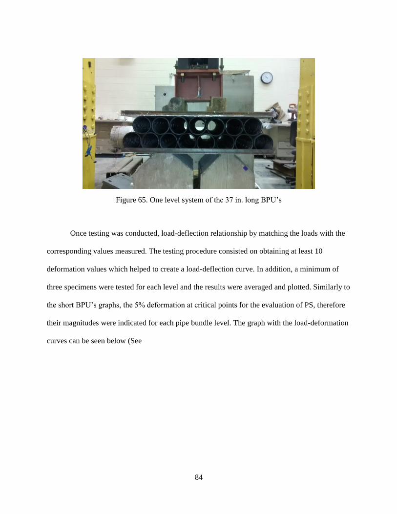
84

Figure 65. One level system of the 37 in. long BPU’s

Once testing was conducted, load-deflection relationship by matching the loads with the

corresponding values measured. The testing procedure consisted on obtaining at least 10

deformation values which helped to create a load-deflection curve. In addition, a minimum of

three specimens were tested for each level and the results were averaged and plotted. Similarly to

the short BPU’s graphs, the 5% deformation at critical points for the evaluation of PS, therefore

their magnitudes were indicated for each pipe bundle level. The graph with the load-deformation

curves can be seen below (See

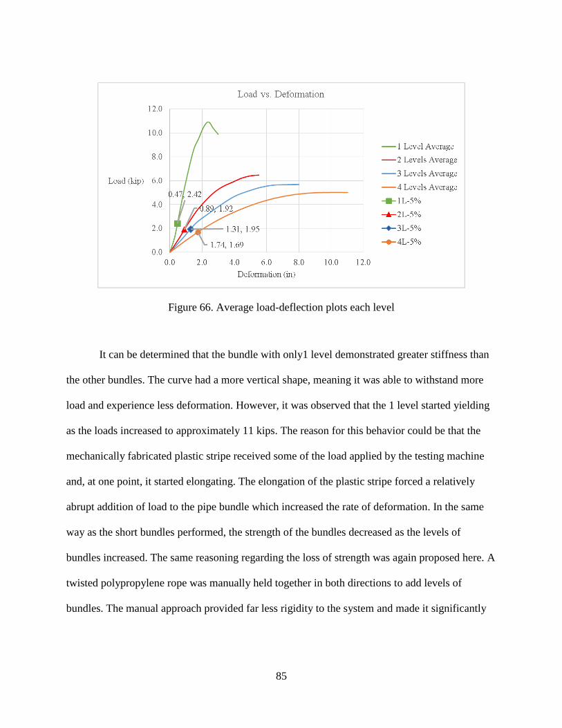
85

Figure 66. Average load-deflection plots each level

It can be determined that the bundle with only1 level demonstrated greater stiffness than

the other bundles. The curve had a more vertical shape, meaning it was able to withstand more

load and experience less deformation. However, it was observed that the 1 level started yielding

as the loads increased to approximately 11 kips. The reason for this behavior could be that the

mechanically fabricated plastic stripe received some of the load applied by the testing machine

and, at one point, it started elongating. The elongation of the plastic stripe forced a relatively

abrupt addition of load to the pipe bundle which increased the rate of deformation. In the same

way as the short bundles performed, the strength of the bundles decreased as the levels of

bundles increased. The same reasoning regarding the loss of strength was again proposed here. A

twisted polypropylene rope was manually held together in both directions to add levels of

bundles. The manual approach provided far less rigidity to the system and made it significantly

86

more susceptible to experience deformation. PS 1 and PS 2 values were calculated just as before

for the long BPU’s and the values can be found below (See Table 4):

Table 4. PS values for 37 inches long BPU’s

Number

of

Levels

5%

Deformation

(in)

Force at

5% Def.

(kip)

PS 1

(lb/in/in)

PS 2

(lb/in2/in)

PS

Reduction

(1)

PS

Reduction

(2)

1 0.466 2.420 206.878 29.554 0% 0%

2 0.893 1.917 85.547 12.221 59% 59%

3 1.306 1.951 59.504 8.501 71% 30%

4 1.737 1.690 38.747 5.535 81% 35%

NOTES: - PS 1 = 1 contact area (original formula)

- PS 2 = 2 contact areas (2 pipes is contact with plate)

PS Reduction (1) is the percent of Pipe Stiffness lost with the respect to the bundle with 1 Level.

PS Reduction (2) is the percent of Pipe Stiffness lost with the respect to the previous level.

It can be observed from Table 4 that again the system 1 demonstrated the highest PS

value compared to the rest of the bundles. The other similarity to the short bundles was that the

greatest drop in PS occurred after the first level of bundle was added. The reason for the

magnitude of that drop was because was regarding the wrapping procedure as mentioned before.

In addition, a greater difference between PS 1 and PS 2 was also observed. The greater

difference in PS values was due to the greater number of pipes in contact with the plate

accounted in the proposed method. The PS value calculated by considering a single pipe with an

equal was also considered and the values can be found in Table 5:

87

Table 5. PS values for the long BPU’s

Number

of

Levels

PS 1 (lb/in2/in) PS 2 (lb/in/in)

Equivalent

Pipe Area

(lb/in/in)

1 206.88 29.55 231.01

2 85.55 12.22 85.59

3 59.50 8.50 46.19

4 38.75 5.54 38.18

Previously, it was found that the equivalent area approach was relatively close to the PS 1

values. Subsequently, the PS 1 and the equivalent pipe area approach were again relatively

similar for all levels of long BPU’s. The reason for the similarity might again be due to the linear

behavior at the strain range evaluated. In other words, the proportion between load-deflection is

constant and evaluating a single pipe with a lightly greater diameter would not cause much of a

difference.

Comparison of short vs long BPU’s

By comparing values for the short BPU’s (Table 4) and the long BPU’s (Table 5), it can

be observed that PS 1 values are higher for the long BPU’s. The reasoning for this outcome

might be that the pressure applied by the loading plate is distributed over a greater area on the

long BPU’s. Since the equation does not consider the number of pipes, PS values would tend to

be higher when the number of pipes used increases. On the other, PS 2 was observed to be

relatively similar between the two bundle lengths. The reason for the similarity could be that the

load applied is normalized by the proposed equation, which does account for the number of pipes

in contact with the loading plate. Therefore, including the number of pipes while evaluating

systems with multiple types might be an effective tool when strength comparison is desired.

88

Field testing

Field testing was considered important to understand the effects of real loads such the

ones exerted by earth pressure and vehicles. Also, the pipe-soil interaction experienced in the

field might have a different effect on the system which could not have been observed in the

laboratory. The setup of the field test included a range of cover depths and configurations and by

keeping the system constant, the difference in the results showed mainly the effects of the cover

characteristics. The truck used for testing had a total gross weight of 66,240 lbf. and each axle

weighed approximately 22 kips. Both of the rear axles did 30 runs each in the forward and

backward direction. Once testing was done on all systems, the data was extracted to Excel for the

determination of the deformation. Plots were observed to have some noise that could had been

produced from other devices connected, environmental effects and so on. Noise in the data could

cause imprecise results which could lead to wrong conclusions and recommendations. One sign

that suggested the presence of noise was the visible deformations recorded observed during times

where the truck did not pass by, for example in the time interval between 600 seconds and 850

seconds of the readings of sensor 2. A plot with raw data of sensor 2 is shown below. (See Figure

67)

89

Figure 67. Plot of sensor 2 showing noise in the data

The noise might have been misleading in sense that they would show a greater drop that

the sensor really experienced. Thus, the noise in the data was also manually eliminated in Excel

for illustration purposes and for a better understanding of deformation readings. An example of

the data corresponding to Sensor 1 can be seen on Figure 68. Plots for the rest of the sensors can

be found in APPENDIX D.

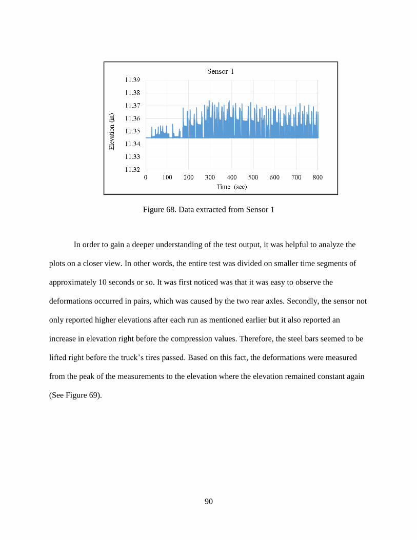
90

Figure 68. Data extracted from Sensor 1

In order to gain a deeper understanding of the test output, it was helpful to analyze the

plots on a closer view. In other words, the entire test was divided on smaller time segments of

approximately 10 seconds or so. It was first noticed was that it was easy to observe the

deformations occurred in pairs, which was caused by the two rear axles. Secondly, the sensor not

only reported higher elevations after each run as mentioned earlier but it also reported an

increase in elevation right before the compression values. Therefore, the steel bars seemed to be

lifted right before the truck’s tires passed. Based on this fact, the deformations were measured

from the peak of the measurements to the elevation where the elevation remained constant again

(See Figure 69).

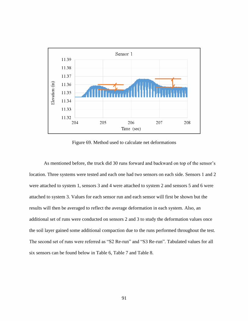
91

Figure 69. Method used to calculate net deformations

As mentioned before, the truck did 30 runs forward and backward on top of the sensor’s

location. Three systems were tested and each one had two sensors on each side. Sensors 1 and 2

were attached to system 1, sensors 3 and 4 were attached to system 2 and sensors 5 and 6 were

attached to system 3. Values for each sensor run and each sensor will first be shown but the

results will then be averaged to reflect the average deformation in each system. Also, an

additional set of runs were conducted on sensors 2 and 3 to study the deformation values once

the soil layer gained some additional compaction due to the runs performed throughout the test.

The second set of runs were referred as “S2 Re-run” and “S3 Re-run”. Tabulated values for all

six sensors can be found below in Table 6, Table 7 and Table 8.

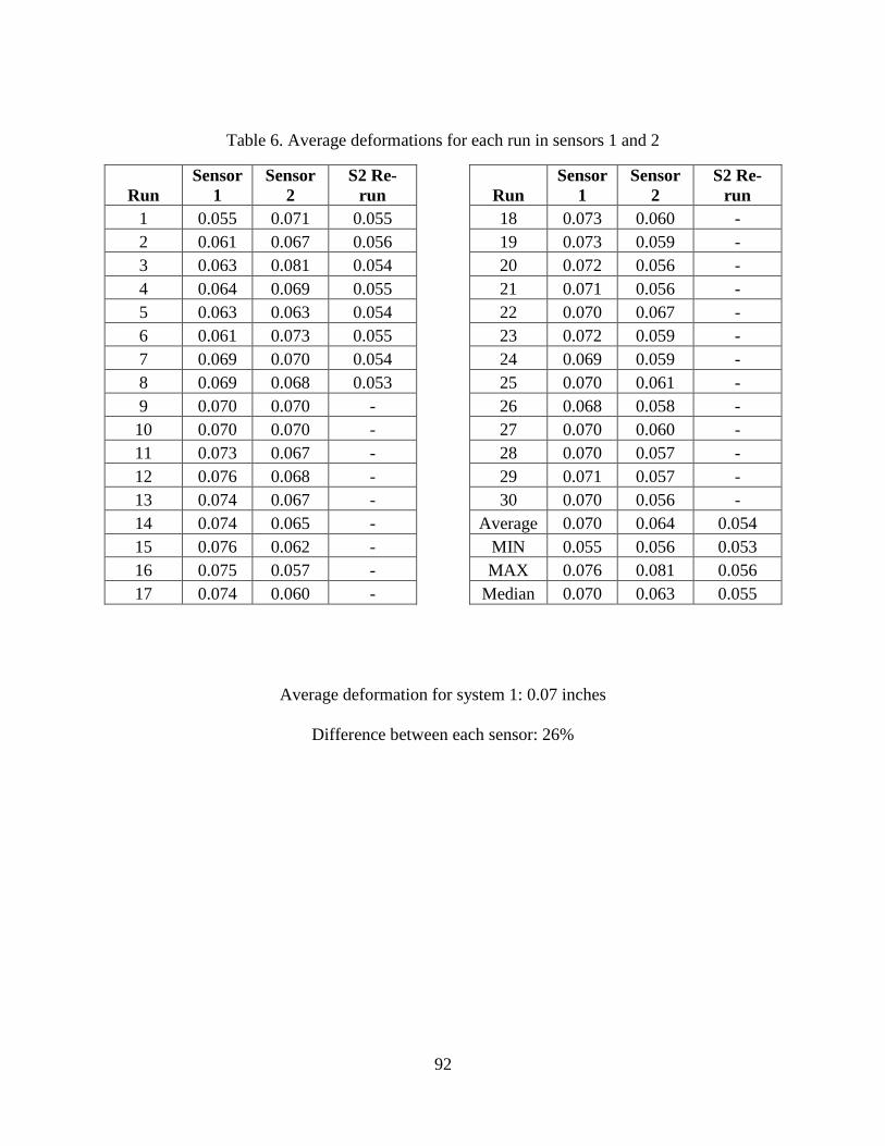
92

Table 6. Average deformations for each run in sensors 1 and 2

Run

Sensor

1

Sensor

2

S2 Re-

run

1 0.055 0.071 0.055

2 0.061 0.067 0.056

3 0.063 0.081 0.054

4 0.064 0.069 0.055

5 0.063 0.063 0.054

6 0.061 0.073 0.055

7 0.069 0.070 0.054

8 0.069 0.068 0.053

9 0.070 0.070 -

10 0.070 0.070 -

11 0.073 0.067 -

12 0.076 0.068 -

13 0.074 0.067 -

14 0.074 0.065 -

15 0.076 0.062 -

16 0.075 0.057 -

17 0.074 0.060 -

Run

Sensor

1

Sensor

2

S2 Re-

run

18 0.073 0.060 -

19 0.073 0.059 -

20 0.072 0.056 -

21 0.071 0.056 -

22 0.070 0.067 -

23 0.072 0.059 -

24 0.069 0.059 -

25 0.070 0.061 -

26 0.068 0.058 -

27 0.070 0.060 -

28 0.070 0.057 -

29 0.071 0.057 -

30 0.070 0.056 -

Average 0.070 0.064 0.054

MIN 0.055 0.056 0.053

MAX 0.076 0.081 0.056

Median 0.070 0.063 0.055

Average deformation for system 1: 0.07 inches

Difference between each sensor: 26%

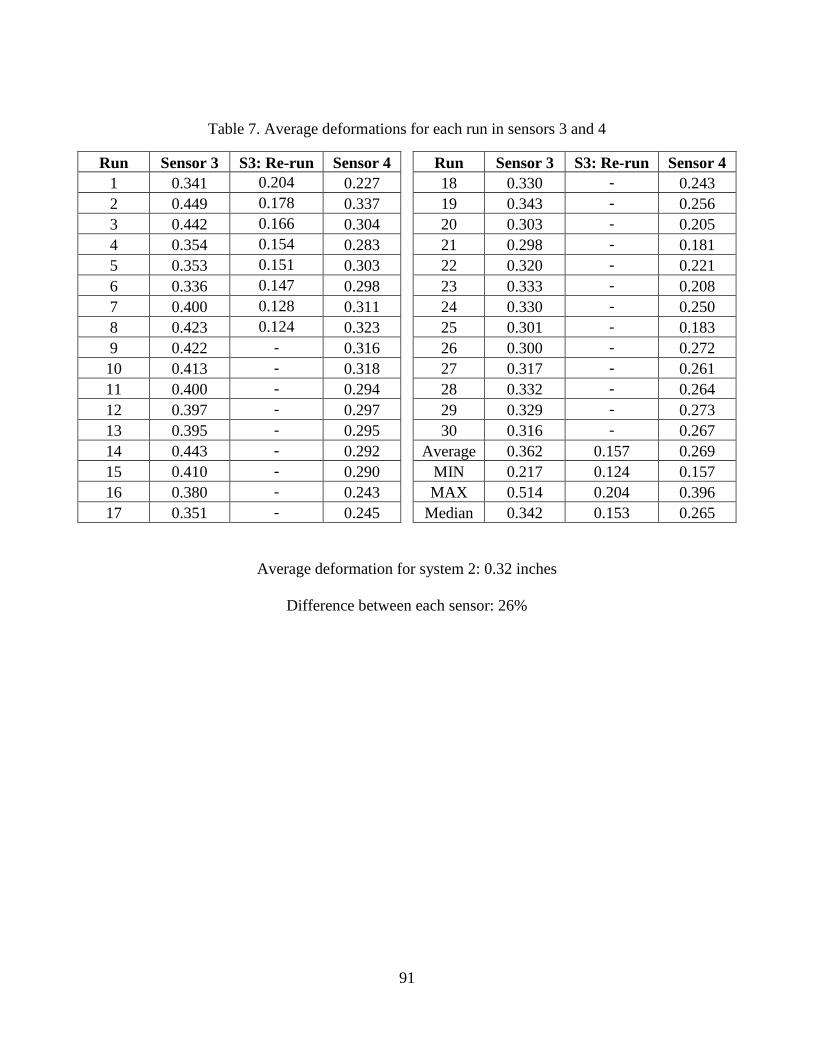
91


Run Sensor 3 S3: Re-run Sensor 4

1 0.341 0.204 0.227

2 0.449 0.178 0.337

3 0.442 0.166 0.304

4 0.354 0.154 0.283

5 0.353 0.151 0.303

6 0.336 0.147 0.298

7 0.400 0.128 0.311

8 0.423 0.124 0.323

9 0.422 - 0.316

10 0.413 - 0.318

11 0.400 - 0.294

12 0.397 - 0.297

13 0.395 - 0.295

14 0.443 - 0.292

15 0.410 - 0.290

16 0.380 - 0.243

17 0.351 - 0.245

Run Sensor 3 S3: Re-run Sensor 4

18 0.330 - 0.243

19 0.343 - 0.256

20 0.303 - 0.205

21 0.298 - 0.181

22 0.320 - 0.221

23 0.333 - 0.208

24 0.330 - 0.250

25 0.301 - 0.183

26 0.300 - 0.272

27 0.317 - 0.261

28 0.332 - 0.264

29 0.329 - 0.273

30 0.316 - 0.267

Average 0.362 0.157 0.269

MIN 0.217 0.124 0.157

MAX 0.514 0.204 0.396

Median 0.342 0.153 0.265



92


Run Sensor 5 Sensor 6

1 1.157 0.806

2 1.256 0.851

3 0.970 0.922

4 0.715 0.944

5 0.925 0.935

6 0.745 0.893

7 0.653 0.880

8 0.714 0.940

9 0.660 0.938

10 0.661 0.982

11 0.620 0.923

12 0.567 0.938

13 0.520 0.965

14 0.505 0.947

15 0.636 0.643

16 0.507 0.571

17 0.493 0.617

18 0.471 0.565

Run Sensor 5 Sensor 6

19 0.415 0.578

20 0.370 0.559

21 0.364 0.548

22 0.325 0.553

23 0.285 0.540

24 0.324 0.538

25 0.310 0.528

26 0.322 0.538

27 0.196 0.528

28 0.175 0.548

29 0.216 0.543

30 0.216 0.569

Average 0.543 0.733

MIN 0.109 0.518

MAX 1.295 1.024

Median 0.492 0.630



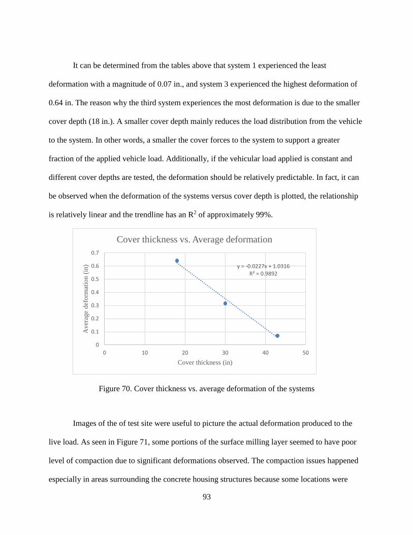
93

It can be determined from the tables above that system 1 experienced the least

deformation with a magnitude of 0.07 in., and system 3 experienced the highest deformation of

0.64 in. The reason why the third system experiences the most deformation is due to the smaller

cover depth (18 in.). A smaller cover depth mainly reduces the load distribution from the vehicle

to the system. In other words, a smaller the cover forces to the system to support a greater

fraction of the applied vehicle load. Additionally, if the vehicular load applied is constant and

different cover depths are tested, the deformation should be relatively predictable. In fact, it can

be observed when the deformation of the systems versus cover depth is plotted, the relationship

is relatively linear and the trendline has an R2 of approximately 99%.

Figure 70. Cover thickness vs. average deformation of the systems

Images of the of test site were useful to picture the actual deformation produced to the

live load. As seen in Figure 71, some portions of the surface milling layer seemed to have poor

level of compaction due to significant deformations observed. The compaction issues happened

especially in areas surrounding the concrete housing structures because some locations were

y = -0.0227x + 1.0316R² = 0.9892

0

0.1

0.2

0.3

0.4

0.5

0.6

0.7

0 10 20 30 40 50

Aver

age

def

orm

atio

n (

in)

Cover thickness (in)

Cover thickness vs. Average deformation

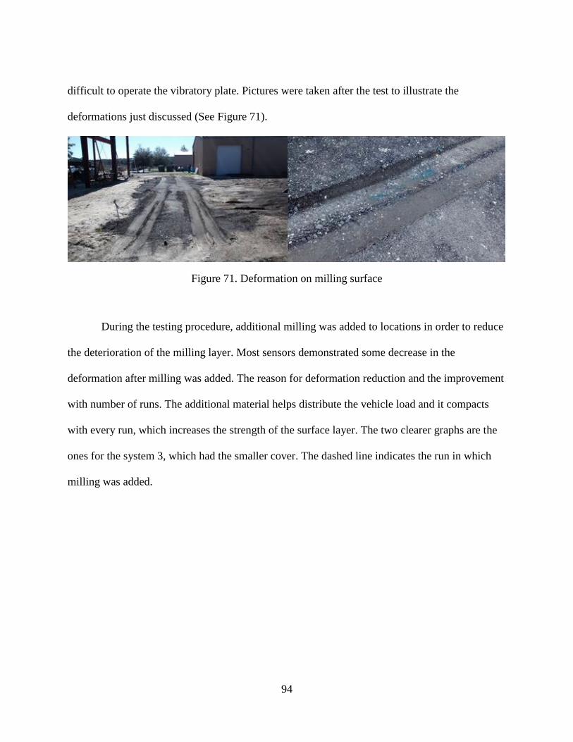
94

difficult to operate the vibratory plate. Pictures were taken after the test to illustrate the

deformations just discussed (See Figure 71).

Figure 71. Deformation on milling surface

During the testing procedure, additional milling was added to locations in order to reduce

the deterioration of the milling layer. Most sensors demonstrated some decrease in the

deformation after milling was added. The reason for deformation reduction and the improvement

with number of runs. The additional material helps distribute the vehicle load and it compacts

with every run, which increases the strength of the surface layer. The two clearer graphs are the

ones for the system 3, which had the smaller cover. The dashed line indicates the run in which

milling was added.

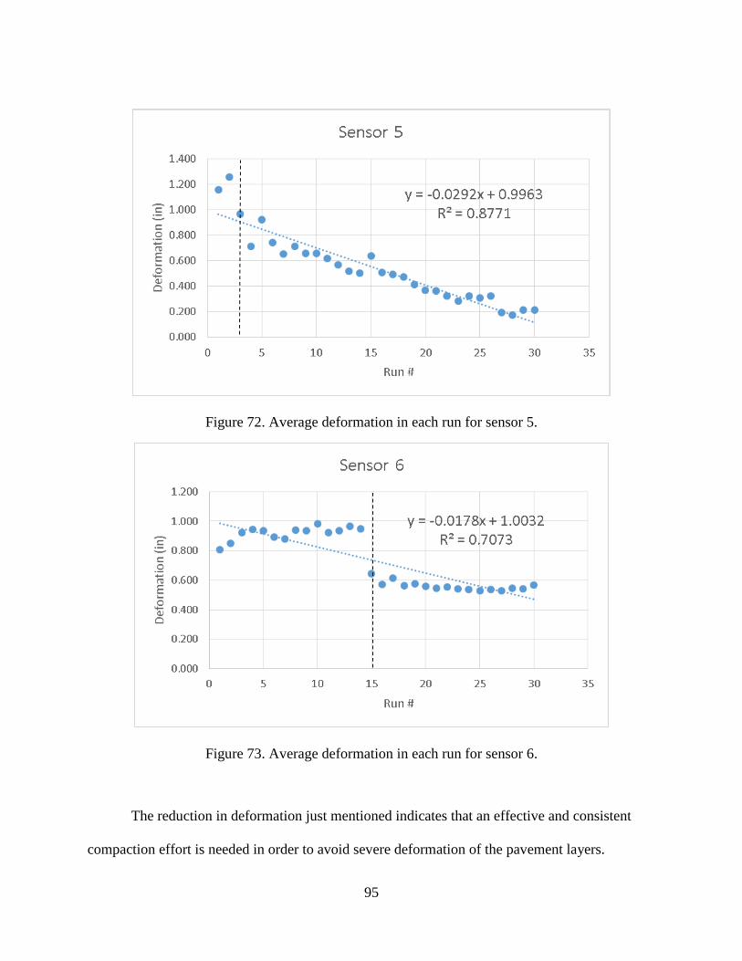
95

Figure 72. Average deformation in each run for sensor 5.

Figure 73. Average deformation in each run for sensor 6.

The reduction in deformation just mentioned indicates that an effective and consistent

compaction effort is needed in order to avoid severe deformation of the pavement layers.

96

Nonetheless, conventional designs of the pipe systems will not have face the problems during the

compaction process because no housing structure is required.

Average values are considered for each cover depth but it was also important to analyze the

variability in dataset. Thus, a boxplot was produced to help visualize the variability of the

deformation for each sensor. A boxplot is a visual statistical approach which displays the

minimum, first quartile, second quartile (or median), third quartile and maximum points in a data

set (See Figure 74).

Figure 74. Boxplot of deformations versus sensors.

The figure above shows a boxplot of the deformations from each sensor. In this case, it

can be determined that sensor 1 and sensor 2 showed no significant difference compared to the

other measurements. Some difference is variability can be observed sensors 3 and 4, but the

variability increases in sensors 5 and 6. The degree of variability might be explained by the

Sensor 6Sensor 5Sensor 4Sensor 3Sensor 2Sensor 1

1.4

1.2

1.0

0.8

0.6

0.4

0.2

0.0

Sensors

Defo

rmati

on

(in

)

Boxplot of deformation for each sensor

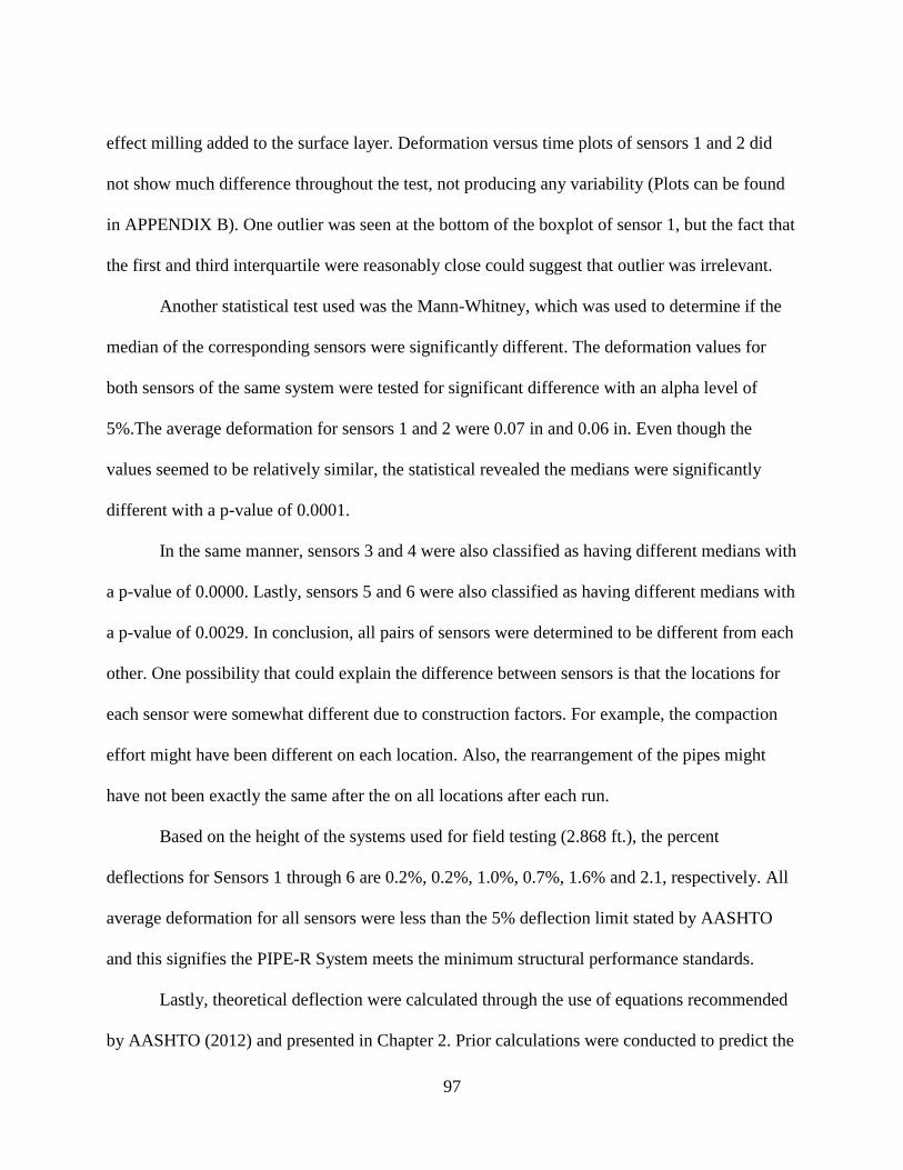
97

effect milling added to the surface layer. Deformation versus time plots of sensors 1 and 2 did

not show much difference throughout the test, not producing any variability (Plots can be found

in APPENDIX B). One outlier was seen at the bottom of the boxplot of sensor 1, but the fact that

the first and third interquartile were reasonably close could suggest that outlier was irrelevant.

Another statistical test used was the Mann-Whitney, which was used to determine if the

median of the corresponding sensors were significantly different. The deformation values for

both sensors of the same system were tested for significant difference with an alpha level of

5%.The average deformation for sensors 1 and 2 were 0.07 in and 0.06 in. Even though the

values seemed to be relatively similar, the statistical revealed the medians were significantly

different with a p-value of 0.0001.

In the same manner, sensors 3 and 4 were also classified as having different medians with

a p-value of 0.0000. Lastly, sensors 5 and 6 were also classified as having different medians with

a p-value of 0.0029. In conclusion, all pairs of sensors were determined to be different from each

other. One possibility that could explain the difference between sensors is that the locations for

each sensor were somewhat different due to construction factors. For example, the compaction

effort might have been different on each location. Also, the rearrangement of the pipes might

have not been exactly the same after the on all locations after each run.

Based on the height of the systems used for field testing (2.868 ft.), the percent

deflections for Sensors 1 through 6 are 0.2%, 0.2%, 1.0%, 0.7%, 1.6% and 2.1, respectively. All

average deformation for all sensors were less than the 5% deflection limit stated by AASHTO

and this signifies the PIPE-R System meets the minimum structural performance standards.

Lastly, theoretical deflection were calculated through the use of equations recommended

by AASHTO (2012) and presented in Chapter 2. Prior calculations were conducted to predict the

98

magnitude of dead loads and live loads acting on the system. Afterwards, the thrust on the pipe

was utilized to calculate the theoretical deflection values. The estimated deflection was

approximately 0.23 inches for all three systems. The reason a similar deflection was predicted for

different cover properties was because the modulus of elasticity was a significant high value

which reduced the impact of slight differences in the load. An important factor to consider was

that the equations were designed for single pipes, and not a system of pipes such as the one

evaluated in this study. Therefore, there is no direct comparison of this result and the

deformations found in the field testing.

99

CHAPTER 5: CONCLUSION

Water scarcity continues to be a problem that affects a significant fraction of the world’s

population. Water harvesting is one approach that could help alleviate some of the effects of

water related issues. This study evaluated the ability of the Microsoft Excel based model called

PIPE-R Model to predict water harvesting operations of an underground pipe systems based on

available hourly precipitation data. The PIPE-R Model will also help the user adjust properties

and dimensions of the system in order to achieve a particular efficiency desired. From the results

of the study in can be observed that the PIPE-R Model is an effective tool to forecast the average

yearly values of a proposed system such hydrologic efficiency, water supplied and groundwater

recharge.

The structural integrity of the pipes used for the water harvesting system was also

evaluated. Laboratory and field testing were conducted on the pipes to study their behavior under

load effects. Results from the laboratory revealed that single pipes met the minimum

specifications specified by AASHTO M252 and that the pipes rebound ratio of about 96%. The

pipes were also bundled in groups of five and tested for strength purposes. The results of these

loading tests determined that a single bundle unit pipe (BPU) performs better than multilevel

systems due to increasing flexibility in the system. Also, long BPU showed greater strength than

short BPU based on the PS 1 equation and the reason is that the load was distributed over a

greater number of pipes while the equation does not account for the number of pipes in contact.

However, by considering the number of pipes in contact using the proposed formula PS 2, the PS

values seemed to be relatively similar for both lengths. Subsequently, the proposed equation is an

effective tool to analyze systems that use multiple pipes. Lastly, a third method to calculate PS

100

was proposed and the purpose was to translate systems of pipes to a single pipe with equivalent

wall area which would allow the original PS equation to be more applicable. Once the single

pipes were established and evaluated, the results were observed to be similar to PS 2 equation.

Field testing revealed that the height of cover has an effect on the deformation

experienced by the pipes at each sensor location under dead and live load effects. The average

deformations found for the cover depths of 43 in, 30 in and 18 in were 0.07 in, 0.32 in and 0.64

in, respectively. The deformations found were all under the 5% deflection limit stated by

AASHTO. Based on these results, it is recommended that a minimum of 30 inches of cover be

provided if live loads are present.

101

APPENDIX A: SYSTEM AVERAGE DEFORMATION VERSUS NUMBER

OF RUNS

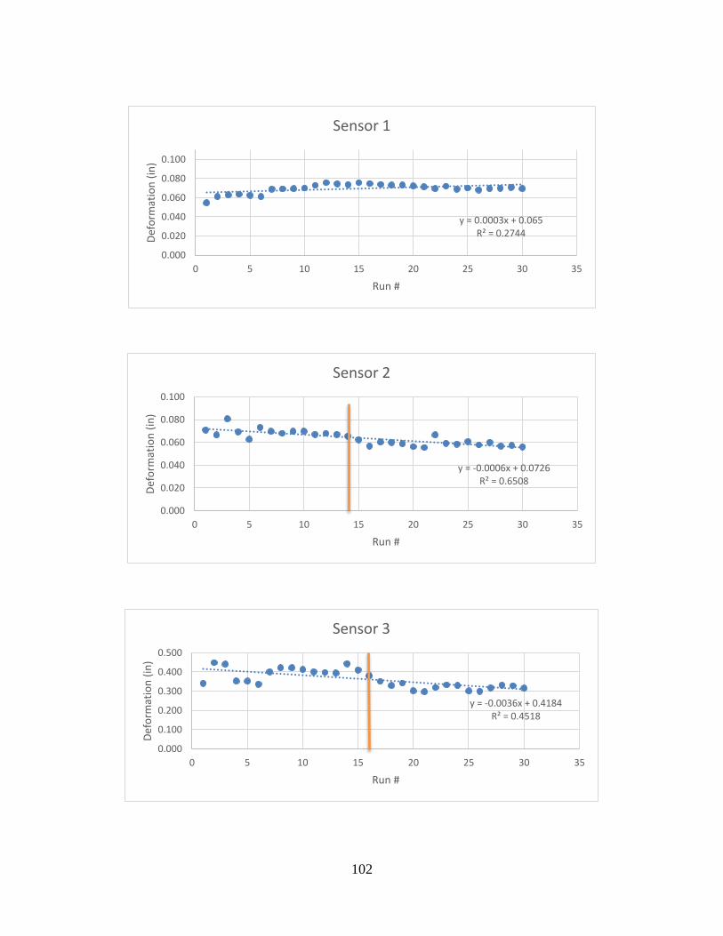
102

y = 0.0003x + 0.065R² = 0.2744

0.000

0.020

0.040

0.060

0.080

0.100

0 5 10 15 20 25 30 35

Def

orm

atio

n (

in)

Run #

Sensor 1

y = -0.0006x + 0.0726R² = 0.6508

0.000

0.020

0.040

0.060

0.080

0.100

0 5 10 15 20 25 30 35

Def

orm

atio

n (

in)

Run #

Sensor 2

y = -0.0036x + 0.4184R² = 0.4518

0.000

0.100

0.200

0.300

0.400

0.500

0 5 10 15 20 25 30 35

Def

orm

atio

n (

in)

Run #

Sensor 3

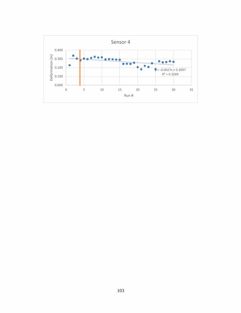
103

y = -0.0027x + 0.3097R² = 0.3169

0.000

0.100

0.200

0.300

0.400

0 5 10 15 20 25 30 35

Def

orm

atio

n (

in)

Run #

Sensor 4

104

APPENDIX B: SENSOR MEASUREMENTS

108

REFERENCES

AASHTO (2003). M252: Standard Specification for Corrugated Polyethylene Drainage Pipe.

Washington, D.C.

AASHTO (2012). LRFD Bridge Design Specifications. Washington, DC.

Arockiasamy, M., et al. (2006). "Full-scale field tests on flexible pipes under live load

application." Journal of performance of constructed facilities 20(1): 21-27.

Asgarzadeh, H., et al. (2014). "Determination of soil available water for plants: Consistency

between laboratory and field measurements." Geoderma 226: 8-20.

Barker, R. M. and J. A. Puckett (2013). Design of highway bridges: An LRFD approach, John

wiley & sons.

Bilgin, Ö. (2013). "Modeling Viscoelastic Behavior of Polyethylene Pipe Stresses." Journal of

Materials in Civil Engineering 26(4): 676-683.

Brookes, J. D. and C. C. Carey (2011). "Resilience to blooms." Science 334(6052): 46-47.

Burns, J. Q. and R. M. Richard (1964). Attenuation of stresses for buried cylinders. Proceedings

of the Symposium on Soil-Structure Intenaction, September 1974.

Cesaraccio, C., et al. (2001). "An improved model for determining degree-day values from daily

temperature data." International Journal of Biometeorology 45(4): 161-169.

Chaudhuri, S. and S. Ale (2014). "Long term (1960–2010) trends in groundwater contamination

and salinization in the Ogallala aquifer in Texas." Journal of Hydrology 513: 376-390.

Chu, S. T. (1978). "Infiltration during an unsteady rain." Water Resources Research 14(3): 461-

466.

Dixon, A., et al. (1999). "Water saving potential of domestic water reuse systems using

greywater and rainwater in combination." Water Science and Technology 39(5): 25-32.

EPA (2011). Water Quality Standards Handbook: Chapter 3. Washington, D.C. .

EPA (2013). "Water Recycling and Reuse: The Environmental Benefits." Retrieved 10/09/2014,

from http://www.epa.gov/region9/water/recycling/.

Faragher, E., et al. (2000). "Analysis of repeated-load field testing of buried plastic pipes."

Journal of transportation engineering 126(3): 271-277.

http://www.epa.gov/region9/water/recycling/

109

Folkman, S. L. and A. Moser (2002). "The Structural Performance of a Storm Water Detention

System Utilizing Bundled HDPE Pipes."

Gebregiorgis, M. F. and M. J. Savage (2007). "Field, laboratory and estimated soil-water content

limits." Water SA 32(2): 155-162.

Gleeson, T., et al. (2010). "Groundwater sustainability strategies." Nature Geoscience 3(6): 378-

379.

Green, W. H. and G. Ampt (1911). "Studies on Soil Phyics." The Journal of Agricultural Science

4(01): 1-24.

Gutentag, E. D. (1984). "Geohydrology of the High Plains aquifer in parts of Colorado, Kansas,

Nebraska, New Mexico, Oklahoma, South Dakota, Texas, and Wyoming: High Plains RASA

Project [Western States (USA); South Central States (USA)]." Geological Survey professional

paper (USA).

Harbor, J. (1999). "Engineering geomorphology at the cutting edge of land disturbance: erosion

and sediment control on construction sites." Geomorphology 31: 247-263.

Hardin, M. (2006). The effectiveness of a specifically designed green roof stormwater treatment

system irrigated with recycled stormwater runoff to achieve pollutant removal and stormwater

volume reduction, University of Central Florida Orlando, Florida.

Hardin, M. (2006). The effectiveness of a specifically designed green roof stormwater treatment

system irrigated with recycled stormwater runoff to achieve pollutant removal and stormwater

volume reduction: Green Roof System Boundaries.

Hardin, M., et al. (2012). "A Mass Balance Model for Designing Green Roof Systems that

Incorporate a Cistern for Re-Use." Water 4(4): 914-931.

Harper, H. H. and D. M. Baker (2007). Evaluation of current stormwater design criteria within

the state of Florida, Orlando, Florida: Environmental Research & Design, Inc.

Helalia, A. M. (1993). "The relation between soil infiltration and effective porosity in different

soils." Agricultural water management 24(1): 39-47.

Hoeg, K. (1966). Pressure distribution on underground structural cylinders, DTIC Document.

Holtan, H. N. (1961). "Concept for infiltration estimates in watershed engineering."

J. Doorenbos and W. O. Pruitt (1984). " Guidelines for predicting crop water requirements."

FAO Irrigation and Drainage Paper 24.

110

Jeyapalan, J. K. and B. Boldon (1986). "Performance and selection of rigid and flexible pipes."


Juday, D. G., et al. (2011). "Use of alternative temperature expressions with Blaney-Criddle."

Journal of Irrigation and Drainage Engineering 137(9): 573-584.

Kang, J. S., et al. (2009). "Short-term and long-term behaviors of buried corrugated high-density

polyethylene (HDPE) pipes." Composites Part B: Engineering 40(5): 404-412.

Khatri, D. K., et al. (2013). "Laboratory evaluation of deformations of steel-reinforced high-

density polyethylene pipes under static loads." Journal of Materials in Civil Engineering 25(12):

1964-1969.

Kissin, Y. V. (2012). Polyethylene: end-use properties and their physical meaning, Carl Hanser

Verlag GmbH Co KG.

Krishnaswamy, R. K. (2005). "Analysis of ductile and brittle failures from creep rupture testing

of high-density polyethylene (HDPE) pipes." Polymer 46(25): 11664-11672.

Langeveld, J. G., et al. (2012). "Uncertainties of stormwater characteristics and removal rates of

stormwater treatment facilities: Implications for stormwater handling." Water Research 46:

6868-6880.

Lay, G. and R. Brachman (2013). "Full-scale physical testing of a buried reinforced concrete

pipe under axle load." Canadian geotechnical journal 51(4): 394-408.

Lee, T., et al. (2001). "Ultrasonic irradiation for blue-green algae bloom control." Environmental

technology 22(4): 383-390.

Leuven, R., et al. (1986). "Effects of water acidification on the distribution pattern and the

reproductive success of amphibians." Experientia 42(5): 495-503.

Liu, G., et al. (2010). "Applicability of the Green-Ampt infiltration model with shallow boundary

conditions." Journal of Hydrologic Engineering 16(3): 266-273.

Maidment, D. R. (1992). Handbook of hydrology, McGraw-Hill Inc.

Marston, A. and A. Anderson (1913). The Theory of Loads on Pipes in Ditches: And Tests of

Cement and Clay Drain Tile and Sewer Pipe, Iowa State College of Agriculture and Mechanic

Arts.

Masada, T. (2000). "Modified Iowa formula for vertical deflection of buried flexible pipe."


111

McIntyre, D. and J. Sleeman (1982). "Macropores and hydraulic conductivity in a swelling soil."

Soil Research 20(3): 251-254.

Mein, R. G. and C. L. Larson (1971). Modeling the infiltration component of the rainfall-runoff

process, Water Resources Research Center, University of Minnesota.

Metcalf, L., et al. (1972). Wastewater engineering: treatment, disposal, and reuse, McGraw-Hill.

Minnesota Pollution Control Agency (2008). Nutrients: Phosphorus, Nitrogen Sources, Impact

on Water Quality St. Paul, MN.

Morel‐Seytoux, H. and J. Khanji (1974). "Derivation of an Equation of Infiltration." Water

Resources Research 10(4): 795-800.

Morteza, N. (2010). Consumptive Use Program Plus (CUP+). 29th Conference on Agricultural

and Forest Meteorology.

Motahari, A. and A. Abolmaali (2009). "Structural deformation characteristics of installed HDPE

circular pipelines." Journal of transportation engineering 136(4): 298-303.

NCHRP (2010). REPORT 647. WASHINGTON, D.C., TRANSPORTATION RESEARCH

BOARD OF THE NATIONAL ACADEMIES. REPORT 647.

O'Connor, C. (2011). "The nature of polyethylene pipe failure." Modern Plastics Worldwide

88(2): 20-22.

Paaijmans, K. P., et al. (2008). "The effect of water turbidity on the near-surface water

temperature of larval habitats of the malaria mosquito Anopheles gambiae." Int J Biometeorol

52: 747–753.

Philip, J. R. (1957). "The theory of infiltration: 4. Sorptivity and algebraic infiltration equations."

Soil science 84(3): 257-264.

Pinckney, J. L., et al. (2001). "The role of nutrient loading and eutrophication in estuarine

ecology." Environmental Health Perspectives 109(Suppl 5): 699.

Rijsberman, F. R. (2006). "Water scarcity: fact or fiction?" Agricultural water management

80(1): 5-22.

Sargand, S. M. and T. Masada (2000). "Performance of large-diameter honeycomb-design HDPE

pipe under a highway embankment." Canadian geotechnical journal 37(5): 1099-1108.

Saxton, K. and W. Rawls (2006). "Soil water characteristic estimates by texture and organic

matter for hydrologic solutions." Soil Science Society of America Journal 70(5): 1569-1578.

112

SCS, U. (1970). "Irrigation Water Requirements." Tech Release(21): 92.

Serrano, S. E. (2001). "Explicit solution to Green and Ampt infiltration equation." Journal of

Hydrologic Engineering 6(4): 336-340.

Shijian, W., et al. (2002). "BIAXIALLY SELF-REINFORCED TRANSPARENT HDPE PIPES

EXTRUDED FROM UNIAXIAL ELONGATIONAL FLOW FIELD [J]." Engineering Plastics

Application 8: 013.

Spangler, M. G. and G. Shafer (1938). The structural design of flexible pipe culverts. Highway

Research Board Proceedings.

Wada, Y., et al. (2010). "Global depletion of groundwater resources." Geophysical Research

Letters 37(20).

Wanielista, M., et al. (2014). "User’s Manual for the BMPTRAINS Model."

Wanielista, M., et al. (1991). "Design curves for the reuse of stormwater." Florida Department of

Environmental Regulation.

Watkins, K. (2006). "Human Development Report 2006-Beyond scarcity: Power, poverty and

the global water crisis." UNDP Human Development Reports (2006).

Watkins, R. K. and M. Spangler (1958). Some characteristics of the modulus of passive

resistance of soil: A study in similitude. Highway Research Board Proceedings.

Zarghami, M. and S. Akbariyeh (2012). "System dynamics modeling for complex urban water

systems: application to the city of Tabriz, Iran." Resources, Conservation and Recycling 60: 99-

106.

Evaluation of Strength and Hydraulic Properties of Buried ...

Documents

Transcript of Evaluation of Strength and Hydraulic Properties of Buried ...