Research, Development, and TechnologyTurner-Fairbank Highway Research Center6300 Georgetown PikeMcLean, VA 22101-2296

July 2006

SHARED-USE PATHSFINAL REPORT

Evaluation of Safety, Design, and Operation of

FOREWORD

Shared paths are paved, off-road facilities designed for travel by a variety of nonmotorized users, including bicyclists, pedestrians, skaters, joggers, and others. Shared-path planners and designers face a serious challenge in determining how wide paths should be and whether the various modes of travel should be separated from each other. Currently, there is very little substantive guidance available to aid in those decisions. This document describes the development of a new method to analyze the quality of service provided by shared paths of various widths and the accommodation of various travel-mode splits. The researchers assembled the new method using new theoretical traffic-flow concepts, a large set of operational data from 15 paths in 10 cities across the United States, and the perceptions of more than 100 path users. Given a count or estimate of the overall path user volume in the design-hour, the new method described here can provide the level of service for path widths from 2.44 to 6.1 meters (8 to 20 feet). The information in this document should be of interest to planners, engineers, parks and recreation professionals, and to others involved in the planning, design, operation, and/or maintenance of shared paths. In addition, this document will be of interest to researchers investigating how to analyze multiple modes of travelers in a finite space with minimal traffic control. This document describes a spreadsheet calculation tool called SUPLOS that was also developed as part of the same effort, and this tool is being circulated by the Federal Highway Administration (FHWA).

Michael F. Trentacoste Director, Office of Safety Research and Development

NOTICE

This document is disseminated under the sponsorship of the U.S. Department of Transportation in the interest of information exchange. The U.S. Government assumes no liability for the use of the information contained in this document. This report does not constitute a standard, specification, or regulation. The U.S. Government does not endorse products or manufacturers. Trademarks or manufacturers’ names appear in this report only because they are considered essential to the objective of the document.

QUALITY ASSURANCE STATEMENT FHWA provides high-quality information to serve Government, industry, and the public in a manner that promotes public understanding. Standards and policies are used to ensure and maximize the quality, objectivity, utility, and integrity of its information. FHWA periodically reviews quality issues and adjusts its programs and processes to ensure continuous quality improvement.

Technical Report Documentation Page 1. Report No. FHWA-HRT-05-137

2. Government Accession No.

3. Recipient’s Catalog No.

5. Report Date July 2006

4. Title and Subtitle Evaluation of Safety, Design, and Operation of Shared-Use Paths—Final Report

6. Performing Organization Code

7. Author(s) J.E. Hummer, N.M. Rouphail, J.L. Toole, R.S. Patten, R.J. Schneider, J.S. Green, R.G. Hughes, and S.J. Fain

8. Performing Organization Report No.

10. Work Unit No. (TRAIS)

9. Performing Organization Name and Address Department of Civil, Construction, and Environmental Engineering North Carolina State University Raleigh, NC 27695

11. Contract or Grant No. DTFH61-00-R-00070

13. Type of Report and Period Covered Final Report September 2000 – May 2005

12. Sponsoring Agency Name and Address Office of Safety Research and Development Federal Highway Administration 6300 Georgetown Pike McLean, VA 22101

14. Sponsoring Agency Code

15. Supplementary Notes: Contracting Officer’s Technical Representative (COTR): Ann Do, HRDS-06 16. Abstract Shared-use paths are becoming increasingly busy in many places in the United States. Path designers and operators need guidance on how wide to make new or rebuilt paths, and on whether to separate the different types of users. The current guidance is not very specific; it has not been calibrated to conditions in the United States, and does not accommodate the range of modes found on a typical U.S. path. The purpose of this project was to develop a level of service (LOS) estimation method for shared-use paths that overcomes these limitations. The research included the development of the theory of traffic flow on a path, an extensive effort to collect data on path operations, and a survey through which path users expressed their degree of satisfaction with the paths shown in a series of videos. Based on the theory developed and the data collected, the researchers developed an LOS estimation method for bicyclists that requires minimal input and produces a simple and useful result. Factors involved in the estimation of an LOS for a path include the number of times a typical bicyclist meets or passes another path user, the number of those passings that are delayed, the path width, and whether the path has a centerline. The method considers four other types of path users besides the adult bicyclists for whom the LOS is calculated—pedestrians, joggers, child bicyclists, and skaters. This report documents the research conducted during the project. Other products of the effort include Report No. FHWA-HRT-05-138, Shared-Use Path Level of Service Calculator: A User’s Guide (for the LOS procedure and the spreadsheet calculation tool); and a TechBrief, Publication No. FHWA-HRT-05-139, Evaluation of Safety, Design, and Operation of Shared-Use Paths. 17. Key Words Path, trail, bicycle, shared use, level of service, width, pedestrian, skater.

18. Distribution Statement No restrictions. This document is available to the public through the National Technical Information Service, Springfield, VA 22161.

19. Security Classif. (of this report) Unclassified

20. Security Classif. (of this page) Unclassified

21. No. of Pages 161

22. Price

Form DOT F 1700.7 (8-72) Reproduction of completed page authorized

ii

SI* (MODERN METRIC) CONVERSION FACTORS APPROXIMATE CONVERSIONS TO SI UNITS

Symbol When You Know Multiply By To Find Symbol LENGTH

in inches 25.4 millimeters mm ft feet 0.305 meters m yd yards 0.914 meters m mi miles 1.61 kilometers km

AREA in2 square inches 645.2 square millimeters mm2

ft2 square feet 0.093 square meters m2

yd2 square yard 0.836 square meters m2

ac acres 0.405 hectares hami2 square miles 2.59 square kilometers km2

VOLUME fl oz fluid ounces 29.57 milliliters mL gal gallons 3.785 liters L ft3 cubic feet 0.028 cubic meters m3

yd3 cubic yards 0.765 cubic meters m3

NOTE: volumes greater than 1000 L shall be shown in m3

MASS oz ounces 28.35 grams glb pounds 0.454 kilograms kgT short tons (2000 lb) 0.907 megagrams (or "metric ton") Mg (or "t")

TEMPERATURE (exact degrees) oF Fahrenheit 5 (F-32)/9 Celsius oC

or (F-32)/1.8 ILLUMINATION

fc foot-candles 10.76 lux lxfl foot-Lamberts 3.426 candela/m2 cd/m2

FORCE and PRESSURE or STRESS lbf poundforce 4.45 newtons N lbf/in2 poundforce per square inch 6.89 kilopascals kPa

APPROXIMATE CONVERSIONS FROM SI UNITS Symbol When You Know Multiply By To Find Symbol

LENGTHmm millimeters 0.039 inches in m meters 3.28 feet ft m meters 1.09 yards yd km kilometers 0.621 miles mi

AREA mm2 square millimeters 0.0016 square inches in2

m2 square meters 10.764 square feet ft2

m2 square meters 1.195 square yards yd2

ha hectares 2.47 acres ackm2 square kilometers 0.386 square miles mi2

VOLUME mL milliliters 0.034 fluid ounces fl oz L liters 0.264 gallons gal m3 cubic meters 35.314 cubic feet ft3

m3 cubic meters 1.307 cubic yards yd3

MASS g grams 0.035 ounces ozkg kilograms 2.202 pounds lbMg (or "t") megagrams (or "metric ton") 1.103 short tons (2000 lb) T

TEMPERATURE (exact degrees) oC Celsius 1.8C+32 Fahrenheit oF

ILLUMINATION lx lux 0.0929 foot-candles fc cd/m2 candela/m2 0.2919 foot-Lamberts fl

FORCE and PRESSURE or STRESS N newtons 0.225 poundforce lbf kPa kilopascals 0.145 poundforce per square inch lbf/in2

*SI is the symbol for th International System of Units. Appropriate rounding should be made to comply with Section 4 of ASTM E380. e(Revised March 2003)

iii

TABLE OF CONTENTS

1. Introduction..................................................................................................................................1

Shared-Use Paths .........................................................................................................................1 Definition .................................................................................................................................1 Gaining Popularity ...................................................................................................................1

Problems Facing Designers..........................................................................................................1 Existing Level of Service (LOS) Method ................................................................................2 Limitations of Current LOS Method........................................................................................2

Project Objective..........................................................................................................................4 Project Methods ...........................................................................................................................4

Development of Theory ...........................................................................................................5 Operational Data Collection ....................................................................................................5 Perceptual Data Collection ......................................................................................................6 A Usable Procedure .................................................................................................................6

Project Scope Limited..................................................................................................................7 Research Products........................................................................................................................8

Description of the Products......................................................................................................8 Intended Users .........................................................................................................................8

Report Format ............................................................................................................................10

2. Literature Review.......................................................................................................................11

Introduction................................................................................................................................11 Path User Characteristics ...........................................................................................................11

Pedestrian Characteristics ......................................................................................................11 Bicyclist Characteristics.........................................................................................................13 Other Path Users ....................................................................................................................16

Measuring Path User Quality of Service ...................................................................................17 Hindrance...............................................................................................................................17 Density ...................................................................................................................................20 Space ......................................................................................................................................21 Stress ......................................................................................................................................21 Current LOS Scales................................................................................................................23 Other Ways To Set the LOS Scale.........................................................................................25

Summary ....................................................................................................................................26

3. Development of Theory .............................................................................................................29

Introduction................................................................................................................................29 Estimating the Number of Events ..............................................................................................29

Glossary of Variables.............................................................................................................30 Estimating Active Passing Events .............................................................................................30

Extension to Exclude Marginal Active Passing Events.........................................................32 Estimating the Number of Passive Passing Events................................................................34 Extension to Exclude Marginal Passive Passing Events........................................................37

iv

Estimating the Number of Meetings ..........................................................................................37 Sensitivity of Passing Events to Key Parameters ..................................................................41

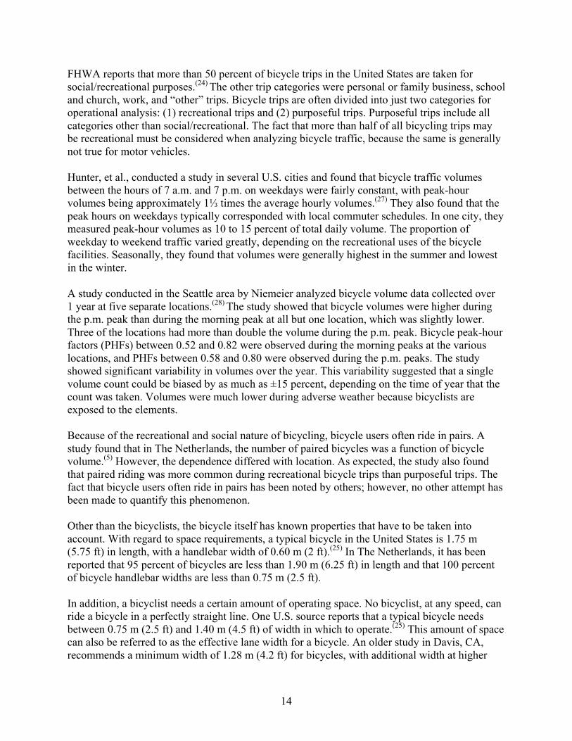
Estimating the Probability of Delayed Passing..........................................................................43 Delayed Passing on Three-Lane Paths...................................................................................46 Delayed Passing on Four-Lane Paths ....................................................................................48 Multimodal Delayed Passing Probability ..............................................................................49 Numerical Application of the Delayed Passing Models ........................................................49

4. Operational Data Collection ......................................................................................................53

Introduction................................................................................................................................53 Data Collection Method.............................................................................................................53

Equipment ..............................................................................................................................54 Site Selection .............................................................................................................................55 Data Collection Execution .........................................................................................................60

5. Operational Data Analysis .........................................................................................................63

Introduction................................................................................................................................63 Average and Default Values ......................................................................................................63

Speed......................................................................................................................................63 Volume and Mode Split .........................................................................................................64 Peak-Hour Factor ...................................................................................................................66 Users Occupying Two Lanes .................................................................................................68 Distance Needed to Pass ........................................................................................................69

Validating Theory ......................................................................................................................71 Speeds Normally Distributed.................................................................................................72 Comparing Predicted Meetings and Passings to Field Data ..................................................77

6. Perception Data Collection ........................................................................................................87

General Rationale.......................................................................................................................87 Participants.................................................................................................................................87 Collection of User Perception Data ...........................................................................................89

Structure and Content of the Survey Instrument....................................................................89 Format of Participants’ Responses.........................................................................................91

7. Analysis of Perception Survey Responses.................................................................................93

Introduction................................................................................................................................93 Data Overview ...........................................................................................................................93

Demographic Variables .........................................................................................................96 Path Design Variables............................................................................................................99 Events on the Path................................................................................................................100 Video Quality.......................................................................................................................103

Model Creation ........................................................................................................................104 Interactions...........................................................................................................................104 Choice of Overall Response.................................................................................................105 Fitting the Model..................................................................................................................106

v

8. LOS Procedure.........................................................................................................................109

Introduction..............................................................................................................................109 Types of Shared-Use Paths To Which This Study Applies .....................................................110 LOS Defined ............................................................................................................................110 The Perception Survey Response Scale...................................................................................111 Developing the LOS Procedure ...............................................................................................113

Start With the Model from Chapter 7 ..................................................................................114 Model Does Not Cover All Combinations...........................................................................114

Delayed Passing Adjustment ...................................................................................................115 Adjustment for Low Number of Events...............................................................................117 Putting It All Together .........................................................................................................117 Comparison to HCM Method ..............................................................................................119

Applying the Model .................................................................................................................121 Link Analysis .......................................................................................................................121 Data Requirements...............................................................................................................123 Assumptions and Default Values.........................................................................................126

LOS Lookup Tables.................................................................................................................127 Instructions for Using the LOS Calculator ..........................................................................127 Implications for Trail Design...............................................................................................129 Trail Width...........................................................................................................................129 Centerline Striping ...............................................................................................................130 Multiple Treadways .............................................................................................................130 Trail Operations and Management.......................................................................................130

Case Studies .............................................................................................................................131

9. Conclusions and Recommendations ........................................................................................133

Introduction..............................................................................................................................133 Conclusions..............................................................................................................................134 Recommendations....................................................................................................................135

Marketing the New LOS Procedure.....................................................................................136 Future Research Needs ........................................................................................................136

Appendix A. Perception Survey Fact Sheet and Informed Consent Form ..................................139

Appendix B. Perception Survey Background Information Form ................................................141

Appendix C. Screen Shots From Perception Study Video ..........................................................143

References....................................................................................................................................149

vi

LIST OF FIGURES Figure 1. Schematic for active passing estimation........................................................................ 31 Figure 2. Schematic for passive passing estimation. .................................................................... 34 Figure 3. Schematic for meeting event estimation........................................................................ 37 Figure 4. Sensitivity of hourly passing rates to individual bicyclist speed................................... 42 Figure 5. Sensitivity of hourly passing rates to directional flow rates.......................................... 43 Figure 6. Delayed passing cases on a two-lane path..................................................................... 45 Figure 7. Schematic of delayed passing on a three-lane path. ...................................................... 47 Figure 8. Schematic of delayed passing on a four-lane path. ....................................................... 49 Figure 9. PHF as a function of hourly volume.............................................................................. 68 Figure 10. Distribution of bicycle speed data. .............................................................................. 73 Figure 11. Distribution of pedestrian speed data. ......................................................................... 73 Figure 12. Distribution of skater speed data. ................................................................................ 74 Figure 13. Distribution of jogger speed data. ............................................................................... 74 Figure 14. Distribution of child bicyclist speed data. ................................................................... 75 Figure 15. Average meetings and passings per trail related to average user volume. .................. 79 Figure 16. Model prediction versus field data for meetings based on volume groups. ................ 80 Figure 17. Model prediction versus field data for meetings based on speed groups. ................... 80 Figure 18. Model prediction versus field data for passings based on volume groups. ................. 81 Figure 19. Model prediction versus field data for passings based on speed groups. .................... 81 Figure 20. Representative response format................................................................................... 92 Figure 21. Effects of respondent age on overall rating................................................................. 96 Figure 22. Effects of respondent gender on overall rating............................................................ 97 Figure 23. Effects of path user type on overall rating................................................................... 98 Figure 24. Effects of respondent health status on overall rating................................................... 98 Figure 25. Effects of respondent path use on overall rating. ........................................................ 99 Figure 26. Effects of path width on overall rating. ..................................................................... 100 Figure 27. Effects of the number of meetings on overall rating. ................................................ 102 Figure 28. Effects of the number of active passings on overall rating. ...................................... 102 Figure 29. Comparison of recommended new LOS procedure to 2000 HCM procedure for a

2.44-m- (8-ft-) wide (two-lane) path with no centerline........................................... 120 Figure 30. Comparison of recommended new LOS procedure to 2000 HCM procedure for a

3.66-m- (12-ft-) wide (three-lane) path with no centerline....................................... 121 Figure 31. Fact sheet for conformed consent.............................................................................. 139 Figure 32. Lake Johnson Trail. ................................................................................................... 143 Figure 33. Sammamish River Trail............................................................................................. 143 Figure 34. Mill Valley-Sausalito Pathway.................................................................................. 144 Figure 35 White Rock Lake Trail. .............................................................................................. 144 Figure 36. Lakefront Trail........................................................................................................... 145 Figure 37. South Bay Trail.......................................................................................................... 145 Figure 38. Forest Park Trail. ....................................................................................................... 146 Figure 39. Honeymoon Island Trail............................................................................................ 146 Figure 40. Minuteman Bikeway. ................................................................................................ 147 Figure 41. Dr. Paul Dudley Bicycle Path.................................................................................... 147

vii

LIST OF TABLES Table 1. LOS examples for a two-way, shared-use path. ............................................................. 20 Table 2. Bicycle LOS criteria for shared-use paths in the 2000 HCM. ........................................ 24 Table 3. Pedestrian LOS criteria for 2.4-m- (8-ft-) wide shared-use paths in the 2000 HCM. .... 24 Table 4. Average flow pedestrian walkway LOS criteria from the 2000 HCM.(4) ....................... 25 Table 5. Computational spreadsheet for active passing events..................................................... 33 Table 6. Computational spreadsheet for passive passing events. ................................................. 36 Table 7. Computational spreadsheet for meeting events. ............................................................. 40 Table 8. Numerical illustration of path-width effect on delayed passing. .................................... 50 Table 9. Characteristics of operational study sites........................................................................ 58 Table 10. Additional characteristics of operational study sites. ................................................... 59 Table 11. Number of successful data collection runs by trail....................................................... 61 Table 12. Speeds by mode and trail (all speeds in mi/h). ............................................................. 64 Table 13. Volumes and mode splits by trail. ............................................................................... 65 Table 14. PHF data. ...................................................................................................................... 67 Table 15. Distance needed for a bicycle to pass a pedestrian. ...................................................... 70 Table 16. Summary of distance needed to pass values. ................................................................ 71 Table 17. Chi-square test results comparing field and normal distributions for speed data. ........ 76 Table 18. Average meetings and passings on each trail. .............................................................. 78 Table 19. Statistical test comparing meetings estimated by model to field data

for volume groups. ....................................................................................................... 83 Table 20. Statistical test comparing meetings estimated by model to field data

for speed groups ........................................................................................................... 84 Table 21. Statistical test comparing passings estimated by model to field data

or volume groups.......................................................................................................... 85 Table 22. Statistical test comparing passings estimated by model to field data

for speed groups. .......................................................................................................... 86 Table 23. Distribution of subjects by age. .................................................................................... 88 Table 24. Distribution of reports of individual health status. ....................................................... 88 Table 25. Distribution of individuals’ estimated frequency of riding and/or walking for either

recreational and/or fitness purposes. ............................................................................ 88 Table 26. Estimates of shared-path use......................................................................................... 89 Table 27. Characteristics of the 36 perception data collection video clips................................... 91 Table 28. Average ratings of each video clip. .............................................................................. 95 Table 29. Effects of other path design variables on average ratings. ......................................... 101 Table 30. Effects of video quality on average ratings. ............................................................... 103 Table 31. Correlation between the four perception measures..................................................... 106 Table 32. Analysis of variance table for the final model. ........................................................... 108 Table 33. Parameter estimate table for the final model. ............................................................. 108 Table 34. Correspondence between perception score and LOS. ................................................ 112 Table 35. Scores and levels of service based only on equation 61. ............................................ 115 Table 36. Scores and grades based on complete LOS procedure. .............................................. 119

1

1. INTRODUCTION

SHARED-USE PATHS Definition Shared-use paths are paved, off-street travel ways designed to serve nonmotorized travelers. Across the United States, bicyclists are typically the most common users of shared-use paths. However, in many places, shared-use paths are frequently used by pedestrians, inline skaters, roller skaters, skateboarders, wheelchair users, and users of many other modes. In many places, Segway® Human Transporters (Segway HT) are allowed on shared-use paths and blur the line between motorized and nonmotorized modes. In the United States, there are very few paths limited exclusively to bicyclists. Most off-street paths in this country fall into the shared-use path category. We should note that the term “trail” is used interchangeably with the term “shared-use path” in this report.

Most shared-use paths in the United States are constructed to provide recreational opportunities. Some are also intended to serve commuters. Shared-use paths are also very common on university campuses because motor vehicle traffic and parking are often heavily restricted. Gaining Popularity Shared-use paths are gaining popularity in two different ways in recent years in the United States. First, new path segments are opening across the United States all of the time. Whether they are in old railroad rights-of-way, on creekside and riverside flood plains, on the banks of reservoirs and lakes, or in rights-of-way set aside by developers, almost every medium-sized and large urban area in the United States has some shared-use paths and has plans for more. Funding for path construction is being provided by Federal, State, and local governments and by private sources. There is no sign that the pace of construction of new shared-use paths is slowing. The greatest testimony to the success of the trails movement in the United States is the enormous amount of use they have attracted. Some urban trails attract thousands of users per hour during peak periods. Many trails are experiencing morning rush hours on weekdays and traffic jams on weekend afternoons. Trail managers in many parts of the country are becoming increasingly concerned about user conflicts and injuries. Some are also concerned that potential users are deciding not to use a trail because of crowding. PROBLEMS FACING DESIGNERS During the design of every shared-use path, someone eventually asks how wide should a pathway be. That question nearly always raises even more questions: What types of users can we reasonably expect? When will we need to widen the path? Do we need to separate different types of users from each other? These are very difficult questions for designers. They face that classic design dilemma of overbuilding versus obsolescence. If the designer specifies a trail wider than future use justifies, money is wasted that could have otherwise gone to construct more miles of trail elsewhere. If the designer specifies a trail that proves to be too narrow for the future volume

2

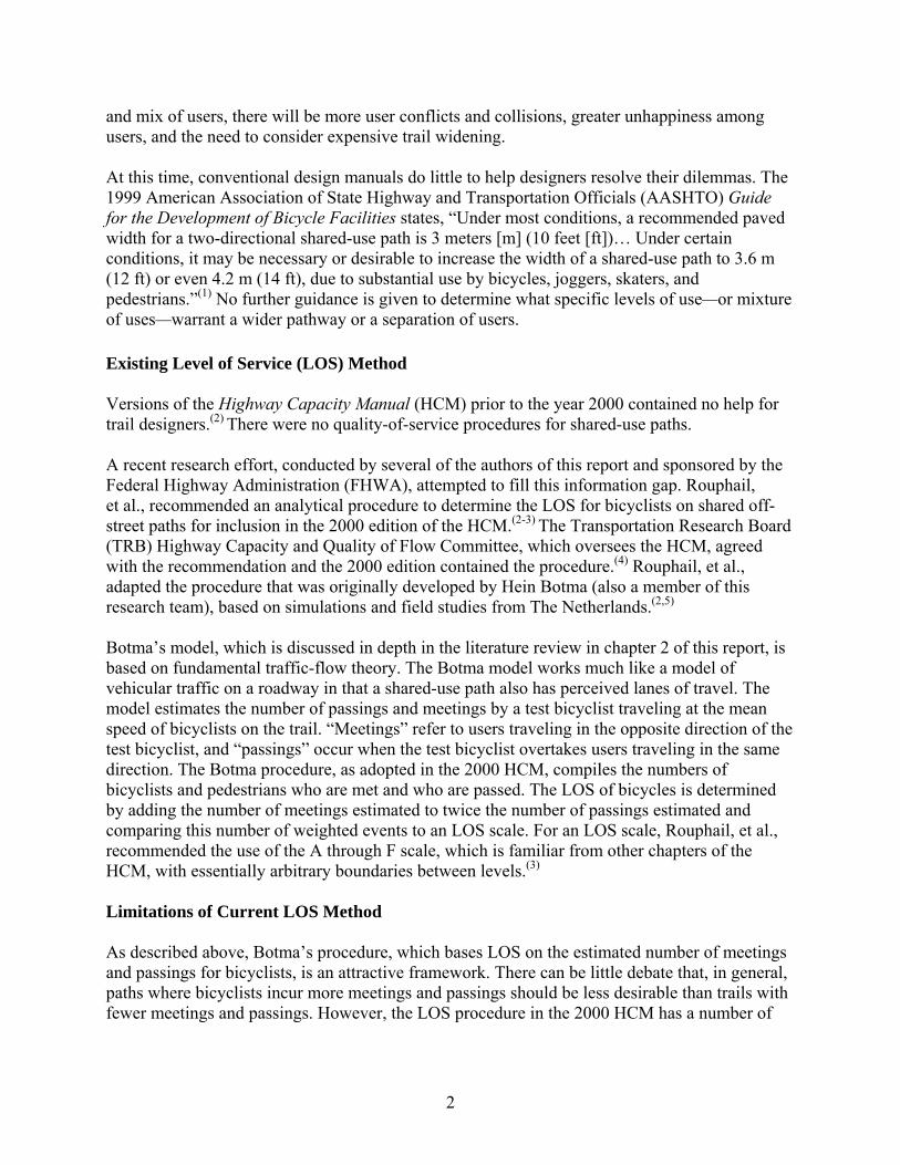
and mix of users, there will be more user conflicts and collisions, greater unhappiness among users, and the need to consider expensive trail widening. At this time, conventional design manuals do little to help designers resolve their dilemmas. The 1999 American Association of State Highway and Transportation Officials (AASHTO) Guide for the Development of Bicycle Facilities states, “Under most conditions, a recommended paved width for a two-directional shared-use path is 3 meters [m] (10 feet [ft])… Under certain conditions, it may be necessary or desirable to increase the width of a shared-use path to 3.6 m (12 ft) or even 4.2 m (14 ft), due to substantial use by bicycles, joggers, skaters, and pedestrians.”(1) No further guidance is given to determine what specific levels of use—or mixture of uses—warrant a wider pathway or a separation of users. Existing Level of Service (LOS) Method Versions of the Highway Capacity Manual (HCM) prior to the year 2000 contained no help for trail designers.(2) There were no quality-of-service procedures for shared-use paths.

A recent research effort, conducted by several of the authors of this report and sponsored by the Federal Highway Administration (FHWA), attempted to fill this information gap. Rouphail, et al., recommended an analytical procedure to determine the LOS for bicyclists on shared off-street paths for inclusion in the 2000 edition of the HCM.(2-3) The Transportation Research Board (TRB) Highway Capacity and Quality of Flow Committee, which oversees the HCM, agreed with the recommendation and the 2000 edition contained the procedure.(4) Rouphail, et al., adapted the procedure that was originally developed by Hein Botma (also a member of this research team), based on simulations and field studies from The Netherlands.(2,5) Botma’s model, which is discussed in depth in the literature review in chapter 2 of this report, is based on fundamental traffic-flow theory. The Botma model works much like a model of vehicular traffic on a roadway in that a shared-use path also has perceived lanes of travel. The model estimates the number of passings and meetings by a test bicyclist traveling at the mean speed of bicyclists on the trail. “Meetings” refer to users traveling in the opposite direction of the test bicyclist, and “passings” occur when the test bicyclist overtakes users traveling in the same direction. The Botma procedure, as adopted in the 2000 HCM, compiles the numbers of bicyclists and pedestrians who are met and who are passed. The LOS of bicycles is determined by adding the number of meetings estimated to twice the number of passings estimated and comparing this number of weighted events to an LOS scale. For an LOS scale, Rouphail, et al., recommended the use of the A through F scale, which is familiar from other chapters of the HCM, with essentially arbitrary boundaries between levels.(3) Limitations of Current LOS Method As described above, Botma’s procedure, which bases LOS on the estimated number of meetings and passings for bicyclists, is an attractive framework. There can be little debate that, in general, paths where bicyclists incur more meetings and passings should be less desirable than trails with fewer meetings and passings. However, the LOS procedure in the 2000 HCM has a number of

3

serious limitations that make it difficult for designers to use in resolving their path design dilemmas. These limitations include: • The procedure needs to be calibrated and validated for U.S. conditions. As detailed in

chapter 2, Botma’s equations are based on sound theory and they are based, in part, on field data from The Netherlands.(5) However, they have never been compared to U.S. field data. U.S. paths are typically wider than European paths. U.S. bicyclists are generally not as experienced. U.S. bicyclists tend to ride more often for recreation and less often for commuting. And U.S. bicycles are different from European bicycles. Among the parts of the model that need to be calibrated is the relative weighting of passings to meetings.

• The procedure does not account for “passive passings.” This is an event when the test

bicyclist is passed by a faster path user. Passive passings are probably undesirable from the test bicyclist’s perspective and should be considered in an LOS procedure.

• The procedure assumes that path users do not impede each other’s movements (i.e., that

there is always adequate room for the test bicyclist to pass with no change in speed or lateral positioning). This is true only if: (1) the path is wide enough, and/or (2) there is no opposing traffic during the passing maneuver. If passing is restricted, there will be a number of “delayed overtakings.” The significance of this limitation cannot be overstated. When passing and meeting become restricted, the procedure cannot predict that the LOS will worsen, because the number of events actually decreases. The procedure also assumes that bicyclists always want to pass any encountered bicyclists or pedestrians who are going at a slower rate. However, if the speed difference is small, or if the test bicyclist is near the end of his or her time on the path, this will not be true.

• The current LOS procedure for shared-use paths accounts for pedestrians and bicycles

only. However, in his original model, Botma simulated other path users, including mopeds and tandem bicycles.(5) Shared-use paths in the United States currently accommodate large numbers of joggers, inline skaters, skateboarders, and other types of users. The addition of other path users can be represented analytically in one of two ways. If a path user group appears to have a similar mean speed to another group, then such groups can be combined into one larger group that has a common mean and standard deviation. However, if a group is quite different from the others, then all events associated with this group must be estimated using separate equations.

• The current procedure is based on single values of mean bicycle and pedestrian speed.

Designers in areas where bicycles and pedestrians may travel faster or slower should have the ability to incorporate that information into their LOS estimates.

• The 2000 HCM method is limited to the analysis of two-lane and three-lane paths.

Furthermore, two-lane paths are specified as 2.44 m (8 ft) wide, and three-lane paths are specified as 3.05 m (10 ft) wide. Designers considering other widths and numbers of lanes have no current guidance.

4

• A stronger basis for the LOS criteria is clearly needed. While most of the LOS criteria in the 2000 HCM were set based on the expert opinion of the members of the Highway Capacity and Quality of Service Committee, there is recent research in some areas that bases the criteria on user surveys. In the pedestrian and bicycle arena, Harkey, et al., and Landis, et al., both members of this research team, have developed LOS criteria for on-street bicycle paths that are validated against user perceptions of the quality of service.(6-7)

A set of LOS criteria that is well grounded in user perceptions would be more credible than a set based on expert opinion alone.

• There is a great need to effectively convey the procedure and criteria to shared-use path

designers and operators. The HCM should certainly remain as one way to convey the procedure and criteria. However, the HCM is not a prominent document among shared-use path designers and operators. Also, the next version of the HCM may not be issued for many years. We need to convey any new procedure to the users in an effect manner and sooner.

With all of these limitations on the current LOS procedure, the need is clear for a substantial research effort to refine the method and to provide designers with a new procedure. PROJECT OBJECTIVE The overall project objective was the production of a tool that professionals can use to evaluate the operational effectiveness of a shared-use path, given a traffic forecast or observation at an existing path along with some geometric parameters. The project adopted Botma’s method as the basic framework for the LOS procedure.(5) In particular, the objective was to produce a tool that would overcome the major limitations in the current LOS procedure noted above. It was desirable that the procedure emerging from this project would: • Be calibrated and validated. • Be based on U.S. data. • Have LOS criteria based on user input for a typical mix of trip purposes. • Include more modes. • Include the ability to change key parameters such as mean speeds. • Account for delayed passing. • Analyze the full range of existing and possible path widths. • Be in a form ready for use by path designers. PROJECT METHODS The four major activities needed to achieve the project objective described were: 1. Development of the additional theoretical framework necessary to overcome the

limitations of the existing procedure noted above. 2. Collection of field data on path operations to calibrate and validate the theoretical

equations for U.S. conditions.

5

3. Collection of path user perception data to establish LOS criteria. 4. Development of an LOS estimation tool that professionals working with shared-use paths

could use, and a plan to distribute that tool. Development of Theory To achieve its objective, the project team had to develop the theory of traffic flow on shared-use paths in two important ways. First, the team had to determine a way to calculate the number of passive passings that occurred on a typical path. As noted above, a passive passing is an occasion when the test bicyclist is passed by a faster path user. Because bicyclists are typically the fastest users on a path, the number of passive passings is probably small in most cases; however, it should contribute to an LOS estimate. Passive passings were not used in the 2000 HCM procedure.

Furthermore, the team had to find a way to calculate the number of delayed passings. These are times when the test bicyclist would arrive behind a slower path user and not be able to pass because of the lack of an adequate-sized gap in the next lane to the left (oncoming or same direction). Obviously, delayed passings are undesirable for bicyclists since they would have to slow down and then expend energy accelerating when an adequate gap appears. Delayed passings are also critical because they are so closely related to path width. Prior to this project, there were some delayed passing calculations in the literature related to two-lane highway operation and similar facilities; however, nothing in the literature related to shared-path operation. Operational Data Collection The objective of the operational data collection portion of this project was to collect the field data needed to calibrate and validate the LOS model for shared-use paths. To calibrate and validate an LOS model, the main variables that needed to be collected were meetings and desired and actual passings by path users. Other data that need to be collected are the mean speed and speed range of the different user groups. In addition, trail characteristics must be recorded at each site. To ensure later flexibility, it was desirable that scenes on paths of interest be recorded from different perspectives so that additional data could be obtained by viewing videotapes if needed. The project proposal identified three methods of data collection: (1) a one-camera method, (2) a two-camera method, and (3) a moving-bicycle method. The one-camera method placed a camera at an elevated position where it could record scenes on a long path segment. The two-camera method recorded when path users entered and exited a path segment of interest, inferring meetings and passings on that segment. The moving-bicycle method, by contrast, collected meetings and passings from the perspective of a test bicyclist using a camera mounted on the bicyclist’s helmet. After careful consideration of all of the pros and cons for all three methods, the team chose to use the moving-bicycle method. Vantage points for the one-camera method would be rare (tall

6

buildings and hills with unobstructed views of qualifying shared-use paths are not common in the United States). The two-camera method would not be able to identify the difference between actual passings and desired passings because only path users would know whether they wanted to pass and were unable to do so and why. For example, a bicyclist may not have been able to pass because of inadequate path width or congestion. The moving-bicycle method can collect the needed data without these problems. The moving-bicycle method can be supplemented with a stationary camera on the side of the path. It can also be used to record path user volumes and the characteristics of different user groups, such as mean speed. Consequently, the moving-bicycle method, supplemented by a stationary camera, was the primary operational data collection method. Perceptual Data Collection A major part of this effort was to help set the LOS criteria by collecting data on user perceptions of multi-use trail design and operations. From a user perception standpoint, the intent of the present study was to quantify the effect of selected operational trail parameters on bicyclist and pedestrian judgments of the perceived adequacy of the trail facility. It is recognized that user responses will differ, depending on the individuals’ own reasons for using the trail (e.g., whether they were seeking a casual and relaxed activity or a rigorous individual workout unencumbered by users with more relaxed intentions). It was beyond the scope of this study to collect data on user perceptions as a function of users’ individual intentions or needs. However, an effort was made to obtain the opinions of a variety of users. The research team believed that it was possible to define the LOS for a trail in operational terms, independent of the factors governing the capacity of the trail. For example, a two-lane trail will obviously have less capacity than a four-lane trail; however, both, under different demand conditions, may be described as operating at the same LOS. In the present study, LOS is assumed to vary as a function of operational trail conditions that can be specified largely in terms of meeting and passing events. Depending upon the capacity of a trail and its particular level of use, each trail can be described in terms of the frequency of these meeting and passing events. If it could be shown that users’ judgments of the adequacy of a trail vary as a function of such events, it would be possible to predict user response to trail conditions and designs beyond the limited set of paths addressed by the study. A Usable Procedure As noted above, an important element of this project was that the procedure developed was usable by trail design professionals and that it would be distributed in a manner that would reach them. The research team included trail design professionals who carefully crafted the products for their colleagues. In addition, the researchers developed products that could be adopted in future versions of the HCM, as well as distributed in other ways. A section later in this chapter describes the research products in more detail.

7

PROJECT SCOPE LIMITED The scope of the project and, therefore, the products emerging from the project, was limited in several important ways. First, the project was limited to selected nonmotorized travel modes. We set out to expand the current procedure to those nonmotorized modes that are common on typical U.S. shared-use paths. In the end, we collected data on adult bicyclists, child bicyclists, walking pedestrians, running pedestrians, and inline skaters, and included these in our LOS method. Other modes of travel seen occasionally on shared-use paths, such as roller skaters, scooters, wheelchairs, Segways, and tandem bicycles, were not included because we did not see enough of them during our data collection for inclusion. Riders on horseback and snowmobiles are examples of other occasional path users that were outside the scope of this effort because they did not use the paths of interest in large numbers year-round. The LOS estimation procedure could be expanded to include any of these modes, or any other mode, if the analyst possessed some basic data about the mode, such as mean speed.

The scope of the project was also limited to off-street, paved paths. Although the methodology developed could apply to paths used exclusively by bicyclists and to one-way paths, the bulk of the attention in this research was centered on two-way paths serving pedestrians, bicyclists, and other users because they are the vast majority of the off-street paths in the United States. Since most paths with gravel, dirt, wood chips, or other loose material on the surface do not attract much bicycle volume, project data collection and analysis were limited to paths that were paved or had hard surfaces. A designer who is working on a path that has a hard-packed gravel or granular stone surface on which bicyclists operate in a very similar manner to paved paths may be able to apply the methodology we developed for that path with minimal additional error. Also, the project scope was limited in that the LOS produced was from the bicyclist’s point of view. The researchers collected some perception data from the pedestrian’s point of view, but not enough to establish their own LOS scale. Chapter 9 will recommend future research targeted at estimating path LOS from the points of view of pedestrians, skaters, and others. Furthermore, the project scope was limited to the analysis of trail segments at least 0.40 kilometers (km) (0.25 miles (mi)) long, uninterrupted by stop signs, signals, important intersections, or other similar features. Analysts will need other ways to find the LOS at these points. Finally, the project results were not intended for forecasting the number of future users of a path. While there may be some overlap between operational/design and forecasting methods, the premise behind this effort is that user volumes are an input rather than an output. The intent of this project was to answer questions regarding how wide the path should be to satisfy current or future demand, rather than to estimate how many users would be attracted to a path of a certain design.

8

RESEARCH PRODUCTS Description of the Products The three final products of this study are: (1) this report, (2) Share-Use Path Level of Service Calculator: A User’s Guide (User’s Guide) (Publication No. FHWA-HRT-05-138), and (3) Evaluation of Safety, Design, and Operation of Shared-Use Paths, a TechBrief (Publication No. FHWA-HRT-05-139). These products will be distributed primarily via the U.S. Department of Transportation (USDOT) Pedestrian and Bicycle Information Center (PBIC) Web site. The User’s Guide provides detailed, step-by-step instructions on how to use the LOS procedure and spreadsheet calculation tool, which can be downloaded from the Turner-Fairbank Highway Research Center Web site at www.tfhrc.gov. The User’s Guide and TechBrief can also be downloaded from the Web site. The widespread use and application of the LOS methodology is ultimately dependent upon how easy it is to use, whether it is considered applicable to trail design scenarios, and whether trail designers are able to gather the data needed to use the model. At this time, there are two main applications of the model: (1) to determine the appropriate width of a new trail, and (2) to determine how much width to add to an existing trail to accommodate current or projected levels of use. Determining whether to separate modes or directions of travel is also emerging as a key application. The availability of data and its ease of collection are often key components in the success of an LOS model. We tried to ensure that the data items collected for the model would be relatively easy for a trail designer to obtain. We also recommended default values for most of the needed inputs. In addition, the User’s Guide describes how to effectively collect data for use in the model. Our idea for the LOS calculator was that it should be some type of spreadsheet application or self-executing graphical user interface software. The team was inspired by the League of Illinois Bicyclists, which developed online graphical user interface software that calculates a bicycle LOS for a roadway using the Bicycle Compatibility Index and the Bicycle LOS model (see http://www.bikelib.org/roads/blos/losform.htm).(6-7) The interface is easy to use, is accessible directly from the League’s Web site, and suggests default values if an analyst does not have all of the necessary data. A user can simply click on the calculate button, and an LOS result for each model is displayed. We attempted to create a calculator for our shared-use path LOS model that would be made available in a similar format and would allow users to easily calculate an LOS for a shared-use path. Intended Users Unlike the roadway environment, which is almost exclusively the domain of civil engineers, shared-use paths are designed by a wide variety of practitioners. Some of the most creative and unique trails in the country are the direct result of the diverse skills of these designers. Since

9

these professionals look to a variety of different sources for design guidance, establishing national guidelines is difficult. We identified three main target audiences for the marketing of our shared-use path LOS model: (1) transportation professionals, (2) trail designers/coordinators, and (3) pedestrian, bicycle, and trail advocates and organizations: • Transportation Professionals. These individuals are engineers, planners, or designers.

They work in planning, engineering, and public works departments at all levels of government. They may also work for consulting firms or at research institutes. These individuals often rely on roadway design manuals such as the AASHTO Guide for the Development of Bicycle Facilities, the Highway Capacity Manual, the AASHTO Policy on Geometric Design of Highways and Streets (the Green Book), and the Manual on Uniform Traffic Control Devices (MUTCD), along with other State and local roadway design manuals. (See references 1, 4, 8, and 9.) Transportation professionals are more likely to possess a technical background in standard LOS applications, roadway cross sections, and in the design of roadways and/or bicycle and pedestrian facilities.

• Trail Designers/Coordinators. These individuals are planners, landscape architects, or

other professionals who are involved in the design, development, and maintenance of trails; however, they may not have a technical background in transportation planning. They work in planning, parks and recreation, environmental protection, or greenway and trail departments at all levels of government, and they also may be consultants hired by governments to design shared-use paths. They often rely on park and recreation design manuals, information about the design of trails obtained from various clearinghouses, and past professional experience. This group is important to reach because they often make decisions about the design, location, and development of shared-use paths.

• Pedestrian, Bicycle, and Trail Advocates and Organizations. These groups often play

an essential role in making shared-use paths a reality. Organizations such as Rails-to-Trails Conservancy and East Coast Greenway Alliance often provide technical guidance and/or serve as clearinghouses for innovative design approaches. Local trail alliance/advocacy groups are often influential, and many times they make major decisions in the development of shared-use paths. It is important that the shared-use path LOS model address their concerns and that it be embraced as a useful tool by these groups as well. These groups frequently set a vision for trails in a community, provide input into the kinds of trails to be created, and provide coordination among the many players who will develop, own, and manage the trail.

Through this report, the User’s Guide, and the TechBrief, we tried to reach all three of these groups. It should be noted, however, that the primary intent of this report is to provide technical details with regard to our methods and data. Unlike the User’s Guide and the TechBrief, this report is not intended for wide distribution.

10

REPORT FORMAT This report includes eight chapters in addition to the introductory chapter. Chapter 2 is a review of the literature pertaining to LOS estimation for shared-use paths. Chapter 3 describes the development of the theoretical background that we needed for the procedure. Chapter 4 discusses the methods we used to collect the field data on path operations. Chapter 5 shows how we used the field data to calibrate and validate our LOS model. Chapter 6 describes how we collected data on user perception of shared-use paths having various geometric and operational characteristics. Chapter 7 shows how we analyzed the perception data in order to develop the LOS criteria. Chapter 8 presents the highlights from the LOS procedure. (A much more comprehensive guide to the procedure, written for the audiences we described above, is available in the User’s Guide.) Finally, chapter 9 provides a summary of the project and our recommendations for future research to improve technical capabilities in this area. At the end of the report are a set of appendixes and a complete list of references.

11

2. LITERATURE REVIEW

INTRODUCTION This chapter provides a thorough, critical review of the major, relevant research to date on the topic of LOS estimation for shared-use paths. The chapter contains sections on path user characteristics, ways to measure the quality of the performance of the shared path for the users, and ways to establish an LOS scale. The review will indicate why path designers and others needed a research project on this topic, and will show which directions the project had to take. Much of the material in this document is from previous recent work by members of the project team for the FHWA, including Rouphail, et al.,(10) and Allen, et al.(11) The document also includes results from searches of computerized indexes and manual searches by the project team of available library resources. PATH USER CHARACTERISTICS Pedestrian Characteristics There is a wide variety of users within the pedestrian population and, therefore, a large variety of needs within this population that have to be addressed by path designers. One can classify pedestrians by gender, age, or trip purpose, among other typologies. In addition, disabled pedestrians have unique requirements that the profession must address in order to adequately serve this group. Gender is an important factor where pedestrians are concerned. Fruin notes that despite the consistency in walking gait across both sexes and all ages, differences in other aspects of pedestrian walking and standing exist among these groups.(12) For example, adult male pedestrians consume more area than their female counterparts, and female pedestrians exhibit a higher level of pelvic rotation for a given length of stride. Polis, et al., observed differences in walking speeds between male and female pedestrians in Israel.(13) The authors attributed this primarily to the typically greater physical size and stride of males; they also noted a second hypothesis—that a greater number of males than females were walking to and from work in Israel. Another dividing factor is age. Aging reduces the length of the stride of a pedestrian and results in a commensurate reduction in walking speed.(12) Very young pedestrians will also walk at a slower gait than other groups.(14) There may also be differences between pedestrians of different ages, including perception, reaction time, and risk-taking, which are important considerations in evaluating passing, although there has been limited attention paid to these aspects in the pedestrian literature. Knoblauch, et al., note that the current traffic environment is “not well adapted to the needs of the older pedestrian” and reports that older pedestrians have the highest pedestrian fatality rate of any age group.(15) With decreases in visual acuity accelerating after age 60, and with reductions

12

in walking speeds prevalent among the elderly, the transportation professional faces unique challenges in attempting to service this segment of the population. One can also divide pedestrians into groups by trip purpose. Commuting pedestrians exhibit higher pedestrian speeds than do shoppers.(16) By stopping to window-shop, the latter group also consumes more of the walkway width.(16) Students exhibit different characteristics than other groups.(17) Impaired users are a critical concern for the designers of pedestrian facilities. In a recent report for FHWA, Kirschbaum, et al.,(18) describe many different types of users who the designers of pedestrian facilities should consider, including: • Stroller users. • Wheelchair users. • Individuals with limited balance. • Individuals with a vision impairment. • Older adults. • Children. • Individuals who are obese. • Crutch or support cane users. • Individuals with low fitness levels. • Individuals with cognitive impairments. • Individuals with emotional impairments. Kirschbaum, et al., cite Census Bureau statistics from 1994 that “approximately 20 percent of Americans have a disability and the percentage of people with disabilities is increasing.”(18) In terms of pedestrian space requirements, designers of pedestrian facilities (considering only unimpaired pedestrians) use body depth and shoulder breadth, at least implicitly, for minimum space standards. In addition, pedestrians require a certain minimum space for comfort. Fruin described these concepts as the “body ellipse” and the “body buffer zone.”(12) All recent editions of the HCM applied the concepts of pedestrian space as a measure of effectiveness with regard to pedestrian facility analysis procedures. (See references 2, 4, 14, and 19.) As noted by Tanaboriboon and Guyano, cultural attitudes and prevailing pedestrian characteristics may affect space requirements.(20) For example, they note that Asians are typically smaller than Westerners, and that Asian pedestrians require less personal space than Americans. Fruin notes that the average adult male body occupies an area of about 0.14 square meters (m2) (1.5 square feet (ft2)).(12) Given the existence of body sway in both idle and moving persons, as well as the typical preference to avoid contact with others, Fruin presents the concept of a 45.7-centimeter (cm) by 61.0-cm (18-inch by 24-inch) body ellipse, with a total area of 0.279 m2

(3 ft2), as the practical minimum standing area. Davis and Braaksma use a similar body ellipse of 46.0 cm by 61.0 cm (18 inches by 24 inches) in their study of Canadian transportation terminals.(21)

13

Pushkarev and Zupan note that pedestrians can occupy as little as 0.09 m2 (0.97 ft2) per woman and 0.14 m2 (1.50 ft2) per man, but require about 0.22 to 0.26 m2 (2.4 to 2.8 ft2) per person to avoid touching, and prefer a body buffer zone of 0.27 to 0.84 m2 (2.9 to 9.0 ft2) to avoid “emotional discomfort in the presence of strangers.” Flow involving “unnatural shuffling” begins when space falls below 0.75 m2 (8.1 ft2).(22) Navin and Wheeler(23) state that an individual’s “domain” (clear space around the individual) could be defined by a parabolic curve with its apex about 0.75 m (2.4 ft) in front of the pedestrian and the edges about 0.40 m (1.3 ft) to the pedestrian’s sides. There is little information in the technical literature on joggers on shared-use paths. Most of the recreational literature on joggers relates to optimizing performance rather than characterizing typical joggers. Bicyclist Characteristics There are estimated to be more than 100 million bicyclists in the United States; however, less than 1 percent of travel trips are made by bicycling in this country.(24) According to one source, there are three general categories of bicycle users: (1) the child bicyclist, (2) the casual or inexperienced adult bicyclist, and (3) the experienced adult bicyclist.(25) A report released by FHWA divides bicyclists into three similar categories: (1) Group A: Advanced Bicyclists, (2) Group B: Basic Bicyclists, and (3) Group C: Children.(26) The behavior and attributes of these three groups differ; however, most bicycle facilities cater to all three types of bicyclists. The child bicyclist (group C) is defined as a bicyclist who is too young to obtain a motor vehicle operator’s license (age 16 in most States). Approximately three-quarters of all children under age 16 ride bicycles, and this group makes up a little less than half of all bicyclists.(25) A high percentage of children are forced to ride bicycles because they have no other transportation alternatives. This group tends to prefer residential streets with low motor vehicle speed limits and volumes, well-defined bicycle lanes on arterials and collectors, and/or separate bicycle paths. The casual or inexperienced adult bicyclist (group B) is defined as someone who is old enough to possess a motor vehicle operator’s license, is moderately skilled, and has a basic, but not extensive, knowledge of bicycling. For this group, bicycling is mostly a recreational activity that is done on residential streets and bicycle paths. However, this group occasionally will make purposeful trips and/or use major streets. It is estimated that this group makes up approximately 40 percent of the overall bicycling population.(25) The experienced or advanced adult bicyclist (group A) is defined as an experienced, knowledgeable, and skilled bicyclist who is old enough to possess a motor vehicle operator’s license. This group tends to use the bicycle for longer trips and more often for purposeful trips than the casual adult bicyclist. It is estimated that this group makes up approximately 10 percent of the overall bicycling population.(25) This group normally prefers to use the most direct route to its destination, and riders are willing to use a variety of different types of streets with or without designated bicycle facilities.

14

FHWA reports that more than 50 percent of bicycle trips in the United States are taken for social/recreational purposes.(24) The other trip categories were personal or family business, school and church, work, and “other” trips. Bicycle trips are often divided into just two categories for operational analysis: (1) recreational trips and (2) purposeful trips. Purposeful trips include all categories other than social/recreational. The fact that more than half of all bicycling trips may be recreational must be considered when analyzing bicycle traffic, because the same is generally not true for motor vehicles. Hunter, et al., conducted a study in several U.S. cities and found that bicycle traffic volumes between the hours of 7 a.m. and 7 p.m. on weekdays were fairly constant, with peak-hour volumes being approximately 1⅓ times the average hourly volumes.(27) They also found that the peak hours on weekdays typically corresponded with local commuter schedules. In one city, they measured peak-hour volumes as 10 to 15 percent of total daily volume. The proportion of weekday to weekend traffic varied greatly, depending on the recreational uses of the bicycle facilities. Seasonally, they found that volumes were generally highest in the summer and lowest in the winter. A study conducted in the Seattle area by Niemeier analyzed bicycle volume data collected over 1 year at five separate locations.(28) The study showed that bicycle volumes were higher during the p.m. peak than during the morning peak at all but one location, which was slightly lower. Three of the locations had more than double the volume during the p.m. peak. Bicycle peak-hour factors (PHFs) between 0.52 and 0.82 were observed during the morning peaks at the various locations, and PHFs between 0.58 and 0.80 were observed during the p.m. peaks. The study showed significant variability in volumes over the year. This variability suggested that a single volume count could be biased by as much as ±15 percent, depending on the time of year that the count was taken. Volumes were much lower during adverse weather because bicyclists are exposed to the elements. Because of the recreational and social nature of bicycling, bicycle users often ride in pairs. A study found that in The Netherlands, the number of paired bicycles was a function of bicycle volume.(5) However, the dependence differed with location. As expected, the study also found that paired riding was more common during recreational bicycle trips than purposeful trips. The fact that bicycle users often ride in pairs has been noted by others; however, no other attempt has been made to quantify this phenomenon. Other than the bicyclists, the bicycle itself has known properties that have to be taken into account. With regard to space requirements, a typical bicycle in the United States is 1.75 m (5.75 ft) in length, with a handlebar width of 0.60 m (2 ft).(25) In The Netherlands, it has been reported that 95 percent of bicycles are less than 1.90 m (6.25 ft) in length and that 100 percent of bicycle handlebar widths are less than 0.75 m (2.5 ft). In addition, a bicyclist needs a certain amount of operating space. No bicyclist, at any speed, can ride a bicycle in a perfectly straight line. One U.S. source reports that a typical bicycle needs between 0.75 m (2.5 ft) and 1.40 m (4.5 ft) of width in which to operate.(25) This amount of space can also be referred to as the effective lane width for a bicycle. An older study in Davis, CA, recommends a minimum width of 1.28 m (4.2 ft) for bicycles, with additional width at higher

15

volumes.(29) In The Netherlands, 1.00 m (3.3 ft) of clear space is generally recommended for bicycles.(30) In Germany, 1.00 m (3.3 ft) is reported as the normal width of one bicycle lane.(31) In Sweden, 1.20 m (3.95 ft) is reported as a typical bicycle lane width.(32) A Chinese study reports that the width of a two-lane bicycle path in China is generally 2.5 m (8.2 ft), with an additional 1.0 m (3.3 ft) added for each additional lane.(33) The Norwegian Public Roads Administration states, “One meter is not enough,” and recommends a width of 1.6 m (5.3 ft) for single-lane bicycle lanes.(34) Overall space requirements for bicycles can also be defined in terms of density. A Canadian study found that bicycle operating space greater than 9.3 m2/bicycle (100.1 ft2/bicycle) provided for free-flow bicycling conditions.(35) The study also found that when less than 3.0 m2/bicycle (32.3 ft2/bicycle) of operating space is provided, there was no freedom for bicycles to maneuver. A study in China(33) found that bicycle operating space greater than 10 m2/bicycle (107.6 ft2/bicycle) provided very comfortable operations, and that less than 2.2 m2/bicycle (23.7 ft2/bicycle) forced most cyclists to dismount and walk their bicycles. The older study in Davis, CA, found that bicycle operating space greater than 20 m2/bicycle (200 ft2/bicycle) provided free-flow conditions and that less than 3.7 m2/bicycle (40 ft2/bicycle) represented congestion.(36) Free-flow speed is also important in the study of bicycle operations. The Davis, CA, study reported a mean velocity of approximately 19 kilometers per hour (km/h) (11.8 miles per hour (mi/h)) for class I bicycle facilities and mean bicycle velocities between approximately 17.7 km/h (11.0 mi/h) to 20.1 km/h (12.5 mi/h) for class II facilities.(29) Class I facilities are off-street paths and class II facilities are designated as on-street bicycle lanes. Another study conducted in Davis, CA, reports that the free-flow speed of bicycles is usually above 17.7 km/h (11.0 mi/h).(36) A study conducted primarily in Michigan on university campuses reported average observed speeds of 24.9 km/h (15.5 mi/h) on bicycle lanes and 20.3 km/h (12.6 mi/h) on bicycle paths.(37) A manual released by FHWA(38) reported that the 85th percentile speed of bicycles is approximately 24 km/h (15 mi/h), and that a design speed of 32 km/h (20 mi/h) on level terrain would allow for nearly all bicyclists to travel at their desired speeds. In Sweden, the 85th percentile free-flow speed of bicycles is reported to be between 16 km/h (10 mi/h) and 28 km/h (17.4 mi/h).(32) A Canadian study found a free-flow speed of 25 km/h (15.5 mi/h).(35) One study in China reported observed average bicycle speeds at various locations between 10 km/h (6.2 mi/h) and 16 km/h (10 mi/h), with an overall mean of approximately 12 km/h (7.5 mi/h).(39) Another Chinese study reported observed average bicycle speeds between 12 km/h (7.5 mi/h) and 16.3 km/h (10.1 mi/h), with an overall mean of approximately 14 km/h (8.7 mi/h).(40) A more recent Chinese study reported peak-hour free-flow speeds of 18.2 km/h (11.3 mi/h), where bicycle traffic was separated from motor vehicles by a barrier, and 13.9 km/h (8.6 mi/h) at locations without a lane barrier.(41) A Dutch study reported a mean bicycle speed of 18 km/h (11.2 mi/h), with a standard deviation of 3 km/h (1.9 mi/h).(42) The Dutch study also reported that the observed average speed appeared to be unaffected by path width.

16

Virkler and Balasubramanian(43) conducted the most detailed field study on shared-use paths using North American data collected prior to this study. Their study focused on operational data collected along two multi-use facilities (one in Columbia, MO, and the other in Brisbane, Australia). Mean speeds were recorded for hikers, joggers, and bicyclists. Results from the speed study showed that the mean speed of joggers was roughly twice that of hikers, and the mean speed of bicyclists was roughly twice that of joggers. As expected, the standard deviation of speed within each user group increased as the mean speed increased. The mean speeds collected at the Missouri site were similar to those collected at the Brisbane site; however, the standard deviation of speeds was much higher at the Missouri site for the jogger and bicyclist user groups. In addition, passing data for each user-group combination were collected at the two sites. Passing data recorded at the two sites showed significant differences with respect to the mean passing time. On average, passing times at the Columbia site were approximately twice as long as passing times at the Brisbane site. This is to be expected given the larger standard deviation of speeds observed at the Missouri site. A total of 206 passing maneuvers were recorded at the Brisbane site compared to 49 passing maneuvers at the Columbia site.

In an earlier effort, Botma and Papendrecht(5) collected operational data on four paths within a town and on one tour (race) path outside of town. The narrowest town path was 1.8 m wide, while the other three were approximately 2.5 m (8.2 ft) wide. The paths selected for the data collection contained only bicycle and moped traffic. No pedestrians were observed. Speed and lateral clearance data were collected for all bicycles and mopeds. Passing data (i.e., frequency, passing time, and lateral clearance) were also collected. The average bicycle speed recorded at each of the sites was 19 km/h (11.8 mi/h), which is comparable to Virkler and Balasubramanian’s observations.(43) However, the standard deviation found by Botma and Papendrecht (4.8 km/h (3 mi/h)) was much lower than that found by Virkler and Balasubramanian (4.8 to 7.6 km/h (3 to 4.7 mi/h)).(5,43) Interestingly, curb height, which varied from 3 to 10 cm (1.1 to 3.9 inches), did not affect the lateral position of bicyclists; however, it did affect that of mopeds. Bicycle passing data collected in this study indicate that on the narrower 1.8-m path, the distance over which passing occurred was quite short (about 24 m (79 ft)) and took less than 5 seconds (s). On the 2.5-m path, passing took place over a much longer distance (about 63 m (206 ft)) and consumed more than 11 s. Therefore, based on this study, it appears that the wider paths provided a more comfortable transition for passing maneuvers as cyclists became less concerned about negotiating opposing traffic. In summary, we know a good deal about bicyclist characteristics, although there is a rather large range for some key parameters. For example, free-flow bicycle speed appears to be somewhere between 10 km/h (6.2 mi/h) and 28 km/h (17.4 mi/h), with a majority of the observations being between 12 km/h (7.5 mi/h) and 20 km/h (12.4 mi/h). Meanwhile, the design speed recommended by AASHTO for bicycle facilities in the United States is 32 km/h (20 mi/h), which is the same as that recommended by FHWA.(1) Other Path Users Bicyclists and pedestrians are typically not the only regular users of shared-use paths in the United States. Until recently, there has not been any significant quantitative research completed

17

in the United States that addresses the effects that other path users (i.e., inline skaters, skateboarders, scooters, etc.) have on the performance of the path. This changed with the recent publication of a final report from FHWA on the characteristics of many of these other path users.(44) The research team studied the characteristics of 811 users of 14 emerging devices in three States. They measured the physical dimensions of the devices, the space required for a three-point turn, the lateral operating space (sweep width), turning radii, acceleration capabilities, speed, and stopping sight distances. One of their most important findings that relates to the objectives of this study was that inline skaters had a sweep width of 1.5 m (5 ft). This is larger than the minimum bicycle lane width of 1.2 m (4 ft) recommended by AASHTO.(1) The team also found that for horizontal curve radius and stopping sight distance, the emerging devices that had the highest values were recumbent bicycles. Segways were included among the emerging devices studies during this effort, incidentally; however, the team found that Segway users would not be the critical users for any of the design criteria evaluated. In Europe, interest is rising in the role played by skaters on shared-use paths. The main concern seems to be safety, especially in city centers. Most of the current expressions of this concern are to blame the skaters and admonish them to behave better. There is no new information about adequate facilities that would incorporate skaters with other users. In fact, some observers believe that the number of inline skaters will rise in the short term, but will stabilize or fall in the medium and long term. MEASURING PATH USER QUALITY OF SERVICE Hindrance On shared-use facilities, the presence of pedestrians can be detrimental to bicycle quality of service because pedestrians move at much lower speeds. However, it is very difficult to establish a single bicycle/pedestrian equivalent value because the relationship between the two modes differs depending on their respective volumes, directional splits, and other conditions. Botma developed the concept of hindrance on shared-use paths to overcome this difficulty and to allow a meaningful quality of service to be computed.(42) Botma’s procedure for determining bicyclist LOS on a shared-use path is founded on the concept of the hindrance experienced by path users as they travel a unit length of the path.(42) Based on earlier field studies conducted at four sites in The Netherlands, he found that the correlation between bicycle volume and speed was very weak (R2 = 0.20).(5) Density, the ratio of volume and speed, has been used in Germany as the LOS indicator on trails; however, the selection of densities to delineate LOS can be rather subjective. Botma therefore concluded that LOS for bicycle paths should not be based on speed or density, but rather on the freedom to maneuver and the ability to make unrestricted passing maneuvers.(42) Hindrance reflects the degree to which a user is restricted from the freedom to maneuver. Such restrictions occur when a bicyclist passes a slower bicyclist or a pedestrian, or when he or she meets a bicyclist or pedestrian traveling in the opposite direction. LOS is then defined on the basis of the fraction of the path users that experience hindrance. For example, LOS A is said to occur when fewer than 10 percent of all users experience hindrance over a 1-km (0.62-mi) path.

18

On the other extreme, the LOS E/F boundary is reached when all users experience hindrance and when the average path user is expending about two-thirds of his or her time maneuvering around other users. It is important to note that the LOS E/F boundary occurs well before the path capacity is reached. Capacity in one lane on a bicycle path has been reported to be somewhere between 1,500 and 5,000 bicycles per hour, as will be shown later. Using a simple simulation model, Botma and Papendrecht were able to relate the percentage of hindrance to directional volumes.(45) Furthermore, because hindrance is difficult to measure directly in the field, the frequency of meeting and passing events was used as a proxy variable for hindrance. Of course, the conversion from events to hindrance requires some judgment about the “relative impedance” of each event from the user perspective. Since there was no guidance in the literature, Botma assumed that all meeting events are half as severe as all passing events.(42)

Therefore, the total hindrance is calculated as the weighted frequency of all meeting and passing events. The computation of the various event-type frequencies is described next. From the bicyclist’s perspective, the number of events experienced by the average bicyclist depends on: (1) whether the path is one way or two way, (2) whether the path is exclusive (bicycles only) or shared (bicycles, pedestrians, inline skaters, etc.), and (3) the directional volumes of all path users. For a two-way shared-use path serving primarily bicycles and pedestrians, there are four types of events, including: A. Bicycle passing a bicycle. B. Bicycle passing a pedestrian. C. Bicycle meeting a bicycle. D. Bicycle meeting a pedestrian. For case A, assume that bicyclists do not impede each other and that bicycle speeds are normally distributed with mean (Ub) and standard deviation (σb). The desired frequency of passing events (per hour and unit length) experienced by the average bicyclist in a directional bicycle flow of Qb per hour can be estimated:(46)

πσ

b

bb

UQ

AF2

)( = (1)

For case B, the frequency of pedestrians that the average bicyclist passes, assuming a directional pedestrian flow of Qp per hour with mean speed Up, is estimated by the following equation:

)1()(b

pp U

UQBF −=

(2) In case C, the frequency of opposing bicycles that the average bicyclist meets, assuming an opposing bicycle flow of Qbo, with mean speed Ubo, is estimated as:

19

(3)

In the event that the mean bicycle speeds are equal in both directions, F(C) simplifies to 2Qbo. Finally, for case D, the frequency of opposing pedestrians that the average bicyclist meets, assuming an opposing pedestrian flow of Qpo, with mean speed Upo, is estimated as:

)1()(po

bpo U

UQDF +=

(4) From the pedestrian’s perspective, Botma’s method assumes (probably unrealistically) that pedestrians do not impede each other on a shared-use path. Therefore, the relevant events are only those involving the interactions of pedestrians and bicycles. For a two-way, shared-use path that serves primarily bicycles and pedestrians, there are two such events (making the reasonable assumption that pedestrians never pass bicyclists): E. Pedestrian overtaken by bicycles traveling in the same direction. F. Pedestrian meeting bicycles traveling in the opposite direction. For case E, the hourly frequency of bicycles passing the average pedestrian on the path, assuming a directional bicycle flow of Qb per hour, and assuming pedestrian and bicycle mean speeds of Up and Ub, respectively, is estimated from:

)1()(b

pb U

UQEF −=

(5) In case F, the hourly frequency of opposing bicycles meeting an average pedestrian on the path, assuming an opposing directional bicycle flow of Qbo per hour, and assuming pedestrian and opposing bicycle mean speeds of Up and Ubo, respectively, is estimated from:

)1()(bo

pob U

UQFF +=

(6) A path-wide hindrance or LOS can be obtained by adding all the “impedance weighted” events for each path user, and then calculating the path average using the volume for all path users. The procedure reveals a high sensitivity of bicycle LOS to pedestrian volumes and a much lower sensitivity of pedestrian LOS to bicycle volumes. The two examples in table 1, taken from Botma, illustrate the point.(42) The LOS indicated in parentheses is the one predicted if the path were to be used exclusively by pedestrians or bicycles.

)1()(bo

bbo U

UQCF +=

20

Table 1. LOS examples for a two-way, shared-use path. Ex. Two-way,

pedestrians/h Two-way, bicycles/h

LOS-Ped

LOS-Bicycle

LOS-Combined

1

40

200

A (A)

F (D)

F

2

200

40

A (A)

F (A)

D

*Assuming a 50/50 split for all volumes. Until very recently, the HCM had no substantive material on bicycle operations and much less on shared-use paths.(2,14,19) Based on previous research performed for FHWA by some members of this research team, much of Botma’s work on shared-use paths (modified for U.S. conditions) was incorporated into the 2000 HCM.(3-4,7) This material appears in three chapters. Chapter 11 deals with pedestrian and bicycle concepts and provides descriptive information on the various facility types. Chapter 18 on pedestrians presents the effects of bicycles on pedestrian LOS on shared-use paths. Finally, chapter 19 on bicycles provides the most comprehensive treatment of shared-use paths. Analysis methods are provided for any combination of pedestrians and bicycles for one-way and two-way paths, and for two-lane and three-lane paths. Examples illustrating the LOS benefits of separating pedestrians and bicycles are provided. All of this material was reflected in the Highway Capacity software and in other software replicating HCM calculations. The one published effort to date that attempted to validate Botma’s method was by Virkler and Balasubramanian.(43) The bicycle passing data they collected on a shared-use path in Brisbane, Australia, were compared to predictions calculated using Botma’s hindrance models. The mean speed and standard deviation data from the Brisbane site were applied to Botma’s overtaking frequency model and were compared to the actual observations for each six passing combinations: (1) bicycle passing bicycle, (2) jogger passing jogger, (3) hiker passing hiker, (4) bicycle passing jogger, (5) bicycle passing hiker, and (6) jogger passing hiker. Results from the prediction model were very similar to the actual observations for all passing combinations, with the exception of the hiker passing hiker and jogger passing hiker combinations. The predicted frequencies for these two passing types were much higher than those observed in the field. Similarly, the predicted delayed overtakings for these two passing combinations were much higher than the actual delayed overtakings, while the rest of the combinations were quite comparable. Density Density has often been proposed as a measure of effectiveness (MOE) for bicycle facilities. Previous studies in California, (36) Germany,(31) and China(33) all proposed levels of service based on density. The California study reported that bicycle capacity occurs at approximately 2,600 bicycles per hour per 1.0-m (3.3-ft) lane. That study proposed that LOS A was at a density greater than 20 m2/bicycle (215 ft2/bicycle) while LOS F was at a density less than 3.7 m2/bicycle (40 ft2/bicycle). The German study proposed that LOS A was at a density greater than 200 m2/bicycle (2150 ft2/bicycle) while LOS F was at a density less than 10 m2/bicycle (108 ft2/bicycle). Instead of LOS of an A through F scale, the Chinese study proposed the following seven “states of bicycle traffic”:

21

• Very comfortable. • Comfortable. • Cannot overtake. • More dense. • Very crowded. • Prepare to dismount. • Dismount. The highest state, very comfortable, was at a density greater than 10 m2/bicycle (108 ft2/bicycle) while lowest state, dismount, was at a density less than 2.2 m2/bicycle (24 ft2/bicycle). Note that a density just over 10 m2/bicycle (108 ft2/bicycle) would produce an LOS E in Germany and would produce a “very comfortable” rating on the Chinese scale. No capacities were reported in the Chinese study. However, based on the speeds and densities reported, it appears that the capacity for a 2-m- (6.6-ft-) wide path is between 4,400 and 4,500 bicycles per hour, and the capacity of a 3-m- (9.9-ft-) wide path is between 6,600 and 6,700 bicycles per hour. Space The 2000 HCM uses space (m2/ped) as the primary measurement of effectiveness for pedestrian LOS on uninterrupted facilities.(4) The HCM uses that measurement because space dictates the pedestrians’ ease, speed, and freedom of movement. Because pedestrian movements are affected by the presence and relative location of other pedestrians, space is a viable measurement. Stress There are many components to the bicycling environment that need to be considered when thinking about the potential attractiveness of a bicycle facility or determining the best locations for new construction and improvements that would benefit bicycles. Researchers have identified many of those factors and have shown how they can help estimate the quality of service for a facility. To this point, such work has applied only to on-street bicycle facilities. Based on other studies, Northwestern University(25) has assigned stress levels between 1 and 5 to three primary factors and to three secondary factors that contribute to the relative attractiveness of an on-street bicycle facility. Level 5 suggests a high level of stress, and level 1 suggests a low level of stress. The assignment of an overall stress level to a facility is based on an average of the values for the three primary factors: • Motor vehicle volume in the adjacent lane. • Curb lane width in meters or feet. • Speed of the motor vehicles in the adjacent lane. Stress level 1 is associated with motor vehicle volumes of 50 vehicles per hour per lane, curb lane widths of 4.6 meters (15 feet), and motor vehicle speeds of 40 km/h (25 mi/h). Meanwhile, stress level 5 is associated with motor vehicle volumes of 450 vehicles per hour per lane, curb lane widths of 3.4 meters (11 feet), and motor vehicle speeds of 72 km/h (45 mi/h).

22

After the average of the three primary factors is found, the stress level of the facility can be subjectively rated based on the values of three specified secondary factors or on any other secondary factors that are felt to be important. The three specified secondary factors were: • Driveways per kilometer or per mile. • Percentage of heavy vehicles. • Parking turnover per hour per block. Stress level 1 is associated with 5 percent heavy vehicles, 6 driveways per kilometer (10 driveways per mile), and no parking allowed. Stress level 5 is associated with 15 percent heavy vehicles, 31 driveways per kilometer (50 driveways per mile), and 20 parking movements per hour per block. Other secondary factors mentioned for possible consideration include bicycle volume, pavement condition, sight distance, bus routes, presence of drainage grates, intersection turning volumes, and street grade. If an analyst felt that one or more of these additional secondary factors were important, a subjective decision could be made as to the degradation contributed to the stress level of the facility. Several local and State transportation agencies have developed their own stress level methods for on-street bicycle facilities. These are generally based on or look very similar to the Northwestern University method described above, using similar primary and secondary factors with slightly different values. SIMULATION MODELS Analysts could obtain performance measures on shared-use paths from computer simulation models. However, to date, there is no widely used computer simulation software in the United States that is capable of describing user interactions on shared-use paths in a realistic manner. The earliest attempt was a numerical, microscopic simulation model by Botma and Papendrecht.(45) The model included three types of users: solo bicyclists, bicyclists riding in pairs, and mopeds (no pedestrians). It is essentially a Monte Carlo simulator of individual entities whose speeds follow the normal distribution with exponentially distributed headway. The model assumes no impedance between users and is used to capture the number of passing and meeting events of various users for a variety of volume and speed ranges. Given that much of the model outputs are already captured by Botma’s analytical equations, the utility of such a model is questionable. There are obvious similarities between operations of nonmotorized traffic on shared-use paths, and motorized traffic on two-lane highways. Both facilities experience passing and meeting events, delayed passing, and conflicts with opposing traffic. In that respect, there may be lessons to be learned from simulation models such TWOPAS in the United States(48) and TRAAR in Australia.(49) The TWOPAS model was extensively used in developing a new two-lane highway procedure for the 2000 HCM.(4) Of specific relevance to this study is the comparison of desired versus actual passing, and how the frequency varies according to directional volumes and speeds. In fact, Morrall and Werner proposed using the ratio of actual versus desired passing as the measure of two-lane highway LOS.(50) This may be one way of overcoming the deficiency in Botma’s method that was alluded to earlier in this report.

23

A review of the most popular microscopic traffic simulation software, including CORSIM,(51) VISSIM,(52) and INTEGRATION,(53) showed that they will not help much for pedestrian and bicycle modeling. CORSIM does not model pedestrians explicitly. It basically adds vehicular delay based on the level of pedestrian impact. The pedestrian impact can be modeled in CORSIM as a statistical distribution. No bicycle impact is considered in CORSIM. CORSIM does allow users to customize the model for certain vehicle types and, therefore, could be “tricked” into modeling pedestrians, bicycles, and other users. However, the lack of an algorithm to make same-direction passings on a two-lane highway (CORSIM uses one-way links exclusively) would make modeling a two-way, shared-use path (by far the most popular type) untenable. Similarly, INTEGRATION does not consider bicycles or pedestrians. VISSIM can explicitly model both pedestrians and bicycles. Pedestrians and bicycles simply follow their routes. However, from its manual and our experience with the model, it appears that VISSIM does not model pedestrian and bicycle interactions. The conclusion from this review is that these popular existing microscopic traffic simulation models would not be helpful in this research. SETTING THE LOS SCALE Capacity Many LOS scales in the HCM and elsewhere adopt capacity as the LOS E to F boundary. This is especially true of uninterrupted facilities such as shared-use paths. However, the capacity or saturation flow of bicycle facilities is rarely observed in practice, especially in the United States. The 1994 HCM(14) listed the following ranges of reported capacities: • One-way, one-lane bicycle lane or path, 1,700 to 2,350 bicycles per hour. • Two-way, one-lane bicycle path, 850 to 1,000 bicycles per hour. • Two-way, two-lane bicycle lane or path, 500 to 2,000 bicycles per hour. Lane widths corresponding to the observations above were from 0.9 to 1.2 meters (3 to 4 feet). Current LOS Scales Versions of the HCM prior to 2000 did not have an LOS scale for shared-use paths. In 2000, the HCM presented hindrance as the MOE for shared-use paths, based on Botma’s procedure. The 2000 HCM(4) also established LOS scales for bicycles and pedestrians on shared-use paths, again based on Botma’s suggestions, as shown in tables 2 and 3. The LOS on a shared-use facility is not the same from the viewpoint of pedestrians and bicycles. As noted previously, for bicyclists, LOS F refers to a situation where an average user experiences hindrance more than one time in a 1.0-km (0.62-mi) trail segment. Perhaps the most important thing to note when viewing the bicycle LOS scale (tables 2) is that LOS F is not equivalent to capacity for the facility. An unacceptable number of events is always reached prior to capacity and, in some cases, capacity can be almost twice the volume at which LOS F is reached. The procedures in the 2000 HCM are based on frequencies of events and on perceived LOS, not on the carrying capacity of the facility.

24

Table 2. Bicycle LOS criteria for shared-use paths in the 2000 HCM.(4)

LOS Frequency of events, 2-way, 2-lane paths1 (events/hour)

Frequency of events, 2-way, 3-lane paths2 (events/hour)

A <40 <90 B >40–60 >90–140 C >60–100 >140–210 D >100–150 >210–300 E >150–195 >300–375 F >195 >375

Notes: 1. 2.4-m- (8-ft-) wide paths. 2. 2-m- (10-ft-) wide paths.

Table 3. Pedestrian LOS criteria for 2.4-m- (8-ft-) wide shared-use paths

in the 2000 HCM.(4)

LOS Number of events per hour1 Corresponding bicycle

service volume per direction2 (bicycles/hour)

A <38 <28 B >38–60 >28–44 C >60–103 >44–75 D >103–144 >75–105 E >144–180 >105–131 F >180 >131

Notes: 1. An event is a bicycle meeting or passing a pedestrian. 2. Assuming 50/50 directional split of bicycles.

Regarding tables 2 and 3, it is also important to note that all service volumes given in the 2000 HCM for shared-use paths assume ideal geometric and traffic conditions. Lateral obstructions, extended sections with appreciable grades, and other local factors may reduce the LOS for a facility. Such factors have not been sufficiently documented to date to make a quantitative assessment of their effects. The key assumption in the LOS scale for pedestrians on shared-use paths is that pedestrians do not hinder other pedestrians. In Botma’s discussion of his own work,(42) he questions this assumption. Botma’s expression describing the total number of overtakings of pedestrians by bicyclists, Nf/s, is:

(7)

where: X = Length of site, m T = Time period considered, s

Nf/s = X T Qf Qs (1/Us – 1/Uf)

25

Qf = Flow of faster group in subject direction, bicyclists/s Qs = Flow of slower group in subject direction, pedestrians/s Uf = Mean speed of faster group, m/s (for bicyclists) Us = Mean speed of slower group, m/s (for pedestrians) Using an average pedestrian speed of 1.25 m/s (4.1 ft/s) and an average bicyclist speed of 5 m/s (16.4 ft/s), Botma developed an LOS table for pedestrians traveling on two-lane, two-way, shared-use paths. Table 3, substituting time period for frequency, showed Botma’s service levels. The 2000 HCM only provides LOS criteria for a 2.4-m- (8-ft-) wide (two-lane) path. Note that if one applied table 3 to an exclusive pedestrian trail, one would always have a service level of A, regardless of pedestrian volume, since the tables depend entirely on bicycle volume. Using existing walkway LOS standards based on space (presented below) certainly seems more reasonable than the use of Botma’s method for an exclusive or predominant pedestrian facility. For exclusive pedestrian walkways, as noted above, the 2000 edition of the HCM (as well as previous editions) uses space as the primary MOE.(4) At LOS A, the pedestrian has 5.6 m2 (60 ft2) or more of space. Under these conditions, pedestrians are capable of walking freely, without having to alter their path because of other pedestrians. The HCM defines capacity and LOS F to be at 0.74 m2 (8 ft2) or less. Under these conditions, pedestrian walking speeds are greatly decreased. Pedestrians are merely capable of “shuffling” and there are frequent encounters with other pedestrians. Pedestrian mobility is severely lessened under these circumstances. Table 4 presents the levels of service for pedestrian walkways from the 2000 HCM. Speed and volume to capacity (v/c) ratios are used as supplementary LOS criteria.

Table 4. Average flow pedestrian walkway LOS criteria from the 2000 HCM.(4)

LOS Space (ft2/p)

Flow rate (p/min/ft)

Speed (ft/s) v/c ratio

A >60 ≤5 >4.25 ≤0.21 B >40–60 >5–7 >4.17–4.25 >0.21–0.31 C >24–40 >7–10 >4.00–4.17 >0.31–0.44 D >15–24 >10–15 >3.75–4.00 >0.44–0.65 E >8–15 >15–23 >2.50–3.75 >0.65–1.0 F ≤8 variable ≤2.50 variable

1 ft = 0.3 m

Other Ways To Set the LOS Scale The experiences of past researchers may be helpful to this research team in recommending and establishing valid LOS criteria. Harkey, et al.,(6) and Landis, et al.,(7) both conducted surveys of bicyclists to develop LOS criteria for on-street bicycle facilities. Harkey, et al., conducted their surveys based on video images, while Landis, et al., conducted their surveys based on bicyclists riding sample facility segments. These are among the options available for gathering user perception of quality-of-service data.

26

The stress levels discussed previously have been turned into levels of service by some agencies. However, in this regard, the LOS scales have typically been set quite arbitrarily. Past work by the TRB Highway Capacity and Quality of Flow Committee on setting LOS criteria has focused on the A through F scale, and primarily on finding a valid E/F boundary. For signalized intersections, this boundary was based on a large database collected for a National Cooperative Highway Research Program (NCHRP) study and on a judgment as to when delays became unacceptable. Criteria for other chapters were based on the chances that frustrated motorists would violate the traffic control and would endanger safety, relative to the chances at a signalized intersection. Pecheux, et al.,(59) explored the signalized intersection LOS criteria more systematically, exposing subjects in a laboratory study to red signal delays of various lengths and asking for reactions on a 1 to 10 scale. After analyzing the results, Pecheux, et al., concluded that their subjects had difficulty discerning more than two or three levels of service, basically merging levels A through C or D together. SUMMARY There are many sources of guidance for shared-use path designers. However, the current sources available to designers provide strictly qualitative guidance. The sources provide no guidance on how many of each different type of user will cause a path with given geometric conditions to provide a poor quality of service. Botma’s procedure remains the best, thus far, to attempt to provide that quantitative guidance. As presented, Botma’s models relating events to volumes are limited to shared-use paths serving pedestrians and bicycles only. However, his original micro-simulation model(5) could simulate multiple path users, including mopeds and tandem bicycles. The addition of other path users can be represented analytically in one of two ways. If a path user group (e.g., joggers) appears to have a similar mean speed to another group, then such groups can be lumped into one larger group that has a common mean and standard deviation. However, if a group is quite different from the others, then all events associated with this group must be described separately using equations 1 through 6 as appropriate. The second limiting assumption is that path users do not impede each other’s movements. A good example is the predicted number of bicycle overtakings given by equation 1. This equation assumes that there is always adequate room to pass, with no change in speed or lateral positioning. This is true only if: (1) the path is wide enough, and/or (2) there is no opposing traffic during the passing maneuver. If passing is restricted, then there will be a number of “delayed overtakings.” Virkler and Balasubramanian(43) used concepts of probability theory that were originally applied to two-lane highway operations to estimate the probability of delayed overtakings. The significance of this limitation cannot be overstated. When passing and meeting events become restricted, the procedure cannot predict that LOS will worsen when the number of events actually decreases.

27

In summary, while the Botma procedure is based, in part, on field data, there are a number of reasons why the procedures should be validated for North American conditions: • There is no statistically valid database in North America that will enable direct

comparisons with Botma’s procedure without new field data collection.

• The minimum shared-use path widths in the United States are typically greater than in Europe. In addition, the current AASHTO standards for bicycle path widths do not match the bicycle paths observed by Botma in The Netherlands.

• Bicycle riders in the United States are not generally as experienced as their European

counterparts. Their expectations about quality of service on a path may be different.

• The recreational to purposeful bicycle trip ratio differs between the United States and overseas. This may have an impact on the mean and standard deviation of speeds observed on shared-use paths. Initial evidence of that disparity appeared in Virkler and Balasubramanian’s research.

• Bicycles themselves differ between Europe and North America. The available literature provides some help; however, a substantial effort involving several types of field data collection was necessary to overcome the limitations in the Botma procedure and to calibrate an LOS scale that will help U.S. path designers.

29

3. DEVELOPMENT OF THEORY

INTRODUCTION This chapter discusses the theoretical underpinnings of the proposed operational models. The first model (discussed in the next section) was developed for the purpose of estimating the desired number of active passing, passive passing, and meeting events on a shared path from the perspective of the bicyclist. In calculating the desired number of events, it is assumed that the path has adequate width, so that no passing or other events are constrained by the path geometry. Active passing refers to the situation where the average bicyclist (traveling at the average bicycle speed) desires to pass slower moving vehicles on the path (i.e., bicycles, pedestrians, inline skaters, etc.). Passive passing refers to the average bicyclist being overtaken by faster moving bicyclists or other modes. Meeting refers to the number of opposing vehicles that are met while the average bicyclist is on the path. This model is demand oriented and uses primarily the attributes of the mixed traffic flow that are on the path. These attributes consist of the modal volumes and their respective means and standard deviations of speeds over the path. As will be indicated in chapters 4 and 5 on field data collection and analysis, the modal attributes pertaining to speed are based on the field-verified assumption that speeds are normally distributed with a given mean and standard deviation that may vary from mode to mode. The second model discussed in this chapter imposes constraints on the number or fraction of passing maneuvers that can be executed because of the geometry of the path. The motivation for focusing on active passing maneuvers is founded on the results of the perception data analysis (chapter 7), where the primary impedance reported is related to the inability of the bicyclist to pass other users on the path. In this model, the path width is converted into an equivalent number of lanes in each direction, and a probabilistic model of the delayed passing maneuvers for each lane configuration is estimated. The LOS method described in chapter 8 uses the actual number of delayed passings per hour (which is the product of the desired passing maneuvers and the probability of a delayed passing) in determining the path LOS. ESTIMATING THE NUMBER OF EVENTS The estimates shown in this chapter are founded on the original work done by Botma(5,43) and are partially documented in the 2000 HCM.(4) The original work by Botma was confined to two modes, namely pedestrians and bicycles. The proposed model extends Botma’s calculations to estimate the desired number of meetings and passings by any vehicle (bicycle, pedestrian, inline skater, etc.) at any desired speed. As stated in the previous section, the speeds of the various modes are normally distributed, and this assumption was verified with field data. A second difference between the proposed approach and Botma’s is the numerical nature of the model. This is because the area under the normal distribution curve (representing modal speed) is needed to calculate the estimated number of events. For simpler speed distributions (e.g., uniform distribution), closed-form solutions can be derived. However, because the method is numerical, it should be able to cope with any (or more than one) speed distribution for each of the modes using the path. The same type of models can be used to look at cross-modal meetings and passings (e.g., bicycles passing pedestrians, etc.). The model is meant to be applied for one pair of modes at a time. This means that the procedure first predicts the number of events

30

encountered by the average bicyclist when considering other bicyclists only. The model is then re-applied when considering another mode (e.g., pedestrians), and so forth. The total number of events is then summed across all modes, and provides an overall picture of the multimodal passing and meeting demand on the path. The following derivations are therefore limited to a pair of modes. The “test unit” in this case refers to the bicycle mode. Modal flow rates and speed apply to the mode that is impeding the bicycle mode on the path. Glossary of Variables L = Length of path, mi Q = Modal flow rate (units past a point) in subject direction, per hour Qo = Modal flow rate in opposite direction (units/h) μ = Modal mean speed in subject direction (mi/h) μo = Modal mean speed in opposite direction (mi/h) σ = Modal standard deviation of speed in subject direction (mi/h) σo = Modal standard deviation of speed in opposite direction (mi/h) k = Modal density in subject direction (units/mi) ko = Modal density in opposite direction (units/mi) N = Number of modal units on the path in subject direction (N = kL) No = Number of modal units on the path in the opposite direction (No = koL) U = Speed of the test unit (mi/h) β = Threshold speed ratio for initiating an active passing (default = 1) γ = Threshold speed ratio for initiating a passive passing (default = 1)

ESTIMATING ACTIVE PASSING EVENTS Active passing is defined as the desired number of passing maneuvers for the test vehicle (in our case, a bicycle, but it could be any mode), which is traveling at a constant speed, U, and encountering an impeding modal stream (other bicycles, pedestrians, etc.), which is traveling in the same direction at a speed (v) that is normally distributed in space with N(μ,σ2). This situation is depicted graphically in figure 1.

31

U x dx

Figure 1. Schematic for active passing estimation.

In our example, the test vehicle is a bicycle that is traveling at speed U. Let x be the distance from the location of the test bicycle to a strip on the path of length dx. By definition, the expected number of modal units in dx is k * dx. The desired number of passings by the test bicycle of those units in dx can be calculated as follows. The test bicycle will pass only those units in dx that will exit the segment L after the test bicycle has exited. Mathematically, this is defined as: (8) which, with some manipulation, gives:

(9) Therefore, the expected number of active passings for strip dx will be: (10) Since v is distributed with N(μ,σ2), then the stated probability in equation 10 can be easily calculated from the integral under the standard normal curve. By dividing the full length of the shared path into small discrete slices, each of length dx, the cumulative probability, F(x), and the expected number of active passing maneuvers can be calculated as the average of the probability at the start and end of each slice, as shown in equation 11 below: (11) The number of active passing events is then summed over all slices to produce the desired passings for the entire path. As an illustration, the following numerical example demonstrates the model application: Let L = 1 mi, Q = 400 bicycles per hour, x = 0.2 mi, dx = 0.01 mi, U = 15.5 mi/h, μ = 12.5 mi/h, and σ = 3 mi/h. The density of modal users is estimated at k = 400/12.5 = 32 vehicles/mi (1 mi = 1.61 km, 1 mi/h = 1.61 km/h). Applying equation 11,

L

P (bicycle U passing units in dx) = P (exit time for units in dx > path travel time for bicycle U)

= P [(L – x)/v > L/U]

P [v < U (1 – x/L)]

E (pa) = k * dx * P [v < U (1 – x/L)]

P [v] = 0.50 {F (x – dx) + F (x)}

32

(12) where Z is the standard normal variable. Similarly, at the downstream end of the slice: (13) which, according to equation 11, gives: P [ ] = (0.507 + 0.487)/2 = 0.497 and E (pa) = 32 * 0.01 * 0.497 = 0.159 desired passing maneuvers. By numerically repeating this process for x = 0.01 to 1 mi in increments of 0.01 mi (1 mi = 1.61 km), the total number of active passings on the path can be estimated. For this example, the total number of desired passing maneuvers can be shown to be 6.71 for the test bicycle. A portion of a spreadsheet illustrating the above computations for active passing events is shown in table 5. The above computations are bolded in the table. It should be noted that since the number of passing events is random, the standard deviation is computed as the square root of the mean number of events, based on the Poisson property. Extension to Exclude Marginal Active Passing Events The stated probability formulation in the preceding section is quite restrictive in that a desired passing is considered to take place even when there are very small differences in speed between the test unit and slower moving units ahead of it. This assumption can be relaxed to restrict the count of active passing to cases where the ratio of the speed of the passed vehicle to the passing vehicle is below a certain threshold. Let that threshold be β (see table 5). In this case, the probability of passing described in equation 9 can be restated as:

P [ ] = P [v < min (Uβ, U(1 – x/L))] (14) When β = 1, the number of active passings estimated by equation 12 reverts to the original formulation in equation 9. As β drops below 1, the probability decreases, and so does the number of desired passings. For the above example, a beta threshold of 0.80 (meaning that a desired passing occurs only if the passed vehicle speed is below 80 percent of the passing vehicle speed) will result in a drop of active passings from 6.71 to 5.66, a reduction of about 16 percent.

F (x – dx) = F (0.2 – 0.01) = 0.19

F (x) = 0.20

P [v < 15.5 * (1 – 0.19/1)] = P [v < 12.55] = P [Z < (12.55 – 12.5)/3] = P [Z < 0.017] = 0.507

P [v < 15.5 * (1 – 0.2/1)] = P [Z < -0.033] = 0.487

33

Table 5. Computational spreadsheet for active passing events. Input Output

Q = 400 vph Travel time= 3.87 min MU = 12.5 mi/h K = 32 vpm

SIGMA = 3 mi/h N = 32 veh U = 15.5 mi/h Mean active passings, path totals = 6.71 L = 1 miles Standard deviation = 2.59

BETA = 1 (<= 1.0)

Passing rate per hour = 104

X ALPHA V(X) F(VX) F(Vx+DX) F N PASS-ACTIVE

15.50 1 0.01 15.35 0.841 0.829 0.835 0.267 2 0.02 15.19 0.829 0.815 0.822 0.263 3 0.03 15.04 0.815 0.801 0.808 0.259 4 0.04 14.88 0.801 0.786 0.794 0.254 5 0.05 14.73 0.786 0.771 0.779 0.249 6 0.06 14.57 0.771 0.755 0.763 0.244 7 0.07 14.42 0.755 0.738 0.747 0.239 8 0.08 14.26 0.738 0.721 0.730 0.234 9 0.09 14.11 0.721 0.704 0.712 0.228 10 0.10 13.95 0.704 0.686 0.695 0.222 11 0.11 13.80 0.686 0.667 0.676 0.216 12 0.12 13.64 0.667 0.648 0.658 0.210 13 0.13 13.49 0.648 0.629 0.638 0.204 14 0.14 13.33 0.629 0.609 0.619 0.198 15 0.15 13.18 0.609 0.589 0.599 0.192 16 0.16 13.02 0.589 0.569 0.579 0.185 17 0.17 12.87 0.569 0.548 0.559 0.179 18 0.18 12.71 0.548 0.528 0.538 0.172 19 0.19 12.56 0.528 0.507 0.518 0.166 20 0.20 12.40 0.507 0.487 0.497 0.159 21 0.21 12.25 0.487 0.466 0.476 0.152 22 0.22 12.09 0.466 0.446 0.456 0.146 23 0.23 11.94 0.446 0.425 0.435 0.139 24 0.24 11.78 0.425 0.405 0.415 0.133 25 0.25 11.63 0.405 0.385 0.395 0.126 26 0.26 11.47 0.385 0.366 0.375 0.120 27 0.27 11.32 0.366 0.346 0.356 0.114 28 0.28 11.16 0.346 0.328 0.337 0.108 29 0.29 11.01 0.328 0.309 0.318 0.102

1 mi = 1.61 km 1 mi/h = 1.61 km/h

34

Estimating the Number of Passive Passing Events By definition, passive passing events refer to the number of units that will overtake the test vehicle as it travels at speed U over the path. The test vehicle is overtaken by other units traveling in the same direction at speeds that are characterized by a normal distribution N(μ,σ2). Units that are already in the path cannot overtake a test vehicle that is about to enter the path. Passive passing events are thus calculated for units that are about to enter the path, based on their travel time relationship to that of the test unit. Again, a unit will pass the test unit if: (1) it is behind the test unit when the test unit enters the path, and (2) it will exit the path prior to the test unit. This process is illustrated in figure 2 below. x L dx

U

Figure 2. Schematic for passive passing estimation. In this case, the probability that a modal unit at location dx (e.g., faster bicycle) will pass the test bicycle, which is traveling at speed U while on path L, is the probability that the unit will exit the path prior to the test bicycle, or: (15) which can be rewritten as:

(16)

The expected number of passive passings because of the units that are in dx at time zero is: (17)

An important question arises regarding the length x needed to capture most of the passive passing events. It is evident that the slower the test unit or the higher the average modal user speed, the longer x should be. Define δ as the lowest probability of passing to be included in the computations. Note that as x increases, the probability of a passive passing event decreases. Then, the objective is to find the lowest x, x*, such that:

(18)

P [(L + x)/v < L/U]

P [v > U (1 + x/L)]

P [v > U (1 + x*/L)] < δ

E (pp) = (k)(dx)P [v > U (1 + x/L)]

35

Assuming a normal distribution of speeds over space, the standard normal variable Z that corresponds to δ is Zδ and P (Z > Zδ) = δ. Then, the minimum value of x is computed as: (19) As an example, let L = 1 mi, x = 0.2 mi, dx = 0.01 mi, Q = 400 vehicles per hour, μ = 12.5, σ = 3, U = 9.5 mi/h, and δ = 0.01 (1 mi = 1.61 km, 1 mi/h = 1.61 km/h). From a standard normal distribution table, Z0.01 = +2.326. Substituting into equation 19 gives: (20)

This is slightly longer than the actual path length. If a more accurate estimate is needed—say only probabilities less than 0.005 are ignored—this will require a longer analysis length of 1.8 km (1.129 mi). Similar to the active passing procedure, the individual slice passings are aggregated over each dx and summed over L to calculate the total number of passive passings on the path. For the example above, it can be shown that for x = 0.20 mi (0.32 km): (21)

and the total passive passing events over the entire path are estimated at 10.95. Portions of a computational spreadsheet that executes the above equations are shown in table 6.

x* = L [(Zδ σ + μ)/U – 1]

x*= 1 [(2.326(3)+12.5)/9.5-1]= 1.049 miles (1.69 km)

E[pp]=32(0.01)(0.649)= 0.2077

36

Table 6. Computational spreadsheet for passive passing events. Input Output

Q = 400 vph Travel time= 6.316 min MU = 12.5 mi/h K = 32 vpm

SIGMA = 3 mi/h N = 32 vpm U = 9.5 mi/h X minimum = 1.049 milesX = 1 miles Mean passive passings,

path totals = 10.95

GAMMA = 1 (>=1) Standard deviation = 3.31 DELTA = 0.01

Passing rate per hour = 104

X ALPHA V(X) F(VX) F(Vx+DX) F N PASS-PASSIVE

9.500 1 0.01 9.595 0.841 0.834 0.837 0.268 2 0.02 9.690 0.834 0.826 0.830 0.265 3 0.03 9.785 0.826 0.817 0.821 0.263 4 0.04 9.880 0.817 0.809 0.813 0.260 5 0.05 9.975 0.809 0.800 0.804 0.257 6 0.06 10.070 0.800 0.791 0.796 0.255 7 0.07 10.165 0.791 0.782 0.786 0.252 8 0.08 10.260 0.782 0.772 0.777 0.249 9 0.09 10.355 0.772 0.763 0.768 0.246 10 0.10 10.450 0.763 0.753 0.758 0.242 11 0.11 10.545 0.753 0.743 0.748 0.239 12 0.12 10.640 0.743 0.732 0.738 0.236 13 0.13 10.735 0.732 0.722 0.727 0.233 14 0.14 10.830 0.722 0.711 0.716 0.229 15 0.15 10.925 0.711 0.700 0.706 0.226 16 0.16 11.020 0.700 0.689 0.695 0.222 17 0.17 11.115 0.689 0.678 0.683 0.219 18 0.18 11.210 0.678 0.666 0.672 0.215 19 0.19 11.305 0.666 0.655 0.661 0.211 20 0.20 11.400 0.655 0.643 0.649 0.208 21 0.21 11.495 0.643 0.631 0.637 0.204 22 0.22 11.590 0.631 0.619 0.625 0.200 23 0.23 11.685 0.619 0.607 0.613 0.196 24 0.24 11.780 0.607 0.595 0.601 0.192 25 0.25 11.875 0.595 0.583 0.589 0.188 26 0.26 11.970 0.583 0.570 0.576 0.184 27 0.27 12.065 0.570 0.558 0.564 0.180 28 0.28 12.160 0.558 0.545 0.551 0.176 29 0.29 12.255 0.545 0.533 0.539 0.172

1 mi = 1.61 km 1 mi/h = 1.61 km/h

37

Extension to Exclude Marginal Passive Passing Events Similar to the active passing condition, the above formulation can be extended to restrict passive passing to cases where the ratio of the speed of the passing vehicle to the speed of the passed vehicle is above a certain threshold. Let that threshold be γ; therefore, the probability of passing can be restated as: (22) For γ = 1, the number of passive passings in equation 18 reverts to the original formulation (equation 16). As γ increases above 1, the probability decreases, and so does the number of desired passings. For the above example, a Gamma threshold of 1.25 (meaning that a desired passing occurs only if the passing vehicle speed is 25 percent above the slower vehicle speed) will result in a drop of active passings from 10.95 to 9.96 (about 9.1 percent). ESTIMATING THE NUMBER OF MEETINGS Using the same concepts outlined in the previous section for passive passing events, let x be defined as a segment of the path upstream from the segment of interest in the opposing direction. It is obvious from the schematic in figure 3 that every opposing vehicle that is present on the path when the test unit enters it will meet the test unit regardless of speed, assuming, of course, that no vehicle enters or exits the path at an intermediate point. In addition, all opposing vehicles that enter the segment before the test vehicle exits it will also meet the test unit. The computations in this section focus on this second term. The probability of a meeting because of units that are present at location dx at time zero (when the test vehicle enters the path) is estimated as:

P [ ] = P [X/vo < L/U] (23) L Note: Opposing vehicles in L are “meetings.” X dx

U

Figure 3. Schematic for meeting event estimation.

P [v > max (Uγ, U (1 + x/L))]

38

Which can be reorganized as: (24) and the corresponding average number of meeting events because of units in dx is: (25) Similar to the case of passive passings, the minimum length x* to guarantee a minimum probability δ of inclusion into the computations of meetings can be calculated from the equation: (26) where Z is the standard normal variable. The total number of meetings is then calculated as the sum of the meetings with opposing vehicles that are already on the path when the test unit enters it (this is simply the equivalent of the opposing density times the path length) and meeting with vehicles that have yet to enter the path (as described by equation 25). Therefore, the total meeting events are computed as: (27) For a numerical example of the calculation of the number of meetings, assume that there is a vehicle positioned between x = 0.19 mi and x = 0.20 mi when the test bicycle enters the path. Also assume L = 1 mi, x = 0.20 mi, dx = 0.01 mi, U = 15.5 mi/h, Qo = 400 vehicles per hour, μo = 12.5 mi/h, σo = 3 mi/h, and δ = 0.01 (1 mi = 1.61 km, 1 mi/h = 1.61 km/h). We first determine the minimum virtual path length needed to capture 99 percent of all meetings. From equation 26: (28) so that 124 segments, each 0.01 mi in length, would be required to numerically compute the meetings. From equation 24:

(29)

(30) so that P[0.19 – 0.20] = (0.9993 + 0.999276)/2 = 0.999206. The expected number of meetings per equation 25 is computed as: (31)

E [m] = ko L + ∑ x E [m2]

P [ ] = P [vo > XU/L]

E [m2]= ko.(dx)P [vo > XU/L]

x*= L/U(Zδ σo+μo)

x*= 1/15.5(2.326(3)+12.5)= 1.238 mi (1.99 km)

P [vo > 0.19(15.5)/1]= P [vo > 2.945]= 0.999276

P [vo >0.20(15.5)/1]=P [vo > 3.10] = 0.999136

E [m2]= (400/12.5)(0.01)0.999206=0.319746

39

Finally, the total expected number of meetings per equation 27 is:

(32) A partial computational spreadsheet that executes the above equations for estimating the number of meeting events is shown in figure 6. For comparison purposes, table 7 contrasts the numerical estimates of meetings developed in this work with Hein Botma’s(5) analytical estimate given in equation 33: (33) In most cases (assuming the minimum x value is satisfied), the two estimates are identical.

E [m] from Botma = Qo L [1/U + 1/μo]

E [m]= (400/12.5)(1) + ∑x E (m2) = 32+25.81= 57.81 meeting events on the path

40

Table 7. Computational spreadsheet for meeting events. Input Output

Q = 400 vph Travel time= 3.87 min MU = 12.5 mi/h Ko = 32 vpm

SIGMA = 3 mi/h No = 32 veh U = 9.5 mi/h X minimum = 1.2566 milesX = 1 miles Average meetings, path totals = 57.81

DELTA = 0.01 Standard deviation = 7.60 Botma’s analytical estimate = 57.81

Meeting rate per hour = 896

X ALPHA V(X) F(VX) F(Vx+DX) F N

MEETINGS 0.000 32.000 on path

1 0.01 0.155 1.000 1.000 1.000 0.320 2 0.02 0.310 1.000 1.000 1.000 0.320 3 0.03 0.465 1.000 1.000 1.000 0.320 4 0.04 0.620 1.000 1.000 1.000 0.320 5 0.05 0.775 1.000 1.000 1.000 0.320 6 0.06 0.930 1.000 1.000 1.000 0.320 7 0.07 1.085 1.000 1.000 1.000 0.320 8 0.08 1.240 1.000 1.000 1.000 0.320 9 0.09 1.395 1.000 1.000 1.000 0.320 10 0.10 1.550 1.000 1.000 1.000 0.320 11 0.11 1.705 1.000 1.000 1.000 0.320 12 0.12 1.860 1.000 1.000 1.000 0.320 13 0.13 2.015 1.000 1.000 1.000 0.320 14 0.14 2.170 1.000 1.000 1.000 0.320 15 0.15 2.325 1.000 1.000 1.000 0.320 16 0.16 2.480 1.000 1.000 1.000 0.320 17 0.17 2.635 1.000 0.999 1.000 0.320 18 0.18 2.790 0.999 0.999 0.999 0.320 19 0.19 2.945 0.999 0.999 0.999 0.320 20 0.20 3.100 0.999 0.999 0.999 0.320 21 0.21 3.255 0.999 0.999 0.999 0.320 22 0.22 3.410 0.999 0.999 0.999 0.320 23 0.23 3.565 0.999 0.999 0.999 0.320 24 0.24 3.720 0.999 0.998 0.998 0.319 25 0.25 3.875 0.998 0.998 0.998 0.319 26 0.26 4.030 0.998 0.998 0.998 0.319 27 0.27 4.185 0.998 0.997 0.997 0.319 28 0.28 4.340 0.997 0.997 0.997 0.319 29 0.29 4.495 0.997 0.996 0.996 0.319

1 mi = 1.61 km 1 mi/h = 1.61 km/h

41

Sensitivity of Passing Events to Key Parameters In this section, we present the results of a limited sensitivity analysis of the rate of desired passing events. We conducted two experiments in which the speed of the test unit and the directional flow rate, respectively, were allowed to vary while keeping all other parameters fixed. These analyses were important as a first step in understanding the basis for setting LOS thresholds for shared paths. In both experiments, the following parameters were kept fixed: stream speed = 20.1 km/h (12.5 mi/h), standard deviation of speed = 4.8 km/h (3 mi/h), and path travel time = 1 h (to obtain hourly passing rates). In the first experiment, the test bicyclist speed was allowed to vary from 15.3 to 24.9 km/h (9.5 to 15.5 mi/h) in 1.6-km/h (1-mi/h) increments. This was done to compare the passing requirements for bicyclists on either end of the speed distribution. The results are summarized in figure 7. As expected, active passing demand increased with the test bicyclist speed, while passive passing demand decreased. For a test bicyclist traveling at the average stream speed (20.1 km/h (12.5 mi/h) in the figure), the number of active and passive passing events is exactly the same, as expected. It is important to note from the figure that the total lowest passing demand occurs at that point as well. In other words, the application of the model will always assume the case of the average bicyclist. It should be remembered, however, that trip purpose could have an impact on which test bicyclist speed to use. It is obvious, for example, that based on the trend in figure 4, those cyclists at either end of the speed spectrum will have to contend with many more events than the average bicyclist does. Not shown are the effects of speed on meetings. These events are much more common, ranging from a low of 704 meetings per hour at a speed of 15.3 km/h (9.5 mi/h) to 896 meetings per hour at a speed of 24.9 km/h (15.5 mi/h), an increase of 28.5 percent. The effect on impeding bicycles in the opposite direction should be considered minimal, and is discussed further in chapter 7.

42

1 mi/h = 1.61 km/h

Figure 4. Sensitivity of hourly passing rates to individual bicyclist speed. In the second experiment, the directional flow rate was allowed to vary from 100 to 700 vehicles per hour, in 150-vehicle per hour increments. The test bicyclist speed was fixed at 25 km/h (15.5 mi/h). The results are summarized in figure 5. As expected, all passing rates increased as flow rate increased, with the trend close to linear. It should also be noted that the rate of passive passing events is low given that the test bicyclist speed is, on average, 4.8 km/h (3 mi/h) higher than the average traffic stream speed. On the other hand, the active passing events are quite frequent. The analysis indicates that at an exclusive bicycle path operating with 700 vehicles per hour per direction in which one would like to maintain a speed of 25 km/h (15.5 mi/h) requires an active passing maneuver on average every 3,600/196 = 18 s (obviously a very intolerable situation). By comparison, such maneuvers will occur very infrequently (every 105 s or so) when directional flow is 100 vehicles per hour.

0

20

40

60

80

100

120

9 10 11 12 13 14 15 16

Test Unit Speed (mi/h)

Pass

ing

Even

ts

Active Passing/hr

Passive Passing/hr

Total Passing/hr

Stream Flow Rate= 400 vph; Stream Speed= 12.5 mi/h

43

In conclusion, the preceding analysis established a mechanism for identifying passing and meeting event demand rates under a variety of operating conditions. However, the analysis did not account for the supply or capacity side of the path, in particular, how the width of the path or the number of lanes impact the ability to carry out the desired meeting and passing maneuvers. This is explained next, and provides a fundamental approach to determining LOS on multimodal shared-use paths.

1 mi/h = 1.61 km/h Figure 5. Sensitivity of hourly passing rates to directional flow rates.

ESTIMATING THE PROBABILITY OF DELAYED PASSING The preceding section focused on estimating the demand for passing maneuvers. In this section, constraints on performing such maneuvers are introduced in the form of delayed passing probabilities. These constraints depend heavily on the geometry of the path, and are analyzed for two-, three-, and four-lane path configurations. There is no attempt to precisely translate width into the number of lanes because much of that translation really depends on how the units actually use the path. However, there are some clear assignments. A 2.4-m- (8-ft-) wide path should always be analyzed as a two-lane path, a 3.6-m (12-ft) path as a three-lane path, and a

0

50

100

150

200

250

0 100 200 300 400 500 600 700 800

Flow Rate in Subject Direction (vph)

Pass

ing

Even

ts/h

r

Active Pass/hr

Passive Pass/hr

Total Pass/hr

Stream Speed= 12.5 mph; Standard Deviation = 3mph; Test Unit Speed= 15.5 mph

44

4.8-m (16-ft) path as a four-lane path. Intermediate widths, however, are much more difficult to gauge, and the number of effective lanes in those cases will depend very much on the actual use. In general, and irrespective of configuration, a delayed passing maneuver emerges when there is a bicycle or pedestrian ahead of the overtaking bicycle in the subject direction in conjunction with another opposing bicycle(s) or pedestrian(s) in the opposing direction. This presence of impeding vehicles is computed for a “required passing distance” that is dependent on the type of passing vehicle and type of passed vehicle. For example, chapter 5 shows that a bicycle passing another bicycle requires 33.5 m (110 ft) of clear space, on average, to pass, while only 20.7 m (68 ft) are required for a bicycle to pass a pedestrian. For multi-lane paths (three or more lanes), the procedure below accounts for multiple user groups that may block multiple lanes. Each path configuration is treated separately. Common calibration features are also highlighted as needed. Glossary of Variables (1 mi = 1.61 km, 1 mi/h = 1.61 km/h) d = Index of a delayed passing maneuver s = Index for the subject direction o = Index for the opposing direction b = Index for blocking two lanes in one direction n = Index for blocking single lane in one direction X = Distance to complete a passing maneuver (mi)* v = Index for vacant path in one direction P = Probability Q = Flow rate for overtaken vehicles in one direction (vehicles per hour) K = Density for overtaken vehicles in one direction (vehicles per mile) U = Space mean speed for overtaken vehicles in one direction (mi/h) Delayed Passing on Two-Lane Paths In this case, a delayed passing in the subject direction occurs when, within the distance required to complete a pass (x*), the passing bicycle encounters: (1) traffic in both directions, each blocking a single lane; or (2) no traffic in the subject direction in conjunction with traffic in the opposing direction that is being overtaken by an opposing bicycle. These two cases are illustrated in figure 6.

45

x* x* (a) Traffic in both directions. (b) Opposing traffic only. x* = Required passing distance Subject bicycle Opposing bicycle Other user

Figure 6. Delayed passing cases on a two-lane path. The delayed passing probability in the subject direction can be expressed as: (34) The first term in equation 34 is simply the joint probability of blocking a lane in each of the directions. The other terms are the joint probability of no traffic in the subject lane (1 – Pns), traffic in the opposing lane (Pno), and a nondelayed passing maneuver in the opposing direction (1 – Pdo). Similarly, for the opposing direction, it can be shown that:

(35) Solving equations 34 and 35 for Pds yields the following expression: (36) Substituting back into equation 35 yields the corresponding value for Pdo. It is evident from this model that the likelihood of delay for the two-lane case is highly sensitive to the level of opposing traffic. The above model requires the calibration of two parameters, Pns and Pno. We now assume that the overtaken traffic in the subject direction has a density Ks in vehicles per mile. Thus, for a passing distance x as indicated in figure 9, and assuming Poisson counts, the probability of observing no vehicles over that length (or a vacant segment of length X) is computed as:

(37) where Ks is estimated as the ratio of flow rate Qs to space mean speed Us for the overtaken traffic in the subject direction. Note that if Ks is computed in units of vehicles per mile, then x in the above equation should be entered in miles as well. Similarly, for the opposing direction:

Pds = Pno Pns + Pno(1 – Pns)(1 – Pdo)

Pdo = Pno Pns + Pns(1 – Pno)(1 – Pds)

Pds = [Pno Pns + Pno(1 – Pns)2] / [1 – PnoPns(1 – Pno)(1 – Pns)]

Pvs= e(-X)Ks

46

(38) From equations 37 and 38, the probability of having one or more vehicles in segment x is simply computed as: (39) (40) It is important to reiterate that the distance x depends on the mode being passed (i.e., other bicycles, pedestrians, inline skaters, etc.) and is not a constant. Values for x are calibrated from field data and are further explained in chapter 5. Delayed Passing on Three-Lane Paths Three-lane paths represent a more difficult challenge for modeling than two-lane paths because the use of the middle lane could create a variety of operational scenarios. To limit the number of possible scenarios, several assumptions were made during the development of the procedure as to how users will behave on the path. The principal three assumptions are: 1. Movements in the subject direction can use the rightmost two lanes, while opposing

traffic can use the leftmost two lanes (that means the middle lane can be shared over time).

2. Bicycles passing other vehicles in the same direction must perform that maneuver in the

middle lane only; no bicycles are allowed to use the leftmost lane for passing. 3. Groups of users (e.g., pedestrians side by side) can block the two lanes allocated to each

direction, but cannot block the leftmost lane allocated to the other direction. As a result of the above assumptions, the middle lane can be used by: a. Side-by-side pedestrians, bicyclists, etc., blocking their right and middle lanes. b. Side-by-side opposing pedestrians, bicyclists, etc., blocking their right and middle lanes,

or c. An opposing bicycle that is overtaking opposing pedestrians, bicyclists, etc., that are

blocking their rightmost lane only. In the three-lane case, a delayed passing in the subject direction occurs when encountering: (a) traffic in the subject direction blocking the rightmost lane only, in conjunction with opposing traffic occupying the other two lanes; or (b) side-by-side users blocking the two rightmost lanes in the subject direction (see assumption 2 above). These cases are illustrated in figure 7. The delay passing probability in the subject direction can be expressed as:

Pds = Pns Po + Pbs (41)

Pns = 1 – Pvs

Pvo= e(-X)Ko

Pno= 1–Pvo

47

where the probability of opposing traffic occupying the two leftmost lanes is estimated from:

Po = Pbo + Pno (1 – Pdo) (42)

x* x* x*

(a) Impeding traffic in (b) Opposing bicycle in (c) Side-by-side traffic both directions. middle lane. in subject direction.

x* = Passing distance Subject bicycle Opposing bicycle Other side-by-side users Other single-lane user

Figure 7. Schematic of delayed passing on a three-lane path.

Equation 33 states that opposing traffic occupying the two leftmost lanes can occur in two ways: (1) by having opposing side-by-side users occupying the two lanes (first term of the right side of equation 33), or (2) by having an undelayed opposing passing maneuver (which can occur only if there is an opposing group of users blocking the leftmost lane). Combining equations 41 and 42 gives:

(43)

Since the reciprocal case occurs in the opposing direction, it can be shown that: (44)

Equations 43 and 44 are simultaneous equations with two unknowns, Pds and Pdo. A closed-form solution can be obtained as follows. First, define: (45) By manipulating equations 44 and 45, it can be shown that:

(46) Substituting in equation 43 gives: (47)

Pds = Pns [Pbo + Pno (1 – Pdo)] + Pbs

Pdo = Pno [Pbs + Pns (1 – Pds)] + Pbo

D = Pds – Pdo

Pds= [Pns(Pbo+ Pno(1+D)) + Pbs] / (1 + PnsPno)

D = [( P bs – Pbo) + (PnsPbo – PnoPbs)] / (1 – Pns Pno)

48

Substituting the value of Pds in equation 38 and D in equation 46 back into equation 45 gives: (48) Thus, the above model will estimate the probability of delayed passing in both directions simultaneously. From the above derivation, it is apparent that the model requires the calibration of four probability parameters, two for the subject and two for the opposing directions, namely Pn and Pb in each direction. This is discussed next. We start by estimating Pb. From field observations of three-lane paths, the fraction of all events in which both lanes are blocked by traffic from the subject direction (case c in figure 10) can be estimated (note that an event is considered to occur only when there is traffic in the subject direction). Let that fraction of events be Fbs. This value is essentially the marginal distribution of Pbs when traffic is present in x. Therefore, we can estimate Pbs in the subject direction as: (49) Next, the probability of single-lane blockage Pns is estimated as: (50) Note that Pvs, the probability of a vacant segment x, is estimated from equation 37 in exactly the same manner as for the two-lane paths. The same procedure is applied for the opposing traffic calibration parameters, yielding the equations below: (51)

(52) Delayed Passing on Four-Lane Paths In the case of four-lane paths, the assumption is that the path is divided in a manner similar to a divided four-lane highway. Therefore, the probability of delayed passing is taken to be independent of the amount of opposing traffic since no passing will occur in the two leftmost lanes. This is a conservative assumption, but one that it is necessary to make given the lack of national data on four-lane paths at the volume levels needed to test that assumption. Referring to equation 32, the value of Po is set to zero, and the delayed passing probability is simply equal to Pbs (equation 49 for the subject direction, and Pbo (equation 51) for the opposing direction. Figure 8 depicts the delayed passing concept.

Pdo = Pds – D

Pns = 1 – Pvs – Pbs = (1 – Pvs)(1 – Fbs)

Pbo = (1 – Pvo) Fbo

Pno = 1 – Pvo – Pbo = (1 – Pvo)(1 – Fbo)

Pbs = (1 – Pvs)Fbs

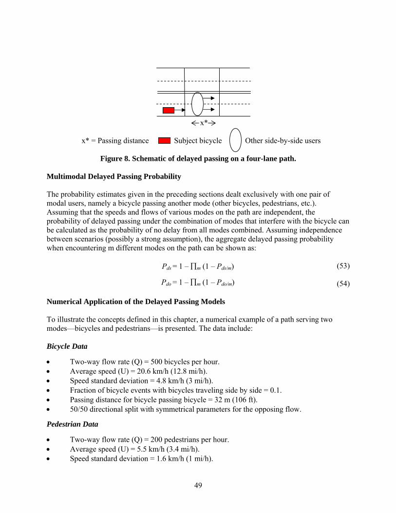
49

x* x* = Passing distance Subject bicycle Other side-by-side users

Figure 8. Schematic of delayed passing on a four-lane path. Multimodal Delayed Passing Probability The probability estimates given in the preceding sections dealt exclusively with one pair of modal users, namely a bicycle passing another mode (other bicycles, pedestrians, etc.). Assuming that the speeds and flows of various modes on the path are independent, the probability of delayed passing under the combination of modes that interfere with the bicycle can be calculated as the probability of no delay from all modes combined. Assuming independence between scenarios (possibly a strong assumption), the aggregate delayed passing probability when encountering m different modes on the path can be shown as: (53) (54)

Numerical Application of the Delayed Passing Models To illustrate the concepts defined in this chapter, a numerical example of a path serving two modes—bicycles and pedestrians—is presented. The data include: Bicycle Data

• Two-way flow rate (Q) = 500 bicycles per hour. • Average speed (U) = 20.6 km/h (12.8 mi/h). • Speed standard deviation = 4.8 km/h (3 mi/h). • Fraction of bicycle events with bicycles traveling side by side = 0.1. • Passing distance for bicycle passing bicycle = 32 m (106 ft). • 50/50 directional split with symmetrical parameters for the opposing flow. Pedestrian Data

• Two-way flow rate (Q) = 200 pedestrians per hour. • Average speed (U) = 5.5 km/h (3.4 mi/h). • Speed standard deviation = 1.6 km/h (1 mi/h).

Pds = 1 – ∏m (1 – Pds/m)

Pdo = 1 – ∏m (1 – Pdo/m)

50

• Fraction of pedestrians events with pedestrians traveling side by side = 0.35. • Passing distance for bicycle passing pedestrian = 18 m (60 ft). • 50/50 directional split with symmetrical parameters for the opposing flow. The example illustrates the difference in the probability of delayed passing for a two-, three-, or four-lane paths. Since flows and other parameters on the path are fully symmetrical, only the results for the subject direction are reported. Table 8 below summarizes all of the computations by mode and references the source equation for the calculation when applicable.

Table 8. Numerical illustration of path-width effect on delayed passing.

Two-Lane Path

Three-Lane Path

Four-Lane Path

Variables of Interest

Bikes Peds. Bikes Peds. Bikes Peds. Bicycle travel time (min) 4.7 4.7 4.7 4.7 4.7 4.7 Bicycle active passing events 1.83 21.6 1.83 21.6 1.83 21.6 Bicycle active passing rate per hour 23 276 23 276 23 276 Total desired passing rate per hour

299

299

299

Passing distance (Xm) in ft (assumed)

106

60

106

60

106

60

Density (Ksm) vehicles per mile = Q/U

19.5

29.4

19.5

29.4

19.5

29.4

Pvs/m (equation 37) 0.676 0.715 0.676 0.715 0.676 0.715Fbs/m (assumed) 0.1 0.35 0.1 0.35 0.10 0.35 Pbs/m (equation 49) 0 0 0.033 0.10 0.033 0.10

Pns/m (equations 39 and 50) 0.324 0.285 0.291 0.185 0.291 0.185Pds/m, % (equations 36, 47, and 49)

26.6

23.6

11.7

14.7

3.3

10.0

Pds, % (equation 53) 43.9 24.7 13.0 Number of delayed passings per hour

131

73.8

38.8

Mean time between delayed pass, s

27.5

48.8

93.0

1 ft = 0.3 m 1 vehicle per mile = 0.621 vehicles per kilometer

The first four rows in the table pertain to the calculation of desired passing events as described earlier in the chapter. The analysis yields a total of about 24 desired passing maneuvers (of slower bicycles and pedestrians) by a bicyclist traveling at the average speed while on the path. The effect that path widening would have on the quality of service is shown in table 8 as exemplified by the delayed passing probability and the average time between delayed passing events. By going from two to three lanes, the delayed passing probability is reduced by about

51

44 percent, and the time between delayed passing events increases from 27 to 49 s. Further widening to develop a four-lane path will result in an additional reduction of 48 percent in delayed passing and a comfortable time between delayed passing events of more than 1.5 min. The analysis shown can be extended for any combination of modes that may occur in the subject and opposing direction. Based on the field data gathered in this study, we applied the delayed passing method to 25 various combinations of modes in the subject and opposing directions. The combinations included a test bicycle passing each of the five modes that were at all common on the paths we studied (bicycles, child bicyclists, joggers, inline skaters, and pedestrians), while the opposing traffic consisted of each of those same five modes. Additional details on the application for multimodal users can be found in chapter 8 and the User’s Guide.

53

4. OPERATIONAL DATA COLLECTION INTRODUCTION One of the major objectives of this research was that the LOS methodology be calibrated and validated using data collected from the United States. The challenges facing the project team included a choice of methodology to allow the efficient collection of high-quality data on the operations of shared-use paths and the selection of study paths to provide a nationwide sample of representative paths. This chapter describes how the researchers met those challenges. Chapter 5 provides the results from the operational data collection effort. DATA COLLECTION METHOD The model for estimating the number of meetings and passings experienced by a test bicyclist developed in depth in chapter 3 uses the volume, average speed, and standard deviation around the average speed of each mode on the path as inputs. The data collection to calibrate and validate this model must therefore involve all of these variables. Of course, trail characteristics must also be recorded at each site. To ensure later flexibility, it was also desirable that scenes on paths of interest be recorded from different perspectives so that additional data could be obtained later by viewing videotapes if needed. The project team identified three possible methods of operational data collection, which included a one-camera method, a two-camera method, and a moving-bicycle method. The one-camera method involved a camera on a high perch that was able to record activity, including meetings and passings, on a long segment of path. The two-camera method involved two cameras set up several thousand feet apart along a path. From each camera, a sequence of users could be determined and, from those sequences, meetings and passings could be discerned. In the end, however, we concluded that the one-camera and two-camera methods would not provide adequate data, so we chose the moving-bicycle method (described below). Vantage points for the one-camera method would have been rare; tall buildings and hills with unobstructed views of qualifying shared-use paths are not common in the United States. The two-camera method would not have been able to identify the difference between actual passings and desired passings, because only path users would have known whether they wanted to pass and were unable to do so and why. For example, a bicyclist may not have been able to pass because of inadequate path width or congestion. We chose the moving-bicycle method as our primary operational data collection method because it overcomes the flaws in the other methods. It is not restricted to places where special camera vantage points are available, and it can determine desired passings. The method works by collecting data from the perspective of the bicyclist, and is analogous to the moving-vehicle method of collecting volumes and travel times on the highway (such as described in chapter 15 of the HCM(4)). In the moving-bicycle method, a member of the project team rides a bicycle along a path segment of interest at a predetermined constant speed. The team member attempts to maintain that speed as closely as possible, passing when encountering slower same-direction users when there is sufficient room to do so safely while maintaining that constant speed. The team member wore a video camera on his or her helmet that recorded the number of meetings,

54

the number of passings accomplished, and the number of passings delayed or not accomplished (i.e., reached the end of the segment before the opportunity to pass presented itself). At the same time, as the bicyclist was making his or her ride, a colleague was counting the number of users of each mode in each direction moving past the midway point of the segment. This provided the needed volume data. A potential bias with the moving-bicycle method is that data collector judgments determine the difference between a desired pass, a following maneuver with no desire to pass, and a completed pass. To prevent this bias from affecting the results, we equipped the bicycle with a mini-computer (a Specialized™ Speed Zone P.Brain) that displayed the bicycle speed to the nearest 0.16 km/h (0.1 mi/h). In addition, the team recorded the time needed to ride the segment from start to finish to verify that the desired speed was maintained. Moving-bicycle desired speeds were determined for each path based on the results of a prior study of the bicycle speed distribution on the path segment of interest. Typically, the data collection team conducted the prior study on the day before the moving-bicycle study was to commence. Therefore, the data collection process typically took 2 days per trail. On the first day, the team collected an adequate sample of speeds of the free-flowing bicycles (30 minimum) and of other path users using a stopwatch and a clearly marked distance. Then, the team calculated a mean and standard deviation for the bicycle speed sample. The moving-bicycle runs on the second day were typically made at three speed levels—high, medium, and low—that corresponded to the mean speed plus one standard deviation, the mean speed, and the mean speed minus one standard deviation from this prior sample. On the second day, the team collected the moving-bicycle data. We used a stationary camera on the side of the path at the midpoint, next to the volume data collector, to provide backup for the volume count, to provide additional speed observations, and to provide other data that may have proved necessary later. To avoid fatigue, the two data collectors traded bicycle duty and stationary volume counting duty occasionally. During the second day of data collection, the team set a goal to collect at least 20 runs at each of the three different speeds, or a total of 60 runs conducted at each path. Since we collected data for both directions along the trail, 60 runs actually provided 10 runs in each direction along the path at the three different speeds. Higher sample sizes would have been desirable, but were not usually possible, because user volumes on the paths of interest did not usually stay high for many hours of the day. We could only collect during daylight hours, and the bicycle riders became fatigued.

Equipment The main equipment for this data collection included a stationary camera/recorder, a bicycle, a mini video camera/recorder for the bicyclist’s helmet, and a bicycle speedometer. The bicyclist’s recorder was carried in a handlebar pouch, where the display was visible to the bicyclist, so that he or she could be sure that the system was recording. A microphone taped to the bicyclist’s shirt was incorporated into the mini-camera system to allow the bicyclist to record comments during a run The most helpful of these comments was whether a particular event was a delayed passing or not.

55

We used a hybrid bicycle, which is a combination of a mountain bicycle and a road bicycle, during our data collection. Hybrid bicycles have a smoother and wider tire than mountain bicycles in order to obtain the higher speeds and increased stability that we needed. The bicycle we used was also easy to disassemble and reassemble for travel by plane, because we attempted to use the same bicycle for all of the different data collection sites to ensure more consistency during the data collection process. In the end, mechanical problems with the bicycle meant that we used a rented bicycle during one of our data collection trips (to Saint Louis, MO). The mobile camera and recorder system we chose are generally used for surveillance operations. The mini-camera was approximately 50 millimeters (mm) (2 inches) long and 25 mm (1 inch) in diameter. The camera had 360 lines of resolution and a 3.6-mm-wide lens. The recorder was supposedly the world’s smallest VCR at the time we purchased it, with an LCD monitor that was about 190.5 mm (7.5 inches) by 114.3 mm (4.5 inches) by 88.9 mm (3.5 inches), weighing about 0.68 kilograms (kg) (1.5 pounds (lb)). The rechargeable camera battery lasted about 2 h. The research team soon developed a routine of changing all batteries and cassette tapes on all cameras and recorders every 2 h or 10 runs to ensure that we kept recording when desired. Total equipment costs for the cameras, bicycle, and accessories were about $3,000. SITE SELECTION The project budget allowed for operational data collection for up to 20 trails in 10 cities across the United States. This was likely to provide a large enough sample to calibrate and validate the procedure in a credible manner. The project team sought operational data collection sites that met a strict set of criteria to ensure project success. These criteria included: 1. Sites in most regions of the United States. 2. Two or more sites in a city in order to reduce travel costs and meet the goal of 20 path

segments in 10 cities. 3. Sites that were well known to trail planners and designers in order to build credibility in

the results. 4. Sites that had moderate to high traffic levels for at least some portions of some days. 5. Sites that had long segments with no intersections or turnouts (ensuring uninterrupted

flow). 6. Sites where the project team could unload equipment easily from a vehicle. 7. Sites that had a wide variety of geometric characteristics. 8. Sites with managers who were willing to cooperate. Based on the knowledge of the researchers and input from FHWA staff at the February 2001 briefing, the team assembled a preliminary list of possible data collection sites that may have met some or all of these criteria. The sites included: 1. Raleigh, NC: Shelly Lake Trail, Lake Johnson Trail, and Apex Lake Trail 2. Hilton Head Island, SC 3. Jekyll Island, GA 4. Pinellas County, FL: Pinellas Trail 5. Gainesville, FL: Gainesville-Hawthorne Trail

56

6. Tallahassee, FL: St. Mark’s Trail 7. Winter Garden and Apopka, FL: West Orange Trail 8. Orlando, FL: Cady Way Trail 9. Boston and Cambridge, MA: Charles River Trail 10. Arlington, Bedford, and Lexington, MA: Minuteman Bikeway 11. White Plains, NY: North County Trailway and South County Trailway 12. Manhattan, NY: Hudson River Trail from Battery Park to 125th Street 13. Brooklyn, NY: Shore Parkway and Ocean Parkway 14. Philadelphia, PA: Schuylkill River Trail 15. Washington, DC: Capital Crescent Trail and Washington and Old Dominion Trail 16. Virginia Beach, VA 17. Chicago, IL: Lakefront Path 18. Mackinac Island, MI: M-185 19. Madison, WI 20. St. Louis, MO: Forest Park Bike Path and Grant’s Trail 21. Columbia, MO 22. Phoenix, AZ 23. Tucson, AZ 24. Denver, CO: Platte River Greenway and Cherry Creek Path 25. Houston, TX: Harrisburg Rail Trail, West White Oak Bayou Trail, West Brays Bayou

Trail System, and Buffalo Bayou Trail 26. Dallas, TX 27. Davis, CA 28. Huntington Beach, CA: Bolsa Chica-Huntington Beach 29. Los Angeles, CA: South Bay Trail 30. Santa Ana, CA: Santa Ana River Trail 31. Santa Monica, CA: Ocean Front Walk 32. San Diego, CA: Ocean Front Walk 33. San Francisco and Oakland, CA: San Francisco Bay Trail 34. Portland, OR 35. Seattle, WA: Burke-Gilman Trail 36. Boulder, CO 37. Portland, ME The project team developed a questionnaire for the owners or managers of the paths listed above to determine the suitability of a particular path for data collection. The questionnaire asked: 1. Is the trail paved? 2. What is the length of the shortest uninterrupted segment? 3. Which user modes use this trail? 4. What is the predominant user mode? 5. Are the trail users mainly recreational users or commuters? 6. Is the trail divided by a median, berm, or pavement striping? 7. What is the width of the trail? 8. Would you consider the trail volumes to be high, medium, or low? 9. What is the peak month of the year?

57

10. What is the peak day of the week for the trail? 11. What is the peak time of the day for the trail? 12. How would you describe the trail grades (level, rolling, or mountainous)? 13. Would we be able to park a vehicle near the trail? 14. Do we need permission to conduct our study along your trail? The project team sent the questionnaire to the owners or managers of the 37 trails via regular mail and e-mail and received 26 responses. From the responses, the researchers identified a list of 10 cities and an alternate city that provided the best possible opportunities to satisfy the criteria. The list included cities in all regions of the United States and cities with many of the best-known trails in the United States. The final list of sites approved by FHWA was: 1. Seattle, WA 2. San Francisco, CA 3. Boston, MA 4. Chicago, IL 5. St. Petersburg, FL 6. St. Louis, MO 7. Raleigh, NC 8. Dallas, TX 9. Washington, DC 10. Denver, CO 11. Los Angeles, CA (alternate) In the end, we used our alternate city, Los Angeles, and did not collect data in Denver because of travel and weather difficulties. In the course of this study, the team collected data from 15 trails and 10 cities scattered across the United States. Some cities only had one usable trail. The data collection sites were: 1. Lake Johnson Trail in Raleigh, NC 2. Pinellas Trail and Honeymoon Island Trail near St. Petersburg, FL 3. White Creek Trail and White Rock Lake Trail in Dallas, TX 4. Mill Valley-Sausalito Pathway near San Francisco, CA 5. South Bay Trail in Santa Monica, CA 6. Sammamish River Trail near Seattle, WA 7. Forest Park Trail and Grant’s Farm Trail in St. Louis, MO 8. Lakefront Trail in Chicago, IL 9. Dr. Paul Dudley Bike Path and Minuteman Bikeway in and near Boston, MA 10. Capital Crescent Trail and Washington and Old Dominion Trail near the District of Columbia The most restrictive criteria in terms of locating usable trail segments were the segment length and the need for moderate to high volumes of traffic. Trails with moderate to high volumes of traffic tend to be in areas with many intersections and trail connections; however, we wanted segments at least 0.8 km (0.5 mi) long between intersections to gather unbiased data using the moving-bicycle method. In the end, we compromised on segment length in a couple of places (a

58

0.40-km (0.25-mi) segment for the South Bay Trail and a 0.64-km (0.4-mi) segment for the Forest Park Trail). We settled for segments in other places that did not have very high volumes, as shown in chapter 5. Tables 9 and 10 provides some details on the chosen study trails. The study trails were located in urban and suburban areas. The study trail environments included parks, lakes, beaches, highways, and downtown areas. There was a nice range of trail widths from 2.44 m to 6.1 m (8 to 20 ft). The study trails were sometimes marked with centerlines, and sometimes there were other adjacent treadways that accommodated some users. Few trails had significant horizontal or vertical curvature. Most trails had good sight distances, as judged qualitatively by the research team after riding them numerous times on a bicycle.

Table 9. Characteristics of operational study sites.

Location Path name Community

context Trail type Study location Area

landscape Width

(ft) Centerline

Raleigh, NC

Lake Johnson Trail Suburban Park loop

0.25 mile point to the 0.75 mile point

Wooded park, lake 8–8.5 None

Redmond, WA

Sammamish River Trail Suburban

Linear riverside greenway

In Sixty Acre Park, about 0.5 mi from NE 116th St.

Grass, ballfields 10 None

Marin County, CA

Mill Valley-Sausalito Pathway Suburban Rail-trail

At Bothin Marsh, north of the U.S. 101 bridge

Marsh, highway, bay

9.5–10.5 None

Dallas, TX White Rock Lake Trail Urban Park loop

Just south of the E. Lawther/Emerald Is. park access, near Winfrey Point

Grass, lake, park road 14 Solid

Chicago, IL Lakefront Trail Urban

Lakefront beach trail

Near trail intersection with North Avenue

Grass and beach 20 Solid

Santa Monica, CA

South Bay Trail Suburban

Oceanfront beach trail

About a mile north of the Santa Monica Pier Beach 14 Dashed

St. Louis, MO

Forest Park Trail Urban Park loop

On the north edge of the park, along Lindell Blvd., between mile 5.25 and 5.75

Grass and street 10 Solid

Dunedin, FL

Honeymoon Is. Trail (Dunedin Causeway) Suburban

Hwy. sidepath/ greenway

West of the drawbridge

Beach, roadway 12 None

Arlington, MA

Minuteman Bikeway Suburban Rail-trail

Mile marker 7.5 near the bike shop Wooded 12 Dashed

Boston, MA

Dr. Paul Dudley Bike Path Urban

Linear riverside greenway

South of the River, just east of the Harvard Br.

River, highway 8 Dashed

59

Table 9. Characteristics of operational study sites (continued).

Location Path name Community

context Trail type Study location Area

landscape Width

(ft) Centerline

Vienna, VA W&OD Trail Suburban Rail-trail

Near downtown Vienna

Grass and trees 10 Solid

Washington, DC

Capital Crescent Trail Urban Rail-trail

Between K St. and Fletcher's Boathouse Wooded 10 Dashed

St. Louis Co., MO

Grant's Trail Suburban Rail-trail

Near I-55 and Union Road

Grass and trees 12 Solid

Dunedin, FL

Pinellas Trail Suburban Rail-trail

North of Curlew Road

Golf course and hwy. 15 Solid

Dallas, TX White Creek Trail Suburban

Linear streamside greenway

North of the Fair Oaks Tennis Center, on both sides of the overpass

Grass, stream 8 None

1 ft = 0.305 m 1 mi = 1.61 km

Table 10. Additional characteristics of operational study sites.

Location Path name Surface Shoulder Other

treadways Clear

zone (ft) Sight

distance Horizontal curvature

Vertical curvature

Raleigh, NC

Lake Johnson Trail

Asphalt (in poor condition) No None 1 to 4 Poor Medium Low

Redmond, WA

Sammamish River Trail Asphalt No Horse trail 6 to 10 Good Low Low

Marin County, CA

Mill Valley-Sausalito Pathway Asphalt

Yes, 5-7 ft gravel None 5 to 7 Unlimited Low No

Dallas, TX White Rock Lake Trail

12 ft of asphalt with 1 ft concrete edges No

Some bicyclists use park road 10 to 20 Unlimited Low No

Chicago, IL Lakefront Trail Concrete No None Unlimited Good None No

Santa Monica, CA

South Bay Trail Concrete No None Unlimited Unlimited Low No

St. Louis, MO

Forest Park Trail Asphalt

Yes, 4 ft dirt on one side

Joggers use 4 ft dirt shoulder 4 Good None No

Dunedin, FL

Honeymoon Is. Trail (Dunedin Causeway) Asphalt No None

0 on one side, 4 on the other Unlimited Low No

60

Table 10. Additional characteristics of operational study sites (continued).

Location Path name Surface Shoulder Other

treadways Clear

zone (ft) Sight

distance Horizontal curvature

Vertical curvature

Arlington, MA

Minuteman Bikeway Asphalt No None 2 to 4 Fair None No

Boston, MA

Dr. Paul Dudley Bike Path Asphalt No

Separate ped. paths None Poor Medium No

Vienna, VA W&OD Trail Asphalt No None Unlimited Excellent Low No

Washington, DC

Capital Crescent Trail Asphalt No

Peds. Use adjacent towpath 2 to 4 Unlimited Low No

St. Louis Co., MO

Grant's Trail Asphalt No None 2 to 4 Good Low No

Dunedin, FL

Pinellas Trail Asphalt No

Some ped. paths 6 to 10 Unlimited None No

Dallas, TX White Creek Trail Asphalt No None 30 to 75 Unlimited None No

1 ft = 0.305 m 1 mi = 1.61 km

DATA COLLECTION EXECUTION Data collection occurred from July 2001 to March 2002. Peak hours and peak times were identified for each trail location. The peak days were generally Saturdays and Sundays. Peak hours varied by location. There often appeared to be two peaks during the weekend days on most trails; one volume peak in the morning and a second volume peak in the afternoon. Trail users who appeared to be using the trail for fitness purposes appeared most often during the morning hours. Recreational and casual users, consisting of tourists and families, appeared more often during the afternoons. At data collection sites where there were commuters, the commuter peak hours were generally the weekday mornings. The data collection process generally lasted from early morning until dusk; consequently, a great variation in volume was typically collected at each site.

61

The data collection team attempted to collect 60 trials at each trail. Because of inclement weather and mechanical failures, it was not possible to obtain 60 trials at each trail location. In total, 771 runs were successfully completed. Table 11 shows the sample size by trail. Because it was such a high-quality site and there were no other candidate sites in the city, the team collected extra data at the Lakefront Trail in Chicago. The most disappointing data collection trip was to Washington, DC, during October 2001, when bad weather prevented all but a handful of runs at what should have been excellent data collection sites.

Table 11. Number of successful data collection runs by trail. Trail Successful Runs

Lake Johnson 58 Sammamish River 58 Mill Valley-Sausalito 60 White Rock Lake 60 White Creek 60 Lakefront 90 South Bay 60 Grant’s 30 Forest Park 57 Honeymoon Island 48 Pinellas 57 Minuteman 60 Dr. Paul Dudley 60 Capital Crescent 9 Washington & Old Dominion 4 Total 771

63

5. OPERATIONAL DATA ANALYSIS

INTRODUCTION After the operational data collection process described in chapter 4, the research team analyzed the data from both the static and mobile vantage points. The analysis had two main objectives. First, the team wanted to develop a series of average and default values for key parameters that it could use as it developed the LOS estimation procedure. The speed samples collected were obviously an important part of this. Other important values to be determined from the data included the PHF and the percentage of each user group that traveled in groups of two or more mode users. The second objective of the analysis was to compare the measured number of meetings and passings against the number of meetings and passings predicted from the theory developed in chapter 3. This comparison would validate the theory applicable to typical U.S. shared-path conditions. This chapter describes how the project team met both of these main objectives. AVERAGE AND DEFAULT VALUES Speed As was noted in chapter 4, the project team recorded speed samples at each trail for each representative user group. The measurement was manual, with a stopwatch, and the team’s goal was a sample of at least 30 free-flowing bicyclists and as many other path users as appeared during the recording of the bicyclists’ speeds. In the cases of the Lakefront and Sammamish River Trails, since the team collected data at two different places along the trail, we collected more than 30 bicycle speeds for the sample. The team did not collect usable speed data on the Washington, DC, area trails because of poor weather conditions. Since most bicyclists and other path users traveled the sample paths as individuals instead of in groups (as will be seen below), these free-flowing average speeds are probably quite similar to the overall average speeds. Table 14 shows a summary of the speed data we collected. The table shows the sample size, average speed, and standard deviation around that average for each mode at each trail. The table also shows, for each mode, the average of the 13 trail average speeds and the average and standard deviation of the total set of observations. The average speed for the 443 adult bicyclists observed was 20.62 km/h (12.81 mi/h), with a standard deviation of 5.49 km/h (3.41 mi/h). Average bicycle speeds on the paths ranged from almost 24.15 km/h (15 mi/h) on the Pinellas Trail in Florida—a wide, straight, and flat path used by many fitness riders—to more than 16.1 km/h (10 mi/h) on the Lake Johnson Trail in Raleigh, NC—a narrow, curvy, bumpy path. The 20.60 km/h (12.8 mi/h) average is just slightly higher than values reported in the literature—perhaps because most segments studied had at least 0.80 km (0.5 mi) uninterrupted by intersections or turnouts, and because we broke out child bicyclists as a separate mode. The average speed for the 275 pedestrians observed was 5.42 km/h (3.37 mi/h); pedestrian speeds were more uniform than bicycle speeds across trails (discounting the sites with only a handful of observations). Based on samples of more than 200 users for each mode, the average inline skater speed was 16.30 km/h (10.13 mi/h), while the average jogger speed was 10.40 km/h (6.46 mi/h). The average child bicycle speed was 12.64 km/h (7.85 mi/h), but this was based on a sample of

64

only 29 users. Overall, the speed data in table 12 are sufficient for use in an LOS procedure in cases where the trail designer or manager does not have a sample for the specific trail.

Table 12. Speeds by mode and trail (all speeds in mi/h). Mode: Bicycle Pedestrian Inline skater Runner Child Bicyclist

Trail N Mean Std.Dev. N Mean

Std.Dev. N Mean

Std.Dev. N Mean

Std.Dev. N Mean

Std.Dev.

PD 29 12.74 2.60 5 4.06 0.50 24 9.37 1.76 9 7.68 1.23 0 M 29 14.32 3.40 8 3.59 0.35 21 11.22 2.72 5 6.91 1.24 1 9.98 P 25 14.96 3.98 2 4.79 0.28 6 13.68 5.48 3 7.18 1.38 0

HI 30 11.22 3.57 29 3.49 0.52 8 8.61 2.39 15 6.43 0.65 0 FP 26 13.78 3.18 16 3.64 0.63 15 11.15 3.14 8 7.07 1.09 0 G 30 12.30 3.28 16 3.55 0.48 15 10.11 1.41 8 6.59 1.17 0 SB 30 10.66 3.22 30 3.17 0.35 30 9.71 2.06 29 5.83 0.85 2 7.19 0.87 LF 60 12.60 3.15 46 3.16 0.57 53 10.94 2.68 46 6.99 0.97 0 WC 30 11.87 2.29 31 3.07 0.49 31 8.20 2.11 31 6.33 1.18 10 7.56 1.80 WR 31 14.27 3.01 25 3.02 0.43 6 8.86 3.62 33 5.44 0.89 6 9.46 0.84 MV 30 14.58 3.08 30 3.52 0.54 0 30 6.63 1.23 2 4.88 0.83 SR 63 13.23 3.35 7 3.09 0.48 9 11.41 2.17 13 5.80 1.44 5 8.16 1.84 LJ 30 10.40 2.80 30 3.83 0.60 1 7.25 30 6.99 1.09 3 6.83 2.78

All* 13 12.84 1.51 13 3.54 0.49 12 10.04 1.75 13 6.61 0.63 7 7.72 1.71 All** 443 12.82 3.41 275 3.37 0.59 219 10.13 2.75 260 6.46 1.20 29 7.85 1.95

* Over trails ** Over samples Key to trail names: PD = Paul Dudley, M = Minuteman, P = Pinellas, HI = Honeymoon Is., FP = Forest Park, G = Grant’s, SB = South Bay, LF = Lakefront, WC = White Creek, WR = White Rock, MV = Mill Valley, SR = Sammamish River, LGJ = Lake Johnson. 1 mi/h = 1.61 km/h

Volume and Mode Split Some trail designers and managers will have detailed counts or forecasts of the volumes of users by mode expected on their paths. However, most will not have such detailed data and will need to rely on default values for those inputs. Our data set, based on up to 8 h of observation at relatively busy (if not peak) times on each of 15 well-known paths across the United States, may serve well in providing those default values. Table 13 shows a summary of our volume and mode-split data by trail. This table includes all 15 trails, from the data recorded manually at the midpoint of the segment of interest; the volumes are from both directions of travel on the path. From table 13, we note that adult bicyclists made up the majority of the trail users overall and on most trails, with 56 percent of the user share overall. This ranged from a high of 81 percent on the Pinellas Trail to a low of 14 percent on the Lake Johnson Trail; these are the same trails that were the extremes for bicycle speeds as well. Pedestrians made up 18 percent of the trail users overall, with a range of 63 percent on the Lake Johnson Trail to 3 percent on the Sammamish River Trail. Inline skaters were 10 percent of the users observed, joggers were 13 percent of the users observed, and child bicyclists were 3 percent of the users observed. Some trails did not have any skaters, and others did not have any child bicyclists. There was a wide range of volumes exhibited across trails, ranging from an average of more than 2,300 users per hour on the four-lane Chicago Lakefront Trail during a

65

sunny summer weekend to just 44 users per hour on the Washington and Old Dominion Trail in cold, windy, and rainy conditions. The average of the average volumes per trail was 426 users per hour, although there was a large standard deviation around that average.

Table 13. Volumes and mode splits by trail. Bicycles Pedestrians Skaters Runners Child Bikes

Trail Per hour

% of total

Per hour

% of total

Per hour

% of total

Per hour

% of total

Per hour

% of total

Total per

hour PD 317 72 36 8 64 15 17 4 5 1 438 M 229 52 28 6 80 18 69 16 36 8 442 P 98 81 6 5 14 12 3 2 0 0 120 HI 25 23 60 54 9 8 14 13 2 2 110 FP 99 33 73 24 42 14 83 28 3 1 299 G 73 59 20 16 13 10 5 4 13 10 123 SB 248 40 107 17 154 25 77 12 30 5 616 LF 1131 49 474 20 286 12 410 18 15 1 2317 WC 140 65 21 10 31 14 14 7 10 4 217 WR 180 72 34 14 9 3 20 8 9 3 252 MV 402 63 50 8 0 0 178 28 11 2 641 SR 330 79 14 3 25 6 14 3 35 8 418 LJ 29 14 130 63 0 0 45 22 2 1 205 CC 89 59 27 18 5 4 30 20 0 0 151 WO 32 74 2 5 2 5 7 16 0 0 44 Ave. 228 56 72 18 49 10 66 13 11 3 426 Std. dev. 277 20 117 18 77 7 106 9 13 3 554

Key to trail names: PD = Paul Dudley, M = Minuteman, P = Pinellas, HI = Honeymoon Is., FP = Forest Park, G = Grant’s, SB = South Bay, LF = Lakefront, WC = White Creek, WR = White Rock, MV = Mill Valley, SR = Sammamish River, LJ = Lake Johnson, CC = Capital Crescent , WO = W&OD 1 mi/h = 1.61 km/h

The research team was concerned about the wide variations in volume and mode split observed at the sample trails because users may lack confidence in using these results as default values in their analyses when local data are unavailable. In particular, the Lake Johnson Trail had a very different mode split than the other trails, the Washington and Old Dominion had much lower volumes than the other trails, and the Lakefront Trail had much higher volumes than the other trails. However, recomputing the average mode splits and volumes without these trails made very little difference in the averages, except for the case of the Lakefront Trail. Dropping the Lakefront Trail meant that the average volume declined to 291 users per hour. In the end, it appears that mode split and volume are simply parameters that will vary widely from trail to trail; consequently, trail designers and managers are going to have to consider that variation in their analyses. The User’s Guide provides some suggestions as to how this can be done in some typical analyses.

66

Peak-Hour Factor The PHF is an important consideration used in capacity and LOS calculations to adjust for peaking of traffic within the hour of interest. Since a 15-minute (min) timeframe is used for determining an LOS in the HCM,(4) the PHF for this procedure will also be based on 15 min. The equation for determining the PHF is:(4)

PHF = v / (4 * V) (55) where v is the hourly volume and V is the volume of users in the peak 15-min time period within the hour. Values of PHF for shared-use paths are not readily available in practice or in the literature; therefore, using our data to find an average or default PHF should be helpful. The volume data collected manually and summarized in table 13 were not from continuous counts; instead, the data collector only counted while the bicyclist with the helmet camera was moving. This made computation of a PHF from those data very difficult. To compute an average PHF, we turned to the images recorded by the static camera. We selected tapes in which good weather and good equipment performance allowed continuous 1-h counts. Table 14 shows data that we collected from the static camera for this purpose.

67

Table 14. PHF data. Trail Time Users per

Hour Peak-Hour

Factor 10:30 a.m. 192 0.889 11:35 a.m. 203 0.875

White Rock

12:35 p.m. 173 0.901 12:50 p.m. 311 0.770 1:50 p.m. 361 0.771 3:38 p.m. 320 0.920

Sammamish River

5:40 p.m. 187 0.698 9:50 a.m. 352 0.815 12:30 p.m. 402 0.831

Minuteman

2:30 p.m. 401 0.928 2:30 p.m. 319 0.798 4:30 p.m. 333 0.876

Paul Dudley

7:00 p.m. 190 0.819 10:30 a.m. 163 0.728 12:30 p.m. 166 0.988

Lake Johnson

3:00 p.m. 229 0.806 11:00 a.m. 1766 0.901 1:00 p.m. 2056 0.948

Lakefront

6:00 p.m. 1132 0.901 10:00 a.m. 112 0.885 12:00 p.m. 310 0.765

Mill Valley-Sausalito

2:00 p.m. 197 0.723 11:00 a.m. 296 0.903 South Bay 1:00 p.m. 321 0.912

Average 437 0.848 Standard Deviation 496 0.078

Table 14 shows that the average hourly volume for the time periods sampled was almost equal to the average hourly volume from the full data set in table 13. Based on those time periods, an average PHF was about 0.85. The standard deviation of about 0.08 around that average PHF shows that there was some variation from trail to trail and hour to hour. One trend worth noting was that, as expected, PHF tended to rise as the hourly volume rose. Figure 9 shows the trend, which was heavily influenced by the high-volume Chicago observations.

68

Figure 9. PHF as a function of hourly volume. Users Occupying Two Lanes The researchers needed the proportion of users moving along the path while occupying two lanes as an input to the delayed passing procedure developed in chapter 3. Usually, a group of two users moving together would occupy two lanes. However, there were many cases where two users moving together occupied less than two lanes because they moved in single file, one walked or rode off the path, or they walked or rode very close to each other. There were also cases when a single path user occupied two lanes. This was typically an inline skater swinging his or her arms and legs widely, although there were also cases when a weaving, wobbling bicyclist used two lanes. Thus, to collect data on this proportion, we had to carefully examine the movements of each user or group of users. The static camera did not provide a perspective that showed how much of the path a user or group of users was occupying; therefore, we had to use the video recorded by the mobile (helmet) camera. We reviewed 21 h of runs on seven paths (all the times and trails listed in table 14, except the Chicago Lakefront, where these data were too difficult to collect). In that sample, we observed the following proportions:

0.6

0.7

0.8

0.9

1.0

0 500 1000 1500 2000 2500

User volume per hour

Peak

-Hou

r Fac

tor

69

• Bicyclist groups occupied two lanes in 140 of the 2,691 cases observed (5 percent). • Pedestrian groups occupied two lanes in 252 of the 698 cases observed (36 percent). • Jogger groups occupied two lanes in 66 of the 536 cases observed (12 percent). • Skater groups occupied two lanes in 39 of the 493 cases observed (8 percent). • Child bicycle groups occupied two lanes in 1 of the 202 cases observed (0.5 percent).

We note that a “group” in this context consisted of one or more path users who seemed to be moving along the path together. Distance Needed to Pass Another factor needed as an input to the delayed passing procedure developed in chapter 3 is the distance needed to pass. To collect these data, we needed high-quality images with many passing maneuvers on paths that were of moderate width. In the end, we reviewed 50 runs in which high-quality video with passing maneuvers was available on five paths (Grant’s, Forest Park, Minuteman, Sammamish River, and Honeymoon Island). These paths are 3 to 3.6 m (10 to 12 ft) wide. Table 15 shows the data for the case of the experiment bicycle passing a pedestrian. The overall average distance is 29.89 m (98 ft), and the average did not change much when the experiment bicycle was traveling from 17.71 to 22.54 km/h (11 to 14 mi/h) (near the overall average bicycle speed). We did not have nearly as large sample sizes for the bicycle passing other modes; however, the samples we recorded were:

• 49.7-m (163-ft) average distance to pass a bicycle, based on four observations. • 48.1-m (158-ft) average distance to pass an inline skater, based on four observations. • 31.7-m (104-ft) average distance to pass a jogger, based on seven observations.

We did not examine a case where the experiment bicycle passed a child bicyclist during the 50 runs examined. The field data for the distance needed to pass were difficult to collect and may not be representative of actual passings for several reasons. First, our data collectors were trying to maintain a constant speed, even while passing, while normal bicyclists would probably speed up during the pass. Second, our data collectors were probably much more conservative in making a passing than were the regular bicyclists, who would probably use longer gaps before and after making the pass. Third, since our runs were only 0.80 km (0.5 mi) long (or shorter in a few cases), we were only passing the slowest bicyclists.

70

Table 15. Distance needed for a bicycle to pass a pedestrian. Passing a ped. group occupying one lane Passing a ped. group occupying two lanes Time, sec Speed, mi/h Distance, ft Time, sec Speed, mi/h Distance, ft

5.81 7.8 66 9.16 7.8 105 7.22 8.3 88 9.35 7.8 107 5.53 8.3 67 9.75 8.0 114 4.28 8.4 53 10.41 8.5 130 4.66 8.4 57 5.53 8.6 70 8.06 8.5 100 5.00 10.0 73 6.24 9.3 85 7.69 10.1 114 9.15 9.4 126 6.65 10.3 100 3.28 9.4 45 5.31 11.8 92 4.07 9.4 56 8.00 11.8 138 5.31 10.1 79 6.94 12.2 124 5.04 10.3 76 5.91 13.3 115 7.62 10.7 120 4.94 13.4 97 7.94 10.9 127 5.10 14.6 109 6.75 11.3 112 5.97 14.8 130 5.59 11.3 93 6.93 14.8 150 5.59 12.1 99 4.35 14.8 94 4.75 12.2 85 5.19 15.3 116 4.56 12.2 82 4.97 15.3 112 5.50 12.3 99 – – – 5.56 12.6 103 – – – 4.50 13.4 88 – – – 3.62 14.5 77 – – – 4.09 14.8 89 – – – 4.78 16.4 115 – – – 4.72 17.3 120 – – –

Overall average 89 Overall average 110 Ave. for speeds 11–14 mi/h 95 Ave. for speeds 11–14 mi/h 113

1 ft = 0.305 m 1 mi/h = 1.61 km/h To supplement the small samples of somewhat questionable field data on the distance needed to pass, the project team developed a model. The basis of the model is the simple idea that the distance needed to pass is equal to the gap before the pass, plus the gap after the pass, plus the distance traveled during the passing by the user being passed. The terms of this model are in equation 56: (56) where DP is the distance needed to complete a passing (in ft), BG is the gap between the passer and the user to be passed at the beginning of the passing (in ft), EG is the gap between the passer and the user that was passed at the end of the passing (in ft), PS is the speed of the passer

DP = (BG + EG) * PS/(PS – SS)

71

(in ft/s), and SS is the speed of the user being passed (in ft/s). Since the mean speeds of the modes, other than bicycles given in table 14 above, are so much less than the mean bicycle speed, it is a safe assumption to use the mean speeds of those other modes as the appropriate values for SS in equation 47. However, the mean speeds of bicycles being passed would be considerably less than the overall bicycle mean speed if the passing bicycle is assumed to travel at the mean speed. To estimate SS for bicycles, then, the researchers developed a simulation of operations on a path that randomly assigned speeds to bicyclists along the path, based on the assumption that bicycle speeds are normally distributed (see later in the chapter); the researchers then tracked the speeds of bicycles that were passed by a test bicycle traveling at the overall mean speed. Based on a test bicycle and an overall bicycle mean speed of 20.6 km/h (12.8 mi/h), a standard deviation of 5.49 km/h (3.41 mi/h) around that mean speed, and a volume of 115 bicycles per hour in one direction (the average volume across all paths from table 15), the SS for passed bicycles was about 12.88 km/h (8 mi/h) or 3.66 m/s (12 ft/s). Using PS = 20.61 km/h (12.8 mi/h) or 5.73 m/s (18.8 ft/s), SS as described above, and BG = EG = 6.1 m (20 ft) (which we believe to be reasonable for many passing situations), the researchers produced the values in the column labeled “Estimated” in table 18. As one can see, the estimated values in table 18 are about two-thirds of the field average values for bicycles, skaters, and joggers, and about one-half of the field average value for pedestrians.

Table 16. Summary of distance needed to pass values. Distance needed for bicycles to pass, ft

Mode Field average Estimated Assumed Bicycles 163 110 100

Pedestrians 98 49 60 Skaters 158 87 100 Runners 104 61 70

Child Bikes None 69 70 1 ft = 0.305 m

The column labeled “Assumed” in table 16 shows the values of distance to pass that the team used in the delayed passing spreadsheet that became a part of the LOS procedure (see chapter 8). We assumed a lower value for passing bicycles because we believe that BG and EG are typically lower than 6.1 m (20 ft) when the passing user is traveling nearly the same speed as the user being passed since path users try to minimize the time that they are in the middle or opposing lane. For pedestrians, skaters, and joggers, we assumed values between the field average and estimated values, but closer to the estimated values, because the field data were based on very conservative bicycling practices. Finally, with no relevant field data on hand, we assumed that the distance required to pass a child bicyclist was nearly the same as the estimated value. VALIDATING THEORY Besides providing the important average and default values described above, the other major purpose of the operational data collection was to validate the theory developed in chapter 3 on predicting the number of meetings and passings along a path. In this section, we first show that the key assumption in chapter 3—that user speeds are normally distributed—was a sound one.

72

We then compare the theoretical predictions of meetings and passings to the field data for a variety of paths and show that the theory generally matched the field data reasonably well. Speeds Normally Distributed The assumption that user speeds are normally distributed was key in chapter 3, and the field data we collected generally prove that the assumption was sound. Figures 10 through 14 show the distributions of the speeds observed during our data collection (the same data set as described in table 12 above) by mode. All of the distributions look normal, with the exception of a couple of points. More convincing evidence is provided in table 16 for all modes except for child bicyclists, for whom the sample size was too small. Table 16 shows the results of chi-square tests comparing the distribution of speeds collected in the field to a theoretical normal distribution of speeds with a mean and standard deviation as reported in table 12. The chi-square test is well known and commonly used for this purpose (e.g., see May’s classic text, Traffic Flow Fundamentals).(60) Table 17 shows that the field and theoretical normal distributions were not significantly different at the 0.05 level for the cases of the bicycle, pedestrian, and skater modes. Joggers were the only mode for which there was a significant difference. Table 17 shows that the difference was only because of an overabundance of relatively slow (8.05 km/h (5 mi/h)) joggers. Overall, the field data provide convincing evidence that user speeds on the shared-use paths that we studied were normally distributed.

73

1 mi/h – 1.61 km/h

Figure 10. Distribution of bicycle speed data.

1 mi/h = 1.61 km/h

Figure 11. Distribution of pedestrian speed data.

0 10 20 30 40 50 60 70 80 90

0 1 2 3 4 5 Speed, mi/h

Num

ber o

f obs

erva

tions

0

10

20

30

40

50

60

0 5 10 15 20 25

Speed, mi/h

Num

ber o

f obs

erva

tions

74

1 mi/h = 1.61 km/h

Figure 12. Distribution of skater speed data.

1 mi/h = 1.61 km/h

Figure 13. Distribution of jogger speed data.

0

5

10

15

20

25

30

35

40

0 5 10 15 20 25

Speed, mi/h

Num

ber o

f obs

erva

tions

010

20 30 40

50 60 70

80 90

0 5 10 15

Speed, mi/h

Num

ber o

f obs

erva

tions

75

1 mi/h = 1.61 km/h

Figure 14. Distribution of child bicyclist speed data.

0123456789

10

0 5 10 15

Speed, mi/h

Num

ber o

f obs

erva

tions

76

Table 17. Chi-square test results comparing field and

normal distributions for speed data. Frequency

Mode

Speed, mi/h Counted Theoretical

Chi-square value6 and lower 5 14 6.0

7 16 12 1.3 8 23 20 0.6 9 34 28 1.5 10 39 36 0.2 11 53 46 1.1 12 44 50 0.6 13 50 53 0.1 14 47 48 0.0 15 44 42 0.1 16 27 34 1.5 17 21 24 0.4 18 15 17 0.1 19 9 10 0.1 20 5 6 0.1 21 7 3 5.5

22 and higher 4 2 1.2 Sum 20.4

Critical chi-square value at 0.05 level 23.7

Bicycle

Significant difference? No 2 8 8 0.0

2.5 27 33 0.9 3 85 75 1.3

3.5 83 88 0.2 4 54 53 0.0

4.5 14 16 0.3 5 4 3 0.7

Sum 3.4 Critical chi-square value at 0.05 level 9.5

Pedestrian

Significant difference? No 1 mi/h = 1.61 km/h

77

Table 17. Chi-square test results comparing field and normal distributions for speed data (continued).

Frequency Mode

Speed, mi/h Counted Theoretical

Chi-square value

5 and lower 6 10 1.8 6 10 10 0.0 7 18 17 0.1 8 24 24 0.0 9 37 29 2.4 10 38 32 1.1 11 24 30 1.0 12 21 25 0.5 13 15 18 0.7 14 13 11 0.2 15 4 6 1.0 16 4 3 0.2

17 and higher 4 2 1.6 Sum 10.6

Critical chi-square value at 0.05 level 18.3

Skater

Significant difference? No 4 & lower 6 10 1.9

5 53 36 7.8 6 81 76 0.4 7 69 80 1.4 8 40 44 0.4 9 8 13 1.8

10 and higher 4 2 1.9 Sum 15.7

Critical chi-square value at 0.05 level 9.5

Runner

Significant difference? No 1 mi/h = 1.61 km/h

Comparing Predicted Meetings and Passings to Field Data Chapter 3 described the development of a theory on how to estimate the number of meetings and passings by a test bicyclist on a path, given the traffic volumes and speeds of the various modes on the path. To gather the field data against which those estimates will be compared, a team member viewed the videotapes recorded from the helmet camera and documented the number of meetings and active passing events that occurred during each trial. The researchers did not document passive passing events since very few of them were seen on the mobile video. Table 18 shows a summary of the meetings and passings (completed and desired) data in terms of average values per trail. Table 18 does not report data from the two Washington, DC, area trails since those sample sizes were so small and the data were so unstable that they were not helpful. Obviously, there was good variation in meetings and passings per mile. The test bicycle

78

on the Lakefront Trail in Chicago met an average of 120 trail users per mile, while the test bicycle only met an average of nine trail users per mile on the Pinellas and Grant’s trails. The test bicycle on the Lakefront Trail passed an average of 21 trail users per mile, while passing an average of 2 trail users per mile on the Pinellas and Grant’s Trails.

Table 18. Average meetings and passings on each trail.

Trail Average user

volume per hour Average meetings

per mile Average passings

per mile Paul Dudley 438 31 3 Minuteman 442 27 5 Pinellas 120 9 2 Honeymoon Is. 110 13 5 Forest Park 299 22 6 Grant's 123 9 2 South Bay 616 61 12 Lakefront 2317 120 21 White Creek 217 16 3 White Rock 252 17 4 Mill Valley 641 29 6 Sammamish 418 28 3 Lake Johnson 205 21 11 Average 477 31 6.4 Standard Deviation 581 30 5.4

1 mi = 1.61 km A quick look at table 18 shows that the number of meetings and passings were related to the user volumes on the trail. Figure 15 shows that relationship more clearly, without calculating the averages from the Lakefront Trail, which would be way off the chart. There are some variations in the relationship between meetings and volume, and passings and volume; however, generally, as volume rises, so do the meetings and passings.

79

0

10

20

30

40

50

60

70

0 200 400 600 800

Average users per hour

Ave

rage

mee

tings

or p

assi

ngs

per m

ile

Meetings Passings

1 mi = 1.61 km Figure 15. Average meetings and passings per trail related to average user volume.

Comparing the number of meetings and (completed plus desired) passings estimated by the model developed in chapter 3 to the number recorded by the helmet camera during the operational data collection runs was a fairly straightforward task. The researchers bundled the runs from each path into two or three groups based on total user volume and test bicyclist speed because the variation in meetings and passings between the individual runs was so great. The team used the actual speed of the test bicycle during the run to make its prediction, though, rather than using the average bicycle speed for the path or for the set of paths. Figures 16 and 17 show the results for meetings, while figures 18 and 19 show the results for passings.

80

0

100

200

300

400

500

600

0 100 200 300 400 500 600

Model prediction

Fiel

d da

ta

Figure 16. Model prediction versus field data for meetings based on volume groups.

0

100

200

300

400

500

600

700

0 100 200 300 400 500 600 700

Model prediction

Fiel

d da

ta

Figure 17. Model prediction versus field data for meetings based on speed groups.

81

0

20

40

60

80

100

120

0 20 40 60 80 100 120

Model prediction

Fiel

d da

ta

Figure 18. Model prediction versus field data for passings based on volume groups.

020406080

100120140160180

0 20 40 60 80 100 120 140 160 180

Model prediction

Fiel

d da

ta

Figure 19. Model prediction versus field data for passings based on speed groups.

Figures 16 through 19 show that, in general, the model estimates fit the field data quite well. On figures 16 and 17 for meetings, and figure 19 for passings, there is only one point that particularly stands out for which the model estimate and the field data do not match. That point

82

was for the Mill Valley-Sausalito Trail with high volumes or high speeds. The reason for the mismatch probably relates to the fact that there were a large number of fast joggers on that path during meeting and passing data collection, and these joggers were not recorded during speed data collection. To provide more detail on how well the model estimates matched the field data, tables 19 through 22, show the data and a statistical test on the fit of the model estimate to the field data for each bundle tested. The test was whether the field data fell within two standard deviations (shown as σ in tables 19 through 22) of the mean estimated by the model. This was actually a demanding test for the higher numbers of meetings because, for a Poisson-distributed variable such as the estimated mean number of meetings or passings, the standard deviation was equal to the square root of the estimated mean. Thus, two times the standard deviation for such a variable becomes a proportionally narrower range as the estimated mean gets larger. The worst fit on the four tables was in table 19 for meetings by volume group, where only four of the 23 cases fell within the limits. However, in table 19, there was a nice balance between the 9 cases where the field data were above the limits and the 10 cases where the field data were below the limits, showing no bias. Table 20 had a better fit with 11 of the 23 cases within the limits. The balance between the cases above and below the limits was not as good for table 20, with 2 cases above the limits and 10 below. Although a look at the data in table20 shows several cases in which the field data just missed the lower limit. Tables 21 and 22 for passings show better matches between the model estimates and field data than for meetings, as might be expected, since the mean values were much lower. In the cases in tables 21 and 22 where the field data fell outside the limits, there was a good balance between lower and higher values, which showed little bias. Overall, tables 19 through 22 should reinforce the idea that the models developed in chapter 3 did well in predicting the number of meetings and passings recorded during our operational data collection effort.

83

Table 19. Statistical test comparing meetings estimated by model to field data for volume groups. Meetings estimated by

model

Trail

Volume group

Length,

miles Mean

Mean – 2 * σ

Mean + 2 * σ

Meetings counted

from data

Within + 2 * σ?

Too high or

low? Low 10 53 38 68 112 No High Med. 10 202 174 230 177 Yes –

White Rock

High 10 387 348 426 229 No Low Low 9.5 120 98 142 174 No High Med. 9.5 226 196 256 210 Yes –

Sammamish River

High 10 469 426 512 345 No Low Low 8.2 254 222 286 170 No Low Mill Valley High 8.2 627 577 677 298 No Low Low 10 81 63 99 112 No High Med. 10 183 156 210 169 Yes –

White Creek

High 10 302 267 337 188 No Low Low 5 160 135 185 208 No High Med. 5 344 307 381 303 No Low

South Bay

High 5 524 478 570 402 No Low Low 8 23 13 33 85 No High Med. 8 122 100 144 106 Yes –

Honeymoon Island

High 8 145 121 169 112 No High Low 9.5 74 57 91 52 No Low Med. 9.5 61 45 77 84 No High

Pinellas

High 9.5 83 65 101 115 No High Low 11 249 217 281 366 No High Med. 11 430 389 471 370 No Low

Minuteman

High 11.5 559 512 606 420 No Low 1 mi = 1.61 km

84

Table 20. Statistical test comparing meetings estimated by model to field data for speed groups

Meetings estimated by model

Trail

Speed group

Length,

miles Mean

Mean – 2 * σ

Mean + 2 * σ

Meetings counted

from data

Within + 2 * σ?

Too high or

low? Low 10 262 230 294 188 No Low Med. 10 242 211 273 220 Yes –

White Rock

High 10 119 97 141 110 Yes – Low 9.5 239 208 270 238 Yes – Med. 9.5 277 244 310 250 Yes –

Sammamish River

High 10 303 268 338 241 No Low Low 8.2 331 295 367 213 No Low Mill Valley High 8.2 554 507 601 255 No Low Low 10 184 157 211 152 No Low Med. 10 215 186 244 185 No Low

White Creek

High 10 169 143 195 132 No Low Low 5 397 357 437 317 No Low Med. 5 299 264 334 287 Yes –

South Bay

High 5 310 275 345 309 Yes – Low 8 117 95 139 113 Yes – Med. 8 121 99 143 84 No Low

Honeymoon Island

High 8 63 47 79 106 No High Low 9.5 80 62 98 96 Yes – Med. 9.5 60 45 75 78 No High

Pinellas

High 9.5 74 57 91 77 Yes – Low 11 366 328 404 378 Yes – Med. 11 476 432 520 410 No Low

Minuteman

High 11.5 408 368 448 368 Yes – 1 mi = 1.61 km

85

Table 21. Statistical test comparing passings estimated by model to field data or volume groups. Passings estimated by

model

Trail

Volume group

Length,

miles Mean

Mean – 2 * σ

Mean + 2 * σ

Passings counted

from data

Within + 2 * σ?

Too high or

low? Low 10 29 18 40 33 Yes – Med. 10 58 43 73 31 No Low

White Rock

High 10 106 85 127 49 No Low Low 9.5 23 13 33 21 Yes – Med. 9.5 29 18 40 23 Yes –

Sammamish River

High 10 37 25 49 39 Yes – Low 8.2 59 44 74 59 Yes – Mill Valley High 8.2 173 147 199 43 No Low Low 10 35 23 47 25 Yes – Med. 10 49 35 63 40 Yes –

White Creek

High 10 57 42 72 57 Yes – Low 5 51 37 65 53 Yes – Med. 5 73 56 90 73 Yes –

South Bay

High 5 133 110 156 89 No Low Low 8 20 11 29 34 No High Med. 8 37 25 49 47 Yes –

Honeymoon Island

High 8 43 30 56 44 Yes – Low 9.5 5 1 9 3 Yes – Med. 9.5 7 2 12 12 Yes –

Pinellas

High 9.5 5 1 9 30 No High Low 11 47 33 61 76 No High Med. 11 71 54 88 82 Yes –

Minuteman

High 11.5 76 59 93 107 No High 1 mi = 1.61 km

86

Table 22. Statistical test comparing passings estimated by model to field data for speed groups. Passings estimated by

Model

Trail

Speed group

Length, miles

Mean Mean – 2 * σ

Mean + 2 * σ

Passings counted

from data

Within

+ 2 * σ?

Too high or

low? Low 10 56 41 71 25 No Low Med. 10 79 61 97 54 No Low

White Rock

High 10 54 39 69 34 No Low Low 9.5 22 13 31 20 Yes – Med. 9.5 24 14 34 30 Yes –

Sammamish River

High 10 54 39 69 33 No Low Low 8.2 114 93 135 59 No Low Mill Valley High 8.2 99 79 119 43 No Low Low 10 47 33 61 52 Yes – Med. 10 57 42 72 37 No Low

White Creek

High 10 33 22 44 34 Yes – Low 5 69 52 86 61 Yes – Med. 5 77 59 95 63 Yes –

South Bay

High 5 110 89 131 91 Yes – Low 8 30 19 41 37 Yes – Med. 8 31 20 42 44 No High

Honeymoon Island

High 8 48 34 62 44 Yes – Low 9.5 3 0 6 7 No High Med. 9.5 4 0 8 17 No High

Pinellas

High 9.5 15 7 23 21 Yes – Low 11 45 32 58 94 No High Med. 11 76 59 93 84 Yes –

Minuteman

High 11.5 97 77 117 87 Yes – 1 mi = 1.61 km

87

6. PERCEPTION DATA COLLECTION

GENERAL RATIONALE The purpose of this phase of the study was to quantify users’ perceptions of the essential structural and operational characteristics of shared-path facilities and their interaction for the purpose of developing a better understanding of how such perceptions, along with objective measures of facility performance, might be used to construct a model of shared-path LOS. The basic approach was to have participants view selected segments of imagery collected by a bicyclist wearing a helmet-mounted video camera as he or she rode through a shared-path environment at a set, predetermined speed. We were able to use the imagery that we collected from a number of trails across the United States as part of the operational data collection effort as described in chapters 4 and 5. User perceptions were quantified in terms of their ratings of lateral separation, longitudinal separation, and the perceived ability to pass other trail users. Participants were also asked to provide an overall rating of how satisfied they would be using the trail segment that they were viewing. Participants ranged in age and in the level of familiarity/use of shared-path facilities. There was also a wide range in terms of estimates of their own health status and in terms of the extent to which participants engaged in walking and/or riding for recreational and/or fitness purposes. More information is provided on user attributes below. All data were collected during fall 2002 and winter 2003. The imagery shown to the respondents in the perception phase of the study was collected during summer and fall 2001 and winter 2002. PARTICIPANTS A total of 105 individuals served as volunteer participants in the perception data collection phase of the study. Participants were recruited from the Raleigh-Durham-Chapel Hill, NC, area and from the greater Washington, DC, metropolitan area. The data were collected in group settings, with the size of the individual groups based on subject availability. The volunteers were recruited primarily from bicycle user groups in the two areas. The fact that the respondents were willing to give up a portion of their evening or their lunch period for a volunteer effort to aid future bicycling indicates the level of commitment that the respondents had regarding the project. Thirty-four percent of the participants were female and 66 percent were male. The distribution of subjects by age range is given in table 23. We were very pleased by the wide range of respondent ages.

88

Table 23. Distribution of subjects by age. Age range, years Percent Cumulative percent

18–24 6.5 6.5 25–31 15.0 21.5 32–38 14.0 35.5 39–45 24.3 59.8 46–51 12.1 72.0 52–58 9.3 81.3 59–65 14.0 95.3

Over 65 4.7 100.0 The distribution of self-reported individual health status is given in table 24, while the distribution of the participants’ estimates of their frequency of walking or bicycle riding for recreational and/or fitness purposes is given in table 25. As one might expect, those interested in shared-use paths generally believed themselves to be in good health and generally walked or bicycled often for recreational and fitness uses. Note that the walking and bicycling reported in table 25 was not necessarily on shared-use paths.

Table 24. Distribution of reports of individual health status. Reported health status Percent Cumulative percent

Fair 4.1 4.1 Good 40.2 44.3 Excellent 55.7 100.0

Table 25. Distribution of individuals’ estimated frequency of riding and/or walking for either recreational and/or fitness purposes.

Walking or bicycling frequency

Percent

Cumulative percent

Never 6.6 6.6 A few times a year 22.6 29.2 More than once a month 30.2 59.4 More than twice a week 39.6 99.1 Almost daily 0.9 100.0 In response to a question on how frequently respondents used shared-path facilities (either as pedestrians or as bicyclists), the estimates are provided in table 26 below. These data confirm that our respondents were generally very experienced shared-path users.

89

Table 26. Estimates of shared-path use. Estimates of shared

path use Percent Cumulative

percent Never 1.9 1.9 Rarely 7.6 9.5 Occasionally 18.1 27.6 Regularly 24.8 52.4 1 to 3 times a week 34.3 86.7 Daily 13.3 100.0

In response to a question on the respondents’ most frequent reasons for trips (either as pedestrians or bicyclists) on shared-path facilities, the following characterizes the range of responses: • Commuting to work: 18.9 percent. • Commuting to school: 1.2 percent. • Utilitarian trips: 9.4 percent. • Socialize with friends: 5.9 percent. • Recreation: 33.5 percent. • Fitness: 31.2 percent. Compared to nationwide shared-path users, this respondent sample was probably over-represented for commuters to work and under-represented for commuters to school. COLLECTION OF USER PERCEPTION DATA Individual user perception data were collected by responses provided to items on a paper-and-pencil survey developed by the project team. More details on the nature of the survey instrument and on the data collection procedure itself are given below. Structure and Content of the Survey Instrument A paper-and-pencil survey instrument was developed by the University of North Carolina Highway Safety Research Center (HSRC). The instrument was similar to instruments developed and used by HSRC to collect user perception data for the FHWA Bike Index Study(6) and to that developed and used by Hughes and Harkey.(61) For the present study, thirty-six 60-s video sequences were selected from the head-mounted video camera images collected during the operational data collection phase of the study. The project team thought that this was about the upper limit of the effort that we could expect from our volunteer respondents without fatigue having a major impact on the results. All video sequences were black-and-white and were limited to the field of view of the camera selected for use in the study. Video quality, especially after digitizing, ranged from good to marginal because some images had less than optimal camera angles and some were quite dark. Nonetheless, the project team selected real video over staged video or still images for this study because the real video best conveyed actual path operations. The images were good enough and were displayed

90

for long enough to give the respondents a realistic view of operations on the trail at that time. After digitizing, the video sequences did not include sound. Selection of the individual video sequences was based on a review of the structural and operational facility characteristics of the trails used in the operational data collection phase of the study. Basically, we began by selecting 10 of the trails on which we collected operational data that had the best video quality and that best spanned the range of geographic locations, trail widths, and trail geometrics. Then, for each of these trails, we selected three trials (six for the higher volume Chicago and Seattle trails) at the proper bicycle speed (see below) that represented high, medium, and low user volumes. Finally, the team selected and digitized 60-s clips from within the longer trials that best represented the volume levels desired and that did not contain unusual events that could cause bias in the response, such as a passive pass. Table 27 shows a summary of the 36 video clips that we used. Whereas operational data were collected under three different desired bicycle speeds (trail mean, trail mean plus one standard deviation, and trail mean minus one standard deviation), the sequences used in the perception data collection phase were all from trials where the test bicycle speed was between 15.29 and 20.93 km/h (9.5 and 13 mi/h). We thus tried to remove the speed at which the bicycle was moving as a variable for the respondents. Subjects viewed each of the 36 conditions while seated in a group setting. Video sequences were projected from a laptop computer using a liquid crystal display (LCD) projector and a projected screen size of approximately 1.8 m (6 ft) high by 3.0 m (10 ft) wide. All video sequences were stored in a CD-ROM format.

After the respondents entered the testing room, they were seated, welcomed, asked to fill out the informed consent form (appendix A), asked to read an introduction (also in appendix A), and asked to fill in their background information (appendix B). They responded to a warmup sequence of three 60-s trials. We did not analyze the data from these three warmup trials. After all respondents’ questions about the format were answered, the main testing began.

91

Table 27. Characteristics of the 36 perception data collection video clips. No. of events Trial

no. Location

Meet APa PPb Speed, mi/h

Width, ft

General description

Center-line

Clear zone,

ft

Sight dist.

Vert. tilt

Glare Focusc

001 002 003

Lake Johnson

1 5 4

0 3 5

0 0 0

10.7 9.9 9.6

8 Rural wooded

No 2 Poor Large No

Med.

High High High

In Mod. Out

In 004 005 006 007 008 009

Sammamish River

2 6 2 3 10 14

1 0 3 0 0 1

0 1 0 1 0 0

11.1 11.7 11.9 9.6 10.7 10.7

10 Rural grass No 8 Good No No No No No No

Low No

Low High No No

In In In

Sl. Out Sl. Out Sl. Out

010 011 012

Mill Valley-Sausalito

7 7 8

1 0 9

0 0 2

11.5 11.9 12.0

9.5 Suburban marsh

No 6 Un-limited

Small Small

No

No No No

Mod. Out In

Sl. Out 013 014 015

White Rock Lake

2 9 9

2 1 3

0 0 0

12.6 12.7 12.8

14 Urban lake Solid 15 Un-limited

No Med. Med.

Low No

Low

Sl. Out In

Sl. Out 016 017 018 019 020 021

Lakefront 36 47 73 28 45 60

7 14 16 11 11 15

0 0 0 0 1 2

12.6 12.3 10.1 11.3 11.5 11.8

20 Urban beach Solid 20 Poor No No No No No No

Low Med. Low No

High Med.

In In

Sl. Out In In

Sl. Out 022 023 024

South Bay 4 9 17

2 0 4

0 0 0

11.3 11.0 10.7

14 Urban beach Dashed 20 Un-limited

Small Small

No

No No

High

Sl. Out Sl. Out

Mod. Out 025 026 027

Forest Park 9 5 13

5 2 4

0 0 0

10.2 10.1 12.1

10 Urban park Solid 4 Good Med. Large Small

Low Low Low

In In In

028 029 030

Honeymoon Island

1 2 8

1 3 4

0 0 0

10.7 11.4 11.5

12 Suburban beach

No 0 and 5

Un-limited

Large Med. Large

High Low No

In In

Sl. Out 031 032 033

Minuteman 3 7 16

3 3 0

0 0 0

9.6 12.6 12.8

12 Suburban wooded

Dashed 3 Fair Med. Med. Med.

Med. High Med.

In In

High Out. 034 035 036

Paul Dudley 2 5 17

1 2 0

0 0 0

11.5 12.3 10.9

8 Urban harbor

Dashed 1 Poor Med. Small Med.

Low Low Med.

In In In

1 ft = 0.305 m, 1 mi/h = 1.61 km/h a = Active passes b = Passive passes c = In focus, slightly out of focus, moderately out of focus, or highly out of focus.

The 36 video sequences were presented in four blocks of nine trials each. The order in which the blocks were shown to different groups was varied randomly to avoid learning or fatigue biases. A trial consisted of a 60-s video presentation, followed by 30 s during which the screen just displayed the trial number and the participants recorded their responses on the printed response sheet that was provided. Overall testing time, with a short break between blocks two and three, was approximately 80 min. Format of Participants’ Responses Participants were required to rate their perceptions of selected facility conditions on a 5-point scale, an example of which is shown in figure 20. Explanations of “lateral separation,”

92

“longitudinal separation,” “ability to pass,” and “overall” were provided to subjects at the outset in the introductory fact sheet (see appendix A).

Figure 20. Representative response format.

These four response parameters were selected in order to: (1) solicit user perceptions along dimensions pertinent to the design and operation of the type of facility of interest, and (2) to obtain user perception data consistent with the variables in the equations that we developed in chapter 3. In particular, we were interested in user perceptions about the interaction between structural and operational facility characteristics and the ability to pass, since the latter is probably a key construct in estimating the perceived LOS of a facility. In general, the respondents were able to follow the directions that we provided and to complete the rating of all 36 video sequences. Only one respondent left early, and no respondents reported motion sickness from viewing the images. Some respondents indicated that the video image quality was a problem (see chapter 7 for an analysis of that factor); however, most indicated that they were able to fairly rate the path and its operation from the images displayed. Appendix C shows a typical frame from the video clips that we used for each of the 10 paths.

Condition Number XXBAD POOR FAIR GOOD EXCELLENT

LATERAL SEPARATION

LONGITUDINAL SEPARATION

ABILITY TO PASS

OVERALL

93

7. ANALYSIS OF PERCEPTION SURVEY RESPONSES

INTRODUCTION The objective of this portion of the study was to use the perceptions of trail adequacy provided by the respondents during the perception survey (described in chapter 6) to produce a predictive model that could be applied to all shared paths. We wanted to develop a model of the form:

Trail adequacy rating = f (operational and geometric characteristics)

We could use such a model to establish which variables contributed to user perceptions of trail adequacy. We could also use such a model to help set the LOS criteria.

Once the surveys were completed, they were collected and the participants’ answers, as well as their respective demographic data, were entered into Microsoft® Excel and into our statistical software (SAS), in order to facilitate data analysis. Qualitative answers were assigned a particular code. The ratings were given a quantitative score: 1 = Bad 2 = Poor 3 = Fair 4 = Good 5 = Excellent We thus produced a large database, with 105 respondents, each making 4 responses to each of 36 video clips. There were relatively few missing values within the database, with the percentage of those ranging from 3.2 percent for latitudinal separation to 3.4 percent for longitudinal separation. Most of the missing values stemmed from the first group for which data were collected in Raleigh, when 5 subjects left after observing half (18) of the video clips because of a lengthy technical malfunction. Since the testing conditions were the same for these 5 respondents as for the other 100 respondents, we left those data in the database. DATA OVERVIEW Table 28 shows average rankings (averaged across all respondents) for each video clip for each of the four response categories. From table 28, it is apparent that the respondents were fairly positive about the paths and scenes that they were viewing. The average “overall” score for all respondents and all paths was 3.45, well above midpoint on the 1 to 5 scale. Furthermore, it is apparent that the respondents, in general, did not draw huge distinctions between most of the clips. Again using the “overall” category, the highest rated clip had an average score of 4.27, while the lowest rated clip had an average score of 2.27. Most of the average “overall” scores for a clip were bunched in the 3 to 4 range. The respondents judged longitudinal separation most leniently and lateral separation most harshly among the four response categories. The average longitudinal separation score was 3.93, and many clips had an average score above 4. On the other hand, the average lateral spacing

94

score was 3.24, with only a couple of video clips rating an average score of over 4, and one clip having an average score below 2. The “ability to pass category” generally had a distribution of average scores very similar to the “overall” category. The respondents were clear about the paths that they liked better and the paths that they did not like as much. The White Rock Lake (Dallas) and South Bay (Santa Monica) paths scored the highest. These were wider trails with low to moderate volumes and interesting surroundings. The Lakefront (Chicago), Dr. Paul Dudley (Boston), and Forest Park (Saint Louis) paths scored lowest, probably for different reasons. The Lakefront path was very crowded; the Dr. Paul Dudley path was very narrow and constrained; and the Forest Park path was busy, relatively narrow, and had generally lower quality video.

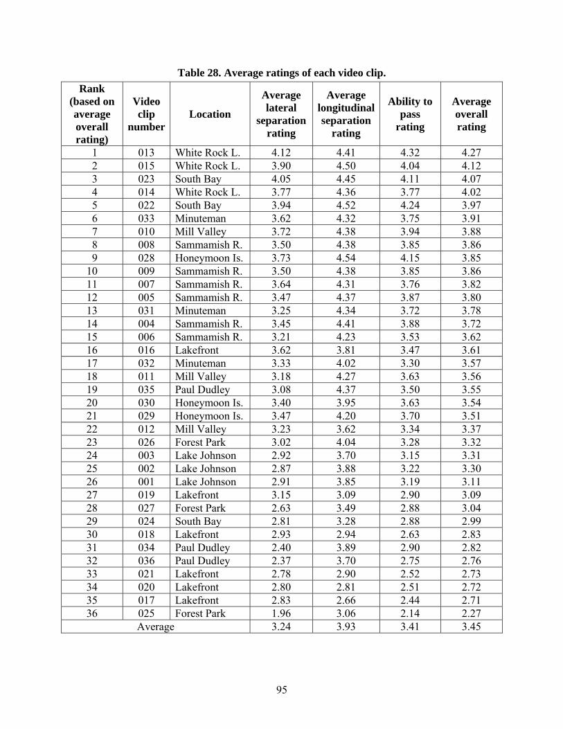
95

Table 28. Average ratings of each video clip. Rank

(based on average overall rating)

Video clip

number Location

Average lateral

separation rating

Average longitudinal separation

rating

Ability to pass

rating

Average overall rating

1 013 White Rock L. 4.12 4.41 4.32 4.27 2 015 White Rock L. 3.90 4.50 4.04 4.12 3 023 South Bay 4.05 4.45 4.11 4.07 4 014 White Rock L. 3.77 4.36 3.77 4.02 5 022 South Bay 3.94 4.52 4.24 3.97 6 033 Minuteman 3.62 4.32 3.75 3.91 7 010 Mill Valley 3.72 4.38 3.94 3.88 8 008 Sammamish R. 3.50 4.38 3.85 3.86 9 028 Honeymoon Is. 3.73 4.54 4.15 3.85 10 009 Sammamish R. 3.50 4.38 3.85 3.86 11 007 Sammamish R. 3.64 4.31 3.76 3.82 12 005 Sammamish R. 3.47 4.37 3.87 3.80 13 031 Minuteman 3.25 4.34 3.72 3.78 14 004 Sammamish R. 3.45 4.41 3.88 3.72 15 006 Sammamish R. 3.21 4.23 3.53 3.62 16 016 Lakefront 3.62 3.81 3.47 3.61 17 032 Minuteman 3.33 4.02 3.30 3.57 18 011 Mill Valley 3.18 4.27 3.63 3.56 19 035 Paul Dudley 3.08 4.37 3.50 3.55 20 030 Honeymoon Is. 3.40 3.95 3.63 3.54 21 029 Honeymoon Is. 3.47 4.20 3.70 3.51 22 012 Mill Valley 3.23 3.62 3.34 3.37 23 026 Forest Park 3.02 4.04 3.28 3.32 24 003 Lake Johnson 2.92 3.70 3.15 3.31 25 002 Lake Johnson 2.87 3.88 3.22 3.30 26 001 Lake Johnson 2.91 3.85 3.19 3.11 27 019 Lakefront 3.15 3.09 2.90 3.09 28 027 Forest Park 2.63 3.49 2.88 3.04 29 024 South Bay 2.81 3.28 2.88 2.99 30 018 Lakefront 2.93 2.94 2.63 2.83 31 034 Paul Dudley 2.40 3.89 2.90 2.82 32 036 Paul Dudley 2.37 3.70 2.75 2.76 33 021 Lakefront 2.78 2.90 2.52 2.73 34 020 Lakefront 2.80 2.81 2.51 2.72 35 017 Lakefront 2.83 2.66 2.44 2.71 36 025 Forest Park 1.96 3.06 2.14 2.27

Average 3.24 3.93 3.41 3.45

96

Demographic Variables An exploration of the demographic variables that we collected on the respondents showed that these variables generally had little effect on the score that the respondents provided. The next few paragraphs illustrate the general point. Figure 21 shows how respondent age affected the “overall” score they provided. The video clip rank corresponds to that provided in table 30 (i.e., clip 1 was from the White Rock Lake path and had the highest average “overall” score of the 36 clips). The plotted lines correspond to four age groups, and there were at least 20 respondents in each group. Obviously, the lines track each other very closely. The 32- to 45-year-old age group generally provided the highest scores, the 46- to 58–year-old age group generally provided the lowest scores, and the other age groups fell between those two. However, except for that shift in average score, respondents of different ages generally perceived the differences between two video clips to be about the same.

2.0

2.5

3.0

3.5

4.0

4.5

5.0

1 6 11 16 21 26 31 36

Video clip by overall rank

Mea

n ov

eral

l sco

re

Age 18-31 years Age 32-45 yearsAge 46-58 years Age 59 years and older

Figure 21. Effects of respondent age on overall rating. Figures 22 through 25 show lines similar to figure 21, except that the variables graphed are respondent gender, mode of travel (bicyclist versus pedestrian), health status, and trail use. Again, the pattern for all of these cases is that there were shifts from one group of respondents to another; however, respondents of different groups generally perceived the differences between two video clips to be about the same. In figure 22, we see that men generally provided higher scores than women. In figure 23, it appears that respondents from a pedestrian point of view provided generally higher scores than respondents from a bicyclist point of view. From figure 24, we note that those reporting themselves to be in fair health provided generally lower scores than those reporting themselves to be in good or excellent health. Finally, figure 25 shows no clear

97

trend in ratings by the reported amount of trail use. Overall, these respondent demographic variables seem to matter regarding the score magnitude, but they do not seem to interact with the information on the video image of the path.

2.0

2.5

3.0

3.5

4.0

4.5

1 6 11 16 21 26 31 36

Video clip by overall rank

Mea

n ov

eral

l sco

re

Male Female

Figure 22. Effects of respondent gender on overall rating.

98

2.0

2.5

3.0

3.5

4.0

4.5

5.0

1 6 11 16 21 26 31 36

Video clip by overall rank

Mea

n ov

eral

l sco

re

Bicyclist Pedestrian

Figure 23. Effects of path user type on overall rating.

2.0

2.5

3.0

3.5

4.0

4.5

5.0

1 6 11 16 21 26 31 36

Video clip by overall rank

Mea

n ov

eral

l sco

re

Excellent Good Fair

Figure 24. Effects of respondent health status on overall rating.

99

2.0

2.5

3.0

3.5

4.0

4.5

5.0

1 6 11 16 21 26 31 36

Video clip by overall rank

Mea

n ov

eral

l sco

re

A few times a year More than once a monthMore than twice a week Almost daily

Figure 25. Effects of respondent path use on overall rating.

Path Design Variables A look at the relationship between path width and respondent rating shows that path width should probably be an important variable in an LOS model. Figure 26 plots path width against mean overall rating for each of the 36 video clips. The ratings appear to be generally heading upward as the path width rises from 2.4 to 4.2 m (8 to 14 ft). For the 6.1-m- (20-ft-) wide trail video clips (from the Lakefront Trail in Chicago), the average ratings fall back down; however, that may be a result of the very heavy volumes and numbers of events shown during those clips rather than the path width. A similar relationship is seen between the path width and the average rating of the lateral separation perceived by the respondents.

Table 29 summarizes the responses for other key path design variables, including the presence of a centerline, the width of clear zone extending laterally from the edge of the path, and the forward sight distance along the path. The table shows average overall ratings for all of the video clips that have a particular level of a variable and average ratings for either lateral separation or the ability to pass, depending on which of those was more relevant for that variable.

100

2.0

2.5

3.0

3.5

4.0

4.5

5.0

8 10 12 14 16 18 20

Path width, feet

Mea

n ov

eral

l rat

ing

1 ft = 0.305 m

Figure 26. Effects of path width on overall rating.

The presence of a centerline seems to be strongly related to the overall rating—paths with no centerline rated, on average, about 0.1 points better than did paths with dashed centerlines, and about 0.4 points better than did paths with solid centerlines. This may be a result of the perceived restrictions in freedom to maneuver the bicycle imposed by a centerline. Clear-zone width does not seem to have a strong or consistent relationship with average overall rating, or with the average rating of lateral separation. Finally, while paths with poor sight distances were generally rated lowest overall and for the ability to pass, improvements in sight distance above poor did not produce consistently improving ratings. Events on the Path Respondents were not in a very good position to judge the volume of traffic on the paths in the video clips since they only viewed 1-min time slices from a moving-bicyclist perspective. However, the advantage of the moving-bicyclist perspective was that we were able to convey the number of events during that minute—the meetings and passings—quite realistically. Figure 27 shows the relationship between meetings during the 1-min clip, and average overall rating, while figure 28 relates the number of active passings and the average overall rating. Both figures suggest that average ratings decline as the number of meetings and active passings rise, with the decline for active passings being a bit more pronounced. The project team had concerns for both of these graphs in the sense that the Chicago path, with its relatively large number of meetings, average overall rating, and active passings, was dominating the results from the other paths. This concern will be addressed in the next section, which describes the detailed statistical modeling of these results.

101

Table 29. Effects of other path design variables on average ratings. Variable Level Average overall

rank Average lateral separation rank

Average ability to pass rank

No 3.61 3.35 – Dashed 3.49 3.21 –

Presence of centerline

Solid 3.23 3.13 – 0 and 5* 3.63 3.53 –

1 3.05 2.62 – 2 3.24 2.90 – 3 3.76 3.40 – 4 2.88 2.53 – 6 3.60 3.38 – 8 3.78 3.46 – 15 4.13 3.93 –

Clear zone, feet

20 3.19 3.21 – Poor 3.05 – 2.93 Fair 3.76 – 3.59

Good 3.48 – 3.45

Sight distance

Unlimited 3.76 – 3.81 *The path shown in these video clips had, on average, no clear zone on one side and 1.5 m (5 ft) on the other side.

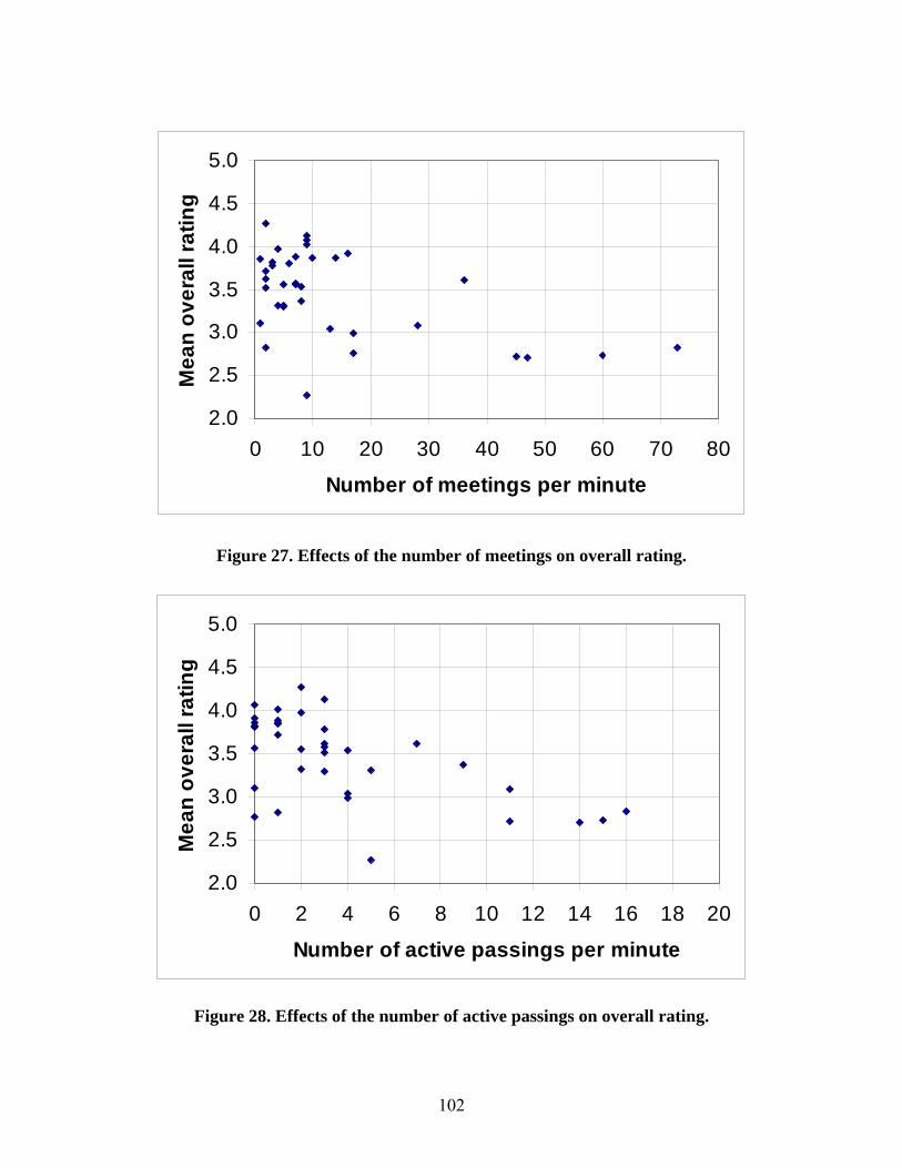
102

2.0

2.5

3.0

3.5

4.0

4.5

5.0

0 10 20 30 40 50 60 70 80

Number of meetings per minute

Mea

n ov

eral

l rat

ing

Figure 27. Effects of the number of meetings on overall rating.

2.0

2.5

3.0

3.5

4.0

4.5

5.0

0 2 4 6 8 10 12 14 16 18 20

Number of active passings per minute

Mea

n ov

eral

l rat

ing

Figure 28. Effects of the number of active passings on overall rating.

103

Video Quality The final category of perception data variables that the project team analyzed was the quality of the video. As stated earlier, we chose to show the respondents videos shot from the moving-bicyclist perspective during the operational data collection in order to portray real paths with real traffic loads. However, the downside of this approach was that the quality of the video varied from quite good to quite poor. Three important qualities that captured this variability were amount of glare, quality of the focus, and amount of vertical tilt since all of these were judged by the project team. Table 30 shows how these varied in the average overall rating provided by the respondents. None of the three quality variables had a strong relationship with average overall rating. Only the glare variable appeared as if it might matter during detailed modeling efforts since the average overall rating for the video clips with no glare was higher than for video clips with some glare; however, as the amount of glare increased from low to medium to high, the average overall ratings did not continue to decline. It appears from table 30 that the respondents were able to rate the paths according to other criteria aside from video quality.

Table 30. Effects of video quality on average ratings. Variable Level Number of video

clips Average overall

rating No 11 3.73 Low 12 3.39 Medium 5 3.18

Glare

High 8 3.33 In focus 21 3.32 Slightly out of focus 11 3.68 Moderately out of focus 3 3.39

Focus

Highly out of focus 1 3.91 None 16 3.39 Small tilt 6 3.68 Moderate tilt 10 3.41

Vertical tilt

Large tilt 4 3.45

104

MODEL CREATION Interactions The basic statistical model was based on a two-way layout that considered both subject characteristics and trail characteristics without interaction between the two. Below is the basic model:

(57)

where:

ijy = Service rating for a trail i by a subject j μ = Intercept

iα = Effect of trail characteristics jβ = Effect of subject characteristics

ije = Error The interaction of subject characteristics and trail characteristics could be a potentially complicating factor in this experiment setup. The simplification brought on by excluding such an interaction has great value; moreover, the validity of the analysis would be suspect if strong interactions were present. The experiment setup precluded any replication—no subject had multiple ratings of the same video or trail under the same conditions. While the full subject-by-trail interaction could not be addressed in this model, we did look for interactions between subject characteristics and trails, and trail characteristics and subjects.

In the case of subject characteristics, the appropriate model was as shown in equation 58:

(58) where yij, µ, αi, and eij are as defined above; k represents the response variables; and zjk represents the subject characteristics. Testing for interactions meant creating models and then examining them for the presence of (αη)k. We examined the following subject characteristics—age, gender, pedestrian or bicycle point of view, and fitness level. As we suspected from the data we examined earlier in this chapter, none of these interactions proved to be sizeable. In the case of trail characteristics, the appropriate model was as shown in equation 59:

(59)

ij i j ijy eμ α β= + + +

∑∑ ++++=k

ijjkkk

jkkiij ezzy )(αηηαμ

∑∑∑ +++++=k

ijikkj

k

ikk

k

ikkij exxwy )(βδβδθμ

105

where yij, µ, βj, k, and eij are as defined above; wik represents traffic-load variables such as meetings and passings; and xik represents the trail and location characteristics. Testing for interactions meant constructing a model and then looking for the presence of (βδ)k. We tested for trail pavement material, shoulder presence, shoulder width, shadow in the video, glare in the video, horizontal curvature, vertical curvature, sight distance, urban versus other environment, presence of a centerline, and average clear-zone width. The greatest interactions were found with the pavement material, presence of a shoulder, and urban versus other environment, with F-statistics in these cases as large as 4.87, 3.93, and 3.54, respectively. However, practically speaking, these were not very important interactions in a database of more than 3,500 observations. The modest size of these interaction effects, coupled with the ineffectiveness of these three variables as explanatory variables in subsequent modeling (see below), gave sufficient support for excluding these interactions from the model. While the respondents were sampled from a relevant population, this sample may not be representative of some shared paths at some times, and adjustments to the model may be needed in those cases. If the characteristics of the users of a path of interest were different from those of our respondents in terms of age, gender, etc., the lack of interaction seen with these variables in trial models dictates that the effect of these changes in respondent characteristics would only make an additive shift in the ratings, and will not change the relationship with the trail characteristics. Averaging over subjects leads to the following refinement from equation 59: (60)

where all variables are as previously defined, and the overbars and dots are reminders that we are averaging over the second subscript (respondents). The mean of the random subject effect, β , will be subsumed by the intercept, µ, as we fit the model to the data. It is important to note with this model that the variance of the error, var( .ie ), is now substantially reduced because it is divided by the number of respondents, i.e., σ2/N. Inclusion of this random respondent effect only affects forecasting for a new sample of respondents, and only through its mean, β , with a substantially smaller variance than it would have otherwise. Choice of Overall Response Since we asked for responses for four different ratings of each video clip, we had to choose which to use in our model of quality of service of the path. We chose to create a model using the overall rating for two primary reasons. First, table 31, which provides the correlations among all the responses fit from a preliminary modeling effort using equation 48 above, shows that the responses were highly correlated among the four perception measures or responses. In fact, the overall rating was the most highly correlated with the other perception measures. Furthermore, the overall rating was designed to capture the respondents’ feelings with regard to all aspects of the path scene that they were viewing; however, the other perception measures honed in on more specific aspects. For example, lateral separation will probably capture the respondents’ feelings about path width, but not about the sight distance ahead on the path. For these reasons, the model development that follows is concentrated on the overall rating provided by the respondents.

∑∑∑ +++++=k

iikkk

ikkk

ikki exxwy .. )( βδβδθμ

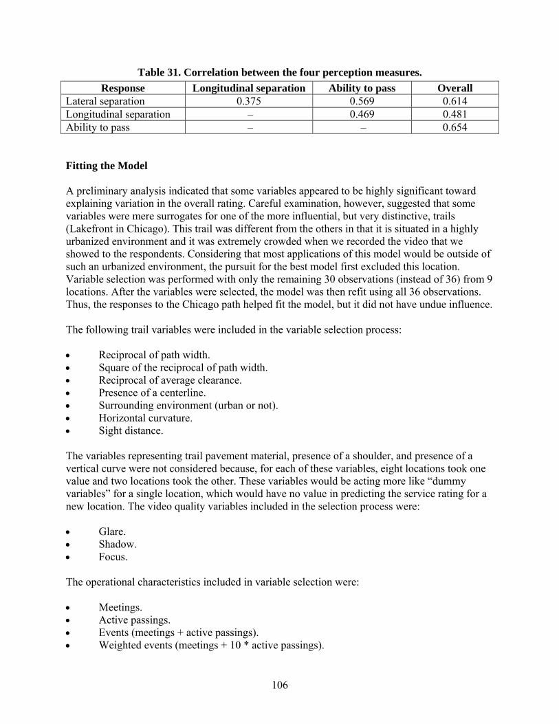
106

Table 31. Correlation between the four perception measures. Response Longitudinal separation Ability to pass Overall

Lateral separation 0.375 0.569 0.614 Longitudinal separation – 0.469 0.481 Ability to pass – – 0.654 Fitting the Model A preliminary analysis indicated that some variables appeared to be highly significant toward explaining variation in the overall rating. Careful examination, however, suggested that some variables were mere surrogates for one of the more influential, but very distinctive, trails (Lakefront in Chicago). This trail was different from the others in that it is situated in a highly urbanized environment and it was extremely crowded when we recorded the video that we showed to the respondents. Considering that most applications of this model would be outside of such an urbanized environment, the pursuit for the best model first excluded this location. Variable selection was performed with only the remaining 30 observations (instead of 36) from 9 locations. After the variables were selected, the model was then refit using all 36 observations. Thus, the responses to the Chicago path helped fit the model, but it did not have undue influence. The following trail variables were included in the variable selection process: • Reciprocal of path width. • Square of the reciprocal of path width. • Reciprocal of average clearance. • Presence of a centerline. • Surrounding environment (urban or not). • Horizontal curvature. • Sight distance. The variables representing trail pavement material, presence of a shoulder, and presence of a vertical curve were not considered because, for each of these variables, eight locations took one value and two locations took the other. These variables would be acting more like “dummy variables” for a single location, which would have no value in predicting the service rating for a new location. The video quality variables included in the selection process were: • Glare. • Shadow. • Focus. The operational characteristics included in variable selection were: • Meetings. • Active passings. • Events (meetings + active passings). • Weighted events (meetings + 10 * active passings).

107

• Events per foot width of trail. • Weighted events per foot width of trail. Note that the factor of 10 weighting the number of active passings was constructed by fitting equation 60, not including the effect of the location characteristics. Other weightings were considered, but a weight of 10 fit best for all four response variables. A different weighting for the heavily traveled Lakefront Trail was considered and abandoned for the sake of simplicity. Because the number of potential explanatory variables exceeded the number of locations by a factor of nearly two, forward selection was employed in the model selection process. The following variables were consistently useful as explanatory variables, leading to models with high R2-values: • Reciprocal of path width (in feet). • Weighted events. • Weighted events per foot width of trail. • Presence of a centerline. • Glare. • Focus. The investigation using 9 of the 10 locations (excluding Lakefront) led to a model that used the first 4 explanatory variables (the glare and focus variables were dropped out of the running). Including the responses to the six Lakefront video clips led to nearly the same quality of fit, and most of the coefficients were not substantially different. However, the variable for the weighted events per foot width of trail did not contribute. Dropping that variable led to a simpler model with approximately the same fit. Therefore, our recommendation as the model that best predicted the overall rating (on our 1 to 5 scale) was: (61) where: E = Weighted events per min (meetings + 10 * active passings) RW = 1 / path width (in feet) CL = Presence of a centerline (0 if no, 1 if yes) Tables 32 and 33 show the analysis of variance and parameter estimate tables for this model from our statistical software (SAS). The output shows that the model fit the data well, with a high F-value that was highly significant. The R2-value for this model was a healthy 0.64, and the adjusted R2-value was also good at 0.61. The model should be easy to employ by path designers and analysts, with just three variables, two of which are under the designer’s direct control and a third which is available from the methods described in chapter 3. The negative signs of the weighted events and width variables are as expected. The sign of the centerline variable is probably a result of feeling restricted by bicyclists on a path with a centerline, particularly under the relatively low-volume conditions depicted on most of the video clips. The standard error and t-values for the intercept and each of the variables showed that they were all significantly

Overall Rating = 5.446 –0.00809(E) –15.86(RW) – 0.287(CL)

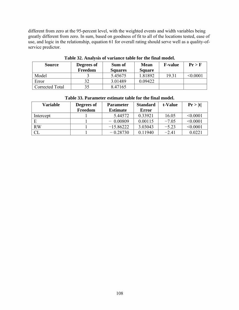
108

different from zero at the 95-percent level, with the weighted events and width variables being greatly different from zero. In sum, based on goodness of fit to all of the locations tested, ease of use, and logic in the relationship, equation 61 for overall rating should serve well as a quality-of-service predictor.

Table 32. Analysis of variance table for the final model. Source Degrees of

Freedom Sum of Squares

Mean Square

F-value Pr > F

Model 3 5.45675 1.81892 19.31 <0.0001 Error 32 3.01489 0.09422 Corrected Total 35 8.47165

Table 33. Parameter estimate table for the final model.

Variable Degrees of Freedom

Parameter Estimate

Standard Error

t-Value Pr > |t|

Intercept 1 5.44572 0.33921 16.05 <0.0001 E 1 − 0.00809 0.00115 −7.05 <0.0001 RW 1 −15.86222 3.03043 −5.23 <0.0001 CL 1 − 0.28730 0.11940 −2.41 0.0221

109

8. LOS PROCEDURE INTRODUCTION The previous chapters have shown how the study team gathered the raw materials needed to fulfill the objective of the research—a new LOS procedure for shared-use paths. The necessary literature is gathered in chapter 2, the theory is developed in chapter 3, the operational data is collected in chapters 4 and 5, and the perceptions of the path users are in chapters 6 and 7. In this chapter, we bring all this together to propose, justify, and demonstrate the use of the new method. Note that much of the information in this chapter is also in the User’s Guide that accompanies this report. This chapter contains more technical detail on the development of the procedure, while the User’s Guide contains more practical information for the user, such as case study applications of the procedure; however, much of the information is common to both. The new LOS procedure is intended primarily for trail planners, designers, and managers, which include professionals from a wide variety of disciplines (e.g., planners, landscape architects, transportation engineers, bicycle and pedestrian transportation specialists, and park and recreation planners and managers). It may also be useful for trail, bicycle, and pedestrian advocates; elected officials; planning and park commissioners; and other members of the public, especially those individuals who find themselves involved in trail planning efforts or situations involving trail user conflicts that stem from high volumes and diverse mode mixes. These conditions are increasingly common on trails located in urban, suburban, and high-use recreational areas. The LOS procedure can be used for a variety of trail planning tasks where quantitative evaluation is needed to assist in solving design or management problems, including: • Planning of appropriate widths and cross sections for new trails. • Evaluation of the LOS provided on existing trails. • Guiding of the design of improvements for existing trails where additional capacity is

needed. • Determination of how many additional users a trail may be able to serve given a

minimum LOS threshold. • Evaluation of the LOS for specific timeframes when particular trip purposes need to be

served, such as weekday mornings and evenings when commuting trips are heaviest. • Determination of the LOS at a particular location on a trail, such as a narrow pinch point,

in an unusually high-use area, or in an area with many reported user conflicts.

110

TYPES OF SHARED-USE PATHS TO WHICH THIS STUDY APPLIES Readers of this report may understand the term shared-use path (or multi-use trail) to be applicable to a very wide range of facility types and settings. It is important to note that the LOS procedure introduced in this chapter was not developed to be applicable to every type of shared-use path. The list below describes the limits of the study and the specific applicability of its findings: • The procedure is applicable only to paved hard surface paths (asphalt or concrete). Paths

surfaced with gravel, dirt, wood chips, or other materials were not evaluated in the research. Surface type and quality is not a component of this LOS evaluation.

• The procedure evaluates path LOS in terms of bicycle mobility. While the findings and

recommendations will probably improve a trail’s conditions for all users (pedestrians, joggers, inline skaters, etc.), the study was conducted from the point of view of the bicyclist.

• The tool does not accommodate the use of specific mode-split inputs for users outside the

five user groups identified in chapter 5 (i.e., adult bicyclists, pedestrians, joggers, inline skaters, and child bicyclists). Moreover, it is not applicable to situations that seek to evaluate the unique impact on LOS that other trail users may have, such as push scooters, wheelchair users, equestrians, cross-country skiers, electric vehicles, or others who may be a part of the mix on some trails.

• This tool is not applicable to trail segments that have stop signs, signal controls, or road

crossings more frequently than every 0.40 km (0.25 mi). • The tool is structured to address two-way, shared-use path facilities. It was not created

with bicycle-only or one-way paths in mind; however, it may be applicable to paths of this nature. It does not apply to on-street bicycle facilities.

LOS DEFINED For motor vehicles on roadways, the HCM defines LOS as a quality measure describing operational conditions within a traffic stream, generally in terms of such service measures as speed and travel time, freedom to maneuver, traffic interruptions, and comfort and convenience.(4) The HCM defines six levels of service for any particular facility type and uses letters from A through F to represent them (from best to worst). Each LOS represents a range of operating conditions. Although there has been some discussion of this in the literature, safety is not included in the measures that establish motor vehicle service levels. The trail LOS procedure developed through this research is similar to that used for motor vehicle LOS. These similarities include: • The shared-use path LOS procedure uses six levels of service categories (letters A

through F, representing best to worst).

111

• Maintaining an optimum speed (for the bicyclist) is a key criterion. • The service measures are primarily related to the concept of freedom to maneuver;

specifically, they include meetings, active passings, and delayed passings. • Safety is not included in the set of measurements that establish service levels. However, there are some key differences, including that the trail LOS does not factor in travel time or traffic interruptions such as signals or stop signs at grade crossings. It is important to note that there are a host of other factors that the reader may think are important to consider in a trail user’s assessment of comfort and enjoyment of a trail, such as: • Pavement/surface condition and materials. • Weather. • Frequency and design of curves. • Presence and degree of grade changes (hills). • Proximity to adjacent motor vehicle traffic. • Quality of scenery. • Physical setting. • Quality of bicycling equipment in use. • Perceived safety of the surrounding neighborhood. Just as motor vehicle LOS measures a limited aspect of the experience of driving (it does not take into account the quality of the vehicle in which a person travels, the scenery along the road, etc.), the trail LOS model measures a limited aspect of the experience of bicycling on a trail. While other factors of trail design are also important to the user’s experience, those factors will be left to further research. THE PERCEPTION SURVEY RESPONSE SCALE The LOS procedure is based primarily on the perception survey responses documented in chapter 7. The 105 respondents provided a rating of each video clip on a scale of 1 (poor) to 5 (excellent). Since this is the best current data set on path user perceptions, the research team wanted to ensure that the LOS scale corresponded with this response scale as closely as possible. Table 34 shows how we made this correspondence. We placed the midpoint of the LOS scale, at the C/D boundary, at the midpoint of the response scale (3.0). The extreme levels of service, A and F, accounted for larger parts of the response scale because the respondents tended to cluster their responses toward the middle values (i.e., relatively few respondents scored any video clip as a 1 or a 5).

112

Table 34. Correspondence between perception score and LOS. Overall Perception Score LOS

X > 4.0 A 3.5 < X < 4.0 B 3.0 < X < 3.5 C 2.5 < X < 3.0 D 2.0 < X < 2.5 E X < 2.0 F

In general, A through C can be considered above-average levels of service, and D through F as below-average levels of service, compared to the opinions of the respondents viewing scenes from 10 trails across the United States. The LOS descriptions that follow are based on the experiences of the research team, may provide a more refined framework for trail designers and planners. A benefit of this LOS framework is that it provides a uniform quantitative measurement for use throughout the United States and North America. However, there is certainly latitude for each political jurisdiction and trail managing agency to adopt differing policies about which scores and grades will be regarded as acceptable levels of service for trails within their own communities, as is the case with roadway levels of service. To some degree, determining what scores and grades are acceptable can vary in each different application of the model. For example, a jurisdiction may elect to establish a policy to ensure that new trails meet a higher performance standard than that which is considered acceptable for existing trails. In general, A through C can be considered above-average levels of service, and D through F as below-average levels of service, compared to the opinions of the respondents viewing scenes from 10 trails across the United States. The LOS descriptions below, based on the experiences of the research team, may provide a more refined framework for trail designers and planners.

A: Excellent. Trail has optimum conditions for individual bicyclists and retains ample space to absorb more users of all modes while providing a high-quality user experience. Some newly built trails will provide A-level service until they have “been discovered,” or until their ridership builds up to projected levels. B: Good. Trail has good bicycling conditions and retains significant room to absorb more users while maintaining an ability to provide a high-quality user experience. C: Fair. Trail has minimum width to meet current demand and to provide basic service to bicyclists. A modest level of additional capacity is available for bicyclists and skaters; however, more pedestrians, joggers, or other slow-moving users will begin to diminish the LOS for bicyclists. D: Poor. Trail is nearing its functional capacity given its width, volume, and mode split. Peak-period travel speeds will probably be reduced by levels of crowding. The addition of more users of any mode will result in significant service degradation. Some bicyclists

113

and skaters will probably be adjusting their experience expectations or avoiding peak-period use. E: Very Poor. Given trail width, volume, and user mix, the trail has reached its functional capacity. Peak-period travel speeds will probably be reduced by levels of crowding. The trail may enjoy strong community support because of its high usage rate; however, many bicyclists and skaters will probably be adjusting their experience expectations or avoiding peak-period use. F: Failing. Trail is popular to the point of significantly diminishing the experience for at least one, and probably all, user groups. It does not effectively serve most bicyclists; significant user conflicts should be expected.

A benefit of this LOS framework is that it provides a uniform quantitative measurement for use throughout the United States and North America. However, there is certainly latitude for each political jurisdiction and trail managing agency to adopt differing policies about which scores and grades will be regarded as acceptable levels of service for trails within their own communities, as is the case with roadway levels of service. To some degree, determining what scores and grades are acceptable can vary in each different application of the model. For example, a jurisdiction may elect to establish a policy to ensure that new trails meet a higher performance standard than that which is considered acceptable for existing trails. DEVELOPING THE LOS PROCEDURE The research team embarked on the task of assembling an LOS procedure with several key objectives in mind. The procedure should: • Be based on the operational and perception data from the previous chapters as much as

possible (meaning that it had been based on recent field data from U.S. paths and users). • Be in conformance with the scale presented in table 34 above. • Use inputs that are easy to assemble for the typical trail planner or designer. • Have a logical calculation that could be explained to the public and to decisionmakers. • Have a calculation that could be completed quickly in a spreadsheet or similar format. • Have clear and unambiguous output. • Include all possible grades (A through F), depending on the user volume (i.e.,

continuous). The next few sections describe the procedure we developed to meet these objectives.

114

Start With the Model from Chapter 7 Our LOS procedure starts with the model of perception survey responses that emerged from chapter 7. That model was:

(61[repeated]) where: E = Weighted events per min = meetings per min + 10 * active passings per minute RW = Reciprocal of path width (i.e., 1 / path width (in feet)) CL = 1 if the trail has a centerline, 0 if the trail has no centerline The researchers recommend using the spreadsheets described in chapter 3 to compute the number of meetings and passings per minute needed for equation 61. The spreadsheets from chapter 3 were based on the best current traffic-flow theory, and were validated reasonably well against field data in chapter 5. The number of meetings and passings is difficult to compute by hand, since the calculation must be repeated many times over small slices of the path; however, it lends itself to an efficient spreadsheet computation. The inputs into the meetings and passings calculation include one-way volumes of each user group, mean and standard deviation of the speed of each user group, and the “propensity to pass” factor discussed in chapter 3. Planners and designers should have at least some notion of the volumes they expect on a path to be analyzed; and most planners and designers will be content using default values (based on solid research) for the other inputs under most circumstances. Model Does Not Cover All Combinations Applying equation 61 directly with the LOS scale in table 34 proved to be troublesome, however, because the model was not sensitive enough under low-volume or high-volume conditions. Table 35 illustrates the difficulty. Table 35 basically covers the range of volumes shown to the perception survey respondents. Average values of mode split, PHF, and directional split were applied, and the computation assumed no centerline on the paths. The levels of service in table 35 are based on the scale in table 34 being applied to the score computed from equation 61. For 2.44-m (8-ft) paths, an LOS of A or B is impossible, and for 3.05-m (10-ft) paths, an LOS of A is impossible. At the other extreme, for a 4.88-m (16-ft) path, one-way flow rates above 1,600 users per hour is needed to get an LOS of F; even on a 3.66-m (12-ft) path, a one-way flow rate of 1,400 users per hour leads only to an LOS of E. The reason for the lack of sensitivity in the result from equation 61 is probably because respondents did not see enough video clips at the extreme combinations of volume and path width. For example, we did not show any clips from 2.44-m (8-ft) paths with very high volumes, or wide paths with very low volumes. We would have liked to have shown such clips to the respondents; however, we did not record any of these in the field.

LOS Score = 5.446 – 0.00809(E) – 15.86(RW) – 0.287(CL)

115

Table 35. Scores and levels of service based only on equation 61. 8-ft-wide

path 10-ft-wide

path 12-ft-wide

path 16-ft-wide

path One-way flow rate,

users/h

Meetings per hour

Passings per hour Model

score LOS Model

score LOS Model

score LOS Model

score LOS

0 0 0 3.47 C 3.86 B 4.13 A 4.46 A 10 27 8 3.45 C 3.85 B 4.11 A 4.44 A 20 54 16 3.44 C 3.84 B 4.10 A 4.43 A 30 81 24 3.42 C 3.82 B 4.09 A 4.42 A 40 107 32 3.41 C 3.81 B 4.07 A 4.40 A 50 134 40 3.40 C 3.79 B 4.06 A 4.39 A 60 161 48 3.38 C 3.78 B 4.04 A 4.37 A 70 188 56 3.37 C 3.76 B 4.03 A 4.36 A 80 215 64 3.35 C 3.75 B 4.01 A 4.34 A 90 242 72 3.34 C 3.73 B 4.00 B 4.33 A 100 268 80 3.32 C 3.72 B 3.98 B 4.31 A 200 537 160 3.18 C 3.58 B 3.84 B 4.17 A 300 805 240 3.04 C 3.43 C 3.70 B 4.03 A 400 1074 320 2.89 D 3.29 C 3.55 B 3.88 B 500 1342 400 2.75 D 3.14 C 3.41 C 3.74 B 600 1611 480 2.60 D 3.00 C 3.26 C 3.60 B 700 1879 560 2.46 E 2.86 D 3.12 C 3.45 C 800 2148 640 2.32 E 2.71 D 2.98 D 3.31 C 900 2416 720 2.17 E 2.57 D 2.83 D 3.16 C 1000 2685 800 2.03 E 2.43 E 2.69 D 3.02 C 1100 2953 880 1.88 F 2.28 E 2.55 D 2.88 D 1200 3222 960 1.74 F 2.14 E 2.40 E 2.73 D 1300 3490 1040 1.60 F 1.99 F 2.26 E 2.59 D 1400 3759 1120 1.45 F 1.85 F 2.11 E 2.44 E 1500 4027 1200 1.31 F 1.71 F 1.97 F 2.30 E 1600 4296 1280 1.17 F 1.56 F 1.83 F 2.16 E

1 ft = 0.305 m DELAYED PASSING ADJUSTMENT One way in which to respond to the difficulty illustrated in table 35 would be to adjust the LOS scale to something other than that shown in table 34. However, the research team was very reluctant to change the scale because the respondents to the perception survey had provided absolute responses. They told us what the average path looked like by scoring it as a 3.0, and, by definition, that should correspond to the LOS C/D boundary. Also, the researchers wanted to keep the scale symmetrical in the sense that LOS C covered the same range of scores as LOS D, B covered the same as E, and A covered the same as F. In addition, shifting the scale one way to allow, for instance, LOS A to cover lower scores, would have helped for narrow paths, but would have made the situation untenable for wider paths, where LOS A would have then applied to

116

paths that were quite busy. The research team thought about establishing different scales for different path widths; however, that would be awkward to implement and would again violate the spirit of the respondent survey in that the respondents had supplied answers regarding paths of widths from 2.44 to 6.1 m (8 to 20 ft) on one scale. Rather than adjust the scale, the researchers looked for an important factor that was not included in the perception survey and, therefore, had no chance to be reflected in equation 53. This factor was the number of delayed passings—the times in which the test bicyclist had to slow down before passing a slower path user traveling in the same direction. Delayed passings were not included in the perception survey (there was virtually no opportunity for respondents to view one of those cases). Yet, the researchers had good reason to include these delayed passing cases in the process, including the fact that bicyclists despised delayed passings because of the wasted time and the energy needed to regain the desired speed. In addition, there are similar factors defining LOS in other facets of highway capacity, including the two-lane highway chapter. The assumption that no passings are delayed is one of the key criticisms of the shared-path LOS methodology in the 2000 HCM.(4) Chapter 3 showed how delayed passings may be calculated and provided a spreadsheet for the calculation. Inputs for the calculation include user volumes by mode, PHF, directional split, mean speeds, the number of lanes, the proportion of users occupying two lanes, and the distance needed for the test unit to pass one of the five other modes. Most of these inputs are the same as for equation 61. The number of lanes did not figure into the perception survey result in equation 61; however, some assumptions will be needed for this calculation. For this procedure, the researchers recommend that: • Paths from 2.44 to 3.20 m (8 to 10.5 ft) wide operate as two-lane paths. • Paths from 3.35 to 4.42 m (11 to 14.5 ft) wide operate as three-lane paths. • Paths from 4.57 to 6.1 m (15 to 20 ft) wide operate as four-lane paths. These widths roughly correlate with the AASHTO Guide for the Development of Bicycle Facilities’ recommended 1.2-m (4-ft) minimum allocation of space for safe bicycle operation.(1) These widths also matched what the research team generally observed during its operational data collection effort on 15 trails across the United States. The proportion of users occupying two lanes, and the distance needed for the test unit to pass one of the five other modes, will be based on the data provided in chapter 5. A major question was how to integrate delayed passing into the perception survey model (equation 61) in order to eliminate the issues noted above in table 35, without creating new problems. The researchers investigated basing LOS on both the score from equation 61 and on an estimate of the number or percentage of delayed passings—in a manner similar to that in the two-lane highway chapter (chapter 20) in the 2000 HCM.(4) However, basing an LOS on two criteria introduces the possibility of discontinuities (cases when the LOS might skip from A to C, for instance, with the addition of just one user). To account for delayed passings without introducing potential discontinuities, the researchers introduced another factor to equation 61:

117

Overall Rating = 5.446 – 0.00809(E) –15.86(RW) – 0.287(CL) − (DP) (62)

where E, RW, and CL are as defined above; and DP is the delayed passing adjustment. After examining a number of possibilities, the researchers decided on a maximum DP of 1.5, which corresponds to, at most, three levels of service. Since the range of delayed passings per hour was from about 1 to 180 per hour (using the spreadsheets from chapter 3 and the average values of needed inputs), the researchers recommended that the delayed passing adjustment be a linear function covering this range or: (63) where DP is as defined above, and DPPH is the number of delayed passings per hour from the spreadsheet produced in chapter 3. The application of the delayed passing adjustment, as described above, makes the LOS procedure much more sensitive to higher volumes, while avoiding discontinuities. The inputs are reasonable and the calculation is easy using the spreadsheet that we developed. Tables provided later will show the effect that the delayed passing adjustment had on the LOS for various paths. Adjustment for Low Number of Events To address the difficulty noted above, that for narrow paths, levels of service of A or B are not possible, the research team introduced a low-volume adjustment as follows: • All paths with a number of weighted events per minute of five or below are scored as

LOS A. • All paths with a number of weighted events per minute from just over 5 to 10 are scored

as LOS B, unless they were otherwise going to earn an LOS A grade based on equation 62.

The researchers chose those levels to ensure that every LOS was possible at every trail width studied, from 2.44 to 6.1 m (8 to 20 ft). The levels of these adjustments are rather modest. Five weighted events per minute, with average mode splits and other assumptions, means a flow rate of about 30 one-way users per hour, while 10 weighted events per minute mean a flow rate of about 60 one-way users per hour. Putting It All Together With the delayed passing adjustment in place to remove the difficulties at high volumes, and the low-volume adjustment in place removing those difficulties, the LOS procedure is complete. In step-by-step form, the recommended LOS procedure is: 1. Compute the number of meetings per minute using the spreadsheet from chapter 3. 2. Compute the number of active passings per minute using the spreadsheet from chapter 3.

DP = DPPH * 1.5 / 180

118

3. Combine the meetings and active passings from steps 1 and 2 into an estimate of weighted events per minute by multiplying the active passings by 10 and adding that result to the meetings.

4. Compute the number of delayed passings per hour using the spreadsheet from chapter 3. 5. Convert the estimate of delayed passings per hour into the delayed passing adjustment

factor using equation 63. 6. Using the path width, the presence of a centerline, and the results from steps 3 and 5,

compute the LOS score from equation 62. 7. Use table 34 to convert the LOS score from step 6 into a tentative LOS grade. 8. Apply one of the low-volume adjustments given above if the number of weighted events

per minute is 10 or lower to find the final LOS grade. The recommended procedure meets all of the objectives laid out at the beginning of the chapter: • It is largely based on the operational and perception data from the previous chapters,

including the perception survey responses at the heart of the procedure. • It conforms to the scale presented in table 34 above. • The inputs are easy to assemble for the typical trail planner or designer. • The calculation is logical and could be explained to the public and to decisionmakers. • The calculation can be completed quickly in a spreadsheet. • The procedure produces a single LOS grade (as clear and unambiguous an output as

possible). • All LOS grades are possible at each path width studied. Table 36 shows the effects of the delayed passing adjustment and the low-volume adjustment on the same combinations of volume and path width as examined in table 35 for the unadjusted model. The low-volume adjustment changed the LOS grade for the first six rows in the 2.44-m (8-ft) column and the first three rows in the 3.05-m (10-ft) column from C to A or B. The weighted passing adjustment tended to change the LOS above about 100 one-way users per hour by one or two levels.

119

Table 36. Scores and grades based on complete LOS procedure. 8-ft-wide

path 10-ft-wide

path 12-ft-wide

path 16-ft-wide

path One-way flow rate,

users/h

Meetings per hour

Passings

per hour

Model score*

LOS Model score*

LOS Model score*

LOS Model score*

LOS

0 0 0 3.47 A 3.86 A 4.13 A 4.46 A 10 27 8 3.45 A 3.84 A 4.11 A 4.44 A 20 54 16 3.42 A 3.81 A 4.10 A 4.43 A 30 81 24 3.38 B 3.78 B 4.08 A 4.41 A 40 107 32 3.33 B 3.73 B 4.06 A 4.39 A 50 134 40 3.28 B 3.68 B 4.03 A 4.36 A 60 161 48 3.23 C 3.62 B 4.01 A 4.34 A 70 188 56 3.17 C 3.56 B 3.98 B 4.32 A 80 215 64 3.10 C 3.50 C 3.95 B 4.29 A 90 242 72 3.04 C 3.43 C 3.92 B 4.26 A 100 268 80 2.97 D 3.36 C 3.88 B 4.23 A 200 537 160 2.21 E 2.61 D 3.44 C 3.86 B 300 805 240 1.54 F 1.93 F 2.82 D 3.40 C 400 1074 320 1.39 F 1.79 F 2.09 E 2.85 D 500 1342 400 1.25 F 1.64 F 1.91 F 2.26 E 600 1611 480 1.10 F 1.50 F 1.76 F 2.10 E 700 1879 560 0.96 F 1.36 F 1.62 F 1.95 F 800 2148 640 0.82 F 1.21 F 1.48 F 1.81 F 900 2416 720 0.67 F 1.07 F 1.33 F 1.66 F 1000 2685 800 0.53 F 0.93 F 1.19 F 1.52 F 1100 2953 880 0.38 F 0.78 F 1.05 F 1.38 F 1200 3222 960 0.24 F 0.64 F 0.90 F 1.23 F 1300 3490 1040 0.10 F 0.49 F 0.76 F 1.09 F 1400 3759 1120 0.00 F 0.35 F 0.61 F 0.94 F 1500 4027 1200 0.00 F 0.21 F 0.47 F 0.80 F 1600 4296 1280 0.00 F 0.06 F 0.33 F 0.66 F

* Before low-volume adjustment. 1 ft = 0.305 m Comparison to HCM Method The recommended new procedure will return different LOS values than the LOS method in the 2000 HCM(4) for a given path. (4) Figure 29 shows a comparison of the recommended new method to the LOS method in the 2000 HCM for a 2.44-m- (8-ft-) wide (two-lane) path with no centerline, while figure 30 shows a comparison for a 3.66-m- (12-ft-) wide (three-lane) path with no centerline. In both comparisons, all other variables are at their average or default values. Both figures show LOS values for the 2000 HCM method in two different ways: (1) considering meetings and passings of bicycles and pedestrians only, and (2) considering meetings and passings of all path users by the test bicyclist.

120

0 100 200 300 400 500

One-Way Volume, Users per Hour

Leve

l of S

ervi

ce

New Procedure HCM Bike and Ped. OnlyHCM All Users

A

D

B

C

E

F

Figure 29. Comparison of recommended new LOS procedure to 2000 HCM procedure for a 2.44-m- (8-ft-) wide (two-lane) path with no centerline.

Figures 29 and 30 both show that the new LOS procedure is more optimistic than the 2000 HCM method. The difference is typically one LOS, until the new procedure predicts LOS F; however, it was as high as three levels of service for 3.66-m- (12-ft-) wide paths at 200 one-way users per hour. The differences in LOS predictions probably result from the generally optimistic ratings of the video clips provided by the perception survey respondents.

121

0 100 200 300 400 500

One-Way Volume, Users per Hour

Leve

l of S

ervi

ce

New Procedure HCM Bike and Ped. OnlyHCM All Users

A

D

B

C

E

F

Figure 30. Comparison of recommended new LOS procedure to 2000 HCM procedure for a 3.66-m- (12-ft-) wide (three-lane) path with no centerline.

APPLYING THE MODEL The LOS procedure is applicable to a variety of trail planning and design problems related to crowding and accommodating diverse user groups. It is especially useful for trail planning and design tasks that need to augment qualitative criteria with quantitative measures in order to strengthen the basis for making trail design decisions. To enable the model to be easily used by practitioners, it has been programmed into a spreadsheet tool. This tool is called the Shared-Use Path Level of Service (SUPLOS) Calculator and it accompanies this report. This section helps the reader understand how to apply this tool effectively and to generate results that are appropriate for the particular problem at hand. To make the best use of the Calculator, it is important to understand the limits of its application, and how contextual factors should be considered when collecting or structuring the input data. Link Analysis The LOS procedure is a link analysis tool. It is designed to provide an LOS evaluation for a particular link or segment of a linear trail. It is not designed to evaluate trail/roadway intersections, rest stops, or trailheads. In general, segment length is not a limiting factor in selecting a link for analysis.

122

The key to determining how much trail can be evaluated with one calculation is whether or not the trail conditions and use characteristics remain the same over the entire length that has been selected. However, because of the distance assumptions used in the model, trail segments under 0.4 km (0.25 mi) are not recommended for analysis. Moreover, because typical trip distances for some trail users are limited, and user turnback rates will begin to undermine the accuracy of the volume and mode-split data on longer segments, 3.2 or 4.8 km (2 or 3 mi) is a recommended maximum segment length. Each practitioner needs to exercise professional judgment in making these decisions. To assist in that effort, the following list of conditions and characteristics should remain roughly the same over the entire distance of trail that is being considered as one link (segment): • Trail width. • Trail user volume. • Trail user mix (mode split). • Presence of a centerline stripe. • Absence of significant flow interruptions such as stop signs, signalized road crossings, or

other grade crossings. • Absence of spur trails, trailheads, or other access points that may significantly affect user

volumes or mix. If any of these characteristics change significantly over the length of a trail segment, it is recommended that the segment be divided into one or more links using road crossings, access points, or other locations where characteristics change as endpoints for the smaller segments. Moreover, when considering establishing a trail volume and user mix profile for a single segment that is longer than 1.6 km (1 mi), based on counts taken in only one location, it is important to determine if turnback rates for pedestrians or for other users might be significant enough to affect the accuracy of these data for the sections of the segment that are farthest from the data collection point. In other words, if users often turn around partway through a segment, a single count may not represent the whole segment very well. As with any model, the quality and accuracy of the output can be no better than that of the inputs. It is understood that the quality and accuracy of input data will vary for each user of the tool. Moreover, each user and/or situation does not demand a uniform level of accuracy to produce a useful result. For these and other reasons, professional judgment is critical in determining what level of accuracy is required for the data to be used in any particular application. In most situations, slight variations in data may not affect LOS scores significantly, and the tool itself can be used to test variations in data and to determine what impact they do have on LOS results. The LOS procedure does not factor in the potential delay and other impacts of stop signs, signalized road crossings, or other grade crossings that interrupt the flow of trail traffic. The model is designed to generate LOS scores for trail segments of 0.40 km (0.25 mi) or longer, with no flow interruptions. If LOS is desired for a length of trail that includes these types of interruptions, it should be segmented at these locations and, if possible, separate volume and mode-split data should be developed for each segment. Segments shorter than 0.40 km (0.25 mi)

123

are generally dominated by the stop signs or signals at the ends; consequently, a segment LOS would not normally be appropriate for those places. Data Requirements Only four data inputs are needed to generate an LOS estimate: (1) trail width, (2) presence of a centerline, (3) one-way user volume, and (4) mode split. The following discussion of data requirements is provided to help readers apply the tool correctly and effectively to their unique situations. Trail Width Trail width should be measured in feet. Widths may be entered in half-foot increments (i.e., 8.0, 8.5, 9.0, etc.) (1 ft = 0.305 m). The procedure was calibrated on data from trails that had widths between 2.4 and 6.1 m (8 and 20 ft). Widths greater or less than these amounts will produce LOS outputs; however, the model is not designed to address widths outside of the 2.4- to 6.1-m (8- to 20-ft) range. Centerline Centerline is a “yes/no” input to be based on the existing striping pattern of each segment or the proposed striping pattern for an unbuilt trail.

Trail User Volume The volume data needed for the procedure can be provided in one of three ways, depending on how the tool is being applied: 1)By using actual volume counts collected on an existing trail, 2) by using estimated volume counts developed by extrapolating from actual volume data gathered on another trail that is determined to be similar to the test trail (this can be one of the trails addressed in this study), or 3) the “average trail” described in the User’s Guide. or By developing projected user volumes, such as for an unbuilt trail, where LOS calculations will be used to aid in the trail planning and design process. Whether volume data are developed from estimates or actual counts, they should be structured, or restructured, in the following ways: • A one-way trail volume should be calculated for each separate segment (link) of trail for

which an LOS score is desired. If counts are structured as total two-way volumes, an assumed 50/50 directional split is recommended for conversion to one-way volumes. Volume data should be in, or converted to, users per hour.

• Volume data should include a total count of all user types (modes) that use the treadway

being evaluated. If there is a separate parallel treadway in the same trail corridor, such as a jogging track or equestrian trail, users on this treadway should not be included in the volume or in the user mix data used in the model.

124

• If new user counts are collected for use in this tool, it is recommended that a minimum of three hourly, two-way counts be taken for each trail segment for which an LOS score is desired. For each test trail segment, an average, per hour, one-way volume can be created from the three hourly, two-way counts.

Mode Split Mode split is expressed as a percentage of one-way trail users per hour. The model provides the opportunity to input a mode-split percentage for up to five different modes: adult bicyclists, pedestrians, joggers, inline skaters, and child bicyclists. In the calculation tool, mode-split inputs can be round numbers or precise numbers using one decimal place, and they need to add up to 100 percent exactly. Zero is an acceptable entry for any mode. Given the entire set of user types that are found on shared-use paths, these five categories were developed based on the actual users that were observed on the 15 study trails. Other users, such as push scooters, electric scooters (used by disabled persons), wheelchairs, etc., may be present or expected on trails where this tool is applied. If the mode-split data being used for the test trail segment include a breakout of user percentages in categories other than the five used by the Calculator, add that percentage to whichever one of the five modes has the closest corresponding travel speed. Average travel speeds by mode for each of the five modes listed above were presented in chapter 5, and are also in the User’s Guide. If actual mode splits are not known and estimates need to be developed, users can: • Use mode splits from data gathered on another trail in the community or region that is

sufficiently similar to the trail to be analyzed. • Use the mode split for the average trail (i.e., the average mode split for the 15 trails for

which operational data were collected during this research, presented in chapter 5). This can be accomplished by clicking a button in the Calculator spreadsheet labeled default mode split.

• Review the mode splits of the 15 study trails from this research (see chapter 5 or the

User’s Guide) and use a mode split from one of the study trails judged to be similar to the trail to be analyzed (i.e., the trail is located in a similar community, has a similar setting, has a similar width, etc.).

On many trails, user volumes and mixes will vary considerably along different segments of the facility. When more accurate LOS scores are desired, trail segmenting should take these variations into account. The following is a list of spatial and behavioral factors that can generate significant volume and mode-split fluctuations, and which can be used to guide segmentation:

• Locations of trail access points, including junctions with other trails, spur trails,

trailheads, park nodes along a trail, and access points between the trail and adjacent trip generators and destinations.

125

• Trip generators and destinations associated with points of access, such as housing developments, employment centers, schools, parks, university campuses, entertainment attractions, or other institutions or public properties.

• Typical trip lengths and turnback rates. These will vary by user type and from trail to trail

because they are influenced by a number of trail-specific factors, such as trail layout, trip purposes, landscape character, and the personal habits and needs of local trail users.

Additionally, when new user counts are planned, these factors may be used to inform the location, frequency, and timing of the counts. When volume and mode-split estimates are being used for model inputs, these factors may be used to make adjustments to the estimates to increase the accuracy. Effects of Temporal Factors Temporal factors (e.g., season of the year, day of the week, and time of day) may be the most significant factors affecting trail user volumes. Therefore, any LOS estimate applies only to the timeframes in which the volume data counts were taken. In most cases, trail analysts seek to understand trail operations under fully loaded conditions. When this is the case, the volume data to be used in the Calculator should reflect those conditions. The volume data should be gathered during (or adjusted to reflect) the typical highest use times. The exact number and duration of user counts that are needed to fully describe fully loaded conditions may vary from case to case, depending on the level of detail desired for the volume profile and on how the resulting LOS score is to be used. To be consistent with the data collection methods used on the 15 trails studied in this project and to ensure some statistical stability in the results, at least three 1-h counts are recommended for each trail segment evaluated. Assuming that the purpose of the LOS score is to determine whether, and how, to improve service during high-use periods, counts should be taken during the high-use season, on high-use days, at high-use times of the day. In some cases, the crux of a trail manager’s problem may center as much around determining the duration or extent of high-use periods as it does around determining how bad levels of service get during high-use times. In other words, if poor levels of service are only experienced a few weekends a year, or for an hour or two on a weekend day, it may be more tolerable than if a trail is crowded all day long throughout the spring, summer, and fall. In this way, the duration of time over which a certain LOS applies may be as important to know as the LOS score itself. In these cases, the volume data that are used in the Calculator will need to be more extensive and reflect greater temporal diversity. Some users of this tool may seek an LOS evaluation for a more specific purpose, such as to determine what the LOS is for bicycle commuters during the afternoon peak. In such a case, the data would need to be gathered on weekdays, during the season(s) that generate the highest commuting rates, and would focus on the particular afternoon hours when bicyclists are present on the trail segments in question.

126

Assumptions and Default Values The following are the key assumptions and default values built into the Shared-Use Path LOS Calculator. These are generally based on average values from the data we collected during this project on 15 representative trails scattered across the United States. Users with significant departures from these values can change them in the Calculator. Directional Split The Calculator assumes a 50/50 directional split. User Speed The Calculator uses the average speeds and standard deviations for each user group, as shown in chapter 5. The default speed for the test bicyclist is 20.61 km/h (12.8 mi/h), the same speed as that of the average bicyclist. Peak-hour Factor The Calculator uses a default PHF of 0.85. This factor was calculated using the data collected on the study trails and was based on the peak 15 min, as is the custom in the HCM. The model applies the PHF of 0.85 to the one-way, per hour, user volume, which results in a volume boost of 17.6 percent. This factor ensures that the model results are responsive to the typical peak flow conditions that are found on trails. Number of Lanes This and other trail research has found that bicyclists on trails tend to operate in distinct lanes, whether or not the lanes are indicated on the trail surface with striping. Typical patterns include two-lane, three-lane, and four-lane operations:

• On two-lane operations, passing maneuvers are made in the opposing lane. • On three-lane operations, each direction of travel shares use of a “middle” lane for

passing maneuvers. • On four-lane operations, each direction of travel has its own passing lane.

Because there are no existing universal standards that correlate trail width with lane operations, this study assumed the following for the LOS procedure: • Paths from 2.44 to 3.20 m (8 to 10.5 ft) wide operate as two-lane paths. • Paths from 3.35 to 4.42 m (11 to 14.5 ft) wide operate as three-lane paths. • Paths from 4.57 to 6.1 m (15 to 20 ft) wide operate as four-lane paths. These widths roughly correlate with the AASHTO Bicycle Facility Design Guide’s recommended 1.22-m (4-ft) minimum allocation of space for safe bicycle operation.(1) These

127

widths also match what the research team generally observed during its operational data collection effort on 15 trails across the United States. Lane configuration matters only in the calculation of the delayed passing factor. The Calculator automatically determines the correct lane configuration to be used based on trail width. The delayed passing factor is computed differently for each of the three possible lane configurations, using the overall trail volume, mode split, and average travel speeds, to calculate the probability of encountering delay in a passing maneuver:

• Two-lane operations have the greatest potential for creating delayed passings because the

bicyclist must use the opposing lane to pass a slower user, and that lane may be occupied by users traveling in the opposite direction.

• Three-lane operations provide the bicyclist with better conditions for passing slower

users because of the presence of a center, shared passing lane. Delay is determined primarily by the likelihood that a trail user traveling in the opposite direction is using the center lane to make a passing maneuver; thus, there is less likelihood of delay.

• Four-lane operations provide even better passing conditions because the probability of a

delayed passing maneuver is greatly reduced, unless overall user volume is extremely high.

LOS LOOKUP TABLES Appendix C of the User’s Guide includes a series of lookup tables that provide LOS estimates for a variety of combinations of volume, mode split, and trail width, based on default values for other variables. Instructions for Using the LOS Calculator The Shared-Use Path Level of Service Calculator is provided in the form of a spreadsheet. It has the complete LOS model programmed into it, and provides a one-page, user-friendly interface (worksheet) that allows the user to analyze up to five data sets at a time. The Calculator requires only four inputs to generate an LOS estimate from the bicyclist perspective—trail width, presence of a centerline, trail user volume, and mode split—for up to five user types (adult bicyclists, pedestrians, joggers, inline skaters, and child bicyclists). The Shared-Use Path Level of Service Calculator should be opened in Excel. “Enable Macros” should be selected in the first dialogue box. If it is not already selected, the SUP_LOS_ Calculator tab at the bottom of the window should be selected. This will open the Calculator worksheet. Before beginning the data entry process, review the previous discussion about data requirements. Based on that discussion, assemble the data necessary to conduct the analysis. • The first column provides a cell to enter the trail or segment name. Type in a name or

segment identifier.

128

• The second column provides a cell for the trail width. Enter a number representing the desired width in feet. Widths may be entered in half-foot increments (i.e., 8.0, 8.5, 9.0, etc.) (1 ft = 0.305 m).

• The third column asks if the trail has (or will have) a centerline. Type in a “1” for yes or a

“0” for no. • The fourth column provides a cell for one-way trail volume per hour. Enter a number. • Columns five through nine provide cells for mode split. Entries may or may not use

decimal increments in tenths. The sum of the five mode splits must total exactly 100, or an error message will appear above the data entry row.

• Data entries cannot be made in any of the spreadsheet cells, other than those described

above. Once all of the numeric inputs are provided, columns 11 and 12 will calculate the level of service score and will provide the level of service grade, automatically. In the upper right-hand corner of the spreadsheet, a scale is provided that correlates scores with the grade. In general, grades A through C can be considered above-average levels of service, and grades D through F as below-average levels of service. Once the LOS has been computed, the whole sheet may be copied or printed to a word or spreadsheet file to create a permanent record of these cases and results. Once the information has been pasted into a new file, revision of model calculations will not be possible in that new document. The results may be printed using the regular print commands to print directly from Excel, or by printing the file to which copies have been saved. By copying and saving the results to another file, the Calculator can be used over and over again without losing the results of previous scenarios. For convenience, the Calculator worksheet has been designed with a separate one-click button to reset the default mode split for each row.

129

Implications for Trail Design The central findings of this study have important implications for trail design. The following is a list of key findings that can be used to inform design choices: • Width is the key factor in determining LOS, and every additional foot of trail width has a

positive impact on LOS, according to the model. • Bicyclists’ LOS on pathways is very sensitive to user mix; when the amount of foot

traffic (joggers and pedestrians) surpasses the 15 percent trail level, the level of service is significantly impacted.

• Bicyclists are responsive to the use of a centerline stripe to divide directional flows. Trail Width The LOS procedure provides strong support for the standard trail-width guidance provided in the AASHTO Guide for the Development of Bicycle Facilities.(1) Trails that are 2.4 m (8 ft), which AASHTO recommends only in “rare instances,” were found to have poor levels of service, except at very low volumes, or with user mixes that included few pedestrians and joggers. The findings of this research supports AASHTO’s(1) minimum “recommended paved width for a two-directional shared-use path of 10 feet [3 m].” The procedure shows that widths of 3.35 to 4.57 m (11 to 15 ft) provide improved levels of service for higher volumes and more balanced user mixes. This is also consistent with AASHTO recommendations that, “under certain conditions, it may be necessary or desirable to increase the width of a shared-use path to 12 ft [3.6 m], or even 14 ft [4.2 m], due to substantial use by bicycles, joggers, skaters, and pedestrians.”(1) Trails of 3.35 to 4.57 m (11 to 15 ft) are wide enough to operate as three-lane paths. The increased passing capacity provided by a trail that operates as three lanes improves LOS and increases the trail’s ability to absorb higher volumes and more diverse mode splits without severely degrading service. The implications for designers of these results regarding trail width include: • During design of new trails and widening of existing trails, designers may want to

consider varying the trail width to achieve LOS goals in key locations while not “overbuilding” in other locations. Adding width to improve LOS is valuable to trail users, even if it is provided only on selected segments.

• When considering wider trails, designers and decisionmakers may want to think in 0.305-

m (1-ft), rather than in 0.61-m (2-ft), increments. Typical practice has been to consider trail widths in 0.61-m (2-ft) increments (i.e., 3.05, 3.66, 4.27 m (10, 12, 14 ft), etc.). This approach may lead designers to miss opportunities to provide measurable increases in LOS, while at the same time, containing costs and minimizing environmental impacts.

130

Centerline Striping A striped centerline was found to have a strong impact on the bicyclist’s perception of freedom to maneuver. This finding appears to support the intent of trail designers in providing a centerline, which is to clearly delineate two opposing travel lanes. A centerline reinforces the idea that to pass a slower moving user, the bicyclist may need to use the travel lane of opposing trail users, and should pass only when the opposing lane is open. This research found that the presence of a centerline stripe results in a significant reduction in the LOS score. It appears that bicyclists felt less comfortable making a same-direction passing movement when a centerline stripe was present. While this finding might appear initially to mean that a centerline should not be used, it is important to note that there may be other valid safety reasons for providing a centerline stripe, particularly on crowded trails, on curves with limited sight distance, and in other appropriate circumstances. Only two trails in this study were striped with more than two travel lanes. The Pinellas Trail near Saint Petersburg, FL, was striped as a three-lane trail, one in each direction for bicycles and skaters, and one lane for pedestrians. The Lakefront Trail in Chicago, IL, was striped as four lanes, two in each direction. These two examples did not represent a sufficient number of study trails to fully assess the impact of multi-lane striping patterns on LOS. However, the LOS procedure is based on the idea that having sufficient trail width for a four-lane operation (a minimum of 4.57 m (15 ft)) increases the ability of bicyclists to pass slower moving users without encountering blockage from trail users in the opposing lanes. Multiple Treadways A number of shared-use trails have been designed with two treadways in the same trail corridor. Often, one is paved and the other is a soft surface. Frequently, one of the treadways is provided for exclusive use by one or two trail user groups, or user restrictions are imposed on both paths in an effort to segregate users. Given the impact of user mix on bicyclist LOS, a multiple treadway design that effectively reduces the number of pedestrians and joggers mixing with bicyclists will have significant LOS benefits for the treadway used by bicyclists and skaters. This study did not address compliance with use restrictions—an issue that is often raised by trail managers as a problem when separate treadways are provided. Trail Operations and Management While this study did not examine issues related to trail operations and management, the framework of the tool may lend itself to applications in this area. Ideas include using LOS grades in warrants for warning or trail etiquette signs. These trail etiquette signs address sharing of the treadway or use of designated passing protocols. The LOS procedure may also be useful in setting trail speed limits or in establishing other advisory or regulatory protocols that will increase user safety and will moderate user conflicts.

131

CASE STUDIES The User’s Guide contains several case studies posing typical problems facing designers and showing how the LOS procedure can help provide solutions to those problems.

133

9. CONCLUSIONS AND RECOMMENDATIONS

INTRODUCTION Shared-use paths are paved, off-street travel ways designed to serve nonmotorized travelers. Shared-use paths are gaining popularity in two different ways in recent years in the United States. First, there are many more paths and many more miles of paths being created. Second, shared-use paths are attracting a increasingly greater amount of use. Some urban trails attract thousands of users per hour during peak periods and some are experiencing rush hours and traffic jams. Trail managers are becoming increasingly concerned about user conflicts and injuries, and some are also concerned that potential users are deciding not to come out and use a trail because of crowding. The design of a new path or a path to be rebuilt is thus an increasingly important activity. During the design of every shared-use path, someone eventually asks, “How wide should this pathway be?” That question nearly always raises even more questions: What types of users can we reasonably expect? When will we need to widen the path? Do we need to separate different types of users from each other? These are very difficult questions for designers who face that classic design dilemma of overbuilding versus obsolescence. If the designer specifies a trail to be wider than future use justifies, there is a waste of money that could otherwise have been used to construct more miles of trail elsewhere. If the designer specifies a trail that proves to be too narrow for the future volume and mix of users, there will be more user conflicts and collisions, greater unhappiness among users, and the need to consider expensive trail widening. At the present time, conventional design manuals do little to help designers resolve their dilemmas. The classic procedure first specified by Hein Botma in The Netherlands, which bases LOS on the estimated number of meetings and passings for bicyclists, is an attractive framework that could help designers. There can be little debate that, in general, paths where bicyclists must make more meetings and passings should be less desirable than trails with fewer meetings and passings. However, the LOS procedure in the 2000 HCM(4), adapted from Botma’s work, has a number of serious limitations that make it difficult for designers to use in order to resolve their path design dilemmas. The overall project objective was the production of a tool that professionals can use to evaluate the operational effectiveness of a shared-use path, given a traffic forecast or observation at an existing path along with some geometric parameters. The project adopted Botma’s method as the basic framework for the LOS procedure. In particular, the objective was to produce a tool that overcomes the major limitations in the current LOS procedure noted above. The desired procedure emerging from this project would: • Be calibrated and validated. • Be based on U.S. data. • Have LOS criteria based on user input. • Include more modes. • Include the ability to change key parameters such as mean speeds.

134

• Account for delayed passing. • Analyze the full range of existing and possible path widths. • Be in a form ready for use by path designers. CONCLUSIONS Our four major achievements during the project included: • Development of the additional theoretical framework necessary to overcome the

limitations to the existing procedure noted above.

• Collection of field data on path operations to calibrate and validate the theoretical equations for U.S. conditions.

• Collection of path user perception data to establish LOS criteria.

• Development of an LOS estimation tool that professionals working with shared-use paths

can use and a plan to provide them with that tool. During the project, we made two significant advances in the theory of traffic flow on shared-use paths. First, we extended the previous method to other modes, other speed distributions, and passive passings. As noted, a passive passing is an occasion when the test bicyclist is passed by a faster path user. Second, the team developed a way to calculate the number of delayed passings. These are times when the test bicyclist would arrive behind a slower path user and not be able to pass because of the lack of an adequate gap in the next lane to the left (oncoming or same direction). Obviously, delayed passings are undesirable for bicyclists since they then have to slow down and then probably expend energy accelerating when an adequate gap does appear. Delayed passings are also critical because they are so highly related to path width. Prior to this project, there were some delayed passing calculations in the literature related to two-lane highway operation, etc.; however, there was nothing in the literature related to shared-path operation. Our new theory will estimate delayed passings of various modes for two-lane, three-lane, and four-lane paths. The objective of the operational data collection portion of this project was to collect the field data needed to calibrate and validate the LOS model for shared-use paths. To calibrate and validate an LOS model, the main variables that we needed to collect were meetings and desired and actual passings by path users, and the speeds and volumes of the path user groups. The team chose to use the moving-bicycle method to collect these variables. We collected a database of more than 700 runs of (mostly) 0.80 km (0.5 mi) each by our test bicyclist on 15 shared-use paths in 10 cities across the United States. The database included a wide array of volumes and speeds for five different major user groups. The major analysis of the database was to use the theory described above to predict of the number of meetings and passings for each run, and to compare that prediction to the number of meetings and passings counted in the field. Our results showed that the prediction matched the field count fairly well at most sites. We also were able to use the operational database to find the default values that we needed for the LOS procedure, and to use the videotapes for our perception data collection.

135

The third major part of this effort was to collect data on user perceptions of multi-use trail designs and operations to help set the LOS criteria. We did this by showing more than 100 volunteer respondents thirty-six 1-min videotapes of paths recorded using the helmet camera during the operational data collection effort. We selected the videotapes to represent a wide range of path designs and operations. The respondents were asked to state, on a five-point scale, how much they would enjoy using the path in four different ways: longitudinal separation, latitudinal separation, ability to pass, and overall. An analysis of the responses showed that there was a strong relationship between the number of meetings and passings and enjoyment, and that path width was the primary geometric variable that affected user perception. The user perception model that we developed from the data was the backbone of our LOS procedure. The most important accomplishment of the project team was the production of a new method to estimate the LOS for a shared-use path, based on the results from the other parts of the project. The procedure uses simple inputs that should be readily available to path designers, including one-way user volume, mode split, path width, and the presence or absence of a centerline. The procedure uses the theory that we developed and validated to predict the number of meetings and passings that will occur; it uses a number of default values based on data we collected if local values were not available. The LOS is based primarily on the model of user satisfaction that emerged from our perception study. Our model of delayed passing also plays a role in some LOS estimations. The output from the LOS procedure is a traditional A through F grade with which users can judge the performance of an existing path or a design alternative. The project team has also produced software to calculate the LOS automatically, greatly easing the burden on future users. RECOMMENDATIONS The new LOS estimation method produced during this project should be widely adopted by path designers because it provides many advantages over current methods, including: • The new method is based on sound theory. The theory (development of which is shown

in chapter 3) began with the work of Hein Botma in The Netherlands, and was extended here to include more modes, more speed distributions, passive passing, and delayed passing.

• The procedure to estimate meetings and passings has been validated for the first time in

the United States on a wide variety of trails. • The LOS method and scale has now been calibrated based on the perceptions of a sample

of U.S. users viewing videotapes of actual operations on actual U.S. paths. • The method only provides the LOS for bicycles, but does so while accounting for four

other modes, including child bicyclists, inline skaters, pedestrians, and joggers. • The method works for and was based on path widths from 2.44 to 6.1 m (8 to 20 ft).

136

• The method works for and was based on a full range of volumes, from virtually zero users in an hour to several thousand users per hour.

• The inputs to the procedure are still easy for a user to assemble (as were the inputs to the

previous procedures), and sound default values are provided for most variables. • The research team has provided easy-to-use software to make the LOS calculation. Marketing the New LOS Procedure Unlike the roadway environment, which is almost exclusively the domain of civil engineers, shared-use paths are designed by a wide variety of practitioners. Some of the most creative and unique trails in the country are the direct result of the diverse skills that these designers bring to the table. We identified three main target audiences for the marketing of our shared-use path LOS model: transportation professionals; trail designers/coordinators; and walking, bicycle, and trail advocates and organizations. Reaching each of these three groups with the results from this research will be challenging. To reach transportation professionals, the Highway Capacity and Quality of Service Committee should consider the new LOS method for inclusion in the next edition of the HCM, or as an interim release until the next edition is ready. Presentations and papers at conferences and in journals of the Transportation Research Board and the Institute of Transportation Engineers will also help. To reach trail designers and trail advocates, the LOS method and User’s Guide should be posted on FHWA’s pedestrian and bicycle Web site and on the sites of other pedestrian and bicycle information clearinghouses. The new LOS method should also be presented to the AASHTO Task Force on Geometric Design for their consideration. If they were to include it in an update of the Guide for the Development of Bicycle Facilities,(1) there would be a great likelihood that it would be widely used and accepted. In addition, presentations and papers at conferences and in the journals of the major parks and recreation societies will also be helpful. Future Research Needs The scope of the project, and therefore of the products emerging from the project, was limited in several important ways, as explained below. We recommend that future research on shared-use paths focus on erasing those limitations and otherwise extending the work conducted here. First, we recommend research to extend this work to estimate LOS from other points of view besides bicyclists. While one can easily assume that wider paths with fewer events lead to better levels of service for pedestrians and for other path users, as they do for bicyclists, the precise nature of that relationship is in doubt. We collected some user perceptions from the pedestrian point of view; however, the sample was not large and the videos that the respondents were rating, were not from the pedestrian point of view. It would be quite feasible to conduct similar user perception surveys from groups of pedestrians, inline skaters, joggers, and others by showing each group video clips and learning their reactions. It would also be possible to extend the LOS procedure to consider other modes emerging as important users on shared-use paths, such as

137

tandem bicyclists, Segways, and wheelchairs. The data on emerging path users compiled in a recent FHWA project(44) provide a good start. Second, we recommend collecting more data on high-volume and four-lane paths to put the LOS method on a more firm footing in these situations. The database collected in this project had one such path—the Lakefront Trail in Chicago, IL—and we recorded extremely heavy volumes on that path. However, there are other paths of that width in the United States, and there will be more in the future. In addition, if the current growth in path volumes continues across the United States in the next few years, there will be many more paths with Chicago-like volumes. We noted in chapter 7 that the perception data from Chicago was almost an outlier compared to the rest of the data set; we need more data from high-volume paths to fully calibrate the LOS method under those conditions. Third, we recommend a research effort to validate the delayed passing theory that we developed during this project. The number of delayed passing attempts would seem to be a natural factor in an LOS procedure, and our theory appears sound. However, we developed the theory relatively late in the project, and did not have the opportunity to show that the theory correctly estimates the number of delayed passings versus field data. In addition, none of our perception video clips showed bicyclists that had delayed passings. We need more direct evidence of how bicyclists weigh delayed passings against undelayed active passings, meetings, and other factors critical to the LOS. Fourth, we recommend a project to validate the video method of obtaining user perceptions. This could be done by comparing a sample of perceptions from viewers of videos to a sample of perceptions from people actually using the trails. Next, we heartily recommend a project to find a better LOS procedure for intersections on shared paths. The current intersection analysis procedure in the HCM(4) is like the current LOS procedure for shared-use path segments in that it is based on good logic, but is not validated against field data from the United States. This project, of course, only provided data and analysis for segments between intersections. Given the difficulty we had during this project in finding high-volume path segments of at least 0.80 km (0.5 mi) long, intersections are probably a major concern for path users across the United States. Finally, the theory estimating the number of delayed passings we developed in this project could be applied to improve the LOS procedure for two-lane highways. The current procedure in the HCM(4) is based on a series of microscopic simulation runs. It would require some field data collection; however, with some effort, our theory could be applied to two-lane highways, and a comparison to the simulation could be revealing.

139

APPENDIX A. PERCEPTION SURVEY FACT SHEET AND INFORMED CONSENT FORM

Figure 31. Fact sheet for conformed consent.

FACT SHEET You are being asked to voluntarily participate in a research study being conducted by NC State University for the Federal Highway Administration (FHWA). The study is addressing the operational characteristics of recreational paths and trails that are used by a variety of different users (for example, pedestrians, bicyclists, runners, in-line skaters, etc.). An important part of the study involves determining how someone like yourself perceives different trail conditions. For example, we want to know how the following factors affect your perception of the trail. . . factors like the degree of ‘lateral’ separation between users (that is, the distance between you and those on your right or left); the degree of ‘longitudinal’ separation (that is, the distance between you and those in front of or behind you); and users’ ability to pass other users when they want or need to.

As a volunteer in the study, you will be asked to view thirty-six, 1-minute video segments showing a range of trail conditions and users. You will experience these conditions as if you were riding a bicycle along the trail. After viewing each 1-minute segment, you will be asked to provide your perception of trail conditions in terms of (1) lateral separation, (2) longitudinal separation; and (3) ability to pass. You will also asked to give an ‘overall’ rating of the trail. You will provide these ratings using the 5-point scale shown below. When you have finished with your ratings for a particular trail condition, we will move to the next condition. There will be 36 sets of conditions in all. We’ll pause briefly after each 9 conditions .

When you and the rest of the group have finished viewing all 36 segments, we would like for you to stay for a few minutes to collect any other thoughts or perceptions you may have that you feel were not addressed by the conditions that you viewed or the scale that you used to provide your perceptions of these conditions. Your responses will remain anonymous and will not used in any way outside the context of the present study. Your signature below indicates your concurrence with the conditions of the study. At any point in time that you wish more information about the study, you can contact either Dr. Joe Hummer (NCSU) at 919-515-7733 or Ms. An Do (FHWA) at 202-493-3319. __________________________ (last name) ________ (date) last 4 digits SSN: ___ ___ ___ ___ I am participating as a: Bicyclist Pedestrian

LATERALSEPARATION

LONGITUDINAL SEPARATION

PASSING

Condition Number XXBAD POOR FAIR GOOD EXCELLENT

LATERAL SEPARATION

LONGITUDINAL SEPARATION

ABILITY TO PASS

OVERALL

141

APPENDIX B. PERCEPTION SURVEY BACKGROUND INFORMATION FORM

Shared Use Paths and Trails

Background Information

1. GENDER: MALE FEMALE 2. AGE RANGE: 18-24 25-31 32-38 39-45 46-51 52-58 59-65 over 65 3. WALKING (OR RIDING YOUR BIKE) FOR RECREATION OR FITNESS: NEVER A FEW TIMES A YEAR MORE THAN ONCE A MONTH MORE THAN TWICE A WEEK ALMOST DAILY 4. HOW OFTEN DO YOU WALK (OR RIDE YOUR BIKE) ON SHARED USE PATHS/TRAILS? NEVER RARELY OCCASIONALLY REGULARLY 1-3 TIMES A WEEK ALMOST DAILY

142

Bike or Ped Last 4 of SSN: ________ Chapel Hill, Raleigh, TRB

5. WHAT ARE YOUR MOST FREQUENT WALKING (OR BIKE RIDING) PURPOSES WHEN USING A SHARED USE PATH/TRAIL? COMMUTING TO WORK COMMUTING TO SCHOOL UTILITARIAN TRIPS TO SOCIALIZE WITH A FRIEND(S) RECREATION PHYSICAL FITNESS 6. WHAT OTHER ACTIVITIES DO YOU PARTICIPATE IN ON SHARED USE PATHS/TRAILS? WALK RUN HIKE CROSS-COUNTRY SKI IN-LINE SKATE PUSH A CHILD IN A STROLLER JOG TRAVEL WITH A DISABLED PERSON WALK A DOG OTHER (DESCRIBE) 7. IF RESPONDING AS A BICYCLIST, WHAT OTHER TYPES OF BICYCLE EQUIPMENT DO YOU USE ON A SHARED USE PATH/TRAIL? A RECUMBANT BIKE A TANDEM BICYCLE A BICYCLE TRAILER A TRAIL-A-BIKE WITH A CHILD RIDER A FOLDING BICYCLE OTHER (PLEASE DESCRIBE) 8. YOUR ESTIMATE OF YOUR OVERALL HEALTH STATUS: POOR FAIR GOOD EXCELLENT

143

APPENDIX C. SCREEN SHOTS FROM PERCEPTION STUDY VIDEO

Figure 32. Lake Johnson Trail.

Figure 33. Sammamish River Trail.

144

Figure 34. Mill Valley-Sausalito Pathway.

Figure 35 White Rock Lake Trail.

145

Figure 36. Lakefront Trail.

Figure 37. South Bay Trail.

146

Figure 38. Forest Park Trail.

Figure 39. Honeymoon Island Trail.

147

Figure 40. Minuteman Bikeway.

Figure 41. Dr. Paul Dudley Bicycle Path.

149

REFERENCES 1. American Association of State Highway and Transportation Officials, Guide for the

Development of Bicycle Facilities, Washington, DC, 1999. 2. Transportation Research Board, Highway Capacity Manual, Special Report 209, Updated

Third Edition, Washington, DC, 1997. 3. Rouphail, N., J. Hummer, J. Milazzo, II, and D. Allen, Capacity Analysis of Pedestrian

and Bicycle Facilities: Recommended Procedures for the Bicycles Chapter of the Highway Capacity Manual, Report No. FHWA-RD-98-108, FHWA, McLean, VA, 2000.

4. Transportation Research Board, Highway Capacity Manual, Fourth Edition, Washington,

DC, 2000. 5. Botma, H., and H. Papendrecht, “Traffic Operations of Bicycle Traffic,” Transportation

Research Record 1320, Transportation Research Board, Washington, DC, pp. 65–72, 1991.

6. Harkey, D., D. Reinfurt, A. Sorton, M. Knuiman, and J. Stewart, The Bicycle

Compatibility Index: A Level-of-Service Concept, Report No. FHWA-RD-98-095, FHWA, McLean, VA, 1998.

7. Landis, B.W., V.R. Vattikuti, and M.T. Brannick, “Real-Time Human Perceptions:

Toward a Bicycle Level of Service,” Transportation Research Record 1578, Transportation Research Board, Washington, DC, 1997.

8. American Association of State Highway and Transportation Officials, A Policy on

Geometric Design of Highways and Streets, Washington, DC, 2001. 9. Federal Highway Administration, Manual on Uniform Traffic Control Devices,

Washington, DC, 2003. 10. Rouphail, N., J. Hummer, J. Milazzo, II, and D. Allen, Literature Synthesis for Chapter

13, “Pedestrians” of the Highway Capacity Manual, Federal Highway Administration, McLean, VA 1998.

11. Allen, D., N. Rouphail, J. Hummer, and J. Milazzo, II, “Operational Analysis of

Uninterrupted Bicycle Facilities,” Transportation Research Record 1636, 1998, pp. 29–36.

12. Fruin, J.J., Pedestrian Planning and Design, Metropolitan Association of Urban

Designers and Environmental Planners, New York, NY, 1971. 13. Polis, A., J. Schofer, and A. Ushpiz, “Pedestrian Flow and Level of Service,” Journal of

Transportation Engineering, January 1983.

150

14. TRB, Highway Capacity Manual, Special Report 209, Updated Third Edition,

Washington, DC, 1994. 15. Knoblauch, R., M. Nitzburg, R. Dewar, J. Templer, and M. Pietrucha, Older Pedestrian

Characteristics for Use in Highway Design, Report No. FHWA-RD-93-177, Federal Highway Administration, McLean, VA, 1995.

16. Pushkarev, B., and J. Zupan, “Capacity of Walkways,” Transportation Research Record

538, Transportation Research Board, Washington, DC, 1975. 17. Roddin, M., A Manual to Determine the Benefits of Separating Pedestrians and Vehicles,

NCHRP Report 240, Transportation Research Board, Washington, DC, 1981. 18. Kirschbaum, J.B., P.W. Axelson, P.E. Longmuir, K.M. Mispagel, J.A. Stein, and D.A

Yamada, Designing Sidewalks and Trails for Access, Part II: Best Practices Design Guide, September 2001. Accessed March 23 at http://www.fhwa.dot.gov/environment/sidewalk2/pdf.htm.

19. TRB, Highway Capacity Manual, Special Report 209, Third Edition, Washington, DC,

1985. 20. Tanaboriboon, Y., and J.A. Guyano, “Level of Service Standards for Pedestrian Facilities

in Bangkok: A Case Study,” ITE Journal, November 1989. 21. Davis, D., and J. Braaksma, “Level-of-Service Standards for Platooning Pedestrians in

Transportation Terminals,” ITE Journal, April 1987. 22. Pushkarev, B., and J. Zupan, Urban Space for Pedestrians, MIT Press, Cambridge, MA,

1975. 23. Navin, F.P.D., and R.J. Wheeler, “Pedestrian Flow Characteristics,” Traffic Engineering,

June 1969. 24. Zegeer, C., et al., The National Bicycle and Pedestrian Study: Transportation Choices for

a Changing America, Report No. FHWA-RD-94-023, Federal Highway Administration, Washington, DC, 1994.

25. Northwestern University Traffic Institute, Bicycle Planning and Facility Workshop,

Evanston, IL, 1994. 26. Wilkinson, W.C., A. Clarke, B. Epperson, and R. Knoblauch, Selecting Roadway Design

Treatments to Accommodate Bicycles, Report No. FHWA-RD-92-073, Federal Highway Administration, McLean, VA, 1994.

151

27. Hunter, W.W., and H. Huang, “User Counts on Bicycle Lanes and Multiuse Trails in the United States,” Transportation Research Record 1502, Transportation Research Board, Washington, DC, 1995, pp. 45–57.

28. Niemeier, D.A., “Longitudinal Analysis of Bicycle Count Variability: Results and Modeling Implications,” Journal of Transportation Engineering, Vol. 122, No. 3, May-June 1996.

29. Miller, R.E., and M.R. Ramey, Width Requirements for Bikeways: A Level-of-Service

Approach, Report 75-4, Department of Civil Engineering, University of California, Davis, 1975.

30. Center for Research and Contract Standardization in Civil and Traffic Engineering, Sign

Up for the Bike: Design Manual for a Cycle-Friendly Infrastructure, Record 10, Ede, The Netherlands, 1994.

31. Brilon, W., “A New German Highway Capacity Manual,” Proceedings, Second

International Symposium on Highway Capacity, Volume 1, Sydney, Australia, August 1994.

32. Vagverk, S., “Chapter 10: Bicycle Traffic Facilities” (English translation), Swedish

Capacity Manual, National Swedish Road Administration, Stockholm, 1977. 33. Yang, J.-M., “Bicycle Traffic in China, Transportation Quarterly, Vol. 39, No. 1,

January 1985. 34. Directorate of Public Roads, Norwegian Public Roads Administration, City Planning for

Cycling, Oslo, December 1995. 35. Navin, F.P.D., “Bicycle Traffic Flow Characteristics: Experimental Results and

Comparisons,” ITE Journal, Vol. 64, No. 3, March 1994. 36. Homburger, W.S., Capacity of Bus Routes, and of Pedestrian and Bicycle Facilities,

Institute of Transportation Studies, University of California, Berkeley, February 1976. 37. Opiela, K.S., S. Khasnabis, and T.K. Datta, “Determination of the Characteristics of

Bicycle Traffic at Urban Intersections,” Transportation Research Record 743, Transportation Research Board, Washington, DC, 1980, pp. 30–36.

38. Federal Highway Administration, Safety and Locational Criteria for Bicycle Facilities,

User Manual, Volume II: Design and Safety Criteria, Report No. FHWA-RD-75-114, Washington, DC, 1976.

39. Lui, Y., “The Capacity of Highways With a Mixture of Bicycle Traffic,” Proceedings,

1991 International Symposium on Highway Capacity, Rotterdam, The Netherlands.

152

40. Liu, X., L.D. Shen, and F. Ren, “Operational Analysis of Bicycle Interchanges in Beijing, China,” Transportation Research Record 1396, Transportation Research Board, Washington, DC, 1993, pp. 18–21.

41. Wei, H., J. Huang, and J. Wang, “Models for Estimating Traffic Capacity on Urban

Bicycle Lanes,” presented at the 76th Annual Meeting of the Transportation Research Board, Washington, DC, January 1997.

42. Botma, H., “Method to Determine Levels of Service for Bicycle Paths and Pedestrian-

Bicycle Paths”, Transportation Research Record 1502, Transportation Research Board, Washington, DC, 1995, pp. 38–44.

43. Virkler, M., and R. Balasubramanian, “Flow Characteristics on Shared Hiking/Biking/

Jogging Trails,” Transportation Research Record 1636, Transportation Research Board, Washington, DC, 1998, pp. 43–46.

44. Landis, B.L., T.A. Petritsch, and H.F. Huang, Characteristics of Emerging Road and

Trail Users and Their Safety, Final Report, Report No. FHWA-HRT-04-103, Federal Highway Administration, McLean, VA, October 2004.

45. Botma, H., and H. Papendrecht, “Operational Quality of Traffic on a Bicycle Path,” ITE

1993 Compendium of Technical Papers, 63rd Annual Meeting, 1993, pp. 81–85. 46. Wardrop, J., “Some Theoretical Aspects of Road Traffic Research,” Proceedings of the

Institute of Civil Engineers, Vol. 12, Part 2, London, England, 1952, pp. 333–334. 47. Rouphail, N., J. Hummer, J. Milazzo, II, and D. Allen, Capacity Analysis of Pedestrian

and Bicycle Facilities: Recommended Procedures for the Pedestrian Chapter of the Highway Capacity Manual, Report No. FHWA-RD-98-107, Federal Highway Administration, McLean, VA, 2000.

48. St. John, A., and D. Harwood, TWOPAS User Guide, Federal Highway Administration,

McLean, VA, May 1986. 49. Hoban, C., R. Shepherd, and G.J. Fawcett, A Model for Simulating Traffic on Two-Lane

Rural Roads: User Guide and Manual for TRARR Version 3.2, Australian Road Research Board, Melbourne, Australia, 1991.

50. Morrall, J., and A. Werner, “Measuring Level of Service of Two-Lane Highways by

Overtakings,” Transportation Research Record 1287, Transportation Research Board, Washington, DC, 1990, pp. 62–69.

51. Federal Highway Administration, CORSIM User’s Manual, Version 1.03, Federal

Highway Administration, McLean, VA, 1997.

153

52. Innovative Transportation Concepts, LLC, VISSIM User’s Manual, Version 2.50, Corvallis, OR

53. Van Aerde, M., Integration Release 2, User’s Manual, Queen’s University, Montreal,

Quebec, 1995. 54. Homburger, W., and J. Kell, Fundamentals of Traffic Engineering, Institute of

Transportation Studies, Berkeley, California, 1988. 55. Beukers, B., “Bicycles and Mopeds as Alternative Modes of Transportation,”

Proceedings, 13th International Study Week in Traffic Engineering and Safety, Montreux, Switzerland, 1978.

56. Botma, H., H. Papendrecht, and D. Westland, Validation of Capacity Estimators Based

on the Distribution of Headways, Transportation Research Laboratory, TU Delft, The Netherlands, 1980.

57. Ferrara, T.C., A Study of Two-Lane Intersections and Crossings Under Combined Motor

Vehicle and Bicycle Demands, Report 75-5, Civil Engineering Department, University of California, Davis, December 1975.

58. Stembord, H., “Capacity Research and Applications: Country Report of The

Netherlands,” Proceedings, 1991 International Symposium on Highway Capacity, Rotterdam, The Netherlands.

59. Pécheux, K., M. Pietrucha, and P. Jovanis, “User Perception of Level of Service at

Signalized Intersections,” Preprint CD-ROM, 79th Annual Meeting of the Transportation Research Board, Washington, DC, January 2000.

60. May, A., Traffic Flow Fundamentals, Prentice Hall, Inc., Upper Saddle River, NJ, 1990. 61. Hughes, R., and D. Harkey, “Cyclists’ Perception of Risk in a Virtual Environment:

Effects of Lane Conditions, Traffic Speed, and Traffic Volume,” Proceedings, Traffic Congestion and Traffic Safety in the 21st Century: Challenges, Innovations, and Opportunities, American Society of Civil Engineers, New York, NY, 1997.