EVALUATION OF PETROPHYSICAL PROPERTIES IN THE AK FIELD …
89
i EVALUATION OF PETROPHYSICAL PROPERTIES IN THE AK FIELD OF THE NIGER DELTA PROVINCE OF NIGERIA USING INTEGRATED DATA By Philip D. Samuels A THESIS SUBMITTED TO THE AFRICAN UNIVERSITY OF SCIENCE AND TECHNOLOGY, ABUJA- NIGERIA IN PARTIAL FULFILLMENT OF THE REQUIREMENTS FOR THE DEGREE OF MASTER OF SCIENCE IN PETROLEUM ENGINEERING UNDER THE SUPERVISION OF Prof. Dr. K. Mosto Onuoha [MAY, 2013]
Transcript of EVALUATION OF PETROPHYSICAL PROPERTIES IN THE AK FIELD …

i
EVALUATION OF PETROPHYSICAL PROPERTIES IN THE AK FIELD OF THE
NIGER DELTA PROVINCE OF NIGERIA USING INTEGRATED DATA
By
Philip D. Samuels
A THESIS
SUBMITTED TO THE AFRICAN UNIVERSITY OF SCIENCE AND TECHNOLOGY,
ABUJA- NIGERIA
IN PARTIAL FULFILLMENT OF THE REQUIREMENTS FOR THE DEGREE OF MASTER
OF SCIENCE IN PETROLEUM ENGINEERING
UNDER THE SUPERVISION OF
Prof. Dr. K. Mosto Onuoha
[MAY, 2013]

ii
EVALUATION OF PETROPHYSICAL PROPERTIES IN THE
AK FIELD OF THE NIGER DELTA PROVINCE OF NIGERIA
USING INTEGRATED DATA
BY:
PHILIP D. SAMUELS
RECOMMENDED BY:
Professor K. Mosto Onuoha
[Thesis Supervisor]
Professor Godwin Chukwu
[Committee Member]
Dr. Mukhtar Abdulkadir
[Committee Member]
APPROVED BY: Professor Godwin Chukwu
[Head, Petroleum Engineering Department]
Professor Wole Soboyejo
[Provost]
[Date]

iii
DEDICATION
This thesis is dedicated to my deceased parents and the General Auditing Commission,
Republic of Liberia, respectively for their evergreen motivations which continue to rekindle the
aspiration for the attainment of higher education and for its supportive role in encouraging and
promoting academic diversification as foundation for addressing transparency and accountability
in Liberia.

iv
ACKNOWLEDGMENT
Contributions from many sources culminated into the writing and submission of this thesis for
which I am very grateful. Against this background, I am immeasurably indebted to my thesis
supervisor, Prof. Dr. K. Mosto Onuoha whose guidance landed me on the platform of
presentation. Also, it is with great honor that I accord my thesis committee members their due
recognition for their immense contributions. Without them, this work would not have been
certified. To this end, special acknowledgement goes out to Prof. Dr. Godwin A. Chukwu and
Dr. Mukhtar Abdulkadir for their inputs and directions.
The contribution of the entire faculty of the Petroleum Engineering Department is herein
acknowledged as their lecture materials were valuable assets in obtaining supportive information.
Recognition is also accorded Messr. Chidozie I. P. Dim and Nnebedum Okechukwu of the
University of Nigeria, Nsukka and Mr. Haruna Onuh of the African University of Science
and Technology, Abuja for their enormous contributions on the software applications part of
this research.
The impetus to carry out this research was drawn from the need to predict a field’s performance
by data integration. Combining seismic and well data, this work was stimulated by the need to
develop models which would enable the estimation of reservoir parameters using the appropriate
software.
To reach this stage in my pursuit of higher education, institutional and relational supports cannot
be denied. In this vein, I extend many thanks to the General Auditing Commission of the
Republic of Liberia for its continued support during the course of my studies. And
remembering the prolonged patience endured by my wife and kids during the time of my absence

v
from home, hats-off goes out to them. My wife most especially was a constant source of moral
support and encouragement.
Finally, for the many who the limitation of space cannot allow to be named in person, I seize this
opportunity to extend my heartfelt congratulations.

vi
ABSTRACT
The AK field is an oil field draining the Agbada Formation, one of the three units of the Niger
Delta Province, which started forming about 50 million years ago. Reservoirs from the AK field
are sandstones and are located in the central offshore area of the Niger Delta. The sedimentary
basin consists of thick succession of non-marine and shallow marine deposits.
Reservoir modeling is often associated with uncertainties that lead to inadequate description of
the reservoir and inappropriate prediction of field performance. Various techniques are being
developed to reliably predict reservoir properties for appropriate reservoir characterization and
field performance respectively. The reliability with which this can be achieved is tied to
validating the data acquired from one method of investigation with another. Amongst the
various methods are seismic inversion and well integration.
The case study for this research is the AK field of the Niger Delta Province. Well log data for
thirteen (13) wells and seismic volume spanning the field are collected and analyzed to predict
water saturation, porosity, permeability, shale volume and net-to-gross sand distribution. The
analysis was performed using Schlumberger-Petrel software. Multiple inter-wells data sets
acquired from well logs and seismic survey from the field were tied together to estimate
petrophysical properties.
A Geological model comprising structural and stratigraphic framework for the AK field strata
was constructed by combining data from 13 well logs and a seismic volume spanning the areal
extent of the field. The property distribution within the reservoir was achieved by employing
geostatistics - Sequential Gaussian Simulation (SGS), Variogram and trend maps.

vii
TABLE OF CONTENTS
DEDICATION............................................................................................................................................ iii
ACKNOWLEDGMENT ........................................................................................................................... iv
ABSTRACT ................................................................................................................................................ vi
TABLE OF CONTENTS ......................................................................................................................... vii
TABLE OF FIGURES ........................................................................................................................... xi
LIST OF TABLES .................................................................................................................................xiii
LIST OF EQUATIONS ........................................................................................................................ xiv
CHAPTER 1 .............................................................................................................................................. 1
INTRODUCTION ....................................................................................................................................... 1
1.1Background and Rationale ................................................................................................................... 1
1.2 Statement of the Problem .................................................................................................................... 2
1.3 Objectives ........................................................................................................................................... 3
1.4 Merit .................................................................................................................................................... 3
1.5 Research Method ................................................................................................................................ 3
1.6 Tasks Execution Schedule .................................................................................................................. 4
1.7 Overview of the Niger Delta Province of Nigeria .............................................................................. 4
CHAPTER 2 ................................................................................................................................................ 8
LITERATURE REVIEW .......................................................................................................................... 8

viii
2.1 Well Integration and Reservoir Properties .......................................................................................... 8
2.2 Sources of data Acquisition ................................................................................................................ 9
2.3 Overview of Petrophysical Properties ............................................................................................... 15
2.4 Petrophysical Correlations ............................................................................................................... 17
2.4.1 Water Saturation Correlation ..................................................................................................... 18
2.4.2 Porosity Correlation ....................................................................................................................... 23
2.4.3 Permeability Correlation ................................................................................................................ 23
2.4.4 Shale Volume Correlation .......................................................................................................... 25
2.4.5 Net-to-Gross Ratio Correlation ...................................................................................................... 25
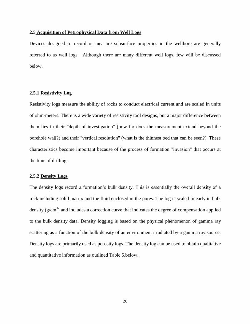
2.5 Acquisition of Petrophysical Data from Well Logs .......................................................................... 26
2.5.1 Resistivity Log ........................................................................................................................... 26
2.5.2 Density Logs .............................................................................................................................. 26
2.5.3 Sonic Log ................................................................................................................................... 27
2.5.4 Neutron Logs ............................................................................................................................. 30
2.5.5 Gamma Ray Log ........................................................................................................................ 31
2.5.6 Spontaneous Potential Log ......................................................................................................... 31
2.6 Basics of Reservoir Rock Classification ........................................................................................... 32
2.7 Application of 3D Seismic Data to Reservoir Characterization ....................................................... 33
2.8 Application of Well logs Data to Reservoir Characterization .......................................................... 34
2.8.1 Advantages and Limitations of Well Log and Seismic Data ..................................................... 35

ix
2.9 Integration of Well and 3D Seismic Data ......................................................................................... 37
2.10 Overview of the PETREL Software ................................................................................................ 38
2.10.1 The PETREL Data Types and Formats .................................................................................... 39
2.10.2 Uses of the PETREL Software ................................................................................................. 40
2.10.3 Limitations of the PETREL Software ...................................................................................... 41
CHAPTER 3 .............................................................................................................................................. 42
METHODOLOGY ................................................................................................................................... 42
3.1 Data Scope ........................................................................................................................................ 42
3.2 Data Import (Loading) Into PETREL ............................................................................................... 43
3.2.1 Order of Importing Data into PETREL .......................................................................................... 43
3.2.2 Creating Data in PETREL DATA Editor................................................................................... 44
3.2.2.1 PSpad Editor Format for Well Data ........................................................................................ 44
3.2.2.3 PSpad Editor Format for Non-Well Data (Well Tops, Seismic, Fault, Isochores etc) ............ 46
3.2.3 The Modeling Process ................................................................................................................ 48
3.2.3.1 Geo-modeling ......................................................................................................................... 48
3.2.3.2 Property Modeling .................................................................................................................. 49
CHAPTER 4 .............................................................................................................................................. 54
RESULTS AND ANALYSIS ................................................................................................................... 54
4.1 Wells Display .................................................................................................................................... 54
4.2 Well Tops Display ............................................................................................................................ 54

x
4.3 Outcome Model ................................................................................................................................ 55
4.3.1 Geological Model ....................................................................................................................... 55
4.3.2 Property Models ......................................................................................................................... 61
4.3.2.1 The Porosity Model ................................................................................................................. 61
4.3.2.2 The Water Saturation Model ................................................................................................... 62
4.3.2.3 The Shale Volume Model ....................................................................................................... 63
4.3.2.4 The Permeability Model .......................................................................................................... 64
4.3.2.5 Net-to-Gross Ratio Model ....................................................................................................... 65
4.4 Graphical Interpretation of Intra-Reservoir Properties ..................................................................... 67
CHAPTER 5 .............................................................................................................................................. 70
CONCLUSIONS AND RECOMMENDATIONS .................................................................................. 70
REFERENCES .......................................................................................................................................... 71

xi
Table of Figures
Figure 1.0: Task Execution Schedule for Thesis Implementation----------------------------------4
Figure 1.1: Diagram of the Niger Delta Province of Nigeria ---------------------------------------5
Figure 2.0: Seismic Survey Using Reflection Method----------------------------------------------11
Figure 2.1 Diagram of Density Logging Tool-------------------------------------------------------13
Figure 3.0: The well headers data file open in a PSpad window-----------------------------------44
Figure 3.1: The well path/deviation data file opened in a PSpad window-------------------------45
Figure 3.2: The well log data file for AK-001 opened in a PSpad window -----------------------46
Figure 3.3: The check shots data file open in a PSpad window-------------------------------------46
Figure 3.4: The well tops data file open in a Notepad window--------------------------------------47
Figure 3.5: Workflow for the Development of the 3D Geological Model--------------------------49
Figure 3.6: Stages in Workflow development of petrophysical models-----------------------------53
Figure 4.0: The Thirteen Wells of the AK Field Displayed in 3D Window -----------------------54
Figure 4.1: Well Tops for deviated wells Displayed in 3D Window---------------------------------55
Figure 4.2: Seismic Section with five designated faults displayed in 3D Interpretation Window---
-------------------------------------------------------------------------------------------------------------56
Figure 4.3: Fault Lines Mapped Across Seismic Section----------------------------------------------56
Figure 4.4: 3D Window display of Five Mapped Faults----------------------------------------------57

xii
Figure 4.5: Faults and Fault Polygons displayed in 3D window-------------------------------------57
Figure 4.6: Gridded Fault/ Fault Model. (Structural Model)-----------------------------------------58
Figure 4.7: Seismic section showing some major mapped horizons (Stratigraphic Tops) and
Faults with some well Bores----------------------------------------------------------------------------59
Figure 4.8: Un-Gridded Mapped Horizons (Stratigraphic/Reservoir Tops) -------------------------59
Figure 4.9: 3D Display of Surfaces constituting the formation----------------------------------------60
Figure 4.10: Geological Model Developed from Structural and Stratigraphic Frameworks------60
Figure 4.11: Porosity Model----------------------------------------------------------------------------61
Figure 4.12: Water Saturation Model-------------------------------------------------------------------62
Figure 4.13: Shale Volume Model---------------------------------------------------------------------63
Figure 4.14: Permeability Model----------------------------------------------------------------------64
Figure 4.15: Net-to-Gross Model----------------------------------------------------------------------64
Figure 4.16: Graph of Net Sand Thickness versus Depth--------------------------------------------67
Figure 4.17: Graph of Porosity versus Depth----------------------------------------------------------68

xiii
List of Tables
Table 1: Formations of the Niger Delta Province of Nigeria ........................................................ 6
Table 2: Well Logging Tools and Functions ............................................................................... 13
Table 3: Mathematical Relationships Describing Archie’s Equation .......................................... 19
Table 4: Mathematical Definition of Constants in the Generic form of the Simandoux Equation ..
..................................................................................................................................................... 22
Table 5: Types of Information obtainable from Density Log ...................................................... 27
Table 6: Wyllie’s Mathematical Formula for Determining Sonic (matrix) Porosity .................. 28
Table 7: Petrel Data Types with their File Formats, Categories, Domains and Data Editor ........ 40
Table 8: Data Categories from the AK Oil Field of the Niger Delta Province ............................. 42
Table 9: Order and Steps in Which Data are Imported into PETREL INPUT Explorer .............. 43
Table 10: Data File Types for Import to PETREL Explorer ....................................................... 44
Table 11: PSpad format for Well Path/Deviation ........................................................................ 45
Table 12: PSpad Editor Format for Well Tops and Faults .......................................................... 47
Table 13: Petrophysical Property values of the AK Field from modeling .................................. 66

xiv
List of Equations
Equation1a: Tixier Equation for Sandstone formation ................................................................ 20
Equation 2: Waxman-Smits’ Equation ........................................................................................ 20
Equation 3a: Generalized Simandoux Equation .......................................................................... 22
Equation4: Density Porosity Equation ......................................................................................... 23
Equation 5a: Generalized Rose-Wyllie Equation ........................................................................ 24
Equation 6b: Net-to-Gross Equation ............................................................................................. 25
Equation 7a:Wyllie’s Equation .................................................................................................. 29
1
CHAPTER 1
INTRODUCTION
1.1 Background and Rationale
The acquisition and handling of data play significant roles in petroleum exploration and
production. How these data can be tied together is vital to the success of exploration and
production projects. Also, the processing and interpretation of the data go a long way in
informing technical decision making and establishing the economic viability of the exploration
and production activities. For example, seismic exploration can provide information on the
subsurface structures and give tentative indication of the presence of hydrocarbon. Additionally,
information obtained from well-logs can lead to important insights on subsurface properties such
as permeability, porosity, rock types, just to highlight a few.
From seismic data generated by the reflection method using wave energy, geological structures
can be noted and the depth of seismic boundaries can be determined. For example, the reflection
method detects small angular inconsistencies, pinches, faults, traps and sections where facies
change. Well-log data can enhance predictability of formation characteristics. Well-log
measurements are performed using acoustic signals with a much broader frequency spectrum,
especially towards the higher frequencies.
Integrating both seismic and well-log data offers a good front to verify and calibrate reservoir
properties. This process of integration is called well-tying. Well integration affords the
conversion of well log measurements from depth to the time domain. Three dimensional seismic

2
acquisitions permit accessing reservoir properties over a relatively large area. Seismic attributes
are generated in the time domain.
One method by which well integration can be achieved is seismic inversion. However, this
remains outside the scope of this work. This research work illustrates how seismic and well data
can be combined using appropriate software to generate geological and petrophysical models
from seismic and well log data respectively. Also, the research focuses on establishing a trend in
the evaluation of selected petrophysical properties.
1.2 Statement of the Problem
Reservoir modelling is often associated with uncertainties that lead to inadequate description of
the reservoir and inappropriate prediction of field performance. Although the integration of well
and three dimensional seismic data is cardinal to the development of appropriate reservoir model,
the success of integration depends on the quality of the data.
Static models can be generated to estimate water saturation, porosity, permeability, volume of
shale, net-to-gross ratio, etc. These predictions should become more accurate as wells are added.
Validation of reservoir properties can be achieved by comparing numerical models with
simulation results. How the available data can be processed and imported for reservoir modelling
and how generated models are populated for reliable approximation of reservoir properties are
often challenges worth overcoming for better description and interpretation of a field’s
performance.

3
1.3 Objectives
This thesis was undertaken to achieve the following:
• Develop the appropriate geological model from structural and Stratigraphic information
• Develop the petrophysical models for reliable estimation of reservoir properties by
combining well log and 3D seismic data to determine the variations of porosity, water
saturation, net-to-gross and pore fluids in the chosen field from simulation results
• Achieve a workflow for the development of geological and petrophysical models
• Develop the appropriate petrophysical models for reliable estimation of petrophysical
properties from simulation results and ppredict field performance
1.4 Merit
With the advent of technological advances, made possible by the development of different kinds
of software to aid in prediction analysis, 3D seismic and well log data can be integrated to
generate models that describe a field’s performance thus affording predictions not far from actual
field operations.
1.5 Research Method
This research was undertaken by using real field data sets obtained from the AK Oil Field in the
Niger Delta Province of Nigeria. These data sets were quality checked (processed, imported and
filtered) to ensure software for subsurface analysis and performance prediction. Data analysis
and interpretation were conducted from simulated response pattern obtained by tying seismic and
well log data from sets of constraints employed in using the PETREL application. By

4
populating the geological model with well data, reservoir characterization was achieved for the
determination of the AK field’s performance.
1.6 Tasks Execution Schedule
For the implementation of the research, the dateline indicated below was adhered to:
Figure 1.0: Task Execution Schedule for Thesis
1.7 Overview of the Niger Delta Province of Nigeria
The Niger Delta Province includes Nigeria, Cameroon and Equatorial Guinea. The province is
situated in the Gulf of Guinea with one petroleum system, identified so far, and designated in
Nigeria as the Tertiary Niger Delta (Akata-Agbada) petroleum system. Tuttle, Charpentier and
Brownfield (1999) described the period of the formation of the Niger Delta. They outlined that
the delta formed at the site of a rift triple junction related to the opening of the southern Atlantic
Thesis Tasks Execution Schedule
Date
Activities
November
(2012)
December
(2012)
January
(2013)
February
(2013)
March
(2013)
April
(2013)
May
(2013)
Recommendation of Initial
Thesis Topic by Supervisor
Trip to Monrovia for Oil
Field Data (Request
Denied)
Return to Nigeria
Change of Initial Thesis
Topic
Compilation of Thesis
Introduction
Field Trip for Supervision
Literature Review
Field Trip for Supervision
Methodolgy
Results and Analysis
Conclusions and
Recommendations
Review by Supervisor
Review by Committee
Members
Defense
Final Review
Approval by Supervisor and
Committee MembersSubmission

5
starting in the Late Jurassic and continuing into the Cretaceous. They noted “The delta proper
began developing in the Eocene, accumulating sediments that now are over 10 kilometers thick.
The primary source rock is the upper Akata Formation, the marine-shale facies of the delta, with
possibly contribution from interbedded marine shale of the lower most Agbada Formation”.
The Niger Delta covers an aerial stretch of over 70,000 km² within the Federal Republic of
Nigeria and constitutes about one-fourteenth of the total land mass of the country. In Nigeria,
originally, the Niger Delta constituted what were then Bayelsa, Delta and River States until its
modification in the year 2000 to include a number of other states.
Figure 1.1: Diagram of the Niger Delta Province of Nigeria (Source: Internet)

6
The geologic history of the Niger Delta Province dates from Eocene period to recent times and
remains the youngest of three depositional cycles leading to the development of the coastal
sedimentary basin of Nigeria. The deposition of sediments within this period lasted from about
56 to 34 million years ago up till recent times bringing about three stratigraphic subdivisions,
namely the Benin formation, the Agbada formation and the Akata formation.
Table 1: Formations of the Niger Delta Province of Nigeria
Lithologically, the upper portion of the Niger Delta Province which makes up the Benin
formation is sandy while the middle Agbada formation comprises an intervening unit of
alternating sandstone and shale with the lower Akata formations predominantly shale.
According to Short and Stauble (1967) “These three units extend across the whole delta and each
ranges in age from early Tertiary to Recent. They are related to the present outcrops and
environments of deposition”. They further pointed out that the Tertiary section of the Niger Delta
No Formation Lithology Period of Occurence Source Depth Location
1
-Thick shale sequence
- turbidite sand
- clay and silt
2
Agbada Shale and sandstone Eocene to recent 3700 m Middle layer , major
petroleum-bearing unit
3 Benin sand Eocene to recent Alluvial and upper coastal plain 2000m Upper layer of the delta.
Akata Paleocene through
recent
Lowstands when terrestrial organic matter and
clays were transported to deep water areas
characterized by low energy conditions and
oxygen deficiency (marine Origin)
7000 m Base of the Delta

7
Province of Nigeria is divided into three litho-stratigraphic formations, representing prograding
depositional facies that are distinguished mostly on the basis of sand-shale ratios.
Tuttle, Charpentier and Brownfield (1999) investigated the hydrocarbon potential of the Niger
Delta. They noted that the “Petroleum in the Niger Delta is produced from sandstone and
unconsolidated sands predominantly in the Agbada Formation. Characteristics of the reservoirs
in the Agbada Formation are controlled by depositional environment and by depth of burial.”
Magbagbeola (2005) studied the depositional sequence of the Niger Delta and found that
Tertiary Niger Delta deposits are characterized by a series of depobelts that strike northwest-
southeast, sub-parallel to the present day shoreline. He also observed that depobelts become
successively younger basin ward, ranging in age from Eocene in the north to Pliocene offshore of
the present shoreline.
As at 1999, the Niger Delta Province of Nigeria was estimated to hold recoverable oil and gas of
around 35 billion barrels (bbl) and 94 trillion standard cubic feet (ft3) gas respectively with
production from sandstone facies within the Agbada Formation.

8
CHAPTER 2
LITERATURE REVIEW
2.1 Well Integration and Reservoir Properties
Well integration is the process of combining data from two or more distinct data sources so as to
verify and calibrate reservoir properties and predict reservoir potential. In this research work
seismic and well-log data are combined to ensure the success of well integration and good
knowledge of the subsurface. It cannot be over-emphasized that petroleum resources are found
hundreds of feet beneath the earth surface in heterogeneous formation and the precision of
information on the location of these resources rely on the understanding of the geology of the
formation.
Since the subsurface is physically inaccessible to the petroleum engineers and related
professionals, the dependence on instrument is indispensable to any determination of petroleum
resources in the subsurface. Keen understanding of the deflection pattern of instruments such as
gamma ray logging tool, density log, spontaneous potential log, just to name a few, can assist in
confirming response from seismometer on the formation properties. In this vein, the oil
industries rely on data fed to it from equipment designed to acquire data in the formation and in
comparison to those obtained from samples of formation rocks brought to the surface by the
drilling equipment for petrophysical and other laboratory analyses.
Data obtained from the propagation of waves (either refraction or reflection method) can give
clues on the formation characteristics. For example, seismic exploration techniques, based on the
study of the propagation characteristics of elastic (seismic) waves in the earth’s crust are used to
investigate the crust’s geological structure. Depending on the reflected or refracted wave signal,

9
seismologists and geologists can predict the formation rock type at various depths from arrival
time of the wave energy emitted into the formation. The wave’s arrival time is a function of the
structural or crystalline arrangement of rock atomic particles. Information obtained from the
propagated wave is used in predicting rock hardness, rock stress, rock density etc and in
classifying rock type.
Although the resolution obtained from seismic is relatively low when compared to well logging,
the area of coverage of seismic acquisition is larger than that of well-logging. Well logging on
the other hand gives high resolution but tends to be limited in that it only provides information at
the well location- the wellbore. Well-log data however include but not limited to porosity,
permeability, lithofacies, water saturation etc.
Tying seismic data to well data enables the prediction of geological ages, rock types, porosity,
and fluid types away from the well and within the well of properties such as porosity variation,
fluid types, top of abnormal pressure zones etc. from which petrophysical models can be derived.
2.2 Sources of Data Acquisition
The integration of data is at the core of reservoir modeling. The primary objective of integration
is to explicitly account for and incorporate all data necessary for describing the reservoir and
building models that approximate reality. In the petroleum industries, the principal areas from
which data can be generated are:
Seismic Survey
Well Logs (Wire line or Logging-While-Drilling)
Laboratory Analysis of Core
Others

10
While the significance of other data sources cannot be under-rated, it is however important to
state that for the purpose of this research task, emphasis would be placed on seismic survey and
well log data.
Seismic Survey: This is the process of accessing and evaluating the surface and subsurface
geology based on processed information obtained from propagated wave energy. Seismic survey
is one of the key geophysical approaches used in exploring for petroleum resources and by far
the leading and only geophysical approach used both in exploration and development phases.
Magnetic and gravity surveys, the other two geophysical approaches or methods, are used only in
pre-drilling exploration.
Seismic data can be acquired both onshore and offshore with virtually the same operational
principles but with devices adapted to each terrain. On land, for instance, acoustic waves are
generated at or near the earth surface by shooting seismic from sources such as dynamite,
thumper (a weight dropped on ground surface), dinoneis (a gas gun), or a vibroseis (which
literally vibrates the earth’s surface). The acoustic waves which are transmitted into the earth
from dynamite and the other named sources, when reflected are received by electronic devices
called geophone. Here, the geophones digitize the waves after performing a number of signal
processing stages such as amplification and filtering. The processed signals are then transmitted
to a nearby truck to be recorded on magnetic tape or disk. The recorded data sets are displayed in
a number of forms for interpretation and research purposes; including visual display forms
(photographic and dry-paper), a display of the amplitude of arriving seismic waves versus their
arrival time, and a common type of display called variable-density.

11
By utilizing information on travel time, arrival time, seismic survey provides a way of measuring
the physical properties of the subsurface formation. These measurements give geological
information which is significant in identifying structures such as faults and traps as well as
provide information on depth, stratigraphy and position of source rocks.
For offshore seismic survey, that is obtaining subsurface data by propagating acoustic waves
over marine environment, the seismic vessel replaces the on-land truck while receiver devices
called hydrophones serve the same function as the geophones which receive reflected (incoming)
signals during onshore seismic survey. Performing seismic survey offshore is cheaper
comparably to onshore due to the involvement of smaller workforce. Also the offshore process is
faster and simpler as most of the tasks are machine implemented.
Figure 2.0: Seismic Survey Using Reflection Method (Source: Internet)

12
Well Logs: To conduct formation evaluation which is also linked to the analysis of the
subsurface, wide range of measurements and geophysical techniques are required. Information
gathered through the use of calibrated instruments enables the determination of the reservoir’s
extent, pay thickness, porosity, rock type, storage capacity, hydrocarbon content, and well
produceability. Contingent on these parameters is also the determination of the economic value
and production potential of the reservoir.
Well logging provides an excellent medium for the determination of the reservoir parameters.
Well logging is the use of down-hole instrument, either during or after drilling, to evaluate the
formation and measure reservoir parameters. Log measurements, when properly calibrated, can
give the majority of the petrophysical parameters. Specifically, logs can provide a direct
measurement or give a good indication of:
Porosity, both primary and secondary
Permeability
Water saturation and hydrocarbon movability
Hydrocarbon type (oil, gas, or condensate)
Lithology
Formation dip and structure
Sedimentary environment
A single well log cannot exclusively extract all relevant data from a reservoir. Data obtained
from well logs fitted for specific activities are assimilated and utilized for the evaluation of the

13
reservoir. The table below indicates some of the most encountered well logging tools and data
each may be capable of extracting from a well:
Table 2: Well Logging Tools and Associated Data
No Well Logging Tool Data
1 Sonic Log Interval Transit Time
2 Density Log Bulk Density
3 Porosity Log Total Porosity
4 Gamma Ray Log Shale Volume
5 Resistivity Log Formation True Resistivity
Figure 2.1 Diagram of Density Logging Tool (Source: Internet)

14
Logging can answer many questions on topics ranging from basic geology to economics;
however, logging by itself cannot answer all the formation evaluation problems. Coring, core
analysis, and formation testing are all integral parts of any formation evaluation effort.
Laboratory Analysis of Core: A core is a cylindrical sample of the formation extracted from a
depth of interest for laboratory analysis. Cores are cut where specific lithologic and rock
parameter data are required. It is usually sampled and analyzed to determine static and dynamic
reservoir properties. Static properties are reservoir properties with no relation to flow while
reservoir properties in consideration to flow parameters are dynamic properties. Ranging from
few inches to a couple of feet in length, two essential reservoir properties that can be extracted
from core are permeability and porosity. Laboratory techniques used to analyze cores are:
Bean Stark Method
Archimedes Method
Charles and Boyles’ Law Methods
These techniques would not be discussed in here.
Others: Additional sources of information that can be used for modeling reservoir are as
indicated below:
Sequence stratigraphic interpretation/layering – gives information on definition of the
continuity and trends within each layer of the reservoir
Trends and stacking Pattern-available from a regional geological interpretation
Analog data from outcrop or densely drilled similar field (size distributions, measure of
lateral continuity)

15
Well test and production data –gives information on the following interpreted data
(permeability, thickness, skin, flow efficiency, channel widths, barriers, flow paths)
2.3 Overview of Petrophysical Properties
Tiab and Donaldson (2004) defined petrophysics as “the study of rock properties and their
interactions with fluids (gases, liquid hydrocarbons, and aqueous solutions).”In petroleum
studies, petrophysical properties are those properties of the reservoir which enable the reservoir
rocks to store and transmit reservoir fluids thus also enabling quantitative determination of the in
situ hydrocarbon as well as the appropriate method of extraction of the fluids”.
For the purpose of this research work, the key petrophysical properties of interest are:
Water Saturation
Porosity
Permeability
Volume of shale
Net-to-Gross Ratio (Net-to-Gross Sand Distribution)
Other petrophysical properties include wettability, grain size and grain shape, degree of
compaction, amount of matrix, cement composition, and type of fluid present.

16
Basic definition of key petrophysical properties
Water Saturation – this is the relative extent to which the pores in rocks are filled with water.
Saturation is expressed as the fraction, or percent, of the total pore volume occupied by the oil,
gas, or water. Water saturation is denoted Sw and is expresses in percent or fraction.
Porosity- is the fraction of the bulk volume of a material (rock) that is occupied by pores (voids).
Denoted ф, porosity can also be defined as the ratio of the volume of void spaces in a rock to the
total volume of the rock. Porosity is expressed in decimal or percentage and can represent the
total volume of a rock occupied by empty space.
Permeability- In fluid flow, characterizes the ease with which fluids flow through a porous
medium. Theoretically, permeability is the intrinsic property of a porous medium, independent of
the fluids involved. Permeability is denoted K and expressed in unit of area (cm2, m
2, ft
2 etc). In
short, permeability is the measure of the ease with which a fluid flows through a rock.
Volume of Shale- This is the space occupied by shale or the fraction of shale (clay), present in
reservoir rock. The Volume of Shale is determined from mathematical correlations and gamma
ray index. In mathematical equations, the volume of shale is represented Vsh.
Tiab and Donaldson (2004) identified the three common modes of shale distribution within a
reservoir rock -sand, carbonates. They classified the shale types as laminar, dispersed and
structural and noted their effect on reservoir properties. Description of the shale types are as
outlined below:

17
Laminar shale – This refers to thin beds of shale deposited between layers of clean sands.
By definition, the sand and shale laminae do not exceed 0.5 in. thickness. The effect of
this type of shale on porosity and permeability of the formation is generally assumed to
be negligible.
Dispersed clays – These are clays which evolved from the in situ alteration and
precipitation of various clay minerals. They may adhere and coat sand grains or they may
partially fill the pore spaces. This mode of clay distribution considerably reduces
permeability and porosity of the formation, while increasing water saturation. This
increase in water saturation is due to the fact that clays adsorb more water than quartz
(sand).
Structural shale exists as grain of clay forming part of the solid matrix along with sand
grains. This type of clay distribution is a rare occurrence. They are considered to have
properties similar to those of laminar shale, as they are both of depositional origin. They
have been subjected to the same overburden pressure as the adjacent thick shale bodies
and. thus are considered to have the same water content.
Net-to-Gross Ratio - The net-to-gross ratio reduces the maximum reservoir thickness to the
anticipated pay (permeable reservoir) thickness. Net-to-Gross Sand is reservoir thickness less
shale thickness. This is a factor used to identify probable producing regions of a formation.
2.4 Petrophysical Correlations
Formation evaluation tools provide log analysis using petrophysical interpretation models that
have either a deterministic approach or stochastic approach. Petrophysical models, like other

18
models, can be analysed using series of sequential equations that relate formation attributes to
log measurements.
For reservoir modelling, the fundamental petrophysical correlations can be employed to model:
Water Saturation
Porosity
Permeability
Shale Volume
Net-to-Gross Ratio
2.4.1 Water Saturation Correlation
Archie’s Equation
The most widely used computation method in determining saturation relies on the work
originally done by Gus Archie .From empirical analysis, in shale free, water filled rock, Archie
obtained the relationship indicated in Table 3.
The relationships derived from Archie’s empirical analysis, are valid for computing water
saturation under the following conditions:
Reservoir rock is non-shaly
Rock pores are saturated with water and/or hydrocarbons
Formation is composed of clean sand
The variables required to use Archie’s Equation can be found using open hole logging tools such
as Density and Neutron Porosity and Resistivity logs.

19
Table 3: Mathematical Relationships Describing Archie’s Equation
S/N Relationship Parameter Definition
1
F =
F = formation factor(dimensionless)
Ro = resistivity of rock in ohms-meter (Ω-m)
Rw = resistivity of water in ohms-meter (Ω-m)
2
F=
F= formation factor(dimensionless)
a = empirical constant approximately equal to 1
m = cementation constant approximated 2
ф = porosity in fraction or decimal
3
Rt = true resistivity in ohms-meter (Ω-m)
Ro = resistivity of rock in ohms-meter (Ω-m)
Sw = water saturation in percent
n = saturation exponent approximated 2
4
√
Sw = water saturation in percent
a = empirical constant approximately equal to 1(a
factor that depends on the rock type)
Rw = resistivity of water in ohms-meter (Ω-m)
ф = porosity in fraction or decimal
m = cementation or porosity exponent constant
approximated 2
Rt = true resistivity in ohms-meter (Ω-m)
5
( )
Ct = formation true conductivity in mho/m
ф = total porosity in fraction or decimal
m = cementation or porosity exponent constant
Sw = water saturation in percent
n = saturation exponent
Cw= water conductivity in mho/m

20
Tixier and Humble incorporated adjustment factor into the Archie’s formation factor equation
that hold for sandstone formation. Similar approach has been noted for carbonate formation.
Below are modified equations taking into account lithology:
---------------------------- Equation1a: Tixier Equation for Sandstone formation
----------------------------Equation 1b: Humble Equation for sandstone formation
Waxman-Smits’ Equation
As stated above, the Archie’s equation is applicable and accurate in calculating water saturation
in non-shaly and clean sand formation. This implies that the Archie’s equation holds in most
cases for ideal or near perfect condition where there is no invasion of fines into a formation.
To accurately capture the effect of shaly sand in the evaluation of water saturation in formation,
the Waxman-Smits’ equation can be applied. With reliance on experimental techniques, as in the
case of Archie’s equation, electrical properties and cation exchange capacity are determined in
the Waxman-Smits’ method.
Below is the Waxman- Smits’ equation for determining water saturation for shaly rock:
(
) ---------------------Equation 2: Waxman-Smits’ Equation
Where:

21
Ct = Formation True Conductivity (1/Rt), mho/m
ф = total porosity in fraction or decimal
m* = Waxman Smits’ cementation or porosity exponent constant
Sw= true water saturation of the formation
Cw= water conductivity in mho/m
n* = Waxman Smits’ saturation exponent
B = Exchangeable cations conductivity, (mho/m)/(meq/cc)
Qv = Cation-Exchange-Capacity of clay, meq/cc
Simandoux (Total Shale) Equation
The generalized equation for the description of a water saturation model for shaly sandstone
formation is the Simandoux equation. Its general acceptance is derived from the incorporation of
the effect of the three general forms of clay distribution-laminar, dispersed and structural clays-
that have been found to exist in sandstone formation. Shale types and effects have already been
discussed in Section 2.3 of the work.
The Simandoux equation can be expressed in the quadratic form AS2
w + BSw + C = 0. The
constants A,B and C are mathematically expressed and defined as indicated in the table below.

22
Table 4: Mathematical Definition of Constants in the Generic form of the Simandoux Equation
S/N Symbol Mathematical Expression
of Symbol
Definition of Symbol
1 A
( )
Denotes the combined effect of the amount of sand,
its porosity, cementation, and the resistivity of the
saturating water. A always reduces to the Archie
saturation equation when the shale volume, Vsh, is
zero.
2 B
Denotes the combined effect of the amount
of shale and its resistivity
3 C
Denotes the reciprocal of the total resistivity of
the shaly sand system
The Simandoux equation is a better alternative to model water saturation in the Niger Delta
region given its consideration for the effect of shale types. Expansion of the Simandoux equation
gives:
⌊
( )⌋ + ⌊
⌋ –
= 0 ----------------------Equation 3a: Generalized Simandoux
Equation
⌊
⌋ + ⌊
⌋ –
= 0------------------------ Equation 3b: Modified Simandoux Equation
Solving the quadratic equation, immediately above, for Sw gives:

23
Sw = (
) [ (
) ((
)
) ((
)
)]--------------- Equation 3c: Simandoux Equation
for Determining Water Saturation
2.4.2 Porosity Correlation
Porosity can be determined from laboratory analysis of core or from down-hole instruments. The
numerical model used for porosity estimation is given by:
( )
( )---------------------------------------- Equation4: Density Porosity Equation
Where
ф = Porosity obtained from density log input
ρg = rock grain (matrix) density
ρb = bulk density (from the log)
ρf = fluid density (often assumed to be mud filtrate density)
2.4.3 Permeability Correlation
Rose-Wyllie Equation
This research focuses on the Niger Delta, whose geology has already been discussed. Two basic
assumptions must be reiterated to establish the basis of developing models on the AK field. The
first assumption is that the formation, although sandstone has shale volume comprising of the

24
three general forms of shale. The second assumption worth emphasising is that the shale volume
constitutes not more than 10% of the formation pore spaces.
Contingent upon the above, the appropriate flow (Permeability) model to describe this low shale
formation of the Niger Delta is that of Rose-Wyllie equation cited below:
( ) *( )
+ [ (
( ) )
] --------Equation 5a: Generalized
Rose-Wyllie Equation
Where RQIsh(Reservoir Quality Index) = [ (
( ) )
]
FZIsh (Flow Zone Indicator) = [ (
( ) )
]
C1and C2 (correlation constant) = 62,500 and 6 respectively
Substituting the values of C1 and C2 reduces Eqn. 8a to:
( ) [ ] [ (
)
]------------- Equation 5b: Simplified
Rose-Wyllie Equation
Tiab & Donaldson (2004) investigated the influence of shale distribution on permeability in
heterogeneous formations. They noted that the overall reservoir quality in heterogeneous
sandstones is controlled by diagenesis, dissolution of feldspars amongst others.

25
2.4.4 Shale Volume Correlation
Shale is a fine-grained, clastic sedimentary rock composed of mud that is a mix of flakes of clay
minerals and tiny fragments (silt-sized particles) of other minerals, especially quartz and calcite.
The ratio of clay to other minerals is variable. Shale is characterized by breaks along thin
laminae or parallel layering or bedding less than one centimeter in thickness, called fissility.
The shale volume model can be generated from the equation below:
Where:
GR = gamma ray reading obtained from gamma ray log
GRcs = clean sand gamma ray reading (minimum gamma ray value)
GRsh = Clean shale gamma ray reading (maximum gamma ray value)
2.4.5 Net-to-Gross Ratio Correlation
Net-to-Gross is reservoir thickness less that of shale. In this case, the numerical model for net –
to-gross is related to shale volume in the following way:
Net-to-Gross = 1- Vsh ----------------------------------------Equation 6b: Net-to-Gross Equation
26
2.5 Acquisition of Petrophysical Data from Well Logs
Devices designed to record or measure subsurface properties in the wellbore are generally
referred to as well logs. Although there are many different well logs, few will be discussed
below.
2.5.1 Resistivity Log
Resistivity logs measure the ability of rocks to conduct electrical current and are scaled in units
of ohm-meters. There is a wide variety of resistivity tool designs, but a major difference between
them lies in their "depth of investigation" (how far does the measurement extend beyond the
borehole wall?) and their "vertical resolution" (what is the thinnest bed that can be seen?). These
characteristics become important because of the process of formation "invasion" that occurs at
the time of drilling.
2.5.2 Density Logs
The density logs record a formation’s bulk density. This is essentially the overall density of a
rock including solid matrix and the fluid enclosed in the pores. The log is scaled linearly in bulk
density (g/cm3) and includes a correction curve that indicates the degree of compensation applied
to the bulk density data. Density logging is based on the physical phenomenon of gamma ray
scattering as a function of the bulk density of an environment irradiated by a gamma ray source.
Density logs are primarily used as porosity logs. The density log can be used to obtain qualitative
and quantitative information as outlined Table 5.below.

27
Table 5: Types of Information obtainable from Density Log
Qualitative information Quantitative Information
-lithology indicator
-identification of some minerals
- assessment of source rock organic matter
content
-identification of overpressure and fracture
porosity
-input (bulk density, fluid density, grain
density) can be used to calculate porosity
- calculate the density of the hydrocarbon
- calculate acoustic impedance
From density log reading, the following equation can be used to generate porosity of the
formation:
Ф = ( )
( ) ----------------------------------------------------- Reference Equation 4
Where
ф = Porosity obtained from density log input
ρg = rock grain (matrix) density
ρb = bulk density (from the log)
ρf = fluid density (often assumed to be mud filtrate density)
2.5.3 Sonic Log
The sonic log is a device that measures the time it takes sound pulses to travel through the
formation. This time is referred to as the interval transit time, or slowness and it is the reciprocal
of velocity of the sound wave. The interval transit time of a given formation is dependent on the

28
lithology and porosity. Therefore a formation’s matrix velocity must be known to derive sonic
porosity either by chart or by using formula.
Wyllie’s equation can be used to calculating the matrix porosity of consolidated sandstone and
carbonate formations respectively. The applicability of the formula holds for sandstone with
inter-granular porosity or carbonate with inter-crystalline porosity. The formula incorporates an
adjustment factor, designated empirical compaction factor (Cp), to account for unconsolidated
formation as indicated in the table below:
Table 6: Wyllie’s Mathematical Formula for Determining Sonic (matrix) Porosity
Formula Name Formula Type of Formation
Wyllie et al
( )
( )
Consolidated sandstone and
carbonate formation
( )
( ) (
)
Unconsolidated sandstone and
carbonate formation
Where:
фsonic = sonic derived porosity
∆tma = interval transit time of the matrix in microsecond per foot (µs/ft), derived from table
∆tlog = interval transit time of the formation in microsecond per foot (µs/ft)
∆tf = interval transit time of the matrix in microsecond per foot (µs/ft)
(fresh mud = 189(µs/ft) while salt mud = 185(µs/ft) )
Cp = empirical conversion factor

29
The empirical conversion factor is derived from the relationship:
Cp = (∆tsh x C)/(100) --------------------------------------------- Equation 7a:Wyllie’s Equation
Where
∆tsh = interval travel time of adjacent shale (µs/ft)
C = a constant which is normally 1.0 (Hilchie constant)
It is worth noting that the interval travel time of the formation is increased due to the presence of
hydrocarbon. To correct for the effect of hydrocarbon, Hilchie constant can be introduced.
Ф = 0.7 x фsonic for gas bearing formation ---------------------Equation 7b: Wyllie’s Equation
Ф = 0.9 x фsonic for oil bearing formation -------------------Equation 7c: Wyllie’s Equation
Wyllie’s equation will yield a low porosity value when the sonic porosities of carbonate with
vuggy or fracture porosity are calculated from it. This is due to the fact that the sonic log only
records matrix porosity rather than vuggy or fracture secondary porosity. To determine the total
porosity of a vuggy or fracture carbonate formation, a density or neutron log is required. The log
reading obtained from the sonic log is subtracted from either density or neutron log reading to
obtain the secondary (vuggy) porosity.
Integrated sonic logs can also be useful in interpreting seismic records, and can be very
invaluable in the time to depth conversion of seismic data. The sonic log can be interpreted for
information on the following:
Formation Evaluation- porosity, lithology identification, gas detection, fracture,
permeability, detection of abnormal Formation Pressure etc
Mechanical Property Analysis - Sanding analysis, Fracture height, Wellbore stability

30
Geophysical Interpretation - Synthetic seismograms, VSP, AVO Analysis
2.5.4 Neutron Logs
Neutron logs are used principally for delineating porous formations and determination of
porosity. Neutron logs measure the hydrogen ion concentration in a formation. Therefore in
clean formations, whose pores are filled with water or oil, neutron logs respond to the amount of
liquid-filled porosity.
In neutron logging there are three processes of interest: neutron emission, neutron scattering and
neutron absorption. Neutrons are created from a chemical source in the neutron logging tool,
which continually emits neutrons. These neutrons collide with the nuclei of the formation
material, and result in a neutron losing some of its energy. Because the hydrogen atom is almost
equal in mass to the neutron, maximum energy loss occurs when the neutron collides with a
hydrogen atom. Also because hydrogen in a porous formation is concentrated in the fluid-filled
pores, energy loss can be related to the formation’s porosity.
Neutron logs responses vary, depending on:
Differences in detector types,
Spacing between source and detector, and
Lithology – i.e. sandstone, limestone, and dolomite.
These variations can be compensated for by using the appropriate charts. It is important to note
that unlike all other logs, neutron logs must be interpreted from the specific chart designed for a
specific log. This is so because, unlike other logs that calibrated in basic physical units, neutron
logs are not.

31
2.5.5 Gamma Ray Log
The Gamma Ray logging is a continuous measurement of the natural radioactivity emanating
from the formations. Principal isotopes emitting radiation are Potassium-40, Uranium, and
Thorium (K40, U, Th). Isotopes concentrated in clays; thus emit higher radioactivity in shales
than other formations. Sensitive detectors count the number of gamma rays per unit of time.
Gamma Ray logs are recorded in “API Units” which is 1/200th of the calibrated, standard
response.
From the gamma ray log the following information about the formation can be generated:
Estimate bed boundaries,
Stratigraphic correlations
Estimate shale content
Perforating depth control
Identify mineral deposits of potash, uranium, and coal
Monitor movement of injected radioactive material
2.5.6 Spontaneous Potential Log
The spontaneous potential log is a well-logging device that measures the difference in the natural
electrical potentials that occur in boreholes and generally distinguishes porous, permeable
sandstones from intervening shales. The natural driving force or "natural battery" is caused when
the use of drilling mud with a different salinity from the formation waters, causes two solutions
to be in contact that have different ion concentrations. Ions diffuse from the more concentrated
solution (typically formation water) to the more dilute.

32
The SP log has the following main uses:
The detection of permeable beds.
The detection of boundaries of permeable beds
The determination of Rw.
The determination of the volume of shale in permeable beds.
The detection of hydrocarbons from SP response Correlation.
2.6 Basics of Reservoir Rock Classification
A petroleum system refers to geologic components and processes necessary to generate and store
hydrocarbons. Appropriate relative timing of formation of these elements and the processes of
generation, migration and accumulation are necessary for hydrocarbons to accumulate and be
preserved. What is referred to as a petroleum system is amalgamation of five basic components.
These include:
Source rocks – these are rocks within which oil and/or gas is generated from organic
matters
Migration pathway - the movement of oil from the area in which it was formed to a
reservoir rock where it can accumulate
Reservoir rock - a permeable rock that may contain oil or gas in appreciable quantity and
through which petroleum may migrate
Trap - a body of permeable oil-bearing rock surrounded or overlain by an impermeable
barrier that prevents oil from escaping. The types of traps are structural, stratigraphic, or
a combination of these

33
Seal - impermeable rock overlying an oil or gas reservoir that tends to prevent migration
of oil or gas out of the reservoir.
Reservoir rocks are dominantly sedimentary and are of two types. Namely:
sandstones and
carbonates
However, highly fractured igneous and metamorphic rocks have been known to produce
hydrocarbons, although on a much smaller scale.
2.7 Application of 3D Seismic Data to Reservoir Characterization
The advent of three dimensional seismic survey brought with it improvement in petroleum
exploration. Unlike two dimensional seismic acquisition which gives apparent dip, three
dimensional seismic made possible the determination of true structural dip which significantly
aided in stratigraphic description.
Also, geologists and geophysicists were able to construct map view of reservoir properties which
led to information on gross porosity, gross sand/shale, pay thickness etc. based on information
obtained from 3D seismic. In addition, reservoirs could be delineated with better areal mapping
of fault patterns and connection. Lateral resolution of the formation was improved by the use of
three dimensional seismic surveys.

34
Research has shown that seismic data can be used to estimate lithologic components, porosity,
and thickness variations laterally and vertically. Several reservoir models such as porosity model,
saturation model, permeability model etc can be developed from seismic survey data.
Dynamic 3D static models have been developed in consideration of fluid flow properties in the
reservoir. Data obtained from well testing and production profile have been used in the
construction of these dynamic models. Pressure profiles, flow rates, flow efficiency, permeability
are a number of dynamic reservoir properties which play important role in the construction of the
dynamic models.
2.8 Application of Well logs Data to Reservoir Characterization
As stated above, well logging is the use of down-hole instrument(s), either during or after
drilling, to evaluate the formation and measure reservoir parameters. Well log is a continuous
record of measurement made in borehole respond to variation in some physical properties of
rocks.
Well logging technology finds application in all the phases of the exploration and production
process. The technology is used during the drilling of the first wild cat well in a field up to the
abandonment of the last productive level in the same field. Well logs can measure a large
number of physical properties of the geological formation (and the surrounding environment)
intersected by a well both in open and cased hole conditions. Unlike mud log or core data which
are either qualitative or quantitative, well log data are both quantitative and continuous.

35
From well logs the following information on the formation can be obtained:
depth to lithological boundaries
lithology identification
minerals grade/quality
inter-borehole correlation
structural mapping
dip determination
rock strength
in-situ stress orientation
fracture frequency
porosity
fluid salinity
2.8.1 Advantages and Limitations of Well Log and Seismic Data
Although the resolution obtained from seismic survey is relatively low when compared to well
logging, the reach of seismic is much larger than that of well-logging. This goes to say that the
area of coverage of seismic survey is larger than well-logging. Well logging on the other hand
gives high resolution but tends to be limited in that it only provides information at the well
location (immediate well surrounding).
Provided below are the strengths and shortcomings of well and seismic data respectively:

36
Well log data
Strengths
Provides remotely sensed values of reservoir properties and fluids
Among the most abundant reservoir data
Presentation results fairly well standardized
Allows evaluation of lateral (map) and vertical (cross-section) changes in reservoir
properties and fluids
provides vertical resolution of well
Limitations
Indirect measurements
Vertical resolution
Depth of investigation
Seismic Data
Strengths
spatial continuity
can give information of the formation up to an area of 7500 km2
provides excellent lateral coverage of the reservoir
Can detect both lateral and depth variations in a physically relevant parameter: seismic
velocity
Can produce detailed images of structural features present in the subsurface.
Can be used to delineate stratigraphic and, in some instances, depositional features.

37
Direct detection of hydrocarbons, in some instances, is possible
Limitations
Lacks vertical resolution
Band-limited, reducing resolution and quality.
Amount of data collected in a survey can rapidly become overwhelming.
Data is expensive to acquire and the logistics of data acquisition are more intense than
other geophysical methods.
Data reduction and processing can be time consuming, require sophisticated computer
hardware, and demand considerable expertise.
2.9 Integration of Well and 3D Seismic Data
Hirofumi Yamamoto (2003) performed data integration employing well logs, 3D seismic and
core data. He noted that seismic survey data help define horizons of geological formations since
its areal resolution is superior compared to well log data. Seismic data is also used in reservoir
modeling with geo-statistics, which uses the survey data as one of the constraints to build static
models.
In exploration and production, data integration is not a mere statistical gymnastics. Tying data is
significant for validation of reservoir potential. The integration of data is employed for both
technical and economic decision making. Information obtained from seismic survey indicating
rock type and bright spots are used in preliminary decision making for the drilling of wild cat.

38
In this regard, well logging provides a complementary front for the validation and acquisition of
data not accessible through seismic survey. Kevin Jarvis outlines the risks and rewards of data
integration. He cautioned that “Each of these data [obtained from seismic or well logging]
represents imperfect measurements with a certain level of error. The manner in which these
errors are handled affects the integration of the two data types and determines the quality of the
final reservoir model.” This implies that integration is not the ultimate solution to determining a
suitable or appropriate reservoir model, good insight of the techniques of integration is vital in
reservoir characterization.
Kevin Jarvis also noted “No seismic dataset is perfect. Every attempt is made during acquisition
and processing to choose optimum parameters. Relative amplitudes must be preserved during
processing both vertically and spatially and stacking velocities must be optimized to properly
image the geology.”
2.10 Overview of the PETREL Software
PETREL is a software tool used in evaluating and modeling petroleum reservoir. Initially
developed in Norway by a company called Technoguide, PETREL became commercially
available in 1998.Today PETREL is developed and marketed by the world’s biggest petroleum
service company, Schlumberger since the acquisition of the Norway-based Technoguide in
2002. PETREL is designed as a “Windows” personal computer program application which
handles data from field operations imported into format compatible with the software. There are
many versions of PETREL; all produced by Schlumberger. Higher versions of PETREL are
back compatible; making it equipped with program application which enables it (higher version)
to handle applications suited for lower versions. This research work uses Petrel Version 2009.1.

39
As downloaded from the website Wikipedia, “PETREL version 2009.1 released in February
2009 was the first version of Petrel to be fully 64bit and to run on Microsoft's Window Vista 64
bit Operating System. This brings large performance benefits to users especially those working
in exploration or with large seismic volumes and geological models. PETREL 2009.1 also
handles other enhancement such as Seismic Inversion”.
PETREL Manual (2012) outlines “Among the many applications offers by PETREL are three
dimensional (3D) visualization, 3D mapping and 3D reservoir modeling”. Besides the generation
of geophysical and property models, PETREL finds application in production related activities
by its ability to simulate a flow model. Model visualization can also be achieved in two
dimensional (2D) displays.
The ease and efficiency with which PETREL can be used by many geoscientists and petroleum
scientists is derived from its associated Microsoft Windows user interface standards on buttons,
dialogs and help systems.
2.10.1 The PETREL Data Types and Formats
Data used (imported) in PETREL application can be categorized under one of the main data
kinds:
Well Data
Well Tops Data
Seismic Data
Fault Data
Isochores Data
The table below illustrates the principal PETREL data kinds and their associated categories.

40
Table 7: Petrel Data Types with their File Formats, Categories, Domains and Data Editor
Data type imported into PETREL for modeling is contingent on the intended purpose of the work
to be done by the software. For reservoir modeling and petrophysical evaluation of reservoir, all
of the data indicated in the table will be required. It is recommended that data be imported in the
order in which they are listed in Table 7.
2.10.2 Uses of the PETREL Software
As summarized by Wikipedia “PETREL allows the user to interpret seismic data, perform well
correlation, build reservoir models suitable for simulation, submit and visualize simulation
results, calculate volumes, produce maps and design development strategies to maximize
reservoir exploitation. It addresses the need for a single application able to support the "seismic-
to-simulation" workflow, reducing the need for a multitude of highly specialized tools. By
bringing the whole workflow into a single application risk and uncertainty can be assessed
throughout the life of the reservoir”.
No. DATA DATA CATEGORY DATA FORMAT (FILE TYPE) DATA TYPE Domain PETREL Data Editor
Well headers Well heads (*.*) Well Depth
1 Well Well Paths/Deviations Well Path /deviation (ASCII) (*.*) Well Depth NotePad, PSPad, WordPad
Well Logs Well Log (ASCII) (*.*) Well Depth
Checkshots Checkshots (ASCII) (*.*) Well Depth
2 Well Tops Well Tops (ASCII) (*.*) Well Tops Depth NotePad, PSPad, WordPad
3 3D Seismic Horizon Seismic data in ZGY bricked format(*.zgy) Lines Time NotePad, PSPad, WordPad
4 Fault Fault Polygons Zmap+ lines (ASCII) (*.*) Lines Time NotePad, PSPad, WordPad
Fault Sticks Zmap+ lines (ASCII) (*.*) Lines Time
5 Isochore Thickness Zmap+ grid (ASCII) (*.*) Surface Depth NotePad, PSPad, WordPad
6 Properties Property Zmap+ grid (ASCII) (*.*) Surface
Respective
Template NotePad, PSPad, WordPad
7 Velocity Property Zmap+ grid (ASCII) (*.*) Surface
Velocity
Template NotePad, PSPad, WordPad

41
2.10.3 Limitations of the PETREL Software
The success of reservoir modeling and petrophysical evaluation is dependent on the data
acquired, processed and imported. For better reservoir characterization more quality checked
data are required. Limited data may lead to poorer results.

42
CHAPTER 3
METHODOLOGY
3.1 Data Scope
As indicated above, the data used for the research was obtained from a field, in the Niger Delta
Province of Nigeria, designated AK Field, which is producing oil. These data were made
available to develop a reservoir model, highlighting the stratigraphy and static reservoir
properties from which petrophysical models could be developed. Although multiple wells were
logged, the research employs data from only thirteen (13) wells that were available. The data
acquired from the AK field for research are indicated in Table 8.
Table 8: Data Categories from the AK Oil Field of the Niger Delta Province
Information obtained from data categories of the AK field, amongst others, include:
- Well name
- Well Coordinates (position of well on the earth, X and Y direction)
- Depth Drilled
- Kelly Bushing
- Marker Name
No. DATA DATA CATEGORY TOTAL NUMBER OF WELLS WELL NAME (DESIGNATION)
Well headers
1 Well Well Paths/Deviations
Well Logs
Checkshots
2 Well Tops 13 AK3 3D Seismic Horizon
4 Fault Fault Polygons
Fault Sticks
5 Isochore Thickness

43
- Horizon (top depth, bottom depth)
- Angle of inclination
- Dip Angle
- Dip Azimuth
3.2 Data Import (Loading) Into PETREL
The PETREL software contains INPUT Section, called PETREL Explorer; into which data can
be imported. Except for well data, all the other principal data categories are imported obeying
similar procedure. It is important to mention that data to be imported must be compatible with
the PETREL Format. Refer to column 4 of Table 7 for PETREL compatible data format.
3.2.1 Order of Importing Data into PETREL
Data are imported into PETREL in the order listed below.
Table 9: Order and Steps in Which Data are Imported into PETREL INPUT Explorer
Order DATA DATA CATEGORY STEP COMMENT
Well headers First
1 Well Well Paths/Deviations Second
Well Logs Third
Checkshots fourth
Import of well data is followed by the import of Well Tops data to
be followed by 3D Seismic data. The last two data sets to be
imported followed the order faults first and then isochores.
2 Well Tops
3 3D Seismic Horizon
4 Fault Fault Polygons First
Fault Sticks Second
5 Isochore Thickness

44
3.2.2 Creating Data in PETREL DATA Editor
Data for PETREL application can be edited using a number of editing tools which include
Notepad, WordPad, Word and PSpad. The data formats used for data importation to the
PETREL Explorer for the generation of geological and petrophysical models for the AK field
are given in Table 10. For the model development exercise, the PSpad Data Editor was used.
Table 10: Data File Types for Import to PETREL Explorer
3.2.2.1 PSpad Editor Format for Well Data
Well Header
When using PSpad editor well header data are arranged in order as indicated in Fig.3.0:
No. DATA DATA CATEGORY DATA FORMAT (FILE TYPE) PETREL Data Editor
Well headers Well heads (*.*)
1 Well Well Paths/Deviations Well Path /deviation (ASCII) (*.*) PSpad
Well Logs Well Log (ASCII) (*.*)
Checkshots Checkshots (ASCII) (*.*)
2 Well Tops Well Tops (ASCII) (*.*) PSpad
3 3D Seismic Horizon Seismic data in ZGY bricked format (*.zgy) PSpad
4 Fault Fault Polygons Zmap+ lines (ASCII) (*.*) PSpad
Fault Sticks Zmap+ lines (ASCII) (*.*)
5 Isochore Thickness Zmap+ grid (ASCII) (*.*) PSpad

45
Figure 3.0: The well headers data file open in a PSpad window
Well Path/Deviation, Well Logs and Check Shots
The PSpad formats for creating well path/deviation, well logs and check shots are similar to well
header. Like well header data, these data were arranged in column (below the header) as
illustrated in Table 11. Also, snapshots of the well path/deviation, Well Logs and Check Shots
data respectively in PSpad editor are given below to demonstrate arrangement order:
Table 11: PSpad format for Well Path/Deviation
Figure 3.1: The well path/deviation data file opened in a PSpad window
DATA CATEGORY HEADER FORMAT ARRANGEMENT BELOW HEADER
WELL TRACE FROM PETREL MD X Y TVD DX DY AZIM INCL DLS
# WELL NAME
Well Paths/Deviations # WELL HEAD X-COORDINATE
# WELL HEAD Y-COORDINATE
# WELL KB
# WELL TYPE
# MD AND TVD ARE REFERENCED
# ANGLES ARE GIVEN IN DEGREES

46
Figure 3.2: The well log data file for AK-001 opened in a PSpad window
Figure 3.3: The check shots data file open in a PSpad window
3.2.2.3 PSpad Editor Format for Non-Well Data (Well Tops, Seismic, Fault, Isochores etc)

47
In the PSpad format,the non-well data are created following similar arrangement pattern for well
data. The tabular and snapshots representations for Well tops illustrate this:
Table 12: PSpad Editor Format for Well Tops and Faults
Figure 3.4: The well tops data file open in a Notepad window
DATA CATEGORY HEADER FORMAT DATA ARRANGEMENT BELOW HEADER
REAL X REAL Y REAL Depth
REAL
Time
STRING
Type
STRING
Horizon
Name
STRING
Well
Name
STRING
Symbol
REAL
Measured
Depth
STRING
Pick
Name
STRING
Interprete
r
REAL Dip
Angle
REAL Dip
Azimuth
#Petrel Well Tops
VERSION 1
BEGIN HEADER
REAL X
REAL Y
REAL Depth
REAL Time
STRING Type
Well Tops STRING Horizon Name
STRING Well Name
STRING Symbol
REAL Measured Depth
STRING Pick Name
STRING Interpreter
REAL Dip Angle
REAL Dip Azimuth
END HEADER
X-Coordinate
Y-
Coordinate Fault Number Position
X-Coordinate
Faults Y-Coordinate
Fault Number
Position
48
3.2.3 The Modeling Process
Modeling was carried out using the Schlumberger Petrel software to build geological and
petrophysical models.
3.2.3.1 Geo-modeling
In order to develop a petrophysical model of the AK field, a geological model encompassing
structural and stratigraphic models respectively were developed. The geological model was
developed from fault and horizon mapping.
To construct the structural model, fault lines were mapped into seismic section generated from
imported seismic data (in SEG-Y format). Faults were mapped in the INLINE direction with
increment of 10 units. Fault sticks were converted to fault polygons. Mapped faults run vertically
through the software generated seismic section. A total of five major faults were identified and
mapped. Fault polygons were then developed from faults mapped on the seismic section. The
polygons were built from coordinate data retained in PETREL software after fault mapping.
Combining mapped faulted and polygon generated the fault model.
The initial step in constructing stratigraphic model is creating horizon. Horizons were mapped
with tops serving as guide.To map horizon, horizontal lines tangentially to mapped faults were
run through the same seismic section onto which the faults were mapped. Thereafter surfaces
were created from mapped horizon after polygon boundary and fault polygons have been
defined. By integrating mapped horizons with polygon boundary and fault polygons the
stratigraphic model was developed.

49
A generalized workflow that outlines the paths followed in developing the geological model is
shown in Fig. 3.5.
Loading wells and seismic data sets
Running Check-shots to view all data in Two-Way Travel Time (TWT) Domain
Tying Wells to seismic
Conducting seismic interpretation through fault picking and horizon mapping
Figure 3.5: Workflow for the Development of the 3D Geological Model
3.2.3.2 Property Modeling
The property grids were obtained by populating the geological model developed with well log
data. The 3D grid developed include: Porosity, permeability, water saturation, shale volume and
net-to-gross ratio. Using formation parameters generated from log data and basic regional
information applicable to the Niger Delta Province enabled the determination of the

50
petrophysical model. For the Niger Delta Province, the following basic cut-offs were used for the
estimation of Petrophysical parameters from the existing correlations:
• Formation contains the three shale types- disperse, laminar and structural
• Shale content assumed low
• Cementation factor (m) =1.8
• Water resistivity (Rw) =0.1 and
• Shale resistivity (Rsh) = 3.2
• Empirical constant, a, = 2
Procedures for determining each petrophysical models of interest are given below:
Shale Volume (Vsh) Model
Step 1: Obtain the minimum Gamma Ray (GRcs) value from the gamma ray log reading. This
value is at the left-most deflection value on the gamma ray log. The minimum gamma ray log
value represents the region of the formation where there is clean sand.
Step 2: Obtain the maximum Gamma Ray (GRsh) value from the gamma ray log reading. This
value is at the right-most deflection on the gamma ray log. The maximum gamma ray log value
represents the region of the formation where there is shale.
Step 3: Keep fixed the maximum and minimum gamma ray readings. Compute the shale volume
from the varying log readings (GR) by keeping fixed the maximum and minimum gamma ray
readings. The shale volume at each interval of logging is determined from:

51
For example, GRcsand GRsh were determined to be 19 and 150 API respectively. These values
were kept constant throughout the calculation for shale volume. Thus with varying GR reading
the resulting equation for the determination of shale volume was:
GR is obtained from wells with gamma ray reading from which Vsh is calculated.
Water saturation (Sw) Model
Step 1: From Vsh values obtained, substitute 1.8 for cementation factor (m), 0.1 for water
resistivity (Rw), 2 for empirical constant a and 3.2 for shale resistivity (Rsh) into the Simandoux
equation as given below:
Sw = (
) [ (
) ((
)
) ((
)
)]
Step 2: Compute Sw. Vsh is the only varying parameter. For each Vsh value there is a
corresponding Sw value generated and saves by the software.
Porosity (ф) Model
Step 1: Record 2.65g/cm3 for sandstone grain density, 0.8 g/cm
3for fluid density. The density log
values are the bulk density values.
Step 2: Keep the sandstone grain density and fluid density values constant. Only the bulk density
values from the well logs are varying. Compute the density porosity from:

52
Permeability (K) Model
Step 1: Determine the Reservoir Quality Index (RQIsh) from equation 5a.
Step 2: Substitute the value of step1 into the equation below and determine permeability (K).
Note that Rw, a and m values are 0.1, 2 and 1.8 respectively.
RQIsh = [ (
( ) )
]
To determine K, make K the subject.
Net-to-Gross Ratio Model
Determine the Net-to-Gross sand (Net Sand Distribution) by subtracting the fraction of shale
volume from unity as indicated below.
Net-to-Gross Sand = 1- Vsh
Three steps were followed in building the petrophysical models using PETREL. These steps are
shown in the workflow in Fig. 3.6. The following processes were followed:
up-scaling the well log data to achieve data scale compatibility between well log and
seismic data. Well logging, as it may be recalled, covers narrow area but gives better
resolution. When evaluated on a geological scale, well log data are mesoscopic as
opposed to seismic data which are gigascopic given the extensive area of coverage of the
seismic activities.
Geo-statistics was performed using Sequential Gaussian Simulator (SGS):

53
- To remove one-dimensional trend
- To determine the nugget, sill and range for each parameter
- To determine the azimuth and direction of property variation within the 3D static
model
Adjustment of maximum, minimum and vertical variations so as to minimize the
uncertainties of the estimations. Each grid cell within the 3D geological model was then
populated with average reservoir properties to optimize performance predictions.
Figure 3.6: Stages in Workflow development of petrophysical models

54
CHAPTER 4
RESULTS AND ANALYSIS
4.1 Wells Display
Well data for thirteen wells were used in conducting the research. Their import generated the 3D
displays shown in Fig. 4.0 through 4.3. when the 3D window of the PETREL software was
activated. The check to the left of the Wells folder toggles the display of the wells. Once the
Wells folder is checked, the wells will be displayed as vertical sticks in the 3D window. If the
wells are not shown in the window, the View All icon is clicked from the 3D Buttons toolbar as
an alternative to display wells.
Figure 4.0: The Thirteen Wells of the AK Field Displayed in 3D Window
4.2 Well Tops Display
The import of well tops data generated the display in 3D window as shown in Fig. 4.1.

55
Figure 4.1: Well Tops for deviated wells Displayed in 3D Windows
4.3 Outcome Model
The modeling process was designed to generate petrophysical models that describe reservoir
properties from well and seismic data sets. To develop property models, geological model had to
initially be built.
4.3.1 Geological Model
The geological model was developed by combining structural and stratigraphic details. From
seismic data, the seismic section with major faults label 1 to 5 in Fig.4.2 was generated.

56
Figure 4.2: Seismic Section with five designated faults displayed in 3D Interpretation Window
Figure 4.3 shows faults mapped across seismic section. Here at least four faults are shown.
Figure 4.3: Fault Lines Mapped Across Seismic Section
2
4 1
5
3
2 5
3 1

57
Figures 4.4 and 4.5 revealed the 3D displays of mapped faults and fault polygon.
Figure 4.4: 3D Window display of Five Mapped Faults
Figure 4.5: Faults and Fault Polygons displayed in 3D window

58
Gridded fault or structural model generated from mapped faults and fault polygons is shown in
Figure 4.6.
Figure 4.6: Gridded Fault/ Fault Model. (Structural Model)
The stratigraphic model was developed from mapped horizons with formation tops serving as
guide. Figures 4.7 through 4.9 show the 3D display of mapped horizons and surfaces.

59
Figure 4.7: Seismic section showing some major mapped horizons (Stratigraphic Tops) and
Faults with some well Bores
Figure 4.8: Un-Gridded Mapped Horizons (Stratigraphic/Reservoir Tops)

60
Figure 4.9: 3D Display of Surfaces constituting the formation
The Geological model resulting by combining structural and stratigraphic models is shown in
Figure 4.10.

61
Figure 4.10: Geological Model Developed from Structural and Stratigraphic Frameworks
4.3.2 Property Models
Following the workflow described in Chapter 3, porosity, water saturation, permeability, shale
volume and net-to-gross models were developed.
4.3.2.1 The Porosity Model
Investigation of the porosity model revealed a range of porosity between 20 to 40 percent for the
AK oil field. This values indicating possible hydrocarbon pore volume with well interconnected
pore spaces and water-wet reservoir rocks, which permit high reservoir deliverability.

62
Figure 4.11: Porosity Model
4.3.2.2 The Water Saturation Model
Water saturation for the AK oil field was estimated to range between 10 to 35 percent. Regions
with water saturation above 35 percent were considered Aquifer. See the legend for the water
saturation distribution within the reservoir. As observed, at locations north-west, south-west and
south-east, water saturations approaching 100 percent are encountered thus making it infeasible
for the hydrocarbon production.

63
Figure.4.12: Water Saturation Model
4.3.2.3 The Shale Volume Model
Shale volume for the AK oil field indicates estimate of 20 to 40 percent at wells location. This
indicates good productive zone with clean sand distribution.

64
Figure 4.13: Shale Volume Model
4.3.2.4 The Permeability Model
Investigation of the permeability model revealed reservoir permeability of 10 to 100mD at wells
location. At the north-east location of the wells, permeability is high between 100 to 1000 mD.
With good hydrocarbon pore volume, high reservoir deliverability is expected within the
producing zone of the reservoir.

65
Figure 4.14: Permeability Model
4.3.2.5 Net-to-Gross Ratio Model
Net-to-gross estimates range from 60-80 percent. This indicates a relative large hydrocarbon
zone when compared with the shale fraction.
Figure 4.15: Net-to-Gross Model

66
Table 13 summarizes the estimates of reservoir properties as determined from the generated
property models.
Table 13: Petrophysical Property values of the AK Field from modeling
No. Property Value (Range) obtained from Model based on
the location of wells in the field
1 Porosity 25 - 35 %
2 Water Saturation 10 - 35 %
3 Shale Volume 20 - 40 %
4 Permeability 10 - 1000 mD
5 Net-to Gross 60 -80 %

67
4.4 Graphical Interpretation of Intra-Reservoir Properties
Three graphs were obtained to further explain the relationships between petrophysical/reservoir
properties.
From Fig. 4.16, net-to-gross increases as depth decreases. At depth of 2200 m (7,218 ft
approximately) a net-to gross of 0.56 (56% sand thickness) is observed. As depth of 1800m
(5,906 ft approximately), a net-to-gross of 0.96 is attained. This trend indicates that the reservoir
can be predicted to be located at relative shallow depth where higher oil recovery is likely.
Increase field performance is likely to occur at lower depth.
Given the location of the production zone (where the reservoir is likely to be found), it would be
economically viable if wells were drilled no deeper that 7,500 ft.

68
Figure 4.16: Graph of Net Sand Thickness versus Depth

69
In Fig. 4.17, the plot the depth versus porosity is shown. As observed, at depth greater than 2200
m, porosity of about 18% is attained. This in part could be due to overburden which brings about
shrinkage in void spaces of the reservoir rock as a result of the weight of overlying sediments.
Porosity increases further down the curve (that is at lower depth). It is likely that at depth beyond
2200m no production interval could be encountered.
Figure 4.17: Graph of Porosity versus Depth

70
CHAPTER 5
Conclusions and Recommendations
From the result of this study, the following conclusion can be made:
Through integration of seismic and well data a better reservoir description was achieved.
The result from the petrophysical analysis indicated that the field average porosity, water
saturation, shale volume, permeability, and net-to-gross respectively are: 30%, 22.5%,
27.5% 505 mD and 70%.
These values are typical of the Niger delta formation and can inform the basis for technical
decision of developing the AK field.
Reservoir characterization by integrating data from various sources can significantly reduce
uncertainty in the estimation of the hydrocarbon volumetric upon which most of the
investment decisions are made.
It is therefore recommended that
The developed models be validated/calibrated by history matching
Detailed economic evaluation be carried out to establish the economic viability of the
field.

71
REFERENCES
Adeoti L., A. E.A. and James, P. (2006)“ Application of Different Porosity Techniques in Water
Saturation Analysis Using Well Logs” University of Lagos. And L-Chevron Nigeria Ltd.
University of Oklahoma SPE 105959
Al-Ruwaili,S. (2005) “Frontiers of Formation Evaluation AND Petrophysics; Present and Future
Technologies” Published by Saudi Aramco Journal of Technology
Asquith, G. B. And Gibson, C. R. (1982) “Basic Well Log Analysis for Geologists” American
Association of Petroleum Geologists, Tulsa, Oklahoma, 74101, USA
Berkeley, L. National Laboratory (2000) “High-Resolution Reservoir Characterization Using
Seismic, Well, and Dynamic Data” P-83, USA
Darling, T. (2005) “Well Logging and Formation Evaluation” Gulf Professional Publishing is an
imprint of Elsevier 30 Corporate Drive, Suite 400, Burlington, MA 01803, USA Linacre House,
Jordan Hill, Oxford OX2 8DP, UK
Emujakporue, G., Nwankwo, C. and Nwosu, L. (2012) “Integration of Well Logs and Seismic
Data for Prospects Evaluation of an X Field, Onshore Niger Delta, Nigeria” University of Port
Harcourt, Port Harcourt, Nigeria Published in International Journal of Geosciences, 2012, 3, 872-
877

72
Engler, T. W. (2012) “Chapter 7 Gamma Ray (GR) log” Lecture notes for PET 370
Foyer, A. et al Seismic, Core and Well Log Reservoir Characterization of the Cardium Formation,
Ferrier Pool Area, West-Central Alberta University of Calgary, Calgary, Alberta, Canada,
Recovery – 2011 CSPG CSEG CWLS Convention
Glover, P. “Introduction to Petrophysics and Formation Evaluation” Petrophysics MSc Course
Notes
Halliburton (2001), Basic Petroleum Geology and Log Analysis
Hilchie, D. (1984) “Reservoir Description Using Well Logs” Douglas W. Hilchie Inc., USA SPE
13346
Jarvis, K. (2006) Integrating Well and Seismic Data for Reservoir Characterization: Risks and
Rewards Published in AESC2006, Melbourne, Australia.
Kalla, S. (2008) Reservoir Characterization Using Seismic Inversion Data, Ph.D Thesis (Petroleum
Eng.) Louisiana State University, USA
MAGBAGBEOLA, O. A. (2005) “Sequence Stratigraphy of Niger Delta, Robertkiri Field,
Onshore Nigeria” M.Sc. Thesis Texas A&M University, USA
Matzner, R. A et al. (2001) Dictionary of geophysics, astrophysics and astronomy © 2001 by
CRC Press LLC, Boca Raton London New York Washington, D.C.

73
Misra, D. (2012) “Rock Properties” Lecture Notes at African University of Science and
Technology, Abuja, Nigeria (Associate Professor Geological Engineering University of Alaska
Fairbanks)
Onuoha, M. K. (2012) “Reservoir Characterization” Lecture Notes at African University of
Science and Technology, Abuja, Nigeria (Shell/NNPC Professor of Geology, University of
Nigeria, Nsukka)
Peterson, F. L. & Man Mohan Sehgal, M. M. (1974) Determining Porosity with Neutron Logs
from Hawaiian Basaltic Aquifers Technical Report No. 80 Project Completion Report of
Calibration Techniques for Radiation Well Logging in Hawaii, USA
Quijada, M. F. and Stewart, R. R. (2009)“Integration of Well Logs and Seismic Data for
Prediction of Elastic Properties in a Heavy Oil Sand Reservoir: Manitou Lake, Saskatchewan”
University of Calgary, Canada and University of Houston, Houston, TX, USA
Selley, R. C. (1990), Elements of Petroleum Geology (Second Edition), Academic Press, 525 B
Street, Suite 1990, San Diego, California 92101-4495, USA
Short, K. C. And Staub, A. J.(1967) “Outline of Geology of Niger” Port Harcourt, Nigeria The
American Association of Petroleum Geologists V. 51, NO 'i 'MAY. 1967;. P. 761-7'9 1; FK,-

74
Tiab, D. & Donaldson, E. C. (2004) Petrophysics: Theory and Practice of Measuring Reservoir
Rock and Fluid Transport (2nd
Edition) 2001Gulf Professional Publishing, U.S.A
Todorov, T. I. (2000) “Integration of 3C-3D seismic data and well logs for rock property
estimation” M.Sc. Thesis University of Calgary, Canada, Department of Geology and Geophysics
Tunn, W. D.(1966) “Determination of Some Important Petrophysical Data of Oil and Gas
Reserves and Comparison of Values Obtained by Different Methods*”, Gewerkschaft Elwerath,
West Germany
Tuttle, M. L. W, Charpentier, R.R. and Brownfield, M. E.(1999) “The Niger Delta Petroleum
System: Niger Delta Province, Nigeria, Cameroon, and Equatorial Guinea, Africa”
Open-File Report 99-50-H, U.S. Department of the Interior U.S. Geological Survey, USA
Verhelst, F. (2000) “Integration of seismic data with well-log data” Ph.D. Thesis Delft
University of Technology, ISBN 90-9014386-6, USA
Yamamoto, H. (2003) “Using Time-lapse Seismic Measurements to Improve Flow Modeling of
Co2 Injection in the Weyburn Field: A Naturally Fractured, Layered Reservoir” Ph.D. Thesis,
Colorado School of Mines, USA
Yang, A., Gao, Y. and Henry, S. “Reservoir Characterization by Integrating Well Data and
Seismic attributes”, SPE30563

75
http://www.kgs.ku.edu/Dakota/vol1/petro/petro05.htm
http://www.kgs.ku.edu/Dakota/vol1/petro/petro06.htm