EVALUATION OF MOBILIZATION AND … OF MOBILIZATION AND DEPLOYMENT PLAN OF A TURKISH ARMORED...
135
EVALUATION OF MOBILIZATION AND DEPLOYMENT PLAN OF A TURKISH ARMORED BATTALION VIA SIMULATION A THESIS SUBMITTED TO THE DEPARTMENT OF INDUSTRIAL ENGINEERING AND THE INSTITUTE OF ENGINEERING AND SCIENCES OF BILKENT UNIVERSITY IN PARTIAL FULFILLMENT OF THE REQUIREMENTS FOR THE DEGREE OF MASTER OF SCIENCE BY SELİM MÜSLÜM July, 2001
Transcript of EVALUATION OF MOBILIZATION AND … OF MOBILIZATION AND DEPLOYMENT PLAN OF A TURKISH ARMORED...

EVALUATION OF MOBILIZATION AND DEPLOYMENT PLAN OF A
TURKISH ARMORED
BATTALION VIA SIMULATION
A THESIS
SUBMITTED TO THE DEPARTMENT OF INDUSTRIAL
ENGINEERING AND THE INSTITUTE OF ENGINEERING AND
SCIENCES OF BILKENT UNIVERSITY IN PARTIAL
FULFILLMENT OF THE REQUIREMENTS FOR THE DEGREE OF
MASTER OF SCIENCE
BY
SELİM MÜSLÜM
July, 2001

I
I certify that I have read this thesis and in my opinion it is fully adequate, in scope and in
quality, as a thesis for the degree of Master of Science.
---------------------------------------------------------- Assoc. Prof. İhsan Sabuncuoğlu (Principal Advisor) I certify that I have read this thesis and in my opinion it is fully adequate, in scope and in
quality, as a thesis for the degree of Master of Science.
---------------------------------------------------------- Asst. Prof. Yavuz Günalay I certify that I have read this thesis and in my opinion it is fully adequate, in scope and in
quality, as a thesis for the degree of Master of Science.
---------------------------------------------------------- Asst. Prof. Z. Müge Avşar
Approved for the Institute of Engineering and Science -----------------------------------------------------------------------
Prof. Mehmet Baray
Director of Institute of Engineering and Science

II
ABSTRACT
EVALUATION OF MOBILIZATION AND DEPLOYMENT PLAN OF A TURKISH ARMORED
BATTALION VIA SIMULATION
Selim Müslüm M.S. in Industrial Engineering
Supervisor: Assoc. Prof. İhsan Sabuncuoğlu July, 2001
As being ready for war as soon as possible and with minimum casualties during the
crises is the first mission for the troops, the Mobilization and Deployment Plan arises as one of the most important topic for Army. Because this plan includes all the activities that troops have to execute for responding against enemy immediately. In this study, the performance of existing Mobilization and Deployment Plan of a Turkish Armored Battalion is evaulated via simulation. The Mobilization and Deployment simulation model allows military operation planners to build models of Mobilization and Deployment operation of troops early in decision process; perform bottleneck analysis and take necessary measures against the problem areas; and perform risk management of the operations before conducting the real ones.
In this thesis, our objectives are to evaulate the Mobilization and Deployment system of an Armored Battalion, find out the significant factors of enemy threat on the existing system, detect the most hazardous border and the most hazardous factor for each border, and discover the system limits. The output of the model is analysed by experimental design, and ranking and selection procedures. The code of simulation model is written in ARENA simulation program. Key Words: Military Simulation, War Gaming, Combat Simulation, Force Projection
III
ÖZET
SİMULASYONLA BİR TÜRK TANK TABURUNUN ALARM PLANININ ANALİZİNİN YAPILMASI
Selim Müslüm Endüstri Mühendisliği Bölümü Yüksek Lisans
Danışman: Doç. İhsan SABUNCUOĞLU July, 2001
Kriz anında savaşa en kısa zamanda ve en az hasar ile hazır olmak askeri birliklerin en önemli görevi olduğundan, Alarm Planı Türk Ordusu için en önemli konulardan birisidir. Çünkü bu Alarm Planı askeri birliklerin savaş öncesi yapması gereken bütün faaliyatleri kapsamaktadır. Bu çalışmada, bir tank taburunun alarm planı analiz edilmektedir. Alarm simülasyon modeli, askeri operasyon planlayıcılarına, karar aşamasından önce alarm operasyonun modelini kurma; plandaki problemlerin tesbit edip bunlara karşı tedbir alma, ve gerçek operasyondan önce risk analizi yapma imkanı sağlar. Bu tez çalışmasında, Alarm Planının analiz edilmesi, şu an kullanılan sisteme etki eden faktörlerin ve etkilerinin tesbit edilmesi, ve sistem limitlerinin tesbit edilmesi ana amaçlarımızdır.Alarm modelinin sonuçları, deneysel dizayn ve sıralama ve seçme prosedürleri kullanılarak analiz edilmiştir. Modelin kodu ARENA simülasyon programıyla yazılmıştır.
Anahtar Kelimeler: Askeri Simülasyon, Harp Oyunu, Savaş Simülasyonu, Birlik Kaydırma

IV
To my parents and fiancé

V
ACKNOWLEDGEMENTS
I would like to express my deep gratitude to Dr. İhsan Sabuncuoğlu for his guidance,
attention, understanding, and patience throughout all this work
I am indebted to the readers Yavuz Günalay and Müge Avşar for their effort, kindness and
time.
I express my gratitude and thanks to my parents, fiancé and friends for their care, support
and encouragement.
Selim MÜSLÜM
VI
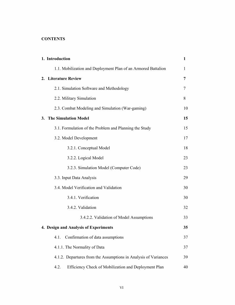
CONTENTS
1. Introduction 1
1.1. Mobilization and Deployment Plan of an Armored Battalion 1
2. Literature Review 7
2.1. Simulation Software and Methodology 7
2.2. Military Simulation 8
2.3. Combat Modeling and Simulation (War-gaming) 10
3. The Simulation Model 15
3.1. Formulation of the Problem and Planning the Study 15
3.2. Model Development 17
3.2.1. Conceptual Model 18
3.2.2. Logical Model 23
3.2.3. Simulation Model (Computer Code) 23
3.3. Input Data Analysis 29
3.4. Model Verification and Validation 30
3.4.1. Verification 30
3.4.2. Validation 32
3.4.2.2. Validation of Model Assumptions 33
4. Design and Analysis of Experiments 35
4.1. Confirmation of data assumptions 37
4.1.1. The Normality of Data 37
4.1.2. Departures from the Assumptions in Analysis of Variances 39
4.2. Efficiency Check of Mobilization and Deployment Plan 40

VII
4.2.1. Test whether the Mobilization and Deployment Plan Meets
The Time Specifications 41
4.2.2. Bottleneck Analysis 42
4.3. 25 Factorial Design for Maximum Time in System Measure 43
4.3.1 Interpretation of Main Effects and Interactions 44
4.4. 25 Factorial Design for Number of Damaged Vehicles Measure 49
4.4.1. Interpretation of Main Effects 50
4.5. 25 Factorial Design for Number of Totally Destructed Vehicles
Measure 51
4.5.1. Interpretation of Main Effects 52
4.6. Conclusions 53
5. Selecting the Most Critique Region of Turkey 56
5.1. Selecting the Most Critique Region of Turkey Among Ten Regions
According to the Maximum Time in System Measure 58
5.2. Selecting the Most Critique Region of Turkey Among Ten Regions
According to the Average Time in System Measure 59
5.3. Selecting the Most Critique Region of Turkey Among Ten Regions
According to the Number of Damaged Vehicles Measure 61
5.4. Selecting the Most Critique Region of Turkey Among Ten Regions
According to the Number of Totally Destructed Vehicles Measure 62
5.5. The Analytic Hierarchy Process 63
5.6. The Detailed Results of Number of Damaged Vehicles and
Number of Totally Destructed Vehicles Measure 66

VIII
5.7. Conclusions 66
6. Selecting the Most Critical Factor Out of Five for Each Regions of Turkey
According to the Number of Totally Destructed Vehicles Measure 68
6.1 Rankings of Factors for Regions 69
6.2 Conclusions 72
7. Limits of Mobilization and Deployment Plan 73
7.1 Scenario 1 73
7.2. Scenario 2 74
7.3. Conclusions 76
8. Conclusions 78
8.1 General 78
8.2. Design and Analysis of Experiments 79
8.3. Selecting the Most Critical Region of Turkey Out of Ten 81
8.4. Selecting the Most Critical Factor Out of Five for Each Regions of Turkey
According to the Number of Totally Destructed Vehicles Measure 82
8.5. Limits of Mobilization and Deployment Plan 82
8.6. Concluding Remarks 83
8.7. Future Research Topics 83

IX
APPENDIX
A Structure of a Turkish Armored Battalion 85 B Output Data for Chapter 4 86
C Output Data For Chapter 5 97 D Code of the Simulation Model 108 E Probability Tree of The System 110 Bibliography 116

X
LIST OF FIGURES 1.2.1. The march plan of Armored Battalion 4
3.1. Schematic view of model development 18
3.2.2.1. Flow charts of Mobilization and Deployment of Armored Battalion 24
3.4.2. A sight of our simulation model 34
4.1.1.1. Normal probability plot of residuals of maximum time in system
measure 38
4.1.1.2. Normal probability plot of residuals of number of damaged vehicles
Measure 38
4.1.1.3. Normal probability plot of residuals of number of totally destructed vehicles
measure 38
4.1.2.1. Scatter diagram of variances of maximum time in system measure 39
4.1.2.2. Scatter diagram of variances of number of damaged vehicles measure 40
4.1.2.3. Scatter diagram of variances of number of totally destructed vehicles
Measure 40
4.2.2. Sensitivity analysis of repair teams 43
4.3.1.1. Main effect of diagram of five factors for maximum time in
system measure 45
4.3.1.2. Interaction between breakdown of vehicles and air attack of enemy 46
4.3.1.3. Interaction between breakdown of vehicles and minefield of enemy 47
4.3.1.4. Interaction between breakdown of vehicles and ambush of enemy 48
4.3.1.5. Interaction between air attack and ambush of enemy 48
4.4.1.1. Main effect diagram of five factors for number of damaged
vehicles measure 50
4.5.1.1. Main effect diagram of five factors for number of totally destructed vehicles
measure 52

XI
LIST OF TABLES
2.1. Summary table of related literature 14
3.3.1. Readiness and pull-off times of vehicles 31
3.3.2. Repair times of vehicles 31
3.3.3. Hit and kill probabilities of guns used in our model 31
4.1. The factor names and levels 37
4.1.1. Bartlett’s test results for variance homogeneity 39
4.2.1. Results and one-sided confidence intervals for time specifications 41
4.3. Factor names and roles for design points 87
4.3.1. Results, averages and variances of 20 replications for maximum time
in system measure for experimental design 88
4.3.2. Results, averages and variances of 20 replications for maximum time
in system measure for experimental design 88
4.3.3. Results, averages and variances of 20 replications for maximum time
in system measure for experimental design 89
4.3.4. Results, averages and variances of 20 replications for maximum time
in system measure for experimental design 89
4.3.5. Effects and results of Analysis of Variance for maximum time in
system measure 90
4.4.1. Results, averages and variances of 20 replications for number of damaged vehicles
measure for experimental design 91
4.4.2. Results, averages and variances of 20 replications for number of damaged vehicles
measure for experimental design 91
XII
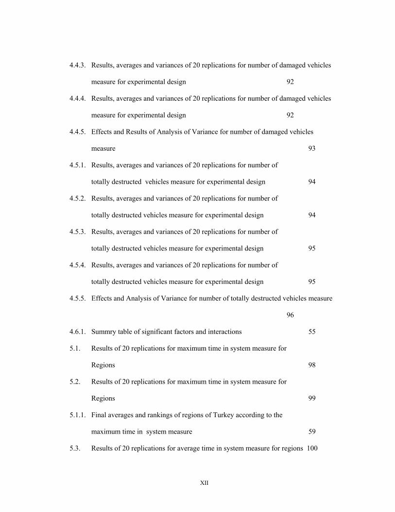
4.4.3. Results, averages and variances of 20 replications for number of damaged vehicles
measure for experimental design 92
4.4.4. Results, averages and variances of 20 replications for number of damaged vehicles
measure for experimental design 92
4.4.5. Effects and Results of Analysis of Variance for number of damaged vehicles
measure 93
4.5.1. Results, averages and variances of 20 replications for number of
totally destructed vehicles measure for experimental design 94
4.5.2. Results, averages and variances of 20 replications for number of
totally destructed vehicles measure for experimental design 94
4.5.3. Results, averages and variances of 20 replications for number of
totally destructed vehicles measure for experimental design 95
4.5.4. Results, averages and variances of 20 replications for number of
totally destructed vehicles measure for experimental design 95
4.5.5. Effects and Analysis of Variance for number of totally destructed vehicles measure
96
4.6.1. Summry table of significant factors and interactions 55
5.1. Results of 20 replications for maximum time in system measure for
Regions 98
5.2. Results of 20 replications for maximum time in system measure for
Regions 99
5.1.1. Final averages and rankings of regions of Turkey according to the
maximum time in system measure 59
5.3. Results of 20 replications for average time in system measure for regions 100

XIII
5.3. Results of 20 replications for average time in system measure for
regions 101
5.2.1. Final averages and rankings of regions of Turkey according to the
average time in system measure 60
5.4. Results of 20 replications for number of damaged vehicles
measure for regions 102
5.5. Results of 20 replications for number of damaged vehicles measure
for regions 103
5.3.1. Final averages and rankings of regions of Turkey according to the number
of damaged vehicles measure 61
5.6. Results of 20 replications for number of totally destructed vehicles
measure for regions 104
5.7. Results of 20 replications for number of totally destructed vehicles
measure for regions 105
5.4.1. Final averages and rankings of regions of Turkey according to the
number of totally destructed vehicles measure 62
5.5.1. Objective matrix of three performance measures for AHP 63
5.5.2. Normalized objective matrix and weights of regions for AHP 64
5.5.3. The results and weights of regions for AHP 65
5.5.4. Final scores of regions via AHP 65
5.6.1. The number of damaged-wheeled trucks by five factors 106
5.6.2. The number of damaged-wheeled trucks by five factors 106
5.6.3. The number of damaged armored vehicles by five factors 106
5.6.4. The number of damaged armored vehicles by five factors 106
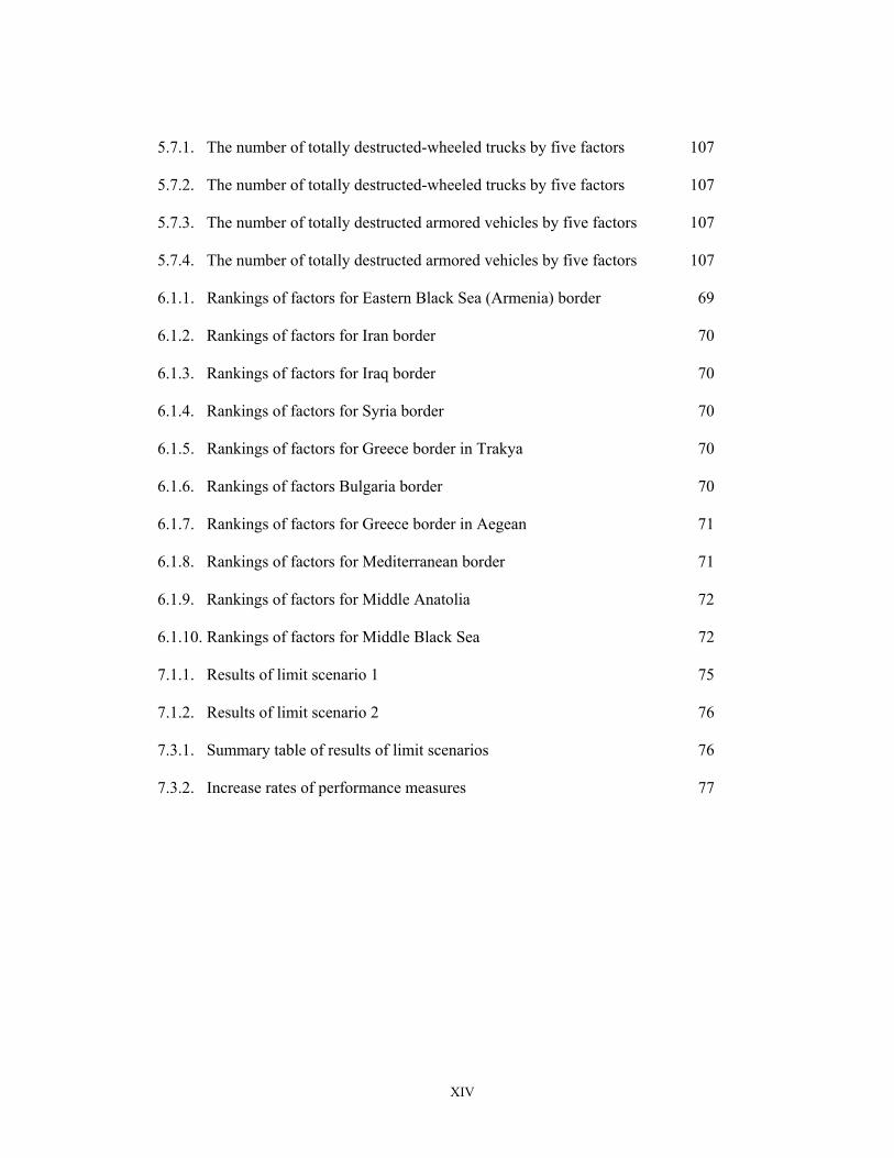
XIV
5.7.1. The number of totally destructed-wheeled trucks by five factors 107
5.7.2. The number of totally destructed-wheeled trucks by five factors 107
5.7.3. The number of totally destructed armored vehicles by five factors 107
5.7.4. The number of totally destructed armored vehicles by five factors 107
6.1.1. Rankings of factors for Eastern Black Sea (Armenia) border 69
6.1.2. Rankings of factors for Iran border 70
6.1.3. Rankings of factors for Iraq border 70
6.1.4. Rankings of factors for Syria border 70
6.1.5. Rankings of factors for Greece border in Trakya 70
6.1.6. Rankings of factors Bulgaria border 70
6.1.7. Rankings of factors for Greece border in Aegean 71
6.1.8. Rankings of factors for Mediterranean border 71
6.1.9. Rankings of factors for Middle Anatolia 72
6.1.10. Rankings of factors for Middle Black Sea 72
7.1.1. Results of limit scenario 1 75
7.1.2. Results of limit scenario 2 76
7.3.1. Summary table of results of limit scenarios 76
7.3.2. Increase rates of performance measures 77

XV
GLOSSARY
AIR ATTACK: Assault with air combat vehicles (warplane, helicopter).
ALERT DISPERSION AREA: Area where the troops spread for minimizing the
casualties during an enemy attack.
ALERT AND MOBILIZATION PLAN: The plan that troops execute for
being ready for combat as soon as possible.
AMBUSH: An unexpected, trap-type military operation.
ARTILLERY ATTACK: Assault with the artillery guns (cannons).
ASSEMBLY AREA: The area where troops make last preparations for further military
operations.
BREAKDOWN: Malfunctioning of the vehicles.
DEPLOYMENT: The strategic relocation and concentration of forces and their
support base (manpower and logistics) from barrack into a theater.
MARCH: Travelling of troops under the threat of enemy.
MINEFIELD: An area where the ground mines are positioned.
MOBILIZATION: A process by which the armed forces reach a state of enhanced
readiness in preparation for war or other national emergencies.

1
CHAPTER 1
INTRODUCTION
1.1. MOBILIZATION AND DEPLOYMENT PLAN OF AN ARMORED
BATTALION
Mobilization describes a process by which the armed forces reach a state of
enhanced readiness in preparation for war or other national emergencies. It includes
activating all or part of the reserve component as well as assembling and organizing
personnel, supplies, and material prior to deployment. Strategic deployment is the
strategic relocation and concentration of forces and their support base (manpower and
logistics) from barrack into a theater. Deployments may take the form of a forcible entry
for crisis response or unopposed entry for natural disasters or humanitarian (Department
of Army, 1996). We do not handle the activities of the reserve components; we deal with
the activities of active components of an Armored Battalion.
We model the mobilization and deployment of an Armor Battalion to Assembly
Area via simulation. The aim of mobilization and deployment is to be ready for combat
with minimum casualties and equipment loss. This activity has to be made as soon as
possible, because it occurs under the disturbance of enemy, any lateness can cause many
human casualties. Because of that reason evaluation of mobilization and deployment
plan has great importance in military.
An armored battalion is formed from four companies. First three companies are
identical armored (tank) companies; the other one is Headquarters and Headquarters
Company. In our simulation model an Armored Company has nine wheeled trucks,

2
fourteen armored vehicles (13 tanks and 1 APC). The Headquarters and Headquarters
Company has twenty-three armored vehicles, seventy-five, wheeled trucks. In total
Armored Battalion have 65 armored vehicles and 102-wheeled trucks.
As a strategy when there is a sense of danger or threat, Turkish Army starts to
load ammunition, gas and equipment to the vehicles for being totally ready for future
operations. So when the alert order is announced, most of equipment and ammunition
has already been loaded. Troops only make partial loading after alert order.
Mobilization starts with the alert order, immediately soldiers start to make partial
loading of equipment and guns quickly. Without waiting others, each vehicle starts to
travel from garages to Alert Dispersion Area individually to minimize the casualties and
vehicle losses caused by enemy attacks. The breakdown of vehicles may occur in garage
after alert order, the other vehicles pull off the broken vehicles to the Alert Dispersion
Area. In daytime at most in half an hour, at night in 45 minutes from the alert order,
Armored battalion has to complete its deployment to Alert Spread Area. After an hour
from the alert order, reconnaissance group starts to travel Assembly Area to secure the
roads and Assembly Area from enemy. Approximately after two hours from the alert
order, main troops have to be ready for travelling to Assembly Area.
In Alert Dispersion Area, Armored Battalion members make preparations for
travelling to Assembly Area that is the last place to complete the preparations for
combat. During travel, vehicle breakdowns can occur, enemy can make air and artillery
assaults, lay ambush and use ground mines to destruct vehicles and kill soldiers. These
assaults of enemy cause vehicle destruction and delay that will affect the success of
further operations. When a vehicle is shot, its crew moves off the vehicle out of road not
to prevent traffic and tries to repair. If the damage is not repairable for the crew, they

3
wait for the maintenance team. Maintenance team arriving shot area immediately begins
to repair the vehicle. If vehicle is destructed completely, it is left in a safe region with its
crew, and maintenance team continues travelling. In our study, activity ends when the
troops reach Assembly Area. We do not deal with the activities in Assembly Area. The
figure 1.2.1. shows the travel plan of Armored Battalion.
We study on the system that starts with the alert order, and ends with the arriving
of all vehicles to Assembly Area. We do not cope with the activities before the alert
order, and we assume that before the alert order, ammunition and fuel oil loadings are
completed, and most of the equipment is loaded to wheeled-trucks. We analyze the
system in the name of vehicles; we do not deal with the soldiers individually.
In this study, we evaluate the performance of existing Mobilization and
Deployment Plan of a Turkish Armored Battalion. The objectives of this study are to
examine the behavior of existing Mobilization and Deployment Plan of an Armored
Battalion in Turkish Army, establish the nature of relationship among one or more
significant factor and the system performance, analyze the efficiency of this plan,
compare different scenarios and improve system performance. We also try to detect the
most hazardous border of Turkey and the most hazardous factor for each border, and
discover the system limits. We focus on five factors that are breakdowns of vehicles, air
attack, artillery attack, mine fields and ambushes of enemy in our study.
We give a brief summary of usages below. In the situation of the system does not
work properly, we try to detect the major problem areas (bottlenecks) of the system by
sensitivity analysis, then propose the modifications to make the system work properly.
Determining the significant effects of five factors that we state above can be useful
information for development of the national defense plans.

4
GARAGES Wheeled truck path Armored vehicle path Figure 1.2.1. The march plan of Armored Battalion for wheeled trucks and armored vehicles
Armored Company 1 Headquarters and
Headquarter Company
Armored Company 2
Armored Company 3 depot
depot depot depot
ALERT DISPERSION AREA
Armored Company 1
Armored Company 2
Armored Company 3
Armored Company 3
ASSEMBLY AREA ARMORED BATTALION

5
The defense arrangements may focus on the most significant factors. The most critique
border information may also be used for improvement of the national defense plans.
Selection of the most hazardous factor and rankings of five factors according to the
threat for each border of Turkey may guide the commanders of these armored battalions
for deciding which factors they should emphasize on during the planning of the field
exercises. Being aware of his Armored Battalion’s limits, commanders can make more
healthy decisions that may have chanced the faith of the war.
Chapter organization is as follows. Chapter 2 presents the related literature with
the simulation software and methods; the requirements of military simulation modeling;
combat modeling and simulation applications that provide useful information for
modeling combat activities. Chapter 3 interprets the implementation of simulation model
of Mobilization and Deployment Plan of a Turkish Armored Battalion. Chapter 4
presents experimental design of five factors that breakdown of vehicles, air attack,
artillery attack, minefields and ambushes of enemy. We implement the ANOVA
procedure to find out the significant factors for three different performance measures in
this chapter. Chapter 5 includes the ranking and selection of the most critique region of

6
Turkey out of ten for three different performance measures and we also apply analytic
hierarchy process to identify a mutual most critique region for all of three performance
measures. Chapter 6 interprets the ranking and selection of the most critique factor out of
five factors for each of ten regions in Turkey. Chapter 7 presents the limits of an
Armored Battalion executing the Mobilization and Deployment Plan. In Chapter 8, we
give the conclusions of the research. As a final step, ideas and suggestions for future
researches are listed. In Appendices, outputs and some figures of armored battalion are
given.

7
CHAPTER 2
LITERATURE REVIEW
During the literature review, we have not come across any study that is directly
related with our topic. We meet some of abstracts of military researches conducted in
U.S. but because of privacy of topic, they are not open to publication. So we cannot get
detailed information about these military researches. Instead, we present the references in
three groups that are the simulation software and methodology, military simulation, and
combat simulation (war gaming). As a final step, we give the summary table of related
literature in Table 2.1.
2.1. SIMULATION SOFTWARE AND METHODOLOGY
We construct the frame of our simulation model, verify and validate it under the
light of some of techniques and ideas presented in the papers in this part of literature
review.
Throughout our study we use the basic principles, which stated in Banks (1998).
In this study, the author explains the fundamentals of the modeling methodologies, gives
brief information about the use of simulation and then recommends a stepwise logic for
all phases of simulation. In our thesis, we use ARENA software for coding system
because it is a powerful tool that meets all of our requirements. Takus and Profozich
(1997) explain the software and its capabilities in their tutorial.
Sergeant (1998) discusses approaches to verification and validation of simulation
models and how model verification and validation relate to the model development

8
process. After defining various validation techniques he describes conceptual model
validity, model verification, operational validity, and data validity and recommends a
procedure.
Kleijnen (1999) explains which statistical techniques can be used to validate
simulation models depending on which real-life data are available. He categorizes the
situations as the cases of having no data, only output data, both input and output data. To
explain these three cases he provides some case study summary.
Alexopoulos and Seila (1998), Kelton (1997), Centeno and Reyes (1998), and
Sanchez (1998) all study on the procedures, techniques about the simulation output
analysis. We use the techniques determined for the terminating systems.
2.2. MILITARY SIMULATION
The papers in that section discuss the general military issues and necessary
techniques for military modeling and simulation. By the help of this literature, we
understand the military aspect of simulation and recognize the differences of military
simulation. We take the guidance of these papers for overcoming of the problems that
we encounter during the model development (lacking of real data, etc.). We also
implement techniques for verification, validation and accreditation of military models
mentioned in some of these papers.
Page and Smith (1998) give the overview of military training simulation in the
form of an introductory tutorial. They provide basic terminology, and current trends and
research focus in the military simulation domain. Also they explain verification,
validation and accreditation of military models.
The Department of Defense (DoD) is currently embracing object-oriented

9
programming as a possible solution to problems that beset current simulation tools in the
paper of Painter (1995). He mentions about the benefits that are object reuse (sharing
objects between simulations), data hiding (encapsulation), and code reuse and extension
(polymorphism) and also the associated cost as a paradigm. Finally he states that the
immediate need facing the military simulation is to agree on and build a framework for
object-oriented simulations.
Smith (1998) identifies and explains essential techniques necessary for modern
military training simulations. He provides a brief historical introduction; discussion of
system architecture; multiple interactive training simulations; event and time
management; distributed simulation; and verification, validation, and accreditation. After
all, he discusses the fundamental principles in modeling and specific military modeling
domains. While discussing the fundamental principles of modeling, he stresses on the
importance of modeling the right problem, complete and accurate understanding,
credibility and construction of the model subject to some constraints. Under the heading
of physical modeling, he focuses on the importance and usage of physical objects, which
include vehicles, people, and machinery involved in the activities of moving, perceiving
other objects, and interacting with them in the military simulations. Behavioral,
environmental and multi-resolution modelings are the other discussed subjects in his
study.
Kang and Roland (1998) discuss the military simulation within the subjects of
organizations that deal with and their areas of study, classification of military simulation,
simulation as a training tool, and applications. They stress on the subjects of advanced
distributed simulation, distributed interactive simulation, and high-level architecture.
Roland (1998) gives an overview of the panel “The future of military simulation”

10
in which military simulation is categorized as including engineering models, analyses
models and training models. The members answer the questions about their background;
goals and objectives of their involvement in modeling and simulation; HLA studies;
major problems in the current state of modeling and simulation development and use;
today’s major modeling and simulation opportunities and challenges.
Sisti (1996) studies on the topics of interest to researchers in the simulation
community and present some of selected Air Force programs. He deals with the wide
variety of research issues in simulation science being presented by government,
academia and industry, and their application to the military domain.
Hatley (1997) discusses the difficulties, ways and cost of the military simulation
model validation and verification. He compares the other simulation models with the
military ones in terms of validation, verification and accreditation.
Kathman (1995) summarizes the data collection process in field combat
simulation of U.S. Army. He describes four basic types of instrumentation that have been
developed to assist data collection in field combat simulation and gives explanations of
these four basic types.
2.3. COMBAT MODELING AND SIMULATION (WAR-GAMING)
Our simulation model is an example of combat simulation because it includes the
combat activities (air attack, artillery assault, mine fields and ambushes of enemy). We
give the some of the applications of war-gaming in that section. To reach detailed
information about war-gaming applications is nearly impossible because they are kept as
secret projects. Under the light of limited information, we implement some of war-
gaming modeling techniques used in these combat simulation applications for some parts
11
of our model during the model development.
Caldwell, Wood and Pate (1995) summarize a two-year project, called JLINK,
which enables the JANUS, Army constructive interactive simulation to be connected to
manned land and air combat vehicle simulators, using Distributed Interactive Simulation
(DIS) Protocol Data Units (PDU). The JLINK project was one of the firsts to
demonstrate that a constructive simulation can be connected to and realistically interact
with DIS compliant virtual combat vehicle and aircraft simulators. They discuss how this
was accomplished, highlight the major considerations involved, and describe the
interface model that was developed to connect JANUS to the DIS world.
Parker (1995) explains a unique approach developed for analyzing force
structures of the armed forces of U.S. With this approach, new ways of measuring
combat readiness are available to ensure that the armed forces remain ready to fight
during the defense draw down of the 1990s. He explains a network representative
language Dynamic Simulation that combines the continuous variable features of system
dynamics and the discrete event features of conventional simulation techniques.
Mostaglio, Johnson and Peterson (1993) give an overview of a Distributed
Interactive Simulations (DIS) training system used by Army, which is called The Close
Combat Tactical Trainer (CCTT). They discuss how it will use the DIS standard
protocols and semi-automated forces within its architecture, the program’s development
methodology, and its role in future Army training.
Childs and Lubaczewski (1987) propose a simulation model used for training
Brigade and Battalion commanders and their staffs to exercise procedures and decision-
making skills. They briefly address the background of command and control training and
provide an in-depth discussion of the COMBAT-SIM model.
12
Parker (1991) gives an overview of combat vehicle reliability assessment
simulation model, which portrays the disposition, or status of vehicles over time. He also
suggests using this information to initialize the other combat models in which reliability
may not previously have been a consideration.
Allen and Wilson (1988) describe a methodology for developing combat
simulations that may be readily tailored to specific study issues, and structured so as to
threat both qualitative and quantitative variables using the natural language of military
planners. This methodology was developed for the RAND Strategy Assessment System
(RSAS) and exploits a new programming language called RAND-ABEL. They also
explain in what areas RAND-ABEL language is used.
Blais (1994) gives the description of a computer assisted, two-sided warfare
gaming system designed to support training of U.S. Marine Corps commanders and their
staffs. He explains development phases and usage areas of this simulation system, which
is called The Marine Air Ground Task Force Tactical Warfare Simulation.
Henry (1994) describes The Corps Battle Simulation as a standard tool for
training commanders and their staffs in U.S. Army. This simulation model is written in C
programming language, and combat is modeled mathematically using Lanchester-type
equations as described by Taylor (1981). He also stated the hardware and evolution of
The Corps Battle Simulation.
Youngren, Parry, Gaver and Jacobs (1994) give description of a research
conducted at the Naval Postgraduate School into new methodologies for joint theater-
level combat simulation modeling, emphasizing C31, operational intelligence, decision
making under certainty, and aggregated stochastic process modeling. Research outcomes
to date as well as a prototype software tool are described in their paper.

13
Russell and McQuay (1993) give an overview of a system called The Joint
Modeling and Simulation System (J-MASS) whose development standards and software
tools support a disciplined approach to the development, configuration, operation, and
analysis of digital models and simulations. They explain that J-MASS provides a
common modeling architecture with a library of verified and validated software
components and models of weapon systems developed by different military communities
for Department of Defense. Oswalt (1995) presents the technologies critical to military
simulation, summarizes their status, proposes a concept of what technologies are likely
to be applied in the future military simulations, and concludes with a review of two
current simulation architectures-SIMOBJECT and J-MASS.
Garrambone (1992) gives an overview of one of the most difficult topics of
Operations Research- combat modeling and simulation. He describes a team leader
standpoint, the requirements, which drive the modeling process used to support DoD
studies. He discusses models, (sources and construction notes), scenarios, data, computer
concepts, team composition, and many other important considerations needed to
accomplish the analytical study tasks. The reader, novice or seasoned, will find that this
approach to the subject contains insights rarely found in manuals, covering topics from
defining the study environment, to the techniques for presenting study results.
Garrabrants (1998) proposes “an expansion of simulation systems’ role to support
all levels of command and control functioning, especially staff planning after receipt of
orders and mission rehearsal” in this study. He explains how Marine Tactical Warfare
Simulation (MTWS), an advanced simulation system, is used to model all aspects of
combat (air, land, sea, and amphibious ship-to-shore activities) and gives detailed
information about its usage. We give summary of related literature in Table 2.1.

14
Table 2.1. Summary table of related literature
Simulation Software and Methodology
Takush and Profozich (1997) Sargent(1998) Sanchez (1998) Kleijnen (1999) Alexopoulos & Seila (1998) Centeno & Reyes (1998) Kelton (1997)
ARENA software tutorial Verification and validation of simulation models ABC’ s of output analysis Statistical techniques and data availability Advanced methods for simulation output analysis Simulation output analysis Statistical analysis of simulation output
Military Simulation
Page & Smith (1998) Painter (1995) Smith (1998) Kang & Roland (1998) Roland (1998) Sisti (1996) Hatley (1997)
Introduction to military training simulation Object oriented military simulation development and application Essential techniques for military modeling and simulation Military simulation The future of military simulation Modeling and simulation technologies for military applications Verification and validation in military simulation
Combat Modeling and Simulation
Caldwell & Wood & Pate (1995) Parker (1995) Mostaglio, et al. (1993) Childs & Lubaczewski (1987) Parker (1991) Allen & Wilson (1988) Blais (1994) Henry (1994) Youngren, et al. (1994) Russel & McQuay (1993) Kathman (1995) Garrambone (1992) Garrabrants (1998)
JLINK-JANUS fast movers Military force structure and realignment “ sharpening the edge” through the dynamic simulation The close combat tactical training program A battalion / brigade training simulation Combat vehicle reliability assessment simulation model Modeling qualitative issues in military simulations with the RAND-ABEL language. Marine air ground task force tactical warfare simulation The corps battle simulation The future theater-level model The joint modeling and simulation Data collection in field combat simulation An overview of air land combat modeling and simulation Simulation as a mission planning

15
CHAPTER3
THE SIMULATION MODEL
3.1. FORMULATION OF THE PROBLEM AND PLANNING THE STUDY
The objectives of this study are to examine the behavior of existing Mobilization and
Deployment Plan of an Armored Battalion in Turkish Army, establish the nature of
relationship among significant factors and the system performance, analyze the
efficiency of Mobilization and Deployment plan of an Armored Battalion, compare
different scenarios and improve system performance. In the case where the system does
not work properly, we try to detect the major problem areas of the system, and then
propose the modifications to make the system work properly. Specifically, we will
attempt to answer the following research questions:
• Is the existing plan efficient?
• After alert order, can whole battalion reach to Alert Dispersion Area in 30
minutes in daytime, 45 minutes at night?
• After alert order, can reconnaissance force at most in one hour, main force in two
hours be ready for moving to the Assembly Area?
• Where does the bottleneck occur in the system?
• How does air attack, artillery assault, mine fields and ambush of enemy affect the
system performance?
• Which region of Turkey is most vulnerable against enemy attack?
• Which factor(breakdown of vehicles, air attack, artillery assault, mine fields and
ambush of enemy ) is the most hazardous for each region of Turkey?

16
• What are the limits of an Armored Battalion executing Mobilization and
Deployment Plan?
• Can I suggest a better alternative plan?
The performance measures under consideration are:
• Average time in system measure of last vehicle reaching the assembly area
• Average time in system measure of vehicles
• Number of damaged vehicles
• Number of totally destructed vehicles
Since the mobilization and deployment are a part of combat, the data requirements
are hard to provide. The data requirements of our simulation model are:
• Loading time data
• Velocities of tanks and wheeled trucks
• Repairing time distributions of damaged vehicles by breakdowns, air attack,
artillery attack, mine and ambush
This study helps to see how the Mobilization and Deployment Plan works, how the
behavior of system changes under the certain conditions and different scenarios. The end
user of this study is Armored Battalion Commanders of Turkish Army. We model the
system by using the following assumptions:
• Armored Battalion in our model is an independent mission battalion
• Basic unit is company
• The construction of Armored Battalion is in Appendix and it is taken from the
Turkish Military Logistics Procedure (1994).
• Velocity of armored vehicles are 29 km/h

17
• Velocity of wheeled trucks are 40 km/h
• Ambush guns are 4 LAWs
• Artillery guns are 4 155mm. Cannons
• Air attack gun is 1 F-16 war plane
• Mine density on the path of vehicles is 6 anti-tank mines in a 8*8 mine field
3.2. MODEL DEVELOPMENT
First, we start with the forming the conceptual model to develop our simulation
model. During this phase, we consult the Armored Battalion, Armored Company and
Team commanders who are the main actors of Mobilization and Deployment Plan. We
also interview with the staff officers who are the experts of planning of military
operations to build the logical model. Then we write the code of model by using ARENA
software. Figure 3.1 gives the schematic view of model development.
Figure 3.1.Schematic view of model development
3.2.1. CONCEPTUAL MODEL
We form a conceptual model of Mobilization and Deployment Plan of Armored
Brigade to convert the real system into a simple system to examine the structure and
components, which should be included. The Mobilization and Deployment Plan is
REAL WORD SYSTEM
ASSUMED SYSTEM
CONCEPTUAL MODEL
LOGICAL MODEL
SIMULATION MODEL

18
used by all troops in Turkish Army. The frame of plan is the same for all kinds of troops
(armored, artillery, infantry etc.). Only minor differences are made to plan according to
the positioning and structure of troop, mission type etc. During conceptualization, we
interview with armored battalion, company, team commanders and staff officers. The
basic elements of the simulation model is given below:
Events:
Events are instantaneous occurrences that change the state of the system. The lists of
events that occur in our simulation model are:
• Announcement of alert order event: The alert order is given to battalion by the
intelligence service. Soldiers take their personal equipments and guns, and then make
partial loading of equipment to the wheeled trucks.
• Departure of vehicles from garages event: After the completion of loading and
preparation, vehicles start to travel to Alert Dispersion Area independent of others.
• Arrival of vehicles to Alert Dispersion Area event.
• Departure of reconnaissance force from Alert Dispersion Area event: The
reconnaissance force starts to travel to Assembly Area for securing the roads and
Assembly Area.
• Breakdown of vehicles during march from Alert Dispersion Area to Assembly Area
event: The broken vehicle is moved off the road not to prevent traffic flow and wait
for repairing by maintenance team.
• Air attack of enemy during march event: The damaged vehicle is moved off the road
not to prevent traffic flow and wait for repairing by maintenance team. If the vehicle
is totally destructed, it is left in a safe area. The same procedure is also valid for in
the situation of artillery assault, ambush and mine fields.

19
• Artillery assault of enemy during march event.
• Hitting ground mines of enemy during march event.
• Ambush of enemy event.
• Failure of vehicles because of air and artillery attack, breakdowns, ground mines and
ambushes.
• Completion of repair of damaged and broken vehicles event.
• Departure of damaged and broken vehicles from the repair areas event.
• Arrival of totally destructed vehicles to a safe area.
• Arrival of vehicles to Assembly Area event.
Entities:
Entities are the objects of an interest in the system that requires an explicit
representation in the system. There is only one type of entity in our system and it is
vehicles of Armored Battalion.
Attributes:
Attributes are the characteristics of the entities. In our model, we have the
following attributes:
• The beginning time of Mobilization activity
• Company identification numbers
• Vehicle identification numbers
• Type of damage that the vehicle takes
• Air attack identification numbers (helicopter or plane attack)
Activities:
Activity represents a time period of specified length. Some of activities are:

20
• Equipment loading in garages
• March of vehicles from garages to Alert Dispersion Area
• Preparation of main troops of Armored Battalion in Alert Dispersion Area for march
to Assembly Area
• March of Armored Battalion from Alert Dispersion Area to Assembly Area
Exogenous Variables (Input Variables):
We have two types of input variables: decision variables(controllable variables)
and parameters(uncontrollable variables).
Decision Variables:
• Velocity of vehicles
Parameters
• Time that we spent for partial loading of equipment and preparation for march to
Alert Dispersion Area (most of the equipment (ammunition, guns etc.) is loaded
before the alarm order according to the intelligence report, only the equipment that is
essential for soldiers to continue their daily activities in barracks is left unloaded.)
• Readiness time of reconnaissance force for march to Assembly Area from Alert
Dispersion Area
• Readiness time of main force (Armored Battalion) for march to Assembly Area from
Alert Dispersion Area
• Repair time of vehicles broken by breakdowns
• Repair time of vehicles damaged by air attack, artillery assault, mine fields and
ambushes

21
Endogenous Variables (Output Variables):
We classify the endogenous variables as state variables and performance
measures.
State Variables:
• Number of vehicles waiting in the repair queues
• Number of vehicles that does not damaged or broken in the convoy
• State of repair units (busy or idle)
Performance Measures
• Average time in system measure of last vehicle reaching the assembly area
• Average time in system measure of vehicles
• Number of damaged wheeled trucks because of breakdowns
• Number of damaged wheeled trucks because of air attack
• Number of damaged wheeled trucks because of artillery assault
• Number of damaged wheeled trucks because of ground mines
• Number of damaged wheeled trucks because of ambush
• Number of damaged armored vehicles because of breakdowns
• Number of damaged armored vehicles because of air attack
• Number of damaged armored vehicles because of artillery assault
• Number of damaged armored vehicles because of ground mines
• Number of damaged armored vehicles because of ambush
• Number of totally destructed wheeled trucks because of breakdowns
• Number of totally destructed wheeled trucks because of air attack
• Number of totally destructed wheeled trucks because of artillery assault

22
• Number of totally destructed wheeled trucks because of ground mines
• Number of totally destructed wheeled trucks because of ambush
• Number of totally destructed armored vehicles because of breakdowns
• Number of totally destructed armored vehicles because of air attack
• Number of totally destructed armored vehicles because of artillery assault
• Number of totally destructed armored vehicles because of ground mines
• Number of totally destructed armored vehicles because of ambush
• Total number of damaged vehicles
• Total number of totally destructed vehicles
3.2.2 LOGICAL MODEL
Logical model shows the relationships among the elements of the model. We
construct the logical model of Mobilization and Deployment Plan of a Turkish
Armored Battalion. Our model starts with the receiving of alert order and ends with
the occupation of Assembly Area by the Armored Battalion. The main events that
our model includes are the partial loading of the wheeled-trucks, march of Armored
Battalion from garages to Alert Dispersion Area, march from Alert Dispersion Area
to Assembly Area, and attacks of enemy against the Armored Battalion during this
march. During the construction of logical model, we take the consultancy of
Armored Battalion and Company commanders who are the executers of the
Mobilization and Deployment Plan. We present the relationship among the elements
of the Mobilization and Deployment Plan of an Armored Battalion in Figure 3.2. as
flow charts.

23
Figure 3.2. Flow chart of Mobilization and Deployment of Armored Battalion
Alarm order is given
Soldiers take their personal equipment and run to garages
Partial loading of equipment is done
One wheeled truck is immediately be ready for travel headquarters building for command equipment
Does breakdown occur?
YES
NO
Repair
Start to travel headquarters building
Ready for traveling to Alert Dispersion Area
Does breakdown occur?
YES Repair
NO
Load equipment
Start to travel Alert Dispersion Area
Take the position in Alert Dispersion Area
1

24
Figure 3.2. Flow chart of Mobilization and Deployment of Armored Battalion (con’t)
Preparations for march (military travel) to Assembly Area
Reconnaissance team starts totravel to Assembly Area Armored Battalion
commander gives the march order to main units of battalion
Main units continue preparation for march
Start march to Assembly Area
Does usual breakdown occur during march?
NO
YES Repairable?
NO
Leave the destructed vehicle in a safe zone with its crew.
YES
Repair
Continue to march (travel)
2
1

25
Figure 3.2. Flow chart of Mobilization and Deployment of Armored Battalion (con’t)
2
Air attack of enemy occurs
Move off all vehicles from road for minimize casualty
Wait at least 60 seconds forair attack to pass
Is vehicle shot? YES Repairable? NO
Leave the vehicle in a safe place with its crew.
YES
Repair
NO
Continue to march
Artillery assault occurs
3

26
Figure 3.2. Flow chart of Mobilization and Deployment of Armored Battalion (con’t)
Is the vehicle shot?
YES Repairable?
NO
Leave the vehicle in a safe zone with its crew.
YES
NO
Repair
Go on march to Assembly Area
Minefield of enemy exists.
Is vehicle hit the mine?
YES
NO
Clear the minefield
Repairable? NO
Leave the vehicle with its crew.
YES
Repair
Continue march to Assembly Area
4
3

27
Figure 3.2. Flow chart of Mobilization and Deployment of Armored Battalion (con’t)
4
Ambush of enemy occurs.
Is vehicle shot? YES Repairable? NO
Leave the vehicle in a safe area with its crew.
NO
YES
Repair
Continue march to Assembly Area
Occupy the Assembly Area

28
3.2.3 SIMULATION MODEL (COMPUTER CODE)
Although our simulation model can be described as a combat simulation, we use
ARENA software, which is not a combat simulation package. Because we need a
detailed evaluation of Mobilization and Deployment Plan. The Mobilization and
Deployment Plan include the activities just before the war. In other words, it organizes
the combat preparation and alert activities. It is a detailed plan, and every detail is too
important because the objective of plan is to prepare the troops for combat as soon as
possible after alert. As time so important, to model the details is also important. The
currently available combat simulation packages in Turkish Army do not support such
kind of detailed modeling. The most available combat simulation package in Turkish
Army for our subject is JANUS. But it is especially used for modeling the combat area
activities. The Alert, Mobilization and Deployment Plan organizes the combat
preparation and alert activities, not the combat. The details that JANUS cannot model are
stated below:
1) The preparation period which soldiers take their equipment and guns.
2) Loading of equipment to the lorries.
3) The details of modeling the transportation of soldiers and equipment with vehicles.
These activities cannot be modeled with JANUS. Thus, we use ARENA software
for modeling The Alert, Mobilization and Deployment Plan of an Armored Battalion in
Turkish Army. ARENA software is a flexible and powerful tool that allows modeling all
the activities of mobilization and deployment plan of Armored Battalions. It also
provides creating animated models and offers reasonably good simulation input and
output process. We have only one animated model. The computer codes of model occupy
4.68 MB. We give a small part of the code of our simulation model in Appendix D.

29
3.3 INPUT DATA ANALYSIS
As our simulation model is a combat simulation model, we face with lackg of real
data problem. To overcome this problem, we use triangular distributions as
recommended by Banks (1998). We interview with the armored battalion, armored
company and the armored team commanders who are the real executers of Mobilization
and Deployment Plan to determine the triangular distributions of activities. We also take
some of data from the Army Field Manuals that are written according to the combat
experiences. We convert these types of raw data into the triangular distributions via
consulting the experts. We take hit and kill probabilities of guns, and vulnerability of
combat vehicles from the databases of JANUS software. We give the lists of random
variables of our simulation model, distribution functions, and their parameters in Table
3.3.1.-Table 3.3.3.
3.4. MODEL VERIFICATION AND VALIDATION
We perform the Verification and Validation (V&V) techniques stated in the
Army Pamphlet 5-11 published by Department of Army (1999) and Balci (1998) for all
steps of our simulation model.
3.4.1. VERIFICATION
“ Verification of a M&S is the process of determining that an M&S accurately
represents the developer’s conceptual description and specifications” (Army Pamphlet 5-
11, 1999). We applied some of techniques that are stated in Army Pamphlet 5-11 (1999)
for verification of our model.

30
Table 3.3.1. Readiness and pull-off times of vehicles
readiness time after alert order pull of time of broken vehicle in garage wheeled-truck tria (8,10,12) tria (8,12,16) armored vehicles tria (10,12,16) tria (13,15,17)
Table 3.3.2. Repair times of vehicles
type of damage 1 2 3
wheeled trucks breakdown tria(15,20,25) tria(30,35,40) tria(45,50,55) air attack tria(35,40,45) tria(40,45,50) tria(55,60,65) artillery tria(25,30,35) tria(40,45,50) tria(55,60,65)
minefields tria(25,30,35) tria(45,60,75) tria(70,80,90) ambush tria(25,30,35) tria(40,45,50) tria(55,60,65)
armored vehicles breakdown tria(15,20,25) tria(30,35,40) tria(45,50,55) air attack tria(25,30,35) tria(40,45,50) tria(55,60,65) artillery tria(25,30,35) tria(40,45,50) tria(55,60,65)
minefields tria(25,30,35) tria(45,60,75) tria(70,80,90) ambush tria(25,30,35) tria(40,45,50) tria(55,60,65)
Table 3.3.3. Hit and kill probabilities of guns used in our model
for wheeled trucks for armored vehicles hit kill hit kill 30 mm cannon (F-16) 0.1 0.65 0.1 0.55 155 mm cannon 0.08 0.5 0.12 0.35 anti-tank mine 0.02 0.72 0.04 0.27 LAW (ambush gun) 0.04 0.8 0.06 0.55
As logical verification:
• Design Walk-Through: We perform design walk-trough with the Armored
Battalion and Company commanders who are the execution experts of
Mobilization and Deployment Plan to verify the design of our model.
As code verification:
• Sensitivity Analysis: We apply sensitivity analyses to check the algorithms and
code to ensure that our model is reacting in expected manner.

31
• Code Walk-Through: We put into practice code walk-through with the
simulation men from our department to ensure the efficiency, correctness,
consistency and completeness in the implementation.
• Automated Test Tool: We use ARENA debugger function as an automated test
tool to check whether the activities in Mobilization and Deployment Plan occur
properly or not.
• Unit Checks: We also put into use unit checks to ensure that the proper units of
measure results from equations used in algorithms and code of our model (km/h
etc.).
• Additional Statistics: We also check the properness of system performance by
using additional output statistics that are verifying our performance measures
(total time in system etc.).
3.4.2 VALIDATION
“Validation is the rigorous and structured process of determining the extent to

32
which an M&S accurately represents the intended real world phenomena from the
perspective of the intended use of M&S” (Army Pamphlet 5-11, 1999).
As procedural approaches:
• Peer Review: We realize peer reviews, which are the detailed examination of
input data, key parameters and resulting output with the personnel who are
knowledgeable about modeling the functional areas represented in our model. For
this method, we take the consultancy of the military personnel from I.E.
department.
• Independent Review: We implement review with the people independent of our
model development for validation of our model.
As technical methods:
• Face Validation: We put into service face validation to check if our model
seems reasonable to personnel who are knowledgeable about the Mobilization
and Deployment Plan of Armored Battalion. For this purpose, we take the

33
consultancy of Armored Battalion and Company commanders that are the
executers of plan, staff officers that are the experts of military operation
planning. With little modifications towards their comments, we get reasonable
and satisfactorily result.
• Animation: We check the behavior of our system through time by the
animation, especially the movements of vehicles of Armored Battalion. We give
a sight from our simulation model in Figure 3.4.2.

34
Figure 3.4.2. A sight of our simulation model
3.4.2.2 VALIDATION OF MODEL ASSUMPTIONS
We discussed the structural and data assumptions of our model with two
Armored Battalion and Company commanders and one staff officer from Turkish Armor
School. They find these assumptions reasonable for our objectives. We could not
perform statistical validation of output because we do not have actual combat data to
compare.

35
CHAPTER 4 DESIGN AND ANALYSIS OF EXPERIMENTS
Experiments are carried out by investors in all fields of science either to discover
something about a particular process or to compare the effect of several factors on some
phenomena (Montgomery, 1984). For this part of our study, we look for the answers of
questions:
• After alert order, can whole battalion reach to Alert Dispersion Area in 30
minutes in daytime, 45 minutes at night?
• After alert order, can reconnaissance force at most in one hour, main force in two
hours be ready for moving to the Assembly Area?
• Where does the bottleneck occur in the system?
• Is the existing plan efficient?
• How do air attack, artillery assault, mine fields and ambush of enemy affect the
system performance?
We run our simulation model and construct one-sided confidence intervals to check
whether the Mobilization and Deployment Plan satisfies the specifications stated in the
first and second questions. After constructing the confidence intervals, we see that the
existing system meets all the necessary measures. We discuss this procedure in detail in
Section 4.2. To answer the fourth and fifth questions, we just run the simulation model
and check whether the Mobilization and Deployment Plan satisfies the specifications.
We encounter bottlenecks in the repair units of Armored Battalion, because of the longer
waiting queues in front of them. By the sensitivity analysis, we find the optimal number
of repair units for the Armored Battalion. We also implement 2k factorial design for five

36
factors which are breakdowns of vehicles, air attack, artillery attack, mine fields and
ambushes of enemy to find out an answer for the last question. The factors and their
levels are presented in Table 4.1. Our aim is to discover the effects and interactions of
these five factors on system response. Our performance measures are maximum time in
system (time in system of last vehicle reaching Assembly Area), number of damaged
vehicles, and number of totally destructed vehicles. As we have five factors, we have 32
design points. To satisfy the normality assumption, we make twenty replications for each
design point. Because the maximum time in system measure is one of our performance
measures, we should take more replications to satisfy normality. We conduct
experiments for each design point with the 20 replications and calculate the effect of
each factor and their interactions with each other. We implement analysis of variance
(ANOVA) to find out which factor or factors have a significant effect on system
performance and by effect diagrams we explain the main effects and interactions of
factors. We also check normality of data by normal probability plots of residuals and the
homogeneity of variances with scatter diagrams and Bartlett’s test, in Section 4.1.1 and
Section 4.1.2 respectively. To ensure the independence, we assign different random
number generator for each random activity in our simulation model.
We give a name to each design point; names and the roles of factors for each design
point are stated in Table 4 in Appendix B. The expressions “run xyz” in result tables
means the replication that the factors x, y and z are at highest levels whereas the others
are at lowest levels. Our performance measures are maximum time in system (time in
system of last vehicle reaching Assembly Area), number of damaged vehicles, and
number of totally destructed vehicles and we have five factors, we implement the
procedure below for each performance measure.

37
Table 4.1. The factor names and levels
Lower level Upper level factor description (occurrence probability) (occurrence probability) 1 breakdown 0.01 0.06 2 air attack 0 1 3 artillery attack 0 1 4 minefield 0 1 5 ambush 0 1
4.1. CONFIRMATION OF DATA ASSUMPTIONS
Throughout this chapter we assume that (1) data is independent, (2) variances are
homogeny, and (3) the usual normality assumptions are satisfied. To reach correct
results, we need to ensure that all the three assumptions hold for our data. For data
independency, we assign different random number generators for each random event. We
check the normality assumption in Section 4.1.1, homogeneity of variances assumption
in Section 4.1.2.
4.1.1 NORMALITY OF DATA
To ensure the normality of data for three performance measures that we use in
experimental design, we compute the residuals and draw the normal probability plots of
residuals. As all the residual plots in Figure 4.1.1.1 - Figure 4.1.1.3 lie reasonably close
to a straight line; we can say that the data of three performance measures are normally
distributed.

38
Normal probability plot of residuals of max time in system
0102030405060708090
100
-15 -10 -5 0 5 10 15 20 25
residuals
norm
al p
roba
bilit
y
Pj*100
Figure 4.1.1.1 Normal probability plot of residuals of maximum time in system
Normal probability plot of residuals of damaged vehicles
0
20
40
60
80
100
-0,6 -0,4 -0,2 0 0,2 0,4 0,6 0,8
residuals
norm
al p
roba
bilit
y
Pj*100
Figure 4.1.1.2 Normal probability plot of residuals of number of damaged vehicles
Normal probability plot of residuals of numberof totally destructed
0
20
40
60
80
100
-0,5 -0,4 -0,3 -0,2 -0,1 0 0,1 0,2 0,3 0,4residuals
norm
al p
roba
bilit
y
Pj*100
Figure 4.1.1.3 Normal probability plot of residuals of number of totally destructed Vehicles

39
4.1.2 DEPARTURES FROM THE ASSUMPTIONS IN ANALYSIS OF
VARIANCES
The assumptions of homogeneity of variances may cause serious problems in
ANOVA test if it does not satisfied. To check the homogeneity of variances, we draw
scatter diagrams of variances of three performance measures. There is no evidence of
correlation of variances in scatter diagrams (Figure 4.1.2.1-4.1.2.3), to be sure the
homogeneity, we also implement Bartlett’s test. Bartlett’s tests give that the variances of
three performance measures are homogeny. The test results are given in Table 4.1.1.
Thus, we can conclude that the homogeneity assumption of variances holds for our data.
Table 4.1.1 Bartlett's test results for variance homogeneity
time in system # of broken vehicles # of totally destructed grand variance 4134.68 12.91 2.12 q 11.71 18.92 14.88 c 1.02 1.02 1.02 Xo*Xo 26.5 42.79 33.65 chi square(0.05, 31) 44.97 44.97 44.97 test result pass pass pass
max time in system variances
0
2000
4000
6000
8000
0 10 20 30 40
varia
nces
Series1
Figure 4.1.2.1 Scatter diagram of variances of maximum time in system measure

40
number of damaged vehicles variances
0
10
20
30
40
0 10 20 30 40
varia
nces
Series1
Figure 4.1.2.2 Scatter diagram of variances of number of damaged vehicles measure
totally destructed vehicle variances
0
2
4
6
8
0 10 20 30 40
varia
nce
var
Figure 4.1.2.3 Scatter diagram of variances of number of totally destructed vehicles
measure
4.2. EFFICIENCY CHECK OF MOBILIZATION AND DEPLOYMENT PLAN
For the efficiency of the Mobilization and Deployment Plan, we check whether
any bottleneck occurs during the execution of the Mobilization and Deployment Plan and
whether the Armored Battalion satisfies the Turkish Army time standards or not. For the
bottleneck checking, we implement sensitivity analysis. For the control of the time
specifications, we construct confidence intervals.
41
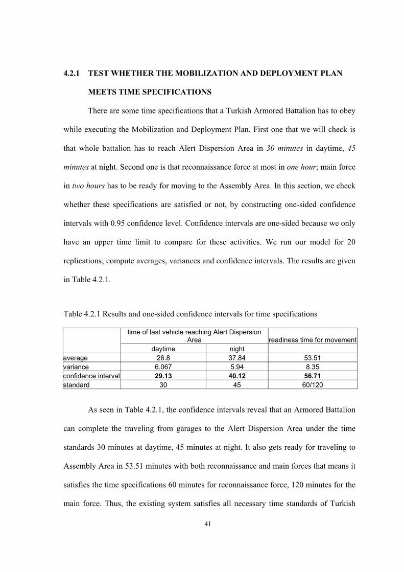
4.2.1 TEST WHETHER THE MOBILIZATION AND DEPLOYMENT PLAN
MEETS TIME SPECIFICATIONS
There are some time specifications that a Turkish Armored Battalion has to obey
while executing the Mobilization and Deployment Plan. First one that we will check is
that whole battalion has to reach Alert Dispersion Area in 30 minutes in daytime, 45
minutes at night. Second one is that reconnaissance force at most in one hour; main force
in two hours has to be ready for moving to the Assembly Area. In this section, we check
whether these specifications are satisfied or not, by constructing one-sided confidence
intervals with 0.95 confidence level. Confidence intervals are one-sided because we only
have an upper time limit to compare for these activities. We run our model for 20
replications; compute averages, variances and confidence intervals. The results are given
in Table 4.2.1.
Table 4.2.1 Results and one-sided confidence intervals for time specifications
time of last vehicle reaching Alert Dispersion Area readiness time for movement
daytime night average 26.8 37.84 53.51 variance 6.067 5.94 8.35 confidence interval 29.13 40.12 56.71 standard 30 45 60/120
As seen in Table 4.2.1, the confidence intervals reveal that an Armored Battalion
can complete the traveling from garages to the Alert Dispersion Area under the time
standards 30 minutes at daytime, 45 minutes at night. It also gets ready for traveling to
Assembly Area in 53.51 minutes with both reconnaissance and main forces that means it
satisfies the time specifications 60 minutes for reconnaissance force, 120 minutes for the
main force. Thus, the existing system satisfies all necessary time standards of Turkish

42
Army.
4.2.2 BOTTLENECK ANALYSIS
During the experiments, we observe that there occur sudden queues in front of
the repair units of breakdown of vehicle, air attack, artillery attack, minefield and
ambush. In our model, we assume that the armored battalion has 5 repair units. We
conduct sensitivity analysis by changing the number of repair units to find out the
optimum number of repair unit for the armored battalion. We conduct these experiments
when all the occurrence probabilities of five factors are 1 (worst case), and observe that
the last vehicle arrives the Assembly Area in 361 minutes when there are 5 repair units.
As a result of sensitivity analysis, we see that the maximum time in system statistic does
not change for the 14 and more repair units. Then we can conclude that 14 repair units
are the optimal quantity for the Armored Battalion. For14 repair units, the maximum
time in system statistic is 216 minutes. Increasing the number of repair units from 5 to 14
provides a %40 decrease in maximum time in system statistic. The behavior of the
maximum time in system statistic depending on the number of repair units is given in
Figure 4.2.2.
Thus, as results of Section 4.2.1 and Section 4.2.2, we can conclude that except the
bottleneck in repair units existing Mobilization and Deployment Plan of a Turkish
Armored Battalion is efficient. The bottleneck can be fixed by increasing the number of
repair units 14 for the armored battalion. But this number is computed when the armored
battalion is exposed to worst enemy threat and the highest vehicle breakdown rate which
means enemy makes air attack, artillery attack, position minefield, lay an ambush and
breakdown rate of vehicle is at highest level during the march to Assembly Area.

43
sensitivity analysis of repair teams
150200250300350400450
4 5 6 7 8 9 10 11 12 13 14 15# of repair team
max
in ti
me
in s
yste
m
Figure 4.2.2. Sensitivity analysis of repair teams
4.3 25 FACTORIAL DESIGN FOR MAXIMUM TIME IN SYSTEM MEASURE
Maximum time in system measure is very important for the Turkish Army
because this measure gives us the time that all the parts of battalion except the totally
destructed ones reach the target and be ready for the further military operations.
Because of that reason, we choose maximum time in system measure as one of our
performance measure. We conduct the thirty-two experiments with twenty
replications and give the results of these replications, with their averages and
variances for every design point in Table 4.3.1- Table 4.3.4 in Appendix B. We
compute the effects at every design point according to the procedure in
Montgomery’s book (1984) and give the results in Table 4.3.5 in Appendix B.
To be able to give a statistical explanation, we implement analysis of variances
(ANOVA) procedure. By ANOVA, we can state which factors have a significant
effect on maximum time in measure. During the implementation of ANOVA, we
compute contrasts and variances of design points and use the F- test to find out

44
which factor has significant effect on system response. The analysis of variances is
also summarized in Table 4.3.5 in Appendix B. We have eight main significant
factors and interactions on maximum time in system measure. The main significant
factors are breakdowns of vehicles (65.68 min.), air attack (71.91 min.), minefields
(12.99 min.) and ambushes (17.3 min.) of enemy as factors, and they all have
positive effects. Air attack has the most positive greatest effect on this performance
measure. As seen only artillery attack does not have a significant effect because its
totally destruction rate is very high. Most of the vehicles affected by artillery attack is
totally destructed and does not cause a delay in maximum time in measure because
the totally destructed vehicles are left in a safe place without repair. The significant
interactions are breakdown- air attack (-28.21 min.), breakdown- mine fields (-12.62
min.), breakdown-ambush (-13.2 min.) and air attack-artillery attack (-11.62 min.).
All the significant interactions have negative effects on maximum time in measure.
We explain the significant factors and interactions in Section 4.3.1 via effect
diagrams.
4.3.1 INTERPRETATION OF MAIN EFFECTS AND INTERACTIONS
We analyze these significant main effects and interactions by using effect
diagrams below. We only give the effect diagrams of significant factors and
interactions. We first discuss the effects of main factors. We draw all the significant
main effects on a single figure to compare and also give the minimum and maximum
values of each effect inside the figure. As seen in Figure 4.3.1.1, the dotted lines of
factors breakdowns of vehicles and air attack of enemy have steeper increase than the
lines of other factors, because number of broken vehicles and number of damaged

45
vehicles by air attack in average are 10.15 and 7.35 vehicles at maximum levels of
these two factors respectively. Repairing them takes much time and this causes
maximum time in system measure to increase.
MAIN EFFECTS
250
275
300
325
350
level of factors
max
tim
e in
sys
tem
breakdown 271,928 337,61
air attack 268,596 340,94
mine 298,496 311,05
ambush 296,34 313,2
min max
Figure 4.3.1.1 Main effect diagram of significant factors
Although average number of damaged vehicles by air attack is smaller than the
average number of broken vehicles, the line of air attack of enemy is steeper. Because
the mean of repairing time of a vehicle, which is damaged in air attack, is larger than the
mean of repairing time of broken vehicle. The factors mine fields and ambushes of
enemy cause less increase on maximum time in measure. Because number of damaged
vehicles by mine fields and the number of damaged vehicles by ambushes of enemy in
average are 4.15 and 6.4 vehicles. These values are smaller than the values of air attack
and breakdowns. And also the totally destruction rate of ambushes and mine fields are
very high. When a vehicle is totally destructed, it is left in a safe area, and this does not

46
cause any time loss. Because of lower number of damaged vehicles and higher number
of totally destructed vehicles, lines (permanent) of number of damaged vehicles by mine
fields and the number of damaged vehicles by ambushes have less steep increase.
We also look at the interactions between the factors. We start with the breakdown-
air attack interaction given in Figure 4.3.1.2. The permanent line shows the change in
time in system measure while breakdown probability is at lowest level 0.01 and air attack
probability is shifting from 0 to 1. The dotted line shows the change in time in system
measure while breakdown probability is at highest level 0.06 and air attack probability is
shifting from 0 to 1. As seen in the figure, there is a steeper increase in time in system
measure when the breakdown probability is at low level. Because when the breakdown
probability is at high level, in average approximately 10 vehicles are blocked in
breakdown station for repair. When air attack occurs, all vehicles in convoy are affected
at the same time. This causes a sudden queue at that time in front of the air attack repair
unit. If the breakdown probability is at high level, more vehicles will be allocated in
breakdown station for repair. Less vehicles will be damaged in air attack station at that
time, so repair queue will be shorter, which means shorter waiting time in queue and also
less steeper increase in maximum time in measure.
12 INTERACTION
221,86
321,99315,32
359,9
225
250
275300
325
350
375
0 1
air attack probability
max
tim
e in
sys
tem
brakdowns 0,01breakdowns 0,06

47
Figure 4.3.1.2 Interaction between breakdown of vehicles and air attack of enemy
The interaction between breakdown and mine fields is given graphically in Figure
4.3.1.3. Again, the dotted line represent the behavior of maximum time in system
measure while mine existing probability shifting from probability 0 to 1 and breakdown
probability is constant at highest level. The continuous line shows the same relation
while breakdown probability is constant at lowest level. The same reasoning explained in
former interaction for the less steeper increase in dotted line is also valid for this case. In
addition, when we compare the interaction of breakdown and air attack with the
interaction of breakdown and minefield, we see that the increase in maximum time in
measure for former interaction is steeper than the other when the breakdown probability
is at high level. Because in our model, the time between occurrence of breakdowns and
air attack is shorter than the time between breakdowns and mine fields. As the time
between breakdown and air attack area is shorter, the queue length of air attack repair
queue will be longer than the queue length of minefield repair queue, because longer
time between occurrences means meeting with less vehicles in repair queue of reached
station. This naturally decreases waiting time in queue and causes less steep increase.
14 INTERACTION
259,3284,5
336,7 337
225250275300325350375
0 1
mine existing probability
max
tim
e in
sys
tem
breakdowns 0,01
breakdowns 0,06
Figure 4.3.1.3 Interaction between the breakdown of vehicles and minefield of enemy

48
We give the effect diagram of breakdown-ambush interaction in Figure 4.3.1.4.
The interaction between breakdown and ambush of enemy is similar with the
breakdown-minefield interaction. Thus, the previous comments and explanations that we
make in former case are also valid for this case.
15 INTERACTION
256,67
336 339,22
287,18
225250275300325350375
0 1
ambush probability
max
tim
e in
sys
tem
breakdowns 0,01breakdowns 0,06
Figure 4.3.1.4 Interaction between the breakdown of vehicles and ambush of enemy
As last significant interaction, air attack-ambush interaction is given in Figure
4.3.1.5. The dotted line shows the change in time in system measure while air attack
25 INTERACTION
254,12
283,05
336 339,6
225250275300
325350375
0 1
ambush probability
max
tim
e in
sys
tem
air attack 0
air attack 1
Figure 4.3.1.5. Interaction between air attack and ambush of enemy
probability is at highest level 1 and ambush probability is shifting from 0 to 1. The

49
continuous line represents the behavior when air attack probability is lowest level. We
can say that air attack-ambush interaction resembles the behaviors of the interactions that
we explain above. So the interpretations that we make for two former cases are also
suitable for air attack-ambush interaction.
4.4 25 FACTORIAL DESIGN FOR NUMBER OF DAMAGED VEHICLES
MEASURE
We also collect the number of damaged vehicles measure because it gives the
critical damage information about the attacks of enemy and about the breakdown of
vehicles. The measure in that category also includes the totally destructed vehicles
measure. This measure is also directly related with the maximum time in system
measure, there is a positive correlation between them. An increase in the number of
damaged vehicles measure causes increase in the maximum time in system measure.
Thus, this relation can be useful for the interpretations of some results that we obtain for
the maximum time in system measure. By that type of information, commanders can
obtain ideas about the enemy attacks and breakdown of vehicle, and can take necessary
measures to minimize the damage. We conduct the thirty-two experiments with twenty
replications for the number of damaged vehicles measure and give the results of these
replications, with their averages and variances for every design point in Table 4.4.1-
Table 4.4.4 in Appendix B. We compute the effects of factors and to be able to reach a
conclusion about the significant effects, we apply ANOVA procedure. We present the
effects and results of ANOVA in Table 4.4.5 in Appendix B.
We have five significant factors and no interactions for number of damaged
vehicles measure. All the factors have significant main effects. The significant factors

50
are breakdowns of vehicles, air attack, artillery attack; mine fields and ambushes of
enemy and their effects are 8.615, 7.765, 6.997, 2.728 and 4.959 damaged vehicles
respectively. Breakdown of vehicles has the greatest effect on this performance measure.
To lessen the effect of this factor, the Armored Battalion Commanders should focus on
the maintenance activities of vehicles. We give details of significant factors in Section
4.4.1.
4.4.1 INTERPRETATION OF MAIN EFFECTS
For the number of damaged vehicles measure all five factors have positive significant
main effects, but there is no significant interaction. To be able to compare the effects of
factors on the number of damaged vehicles measure, we draw all the effects on a single
graph. The values of number of damaged vehicles are given at both minimum and
maximum levels of factors in Figure 4.4.1.1. As seen the dotted thin line belonging to
MAIN EFFECTS
12,513,514,515,516,517,518,519,520,521,522,5
factor level
num
ber o
f dam
aged
veh
icle
s
breakdown 12,728 21,43
air attack 13,15 20,91
artillery 13,53 20,534
mine 15,67 18,4
ambush 14,55 19,51
min max
Figure 4.4.1.1. Main effect of diagram of significant factors
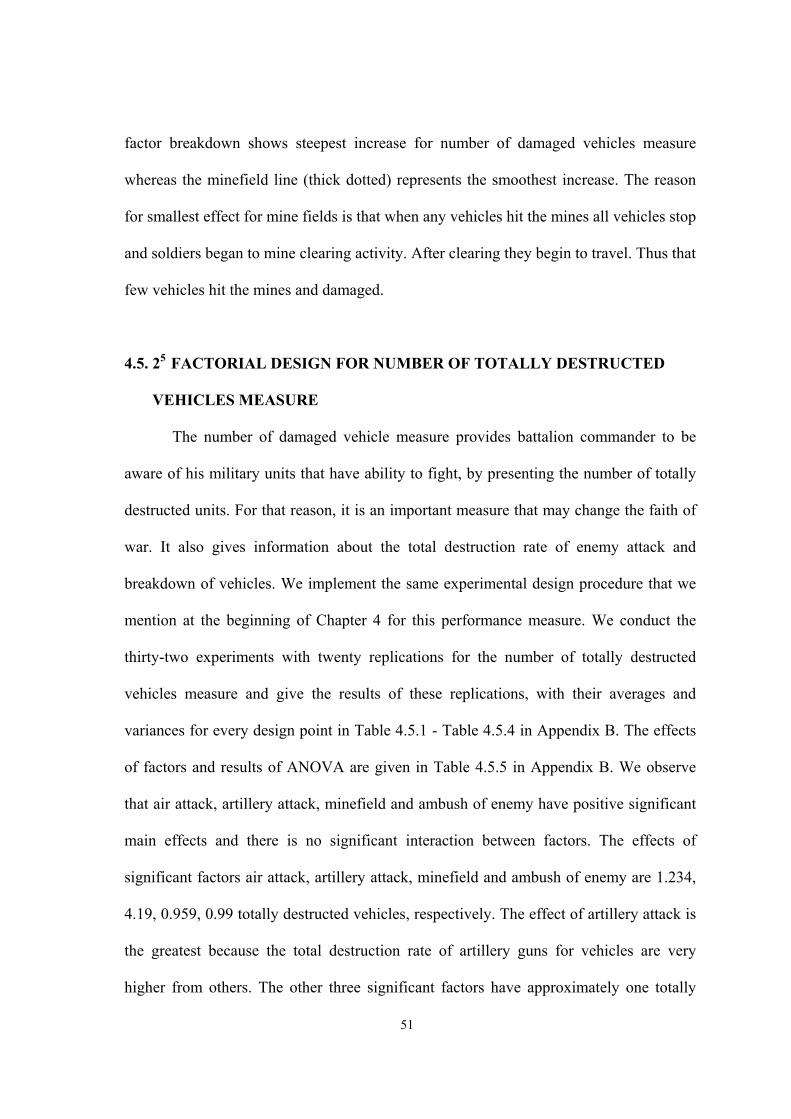
51
factor breakdown shows steepest increase for number of damaged vehicles measure
whereas the minefield line (thick dotted) represents the smoothest increase. The reason
for smallest effect for mine fields is that when any vehicles hit the mines all vehicles stop
and soldiers began to mine clearing activity. After clearing they begin to travel. Thus that
few vehicles hit the mines and damaged.
4.5. 25 FACTORIAL DESIGN FOR NUMBER OF TOTALLY DESTRUCTED
VEHICLES MEASURE
The number of damaged vehicle measure provides battalion commander to be
aware of his military units that have ability to fight, by presenting the number of totally
destructed units. For that reason, it is an important measure that may change the faith of
war. It also gives information about the total destruction rate of enemy attack and
breakdown of vehicles. We implement the same experimental design procedure that we
mention at the beginning of Chapter 4 for this performance measure. We conduct the
thirty-two experiments with twenty replications for the number of totally destructed
vehicles measure and give the results of these replications, with their averages and
variances for every design point in Table 4.5.1 - Table 4.5.4 in Appendix B. The effects
of factors and results of ANOVA are given in Table 4.5.5 in Appendix B. We observe
that air attack, artillery attack, minefield and ambush of enemy have positive significant
main effects and there is no significant interaction between factors. The effects of
significant factors air attack, artillery attack, minefield and ambush of enemy are 1.234,
4.19, 0.959, 0.99 totally destructed vehicles, respectively. The effect of artillery attack is
the greatest because the total destruction rate of artillery guns for vehicles are very
higher from others. The other three significant factors have approximately one totally
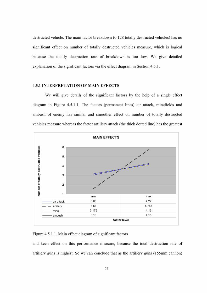
52
destructed vehicle. The main factor breakdown (0.128 totally destructed vehicles) has no
significant effect on number of totally destructed vehicles measure, which is logical
because the totally destruction rate of breakdown is too low. We give detailed
explanation of the significant factors via the effect diagram in Section 4.5.1.
4.5.1 INTERPRETATION OF MAIN EFFECTS
We will give details of the significant factors by the help of a single effect
diagram in Figure 4.5.1.1. The factors (permanent lines) air attack, minefields and
ambush of enemy has similar and smoother effect on number of totally destructed
vehicles measure whereas the factor artillery attack (the thick dotted line) has the greatest
MAIN EFFECTS
1
2
3
4
5
6
factor level
num
ber o
f tot
ally
des
truc
ted
vehi
cles
air attack 3,03 4,27
artillery 1,56 5,753
mine 3,175 4,13
ambush 3,16 4,15
min max
Figure 4.5.1.1. Main effect diagram of significant factors
and keen effect on this performance measure, because the total destruction rate of
artillery guns is highest. So we can conclude that as the artillery guns (155mm cannon)
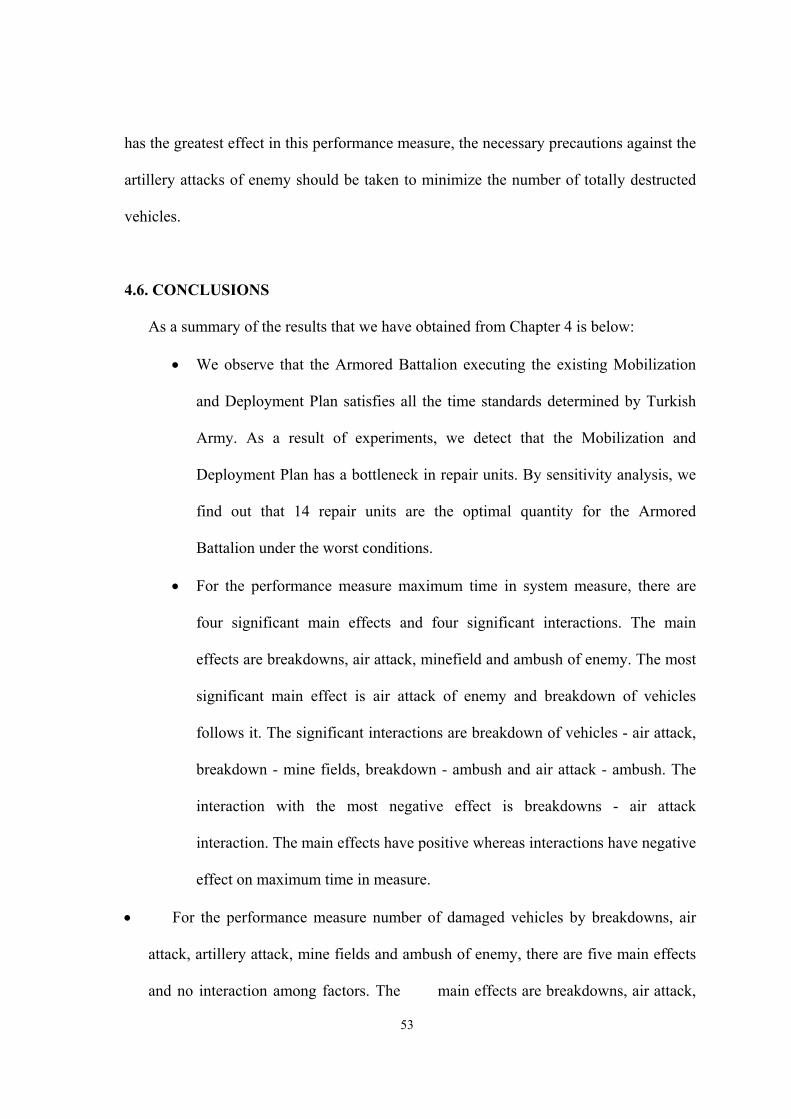
53
has the greatest effect in this performance measure, the necessary precautions against the
artillery attacks of enemy should be taken to minimize the number of totally destructed
vehicles.
4.6. CONCLUSIONS
As a summary of the results that we have obtained from Chapter 4 is below:
• We observe that the Armored Battalion executing the existing Mobilization
and Deployment Plan satisfies all the time standards determined by Turkish
Army. As a result of experiments, we detect that the Mobilization and
Deployment Plan has a bottleneck in repair units. By sensitivity analysis, we
find out that 14 repair units are the optimal quantity for the Armored
Battalion under the worst conditions.
• For the performance measure maximum time in system measure, there are
four significant main effects and four significant interactions. The main
effects are breakdowns, air attack, minefield and ambush of enemy. The most
significant main effect is air attack of enemy and breakdown of vehicles
follows it. The significant interactions are breakdown of vehicles - air attack,
breakdown - mine fields, breakdown - ambush and air attack - ambush. The
interaction with the most negative effect is breakdowns - air attack
interaction. The main effects have positive whereas interactions have negative
effect on maximum time in measure.
• For the performance measure number of damaged vehicles by breakdowns, air
attack, artillery attack, mine fields and ambush of enemy, there are five main effects
and no interaction among factors. The main effects are breakdowns, air attack,

54
artillery attack, minefield and ambush of enemy. The most significant main effect is
breakdown of vehicles and air attack of enemy follows it. All these factors have
positive effect on number of damaged vehicles measure.
• For the performance measure number of totally destructed vehicles by
breakdowns, air attack, artillery attack, mine fields and ambush of enemy, there are
four main effects and no interaction among factors. The main effects are air attack,
artillery attack, minefield and ambush of enemy. The most significant main effect is
artillery assault of enemy and air attack of enemy follows it. All these factors have
positive effect on number of damaged vehicles measure.
• In Chapter 4, we get general information about the attacks of enemy and
breakdown of vehicles for three different performance measures. This broad-
spectrum information can be evaluated in two ways. First one is using it for planning
of national defense by focusing on the necessary measures against the strongest
factors. The other one is usage of information for planning of military operations by
the Armored Battalion commanders. The significant factors are different for each
performance measure. For an Armored Battalion commander, the importance of
performance measures is changeable according to the type of military operation. If
the operation is an ambush-type operation, time is more important. If the operation is
a defense-type operation, then the number of totally destructed vehicles measure
arises as the most important statistic. So commanders may use the proper information
for his battalion to plan the military operations and take necessary precautions
against the significant factors. We give the summary table of significant factors and
interactions in Table 4.6.1.
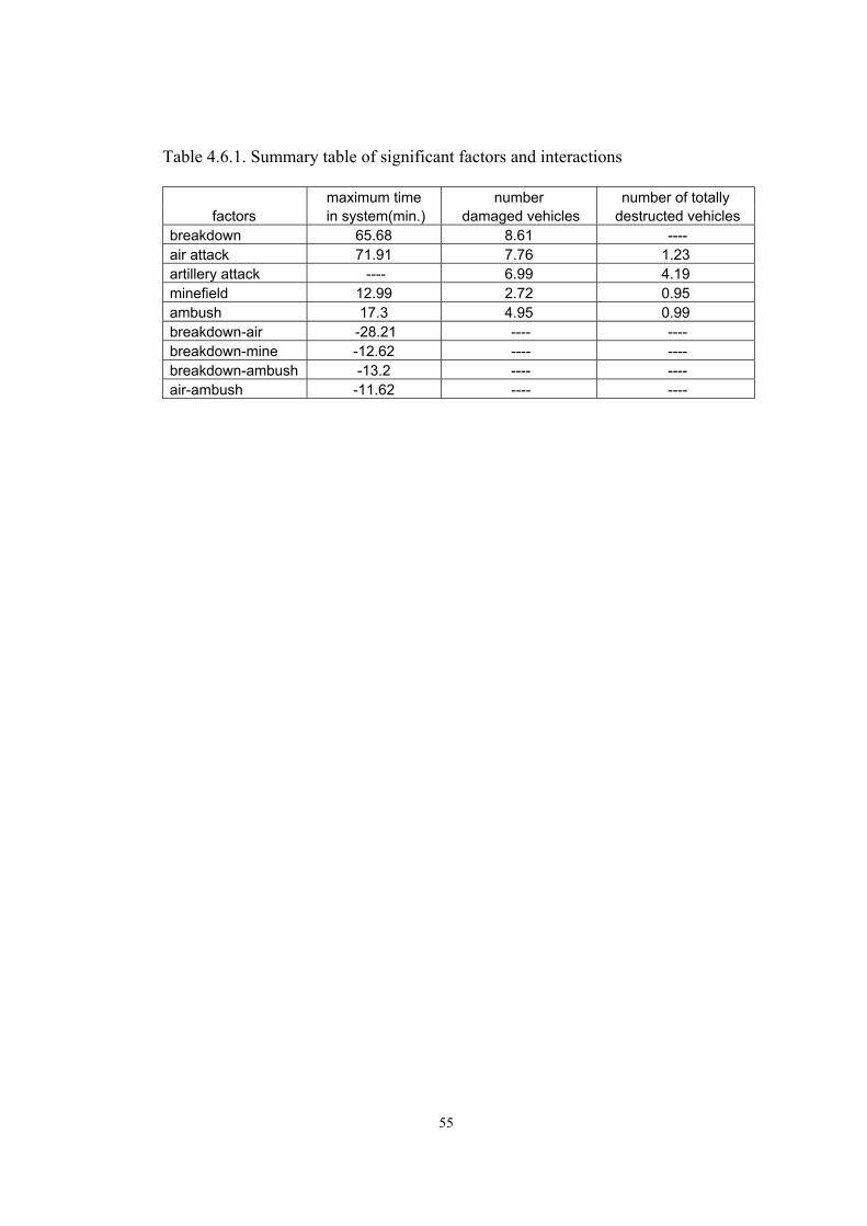
55
Table 4.6.1. Summary table of significant factors and interactions
maximum time number number of totally factors in system(min.) damaged vehicles destructed vehicles
breakdown 65.68 8.61 ---- air attack 71.91 7.76 1.23 artillery attack ---- 6.99 4.19 minefield 12.99 2.72 0.95 ambush 17.3 4.95 0.99 breakdown-air -28.21 ---- ---- breakdown-mine -12.62 ---- ---- breakdown-ambush -13.2 ---- ---- air-ambush -11.62 ---- ----

56
CHAPTER 5 5. SELECTING THE MOST CRITICAL REGION OF TURKEY
As a strategy, Turkish Army gives more importance to the troops in critical
regions. We can describe the regions in Turkey in three categories according to the
enemy threat.
• Eastern and South Eastern regions as most critical
• Aegean, Black Sea, Marmara, and Mediterranean as critical region
• Inside of Anatolia as least critical regions
The occurrence probabilities of enemy attacks and breakdown of vehicles are
different for each region. The troops in most critical regions have priority of having new
equipments and vehicles. The breakdown probabilities are determined according to the
condition of vehicles. Thus, the troops inside the Anatolia have higher breakdown
probabilities for breakdown station. Air attack, artillery attack, mine existing and ambush
probabilities are determined according to the power of neighbor country’s army, border
range with Turkey and the distance between that country and Turkey. The harm that the
enemy can cause depends on the power of its army. Border range is also an important
effect for combat. When the border is long, controlling the border will be hard. For that
reason, the probability of enemy penetrations, which can cause artillery assault,
minefields and ambush will increase. The distance between neighbor country and Turkey
also affects the condensation of artillery attack, minefield and ambush. For example,
between Russia and Turkey, the distance is very long because of Black Sea. For that
reason, artillery attack, mine existing and ambush probabilities are very low. Number of
totally destructed vehicles is higher in artillery attack, minefields and ambush than in air

57
attack and breakdown, because of the properties of guns and ground mines.
We compare the results of different regions according to the four performance
measures which are time in system of last vehicle arriving assembly area (maximum time
in system), average time in system, number of broken vehicles and number of totally
destructed vehicles. To be able to compare, we implement ranking and selection of
Rinott (1978) for selecting the most critique region among the ten regions of Turkey
from most to least critique according to the four performance measures. We prefer
Rinott’s procedure because it is more sensitive from others. It is used for the ranking and
selection of closer alternatives, because it needs more additional replications than the
other methods, and also needs less computation effort. We see that the rankings are
different from each other. To get a single ranking, we implement Saaty’s analytic
hierarchy process (AHP) (Winston, 1994). The Rinott’s ranking and selection process
can be implemented to the independent and normally distributed data. Our data is
normally distributed and independent. We check the normality of data in Chapter 4 and
use different random number generators for each random activity in our model to get
independent data. The steps of Rinott’s procedure are as follows:
Rinott’s Procedure:
STAGE 1:
We run 20 independent replications for each region.
We calculate average and variance of these replications for each region.
We find the sufficient number of replication for each region by the formula:
Ni = max {no, (h*Si/d)2}
STAGE 2:

58
We take Ni-no additional replications.
We calculate the average of Ni replications for each region.
Finally, we select the largest region as the most critique region among ten alternatives.
Our h value is 3.875 (from Table 8.3 (Rinott, 1978)) and desired probability of correct
selection is 0.95 for each performance measure whereas indifference amount differs.
5.1. SELECTING THE MOST CRITICAL REGION OF TURKEY ACCORDING
TO THE MAXIMUM TIME IN SYSTEM MEASURE
We implement the process above for the maximum time in measure of ten
regions. Our indifference amount d is 15 minutes for this performance measure. We
determine this d value by means inquiry that we give to the Armored Battalion and
Company commanders. The general opinion of commanders about the indifference
amount d is that the value depends on the type of operation and situation. We assume
that the Armored Battalion will execute a defense-type operation. Thus, the 15 minutes
indifference zone amount is reasonable for that type of operation. The results of twenty
replications, averages, variances and the sufficient replication number for Rinott’s
procedure are given in Table 5.1 – 5.2 in Appendix C.
After computing needed replication numbers, we take additional replications of
each region, and compute final averages of maximum time in measure for each region.
The final values (averages) are given in Table 5.1.1. We see that the average of the
results belonging to interior regions of Anatolia is lower than the others. It is logical
because the defense systems are more effective inner parts of Turkey. The most critical
regions are the Greece borders (Aegean and Trakya), and Southern East Region (Syria,

59
Iran and Iraq) borders follow them.
Table 5.1.1. Final averages of regions
no region average 1 Trakya Greece 329.35 2 Aegean 302.8 3 Syria 294.75 4 Iran 293.24 5 Iraq 292.06 6 Eastern Black Sea 278.61 7 Bulgaria 266.99 8 Middle Black Sea 233.06 9 Mediterranean 230.97 10 Middle Anatolia 223.12
The Greece border in Trakya is most critical because Greece Air Force is the
strongest one among other neighbors, and artillery units are very effective because of the
short distance between Turkey and Greece. Thus, these two strong factors cause more
damaged vehicles, which also increase the maximum time in measure.
5.2. SELECTING THE MOST CRITIQUE REGION OF TURKEY ACCORDING
TO THE AVERAGE TIME IN SYSTEM MEASURE
We apply the same process above for the average time in system measure of ten
regions. From the view of Armored Battalion commander, this performance measure
does not mean too much because, the important thing is when and with how many
vehicles Armored Battalion is ready in Assembly Area for combat. Thus, this
performance measure does not give necessary information about combat readiness. We
include this performance measure for only checking the average performance of our
system. Our indifference amount d is 15 minutes for this performance measure. The
reasoning in previous case for the determination of d value is also valid for this
performance measure. The results of twenty replications, averages, variances and

60
the sufficient replication number for Rinott’s procedure are given in Table 5.3 – 5.4 in
Appendix C. There is no need for additional replications indicated by the Rinott’s
procedure because the variances are so small. We can make a selection of the most
critique region by depending on averages of twenty replications. We give the summary
of averages in Table 5.2.1.
Table 5.2.1 Final averages of regions
no region average 1 Aegean 92.01 2 Trakya Greek 91.49 3 Iran 91.3 4 Syria 91 5 Iraq 90.4 6 Eastern Black Sea 89.7 7 Bulgaria 89.14 8 Mediterranean 82.97 9 Middle Black Sea 82.38 10 Middle Anatolia 80.04
We observe that the average of the results belonging to Middle of Anatolia is
lowest and Greece border in Aegean is the greatest. But there are very slight differences
between first seven regions in Table 5.2.1. Our indifference value d is 15 minutes for
average time in system measure, so we do not care about the selecting the most critique
system because the alternatives are too close to each other. We can say that the average
time in system measure does not give us necessary information about selecting the most
critique region. For that reason we do not include average time in system measure in
analytic hierarchy process (AHP) to find the most critique region among ten.
5.3. SELECTING THE MOST CRITICAL REGION OF TURKEY ACCORDING

61
TO THE NUMBER OF DAMAGED VEHICLES MEASURE
We determine indifference zone amount d from the inquiry as in previous case.
For the number of damaged vehicles our indifference amount d is 3 vehicles. We again
assume that operation is a defense-type operation. Three damaged vehicles can be
accepted as a reasonable value for a defense-type operation because the Armored
Battalion will occupy the predetermined position and wait for the enemy. Thus, there
may be enough time for repairing three vehicles before combat. We give the results of
twenty replications; averages, variances and the sufficient replication number for
Rinott’s procedure for the number of damaged vehicles measure are given in Table 5.5 –
5.6 in Appendix C. After taking additional replications needed, we present the final
averages in Table 5.3.1.
Table 5.3.1. Final averages of regions
no region average 1 Trakya Greek 25.45 2 Iraq 22.27 3 Bulgaria 22 4 Iran 21.9 5 Aegean 21.818 6 Eastern Black Sea 21.7 7 Syria 21.45 8 Mediterranean 12.27 9 Middle Black Sea 12.05 10 Middle Anatolia 9.75
The Greece border in Trakya is most dangerous and Middle Anatolia is the least
critical borders for this performance measure as in maximum time in system measure
case. The reasoning explained for that result in Section 5.1 is also valid. When number
of damaged vehicles increases, the maximum time in system measure naturally increases
because of the repairing times of damaged vehicles. We can say that there is a positive

62
correlation between these two performance measures. This relation is consistent with
results; the most and least critical regions for these two performance measures are the
same.
5.4 SELECTING THE MOST CRITICAL REGION OF TURKEY ACCORDING
TO THE NUMBER OF TOTALLY DESTRUCTED VEHICLES MEASURE
We put into practice the same ranking and selection procedure for number of
totally destructed vehicles measure, and give the results in Table 5.7 –5.8 in Appendix C.
Our indifference amount d takes the minimum value 1 vehicle. Because total destruction
of a vehicle means it cannot be used anymore, this is an important loss. After taking
additional replications needed, we give the final averages in Table 5.4.1.
Table 5.4.1 Final averages of regions
no region average 1 Iran 6.45 2 Syria 6.06 3 Trakya Greek 6.04 4 Bulgaria 5.626 5 Eastern Black Sea 5.59 6 Iraq 5.56 7 Aegean 5.3 8 Mediterranean 1.33 9 Middle Black Sea 1.21 10 Middle Anatolia 0.78
The Iran border is most critical because the Iran border is more suitable for
minefields; ambush and artillery assault whose total destruction rates are the highest.
These three strong factors cause more totally destructed vehicles, which also increase the
maximum time in measure. When a vehicle is totally destructed by the enemy, it is left in

63
a safe zone and this does not cause time loss. So we can say that there is no a direct
relation between maximum time in system and number of totally destructed vehicles
measure. The results that we obtain for these two are logical because results are different
as expected.
5.5. THE ANALYTIC HIERARCHY PROCESS
When we implement the ranking and selection process, we see that the rankings
of regions are different for each performance measure. For a decision maker, these three
performance measures are important. We have faced problem with a multiple objectives.
Thomas Saaty’s analytic hierarchy process (AHP) provides a powerful tool that can be
used to make decisions in situations involving multiple objectives (Winston, 1994). We
use AHP to make a single ranking of ten regions of Turkey according to the criteria of
criticism.
We describe an objective matrix of three performance measures by consulting the
military experts. The matrix is in Table 5.5.1.
Table 5.5.1 Objective matrix of three performance measures
objective matrix max time in # of damaged # of totally max time in 1 1.45 1.2 # of damaged 0.67 1 0.6 # of totally 0.83 1.67 1
And then by computing the normalized matrix of objective matrix, we get the
weights of each performance measures (Table 5.5.2).

64
Table 5.5.2 Normalized objective matrix and weights of performance measures
Norm(objective) max time in # of damaged # of totally weights max time in 0.4 0.351941748 0.428571 0.393504
# of damaged 0.268 0.242718447 0.214286 0.241668 # of totally 0.332 0.405339806 0.357143 0.364828
CONSISTENCY CHECK OF OBJECTIVE MATRIX
To check the consistency of our objective matrix, we implement the following procedure
(Winston, 1994):
Procedure:
Step1. We multiply the objective matrix with the transpose of the weights of
performance measures. A * wT
Step 2. We compute
1/n*Σ (ith entry of A * wT/ ith entry of wT)= 3.000419
Step 3. We compute the consistency index (CI) as:
CI= ((Step 2 results)-n)/n-1= 0.000209
Step 4. Finally, we compare the result with the theoric value (RI=0.58) in Table 23 of
Winston’s book (1994). For a perfectly consistent decision makers are probably
consistent enough to give useful estimates of weights for his objective function. We need
to check if CI/RI < 0.10. If CI/RI< 0.10, then we can say that the our objective matrix
is consistent. In our case,
CI/RI = 0.000209/0.58 = 0.000362 < 0.10
So we can say that our objective matrix is consistent, and we can continue implementing
AHP. We construct a 10*10 (10 regions) pair wise comparison matrix for each
performance measure by using the final results of ranking and selection procedure for
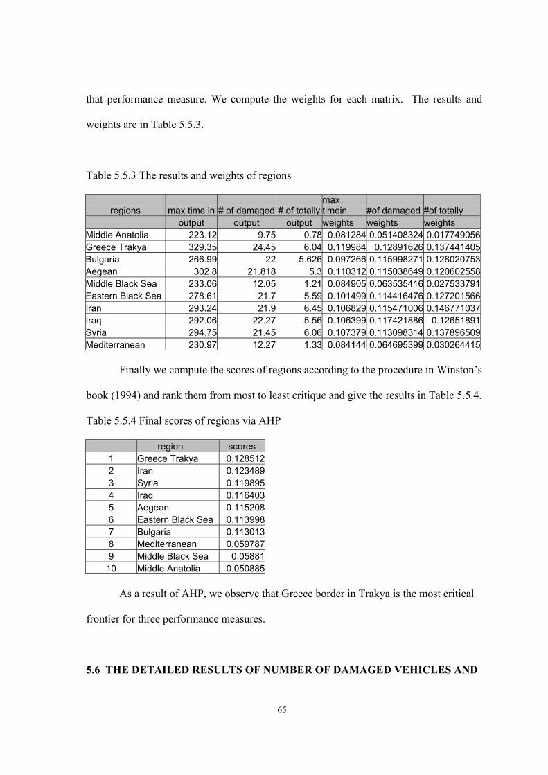
65
that performance measure. We compute the weights for each matrix. The results and
weights are in Table 5.5.3.
Table 5.5.3 The results and weights of regions
regions max time in # of damaged # of totally max timein #of damaged #of totally
output output output weights weights weights Middle Anatolia 223.12 9.75 0.78 0.081284 0.051408324 0.017749056 Greece Trakya 329.35 24.45 6.04 0.119984 0.12891626 0.137441405 Bulgaria 266.99 22 5.626 0.097266 0.115998271 0.128020753 Aegean 302.8 21.818 5.3 0.110312 0.115038649 0.120602558 Middle Black Sea 233.06 12.05 1.21 0.084905 0.063535416 0.027533791 Eastern Black Sea 278.61 21.7 5.59 0.101499 0.114416476 0.127201566 Iran 293.24 21.9 6.45 0.106829 0.115471006 0.146771037 Iraq 292.06 22.27 5.56 0.106399 0.117421886 0.12651891 Syria 294.75 21.45 6.06 0.107379 0.113098314 0.137896509 Mediterranean 230.97 12.27 1.33 0.084144 0.064695399 0.030264415
Finally we compute the scores of regions according to the procedure in Winston’s
book (1994) and rank them from most to least critique and give the results in Table 5.5.4.
Table 5.5.4 Final scores of regions via AHP
region scores 1 Greece Trakya 0.128512 2 Iran 0.123489 3 Syria 0.119895 4 Iraq 0.116403 5 Aegean 0.115208 6 Eastern Black Sea 0.113998 7 Bulgaria 0.113013 8 Mediterranean 0.059787 9 Middle Black Sea 0.05881
10 Middle Anatolia 0.050885
As a result of AHP, we observe that Greece border in Trakya is the most critical
frontier for three performance measures.
5.6 THE DETAILED RESULTS OF NUMBER OF DAMAGED VEHICLES AND

66
NUMBER OF TOTALLY DESTRUCTED VEHICLES MEASURE
We give the detailed results of the number of damaged and totally destructed
vehicles measure by partitioning them as the number of damaged vehicles by breakdown
of vehicles, the number of damaged vehicles by air attack, the number of damaged
vehicles by artillery attack, the number of damaged vehicles by minefields and the
number of damaged vehicles by ambush of enemy. These results are given to see how
many damaged vehicles or how much time delay do the factors cause for every scenario
separately. This type of information would be useful for the Armored Battalion
Commanders of regions that we inspect. Commanders can use this information for
effective planning of field exercises by focusing on the important factors. These statistics
are computed from the initial twenty replications only as information; we do not
implement any statistical procedure to make a comparison. We give the statistics of
wheeled trucks of Armored Battalion in Table 5.6.1-5.6.2, the number of damaged
armored vehicles measure in Table 5.6.3-5.6.4, the number of totally destructed wheeled
trucks measure in Table 5.7.1-5.7.2 and the number of totally destructed armored
vehicles measure in Table 5.7.3-5.7.4 in Appendix C.
5.7. CONCLUSIONS
In this chapter, we run our simulation model for armored battalions from ten
different regions of Turkey according to the four performance measures which are
maximum time in system, average time in system, number of damaged vehicles and
number of totally destructed vehicles. We implement Rinott’s ranking and selection
procedure (Rinott, 1978) to find out the most critical region for each performance
measure. For maximum time in system and number of damaged vehicles measures

67
Greece border in Trakya is the most critical whereas for the number of totally destructed
vehicle measure Iran, for the average time in system measure Aegean border of Greece is
the highest one. But we do not care about selecting the most critique system for that
performance measure because the alternatives are too close to each other.
For an Armored Battalion commander the number of totally destructed vehicles,
number of damaged vehicles and maximum time in system measures are very important.
However the average time in system measure does not imply a significant importance for
the military operations, because average time in system measure does not give sufficient
information about the whole battalion whereas maximum time in system points out the
readiness time of battalion for the combat. Except average time in system measure, we
implement analytic hierarchy process (AHP) to find out which region is the most critique
for the three performance measures. After implementation of AHP, we conclude that
Greece border in Trakya is the most critical region among ten regions of Turkey.
The information that we obtain in Chapter 5 may be used for planning of national
defense. According to our results, the defense planners should give the most importance
to Greece border in Trakya. For Iran border necessary precautions should be taken to
lessen the number of totally destructed vehicles, which is affected deeply from the
artillery guns, minefields, and ambushes of enemy.

68
CHAPTER 6
6. SELECTING THE MOST CRITICAL FACTOR FOR EACH REGION OF
TURKEY ACCORDING TO THE NUMBER OF TOTALLY DESTRUCTED
VEHICLES MEASURE
In Chapter 5, we implemented the ranking and selection procedure of Rinott
(1978) to find out which region of Turkey is most critical. In this chapter, we try to
discover which factor out of five is the most critical for each region. Again, we will use
the Rinott’s procedure only for number of totally destructed vehicles measure. The
information that other measures such as the maximum, average time in system measure
and number of damaged vehicles measures provide, is subjective, the indifference zone
amount for them may change depending on the type of military operation whereas the
indifference zone amount is always accepted as minimum number (1 vehicle)
independent of the type of military operation. At that point, the number of totally
destructed vehicles measure arises as an objective measure. Thus, we cannot reach
general conclusions for these three performance measures by performing ranking and
selection procedure while totally destructed vehicles measure can help us to reach exact
results for the degrees of criticism of five factors in the name of total destruction. Our
five factors are:
• Breakdowns of vehicles
• Air attack of enemy
• Artillery assault of enemy
• Mine field of enemy
• Ambush of enemy.
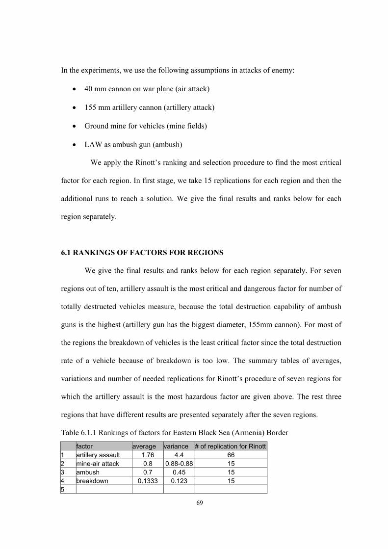
69
In the experiments, we use the following assumptions in attacks of enemy:
• 40 mm cannon on war plane (air attack)
• 155 mm artillery cannon (artillery attack)
• Ground mine for vehicles (mine fields)
• LAW as ambush gun (ambush)
We apply the Rinott’s ranking and selection procedure to find the most critical
factor for each region. In first stage, we take 15 replications for each region and then the
additional runs to reach a solution. We give the final results and ranks below for each
region separately.
6.1 RANKINGS OF FACTORS FOR REGIONS
We give the final results and ranks below for each region separately. For seven
regions out of ten, artillery assault is the most critical and dangerous factor for number of
totally destructed vehicles measure, because the total destruction capability of ambush
guns is the highest (artillery gun has the biggest diameter, 155mm cannon). For most of
the regions the breakdown of vehicles is the least critical factor since the total destruction
rate of a vehicle because of breakdown is too low. The summary tables of averages,
variations and number of needed replications for Rinott’s procedure of seven regions for
which the artillery assault is the most hazardous factor are given above. The rest three
regions that have different results are presented separately after the seven regions.
Table 6.1.1 Rankings of factors for Eastern Black Sea (Armenia) Border
factor average variance # of replication for Rinott 1 artillery assault 1.76 4.4 66 2 mine-air attack 0.8 0.88-0.88 15 3 ambush 0.7 0.45 15 4 breakdown 0.1333 0.123 15 5

70
Table 6.1.2 Rankings of factors for Iran border
factor average variance # of replication for Rinott 1 artillery assault 2.1 4.4 66 2 air attack 0.8 0.88-0.88 15 3 mine 0.7 0.45 15 4 ambush 0.1333 0.123 15 5 breakdown 0 0 15
Table 6.1.3 Rankings of factors for Iraq border
factor average variance # of replication for Rinott 1 artillery assault 1.68 3.73 42 2 air attack-ambush 1.2 0.6-0.622 15 3 mine 0.733 0.352 15 4 breakdown 0.0667 0.0667 15 5
Table 6.1.4 Rankings of factors for Syria border
factor average variance # of replication for Rinott 1 artillery assault 1.77 4.6 69 2 mine 1.2 1.028 15 3 air attack 0.8 0.6 15 4 ambush 0.5 0.5 15 5 breakdown 0 0 15
Table 6.1.5 Rankings of factors for Greece border in Trakya
factor average variance # of replication for Rinott 1 artillery attack 1.81 4.266 65 2 air attack 0.933 1.49 23 3 ambush 0.8 0.844 15 4 mine 0.6 0.4 15 5 breakdown 0 0 15
Table 6.1.6 Rankings of factors for Bulgaria border
factor average variance # of replication for Rinott 1 artillery attack 1.65 3.83 58 2 air attack 1.066 1.209 18 3 ambush 0.6 0.711 15 4 mine 0.533 0.69 15 5 usual break 0.0667 0.0667 15

71
Table 6.1.7 Rankings of factors for Greece border in Aegean
factor average variance # of replication for Rinott 1 artillery attack 1.58 4.12 62 2 air attack-mine 0.866 1.12-0.98 17-15 3 ambush 0.4 0.488 15 4 usual break 0 0 15 5
The ranking of factors for Mediterranean border is given in Table 6.1.8.
Minefield is the most, breakdown and artillery attack are least critical factors for this
border. Because of Mediterranean Sea the artillery attack probability is very low whereas
the minefield existing probabilities are higher because of guerilla activities of enemy and
total destruction rates of mines are very high. Thus, artillery attack and breakdown of
vehicles are the least risky factors for that region.
Table 6.1.8 Rankings of factors for Mediterranean border
factor average variance # of replication for Rinott 1 mine 0.6 0.54 15 2 air attack 0.33 0.238 15 3 ambush 0.3 0.45 15 4 breakdown-artillery 0 0 15 5
We give the average and variances of factors for Middle Anatolia in Table 6.1.9.
Air attack is the most critical factor because the most effective combat weapons for the
inner sides of countries are warplanes. The occurrence probabilities of other enemy
attacks are very low because defense is very effective for interior regions. The artillery
attack is the least critique because it is very hard even impossible for enemy to carry the
artillery guns inside the Anatolia to make an artillery assault against the interior sides.
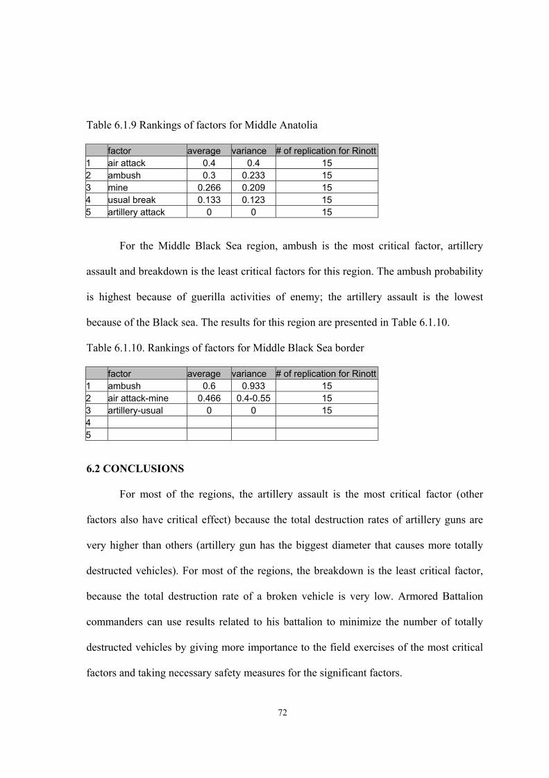
72
Table 6.1.9 Rankings of factors for Middle Anatolia
factor average variance # of replication for Rinott 1 air attack 0.4 0.4 15 2 ambush 0.3 0.233 15 3 mine 0.266 0.209 15 4 usual break 0.133 0.123 15 5 artillery attack 0 0 15
For the Middle Black Sea region, ambush is the most critical factor, artillery
assault and breakdown is the least critical factors for this region. The ambush probability
is highest because of guerilla activities of enemy; the artillery assault is the lowest
because of the Black sea. The results for this region are presented in Table 6.1.10.
Table 6.1.10. Rankings of factors for Middle Black Sea border
factor average variance # of replication for Rinott 1 ambush 0.6 0.933 15 2 air attack-mine 0.466 0.4-0.55 15 3 artillery-usual 0 0 15 4 5
6.2 CONCLUSIONS
For most of the regions, the artillery assault is the most critical factor (other
factors also have critical effect) because the total destruction rates of artillery guns are
very higher than others (artillery gun has the biggest diameter that causes more totally
destructed vehicles). For most of the regions, the breakdown is the least critical factor,
because the total destruction rate of a broken vehicle is very low. Armored Battalion
commanders can use results related to his battalion to minimize the number of totally
destructed vehicles by giving more importance to the field exercises of the most critical
factors and taking necessary safety measures for the significant factors.

73
CHAPTER 7
7. LIMITS OF MOBILIZATION AND DEPLOYMENT PLAN
To find out when our system collapse, we run the model under the worst enemy
threat. Up to now, our assumptions about the enemy forces were:
• 1 F-16 with 40 mm cannon on it
• 1 artillery platoon (4 155 mm artillery cannon)
• 6 ground mines for vehicles in an 8*8 mine field
• 4 LAW as ambush guns
We run our model for two scenarios. The assumptions and results for the worst two scenarios are stated below.
7.1 SCENARIO 1
Mobilization and Deployment Plan of a Turkish Armored Battalion is executed in
Turkish Land. Thus, the density of enemy threat that an Armored Battalion encounters
will be less than the threat in enemy land. The assumptions that we make up to this
Chapter 7 are reasonable for an operation in Turkish Land. As a military strategy, for an
armored battalion generally, one artillery platoon (4 cannons), for an ambush 4 LAWs,
for an 8*8 minefield 4 mines are assigned for assaulting against. To test the system under
worst conditions, we increase the density of enemy attack as much as possible. For
enemy it is unlikely to attack an armored battalion with 8 F-16 warplanes, one artillery
company, 8 LAWs in an ambush and a more condensed minefield. And also the
probability that all these enemy activities will occur together is very low. As our aim is
to find the system limits, we run our model under these worst conditions. The
assumptions are:

74
• 8 F-16 with 40 mm cannon on it
• 1 artillery company (8 155 mm artillery cannon)
• 12 ground mines for vehicles in 8*8 mine field
• 8 LAW as ambush guns
The results and variances of 20 replications are given in Table 7.1.1. For the Scenario
1, the average time in system statistic is 504.3 and maximum time in system statistic is
2009 minutes. Although there is no specific rule for the time delay of any military
operation, these measures are not reasonable for all kind of military operations. When we
look at the number of damaged vehicles, we see that 36 armored vehicles and 70-
wheeled trucks are damaged. These are also huge numbers for an armored battalion. Also
5 armored vehicles and 15-wheeled trucks are totally destructed by the enemy. Thus, we
can say that the Armored battalion in that condition cannot give proper reaction to
orders.
7.2 SCENARIO 2
For armored troops, the Apache helicopters are accepted as the most dangerous
enemy. Because they have hell-fire missiles that can hit a tank from 8000 meters with
0.55 shot probability. For the scenario 2, we just replace the F-16 warplanes with Apache
helicopters to observe the system performance. We make following assumptions for
Scenario 2:
• Apache helicopters with hell-fire missile on it
• 1 artillery company (8 155 mm artillery cannon)
• 12 ground mines for vehicles in an 8*8 mine field

75
• 8 LAW as ambush guns
We present the results of Scenario 2 in Table 7.2.1. The average and maximum time
in system statistics are 868.34 and 2558 minutes respectively. The number of damaged
armored vehicles and wheeled-trucks are 46 and 81 respectively. When we take a look at
the number of totally destructed vehicles, 17 wheeled-trucks and 6 armored vehicles are
totally destructed. The hell-fire missiles are more effective against armored forces; their
hit probabilities are very high. So as expected all the performance measures in Scenario 2
is higher than the ones in Scenario1.
Table 7.1.1 Results of Limit Scenario 1
8 F-16 (40 mm cannon), 8-155 mm cannons,12 mines, 8 LAWs average max damaged totally destructed time in timein tank vehicle total tank vehicle total
1 322.98 1545.64 40 55 95 2 11 13 2 502.04 1976.11 38 72 110 6 13 19 3 502.78 1920.16 39 70 109 5 12 17 4 456.91 1893.76 38 75 113 4 19 23 5 545.11 2341.43 33 75 108 4 14 18 6 295.56 1368.21 33 55 88 3 17 20 7 657.52 2620.02 32 75 107 3 12 15 8 779.55 2743.89 45 83 128 10 15 25 9 645.26 2629.47 28 79 107 5 14 19 10 431.31 1218.98 39 52 91 3 16 19 11 382.20 1704.73 35 60 95 2 15 17 12 403.04 1800.74 28 61 89 5 14 19 13 478.64 1744.60 42 63 105 9 15 24 14 629.08 2291 30 81 111 4 12 16 15 413.54 1897.56 39 73 112 8 20 28 16 479.93 2108.37 36 71 107 12 15 27 17 467.62 1915.66 34 67 101 3 13 16 18 600.12 2083.24 38 67 105 5 15 20 19 643.30 2337.15 41 78 119 2 20 22 20 450.95 2052.43 31 76 107 6 16 22
average 504.37 2009.66 35.95 69.4 105.35 5.05 14.9 19.95 variance 15143.0 163791.8 22.36 82.88 99.71 7.73 6.62 15.94

76
Table 7.2.1 Results of Limit Scenario 2
8 helicopter (hellfire). 8-155 mm cannons.12 mines. 8 LAWs average max damaged totally destructed time in timein tank vehicle total tank vehicle total
1 805.25 2460.06 50 78 128 12 18 30 2 1049.49 3112.88 44 93 137 6 14 20 3 929.40 2328.77 48 82 130 8 17 25 4 747.32 2105.57 51 73 124 4 16 20 5 833.65 1970.91 55 72 127 4 17 21 6 703.59 1717.28 43 58 101 3 16 19 7 821.06 2697.45 47 86 133 9 20 29 8 1004.76 3277.37 44 89 133 6 15 21 9 580.93 1800.67 44 64 108 6 15 21 10 1154.16 3364.48 52 102 154 6 18 24 11 749.42 1921.96 44 75 119 6 15 21 12 784.93 1976.90 39 64 103 5 15 20 13 1026.14 3300.79 49 88 137 9 14 23 14 1015.85 3123.13 45 94 139 6 18 24 15 619.36 1835.61 46 58 104 5 15 20 16 1026.52 3075.41 53 97 150 10 19 29 17 1013.91 3148.11 44 95 139 5 19 24 18 590.12 1627 43 58 101 3 16 19 19 946.28 3107.04 41 93 134 1 18 19 20 964.71 3209.29 40 90 130 4 13 17
average 868.34 2558.03 46.1 80.45 126.55 5.9 16.4 22.3 variance 28283.96 406874.2 19.46 206.26 251.20 6.93 3.72 13.37
7.3. CONCLUSIONS
Comparing the results of Scenario 2 with the Scenario 1 as seen in Table 7.3.1., the
performance measures of Scenario 2 are all greater than the measures of Scenario 1. We
also give the increase rates of performance measures for two scenarios in Table 7.3.2.
Table 7.3.1. Summary table of results of limit scenarios
average max damaged totally destructed scenario time in timein tank vehicle total tank vehicle total scenario 1 504.37 2009.66 35.95 69.4 105,35 5.05 14.9 19.95 scenario 2 868.34 2558.03 46.1 80.45 126.55 5.9 16.4 22.3
The maximum time in system statistic increase 13 times for Scenario1, whereas

77
17 times for Scenario 2. There is a % 63 increase in Scenario 1, %75 increase in Scenario
2 for the number of damaged vehicles measure. The increase rate in totally destructed
vehicles measure is %12 for Scenario 1 and % 13 for Scenario 2.
Table 7.3.2. Increase rates of performance measures
average max damaged totally destructed scenario time in (%) timein(%) tank(%) vehicle(%) total(%) tank(%) vehicle(%) total (%) scenario 1 522 1366 55 68 63 7 14 12 scenario 2 899 1738 71 79 75 9 16 13
As all the measures of Scenario 2 are greater, the enemy forces in Scenario 2 can be
accepted as limits that will put the Armored Battalion executing Mobilization and
Deployment Plan into a catastrophic situation. In other words, if enemy attacks an
Armored Battalion executing the Mobilization and Deployment Plan with 8 Apache
helicopters, one artillery company, lays an ambush with 8 LAW guns and positions a
minefield with density 12 anti-tank mines in a 8*8 m2, the Armored Battalion will get
into a mortal situation.
78
CHAPTER 8
CONCLUSIONS
8.1. GENERAL
In this study, we developed a simulation model of Mobilization and Deployment
of a Turkish Armored Battalion from garages to Assembly Area. We construct a flexible
model that can be also used for the Artillery and Infantry Battalion with slight
modifications. It can also be adapted to brigade-level Army Forces.
The objectives of our study are:
• To understand the behavior of existing Mobilization and Deployment Plan of an
Armored Battalion
• To find out the effects of enemy attacks on Armored Battalion
• To detect the bottlenecks of system if exist, and to develop solutions for
overcoming these problems
With our simulation model, we can test the system with different factors such as the
velocity of vehicles, the distance between garages and Alert Dispersion Area, the
distance between Alert Dispersion Area and Assembly Area, probability of breakdown
of vehicles, probability of air attack, probability of artillery assault, mine field existing
probability, ambush occurrence probability of enemy, the size of enemy forces (platoon,
company etc.).
In our study, we analyze the existing Mobilization and Deployment Plan of a Turkish
Armored Battalion; examine the effects of enemy attacks and breakdowns of vehicles,
select the most critical region out of ten region of Turkey, select the most critical factor
for each region according to the performance measures, maximum time in

79
system, number of damaged vehicles and number of totally destructed vehicles by five
factors. And finally find out limits of system for an Armored Battalion by running the
model at extreme conditions.
8.2. DESIGN AND ANALYSIS OF EXPERIMENTS
We test out the efficiency of the Mobilization and Deployment Plan of a Turkish
Armored Battalion by checking whether it satisfies time specifications of Turkish Army,
whether it has problem areas (bottlenecks). We also apply 2k factorial for observing the
effects of breakdown of vehicles, air attack, artillery assault, minefield, and ambush of
enemy according to the performance measures, maximum time in system, number of
damaged vehicles and number of totally destructed vehicles by five factors. We obtain
the results:
• As a result of experiments, we observe that the Armored Battalion executing the
existing Mobilization and Deployment Plan satisfies the all the time standards
determined by Turkish Army. But we discover that the Mobilization and
Deployment Plan has a bottleneck in number of repair units. 14 repair units are
the optimal quantity that minimizes the waiting time in queue statistic for the
Armored Battalion. Increasing the number of repair units from 5 to 14 in the
structure of the Armored Battalion will fix the bottleneck but may bring
additional cost.
• For the performance measure maximum time in system measure, the significant
effects are breakdowns of vehicles; air attack, minefield and ambush are 65.68,
71.91, 12.99, and 17.3 minutes respectively. There are also significant two-way
interactions between factors that we explain in Chapter 4. Effects of two-way

80
interactions of breakdowns- air attack, breakdowns- ambush, breakdowns-
minefields and air attack-ambush are –28.21, -13.2, -12.62 and –11.62 minutes,
respectively. Air attack has the greatest positive effect.
• For the number of damaged vehicles, there is no significant interaction among
factors. The significant effects of breakdowns of vehicles, air attack, artillery
assault, mine field and ambush are 8.6, 7.7, 6.99, 2.72, 4.96 vehicles respectively.
Breakdown of vehicles has the greatest effect.
• For the number of totally destructed vehicles, there is not a significant interaction
among factors either. There are four significant main effects. The significant
effects of air attack, artillery assault, minefield and ambush are 1.23, 4.19, 3.96,
and 0.99 vehicles respectively. Artillery assault has the greatest effect on this
performance measure.
The significant factors are different for each performance measure. For an Armored
Battalion commander, the importance of performance measures varies according to the
type of military operation. If the operation is an ambush-type operation, maximum time
in system measure is more important. If the operation is a defense-type operation, then
the number of totally destructed vehicles measure arises as the most important measure.
The information gained above can be also used for the Turkish national defense
planning: our study shows that the air attacks of enemy cause great delay for forward
military operation. To prevent this, the air defense system should be stronger. And also
breakdowns of vehicles are important factor for the maximum time in system measure
and number of damaged vehicle measure, which alert us to renew the vehicles for
decreasing reaction time of Armored Battalion for combat. We have to implement

81
preventative measures against the artillery assault of enemy to decrease the catastrophic
vehicle losses of Armored Battalion.
8.3. SELECTING THE MOST CRITICAL REGION OF TURKEY
We perform ranking and selection procedure for three performance measures. We get
different results for each performance measure. To find the most critical for three of
them we implement the analytic hierarchy process (AHP). The results are:
• The Greece border in Trakya is the most critical region for the performance
measure maximum time in system measure and number of damaged vehicles
whereas Iran is the most critical region for the performance measure number of
totally destructed vehicles.
• The result of AHP shows that the Greece border in Trakya is the most critical
region for three performance measures.
• Results reached in this chapter are high-level information that exceeds the
responsibilities of Armored Battalion commanders. This type of information can
be useful for the people who have the responsibility of planning the whole
defense system of Turkey. They should focus on Greece border in Trakya. For
Iran border necessary precautions should be taken to lessen the number of totally
destructed vehicles, which is affected intensely from the artillery guns,
minefields, and ambushes of enemy.

82
8.4. SELECTING THE MOST CRITICAL FACTOR FOR EACH REGIONS OF
TURKEY ACCORDING TO THE NUMBER OF TOTALLY DESTRUCTED
VEHICLES MEASURE
We execute ranking and selection procedure to select the most critical factor for
each region. For this purpose, we only use the number of totally destructed vehicles
measure to reach a general conclusion. The results are:
For most of the regions, artillery assault of enemy is the most critical factor and
breakdown arises as the least critical factor for the number of totally destructed vehicles
measure.
• This type of information can be used by the Armored Battalion commanders for
taking necessary precautions and the planning of field exercises against these five
factors. The commander should give more emphasis to the training against the
most critical factor for his region.
8.5. LIMITS OF MOBILIZATION AND DEPLOYMENT PLAN OF ARMORED
BATTALION
To find out when our system fails, we run the model under the worst enemy threat.
We observe after experiments that, if enemy attacks an Armored Battalion executing the
Mobilization and Deployment Plan with 8 Apache helicopters, one artillery company,
lays an ambush with 8 LAW guns and positions a minefield with density 12 anti-tank
mines in a 8*8 m2, the Armored Battalion will get into a mortal situation. We can
conclude that when the enemy attacks to an Armored Battalion with the force that we
stated below, enemy will cause the dead of battalion before getting into the battlefield.

83
Thus, the enemy forces mentioned below are the limits of the system.
8.6. CONCLUDING REMARKS
We draw following conclusions from our study:
• The existing Mobilization and Deployment Plan of Armored Battalion does not
have a serious problem during the movement from garages to Alert Dispersion
Area. Under the assumption that the vehicles are loaded before the alert order, it
satisfies the time limitations. But it needs a modification for the number of repair
units in structure of Armored Battalion.
• During the march from Alert Dispersion Area to Assembly Area there are five
significant factors that affect the performance of the Armored Battalion. The
factors are breakdowns of vehicles, air attack of enemy, artillery attack, mine
fields and ambushes of enemy. Only the breakdown of vehicles is the controllable
factor for Turkish Army. As it is a significant factor, the renewing of vehicle or
giving more emphasis on maintenance activites can decrease the effect of it. For
the other factors that are not controllable, the national defense system can be
strengthened to lessen the effects of them.
8.7. FUTURE RESEARCH TOPICS
Combat modeling is the most important issue in military. It is the modeling of
actions that may cause many casualties. By combat modeling, the military systems can
be examined with no losses and less cost. Simulation arises as one of the main tools of
combat modeling because terrain factors that the military operations continue and the
structure changes in military units can be the only issue to be handled by the simulation

84
to triumph over the problems.
We do not deal with the activities that are loading of ammunition and equipment
to wheeled trucks from depots and fuel oil filling of vehicles. These are also very
important factors that must be done before the alert order. A further study, including
these activities can be executed.
In our study, we make assumptions about the enemy forces and guns that are the
minor part of the whole alternatives. Thus, different types alternative scenarios can be
modeled for the Mobilization and Deployment Plan for future studies. And also we do
not deal with the terrain factors, the future studies may undertaken the terrain factors.
Our study considers the Mobilization and Deployment Plan of an Armored
Battalion. Future studies may consider the other types of battalions (infantry, artillery,
etc.) or the military units from different levels (brigade, company, etc.).
We take the vehicles of Armored Battalion as entities, so we only deal with the
vehicles in our study and evaluate the system in the name of vehicles. A more detailed
study that takes soldiers as entities may be conducted. We do not take care of the cost in
our study; this factor can be included in future studies.

85
APPENDIX A STRUCTURE OF A TURKISH ARMORED BATTALION
ARMORED BATTALION
Armored Company1
Armored Company2
Armored Company3
Headquarters And Headquarters Company

86
APPENDIX B
RESULTS OF 20 REPLICATIONS FOR EXPERIMENTAL DESIGN

87
Table 4.1. Factor names and roles of factors for design points Break(0.01-0.06) air(0-1) artillery(0-1) mine(0-1) ambush(0-1) design points
1 - - - - - run 2 + - - - - run1 3 - + - - - run2 4 - - + - - run3 5 - - - + - run4 6 - - - - + run5 7 + + - - - run12 8 + - + - - run13 9 + - - + - run14
10 + - - - + run15 11 - + + - - run23 12 - + - + - run24 13 - + - - + run25 14 - - + + - run34 15 - - + - + run35 16 - - - + + run45 17 + + + - - run123 18 + + - + - run124 19 + + - - + run125 20 + - + + - run134 21 + - + - + run135 22 + - - + + run145 23 - + + + - run234 24 - + + - + run235 25 - + - + + run245 26 - - - + + run345 27 + + + + - run1234 28 + + + - + run1235 29 + + - + + run1245 30 + - + + + run1345 31 - + + + + run2345 32 + - + + + run12345

88
Table 4.3.1. Results. averages and variances of 20 replications for maximum time in
run 0 run1 run2 run3 run4 run5 run12 run13 1 159 418 351.5 201.98 347.16 222.27 379 372 2 149 286 280.24 157.15 162.69 225.27 284 272 3 145 277 209.38 163.35 254.36 229.31 327 313 4 161 365 373.88 180.32 231.04 256.67 301 309 5 115 227 315.76 186.15 223.58 351.82 233 263 6 103 335 347.2 213.32 368.11 237.07 302 450 7 147 198 325.32 207.91 162.81 178.2 421 170 8 111 330 225.94 158.4 147.99 203.5 458 478 9 137 297 366.09 185.59 199.49 207.07 452 300
10 164 299 351.37 189.08 166.13 236.87 427 390 11 177 302 326.39 191.72 191.79 192.65 326 341 12 199 327 402.6 280.17 204.78 183.1 390 215 13 141 343 188.64 154.19 217.45 235.38 303 353 14 104 246 198.72 290.45 194.74 271.92 283 259 15 179 280 222.7 157.49 144.34 253.54 264 331 16 105 206 211.22 201.39 250.63 160.28 442 270 17 225 259 245.78 192.63 184.79 246.66 293 220 18 102 353 287.07 210.75 194.94 279.58 288 257 19 128 334 393.55 224.5 352.56 316.27 487 345 20 191 319 355.93 163.41 180 254.64 446 261
average 147.1 300.05 298.964 195.4975 218.969 237.1035 17.85 16.45 variance 1246.095 3025.418 5001.383 1386.733 4412.529 2116.553 6126.747 5915.524 Table 4.3.2. Results. averages and variances of 20 replications for maximum time in
run14 run15 run23 run 24 run25 run34 run35 run45 1 366 399.59 390.98 314.43 355.56 261.36 164.39 348.68 2 265 234.45 323.37 331.32 307.77 199.8 225.3 261.03 3 313 297.16 239.82 247.51 222 258.37 258.59 216.62 4 338 360.62 262.86 350.66 240.53 169.96 174.44 185.29 5 247 365.25 338.86 265.98 343.05 244.54 368.35 308.69 6 380 434.94 279.91 376.19 328.89 362.79 183.65 357.14 7 238 209.01 262.28 408.86 308.26 207.41 278.56 159.64 8 382 459.87 309.83 380.43 307.96 219.03 214.49 252.05 9 338 333.18 486.13 364.73 435.16 173.04 242.43 236.85
10 308 283.25 445.13 468.4 450.8 227.71 193.08 210.2 11 305 302.2 309.61 219.59 348.81 247.36 213.3 192.18 12 282 249.74 397.65 338.86 325.78 273.26 247.49 203.25 13 384 414.41 298.32 293.87 304.95 270.83 228.35 227.49 14 250 268.07 307.53 238.38 239.4 206.99 189.28 256.6 15 401 336.89 212.81 247.97 207.62 163.74 204.44 206.96 16 335 297.58 208.68 250.5 208.87 177.88 235.25 237.89 17 218 230.75 278.1 277.77 349.56 286.91 264.42 275.12 18 300 365.52 359.14 260.81 289.29 151.71 218.78 253.35 19 453 314.29 367.01 392.44 479.81 372.1 236.64 320.36 20 253 270.61 257.51 375.4 449.07 173.95 206.52 220.09
average 317.8 321.369 316.7765 320.205 325.157 232.437 17.85 16.45 variance 3990.274 4979.673 5433.551 4705.497 6560.31 3794.19 2017.493 2859.336

89
Table 4.3.3. Results. averages and variances of 20 replications for maximum time in
run123 run124 run125 run134 run135 run145 run 234 run235 1 372.76 407.89 364.05 412.94 356.68 355.01 324.14 303.17 2 334.19 342.28 327.38 330.75 343.49 369.19 363.18 281.15 3 480.29 309.04 374.44 298.22 244.12 368.77 320.18 219.33 4 419.17 394.93 420.66 338.89 353.85 324.65 219.88 321.01 5 305.91 390.29 412.16 306.79 312.89 367.36 250.79 352.56 6 381.64 331.01 321.77 470.57 378.16 347.44 355.1 321.99 7 331.51 361.76 385.23 200.57 256.33 231.43 339.45 405.24 8 347.41 361.91 337.58 366.31 422.87 267.48 366.19 288.78 9 329.67 372.79 404.04 306.21 317.11 276.47 362.41 389.42
10 545.24 375.18 530.3 241 262.55 296.69 443.79 561.14 11 306.65 318.81 320.91 285.58 320.87 296.06 326 259.39 12 410.33 311.51 383.37 396.45 417.33 205.61 419.75 373.01 13 376.54 347.68 389.42 380.62 407.93 373.23 360.05 287.63 14 370.85 259.98 260.25 266.44 263.66 319.96 252.04 237.54 15 350.08 448.74 294.07 230.92 368.36 380.55 275.18 267.21 16 352.24 286.46 215.16 298.77 320.94 257.69 202.92 263.6 17 288.94 354.04 241.5 261.84 327.52 333.48 263.56 349.56 18 302.46 333.32 278.83 295.22 271.2 312.07 281.86 286.56 19 420.03 412.11 363.33 328.94 346.33 354.14 398.93 481.58 20 384.63 463.46 482.75 240.93 254.49 303.42 356.49 287.16
average 370.527 359.1595 355.36 312.898 327.334 317.035 17.85 16.45 variance 3930.591 2643.283 6038.194 4555.176 3118.174 2506.963 4281.769 6986.258 Table 4.3.4. Results. averages and variances of 20 replications for maximum time in
run245 run345 run1234 run1235 run1245 run1345 run2345 run12345 1 341.75 401.15 437.2 381.48 448.66 431.66 349 361.53 2 278.8 272.86 342.54 342.95 377.49 340.17 333.83 387.12 3 219.44 278.78 307 370.15 219.85 357.08 224.13 359.32 4 338.16 297.17 383.9 344.51 478.6 345.62 318.35 411.48 5 436.04 348.32 400.1 367.48 473.63 414.13 442.12 396.59 6 342.24 313.46 398.57 322.48 370.13 336.09 320.76 356.06 7 279.53 214.58 344.21 384.04 419.55 270.85 381.08 337.71 8 302.66 328.17 406.14 382.16 321.14 269.47 270.52 443.96 9 386.46 216.71 393.91 432.26 414.03 302.41 304.76 454.58
10 529.93 270.38 409.77 470.01 439.46 324.06 484.79 434.83 11 271.05 200.13 315.25 325.62 296.58 323.58 244.88 347.05 12 466.72 231.34 356.9 328.91 316.96 266.3 417.82 350.33 13 358.59 288.86 374.87 397.61 378.01 390.73 343.7 384.32 14 282.56 195.04 277.44 235.47 271.79 227.3 233.51 307.5 15 253.15 159.89 321.22 267.31 274.2 233.39 249.51 279.44 16 229.22 192.36 212.93 310.58 311.41 193.85 287.32 295.33 17 351.51 316.38 336.94 298.15 295.65 282.45 344.21 335.89 18 271.54 338.47 267.87 360.83 278.48 263.14 321.98 284.85 19 387.77 347.61 433.54 383.44 403.1 393.54 371.66 380.09 20 393.24 198.46 398.12 381.9 387.88 380.88 335.28 316.36
average 336.018 270.506 355.921 354.367 358.83 317.335 17.85 16.45 variance 6562.572 4411.6 3498.781 2909.293 5593.41 4360.184 4730.749 2611.693

90
Table 4.3.5. Effects and Results of Analysis of Variance for maximum time in system statistic source of variation average effect SSx df MSx Fo
1 300.5 65.68275 690275.7836 1 690275.78 167.9404 significant 2 298.96 71.91 827367.696 1 827367.7 201.2941 significant 3 195.48 7.259 8430.89296 1 8430.893 2.051191 insignificant 4 218.5 12.99 26998.416 1 26998.416 6.568569 significant 5 237.1 17.3 47886.4 1 47886.4 11.6505 significant 12 355.39 -28.21 127328.656 1 127328.66 30.97838 significant 13 308.43 -4.24 2876.416 1 2876.416 0.699817 insignificant 14 317.8 -12.62 25482.304 1 25482.304 6.199708 significant 15 321.36 -13.2 27878.4 1 27878.4 6.782665 significant 23 316.76 -3.47 1926.544 1 1926.544 0.468718 insignificant 24 320.2 -8.024 10301.53216 1 10301.532 2.506307 insignificant 25 325.08 -11.62 21603.904 1 21603.904 5.256114 significant 34 232.38 -3.64 2119.936 1 2119.936 0.515769 insignificant 35 227.37 -5.14 4227.136 1 4227.136 1.028439 insignificant 45 246.47 -5.401 4667.32816 1 4667.3282 1.135536 insignificant
123 371.014 4.16 2768.896 1 2768.896 0.673658 insignificant 124 359.15 6.99 7817.616 1 7817.616 1.901984 insignificant 125 355.36 4.861 3780.69136 1 3780.6914 0.919822 insignificant 134 312.87 -0.59 55.696 1 55.696 0.013551 insignificant 135 327.36 4.31 2972.176 1 2972.176 0.723114 insignificant 145 317 3.611 2086.29136 1 2086.2914 0.507583 insignificant 234 324.01 -1.231 242.45776 1 242.45776 0.058989 insignificant 235 326.83 0.433 29.99824 1 29.99824 0.007298 insignificant 245 336 6.09 5934.096 1 5934.096 1.443734 insignificant 345 270.5 6.389 6531.09136 1 6531.0914 1.588979 insignificant 1234 355.89 1.631 425.62576 1 425.62576 0.103552 insignificant 1235 354.8 -2.09 698.896 1 698.896 0.170038 insignificant 1245 358.81 1.15 211.6 1 211.6 0.051481 insignificant 1345 317.33 -2.686 1154.33536 1 1154.3354 0.280844 insignificant 2345 328.1 -3.04 1478.656 1 1478.656 0.359749 insignificant
12345 361.8 4.947 3915.64944 1 3915.6494 0.952656 insignificant error 2499028.882 608 4110.2449 total 4368504 639

91
Table 4.4.1. Results. averages and variances of 20 replications for number of damaged vehicles
run0 run1 run2 run3 run4 run5 run12 run13 1 2 13 8 10 6 6 16 21 2 2 11 6 6 3 4 17 16 3 3 11 5 12 8 9 14 20 4 2 9 10 9 6 8 16 18 5 1 8 5 6 3 9 17 13 6 0 13 8 13 5 7 20 23 7 1 4 9 8 3 6 14 11 8 1 13 7 7 4 8 25 21 9 1 9 10 6 4 5 22 16 10 2 12 12 9 3 6 24 20 11 2 10 7 9 3 4 20 19 12 2 10 8 10 2 4 18 13 13 2 13 10 12 8 5 23 19 14 0 10 5 6 1 8 11 14 15 4 9 6 7 2 6 14 13 16 0 6 2 6 3 4 16 13 17 5 7 6 11 4 6 13 15 18 0 10 4 5 6 7 16 11 19 1 13 10 9 7 7 23 20 20 4 12 10 9 2 9 18 13
average 1.75 10.15 7.4 8.5 4.15 6.4 17.85 16.45 variance 1.986842 6.45 6.463158 5.526316 4.239474 2.989474 15.71316 13.94474
Table 4.4.2. Results. averages and variances of 20 replications for number of damaged vehicles
run14 run15 run23 run24 run25 run34 run35 run45 1 17 17 19 15 15 14 13 10 2 14 14 12 10 11 8 11 7 3 14 14 17 12 12 18 19 12 4 16 19 19 13 17 13 13 9 5 12 20 11 10 16 9 15 12 6 19 22 19 13 13 17 17 8 7 7 10 20 12 16 10 13 6 8 15 22 17 10 15 11 15 11 9 13 18 18 14 16 9 11 8 10 12 14 20 16 18 10 12 8 11 12 14 17 12 12 10 11 7 12 10 11 18 15 16 10 15 8 13 18 16 17 15 12 14 13 10 14 10 14 13 6 12 8 11 9 15 14 15 11 10 10 7 7 5 16 12 11 12 11 10 6 12 8 17 9 11 22 12 22 16 19 12 18 13 17 14 12 15 7 11 12 19 20 18 19 17 17 15 15 10 20 9 14 18 16 22 11 12 11
average 13.3 15.55 16.65 12.55 14.85 11.15 13.25 9.15 variance 12.11579 12.57632 10.87105 7.207895 11.81842 12.34474 8.513158 4.45
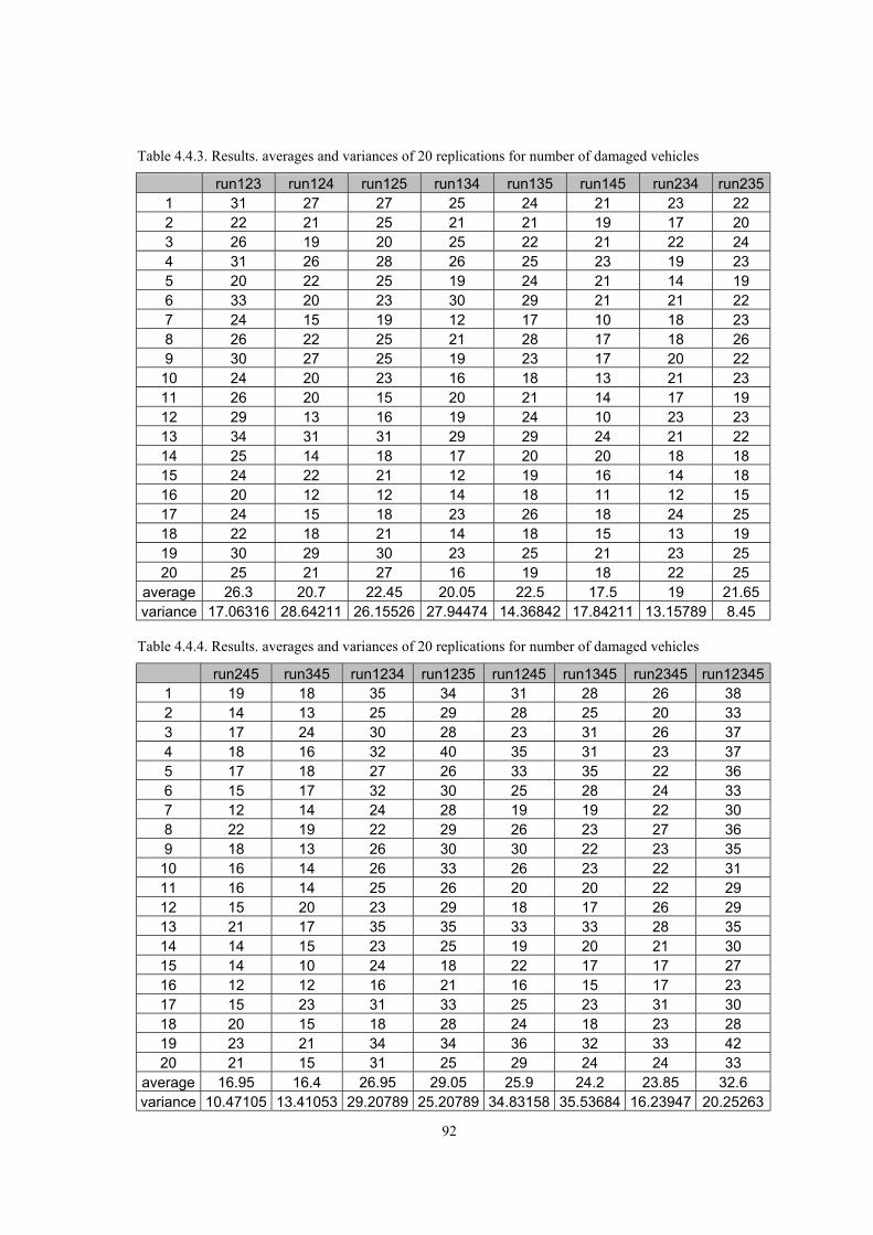
92
Table 4.4.3. Results. averages and variances of 20 replications for number of damaged vehicles
run123 run124 run125 run134 run135 run145 run234 run235 1 31 27 27 25 24 21 23 22 2 22 21 25 21 21 19 17 20 3 26 19 20 25 22 21 22 24 4 31 26 28 26 25 23 19 23 5 20 22 25 19 24 21 14 19 6 33 20 23 30 29 21 21 22 7 24 15 19 12 17 10 18 23 8 26 22 25 21 28 17 18 26 9 30 27 25 19 23 17 20 22
10 24 20 23 16 18 13 21 23 11 26 20 15 20 21 14 17 19 12 29 13 16 19 24 10 23 23 13 34 31 31 29 29 24 21 22 14 25 14 18 17 20 20 18 18 15 24 22 21 12 19 16 14 18 16 20 12 12 14 18 11 12 15 17 24 15 18 23 26 18 24 25 18 22 18 21 14 18 15 13 19 19 30 29 30 23 25 21 23 25 20 25 21 27 16 19 18 22 25
average 26.3 20.7 22.45 20.05 22.5 17.5 19 21.65 variance 17.06316 28.64211 26.15526 27.94474 14.36842 17.84211 13.15789 8.45
Table 4.4.4. Results. averages and variances of 20 replications for number of damaged vehicles
run245 run345 run1234 run1235 run1245 run1345 run2345 run12345 1 19 18 35 34 31 28 26 38 2 14 13 25 29 28 25 20 33 3 17 24 30 28 23 31 26 37 4 18 16 32 40 35 31 23 37 5 17 18 27 26 33 35 22 36 6 15 17 32 30 25 28 24 33 7 12 14 24 28 19 19 22 30 8 22 19 22 29 26 23 27 36 9 18 13 26 30 30 22 23 35
10 16 14 26 33 26 23 22 31 11 16 14 25 26 20 20 22 29 12 15 20 23 29 18 17 26 29 13 21 17 35 35 33 33 28 35 14 14 15 23 25 19 20 21 30 15 14 10 24 18 22 17 17 27 16 12 12 16 21 16 15 17 23 17 15 23 31 33 25 23 31 30 18 20 15 18 28 24 18 23 28 19 23 21 34 34 36 32 33 42 20 21 15 31 25 29 24 24 33
average 16.95 16.4 26.95 29.05 25.9 24.2 23.85 32.6 variance 10.47105 13.41053 29.20789 25.20789 34.83158 35.53684 16.23947 20.25263
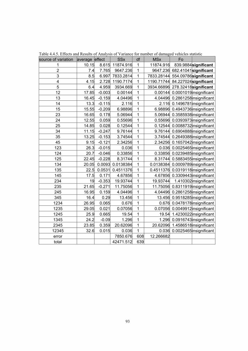
93
Table 4.4.5. Effects and Results of Analysis of Variance for number of damaged vehicles statistic source of variation average effect SSx df MSx Fo
1 10.15 8.615 11874.916 1 11874.916 839.9884 significant 2 7.4 7.765 9647.236 1 9647.236 682.41041 significant 3 8.5 6.997 7833.2814 1 7833.28144 554.09786 significant 4 4.15 2.728 1190.7174 1 1190.71744 84.227024 significant 5 6.4 4.959 3934.669 1 3934.66896 278.32418 significant 12 17.85 -0.003 0.00144 1 0.00144 0.0001019 insignificant 13 16.45 -0.159 4.04496 1 4.04496 0.2861258 insignificant 14 13.3 -0.115 2.116 1 2.116 0.1496781 insignificant 15 15.55 -0.209 6.98896 1 6.98896 0.4943736 insignificant 23 16.65 0.178 5.06944 1 5.06944 0.3585938 insignificant 24 12.55 0.059 0.55696 1 0.55696 0.0393973 insignificant 25 14.85 0.028 0.12544 1 0.12544 0.0088732 insignificant 34 11.15 -0.247 9.76144 1 9.76144 0.6904888 insignificant 35 13.25 -0.153 3.74544 1 3.74544 0.2649388 insignificant 45 9.15 -0.121 2.34256 1 2.34256 0.1657042 insignificant
123 26.3 -0.015 0.036 1 0.036 0.0025465 insignificant 124 20.7 -0.046 0.33856 1 0.33856 0.0239485 insignificant 125 22.45 -0.228 8.31744 1 8.31744 0.5883455 insignificant 134 20.05 0.0093 0.0138384 1 0.0138384 0.0009789 insignificant 135 22.5 0.0531 0.4511376 1 0.4511376 0.0319118 insignificant 145 17.5 0.171 4.67856 1 4.67856 0.3309443 insignificant 234 19 -0.353 19.93744 1 19.93744 1.410302 insignificant 235 21.65 -0.271 11.75056 1 11.75056 0.8311919 insignificant 245 16.95 0.159 4.04496 1 4.04496 0.2861258 insignificant 345 16.4 0.29 13.456 1 13.456 0.9518285 insignificant 1234 26.95 0.065 0.676 1 0.676 0.0478178 insignificant 1235 29.05 0.021 0.07056 1 0.07056 0.0049912 insignificant 1245 25.9 0.665 19.54 1 19.54 1.4230022 insignificant 1345 24.2 -0.09 1.296 1 1.296 0.0916743 insignificant 2345 23.85 0.359 20.62096 1 20.62096 1.4586518 insignificant
12345 32.6 0.015 0.036 1 0.036 0.0025465 insignificant error 7850.676 608 12.266682 total 42471.512 639

94
Table 4.5.1. Results. averages and variances of 20 replications for number of totally destructed vehicles
run0 run1 run2 run3 run4 run5 run12 run13 1 1 0 0 7 2 3 1 5 2 0 0 1 3 1 0 2 3 3 0 0 1 8 2 1 1 4 4 0 0 1 4 3 1 1 7 5 0 1 0 2 0 2 0 2 6 0 0 0 7 0 2 1 3 7 0 0 1 4 0 1 2 5 8 0 2 4 5 2 2 1 5 9 0 0 3 3 0 1 3 3
10 0 0 3 5 0 1 2 4 11 0 1 0 4 0 1 1 3 12 0 0 1 4 1 1 1 6 13 0 0 4 8 2 0 3 4 14 0 0 1 1 0 1 0 3 15 0 0 0 3 1 0 0 3 16 0 0 0 2 0 1 1 3 17 0 0 2 5 1 1 0 8 18 0 0 0 1 3 0 1 3 19 0 0 2 3 1 0 1 4 20 0 0 2 5 0 1 1 3
average 0.05 0.2 1.3 4.2 0.95 1 1.15 4.05 variance 0.05 0.273684 1.8 4.378947 1.102632 0.631579 0.765789 2.365789
Table 4.5.2. Results. averages and variances of 20 replications for number of totally destructed vehicles
run14 run15 run23 run24 run25 run34 run35 run45 1 1 1 6 1 0 8 10 2 2 1 3 3 1 2 3 3 1 3 2 0 8 3 2 8 3 2 4 2 2 5 3 5 7 4 3 5 1 1 2 2 2 3 5 4 6 0 1 10 1 1 6 10 2 7 0 0 7 0 2 3 4 1 8 2 1 5 0 4 6 4 3 9 1 1 5 3 4 4 4 3 10 0 1 4 1 2 3 6 2 11 1 2 1 1 2 3 3 1 12 1 0 6 3 2 5 5 1 13 1 2 6 3 1 5 4 3 14 1 3 1 1 2 3 7 2 15 0 0 4 1 3 5 2 2 16 2 0 3 0 0 3 3 2 17 0 0 7 2 2 7 6 1 18 1 1 4 5 2 5 5 3 19 0 0 7 5 0 6 7 1 20 1 0 8 3 3 5 3 2
average 0.9 0.95 5.1 1.95 2.05 4.9 4.9 2.05 variance 0.515789 0.997368 5.778947 2.260526 1.734211 3.042105 4.936842 0.786842

95
Table 4.5.3. Results. averages and variances of 20 replications for number of totally destructed vehicles
run123 run124 run125 run134 run135 run145 run234 run235 1 6 1 1 7 5 2 7 6 2 4 2 1 5 3 1 5 6 3 3 2 2 7 8 4 6 9 4 7 3 4 6 5 1 7 4 5 5 0 2 6 4 4 3 7 6 7 2 1 7 7 1 7 9 7 7 0 2 5 5 0 4 8 8 4 2 2 5 4 5 5 8 9 5 3 4 3 4 2 7 7 10 3 3 2 5 3 3 7 5 11 8 1 0 6 3 0 4 4 12 8 3 2 5 6 0 9 8 13 8 6 3 9 10 4 6 5 14 9 3 3 5 5 2 7 6 15 4 3 1 5 3 0 4 6 16 4 1 1 5 3 0 3 6 17 7 0 5 6 9 2 8 4 18 4 3 3 2 6 2 4 6 19 6 3 4 5 3 2 7 6 20 6 0 2 5 4 0 9 8
average 5.75 2.05 2.25 5.45 5 1.75 5.95 6.4 variance 3.355263 2.260526 1.671053 2.155263 4.421053 2.513158 3.418421 2.463158 Table 4.5.4. Results. averages and variances of 20 replications for number of totally destructed vehicles
run245 run345 run1234 run1235 run1245 run1345 run2345 run12345 1 1 6 6 5 3 9 6 6 2 5 4 3 5 1 4 4 4 3 3 10 9 4 9 8 7 13 4 6 6 7 10 4 6 8 9 5 3 7 8 4 6 7 7 7 6 0 6 5 7 0 6 11 8 7 3 5 7 5 1 4 7 8 8 4 8 4 7 2 6 9 8 9 3 6 6 10 6 7 10 11
10 0 5 7 4 3 4 5 5 11 4 6 8 5 2 6 8 6 12 2 8 11 8 3 5 11 10 13 1 5 7 6 4 6 4 8 14 4 7 6 12 1 6 10 7 15 3 5 7 2 5 4 2 4 16 2 6 5 6 1 8 6 5 17 2 10 7 9 2 8 8 10 18 3 6 7 5 4 4 8 5 19 7 5 4 7 6 7 11 6 20 3 5 8 8 5 4 6 12
average 2.95 6.3 6.6 6.45 3.4 5.95 7.4 7.6 variance 3.207895 2.642105 3.410526 6.155263 5.2 2.576316 6.357895 6.778947

96
4.5.5. Effects and Analysis of Variance for number of totally destructed vehicles statistic source of variation averages effect SSx df MSx Fo
1 0.2 0.128 2.62144 1 2.62144 0.93115 insignificant 2 1.3 1.234 243.641 1 243.641 86.5431 significant 3 4.2 4.19 2808.976 1 2808.976 997.769 significant 4 0.95 0.959 147.149 1 147.149 52.2684 significant 5 1 0.99 156.816 1 156.816 55.7022 significant 12 1.15 0.14 3.136 1 3.136 1.11393 insignificant 13 4.05 0.084 1.12896 1 1.12896 0.40101 insignificant 14 0.9 0.028 0.12544 1 0.12544 0.04456 insignificant 15 0.95 -0.09 1.296 1 1.296 0.46035 insignificant 23 5.1 0.078 0.97344 1 0.97344 0.34577 insignificant 24 1.95 -0.028 0.12544 1 0.12544 0.04456 insignificant 25 2.05 0.09 1.296 1 1.296 0.46035 insignificant 34 4.9 0.078 0.97344 1 0.97344 0.34577 insignificant 35 4.9 0.009 0.01296 1 0.01296 0.0046 insignificant 45 2.05 0.0906 1.313338 1 1.313338 0.46651 insignificant
123 5.75 0.0343 0.188238 1 0.188238 0.06686 insignificant 124 2.05 0.053 0.44944 1 0.44944 0.15964 insignificant 125 2.25 0.0468 0.350438 1 0.350438 0.12448 insignificant 134 5.45 0.021 0.07056 1 0.07056 0.02506 insignificant 135 5 -0.121 2.34256 1 2.34256 0.83209 insignificant 145 1.75 -0.065 0.676 1 0.676 0.24012 insignificant 234 5.95 -0.046 0.33856 1 0.33856 0.12026 insignificant 235 6.4 0.021 0.07056 1 0.07056 0.02506 insignificant 245 2.95 0.0281 0.126338 1 0.126338 0.04488 insignificant 345 6.3 -0.0031 0.001538 1 0.001538 0.00055 insignificant 1234 6.6 -0.065 0.676 1 0.676 0.24012 insignificant 1235 6.45 -0.096 1.47456 1 1.47456 0.52377 insignificant 1245 3.4 0.084 1.12896 1 1.12896 0.40101 insignificant 1345 5.95 -0.059 0.55696 1 0.55696 0.19784 insignificant 2345 7.4 -0.0031 0.001538 1 0.001538 0.00055 insignificant
12345 7.6 0.078 0.97344 1 0.97344 0.34577 insignificant error 2356.698 608 3.876148 total 5735.708 639

97
APPENDIX C RESULTS BELONGING TO CHAPTER 5

98
Table 5.1. Results of 20 replications for maximum time in statistic for scenarios
Middle Trakya Middle Anatolia Greece Bulgaria Aegean Black sea
1 339.53 363.25 286 285.75 274.21 2 199.73 322.78 200.52 269.73 244.23 3 178.6 198.22 229.65 292.25 237.37 4 244.86 324.65 186.88 318.45 247.33 5 352.92 290.32 310.85 178.01 159.38 6 237.49 314.1 243.2 367.27 209.29 7 139.77 289.35 331.25 326.54 303.62 8 171.53 331.99 213.27 339.21 241.39 9 258.72 449.59 230.44 206.64 277.8 10 217.34 410.52 234.64 325.62 184.78 11 232.74 231.99 311.01 383.8 196.6 12 206.1 413.3 486.43 199.51 275.92 13 284.68 382.63 317.17 370.2 257.27 14 164.83 253.03 259.07 237.4 238.04 15 261.03 236.52 249.39 389.88 219.99 16 149.19 254.4 240.84 305.14 294.29 17 170.42 269.3 221.25 242.22 223.73 18 214.15 282.8 217.74 239.33 200.65 19 238.76 381.58 227.29 309.89 168.96 20 247.97 406.42 237.82 228.78 263.27
average 225.518 320.337 261.7355 290.781 235.906 variance 3294.440238 5003.137106 4449.33223 4058.046094 1637.309183 Rinott Ni 54.96453244 83.47247846 74.2327825 67.70455375 27.31691189

99
Table 5.2. Results of 20 replications for maximum time in statistic for scenarios
Eastern Black sea Iran Iraq Syria Mediterranean
1 344.18 366.12 328.15 258.89 233.43 2 253.62 244.39 270.15 237.76 174.82 3 243.66 225.86 222.01 205.78 197.28 4 306.13 335.28 208.25 302.18 202.68 5 224.13 192.84 306.24 236.82 190.57 6 231.58 278.96 266.86 280.96 181.78 7 192.44 310.44 223.51 256.93 264.48 8 242.49 370.56 336.6 414.03 202.32 9 357.48 247.02 286.27 255.97 227.91 10 276.13 277.91 288.67 260.66 249.17 11 273.25 512.64 228.7 369.02 251.49 12 401.57 294.52 317.55 206.55 257.95 13 265.91 361.79 315.45 370.61 277.23 14 498.64 299.62 370.98 168.27 140.25 15 218.97 300.8 249.7 257.53 373.06 16 310.84 245.23 212.47 243.82 270.72 17 254.66 228.69 233.99 359.25 219.9 18 227.16 328.92 269.14 229.53 194.71 19 234.23 201.98 295.66 305.01 242.55 20 240.95 239.66 208.13 171.91 239.54
average 279.901 293.1615 271.924 269.574 229.592 variance 5364.870304 5516.505561 2299.56893 4438.600531 2438.210533 Rinott Ni 89.50764518 92.03753201 38.3660719 74.05373455 40.67917225

100
Table 5.3. Results of 20 replications for average time in system statistic
Middle Trakya Middle Anatolia Greece Bulgaria Aegean Black sea
1 80.97969188 100.872583 92.27901 94.27061 83.41522293 2 82.02723975 89.4062411 85.18545 88.28968 85.39079871 3 76.88376915 89.6083513 91.19765 98.742 80.182875 4 79.33338448 90.1038799 88.64506 101.1501 77.201603 5 87.63261752 102.082391 106.3033 89.03896 86.21215776 6 78.86401267 101.723678 90.65045 94.03939 83.05114389 7 73.9106841 88.6757203 89.74868 87.0491 84.10305264 8 73.56329869 85.4268795 80.1824 88.62605 88.70803504 9 76.89963944 91.6523764 91.24092 102.295 90.76777083 10 76.05082778 96.4123143 97.89529 83.66058 72.17620735 11 81.72448488 84.7323616 86.539 93.82302 83.19288733 12 79.8454944 93.2741559 90.97685 88.77911 81.32661025 13 85.89101681 92.2939882 83.78412 88.0226 82.84849592 14 77.94628028 82.0991347 85.02793 82.55445 83.04311478 15 83.19618894 84.7303087 86.92281 98.81348 81.26057781 16 77.44192688 85.8461963 86.61373 90.93258 78.69133597 17 82.8882067 94.5546577 91.52622 91.79029 79.15458657 18 83.78477465 79.8133169 82.45468 85.01472 84.63971246 19 83.65184643 105.867818 92.24365 104.6742 78.24190245 20 78.41796854 90.7872289 83.50415 88.76423 84.05990886
average 80.0466677 91.4981791 89.14607 92.01651 82.38339998 variance 14.5069266 50.0990387 34.06967 39.93122 17.21815359 Rinott Ni 0.968135865 3.34341502 2.273677 2.664854 1.149072611
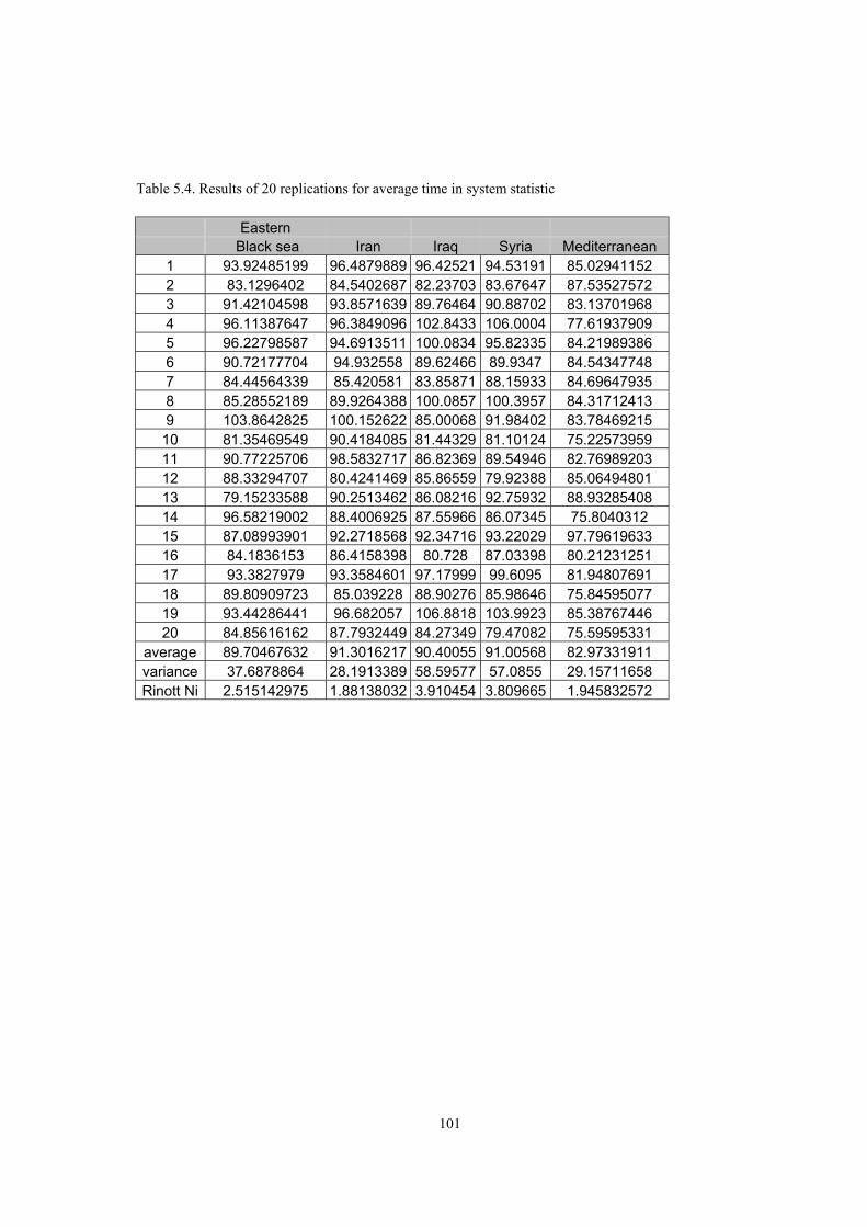
101
Table 5.4. Results of 20 replications for average time in system statistic Eastern Black sea Iran Iraq Syria Mediterranean
1 93.92485199 96.4879889 96.42521 94.53191 85.02941152 2 83.1296402 84.5402687 82.23703 83.67647 87.53527572 3 91.42104598 93.8571639 89.76464 90.88702 83.13701968 4 96.11387647 96.3849096 102.8433 106.0004 77.61937909 5 96.22798587 94.6913511 100.0834 95.82335 84.21989386 6 90.72177704 94.932558 89.62466 89.9347 84.54347748 7 84.44564339 85.420581 83.85871 88.15933 84.69647935 8 85.28552189 89.9264388 100.0857 100.3957 84.31712413 9 103.8642825 100.152622 85.00068 91.98402 83.78469215 10 81.35469549 90.4184085 81.44329 81.10124 75.22573959 11 90.77225706 98.5832717 86.82369 89.54946 82.76989203 12 88.33294707 80.4241469 85.86559 79.92388 85.06494801 13 79.15233588 90.2513462 86.08216 92.75932 88.93285408 14 96.58219002 88.4006925 87.55966 86.07345 75.8040312 15 87.08993901 92.2718568 92.34716 93.22029 97.79619633 16 84.1836153 86.4158398 80.728 87.03398 80.21231251 17 93.3827979 93.3584601 97.17999 99.6095 81.94807691 18 89.80909723 85.039228 88.90276 85.98646 75.84595077 19 93.44286441 96.682057 106.8818 103.9923 85.38767446 20 84.85616162 87.7932449 84.27349 79.47082 75.59595331
average 89.70467632 91.3016217 90.40055 91.00568 82.97331911 variance 37.6878864 28.1913389 58.59577 57.0855 29.15711658 Rinott Ni 2.515142975 1.88138032 3.910454 3.809665 1.945832572

102
Table 5.5. Results of 20 replications for number of damaged vehicles statistic
Middle Trakya Middle Anatolia Greece Bulgaria Aegean Black sea
1 13 26 27 25 13 2 14 22 21 21 15 3 8 21 22 29 10 4 11 28 27 29 11 5 8 21 20 21 7 6 10 29 26 21 14 7 6 28 20 17 13 8 12 18 18 27 19 9 12 26 25 17 13
10 5 35 23 28 10 11 10 17 19 20 11 12 9 19 22 12 12 13 13 31 20 26 14 14 5 13 21 20 11 15 12 21 22 27 9 16 7 25 24 25 9 17 7 21 19 15 9 18 9 16 22 19 12 19 13 34 21 28 11 20 11 24 21 19 18
average 9.75 23.75 22 22.3 12.05 variance 7.881578947 35.25 6.842105 25.27368 8.892105263 Rinott Ni 11.85305491 53.01224 10.2898 38.00893 13.37277881

103
Table 5.6. Results of 20 replications for number of damaged vehicles statistic
Eastern Black sea Iran Iraq Syria Mediterranean
1 26 26 25 25 12 2 18 21 17 20 14 3 27 26 25 26 12 4 24 22 21 20 9 5 22 19 22 23 13 6 18 26 19 23 12 7 19 16 16 17 16 8 20 22 32 22 14 9 19 17 13 20 14
10 23 24 19 20 11 11 19 23 18 21 9 12 21 17 13 19 13 13 20 24 24 31 15 14 26 23 21 17 6 15 22 22 25 22 23 16 19 24 21 23 15 17 22 22 26 26 10 18 22 17 17 16 7 19 23 22 20 26 11 20 24 25 20 14 12
average 21.7 21.9 20.7 21.55 12.4 variance 7.484210526 10.09474 21.37895 16.47105 13.2 Rinott Ni 12.48667763 16.84209 35.6687 27.48035 22.02291667
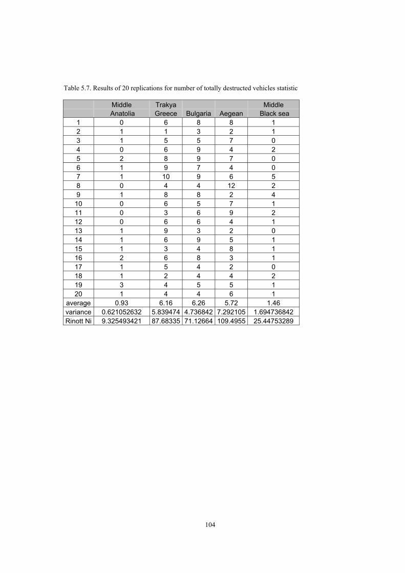
104
Table 5.7. Results of 20 replications for number of totally destructed vehicles statistic
Middle Trakya Middle Anatolia Greece Bulgaria Aegean Black sea
1 0 6 8 8 1 2 1 1 3 2 1 3 1 5 5 7 0 4 0 6 9 4 2 5 2 8 9 7 0 6 1 9 7 4 0 7 1 10 9 6 5 8 0 4 4 12 2 9 1 8 8 2 4 10 0 6 5 7 1 11 0 3 6 9 2 12 0 6 6 4 1 13 1 9 3 2 0 14 1 6 9 5 1 15 1 3 4 8 1 16 2 6 8 3 1 17 1 5 4 2 0 18 1 2 4 4 2 19 3 4 5 5 1 20 1 4 4 6 1
average 0.93 6.16 6.26 5.72 1.46 variance 0.621052632 5.839474 4.736842 7.292105 1.694736842 Rinott Ni 9.325493421 87.68335 71.12664 109.4955 25.44753289

105
Table 5.8. Results of 20 replications for number of totally destructed vehicles statistic Eastern Black sea Iran Iraq Syria Mediterranean
1 5 6 6 7 0 2 2 5 6 4 2 3 6 11 6 6 0 4 7 5 6 9 0 5 10 7 7 5 1 6 1 9 4 6 4 7 8 5 6 7 5 8 8 3 14 6 1 9 5 7 5 7 1 10 5 6 7 8 1 11 5 5 8 5 1 12 7 8 3 9 0 13 8 6 6 6 0 14 7 7 5 6 2 15 11 4 7 6 2 16 6 5 8 6 2 17 5 7 12 3 1 18 6 2 2 6 1 19 5 9 5 7 1 20 9 6 7 7 0
average 5.79 6.32 6.69 6.59 1.16 variance 5.8 4.45 7.315789 2.115789 1.776315789 Rinott Ni 87.090625 66.81953 109.8512 31.7699 26.67249178

106
Table 5.6.1. Number of damaged wheeled trucks by five factors
Middle Trakya Middle Anatolia Greece Bulgaria Aegean Black sea
usual break 3.766 2.433 2.933 2.56 3.4 air attack 1.5 5.566 4.2 4.8 2.83 artillery 0 4.133 4.066 3.7 0 mine 0.3 1.2 1.13 1.466 0.8
ambush 0.4 1.866 1.933 1.933 0.933 total 5.966 15.198 14.262 14.459 7.963
Table 5.6.2. Number of damaged wheeled trucks by five factors
Eastern Black sea Iran Iraq Syria Mediterranean
usual break 2.66 1.66 1.66 1.4 2.93 air attack 4.4 4.8 4.8 4.8 2.53 artillery 3.66 4.4 3.733 4.13 0 mine 1.466 1.46 1.6 1.6 0.933
ambush 1.66 1.66 2.066 2.066 1.2 total 13.846 13.98 13.859 13.996 7.593
Table 5.6.3. Number of damaged armored vehicles by five factors
Middle Trakya Middle Anatolia Greece Bulgaria Aegean Black sea
usual break 2.8 2.133 2.133 2.133 2.133 air attack 0.55 2.2 1.4 1.866 1 artillery 0 2.33 2.33 1.966 0 mine 0.266 0.66 0.6 0.733 0.533
ambush 0.2 1.3 1.3 1.3 0.33 total 3.816 8.623 7.763 7.998 3.996
Table 5.6.4. Number of damaged armored vehicles by five factors
Eastern Black sea Iran Iraq Syria Mediterranean
usual break 2.233 1.533 1.533 1.533 2.133 air attack 1.33 1.8 1.6 1.53 0.8 artillery 2.2 2.66 2 2.33 0 mine 0.733 0.733 0.766 0.766 0.533
ambush 1.3 1.3 1.4 1.4 0.8 total 7.796 8.026 7.299 7.559 4.266

107
Table 5.7.1. Number of totally destructed wheeled trucks by five factors
Middle Trakya Middle Anatolia Greece Bulgaria Aegean Black sea
usual break 0.166 0 0.066 0 0 air attack 0.3 1 1 0.666 0.333 artillery 0 2.766 2.8 2.4 0 mine 0.166 0.4 0.533 0.866 0.466
ambush 0.066 0.4 0.266 0.266 0.33 total 0.698 4.466 4.665 4.198 1.129
Table 5.7.2. Number of totally destructed wheeled trucks by five factors
Eastern Black sea Iran Iraq Syria Mediterranean
usual break 0.133 0 0.066 0 0 air attack 0.666 0.866 1 0.66 0.33 artillery 2.2 2.53 2.466 2.8 0 mine 0.8 0.8 0.733 1.2 0.6
ambush 0.333 0.133 0.466 0.2 0.133 total 4.132 4.329 4.731 4.86 1.063
Table 5.7.3. Number of totally destructed armored vehicles by five factors
Middle Trakya Middle Anatolia Greece Bulgaria Aegean Black sea
usual break 0.066 0 0 0 0 air attack 0.066 0.266 0.066 0.2 0.133 artillery 0 1.13 1.33 1.13 0 mine 0 0 0 0 0
ambush 0.1 0.2 0.2 0.2 0.2 total 0.232 1.596 1.596 1.53 0.333
Table 5.7.4. Number of totally destructed armored vehicles by five factors
Eastern Black sea Iran Iraq Syria Mediterranean
usual break 0 0 0 0 0 air attack 0.133 0.133 0.2 0.133 0 artillery 1.33 1.46 1.266 1.4 0 mine 0 0 0 0 0
ambush 0.2 0.4 0.5 0.2 0.1 total 1.663 1.993 1.966 1.733 0.1

108
APPENDIX D A PART OF CODE OF THE SIMULATION MODEL (MODEL FRAME) 0$ BEGIN, Yes,headquarters wheel; 1$ CREATE, 75:,1; 2$ ASSIGN: VSayac4=VSayac4+1: Truckno4=VSayac4: company#=4; 3$ STATION, Enter4; 17$ BRANCH, 1: If,Truckno4<2,muh,Yes: Else,ORD,Yes; muh ASSIGN: VBROKE20=DISC(0.02,0,1,1,36); 232$ BRANCH, 1: If,VBROKE20==0,pull42,Yes: Else,yukle42,Yes; pull42 COUNT: garagebreak42,1; 5$ DELAY: TRIA(8,12,16); take on vehicle yukle42 QUEUE, Vehicle42Q; 4$ REQUEST, 1:Vehicle42(SDS),430,Enter4; 6$ TRANSPORT: Vehicle42,AMMO,430; ORD ASSIGN: VBROKE21=DISC(0.02,0,1,1,36); 230$ BRANCH, 1: If,VBROKE21==0,pull41,Yes: Else,yukle41,Yes; pull41 COUNT: garagebreak41,1; 231$ DELAY: TRIA(8,12,16); yukle41 DELAY: TRIA(8,10,12); Garage storage loading 7$ QUEUE, Vehicle41Q; 8$ REQUEST, 1:Vehicle41(SDS),430; 9$ TRANSPORT: Vehicle41,sayac,430; 14$ STATION, AITB4; 15$ DELAY: 0; 16$ TALLY: time in system4,INT(VArrTime1),1; bak BRANCH, 1: If,maingroup==102,dev,Yes: Else,vdur,Yes; dev BRANCH, 1: If,Vtruck1#==3,emir2,Yes: If,Vtruck2#==3,emir3,Yes: If,Vtruck3#==3,emir4,Yes: If,Vtruck4#==3,emir5,Yes: Else,vscenario,Yes; emir2 DELAY: 30; harekat emri 59$ DELAY: 0; take on

109
111$ ASSIGN: left=left+1; 247$ TALLY: check,INT(VArrTime1),1; 110$ SIGNAL: 102,102; vscenario TRANSPORT: ,Vcheck1,430; emir3 DELAY: 33:NEXT(59$); emir4 DELAY: 36:NEXT(59$); emir5 DELAY: 39:NEXT(59$); vdur WAIT: 75,102:NEXT(dev); 18$ STATION, Gaitb4; 19$ TALLY: VGiris4,INT(VArrTime1),1; 33$ ASSIGN: Vsayac5=Vsayac5+1: Vtruck4#=Vsayac5; 20$ TRANSPORT: ,AITB4,430; 22$ CREATE, 9:,1:MARK(VArrTime1); tank company wheel 107$ ASSIGN: company#=1; 23$ STATION, Enter1; 234$ BRANCH, 1: With,0.02,pull1,Yes: Else,yukle1,Yes; pull1 COUNT: garagebreak1,1; 233$ DELAY: TRIA(8,12,16); yukle1 DELAY: TRIA(8,10,12); garage depot loading 24$ QUEUE, Vehicle1Q; 25$ REQUEST, 1:Vehicle1(SDS),430,Enter1; 26$ TRANSPORT: Vehicle1,sayac,430; 27$ STATION, AITB1; 28$ DELAY: 0; get off 29$ TALLY: Time in system1,INT(VArrTime1),1; 34$ ASSIGN: varisno1=varisno1+1: Vtruck1#=varisno1:NEXT(bak); 30$ STATION, GAITB1; 31$ TALLY: VGiris1,INT(VArrTime1),1; 32$ TRANSPORT: Vehicle1,AITB1,430; 35$ STATION, AMMO:MARK(ammo1); 10$ DELAY: UNIFORM(0.5,1); take off 11$ DELAY: TRIA(8,10,12); loading 12$ DELAY: UNIFORM(2,3); take on 36$ TALLY: loadertime,INT(ammo1),1; 13$ TRANSPORT: Vehicle42,sayac,430; 37$ CREATE, 9:,1; tank company wheel2 108$ ASSIGN: company#=2; START2 STATION, Enter2; 235$ BRANCH, 1: With,0.02,pull2,Yes: Else,yukle2,Yes; pull2 COUNT: garagebreak2,1;

110
APPENDIX E PROBABILITY TREE OF WHEELED-TRUCKS
With 0.02 probability 20 minutes tdv : totally destructed vehicle
Alert order
0.45 20 0.94
con’t 0.35 35
0.19 50
0.01 tdv
0.06 breakdown
0.02 12+10
0.98 10
30
1
0.02 20
111
PROBABILITY TREE OF WHEELED-TRUCKS (cont’d)
With 0.02 probability 20 minutes tdv : totally destructed vehicle
2
0.35 con’t
0.12 45
air attack
0.90 con’t
0.10 0.65
0.18 tdv
0.3 60
0.40 40
artillery
0.92 con’t
0.08 1.5 min
0.50
0.50 con’t
0.60 tdv
0.15 60
0.15 45
0.10 30
1
0.02 20
112
PROBABILITY TREE OF WHEELED-TRUCKS (cont’d)
With 0.02 probability 20 minutes tdv : totally destructed vehicle
2 Mine
0.98 con’t
0.02 1,5+10
0.28 con’t
0.72
0.50 tdv
0.20 80
0.20 60
0.10 30
ambush
0.96 con’t
0.04
0.30 con’t
0.70
0.20 con’t
0.80
0.18 tdv
0.20 60
0.20 45
0.42 30
0.02 20

113
PROBABILITY TREE OF ARMORED VEHICLES
With 0.02 probability 20 minutes tdv : totally destructed vehicle
Alert order
0.15 20 0.94
con’t 0.55 35
0.29 50
0.01 tdv
0.06 breakdown
0.01 12+15
0.98 12
30
1
0.02 20

114
PROBABILITY TREE OF ARMORED VEHICLES (cont’d)
With 0.02 probability 20 minutes tdv : totally destructed vehicle
2
0.45 con’t
0.33 60
air attack
0.90 con’t
0.10 0.55
0.07 tdv
0.35 45
0.45 30
artillery
0.88 con’t
0.12 1.5 min
0.35
0.65 con’t
0.57 tdv
0.08 60
0.15 45
0.20 30
1
0.02 20

115
PROBABILITY TREE OF ARMORED VEHICLES (cont’d)
With 0.02 probability 20 minutes tdv : totally destructed vehicle
2 Mine
0.96 con’t
0.04 10
0.73 con’t
0.27
0.33 tdv
0.30 80
0.21 60
0.16 30
ambush
0.94 con’t
0.06
0.45 con’t
0.55
0.45 con’t
0.55
0.27 tdv
0.20 60
0.20 45
0.33 30
0.02 20
BIBLIOGRAPHY Alexopoulos, C. and A. F. Seila. (1998). “Advanced methods for simulation output
analysis”. Proceedings of the 1998 Winter Simulation Conference. pp. 113-120.
Allen, P. D. and B. A. Wilson. (1988). “Modeling qualitative issues in military
simulations with the RAND-ABEL language”. Proceedings of the 1988 Winter
Simulation Conference. pp. 372-380.
Balci, O. (1998). “Verification, validation, and accreditation”. Proceedings of the 1998
Winter Simulation Conference. pp. 42-48.
Banks, J., S. Carson II and B. L. Nelson. (1996). Discrete Event System Simulation.
Prentice-Hall, Inc. , New Jersey.
Banks, J. (1998). Handbook of simulation, John Wiley & Sons, Inc.,.Newyork.
Blais, C. L. (1994). “Marine Air Ground Task Force (MAGTF) Tactical Warfare
Simulation (MTWS)”. Proceedings of the 1994 Winter Simulation Conference. pp. 839-
844.
Blais, C. L. (1995). “Scalability Issues in enhancement of the MAGTF Tactical Warfare
Simulation System”. Proceedings of the 1995 Winter Simulation Conference. pp. 1280-
1287.
Caldwell, W. J. , R. Wood and M. C. Pate. (1995). “JLINK-JANUS fast movers”.
Proceedings of the 1995 Winter Simulation Conference. pp. 1237-1245.
Centeno, M.A. and Reyes, M.F. (1998). “ So you have model. What to do next, a
tutorial on simulation output analysis”. Proceedings of the 1998 Winter Simulation
Conference. pp. 23-29.
116

Childs, C. and T. Lubaczewski. (1987). “A battalion/brigade training simulation”.
Proceedings of the 1987 Winter Simulation Conference. pp. 876-883.
Department of the Army Pamphlet 5-11. (1999). Verification, Validation, and
Accreditation of Army Models and Simulations. Headquarters Department of the Army
Washington, DC.
Department of the Army. (1996). “Mobilization and Deployment”. FM 71-3 The
Armored and Mechanized Infantry Brigade. pp. 120-124.
Garrabbrants, W. M. (1998). “Simulation as a mission planning and rehearsal tool” .
Proceedings of the 1998 Winter Simulation Conference. pp. 849-853.
Garrambone, M. W. (1992). “An overview of air land combat modeling and simulation”.
Proceedings of the 1992 Winter Simulation Conference. pp. 1130-1138.
Hatley, D.S. (1997). “Verification and validation in military simulations”. Proceedings
of the 1997 Winter Simulation Conference. pp. 925-932.
Henry, H. (1994). “The Corps Battle Simulation: remodeling the model for new
missions”. Proceedings of the 1994 Winter Simulation Conference. pp. 788-791.
Johnson, W. R., T. W. Mastaglio and P. D. Peterson. (1993). “The Close Combat
Tactical Trainer Program”. Proceedings of the 1993 Winter Simulation Conference. pp.
1021-1030.
Genel Kurmay Başkanlığı Kara Kuvvetleri Komutanlığı. (1994). Turkish Army Logistic
Procedures (KKY 54-5)., Ankara.
Kathman, R. (1995). “Data collection in field combat simulation”. Proceedings of the
1985 Winter Simulation Conference. pp. 376-380.
117
Kelton , W.D., and A. M. Law. (1991). Simulation Modeling Analysis. McGraw-Hill,
inc.
Kelton, W.D. (1997). “Statistical analysis of simulation output”. Proceedings of the 1997
Winter Simulation Conference. pp. 23-30.
Kleijnen, J.P.C. 1999. Validation of models: Statistical techniques and data availability. .
Proceedings of the 1999 Winter Simulation Conference, 647-654.
Montgomery, D. C. (1984). Design and Analysis of Experiments. John Wiley & Sons,
Inc.
Oswalt, I. (1995). “Technology trends in military simulation”. Proceedings of the 1995
Winter Simulation Conference. pp.1152-1157.
Page, E. H. and R. Smith. (1998). “Introduction to military training simulation: A guide
for discrete event simulationists”. Proceedings of the 1998 Winter Simulation
Conference. pp. 53-60.
Painter, R. D. (1995). “Object-oriented military simulation development and
application”. Proceedings of the 1995 Winter Simulation Conference. pp. 1185-1192.
Parker, S. R. (1995). “Military force structure and realignment “ sharpening the edge”
through the dynamic simulation”. Proceedings of the 1995 Winter Simulation
Conference. pp. 1288-1296.
Parker, S. R. (1991). “Combat vehicle reliability assessment simulation model
(CVRASM)”. Proceedings of the 1991 Winter Simulation Conference. pp. 491-498.
Proctor, M. D. and J. C. Gubler. (1998). “Military simulation worlds and organizational
learning”. Proceedings of the 1998 Winter Simulation Conference. pp.773-778.
118

Rinott, Y. (1978). Communications in Statistics-Theory and Methods.
Roland, R.J. (1998). “Panel: The future of military simulation”. Proceedings of the 1998
Winter Simulation Conference. pp. 813-817.
Russell, D. B. and W. K. McQuay. (1993). “The joint modeling and simulation system: a
common modeling architecture for DoD”. Proceedings of the 1993 Winter Simulation
Conference. pp. 984-988
Sanchez, S. M. (1999). “ABC’s of output analysis”. Proceedings of the 1999 Winter
Simulation Conference. pp. 24-32.
Sargent, R.G. (1998). “Verification and validation of simulation models”. Proceedings of
the 1998 Winter Simulation Conference. pp.121-130.
Sisti, A.F. (1996). “Modeling and simulation technologies for military applications”.
Proceedings of the 1996 Winter Simulation Conference. pp. 877-883.
Smith, R.D. (1998). “Essential techniques for military modeling and simulation”.
Proceedings of the 1998 Winter Simulation Conference. pp. 805-812.
Takus, D.A. and D.M. Profozich. (1997). “ARENA software tutorial”. Proceedings of
the 1997 Winter Simulation Conference. pp. 541-544.
Winston, W.L. (1994). Operations Research, Duxbury Press.
Youngren, M.A., S. H. Parry, D. P. Gaver and P. A. Jacobs. (1994). “The Future
Theater-Level Model: a research project update”. Proceedings of the 1994 Winter
Simulation Conference. pp. 829-834.
119