EVALUATION OF FUNDAMENTAL ORGANIC … OF FUNDAMENTAL ORGANIC CONCEPTS by MATTHEW DAVISSON WODRICH...

EVALUATION OF FUNDAMENTAL ORGANIC CONCEPTS

by

MATTHEW DAVISSON WODRICH

(Under the Direction of Paul von Ragué Schleyer)

ABSTRACT

The concept of protobranching, defined as the net stabilization provided by 1,3-alkyl-

alkyl interactions in all branched and n-alkanes except methane and ethane, and its

implications are highlighted. Protobranching is assessed via Pople’s isodesmic bond

separation energy and has an average value of 2.8 kcal/mol for n-alkanes. Protobranching

has a significant impact on the quantification of physical organic phenomena, including

ring/cage strain, conjugation and hyperconjugation, and aromatic resonance energies.

Historically, these quantities have been evaluated using propane and larger alkanes (both

linear and branched) as reference compounds. However, the inherent stabilization within

these “reference” compounds has not previously been considered. Reevaluated energies

for the above mentioned phenomena are discussed. Protobranching has also been utilized

to create a new isodesmic additivity scheme, capable of calculating heats of formation of

alkanes, alkyl radicals, alkenes, and alkynes to high accuracy. Data fitting schemes based

on geminal interactions are also explored. The ability of computational methods (HF,

DFT, and post-HF) to compute the magnitude of protobranching stabilization is

investigated. Pople’s isodesmic bond separation reactions of n-alkanes (propane to

decane) show systematic underestimation for all DFT functionals tested; they are unable

to accurately account for the protobranching stabilization. In the final chapter, double

aromaticity, the existence of two mutually orthogonal Hückel frameworks within the

same molecule, of small carbon, boron, and borocarbon monocycles is analyzed using

refined NICS techniques. Double aromaticity is confirmed in C6 and C10, as had been

previously hypothesized. C8 and C12 are shown to be doubly antiaromatic. Select boron

and borocarbon compounds are also shown to be doubly aromatic.

INDEX WORDS: COMPUTATIONAL CHEMISTRY, DENSITY FUNCTIONAL

THEORY, PROTOBRANCHING, CONJUGATION, HYPERCONJUGATION,

RESONANCE ENERGY, AROMATIC STABILIZATION ENERGY,

AROMATICITY, DOUBLE AROMATICITY, BOROCARBON, ISODESMIC,

HOMODESMOTIC, BOND SEPARATION ENERGY, ADDITIVITY SCHEME,

HYDROCARBON


by


B.S., The University of Arizona, 2002

B.A., The University of Arizona, 2002

A Dissertation Submitted to the Graduate Faculty of The University of Georgia in Partial

Fulfillment of the Requirements for the Degree

DOCTOR OF PHILOSOPHY

ATHENS, GEORGIA

2006

! 2006

Matthew Davisson Wodrich

All Rights Reserved


by


Major Professor: Paul von Ragué Schleyer

Committee: Henry F. Schaefer III

Robert J. Woods

Electronic Version Approved:

Maureen Grosso

Dean of the Graduate School

The University of Georgia

December 2006

iv

DEDICATION

For my parents Dave and Sue Wodrich, because, “everyone gets a Ph.D.”

v

ACKNOWLEDGMENT

So many people have had an impact on both my personal and professional life, and have

played important roles in allowing me to achieve what I have. Early on, Mr. Ed Eberle

(Dobson High School) and Dr. Robert Mangham (Arizona State University) had

enormous influence and helped steer me toward the sciences. Dr. Ana Moore, an

absolutely fabulous teacher instilled the basics of organic chemistry in me. Every time I

here the word “carbocation” my thoughts go back to her organic class. From the

University of Arizona I have to thank my undergraduate chemistry advisor and physical

chemistry teacher Dr. Walter Miller. It was Dr. Miller that encouraged me to apply to

UGA for my graduate studies. Also of tremendous influence was Dr. Dan Liebler of the

UA College of Pharmacy. Dr. Liebler allowed me to work in his lab for my required

senior thesis. Although I ultimately did not end up studying chemical toxicology, the

subject of my senior thesis, the skills I learned during that year have helped me

tremendously during my Ph.D. studies.

UGA has provided an excellent and fostering environment for my Ph.D. First I

have to thank the people I have worked with on a day-to-day basis for the past four years.

Dr. Chait Wannere, was always willing to help, particularly during my first year when we

shared an office. He showed me how to submit jobs, and how to view orbitals, certainly

important things for a computational chemistry. Several other graduate students joined

the Schleyer group after me; Debjani, Keigo, and Judy. Although I have had a relatively

small amount of direct work with them, we have always gotten along well and have been

there for each other to discuss things in general or complain about the problems of the

day. Finally the postdocs that have helped during my stay, Dr. Sung Soo Park, Dr.

vi

Zhongfang Chen, and Dr. Clémence Corminboeuf. All of you have provided a wonderful

and fostering work environment. Only on rare occasion was a question to stupid to ask in

your presence. Clemi the amount of time you have taken out of your schedule to read my

papers, figure out why my job wasn’t working, getting a new script to run correctly, and

probably about a million other little things has not gone unappreciated. Your scientific

and work focused mind set should be an example to all aspiring graduate students.

Several professors have played very important roles. Dr. R. Bruce King, Dr. Henry

Schaefer and Dr. Robert Woods deserve special recognition, having been extremely

helpful and patient serving as members of my committee. I also point out that Dr.

Schaefer has provided a wonderful work environment here in Center for Computational

Chemistry. I’d also like to thank Dr. Lou Allinger, for many friendly discussions on

various aspects of organic chemistry. Last and certainly not least is Dr. Paul Schleyer,

who has been the key factor in helping me acquire and understand nearly all of the

chemical knowledge I have today. Your friendly chats and harsh questioning sessions

have helped me greatly. Your writing style is unmatched in the literature, and should be

the model for which all scientist writing papers should follow. I hope that the tremendous

love for all things scientific you have has been passed on, at least in part, to me.

Countless others have helped me out, not directly in my work, but behind the

scenes. Most importantly have been my parents, Dave and Sue, to whom this dissertation

is dedicated. I hope you feel that the years of paying for college you have paid for haven’t

been a waste. I couldn’t have done any of this without your constant support. My sister

Jill needs special thanking as well, you’ve always been willing to entertain me when I

was getting tired of working or just needed to talk to someone. I hope that you’ve felt the

vii

same way about me (especially with your own thesis defense coming up). Numerous

friends have helped along the way, most notably has been Justin Turney, who introduced

me to the field of computational chemistry and encouraged me to consider choosing Dr.

Schleyer as a research advisor. We have spent countless hours together during the past

four years. Lunch and dinner every day during first semester, all those homework

assignments, and just hanging out watching a football game or movie have been great.

The DePalma’s Thursday lunch has been one of my favorite graduate school traditions,

and I will sorely miss it when I leave this place. My friends back home need special

mentioning also, Will, Ivan, Ben, and Vancifer (like Lucifer, only Vancifer), I want to

thank you for all your support.

To someone special: Je t’aime ma Swissy.

viii

TABLE OF CONTENTS

Page

ACKNOWLEGMENTS..................................................................................................v

LIST OF TABLES ..........................................................................................................x

LIST OF SCHEMES.....................................................................................................xv

LIST OF FIGURES......................................................................................................xvi

CHAPTER

1 INTRODUCTION, BACKGROUND, AND CHAPTER SUMMARY.......1

1.1 PREAMBLE ........................................................................................2

1.2 HARTREE-FOCK THEORY...............................................................3

1.3 POST HARTREE-FOCK METHODS..................................................5

1.4 DENSITY FUNCTIONAL THEORY ..................................................5

1.5 CHAPTER SUMMARY ....................................................................11

1.6 REFERENCES...................................................................................13

2 THE CONCEPT OF PROTOBRANCHING AND ITS MANY

PARADIGM SHIFTING IMPLICATIONS FOR ENERGY

EVALUATIONS .....................................................................................16

2.1 ABSTRACT.......................................................................................17

2.2 INTRODUCTION..............................................................................18

2.3 RESULTS AND DICUSSION ...........................................................25

2.4 CONCLUSIONS................................................................................57

2.5 ACKNOWLEDGMENTS ..................................................................59

ix

2.6 REFERENCES...................................................................................60

3 NEW ADDITIVITY SCHEMES FOR HYDROCARBON ENERGIES...................67

3.1 ABSTRACT.......................................................................................68

3.2 INTRODUCTION..............................................................................68

3.3 BRANCHING AND ATTENUATION ..............................................76

3.4 HYPERCONJUGATION IN ALKENES, ALKYNES, AND ALKYL

RADICALS........................................................................................76

3.5 METHOD OF APPLICATION ..........................................................77

3.6 CYCLIC MOLECULES.....................................................................77

3.7 ACKNOWLEDGMENTS ..................................................................78

3.8 SUPPORTING INFORMATION .......................................................80

3.9 REFERENCES................................................................................. 101

4 SYSTEMATIC ERRORS IN COMPUTED ALKANE ENERGIES USING B3LYP

AND OTHER POPULAR DFT FUNCTIONALS.................................................. 102

4.1 ABSTRACT..................................................................................... 103

4.2 INTRODUCTION............................................................................ 103

4.3 METHODS ...................................................................................... 105

4.4 RESULTS AND DISCUSSION ....................................................... 106

4.5 ACKNOWLEDGMENTS ................................................................ 111

4.6 REFERENCES................................................................................. 112

5 AROMATCITY AND DOUBLE AROMATICITY IN MONOCYCLIC BORON,

CARBON, AND BOROCARBON COMPOUNDS............................................... 119

5.1 ABSTRACT..................................................................................... 120

x

5.2 INTRODUCTION............................................................................ 120

5.3 METHODS ...................................................................................... 125

5.4 RESULTS AND DISCUSSION ....................................................... 128

5.5 CONCLUSIONS.............................................................................. 145

5.6 ACKNOWLEDGMENTS ................................................................ 146

5.7 REFERENCES................................................................................. 148

6 CONCLUSION ..................................................................................................... 159

7 LIST OF PUBLICATIONS ................................................................................... 162

xi

LIST OF TABLES

Page

TABLE 2.1: Evaluation of bond separation energies for saturated hydrocarbons (in

kcal/mol). NIST 298K thermochemical data were employed .....................26

TABLE 2.2: Performance of various theoretical levels in evaluating branching

stabilization. The 6-311++G(d,p) basis set was used throughout. E0 is the

quantity given by the electronic energies. ZPE/Thermal is the contribution to

branching stabilization from scaled zero-point vibrational and thermal

corrections to 298K. ..................................................................................30

TABLE 2.3: Benson group increments for 298K alkanes and values expected on the basis

of a regular progression. Differences between Benson and expected values

are used to evaluate protobranching. All data in kcal/mol. .........................31

TABLE 2.4: Strain energies of cyclopropane based on the BSE Equation 11. E0 (the

electronic) and ZPE/Thermal energies (the scaled zero-point and thermal

corrections to 298K) are in kcal/mol. The 6-311++G(d,p) basis set was

employed uniformly. .................................................................................37

TABLE 2.5: Cyclobutane BSE evaluations of Equation 13 (in kcal/mol). E0 is the

electronic energy. ZPE/Thermal is the scaled zero-point vibrational and

thermal corrections to 298K. .....................................................................38

TABLE 2.6: BSE evaluations of Equations 17, 20, 22, 24, 27 and 28 (in kcal/mol). E0 is

the electronic energy. ZPE/Thermal is the scaled zero-point vibrational and

thermal corrections to 298K. .....................................................................43

xii

TABLE 2.7: BSE analysis of propene. The E0 (electronic) and the ZPE/Thermal (scaled

zero-point vibrational and thermal corrections to 298K) are in kcal/mol. All

computations used the 6-311++G(d,p) basis set. ........................................46

TABLE 2.8: Evaluation of bond separation energies for unsaturated hydrocarbons (in

kcal/mol). NIST thermochemical data at 298K were employed..................50

TABLE 2.9: Summary of conventional, revised, and BLW (at HF and B3LYP) energy

evaluations of strain, hyperconjugation, conjugation, and benzene

aromaticity (kcal/mol) ...............................................................................59

TABLE 3.1: Heats of formation of Gronert’s strain–free hydrocarbons as well as alkynes,

in kcal/mol. Molecules shown in bold font were used to derive the isodesmic

parameters and attenuation coefficients employed in Scheme 3.2 and Table

3.2.............................................................................................................69

TABLE 3.2: Parameters employed in Scheme 3.2. Experimental !Hf data (in kcal/mol)

were used for their evaluation....................................................................75

TABLE 3.3: Table used to derive values for heats of formation using the isodesmic

additivity scheme. The number in each column represents the number of

each specific interaction present in the molecule of interest. This number is

then multiplied by the value for the interaction located at the top of each

column. The value of the summed interactions is then subtracted from the

base value, giving !Hf. All values in kcal/mol. .........................................80

TABLE 3.4: Summary of values (in kcal/mol) from Tables 3.5-3.19. Fixed parameters

are given in red; experimental data are in bold font. The value Gronert used

xiii

are in italics. Parameters in black were free to vary. Data fitting were done

using Excel................................................................................................85

TABLE 3.5: Gronert’s scheme. Average deviation is 0.22 kcal/mol...............................86

TABLE 3.6: Scheme where C = 231.3 and H =52.1, all other parameters free to vary.

Average deviation is 0.19 kcal/mol............................................................87

TABLE 3.7: Scheme where H=52.1, all other parameters free to vary. Average deviation

is 0.18 kcal/mol. ........................................................................................88

TABLE 3.8: No fixed parameters. Average deviation is 0.18 kcal/mol. .........................89

TABLE 3.9: Scheme where H=52.1, C=200.0, all other parameters free to vary. Average

deviation is 1.02 kcal/mol..........................................................................90

TABLE 3.10: Scheme where C = 170.6 and H = 52.1, all other parameters free to vary.

Average deviation is 1.84 kcal/mol.........................................................91

TABLE 3.11: Scheme using 2CH and 3CH2 and no fixed parameters. Average deviation is

0.40 kcal/mol..........................................................................................92

TABLE 3.12: Scheme using 2CH and 3CH2, C=170.6, H=52.1, all other parameters free to

vary. Average deviation is 1.12 kcal/mol. ...............................................93

TABLE 3.13: Scheme with no CH, and no fixed parameters. Average deviation is 0.24

kcal/mol. ................................................................................................94

TABLE 3.14: Scheme with no CH, C=200.0, and H=52.1, all other parameters free to


TABLE 3.15: Scheme with no CH, C=170.6, and H=52.1, all other parameters free to


xiv

TABLE 3.16: Scheme where CH and 3CH2 have been removed, all other parameters free

to vary. Average deviation is 0.19 kcal/mol. ...........................................97

TABLE 3.17: Scheme with CH and 3CH2 removed, H = 52.1, all other parameters free to


TABLE 3.18: Scheme with CH and 3CH2 removed, C = 170.6 and H = 52.1, all other

parameters free to vary. Average deviation is 0.19 kcal/mol. ..................99

TABLE 3.19: Scheme with CH and 3CH2 removed, C = 170.6, H = 52.1, CCH = 0.0,

CCC = 0.0, all other parameters free to vary. Average deviation is 0.50

kcal/mol. .............................................................................................. 100

TABLE 5.1: Point groups, NICS, and dissected CMO-NICS for relevant compounds.. 147

xv

LIST OF SCHEMES

Page

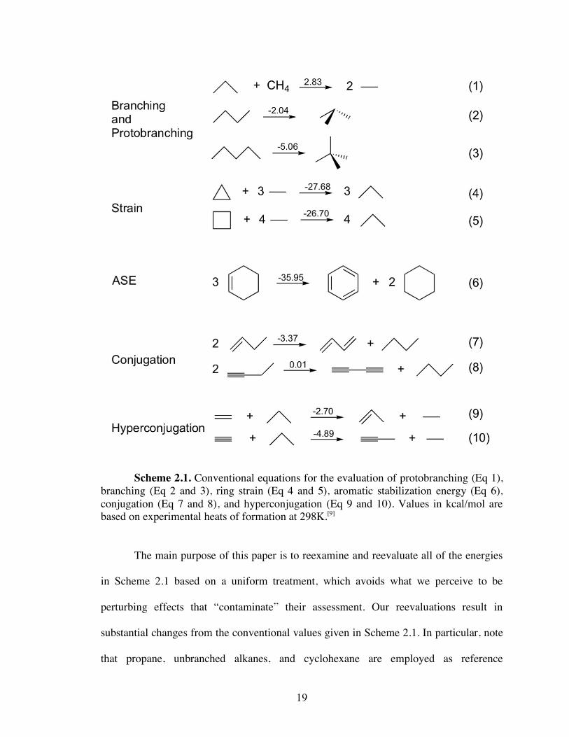
SCHEME 2.1: Conventional equations for the evaluation of protobranching (Eq 1),

branching (Eq 2 and 3), ring strain (Eq 4 and 5), aromatic stabilization

energy (Eq 6), conjugation (Eq 7 and 8), and hyperconjugation (Eq 9 and

10). Values in kcal/mol are based on experimental heats of formation at

298K.....................................................................................................19

SCHEME 2.2: Equations that have been employed to evaluate the resonance energy of

benzene. The upper values are the original RE estimates. The lower

values are the RE’s after correction for the perturbing effects of

protobranching, hyperconjugation, and conjugation. .............................53

SCHEME 2.3: Equations used to evaluate aromatic stabilization energy of benzene. .....56

SCHEME 3.1: (a) Gronert’s method for evaluating alkane, cycloalkane, alkene, and alkyl

radical heats of formation. (b) Four-parameter simplification employing

experimental H and C data. (See Tables 3.5 and 3.19.)..........................71

SCHEME 3.2: Generalized isodesmic method for calculating heats of formation of

unstrained alkanes, alkenes, alkynes, and alkyl radicals (in kcal/mol). See

the text and the parameters in Table 3.2 for details of the applications and

the evaluations. .....................................................................................73

xvi

LIST OF FIGURES

Page

FIGURE 2.1: Protobranching interactions in propane (1), n-butane (2), and isobutane (3).

Similarly, neopentane and cyclohexane have six protobranching

interactions each. While branched alkanes have a greater number of

protobranches, attractive 1,3-alkyl-alkyl interactions also are present in

linear alkanes. ........................................................................................21

FIGURE 2.2: Benson group increment values and protobranching corrected group

increment values.....................................................................................32

FIGURE 2.3: Baeyer (angle) ring strain for planar (SiH2)n rings as computed by the BSE

equation n Si2H6 " n SiH4 + (SiH2)n. Si-H bonds are partially ionic and

silicon does not rehybridize when the ring bond angles are deformed.

Hence, the strain of small silicon rings follows Baeyer’s expectation......35

FIGURE 2.4: Baeyer ring strain for planar (CH2)n rings, as computed by the BSE

equation, n C2H6 " n CH4 + (CH2)n. Note the marked deviation of

cyclopropane from Baeyer’s expectations and from the behavior of

trisilacyclopropane (Figure 2.3).. ............................................................36

FIGURE 2.5: Comparison plots (derived from George et al.), based on experimental data)

of the strain energies (in kcal/mol) given by the homodesmotic (Equation

14, blue points) and isodesmic reactions (Equation 15, red points), as a

function of cycloalkane ring size. ...........................................................39

FIGURE 2.6: Original values and stabilization revised values for aromatic stabilization

energies calculated by various equations (Scheme 2.2). ..........................55

xvii

FIGURE 3.1: Performance of our new isodesmic additivity scheme. .............................79

FIGURE 4.1: Error per bond in calculated enthalpies of formation for n-alkanes.

Reproduced from Reference 4 .............................................................. 104

FIGURE 4.2: Deviations of various DFT functionals from experimental (0 K)

protobranching stabilization energies. Negative values denote

underestimation. Stabilization energies are based on Equation 1. CCSD(T)

and MP2 refer to CCSD(T)/aug-cc-pVTZ//MP2/6-311+G(d,p) and

MP2/aug-cc-pVTZ//MP2/6-311+G(d,p), respectively, and include MP2/6-

311+G(d,p) zero-point corrections. All other computations employed the

6-311+G(d,p) basis set.......................................................................... 106

FIGURE 5.1: The planar C6H3+ doubly aromatic ion comprised of 6! electrons and 2

radial in-plane electrons........................................................................ 121

FIGURE 5.2: Double aromatic structures of C10H5- (10! + 6 rad) and

C8H4 (10! + 2 rad)................................................................................ 121

FIGURE 5.3: Double aromatic structures proposed by Hofmann and Berndt. Reproduced

from Reference 110 and neutral CB2..................................................... 125

FIGURE 5.4: Geometries, point groups, and isotropic NICS values (red indicates

diatropicity while green indicated paratropicity) of carbon clusters....... 130

FIGURE 5.5: CMO-NICS plot of C6H3+. CMO-NICS and CMO-NICSzz contributions are

listed on the right side in ppm; the “Total” listed at the bottom represents

the contributions of all orbitals, not just those pictured. MO energies in

a.u. are given on the left side. ............................................................... 131

xviii

FIGURE 5.6: NICS!zz and NICSradzz grids of C6 (D3h and D6h). The NICS

!zz grids indicate

the ! systems to be diatropic within the molecular framework while the

NICSradzz grids indicates the radial system is paratropic in the central

triangle and diatropic in the outer triangles for D3h and diatropic

throughout for D6h. ............................................................................... 133

FIGURE 5.7: Proposed ring current model for the radial system of D3h C6. .................. 134

FIGURE 5.8: D6h (A) and D3h (B) CMO-NICS plots of C6. CMO-NICS and CMO-NICSzz

contributions are listed on the right side in ppm; the “Total” listed at the

bottom represents the contributions of all orbitals, not just those pictured.

MO energies in a.u. are given on the left side. ...................................... 135

FIGURE 5.9: B3LYP/6-311+G(d) optimized bond angles of polyallene D5h C10 and D7h

C14. ....................................................................................................... 136

FIGURE 5.10: CMO-NICS and CMO-NICSzz of doubly anti-aromatic C8. CMO-NICS

and CMO-NICSzz contributions are listed on the right side in ppm; the

“Total” listed at the bottom represents the contributions of all orbitals,

not just those pictured. MO energies in a.u. are given on the left side.. 138

FIGURE 5.11: CMO-NICS and CMO-NICSzz of doubly antiaromatic C12. CMO-NICS

and CMO-NICSzz contributions are listed on the right side in ppm; the

“Total” listed at the bottom represents the contributions of all orbitals,

not just those pictured. MO energies in a.u. are given on the left side.. 139

FIGURE 5.12: Mixed aromatic/antiaromatic systems reported by Hofmann and

Berndt................................................................................................. 140

xix

FIGURE 5.13: Geometries, point groups, and isotropic NICS values (red signifies

diatropic) of various rings ................................................................... 142

FIGURE 5.14: CMO-NICS and CMO-NICSzz from canonical molecular orbitals of C4B4.

CMO-NICS and CMO-NICSzz contributions are listed on the right side in

ppm; the “Total” listed at the bottom represents the contributions of all

orbitals, not just those pictured. MO energies in a.u. are given on the left

side ..................................................................................................... 143

CHAPTER 1

INTRODUCTION AND LITERATURE REVIEW

2

1.1 PREAMBLE

Chemists have long been interested in the determination of fundamental molecular

properties, including molecular strain, aromatic resonance energy, and other stabilizing or

destabilizing energetic effects. Typically, such effects cannot be measured directly by

experiment, for example no instrument can tell you the resonance energy of benzene or

the ring strain of cyclopropane. Such energies must be determined using alternate

techniques. Generally, chemical equations are written, which compare the feature of

interest to various “reference” compounds. Using the relevant heats of formation (or

computed energies) a numeric value for the phenomena in question can be obtained.

Clearly, numerous equations could be written, the result being a wide range of values.

The problem lies in the choice of “reference” compounds, which ideally contain minimal

perturbing effects. The importance of these choices is highlighted in this dissertation.

In addition to making use of available thermochemical data, computations are also of

significant importance. The use of computations within the chemistry community has

grown drastically over the past decade. This enhancement has been fueled by notable

increases in computer speed, reduction in cost, and the awarding of the 1998 Nobel Prize

in chemistry to John Pople and Walter Kohn. Since its advent, the field has branched

considerable. Computations are no longer limited to small molecules, today proteins are

regularly modeled using molecular mechanics, while the study of medium sized systems

(~150 atoms) can even be accomplished using quantum techniques. In this dissertation,

the majority of work has been conducted using density functional theory and makes use

3

of a small amount of Hartree-Fock and post Hartree-Fock ab initio methods. Below is a

brief introduction into the theory behind the calculations that make up a significant

portion of this work.

1.2 HARTREE-FOCK THEORY

The central theorem of quantum chemistry is Schrödinger’s equation:

!

ˆ H "i

x1,x

2,....,x

N,R

1,R

2,....,R

M( ) = Ei"

ix

1,x

2,....,x

N,R

1,R

2,....,R

M( ),i =1,2,...# (1.2.1)

Where

!

ˆ H is the Hamiltonian operator for an M nuclei and N electron molecular system.

The Hamiltonian represents the total energy in the form:

!

ˆ H = "1

2# i

2

i=1

N

$ "1

2

1

MA

#A

2 "ZA

r r i "

r R AA=1

M

$i=1

N

$A=1

M

$ +1

r r i "

r r j

+ZA ZB

r R A "

r R BB>I

M

$A=1

M

$j>1

N

$i=1

N

$ (1.2.2)

Where A and B run over all M nuclei, while i and j represent the N electrons in the

system. The first two terms of the Hamiltonian represent the electron and nuclear kinetic

energy respectively, while the later three terms include the nuclear-electron attraction, as

well as the electron-electron and nuclear-nuclear repulsions. The Born-Oppenheimer

approximation allows for the simplification of the Hamiltonian into the Electronic

Hamiltonian resulting from the significant mass difference between electrons and nuclei.

This approximation allows the consideration that electrons move in a field of fixed

nuclei. The Electronic Hamiltonian is represented by:

!

ˆ H elec = "1

2# i

2 "ZA

r r i "

r R A

+1

r r i "

r r j

= ˆ T + ˆ V ne + ˆ V ee

j> i

N

$i=1

N

$A=1

M

$i=1

N

$i=1

N

$ (1.2.3)

4

Hartree first proposed an approximation for the atomic wave function in 1928.[1]

However, this approximation contained problems, namely it assumes electrons can be

described independently of one another, and it is not anti-symmetric. The anti-symmetry

problem was solved by Fock and independently by Slater,[2] who proposed the use of a

anti-symmetric determinant (now called the Slater determinant).

!

"r x 1,r x 2,...,

r x

N( ) =1

N!

#1

r x 1( ) #

2

r x 1( ) L #

N

r x 1( )

#r x 2( ) #

2

r x 2( ) L #

N

r x 2( )

M M M M

#r x

N( ) L L #N

r x

N( )

(1.2.4)

By minimizing the total energy of the Slater determinant using the interacting

Hamiltonian, and enforcing orthogonality between the single-electron spin orbitals, one

obtains the Hartree-Fock (HF) approximation. The expectation value of the total energy

of the Hamiltonian is given by:

!

E = " ˆ H " = Hi +1

2Jij #Kij( )

j=1

N

$i=1

N

$i=1

N

$ (1.2.5)

where Hi is an element of the one electron operator, Jij is the Coulomb interaction of

electrons i and j, and Kij is the exchange integral.

!

Hi= "

i

*r r ( )# $

1

2%

i

2 +Z

Ar r

AiA=1

M

&'

( )

*

+ , "i

r r ( )d

r r (1.2.6)

!

Jij = "i

*r r 1( )" j

*r r 2( )##

1r r 1$

r r 2

"i

r r 1( )"2

r r 2( )d

r r 1dr r 2 (1.2.7)

!

Kij = "i

*r r 1( )" j

*r r 1( )

1r r 1#

r r 2

"i

r r 2( )" j

r r 2( )$$ d

r r 1dr r 2 (1.2.8)

5

1.3 POST-HARTREE-FOCK METHODS

The use of perturbational methods provides a correction to the Hartree-Fock

approximation. Møller-Plesset perturbation theory allows for the calculation of

correlation energy, and is generally employed at the second order (MP2). The coupled-

cluster methods (i.e. CCSD and CCSD(T)) also account for correlation energy, and use a

linear combination of determinants to create the trial wave function. Methods like

coupled-cluster progressively approach the “true” answer to the Schrödinger equation as

more corrections are added (i.e. CCSD ! CCSDT ! CCSDTQ), but such corrections

remain extremely computational expensive for even moderate sized molecular systems.

1.4 DENSITY FUNCTIONAL THEORY

The theory of density functionals is based on a rather simply premise, that one can

describe all ground-state properties of an atomic or molecular system if the electron

density "(r) is known. In 1927, Thomas[3] and Fermi[4] were the first to attempt replacing

the wave function with the electron density. This model (Equation 1.4.1) was based on a

quantum statistical model of electrons in a fictitious uniform electron gas and provides a

simple expression for the kinetic energy while treating nuclear-nuclear and electron-

nuclear interactions in a classical way.

!

TTF["(

r r )] =

3

10(3# 2

)23 "

53 (

r r )d

r r $ (1.4.1)

In 1951, Slater developed the X# method[5] as a way to approximate the non-local

exchange contribution stemming from the anti-symmetry of the wave function in the

Hartree-Fock method. While the intent was not to describe physical properties in terms of

the electron density, Slater’s method exploits the electron density as its central quantity.

6

This works provides an expression for the exchange energy in terms of the electron

density, and is given in equation 1.4.2.

!

EX"[#] $ C

X#(

r r 1)43d

r r 1% (1.4.2)

Slater’s work allows for the replacement of the complicated non-local exchange term in

Hartree-Fock theory by a local term relying only on the electron density. Equation 1.4.2

was then refined with the addition of a semiempirical parameter, #, which could be

adjusted to improve the quality of the approximation (Equation 1.4.3).

!

EX"[#] = $

9

8

3

%

&

' (

)

* +

13

" #(r r 1)43d

r r 1, (1.4.3)

Despite this earlier work, today the Hohenberg-Kohn theorem is widely regarded

as the foundation of density functional theory.[6] This proof relates the ground-state

electronic energy, via the Hamiltonian, to a unique electron density ". “The external

potential

!

Vext(r r ) is a unique functional of

!

"(r r ); since, in turn

!

Vext(r r ) fixes

!

ˆ H we see that

the full many particle ground state is a unique functional of

!

"(r r ) .” Following this proof

leads to an expression for electronic energy based on the electron density (Equation

1.4.4).

!

E0["

0] = "

0(r r )V

Nedr r + T["

0]+ E

ee["

0]# (1.4.4)

Where

!

"0(r r )V

Nedr r # (the potential energy due to nuclei-electron attraction) is system

dependent while

!

T["0]+ E["

0] (independent of N, RA and ZA) is universally valid.

Collecting the kinetic energy term (T) and the electron-electron energy term (Eee)

together we arrive at the Hohenberg-Kohn functional

!

FHK["

0] , given by Equation 1.4.5.

!

E0["

0] = "

0(r r )V

Nedr r + F

HK["

0]# (1.4.5)

7

If the Hohenberg-Kohn functional were known exactly, this would allow for the exact

solution of the Schrödinger equation! Unfortunately, the true form of the Hohenberg-

Kohn functional is unknown, and thus we must resort to approximations of this quantity.

The work of Kohn and Sham[7] allowed a practical approach on how to

approximate the universal Hohenberg-Kohn functional. Kohn and Sham proposed

building a set of orbitals to form a non-interacting reference system. This system allows

for the computation of the kinetic energy term to good accuracy. The remaining portion

(relatively small compared to that calculated exactly) is left to be determined by the

approximate functional. Thus, Kohn and Sham effectively have split the universal

functional into a portion computed exactly, and the remaining exchange correlation

energy (Equation 1.4.6 and 1.4.7).

!

F["(r r )] = T

S["(

r r )]+ J["(

r r )]+ E

XC["(

r r )] (1.4.6)

where

!

EXC["] # T["]$T

S["]( ) + E

ee["]$ J["]( ) = T

C["]+ E

ncl["] (1.4.7)

The calculation of this exchange-correlation energy remains unknown, however, several

approaches have been developed for its approximation.

1.4.1 THE LOCAL DENSITY APPROXIMATION

Local density approximation (LDA)[7] is based upon the model system of a hypothetical

homogenous uniform electron gas.[8] Within LDA, functionals follow the form

!

Exc

LDA["] = f ("(

r r ))d

r r # (1.4.8)

with f being a function of ", the electron density. The exchange energy adopts the form of

!

Ex

Dirac["] = #C

x"43 (

r r )d

3r$ (1.4.9)

8

from the homogenous uniform electron gas, where Cx = (3/4)(3/!)1/3. Amongst the most

popular parameterization is the VWN functional of Vosko, Wilk, and Nussair[9] based on

the Monte Carlo data of the uniform electron gas by Ceperley.[10]

LDA has been used widely in the world of solid-state physics as well as materials

science. Its use in chemistry must be cautious, as it has been shown to systematically

overbind molecules, as well as provide mean absolute errors of ~100 kcal/mol for the

heats of formations of molecules.[11-13]

1.4.2 GENERALIZED GRADIENT APPROXIMATION

The generalized gradient approximation (GGA) employs the electron density and its

derivatives to account from the inhomogeneity of !. GGA functionals have the form

!

Exc

GGA["] = f "(

r r ),#"(

r r )( )d

r r $ (1.4.10)

where f is a function of the electron density, !, and its first derivative, $". Two

correlation functionals in common use are the P86 of Perdew,[14,15] and LYP of Lee, Yang,

and Parr.[16]

The exchange energy follows the form

!

Ex

GGA["] = #C

x"43 (

r r )F(s(

r r ))d

r r $ (1.4.11)

where Cx = (3/4)(3/!)1/3 and F(s) is the enhancement factor with

!

s ="#

(2#kF)

and

!

kF

= (3" 2#)13 . Three of the most popular exchange functionals are B88 of Becke

(equation 1.4.12),[17] PW91 of Perdew and Wang (equation 1.4.13),[18-20] and PBE of

Perdew, Burke, and Ernzerhof (equation 1.4.14).[21,22]

9

!

FB 88(s) =1+

0.0042

213C

x

b2s2

1+ 0.0252bsarcsin(bs) (1.4.12)

!

FPW 91

(s) =1= 0.19645sarcsin(7.7956s) + 0.2743" 0.1508e

"100s2

( )s2

1+ 0.19645sarcsin(7.7956s) + 0.004s4 (1.4.13)

!

FPBE(s) =1+ 0.804 "

0.804

1+0.21951

0.804s2

(1.4.14)

GGA represents a significant improvement for chemical applications, heat of

formation mean absolute errors are reduced from ~100 kcal/mol in LDA to 5-10 kcal/mol

in GGA.[11-13]

1.4.3 HYBRID FUNCTIONALS

Due to the exact description of exchange in the Hartree-Fock formalism, Becke

concluded that a fraction of exact exchange could be mixed with LDA or GGA exchange-

correlation functionals, also known as hybrid functionals. This type of functional is, by

far, the most used in the chemical community. In particular, the popular B3LYP,[16,17,23]

which is given by

!

Exc

B 3LYP "i

{ }[ ] = Ex

Dirac[#]+ E

c

VWN 3[#]+ 0.72 E

x

B 88[#]$ E

x

Dirac[#]( )

+0.81 Ec

LYP[#]$ E

c

VWN 3[#]( ) + 0.2 E

x

HF "i

{ }[ ] $ Ex

Dirac[#]( )

(1.4.15)

Other popular hybrid functionals include PBE0[24,25] as well as B97-2.[26] The later is

known to be among the best functionals for predicting thermochemical properties,[27]

which are underestimated by GGA functionals.

10

1.4.4 META-GENERALIZED GRADIENT APPROXIMATION

The exchange-correlation energy of meta-GGA functionals make use of the electron

density !, its first derivative $!, and its second derivative, $2! as well as the kinetic

energy density

!

" =1

2

#

$ % &

' ( )*

i

*•)*

ii=1

N

+ . These functional take the form of

!

Exc

MGGA["] = f "

r r ( ),#"

r r ( ),#2"

r r ( ),$

r r ( )( )d

r r % (1.4.16)

Popular MGGA functionals include VSXC of van Voorhis and Scuseria,[28] as well as

TPSS of Perdew.[29]

11

1.5 CHAPTER SUMMARY

1.5.1 THE CONCEPT OF PROTOBRANCHING AND ITS MANY PARADIGM

SHIFTING IMPLICATIONS FOR ENERGY EVALUATIONS

The new concept of protobranching is introduced and its implications discussed.

Protobranching is defined as the net stabilizing 1,3-alkyl-alkyl interactions found in

normal, branched, and most cycloalkanes, but not in methane or ethane. The

protobranching stabilization is appreciable, 2.8 kcal/mol, and is easily assessed via

Pople’s isodesmic bond separation reaction. Because of protobranching stabilization,

traditional equations for the evaluation of the branching effect, ring and cage strain,

conjugation and hyperconjugation, and the resonance and aromatic stabilization energy of

benzene must be reevaluated. Furthermore, the new block-localized wave function

technique, which localizes the % bonds and precludes their conjugative interactions,

provides alternative theoretically based estimates for hyperconjugation, conjugation, and

aromatic resonance energies. Tests show several density functionals to underestimate the

branching stabilization.

1.5.2 NEW ADDITIVITY SCHEMES FOR HYDORCARBON ENERGIES

A new isodesmic additivity scheme has been created based on energetic relationships of

simple alkanes, alkyl radical, alkenes and alkynes. This scheme accurately reproduces

experimental heats of formation for all systems studied, and makes use of conventional

physical organic interpretations of the branching effect and hyperconjugation.

12

Furthermore, statistical data fitting to experimental heats of formation can be done to

chemical accuracy using only four parameters. Several other data fitting schemes are also

presented.

1.5.3 SYSTEMATIC ERRORS IN COMPUTED ALKANE ENERGIES USING B3LYP

AND OTHER POPULAR DFT FUNCTIONALS

Isodesmic bond separation reaction energies have been calculated on normal alkanes

using 16 different density functionals, as well as Hartree-Fock, MP2, CCSD(T), and G3

theory. All density functionals are shown to systematically underestimate the stabilization

provided from protobranching interactions. The newly designed functionals designed for

the purpose of describing weak interactions agree better with experiment, but still

underestimate the stabilization. In contrast, G3 and CCSD(T) provide excellent

agreement with experimental data, while MP2 overestimates. The popular B3LYP

functionals is amongst the worst performers.

1.5.4 DOUBLE AROMATICITY IN CARBON, BORON, AND BOROCARBON

RINGS

The aromaticity and double aromaticity of small carbon, boron, and borocarbon

monocycles are probed using nucleus-independent chemical shifts (NICS) and refined

NICS techniques. Double aromaticity, the presence of two orthogonal Hückel

frameworks within the same molecule, is seen in C6H3+, C6

4+, C4B44+, C6, C5B2, C4B4,

C2B8, B102-, B12, C10, C9B2, C8B4, C7B6, C6B8, and C14. Double antiaromaticity is seen in C8

and C12, while mixed !/radial aromatic/antiaromatic systems are seen in C7 and C9.

13

1.6 REFERENCES

[1] D. R. Hartree, Proc. Cambridge Phil. Soc. 1928, 24, 426.

[2] J. C. Slater, Phys. Rev. 1930, 35, 48.

[3] L. H. Thomas, Proc. Cambridge Phil. Soc. 1927, 23, 542.

[4] E. Fermi, Rend. Accad. Lincei 1927, 6, 602.

[5] J. C. Slater, Phys. Rev. 1951, 81, 385.

[6] P. Hohenberg, W. Kohn, Phys. Rev. B 1964, 136, 864.

[7] W. Kohn, L. J. Sham, Phys. Rev. A 1965, 140, 1133.

[8] P. A. M. Dirac, Proc. Cambridge Philos Soc. 1930, 26, 376.

[9] S. H. Vosko, L. Wilk, M. Nusair, Can. J. Phys. 1980, 58, 1200.

[10] D. M. Cepereley, B. J. Alder, Phys. Rev. Lett. 1980, 45, 566.

[11] V. N. Staroverov, G. E. Scuseria, J. Tao, J. P. Perdew, J. Chem. Phys. 2003, 119,

12129.

[12] V. N. Staroverov, G. E. Scuseria, J. M. Tao, J. P. Perdew, J. Chem. Phys. 2004, 121,

11507.

[13] X. Xu, Q. S. Zhang, R. P. Muller, W. A. Goddard, J. Chem. Phys. 2005, 122,

014105.

14

[14] J. P. Perdew, Phys. Rev. B 1986, 33, 8822.


[16] C. Lee, W. Yang, R. G. Parr, Phys. Rev. B 1988, 37, 785.

[17] A. D. Becke, Phys. Rev. A 1988, 38, 3098.

[18] J. P. Perdew, J. A. Chevary, S. H. Vosko, K. A. Jackson, M. R. Pederson, D. J.

Singh, C. Fiolhais, Phys. Rev. B 1992, 46, 6671.

[19] J. P. Perdew in Electronic Structure of Solids '91, Vol. Eds.: P. Ziesche and H.

Eschig), Akademie Verlag, Berlin, 1991, p. 11.

[20] J. P. Perdew, J. A. Chevary, S. H. Vosko, K. A. Jackson, M. R. Pederson, D. J.

Singh, C. Fiolhais, Phys. Rev. B 1993, 48, 4978.

[21] J. P. Perdew, K. Burke, M. Ernzerhof, Phys. Rev. Lett. 1996, 77, 3865.


[23] P. J. Stephens, F. J. Devlin, C. F. Chabalowski, M. J. Frisch, J. Phys. Chem. 1994,

98, 11623.

[24] J. P. Perdew, M. Ernzerhof, K. Burke, J. Chem. Phys. 1996, 105, 9982.

[25] C. Adamo, V. Barone, J. Chem. Phys. 1999, 110, 6158.

[26] F. A. Hamprecht, A. J. Cohen, D. J. Tozer, N. C. Handy, J. Chem. Phys. 1998, 109,

6264.

15

[27] P. J. Wilson, T. J. Bradley, D. J. Tozer, J. Chem. Phys. 2001, 115, 9233.

[28] T. van Voorhis, G. E. Scuseria, J. Chem. Phys. 1998, 109, 400.

[29] J. M. Tao, J. P. Perdew, V. N. Staroverov, G. E. Scuseria, Phys. Rev. Lett. 2003, 91,

146401.

CHAPTER 2

THE CONCEPT OF PROTOBRANCHING AND ITS MANY PARADIGM SHIFTING

IMPLICATIONS FOR ENERGY EVALUATIONS†

† Matthew D. Wodrich, Chaitanya S. Wannere, Yirong Mo, Peter D. Jarowski, Kendall

N. Houk, and Paul von Ragué Schleyer. To be submitted to Chemistry – A European

Journal.

17

2.1 ABSTRACT

Topologically branched alkanes like isobutane and neopentane are more stable than their

straight chain isomers, n-butane and n-pentane (by 2.04 and 5.06 kcal/mol, respectively,

experimentally). Historically, this “branching effect” has been attributed largely to the

greater number of attractive intramolecular 1,3–methyl or alkyl group interactions in

branched species. There are three such stabilizing 1,3–interactions in isobutane and six in

neopentane. Although fewer in number, the same type of 1,3-alkyl-alkyl interactions

(which we name “protobranching”) also stabilize n-alkanes relative to methane and

ethane. There is one protobranch in propane, two in n-butane, three in n-pentane, etc.

While the energy of each protobranch is appreciable (2.8 kcal/mol on average, for the n-

alkanes and cyclohexane), this has not been taken into account in conventional energy

evaluations based on alkane reference standards and experimental energy data, e.g., of the

strain of small rings, as well as the stabilizations due to conjugation, hyperconjugation,

and aromaticity. When protobranching is considered, the ring strain of cyclopropane is

reduced from 27.7 kcal/mol (based on three propane reference molecules, each stabilized

by one protobranch) to 19.2 kcal/mol (Pople’s bond separation energy). When

protobranching is considered, evaluations of the energies of hyperconjugation (5.5 and

7.7 kcal/mol for alkyl group stabilization of alkenes and alkynes, respectively) are

considerably larger than the traditional estimates. Previous evaluations of the resonance

energy (RE) of benzene were based on equations that gave widely diverging results. After

adjusting for conjugation, hyperconjugation, and protobranching, all these equations give

RE ~65 kcal/mol. The BLW (block localized wavefunction) method, which localizes the

! bonds and precludes their conjugative interactions, provides alternative theoretically

18

based estimates for hyperconjugation, conjugation, and aromatic resonance energies.

Protobranching is seriously underestimated by theoretical computations at levels (HF,

DFT). Consequently, such levels, including the popular B3LYP functional, give bond

separation energies, which, with larger molecules, differ increasingly greatly from

experimental values.

2.2 INTRODUCTION

Many highly important chemical concepts such as aromaticity (Faraday, 1825;[1] Kekulé,

1866)[2], ring strain (Baeyer, 1885),[3] conjugation (Thiele, 1899),[4] alkane branching

(Rossini, 1934;[5] Nenitzescu, 1935)[6] and hyperconjugation (Mulliken, 1939),[7,8] depend

upon the use and choice of reference compounds for their quantitative evaluation. Most

of these are not directly measurable experimentally. Nevertheless, the quantities

associated with these concepts are very significant for interpreting the behavior of

molecules. Consequently, the availability of accurate thermochemical data dating from

the 1930s stimulated chemists to devise evaluation methods to estimate energies

attributed to these effects. Necessarily, these methods as well as the molecules used as

references or models depend on arbitrary choices, however reasonable they may appear

to be. The conventional equations most often employed for this purpose are illustrated in

Scheme 2.1 Many other defining equations have been or might be employed.

19

Scheme 2.1. Conventional equations for the evaluation of protobranching (Eq 1),

branching (Eq 2 and 3), ring strain (Eq 4 and 5), aromatic stabilization energy (Eq 6),

conjugation (Eq 7 and 8), and hyperconjugation (Eq 9 and 10). Values in kcal/mol are

based on experimental heats of formation at 298K.[9]

The main purpose of this paper is to reexamine and reevaluate all of the energies

in Scheme 2.1 based on a uniform treatment, which avoids what we perceive to be

perturbing effects that “contaminate” their assessment. Our reevaluations result in

substantial changes from the conventional values given in Scheme 2.1. In particular, note

that propane, unbranched alkanes, and cyclohexane are employed as reference

20

compounds in all these equations, except equation 1. We argue that such alkanes are

biased choices for the purpose since they benefit from stabilizing interactions, which are

absent from the molecules being evaluated.[10,11] Ideally, the best model reference

compounds not only lack the feature of interest, but also all other perturbing effects as

much as possible. While chemical knowledge has been refined enormously since the

pioneering thermochemical evaluations of the 1930’s, early equations to evaluate

energies (Scheme 2.1) are still commonly cited. However, “perturbing effects,” which

were not known at the time, contaminate these evaluations. The present paper emphasizes

a perturbing effect, “protobranching,”[10-12] whose origin is the same as the well known

branching effect. Protobranching stabilizes propane by an attractive 1,3-methyl-methyl

interaction (Equation 1). In a similar manner, isobutane is stabilized by three 1,3-methyl-

methyl interactions and neopentane by six 1,3-methyl-methyl interactions (Figure 2.1).

These branched alkanes are more stable than their normal isomers, but the later also are

stabilized by protobranching. n-Butane have two and n-pentane three stabilizing

protobranching (1,3-alkyl-alkyl) interactions respectively. Homologation of any alkane,

in either a linear or branched fashion, results in a larger number of stabilizing 1,3-alkyl-

alkyl protobranching interactions. Although protobranching as a thermochemical effect,

was recognized fifty years ago,[13-15] its consequences have not been fully appreciated. We

define protobranching as the net stabilizing 1,3-alkyl-alkyl interactions existing in

normal, branched, and most cycloalkanes, but not in methane and ethane.

21

Figure 2.1. Protobranching interactions in propane (1), n-butane (2), and isobutane (3).

Similarly, neopentane and cyclohexane have six protobranching interactions each. While

branched alkanes have a greater number of protobranches, attractive 1,3-alkyl-alkyl

interactions also are present in linear alkanes.

We emphasize that protobranching is directly related to the well known branching

effect in alkanes. Branched alkanes were discovered in the 1930’s to be more stable then

n-alkanes through two independent lines of investigation, direct isomerization reactions,

e.g., the AlCl3-catalyzed conversion of n-butane to isobutane,[16,17] and the systematic

thermochemical investigations sponsored by the American Petroleum Institute.[5] The

heat of formation of isobutane is 2.0 kcal/mol lower than n-butane, and neopentane is

favored by 5.1 kcal/mol over n-pentane (Scheme 2.1, Equations 1 and 2). However,

because of the stability of protobranching, the branching energies given by Equations 2

and 3 are underestimated since n-alkanes contain the same stabilization.

2.2.1. RELATIONSHIPS AND INTERPRETATIONS OF HYDROCARBON

ENERGIES

Fajans’ 1920 assumption[18] that C-C and C-H bond energies were constant was negated

in the 1930’s when accurate thermochemical data became available.[5] Although having

the same number of two-atom CC and CH interactions, branched alkanes are more stable

22

than their normal alkane isomers. Starting with Eyring[19] and continuing today, numerous

research groups considered the energetic consequences of three-atom CCC, CCH, HCH

interactions.[15] However, the quantities and even the signs associated with such terms

varied widely and are still disputed.[20-22] Gronert’s recent ad hoc treatment[20,21] assumes

that these three-atom interactions are all repulsive, but Wodrich and Schleyer[22] found

that a single attractive term reproduced an extended set of data equally well. Note that,

these next-nearest-neighbor interactions are inherently incapable of accounting for the

rotational barrier of ethane (“eclipsing strain”) or the higher energies of gauche over anti-

butane and of cis over trans 2-butene (“steric repulsion”). Grimme’s analysis[23] indicated

that interpair correlations between orbitals of the same type (CC/CC and CH/CH) favored

the branched form while CC/CH correlations lowered the energy of the linear isomer. He

found that medium range (vicinal) interpair correlations

CH bond energies may typically be derived by taking ! the atomization energy

(AE) of methane. Assuming that these CH bond energies are the same, the CC bond

energy in ethane can be calculated from its AE. However, this treatment assumes that

there are no three-atom (or higher) contributions arising from HCH interactions in

methane and ethane or from HCC as well as HCCH interactions in the later. There is no

satisfactory way to account for the rotational barrier of ethane on the basis of two- and

three-atom interactions if these are assumed to be structure/conformation independent.

Two many two-atom, three-atom, four-atom, and higher terms are needed for a

complete and trustworthy dissection for all the individual interaction energies of even a

molecule as simple as propane. Molecular mechanics (MM) is the best approach along

such phenomenological lines, but the same reservations apply. Although capable of

23

reproducing energies as well as many other physical properties very accurately, the

success of MM depends on the empirical adjustment of many parameters as well as the

assumptions of its basic methodology.

Quantum mechanics (QM) also can achieve high accuracy, but has still not solved

the “alkane chain branching mystery” satisfactorily. Pitzer and Catalanos’[24] 1956

analysis of neo vs. n-pentane, iso- vs. n-butane as well as propane vs. methane and ethane

(our “protobranching”) attributed the energy differences to zero-point, thermal, and van

der Waals attractive (London dispersion[25]) effects. Indeed, HF and DFT levels, which do

not describe dispersion, fail badly in reproducing the butane and pentane isomerization

energies, as well as their isodesmic BSE’s and that of propane. In contrast, MP2, as well

as CCSD(T) and other higher level correlation methods, succeed very well with all of

these tasks.

Nevertheless, Pitzer’s “dispersion” explanation does not suffice. HF and DFT

methods lack dispersion, but reproduce some “long range” effects, such as those

responsible for the ethane and butane rotational barriers, as well as the 2-butene isomer

differences quite well. Grimme[23] considers “middle range” correlation effects to be more

important than those at “long range,” but his recent conclusions also are subject to

criticism.

We stress that we are not concerned with the details of these issues here. Instead,

the primary purpose of this paper is to consider the consequences of the realization that

propane and higher n-alkanes benefit from the same net stabilizing influences (whatever

their detailed nature may be) that are responsible for the “branching effect” exemplified

by isobutane and neopentane. Because of “contamination” by this “protobranching”

24

stabilization, we argue that n-alkane, cyclohexane, and other hydrocarbons are seriously

compromised as reference molecules for the evaluation of energies associated with the

basic concepts of ring strain, hyperconjugation, conjugation, and aromaticity. Their

conventionally evaluated energies can change two-fold when protobranching is taken into

account. All the energies employed in this paper (unless otherwise noted) are based on

the experimental heats of formation at 298K given in the NIST compilation. Although

superior conceptually, 0K data is much less readily available and has not generally been

employed in the prior literature.

“Protobranching” describes the net stabilizing interactions between 1,3-disposed

methyl and/or alkyl groups in propane, the higher n-alkanes, and cyclohexane.

Protobranching depicts the total sum of all the individual interactions of the carbons and

hydrogens of methyl and methylene groups. Their equivalence is assumed, since the

average value for protobranching in these molecules is found to be the same (see ca.

Table 2.1). According to the long-held tenets of conformation analysis, saturated

hydrocarbons are considered to be “strain free” if they do not possess abnormal bond

lengths or angles, eclipsed conformations, or closely-approaching atoms. However,

Pople’s isodesmic bond separation energies[26-28] (based on methane and ethane, see later

discussion) reveal that all these “strain free” molecules benefit from protobranching

stabilization and, in that sense, have “negative strain.”

While the name, “protobranching,” and its ramifications discussed in this paper

are new, antecedents go back to the 1930’s. T. L. Allen deduced a value of 2.3±0.3

kcal/mol, which is very similar to our 2.83 kcal/mol protobranching value (revised for

branching) based on Pople’s BSE concept. George and Trachtman[29,30] have discussed the

25

differences between Pople’s isodesmic BSE evaluations and the results of their

homodesmotic scheme at length.

We now discuss the many ramifications of the protobranching concept. This paper

considers the evaluation of energies associated with 1) straight and branched

hydrocarbons, 2) ring and cage strain, 3) resonance and aromatic stabilization energy, 4)

hyperconjugation in alkenes and alkynes.

2.3 RESULTS AND DISCUSSION

2.3.1 EVALUATION OF PROTOBRANCHING ENERGIES OF STRAIGHT AND

BRACHED ALKANES

We quantify protobranching (and other interactions) by means of Pople’s isodesmic bond

separation reactions (BSE):[26-28] defined as a reaction in which “all formal bonds between

heavy (non-hydrogen) atoms are separated into the simplest parent (two-heavy-atom)

molecules containing these same kinds of linkages.”[28] BSE reactions involving

hydrocarbons are balanced by methane; there are the same number of CC single, double,

and triple bonds on both sides of the equation. For example, we employ the BSE equation

to evaluate the protobranching of propane (Equation 1, Scheme 2. 1).

The bond separation energies (BSE) provided in Table 2.1 make use of NIST

298K experimental data to evaluate protobranching in a number of “strain free” linear,

branched, and cyclic alkanes. When compared with methane and ethane, propane (as well

as higher alkanes) is stabilized appreciably by protobranching. The average value for

26

each protobranch (ca. 2.8 kcal/mol) is remarkable constant (Table 2.1, last column) for

the higher n-alkanes as well as cyclohexane.[31]

Table 2.1. Evaluation of bond separation energies for saturated hydrocarbons (in

kcal/mol). NIST 298K thermochemical data were employed.

Molecule Bond Separation Reaction Total

Reaction

Energy

Number of

Protobranches

Energy per

Protobranch

propane CH3CH2CH3 + CH4 " 2 CH3CH3 2.83 1 2.83

n-butane CH3(CH2)2CH3+2 CH4 " 3 CH3CH3 5.69 2 2.84

n-pentane CH3(CH2)3CH3+3 CH4 " 4 CH3CH3 8.59 3 2.86

n-hexane CH3(CH2)4CH3+4 CH4 " 5 CH3CH3 11.32 4 2.83

n-heptane CH3(CH2)5CH3+5 CH4 " 6 CH3CH3 14.61 5 2.92

cyclohexane (CH2)6 + 6 CH4 " 6 CH3CH3 16.53 6 2.76

isobutane CH(CH3)3 + 2 CH4 " 3 CH3CH3 7.73 3 2.58

isopentane (CH3)2CHCH2CH3+3CH4 " 4 CH3CH3

CH3CH3

10.94a 4 2.74

neopentane C(CH3)4 + 3 CH4 " 4 CH3CH3 13.65 6 2.28

a To compensate for the skew interaction in isopentane, 0.7 kcal/mol was added.

The branching stabilization per protobranch in isobutane and neopentane is somewhat

attenuated. Protobranching is a net favorable composite of attractions (larger) and

repulsions (smaller). The repulsion contributions increase somewhat in branched

hydrocarbons, since the methyl groups are in closer proximity (note the C-C-C bond

angle trend 112.7° in propane, 111.0° in isobutane, and 109.5° in neopentane).[32] This

results in attenuation of the average value of the protobranching interaction in branched

hydrocarbons, to 2.58 and 2.28 kcal/mol in isobutane and neopentane, respectively (Table

2.1).

27

2.3.2 COMPUTATIONAL MODELS

In historical terms, the origin of the branching stabilization, and thus the origin of

protobranching as well, has been thought to arise from intramolecular van der Waals

interactions.[24] The use of ab initio methods would, at least in part, allow us to gauge the

degree to which this is true. Post Hartree-Fock ab initio methods, such as MP2, explicitly

account for electron correlation. In contrast, Hartree-Fock (HF) does not. Thus, one can

gain at least partial insight into the role of dispersion and correlation in branching

stabilization by examining differences between these two theoretical levels. Density

functional theory (DFT) provides insight as well. Various functionals include different

degrees of correlation. In general, these functionals perform poorly for long-range

correlation and thus van der Waals interactions. While overcoming this van der Waals

problem is the topic of much current research in the field,[33-37] satisfactory density

functionals are not in common use. Within the context of DFT, Grimme’s[23] recent

analysis of failure for alkane isomerizations points to the density functionals neglect of

“medium-range” electron correlation effects as the source of error in predicting isomer

energy differences. Other problems in describing hydrocarbon properties have also

recently been emphasized in the literature. Check and Gilbert’s analysis of homolytic C-

C bond breaking energies of methyl-substituted ethane show B3LYP to have increasing

errors as the number of methyl group substitutions is increased.[38] We have recently

tested a large number of density functionals by computing the Pople bond separation

reaction energies of n-alkanes (propane through decane). We found that all functionals

systematically underestimate the energy of these reactions.[12] Schreiner et al.[39] found

that DFT incorrectly assigns the lowest energy isomers for a number of large

28

hydrocarbon compounds, generally underestimating the energy of structures containing

only single bonds and small rings. Cage systems, like those studied by Schreiner, as well

as n-alkanes all possess stabilization from protobranching. It can clearly be seen from the

above-mentioned studies that current density functionals are unable to accurately describe

the stability inherent in hydrocarbon branching. Furthermore, it seems that even in the

world of methodological development, there is no consensus on the physical origins of

branching stabilization, or how best to design functionals to accurately handle it.

Despite shortcomings, computational data can provide insight into the preference of

protobranching in small molecules. Therefore, we have used Gaussian 98[40] and 03[41] at

HF, DFT, and MP2 levels with the 6-311++G(d,p) basis set to complement experimental

data. Computed energies include zero-point vibrational energies (ZPE) and thermal

corrections to 298K, unless otherwise stated.

Quantum mechanical assessments of the branching effect (Table 2.2) include HF,

DFT, and correlated ab initio methods. The HF energy of isobutane vs. n-butane is only

0.40 kcal/mol. Inclusion of ZPE and thermal corrections to 298K adds an additional

stabilization of 0.34 kcal/mol, but the sum, 0.74 kcal/mol, is much less than the

experimental value, 2.04 kcal/mol. DFT methods describe electron correlation based only

on the local density: nonlocal effects are only partially incorporated into DFT

calculations when the electron density gradient is considered.[42] Like HF, DFT

systematically underestimates the branching stabilization. Even the widely used B3LYP

functional underestimates the stabilization of propane by over 1 kcal/mol![12] A more

through evaluations of density functionals is given in reference [12]. Not surprisingly,

29

contrasting behavior is seen in the post-HF ab initio methods MP2 and CCSD(T):[43] with

both agreeing to within 0.25 kcal/mol for propane.

2.3.3 BENSON AND PROTOBRANCHING-CORRECTED GROUP INCREMENTS

Benson’s well-known group enthalpy increments are based on average experimental

values, and generally estimate 298K heats of formation of hydrocarbons with high

accuracy.[44] The alkane group increments, C-(C)(H)3 = -10.0, C-(C)2(H)2 = -5.0, C-

(C)3(H) = -2.4, and C-(C)4 = -0.1 kcal/mol can be extended by including the heat of

formation of CH4, -17.9 kcal/mol. Instead of progressing regularly, the changes in the

increments as each C-H is sequentially replaced with a C-C decrease steadily, from 7.9

kcal/mol between the heat of formation of CH4 and the first Benson increment CH3, to 5.0

kcal/mol for CH3 and CH2, 2.6 kcal/mol for CH2 and CH, and 2.3 kcal/mol for CH to C

(see Table 2.3 and Figure 2.2). Protobranching is responsible for this attenuation. The

CH3 increment is based on ethane, which, like methane, lacks protobranching. In contrast,

propane, the simplest alkane with a CH2 group, is stabilized by one protobranch (2.8

kcal/mol). Taking this into account, Benson’s 5.1 kcal/mol difference between the CH3

and CH2 increments is increased to 7.9 kcal/mol, the same as for CH4 vs. CH3! The

“expected increment” data in the fourth column of Table 2.3 assumes that this 7.9

kcal/mol progression continues to the CH and C groups (see Figure 2.2, upper line).

30

Table 2.2. Performance of various theoretical levels in evaluating branching stabilization. The 6-311++G(d,p) basis set was used

throughout. E0 is the quantity given by the electronic energies. ZPE/Thermal is the contribution to branching stabilization from scaled

zero-point vibrational and thermal corrections to 298K.

Method propane + methane ! 2 ethane n-butane + 2 methane ! 3 ethane isobutane + 2 methane ! 3 ethane isobutane ! n-butane neopentane ! n-pentane

E0 ZPE/Thermal E0 +

ZPE/Thermal

E0 ZPE/Thermal E0 +

ZPE/Thermal

E0 ZPE/Thermal E0 +

ZPE/Thermal

E0 ZPE/Thermal E0 +

ZPE/Thermal

E0 ZPE/Thermal E0 +

ZPE/Thermal

HF 0.96 0.47 1.43 1.84 0.93 2.77 2.24 1.27 3.51 0.40 0.34 0.74 0.53 0.87 1.40

BLYP 1.12 0.41 1.53 2.14 0.83 2.97 2.61 1.13 3.74 0.47 0.30 0.77 0.65 0.52 1.17

B3LYP 1.22 0.45 1.67 2.35 0.89 3.24 2.95 1.20 4.15 0.60 0.31 0.91 1.07 0.61 1.68

mPW1PW91 1.34 0.47 1.81 2.62 0.80 3.42 3.36 1.27 4.63 0.74 0.34 1.08 1.68 0.64 2.32

PW91 1.52 0.44 1.96 2.97 0.89 3.86 3.83 1.22 5.05 0.87 0.33 1.20 1.91 0.51 2.42

BHandH 2.32 0.56 2.88 4.60 1.11 5.71 6.29 1.51 7.80 1.69 0.40 2.09 4.34 0.80 5.14

MP2 2.34 0.52 2.86 4.69 1.03 5.72 6.65 1.42 8.07 1.95 0.39 2.34 5.41 -- --

CCSD(T) 2.09 0.52 2.61 4.18 1.03 5.21 5.84 1.42 7.26 1.66 0.39 2.05 4.47 -- --

Experiment 2.83 5.69 7.73 2.04 5.06

31

The difference between these idealized and Benson’s practical increments (Table

2.3, column 2) are a measure of the total protobranching energy. Isobutane and

neopentane, the simplest alkanes with CH and C groups, have three and six

protobranches, respectively. However, their average stabilization energies per

protobranch (Table 2.3, last column) are somewhat attenuated relative to the CH2 value

due to the greater Pauli repulsion resulting from the closer proximity of the methyl

groups in branched as compared to n-alkanes (see discussion above).[45]

Table 2.3. Benson group increments for 298K alkanes and values expected on the basis

of a regular progression. Differences between Benson and expected values are used to

evaluate protobranching. All data in kcal/mol.

Alkane

Group

Benson Group

Increments,

1993, 298K

Difference of

Benson Group

Increments

Increments

expected from

a regular

progressiona

Difference

between

expected and

Benson

increments

Number of

protobranches

Energy per

protobranch

CH4 (-17.9)b -- (-17.9)

b 0 0 --

C-(C)(H)3 -10.0 7.9 -10.0 0 0 --

C-(C)2(H)2 -5.0 5.0 -2.1 2.9 1 2.9

C-(C)3(H) -2.4 2.6 +5.8 8.2 3 2.7

C-(C)4 -0.1 2.3 +13.7 13.8 6 2.3

a) These expected values are derived by adding 7.9 kcal/mol sequentially.

b) Not a true Benson increment, but is the 298K heat of formation of methane.

32

Figure 2.2. Benson group increment values and protobranching corrected group

increment values.

2.3.4 PROTOBRANCHING AND RING/CAGE STRAIN ENERGIES

Strain is a virtual quantity; its evaluation depends on comparisons with models assumed

to be “strain-free.” As originally conceived by Bayer in 1885,[3] ring strain was based on

CCC bond angle deviations from tetrahedral in cyclic alkanes, which he assumed to be

planar. All cycloalkane rings (except cyclopropane) are now known to favor non-planar

conformations, which, for cyclohexane and the larger rings minimize angle strain. The

non-planar preference of cyclopentane (which would have nearly perfect 108° CCC angle

in D5h symmetry) was rationalized by Pitzer’s concept of torsional strain.[46,47] All C-H

bonds are eclipsed in the planar geometries of cycloalkanes; hence, both cyclopentane

33

and even cyclobutane pucker as a consequence. Eclipsing is responsible for some of the

strain of cyclopropane.

The conventional definition of strain energy employs propane or other n-alkanes

as “strain-free” models; such alkanes prefer staggered conformations energetically and

are assumed not to possess other perturbing effects. For example, the conventional

evaluation of the strain in cyclopropane (Equation 4, Scheme 2.1) is based on these

assumptions. However, we have shown above that (unlike cyclopropane) propane and

higher alkanes are stabilized by protobranching; in that sense these commonly used

reference molecules have “negative strain.” The conventional ring strain definition is

flawed when the same structural features are not present in the rings as in the n-alkanes.

Cyclopropane is a case in point; no protobranching 1,3-alkyl-alkyl interactions are

present since all carbon atoms are directly bonded to one another. Hence, the traditional

homodesmotic evaluation (27.7 kcal/mol using experimental data, Equation 4)

overestimates the ring strain. Each of the three propanes on the left side is stabilized by a

protobranch and this substantial (8.5 kcal/mol) perturbation is not balanced on the right

side. Pople’s isodesmic BSE (Equation 11) does not suffer from this imbalance and

provides a much smaller estimate of the strain energy in cyclopropane (19.2 kcal/mol).

We argue that the strain energy of cyclopropane is really 8.5 kcal/mol less than the

conventional value.

Furthermore, cyclopropane is the only cycloalkane with fully eclipsed C-H bonds.

Based on the 2.9 kcal/mol ethane rotation barrier,[48] each pair of eclipsed vicinal C-H

34

bonds can be assigned a torsional strain of ca. 1 kcal/mol. Consequently, the eclipsing

strain in cyclopropane could be as large as 6 kcal/mol (the bending of the H’s away from

one another may reduce this amount). Hence, the angle strain of the carbon skeleton of

cyclopropane may actually be as low as 13 kcal/mol! This is less than half of the

conventionally accepted (total) stain energy of cyclopropane.

Exner and Schleyer analyzed the energy contributions of cyclopropane most

recently.[49] The large reduction of the strain energy (to 13, 19, or even to the

conventional 28 kcal/mol) is due to the !-aromatic stabilization, which is now firmly

established in cyclopropane.[50] Comparing the Baeyer angle strain of planar silicon and

planar carbon rings (Figures 2.3 and 2.4, respectively) shows the unusual nature of

cyclopropane. As Bayer strain is only concerned with deviations from the idealized sp3

hybridized bond angle, one expects “V-shaped” or parabolic curves when strain energies

are plotted against the size of planar rings. The behavior of the planar SinH2n rings

(Figure 2.3) is just as Baeyer predicted. However, the left side of the corresponding graph

(Figure 2.4) for planar carbon rings is quite different, as the strain energy of cyclopropane

is much less than expected on the basis of its 60° CCC angles and eclipsed vicinal C-H

interactions. Stabilization by !-aromaticity is responsible for the abnormal behavior of

cyclopropane.

35

Figure 2.3. Baeyer (angle) ring strain for planar (SiH2)n rings as computed by the BSE

equation n Si2H6 " n SiH4 + (SiH2)n. Si-H bonds are partially ionic and silicon does not

rehybridize when the ring bond angles are deformed. Hence, the strain of small silicon

rings follows Baeyer’s expectation.

36

Figure 2.4. Baeyer ring strain for planar (CH2)n rings, as computed by the BSE equation,

n C2H6 " n CH4 + (CH2)n. Note the marked deviation of cyclopropane from Baeyer’s

expectations and from the behavior of trisilacyclopropane (Figure 2.3).

HF, B3LYLP, and MP2 computations with the 6-311++G(d,p) basis set show all

three methods perform well for cyclopropane (Table 2.4). The nearly equal energy

computed by these three methods leads us to conclude that protobranching in

cyclopropane is small or nonexistent.

37

Table 2.4. Strain energies of cyclopropane based on the BSE Equation 11. E0 (the

electronic) and ZPE/Thermal energies (the scaled zero-point and thermal corrections to

298K) are in kcal/mol. The 6-311++G(d,p) basis set was employed uniformly.

Energies based on Equation 11

Level E0 ZPE/Thermal E0 + ZPE/Thermal

HF -24.65 4.28 -20.37

B3LYP -23.15 4.16 -18.99

MP2 -23.43 4.15 -19.28

Experiment -19.19

The evaluation of the cyclobutane strain is problematic. While there are four CH2

groups, only two unique 1,3-alkyl-alkyl cross-ring interactions are present.[51-53] The

conventional homodesmotic evaluation, Equation 5 (Scheme 2.1), overestimates the

strain since there are four propanes (each stabilized by one protobranch) on the left side;

the 5.66 kcal/mol correction applied to Equation 12 results in a cyclobutane strain energy

of 21.0 kcal/mol. The BSE Equation 13 gives 15.4 kcal/mol using experimental data, but

underestimates the strain due to the presence of the stabilizing protobranching in

cyclobutane.

The data in Table 2.5 analyze protobranching in cyclobutane by computing the

BSE at HF, B3LYP, and MP2 theoretical levels. In contrast to the BSE of cyclopropane,

not all methods perform the same for cyclobutane, the behavior is similar to that of other

linear and branched alkanes. We therefore conclude that cyclobutane is stabilized by

protobranching interactions.

38

Table 2.5. Cyclobutane BSE evaluations of Equation 13 (in kcal/mol). E0 is the

electronic energy. ZPE/Thermal is the scaled zero-point vibrational and thermal

corrections to 298K.

Energies based on Equation 13

E0 ZPE/Thermal E0 + ZPE/Thermal

HF/6-311++G(d,p) -22.53 4.46 -18.06

B3LYP/6-311++G(d,p) -20.86 4.32 -16.54

MP2/6-311++G(d,p) -19.25 4.55 -14.70

Experiment -15.38

Equation 14 evaluates the conventional strain energies of the cycloalkanes. With

the exception of cyclopropane and cyclobutane (discussed above), this assessment

balances protobranching on the left and right sides of the equation. Thus, the six

protobranches of cyclohexane are mirrored by the six protobranches in the six propane

molecules. The isodesmic BSE, Equation 15, is not protobranching balanced and gives

the total stabilization or destabilization inherently present within the molecule being

evaluated. Thus, on the basis of methane and ethane (Equation 15), cyclohexane (BSE -

16.53 kcal/mol) is highly stabilized. The differences in these definitions have been

discussed in detail by George et al.,[29] and are clearly shown in Figure 2.5.

39

Figure 2.5. Comparison plots (derived from George et al.),[29] based on experimental

data) of the strain energies (in kcal/mol) given by the homodesmotic (Equation 14, blue

points) and isodesmic reactions (Equation 15, red points), as a function of cycloalkane

ring size.

The tetrahedrane, cubane, dodecahedrane, norbornane, adamantane, and

tetramethyladamantane cage systems also illustrate the importance of protobranching on

the evaluation of strain. Despite the very large conventionally estimated strain energy of

136.34 kcal/mol (Equation 16),[54][55] large diatropic NICS values in the center indicate

that tetrahedrane is aromatic.[56,57] Like cyclopropane, tetrahedrane is devoid of

protobranching. Hence, the strain energy, based on the conventional CH group increment,

is overestimated by 30.92 kcal/mol. Applying the isodesmic BSE (Equation 17) removes

the effects of protobranching from Equation 16, and gives our recommended tetrahedrane

40

strain energy, 105.42 kcal/mol. Although large, this value is far less than that expected on

the basis of extreme angle deformations.

Cubane has 12 1,3-alkyl-alkyl interactions, counting two for each face. This is

half the number present in eight isobutane molecules. Thus, the conventional strain

evaluation of 164.8 kcal/mol, given by Equation 18 is overestimated by ca. 30

kcal/mol.[58] Instead, Equation 19 uses twelve protobranches to balance the

protobranching in cubane, and the strain is reduced to 133.9 kcal/mol. However, the BSE

(Equation 20) finds the total destabilization of cube to be only 102.9 kcal/mol.

Dodecahedrane has 60 1,3-alkyl-alkyl interactions, five for each of the 12 faces

(or three for each of the 20 vertexes). The conventional strain estimate, 58.4 kcal/mol

(Equation 21), is based on 20 isobutane reference molecules, but each of these is

stabilized substantially (7.73 kcal/mol, Table 2.2) by protobranching. Since about 30

kcal/mol of the conventional strain energy can be ascribed to the 30 eclipsed vicinal C-H

41

interactions, the “neglect of protobranching” error can easily account for the remainder.

Indeed, BSE Equation 22 shows dodecahedrane to be stabilized by 96.2 kcal/mol, relative

to methane and ethane! This value is similar to the sum of the stabilization energies of 12

cyclopentanes computes by BSE (cf. Figure 2.5).

Similarly, the strain energy of norbornane can be evaluated by the homodesmotic

equation 23, which matches each of the six isobutane like and five propane like

protobranching interactions. This gives a strain of 15.79 kcal/mol. However, if one

considers the isodesmic equation 24, norbornane is stabilized by 13.82 kcal/mol as a

result of protobranching interactions.

Adamantane and tetramethyladamantane are molecules which are thought to

contain little or no strain energy,[59] shown by equations 25 and 26. However, the

reference propane, isobutane, and neopentane are greatly stabilized by protobranching.

Thus, the BSE value (Equations 27 and 28) show both cages to be strongly stabilized.

BSE evaluations at HF, B3LYP, and MP2 levels show the underestimation of the

branching stability by DFT in adamantane and tetramethyladamantane (Table 2.6).

43

Table 2.6. BSE evaluations of Equations 17, 20, 22, 24, 27 and 28 (in kcal/mol). E0 is the

electronic energy. ZPE/Thermal is the scaled zero-point vibrational and thermal

corrections to 298K.

Tetrahedrane

(based on Equation 17)

E0 ZPE/Thermal E0+ZPE/Thermal

HF/6-311++G(d,p) -126.97 14.70 -112.27

B3LYP/6-311++G(d,p) -117.07 14.68 -102.39

MP2/6-311++G(d,p) -123.45 15.73 -107.72

Cubane


HF/6-311++G(d,p) -137.93 22.59 -115.34

B3LYP/6-311++G(d,p) -127.20 22.71 -104.49

MP2/6-311++G(d,p) -126.18 24.60 -101.58

Experiment -102.9

Dodecahedrane


HF/6-311++G(d,p) 2.80 43.80 46.60

B3LYP/6-311++G(d,p) 13.40 43.33 56.73

MP2/6-31G(d)

Experiment 96.2

Norbornane


HF/6-311++G(d,p) -6.04 8.36 2.32

B3LYP/6-311++G(d,p) -4.07 8.31 4.24

MP2/6-311++G(d,p) 7.31 9.09 16.40

Experiment 13.82

Adamantane


HF/6-311++G(d,p) 11.04 12.35 23.39

B3LYP/6-311++G(d,p) 13.29 11.80 25.09

MP2/6-311++G(d,p) 33.52 13.50 47.02

Experiment 42.10

Tetramethyladamantane


HF/6-311++G(d,p) 19.44 16.44 35.88

B3LYP/6-311++G(d,p) 24.36 15.16 39.52

MP2/6-31G(d) 61.63 17.27 78.99

Experiment 69.38

44

2.3.5 THE EFFECT OF PROTOBRANCHING ON HYPERCONJUGATION AND

CONJUGATION ENERGY ESTIMATION

Mulliken’s concept of hyperconjugation[7,8] was described as the stabilization resulting

from the interaction of the low lying !* orbital of an olefin with an occupied orbital of an

alkyl substituent having correct symmetry. The conventional evaluations of the energies

of hyperconjugation are based on comparisons of the differences in heats of

hydrogenation of alkenes with ethene and alkynes with ethyne.[60] Thus the sum of

Equation 30 and Equation 31 (given directly by Equation 8) is the commonly quoted

value for the hyperconjugation stabilization by a methyl (or other alkyl group) on a CC

double bond. A similar procedure gives Equation 9 for alkynes. We now argue that the

values derived from Equation 8 and 9 are too low since the reference compound in both

these equations, propane, is stabilized by protobranching.

We have recently analyzed hyperconjugation using isodesmic equations and by

describing the virtual states where the hyperconjugative interactions in 1-butene and 1-

butyne were absent.[61] However, the equations employed did not compensate for

protobranching. To illustrate, Equation 9 can be derived conceptually in a different way

by adding Equation 1 and 32.

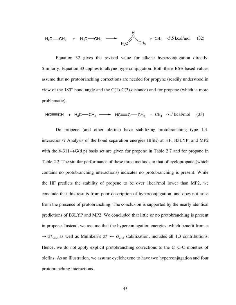
45

Equation 32 gives the revised value for alkene hyperconjugation directly.

Similarly, Equation 33 applies to alkyne hyperconjugation. Both these BSE-based values

assume that no protobranching corrections are needed for propyne (readily understood in

view of the 180° bond angle and the C(1)-C(3) distance) and for propene (which is more

problematic).

Do propene (and other olefins) have stabilizing protobranching type 1,3-

interactions? Analysis of the bond separation energies (BSE) at HF, B3LYP, and MP2

with the 6-311++G(d,p) basis set are given for propene in Table 2.7 and for propane in

Table 2.2. The similar performance of these three methods to that of cyclopropane (which

contains no protobranching interactions) indicates no protobranching is present. While

the HF predicts the stability of propene to be over 1kcal/mol lower than MP2, we

conclude that this results from poor description of hyperconjugation, and does not arise

from the presence of protobranching. The conclusion is supported by the nearly identical

predictions of B3LYP and MP2. We concluded that little or no protobranching is present

in propene. Instead, we assume that the hyperconjugation energies, which benefit from !

" !*CH3 as well as Mulliken’s !* # !CH3 stabilization, includes all 1,3 contributions.

Hence, we do not apply explicit protobranching corrections to the C=C-C moieties of

olefins. As an illustration, we assume cyclohexene to have two hyperconjugation and four

protobranching interactions.

46

Table 2.7. BSE analysis of propene. The E0 (electronic) and the ZPE/Thermal (scaled

zero-point vibrational and thermal corrections to 298K) are in kcal/mol. All computations

used the 6-311++G(d,p) basis set.

propene + methane " ethene + ethane

Level E0 ZPE/Thermal E0 + ZPE/Thermal

HF 3.74 0.54 4.28

B3LYP 4.70 0.50 5.20

MP2 4.99 0.40 5.39

Experiment 5.71

We have also made use of an entirely different approach to quantify the effect of

electron delocalization on unsaturated systems, the block-localized wave function (BLW)

method of Mo et al.[62,63] BLW is closely associated with valence bond (VB) theory and

can be employed at the practicable HF and DFT levels, because of error cancellation. The

wave function of the major contributor to a resonance hybrid, e.g., a localized, non-

conjugating cyclohexatriene, can be optimized self-consistently. In effect, BLW “turns

off” the ! conjugation in butadiene, the hyperconjugation in propene, and the aromaticity

in benzene, but the sigma framework remains essentially intact. As an illustration,

Equation 33 is not balanced with regard to the number of C(sp2)-X and C(sp3)-X bonds

(X=H or C), but the BLW method applied to propene does not have this fault. BLW thus

affords a considerable conceptual advantage over conventional delocalization energy

assessments using thermochemical data and isodesmic or homodesmotic reactions. Such

reactions attempt to approximate a virtual Lewis structure (the most stable resonance

structure), in which the effects of electron delocalization are absent, as a composite of

non-delocalized model reference compounds. In contrast, the difference between the

47

BLW and HF (or KS) wave functions of the same compound gives the resonance energy

(following the Pauling-Wheland definition) directly. The BLW method already has been

applied to many molecules,[63-68] including the evaluation of the hyperconjugation of

propene and the aromaticity of benzene.

The validity of our revised hyperconjugation energy of propene is substantiated

by the BLW method. For propene, the delocalized (HF or KS) and localized (BLW) wave

functions can be expressed as

( ) ( )2221del aaA !!!!!=" #ˆ

and

( ) ( )22

3

locCHCC

A !!" =#=$ ˆ

where !C=C and !CH3 are group orbitals expanded in CH2=CH and CH3 groups, and are

nonorthogonal. In contrast, 1a" and 2a" are delocalized for the whole system and

orthogonal. The energy difference between these two functionals, which are

independently optimized self-consistently, represents the vicinal interaction between the

! double bond and the adjacent methyl group, or more simply the hyperconjugation of

the methyl group. Using the 6-311+G(d,p) basis set the adiabatic hyperconjugation

energy is estimated to be -5.5 or -6.3 kcal/mol at the HF or DFT (B3LYP) level, in

agreement with the -5.5 kcal/mol obtained in Equation 32.

Recently Rogers et al. developed an increment scheme for estimating the heats of

formation of polyynes.[69] While the increment scheme reproduces both theoretically and

experimentally derived heats of formation accurately, we criticize the evaluation methods

to achieve these increments. Our derivation of the energies of protobranching,

48

hyperconjugation, conjugation, as well as what we have termed “cross-hyperconjugation”

for Rogers’ compounds, gives a different perspective.

The BSE of n-pentane (8.59 kcal/mol), 1-pentyne (13.24 kcal/mol), and 1,3-

pentadiyne (23.67 kcal/mol) were computed using G3(MP2) data.[70] The BSE for n-

pentane provides 2.86 kcal/mol per protobranching stabilization. Hyperconjugation (7.58

kcal/mol) is given by the BSE of 1-pentyne after correction for the two protobranches

present. Diyne conjugation stabilization is 16.09 kcal/mol, based on the BSE of 1,3-

pentadiyne after subtracting the value of a methyl hyperconjugation.

Cross hyperconjugation, involving the attenuated interaction of a methylene group

situated between two triple bonds, is present in 1,4-hexadiyne. Its BSE, 21.51 kcal/mol,

minus the methyl hyperconjugation, defines this stabilization, 13.93 kcal/mol. This is

only about 1.2 kcal/mol less than two individual alkyne hyperconjugations (2 x 7.58

kcal/mol = 15.16 kcal/mol), in sharp contrast to the 3.9 kcal/mol destabilization assigned

by Rogers et al. An extensive list of BSE values of unsaturated compounds is given in

Table 2.8.

While Rogers et al.’s self-consistent increment scheme accurately reproduces

experimental heats of formation, we take issue with their derivation of the stabilization

energy values for conjugation and cross hyperconjugation. Since hyperconjugation was

not considered, the 0.9 kcal/mol attributed to “conjugation” and the 3.9 kcal/mol

destabilization due to “attenuation” do not represent the uncontaminated values.

Fortuitous cancellation can result in data-fitting schemes, which predict accurate values

of heats of formation, but do not have interpretive significance.[20] Diynes are stabilized

much more than 0.9 kcal/mol by conjugation; the BSE value is 15.1 kcal/mol.

49

Based on the BLW method, the Pauling-Wheland resonance (conjugation) energy

in 1,3-butadiyne is even larger, 20.1 kcal/mol at the HF/6-311+G(d,p) level (26.2

kcal/mol at B3LYP/6-311+G(d,p) level). The BLW resonance energy of anti-1,3-

butadiene (9.9 kcal/mol at the HF/6-311+G(d,p) level and 12.2 kcal/mol at the B3LYP/6-

311+G(d,p) level) is half as large. The difference between the BSE and BLW diyne

estimates (see summary Table 2.9 in the Conclusions) may be due to differences in the

carbon hybridization in the isodesmic bond separation reactions.

50

Table 2.8. Evaluation of bond separation energies for unsaturated hydrocarbons (in kcal/mol). NIST thermochemical data at 298K

were employed.

Molecule

PB Alkene

HC

Alkyne

HC

Alkene

CHC

Alkyne

CHC

Alkene

Conj

Alkyne

Conj

Est Energy Bond

Separation

Energy

propane 1 -- -- -- -- -- -- 2.83 2.83

propene -- 1 -- -- -- -- -- 5.71 5.71

propyne -- -- 1 -- -- -- -- 7.81 7.81

1-butene 1 1 -- -- -- -- -- 8.54 8.58

trans-2-butene -- 2 -- -- -- -- -- 11.42 11.01

2-methyl-1-propene 1 2 -- -- -- -- -- 14.25 12.54

anti-1,3-butadiene -- -- -- -- -- 1 -- 14.84 14.84

syn-1,3-butadiene -- -- -- -- -- 1 -- 12.94 12.94

1-butyne 1 -- 1 -- -- -- -- 10.64 10.41

2-butyne -- -- 2 -- -- -- -- 15.62 15.21

1,3-butadiyne -- -- -- -- -- -- 1 15.12 15.12

trans-1,3-pentadiene -- 1 -- -- -- 1 -- 20.55 20.50

1,4-pentadiene 1 -- -- 1 -- -- -- 13.26 13.26

1,3-pentadiyne -- -- 1 -- -- -- 1 22.93 23.67

1-pentene 2 1 -- -- -- -- -- 11.37 11.19

trans-2-pentene 1 2 -- -- -- -- -- 14.25 14.00

1-pentyne 2 -- 1 -- -- -- 13.47 13.24

2-pentyne 1 -- 2 -- -- -- -- 18.45 16.94

51

1-hexene 3 1 -- -- -- -- -- 14.20 14.35

3-hexene 2 2 -- -- -- -- -- 17.08 16.95

cyclohexene 4 2 -- -- -- -- -- 22.74 20.72

1,3-cyclohexadiene 2 2 -- -- -- 1 -- 30.02 27.28

1,4-hexadiyne -- -- 1 -- 1 -- -- 21.72 21.72

1,5-hexadiyne 2 -- 2 -- -- -- -- 21.28 20.52

1,3,5-hexatriyne -- -- -- -- -- -- 2 30.24 30.65

3-heptyne 3 -- 2 -- -- -- -- 24.11 23.04

1,3-heptadiyne 2 -- 1 -- -- -- 1 28.59 29.37

1,3,6-heptatriyne -- -- -- -- 1 -- 1 29.03 29.50

52

2.3.6. PROTOBRANCHING AND AROMATIC RESONANCE (RE) AND

STABILIZATION ENERGIES (ASE)

Kistiakowsky’s seminal evaluation of the resonance energy of benzene (Equation 6,

Scheme 2.1)[71] has previously been criticized.[67] His 36 kcal/mol value,[71] based on the

heats of hydrogenation of benzene and cyclohexene, is badly flawed, since the three

reference cyclohexenes on the right side are stabilized considerably by hyperconjugation

(a concept unknown at that time), for which there is no compensation on the left side.

Consequently, the RE of benzene must be much larger than 36 kcal/mol.

Many model reactions (isodesmic, homodesmotic, etc.) have been used to

estimate the resonance energy (RE) as well as the aromatic stabilization energy (ASE) of

benzene.[72] According to Pauling and Wheland resonance energy is defined as the

difference between the actual energy of a molecule and the virtual energy of the most

stable resonance contributor.[73-77] Since the real reference molecules chosen to

approximate the virtual energy of a non-resonating cyclohexatriene are never free from

other stabilizing or destabilizing interactions, these perturbing features

(“contaminations”) should be balanced in the defining equations as completely as

possible. Unfortunately, Equations 35-39 Scheme 2.2 fail to balance the stabilization

from conjugation, hyperconjugation, and protobranching interactions.

53

Scheme 2.2. Equations that have been employed to evaluate the resonance energy of

benzene. The upper values are the original RE estimates. The lower values are the RE’s

after correction for the perturbing effects of protobranching, hyperconjugation, and

conjugation.

A second set of ASE evaluations, devised to compare benzene with conjugation

but non-aromatic reference molecules, have been widely discussed in the literature.[78]

Consequently, the various equations used to estimated the stabilization of the benzene RE

and ASE give very different values. The wide divergence of benzene stabilization

energies often has been mentioned disparagingly in critical appraisals of the aromaticity

54

concept. Remarkably, when hyperconjugation, protobranching, and conjugation

adjustment are applied, the various aromaticity evaluations (Equations 34-39) yield

surprisingly consistent resonance energies!

The BSE (Equation 34 of Scheme 2.2) gives a RE equal to 64.39 kcal/mol and

requires no modification for hyperconjugation and protobranching, as these are not

involved. Equation 35, evaluated directly using 298K experimental data, gives a much

lower value, 48.25 kcal/mol. However, the stabilizing 1,3-alkyl-alkyl protobranching

interactions of the cyclohexane reference molecule should be considered. Adding the

stabilization from protobranching corrects the Equation 35 RE to 65.50 kcal/mol. This is

nearly identical with the RE from Equation 34!

Kistiakowsky originally applied isodesmic Equation 36 to give the RE of

benzene.[71] However, the flaws in this equation are now apparent. While protobranching

is balanced (four for each of the three cyclohexenes on the left vs. six each for the two

cyclohexanes on the right side), the total of six stabilizing hyperconjugative interactions

on the left side (worth 5.7 kcal/mol each, see above) have no counterpart on the right.

When this hyperconjugation stabilization is taken into account, the RE given by Equation

36 increases from 36.0 to 70.2 kcal/mol.

Equation 37 was devised to estimate the ASE of benzene, but also can serve (after

correction) to assess its RE. The total of six hyperconjugative and twelve protobranches

are balanced, but three uncompensated syn-type conjugation interactions (worth 12.94

kcal/mol each) are present on the left side. Their consideration results in a benzene RE of

67.3 kcal/mol. The three uncompensated conjugations in Equation 38 and 39 stabilize the

left sides by 44.52 kcal/mol; when this is taken into account, the RE of Equation 38 is

55

increased from 20.5 to 65.1 kcal/mol and of Equation 39 from 22.5 kcal/mol to 67.0

kcal/mol.

Clearly contributions from conjugation, hyperconjugation, and protobranching

should be considered when evaluating resonance energies. After correcting for these

effects, the inconsistencies in RE’s given by Equation 34-39 largely vanish (Figure 2.6).

Figure 2.6. Original values and stabilization revised values for aromatic stabilization

energies calculated by various equations (Scheme 2.2).

Dewar’s original definition of the aromatic stabilization energy (ASE), Equation

40 in Scheme 2.3, is intended to estimate the extra resonance energy due to the cyclic

electron delocalization.[79] The ASE of Equation 40 is 20.53 kcal/mol. However, benzene

only has syn conformations, which, for 1,3-butadiene, are 3.0 kcal/mol higher in energy

56

than the anti conformations. Equation 41, employing the 1,3-cyclohexadiene as the

reference, removes the syn/anti discrepancy (as well as balances all protobranching and

hyperconjugation interactions) and results our recommended ASE value, of 28.48

kcal/mol. This value agrees well with the mathematical derivation of Dewar resonance

energy, 32.7 kcal/mol, obtained by Fishtik and Datta.[80]

Scheme 2.3. Equations used to evaluate aromatic stabilization energy of benzene.

57

2.4 CONCLUSIONS

Protobranching is a simple concept with remarkably broad, paradigm shifting

implications for energy evaluations in organic chemistry. Protobranching extends the

well-established concept of branching to n-alkanes and to cycloalkanes. The

consequences for energetic analysis are fundamental: n-alkanes larger than ethane and

cyclohexane can no longer be considered “strain-free” reference molecules. All

interactions, other than the one of interest, should be balanced in reference molecules, but

this is difficult to realize in larger systems. Unblemished energetic analysis requires the

elimination of all contaminants, either stabilizing or destabilizing, with reference

molecules. This can be achieved best by using simple molecules (methane, ethane,

ethene, etc.), which provide references that lack perturbing effects (e.g., conjugation,

hyperconjugation, and strain, as well as protobranching). The recognition of

protobranching adds another effect that should be considered. If this is not done,

incomplete and potentially misleading energetic analyses will result.

The protobranching concept accounts for the very large errors, e.g., in estimates

of branching energies as well as the heats of formation of the larger n-alkanes by HF and

B3LYP as well as other DFT functionals. Application of the protobranching concept

reduces the conventional strain energy of cyclopropane from 27.7 to 19.2 kcal/mol, and

also reduces the conventional ring strain estimates of cyclobutane, tetrahedrane, and

cubane to much smaller values.

Protobranching also helps reconcile the inconsistent values, ranging from 19.3 to

66.9 kcal/mol, for the benzene stabilization energy given by many literature schemes.[78]

Agreement is achieved when conjugation, hyperconjugation, and protobranching

58

corrections are applied. Kistiakowsky’s classical resonance energy,[71] 36 kcal/mol, is

underestimated due to the neglect of hyperconjugation; we recommend the BSE value of

64.4 kcal/mol instead. The ASE of benzene is revised from 20.5 to 28.8 kcal/mol.

When protobranching is taken into account, the conventional hyperconjugative

stabilization of an alkene by an alkyl group more than doubles, from 2.5 to 5.5 kcal/mol.

The BLW value is 5.5 kcal/mol (6.3 kcal/mol B3LYP). The alkyl group alkyne

hyperconjugation increases from 5.0 to 7.7 kcal/mol, based on BSE; the BLW value is

even larger (10.5 kcal/mol HF, 12.5 kcal/mol B3LYP). Consideration of protobranching

increases estimation of the conjugation energy of dienes from 3.7 to 14.8 kcal/mol (BLW

9.9 kcal/mol HF, 12.2 kcal/mol B3LYP) and diynes from 0.2 to 15.1 kcal/mol (BLW 20.1

kcal/mol HF, 26.2 kcal/mol B3LYP). Table 2.9 summarizes our major thermochemical

and BLW evaluations with the conventional values.

59

Table 2.9. Summary of conventional, revised, and BLW (at HF and B3LYP) energy

evaluations of strain, hyperconjugation, conjugation, and benzene aromaticity (kcal/mol).

Property Conventional

Evaluation

Revised

Evaluation

(Based on BSE)

BLW Evaluation

(B3LYP)

Ring/Cage Strain

cyclopropane 27.7 19.2 --

cyclobutane 26.8 21.0a --

tetrahedrane 136.3 105.4 --

cubane 164.8 102.9a --

Hyperconjugation

propene 2.5 5.7 5.4 (6.3)

propyne 5.0 7.8 10.5 (12.5)

Conjugation

butadiene 3.7 14.8 9.9 (12.2)

butadiyne 0.2 15.1 20.1 (26.2)

Aromaticity of

Benzene

ASE 20.5 28.8 --

RE 36.0 64.4 57.5 (63.2)

a Corrected for protobranching; see text.

2.6 ACKNOWLEDGMENTS

We thank C. Corminboeuf and N. L. Allinger for helpful discussions. Computations were

partially performed at the University of Georgia Research Computing Center. NSF Grant

CHE-0209857 and the Petroleum Research Fund supported our work.

60

2.7 REFERENCES

[1] M. Faraday, Phil. T. 1825, 115, 440.

[2] A. Kekulé, Lehrbuch der Organischen Chemie, Enke, Erlangen, 1866.

[3] A. Baeyer, Ber. Dtsch. Chem. Ges. 1885, 18, 2269.

[4] J. Thiele, Annalen 1899, 87, 306.

[5] J. Rossini, Research Natl. Bur. Standards 1934, 13, 21.

[6] C. D. Nenitzescu, I. Chicos, Ber. Dtsch. Chem. Ges. 1935, 68B, 1584.

[7] R. S. Mulliken, J. Chem. Phys. 1939, 7, 339.

[8] R. S. Mulliken, C. A. Rieke, W. G. Brown, J. Am. Chem. Soc. 1941, 63, 41.

[9] H. Y. Afeefy, J. F. Liebman, S. E. Stein, Neutral Thermochemical Data. In NIST

Chemistry Webbook, NIST Standard Reference Database Number 69, P. J. Linstrom, W.

G. Mallard, Eds., National Institute of Standards and Technology: Gaithersburg, MD

(http://webbook.nist.gov).

[10] P. v. R. Schleyer, 229th National Meeting of the American Chemical Society (San

Diego, CA) 2005.

[11] M. D. Wodrich, P. v. R. Schleyer, 37th Middle Atlantic Regional Meeting of the

American Chemical Society (New Brunswick, NJ) 2005.

[12] M. D. Wodrich, C. Corminboeuf, P. v. R. Schleyer, Org. Lett. 2006, 8, 3631.

61

[13] T. L. Allen, J. Chem. Phys. 1959, 29, 951.

[14] T. L. Allen, J. Chem. Phys. 1959, 31, 1039.

[15] M. Cignitti, T. L. Allen, J. Am. Chem. Soc. 1965, 43, 4472.

[16] V. N. Ipatieff, A. V. Grosse, Ind. Eng. Chem. 1936, 28, 461.

[17] G. A. Olah, A. Molnár, Hydrocarbon Chemistry, John Wiley & Sons, New York,

1995.

[18] K. Fajans, Ber. Dtsch. Chem. Ges. 1920, 53B, 643.

[19] H. Eyring, J. Am. Chem. Soc. 1932, 54, 3191.

[20] S. Gronert, J. Org. Chem. 2006, 71, 1209.


[22] M. D. Wodrich, P. v. R. Schleyer, Org. Lett. 2006, 8, 2135.

[23] S. Grimme, Angew. Chem. Int. Ed. 2006, 45, 4460.

[24] K. S. Pitzer, E. Catalano, J. Am. Chem. Soc. 1956, 78, 4844.

[25] F. London, Trans. Faraday Soc. 1937, 33, 8.

[26] W. J. Hehre, R. Ditchfield, L. Radom, J. A. Pople, J. Am. Chem. Soc. 1970, 92,

4796.

[27] L. Radom, W. J. Hehre, J. A. Pople, J. Am. Chem. Soc. 1971, 93, 289.

62

[28] W. J. Hehre, L. Radom, P. v. R. Schleyer, J. A. Pople, Ab Initio Molecular Orbital

Theory, John Wiley & Sons, New York, 1986.

[29] P. George, M. Trachtman, C. W. Bock, A. M. Brett, Tetrahedron 1976, 32, 317.

[30] P. George, M. Trachtman, A. M. Brett, C. W. Bock, J. C. S. Perkin II 1977, 8, 1036.

[31] Experimental data for higher n-alkanes at 298K actually refer to Boltzmann

distributions of various conformations`; this progressive complication contributes to the

uncertainty of individual values, but has not been considered here.

[32] L. A. Gribov, I. A. Novakov, A. I. Pavlyuchko, O. Kulago, B. S. Orlinson, J. Struct.

Chem. 2003, 44, 961.

[33] X. Wu, M. C. Vargas, S. Nayak, V. Lotrich, G. Scoles, J. Chem. Phys. 2001, 115,

8748.

[34] U. Zimmerli, M. Parrinello, P. Koumoutsakos, J. Chem. Phys. 2004, 120, 2693.

[35] O. A. von Lilienfeld, I. Tavernelli, U. Rothlisberger, D. Sebastiani, Phys. Rev. Lett.

2004, 93, 153004.

[36] T. Sato, T. Tsuneda, K. Hirao, Mol. Phys. 2005, 103, 1151.

[37] Y. Zhao, D. G. Truhlar, J. Chem. Theory Comput. 2005, 1, 415.

[38] C. E. Check, T. M. Gilbert, J. Org. Chem. 2005, 70, 9828.

[39] P. R. Schreiner, A. A. Fokin, R. A. Pascal, Jr. , A. de Meijere, Org. Lett. 2006, 8,

3635.

63

[40] Gaussian 98, Revision A.11, M. J. Frisch, G. W. Trucks, H. B. Schlegel, G. E.

Scuseria, M. A. Robb, J. R. Cheeseman, V. G. Zakrewksi, J. A. J. Montgomery, R. E.

Stratman, J. C. Burant, S. Dapprich, J. M. Millam, A. D. Daniels, K. N. Kudin, M. C.

Strain, O. Farkas, J. Tomasi, V. Barone, M. Cossi, R. Cammi, B. Mennucci, C. Pomelli,

C. Adamo, S. Clifford, J. Ochterski, G. A. Petersson, P. Y. Ayala, Q. Cui, K. Morokuma,

D. K. Malick, A. D. Rabuck, K. Raghavachari, J. B. Foresman, J. Cioslowski, J. V. Ortiz,

B. B. Stefanov, G. Liu, A. Liashenko, P. Piskorz, I. Komaromi, R. Gomperts, R. L.

Martin, D. Fox, T. Keith, M. A. Al-Laham, C. Y. Peng, A. Nanayakkara, C. Gonzalez,

M. Challacombe, P. M. W. Gill, B. G. Johnson, W. Chen, M. W. Wong, J. L. Andes, M.

Head-Gordon, E. S. Replogle, J. A. Pople, Gaussian, Inc.: Pittsburgh, 1998.

[41] Gaussian 03, Revision C.02, M. J. Frisch, G. W. Trucks, H. B. Schlegel, G. E.

Scuseria, M. A. Robb, J. R. Cheeseman, J. A. Montgomery, Jr., T. Vreven, K. N. Kudin,

J. C. Burant, J. M. Millam, S. S. Iyengar, J. Tomasi, V. Barone, B. Mennucci, M. Cossi,

G. Scalmani, N. Rega, G. A. Petersson, H. Nakatsuji, M. Hada, M. Ehara, K. Toyota, R.

Fukuda, J. Hasegawa, M. Ishida, T. Nakajima, Y. Honda, O. Kitao, H. Nakai, M. Klene,

X. Li, J. E. Knox, H. P. Hratchian, J. B. Cross, V. Bakken, C. Adamo, J. Jaramillo, R.

Gomperts, R. E. Stratmann, O. Yazyev, A. J. Austin, R. Cammi, C. Pomelli, J. W.

Ochterski, P. Y. Ayala, K. Morokuma, G. A. Voth, P. Salvador, J. J. Dannenberg, V. G.

Zakrzewski, S. Dapprich, A. D. Daniels, M. C. Strain, O. Farkas, D. K. Malick, A. D.

Rabuck, K. Raghavachari, J. B. Foresman, J. V. Ortiz, Q. Cui, A. G. Baboul, S. Clifford,

J. Cioslowski, B. B. Stefanov, G. Liu, A. Liashenko, P. Piskorz, I. Komaromi, R. L.

Martin, D. J. Fox, T. Keith, M. A. Al-Laham, C. Y. Peng, A. Nanayakkara, M.

64

Challacombe, P. M. W. Gill, B. Johnson, W. Chen, M. W. Wong, C. Gonzalez, and J. A.

Pople, Gaussian, Inc., Wallingford CT, 2004.


[43] CCSD(T) energies were computed using single point calculations at the MP2/6-

311++G(d,p) geometry as well as MP2 ZPE and thermal corrections.

[44] N. Cohen, S. W. Benson, Chem. Rev. 1993, 93, 2419.

[45] K. E. Laidig, J. Phys. Chem. 1991, 95, 7709.

[46] K. S. Pitzer, J. Chem. Phys. 1937, 5, 469.

[47] K. S. Pitzer, Science 1945, 101, 672.

[48] V. Pophristic, L. Goodman, Nature 2001, 411, 565-568.

[49] K. Exner, P. v. R. Schleyer, J. Phys. Chem. A 2001, 105, 3407.

[50] D. Cremer, J. Gauss, J. Am. Chem. Soc. 1986, 108, 7467.

[51] J. D. Dunitz, V. Schomaker, J. Chem. Phys. 1952, 20, 1703.

[52] N. L. Bauld, J. Cessac, J. Am. Chem. Soc. 1977, 99, 942.

[53] N. L. Bauld, J. Cessac, R. L. Holloway, J. Am. Chem. Soc. 1977, 99, 8140.

[54] Tetrahedrane heat of formation calculated from G2 theory. See M. N. Glukhovtsev,

S. Laiter, A. Pross, J. Phys. Chem. 1995, 99, 6828.

65

[55] M. N. Glukhovtsev, S. Laiter, A. Pross, J. Phys. Chem. 1995, 99, 6828.

[56] D. Moran, M. Manoharan, T. Heine, P. v. R. Schleyer, Org. Lett. 2003, 5, 23.

[57] M. M. Balci, M. L.; Schleyer, P. v. R., J. Phys. Chem. A 2000, 104, 1246.

[58] R. D. Cox, G. Pilcher, Thermochemistry of Organic and Organometallic

Compounds, Academic Press, New York, 1970.

[59] P. v. R. Schleyer, J. E. Williams, K. R. Blanchard, J. Am. Chem. Soc. 1970, 92,

2377.

[60] J. Hine, Structural Effects of Equilibria in Organic Chemistry, John Wiley & Sons,

New York, 1975.

[61] P. D. Jarowski, M. D. Wodrich, C. S. Wannere, P. v. R. Schleyer, K. N. Houk, J.

Am. Chem. Soc. 2004, 126, 15036.

[62] Y. Mo, S. D. Peyerimhoff, J. Chem. Phys. 1998, 109, 1687.

[63] Y. Mo, P. v. R. Schleyer, W. Wu, M. H. Lin, Q. Zhang, J. L. Gao, J. Phys. Chem. A

2003, 107, 10011.

[64] Y. Mo, J. L. Gao, S. D. Peyerimhoff, J. Chem. Phys. 2000, 112, 5530.

[65] Y. Mo, L. C. Song, W. Wu, Q. N. Zhang, J. Am. Chem. Soc. 2004, 126, 3974.

[66] Y. Mo, J. Org. Chem. 2004, 69, 5563.

[67] Y. Mo, P. v. R. Schleyer, Chem. Eur. J. 2006, 12, 2009.

66

[68] Y. Mo, Org. Lett. 2006, 8, 535.

[69] D. W. Rogers, N. Matsunaga, F. J. McLafferty, A. A. Zavitsas, J. F. Liebman, J.

Org. Chem. 2004, 69, 7143.

[70] L. A. Curtiss, P. C. Redfern, K. Raghavachari, V. Rassolov, J. A. Pople, J. Chem.

Phys. 1999, 110, 4703.

[71] G. B. Kistiakowsky, J. R. Ruhoff, H. A. Smith, W. E. Waughan, J. Am. Chem. Soc.

1936, 58, 146.

[72] L. G. Wade, Organic Chemistry, Prentice Hall, Upper Saddle River, 1999.

[73] L. C. Pauling, G. W. Wheland, J. Chem. Phys. 1933, 1, 362.

[74] L. C. Pauling, The Nature of the Chemical Bond, Cornell University Press, Ithaca,

1960.

[75] G. W. Wheland, J. Am. Chem. Soc. 1941, 63, 2025.

[76] G. W. Wheland, The Theory of Resonance, John Wiley & Sons, New York, 1944.

[77] G. W. Wheland, Resonance in Organic Chemistry, Wiley, New York, 1955.

[78] M. K. Cyranski, Chem. Rev. 2005, 105, 3773.

[79] M. J. S. Dewar, H. N. Schmeising, Tetrahedron 1959, 5, 166.

[80] I. Fishtik, R. Datta, J. Phys. Chem. A 2003, 107, 10471.

CHAPTER 3

NEW ADDITIVITY SCHEMES FOR HYDROCARBON ENERGIES†

† Matthew D. Wodrich and Paul von Ragué Schleyer. Organic Letters 2006, 8, 2135.

Copyright 2006 American Chemical Society.

68

3.1. ABSTRACT

A new isodesmic additivity scheme based on the energetic relationships among the

simplest hydrocarbon molecules reproduces the experimental heats of formation for a

broad range of unstrained hydrocarbons with remarkable accuracy. The stabilizations of

radicals, double, and triple CC bonds by alkyl substituents (hyperconjugation), as well as

the stabilization by 1,3-alkyl group interactions at the same carbon (branching) support

conventional interpretations. Statistical data fitting can also be achieved by using only

four adjustable parameters.

3.2. INTRODUCTION

Decades of meticulous experimental measurements provided accurate thermochemical

data for a large number of hydrocarbons.[1] Regularities in these data have been expressed

by many quantitative relationships, most notably the extensive group increment scheme

developed and refined by Benson.[2] Assuming additivity, increment values for e.g., C-

(C)(H)3, C-(C)2(H)2 and many other hydrocarbon groups reproduce the known heats of

formation (!Hf) remarkably well (see the selection in Table 3.1). Deviations from

additivity can be used, for example, to evaluate “strain” but the main purpose of these

increments is predictive, rather than interpretive. The many increment types required by

Benson’s method are evaluated by averaging all the available experimental data. In the

present context, Benson’s method requires nine group enthalpy increments for the

selection of alkanes, alkenes, and alkynes listed in Table 3.1, a separate value for

methane, and a special treatment for the alkyl radicals.[2]

69

Table 3.1. Heats of formation of Gronert’s strain–free hydrocarbons as well as alkynes,

in kcal/mol. Molecules shown in bold font were used to derive the isodesmic parameters

and attenuation coefficients employed in Scheme 3.2 and Table 3.2.

Molecule Experimental

Refs. 1, 7

Benson[2]

Benson

Deviation

Gronerta,b

Gronert

Deviation

Isodesmic Isodesmic

Deviation

methane -17.89 -- -- -17.3 0.6 -17.89 0.0

ethane -20.04 ± 0.07 -20.00 0.0 -20.4 0.3 -20.04 0.0

propane -25.02 ± 0.12 -25.00 0.0 -25.3 0.3 -25.02 0.0

n-butane -30.03 ± 0.16 -30.00 0.0 -30.2 0.2 -30.00 0.0

isobutane -32.07 ± 0.15 -32.40 0.3 -31.9 0.2 -32.08 0.0

n-pentane -35.08 ± 0.14 -35.00 0.1 -35.1 0.0 -34.98 0.1

isopentanec -36.73 ± 0.14 -36.60 0.1 -36.8 0.1 -37.06 0.3

Neopentane -40.14 ± 0.15 -40.10 0.0 -40.3 0.2 -39.98 0.2

n-hexane -39.96 ± 0.19 -40.00 0.0 -40.0 0.0 -39.96 0.0

n-heptane -44.89 ± 0.19 -45.00 0.1 (-45.1) 0.2 -44.94 0.1

Cyclohexane -29.43 ± 0.19 -29.30d 0.1 -29.3 0.1 -29.88 0.5

trans-decalin -43.54 ± 0.55 -44.80 1.3 (-41.8) 2.8 -43.89 0.4

methyl radical 35.05 ± 0.07i -- -- 34.9 0.1 35.05 0.0

ethyl radical 29.0 ± 0.4i 28.4 0.0 29.1 0.1 29.00 0.0

n-propyl radical 23.9 ± 0.5 23.4 0.5 24.2 0.3 24.02 0.1

isopropyl radical 21.5 ± 0.4i 21.0 1.0 21.6 0.1 21.29 0.2

sec-butyl radical 16.1 ± 0.5i 16.0 0.0 16.7 0.6 16.31 0.2

tert-butyl radical 12.3 ± 0.4i 11.0 1.3 12.2 0.1 12.40 0.1

cyclohexyl radical No data 16.0 -- (17.5) -- 16.43 --

Ethene 12.54 12.54 0.0 12.5 0.0 12.54 0.0

Propene 4.88 4.82 0.1 4.9 0.0 4.88 0.0

1-butene -0.15 ± 0.19 -0.18 0.0 0.1 0.3 -0.10 0.1

E-2-butene -2.58 ± 0.24 -2.90 0.3 -2.6 0.0 -2.78 0.2

2-methylpropene -4.29 ± 0.26 -3.54 0.8 -4.3 0.0 -4.29 0.0

2-methyl-2-butene -9.92 ± 0.21 -10.12 0.2 -10.1 0.2 -10.25e 0.3

tetramethylethylene -16.80 ± 0.36 -17.42 0.6 (-21.6) 4.8 -17.06e 0.3

Acetylene 54.19 ± 0.19 54.20 0.0 -- -- 54.19 0.0

Propyne 44.32 ± 0.21 44.40 0.1 -- -- 44.32 0.0

1-butyne 39.48 ± 0.21 39.66 0.2 -- -- 39.34 0.2

2-butyne 34.68 ± 0.24 34.60 0.1 -- -- 34.45 0.2

1-pentyne 34.50 ± 0.50 34.67 0.2 -- -- 34.36 0.1

2-pentyne 30.80 ± 0.50 29.86 0.9 -- -- 29.47 1.3

3-methyl-1-butyne 32.60 ± 0.50 32.86 0.3 -- -- 32.28 0.3

3,3-dimethyl-1-butyne 25.36 25.72 0.4 -- -- 24.38 1.0

a) Data given by Gronert (reference 3) or (in parentheses) derived here from his scheme. b) Acetylenes

were not considered by Gronert. c) Isopentane is strained, but the gauche interaction is ignored. d)

Benson’s 0.7 kcal/mol strain correction was included. e) Including 2.03 kcal/mol cis strain corrections. See

text.

70

Recently, Gronert[3] devised a new additivity scheme based on fewer parameters, which

is remarkable in reproducing accurately the !Hf‘s of diverse unstrained hydrocarbons,

alkanes, alkyl radicals, and alkenes (Table 3.1), by means of a unified treatment (Scheme

3.1a). But Gronert went far beyond this empirical success to claim validity for the

assumptions he employed (notably geminal repulsions) in devising his scheme and to

question well-established concepts like hyperconjugation. We now analyze Gronert’s

treatment in detail and show that the simpler Scheme 3.1b, with a single, attractive

geminal term, is able to reproduce the same set of experimental data satisfactorily. Our

second treatment, Scheme 3.2, based on conventional reasoning, performs equally well.

Gronert’s Scheme 3.1a is easy to use in practice. It depends on the number of each kind

of bond (two-atom terms) and 1,3–geminal combination (three-atom terms). The H atom

!Hf = 52.1 kcal/mol, used in the one-atom f(C,H) term, is the only directly employed

experimental value. In contrast, Gronert did not employ the experimental DHf = 170.6

kcal/mol for the C atom, but increased its value to 231.3 kcal/mol by adding 60.7

kcal/mol (the bond dissociation energy of the excited C–H quartet state). Gronert then

derived his C–C, C=C, and C–H bond energies arbitrarily by statistical fitting; the

resulting values are very far from conventional estimates (see discussion below). The

values of these bond energies are artificially assumed to be the same for all hydrocarbons

(independent of carbon hybridization, etc.) and serve to decrease the total energy.

Three additional statistically derived CCC, CCH, and HCH three-atom geminal

interaction terms increase the energy. These terms depend only on the number of each

type of geminal unit, and are independent of the actual structure.

71

Scheme 3.1. (a) Gronert’s method for evaluating alkane, cycloalkane, alkene, and alkyl

radical heats of formation. (b) Four-parameter simplification employing experimental H

and C data. (See Tables 3.5 and 3.19.)

!Hf = nC-CEC-C + nC=CEC=C + nC-HEC-H + nC-C-CEC-C-C +

nC-C-HEC-C-H + nH-C-HEH-C-H – f(C,H)

a) Gronert’s evaluation (including CH and CH2): f(C,H) = (170.6 + Ec)nC + 52.1 nH) EC-C = –146.0, EC=C = -

–66.2, EC-H = –124.2, EC-C-C = 10.2, EC-C-H = 9.3, EH-C-H = 6.6, and EC = 60.7 kcal/mol.

b) Four-parameter simplification (excluding CH and CH2): f(C,H) = (170.6 nC + 52.1 nH), EC-C = –85.59,

EC-H = –96.07, EC=C = –64.34, EH-C-H = -1.97

72

To summarize, Scheme 3.1a achieves its diversity of application and accuracy by

employing the fixed values of seven arbitrarily derived terms. The value for f(C) is set ad

hoc and the values of the other terms are determined empirically as best fit averages of

the experimental hydrocarbon heats of formation shown in Table 3.1. Only f(H) is based

directly on the experimental !Hf value.

Gronert conceded that his derived C–C and C–H bond energy values are far larger than

those commonly accepted in the literature. For instance, the conventional average C–H

bond energy (BE) of methane (99.2 kcal/mol) is ! the experimental atomization energy

(396.9 kcal/mol). Gronert’s C–H value is 124.2 kcal/mol. Assuming that ethane has the

same C-H BE as methane (an assumption Gronert adopts), the experimentally-based C-C

BE of ethane is 78.5 kcal/mol.[4] The experimental CC bond dissociation energy (BDE) of

ethane into two methyl radicals is 91.4 kcal/mol. Gronert’s 146.0 kcal/mol C-C value is

much larger that both the ethane BE and BDE, and has no independent support. As the

one-atom and two-atom terms in Scheme 3.1a result in !Hf‘s that are far too negative,

Gronert compensates for the gross overestimation by “repulsive” (positive) 1,3 geminal

C-C-C, C-C-H, and H-C-H terms, which are adjusted to give the best overall data fit. His

1,3 “repulsion” concept was then employed to challenge hyperconjugation as well as the

conventional interpretation of the stabilization of branched alkanes as a net attractive

effect, e.g., isobutane and neopentane, are usually interpreted as having a greater number

of net attractive interactions among 1,3-groups than their less stable n-alkane isomers.

Gronert’s detailed reasoning and justification notwithstanding, the quantitative success

of his treatment is the chief evidence favoring his iconoclastic interpretation of branching

and his contest of hyperconjugation. However, statisticians warn us that good correlations

73

do not necessarily establish causal relationships.[5] We argue that Gronert’s

overestimation of bond energies masks the stabilizing influence of hyperconjugation and

branching. Indeed, we have found that many different values of the Gronert terms give

satisfactory to excellent !Hf estimates, when compared with experiment. Table SI-2

summarizes some of the alternative parameter sets we have devised by statistical data

fitting[6-8] (details are given in Section 3.8.1, Table 3.4 and in Tables 3.5-3.19), many

showing good correlation with experiment. We use the experimental !Hf‘s for C and H

atoms; this results in CH and CC bond energies close to the conventional estimates.

When the exceptional 4CH excited state and the 3CH2 molecules are removed from the

set, data fitting for the remaining 22 alkanes, alkenes, and free radicals is achieved

remarkably well with only four adjustable parameters – the minimum number chemically

plausible – the two atom C–H, C–C, and C=C terms as well as a single three–atom HCH

term, which has a negative (i.e., attractive) value. But no significance can be attached to

the values obtained from all such empirical fitting schemes.

We now propose a new approach to an additivity scheme, which makes use of

conventional considerations and does not require data fitting (Scheme 3.2).

Scheme 3.2. Generalized isodesmic method for calculating heats of formation of

unstrained alkanes, alkenes, alkynes, and alkyl radicals (in kcal/mol). See the text and the

parameters in Table 3.2 for details of the applications and the evaluations.

!Hf = base – 2.15n(CH2) – 1,3CCC branching attraction – hyperconjugation

Our new isodesmic additivity method (Scheme 3.2) for a wider set of hydrocarbons

including alkynes (Table 3.1) is based almost entirely on experimental data for the

74

simplest molecules (methane, ethane, propane, ethene, propene, ethyne, propyne, as well

as the methyl and ethyl radicals). Scheme 3.2 reproduces the heats of formation of

hydrocarbons with accuracies equal to Gronert’s Scheme 3.1a without using data

averaging. All the 1,3–interactions in our scheme are stabilizing (rather than

destabilizing) and provide support the conventional concepts of branching and

hyperconjugation. The only adjustable parameters arise in Scheme 3.2 from the

reasonable assumption that the magnitude of stabilizing effects at a given carbon are

attenuated when more than one substitiuent contributes.

The !Hf‘s (in kcal/mol) of the molecules chosen as the appropriate base (methane (-

17.89), ethene (+12.54), ethyne (+54.19), and the methyl radical (+35.05)) are elaborated

by the formal addition of one or more [CH2] units. The –2.15 [CH2] increment in Scheme

3.2 (the difference in the heats of formation of CH4 (–17.89) and C2H6 (–20.04),

Reaction 1, Table 3.2) is employed universally in our method for each additional [CH2]

unit in larger unstrained molecules. Like all the values used in Scheme 3.2 and Table 3.2,

it is not derived by averaging.

75

Table 3.2. Parameters employed in Scheme 3.2. Experimental !Hf data (in kcal/mol)

were used for their evaluation.

Reaction Energy Attenuation Interaction

1) C2H6–CH4 " [CH2]a

2.15 None

2) C3H8+CH4 " 2 C2H6 2.83 (0.955)N-1(b) 1,3-CCC Branching

3) C2H5# + CH4 " C2H6 + CH3# 3.90 (0.85)N-1(c) Alkyl radical HC

4) propene + CH4 " C2H6 + C2H4 5.51 (0.88)N-1(d) Alkene HC

5) propyne + CH4 " C2H6 + CH4 7.72 None Alkyne HC

a) Value of the [CH2] unit to be added to the base. The methane–bound –15.74 [H2] unit (via [CH2] + [H2]

= CH4) is used to correct for the stoichiometric differences of polycycles.

b) Derived from the difference per 1,3-CCC in propane and isobutane.

c) Derived from the difference per hyperconjugation (HC) in the ethyl and

isopropyl radicals.

d) Derived from the difference per hyperconjugation (HC) in propene and 2-methylpropene.

Table 3.2 summarizes the derivation and the parameters employed in our Scheme 3.2.

The parameters are based on the five bond separation energies of equations 1-5, and a

uniform attenuation treatment.

However, the [CH2] incorporation that extends ethane to propane introduces a new type

of 1,3CCC interaction, not present in methane or ethane. Were there a linear progression

from methane and ethane, the !Hf of propane would be –20.04 – 2.15 = –22.19 kcal/mol.

Instead, its experimental !Hf (–25.02) is –2.83 kcal/mol more negative (Reaction 2,

Table 3.2). This –2.83 net attraction value is employed universally as the 1,3CCC term in

Scheme 3.2, not only to other unstrained straight chain and cyclic hydrocarbons but also

to all situations not involving branching or hyperconjugation. Examples are the 1,3CCC

methyl–methyl interactions in 2-methylpropene and in the isopropyl radical. Contrary to

Gronert’s geminal terms, the our 1,3CCC interactions based on propane reduce the total

energy and are net stabilizing.[9]

76

3.3. BRANCHING AND ATTENUATION

Chain branching results in multiple 1,3–interactions at the same carbon. Three 1,3CCC

interactions are present in isobutane and in the t–butyl radical. Six 1,3CCC interactions

are present in neopentane. Attenuation effects, which are common in chemistry, occur:

the second (and subsequent) substituent stabilizes less effectively than the first. The –2.83

kcal/mol 1,3CCC stabilization value is attenuated somewhat in branched molecules. This

attenuation can be expressed by a single term, (0.955)N-1, which employs a coefficient

based on isobutane, the smallest branched chain alkane, and an exponent, N-1, where N

is the number of 1,3–CCC interactions at the same carbon. Note that the 0.955

attenuation coefficient gives excellent agreement for neopentane, the most highly

branched example in Table 3.1.

3.4. HYPERCONJUGATION IN ALKENES, ALKYNES, AND ALKYL RADICALS

Alkyl substituents stabilize unsaturated functional groups by electron donation. Such

“hyperconjugative” interactions (last term, Scheme 3.2) are evaluated simply from by the

BSE equations (3) – (5) in Table 3.2. Thus, the alkyl group stabilization is 5.51 kcal/mol

for an alkene (based on propene), is 7.72 kcal/mol for an alkyne (based on propyne), and

3.90 kcal/mol for a alkyl radical (based on the ethyl radical) due to hyperconjugation.

(Note that “hyperconjugation,” as defined here (Table 3.2), includes all the 1,3-CCC

interactions involving the two unsaturated carbons. Consequently, the –2.83 kcal/mol

branching term is NOT applied in such instances.) However, attenuation is present, as

two (or more) alkyl groups attached to the same carbon are not as effective as the first.

77

The attenuation terms are (0.88)N-1 for alkenes (based on isobutene) and (0.85)N-1 for alkyl

radicals (based on isopropyl).

Due to its cis interaction, 2-methyl-2-butene, included by Gronert, is not strain-free. A

2.03 kcal/mol strain correction is deduced from our treatment. Applying this correction

twice gives a good isodesmic result for tetramethylethylene, in contrast to Gronert’s

method (Table 3.1).

3.5. METHOD OF APPLICATION

In practice, Scheme 3.2 is evaluated quite simply by using the parameters in Table 3.2.

The !Hf of a hydrocarbon is computed from its appropriate base, its stoichiometry, and

its connectivity. Details for the derivation of each hydrocarbon !Hf in Table 3.1 are given

in Table SI-1 in simplified form, with separate entries depending on the number of

1,3CCC interactions.

3.6. CYCLIC MOLECULES

The same approach applies to unstrained acyclic, cyclic, and polycyclic alkanes, but the

variations in stoichiometry must be taken into account. The CnH2n+2 alkanes are based on

methane (!Hf = -17.89), but the CnH2n cycloalkanes have two fewer H’s for the same

number of carbons, and need no base. Instead, the –2.15 kcal/mol value for each [CH2]

unit is used directly, e.g., six times for cyclohexane. The –2.83 term is employed six

times as well, as there are six 1,3-CCC interactions around the six membered ring. The

resulting –29.88 !Hf estimate matches compared the experimental –29.43 ± 0.19

kcal/mol. The !Hf evaluation of CnH2n–2 bicycloalkanes employs the 15.74 kcal/mol [H2]

78

unit as the base (See Table 3.2, footnote a). Our –43.89 estimate for trans-decalin (Table

3.1) agrees better with experiment (!Hf = –43.54 ± 0.55) than the -41.8 calculated using

Gronert’s scheme. The splendid overall performance of our isodesmic method is

illustrated in the abstract figure.

Gronert’s Scheme 3.1a also gives good results. It employs seven adjusted parameters,

but these are ad hoc and are derived by data averaging. If CH and CH2 are removed from

Gronert’s data set, our simplified data–fitting Scheme 3.1b requires only four adjusted

parameters to give satisfactory results. Our alternative treatment, Scheme 3.2, is based on

the well-established theoretical concepts of branching, hyperconjugation, and attenuation

and depends only on the energetic relationships among the simplest hydrocarbon

molecules. The parameters are not averaged and are applied universally to reproduce

experimental heats of formation for acyclic and cyclic alkanes, alkyl free radicals,

alkenes, and alkynes very accurately (Table 3.1 and Figure 3.1).

3.7. ACKNOWLEDGMENTS

We thank C. Corminboeuf, N. L. Allinger, W. T. Borden, P. Jarowski, B. N. Papas, and

S. Gronert for comments, suggestions, and assistance.

79

Figure 3.1. Performance of our new isodesmic additivity scheme.

80

3.8. SUPPORTING INFORMATION

Table 3.3. Table used to derive values for heats of formation using the isodesmic additivity scheme. The number in each column

represents the number of each specific interaction present in the molecule of interest. This number is then multiplied by the value for

the interaction located at the top of each column. The value of the summed interactions is then subtracted from the base value, giving

!Hf. All values in kcal/mol.

base

# of extra

CH2 (2.15

kcal/mol)

# of

primary

branches

(2.83

kcal/mol)

# of tertiary

branchesa

(7.74

kcal/mol)

# of

quarternary

branchesb

(13.49

kcal/mol)

# primany

radical HC

(3.90

kcal/mol)

# of

secondary

radical HCc

(6.63

kcal/mol)

# of tertiary

radical HCd

(8.45

kcal/mol)

# of

primary

olefin HC

(5.51

kcal/mol)

# of

secondary

olefin HCe

(9.70

kcal/mol)

# of

acetylene

HC

(7.72

kcal/mol)

syn olefin

correction

(2.03

kcal/mol)

Total

!Hf

methane -17.89 -- -- -- -- -- -- -- -- -- -- -- -17.89

ethane -17.89 1 -- -- -- -- -- -- -- -- -- -- -20.04

propane -17.89 2 1 -- -- -- -- -- -- -- -- -- -25.02

n-butane -17.89 3 2 -- -- -- -- -- -- -- -- -- -30.00

isobutane -17.89 3 -- 1 -- -- -- -- -- -- -- -- -32.08

n-pentane -17.89 4 3 -- -- -- -- -- -- -- -- -- -34.98

isopentane -17.89 4 1 1 -- -- -- -- -- -- -- -- -37.06f

neopentane -17.89 4 -- -- 1 -- -- -- -- -- -- -- -39.98

n-hexane -17.89 5 4 -- -- -- -- -- -- -- -- -- -39.96

n-heptane -17.89 6 5 -- -- -- -- -- -- -- -- -- -44.94

cyclohexane 0.0 6 6 -- -- -- -- -- -- -- -- -- -29.88

decalin 15.74 10 8 2 -- -- -- -- -- -- -- -- -41.73

methyl radical 35.05 -- -- -- -- -- -- -- -- -- -- -- 35.05

ethyl radical 35.05 1 -- -- -- 1 -- -- -- -- -- -- 29.00

propyl radical 35.05 2 1 -- -- 1 -- -- -- -- -- -- 24.02

isopropyl radical 35.05 2 1 -- -- -- 1 -- -- -- -- -- 21.29

sec-butyl radical 35.05 3 2 -- -- -- 1 -- -- -- -- -- 16.31

tert-butyl radical 35.05 3 -- 1 -- -- -- 1 -- -- -- -- 12.40

cyclohexyl radical 50.79g 5 6 -- -- -- 1 -- -- -- -- -- 16.43

ethene 12.54 -- -- -- -- -- -- -- -- -- -- -- 12.54

propene 12.54 1 -- -- -- -- -- -- 1 -- -- -- 4.48

1-butene 12.54 2 1 -- -- -- -- -- 1 -- -- -- -0.10

E-2-butene 12.54 2 -- -- -- -- -- -- 2 -- -- -- -2.78

2-methylpropene 12.54 2 1 -- -- -- -- -- -- 1 -- -- -4.29

2-methyl-2-butene 12.54 3 2 -- -- -- -- -- 1 1 -- 1 -9.92

tetramethylethene 12.54 4 2 -- -- -- -- -- -- 2 -- 2 -17.06

ethyne 54.19 -- -- -- -- -- -- -- -- -- -- -- 54.19

propyne 54.19 1 -- -- -- -- -- -- -- -- 1 -- 44.32

1-butyne 54.19 2 1 -- -- -- -- -- -- -- 1 -- 39.34

2-butyne 54.19 2 1 -- -- -- -- -- -- -- 2 -- 34.45

1-pentyne 54.19 3 2 -- -- -- -- -- -- -- 1 -- 34.36

2-pentyne 54.19 3 1 -- -- -- -- -- -- -- 2 -- 29.47

81

3-methyl-1-butyne 54.19 3 -- 1 -- -- -- -- -- -- 1 -- 32.28

3,3-dimethyl-1-

butyne 54.19 4 -- -- 1 -- -- -- -- -- 1 -- 24.38

a) # of tertiary branches = (0.955)2 (2.83)(3) = 7.74 kcal/mol, b) # of quaternary branches = (0.955)5 (2.83)(6) = 13.49 kcal/mol, c) # of secondary radical

hyperconjugation interactions = (0.85)(3.90)(2) = 6.63 kcal/mol, d) # of tertiary radical hyperconjugation interactions (0.85)2 (3.90)(3) = 8.45 kcal/mol, e) # of

secondary olefin hyperconjugation interactions, (0.88)(5.51)(2) = 9.70 kcal/mol, f) This molecule is strained but, following Gronert, the gauche interaction is

ignored. g) Base value derived from the heat of formation of the methyl radical (35.05 kcal/mol) plus the value of removing of an [H2] unit (15.74 kcal/mol).

82

3.8.1. COMMENTS ON THE STATISTICAL ANALYSES IN TABLE 3.4

Employing the Excel program, we analyzed Gronert’s treatment (Scheme 3.1) and

many variations based on the same structure-based parameters he employed. The

objective was to fit the 298 K experimental heats of formation of a set of 24 essentially

strain–free alkanes, alkenes, and alkyl radicals. Gronert included two more “exotic”

hydrocarbons, the triplet ground state of methylene, 3CH2, and the quartet excited state of

methylidyne, 4CH.

Gronert employed eight parameters to fit this data set: 2 one–atom, 3 two–atom,

and 3 three–atom terms. Only one value was used for each of these terms. Its

experimental heat of formation, 52.1 kcal/mol, was fixed for the hydrogen atom. But for

the carbon atom parameter, Gronert employed an artificial value, 231.3 kcal/mol, which

is the sum of the experimental heat of formation of the C atom (170.6) and of the bond

dissociation energy of the 4CH quartet (60.7 kcal/mol). This artificial C parameter

automatically results in a perfect fit between the “derived” and experimental 4CH value.

Gronert’s scheme (see Table 3.5) achieves a low mean unsigned deviation (MUD) by

using the six remaining variables, i.e., the 3 two-atom (C–C, C=C, and C–H) and the 3

three-atom (CCC, CCH, and HCH) terms. The molecular connectivity determines how

many times each of these terms is used. Tables 3.5-3.19 provide all the details. Table 3.4

summarizes the performance of each of the treatments used in these Tables.

Gronert’s statistical fitting (run 3) is only improved trivially by using the Excel

program (run 4). The same is true in run 5, where Gronert’s fixed 231.3 value is allowed

to vary, and in run 6, where the 52.1 H atom constraint is lifted.

83

If a much smaller arbitrary 200 kcal/mol (instead of 231.3) value for C is fixed

(run 7), the MUD deteriorates (but only to 1.02 kcal/mol) due almost entirely to the 4CH

(as expected) and the 3CH2 errors. If the C atom parameter is fixed to the 170.6 kcal/mol

experimental !Hf (run 8), these deviations are much larger and MUD becomes 1.84

kcal/mol.

Instead of including 4CH excited state, runs 9 and 10 employed the experimental

2CH ground state !Hf = 142.00 kcal/mol instead. All eight parameters were allowed to

vary in run 9; MUD was only 0.40 kcal/mol! However, if C and H were fixed to the

experimental values, MUD increased, but only to 1.12 kcal/mol. As also is shown by

comparing the individual errors in Tables 8 vs. 10, the ground state 2CH !Hf is matched

more closely than the 4CH !Hf when the experimental C and H energies are employed.

Since CH is only distantly related to the usual hydrocarbons, we removed it from

the test set entirely in runs 11-13 (but retained 3CH2). The MUD values improved and

became comparable to those of typical experimental !Hf determinations. Run 13, using

the C and H !Hf‘s, is the most significant; the 0.60 kcal/mol MUD is due mostly to the

large 3CH2 deviation, 9.5 kcal/mol.

We next omitted 3CH2 from our data set. Runs 14-16 gave slightly better results

than Gronert’s MUD. This performance is particularly noteworthy for Run 16 where C

and H were fixed to their !Hf values. Most remarkably, run 17 achieves experimental

accuracy (MUD=0.50 kcal/mol) by using only four variables! The CCC and CCH three-

atom terms are omitted, and C and H are fixed to their !Hf values. Four variables are the

minimum number chemically plausible. These represent the three types of bonds, C–H,

84

C–C, and C=C, and only one other “structural parameter,” which depends on the number

of HCH units in a molecule.

As we regard this is as an exercise in data fitting, we attach no significance to any

of the values. For example, all the CH bonds in the various positions and in the different

types of molecules do not have the same energy, and the same is true of the C–C and

C=C bonds as well as the HCH units. Nevertheless, it is striking that the C=C values in

all the runs are nearly the same, and that the C–H and C–C energies from runs 8, 10, 13,

and 15-17 are also in line with typical values of “bond energies” given in compilations.

This agreement with conventional assessments contrasts sharply with Gronert’s C–H and

C–C parameters (Run 3) that are nearly twice as large. Gronert’s CCC (10.2), CCH (9.3),

and HCH (6.6 kcal/mol) three–atom terms (Run 3) are all appreciably positive, and he

considers these to have chemical significance (i.e., to be repulsive). In contrast, many of

the three atom terms in Runs 8, 10, 13-17 have negative values or are very small. Run 17

achieves a good MUD with a single, negative HCH (i.e., attractive) value (–1.97

85

Table 3.4. Summary of values (in kcal/mol) from Tables 3.5-3.19. Fixed parameters are given in red; experimental data are in bold

font. The value Gronert used are in italics. Parameters in black were free to vary. Data fitting were done using Excel.

Run C H CH CC HCH CCH CCC C=C Mean Unsigned

Deviation 4CH and 3CH2

3 Gronert 231.3 52.1 -124.2 -146.0 6.6 9.3 10.2 -66.2 0.22

4 Stat. Av. 231.3 52.1 -124.38 -146.36 6.78 9.40 10.33 -65.83 0.19

5 Expt !HfH 231.71 52.1 -124.61 -146.74 6.88 9.47 10.38 -65.86 0.18

6 None fixed 231.88 -36.34 -36.34 -146.86 6.95 9.52 10.40 -65.81 0.18

7 Arbitrary C 200.0 52.1 -108.44 -115.18 1.38 4.10 5.16 -66.09 1.02

8 Expt !HfC 170.6 52.1 -93.73 -85.54 -3.54 -0.84 0.19 -66.17 1.84 2CH and 3CH2

9 None fixed 196.91 66.94 -121.80 -112.25 0.91 3.64 4.70 -65.93 0.40

10 Expt !HfC 170.6 52.1 -93.77 -85.83 -3.50 -0.78 0.28 -66.02 1.12

No CH

11 None fixed 219.90 51.84 -118.19 -135.03 4.72 7.43 8.46 -66.04 0.24

12 Arbitrary C 200.0 52.1 -108.64 -115.09 1.50 4.16 5.11 -65.86 0.40

13 Expt !HfC 170.6 52.1 -93.75 -85.75 -3.52 -0.80 0.25 -66.08 0.60

No CH or CH2

14 None fixed 175.60 -22.20 -22.20 -90.70 -2.52 0.11 1.06 -65.83 0.19

15 Expt !HfH 175.59 52.1 -94.01 -85.69 -3.34 -0.72 0.22 -65.84 0.19

16 Expt !HfC 170.6 52.1 -94.01 -85.67 -3.34 -0.72 0.21 -68.83 0.19

17 No CCH, CCC 170.6 52.1 -96.07 -85.59 -1.97 0.0 0.0 -64.34 0.50

86

Table 3.5. Gronert’s scheme. Average deviation is 0.22 kcal/mol.

Molecule # C # H # CH # CC # HCH # CCH # CCC # C=C Calc. Hf Expt Hf deviation

methane 1 4 4 0 6 0 0 0 -17.3 -17.9 0.6

ethane 2 6 6 1 6 6 0 0 -20.4 -20.0 0.4

propane 3 8 8 2 7 10 1 0 -25.3 -25.0 0.3

n-butane 4 10 10 3 8 14 2 0 -30.2 -30.0 0.2

isobutane 4 10 10 3 9 12 3 0 -31.9 -32.1 0.2

n-pentane 5 12 12 4 9 18 3 0 -35.6 -35.1 0.5

isopentane 5 12 12 4 10 16 4 0 -36.8 -36.7 0.1

neopentane 5 12 12 4 12 12 6 0 -40.3 -40.1 0.2

n-hexane 6 14 14 5 10 22 4 0 -39.9 -40.0 0.1

cyclohexane 6 12 12 6 6 24 6 0 -29.3 -29.4 0.1

methyl radical 1 3 3 0 3 0 0 0 34.9 35.1 0.2

ethyl radical 2 5 5 1 4 5 0 0 29.1 29.0 0.1

propyl radical 3 7 7 2 5 9 1 0 24.2 23.9 0.3

isopropyl radical 3 7 7 2 6 8 1 0 21.6 21.5 0.1

sec-butyl radical 4 9 9 3 7 12 2 0 16.7 16.1 0.6

tert-butyl radical 4 9 9 3 9 9 3 0 12.2 12.3 0.1 3CH2 1 2 2 0 1 0 0 0 93.8 93.3 0.5 4CH 1 1 1 0 0 0 0 0 159.2 159.2 0.0

ethene 2 4 4 1 2 4 0 1 12.5 12.5 0.0

propene 3 6 6 2 4 7 1 1 4.9 4.9 0.0

E-2-butene 4 8 8 3 6 10 2 1 -2.6 -2.6 0.0

1-butene 4 8 8 3 5 11 2 1 0.1 -0.2 0.3

2-methylpropene 4 8 8 3 7 8 3 1 -4.4 -4.3 0.1

2-methyl-2-butene 5 10 10 4 9 9 6 1 -10.1 -9.9 0.2

Einteraction(kcal/mol) 231.3 52.1 -124.2 -146.0 6.6 9.3 10.2 -66.2

87

Table 3.6. Scheme where C = 231.3 and H =52.1, all other parameters free to vary. Average deviation is 0.19 kcal/mol.

molecule # C # H # CH # CC # HCH # CCH # CCC # C=C Calc. Hf Expt Hf deviation

methane 1 4 4 0 6 0 0 0 -17.1 -17.9 0.8

ethane 2 6 6 1 6 6 0 0 -20.3 -20.0 0.3

propane 3 8 8 2 7 10 1 0 -25.2 -25.0 0.2

n-butane 4 10 10 3 8 14 2 0 -30.1 -30.0 0.1

isobutane 4 10 10 3 9 12 3 0 -31.8 -32.1 0.3

n-pentane 5 12 12 4 9 18 3 0 -35.1 -35.1 0.0

isopentane 5 12 12 4 10 16 4 0 -36.7 -36.7 0.0

neopentane 5 12 12 4 12 12 6 0 -40.1 -40.1 0.0

n-hexane 6 14 14 5 10 22 4 0 -40.0 -40.0 0.0

cyclohexane 6 12 12 6 6 24 6 0 -29.4 -29.4 0.0

methyl radical 1 3 3 0 3 0 0 0 34.8 35.1 0.3

ethyl radical 2 5 5 1 4 5 0 0 29.0 29.0 0.0

propyl radical 3 7 7 2 5 9 1 0 24.1 23.9 0.2




ethene 2 4 4 1 2 4 0 1 12.5 12.5 0.0

propene 3 6 6 2 4 7 1 1 5.9 4.9 1.0

E-2-butene 4 8 8 3 6 10 2 1 -2.6 -2.6 0.0

1-butene 4 8 8 3 5 11 2 1 0.0 -0.2 0.2

2-methylpropene 4 8 8 3 7 8 3 1 -4.3 -4.3 0.0

2-methyl-2-butene 5 10 10 4 9 9 6 1 -9.9 -9.9 0.0


88

Table 3.7. Scheme where H=52.1, all other parameters free to vary. Average deviation is 0.18 kcal/mol.


methane 1 4 4 0 6 0 0 0 -17.1 -17.9 0.8

ethane 2 6 6 1 6 6 0 0 -20.3 -20.0 0.3

propane 3 8 8 2 7 10 1 0 -25.2 -25.0 0.2

n-butane 4 10 10 3 8 14 2 0 -30.1 -30.0 0.1

isobutane 4 10 10 3 9 12 3 0 -31.8 -32.1 0.3

n-pentane 5 12 12 4 9 18 3 0 -35.0 -35.1 0.1

isopentane 5 12 12 4 10 16 4 0 -36.7 -36.7 0.0

neopentane 5 12 12 4 12 12 6 0 -40.1 -40.1 0.0

n-hexane 6 14 14 5 10 22 4 0 -40.0 -40.0 0.0

cyclohexane 6 12 12 6 6 24 6 0 -29.5 -29.4 0.1

methyl radical 1 3 3 0 3 0 0 0 34.8 35.1 0.3

ethyl radical 2 5 5 1 4 5 0 0 29.0 29.0 0.0

propyl radical 3 7 7 2 5 9 1 0 24.1 23.9 0.2




ethene 2 4 4 1 2 4 0 1 12.4 12.5 0.1

propene 3 6 6 2 4 7 1 1 5.9 4.9 1.0

E-2-butene 4 8 8 3 6 10 2 1 -2.6 -2.6 0.0

1-butene 4 8 8 3 5 11 2 1 0.0 -0.2 0.2

2-methylpropene 4 8 8 3 7 8 3 1 -4.3 -4.3 0.0

2-methyl-2-butene 5 10 10 4 9 9 6 1 -10.0 -9.9 0.1


89

Table 3.8. No fixed parameters. Average deviation is 0.18 kcal/mol.

Molecule # C # H # CH # CC # HCH # CCH # CCC # C=C Calc. Hf Expt Hf deviation

methane 1 4 4 0 6 0 0 0 -17.1 -17.9 0.8

ethane 2 6 6 1 6 6 0 0 -20.3 -20.0 0.3

propane 3 8 8 2 7 10 1 0 -25.2 -25.0 0.2

n-butane 4 10 10 3 8 14 2 0 -30.1 -30.0 0.1

isobutene 4 10 10 3 9 12 3 0 -31.8 -32.1 0.3

n-pentane 5 12 12 4 9 18 3 0 -35.0 -35.1 0.1

isopentane 5 12 12 4 10 16 4 0 -36.7 -36.7 0.0

neopentane 5 12 12 4 12 12 6 0 -40.1 -40.1 0.0

n-hexane 6 14 14 5 10 22 4 0 -40.0 -40.0 0.0

cyclohexane 6 12 12 6 6 24 6 0 -29.4 -29.4 0.0

methyl radical 1 3 3 0 3 0 0 0 34.7 35.1 0.6

ethyl radical 2 5 5 1 4 5 0 0 28.9 29.0 0.1

propyl radical 3 7 7 2 5 9 1 0 24.0 23.9 0.1




ethene 2 4 4 1 2 4 0 1 12.4 12.5 0.1

propene 3 6 6 2 4 7 1 1 5.9 4.9 1.0

E-2-butene 4 8 8 3 6 10 2 1 -2.6 -2.6 0.0

1-butene 4 8 8 3 5 11 2 1 0.0 -0.2 0.2

2-methylpropene 4 8 8 3 7 8 3 1 -4.3 -4.3 0.0

2-methyl-2-butene 5 10 10 4 9 9 6 1 -10.0 -9.9 0.1

Einteraction(kcal/mol) 231.88 -36.34 -36.34 -146.86 6.95 9.52 10.40 -65.81

90

Table 3.9. Scheme where H=52.1, C=200.0, all other parameters free to vary. Average deviation is 1.02 kcal/mol.


methane 1 4 4 0 6 0 0 0 -17.1 -17.9 0.8

ethane 2 6 6 1 6 6 0 0 -20.4 -20.0 0.4

propane 3 8 8 2 7 10 1 0 -25.3 -25.0 0.3

n-butane 4 10 10 3 8 14 2 0 -30.2 -30.0 0.2

isobutane 4 10 10 3 9 12 3 0 -31.8 -32.1 0.3

n-pentane 5 12 12 4 9 18 3 0 -35.1 -35.1 0.0

isopentane 5 12 12 4 10 16 4 0 -36.7 -36.7 0.0

neopentane 5 12 12 4 12 12 6 0 -40.1 -40.1 0.0

n-hexane 6 14 14 5 10 22 4 0 -40.0 -40.0 0.0

cyclohexane 6 12 12 6 6 24 6 0 -29.4 -29.4 0.0

methyl radical 1 3 3 0 3 0 0 0 35.1 35.1 0.0

ethyl radical 2 5 5 1 4 5 0 0 29.1 29.0 0.1

propyl radical 3 7 7 2 5 9 1 0 24.2 23.9 0.3




ethene 2 4 4 1 2 4 0 1 12.5 12.5 0.0

propene 3 6 6 2 4 7 1 1 5.9 4.9 1.0

E-2-butene 4 8 8 3 6 10 2 1 -2.7 -2.6 0.1

1-butene 4 8 8 3 5 11 2 1 0.0 -0.2 0.2

2-methylpropene 4 8 8 3 7 8 3 1 -4.4 -4.3 0.1

2-methyl-2-butene 5 10 10 4 9 9 6 1 -9.9 -9.9 0.0


91

Table 3.10. Scheme where C = 170.6 and H = 52.1, all other parameters free to vary. Average deviation is 1.84 kcal/mol.


methane 1 4 4 0 6 0 0 0 -17.1 -17.9 0.8

ethane 2 6 6 1 6 6 0 0 -20.4 -20.0 0.4

propane 3 8 8 2 7 10 1 0 -25.3 -25.0 0.3

n-butane 4 10 10 3 8 14 2 0 -30.2 -30.0 0.2

isobutane 4 10 10 3 9 12 3 0 -31.9 -32.1 0.2

n-pentane 5 12 12 4 9 18 3 0 -35.1 -35.1 0.0

isopentane 5 12 12 4 10 16 4 0 -36.8 -36.7 0.1

neopentane 5 12 12 4 12 12 6 0 -40.1 -40.1 0.0

n-hexane 6 14 14 5 10 22 4 0 -40.0 -40.0 0.0

cyclohexane 6 12 12 6 6 24 6 0 -29.4 -29.4 0.0

methyl radical 1 3 3 0 3 0 0 0 35.1 35.1 0.0

ethyl radical 2 5 5 1 4 5 0 0 29.2 29.0 0.2

propyl radical 3 7 7 2 5 9 1 0 24.3 23.9 0.4




ethene 2 4 4 1 2 4 0 1 12.5 12.5 0.0

propene 3 6 6 2 4 7 1 1 5.9 4.9 1.0

E-2-butene 4 8 8 3 6 10 2 1 -2.7 -2.6 0.1

1-butene 4 8 8 3 5 11 2 1 0.0 -0.2 0.2

2-methylpropene 4 8 8 3 7 8 3 1 -4.3 -4.3 0.0

2-methyl-2-butene 5 10 10 4 9 9 6 1 -9.9 -9.9 0.0

Einteraction(kcal/mol) 170.6 52.1 -93.73 -85.54 -3.53 -0.84 0.19 -66.17

92

Table 3.11. Scheme using 2CH and 3CH2 and no fixed parameters. Average deviation is 0.40 kcal/mol.


methane 1 4 4 0 6 0 0 0 -17.1 -17.9 0.8

ethane 2 6 6 1 6 6 0 0 -20.3 -20.0 0.3

propane 3 8 8 2 7 10 1 0 -25.2 -25.0 0.2

n-butane 4 10 10 3 8 14 2 0 -30.1 -30.0 0.1

isobutane 4 10 10 3 9 12 3 0 -31.8 -32.1 0.3

n-pentane 5 12 12 4 9 18 3 0 -35.1 -35.1 0.0

isopentane 5 12 12 4 10 16 4 0 -36.7 -36.7 0.0

neopentane 5 12 12 4 12 12 6 0 -40.1 -40.1 0.0

n-hexane 6 14 14 5 10 22 4 0 -40.0 -40.0 0.0

cyclohexane 6 12 12 6 6 24 6 0 -29.4 -29.4 0.0

methyl radical 1 3 3 0 3 0 0 0 35.0 35.1 0.1

ethyl radical 2 5 5 1 4 5 0 0 29.1 29.0 0.1

propyl radical 3 7 7 2 5 9 1 0 24.2 23.9 0.3




ethene 2 4 4 1 2 4 0 1 12.6 12.5 0.1

propene 3 6 6 2 4 7 1 1 5.9 4.9 1.0

E-2-butene 4 8 8 3 6 10 2 1 -2.7 -2.6 0.1

1-butene 4 8 8 3 5 11 2 1 0.0 -0.2 0.2

2-methylpropene 4 8 8 3 7 8 3 1 -4.4 -4.3 0.1

2-methyl-2-butene 5 10 10 4 9 9 6 1 -9.9 -9.9 0.0


93

Table 3.12. Scheme using 2CH and 3CH2, C=170.6, H=52.1, all other parameters free to vary. Average deviation is 1.12 kcal/mol.


methane 1 4 4 0 6 0 0 0 -17.1 -17.9 0.8

ethane 2 6 6 1 6 6 0 0 -20.3 -20.0 0.3

propane 3 8 8 2 7 10 1 0 -25.2 -25.0 0.2

n-butane 4 10 10 3 8 14 2 0 -30.1 -30.0 0.1

isobutane 4 10 10 3 9 12 3 0 -31.8 -32.1 0.3

n-pentane 5 12 12 4 9 18 3 0 -35.1 -35.1 0.0

isopentane 5 12 12 4 10 16 4 0 -36.7 -36.7 0.0

neopentane 5 12 12 4 12 12 6 0 -40.1 -40.1 0.0

n-hexane 6 14 14 5 10 22 4 0 -40.0 -40.0 0.0

cyclohexane 6 12 12 6 6 24 6 0 -29.4 -29.4 0.0

methyl radical 1 3 3 0 3 0 0 0 35.1 35.1 0.0

ethyl radical 2 5 5 1 4 5 0 0 29.1 29.0 0.1

propyl radical 3 7 7 2 5 9 1 0 24.2 23.9 0.3




ethene 2 4 4 1 2 4 0 1 12.5 12.5 0.0

propene 3 6 6 2 4 7 1 1 5.9 4.9 1.0

E-2-butene 4 8 8 3 6 10 2 1 -2.7 -2.6 0.1

1-butene 4 8 8 3 5 11 2 1 0.0 -0.2 0.2

2-methylpropene 4 8 8 3 7 8 3 1 -4.4 -4.3 0.1

2-methyl-2-butene 5 10 10 4 9 9 6 1 -9.9 -9.9 0.0


94

Table 3.13. Scheme with no CH, and no fixed parameters. Average deviation is 0.24 kcal/mol.


methane 1 4 4 0 6 0 0 0 -17.1 -17.9 0.8

ethane 2 6 6 1 6 6 0 0 -20.3 -20.0 0.3

propane 3 8 8 2 7 10 1 0 -25.2 -25.0 0.2

n-butane 4 10 10 3 8 14 2 0 -30.2 -30.0 0.2

isobutane 4 10 10 3 9 12 3 0 -31.8 -32.1 0.3

n-pentane 5 12 12 4 9 18 3 0 -35.1 -35.1 0.0

isopentane 5 12 12 4 10 16 4 0 -36.7 -36.7 0.0

neopentane 5 12 12 4 12 12 6 0 -40.1 -40.1 0.0

n-hexane 6 14 14 5 10 22 4 0 -40.0 -40.0 0.0

cyclohexane 6 12 12 6 6 24 6 0 -29.4 -29.4 0.0

methyl radical 1 3 3 0 3 0 0 0 35.1 35.1 0.0

ethyl radical 2 5 5 1 4 5 0 0 29.1 29.0 0.1

propyl radical 3 7 7 2 5 9 1 0 24.2 23.9 0.3



tert-butyl radical 4 9 9 3 9 9 3 0 12.2 12.3 0.1 3CH2 1 2 2 0 1 0 0 0 91.9 93.3 1.4

ethene 2 4 4 1 2 4 0 1 12.5 12.5 0.0

propene 3 6 6 2 4 7 1 1 5.9 4.9 1.0

E-2-butene 4 8 8 3 6 10 2 1 -2.7 -2.6 0.1

1-butene 4 8 8 3 5 11 2 1 0.0 -0.2 0.2

2-methylpropene 4 8 8 3 7 8 3 1 -4.4 -4.3 0.1

2-methyl-2-butene 5 10 10 4 9 9 6 1 -9.9 -9.9 0.0


95

Table 3.14. Scheme with no CH, C=200.0, and H=52.1, all other parameters free to vary. Average deviation is 0.40 kcal/mol.


methane 1 4 4 0 6 0 0 0 -17.1 -17.9 0.8

ethane 2 6 6 1 6 6 0 0 -20.3 -20.0 0.3

propane 3 8 8 2 7 10 1 0 -25.2 -25.0 0.2

n-butane 4 10 10 3 8 14 2 0 -30.1 -30.0 0.1

isobutane 4 10 10 3 9 12 3 0 -31.9 -32.1 0.2

n-pentane 5 12 12 4 9 18 3 0 -35.1 -35.1 0.0

isopentane 5 12 12 4 10 16 4 0 -36.8 -36.7 0.1

neopentane 5 12 12 4 12 12 6 0 -40.2 -40.1 0.1

n-hexane 6 14 14 5 10 22 4 0 -40.0 -40.0 0.0

cyclohexane 6 12 12 6 6 24 6 0 -29.4 -29.4 0.0

methyl radical 1 3 3 0 3 0 0 0 34.9 35.1 0.2

ethyl radical 2 5 5 1 4 5 0 0 29.0 29.0 0.0

propyl radical 3 7 7 2 5 9 1 0 24.1 23.9 0.2




ethene 2 4 4 1 2 4 0 1 12.5 12.5 0.0

propene 3 6 6 2 4 7 1 1 6.0 4.9 1.1

E-2-butene 4 8 8 3 6 10 2 1 -2.6 -2.6 0.0

1-butene 4 8 8 3 5 11 2 1 0.1 -0.2 0.3

2-methylpropene 4 8 8 3 7 8 3 1 -4.3 -4.3 0.0

2-methyl-2-butene 5 10 10 4 9 9 6 1 -10.0 -9.9 0.1


96

Table 3.15. Scheme with no CH, C=170.6, and H=52.1, all other parameters free to vary. Average deviation is 0.60 kcal/mol.


methane 1 4 4 0 6 0 0 0 -17.1 -17.9 0.8

ethane 2 6 6 1 6 6 0 0 -20.3 -20.0 0.3

propane 3 8 8 2 7 10 1 0 -25.2 -25.0 0.2

n-butane 4 10 10 3 8 14 2 0 -30.2 -30.0 0.2

isobutane 4 10 10 3 9 12 3 0 -31.8 -32.1 0.3

n-pentane 5 12 12 4 9 18 3 0 -35.1 -35.1 0.0

isopentane 5 12 12 4 10 16 4 0 -36.7 -36.7 0.0

neopentane 5 12 12 4 12 12 6 0 -40.1 -40.1 0.0

n-hexane 6 14 14 5 10 22 4 0 -40.0 -40.0 0.0

cyclohexane 6 12 12 6 6 24 6 0 -29.4 -29.4 0.0

methyl radical 1 3 3 0 3 0 0 0 35.1 35.1 0.0

ethyl radical 2 5 5 1 4 5 0 0 29.1 29.0 0.1

propyl radical 3 7 7 2 5 9 1 0 24.2 23.9 0.3




ethene 2 4 4 1 2 4 0 1 12.5 12.5 0.0

propene 3 6 6 2 4 7 1 1 5.9 4.9 1.0

E-2-butene 4 8 8 3 6 10 2 1 -2.7 -2.6 0.1

1-butene 4 8 8 3 5 11 2 1 0.0 -0.2 0.2

2-methylpropene 4 8 8 3 7 8 3 1 -4.4 -4.3 0.1

2-methyl-2-butene 5 10 10 4 9 9 6 1 -9.9 -9.9 0.0


97

Table 3.16. Scheme where CH and 3CH2 have been removed, all other parameters free to vary. Average deviation is 0.19 kcal/mol.


methane 1 4 4 0 6 0 0 0 -17.1 -17.9 0.8

ethane 2 6 6 1 6 6 0 0 -20.3 -20.0 0.3

propane 3 8 8 2 7 10 1 0 -25.2 -25.0 0.2

n-butane 4 10 10 3 8 14 2 0 -30.1 -30.0 0.1

isobutane 4 10 10 3 9 12 3 0 -31.8 -32.1 0.3

n-pentane 5 12 12 4 9 18 3 0 -35.0 -35.1 0.1

isopentane 5 12 12 4 10 16 4 0 -36.7 -36.7 0.0

neopentane 5 12 12 4 12 12 6 0 -40.1 -40.1 0.0

n-hexane 6 14 14 5 10 22 4 0 -40.0 -40.0 0.0

cyclohexane 6 12 12 6 6 24 6 0 -29.4 -29.4 0.0

methyl radical 1 3 3 0 3 0 0 0 34.8 35.1 0.3

ethyl radical 2 5 5 1 4 5 0 0 29.0 29.0 0.0

propyl radical 3 7 7 2 5 9 1 0 24.1 23.9 0.2



tert-butyl radical 4 9 9 3 9 9 3 0 12.2 12.3 0.1

ethene 2 4 4 1 2 4 0 1 12.5 12.5 0.0

propene 3 6 6 2 4 7 1 1 5.9 4.9 1.0

E-2-butene 4 8 8 3 6 10 2 1 -2.6 -2.6 0.0

1-butene 4 8 8 3 5 11 2 1 0.0 -0.2 0.2

2-methylpropene 4 8 8 3 7 8 3 1 -4.3 -4.3 0.0

2-methyl-2-butene 5 10 10 4 9 9 6 1 -9.9 -9.9 0.0

Einteraction(kcal/mol) 175.60 -22.20 -22.20 -90.70 -2.52 0.11 1.06 -65.83

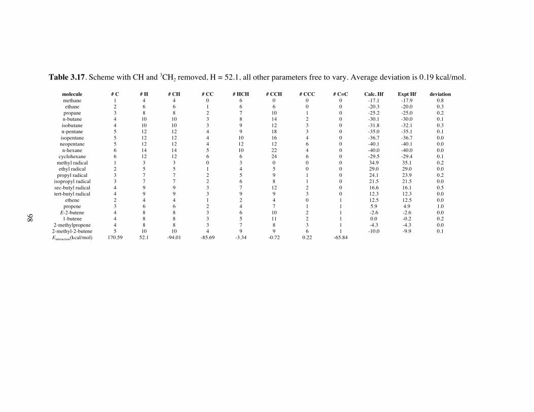
98

Table 3.17. Scheme with CH and 3CH2 removed, H = 52.1, all other parameters free to vary. Average deviation is 0.19 kcal/mol.


methane 1 4 4 0 6 0 0 0 -17.1 -17.9 0.8

ethane 2 6 6 1 6 6 0 0 -20.3 -20.0 0.3

propane 3 8 8 2 7 10 1 0 -25.2 -25.0 0.2

n-butane 4 10 10 3 8 14 2 0 -30.1 -30.0 0.1

isobutane 4 10 10 3 9 12 3 0 -31.8 -32.1 0.3

n-pentane 5 12 12 4 9 18 3 0 -35.0 -35.1 0.1

isopentane 5 12 12 4 10 16 4 0 -36.7 -36.7 0.0

neopentane 5 12 12 4 12 12 6 0 -40.1 -40.1 0.0

n-hexane 6 14 14 5 10 22 4 0 -40.0 -40.0 0.0

cyclohexane 6 12 12 6 6 24 6 0 -29.5 -29.4 0.1

methyl radical 1 3 3 0 3 0 0 0 34.9 35.1 0.2

ethyl radical 2 5 5 1 4 5 0 0 29.0 29.0 0.0

propyl radical 3 7 7 2 5 9 1 0 24.1 23.9 0.2




ethene 2 4 4 1 2 4 0 1 12.5 12.5 0.0

propene 3 6 6 2 4 7 1 1 5.9 4.9 1.0

E-2-butene 4 8 8 3 6 10 2 1 -2.6 -2.6 0.0

1-butene 4 8 8 3 5 11 2 1 0.0 -0.2 0.2

2-methylpropene 4 8 8 3 7 8 3 1 -4.3 -4.3 0.0

2-methyl-2-butene 5 10 10 4 9 9 6 1 -10.0 -9.9 0.1


99

Table 3.18. Scheme with CH and 3CH2 removed, C = 170.6 and H = 52.1, all other parameters free to vary. Average deviation is 0.19

kcal/mol.


methane 1 4 4 0 6 0 0 0 -17.1 -17.9 0.8

ethane 2 6 6 1 6 6 0 0 -20.3 -20.0 0.3

propane 3 8 8 2 7 10 1 0 -25.2 -25.0 0.2

n-butane 4 10 10 3 8 14 2 0 -30.1 -30.0 0.1

isobutane 4 10 10 3 9 12 3 0 -31.8 -32.1 0.3

n-pentane 5 12 12 4 9 18 3 0 -35.0 -35.1 0.1

isopentane 5 12 12 4 10 16 4 0 -36.7 -36.7 0.0

neopentane 5 12 12 4 12 12 6 0 -40.1 -40.1 0.0

n-hexane 6 14 14 5 10 22 4 0 -40.0 -40.0 0.0

cyclohexane 6 12 12 6 6 24 6 0 -29.5 -29.4 0.1

methyl radical 1 3 3 0 3 0 0 0 34.8 35.1 0.3

ethyl radical 2 5 5 1 4 5 0 0 29.0 29.0 0.0

propyl radical 3 7 7 2 5 9 1 0 24.1 23.9 0.2




ethene 2 4 4 1 2 4 0 1 12.5 12.5 0.0

propene 3 6 6 2 4 7 1 1 5.9 4.9 1.0

E-2-butene 4 8 8 3 6 10 2 1 -2.6 -2.6 0.0

1-butene 4 8 8 3 5 11 2 1 0.0 -0.2 0.2

2-methylpropene 4 8 8 3 7 8 3 1 -4.3 -4.3 0.0

2-methyl-2-butene 5 10 10 4 9 9 6 1 -9.9 -9.9 0.0


100

Table 3.19. Scheme with CH and 3CH2 removed, C = 170.6, H = 52.1, CCH = 0.0, CCC = 0.0, all other parameters free to vary.

Average deviation is 0.50 kcal/mol.


methane 1 4 4 0 6 0 0 0 -17.1 -17.9 0.8

ethane 2 6 6 1 6 6 0 0 -20.0 -20.0 0.0

propane 3 8 8 2 7 10 1 0 -24.9 -25.0 0.1

n-butane 4 10 10 3 8 14 2 0 -29.9 -30.0 0.1

isobutane 4 10 10 3 9 12 3 0 -31.8 -32.1 0.3

n-pentane 5 12 12 4 9 18 3 0 -34.8 -35.1 0.3

isopentane 5 12 12 4 10 16 4 0 -36.7 -36.7 0.0

neopentane 5 12 12 4 12 12 6 0 -40.7 -40.1 0.6

n-hexane 6 14 14 5 10 22 4 0 -39.7 -40.0 0.3

cyclohexane 6 12 12 6 6 24 6 0 -29.4 -29.4 0.0

methyl radical 1 3 3 0 3 0 0 0 32.8 35.1 2.3

ethyl radical 2 5 5 1 4 5 0 0 27.9 29.0 1.1

propyl radical 3 7 7 2 5 9 1 0 23.0 23.9 0.9




ethene 2 4 4 1 2 4 0 1 11.4 12.5 1.1

propene 3 6 6 2 4 7 1 1 5.6 4.9 0.7

E-2-butene 4 8 8 3 6 10 2 1 -2.3 -2.6 0.3

1-butene 4 8 8 3 5 11 2 1 -0.3 -0.2 0.1

2-methylpropene 4 8 8 3 7 8 3 1 -4.3 -4.3 0.0

2-methyl-2-butene 5 10 10 4 9 9 6 1 -11.1 -9.9 1.2

Einteraction(kcal/mol) 170.6 52.1 -96.07 -85.59 -1.97 0.0 0.0 -64.34

101

3.9. REFERENCES

[1] H. Y. Afeefy, J. F. Liebman, S. E. Stein, Neutral Thermochemical Data. In NIST

Chemistry Webbook, NIST Standard Reference Database Number 69, P. J. Linstrom,

W. G. Mallard, Eds., National Institute of Standards and Technology: Gaithersburg,

MD (http://webbook.nist.gov).

[2] N. Cohen, S. W. Benson, Chem. Rev. 1993, 93, 2419.


[4] K. Exner, P. v. R. Schleyer, J. Phys. Chem. A 2001, 105, 3407.

[5] For example, correlations have been found in some European countries between

human birth rates and stork populations. We have found many other numerical

combinations of values that give good results when employed in a similar treatment

(data fitting employed the Excel program).


Diego, CA) 2005.



[8] M. D. Wodrich, C. S. Wannere, Y. Mo, P. D. Jarowski, K. N. Houk, P. v. R. Schleyer,

Chem. Eur. J. 2006, to be submitted.

[9] S. J. Blanksby, G. B. Ellison, Acc. Chem. Res. 2003, 36, 255.

CHAPTER 4

SYSTEMATIC ERRORS IN COMPUTED ALKANE ENERGIES USING B3LYP AND

OTHER POPULAR DFT FUNCTIONALS†

† Matthew D. Wodrich, Clémence Corminboeuf, and Paul von Ragué Schleyer. Organic

Letters 2006, 8, 3631. Copyright 2006 American Chemical Society.

103

4.1. ABSTRACT

Energies computed by B3LYP and other popular DFT functionals are flawed by

systematic errors, which can become considerable for larger molecules. These errors,

predominantly due to inadequacies in assessing longer-range non-bonded attractive

effects (dispersion), are illustrated by the isodesmic stabilization energies of n-alkanes

(based on methane and ethane, which have no stabilizing 1,3-alkyl group interactions).

Newer functionals, designed to describe weak interactions, give somewhat better

agreement with experiment, but are not fully satisfactory.

4.2. INTRODUCTION

Kohn-Sham density functional theory has become the standard computational chemistry

method. Based on its superior performance in numerous energy assessments of small

molecules, B3LYP is the most widely used functional. B3LYP reproduces the geometries

of smaller and larger molecules very well. Despite such successes, there is increasing

awareness that B3LYP can fail badly in describing the energies of van der Waals

molecules, hydrogen bonded systems, reaction barrier heights, and larger molecules.[1-4]

B3LYP computations of even the most basic organic molecules, the n-alkanes, result in

systematic errors in the predicted heats of formation[5-8] and bond energies.[9-12] Redfern et

al.[13] reported increasing deviations between B3LYP and G3 theory as the n-alkane chain

is lengthened (Figure 1). Errors in B3LYP computations of experimental homolytic C–C

bond breaking energies of methyl-substituted ethanes and the relative stabilities of

isomers become more serious as the molecules become larger.[14-16] The “cumulative

effect of the errors in large molecules”[7] “discourage the use of the B3LYP model for

104

reaction energy calculations of organic compounds containing more than four carbon

atoms.”[14] Possible origins of these shortcomings (e.g., dispersion) have been

considered,[14,16] but the problems have not been overcome.

Figure 4.1. Error per bond in calculated enthalpies of formation for n-alkanes.

Reproduced from Reference 4.

We computed the isodesmic stabilization energies (Equation 1) of the linear

conformations of the n-alkanes in order to assess and to help understand the errors given

by numerous early and more recent DFT functionals. Figure 2 compares the results

against the experimental data and emphasizes the poor performance of most of the

functionals with these basic organic molecules.

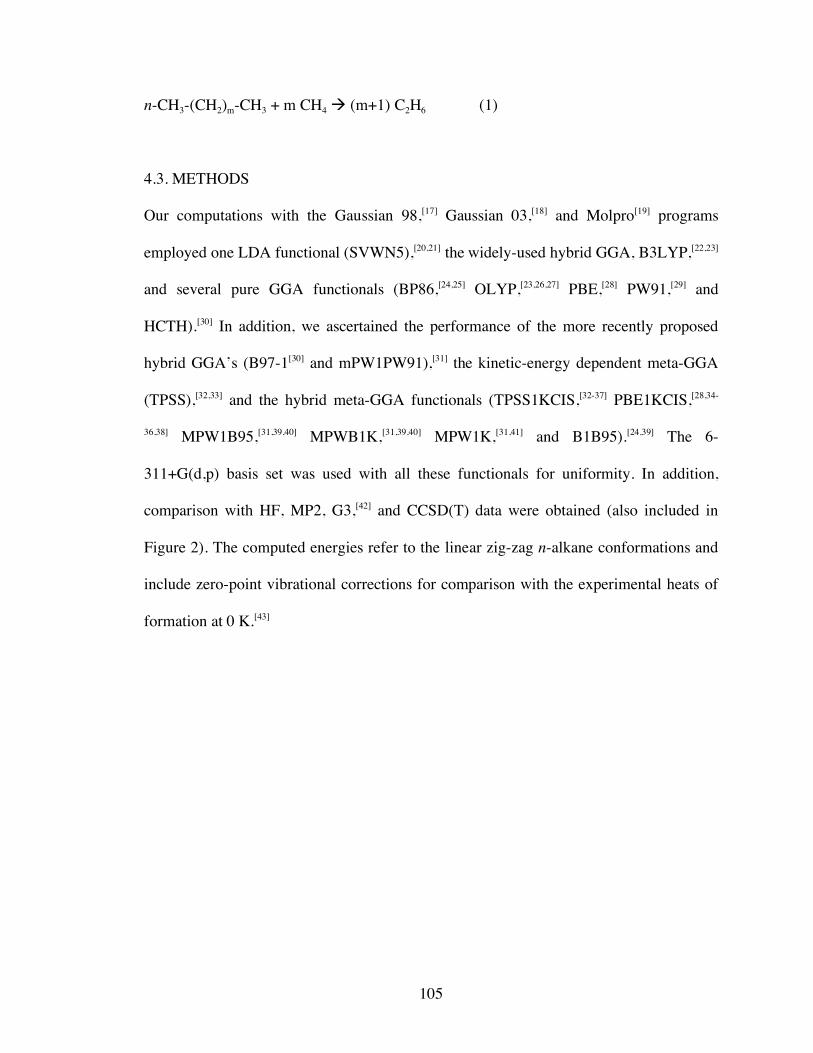
105

n-CH3-(CH2)m-CH3 + m CH4 ! (m+1) C2H6 (1)

4.3. METHODS

Our computations with the Gaussian 98,[17] Gaussian 03,[18] and Molpro[19] programs

employed one LDA functional (SVWN5),[20,21] the widely-used hybrid GGA, B3LYP,[22,23]

and several pure GGA functionals (BP86,[24,25] OLYP,[23,26,27] PBE,[28] PW91,[29] and

HCTH).[30] In addition, we ascertained the performance of the more recently proposed

hybrid GGA’s (B97-1[30] and mPW1PW91),[31] the kinetic-energy dependent meta-GGA

(TPSS),[32,33] and the hybrid meta-GGA functionals (TPSS1KCIS,[32-37] PBE1KCIS,[28,34-

36,38] MPW1B95,[31,39,40] MPWB1K,[31,39,40] MPW1K,[31,41] and B1B95).[24,39] The 6-

311+G(d,p) basis set was used with all these functionals for uniformity. In addition,

comparison with HF, MP2, G3,[42] and CCSD(T) data were obtained (also included in

Figure 2). The computed energies refer to the linear zig-zag n-alkane conformations and

include zero-point vibrational corrections for comparison with the experimental heats of

formation at 0 K.[43]

106

4.4. RESULTS AND DISCUSSION

Figure 4.2. Deviations of various DFT functionals from experimental (0 K)

protobranching stabilization energies. Negative values denote underestimation.

Stabilization energies are based on Equation 1. CCSD(T) and MP2 refer to

CCSD(T)/aug-cc-pVTZ//MP2/6-311+G(d,p) and MP2/aug-cc-pVTZ//MP2/6-

311+G(d,p), respectively, and include MP2/6-311+G(d,p) zero-point corrections. All

other computations employed the 6-311+G(d,p) basis set .

We attribute the increasingly large discrepancies between the computed and

experimental energies apparent in Figures 1 and 2 to “protobranching.”[44-46]

Protobranching, defined as the stabilizing interactions between two 1,3-disposed methyl

(or methylene) groups in propane, higher linear, and branched alkanes, offers new insight

into hydrocarbon stabilization. Each homologation of linear alkanes results in a further

stabilization of ca. 2.8 kcal/mol, relative to methane and ethane (evaluated using Pople’s

107

isodesmic bond energy (BSE) separation reaction, Eq. 1,[47-49] where m also gives the

number of protobranches). Topologically branched alkanes like isobutane and neopentane

have more protobranches and are stabilized to an even larger extent than linear alkanes.[44-

46] These 1,3 stabilizations between geminal groups can be attributed predominantly to

attractive intramolecular van der Waals interactions arising from London dispersion

forces[50,51] (i.e. long range R-6 electron correlation effects). However, Grimme’s[16] very

recent analysis points instead to the greater importance of medium-range electron

correlation differences. Hartree-Fock (HF), B3LYP, and many other functionals give

unsatisfactory results (Figure 1 and 2) since they strongly underestimate the 1,3

stabilization effects.

The Hartree-Fock approximation completely neglects dynamic electron

correlation. B3LYP as well as most well-established density functionals only use local

electron densities to describe correlation and do not account for medium[16] and longer-

range dispersion interactions.[52] However, the design of DFT functionals that perform

well for weak interactions is the goal of much current research.[16,38,53-56] DFT energies are

affected by additional sources of error. For instance, correlation functionals that eliminate

the “self-exchange” problem are being sought.[39] This error (not shared by Hartree-Fock),

arises from the spurious interaction of an electron with itself.

Nearly all the DFT functionals systematically underestimate the energies of n-

alkane chains (Figure 2). Shockingly, the widely used B3LYP is among the worst

functionals and underestimates each protobranching stabilization by 1.33 kcal/mol on

average. Note that this 40% underestimation is comparable to the 47% of HF. OLYP, the

poorest performer in our set, underestimates the stabilization energy by 1.8 kcal/mol on

108

average. Indeed, the exchange functional for OLYP was fit with a restricted set of data

which lacked weakly bonded systems.[27] Other functionals, including the non-empirical

TPSS meta-GGA, and the semi-empirical HCTH GGA underestimate branching, their

mean absolute deviations (MAD) range from 1.10 to 1.50 kcal/mol. Although the LDA

approximation generally strongly overestimates weak interaction energies,[5,57-59] SVWN5

performs best here (Figure 2). Similarly small errors have been reported before for

propane, butane, and isobutane, provided that error-cancelling isodesmic evaluations (cf.,

Equation 1) were employed.[7] Of course, caution must be exercised because of the well

documented deficiencies of LDA.[5,7,52]

The PW91 and the closely related “parameter-free” PBE exchange correlation

GGA functionals describe the binding in attractive van der Waals regions more

accurately;[60] their MADs are 1.05 and 1.08 kcal/mol, respectively, per protobranch.

Somewhat better results are given by the recently developed hybrid meta-GGAs,

MPW1B95 and MPW1B1K of Zhao and Truhlar, designed partially for the description of

weakly interacting systems.[53] Not surprisingly, these new functionals outperform

B3LYP and other early functionals. However, signicant errors (which are cumulative,

Figure 2) still remain.

Unlike DFT, both MP2 and CCSD(T) results depend on basis set size.[61] The

expected overestimation[62-64] of the branching stabilization is found at MP2/aug-cc-

pVTZ, but not at the lower MP2/6-311+G(d,p) level. This suggests the possible existance

of an intramolecular basis set superposition error. Similarly, CCSD(T)/6-311+G(d,p)

results diverge somewhat from experiment but aug-cc-pVTZ values parallel those of

109

experiment. Obviously, computational expense precludes application to longer n-alkane

chains.

Figure 2 emphasizes the regularity of the increasingly large deviations from the

experimental BSE stabilizations as the n-alkane chain is lengthened. Check and Gilbert[14]

also noted regularities in the computed bond dissociation energies of the central C-C

bond of ethane as the number of methyl substituents increases. The B3LYP error

increases to 21.1 kcal/mol for 2,2,3,3-tetramethylbutane; its high degree of branching

enhances the long-range attractions. B3LYP fails as a consequence. Indeed, most of the

functionals in Figure 2 systematically underestimate weak long-range interactions. Their

poor performance appears to arise principally from their inadequacies in accounting for

long and medium-range electron correlation effects.[16]

The adjacent paper by Schreiner et al.[15] illustrates the problems in reproducing

the experimental relative energies of hydrocarbons, especially when isomers having a

different blend of single and multiple CC bonds are compared, at various DFT and ab

initio levels. The preferred geometries of [n]annulenes were found earlier to depend

strongly on the level of theory employed.[65]

Curtiss, et al.[7] have noted that homodesmotic energy evaluations improve the

accuracy of B3LYP for large molecules. However, for alkanes this only arises through

cancellation of the protobranching errors (Equation 2, where m also is the number of

protobranches).

CH3-(CH2)m-CH3 + (m-1) C2H6 ! m C3H8 (2)

110

Linear and branched alkanes larger than ethane are stabilized by intramolecular

1,3 “protobranching” interactions between alkyl groups. The most commonly used DFT

functionals, notably B3LYP, underestimate the protobranching stabilization mainly due

to their inadequate descriptions of long-range non-bonded interactions. We join with

others[15] to discourage the use of B3LYP energy data for larger molecules.

Unfortunately, the DFT alternatives are only somewhat better, but are not yet fully

satisfactory.

The recent hybrid meta-GGA functionals of Zhao and Truhlar, as well as other

recently proposed van der Waals-corrected DFT functionals[53-56] with the correct R-6

asymptotic behavior, may provide more accurate assessments of weakly-bound systems

and better descriptions of intramolecular non-bonded interactions at considerably less

computational cost than post-HF wavefunction methods. However, even the best-

performing MPW1B95 and MPWB1K hybrid meta-GGA functionals[31,39,40] do not

evaluate the energies of n-alkane chains accurately, and only offer some improvement

over B3LYP for larger molecules. We hope that Check and Gilbert’s pessimistic

admonition, “a computational chemist cannot trust a one-type DFT calculation”[14] can be

overcome eventually.

111

4.5. ACKNOWLEDGMENTS

We thank Y. Bernard (University of Geneva) and N. L. Allinger (University of Georgia)

for helpful comments, J. M. Turney and H. F. Schaefer III (University of Georgia) for

computational resources, as well as the authors of ref. 15 for sharing their results prior to

publication. The Petroleum Research Fund and NSF Grant CHE-0209857 supported our

work.

112

4.6 REFERENCES

[1] B. J. Lynch, P. L. Fast, M. Harris, D. G. Truhlar, J. Phys. Chem. A 2000, 104, 4811.

[2] Y. Zhao, O. Tishchenko, D. G. Truhlar, J. Phys. Chem. B 2005, 109, 19046.

[3] S. Tsuzuki, H. P. Luthi, J. Chem. Phys. 2001, 114, 3949.

[4] J. A. Duncan, M. C. Spong, J. Phys. Org. Chem. 2005, 18, 462.

[5] K. Raghavachari, B. B. Stefanov, L. A. Curtiss, Mol. Phys. 1997, 91, 555.

[6] L. A. Curtiss, K. Raghavachari, P. C. Redfern, J. A. Pople, J. Chem. Phys. 1997, 106,

1063.

[7] L. A. Curtiss, K. Raghavachari, P. C. Redfern, J. A. Pople, J. Chem. Phys. 2000, 112,

7374.

[8] M. Saeys, M.-F. Reyniers, G. B. Marin, V. van Speybroeck, J. Waroquier, J. Phys.

Chem. A 2003, 107, 9147.

[9] Y. Feng, L. Liu, J.-T. Wang, H. Huang, Q.-X. Guo, J. Chem. Inf. Comput. Sci. 2003,

43, 2005.

[10] Y. Fu, X. Y. Dong, Y. M. Wang, L. Liu, Q.-X. Guo, Chin. J. Chem. 2005, 23, 474.

[11] M. L. Coote, A. Pross, L. Radom in Fundamental World of Quantum Chemistry,

Vol. III Eds.: E. J. Brandas and E. S. Kryachko), Kluwer Academic Publishers, The

Netherlands, 2004, p. 563.

[12] E. I. Izgorodina, M. L. Coote, L. Radom, J. Phys. Chem. A 2005, 109, 7558.

113

[13] P. C. Redfern, P. Zapol, K. Raghavachari, L. A. Curtiss, J. Phys. Chem. A 2000, 104,

5850.

[14] C. E. Check, T. M. Gilbert, J. Org. Chem. 2005, 70, 9828.

[15] P. R. Schreiner, A. A. Fokin, R. A. Pascal, Jr. , A. de Meijere, Org. Lett. 2006, 8,

3635.

[16] S. Grimme, Angew. Chem. Int. Ed. 2006, 45, 4460.











[18] Gaussian 03, Revision C.02, M. J. Frisch, G. W. Trucks, H. B. Schlegel, G. E.

Scuseria, M. A. Robb, J. R. Cheeseman, J. A. Montgomery, Jr., T. Vreven, K. N. Kudin,

J. C. Burant, J. M. Millam, S. S. Iyengar, J. Tomasi, V. Barone, B. Mennucci, M. Cossi,

G. Scalmani, N. Rega, G. A. Petersson, H. Nakatsuji, M. Hada, M. Ehara, K. Toyota, R.

114

Fukuda, J. Hasegawa, M. Ishida, T. Nakajima, Y. Honda, O. Kitao, H. Nakai, M. Klene,

X. Li, J. E. Knox, H. P. Hratchian, J. B. Cross, V. Bakken, C. Adamo, J. Jaramillo, R.

Gomperts, R. E. Stratmann, O. Yazyev, A. J. Austin, R. Cammi, C. Pomelli, J. W.

Ochterski, P. Y. Ayala, K. Morokuma, G. A. Voth, P. Salvador, J. J. Dannenberg, V. G.

Zakrzewski, S. Dapprich, A. D. Daniels, M. C. Strain, O. Farkas, D. K. Malick, A. D.

Rabuck, K. Raghavachari, J. B. Foresman, J. V. Ortiz, Q. Cui, A. G. Baboul, S. Clifford,

J. Cioslowski, B. B. Stefanov, G. Liu, A. Liashenko, P. Piskorz, I. Komaromi, R. L.

Martin, D. J. Fox, T. Keith, M. A. Al-Laham, C. Y. Peng, A. Nanayakkara, M.

Challacombe, P. M. W. Gill, B. Johnson, W. Chen, M. W. Wong, C. Gonzalez, and J. A.

Pople, Gaussian, Inc., Wallingford CT, 2004.

[19] MOLPRO, a package of ab initio programs designed by J.-J. Werner, P. J. Knowles,

version 2002.1, contributed by R. D. Amos, A. Bernhardsson, A. Berning, et al.

[20] S. H. Vosko, L. Wilk, M. Nusair, Can. J. Phys. 1980, 58, 1200.

[21] J. C. Slater, Quantum Theory of Molecular Solids: The Self-Consistent Field for

Molecules and Solids, McGraw-Hill, New York, 1974.

[22] A. D. Becke, J. Chem. Phys. 1993, 98, 5648.




[26] N. C. Handy, A. J. Cohen, Mol. Phys. 2001, 99, 403.

115

[27] W. M. Hoe, A. J. Cohen, N. C. Handy, Chem. Phys. Lett. 2001, 341, 319.




[30] F. A. Hamprecht, A. J. Cohen, D. J. Tozer, N. C. Handy, J. Chem. Phys. 1998, 109,

6264.

[31] C. Adamo, V. Barone, J. Chem. Phys. 1998, 108, 664.

[32] V. N. Staroverov, G. E. Scuseria, J. Tao, J. P. Perdew, J. Chem. Phys. 2003, 119,

12129.

[33] J. Tao, J. P. Perdew, V. N. Staroverov, G. E. Scuseria, Phys. Rev. Lett. 2003, 91,

146401.

[34] J. Rey, A. Savin, Int. J. Quantum Chem. 1998, 69, 581.

[35] J. B. Krieger, J. Chen, G. J. Iafrate, A. Savin in Electron Correlations and Materials

Properties, Vol. Eds.: A. Gonis and N. Kioussis), Plenum, New York, 1999, p. 463.

[36] J. Toulouse, A. Savin, C. Adamo, J. Chem. Phys. 2002, 117, 10465.

[37] Y. Zhao, B. J. Lynch, D. G. Truhlar, Phys. Chem. Chem. Phys. 2005, 7, 43.

[38] Y. Zhao, D. G. Truhlar, J. Chem. Theory Comput. 2005, 1, 415.


116

[40] Y. Zhao, D. G. Truhlar, J. Phys. Chem. A 2004, 108, 6908.


[42] L. A. Curtiss, P. C. Redfern, K. Raghavachari, V. Rassolov, J. A. Pople, J. Chem.

Phys. 1999, 110, 4703.

[43] NIST Computational Chemistry Comparison and Benchmark Database, NIST

Standard Reference Database Number 101 Release 12, Aug 2005, Editor: Russell D.

Johnson III http://srdata.nist.gov/cccbdb.

[44] M. D. Wodrich, C. S. Wannere, Y. Mo, P. D. Jarowski, K. N. Houk, P. v. R.

Schleyer, Chem. Eur. J. 2006, to be submitted.


Diego, CA) 2005.



[47] W. J. Hehre, R. Ditchfield, L. Radom, J. A. Pople, J. Am. Chem. Soc. 1970, 92,

4796.

[48] L. Radom, W. J. Hehre, J. A. Pople, J. Am. Chem. Soc. 1971, 93, 289.

[49] W. J. Hehre, L. Radom, P. v. R. Schleyer, J. A. Pople, Ab Initio Molecular Orbital

Theory, John Wiley & Sons, New York, 1986.

[50] K. S. Pitzer, E. Catalano, J. Am. Chem. Soc. 1956, 78, 4844.

117

[51] K. S. Pitzer, Adv. Chem. Phys. 1959, 2, 59.

[52] W. Koch, M. C. Holthausen, A Chemist's Guide to Density Functional Theory,

Wiley-VCH, Weinheim, 2001.

[53] X. Wu, M. C. Vargas, S. Nayak, V. Lotrich, G. Scoles, J. Chem. Phys. 2001, 115,

8748.

[54] U. Zimmerli, M. Parrinello, P. Koumoutsakos, J. Chem. Phys. 2004, 120, 2693.

[55] O. A. von Lilienfeld, I. Tavernelli, U. Rothlisberger, D. Sebastiani, Phys. Rev. Lett.

2004, 93, 153004.

[56] T. Sato, T. Tsuneda, K. Hirao, Mol. Phys. 2005, 103, 1151.

[57] L. Zhechkov, T. Heine, S. Patchkovskii, G. Seifert, H. A. Duarte, J. Chem. Theory

Comput. 2005, 1, 841.

[58] M. Lein, J. F. Dobson, E. K. U. Gross, J. Comput. Chem. 1999, 20, 12.

[59] H. Valdes, J. A. Sordo, J. Comput. Chem. 2002, 23, 444.

[60] Y. K. Zhang, W. Pan, W. T. Yang, J. Chem. Phys. 1997, 107, 7921.

[61] The BSE for propane changes by only 0.07 kcal/mol in going from B3LYP/6-

311+G(d,p) to B3LYP/cc-pVTZ.

[62] S. Grimme, J. Comput. Chem. 2004, 25, 1463.

118

[63] S. Tsuzuki, T. Uchimaru, K. Matsumara, M. Mikami, K. Tanabe, Chem. Phys. Lett.

2000, 319, 547.

[64] P. Hobza, H. L. Selzle, E. W. Schlag, J. Phys. Chem. 1996, 100, 18790.

[65] C. S. Wannere, K. W. Sattelmeyer, H. F. Schaefer, P. v. R. Schleyer, Angew. Chem.

Int. Ed. 2004, 43, 4296.

CHAPTER 5

AROMATICITY AND DOUBLE AROMATICITY IN MONOCYLIC BORON,

CARBON, AND BOROCARBON COMPOUNDS†

† Matthew D. Wodrich, Clémence Corminboeuf, Sung Soo Park and Paul von Ragué Schleyer. To be submitted to Chemistry – A European Journal.

120

5.1 ABSTRACT

The double aromatic character of selected monocyclic carbon, boron, and borocarbon

rings is demonstrated by refined nucleus-independent chemical shift (NICS) analyses

involving the contributions of individual canonical MOs and their out-of-plane NICS

tensor component (CMO-NICSzz). Double aromaticity results from two mutually

orthogonal Hückel p AO frameworks in a single molecule. The familiar ! orbitals are

augmented by the in-plane delocalization of electrons occupying sets of radial p orbitals.

Such double aromaticity is present in C6H3+, C6

4+, C4B44+, C6, C5B2, C4B4, C2B8, B10

2-, B12,

C10, C9B2, C8B4, C7B6, C6B8, and C14. Monocyclic C8 and C12 are doubly anti-aromatic,

since both the orthogonal ! and radial Hückel sets are paratropic. Planar C7 and C9

monocycles have mixed ! aromatic/radial antiaromatic systems.

5.2 INTRODUCTION

Double aromaticity,[1] as originally conceived by Chandrasekhar, Jemmis, and Schleyer in

1979, is defined as the existence of two mutually orthogonal Hückel framework MO sets

in a single molecule. Both of these orthogonal systems can stabilize molecules. The usual

4n+2 ! electron system perpendicular to the plane is augmented by an in-plane 4n+2

electron system comprised of radial (inward-pointing) p AO’s. The C6H3+ ion (Figure 5.1)

provided the first theoretical evidence for double aromaticity; it benefits from having 6!

electrons as well as from the in-plane 3-center-2-electron interaction of the three radial p

atomic orbitals on the bare 1,3, and 5 carbon atoms. Nelson and Kentäamaa’s mass

spectral experiments have identified this species.[2] The C6H3+ ion[3] opened the fields of

121

double and in-plane aromaticity, concepts that have received significant theoretical

attention since.[3-23]

Figure 5.1. The planar C6H3+ doubly aromatic ion comprised of 6! electrons and 2 radial

in-plane electrons.

Further early examples of double aromaticity included C10H5- (10! + 6 rad) and

C8H4 (10! + 2 rad) (Figure 5.2).[3] More recently, Schleyer et al.,[24] analyzed the

structures and magnetic properties of 3,5-dehydrophenyl cation and the closely related

cyclo[6]carbon (C6) in greater detail. The six membered rings of both species had equal

CC bond lengths,[25-27] and enhanced magnetic susceptibility anisotropy.

Figure 5.2. Double aromatic structures of C10H5- (10! + 6 rad) and C8H4 (10! + 2 rad).

122

Carbon clusters have been extensively studied experimentally,[28-42] particularly

those larger clusters serving as precursors to fullerenes and nanotubes.[43-45] Several mass

spectrometry studies have shown the presence of “magic peaks”, which appear as above

average abundances for certain stoichiometries. Photoelectron spectra of monocyclic Cn-

have also shown clear differences between clusters with n=4N and 4N+2 carbon atoms

respectively.[46-48] Such distinctive patterns likely suggest certain stoichiometric structures

to have an enhanced stability.

Along with extensive experimental studies of carbon clusters, many theoretical

calculations probing electronic properties and structures have been made, originating

with Pitzer and Clementi.[49] Using a refined Hückel p-electron model, they predicted that

Cn clusters would be linear and that rings might be formed around n=10. In 1966, these

predictions were corroborated by Hoffmann’s extended Hückel theory.[50] Another

significant paper appeared in 1977, in which Slanina and Zahradnik considered both

linear and cyclic geometries of Cn (n = 4-7) clusters using Dewar et al.’s MINDO/2

method.[51] This first comprehensive examination of structures indicated that 3-

dimensional and monocyclic were nearly always preferred over linear species. In the

middle 1970’s, the Schleyer-Pople group was also interested in the possibility that rings

with 4N+2 carbons might be “doubly aromatic,” stabilized by both perpendicular and in-

plane Hückel systems, but the limited computational resources of the day (E. M. Engler,

at IBM, did succeed in computing C10 at STO-3G)[52] did not permit reliable tests and

developments of this idea using ab initio methods. Since then, extensive ab initio studies

have confirmed that an energetic competition exists between linear (triplet) and cyclic

(singlet) isomers of medium-size Cn clusters.[53] Most recent theoretical analysis have

123

shown that the monocyclic C6 and C10 singlet states are lower in energy than their linear

counterparts.[12,28,53-65] Interestingly, the lowest energy structures for C6 and C10 correspond

to the bond angle alternating polyallene D3h and D5h rather than the full D6h and D10h

symmetry (equal bond lengths and angles), which are transition states. Despite a sizable

HOMO-LUMO gap, the symmetry of their frontier molecular orbitals allows for a

second-order Jahn-Teller distortion.[13,66,67] Alternatively, rings with 4N carbon atoms

generally display a strong first-order Jahn-Teller distortion leading to C2nh polyynic

structures[61,65,68] which are doubly antiaromatic according to the Hückel rule. However,

the question has been raised whether it is possible for a formally doubly antiaromatic

molecule (4n+4m) to become doubly aromatic by using alternative electronic

configurations with 4n+2 and 4m-2 electrons in the two orthogonal frameworks.[1]

Boron, as well as borocarbons (a binary compounds comprised only of boron and

carbon atoms), constitute other classes of related molecules. Unlike carbon clusters,

borocarbons have received remarkably little attention as a class, despite several examples

of remarkable structures.[69-73] Three C3B4 isomers, for example, have planar

hexacoordinate carbons.[73] In contrast, binary combinations of carbon with lithium,

nitrogen, oxygen, fluorine and other main group elements have been studied in detail.

Boron carbide,[74-86] one of the hardest materials known, having a number of important

uses, has received the most attention. Diatomic and larger BC clusters have been studied

using mass spectrometry[87,88] and EPR.[89-91] Other studies have probed the structure of

BnCm (n+m = 2-5) clusters.[92-101] Park[102] described structural and bonding trends in a

series of isoelectronic borocarbon compounds. Potential energy surface investigations

reveal that the global isomers of B7C11-, B6C2, and B5C3

1+ all prefer monocyclic rings

124

surrounding a heptacoordinate boron atom. Many other borocarbons have been found

computationally to have planar terta-, penta-, and hexa-coordinate carbon

structures.[69,70,73,103-107]

Further analysis of molecular properties allows for the corroboration of electron

delocalization in orthogonal planes within these structures. Recently, Martín-Santamaría

and Rzepa[14] studied double aromaticity and double anti-aromaticity in small carbon

rings using nucleus-independent chemical shifts (NICS). Introduced in 1996 by Schleyer

et al.,[108] NICS provides a simple and effective magnetic aromaticity index; negative

(diatropic) NICS values (usually depicted by red dots) indicate magnetic aromaticity,

while positive (paratropic) values (green dots) indicate magnetic anti-aromaticity.

Typically, the magnetic environments of molecules are probed by computing a number of

NICS points; those designated NICS(0) are computed at the geometric centers of rings

while NICS(1) are computed at 1Å above the geometric center. Using isotropic NICS(0)

calculations, Martín-Santamaría and Rzepa’s results suggested D5h-C10, D7h-C14, 1,6-C8N2,

1,7-C10B2, Cs-quintet C12, C11H2, and bicyclic C19 to be doubly aromatic. Their

conclusions, however, were based only on isotropic NICS values and employed no

dissection to probe the aromaticity of each individual orthogonal Hückel framework. The

bond angle alternating polyallene D5h-C10 has overall aromatic character, but its NICS(0)

= –28.9 is only on par with, not greater than, that of aromatic C2v [10]-annulene (-

28.6).[109] However, if one considers the D10h C10H10, doubly aromatic D5h-C10 is shown to

have a greater isotropic NICS value (-13.2 vs. -28.9, see later discussion). The difference

in the isotropic NICS(0) value is clearly due the in-plane radial 10 electron system

present in D5h-C10 but not in C10H10! In contrast, the NICS(0) value of the polyallene D7h-

125

C14 (-35.6) is much larger than that of both the D2h [14]-annulene (-13.4) and the D14h

C14H14 (-15.8), one could also conclude that the enhanced isotropic NICS(0) value of D7h-

C14 is due to its additional in-plane aromatic system. Hofmann and Berndt[110] established

the double aromaticity of small boron systems, using enhanced NICS values as a

criterion, and determined that the two-electron delocalization was the key to

understanding their unusual structures. Double aromatic molecules were designed with

two in-plane delocalized electrons using anionic B3, neutral B3, and CB2 subunits (Figure

5.3).

Figure 5.3. Double aromatic structures proposed by Hofmann and Berndt. Reproduced from Reference [110] and neutral CB2.

We now employee more refined NICS analyses,[111-114] which allow the clear-cut

assignment of double aromaticity through the analysis of individual MO contributions, to

investigate a number of carbon, boron, and borocarbon rings.

5.3 METHODS

Carbon clusters and more generally sp bond systems are particularly challenging to

model accurately due to their wide range of geometries and the occurrence of single,

126

double (polyallene) and triple bonds (polyacetylene) that results in a pronounced

multireference character. The nature of the global minimum and the energy separation

between the linear and cyclic Cn isomers is generally extremely sensitive to the

computational level. Similarly, there has been a considerable discussion in the literature

as to which ring structure: regular polygon or cummulenic (equal bonds, alternating

angle) is the ground state. Despite these potential difficulties, geometries and relative

energies obtained at the density functional levels are in reasonable agreements with high-

order correlation methods (e.g. coupled-cluster expansion),[55,61,63] while MP2 predictions

were found to be qualitatively incorrect.[63] In this paper, structures were optimized using

the B3LYP[115,116] hybrid density functional with the 6-311+G(d) basis set (6-311+G(d,p)

for C6H6, C10H10, C14H14, and C6H3+) using Gaussian 98.[117] Furthermore, comparisons

with available CCSD(T) data are provided. All structures, unless otherwise noted, were

characterized as local minima on the potential energy surface and contained no imaginary

frequencies. NICS points were computed at geometric centers, NICS(0), and 1 Å above,

NICS(1), using the Perdew-Wang-91 exchange-correlation functional[118] with the triple-!

GTO IGLO-III valence basis set using the deMon NMR program.[119] NICS contributions

of individual canonical molecular orbitals (CMO-NICS)[120] were performed at

PW91/IGLO-III using the NBO 5.0 program.[121][122] Because isotropic NICS(0) values at

ring centers do not reflect the “ring current” exclusively, we employed NICSzz (the out-

of-plane component of the NICS tensor), as a superior aromaticity measure due to its

more accurate response to magnetic properties arising only from a magnetic field applied

perpendicular to the molecular plane.[111,112,114,123,124]

127

The carbon, boron, and borocarbon rings selected for study here had two potential

“double aromatic” 4n+2 or “double anti-aromatic” 4n electron Hückel systems (! and in-

plane radial) based on simple electron counting. Two valence electrons of both boron and

carbon are assigned to the " framework. Thus, boron has one and carbon two available

electrons for ! and in-plane radial bonding. While many isomers are possible for each

stoichiometry we have focused our evaluation to those being monocyclic and generally of

higher symmetry.

128

5.4 RESULTS AND DISCUSSION

5.4.1 THE C6H3+ ION

The distorted[66] C6H3+ ion (Figures 5.1 and 5.4), the first hypothesized doubly aromatic

species, was predicted by Chandrasekhar, Jemmis, and Schleyer in 1979[1] and further

confirmed in 1994.[24] We have now reexamined D3h C6H3+ using a combination of NICS,

NICSzz, and CMO-NICSzz to quantify the extent of its aromatic and doubly aromatic

character. Large negative isotropic NICS(0) of -43.2 and NICS(1) (isotropic NICS taken

at 1Å above the ring center) of -20.0 values (Table 5.1) indicate the presence of a

diatropic ring current. The large difference between isotropic NICS(0) and NICS(1)

values is a probable indicator that the system contains a diatropic Hückel system in the

molecular plane. If no diatropic in-plane radial system were present, one would expect

the isotropic NICS(0) and NICS(1) values to be similar (as is the case for benzene

NICS(0)= -7.5, NICS(1)= -9.6). The individual canonical molecular orbital contributions

to NICS (CMO-NICS) as well as each out-of-plane NICS tensor component (CMO-

NICSzz), summarized in Table 5.1 and Figure 5.5, show the presence of a strongly

aromatic 6-electron ! system perpendicular to the molecular plane, NICS! = -32.76 and a

weakly aromatic two electron in-plane radial system, NICSrad = -3.59 (Figure 5.4). The

out-of-plane component of the NICS tensor for the ! system in C6H3+ is slightly weaker

than that of benzene (NICSzz = -36.12, while the NICSradzz contributes an additional -

5.30). The remaining contributions to NICSzz arise from several diatropic low-lying

orbitals, as well as minimal paratropic contributions from tangential orbitals (relative to

C64+ and C4B4

4+, see subsequent paragraph). Thus, one expects C6H3+ to be slightly more

aromatic than benzene based on NICS.

129

Are the C64+ and C4B4

4+ monocycles further examples of “6+2” doubly aromatic

systems, akin to C6H3+? All three possess a single diatropic in-plane radial orbital;

however, the overall aromatic character is dominated by the diatropic 6! electron system,

which are very similar in all three ions (NICS!zz). As a result, the three species have

relatively similar NICSzz values. However, the contradictory behavior of the radialzz and

the total NICSzz remains puzzling: the system with the least negative radialzz value has the

most negative NICSzz (Table 5.1). Such behavior is explained by the paratropicity of a

low-lying tangential orbital, which contributes strongly in C64+ but only weakly in C6H3

+.

Thus despite having a smaller radialzz values, the tangential orbital contribution in C6H3+

(+7.66 ppm) has only a minimal effect on its NICSzz value while the large value of the

C64+ tangential orbital (+24.59 ppm) has considerable impact on its total NICSzz. The end

result is total NICSzz values which contrast the sum of their !zz and radialzz components. It

should be noted, however, that Fowler has shown that low-lying orbitals have little or no

effect on ring currents.[125]

130

Figure 5.4. Geometries, point groups, and isotropic NICS values (red indicates diatropicity while green indicated paratropicity) of carbon clusters.

131

Figure 5.5. CMO-NICS plot of C6H3+. CMO-NICS and CMO-NICSzz contributions are

listed on the right side in ppm; the “Total” listed at the bottom represents the contributions of all orbitals, not just those pictured. MO energies in a.u. are given on the left side.

5.4.2 EVEN NUMBERD CARBON CLUSTER MONOCYCLICS

The most recent theoretical investigations conclude that cyclic C6 prefers D3h symmetry

over both the D6h and the linear chain forms (Figure 5.4).[55,64] This geometrical preference

can be attributed to a second-order Jahn-Teller effect.[66] At the CCSD(T) level, Hutter

and Lüthi[55] predicted the D3h global minimum to lie 8.3 kcal/mol below the regular

hexagon D6h transition state structure and obtained good agreement at the BP86/TZVP

level for both geometries and energies. At the B3LYP/6-311+G(d) level, the

interconversion barrier between the D3h and D6h structures is 13.62 kcal/mol.

The magnetic behavior of the global D3h minimum is peculiar. The out-of-plane

component of the NICS tensor for the ! system (NICS!zz) is slightly larger than that of

benzene, yet the in-plane system is paratropic at the ring center. This suggests that D3h-C6

132

is ! aromatic and radial anti-aromatic. However, a grid of NICSzz points, dissected into !

and radial contributions, shows a clear change from paratropic within the central triangle

to diatropic within the outer triangles and, as expected for aromatic systems, a

deshielding zone outside the molecular framework (Figure 5.6). A possible explanation

for this peculiar behavior is the presence of local diatropic ring currents within the three

outer triangles, which necessarily causes the central triangle to be paratropic (Figure 5.7).

Alternatively, similar paratropic NICSradzz patterns are observed at the center of

cyclopropane and, more generally, at the center of six "-electrons D3h aromatic rings.[126]

Akin to this set of "-aromatic D3h three membered rings, the paratropic shielding at the

center of D3h-C6 arises essentially from the degenerate set of HOMOs with Möbius

topology, as shown in Figure 5.8. While further analysis on this seemingly pathological

NICS behavior are impending, the computation of isotropic NICS(0), or even dissected

NICS grids at several points is strongly recommended when determining the overall

magnetic character of atypical molecules. The NICSzz grid suggests that the D3h structure

of C6 is doubly aromatic.

133

Figure 5.6. NICS!zz and NICSradzz grids of C6 (D3h and D6h). The NICS

!zz grids indicate the ! systems to be diatropic within the molecular framework while the NICSradzz grids indicates the radial system is paratropic in the central triangle and diatropic in the outer triangles for D3h and diatropic throughout for D6h.

134

Figure 5.7. Proposed ring current model for the radial system of D3h C6.

Although being a transition state, we have investigated the magnetic properties of

the regular D6h-C6 structure. The isotropic NICS(0) value of D6h-C6 (–36.9) is appreciably

larger than the –25.1 NICS(0) D3h-C6 (Table 5.1). Since archetype aromatic molecules

generally exhibit special thermodynamic stability and a diatropic ring current, the

enhanced diatropicity of the less stable D6h structure appears surprising. However, several

studies indicate that different aromaticity measures may provide divergent

information.[113,127] For instance, the lowest energy fused heterobicycles are not the most

aromatic isomers.[128] In addition, the differences in diatropicity of the D6h and D3h

structures are less pronounced when considering larger shielding zones. The NICSzz grids

shown in Figure 5.6, clearly illustrate the overall diatropicity of both the D3h and D6h

structures.

135

Figure 5.8. D6h (A) and D3h (B) CMO-NICS plots of C6. CMO-NICS and CMO-NICSzz contributions are listed on the right side in ppm; the “Total” listed at the bottom represents the contributions of all orbitals, not just those pictured. MO energies in a.u. are given on the left side.

Akin to C6, the C10 molecule has long been recognized to adopt a D5h symmetry

(vide supra) which is favored by several tens of kcal mol-1 over the lowest energy linear

isomer (Figure 5.9).[53,58] The equivalent D5h minima interconvert across the transition

state of D10h symmetry, corresponding to an energy barrier of about 1.0 kcal mol-1 at the

CCSD(T)/cc-pVTZ level.[61] Similarly, B3LYP/6-311+G(d) optimization result in a

polyacetylene D5h-C10 stationary point with an interconversion barrier of about 2.5

kcal/mol, which demonstrates the floppy nature of these sp-carbon cluster. While C4n+2

clusters larger than C10 have been studied at less accurate theoretical levels, measured

electronic spectra[129] suggest these structures to be monocyclic rings, which likely exhibit

double aromaticity. At the B3LYP/6-311+G(d) level, the D14h-C14 transition state is

roughly isoenergetic with the D7h cumulenic energy minimum.

136

NICS!zz of both C10 and C14 are similar to those of their parent annulenes[130] (i.e.

C10H10 and C14H14), but their enhanced total NICSzz indicate the presence of an additional

diatropic subsystem. CMO-NICS and CMO-NICSzz analysis indeed confirm that both

carbon monocyclics are doubly aromatic, as has been previously hypothesized.[13,14] Note

the ! MOs of both Cn and CnHn (n=10,14) systems contribute nearly equally, thus the

NICS!zz values for both Cn and CnHn are nearly identical. However, C10 and C14 also

contain a diatropic in-plane radial system, thus their total NICSzz is much greater (>30

ppm) than that of their annulene analogues (Table 5.1).

Figure 5.9. B3LYP/6-311+G(d) optimized bond angles of polyallene D5h C10 and D7h C14.

C8 is an interesting example of a double antiaromatic polyynic ring,[53,54,57,61,68]

possessing orthogonal “8 radial + 8 !” electron systems (Figure 4). CCSD(T)/cc-pVDZ

calculations predict the C4h cyclic form to lie only 4 kcal mol-1 below the linear

structure.[61] Alternatively, Hutter and Luthi identified a boat-like non-planar D4d structure

as a minimum.[60] The energy difference between these two structures is less than 1

kcal/mol s at the B3LYP/aug-cc-PVTZ level[54] once again reflecting the very floppy

nature of these systems. At the PW91/IGLO-III//B3LYP/6-311+G(d) level, both the C4h

137

and D4d minima have small HOMO-LUMO energy separation (only 1.21 eV) resulting in

a large paratropic HOMO-NICS (see SI for the D4d structure).[131] As expected, the highest

lying ! MO (the HOMO), and the highest in-plane radial orbital (HOMO-1), dominate

the overall molecular paratropicity (Figure 5.10). The HOMO-NICS contribution +60.70

(+186.58 HOMO-NICSzz) is very large, while the highest lying occupied orbital of the in-

plane radial system also is strongly paratropic (CMO-NICS +16.47, CMO-NICSzz

+45.09). Not surprisingly, C8 has a smaller ionization potential than C6 or C10.[132] The

polyynic C6h ring was found to be lower in energy than the other C12 isomers at several

DFT levels. However, uncertainties as to which structure is the minimum at higher

theoretical levels remain.[62] Regardless of the relative energies, the C6h ring structure

exhibits the same double antiaromatic character as C8 (see Figure 5.11 and Table 5.1), no

electronic rearrangement to a double aromatic configuration (4n+2, 4m-2) is seen.

138

Figure 5.10. CMO-NICS and CMO-NICSzz of doubly anti-aromatic C8. CMO-NICS and CMO-NICSzz contributions are listed on the right side in ppm; the “Total” listed at the bottom represents the contributions of all orbitals, not just those pictured. MO energies in a.u. are given on the left side.

139

Figure 5.11. CMO-NICS and CMO-NICSzz of doubly antiaromatic C12. CMO-NICS and CMO-NICSzz contributions are listed on the right side in ppm; the “Total” listed at the bottom represents the contributions of all orbitals, not just those pictured. MO energies in a.u. are given on the left side.

5.4.3 ODD NUMBERED CARBON CLUSTER MONOCYCLICS

Martin et al.[63] showed, using DFT and CCSD(T) calculations, that small monocyclic

rings containing odd numbers of carbon atoms (Cn, n=5-9) are higher in energy than the

corresponding linear structures. However, experimental evidence for cyclic C7+ exists[36]

and small linear-cyclic isomerization energy (< 15 kcal mol-1 at the CCSD(T) level) have

been computed for C7 and C9.[63] The ! and radial electron counts of such “odd carbon”

monocycles are not easy to assign a priory. Mixed aromatic/anti-aromatic electronic

structures are possibilities. Cyclic C7 and C9 prefer C2v over planar structures at both the

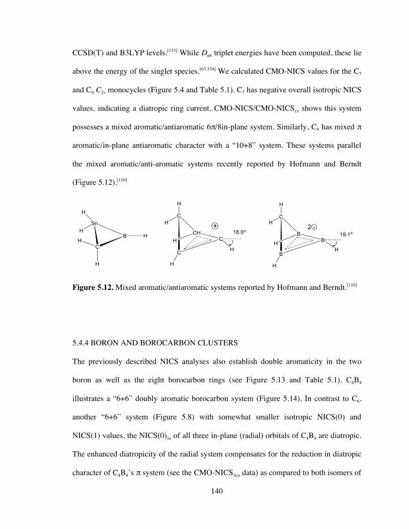
140

CCSD(T) and B3LYP levels.[133] While Dnh triplet energies have been computed, these lie

above the energy of the singlet species.[63,134] We calculated CMO-NICS values for the C7

and C9 C2v monocycles (Figure 5.4 and Table 5.1). C7 has negative overall isotropic NICS

values, indicating a diatropic ring current. CMO-NICS/CMO-NICSzz shows this system

possesses a mixed aromatic/antiaromatic 6!/8in-plane system. Similarly, C9 has mixed !

aromatic/in-plane antiaromatic character with a “10+8” system. These systems parallel

the mixed aromatic/anti-aromatic systems recently reported by Hofmann and Berndt

(Figure 5.12).[110]

Figure 5.12. Mixed aromatic/antiaromatic systems reported by Hofmann and Berndt.[110]

5.4.4 BORON AND BOROCARBON CLUSTERS

The previously described NICS analyses also establish double aromaticity in the two

boron as well as the eight borocarbon rings (see Figure 5.13 and Table 5.1). C4B4

illustrates a “6+6” doubly aromatic borocarbon system (Figure 5.14). In contrast to C6,

another “6+6” system (Figure 5.8) with somewhat smaller isotropic NICS(0) and

NICS(1) values, the NICS(0)zz of all three in-plane (radial) orbitals of C4B4 are diatropic.

The enhanced diatropicity of the radial system compensates for the reduction in diatropic

character of C4B4’s ! system (see the CMO-NICS!zz data) as compared to both isomers of

141

C6 (Figure 5.8). Degenerate in-plane radial HOMOs present the possibility of forming a

“6+2” doubly aromatic system by removing four electrons from C4B4. Indeed, CMO-

NICSzz shows C4B44+ to be doubly aromatic like C6

4+. C4B44+ has slightly longer bond

lengths than C4B4 (Figure 5.13), likely attributable to increased Coulomb repulsion and

decreased in-plane bonding character. The in-plane radial system, which now has only

two electrons, shows a significant decrease (10 ppm) in diatropic character of the out-of-

plane component of the NICS tensor (NICSzz). The two electron in-plane radial system

has enhanced diatropicity (CMO-NICSradzz = -13.45) relative to the prototype double

aromatic C6H3+ (–5.30) and is closer to the C6

4+ value (–15.99).

142

Figure 5.13. Geometries, point groups, and isotropic NICS values (red signifies diatropic) of various rings.

143

Figure 5.14. CMO-NICS and CMO-NICSzz from canonical molecular orbitals of C4B4. CMO-NICS and CMO-NICSzz contributions are listed on the right side in ppm; the “Total” listed at the bottom represents the contributions of all orbitals, not just those pictured. MO energies in a.u. are given on the left side.

Like D3h-C6, C5B2 has two orthogonal 6-electron systems, with both diatropic (the

! system) and paratropic (in-plane radial system) character. Furthermore, NICSzz grids

show behavior similar to C6; the in-plane radial system is paratropic at the center but

becomes strongly diatropic at distances as close as 0.5Å away. The perpendicular !

system remains diatropic at all positions within the ring. The information obtained by

using a NICSzz grid allows us to conclude that, like C6, C5B2 is doubly aromatic. The

necessity of using such grids to identify the double aromaticity in C6 and C5B2 makes

these unique cases, as in general the dissection of NICS(0) values is sufficient to identify

double aromaticity.

144

The larger borocarbons, with “10+10” double aromatic systems, show widely

varying NICS!zz values, all of which are smaller than those of D10h [10]-annulene (-

46.19). C9B2 has the most diatropic ! system (NICS!zz = –40.29), but these values

decrease in magnitude as more boron atoms are inserted into the ring (C8B4, –37.20;

C7B5, –29.33, and C6B8, -28.39). In contrast, the in-plane radial system (NICSradzz) values

for C9B2, C7B6, and C6B8 range from -21.1 to -28.4. The highly symmetric D4h C8B4

possesses an exceptionally diatropic in-plane radial system (NICSradzz -42.92).

As expected from their electron count, the two monocyclic boron rings, B102- and

B12 are both doubly aromatic. In general, magnitudes of NICSzz for both the perpendicular

! system and the in-plane radial system are similar to other “6+6” borocarbons.

Additionally, unlike the carbon monocyclic C10, B102- does not undergo a second-order

Jahn-Teller distortion, favoring instead the fully symmetric D10h.

5.4.5 GENERAL TRENDS

Isotropic NICS, NICSzz and CMO-NICSzz analysis values show the overall diatropic

character of doubly aromatic compounds is greater than their singly aromatic

counterparts. The second set of delocalized electrons, which occupy in-plane radial

orbitals, increases the total ring current magnitude. Increasing ring size and number of

Hückel electrons of carbon clusters results in larger NICSzz values for each system (i.e.

C14 > C10 > C6). For borocarbons the larger rings have smaller NICS! values (C6B8 < C7B6

< C8B4 < C9B2). The generally diatropic NICSzz values for in-plane aromatic systems

correlate weakly with the number of delocalized radial electrons. Systems with two in-

plane radial electrons have smaller values than those with six in-plane electrons, etc.

145

However, several anomalies are found, including the radial 6e- system of D3h-C6, which

behaves peculiarly at the ring center, and in the 10 radial electron C8B4, which shows

remarkable diatropic character equal to that of the 14 in-plane electron C14. The number

of delocalized electrons has some effect on NICS magnitude. The largest NICS!zz value is

found in the 14 ! electron C14 (-56.7), however, 10 ! electron values range from -28.6 to -

40.3 and 6 ! electron values from -23.9 to -39.5. Thus there is some degree of overlap

between the diatropic magnitudes for 6 and 10 ! electrons. The most diatropic in-plane

radial system (-44.46) is also seen in C14, which has 14 radial electrons illustrating the

correlation between NICS values to electron number.

5.5 CONCLUSIONS

A majority of the monocyclic boron, carbon, and borocarbon rings we have

studied possess negative isotropic NICS values (Table 5.1). More detailed CMO-NICS

analysis of the contributions of individual MO’s (! and in-plane radial) and, in particular

their out-of-plane NICS tensor components (CMO-NICSzz) provide clear evidence for

double aromaticity (C6, C64+, C10, C14) and double anti-aromaticity (C8, C12 which has two

orthogonal eight electron systems), as well as mixed aromaticity/antiaromaticity (C7 and

C9) (Table 5.1). Furthermore, CMO-NICS shows cyclic C4B44+, C4B4, C5B2, C2B8, B12,

C9B2, C8B4, C7B6, and C6B8 to be double aromatic species. These boron and borocarbon

rings may possess exceptional stability, which might be confirmed by abundance mass

spectrometry techniques, and constitute another class of compounds that meet the criteria

of double aromaticity, as originally conceived by Chandrasekhar, Jemmis, and

Schleyer.[1]

146

5.6 ACKNOWLEDGMENTS

We thank Chaitanya Wannere and Zhongfang Chen for helpful discussions. We thank the

Research Computing Center of the University of Georgia for providing computer time.

This work was supported by NSF Grant CHE-0209857 and the Petroleum Research

Fund.

147

Table 5.1. Point groups, NICS, and dissected NICS for relevant compounds.

Compound Point Group

Electrons NICS(0)

NICS(1)

NICSzz NICS (!)

NICS (rad)

NICS (!zz)

NICS (radzz)

! rad

C6H3+ D3h 6 2 -43.2 -20.0 -72.4 -32.76 -3.59 -34.32 -5.30

C64+ D6h 6 2 -62.3 -18.5 -67.5 -49.79 -9.82 -38.51 -15.99

C4B44+ D4h 6 2 -40.3 -20.7 -56.1 -34.85 -7.17 -29.64 -13.45

C6H6 D6h 6 -- -7.5 -9.6 -14.9 -25.03 -- -36.12 -- C6 D6h 6 6 -36.9 -17.6 -68.4 -33.66 +1.29 -39.52 -15.17 C6

a D3h 6 6 -25.1 -12.9 -31.6 -32.69 +11.98 -38.48 +19.36

C5B2 C2v 6 6 -22.5 -14.0 -42.2 -25.15 +6.01 -29.52 +5.91

C4B4 D4h 6 6 -31.8 -21.0 -66.1 -23.43 -7.63 -29.99 -23.78

C2B8 D2h 6 6 -27.5 -21.0 -57.6 -16.86 -9.01 -24.40 -23.82

B102- D10h 6 6 -29.2 -23.1 -62.3 -17.89 -6.07 -26.29 -19.27

B12 D12h 6 6 -24.7 -20.8 -55.1 -13.91 -9.63 -23.89 -25.32

C7 C2v 6 8 -12.5 -12.0 -27.6 -25.59 +14.30 -36.68 +27.36 C8 D4h 8 8 +48.8 +40.1 +169.3 +38.16 +11.87 +151.53 +28.86 C9 C2v 10 8 +5.7 +0.5 +49.2 -30.09 +36.60 -53.37 +108.47 C10H10 D10h 10 -- -13.2 -12.3 -38.3 -29.21 -- -46.19 -- C10

a D5h 10 10 -28.2 -21.1 -69.5 -25.09 -3.86 -39.04 -13.89

C9B2 C2v 10 10 -25.1 -19.7 -62.9 -19.90 -6.77 -40.29 -21.11

C8B4 D4h 10 10 -32.1 -25.9 -79.2 -18.22 -14.81 -37.20 -42.92

C7B6 C2v 10 10 -23.0 -19.3 -56.5 -14.75 -9.15 -29.33 -26.16

C6B8 C2v 10 10 -23.7 -20.4 -59.4 -13.84 -10.16 -28.61 -28.39

C12 C6h 12 12 +56.9 +47.1 +180.5 +38.52 +16.79 +131.10 +49.43 C14H14 D14h 14 -- -15.8 -14.5 -45.4 -19.56 -- -45.24 -- C14 D14h 14 14 -40.8 -34.3 -114.1 -22.93 -21.28 -56.71 -63.95 C14

a D7h 14 14 -50.5 -35.8 -98.0 -22.78 -15.03 -56.26 -44.46

a) Polyallene structure.

148

5.7 REFERENCES

[1] J. Chandrasekhar, E. D. Jemmis, P. v. R. Schleyer, Tetrahedron Lett. 1979, 3707.

[2] E. D. Nelson, H. I. Kenttämaa, J. Am. Soc. Mass Spectrom. 2001, 12, 258.

[3] A. B. McEwen, P. v. R. Schleyer, J. Org. Chem. 1986, 51, 4357.

[4] A. A. Fokin, H. Jiao, P. v. R. Schleyer, J. Am. Chem. Soc. 1998, 120, 9364.

[5] I. Morao, B. Lecea, F. P. Cossío, J. Org. Chem. 1997, 62, 7033.

[6] I. Morao, F. P. Cossío, J. Org. Chem. 1999, 64, 1868.

[7] F. P. Cossío, I. Morao, H. J. Jiao, P. v. R. Schleyer, J. Am. Chem. Soc. 1999, 121,

6737.

[8] C. Lepetit, B. Silvi, R. Chauvin, J. Phys. Chem. A 2003, 107, 464.

[9] G. A. Burley, Angew. Chem. Int. Ed. 2005, 44, 3176.

[10] A. I. Boldyrev, L.-S. Wang, Chem. Rev. 2005, 105, 3716.

[11] W. Chen, Z.-R. Li, D. Wu, Y. Li, C.-C. Sung, J. Chem. Phys. 2005, 123, 164306.

[12] K. Raghavachari, R. A. Whiteside, J. A. Pople, J. Chem. Phys. 1986, 85, 6623.

[13] T. Torelli, L. Mitas, Phys. Rev. Lett. 2000, 85, 1702.

[14] S. M. Martin-Santamaria, H. S. Rzepa, Chem. Comm. 2000, 1503.

149

[15] F. Stahl, P. v. R. Schleyer, H. Jiao, H. F. Schaefer, III, K.-H. Chen, N. L. Allinger, J.

Org. Chem. 2002, 67, 6599.

[16] P. v. R. Schleyer, H. Jiao, Pure Appl. Chem. 1996, 68, 209.

[17] H.-J. Zhai, A. E. Kuznetsov, A. I. Boldyrev, L.-S. Wang, Chem. Phys. Chem. 2004,

5, 1885.

[18] C. Präsang, M. Hofmann, G. Geiseler, W. Massa, A. Berndt, Angew. Chem. Int. Ed.

2002, 41, 1526.

[19] C. Präsang, A. Mlodzianowska, Y. Sahin, M. Hofmann, G. Geiseler, W. Massa, A.

Berndt, Angew. Chem. Int. Ed. 2002, 41, 3380.

[20] C. Präsang, A. Mlodzianowska, Y. Sahin, G. Geiseler, W. Massa, M. Hofmann, A.

Berndt, Pure Appl. Chem. 2003, 75, 1175.

[21] W. Mesbah, C. Präsang, M. Hofmann, G. Geiseler, W. Massa, A. Berndt, Angew.

Chem. Int. Ed. 2003, 42, 1717.

[22] P. Amseis, W. Mesbah, C. Präsang, M. Hofmann, G. Geiseler, W. Massa, A. Berndt,

Organometallics 2003, 22, 1594.

[23] A. N. Alexandrova, E. Koyle, A. I. Boldyrev, J. Mol. Model. 2006, 12, 569.

[24] P. v. R. Schleyer, H. J. Jiao, M. N. Glukhovtsev, J. Chandrasekhar, E. Kraka, J. Am.

Chem. Soc. 1994, 116, 10129.

[25] P. J. Garratt, Aromaticity, John Wiley & Sons, New York, 1986.

150

[26] A. T. Balaban, M. Bancin, V. Ciorba, Annulenes, Benzo-, Hetero-, Homo-

Derivatives, and Their Valence Isomers, CRC Press, Boca Raton, 1994.

[27] V. I. Minkin, M. N. Glukhovtsev, B. Y. Simkin, Aromaticity and Antiaromaticity,

Electronic and Structural Aspects, Wiley, New York, 1994.

[28] W. Weltner, Jr., R. J. van Zee, Chem. Rev. 1989, 89, 1713.

[29] N. Fuerstenau, F. Hillencamp, Int. J. Mass Spectrom. Ion Phys. 1981, 35, 135.

[30] H. Hintenberg, J. Franzen, K. D. Schuy, Z. Naturforsch. Teil A 1963, 18, 1236.

[31] R. E. Honig, J. Chem. Phys. 1954, 22, 126.

[32] M. Leleyter, P. Joyes, Radiat. Eff. 1973, 18, 105.

[33] E. A. Rohlfing, D. M. Cox, A. Kaldor, J. Chem. Phys. 1984, 81, 3322.

[34] N. Fürstenau, F. Hillencamp, R. Nitsche, Int. J. Mass Spectrom. Ion Phys. 1979, 31,

85.

[35] N. Fürstenau, F. Hillencamp, Int. J. Mass Spectrom. Ion Phys. 1981, 37, 135.

[36] G. von Helden, N. G. Gotts, M. T. Bowers, Chem. Phys. Lett. 1993, 212, 241-246.

[37] L. A. Bloomfield, M. E. Geusic, R. R. Freeman, W. L. Brown, Chem. Phys. Lett.

1985, 121, 33.

[38] R. D. Beck, C. Warth, K. May, M. M. Kappes, Chem. Phys. Lett. 1996, 257, 557.

151

[39] S. Díaz-Tendero, G. Sánchez, M. Alcamí, F. Martín, P.-A. Hervieux, M. Chabot, G.

Martinet, P. Désesquelles, F. Mezdari, K. Wohrer-Béroff, S. Della Negra, H. Hamrita, A.

LePadellec, L. Montagnon, Int. J. Mass Spectrom. 2006, 252, 126.

[40] H. W. Kroto, H. W. Allaf, S. P. Balm, Chem. Rev. 1991, 91, 1213.

[41] S. L. Wang, C. M. L. Rittby, W. R. M. Graham, J. Chem. Phys. 1997, 107, 6032.

[42] J. D. Presilla-Marzuez, J. Harper, J. A. Sheehy, P. G. Carrie, C. W. Larson, Chem.

Phys. Lett. 1999, 300, 719.

[43] H. W. Kroto, J. R. Heath, S. C. O'Brien, R. F. Curl, R. E. Smalley, Nature 1990,

318, 162.

[44] W. Krätschmer, L. D. Lamb, K. Fostiropoulos, D. R. Huffman, Nature 1990, 347,

350.

[45] S. Iijima, Nature 1991, 354, 56.

[46] K. Kaizu, K. Kohno, S. Suzuki, H. Shiromaru, T. Moriwaki, Y. Achiba, J. Chem.

Phys. 1997, 106, 9954.

[47] Y. Kato, T. Wakabayashi, T. Momose, J. Chem. Phys. 2003, 118, 5390.

[48] L. Belau, M. Ahmed, S. R. Leone, B. Ticknor, S. E. Wheeler, H. F. Schaefer, III, M.

A. Duncan

[49] K. S. Pitzer, E. Clementi, J. Am. Chem. Soc. 1959, 81, 4477-4485.

152

[50] R. Hoffmann, Tetrahedron 1966, 22, 521-&.

[51] Z. Slanina, R. Zhradnik, J. Phys. Chem. 1977, 81, 2252.

[52] E. M. Engler

[53] K. Raghavachari, J. S. Binkley, J. Chem. Phys. 1987, 87, 2191.

[54] V. I. Baranovski, Chem. Phys. Lett. 2005, 408, 429.

[55] J. Hutter, H. P. Lüthi, J. Chem. Phys. 1994, 101, 2213.

[56] J. D. Watts, R. J. Bartlett, Chem. Phys. Lett. 1992, 190, 19.

[57] V. Parasuk, J. Almlöf, Theor. Chim. Acta 1992, 83, 227.

[58] C. Liang, H. F. Schaefer, III, J. Chem. Phys. 1990, 93, 8844.

[59] W. Andreoni, D. Scharf, P. Gianozzi, Chem. Phys. Lett. 1990, 173, 449.

[60] J. Hutter, H. P. Lüthi, F. Diedrich, J. Am. Chem. Soc. 1994, 116, 750.

[61] J. M. L. Martin, P. R. Taylor, J. Phys. Chem. 1996, 100, 6047-6056.

[62] R. O. Jones, J. Chem. Phys. 1999, 110, 5189-5200.

[63] J. M. L. Martin, J. El-Yazal, J.-P. François, Chem. Phys. Lett. 1996, 252, 9.

[64] V. Pless, H. U. Suter, B. Engels, J. Chem. Phys. 1994, 101, 4042-4048.

[65] M. S. Deleuze, M. G. Giuffreda, J. P. Francois, L. S. Cederbaum, J. Chem. Phys.

2000, 112, 5325-5338.

153

[66] R. G. Pearson, Proc. Natl. Acad. Sci. USA 1975, 72, 2104-2106.

[67] M. Saito, Y. Okamoto, Phys. Rev. B 1999, 60, 8939-8942.

[68] J. M. L. Martin, J. El-Yazal, J.-P. François, Chem. Phys. Lett. 1995, 242, 570.

[69] Z.-X. Wang, P. v. R. Schleyer, Science 2001, 292, 2465.

[70] Z.-X. Wang, P. v. R. Schleyer, J. Am. Chem. Soc. 2001, 123, 994.

[71] Z.-X. Wang, P. v. R. Schleyer, Angew. Chem. Int. Ed. 2002, 41, 4082.

[72] S. Erhardt, G. Frenking, Z. Chen, P. v. R. Schleyer, Angew. Chem. Int. Ed. 2005, 44,

1078.

[73] K. Exner, P. v. R. Schleyer, Science 2000, 290, 1937.

[74] B. K. Rao, P. Jena, Phys. Rev. B 1985, 32, 2058.

[75] S. Hira, A. K. Ray, Surf. Sci. 1991, 249, 199.

[76] T. L. Aselage, D. Emin, S. S. McCready, R. V. Duncan, Phys. Rev. Lett. 1998, 81,

2316.

[77] H. T. Hall, L. A. Compton, Inorg. Chem. 1965, 4, 1213.

[78] S. Han, J. Ihm, S. G. Louie, L. Cohen, Phys. Rev. Lett. 1999, 80, 995.

[79] S. Ulrich, H. Ehrhardt, J. Schwan, R. Samlenski, R. J. Brenn, Diamond Relat. Matter

1998, 7, 835.

154

[80] I. J. McColm, Ceramic Hardness, Plenum, New York, 1990.

[81] A. Joly, C. R. Hebd, Seances Acad. Sci. 1883, 97, 456.

[82] R. R. Rigdway, Trans. Am. Electrochem. Soc. 1934, 66, 117.

[83] F. Mauri, N. Vast, C. J. Pickard, Phys. Rev. Lett. 2001, 87, 085506.

[84] R. Lazzari, N. Vast, J. M. Besson, S. Baroni, A. D. Corso, Phys. Rev. Lett. 1999, 83,

3230.

[85] U. Jansson, J. Carlsson, Thin Solid Films 1985, 124, 101.

[86] A. O. Sezer, J. I. Brand, Mater. Sci. Engin. B 2001, 79, 191.

[87] G. Verhaegen, F. E. Stafford, J. Drowart, J. Chem. Phys. 1964, 40, 1622.

[88] S. Becker, H.-J. Dietze, Int. J. Mass Spectrom. Ion Proc. 1988, 82, 287.

[89] W. C. Easley, W. Weltner, J. Chem. Phys. 1970, 52, 1489.

[90] L. B. Knight, S. T. Cobranchi, J. T. Petty, E. Earl, D. Feller, E. R. Davidson, J.

Chem. Phys. 1989, 90, 690.

[91] L. B. Knight, S. T. Cabranchi, E. Earl, J. Chem. Phys. 1996, 104, 4927.

[92] J. D. Presilla-Marzuez, P. G. Carrick, C. W. Larson, J. Chem. Phys. 1999, 110, 5702.

[93] M. Wyss, M. Grutter, J. P. Maier, J. Phys. Chem. A 1998, 102, 9106.

155

[94] J. D. Presilla-Marzuez, C. W. Larson, P. G. Carrick, C. M. L. Rittby, J. Chem. Phys.

1996, 99, 12.

[95] J. E. Kouba, Y. Öhrn, J. Chem. Phys. 1970, 53, 3923.

[96] G. Hirsch, R. J. Buenker, J. Chem. Phys. 1988, 87, 6004.

[97] N. Oliphant, L. Adamowicz, Chem. Phys. Lett. 1990, 168, 126.

[98] W. T. M. L. Fernando, L. C. O'Brien, P. F. Bernath, J. Chem. Phys. 1990, 93, 8482.

[99] J. M. L. Martin, P. R. Taylor, J. Chem. Phys. 1994, 100, 9002.

[100] C. G. Zhan, S. Iwata, J. Phys. Chem. 1997, 101, 591.

[101] C. Leonard, P. Rosmus, M. Wyss, J. P. Maier, Phys. Chem. Chem. Phys. 1999, 1,

1827.

[102] S. S. Park, Bull. Korean Chem. Soc. 2005, 26, 63.

[103] T. N. Gribanova, R. M. Minyaev, V. I. Minkin, Mendeleev Commun. 2001, 5, 169.

[104] R. M. Minyaev, T. N. Gribanova, A. G. Starikov, V. I. Minkin, Mendeleev

Commun. 2001, 6, 213.

[105] R. M. Minyaev, T. N. Gribanova, V. I. Minkin, A. G. Starikov, R. Hoffmann, J.

Org. Chem. 2005, 70, 6693.

[106] A. N. Alexandrova, A. I. Boldyrev, H. H. Zhai, L.-S. Wang, J. Phys. Chem. A

2004, 108, 3509.

156

[107] H. J. Zhai, A. N. Alexandrova, K. A. Birch, A. I. Boldyrev, L.-S. Wang, Angew.

Chem. Int. Ed. 2003, 42, 6004.

[108] P. v. R. Schleyer, C. Maerker, A. Dransfeld, H. J. Jiao, N. J. R. v. E. Hommes, J.

Am. Chem. Soc. 1996, 118, 6317.

[109] C. S. Wannere, P. v. R. Schleyer, Org. Lett. 2003, 5, 865.

[110] M. Hofmann, A. Berndt, Heteroat. Chem. 2006, 17, 224.

[111] T. Heine, P. v. R. Schleyer, C. Corminboeuf, G. Seifert, R. Reviakine, J. Weber, J.

Phys. Chem. A 2003, 107, 6470.

[112] C. Corminboeuf, T. Heine, G. Seifert, P. v. R. Schleyer, Phys. Chem. Chem. Phys.

2004, 6, 273.

[113] Z. F. Chen, C. S. Wannere, C. Corminboeuf, R. Puchta, P. v. R. Schleyer, Chem.

Rev. 2005, 105, 3842.

[114] H. Fallah-Bagher-Shaidaei, C. S. Wannere, C. Corminboeuf, R. Puchta, P. v. R.

Schleyer, Org. Lett. 2006, 8, 863.






157










[119] V. G. Malkin, O. L. Malkina, M. E. Casida, D. R. Salahub, J. Am. Chem. Soc.

1994, 116, 589.

[120] J. A. Bohmann, F. Weinhold, T. C. Farrar, J. Chem. Phys. 1997, 107, 1173.

[121] E. D. Glendening, J. K. Badenhoop, A. E. Reed, J. E. Carpenter, J. A. Bohmann, C.

M. Morales, F. Weinhold

[122] We have observed a strong basis set dependence for the use of CMO-NICS. Large

Pople type basis sets (i.e. 6-311+G(2d,2p) and 6-311+G(3df,2p)) result in large

divergence from results obtained using IGLO-III, Karlsruhe, and smaller Pople basis sets.

This results from a poor balance of the larger Pople basis sets (low ratio of sp/d

functions).

[123] P. W. Fowler, E. Steiner, Mol. Phys. 2000, 98, 945.

158

[124] E. Steiner, P. W. Fowler, L. W. Jennesskens, Angew. Chem. Int. Ed. 2001, 40, 362.

[125] E. Steiner, P. W. Fowler, Chem. Comm. 2001, 2220.

[126] C. Corminboeuf, P. v. R. Schleyer, R. B. King, Chem. Eur. J. 2006.

[127] M. K. Cyranski, T. M. Krygowski, A. R. Katritzky, P. v. R. Schleyer, J. Org.

Chem. 2002, 67, 1333.

[128] G. Subramanian, P. v. R. Schleyer, H. Jiao, Angew. Chem. Int. Ed. 1996, 35, 2638.

[129] A. E. Boguslavskiy, H. Ding, J. P. Maier, J. Chem. Phys. 2005, 123, 034305.

[130] We have calculated NICS on D10h and D14h C10H10 and C14H14 due to their

structural similarities with monocyclic C10 and C14.

[131] C. Corminboeuf, R. B. King, P. v. R. Schleyer, Chem. Phys. Chem. 2006.

[132] S. B. H. Bach, J. R. Eyler, J. Chem. Phys. 1990, 92, 358-363.

[133] The structures of C7 and C9 tested for aromaticity are not minima on the potential

energy surface.

[134] Z. Slanina, J. Kurtz, L. Adamowicz, Chem. Phys. Lett. 1992, 196, 208.

CHAPTER 6

CONCLUSIONS

160

The concept of protobranching and related applications to physical organic chemistry

have been demonstrated in this dissertation. Its effects are far reaching as a result of the

use of simple n-alkanes as reference values in nearly all energetic treatments of

phenomena such as ring/cage strain, conjugation and hyperconjugation, and aromatic

resonance energies. The benefits of Pople’s isodesmic bond separation energies are also

shown. These equations impose no interpretations by comparing the compound of interest

directly to the simplest molecules of a particular class (i.e. methane and ethane for

hydrocarbons). A dramatic illustration is provided in the aromatic resonance energy of

benzene, where multiple chemical schemes give divergent information. However, when

these schemes are corrected for the stabilizing interactions present, all agree to within

several kcal/mol with the value give directly by the bond separation energy.

Using the knowledge of protobranching, as well as hyperconjugation, we have

developed a simple additivity scheme that accurately reproduces experimental heats of

formation of alkanes, alkyl radical, alkenes, and alkynes. In contrast to other recently

proposed schemes such as those of Gronert, our additivity schemes makes use of well-

established physical phenomena, such as the enhanced stability of branching and

hyperconjugation.

Furthermore, protobranching has been extensively studied theoretically on model

n-alkanes using Hartree-Fock, density functional theory, post Hartree-Fock methods, as

well as the composite G3 method. HF and DFT methods are shown to systematically

underestimate the branching stability. MP2, CCSD(T), and G3 all perform well, with

MP2 slightly overestimating the stabilization. The performance of new functionals

designed to account for weak interactions is only marginally better than those designed

161

for general application. Surprisingly, LDA shows the most accurate performance of those

functionals tested, although this result should be regarded as dubious as problems with

chemical applications of LDA have been well documented. The popular hybrid functional

B3LYP is amongst the worst performers.

The double aromaticity of carbon, boron, and borocarbon monocyclic clusters has

been studied using refined NICS techniques. Double aromaticity is the presence of two

orthogonal Hückel frameworks in the same molecule, and is seen in all clusters studied

that contain two “4n+2” electron systems. These observations explain the presence of

peaks of greater abundance (magic peaks) in mass spectral studies for C6, C10, and C14.

Other boron and borocarbon compounds displaying double aromaticity are also likely

candidates to be observed using mass spectrometry.

CHAPTER 7

LIST OF PUBLICATIONS

163

1. Effects of halogen substitution on the properties of eight and nine-vertex

polyhedral boranes. C. Corminboeuf, M. D. Wodrich, R. B. King, P. v. R.

Schleyer (To be submitted to Inorganic Chemistry).

2. Double aromaticity in monocyclic carbon, boron, and borocarbon rings. M. D.

Wodrich, C. Corminboeuf, S. S. Park, P. v. R. Schleyer (To be submitted to

Chemistry – A European Journal.)

3. The concept of protobranching and its many paradigm shifting implications for

energy evaluations. M. D. Wodrich, C. S. Wannere, Y. Mo, P. D. Jarowski, K. N.

Houk, P. v. R. Schleyer (To be submitted to Chemistry – A European Journal.)

4. Systematic errors in computed alkane energies using B3LYP and other popular

DFT functionals. M. D. Wodrich, C. Corminboeuf, P. v. R. Schleyer Organic

Letters 2006, 8, 3631.

5. New additivity schemes for hydrocarbon energies. M. D. Wodrich, P. v. R.

Schleyer Organic Letters 2006, 8, 2135.

6. Square planar coinage metal clusters: Evidence for the existence of d-orbital

aromaticity. C. S. Wannere, C. Corminboeuf, Z.-X. Wang, M. D. Wodrich, R. B.

King, P. v. R. Schleyer Journal of the American Chemical Society 2005, 127,

5701.

7. How large is the conjugation of diynes? P. D. Jarowski, M. D. Wodrich, C. S.

Wannere, P. v. R. Schleyer, K. N. Houk Journal of the American Chemical

Society 2004, 126, 15036.

EVALUATION OF FUNDAMENTAL ORGANIC … OF FUNDAMENTAL ORGANIC CONCEPTS by MATTHEW DAVISSON WODRICH...

Documents

Transcript of EVALUATION OF FUNDAMENTAL ORGANIC … OF FUNDAMENTAL ORGANIC CONCEPTS by MATTHEW DAVISSON WODRICH...