Evaluation of Features for SVM-basedClassification of Geometric Primitives in Point Clouds

Pascal Laube1, Matthias O. Franz1, Georg Umlauf11Institute for Optical Systems, University of Applied Sciences Constance, Germany

Abstract

In the reverse engineering process one has to classifyparts of point clouds with the correct type of geometricprimitive. Features based on different geometric pro-perties like point relations, normals, and curvature in-formation can be used to train classifiers like SupportVector Machines (SVM). These geometric features areestimated in the local neighborhood of a point of thepoint cloud. The multitude of different features makesan in-depth comparison necessary.In this work we evaluate 23 features for the classifi-cation of geometric primitives in point clouds. Theirperformance is evaluated on SVMs when used to clas-sify geometric primitives in simulated and real laserscanned point clouds. We also introduce a normali-zation of point cloud density to improve classificationgeneralization.

1 Introduction

Reverse engineering (RE) of scanned 3d objects isthe process of recovering a CAD representation approx-imating the acquired unstructured point data. RE con-sists of three main steps: pre-processing, segmentation,and fitting. Pre-processing includes e.g. subsamplingor filtering the point cloud. The segmentation stepyields patches in a point cloud that belong to the sameparametric CAD model. Approaches like [1, 2, 3] usemeasures of similarity like smoothness or color to seg-ment point clouds. These segmentation methods lackinformation about the underlying parametric model.For RE the resulting segments have to be classified aseither geometric primitives (planes, spheres, cylinders,etc.) or free form surfaces. Depending on the classifi-cation result, in the fitting step a suitable CAD modelis computed to approximate the point cloud patch.

In this paper we concentrate on the classification ofgeometric primitives prior to the fitting process. Theconsidered geometric primitives are cones, planes, cy-linders, ellipsoids, spheres, and tori.

A common approach in RE is to use a RANSAC ba-sed approach [4, 5]. Different parametric models areiteratively fitted and the one yielding the smallest er-ror is assumed to be correct. RANSAC based algo-rithms have two problems. First, iterative fitting foreach possible primitive type is expensive, if there isno initial knowledge of the type. Second, noisy pointclouds might be approximated by the wrong primitive,because it yields the smallest error.

A different approach is to use local differential geo-metric properties and thresholds for classification [6].This method requires user defined thresholds that mayvary with different scanner types. Recently, machinelearning approaches have superseded manual thresholddefinition. In [7] Support Vector Machines (SVM) to-gether with curvature features are used to detect some

types of geometric primitives. In [8] a set of featurehistograms is used and their performance for k-nearestneighbor, k-means, and SVM classifiers are compared.In these papers only a small set of features is used. Itis common to use all available features for classifica-tion, even if some of them might reduce classificationperformance.

In this paper we present an in-depth comparison ofdifferent feature descriptors. To our knowledge thereexists no prior work on histogram arrangement, combi-nation of features and evaluation of individual featuresespecially in the context of geometry classification. Weevaluate the performance of 19 individual features andtheir combinations. Our results give an indication onwhich features are meaningful for the RE process.

2 Geometric features

For the classification of the geometry of a point cloudP = {pi} local geometric properties are used. Theseso-called geometric features are based on point coor-dinates, normal directions, and local curvature infor-mation. Most of the geometric features we use for ourcomparison, are well known in the fields of geometryprocessing.

For the purpose of using a SVM for the classifica-tion, the geometric features are computed for all pi ora sufficiently large subset of P , see Section 2.1. Thesevalues are arranged in normalized feature histogramswith varying numbers of bins. The concrete values forthe normalization interval I and the number of bins bare shown in Table 1. For numerically sensitive geome-tric features the corresponding histograms are croppedto the [0.05, 0.95] percentile to eliminate outliers.

The first four geometric features depend only on thelocation of the points in the point cloud and are adop-ted from [9]. For the computation of these geometricfeatures random points from the point cloud are re-quired. These points are mutually different, uniformlydistributed random points from P .

F.1 Point angles: Angles between two vectors spannedby three random points.

F.2 Point distances: Euclidean distance δ betweentwo random points.

F.3 Centroid distances: Euclidean distance of randompoints to the bounding box centroid.

F.4 Triangle areas: Square root of the triangle area ofthree random points.

F.5 Cube cell count: Number of points contained in 8equally sized cells, which result from a uniformsubdivision of the point cloud’s bounding box.This feature is not invariant to rotation.

15th IAPR International Conference on Machine Vision Applications (MVA)Nagoya University, Nagoya, Japan, May 8-12, 2017.

© 2017 MVA Organization

04-06

46

F.6 K-Median points: The coordinates of the medi-ans resulting from clustering the point cloud intok clusters, to minimize the sum of distances ofpoints in the cluster to the cluster median. Thus,the corresponding feature histogram is the conca-tenation of three coordinate-histograms. We usedk = 32.

F.7 Tetrahedron volumes: Cubic root of the tetrahe-dron volume V of four random points p1, . . . ,p4

V = |(p1 − p4) · ((p2 − p4)× (p3 − p4))|/6.

Geometric features that do not only depend on pointlocations are normal angles and normal directions.

F.8 Normal angles: Angles between two normals attwo random points.

F.9 Normal directions: Coordinates of the normali-zed normal at all points. Thus, the correspondingfeature histogram is the concatenation of threecoordinate-histograms.

To estimate the normal at point p in the point cloud,the set B of p’s k-nearest neighbors is determined.Here, we used k = 100. The principal component ana-lysis of B yields the covariance matrix, whose eigen-vector np corresponding to the smallest eigenvalue isused to estimate the normal at point p.

The geometric features that depend on the curvatureare defined as follows:

F.10 Principal curvatures κ1, κ2 are computed by po-lynomial fitting of osculating jets as in [10].

F.11 Mean curvatures: H = 14 (κ1 + κ2).

F.12 Gaussian curvatures: K = κ1κ2.

F.13 Curvature ratios: |κ1/κ2|.

F.14 Curvature changes: Absolute difference betweena random point’s principal curvatures and thoseof its nearest neighbor and yield two concatenatedhistograms.

F.15 Curvature angles: Angles between the two corre-sponding principal curvature directions v1, v2 attwo random points.

F.16 Curvature directions: Coordinates of two norma-lized principal curvature directions v1, v2 at allpoints. Thus, the corresponding feature histogramis the concatenation of six coordinate-histograms.

F.17 Curvature differences: Absolute differences of theprincipal curvatures, the Gaussian curvature, andthe mean curvature at two random points, optio-nally weighted by distance.

F.18 Shape index as defined in [11] for κ1 > κ2

SI =1

2− 1

πarctan

κ2 + κ1κ2 − κ1

.

In order to combine the classification capabilities ofindividual geometric features, they can be combinedinto more general features. In [12] a combined normalbased feature of two surflet pairs is proposed. These

surflet pairs are defined as point-normal-pairs (p1,n1)and (p2,n2) with normalized normals n1,n2. Fromtwo surflet pairs a local, right-handed, orthonormalframe is computed

u = n1, v = ((p2 − p1)× u)/ |(p2 − p1)× u‖,w = u× v.

This frame yields three geometric attributes

α = arctan(w · n2,u · n2), β = v · n2,

γ = u · (p2 − p1)/‖p2 − p1‖.

Together with the point distance δ, these attributesdefine the surflet pair feature:

F.19 Surflet pairs: The tuple (α, β, γ, δ) for tworandom points.

Further combined features can be constructed byconcatenation of their respective histograms. Alt-hough any combination of the above features is possi-ble, we combined only those features that proved mosteffective as individual features.

F.20 Triple combination of the best point-, normal-,and curvature-features: F.7, F.8, and F.15.

F.21 Simple surflet combination of F.7, F.8, and F.19.

F.22 Extended surflet combination of F.19 and F.20.

F.23 All features combination of features F.1,...,F.19.

2.1 Model selection

For the computation of training and test data weused the method of extracting patches of point cloudsresulting from simulated scans of geometric primitivesdescribed in [13]. We also homogenize the density ofthe extracted patches. The density dp of a patch P ={p1, . . . ,pn} is computed as

dP =1

n

n∑i=1

k∑j=1

δ(pi,qj)

k,

where qj are the k-nearest neighbors of pi and δ(pi,qj)is the Euclidean distance. Based on dP and the targetdensity dt, a scaling factor s = dt/dP is computed.Each point of P is scaled with s. We used dt = 0.01.

The set of training data consists of 9, 600 point cloudpatches of all six primitive classes with at least 150points. 80% of these point clouds are used for training.The remaining 20% are used for feature evaluation bythe true-positive-rate. To compute the geometric fea-tures from the point cloud patches often random pointpairs, triplets, or quadruplets were chosen. In thesecases 217 feature values were sufficient to yield stablefeature histograms.

For the supervised learning we use SVMs. SVMshave shown to perform very well in high dimensionalspace when used with histograms [14]. For the SVMkernel we use a Gaussian RBF Kernel. A k-fold crossvalidation is used with k = 5. For optimizing the slackvariable C and kernel size γ an extensive grid search isdone. Given the d-class training data the one-versus-all approach uses d binary SVMs. For more details onSVM based learning methods refer to [15, 16].

47

(a) Wooden toy firetruck.

(b) Point cloud of scannedfiretruck.

(c) Point cloud of firetruck colored by primitiveclass.

(d) Point cloud of firetruck colored by primitiveclass without homogenization.

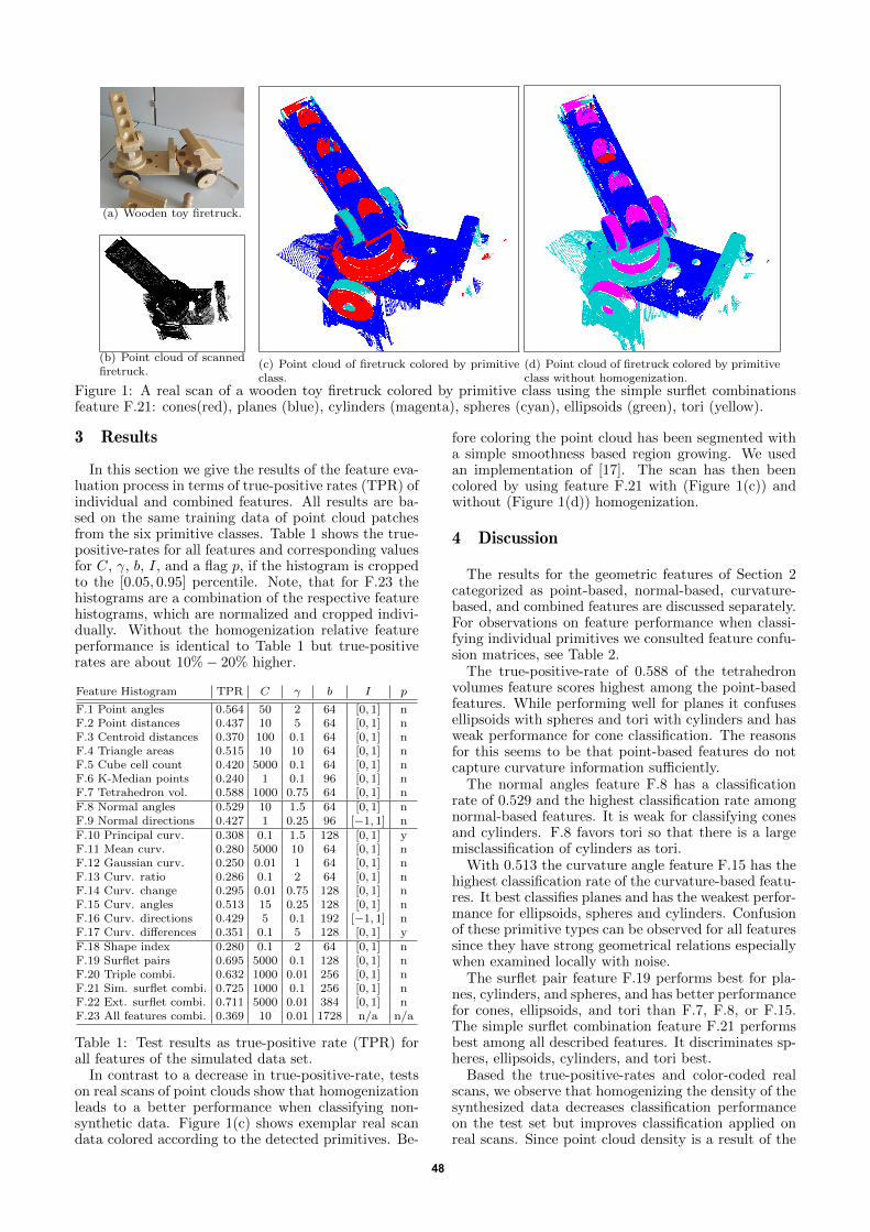
Figure 1: A real scan of a wooden toy firetruck colored by primitive class using the simple surflet combinationsfeature F.21: cones(red), planes (blue), cylinders (magenta), spheres (cyan), ellipsoids (green), tori (yellow).

3 Results

In this section we give the results of the feature eva-luation process in terms of true-positive rates (TPR) ofindividual and combined features. All results are ba-sed on the same training data of point cloud patchesfrom the six primitive classes. Table 1 shows the true-positive-rates for all features and corresponding valuesfor C, γ, b, I, and a flag p, if the histogram is croppedto the [0.05, 0.95] percentile. Note, that for F.23 thehistograms are a combination of the respective featurehistograms, which are normalized and cropped indivi-dually. Without the homogenization relative featureperformance is identical to Table 1 but true-positiverates are about 10%− 20% higher.

Feature Histogram TPR C γ b I p

F.1 Point angles 0.564 50 2 64 [0, 1] nF.2 Point distances 0.437 10 5 64 [0, 1] nF.3 Centroid distances 0.370 100 0.1 64 [0, 1] nF.4 Triangle areas 0.515 10 10 64 [0, 1] nF.5 Cube cell count 0.420 5000 0.1 64 [0, 1] nF.6 K-Median points 0.240 1 0.1 96 [0, 1] nF.7 Tetrahedron vol. 0.588 1000 0.75 64 [0, 1] nF.8 Normal angles 0.529 10 1.5 64 [0, 1] nF.9 Normal directions 0.427 1 0.25 96 [−1, 1] nF.10 Principal curv. 0.308 0.1 1.5 128 [0, 1] yF.11 Mean curv. 0.280 5000 10 64 [0, 1] nF.12 Gaussian curv. 0.250 0.01 1 64 [0, 1] nF.13 Curv. ratio 0.286 0.1 2 64 [0, 1] nF.14 Curv. change 0.295 0.01 0.75 128 [0, 1] nF.15 Curv. angles 0.513 15 0.25 128 [0, 1] nF.16 Curv. directions 0.429 5 0.1 192 [−1, 1] nF.17 Curv. differences 0.351 0.1 5 128 [0, 1] yF.18 Shape index 0.280 0.1 2 64 [0, 1] nF.19 Surflet pairs 0.695 5000 0.1 128 [0, 1] nF.20 Triple combi. 0.632 1000 0.01 256 [0, 1] nF.21 Sim. surflet combi. 0.725 1000 0.1 256 [0, 1] nF.22 Ext. surflet combi. 0.711 5000 0.01 384 [0, 1] nF.23 All features combi. 0.369 10 0.01 1728 n/a n/a

Table 1: Test results as true-positive rate (TPR) forall features of the simulated data set.

In contrast to a decrease in true-positive-rate, testson real scans of point clouds show that homogenizationleads to a better performance when classifying non-synthetic data. Figure 1(c) shows exemplar real scandata colored according to the detected primitives. Be-

fore coloring the point cloud has been segmented witha simple smoothness based region growing. We usedan implementation of [17]. The scan has then beencolored by using feature F.21 with (Figure 1(c)) andwithout (Figure 1(d)) homogenization.

4 Discussion

The results for the geometric features of Section 2categorized as point-based, normal-based, curvature-based, and combined features are discussed separately.For observations on feature performance when classi-fying individual primitives we consulted feature confu-sion matrices, see Table 2.

The true-positive-rate of 0.588 of the tetrahedronvolumes feature scores highest among the point-basedfeatures. While performing well for planes it confusesellipsoids with spheres and tori with cylinders and hasweak performance for cone classification. The reasonsfor this seems to be that point-based features do notcapture curvature information sufficiently.

The normal angles feature F.8 has a classificationrate of 0.529 and the highest classification rate amongnormal-based features. It is weak for classifying conesand cylinders. F.8 favors tori so that there is a largemisclassification of cylinders as tori.

With 0.513 the curvature angle feature F.15 has thehighest classification rate of the curvature-based featu-res. It best classifies planes and has the weakest perfor-mance for ellipsoids, spheres and cylinders. Confusionof these primitive types can be observed for all featuressince they have strong geometrical relations especiallywhen examined locally with noise.

The surflet pair feature F.19 performs best for pla-nes, cylinders, and spheres, and has better performancefor cones, ellipsoids, and tori than F.7, F.8, or F.15.The simple surflet combination feature F.21 performsbest among all described features. It discriminates sp-heres, ellipsoids, cylinders, and tori best.

Based the true-positive-rates and color-coded realscans, we observe that homogenizing the density of thesynthesized data decreases classification performanceon the test set but improves classification applied onreal scans. Since point cloud density is a result of the

48

F.7 Tetrahedron volumes F.8 Normal angles F.15 Curvature angles F.19 Surflet pairs F.21 Simple surflet comb.

Cone

Pla

in

Cyl.

Ellip

s.

Sphere

Tori

Cone

Pla

in

Cyl.

Ellip

s.

Sphere

Tori

Cone

Pla

in

Cyl.

Ellip

s.

Sphere

Tori

Cone

Pla

in

Cyl.

Ellip

s.

Sphere

Tori

Cone

Pla

in

Cyl.

Ellip

s.

Sphere

Tori

Cone 0.19 0.4 0.09 0.15 0.3 0.07 0.3 0.36 0.08 0.17 0.21 0.06 0.32 0.31 0.1 0.16 0.17 0.11 0.58 0.22 0.1 0.06 0.13 0.02 0.67 0.15 0.11 0.06 0.09 0.02

Plain 0.02 1 0 0 0.07 0 0.03 1 0 0.05 0.01 0 0.05 1 0 0.02 0.01 0 0.03 1 0 0 0 0 0.02 1 0 0 0 0

Cyl. 0.02 0 0.47 0.18 0.01 0.47 0.09 0.01 0.35 0.2 0.06 0.42 0.40 0.02 0.41 0.18 0.03 0.45 0.05 0 0.74 0.13 0.01 0.16 0.04 0 0.77 0.09 0 0.17

Ellips. 0.02 0.06 0.09 0.61 0.26 0.11 0.08 0.1 0.09 0.53 0.17 0.17 0.09 0.14 0.16 0.41 0.14 0.2 0.05 0 0.06 0.7 0.16 0.11 0.03 0 0.06 0.74 0.15 0.09

Sphere 0.08 0.17 0 0.12 0.71 0 0.11 0.18 0.03 0.28 0.39 0.07 0.14 0.13 0.08 0.22 0.4 0.08 0.13 0.34 0 0.2 0.65 0 0.12 0.01 0 0.13 0.74 0

Tori 0.02 0 0.22 0.07 0 0.84 0.03 0 0.11 0.01 0.08 0.91 0.04 0.01 0.17 0.06 0.04 0.82 0.01 0 0.2 0.06 0 0.82 0.01 0 0.2 0.07 0 0.8

Table 2: Normalized confusion matrices for features F.7, F.8, F.15, F.19, and F.21 in heat-map coloring.

scanning process it affects features differently for dif-ferent 3d-Scanners. Excluding density as an influenceon feature computation by point cloud homogenizationleads to better generalization of the trained classifier.Using the simple surflet combination feature F.21 weshow an exemplar, colored real scan of a wooden toy fi-retruck, see Figure 1(c). The three main colors are red,blue, and cyan which correspond to cones, planes, andspheres, respectively. There are no tori or ellipsoidswhich is correct for the chosen object. Due to the do-minance of cones in the selected feature, segments thatmight be cylindrical are classified as cones. Withouthomogenizing the density the classifier favors cylindersover cones which in some cases might be correct butoften mistakes planes for spheres or cones, see Figure1(d).

5 Conclusion

We present the evaluation of normal-, point-, andcurvature-based features for primitive recognition inpoint clouds using support vector machines. Based onsimulated scans we compare the performance of dif-ferent features and feature combinations. Resultingclassifiers were applied to real scans with and withouthomogenizing the density. Results of curvature-basedfeatures did not meet our expectations. Our resultscan be used to optimize the feature selection for theclassification task at hand.

For future work we intend to use unsupervised le-arning methods, e.g. auto encoders, for feature engi-neering. To generate simulated scans that match realscans as close as possible is another aspect we plan toinvestigate.

Acknowledgments

This research has been funded by the FederalMinistry of Education and Research (BMBF) ofGermany (project number 02P14A035)

References

[1] T. Rabbani, F. van den Heuvel, and G. Vosselmann,“Segmentation of point clouds using smoothness con-straint,” Int. Archives of Photogrammetry, Remote Sen-sing and Spatial Information Sciences, vol. 36, no. 5,pp. 248–253, 2006.

[2] F. Moosmann, O. Pink, and C. Stiller, “Segmentationof 3d lidar data in non-flat urban environments using alocal convexity criterion,” in Intelligent Vehicles Sym-posium, 2009, pp. 215–220.

[3] Q. Zhana, Y. Liangb, and Y. Xiaoa, “Color-based seg-mentation of point clouds,” Int. Archives of Photo-grammetry, Remote Sensing and Spatial InformationSciences, vol. 38, pp. 248–252, 2009.

[4] R. Schnabel, R. Wahl, and R. Klein, “Efficient RAN-SAC for point-cloud shape detection,” Computer graphicsforum, vol. 26, no. 2, pp. 214–226, 2007.

[5] C. Papazov and D. Burschka, “An efficient RANSACfor 3d object recognition in noisy and occluded sce-nes,” in Computer Vision ACCV 2010, R. Kimmel,R. Klette, and A. Sugimoto, Eds., 2011, pp. 135–148.

[6] K. Denker, D. Hagel, J. Raible, G. Umlauf, and B. Ha-mann, “On-line reconstruction of CAD geometry,” inIntl. Conf. on 3D Vision, 2013, pp. 151–158.

[7] G. Arbeiter, S. Fuchs, R. Bormann, J. Fischer, andA. Verl, “Evaluation of 3d feature descriptors for clas-sification of surface geometries in point clouds,” inInt. Conf. on Intelligent Robots and Systems, 2012,pp. 1644–1650.

[8] R. Rusu, Z. Marton, N. Blodow, and M. Beetz, “Le-arning informative point classes for the acquisition ofobject model maps,” in Int. Conf. on Control, Auto-mation, Robotics and Vision, 2008, pp. 643–650.

[9] R. Osada, T. Funkhouser, B. Chazelle, and D. Dobkin,“Shape distributions,” ACM Trans. on Graphics, vol. 21,no. 4, pp. 807–832, 2002.

[10] F. Cazals and M. Pouget, “Estimating differential quan-tities using polynomial fitting of osculating jets,” Com-puter Aided Geometric Design, vol. 22, no. 2, pp. 121–146, 2005.

[11] J. Koenderink and A. van Doorn, “Surface shape andcurvature scales,” Image Vision Comput., vol. 10, no. 8,pp. 557–565, 1992.

[12] E. Wahl, U. Hillenbrand, and G. Hirzinger, “Surflet-pair-relation histograms: A statistical 3d-shape repre-sentation for rapid classification,” in 3DIM, 2003, pp.474–482.

[13] M. Caputo, K. Denker, M. O. Franz, P. Laube, andG. Umlauf, “Support vector machines for classificationof geometric primitives in point clouds,” in Int. Conf.on Curves and Surfaces, 2014, pp. 80–95.

[14] O. Chapelle, P. Haffner, and V. Vapnik, “Supportvector machines for histogram-based image classifica-tion,” IEEE Trans. on Neural Networks, vol. 10, no. 5,pp. 1055–1064, 1999.

[15] N. Cristianini and J. Shawe-Taylor, An Introductionto Support Vector Machines and other kernel-based le-arning methods. Cambridge University Press, 2000.

[16] B. Schoelkopf and A. Smola, Learning with Kernels.MIT Press, 2001.

[17] R. Rusu and S. Cousins, “3D is here: Point CloudLibrary (PCL),” in Int. Conf. on Robotics and Auto-mation, 2011.

49