Technical Report Documentation Page 1. Report No.

FHWA/TX-06/0-4510-1

2. Government Accession No.

3. Recipient’s Catalog No.

5. Report Date February 2004, Rev. July 2006, 2nd Rev. August 2006

4. Title and Subtitle Evaluation of Equipment, Methods, and Pavement Design Implications of the AASHTO 2002 Axle Load Spectra Traffic Methodology 6. Performing Organization Code

7. Author(s) Feng Hong, Jorge A. Prozzi

8. Performing Organization Report No. 0-4510-1

10. Work Unit No. (TRAIS) 9. Performing Organization Name and Address Center for Transportation Research The University of Texas at Austin 3208 Red River, Suite 200 Austin, TX 78705-2650

11. Contract or Grant No. 0-4510

13. Type of Report and Period Technical (Interim) Report 4510-1 September 2002-August 2003

12. Sponsoring Agency Name and Address Texas Department of Transportation Research and Technology Implementation Office P.O. Box 5080 Austin, TX 78763-5080 14. Sponsoring Agency Code

15. Supplementary Notes Project performed in cooperation with the Texas Department of Transportation and the Federal Highway Administration.

16. Abstract Traffic volume influences the geometric requirements of a highway; however, it is only the axle loads of heavy commercial traffic that affect the structural design of pavements. Mechanistic-based pavement design approaches, coupled with faster computers, are changing the way in which traffic loads are accounted for in pavement design. In the M-E Design Guide for the Design of New and Rehabilitated Pavement Structures, traffic loading will be accounted for by using axle load spectra. Axle load spectra consist of the histograms of axle load distribution for each of four axle types: single, tandem, tridem, and quad. Currently, the Texas Department of Transportation (TxDOT) does not have adequate regional representation of weigh data and uses a statewide average to generate load data for most highways, a practice that is inconsistent with the proposed M-E design approach. This research project will assess and evaluate the implications of the axle load spectra approach proposed by the M-E Design Guide and develop guidelines and recommendations that will facilitate the transition from current practice to the application of the new proposed methodology. The evaluation of current equipment and methodology for traffic data collection and data management will be addressed during the first part of the research project. With these findings in hand, guidelines and recommendations for the implementation of the M-E Design Guide will be developed. Finally, implications for the structural design of pavement will be determined. This interim report presents the findings of the initial literature review, a description of traffic data requirements for the M-E Design Guide for the Design of New and Rehabilitated Pavement Structures, and a preliminary sensitivity analysis conducted under typical Texas environmental conditions. 17. Key Words

Traffic characterization, axle load spectra, traffic classification, WIM, M-E Design Guide, mechanistic design

18. Distribution Statement No restrictions. This document is available to the public through the National Technical Information Service, Springfield, Virginia 22161. www.ntis.gov

19. Security Classif. (of report) Unclassified

20. Security Classif. (of this page) Unclassified

21. No. of pages 94

22. Price

Form DOT F 1700.7 (8-72) Reproduction of completed page authorized

Evaluation of Equipment, Methods, and Pavement Design Implications of the AASHTO 2002 Axle Load Spectra Traffic Methodology Feng Hong Jorge A. Prozzi CTR Technical Report: 0-4510-1 Report Date: February 2004, Rev. August 2006 Research Project: 0-4510 Research Project Title: Evaluate Equipment, Methods, and Pavement Design Implications for Texas

Conditions of the AASHTO 2002 Axle Load Spectra Methodology Sponsoring Agency: Texas Department of Transportation Performing Agency: Center for Transportation Research at The University of Texas at Austin Project performed in cooperation with the Texas Department of Transportation and the Federal Highway Administration.

iv

Center for Transportation Research The University of Texas at Austin 3208 Red River Austin, TX 78705 www.utexas.edu/research/ctr Copyright © 2006 Center for Transportation Research The University of Texas at Austin All rights reserved Printed in the United States of America

v

Disclaimers

Authors’ Disclaimer: The contents of this report reflect the views of the authors, who are responsible for the facts and the accuracy of the data presented herein. The contents do not necessarily reflect the official view or policies of the Federal Highway Administration or the Texas Department of Transportation. This report does not constitute a standard, specification, or regulation.

Patent Disclaimer: There was no invention or discovery conceived or first actually reduced to practice in the course of or under this contract, including any art, method, process, machine manufacture, design or composition of matter, or any new useful improvement thereof, or any variety of plant, which is or may be patentable under the patent laws of the United States of America or any foreign country.

Notice: The United States Government and the State of Texas do not endorse products or manufacturers. If trade or manufacturers’ names appear herein, it is solely because they are considered essential to the object of this report.

Engineering Disclaimer

NOT INTENDED FOR CONSTRUCTION, BIDDING, OR PERMIT PURPOSES.

Project Engineer: Randy Machemehl Professional Engineer License State and Number: 41921

vi

Acknowledgments

The authors want to thank German Claros, PC, Research and Technology Implementation Office; Joseph Leidy, PD, Construction Division; and Richard Rogers, PA, Construction Division for their assistance during the development of this project. Likewise, gratitude is expressed to all the personnel from TxDOT that were involved in the development of field tasks conducted for this project.

Research performed in cooperation with the Texas Department of Transportation.

vii

Table of Contents

1. Introduction................................................................................................................................. 1

1.1 Problem Statement.................................................................................................................1

1.2 Research Goals and Principles...............................................................................................1

1.3 Current Practice of Traffic Data Collection at TxDOT .........................................................3

1.4 Future Development in Truck Weight, Size, and Allowable Axle Loads .............................4

1.5 Research Approach ................................................................................................................5

2. Traffic Characterization .............................................................................................................. 7

2.1 Introduction............................................................................................................................7

2.2 Traffic Load Forecast (ESAL)...............................................................................................7

2.3 Load Spectra ........................................................................................................................13

2.4 Traffic Classifications..........................................................................................................18

2.5 Traffic Load Forecasting .....................................................................................................28

2.6 Economic Effects on Traffic Development—NAFTA........................................................33

3. The M-E Design Guide............................................................................................................. 35

3.1 Background..........................................................................................................................35

3.2 The M-E Design Guide........................................................................................................37

3.3 Mechanistic-Empirical Design Approach............................................................................38

3.4 Traffic inputs in the M-E Design Guide ..............................................................................41

4. Mechanistic Analysis ................................................................................................................ 53

4.1 Sensitivity Analysis .............................................................................................................53

4.2 Results of the Sensitivity Analysis ......................................................................................65

viii

5. Preliminary Conclusions and Future Work............................................................................... 67

5.1 Preliminary Conclusions......................................................................................................67

5.2 Work to be Performed..........................................................................................................69

References..................................................................................................................................... 71

Appendix A................................................................................................................................... 73

ix

List of Figures

Figure 2.1 SDHPT’s Traffic Load Forecasting Procedure........................................................9

Figure 2.2 Tandem Load Spectra Histogram (Expressed in Relative Frequency)..................14

Figure 2.3 Dimensions of Tandem-Axle-Trailer Normally in Operation ...............................14

Figure 2.4 Dimensions of Tridem-axle-trailer Normally in Operation ...................................15

Figure 2.5 General Tandem Axle Load Spectra across All Dates and Locations according to the California Study (Lu and Harvey, 2002).....................................16

Figure 2.6 Tandem Load Spectra in Three Regions of California ..........................................17

Figure 2.7 Typical Truck Profiles for FHWA Classification..................................................21

Figure 2.8 Illustrative Truck Configurations of the U.S. Fleet ...............................................22

Figure 2.9 Typical Truck Profiles for TxDOT Traffic Types .................................................28

Figure 2.10 Impact from Differences in AADT and Truck Growth Rates ...............................31

Figure 2.11 Typical Monthly Volume Patterns (TMG, 2001) ..................................................31

Figure 2.12 Typical Monthly Volume Patterns by WSDOT.....................................................32

Figure 2.13 Projected Volumes for Two-Axle NAFTA Trucks along I-35..............................34

Figure 3.1 Screen for Main Input Variables Required by M-E Design Guide........................42

Figure 3.2 Screen for General Traffic Input Variables ...........................................................43

Figure 3.3 Monthly Adjustment Factors Screen .....................................................................44

Figure 3.4 Vehicle Class Distribution Screen .........................................................................45

Figure 3.5 Hourly Distribution Screen ....................................................................................46

Figure 3.6 Screen Showing Traffic Forecasting Models.........................................................47

Figure 3.7 Axle Load Distribution per Traffic Class and per Axle Type ...............................48

Figure 3.8 Single-Axle Load Distribution...............................................................................48

Figure 3.9 Tandem-Axle Load Distribution............................................................................49

x

Figure 3.10 Tridem-Axle Load Distribution .............................................................................49

Figure 3.11 Screen Showing Expected Number of Axles per Truck ........................................50

Figure 3.12 Mean Axle Configuration Parameters ...................................................................51

Figure 3.13 Mean Wheelbase Dimensions for Short, Medium, and Long Units .....................52

Figure 3.14 Flow Chart of Traffic Input to Obtain Axle Load Spectra.....................................52

xi

List of Tables

Table 2.1 Example of a Weight Distribution Table for RDTEST68 .......................................9

Table 2.2 ESAL Input Coefficient of Variance .....................................................................12

Table 2.3 Input Contributions to Variance of Typical Forecast ............................................12

Table 2.4 Axle Load Spectra (Expressed in Absolute Frequency) ........................................13

Table 2.5 ASTM Vehicle Classes (Standard Specification E1318-94, 1996) .......................19

Table 2.6 Length-Based Classification Boundaries...............................................................23

Table 2.7 WIM Vehicle Classifications by Caltrans..............................................................24

Table 2.8 Typical Vehicle Profiles for Caltrans Truck Types ...............................................25

Table 2.9 TxDOT Vehicle Classification Table (by Axle Spacing) ......................................27

Table 2.10 Functional Classes of Roadways ...........................................................................32

Table 2.11 U.S.-Mexico Truck Axle Weight Limits ...............................................................34

Table 3.1 Hierarchical Approach for Three Design Levels ...................................................41

Table 3.2 Monthly Adjustment Factors (WIM D512, 2000) .................................................44

Table 3.3 Vehicle Class Distribution in (WIM D512, 2000).................................................45

Table 3.4 Average Hourly Traffic Distribution (WIM D512, 2000) .....................................46

Table 3.5 Traffic Growth Factors ..........................................................................................47

Table 3.6 Number of Axles per Truck ...................................................................................50

Table 4.1 Pavement Structures Used in the Preliminary Analysis ........................................54

Table 4.2 Load and Axle Configurations...............................................................................56

Table 4.3 Traffic Volumes Expressed in Terms of AADTT Values .....................................56

Table 4.4 Amarillo Heavy Pavement Load Data ...................................................................58

Table 4.5 Austin Heavy Pavement Load Data.......................................................................59

Table 4.6 El Paso Heavy Pavement Load Data .....................................................................59

xii

Table 4.7 Houston Heavy Pavement Load Data ....................................................................60

Table 4.8 Amarillo Light Pavement Load Data.....................................................................60

Table 4.9 Austin Light Pavement Load Data.........................................................................61

Table 4.10 El Paso Light Pavement Load Data .......................................................................61

Table 4.11 Houston Light Pavement Load Data......................................................................62

Table 4.12 Amarillo Heavy Pavement AADTT Data..............................................................63

Table 4.13 Austin Heavy Pavement AADTT Data..................................................................63

Table 4.14 El Paso Heavy Pavement AADTT Data ................................................................63

Table 4.15 Houston Heavy Pavement AADTT Data...............................................................63

Table 4.16 Amarillo Light Pavement AADTT Data................................................................64

Table 4.17 Austin Light Pavement AADTT Data ...................................................................64

Table 4.18 El Paso Light Pavement AADTT Data..................................................................64

Table 4.19 Houston Light Pavement AADTT Data ................................................................64

Table 4.20 Summary of Exponents of the Power Law ............................................................65

1

1. Introduction

1.1 Problem Statement Total volume of traffic affects the geometric requirements of highways; however, it is

only the axle loads of heavy commercial traffic that affect the structural design of pavements. 85 the proximity of the project and accounting for potential changes in land use and

development and the fact that the construction of a new highway tends to divert traffic from other routes in the proximity. In addition, the historical trend of increasing legal loads, the recent decline of railroad services, and the fast economic growth of the nation have all contributed to the underestimation of traffic growth. After the North American Free Trade Agreement (NAFTA) became effective in 1994, the surge of commercial vehicles on Texas highways made it even more difficult to predict traffic loads. For these reasons, estimates of cumulative design traffic for many pavement structures frequently have been grossly miscalculated.

Mechanistic design principles, coupled with the increasing availability of more powerful and faster desktop computers, are rapidly changing the way in which traffic loads are accounted for in pavement design. In the Mechanistic-Empirical Guide for the Design of New and Rehabilitated Pavement Structures, hereafter referred to as the M-E Design Guide (www.2002designguide.com), traffic is accounted for by using axle load spectra. For the most accurate design cases, weigh-in-motion (WIM) data from the highway to be rehabilitated will be used with appropriate growth factors, projected to the length of the analysis period. Highways to be constructed on new right-of-ways will require traffic data estimates from highways in close proximity. For intermediate design levels, regional axle load spectra data from facilities with similar truck volumes, and site-specific traffic classifications and counts will be used. Finally, for the less accurate design levels, actual traffic counts or estimates will be used in conjunction with statewide classifications and WIM information.

Currently, there are approximately twenty WIM stations in Texas; the majority of them are on high-volume facilities such as interstate, state and U.S. highways. Increased WIM density and sampling frequency are necessary to ensure adequate traffic forecasting, especially on lower-volume facilities. Currently, the Texas Department of Transportation (TxDOT) does not have adequate regional representation of weigh data and uses a statewide average to generate load data for most highways (Middleton and Crawford, 2001). The need for improved WIM calibration standards has also been identified; however, the level of acceptable precision is unknown. Setting a fixed level of WIM precision is complicated by the uncertainties of forecasting traffic for 20, 40, or more years into the future. Similarly, the density of vehicle classification and count devices to support designs using regional WIM data are not clearly defined.

1.2 Research Goals and Principles The goal of this research project is to assess and address the implications of the axle load

spectra approach proposed by the M-E Design Guide. These implications have several dimensions. On the one hand, the evaluation of current equipment and methodology for data collection and data management should be addressed. On the other hand, the implications on the structural design of pavement should be evaluated.

2

Other objectives include the identification of issues related to data collection, data reduction, and end-use aspects; determination of spatial and temporal distribution of data collection, and the accuracy and calibration of collecting devices; development of guidelines for the transferability of data from the Traffic Analysis Section to the department’s pavement designers; and the development of guidelines and recommendations for the application of the various levels of design proposed in the M-E Design Guide.

Pavement structures deteriorate under the combined action of traffic loading and the environment; hence, both aspects should be considered in the design of new and rehabilitated pavements. Because of the large annual investment in the state highway system, any effort to optimize the use of highway funds will have a significant impact in the economy of the state. The development of the M-E Guide is one such effort. The current American Association of State Highways and Transportation Officials (AASHTO) Design Guide (AASHTO, 1993) is empirically based. The design equations are mainly based on the analysis of the results of the AASHTO Road Test carried out in the late 1950s and early 1960s (HRB, 1962).

The empirical nature of the current AASHTO guide introduces a degree of uncertainty that cannot be estimated when the design procedure is applied outside its original data range. Some of the most important limitations of the current approach include the following:

Traffic. The original design equations were developed based on the deterioration from approximately one million axle load repetitions. Current interstate designs should accommodate 50 to 200 million axle loads during their design life. The uncertainty introduced by such extrapolation cannot be evaluated. In addition, the configurations of heavy commercial vehicles have changed dramatically since the AASHTO Road Test and they continue to change.

Environmental conditions. The AASHTO Road Test was conducted near Ottawa, Illinois; therefore, the environmental conditions are not particularly applicable to Texas.

Materials. Only one set of asphalt mixture, base, subbase, and subgrade materials were used in the main experimental design. Pavement design using other materials introduces unknown uncertainties. Although later versions of the AASHTO Guide have been improved to include new results and the application of basic mechanistic principles, the empirical nature still remains intrinsic.

Distress mode. The riding quality in terms of the present serviceability index was the adopted distress mode. A comprehensive design methodology should consider a number of indicators, such as fatigue, thermal and reflection cracking, rutting of asphaltic and unbound granular materials, and roughness progression.

Rehabilitation. Although a number of test sections were overlaid and evaluated during the AASHTO Road Test, these results were not incorporated in the development of the main design equations. Later guides have included rehabilitation considerations by means of applying nondestructive testing and mechanistic concepts. The new M-E Design Guide attempts to overcome the above limitations by incorporating

a mechanistic-based approach. Pavement design will be addressed following a holistic approach including the assessment of the environmental conditions, material properties, traffic characterization, construction-related issues, and quality control and assurance (ERES, 2001a). Of course, these improvements will come at a cost: while the mechanistic approach to pavement

3

design is more rational than its empirical counterpart, it is also technically more demanding and data intensive. These are some of the areas that will require increased involvement: characterization of the subgrade or existing pavement (in case of rehabilitation); characterization of the structural material properties; evaluation and assessment of local environmental effects; and a more detailed characterization of the design traffic loading.

The hierarchical design approach of the M-E Guide provides flexibility to obtain design inputs based on the importance of the project and the availability of resources. This approach is applied to traffic, materials, and environmental inputs.

1.3 Current Practice of Traffic Data Collection at TxDOT

1.3.1 RDTEST68 TxDOT currently has approximately twenty WIM sites in operation, mainly located on

interstate facilities. The Federal Highway Administration (FHWA) Traffic Monitoring Guide (FWHA, 2001) recommends the use of at least ninety sites for monitoring state traffic. Very detailed information is available regarding vehicle classification and weights. Most data required to use the proposed M-E Guide are available; however, guidelines on temporal and spatial distribution and data management are required.

At the request of the districts, traffic data, in terms of numbers of equivalent single-axle loads (ESALs), are made available to the pavement designer. Traffic data include roadway and vehicle characteristics as well as estimates of the number of ESALs expected on a particular facility. The RDTEST68 program calculates the ESALs for the specified period. This calculation is based on assumptions for average daily traffic (ADT), growth rate, percentage of trucks, percentage of single axles, axle factors, axle weight distribution, directional and lane distributions, and design period. Each of these variables has an inherent variability that is incorporated into the ESAL estimation, producing estimates of low reliability. Furthermore, when specific data are not available for a site, this estimation is based on a statewide average axle distribution. A gap, therefore, exists between the state-of-practice at TxDOT and the requirements of the M-E Design Guide. Some of the most critical issues for closing this gap are the spatial (WIM distribution) and temporal (frequency) coverage and the level of accuracy.

Spatial coverage is probably the most difficult issue to address immediately because of its cost implications. There is currently a gap of seventy-five WIM stations between the number of stations recommended by FHWA and the current coverage. In terms of temporal coverage, the issue is the number of personnel required to operate these facilities at the frequency required. This, in turn, is related to the level of detail that will be required by the M-E Design Guide. Most of the specific information is currently being collected. The determination of level of accuracy requires more extensive research. The selection of the level of accuracy will depend on the intended use of the traffic data. Due to the multiple uses of traffic data, a multidimensional approach should be followed to determine the optimum accuracy. It is expected that the accuracy requirements should not be constraining for pavement design because of the multiple uncertainties inherent to the structural design of pavements.

1.3.2 The STARS Program The Strategic Traffic Analysis and Reporting System (STARS) is a project sponsored by

the Transportation Planning and Programming (TPP) Division of TxDOT. STARS is under

4

development in partnership with FHWA and the Texas Department of Transportation Information Systems Division (ISD). The system is intended to serve as the next-generation system for analyzing and reporting traffic data on the basis of easy information access and user friendliness. STARS is designed to be a web-based system utilizing state-of-the-art information technologies such as multi-tiered client/server, relational database management systems (DBMS), and the geographic information systems (GIS). STARS is designed to comply with new federal mandates for traffic collection, monitoring, analysis, and reporting. These mandates include:

2001 FHWA Traffic Monitoring Guide

M-E Pavement Design Guide

TEA 21 for Forecasting, Modeling, and Planning

“Truth in Data”—Substantiating by Comparing Quantitative with Historic Data This compliance suggests that the provision of traffic data required by the M-E Guide

should be integral to the design of the STARS system. But as STARS is still under development, it is not clear to what extent it will fully support the M-E Guide. It is then critical that the capabilities of the STARS program be reviewed with regard to its potential support to the M-E Guide. The impact of the STARS system on the implementation by TxDOT of the new guide should not be neglected.

The life cycle for any data item, including traffic data, is composed of data collection, management, and usage. A good coordination of the steps involved in the process is the key to the success of the overall process. In the case of traffic information, the data collection and analysis is done by the Transportation Planning and Programming (TPP) Division, Traffic Analysis Section. This section will continue to process and manage data procured through the STARS system. According to the current framework, STARS should provide the data to the pavement designer as part of the data usage. Therefore, good coordination of the involved parties and components is critical for the successful implementation of the new M-E Design Guide.

1.4 Future Development in Truck Weight, Size, and Allowable Axle Loads Most pavement structural damage is caused by heavy commercial vehicles. For example,

according to FHWA, 21 percent of the total state highway capital expenditures was used for pavement resurfacing, restoration, and rehabilitation (RRR) in 1998 (FHWA, 1999). In its 1997 highway cost allocation study, the U.S. Department of Transportation allocated 77 percent of RRR costs to medium and heavy trucks (DOT, 1997). In other words, the weight, size, axle configuration, and related characteristic of trucks have an important impact on the pavement deterioration process.

Since pavement structures are normally designed for a period of 20 to 40 years or more and the characteristics of heavy commercial vehicles are constantly changing, future trends in truck weight, size, axle configuration, and related characteristics must be taken into consideration when estimating design traffic, especially traffic growth rates. Some of the current and expected trends are the following:

Tire Pressure. Tires used in the AASHTO Road Test were bias-ply tires with inflation pressures between 75 and 80 psi. Since then, bias-ply tires have been replaced by radial tires and inflation pressures have increased. According to a survey conducted in

5

seven states from 1984 to 1986, 75 to 80 percent of the trucks used radials tires with an average tire pressure of 100 psi (Bartholomew, 1989). A most recent study in Texas determined an average tire pressure of 96.8 psi with a standard deviation of 15 psi on a state-wide sample of 9,600 tires (Wang et all, 2000). Higher tire pressures result in higher contact stresses between the tire and pavement. The increased contact stresses increase the potential for permanent deformation of the asphalt layers and the occurrence of top-down fatigue cracking.

Single and Dual Tires. The AASHTO load equivalency factors strictly apply to dual-wheeled axles. Recent increases in steering-axle loading and more extensive use of single tires on load-bearing axles have prompted efforts to examine the effect of single tires on pavement deterioration. Different studies have indicated that, everything else being equal, single tires are more damaging to pavement structures than dual tires (Prozzi and de Beer, 1997).

Suspension System. The dynamic axle load of a heavy commercial vehicle fluctuates above and below its static load. The degree of fluctuation depends on factors such as pavement roughness, vehicle speed, radial stiffness of the tires, mechanical properties of the suspension system, and the overall configuration of the vehicle. Assuming that the damage effects of dynamic axle loads are similar to those of static axle loads, increases in vehicle dynamics accelerate pavement damage. A study conducted by the Organization for Economic Cooperation and Development (OECD, 1982) found that the reduction in dynamic effects due to improved suspension systems might reduce pavement damage effects by about 5 percent.

Axle Spacing. As the spacing between two axles is reduced, the stress distribution induced in the pavement structure by each axle begins to overlap. The maximum deflection of the pavement continues to increase as axle spacing is reduced. The vertical strain in the unbound materials also increases, while the maximum horizontal tensile strains in the bound layers may increase or decrease depending on the structure. As a result, very distinct damage is produced to the pavement structure (Prozzi and de Beer, 1997).

1.5 Research Approach The key to the successful implementation of the M-E Pavement Design Guide is

dependent not only on the adequate provision of the required traffic data, but also on the clear understanding of the implications of the new design method on the design results. The research requires extensive knowledge not only of pavements and traffic, but also, more importantly, of the interactions between traffic and pavements. Knowledge of future trends in truck weight, size, and axle configuration as well as of the impact of these trends on pavement design is also critical to the successful implementation of the new design method. Development of recommendations for collecting and analyzing traffic data in support of the implementation of the M-E Guide at TxDOT must

consider the current engineering practice and business environment at TxDOT so that the use of existing resources can be maximized and the disruption to current practices can be minimized;

6

clearly identify and adequately address the implications of the recommended traffic data collection and analysis procedures and issues critical to the implementation of the recommended procedures; and

ensure that the implications of the new design method on the design results are fully understood. Successful completion of this research project will provide TxDOT with a reliable

methodology to assess all traffic-related issues necessary for the implementation of the forthcoming M-E Guide. The procedures and recommendations developed during this research program will be used in district and area offices statewide.

The benefits of this project will include a reliable method for accounting for traffic loading in the pavement design process at the various levels of accuracy as well as detailed recommendations for traffic data management and guidelines for the selection of the specific design level. The significant consequence will be improved resource utilization with associated cost savings for a more reliable pavement design procedure at TxDOT.

7

2. Traffic Characterization

2.1 Introduction Structure and material properties, traffic characterization, and environmental conditions

are the three major input variables for pavement design and rehabilitation. The life of a pavement structure is the result of the interaction between these variables. Environmental factors mainly refer to temperature and precipitation regimes, drainage, and location of the water table. Traffic should include the axle and wheel configuration, load and stress magnitude, and the number of repetitions applied to the pavement. As one of the major factors for pavement design and rehabilitation, it is of great importance to accurately forecast the traffic loading expected to be applied to the pavement during its service life. Moreover, obtaining the most precise truck loading prediction information is a critical issue, because it is the truck load that accounts for the dominant structural damage to pavement. For this reason, the focus of this section is on the forecast of truck load based on truck classes and load spectra.

2.2 Traffic Load Forecast (ESAL) In the current AASHTO Design Guide (AASHTO, 1993), accumulated equivalent single

axle loads (ESALs) are utilized to measure the anticipated traffic load that is applied to pavement over its design life. Pavement design methods based on ESALs are widely used in all the states in the U.S and overseas. With the development of new mechanistic-empirical design methods, current design methods have been upgraded and are becoming more reliable in terms of the traffic load characterization. Various states have conducted research for the implementation of more precise traffic load forecasts while applying the AASHTO pavement design concept to their local conditions. For instance, TxDOT uses the RDTEST68, which was developed by the Traffic Analysis Branch of the Transportation Planning and Programming Division to predict future traffic for pavement design based on a road test conducted on Texas highways in 1968. RDTEST68 is a computer program specifically developed for traffic forecasting purposes. The Minnesota Department of Transportation (MnDOT) has developed its own program, MNESALS, which was developed by the Office of Transportation Data and Analysis to forecast design traffic. However, it is expected that until the final implementation of the upgraded M-E Pavement Design Guide, design traffic loading will still be accounted for in terms of ESALs. Two major differences are expected in the forthcoming M-E pavement design procedures regarding traffic inputs:

(i) load forecasts will be based on classified traffic, which has already been applied in some states, and (ii) load spectra per class and per axle type will be used.

2.2.1 Traffic Forecasting Procedures in Texas TxDOT uses a computer program, RDTEST68, to calculate the total ESAL and the

design lane ESAL forecasts for pavement design. In TxDOT Research Project 0-1235 (Vlatas and Dresser, 1991), the Texas Transportation Institute (TTI) identified four key assumptions for the TxDOT traffic forecasting model, one “linear” and three “constant”:

8

Annual traffic growth follows a linear model;

Percentage of trucks remains constant over the design period;

The truck traffic stream makeup remains constant over the design period; and

The average load equivalency factor per truck remains constant over the design period. However, recent research on truck traffic in Texas shows that these assumptions are not

appropriate for an accurate traffic load forecast. For example, concerning the input component of percentage of trucks, the research conducted by Bass and Dresser (1994), also at TTI, found that as a planning parameter, percentage of trucks can range between 2 and 10 percent with a variation from the mean of plus/minus 67 percent. This percentage can be significantly higher over short periods of time.

The RDTEST68 program flow chart is depicted in Figure 2.1 (Cervenka and Walton, 1984). The following paragraphs explain the major steps, which were designed by the Texas State Department of Highways and Public Transportation (SDHPT, former name of TxDOT).

(1) Preparation of weight data. Several additional computer programs are used to convert raw weight data into a format

usable by the RDTEST68 program, among which WIM82 is a key program that performs the “data reduction.” The basic steps of the WIM82 computer program are as follows:

For each vehicle type and weight group, the weight data collected over the most recent three-year period are tabulated for all single axles and all tandem axles.

Based on vehicle classification and count data, the number of single and tandem axles for each vehicle group is calculated.

The axle weight data are prorated by the count data, with all single axles combined by weight group and all tandem axles combined by weight group.

The number of axles in each weight group is shown as a percentage of the total. As a result, the final table of the percentage of each load bin of single and tandem axle

groups for each WIM station is obtained as the basic weight table, as shown in Table 2.1 with sample data from Station 501, 1981 to 1983 (Cervenka and Walton, 1984).

9

Figure 2.1 SDHPT’s Traffic Load Forecasting Procedure

(2) Selection of a representative station The procedure is to select one weight table from a “representative” WIM station (three

years’ data) and assume that its axle weight distribution is similar to that of the highway segment of interest, largely based on engineering judgment. If a representative station does not exist for a particular project then the statewide average is used.

Table 2.1 Example of a Weight Distribution Table for RDTEST68 Single Axles Tandem Axles Upper Weight

Limit (lbs.) Percent Cumulative Percent Cumulative 2,000 3,000 4,000 5,000 6,000 7,000 8,000 9,000 10,000 11,000 12,000 13,000 14,000

0.213 0.419 1.625 2.344 2.729 3.268 4.978 7.46 9.291 7.161 3.413 1.89 1.069

0.213 0.632 2.257 4.601 7.330 10.598 15.576 23.036 32.327 39.488 42.901 44.791 45.860

0.000 0.017 0.000 0.000 0.068 0.119 0.231 0.727 1.411 2.369 2.669 2.190 2.318

0.000 0.017 0.017 0.017 0.085 0.204 0.435 1.162 2.573 4.942 7.611 9.801 12.119

Inputs: i. ADT

ii. Growth Rate iii. Design Period iv. Percentage of Trucks v. Percent Single Axles

vi. Axle Factors vii. Structural Number

(flexible pavement) viii. Slab Thickness (rigid

pavements)

Single axle/tandem axle load distribution for each station

WIM data ADT by classes and by station

WIM82

User selection of a representative weight

Single axle/tandem axle load distribution for each station

RDTEST68

10

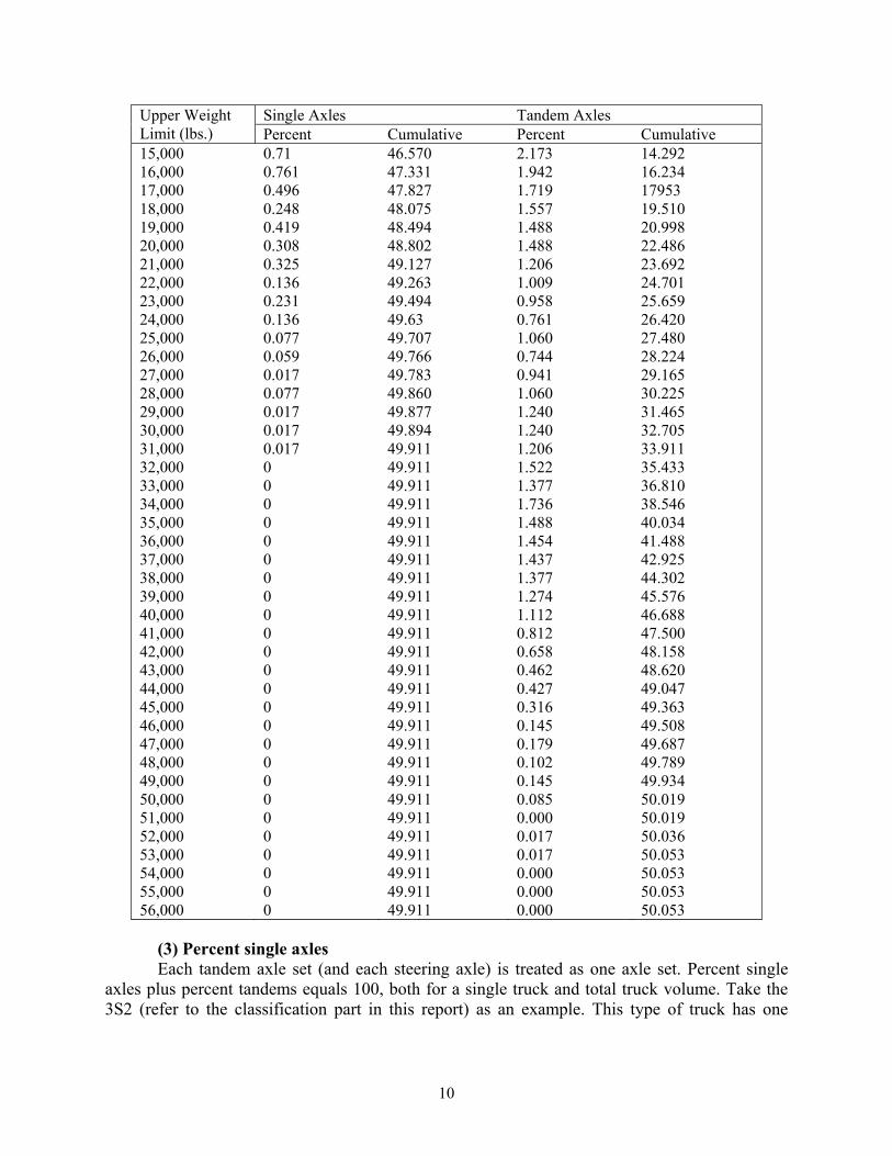
Single Axles Tandem Axles Upper Weight Limit (lbs.) Percent Cumulative Percent Cumulative 15,000 16,000 17,000 18,000 19,000 20,000 21,000 22,000 23,000 24,000 25,000 26,000 27,000 28,000 29,000 30,000 31,000 32,000 33,000 34,000 35,000 36,000 37,000 38,000 39,000 40,000 41,000 42,000 43,000 44,000 45,000 46,000 47,000 48,000 49,000 50,000 51,000 52,000 53,000 54,000 55,000 56,000

0.71 0.761 0.496 0.248 0.419 0.308 0.325 0.136 0.231 0.136 0.077 0.059 0.017 0.077 0.017 0.017 0.017 0 0 0 0 0 0 0 0 0 0 0 0 0 0 0 0 0 0 0 0 0 0 0 0 0

46.570 47.331 47.827 48.075 48.494 48.802 49.127 49.263 49.494 49.63 49.707 49.766 49.783 49.860 49.877 49.894 49.911 49.911 49.911 49.911 49.911 49.911 49.911 49.911 49.911 49.911 49.911 49.911 49.911 49.911 49.911 49.911 49.911 49.911 49.911 49.911 49.911 49.911 49.911 49.911 49.911 49.911

2.173 1.942 1.719 1.557 1.488 1.488 1.206 1.009 0.958 0.761 1.060 0.744 0.941 1.060 1.240 1.240 1.206 1.522 1.377 1.736 1.488 1.454 1.437 1.377 1.274 1.112 0.812 0.658 0.462 0.427 0.316 0.145 0.179 0.102 0.145 0.085 0.000 0.017 0.017 0.000 0.000 0.000

14.292 16.234 17953 19.510 20.998 22.486 23.692 24.701 25.659 26.420 27.480 28.224 29.165 30.225 31.465 32.705 33.911 35.433 36.810 38.546 40.034 41.488 42.925 44.302 45.576 46.688 47.500 48.158 48.620 49.047 49.363 49.508 49.687 49.789 49.934 50.019 50.019 50.036 50.053 50.053 50.053 50.053

(3) Percent single axles Each tandem axle set (and each steering axle) is treated as one axle set. Percent single

axles plus percent tandems equals 100, both for a single truck and total truck volume. Take the 3S2 (refer to the classification part in this report) as an example. This type of truck has one

11

single axle and two tandems. Hence, it has a “percent single axles” factor of (100 percent) × (1/3) = 33.33 percent.

(4) 18-KESALs per truck axle By default, RDTEST68 program estimates equivalency factors for flexible pavements

with a structural number of 3 and a concrete slab thickness of 8-in. For all other thicknesses, the factors are calculated from the AASHTO equations embedded in the RDTEST68.

(5) Axle factor The axle factor is the average number of axles on a truck. In order to calculate the axle

factor, available vehicle classification data at (or near) the highway segment under study is normally utilized. For example, a 2S3 truck (1 steering axle, 1 single axle with dual wheels, and 1 tridem axle) would have an axle factor of 3.00, which is the same as the axle factor of a 3S2 truck (1 steering axle and 2 tandem axles).

(6) Traffic forecast The total traffic expected to utilize the pavement facility during the design period in

terms of ESALs is calculated by the following steps:

]2/)2[(_ 0 TTGFADTvehiclesTotal ADT ××+×= (2.1) PCTvehiclesTotaltrucksTotal ×= __

trucksTotalvehiclesTotalvehiclesOther ___ −= 000626.0_)/18(_18_ ×+−×=− vehiclesOthertruckKESALstrucksTotalKESALsTotal

Where: ADT0 : initial ADT, i.e., base year ADT (vpd) GFADT : ADT growth factor (percent volume growth per year) T : design period PCT : percentage of trucks Theoretically, the total ESALs should include the contribution from other vehicles

besides trucks. Therefore, when other vehicles are considered (primarily automobiles), the factor 0.000626 ESAL per vehicle can be utilized to compute their contribution to the impact on the pavement. Given the low contribution to total ESALs by “other vehicles,” this part of the total ESAL calculation equation is usually omitted.

According to the work on ESAL forecasting by Vlatas and Dresser (1991) at TTI, it was found that the ADT growth factor possessed the largest coefficient of variance among all the input components, while the percentage of trucks and directional distribution contributed most to the variance of the forecast result. Table 2.2 and 2.3 show the detailed values for each component in question.

12

Table 2.2 ESAL Input Coefficient of Variance Component Coefficient of variance (%) Base Year ADT 2.1 – 10.9 ADT Growth Factor 29.3 Percentage of Trucks 13.4 – 47.5 Percentage of Single Axles ≤ 19.7 Truck Axle Factor ≤ 10.8 Average Load Equivalency Factor per Truck 0 – 23.1 Directional Distribution 34.4 Lane Distribution Factor 7.7

Table 2.3 Input Contributions to Variance of Typical Forecast Component Contribution to Variance (%) Percentage of Trucks 38 Directional Distribution 38 Average Load Equivalency Factor per Truck 17 Base Year ADT <4 Lane Distribution Factor <2

2.2.2 MNESAL Program for Traffic Load Forecast The Minnesota Department of Transportation (MnDOT) is using the computer program

MNESAL to forecast traffic loading in terms of ESALs for pavement design (Nelson, 2002). Three pieces of equipment are utilized to collect raw data: weight in motion (WIM), automatic traffic recorder (ATR), and pneumatic tubes (PT). The WIM data are mainly from the Minnesota Road Research Project (MnRoad) and 26 statewide stations. ATR provides the data from 160 statewide sites and 22 speed sites. For collecting the AADT information, one tube is used, while two tubes are applied for the purpose of vehicle classification information. The inputs of MNESAL include past traffic volumes (twenty years), past vehicle classification distributions (twenty years), axle load equivalent factors, and design lane factor. The outputs consist of projected AADT, projected HCAADT (Heavy Commercial Annual Average Daily Traffic), 20- and 35-year design lane ESALs, and documentation of work performed.

Vehicle classification data is available in the program of MNESALS, where an eight-category scheme was adopted by MnDOT to calculate average vehicle percentages, average truck volumes, and ESALs. The eight categories of vehicles are cars, 2 ASU (two axles, six tires, single unit), 3 + ASU (three axles, single unit), 3ASemi (three axles, semi trailer), 4ASemi (four axles, semi trailer), TT/BUS (two or three axles, bus), Twins (twin trailers), and 5 + ASemi (five axles, semi trailer). All categories excluding cars are referred to as heavy commercial traffic (HCT), i.e., trucks and buses. Additionally, due to the dominant percentage in the total traffic count and its particular effect on pavement performance, the typical 5 + ASemi category is further split in two: common 5 Ax Semi and heavy 5 Ax Semi. The heavy 5 Ax Semi is defined as tank, dump, grain, and stake if on a timber route Dist 1, 2, or 3, where the tank, dump, and grains and sometimes stakes constitute 30 percent or more of the five-axle semis.

13

Theoretically, traffic load (ESAL) forecasts are the combination of two components created by contributions from cars as well as from heavy commercial traffic. When performing an ESAL forecast, cars are not counted due mainly to their negligible impact on the pavement performance. The consideration of axle loading involves single axle, tandem, tridem, and more axle groups. A least squares model is used by MNESALS to forecast the AADT for mixed traffic as well as for cars and heavy commercial traffic. It is usually assumed that the growth rates for all types of trucks are the same, i.e., the percentage of each type of vehicle remains the same in the forecast year as in the base year. In fact, there could be inconsistent rates of growth among the traffic classes.

2.3 Load Spectra The concept of load spectra, as a critical input for pavement design, has gained wide

acceptance in recent years. The Portland Cement Association (PCA) method of pavement design has incorporated detailed load spectra information since 1966. In the M-E Design Guide for the Design of New and Rehabilitation Pavement structures, traffic loading will be accounted for by using axle load spectra. A load spectrum can be defined as the load distribution of an axle group during a period of time. The axle load spectra consist of the histograms of axle load distribution for each of four axle types: single, tandem, tridem, and quad. An example of axle load spectrum given by the M-E Design Guide is shown in Table 2.4. The corresponding histogram of the data of tandem axle load distribution in Table 2.4 is presented in Figure 2.2.

According to the Federal Highway Administration (FHWA), among the four types of axle groups, a single axle is defined as an axle on a vehicle that is separated from any leading or trailing axle by more than 96 inches, and includes both the single axle with single tires or dual tires. A tandem axle refers to two consecutive axles that are more than 40 inches but not more than 96 inches apart and are articulated from a common suspension system. In the same way, for a group of three axles, if both of the distances between the consecutive axles are more than 40 inches but not more than 96 inches, it is a tridem. In some states, spread tandem is further defined as a special case of two axles that are articulated from a common attachment but are considered to be two single axles rather than one tandem, because they are separated by more than 96 inches. As examples, Figure 2.3 and Figure 2.4 give an illustration of normally operating tandem and tridem axle spacing configurations (Gindy and Kenis, 1998).

Table 2.4 Axle Load Spectra (Expressed in Absolute Frequency) Number of Axles Axle Load (1000lb)

Single Tandem Tridem Quad >11 - 15 >15 - 19 >19 - 23 >23 - 27 >27 - 31

5,000 3,000 200 50 6

400 2,000 5,000 4,000 2,000

100 500 800 1,000 1,500

5 10 30 80 100

14

Figure 2.2 Tandem Load Spectra Histogram (Expressed in Relative Frequency)

Figure 2.3 Dimensions of Tandem-Axle-Trailer Normally in Operation

15

Figure 2.4 Dimensions of Tridem-axle-trailer Normally in Operation

With the imminent advent of load spectra as an input for pavement design, various states in the U.S., including California, Kentucky, Minnesota, Washington, and Texas, have launched pavement research projects with a load spectra orientation.

Based on the WIM data collected from 1991 to early 2001 on the California state highway network (approximately 101 WIM stations), the Pavement Research Center at the University of California, Berkeley, has carried out research on the characteristics of axle load spectra (Lu and Harvey, 2002). One of the center’s major objectives in the study concerning load spectra was to develop axle load spectra for various axle groups of each truck type and to compare these load spectra among various locations and time periods. The axle groups involved steering axle, single axle, tandem, and tridem. Vehicles were classified into fifteen categories. Three locations were covered: the Bay Area, Central Valley, and Southern California. Time periods investigated include hour of the day, day of the week, and seasonal variation. An example of general tandem load spectra developed in California is illustrated in Figure 2.5.

16

Figure 2.5 General Tandem Axle Load Spectra across All Dates and Locations

according to the California Study (Lu and Harvey, 2002)

The load spectra presented in Figure 2.5 can provide detailed information on the tandem axle load. Among all the trucks, it is obvious that truck type 9 (five-axle truck or “eighteen-wheeler”) accounts for the dominant percentage such that the total truck pattern is determined by this type of truck. The two peaks are also characteristic of the major heavy commercial vehicles, representing the empty cargo and full cargo situations. By comparing load distribution and legal limit weight for tandem in the spectra chart, it is easy to find the percentage of those axles that are overweight.

Another example is given in Figure 2.6 to show the relationship among the different locations in California in terms of tandem axle weight distribution. The load spectra from the three locations exhibit a similar pattern, each with two peaks at almost the same axle weight points. However, we can find by comparison that the load is heavier in the Central Valley than the other two locations, because its heavier load peak accounts for more frequency.

17

Figure 2.6 Tandem Load Spectra in Three Regions of California

The main findings of the California study can be summarized as follows:

Nearly all steering axle loads were less than 90 kN (20.2 kips); nearly all single axle loads were less than 110 kN (24.7 kips); nearly all tandem axle loads were less than 210 kN (47.2 kips); nearly all tridem axle loads were less than 260 kN (58.5 kips); and all four axle types had a bimodal pattern of load spectra.

Axle loads were heavier at night than during the daytime. The proportion of larger truck types, such as Class 9, more typically used as a long-haul truck, increased at night, while the proportion of smaller truck types, such as Class 5, typically used for shorter deliveries, decreased at night.

Study of geographical differences showed that load spectra were much higher in Central Valley than in the Bay Area and Southern California, particularly for tandem axles. Axle load spectra were much higher at rural WIM stations than at urban WIM stations.

Steering axle load spectra were similar across all six stations, while load spectra for other axle types varied considerably across the six stations. Axle load spectra for steering and single axles remained fairly constant across the years, and tandem and tridem axles exhibited yearly variation with no particular trend.

Axle spectra were similar for both directions and much heavier in the outside lanes. For facilities with two lanes in each direction, more than 90 percent of the truck traffic traveled in the outside lane. For facilities with three or more lanes in each direction, more than 90 percent of trucks traveled in the two outside lanes.

Annual average truck traffic volume (AADTT) cannot be extrapolated from one site to another. However, axle load spectra can generally be extrapolated for steering and single axles to adjacent sites. Compared with the traffic volume analysis, load spectra can provide more detailed

information involving traffic count, axle group weight distribution, and frequency of each weight

18

bin. Each individual axle group with its weight distribution will have its own unique impact on the pavement. That is, the stress pattern in the pavement will vary among the different axle groups. There is no doubt that accurate load spectra information will significantly assist in predicting more precisely the accumulative traffic to be applied to the pavement, which can accordingly improve cost-effective pavement design and rehabilitation.

2.4 Traffic Classifications For the purpose of pavement design and rehabilitation, traffic information based on

classification is of great importance, because the percentage of each truck class in the truck flow varies and the effect of individual trucks on pavement differs. In Texas, research conducted at the Center for Transportation Research (CTR) found that of all trucks, the dominant class was five-axle single trailers (3S2), accounting for 63 percent; 25 percent were two-axle single units, and 4 percent were four-axle semi-trailers (Lee and Nabil, 1998). A later study based on a limited sample (Wang et all, 2000) determined that the proportion of 3S2 alone can be as high as 80%. These results are supported by a similar study conducted in California (Lu and Harvey, 2002). The study also found that classes 9, 5, 11, and 8 accounted for an average of 90 percent of all the truck traffic in California, with their percentages being 49, 23, 11, and 8, respectively.

A variety of criteria were utilized to define the classification scheme, including overall length, wheelbase, number of axles, spacing between axles, presence of dual tires, number of trailers, type of hitch, weights, or a combination of these criteria. As a result, highway agencies use a large number of vehicle classification schemes. For many analyses, simple vehicle classification schemes (passenger vehicles, single-unit trucks, combination trucks) are sufficient. In other cases, more sophisticated vehicle classification categories are needed. Thus, understanding how the different classification schemes relate to one another is essential.

Basically, there are two major traffic classification schemes, one by the American Society for Testing and Materials (ASTM), the other by FHWA. The nationwide traffic classification scheme was established by the FHWA, with the most updated version contained in its published Traffic Monitoring Guide (FHWA, 2001). Individual states categorize their traffic according to the FHWA scheme, abiding by it or making some modifications based on their needs and local conditions, among which California, Kentucky, Minnesota, Washington, and Texas are typical examples. For those states that use the same FHWA classification scheme, the algorithms they perform to convert axle-sensor information into vehicle count by category differ, because axle spacing characteristics for specific vehicle types are known to change from state to state.

2.4.1 ASTM Traffic Classification Scheme ASTM established a vehicle sorting system in 1996 using only the number of axles and

the spacing between them, as shown in Table 2.5. According to this scheme, vehicles are categorized into eighteen classes. The first digit of the vehicle class code represents the number of axles, while the value of the following digit depends on the axle spacing pattern. The axle spacing indicates that the minimum distance from the steering axle to the consecutive axle is 8 feet for trucks, while the threshold for separating a single axle and tandem axle is 6 feet. That is, if the distance between two adjacent axles is less than 6 feet, they are considered to be a tandem rather than two single axles.

19

Table 2.5 ASTM Vehicle Classes (Standard Specification E1318-94, 1996)

Range of Spacing between Axle Pairs, ft

Class A, B B, C C, D D, E E, F

21 6-9

22 9-11

23 11-25

20 Other

31 8-26 2-6

32 8-20 11-45

33 8-10 6-22

30 Other

41 8-20 11-45

42 8-20 2-6 11-45

43 8-20 2-6 2-6

40 Other

51 8-25 2-6 11-55 2-6

52 8-20 11-36 6-20 7-35

50 Other

61 8-20 2-6 11-42 2-6 2-6

62 8-20 2-6 11-30 7-15 11-25

60 Other

2.4.2 FHWA Traffic Classification Scheme The FHWA classification scheme separates vehicles into categories depending on

whether the vehicle carries passengers or commodities. Non-passenger vehicles are further subdivided by number of units, including both power and trailer units. Traffic is categorized into thirteen classes according to the FHWA vehicle classification scheme (TMG, 2001), among which truck classes are from class 5 to class 13. The non-truck classes, from class 1 to class 4, are motorcycles, passenger cars, other two-axle, four-tire single vehicles, and buses respectively. Figure 2.7 displays a graphic representation of the FHWA traffic classification scheme. Detailed definitions for the thirteen classes are depicted as follows. The first four categories include the passenger-carrying vehicles. Although they constitute a major part of vehicle volumes, they contribute very little to the deterioration of the pavement due to their low axle loads compared to heavy commercial trucks. The nine classes of trucks described below are those relevant to pavement design and rehabilitation.

20

The thirteen classes are as follows:

Passenger-carrying vehicles. • (1) Motorcycles (optional): all 2- or 3-wheeled motorized vehicles. • (2) Passenger cars: vehicles primarily for the purpose of carrying passengers. • (3) Other 2-axle, 4-tire single-unit vehicles: all 2-axle, 4-tire vehicles, other than

passenger cars, including mainly pickups, panels, and vans. • (4) Buses: all vehicles manufactured as traditional passenger-carrying buses with

2 axles and 6 tires, or three or more axles.

Single-unit trucks. • (5) 2-axle, 6-tire, single-unit trucks: vehicles on a single frame with 2 axles and

dual rear wheels, mainly 2 single axles. • (6) 3-axle, single-unit trucks: vehicles on a single frame with 3 axles, mainly 1

single axle, 1 tandem. • (7) 4-axle (or more) single-unit trucks: vehicles on a single frame with 4 or more

axles, mainly 1 single axle and 1 tridem.

Single combination trucks. • (8) 4-axle (or fewer) single-trailer trucks: vehicles with 4 or fewer axles

consisting of 2 units, one of which is a tractor and the other a trailer, normally 3 single axles, or 2 single axles plus 1 tandem.

• (9) 5-axle single-trailer trucks: vehicles consisting of 2 units with 5 axles, normally 3 single axles and a tandem, or 2 single axles plus 1 tridem.

• (10) 6-axle (or more) single-trailer trucks—vehicles consisting of 2 units with 6 axles, normally 1 single axle, 1 tandem, and 1 tridem or quad.

Multi-trailer trucks. • (11) 5-axle (or fewer) multi-trailer trucks—vehicles consisting of 3 or more units

with 5 or fewer axles, normally 5 single axles. • (12) 6-axle multi-trailer trucks—vehicles consisting of 3 or more units with 6

axles, normally 4 single axles and 1 tandem. • (13) 7-axle (or more) multi-trailer trucks—vehicles with 3 or more units with 7

or more axles, normally 3 single axles and 2 tandems. For the convenience of description, Figure 2.8 exhibits the illustrative truck

configurations of the U.S. fleet represented by fixed symbols. “SU” means single-unit truck, the digit following indicating the total number of axles on the vehicle. For the truck-trailer combinations, the first digit refers to the number of axles on the tractor trucks, and the rear separated digit stands for the number of axles on the following trailer part(s). For example, the 3-2(F) designates a truck-trailer combination with 3 axles on the truck and 2 axles on the following trailer. With respect to the semi-trailer combinations, which are the most popular types of trucks, the first digit refers to the number of axles on the tractor, with “S” designating semi-trailer, followed by the number of axles on the trailer. If there are multiple trailers following, the extra digits are utilized to show the axle numbers on them. In the example of the truck 3-S2-4, the digit “3” indicates that there are three axles on the tractor, “S” means a semi-trailer combination, the

21

digit “2” refers to the two axles on the first trailer, and “4” refers to the four axles on the following full trailer. “STAA” for the double-trailer combination represents the Service Transportation Assistance Act, issued in 1982, allowing large trucks to operate on the interstate and certain primary routes, called collectively the National Network. STAA trucks have a larger turning radius than most local roads can accommodate.

Figure 2.7 Typical Truck Profiles for FHWA Classification

22

Figure 2.8 Illustrative Truck Configurations of the U.S. Fleet

In many cases, pavement designers may not be interested in producing complete classes with all thirteen of the FHWA vehicle classes. For a simpler classification, TMG recommends four traditional aggregations based on the length of vehicle boundaries: passenger vehicles (cars

23

and light pickups), single-unit trucks, single combination trucks (tractor-trailer), and multi-trailer trucks. Detailed length information for each category is presented in Table 2.6.

Table 2.6 Length-Based Classification Boundaries Primary Description of Vehicle Included in the Class

Lower Length Bound >

Upper Length Bound < or =

Passenger vehicles (PV) 0 m (0 ft) 3.96 m (13 ft) Single-unit trucks (SU) 3.96 m (13 ft) 10.67 m (35 ft) Combination trucks (CU) 10.67 m (35 ft) 18.59 m (61 ft) Multi-trailer trucks (MU) 18.59 m (61 ft) 36.58 m (120 ft)

2.4.3 Traffic classification scheme in California The vehicle classification scheme in California was established by the California

Department of Transportation (Caltrans) and is primarily based on axle spacing and weight, as shown in Table 2.7. The profiles for trucks are illustrated in Table 2.8. In comparison with the FHWA classification scheme, Caltrans has added one more type of truck by further classifying as the fourteenth category the five-axle vehicle with three axles on a single unit tractor and two on the full trailer. The Caltrans categories from type 4 to 13 are the same as those of the FHWA in terms of configuration. In the scheme, the spacing used to distinguish between single axles, and tandem or tridem axles is 6 feet (72 inches), differing from that of the FHWA’s scheme of 8 feet (96 inches).

24

Table 2.7 WIM Vehicle Classifications by Caltrans Spacing (ft.) Weight (kips)

Type

Vehicle Description

# of Axles 1-2 2-3 3-4 4-5 5-6 6-7 7-8 8-9 Min.-Max.

1 Motorcycle 2 0.10-5.99 0.10-3.00 2 Auto, Pickup 2 6.00-9.99 1.00-7.99

3 Other (Limo, Van, RV) 2 10.00-22.99 1.00-7.99

4 Bus 2 23.00-40.00 12.00-> 5 2D 2 6.00-22.99 8.00->

2 Auto W/1 Axle trailer 3 6.00-9.99 6.00-25.00 1.00-11.99

3 Other W/1 Axle trailer 3 10.00-16.00 6.00-25.00 1.00-11.99

4 Bus 3 23.10-40.00 3.00-5.99 20.00->

5 2D W/1 Axle trailer 3 6.00-23.09 6.00-25.00 12.00->19.99

6 3 Axle 3 6.00-23.09 3.00-5.99 12.00-> 8 2S1, 21 3 6.00-23.09 11.0-40.0 20.00->

2 Auto W/2 Axle trailer 4 6.00-9.99 6.00-25.00 1.0-11.99 1.00-11.99

3 Other W/2 Axle trailer 4 10.00-16.00 6.00-25.00 1.00-11.99 1.00-11.99

5 2D W/2 Axle trailer 4 6.00-23.09 6.00-25.00 1.00-11.99 12.00-19.99

7 4 Axle 4 6.00-23.09 3.00-5.99 3.00-12.99 12.00-> 8 3S1, 31 4 6.00-23.00 3.00-5.99 13.00-44.00 12.00-> 8 2S2 4 6.00-23.00 11.00-44.00 3.00-11.99 20.00->

3 Other W/3 Axle trailer 5 10.00-16.00 6.00-25.00 1.00-3.49 1.00-3.49 1.00-11.99

9 3S2 5 6.00-26.00 3.00-5.99 6.00-46.00 3.00-10.99 12.00-> 11 2S12 5 6.00-26.00 11.00-26.00 6.00-20.00 11.00-26.00 12.00-> 14 32 5 6.00-26.00 3.00-5.99 6.00-23.00 11.00-27.00 12.00-> 10 3S2, 33 6 6.00-26.00 3.00-5.99 6.00-46.00 3.00-11.99 3.00-10.99 12.00-> 12 3S12 6 6.00-26.00 3.00-5.99 11.00-26.00 6.00-24.00 11.00-26.00 12.00->

13 2S23, 3S22, 3S13 7 6.00-45.00 3.00-45.00 3.00-45.01 3.00-45.02 3.00-45.03 3.00-45.04 12.00->

13 3S23 8 6.00-45.00 3.00-45.00 3.00-45.01 3.00-45.02 3.00-45.03 3.00-45.04 3.00-45.05 12.00-> 13 Permit 9 6.00-45.00 3.00-45.00 3.00-45.01 3.00-45.02 3.00-45.03 3.00-45.04 3.00-45.05 3.00-45.06 12.00-> 15 Error and/or unclassified vehicles not meeting axle configurations set for classifications 1 through 14

25

Table 2.8 Typical Vehicle Profiles for Caltrans Truck Types

26

2.4.4 Traffic Classification Scheme in Minnesota

For the purpose of collecting traffic data for pavement design, MnDOT divides vehicles into thirteen categories: motorcycle, car, pickup, bus, 2AXSU, 3AXSU, 4+AXSU, 3+AXSU, 5AXSEMI, HTWT, TWINS, TWINS, TWINS (three TWIN trailers with different configurations). Among these vehicle types, eight aggregations are made to forecast traffic: car, 2 ASU, 3+ASU, 3ASEMI, 4ASEMI, 5+ASEMI, TT/BUS, and TWINS, all of which, excluding car, are referred to as heavy commercial traffic (HCT) and used to predict the cumulative traffic loading (ESALs). Furthermore, due to its dominant percentage among trucks and its particular effect on the pavement, the 5+ASEMI in the total truck stream is further split into the common 5AXSEMI and the heavy 5AXSEMI.

2.4.5 Traffic Classification Scheme in Texas Based on the thirteen-category scheme used by FHWA, TxDOT also developed its

classification scheme with thirteen classes of vehicles. Traffic profiles in the classification scheme by TxDOT are provided in Figure 2.9. A comparison of the two classification schemes regarding truck classes indicates that the configurations of classes 8, 9, 10, 11, 12, and 13 in the FHWA scheme are the same as their counterparts in the TxDOT scheme. Class 6 and class 7 in the FHWA scheme are class 5 and class 6 respectively in the TxDOT scheme. Therefore, the two schemes of classifications can be regarded as almost the same. The axle spacing is given to illustrate how the axles are arranged in each type of vehicle, as shown in Table 2.9. The spacing range used to distinguish the single axle or tandem axle is from 3.4 feet to 6.0 feet, differing slightly from the range used in the California classification scheme, which is from 3.0 feet to 5.99 feet.

27

Table 2.9 TxDOT Vehicle Classification Table (by Axle Spacing)

Range of Spacing between Axle Pairs, ft

TYPE CLASS A-B B-C C-D D-E E-F F-G 1 MTR. CYCLE-CAR 0.1-10.2 1 CAR 1AXLE TR. 6.1-10.2 6.0-20.1 1 CAR 2AXLE TR. 6.1-10.2 6.0-20.1 0.1-3.3

2 PICK-UP 10.3-13.0

2 PICK-UP -1AX.TR. 10.3-13.0 6.0-20.1

2 PICK-UP -2AX.TR. 10.3-13.0 6.0-20.1 0.1-3.3

3 BUS-2AXLE 21.0-40.0

3 BUS- 3AXLE 21.0-40.0 3.4-6.0

4 2D 13.1-20.9

4 2D- 1AXLE-TR. 13.1-20.9 6.1-20.1

4 2D- 2AXLE-TR. 13.1-20.9 6.1-20.1 0.1-3.3

5 3AX.SINGLE UN(3A) 6.1-20.9 3.4-4.7

6 4AX.SINGLE UN(4A)

13.1-20.9 3.4-4.7 3.4-4.7

6 4AX.SINGLE UN(RIG) 0.1-6.0 13.1-

29.0 3.4-6.0

7 2S1 6.1-20.0 20.2-60.0

8 2S2 6.1-20.0 16.5-40.0 3.4-6.0

8 3S1 6.1-20.0 3.4-6.0 6.1-40.0

9 2S3 6.1-25.0 6.1-40.0 3.4-6.0 3.4-6.0 9 3S2 6.1-25.0 3.4-6.0 6.1-40.0 3.4-12.0 10 3S3 (SINGLE TR.) 6.1-22.0 3.4-6.0 3.4-6.0 3.4-6.0 3.4-6.0

10 3S4 (SINGLE TR.) 6.1-22.0 3.4-6.0 10.4-40.0 3.4-6.0 3.4-6.0 3.4-6.0

11 2S1-2(DBL. TR.) 6.1-17.0 11.1-23.0 6.1-18.0 11.1-

23.0

12 2S2-2(DBL. TR.) 6.1-17.0 11.1-23.0 3.4-6.0 6.1-18.0 11.1-23.0

12 3S1-2(DBL. TR.) 6.1-25.0 3.4-6.0 6.1-40.0 6.1-18.0 11.123.0

13 3S2-2 6.1-17.0 3.4-6.0 11.1-23.0 3.4-6.0 6.1-18.0 11.1-

23.0 14 UNCLASSIFIED

28

Figure 2.9 Typical Truck Profiles for TxDOT Traffic Types

2.5 Traffic Load Forecasting One of the major factors for pavement design and rehabilitation is the cumulative traffic

loading to be applied on the pavement. Hence, it is of great importance to accurately forecast the traffic loading that the pavement is expected to withstand during its service life. Previous research does not reach a definitive conclusion about the “best” mechanism for computing growth factors for application to AADT estimates from previous years. In the traditional method, traffic load is estimated in terms of the ESAL. As an empirical variable, the ESAL has some deficiencies, which can result in the over- or under-design of the pavement structure. For example, Cervenka found that ESAL forecasts varied by more than 40 percent for flexible and rigid pavements, depending on the weigh station selected to represent the weight distribution table (Cervenka and Walton, 1984).

29

While conducting the load forecast, the following equation is used to compute the

accumulative axle load ESALs suggested by AASHTO:

LFDEFPCTTGFADTTWT ADT ×××××+×××= ]2/)2[(365 0 (2.2)

Where: WT : cumulative design lane ESALs T : design period in years ADT0 : base year ADT

)1(0 TGFADTADT ADTcurrent ×+×= (2.3) Where ADTcurrent : current year ADT GFADT : ADT growth factor

0/ ADTGRGFADT = Where

GR : the ADT growth rate, measured in vehicles per year, determined by conducting a linear regression on the past volume data collected at or near the pavement site

PCT : percentage of trucks EF : average load equivalency factor per truck (based on axle load

distribution table, percent single axles, and factors) D : directional distribution LF : lane factor In the traffic load forecast equation above, the implication of two components, GFADT

and PCT, is worth attention. GFADT is determined by the simple linear regression model y = a + b x, in which x is the independent variable (i.e., year) and y is the dependent variable (i.e., the average daily traffic) based on the mixed traffic volume. For an accurate traffic load forecast, the growth rate of individual vehicle classes is preferred, because the total volume growth rate may not reflect and represent the real situation for each traffic type. That is, each class has a unique growth trend; therefore, it may be necessary to adopt different methods to account for the traffic growth characteristics per class. A study of WIM data from 1993 to 1995 in the Lufkin District conducted by Qu at the Center for Transportation Research indicated that the growth rates among the truck classes varied from 0 percent to the highest value of 6 percent for class 9 (Qu and Lee, 1997). Furthermore, in their study on past vehicle class data in Texas from 1987 to 1994, it was found that among all trucks, only 5-axle single trailers (Class 9 according to TMG, 2001) showed a strong increasing linear trend, while other classes such as Class 10 and 12 did not have that characteristic.

30

These results are supported by a similar study conducted in California by Lu et al. with the WIM data from 1991 to early 2001 (Lu and Harvey, 2002). By examining the annual growth rate of total truck traffic (AADTT) and the annual growth rate of Class 9 trucks (3S2), they found that although the increase in total truck traffic volume was mainly caused by the increase of truck Classes 5 and especially 9, the total truck traffic volume growth rate did not keep pace with Class 9. For example, at Station No. 2 (at Redding), in terms of the compound growth rate, AADTT was 4.2 percent while that of Class 9 was 5.7 percent for the same period. Moreover, their study indicated that the load spectra in each class showed irregular development across the years.

In traffic load forecasting, the basic one-variable simple linear model was widely utilized in the traditional pavement load forecasting process, such as in the AASHTO ESAL forecast method, as well as in TxDOT’s traffic forecasting method. In some cases, linear growth may not be appropriate for the traffic increase trend due to potential effects brought by changing economic activities. Hence, more precise forecast models have been studied recently or are currently being investigated to improve traffic forecast accuracy. Qu et al., in their research on traffic load forecasting, adopted time series techniques to model patterns of traffic increases and succeeded in capturing the seasonal characteristic of five-axle single-trailer trucks (Qu et al., 1998). Another research study being done for FHWA by Cambridge Systematics (CS) on the accuracy of traffic loading proposed applying exponential growth rates for all traffic, heavy trucks and other vehicles, both in high- and low-growth areas. These and other similar concurrent studies indicate that forecast methods other than the simple linear regression model, such as the exponential model and even the non-linear regression model, may be necessary for improved accuracy in forecasting the traffic volume per class and load spectra as well.

PCT is defined as the percentage of trucks in the traffic stream. The AASHTO load forecast method is based on the assumption that the PCT will stay constant during the forecast years. Passenger vehicles and non-passenger vehicles may differ in terms of their growth rate because of the different service functions for transportation. For example, through the analysis of the collected traffic data sample as part of CTR Project 987-7 by Lee, it was found that truck percentages increased from around 26 percent in 1993 to 30 percent in 1997. As a result, the growth rate for total traffic was 4.5 percent while that of the trucks was 9.5 percent during the same period. Recent research carried out by TTI for TxDOT (Middleton and Crawford, 2001) illustrated a hypothetical scenario to show the difference (see Figure 2.10). The figure shows that with a 5 percent AADT growth and an 8 percent truck growth, at the end of 30 years, trucks as a percentage of the traffic stream far exceed the assumed constant percentage of trucks, in this case, 5 percent. Another study by Vlatas, also at TTI, found that as one of the major input components of the traffic load forecast, PCT contributed most significantly to the variation of output with a weight as high as 38 percent (Vlatas and Dresser, 1991). Therefore, pavement design is critically sensitive to this variable.

31

Figure 2.10 Impact from Differences in AADT and Truck Growth Rates

2.5.2 Seasonal fluctuations Due to the heterogeneity and variation of the traffic data for 1 year, short-duration data

may show fluctuations for a variety of reasons, such as the periodically higher traffic demand during the harvest season (FHWA, 2001). Figure 2.11 provides an example of the monthly traffic volume (TMG, 2001), with common patterns such as “flat urban” and “rural summer peak.”

Figure 2.11 Typical Monthly Volume Patterns (TMG, 2001)

This temporal variation was confirmed by other studies on past traffic trends for a year, showing that traffic count developed along time with irregular peaks and valleys (Lee and Pangburn, 1996; Hallenbeck and Rice, 1997; Qu et al., 1998). Hallenbeck found that cars and trucks at most sites follow different seasonal patterns by analyzing the data from the Central Traffic Data Base of the Long-Term Pavement Performance (LTPP) project, as displayed in Figure 2.12. This pattern showed that the traffic for both rural and urban sites exhibited a lower

32

volume in the winter months and higher volume in the late spring through early fall. In the meantime, a comparison of the traffic among different classified groups revealed that very few sites had monthly car travel patterns that were similar to those of truck classifications. It was also found that the lower functional classes of roads (functional classes 6, 7, and 16) had more month-to-month variation in traffic volumes than higher functional classes (classes 1, 2, and 11). The definitions and classification of functional classes of roadways are given in Table 2.10. In Qu’s work, it was found that by adopting time series models, five-axle truck volume seasonality factors fluctuated from 0.932 to 1.072 among the 12 months (Qu et al., 1998). For these considerations, it is advisable to convert the “raw” count into an estimate of ADTT (average daily truck traffic) per class by adopting the appropriate adjustment factors to account for the effect of temporal bias.

Table 2.10 Functional Classes of Roadways

Functional Class No. Descriptions

1 2 6 7 8 11 12 14 16 17

Rural Interstate Rural Principal Arterial Rural Minor Arterial Rural Major Collector Rural Minor Collector Urban Interstate Urban Other Freeways and Expressways Urban Principal Arterial Urban Minor Arterial Urban Collector

Figure 2.12 Typical Monthly Volume Patterns by WSDOT

33

Currently, the most popular method used for adjustment is shown in Equation 2.4, recommended by TMG 2001, in which the seasonal adjustment of Annual Average Daily Traffic (AADT) is done by adopting the seasonal factor Mh.

hihhhihi GADMVOLAADT ××××= (2.4)

Where: AADThi : annual average daily traffic at location i of factor group h VOLhi : 24-hour axle volume at location i for factor group h Mh : applicable seasonal (monthly) factor for factor group h Dh : applicable day-of-the-week factor for factor group h (if needed) Ai : applicable axle-correction factor for location i (if needed) Gh : growth factor for location for factor group h (if needed) h : denotes a factor group (group of data with similar characteristics)

2.6 Economic Effects on Traffic Development—NAFTA As an important and basic element in the movement of passengers and goods, vehicles

play a vital role in economic activities. By value, 90 percent of all U.S.-Mexico trade is by surface transportation, of which 80 percent is done by commercial trucks. The impact from truck transportation incurred from U.S.-Mexico trade on the Texas highway system is a unique case since four of the seven major border crossings are located in Texas. It is estimated that 66 percent of all bilateral truck traffic travels through Texas (Leidy et al., 1995). On the other hand, traffic development is largely dependent on economic conditions, which may result in changes of traffic patterns, not only in terms of count but on the axle weight as well.

Since the mid-1980s, trade between the U.S. and Mexico has grown significantly due to the decrease in restrictions resulting from Mexico’s entry into the World Trade Organization (WTO). More importantly, the enactment of North American Free Trade Agreement (NAFTA) also has and will continue to contribute a great deal to trade between the U.S. and Mexico. The initial phase of NAFTA, ratified in 1994, permitted U.S. and Mexico trucks to travel 12 miles within each other’s border. The second phase in subsequent years will allow for reciprocal access to the border states of each country, which will result in a larger volume and weight of trucks on the U.S. highway infrastructure, especially in bordering states such as Texas (Kristin et al., 1999).

Also, recent research at CTR on the effect of changing truck weight on infrastructure due to NAFTA illustrated an example of the assumed growth pattern for two-axle trucks, as shown in Figure 2.13 (Kristin et al., 1999). One parameter included in this analysis was the number of years before the restrictions of NAFTA are lifted (2 and 5 years). This is an important factor since traffic may grow at a relatively steady rate, but as soon as the NAFTA restrictions are lifted, a large increase in truck traffic in the bordering states will occur during the year of implementation. U.S.-Mexico trade-related commercial truck traffic volumes are likely to continue their sizable growth rates. With the implementation of the second phase of NAFTA, these growth rates are expected to triple during the year of implementation.

34

Figure 2.13 Projected Volumes for Two-Axle NAFTA Trucks along I-35

Truck axle weight is the other critical issue to be considered due to the gap between legal weight limits of the two countries. The legal limits for axle loads in Mexico are 10 to 18 percent higher than those of the U.S., as shown in Table 2.11. The same research also found some development characteristics of the overweight axles by studying the WIM data from three U.S.-Mexico ports on the Texas border. In 1994, in the northbound direction, 23 percent of the observed tandem axle loads on loaded 3S2’s in Laredo were above the U.S. legal limit. For 1995, the results show that 35 percent exceeded the U.S. legal limit. In El Paso, the value changed from 11 percent to 25 percent. Thus, any study on the prediction of traffic volumes and loads needs to be based on past traffic data but should also account for potential differences due to economic and trade changes.

Table 2.11 U.S.-Mexico Truck Axle Weight Limits Type of Axle U.S.* (lb) Mexico** (lb) % Difference Single-axle 20,000 12,125 +39 Single-axle w/dual tires 20,000 22,050 -10

Tandem-axle 34,000 40,000 -17 Tridem-axle 42,000 50,000 -18

*Federal Regulations **Regulations for road type A

35

3. The M-E Design Guide

3.1 Background Studies conducted by the Federal Highway Administration (FHWA) indicated that about

80 percent of the states use the current or previous versions of the AASHTO Design Guide AASHTO, 1972, 1986, 1993), which are empirically based. The design equations included in the guide are primarily based on the regression analysis of the performance data from the AASHTO Road Test, which took place in Ottawa, Illinois, in the late 1950s (HRB, 1962). The empirical nature of the regression equations introduces uncertainty, which cannot be assessed when the design procedure is applied outside its original data range. Although the design equations contained in the later versions of the M-E Design Guide have being updated to account for new material and environmental conditions, this update is by no means exhaustive.

Another important limitation of the current approach is the aggregated characterization of traffic loads. Design traffic is aggregated into one value by converting all axle load configurations into their equivalent number of single axle loads, or ESALs. The determination of ESALs is done based on the concept of equivalent damage in terms of loss in serviceability. Serviceability is expressed in terms of the present serviceability index (PSI), which is a function of distresses observed on the pavement. These distresses are slope variance, average surface rut depth, and amount of cracking and patching. It should be noted, however, that although all these distresses have a statistically significant effect of the change in serviceability, changes in slope variance alone can be used to explain 90 to 95 percent of the total variation in serviceability.

Some of the limitations due to the empirical nature of the current guide will be overcome with the incorporation of improved mechanistic principles into pavement design procedures as proposed in the new NCHRP M-E Design Guide (ERES, 2001). The design approach will no longer be based on the principle of obtaining the total thickness (expressed in terms of the structural number, SN) to protect the subgrade soil during the pavement design life against excessive loss of serviceability due to the combined effects of traffic loadings and the environment. The new guide will incorporate a more holistic approach, which will include a very detailed assessment of the environmental conditions, material properties, detailed traffic characterization, construction influence, and quality assurance to assess the ability of the pavement structure to maintain an acceptable level of service during its design life.

All these improvements will come at a high cost that the state highway agencies will have to assess in order to objectively determine whether the switch from the current primarily “empirical” approach to the new “mechanistic-empirical” approach is economically viable. The mechanistic approach to pavement design is more rational and more appealing to the pavement engineer than the empirical counterpart; however, it will be technically more demanding and data intensive. Some of the most important areas that will require increased resource allocation are as follows:

Characterization of the foundation Structural properties of the materials Assessment of the local environmental effects Detailed characterization of traffic loading Calibration of transfer functions that relate the above to actual performance

36

The characterization of highway traffic loading is of particular interest for this research. While the geometric design of a highway pavement is dictated by the total traffic volume, including vehicles from light passenger cars to heavy multi-trailer commercial vehicles, the structural design of a highway pavement is dictated primarily by the axle loads and frequency applied by heavy commercial vehicles only. The effect on pavement structural performance of traffic from light passenger cars is negligible.

Traffic forecasting for the design of new pavements is generally done by applying prediction models developed from data taken from nearby projects and by accounting for changes in land use and economic development as well as attracted traffic due to the presence of the new facility. For rehabilitation design, traffic forecasting can be based on project-specific information obtained from actual counts, automatic vehicle classification systems, weigh-in-motion stations, and static scales and historical trends/projected growth.

It is commonly observed that the development of a new highway facility attracts traffic from neighbor projects to a larger extent that what is typically predicted. In addition, the decline in freight and passenger railroad services and the explosive growth of the nation’s economy in the 1990’s have resulted in the underestimation of design traffic volumes, particularly the volume of heavy commercial truck traffic. Axle loads to which pavement structures are subjected during their design life have increased over the years due to the increase on the legal axle loads established by states and federal agencies. Hence, the following factors should be considered in determining the final growth rate:

Normal traffic growth due to population growth, increasing number of motor vehicles, and increasing vehicle usage

Traffic that will be attracted to the new project due to its improved level of service

Traffic that will be generated due to new trips as a result of the construction or improvement of the highway pavement

Traffic generated as a result of the changes in land use following the construction or improvement of the facility

Traffic changes due to the overall economic climate As a result of the combination of these factors, the cumulative traffic over the design

pavement life has been badly underestimated on many pavements. It is then essential not only to estimate the expected traffic volume and traffic growth but also to achieve accuracy and confidence in these estimates. Agencies should incorporate the variability of the various components to produce traffic estimates, especially when designing major facilities (ERES, 2001).

The M-E Pavement Design Guide advocates the use of a hierarchical design approach. This hierarchical approach provides flexibility to obtain design inputs based on the importance of the project and the availability of resources. A three-level approach is proposed, primarily employed with regard to

Traffic characterization;

Material properties, including the characterization of the existing structure; and

Environmental conditions.

37

The proposed Level 1 corresponds to the highest accuracy level (lowest uncertainty) and will be applied to heavily trafficked pavements where early structural failures imply significant safety or economic consequences. Gathering and analysis of site-specific traffic data, including vehicle class by direction and lane, will be required. Axle load spectra should be developed for each vehicle class from axle load data collected at or near the site. Traffic volumes by vehicle class will be forecasted for the design analysis period; default or input tire contact pressures, tire spacing, and axle spacing can be used. At this level, project-specific monthly traffic variability per class and daily total traffic variability can be incorporated.

Level 2 is an intermediate design level that is consistent with the 1986 and 1993 versions of the AASHTO design guide. Site-specific traffic volume and traffic classification data will be used in conjunction with agency-specific axle load spectra. Thus, Level 2 also requires site-specific volume and classification data; however, state or regional axle load spectra distributions for each vehicle class may be used to estimate loading over the design analysis period.

When the consequences of early failures are expected to be minimal, a Level 3 design approach can be applied. Level 3 corresponds to the lowest level of accuracy and higher uncertainty and will be generally applied to low-volume roads. Input variables will typically consists of default values, or averages for the state or region. For instance, default load spectrum data for a specific functional class of highway could be used. Then the engineer will apply these values to available or estimated vehicle volume data.

3.2 The M-E Design Guide An efficient surface transportation infrastructure system is essential in providing safe and

comfortable transportation for private, commercial, and military vehicles, thus contributing to the economic growth of the nation and national defense (ERES, 2001).

Pavements deteriorate under the combined action of traffic loading and the environment; hence, both aspects should be accounted for in the design of new and rehabilitated pavements. Because of the large annual investment by the nation’s highway agencies (estimated at $67.3 billion in 1995), any effort directed to the optimization of the highway funds will have a significant impact on the economy of the sector. The development of the M-E Design Guide is one of the efforts in that direction (ERES, 2001).

Figures provided by the Federal Highway Administration (FHWA) indicate that about 80 percent of the states make use of the current AASHTO Design Guide, which is empirically based. The design equations relate a decrease in serviceability (loss of ride) to an increase in distress are mainly based on the analysis of the results of the AASHTO Road Test carried about in the late 1950s and early 1960s (HRB, 1962). Pavement design was primarily concerned with the determination of the layer thicknesses of the various structural components. This empirical nature of the guide introduces a degree of uncertainty, which cannot be assessed when the design procedure is applied outside its original data range. As explained in the introduction to this document, some of most important limitations of the current empirical approach include the following:

Traffic. The original design equations were developed based on the loss of serviceability under approximately one million axle load repetitions. Because the axle loads used in the AASHTO Road Test, this number of actual axle load applications represented up to approximately 8 million ESALs for some of the test sections. Current interstate designs should be able to accommodate between 50 to 200 million axle loads during their design life. The uncertainty introduced by such extrapolation cannot be

38

evaluated. In addition, truck configurations have changed dramatically since the late 1950s, and they continue to change. Some of the most relevant changes include higher axle loads, higher tire pressures, the change from bias to radial tires, and different suspension systems.

Environmental conditions. The AASHO Road Test was conducted near Ottawa, Illinois; therefore, the environmental conditions are typical of large areas of the Northeast to Midwest part of the country, but not of the whole country. Later versions of the design guide have been updated by incorporating new data sources, but this updating is not all-inclusive.

Materials. Only one asphalt mixture (one type of base and subbase materials) was used in the main experimental design. Thus, the applicability of the results to materials with different properties introduces an error that, at present, cannot be estimated. The same applies to the subgrade material since all test loops were constructed on the same soil. Although later versions of the AASHTO Guide (1986 and 1993) have been expanded with the incorporation of new results and the application of basic mechanistic principles (characterization of material strength in terms of resilient modulus), the empirical nature still intrinsically remains.

Distress mode. Current design considers the loss of ride quality of the pavement as the governing performance indicator. The ride quality was assessed in terms of the present serviceability index (PSI). A comprehensive design methodology should consider a number of performance indicators, such as fatigue cracking, permanent deformation of the various pavement layers (rutting), surface roughness, thermal cracking, and skid resistance.

Rehabilitation. Although there were a number of test sections that were overlaid and evaluated, these results were not incorporated in the development of the main design equation. Later versions of the guide have included rehabilitation considerations by applying non-destructive testing and some basic mechanistic concepts. It is expected that some of the above limitations will be overcome under the M-E Design

Guide with the incorporation of improved mechanistic principles for the design of new and rehabilitated pavement structures. Pavement design will be addressed with a holistic approach, including the assessment of the environmental conditions, material requirements, construction issues, and quality control and assurance. Furthermore, it is expected that the M-E Design Guide will be accompanied by a Life-Cycle Cost Analysis (LCCA) tool, which will enable the optimization of the design strategy from an economic point of view.

3.3 Mechanistic-Empirical Design Approach Surely, these improvements will come at a cost: while the mechanistic approach to

pavement design and analysis is much more rational than the empirical counterpart, it is much more technically demanding and data intensive. Some of the areas that will require increased involvements are these:

39

The characterization of the subgrade or the existing pavement (in the case of rehabilitation)

The characterization of the structural materials: AC, PCC, base, subbase

The evaluation and assessment of the local environmental effects

A much more detailed characterization of traffic loading Pavement performance will be assessed by the following structural performance

indicators: bottom-up and top-down fatigue cracking, thermal cracking, and rutting of the individual layers for flexible pavements; joint faulting and slab cracking for rigid pavements. For functional performance, the chosen performance indicator will be smoothness, as indicated by IRI. Roughness (in IRI) was chosen because it is stable, can be computed from elevation data, correlates with other measures of roughness at various speeds, and correlates well with panel ratings.

3.3.1 Design Stages The design approach of the M-E Guide consists of the following three-stage approach

(ERES, 2001):

Stage 1: Evaluation. This stage consists of the development of input values for the analysis and the identification of potential strategies. The most important part of this stage is the characterization of the subgrade (or foundation) and the evaluation of the expected environmental effects and drainage requirements. In this first stage pavement material characterization and traffic input data are developed. The expected variability of each input should be considered for the reliability analysis.

Stage 2: Analysis. The second stage consists of the structural analysis and the performance prediction of the pavement structure. An iterative process is used with the selection of an initial trial (initial layer thicknesses, geometric features and material characteristics). Then monthly (or seasonal) incremental analysis is used to estimate response and predict performance. Successive iterations are required until satisfactory performance is predicted under a desired level of reliability. The reliability level is addresses by Monte Carlo simulation. Hence, it is not based on actual data but on data generated assuming typical probability distributions of the various variables.

Stage 3: Strategy selection. Stage 3 includes those activities required to evaluate the technically viable alternatives. These activities include an engineering analysis and a life-cycle cost analysis of the alternatives.

3.3.2 Hierarchical design inputs

The hierarchical approach is a new feature of the M-E Guide that provides flexibility to obtain design inputs based on the importance of the specific project and the availability of resources. It is utilized with regard to traffic, materials, and environmental inputs as follows:

Level 1. This is the highest accuracy level (lowest level of uncertainty) and should be applied to heavily trafficked pavements, where early failures may lead to important safety or economic consequences. It is more resource intensive and time consuming than the

40

other two levels. Material characterization is done by means of laboratory or field testing. Traffic will be studied by gathering and analyzing site-specific traffic data, including vehicle class by direction and lane. Axle load spectra will be developed for each vehicle class from axle load data collected at or near the site. Traffic growth rates by vehicle class should be forecasted for the design analysis period. At this stage, due to the lack of site specific information, default or estimated tire contact pressures, tire spacing, and axle spacing can be used.

Level 2. Level 2 is the intermediate level and it is consistent with previous versions of the guide. This level should be applied when the resources or testing necessary for Level 1 are not available. Typically, design inputs will be obtained from an agency database, a limited testing program, or correlations with other material properties. Level 2 also requires site-specific traffic volume and traffic classification data for forecasting traffic for developing site specific growth rates. However, state or regional axle load spectra distributions for each vehicle class may be used to estimate loading over the design analysis period.

Level 3. Level 3 should be applied to low-volume roads with minimal consequences of early failure. It is the level with lowest level of accuracy. Input variables will typically consist of default values or averages for the region. Default load spectrum data for a specific functional class of highway will be used, and the designer will apply these values to available or estimated vehicle volume data including state or regional growth rates.

3.3.3 Structural models Adequate structural modeling of the pavement is paramount for a mechanistic-based

approach. Structural response models are used to estimate critical stresses, strains, and displacements in the pavements due to traffic load and environmental factors. These responses are then utilized in a damage model (transfer function) to accumulate damage (hour by hour, month by month, or season by season) over the entire design period. The accumulated damage at any point in time is related to a specific distress such as fatigue cracking, which is then predicted using a field-calibrated cracking model (empirical component).

The structural model used for flexible pavement in the M-E Guide is a multi-layer linear-elastic system. In Levels 1 and 2 an alternative 2-D finite element system is available to assess non-linearity of unbound materials.

The structural model used for rigid pavements consists of a 2-D finite element system. However, this basic system was used to calibrate a rapid solution system based on an Artificial Neural Network (ANN) solution. Furthermore, the use of the finite element systems is restricted due to the running time implications.

An incremental approach to account for damage is used in the current version of the guide. This approach intends to simulate the way in which damage actually occurs in the field. The incremental analysis also enables the seasonal covariance of the various input variables to be assessed (i.e., seasonal environmental condition and seasonal traffic characteristics). In addition, the effect of daily variations can be incorporated (i.e., temperature conditions during daytime and nighttime as will as hourly traffic distribution).

41

3.4 Traffic inputs in the M-E Design Guide The hierarchical design approach proposed in the M-E Guide provides flexibility to

obtain design inputs based on the importance of the project and the availability of resources, which, accordingly, divides the design into three distinct levels: Level 1, Level 2, and Level 3. The hierarchical approach for obtaining the design inputs and implementation is summarized in Table 3.1. The three design levels are applied not only to traffic but also to material properties and performance functions. The traffic input requirements to accommodate each design level are described in the next paragraphs.

Table 3.1 Hierarchical Approach for Three Design Levels Input Level

Determination of Input Values

Knowledge of Input Parameters Reliability

Level 1 Project/segment specific measurement Good High

Level 2 Correlations/regression equations, regional values Fair Medium

Level 3 Defaults, educated guess Poor Lower Level 1 requires the most input parameters. Those input parameters are listed in the

following paragraphs. It should be noted that at all levels the M-E Guide requires the same data to estimate performance; however, at Levels 2 and 3 many of the parameters are estimated or selected by default.

Level 1 requires traffic characteristics to be determined accurately by collecting and analyzing site-specific traffic data, including vehicle classification by direction and lane. Axle load spectra will be developed for each heavy vehicle class (only heavy commercial vehicles are considered: i.e., Class 4 to Class 13 according to FHWA’s Traffic Monitoring Guide) from axle load data collected at or near the site by means of weigh-in-motion systems or static scales.

Figure 3.1 shows the main menu screen of the M-E Guide software. The screen consists of four main parts. The first part, on the upper portion of the screen, includes:

General project information, which includes: design life, year of construction, time of opening to traffic, and type of pavement.

Site and project identification: project location, functional class, milepost, and traffic direction.

Analysis parameters. This section includes the terminal levels of the various failure criteria that are to be used in the performance analysis. This screen also enables the user to select a deterministic or probabilistic analysis approach. However, in the currently available version of the software, only the deterministic approach is operational. This is primarily attributed to the long running time of a typical analysis. The second block (on the bottom left part of the screen) provides a comprehensive list of

the traffic input parameters, climate, structural information, and distress potential. The bottom center part of the screen presents a list of program outputs. Finally, the right side of the screen shows the status of the analysis and some general information (Figure 3.1).

42

Figure 3.1 Screen for Main Input Variables Required by M-E Design Guide

The first screen under the traffic menu allows the user to enter the basic traffic information necessary to determine the total traffic volume at the time of construction and opening to traffic (Figure 3.2). This information consists of:

Two-way average annual daily truck traffic (AADTT)

Number of lanes in the design direction

Percentage of trucks in the design direction

Percentage of trucks in the design lane

Operational speed

43

Figure 3.2 Screen for General Traffic Input Variables

3.4.2 Traffic Adjustment Factors Within the Traffic Volume Adjustment Factors menu types of inputs include (1) Monthly

Adjustment Factors, (2) Vehicle Class Distribution, (3) Hourly Distribution, and (4) Traffic Growth Factors.

(1) Monthly Adjustment Factors (Figure 3.3) The monthly adjustment factors (MAF) are used to adjust the seasonal (or monthly)

volume variability for each truck class. These factors are expressed as proportions; therefore, the sum of the twelve monthly adjustment factors for each class should be twelve. Because these factors are class specific, a total of 120 factors have to be developed and entered into the program (12 months × 10 traffic classes). Table 3.2 shows typical values determined from weigh-in-motion data at WIM Station D512 north of Three Rivers on Intestate 37, Corpus Christi, Texas.

44

Table 3.2 Monthly Adjustment Factors (WIM D512, 2000)

Mon

th

Cla

ss 4

Cla

ss 5

Cla

ss 6

Cla

ss 7

*

Cla

ss 8

Cla

ss 9

Cla

ss 1

0

Cla

ss 1

1

Cla

ss 1

2

Cla

ss 1

3

1 0.84 0.92 1.23 1.00 1.18 0.99 0.91 0.98 0.76 1.09 2 0.92 1.02 1.07 1.00 1.13 1.00 1.06 1.00 0.70 1.25 3 0.97 1.17 1.10 1.00 1.25 1.03 1.11 1.03 0.86 1.45 4 1.23 0.91 1.33 1.00 1.02 1.11 1.10 1.02 0.98 0.97 5 1.34 1.04 1.23 1.00 0.94 1.08 0.97 0.97 1.04 0.80 6 1.00 1.14 1.22 1.00 0.85 0.90 0.83 0.96 1.11 0.79 7 1.09 1.31 1.36 1.00 0.95 0.91 1.22 0.98 0.95 1.11 8 0.85 1.02 1.24 1.00 0.87 0.96 1.07 0.98 1.04 0.77 9 0.99 0.90 0.74 1.00 0.91 0.98 0.88 1.02 1.03 0.78

10 0.91 0.95 0.54 1.00 1.02 0.97 1.17 1.03 1.22 1.13 11 0.94 0.82 0.55 1.00 0.97 1.05 0.91 1.03 1.22 1.03 12 0.92 0.80 0.39 1.00 0.90 1.02 0.77 0.99 1.10 0.84

*Class7 provides very small volume samples and the MAF is not available.

Figure 3.3 Monthly Adjustment Factors Screen

(2) Vehicle Class Distribution (Figure 3.4) The vehicle class distribution represents the percentage of each class in the truck traffic

stream. In the distribution form, the traffic information related to the percentage of each truck class (from Class 4 to Class 13) is to be provided; shown in the Table 3.3 as an example. The data shown in Table 3.3 corresponds to WIM D512.

45

Table 3.3 Vehicle Class Distribution in (WIM D512, 2000) Class Percentage

4 2.7 5 23.8 6 5.3 7 0.0 8 5.1 9 56.6

10 0.4 11 3.0 12 0.8 13 2.3

Total 100

Figure 3.4 Vehicle Class Distribution Screen

(3) Hourly Distribution (Figure 3.5) Hourly distribution represents the hourly truck traffic distribution on an average day. An

example of hourly distribution for the total truck traffic volume is shown in the Table 3.4, which gives the distribution of the AADTT during the twenty-four hours of the day in one-hour intervals.

46

Table 3.4 Average Hourly Traffic Distribution (WIM D512, 2000) Period Percentage Period Percentage

Midnight 3.0 Noon 5.9 1:00am 2.7 1:00pm 5.9 2:00am 2.4 2:00pm 6.0 3:00am 2.6 3:00pm 6.0 4:00am 2.6 4:00pm 5.5 5:00am 2.7 5:00pm 5.0 6:00am 3.4 6:00pm 4.7 7:00am 3.3 7:00pm 4.3 8:00am 3.7 8:00pm 4.1 9:00am 4.5 9:00pm 3.9

10:00am 5.1 10:00pm 3.5 11:00am 5.7 11:00pm 3.5

Figure 3.5 Hourly Distribution Screen

(4) Traffic Growth Factors (Figure 3.6) The traffic growth factors are used to calculate class-specific growth. Input data include

growth rate and growth functions per class. The growth functions are selected among the available options: no-growth, linear growth, and compound growth. It is advisable to determine the traffic growth factors for each truck class due primarily to their different development behavior. For each of the ten classes (from Class 4 to Class 13), the yearly growth rate and growth performance should be derived based on the traffic data available. A typical example is shown in Table 3.5.

47

Table 3.5 Traffic Growth Factors Class Rate Function

4 3.0 To be determined 5 2.0 To be determined 6 3.0 To be determined 7 2.5 To be determined 8 3.5 To be determined 9 4.0 To be determined

10 2.0 To be determined 11 2.4 To be determined 12 3.1 To be determined 13 2.0 To be determined

Figure 3.6 Screen Showing Traffic Forecasting Models

3.4.3 Axle Load Distribution Factors

The second submenu within the main traffic menu contains the tables for the incorporation of the axle distribution factors. These axle distribution factors represent the axle load spectra for all traffic classes, all axle types, and for each month of the year. These factors are expressed in percentage values (Figure 3.7).

For each of the four axle types (i.e., single, tandem, tridem, and quad) the load distribution (percentage of each load bin among the total bin ranges) of each truck class in each of the twelve months is required. For the single axle and tandem axles, the load groups are divided into 39 bins with 1-kip and 2-kip intervals, respectively. For the tridem and quad axle configurations, 31 bins are adopted with 3-kip intervals. The axle load range for single axle is

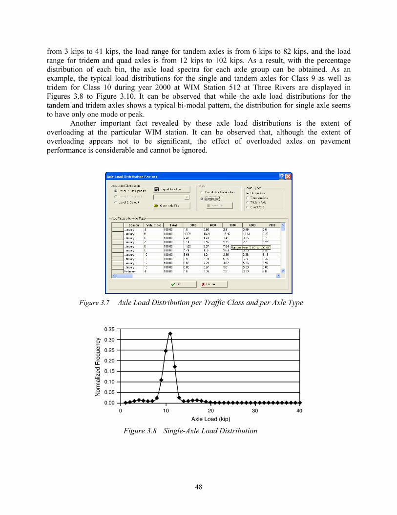
48

from 3 kips to 41 kips, the load range for tandem axles is from 6 kips to 82 kips, and the load range for tridem and quad axles is from 12 kips to 102 kips. As a result, with the percentage distribution of each bin, the axle load spectra for each axle group can be obtained. As an example, the typical load distributions for the single and tandem axles for Class 9 as well as tridem for Class 10 during year 2000 at WIM Station 512 at Three Rivers are displayed in Figures 3.8 to Figure 3.10. It can be observed that while the axle load distributions for the tandem and tridem axles shows a typical bi-modal pattern, the distribution for single axle seems to have only one mode or peak.

Another important fact revealed by these axle load distributions is the extent of overloading at the particular WIM station. It can be observed that, although the extent of overloading appears not to be significant, the effect of overloaded axles on pavement performance is considerable and cannot be ignored.

Figure 3.7 Axle Load Distribution per Traffic Class and per Axle Type

Figure 3.8 Single-Axle Load Distribution

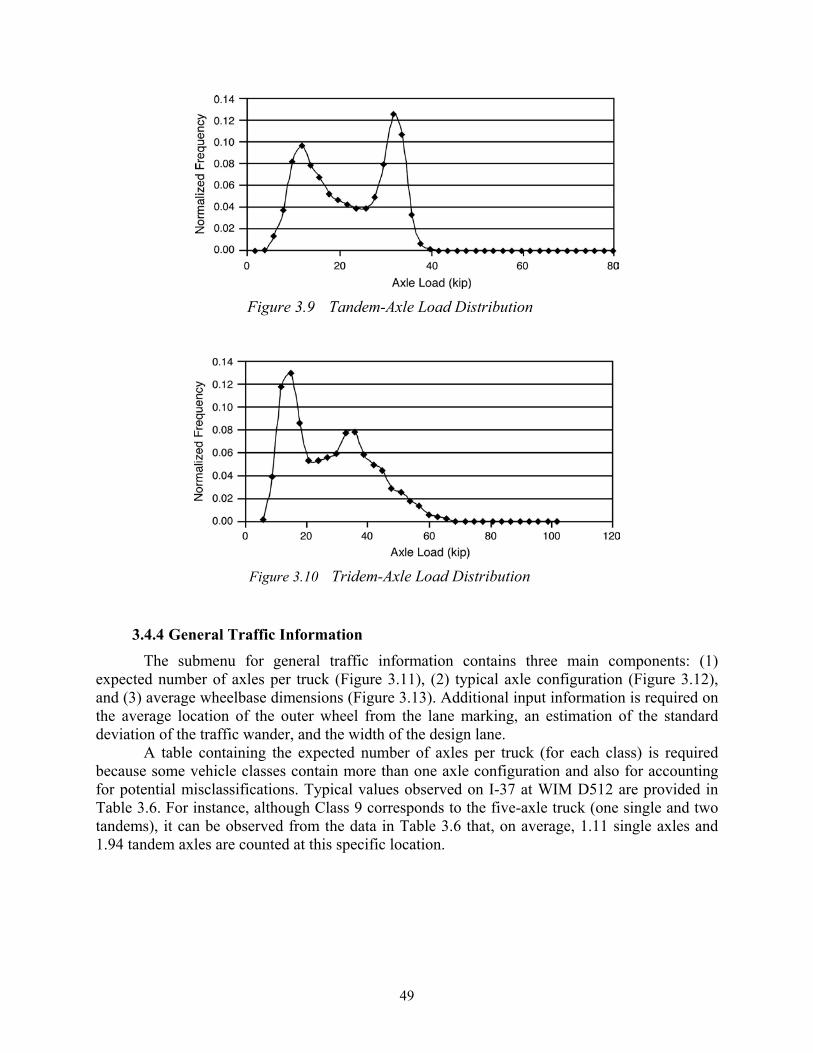
49

Figure 3.9 Tandem-Axle Load Distribution

Figure 3.10 Tridem-Axle Load Distribution

3.4.4 General Traffic Information The submenu for general traffic information contains three main components: (1)

expected number of axles per truck (Figure 3.11), (2) typical axle configuration (Figure 3.12), and (3) average wheelbase dimensions (Figure 3.13). Additional input information is required on the average location of the outer wheel from the lane marking, an estimation of the standard deviation of the traffic wander, and the width of the design lane.

A table containing the expected number of axles per truck (for each class) is required because some vehicle classes contain more than one axle configuration and also for accounting for potential misclassifications. Typical values observed on I-37 at WIM D512 are provided in Table 3.6. For instance, although Class 9 corresponds to the five-axle truck (one single and two tandems), it can be observed from the data in Table 3.6 that, on average, 1.11 single axles and 1.94 tandem axles are counted at this specific location.

50

Table 3.6 Number of Axles per Truck Class Single Tandem Tridem Quad 4 1.41 0.5 0 0 5 2.06 0.07 0 0 6 1.00 1.00 0 0 7 1.00 0 1.00 0 8 2.28 0.72 0 0 9 1.11 1.94 0 0 10 1.00 1.00 0.99 0 11 5.00 0 0 0 12 3.85 1.04 0 0 13 2.75 0.59 0.06 0

Figure 3.11 Screen Showing Expected Number of Axles per Truck

Primarily for the design of jointed hydraulic cement concrete pavements (JCP), additional general traffic inputs are required to characterize the typical spacing between wheels and axles for different trucks. This information consists of the following:

Axle Configuration (Figure 3.12) • Average axle width • Dual tire spacing • Average axle spacing for tandem, tridem, and quads • Average tire pressure

51

Wheelbase Dimensions (Figure 3.13) • Percentage of short, medium, and long wheelbases • Average axle spacing for each group

The complete procedure for obtaining detailed loading information of the traffic expected

on the pavement during its design life can be summarized in the flow chart shown in Figure 3.14.

Figure 3.12 Mean Axle Configuration Parameters

52

Figure 3.13 Mean Wheelbase Dimensions for Short, Medium,

and Long Units

Figure 3.14 Flow Chart of Traffic Input to Obtain Axle Load Spectra

Number of axles per vehicle

Load Distribution for each axle group in each

month

Percentage of each truck class

Monthly Adjustment Factor

Traffic volume forecast for each

class

AADTT of each class

Axle Load Spectra

AADTT

Adjusted AADTT of each class

53

4. Mechanistic Analysis

The mechanistic-empirical design approach proposed in the NCHRP 1-37A Design Guide makes use of a large number of input variables to estimate the performance of a given pavement structure. Those variables include material and structural properties, traffic characteristics, and environmental conditions. Each of those variables is random by nature and incorporates uncertainty into the pavement performance analysis. Due to the running time of the current version of the software (approximately 45 minutes for a four-layer pavement structure with a Pentium 4 processor at 1.7 GHz), the consideration of the effect of each design input variable on performance (full sensitivity analysis) is unfeasible at this time. It was believed, however, that a preliminary sensitivity analysis would be beneficial to identify some of the variables that exert the most significant effect on performance.

The M-E Design Guide software was used to simulate and analyze two pavement structures incorporating local loading patterns and environmental conditions of four typical Texas locations. A relatively light (designed for 1,000,000 ESALs) and a relatively heavy (designed for 6,000,000 ESALs) pavement structures were selected based on information provided by the Design Engineer of the Tyler District. These structures are actual designs based on current design methodology used by the Texas Department of Transportation. Some modifications to these designs were necessary to accommodate the data requirements of the M-E Design Guide. The details of both structures are provided in Table 4.1. It should be noted that the intent of this exercise was to determine sensitivity to traffic variables and not to establish accurate performance predictions.

4.1 Sensitivity Analysis Although numerous failure criteria have been incorporated into the M-E Design Guide,

only fatigue cracking, surface rutting, and roughness progression were evaluated in this analysis. This decision was made because unreasonable performance predictions seem to indicate that some of the transfer functions (performance prediction equations) have not been properly calibrated to Texas conditions.

The performance analysis was carried out in two different stages. During the first part of the analysis, only axle loads were varied, while for the second part only the average annual daily truck traffic (AADTT) was varied. For all analyses a Level 3 design was used: default material properties were used and traffic input was limited to single and tandem axle loads. Since only the effect of axle load was investigated in the first part of the analysis, it was decided to simulate all traffic loads either as single axles or tandem axles of varying loads. In addition, running the software with tridem axle data caused it to freeze on several occasions.

54

Table 4.1 Pavement Structures Used in the Preliminary Analysis Heavy Pavement Property Light Pavement

AC Surface Layer AC 0.35 Poisson's Ratio 0.35

6 Thickness (in.) 1 PG70-22 PG Grade PG70-22

20 Cum.% Retained 3/4 in. 20 30 Cum.% Retained 3/8 in. 30 78 Cum.% Retained # 4 Sieve 78 6 % Passing # 200 Sieve 6

A-1-a Granular Base Layer 1 A-1-a 50,000 Resilient Modulus (psi) 50,000 0.35 Poisson's Ratio 0.35 10 Thickness (in.) 10 1 Plasticity Index, PI 1 3 % Passing # 200 Sieve 3

20 % Passing # 4 Sieve 20 8 D60 8

A-1-b Granular Base Layer 2 A-2-4 75,000 Resilient Modulus (psi) 35,000 0.35 Poisson's Ratio 0.35 10 Thickness (in.) 4 1 Plasticity Index, PI 2 3 % Passing # 200 Sieve 20

40 % Passing # 4 Sieve 80 2 D60 0.1

MH Subgrade MH 12,000 Resilient Modulus (psi) 12,000

0.4 Poisson's Ratio 0.4 20 Plasticity Index, PI 20 75 % Passing # 200 Sieve 75 95 % Passing # 4 Sieve 95

0.01 D60 0.01 Traffic Information

7,000 ADT0 1,500 20 Percentage Trucks 20 2 Growth Factor (Compound) 1.5

6,000,000 Design ESAL 1,000,000 In a first attempt, the properties of commonly used materials based on TxDOT

specifications (TxDOT, 1993) were incorporated into the asphalt mix design. It was observed that some of these values were outside the ranges recommended by the guide. Additionally, the performance predictions were often unreasonable or the program failed to run properly. For this reason, it was decided to alter this approach and to utilize guide default values for material properties in order to be well within the range of the current calibration of the design guide. Hence, in the final run, the pavement sections cannot be considered to be representative of

55

Texas. However, the objective was to evaluate the sensitivity of the results to variables such as axle type, axle load and traffic volume under diverse environmental conditions.

It can be observed from Table 4.1 that for both pavement structures (referred to as heavy and light), the properties of the surface, granular base, and subgrade are similar. The main differences are found in the thickness of the surface layer and the properties of the granular subbase layer, which is the only layer to use different materials for the heavy and light pavements.

The surface layer for both cases is asphalt concrete with a thickness of 6 inches for the heavy pavement and 1 inch for the light pavement. Superpave binder grading PG70-22 was selected to cover the range of environmental conditions simulated across Texas. A Poisson’s ratio of 0.35 was used for both pavement types. The specific asphalt mix gradation is also provided in Table 4.1.

The granular base layer was identical for both heavy and light pavements. Both were composed of Type A-1-a (AASHTO classification) unbound granular material with a layer thickness of 10 inches, a Poisson’s ratio of 0.35, a resilient modulus of 50,000 psi, and a plasticity index (PI) of 1.0. The gradation curve of the base material is also given in Table 4.1.

The granular sub-base used for the heavy pavement consisted of unbound granular material Type A-1-b, while for the light pavement structure, a Type A-2-4 was used instead. Again, the Poisson’s ratio was 0.35 for both, but the heavy pavement layer was 10 inches thick while the light pavement layer was only 4 inches thick. The resilient modulus was also higher for the heavy pavement than the light pavement, i.e., 75,000 and 35,000 psi, respectively. The plasticity index was 1.0 for the heavy pavement and 2.0 for the light pavement.

Finally, the natural soil (or subgrade) was assumed identical for both structures, and it consisted of a silt of high plasticity (MH). The Poisson’s ratio was 0.40 and the resilient modulus was 12,000 psi. All gradations and properties can be found in Table 4.1.

4.1.2 Analysis 1: Effect of Axle Type and Axle Load The first analysis was aimed at assessing the effect of axle type (single or tandem) and

axle load on pavement performance. The heavy pavement was designed for a two-way average annual daily truck traffic (AADTT) of 1,400 standard axles and a compound growth factor of 2.0 percent, while the light pavement was designed for an AADTT of 300 standard axles and a compound growth factor of 1.5 percent. These values remained constant for each simulation while only the axle load was changed. In the axle load distribution factors table, all axle load bins (of the load spectrum) were set to 0 percent except the load of interest for that simulation, which was set to 100 percent.

To simulate single and tandem axles, only one vehicle class was considered in the analysis: Class 10 (according to FHWA’s 2001 Traffic Monitoring Guide), which comprises trucks with single, tandem and tridem axles. For instance, in order to simulate single axles the number of axles per truck (Figure 3.11) is set to 1, 0, 0 for single, tandem and tridem axles respectively. While running the Design Guide program with single and tandem axles produced reasonable performance estimations (discussed in the following sections), running the tridem axle simulations timed out the program or prevented it from being run to completion, indicating a problem with the software. For this reason, only the effect of single and tandem axles only was evaluated in this part of the analysis.

The axle configurations and loads tested are summarized in Table 4.2. Single axle loads ranged from 9 kips to 36 kips while tandem axle loads ranged from 16 kips to 64 kips. All

56

simulations were carried out assuming a water table depth of 100 feet to minimize its influence in the final performance predictions. Environmental information from the following four weather stations was used to represent the typical varying environmental conditions across Texas: Camp Mabry in Austin (AUS), Amarillo International Airport (AMA), El Paso International Airport (ELP) and Houston Intercontinental Airport (HOU).

Table 4.2 Load and Axle Configurations

Single Axle Load (lbs) Tandem Axle Load (lbs)

9,000 16,000 11,000 20,000 14,000 26,000 18,000 32,000 23,000 40,000 29,000 50,000 36,000 64,000

4.1.3 Analysis 2: Effect of Traffic Volume The second part of the analysis assessed the effect of traffic volume on pavement

performance. This was done by varying only the AADTT for each of the four representative locations mentioned in Analysis 1 and for the same two pavement structures as outlined in Table 4.1. Once again, the water table remained at a depth of 100 feet and the traffic growth factors remained at 2.0 percent for heavy pavement and 1.5 percent for light pavement. Table 4.3 outlines the AADTT values used for this analysis. For the heavy pavement the values ranged incrementally from 700 to 2,800 trucks and for the light pavement the values ranged incrementally from 150 to 600 trucks. It should be kept in mind that the AADTT is given in terms of single axles of standard load: 18,000 and 32,000 lbs. for the single and tandem axles, respectively.

Table 4.3 Traffic Volumes Expressed in Terms of AADTT Values Heavy Pavement Light Pavement

700 150 990 212

1400 300 1980 424 2800 600

4.1.4 Performance Results of Analyses 1 and 2

Tables 4.4 through 4.11 summarize the relevant results obtained after running the M-E Design Guide software for Analysis 1, in which only axle type and the axle load varied. In the first column the axle type and axle load are indicated: S for single and D for tandem. The next three columns show the final total rutting, roughness and asphalt-only rutting at the end of the analysis period (20 years). The following three columns show the number of axle load repetitions (or life) to reach different failure criteria. The maximum bottom-up cracking is reported as the

57

number of repetitions necessary to first reach 100 percent surface cracking, as defined in the M-E Design Guide. The 1-inch and 2-inch total rutting are reported similarly as the number of repetitions to first reach 1 and 2 inches of surface rutting, respectively. Since there was the concern that the performance models (or transfer functions) were not calibrated to Texas conditions, it was decided to express all results relative to the performance under the standard axle. Thus, the remaining columns of the tables are designated as “Relative Life” because they either represent the total damage at the end of the analysis period relative to the damage caused by the standard axle (18-kips single axle with dual wheels) or the relative life.

The relative life is the life of the pavement (number of repetitions to reach a given failure criterion) under an axle of a generic load, divided by the life of the pavement under the standard axle load. In this way, the relative life represents the inverse of the load equivalence factor (LEF) or the equivalent damage factor (EDF). For instance, the relative total rutting for the 9-kips single axle load for the Amarillo heavy pavement at the end of the analysis period is 1.505 divided by 2.007. One the other hand, the relative life is obtained as the ratio between 1,782,930 and 511,699 repetitions, when failure is defined as 1 inch of surface rutting. Note also that the upper part of the table contains the data corresponding to single axle loads, denoted as S, while the lower part pertains to tandem axle loads, denoted D. The first load, S09, indicates a 9-kips single axle load, while D32 indicates a 32-kips tandem axle load. In general the results were as expected: (1) as load increases, pavement life shortens at different rates, and (2) as traffic volume increases, life shortens almost linearly.

4.1.5 Results of Analysis 1 The IRI predictions are not relevant in this analysis because pavement roughness reached

a maximum level and then stayed constant. This was attributed to the particular calibration settings for the roughness transfer functions. The surface rutting is higher than expected, but by using the relative analysis approach the problem with the magnitude of the numbers is avoided.

In general the trends are consistent within the heavy pavement models (Tables 4.4 through 4.7). Although the heavy pavement models did not reach 100 percent cracking or 2 inches of rutting for the lighter loads, they still yielded interesting results. The relative total rutting typically increased from 0.7 to 1.15 for the increasing single axle loads and from 0.83 to 1.38 for the tandem axle loads. The relative asphalt concrete (AC) rutting typically exhibited an increase from 0.9 to 1.02 for increasing single axle loads and from 1.16 to 1.33 for the tandem axle loads. The relative cracking, however, decreases from 2.94 to 0.08 for increasing single axle loads and from 2.58 to 0.08 for tandem axle loads. Cracking performance was determined as the number of repetitions to 100 percent surface cracking, so the lighter axle loads should yield a larger number of repetitions than the heavier loads, which explains the decrease in the relative value. The same decreasing trend is exhibited by the relative 1- and 2-inch rutting. This would indicate that the terminal level would not significantly affect the relative performance.

The relative 1-inch rutting decreases from 3.48 to 0.36 for increasing single axle loads and from 2.0 to 0.3 for tandem axle loads. Similarly, the relative 2-inch rutting decreases from 3.05 to 0.44 for increasing single axle loads and from 1.87 to 0.3 for tandem axle loads. All data are presented in Tables 4.4 through 4.7.

Similar to the heavy pavement models, performance trends are consistent within the light pavement models; however, they are not always realistic. These data are summarized in Tables 4.8 through 4.11. For single axle increasing loads, the relative total rutting decreased from 1.04 to 0.83 and from 1.25 to 1.08 for the tandem axle loads. The relative AC rutting exhibited a

58

slight increase, then a decrease after the 14-kip load for the single axle and the 26-kip load for the tandem axle. The values ranged from 0.9 up to 1.0 and down to 0.73 for single axle loads and from 1.2 up to 1.35 and down to 1.0 for tandem axle loads. The relative cracking decreased from 2.28 to 0.56 for single axle loads and from 1.5 to 0.3 for tandem axle loads. The relative ½-inch and ¾-inch rutting exhibited a slight decrease, then an increase after the 18-kip load for the single axle data and after the 32-kip load for the tandem axle data. For the ½-inch rutting, the single axle loads yielded a trend of 1.4 down to 1.0, then back up to 2.2. Similarly, the trend for the tandem axle ½-inch rutting started at 0.9 down to 0.58 and back up to 1.0. The single axle ¾-inch rutting went from 1.0 to 0.8 back up to 2.0, and the tandem axle ¾-inch rutting went from 0.6 to 0.47 up to 0.85.

Table 4.4 Amarillo Heavy Pavement Load Data

Axl

e ty

pe/L

oad

(kip

)

Tota

l Rut

(in.

)

Tota

l IR

I in.

/mile

Subt

otal

AC

Rut

(20y

rs) i

n.

Max

. Bot

tom

Up

Cra

ckin

g,

100%

(#re

ps)

1 in

. Tot

al R

ut (#

reps

)

2 in

. Tot

al R

ut (#

reps

)

Rel

ativ

e Li

fe (T

otal

Rut

)

Rel

ativ

e Li

fe (I

RI)

Rel

ativ

e Li

fe (A

C R

ut)

Rel

ativ

e Li

fe (C

rack

ing)

Rel

ativ

e Li

fe

(1 in

. Tot

al R

ut)

Rel

ativ

e Li

fe

(2 in

. Tot

al R

ut)

S09 1.505 118.9 0.798 ----- 1782930 ----- 0.7499 0.8309 0.9279 ----- 3.4843 ----- S11 1.663 119.2 0.828 ----- 1242110 ----- 0.8286 0.8330 0.9628 ----- 2.4274 ----- S14 1.846 130.2 0.857 ----- 915183 ----- 0.9198 0.9099 0.9965 ----- 1.7885 ----- S18 2.007 143.1 0.86 5200860 511699 5901620 1 1 1 1 1 1 S23 2.147 143.1 0.869 1782930 449349 4749610 1.0698 1 1.0105 0.3428 0.8782 0.8048 S29 2.248 143.1 0.862 701227 242891 3853750 1.1201 1 1.0023 0.1348 0.4747 0.6530 S36 2.367 143.1 0.881 242891 202409 3031180 1.1794 1 1.0244 0.0467 0.3956 0.5136 D16 1.792 118.9 1.016 ----- 1023010 ----- 0.8929 0.8309 1.1814 ----- 1.9992 ----- D20 1.998 119.3 1.076 ----- 722286 ----- 0.9955 0.8337 1.2512 ----- 1.4115 ----- D26 2.223 136.2 1.112 ----- 469995 4200420 1.1076 0.9518 1.2930 ----- 0.9185 0.7117 D32 2.364 143.1 1.109 5461040 449349 3488710 1.1779 1 1.2895 1.0500 0.8782 0.5911 D40 2.516 143.1 1.122 2038230 242891 2635400 1.2536 1 1.3047 0.3919 0.4747 0.4466 D50 2.634 143.1 1.116 743344 222650 2084730 1.3124 1 1.2977 0.1429 0.4351 0.3532 D64 2.78 143.1 1.126 263537 161928 1646160 1.3852 1 1.3093 0.0507 0.3165 0.2789

59

Table 4.5 Austin Heavy Pavement Load Data A

xle

type

/Loa

d (k

ip)

Tota

l Rut

(in.

)

Tota

l IR

I in.

/mile

Subt

otal

AC

Rut

(20y

rs) i

n.

Max

. Bot

tom

Up

Cra

ckin

g,

100%

(#re

ps)

1 in

. Tot

al R

ut (#

reps

)

2 in

. Tot

al R

ut (#

reps

)

Rel

ativ

e Li

fe (T

otal

Rut

)

Rel

ativ

e Li

fe (I

RI)

Rel

ativ

e Li

fe (A

C R

ut)

Rel

ativ

e Li

fe (C

rack

ing)

Rel

ativ

e Li

fe

(1 in

. Tot

al R

ut)

Rel

ativ

e Li

fe

(2 in

. Tot

al R

ut)

S09 2.554 91.3 1.144 ----- 490640 2931000 0.7326 0.7939 0.9094 ----- 2.2036 2.8651 S11 2.844 102.8 1.191 ----- 387412 2084730 0.8158 0.8939 0.9467 ----- 1.7400 2.0378 S14 3.179 115 1.241 5200860 242891 1487490 0.9119 1 0.9865 2.8802 1.0909 1.4540 S18 3.486 115 1.258 1805720 222650 1023010 1 1 1 1 1 1 S23 3.737 115 1.268 722286 202409 722286 1.0720 1 1.0079 0.4000 0.9091 0.7060 S29 3.896 115 1.263 263537 141687 722286 1.1176 1 1.0040 0.1459 0.6364 0.7060 S36 3.984 115 1.285 182168 101205 595934 1.1429 1 1.0215 0.1009 0.4545 0.5825 D16 2.992 91.2 1.46 ----- 284183 1828970 0.8583 0.7930 1.1606 ----- 1.2764 1.7878 D20 3.363 104.1 1.554 ----- 242891 1242110 0.9647 0.9052 1.2353 ----- 1.0909 1.2142 D26 3.786 115 1.627 4527320 222650 936663 1.0861 1 1.2933 2.5072 1 0.9156 D32 4.064 115 1.638 1852220 202409 743344 1.1658 1 1.3021 1.0258 0.9091 0.7266 D40 4.347 115 1.663 764824 161928 574875 1.2470 1 1.3219 0.4236 0.7273 0.5619 D50 4.54 115 1.66 366766 101205 469995 1.3024 1 1.3196 0.2031 0.4545 0.4594 D64 4.671 115 1.675 202409 60723 387412 1.3399 1 1.3315 0.1121 0.2727 0.3787

Table 4.6 El Paso Heavy Pavement Load Data

Axl

e ty

pe/L

oad

(kip

)

Tota

l Rut

(in.

)

Tota

l IR

I in.

/mile

Subt

otal

AC

Rut

(20y

rs) i

n.

Max

. Bot

tom

Up

Cra

ckin

g,

100%

(#re

ps)

1 in

. Tot

al R

ut (#

reps

)

2 in

. Tot

al R

ut (#

reps

)

Rel

ativ

e Li

fe (T

otal

Rut

)

Rel

ativ

e Li

fe (I

RI)

Rel

ativ

e Li

fe (A

C R

ut)

Rel

ativ

e Li

fe (C

rack

ing)

Rel

ativ

e Li

fe

(1 in

. Tot

al R

ut)

Rel

ativ

e Li

fe

(2 in

. Tot

al R

ut)

S09 2.396 96 1.009 ----- 469995 3360360 0.7303 0.8007 0.9377 ----- 2.3220 2.7539 S11 2.67 103.1 1.042 ----- 325474 2393500 0.8138 0.8599 0.9684 ----- 1.6080 1.9616 S14 2.992 119.9 1.079 5872130 222650 1691750 0.9119 1 1.0028 2.9483 1.1000 1.3865 S18 3.281 119.9 1.076 1991730 202409 1220200 1 1 1 1 1 1 S23 3.528 119.9 1.077 701227 182168 893703 1.0753 1 1.0009 0.3521 0.9000 0.7324 S29 3.678 119.9 1.057 242891 121446 680168 1.1210 1 0.9823 0.1219 0.6000 0.5574 S36 3.759 119.9 1.062 161928 80964 532758 1.1457 1 0.9870 0.0813 0.4000 0.4366 D16 2.796 96 1.288 ----- 263537 2108440 0.8522 0.8007 1.1970 ----- 1.3020 1.7279 D20 3.149 104 1.366 ----- 222650 1487490 0.9598 0.8674 1.2695 ----- 1.1000 1.2191 D26 3.549 119.9 1.416 5144180 202409 979623 1.0817 1 1.3160 2.5828 1 0.8028 D32 3.816 119.9 1.416 2061480 182168 722286 1.1631 1 1.3160 1.0350 0.9000 0.5919 D40 4.08 119.9 1.42 764824 141687 511699 1.2435 1 1.3197 0.3840 0.7000 0.4194 D50 4.271 119.9 1.409 263537 80964 449349 1.3017 1 1.3095 0.1323 0.4000 0.3683 D64 4.383 119.9 1.396 161928 60723 366766 1.3359 1 1.2974 0.0813 0.3000 0.3006

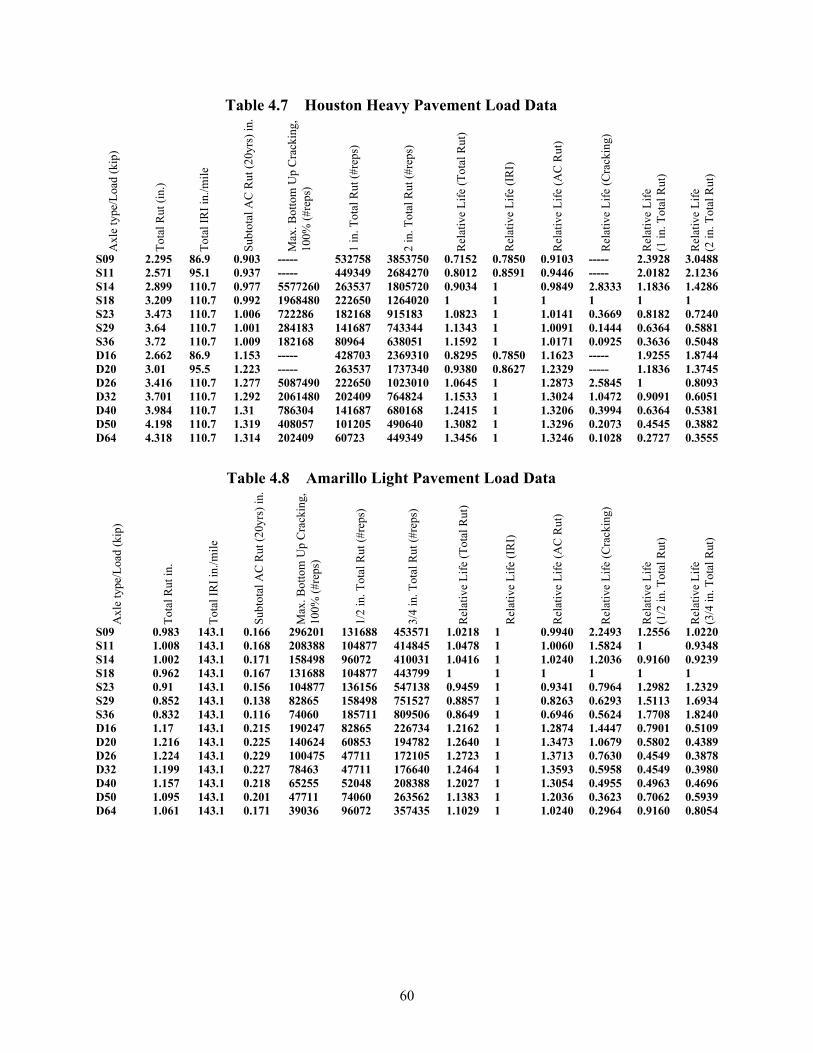
60

Table 4.7 Houston Heavy Pavement Load Data A

xle

type

/Loa

d (k

ip)

Tota

l Rut

(in.

)

Tota

l IR

I in.

/mile

Subt

otal

AC

Rut

(20y

rs) i

n.

Max

. Bot

tom

Up

Cra

ckin

g,

100%

(#re

ps)

1 in

. Tot

al R

ut (#

reps

)

2 in

. Tot

al R

ut (#

reps

)

Rel

ativ

e Li

fe (T

otal

Rut

)

Rel

ativ

e Li

fe (I

RI)

Rel

ativ

e Li

fe (A

C R

ut)

Rel

ativ

e Li

fe (C

rack

ing)

Rel

ativ

e Li

fe

(1 in

. Tot

al R

ut)

Rel

ativ

e Li

fe

(2 in

. Tot

al R

ut)

S09 2.295 86.9 0.903 ----- 532758 3853750 0.7152 0.7850 0.9103 ----- 2.3928 3.0488 S11 2.571 95.1 0.937 ----- 449349 2684270 0.8012 0.8591 0.9446 ----- 2.0182 2.1236 S14 2.899 110.7 0.977 5577260 263537 1805720 0.9034 1 0.9849 2.8333 1.1836 1.4286 S18 3.209 110.7 0.992 1968480 222650 1264020 1 1 1 1 1 1 S23 3.473 110.7 1.006 722286 182168 915183 1.0823 1 1.0141 0.3669 0.8182 0.7240 S29 3.64 110.7 1.001 284183 141687 743344 1.1343 1 1.0091 0.1444 0.6364 0.5881 S36 3.72 110.7 1.009 182168 80964 638051 1.1592 1 1.0171 0.0925 0.3636 0.5048 D16 2.662 86.9 1.153 ----- 428703 2369310 0.8295 0.7850 1.1623 ----- 1.9255 1.8744 D20 3.01 95.5 1.223 ----- 263537 1737340 0.9380 0.8627 1.2329 ----- 1.1836 1.3745 D26 3.416 110.7 1.277 5087490 222650 1023010 1.0645 1 1.2873 2.5845 1 0.8093 D32 3.701 110.7 1.292 2061480 202409 764824 1.1533 1 1.3024 1.0472 0.9091 0.6051 D40 3.984 110.7 1.31 786304 141687 680168 1.2415 1 1.3206 0.3994 0.6364 0.5381 D50 4.198 110.7 1.319 408057 101205 490640 1.3082 1 1.3296 0.2073 0.4545 0.3882 D64 4.318 110.7 1.314 202409 60723 449349 1.3456 1 1.3246 0.1028 0.2727 0.3555

Table 4.8 Amarillo Light Pavement Load Data

Axl

e ty

pe/L

oad

(kip

)

Tota

l Rut

in.

Tota

l IR

I in.

/mile

Subt

otal

AC

Rut

(20y

rs) i

n.

Max

. Bot

tom

Up

Cra

ckin

g,

100%

(#re

ps)

1/2

in. T

otal

Rut

(#re

ps)

3/4

in. T

otal

Rut

(#re

ps)

Rel

ativ

e Li

fe (T

otal

Rut

)

Rel

ativ

e Li

fe (I

RI)

Rel

ativ

e Li

fe (A

C R

ut)

Rel

ativ

e Li

fe (C

rack

ing)

Rel

ativ

e Li

fe

(1/2

in. T

otal

Rut

)

Rel

ativ

e Li

fe

(3/4

in. T

otal

Rut

)

S09 0.983 143.1 0.166 296201 131688 453571 1.0218 1 0.9940 2.2493 1.2556 1.0220 S11 1.008 143.1 0.168 208388 104877 414845 1.0478 1 1.0060 1.5824 1 0.9348 S14 1.002 143.1 0.171 158498 96072 410031 1.0416 1 1.0240 1.2036 0.9160 0.9239 S18 0.962 143.1 0.167 131688 104877 443799 1 1 1 1 1 1 S23 0.91 143.1 0.156 104877 136156 547138 0.9459 1 0.9341 0.7964 1.2982 1.2329 S29 0.852 143.1 0.138 82865 158498 751527 0.8857 1 0.8263 0.6293 1.5113 1.6934 S36 0.832 143.1 0.116 74060 185711 809506 0.8649 1 0.6946 0.5624 1.7708 1.8240 D16 1.17 143.1 0.215 190247 82865 226734 1.2162 1 1.2874 1.4447 0.7901 0.5109 D20 1.216 143.1 0.225 140624 60853 194782 1.2640 1 1.3473 1.0679 0.5802 0.4389 D26 1.224 143.1 0.229 100475 47711 172105 1.2723 1 1.3713 0.7630 0.4549 0.3878 D32 1.199 143.1 0.227 78463 47711 176640 1.2464 1 1.3593 0.5958 0.4549 0.3980 D40 1.157 143.1 0.218 65255 52048 208388 1.2027 1 1.3054 0.4955 0.4963 0.4696 D50 1.095 143.1 0.201 47711 74060 263562 1.1383 1 1.2036 0.3623 0.7062 0.5939 D64 1.061 143.1 0.171 39036 96072 357435 1.1029 1 1.0240 0.2964 0.9160 0.8054

61

Table 4.9 Austin Light Pavement Load Data A

xle

type

/Loa

d (k

ip)

Tota

l Rut

in.

Tota

l IR

I in.

/mile

Subt

otal

AC

Rut

(20y

rs) i

n.

Max

. Bot

tom

Up

Cra

ckin

g,

100%

(#re

ps)

1/2

in. T

otal

Rut

(#re

ps)

3/4

in. T

otal

Rut

(#re

ps)

Rel

ativ

e Li

fe (T

otal

Rut

)

Rel

ativ

e Li

fe (I

RI)

Rel

ativ

e Li

fe (A

C R

ut)

Rel

ativ

e Li

fe (C

rack

ing)

Rel

ativ

e Li

fe

(1/2

in. T

otal

Rut

)

Rel

ativ

e Li

fe

(3/4

in. T

otal

Rut

)

S09 1.266 115 0.213 185711 69658 212924 1.0437 1 0.9907 2.2411 1.3383 1.0445 S11 1.292 115 0.216 140624 56451 190247 1.0651 1 1.0047 1.6970 1.0846 0.9333 S14 1.276 115 0.22 109345 52048 176640 1.0519 1 1.0233 1.3196 1 0.8665 S18 1.213 115 0.215 82865 52048 203853 1 1 1 1 1 1 S23 1.141 115 0.202 69658 69658 254355 0.9406 1 0.9395 0.8406 1.3383 1.2477 S29 1.066 115 0.178 65255 91670 343207 0.8788 1 0.8279 0.7875 1.7613 1.6836 S36 1.017 115 0.151 56451 109345 414845 0.8384 1 0.7023 0.6812 2.1008 2.0350 D16 1.518 115 0.276 118282 47711 127219 1.2514 1 1.2837 1.4274 0.9167 0.6241 D20 1.569 115 0.288 87267 39036 104877 1.2935 1 1.3395 1.0531 0.7500 0.5145 D26 1.571 115 0.295 65255 30361 96072 1.2951 1 1.3721 0.7875 0.5833 0.4713 D32 1.526 115 0.292 52048 30361 96072 1.2580 1 1.3581 0.6281 0.5833 0.4713 D40 1.465 115 0.281 39036 30361 109345 1.2077 1 1.3070 0.4711 0.5833 0.5364 D50 1.378 115 0.26 30361 43373 136156 1.1360 1 1.2093 0.3664 0.8333 0.6679 D64 1.313 115 0.223 26024 56451 172105 1.0824 1 1.0372 0.3141 1.0846 0.8443

Table 4.10 El Paso Light Pavement Load Data

Axl

e ty

pe/L

oad

(kip

)

Tota

l Rut

in.

Tota

l IR

I in.

/mile

Subt

otal

AC

Rut

(20y

rs) i

n.

Max

. Bot

tom

Up

Cra

ckin

g,

100%

(#re

ps)

1/2

in. T

otal

Rut

(#re

ps)

3/4

in. T

otal

Rut

(#re

ps)

Rel

ativ

e Li

fe (T

otal

Rut

)

Rel

ativ

e Li

fe (I

RI)

Rel

ativ

e Li

fe (A

C R

ut)

Rel

ativ

e Li

fe (C

rack

ing)

Rel

ativ

e Li

fe

(1/2

in. T

otal

Rut

)

Rel

ativ

e Li

fe

(3/4

in. T

otal

Rut

)

S09 1.254 119.9 0.2 199317 69658 217527 1.0433 1 0.9852 2.2840 1.3383 1.0671 S11 1.281 119.9 0.204 149561 56451 190247 1.0657 1 1.0049 1.7138 1.0846 0.9333 S14 1.266 119.9 0.207 113814 52048 176640 1.0532 1 1.0197 1.3042 1 0.8665 S18 1.202 119.9 0.203 87267 52048 203853 1 1 1 1 1 1 S23 1.131 119.9 0.191 74060 69658 258959 0.9409 1 0.9409 0.8487 1.3383 1.2703 S29 1.057 119.9 0.168 65255 87267 352692 0.8794 1 0.8276 0.7478 1.6767 1.7301 S36 1.009 119.9 0.142 60853 109345 419658 0.8394 1 0.6995 0.6973 2.1008 2.0586 D16 1.501 119.9 0.259 131688 56451 122751 1.2488 1 1.2759 1.5090 1.0846 0.6022 D20 1.554 119.9 0.271 91670 39036 104877 1.2928 1 1.3350 1.0505 0.7500 0.5145 D26 1.556 119.9 0.278 69658 30361 91670 1.2945 1 1.3695 0.7982 0.5833 0.4497 D32 1.511 119.9 0.275 56451 30361 96072 1.2571 1 1.3547 0.6469 0.5833 0.4713 D40 1.45 119.9 0.265 43373 30361 109345 1.2063 1 1.3054 0.4970 0.5833 0.5364 D50 1.365 119.9 0.246 34699 43373 131688 1.1356 1 1.2118 0.3976 0.8333 0.6460 D64 1.302 119.9 0.21 26024 56451 176640 1.0832 1 1.0345 0.2982 1.0846 0.8665

62

Table 4.11 Houston Light Pavement Load Data A

xle

type

/Loa

d (k

ip)

Tota

l Rut

in.

Tota

l IR

I in.

/mile

Subt

otal

AC

Rut

(20y

rs) i

n.

Max

. Bot

tom

Up

Cra

ckin

g,

100%

(#re

ps)

1/2

in. T

otal

Rut

(#re

ps)

3/4

in. T

otal

Rut

(#re

ps)

Rel

ativ

e Li

fe (T

otal

Rut

)

Rel

ativ

e Li

fe (I

RI)

Rel

ativ

e Li

fe (A

C R

ut)

Rel

ativ

e Li

fe (C

rack

ing)

Rel

ativ

e Li

fe

(1/2

in. T

otal

Rut

)

Rel

ativ

e Li

fe

(3/4

in. T

otal

Rut

)

S09 1.234 110.8 0.181 181176 74060 226734 1.0405 1 0.9628 2.1864 1.4229 1.0649 S11 1.261 110.8 0.185 136156 60853 199317 1.0632 1 0.9840 1.6431 1.1692 0.9361 S14 1.246 110.8 0.19 104877 52048 185711 1.0506 1 1.0106 1.2656 1 0.8722 S18 1.186 110.8 0.188 82865 52048 212924 1 1 1 1 1 1 S23 1.118 110.8 0.18 69658 69658 268166 0.9427 1 0.9574 0.8406 1.3383 1.2594 S29 1.049 110.8 0.162 65255 91670 362178 0.8845 1 0.8617 0.7875 1.7613 1.7010 S36 1.004 110.8 0.139 60853 113814 429286 0.8465 1 0.7394 0.7344 2.1867 2.0161 D16 1.476 110.8 0.234 113814 47711 131688 1.2445 1 1.2447 1.3735 0.9167 0.6185 D20 1.526 110.8 0.245 87267 39036 109345 1.2867 1 1.3032 1.0531 0.7500 0.5135 D26 1.529 110.8 0.254 60853 30361 100475 1.2892 1 1.3511 0.7344 0.5833 0.4719 D32 1.487 110.8 0.254 52048 30361 100475 1.2538 1 1.3511 0.6281 0.5833 0.4719 D40 1.431 110.8 0.248 39036 34699 113814 1.2066 1 1.3191 0.4711 0.6667 0.5345 D50 1.35 110.8 0.233 34699 43373 140624 1.1383 1 1.2394 0.4187 0.8333 0.6604 D64 1.292 110.8 0.203 26024 56451 181176 1.0894 1 1.0798 0.3141 1.0846 0.8509

4.1.6 Results of Analysis 2 Tables 4.12 through 4.19 represent the data collected from the second analysis in which

the traffic volume (expressed in AADTT) was varied. The procedures for obtaining these values are similar to those in Analysis 1; the difference is introduced in the relative data. All relative values are compared with those from the prior analysis at the 18-kip single axle load level. For instance, for the AADTT of 700 in Table 4.12, the relative total rutting is 1.863 divided by 2.007 (the value for the total rutting at the 18-kip load from Table 4.4). This technique was used because the 18-kip load in the first analysis had an AADTT of 1,400 for the heavy pavement and 300 for the light pavement, and this analysis brings together the load and the volume of traffic. As during Analysis 1, the roughness results show some unreasonable trends.

The AADTT data for the heavy pavement were not as consistent as those of the light pavement. In general, the relative total rutting and the relative AC rutting consistently increased from 0.93 to 1.44 and from 0.9 to 1.6, respectively. Typically, the relative cracking increased from 0.7 to 0.75, but some results fluctuated. Similarly, the relative 1-inch rutting results fluctuated as well, but increased in the range of 0.5 to 0.9. The relative 2-inch rutting results typically decreased from 0.6 to 0.52, but some were inconsistent and increased from 0.6 to 0.75. A summary of all results can be seen in Tables 4.12 through 4.15.

The AADTT data for the light pavement are more consistent than the data for the heavy pavement. The relative total rutting increased from 1.2 to 1.75 and the relative AC rutting increased from 0.9 to 1.59. The relative cracking increased from 0.6 to 0.84, but the maximum value was typically at an AADTT of 424; the final value at an AADTT of 600 was always lower. The only inconsistencies came with the relative ½-inch rutting, which was constant (close to 0.3), despite some minor fluctuations. The relative ¾-inch rutting consistently increased from 0.23 to 0.38. The only exception is Amarillo for an AADTT of 600 where rutting seems to decrease for no logical reason (Table 4.16).

63

Table 4.12 Amarillo Heavy Pavement AADTT Data A

AD

TT

Tota

l Rut

in.

Tota

l IR

I in.

/mile

Subt

otal

AC

Rut

in.

Max

. Bot

tom

Up

Cra

ckin

g, 1

00%

(#

reps

)

1/2

in. T

otal

Rut

(#

reps

)

3/4

in. T

otal

Rut

(#

reps

)

Rel

ativ

e To

tal R

ut

Rel

ativ

e IR

I

Rel

ativ

e A

C R

ut

Rel

ativ

e C

rack

ing

Rel

ativ

e 1/

2 in

. To

tal R

ut

Rel

ativ

e 3/

4 in

. To

tal R

ut

700 1.863 143.1 0.771 ----- 371672 ----- 0.9283 1 0.8965 ----- 0.7263 ----- 990 2.081 143.1 0.892 3698200 332353 3677750 1.0369 1 1.0372 0.7111 0.6495 0.6232 1400 2.324 143.1 1.031 3775190 428703 3540050 1.1579 1 1.1988 0.7259 0.8378 0.5998 1980 2.595 143.1 1.192 3727210 314891 3350890 1.2930 1 1.3860 0.7167 0.6154 0.5678 2800 2.899 143.1 1.379 3611440 404819 3109960 1.4444 1 1.6035 0.6944 0.7911 0.5270

Table 4.13 Austin Heavy Pavement AADTT Data

AA

DTT

Tota

l Rut

in.

Tota

l IR

I in.

/mile

Subt

otal

AC

Rut

in.

Max

. Bot

tom

Up

Cra

ckin

g, 1

00%

(#

reps

)

1/2

in. T

otal

Rut

(#

reps

)

3/4

in. T

otal

Rut

(#

reps

)

Rel

ativ

e To

tal R

ut

Rel

ativ

e IR

I

Rel

ativ

e A

C R

ut

Rel

ativ

e C

rack

ing

Rel

ativ

e 1/

2 in

. To

tal R

ut

Rel

ativ

e 3/

4 in

. To

tal R

ut

700 3.236 115 1.128 1281420 111325 632008 0.9283 1 0.8967 0.7096 0.5000 0.6178 990 3.603 115 1.305 1293350 143132 692733 1.0336 1 1.0374 0.7163 0.6429 0.6772 1400 4.005 115 1.509 1264020 182168 743344 1.1489 1 1.1995 0.7000 0.8182 0.7266 1980 4.448 115 1.744 1385470 200385 723689 1.2760 1 1.3863 0.7673 0.9000 0.7074 2800 4.936 115 2.017 1486690 202409 774823 1.4159 1 1.6033 0.8233 0.9091 0.7574

Table 4.14 El Paso Heavy Pavement AADTT Data

AA

DTT

Tota

l Rut

in.

Tota

l IR

I in.

/mile

Subt

otal

AC

Rut

in.

Max

. Bot

tom

Up

Cra

ckin

g, 1

00%

(#

reps

)

1/2

in. T

otal

Rut

(#

reps

)

3/4

in. T

otal

Rut

(#

reps

)

Rel

ativ

e To

tal R

ut

Rel

ativ

e IR

I

Rel

ativ

e A

C R

ut

Rel

ativ

e C

rack

ing

Rel

ativ

e 1/

2 in

. To

tal R

ut

Rel

ativ

e 3/

4 in

. To

tal R

ut

700 3.049 119.9 0.966 1440830 111325 754920 0.9293 1 0.8978 0.7234 0.5500 0.6187 990 3.39 119.9 1.117 1441320 143132 707922 1.0332 1 1.0381 0.7237 0.7071 0.5802 1400 3.762 119.9 1.292 1465140 161928 701227 1.1466 1 1.2007 0.7356 0.8000 0.5747 1980 4.17 119.9 1.494 1415840 171759 664707 1.2710 1 1.3885 0.7109 0.8486 0.5448 2800 4.617 119.9 1.727 1444570 121446 692240 1.4072 1 1.6050 0.7253 0.6000 0.5673

Table 4.15 Houston Heavy Pavement AADTT Data

AA

DTT

Tota

l Rut

in.

Tota

l IR

I in.

/mile

Subt

otal

AC

Rut

in.

Max

. Bot

tom

Up

Cra

ckin

g, 1

00%

(#

reps

)

1/2

in. T

otal

Rut

(#

reps

)

3/4

in. T

otal

Rut

(#

reps

)

Rel

ativ

e To

tal R

ut

Rel

ativ

e IR

I

Rel

ativ

e A

C R

ut

Rel

ativ

e C

rack

ing

Rel

ativ

e 1/

2 in

. To

tal R

ut

Rel

ativ

e 3/

4 in

. To

tal R

ut

700 2.978 110.7 0.887 1416150 121446 811683 0.9280 1 0.8942 0.7194 0.5455 0.6421 990 3.307 110.7 1.026 1441320 157446 769895 1.0305 1 1.0343 0.7322 0.7071 0.6091 1400 3.665 110.7 1.186 1487490 182168 743344 1.1421 1 1.1956 0.7557 0.8182 0.5881 1980 4.057 110.7 1.371 1446830 171759 813038 1.2643 1 1.3821 0.7350 0.7714 0.6432 2800 4.486 110.7 1.585 1486690 161928 898698 1.3979 1 1.5978 0.7552 0.7273 0.7110

64

Table 4.16 Amarillo Light Pavement AADTT Data A

AD

TT

Tota

l Rut

in.

Tota

l IR

I in.

/mile

Subt

otal

AC

Rut

in.

Max

. Bot

tom

Up

Cra

ckin

g, 1

00%

(#

reps

)

1/2

in. T

otal

Rut

(#

reps

)

3/4

in. T

otal

Rut

(#

reps

)

Rel

ativ

e To

tal R

ut

Rel

ativ

e IR

I

Rel

ativ

e A

C R

ut

Rel

ativ

e C

rack

ing

Rel

ativ

e 1/

2 in

. To

tal R

ut

Rel

ativ

e 3/

4 in

. To

tal R

ut

150 1.166 143.1 0.149 79249 28225 104194 1.2121 1 0.8922 0.6018 0.2691 0.2348 212 1.274 143.1 0.172 93059 30651 112005 1.3243 1 1.0299 0.7067 0.2923 0.2524 300 1.391 143.1 0.199 91670 30361 131688 1.4459 1 1.1916 0.6961 0.2895 0.2967 424 1.517 143.1 0.23 98450 24521 135782 1.5769 1 1.3772 0.7476 0.2338 0.3060 600 1.653 143.1 0.266 95422 26024 121706 1.7183 1 1.5928 0.7246 0.2481 0.2742

Table 4.17 Austin Light Pavement AADTT Data

AA

DTT

Tota

l Rut

in.

Tota

l IR

I in.

/mile

Subt

otal

AC

Rut

in.

Max

. Bot

tom

Up

Cra

ckin

g, 1

00%

(#

reps

)

1/2

in. T

otal

Rut

(#

reps

)

3/4

in. T

otal

Rut

(#

reps

)

Rel

ativ

e To

tal R

ut

Rel

ativ

e IR

I

Rel

ativ

e A

C R

ut

Rel

ativ

e C

rack

ing

Rel

ativ

e 1/

2 in

. To

tal R

ut

Rel

ativ

e 3/

4 in

. To

tal R

ut

150 1.498 115 0.191 56907 17349 54673 1.2350 1 0.8884 0.6867 0.3333 0.2682 212 1.638 115 0.221 58558 18390 58558 1.3504 1 1.0279 0.7067 0.3533 0.2873 300 1.789 115 0.255 65255 17349 60853 1.4749 1 1.1860 0.7875 0.3333 0.2985 424 1.95 115 0.295 61301 18390 67431 1.6076 1 1.3721 0.7398 0.3533 0.3308 600 2.124 115 0.341 60723 17349 69398 1.7510 1 1.5860 0.7328 0.3333 0.3404

Table 4.18 El Paso Light Pavement AADTT Data

AA

DTT

Tota

l Rut

in.

Tota

l IR

I in.

/mile

Subt

otal

AC

Rut

in.

Max

. Bot

tom

Up

Cra

ckin

g, 1

00%

(#

reps

)

1/2

in. T

otal

Rut

(#

reps

)

3/4

in. T

otal

Rut

(#

reps

)

Rel

ativ

e To

tal R

ut

Rel

ativ

e IR

I

Rel

ativ

e A

C R

ut

Rel

ativ

e C

rack

ing

Rel

ativ

e 1/

2 in

. To

tal R

ut

Rel

ativ

e 3/

4 in

. To

tal R

ut

150 1.486 119.9 0.18 59141 17349 54673 1.2363 1 0.8867 0.6777 0.3333 0.2682 212 1.624 119.9 0.208 58558 18390 58558 1.3511 1 1.0246 0.6710 0.3533 0.2873 300 1.773 119.9 0.24 69658 21687 60853 1.4750 1 1.1823 0.7982 0.4167 0.2985 424 1.932 119.9 0.278 73561 18390 67431 1.6073 1 1.3695 0.8429 0.3533 0.3308 600 2.103 119.9 0.322 69398 17349 78072 1.7496 1 1.5862 0.7952 0.3333 0.3830

Table 4.19 Houston Light Pavement AADTT Data

AA

DTT

Tota

l Rut

in.

Tota

l IR

I in.

/mile

Subt

otal

AC

Rut

in.

Max

. Bot

tom

Up

Cra

ckin

g, 1

00%

(#

reps

)

1/2

in. T

otal

Rut

(#

reps

)

3/4

in. T

otal

Rut

(#

reps

)

Rel

ativ

e To

tal R

ut

Rel

ativ

e IR

I

Rel

ativ

e A

C R

ut

Rel

ativ

e C

rack

ing

Rel

ativ

e 1/

2 in

. To

tal R

ut

Rel

ativ

e 3/

4 in

. To

tal R

ut

150 1.473 110.8 0.167 56907 17349 56907 1.2420 1 0.8883 0.6867 0.3333 0.2673 212 1.61 110.8 0.193 55447 18390 61669 1.3575 1 1.0266 0.6691 0.3533 0.2896 300 1.756 110.8 0.223 65255 17349 60853 1.4806 1 1.1862 0.7875 0.3333 0.2858 424 1.912 110.8 0.257 67431 18390 67431 1.6121 1 1.3670 0.8137 0.3533 0.3167 600 2.08 110.8 0.298 60723 17349 69398 1.7538 1 1.5851 0.7328 0.3333 0.3259

65

The Design Guide software was used for a two-part analysis of data generated from models of heavy and light pavements in four Texas locations. The first analysis produced results of performance as affected by axle configuration and loads while the second analysis produced results relating to the effect of traffic volume.

4.2 Results of the Sensitivity Analysis A graphical summary of the results reported in the previous sections is provided in

Appendix A. Appendix A contains a number of plots representing the relative life of the light and heavy pavement structures as a function of the axle load. Figures are provided for single and tandem axles for the four environmental conditions considered (i.e., Amarillo, Austin, El Paso and Houston). Only the relative life in terms of surface rutting and fatigue cracking are provided because some of the other results were not considered accurate for Texas conditions.

It should be noted that the relative life represents the inverse of the load equivalency factor (LEF) or the equivalent damage factor (EDF). One of the most common approaches to estimate LEFs is by the application of the so-called power law, which represents the value of LEF as a function of the axle load for different axle configurations according to the following expression:

α

⎟⎟⎠

⎞⎜⎜⎝

⎛=

kLLEF

18 (4.1)

Where, LEF : load equivalency factor L : axle load in kips k : parameter that depends on axle configuration α : exponent of the power law

The parameter k takes on different values for single, tandem, tridem, and quad axles. In the case of single axles with dual wheels, k = 1.0. For other axle configurations, however, different authors recommend different values. The exponent α represents the sensitivity of the pavement structure to axle load increase. Commonly used values are between 3.8 and 4.2, but extensive research has shown that this value should vary over a wider range based on pavement characteristics and failure criteria. The regression equations accompanying each plot in Appendix A capture the estimated exponent in each case. A summary of the estimated exponents is given in Table 4.20.

Table 4.20 Summary of Exponents of the Power Law Rutting Cracking Location Structure Single Tandem Single Tandem

Light -0.34 -0.14 0.97 1.14 AMA Heavy 1.59 1.33 4.38 4.39 Light -0.40 -0.11 0.84 1.12 AUS Heavy 1.08 1.04 3.66 3.47 Light -0.38 0.03 0.86 1.13 ELP Heavy 1.12 1.05 3.94 3.98 Light -0.37 -0.13 0.78 1.05 HOU Heavy 1.31 1.24 3.72 3.58

66

When rutting failure is considered for the heavy pavement structure, the average exponents of the power law were 1.28 and 1.17 for single and tandem axles, respectively. When fatigue cracking was considered as the dominant failure mechanism, the exponents were 3.93 and 3.86, respectively. This finding supports previous research showing that different exponents should be determined for different failure criteria and different axle configurations. In addition, the absolute values are consistent with previous research. Hence, in terms of relative performance, the M-E Design Guide seems to yield sensitive and reasonable results.

The results for the case of the light pavement structures are interesting: the rutting life of the pavements seems to increase as the axle load increases for both the single and tandem axle. This is represented by the negative exponents in Table 4.20. In the case of fatigue cracking, pavement life increases but at a significantly lower rate than that for the heavy pavement. The average exponents are 0.86 and 1.11 for the single and tandem axle, respectively. This means that the relationship between axle load increase and damage is almost linear.

The fact that light pavement is less sensitive to overloading than heavy pavement (although counterintuitive) can be explained by the fact that the selected heavy structure has a thickness above the critical value, while the surface thickness of the light pavement structure is below the critical value. Recall that critical thickness value is defined as the surface thickness that results in most pavement distress.

The analysis on the effect of traffic volume indicated that there is an approximated linear relationship between AADTT and pavement life. This fact supports the principle that a pavement designed to fail after twenty years with an AADTT of 1,000 vehicles would last only ten years if the traffic volume were to double, i.e., AADTT = 2,000. Therefore, the incremental damage approach and the use of the linear sum of damage ratios seem to ignore the changing of material properties and pavement conditions with time, such as aging, densification, and deterioration.

67

5. Preliminary Conclusions and Future Work

5.1 Preliminary Conclusions After completing the first part of this research project, namely the preliminary literature

review and sensitivity analysis, a number of valuable conclusions and recommendations can be drawn. Most of these conclusions, presented in the following paragraphs, are based on the sensitivity analysis and are intended to highlight some virtues and shortcomings of the current version of the M-E Design Guide.

The main conclusion at this stage of the research project is that the current version of the M-E Design Guide could aid but should not steer the Texas approach to traffic characterization for pavement design purposes. There is an inherent advantage to evaluating the cumulative effects of actual axle loads on pavement performance rather than basing performance on an antiquated empirical relationship. However, the lack of calibration and validation of the guide to local conditions is evident through some of the results presented in this report. Hence, conclusions based on the preliminary sensitivity analysis could be misleading. Other relevant conclusions of this part of the research project can be summarized as follows:

The current practice of aggregating all traffic classes and axle loads into its number of equivalent single axles (ESALs) should be critically review and an alternative summary statistic (or a set of statistics) should be pursued. The use of a single exponent to determine equivalent traffic damage should also be avoided. Estimations of equivalent traffic damage using the wrong exponent significantly over- or underestimates the total effect of traffic on pavement performance. As a minimum, a sensitivity analysis of the estimated number of ESALs as a function of the value of the exponent of the power law should be carried out. This analysis could be as simple as estimating the first four moment statistics of the axle load spectra.

Contrary to intuition, a larger exponent of the power law does not necessarily result in a larger number of ESALs. This is determined jointly by the exponent and the particular axle load distributions for a specific site. As the exponent of the power law increases, more weight is placed on the heavy axle loads (>18,000 lbs.), but less weight is placed on the lighter axles (<18,000 lbs.) and the vast majority of traffic on any road network is primarily composed of light traffic. In particular, if the critical failure mode of a pavement structure is surface rutting, using an exponent of approximately 4.2 will significantly underestimate the effect on performance of axles lighter than 18,000 lbs. Using an exponent close to 1 will result in a larger number of ESALs.

In the current version of the M-E Design Guide, all single axles are treated alike, with no distinction between single axles with dual and single tires. Empirical and theoretical evidence suggest that, for the same axle load, single axles with single tires (such as steering axles) could be up to 25 percent more damaging than single axles with dual tires. Thus, a recommendation for using technology to determine axle loads with an accuracy of 5 to 10 percent is not consistent with the aggregation of axles with single and dual tires. This is a serious shortcoming of the guide and should be immediately corrected.

68

Similarly, only one value of vehicle speed is required to run the various analyses. The mechanical properties of bituminous materials are highly dependant on loading time. Therefore, a more sound and balanced approach would incorporate the distribution of the highway operational speed instead of the average value only.

Results of the preliminary sensitivity analysis indicate a linear relationship between design traffic volume (AADTT) and expected pavement life. This result indicates that environmental effects such as aging, densification, and deterioration are not accounted for, or, if they are, they are not sufficiently accounted for to reflect their impact on performance.

The amount of quad axles in Texas is insignificant. Single, tandem, and tridem axles account for more than 99.5 percent of all axles, with the first two alone accounting for the vast majority. Thus, efforts should concentrate on properly identifying single and tandem axles and, to a lesser extent, tridem axles. All other configurations could be considered as special vehicle configurations and could be dealt with on a case-by-case basis.

For Texas conditions, Class 5 (two-axle trucks) and Class 9 (five-axle trucks) account for the greater part of traffic volume on our road network. This situation, together with the fact that these two configurations also carry most heavy loads, would suggest that these two classes alone account for more than 90 percent of the total damage to the state road network. Thus, the accurate identification and classification of these two types alone would produce an overall traffic characterization of high accuracy.

In addition to environmental conditions and pavement structural properties, it is ultimately axle loads, especially wheel loads and contact stresses, that determine the structural performance of the pavement. Thus, from the pavement design standpoint, efforts should concentrate on determining the distribution of axle or wheel loads rather than classifying traffic according to pre-established subjective classes.

The final accuracy of the mechanistic design approach is the result of the precision of the various design components. Accuracy will not be improved if traffic characteristics are estimated within 5 percent accuracy while other input variables are estimated only with 20 or 30 percent error. In particular, the M-E Design Guide makes use of only one value for tire pressure to estimate pavement performance, ignoring the large variability of this input variable and neglecting its significant effect on performance, principally on rutting performance. This is another important limitation of the Design Guide that should be attended to promptly.

There is little doubt that mechanistic-based pavement design is an improvement over empirical-based design and will eventually replace it. It is also certain that technology is constantly facilitating more accurate characterization of input design variables. However, in view of the important effect of environmental conditions on performance and the impossibility of predicting environmental conditions for the life of the pavement, it is recommended that the environmental forecasting error should ultimately drive the determination of the appropriate design reliability level.

In summary, it is the authors’ opinion that the M-E Design Guide is probably the most comprehensive and valuable research effort in pavement design technology since the AASHTO Road Test. However, the calibration and validation effort was grossly

69

underestimated: it may be actually impossible today to produce a mechanistic design guide capable of producing reliable pavement designs for all regions in the United States. For this reason, it is recommended that the M-E Design Guide should not be treated as a “pavement design guide” but instead as a “pavement analysis tool.” This valuable tool should be made available to the various states, which contributed and sponsored its development, and each state or region should be in charge of calibrating and validating the performance models for local conditions. After three to five years, when enough empirical information is gathered, another national research effort should be carried out to bring together and amalgamate these efforts.

5.2 Work to be Performed The sensitivity analysis presented in this report is based on the latest available version of

the M-E Design Guide software. However, the NCHRP 1-37A research team that developed the design guide is currently correcting some identified mistakes and incorporating modifications to improve the running time. The final version of the guide and the corresponding software is expected to be available some time before summer 2004. At that time, a more comprehensive sensitivity analysis will be carried out.

In addition, this research is developing a traffic database with the necessary input information for the M-E Design Guide based on WIM data from twenty stations in Texas. This information includes actual axle load spectra for steering axles, single axles with dual wheels, and tandem and tridem axles. Lane and direction distribution factors, and seasonal and daily traffic volume variability are also being developed. Other relevant information regarding truck dimensions and tire pressure distributions have been obtained from previous research at the Center for Transportation Research and the Texas Transportation Institute.

This information should be incorporated in the final sensitivity analysis that will be aimed at determining appropriate accuracy standards for traffic data. For the final sensitivity analysis a wider range of pavements structures will be considered as well as five environmental regions representing the following conditions: dry/warm, dry/cold, wet/warm, wet/cold, and mixed. In principle the following representative locations have been selected: El Paso, Amarillo, Houston, Tyler, and Austin for each of the above conditions, respectively.

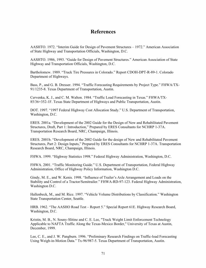
71

References

AASHTO. 1972. “Interim Guide for Design of Pavement Structures – 1972.” American Association of State Highway and Transportation Officials, Washington, D.C.

AASHTO. 1986, 1993. “Guide for Design of Pavement Structures.” American Association of State Highway and Transportation Officials, Washington, D.C.

Bartholomew. 1989. “Truck Tire Pressures in Colorado.” Report CDOH-DPT-R-89-1. Colorado Department of Highways.

Bass, P., and G. B. Dresser. 1994. “Traffic Forecasting Requirements by Project Type.” FHWA/TX-91/1235-8. Texas Department of Transportation, Austin.

Cervenka, K. J., and C. M. Walton. 1984. “Traffic Load Forecasting in Texas.” FHWA/TX-85/36+352-1F. Texas State Department of Highways and Public Transportation, Austin.

DOT. 1997. “1997 Federal Highway Cost Allocation Study.” U.S. Department of Transportation, Washington, D.C.

ERES. 2001a. “Development of the 2002 Guide for the Design of New and Rehabilitated Pavement Structures, Draft, Part 1: Introduction,” Prepared by ERES Consultants for NCHRP 1-37A. Transportation Research Board, NRC, Champaign, Illinois.

ERES. 2001b. “Development of the 2002 Guide for the design of New and Rehabilitated Pavement Structures, Part 2: Design Inputs,” Prepared by ERES Consultants for NCHRP 1-37A. Transportation Research Board, NRC, Champaign, Illinois.

FHWA. 1999. “Highway Statistics 1998.” Federal Highway Administration, Washington, D.C.

FHWA. 2001. “Traffic Monitoring Guide.” U.S. Department of Transportation, Federal Highway Administration, Office of Highway Policy Information, Washington D.C.

Gindy, M. E., and W. Kenis. 1998. “Influence of Trailer’s Axle Arrangement and Loads on the Stability and Control of a Tractor/Semitrailer.” FHWA-RD-97-123. Federal Highway Administration, Washington D.C.

Hallenbeck, M., and M. Rice. 1997. “Vehicle Volume Distributions by Classification.” Washington State Transportation Center, Seattle.

HRB. 1962. “The AASHO Road Test – Report 5.” Special Report 61E. Highway Research Board, Washington, D.C.

Kristin, M. B., N. Souny-Slitine and C. E. Lee, "Truck Weight Limit Enforcement Technology Applicable to NAFTA Traffic Along the Texas-Mexico Border," University of Texas at Austin, December, 1999.

Lee, C. E., and J. W. Pangburn. 1996. “Preliminary Research Findings on Traffic-load Forecasting Using Weigh-in-Motion Data.” Tx-96/987-5. Texas Department of Transportation, Austin.

72

Lee, C. E., and S. Nabil. 1998. “Final Research Findings on Traffic-load Forecasting Using Weigh-in-Motion Data.” Tx-98/987-7. Texas Department of Transportation, Austin.

Leidy, Joseph P., Clyde E. Lee, and Robert Harrison. 1995. “Measurement and Analysis of Traffic Loads across the Texas-Mexico Border.” Research Report 1319-1. CTR, University of Texas at Austin.

Lu, Q., and J. Harvey. 2002. “Truck Traffic Analysis Using Weigh-in-Motion (WIM) Data in California.” Pavement Research Center, University of California at Berkeley.

Middleton, D., and J. A. Crawford. 2001. “Evaluation of TxDOT’s Traffic Data Collection and Load Forecasting Process.” FHWA/TX-01/1801-1. Texas Department of Transportation, Austin.

Nelson, T. 2002. “Mn/DOT’s Office of Transportation Data and Analysis—Traffic data and MNESALS.” Traffic Forecasts and Analysis Section, MnPAVE Training, MN.

OECD. 1982. “Impact of Heavy Freight Vehicles.” RR/AP1/82.3. Organization for Economic Cooperation and Development, Paris, France.

Prozzi, J. A., and de Beer, M. 1997. “Mechanistic Determination of Equivalent Damage Factors,” Proceedings of the Eighth International Conference on Asphalt Pavements, Seattle, Washington.

Qu, T., and C. E. Lee. 1997. “Traffic-load Forecasting Using Weigh-in-Motion Data.” Tx-99/987-6. Texas Department of Transportation, Austin.

Qu, T., C. E. Lee, and L. Huang. 1998. “Traffic-load Forecasting Using Weigh-in-Motion Data.” Tx-99/987-6. Texas Department of Transportation, Austin.

TxDOT. March 1, 1993. “Standard Specifications for Construction of Highways, Streets, and Bridges.” Texas Department of Transportation, Austin.

Vlatas, A. J., and G. B. Dresser. 1991. “Traffic Load Forecasting for Pavement Design.” FHWA/TX-91/1235-1. Texas Department of Transportation, Austin.

Wang, F, R. F. Inman, R. B. Machemehl, Z. Zhang and C. M. Walton. 2000. Study of Current Truck Configurations.” Tx-00/1862-2. Texas Department of Transportation, Austin.

www.2002designguide.com. 2002. Development of 2002 Guide, NCHRP Project 1-37 A.

73

Appendix A

Effect of Axle Configuration and Load on Pavement Performance

75

y = 76.679x-1.3311

R2 = 0.976

y = 113.23x-1.5928

R2 = 0.9868

0.1

1.0

10.0

1 10 100

Load (kip)

Rel

ativ

e Li

fe SingleTandemPower (Tandem)Power (Single)

FIGURE A1: Relative life to 1 in. surface rutting, heavy pavement, Amarillo

y = 317078x-4.3775

R2 = 0.9986 y = 4E+06x-4.3857

R2 = 0.9998

0.01

0.1

1

10

1 10 100

Load (kip)

Rel

ativ

e Li

fe SingleTandemPower (Single)Power (Tandem)

FIGURE A2: Relative life to 100% cracking, heavy pavement, Amarillo

76

y = 20.847x-1.0472

R2 = 0.9616

y = 27.134x-1.0422

R2 = 0.8824

0.1

1.0

10.0

1 10 100

Load (kip)

Rel

ativ

e Li

fe SingleTandemPower (Single)Power (Tandem)

FIGURE A3: Relative life to 1 in. surface rutting, heavy pavement, Austin

y = 40492x-3.6579

R2 = 0.9863

y = 180285x-3.4738

R2 = 0.9875

0.01

0.10

1.00

10.00

10 100

Load (kip)

Rel

ativ

e Li

fe SingleTandemPower (Single)Power (Tandem)

FIGURE A4: Relative life to 100% cracking, heavy pavement, Austin

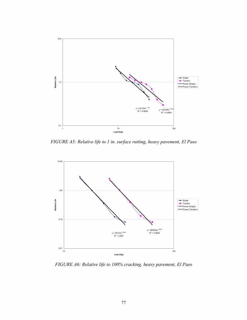
77

y = 25.232x-1.124

R2 = 0.9559y = 28.046x-1.0539

R2 = 0.9094

0.1

1.0

10.0

1 10 100

Load (kip)

Rel

ativ

e Li

fe SingleTandemPower (Single)Power (Tandem)

FIGURE A5: Relative life to 1 in. surface rutting, heavy pavement, El Paso

y = 87474x-3.9365

R2 = 0.987

y = 989200x-3.9781

R2 = 0.9826

0.01

0.10

1.00

10.00

10 100

Load (kip)

Rel

ativ

e Li

fe SingleTandemPower (Single)Power (Tandem)

FIGURE A6: Relative life to 100% cracking, heavy pavement, El Paso

78

y = 51.578x-1.2358

R2 = 0.9613

y = 48.578x-1.3109

R2 = 0.9808

0.1

1.0

10.0

1 10 100

Load (kip)

Rel

ativ

e Li

fe SingleTandemPower (Tandem)Power (Single)

FIGURE A7: Relative life to 1 in. surface rutting, heavy pavement, Houston

y = 47419x-3.7213

R2 = 0.9892

y = 261983x-3.5789

R2 = 0.9885

0.01

0.10

1.00

10.00

10 100

Load (kip)

Rel

ativ

e Li

fe SingleTandemPower (Single)Power (Tandem)

FIGURE A8: Relative life to 100% cracking, heavy pavement, Houston

79

y = 0.374x0.1399

R2 = 0.0613

y = 0.4591x0.3382

R2 = 0.507

0.1

1.0

10.0

1 10 100

Load (kip)

Rel

ativ

e Li

fe SingleTandemPower (Tandem)Power (Single)

FIGURE A9: Relative life to 0.5 in. surface rutting, light pavement, Amarillo

y = 16.97x-0.9714

R2 = 0.981

y = 32.911x-1.144

R2 = 0.995

0.1

1.0

10.0

1 10 100

Load (kip)

Rel

ativ

e Li

fe SingleTandemPower (Single)Power (Tandem)

FIGURE A10: Relative life to 100% cracking, light pavement, Amarillo

80

y = 0.5096x0.1083

R2 = 0.046

y = 0.4189x0.399

R2 = 0.5027

0.1

1.0

10.0

1 10 100

Load (kip)

Rel

ativ

e Li

fe SingleTandemPower (Tandem)Power (Single)

FIGURE A11: Relative life to 0.5 in. surface rutting, light pavement, Austin

y = 12.802x-0.8426

R2 = 0.962

y = 30.136x-1.1154

R2 = 0.9936

0.1

1.0

10.0

1 10 100

Load (kip)

Rel

ativ

e Li

fe SingleTandemPower (Single)Power (Tandem)

FIGURE A12: Relative life to 100% cracking, light pavement, Austin

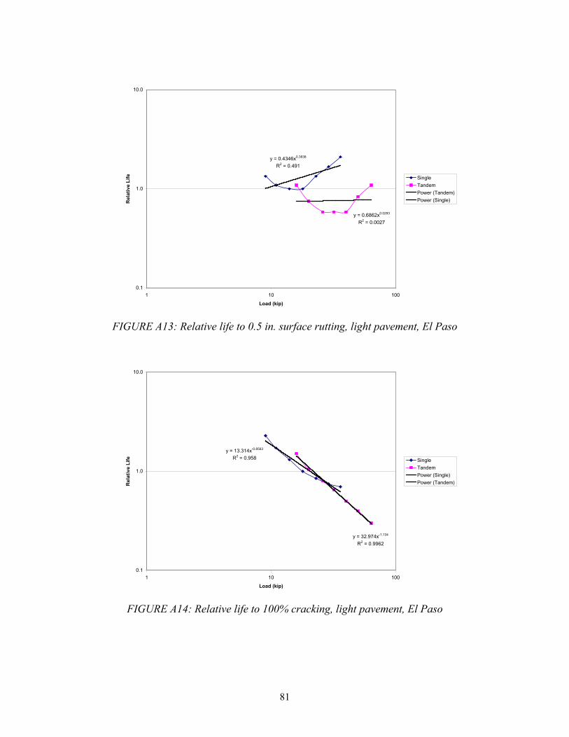
81

y = 0.6862x0.0293

R2 = 0.0027

y = 0.4346x0.3838

R2 = 0.491

0.1

1.0

10.0

1 10 100

Load (kip)

Rel

ativ

e Li

fe SingleTandemPower (Tandem)Power (Single)

FIGURE A13: Relative life to 0.5 in. surface rutting, light pavement, El Paso

y = 13.314x-0.8563

R2 = 0.958

y = 32.974x-1.134

R2 = 0.9962

0.1

1.0

10.0

1 10 100

Load (kip)

Rel

ativ

e Li

fe SingleTandemPower (Single)Power (Tandem)

FIGURE A14: Relative life to 100% cracking, light pavement, El Paso

82

y = 0.4841x0.1286

R2 = 0.0745

y = 0.4724x0.3661

R2 = 0.4111

0.1

1.0

10.0

1 10 100

Load (kip)

Rel

ativ

e Li

fe SingleTandemPower (Tandem)Power (Single)

FIGURE A15: Relative life to 0.5 in. surface rutting, light pavement, Houston

y = 10.685x-0.7812

R2 = 0.9421

y = 23.863x-1.047

R2 = 0.9909

0.1

1.0

10.0

1 10 100

Load (kip)

Rel

ativ

e Li

fe SingleTandemPower (Single)Power (Tandem)

FIGURE A16: Relative life to 100% cracking, light pavement, Houston