Evaluation of Equalization Basins as Initial Treatment for ...

Clemson UniversityTigerPrints

All Theses Theses

12-2007

Evaluation of Equalization Basins as InitialTreatment for Flue Gas Desulfurization WatersMeg IannaconeClemson University, [email protected]

Follow this and additional works at: https://tigerprints.clemson.edu/all_theses

Part of the Geology Commons

This Thesis is brought to you for free and open access by the Theses at TigerPrints. It has been accepted for inclusion in All Theses by an authorizedadministrator of TigerPrints. For more information, please contact [email protected].

Recommended CitationIannacone, Meg, "Evaluation of Equalization Basins as Initial Treatment for Flue Gas Desulfurization Waters" (2007). All Theses. 231.https://tigerprints.clemson.edu/all_theses/231

https://tigerprints.clemson.edu?utm_source=tigerprints.clemson.edu%2Fall_theses%2F231&utm_medium=PDF&utm_campaign=PDFCoverPages

https://tigerprints.clemson.edu/all_theses?utm_source=tigerprints.clemson.edu%2Fall_theses%2F231&utm_medium=PDF&utm_campaign=PDFCoverPages

https://tigerprints.clemson.edu/theses?utm_source=tigerprints.clemson.edu%2Fall_theses%2F231&utm_medium=PDF&utm_campaign=PDFCoverPages

https://tigerprints.clemson.edu/all_theses?utm_source=tigerprints.clemson.edu%2Fall_theses%2F231&utm_medium=PDF&utm_campaign=PDFCoverPages

http://network.bepress.com/hgg/discipline/156?utm_source=tigerprints.clemson.edu%2Fall_theses%2F231&utm_medium=PDF&utm_campaign=PDFCoverPages

https://tigerprints.clemson.edu/all_theses/231?utm_source=tigerprints.clemson.edu%2Fall_theses%2F231&utm_medium=PDF&utm_campaign=PDFCoverPages

mailto:[email protected]

EVALUATION OF EQUALIZATION BASINS AS

INITIAL TREATMENT FOR FLUE GAS

DESULFURIZATION WATERS

A Thesis

Presented to

the Graduate School of

Clemson University

In Partial Fulfillment

of the Requirements for the Degree

Master of Science

Hydrogeology

by

Meg M. Iannacone

December 2007

Accepted by:

Dr. James W. Castle, Committee Chair

Dr. John H. Rodgers, Jr.

Dr. C. Brannon Andersen

Dr. George M. Huddleston, III

ii

ABSTRACT

Coal-fired power plants are introducing flue gas desulfurization (FGD) scrubbers

to reduce sulfur dioxide and mercury emissions in order to meet air quality standards.

FGD scrubber systems utilize a mixture of limestone, water, and organic acids to

precipitate sulfur compounds. The resulting FGD water and associated particulates often

contain constituents of concern including chlorides, inorganic elements (Hg, As, and Se),

and sulfates that must be treated before discharge. Constructed wetland treatment

systems, consisting of an equalization basin followed by wetland reactors, present a

viable option to efficiently treat FGD waters. Equalization basins are designed to cool

and homogenize FGD water and settle particulates. Specific research objectives focused

on equalization basins are: 1) to characterize FGD particulates in terms of elemental and

mineralogical composition; 2) to determine size and settling rates of FGD particulates; 3)

to determine if Hg, As, and Se concentrations within FGD water stored in an equalization

basin change with time; and 4) to determine if toxicity of FGD water within an

equalization basin changes during a 24 hr hydraulic retention time.

The most common FGD particle type was characterized as gypsum. Other

particle types identified included fly ash and iron oxides. FGD particulates settled in an

equalization basin are interpreted to have originated during coal combustion and FGD

processes. The majority of FGD particulates were determined to be silt size, and settling

analysis shows that 95% of these particulates settled to the bottom of a typical 2.5 m deep

equalization basin within approximately 4 hrs. FGD particulates contained

concentrations of Hg, As, and Se, and as particulates settled, constituents were removed

iii

from the water column. Analysis of FGD water samples indicate that aqueous

concentrations of Hg and Se decreased in the pilot-scale equalization basins by 20 µg/L

and 200 µg/L, respectively, during a 24 hr hydraulic retention time. Data from toxicity

tests indicate that equalization basins do not decrease toxicity of FGD water to aquatic

organisms. Equalization basins are necessary for initial treatment of FGD water by

settling particulates, which may contain Hg, As, and Se. Additional treatment for these

waters occurs in the wetland reactors.

iv

DEDICATION

This thesis is dedicated to my parents for their endless support, encouragement,

and understanding throughout this endeavor.

v

ACKNOWLEDGMENTS

I would like to thank Dr. Castle for advising me during my time at Clemson and

giving me the opportunity to learn as much as I possibly could with both the

Hydrogeology Department and Dr. Rodgers’ research group. Additionally, I would like

to thank Dr. Rodgers for his guidance and expertise on toxicology subjects. I would like

to thank the other members of my committee, Dr. Andersen and Dr. Huddleston, for their

insight and individual expertise.

I would like to extend thanks to the professors at Clemson that have helped me

reach my research goals. Especially, Dr. VanDerveer for his expertise with x-ray

diffraction, Dr. Bruce for his help with particle digestions, and Dr. Chao for his help with

analytical equipment. Special thanks to the EM Lab in Pendleton as well as Dr. Mount

for guidance and help with SEM/EDS analysis.

I would like to thank the members of the lab that have not only helped me with

research and science as a whole, but have helped me grow as an individual. I especially

want to thank Laura K. and O’Niell for their true friendship.

Finally, I would like to thank Justin for his support through this chapter of my

life. His patience, understanding, and love have been priceless.

vi

TABLE OF CONTENTS

Page

TITLE PAGE....................................................................................................................i

ABSTRACT.....................................................................................................................ii

DEDICATION................................................................................................................iv

ACKNOWLEDGMENTS ...............................................................................................v

LIST OF TABLES........................................................................................................viii

LIST OF FIGURES .........................................................................................................x

CHAPTER

I. INTRODUCTION .........................................................................................1

Background and Significance ..................................................................1

Research Objectives and Methods ...........................................................8

References................................................................................................9

II. CHARACTERIZATION OF FLUE GAS

DESULFURIZATION PARTICULATES

IN EQUALIZATION BASINS .............................................................12

Abstract ..................................................................................................12

Introduction............................................................................................12

Methods..................................................................................................15

References..............................................................................................18

Discussion ..............................................................................................31

Conclusions............................................................................................38

References..............................................................................................39

III. THE ROLE OF AN EQUALIZATION BASIN

IN A CONSTRUCTED WETLAND

TREATMENT SYSTEM.......................................................................43

Abstract ..................................................................................................43

Introduction............................................................................................44

Methods..................................................................................................46

vii

Table of Contents (Continued)

Page

Results....................................................................................................54

Discussion ..............................................................................................67

Conclusions............................................................................................75

References..............................................................................................75

IV. SUMMARY AND CONCLUSIONS ..........................................................80

Introduction............................................................................................80

Characterization of flue gas desulfurization

particulates in equalization basins ...................................................82

The role of an equalization basin in a constructed

wetland treatment system.................................................................83

Conclusions............................................................................................84

References..............................................................................................84

APPENDICES ...............................................................................................................86

A: Standard Operating Procedures for Characterizing

FGD Particulates....................................................................................87

B: Standard Operating Procedures to Determine

Treatment in an Equalization Basin.....................................................101

viii

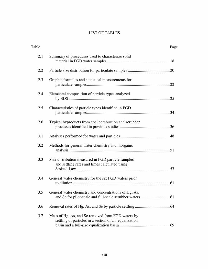
LIST OF TABLES

Table Page

2.1 Summary of procedures used to characterize solid

material in FGD water samples..............................................................18

2.2 Particle size distribution for particulate samples .........................................20

2.3 Graphic formulas and statistical measurements for

particulate samples.................................................................................22

2.4 Elemental composition of particle types analyzed

by EDS...................................................................................................25

2.5 Characteristics of particle types identified in FGD

particulate samples.................................................................................34

2.6 Typical byproducts from coal combustion and scrubber

processes identified in previous studies.................................................36

3.1 Analyses performed for water and particles ................................................48

3.2 Methods for general water chemistry and inorganic

analysis...................................................................................................51

3.3 Size distribution measured in FGD particle samples

and settling rates and times calculated using

Stokes’ Law ...........................................................................................57

3.4 General water chemistry for the six FGD waters prior

to dilution...............................................................................................61

3.5 General water chemistry and concentrations of Hg, As,

and Se for pilot-scale and full-scale scrubber waters.............................61

3.6 Removal rates of Hg, As, and Se by particle settling ..................................64

3.7 Mass of Hg, As, and Se removed from FGD waters by

settling of particles in a section of an equalization

basin and a full-size equalization basin .................................................69

ix

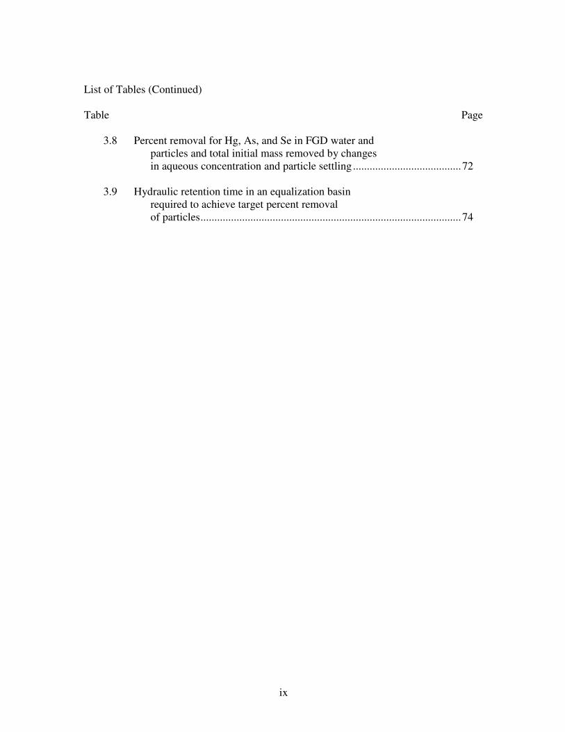
List of Tables (Continued)

Table Page

3.8 Percent removal for Hg, As, and Se in FGD water and

particles and total initial mass removed by changes

in aqueous concentration and particle settling .......................................72

3.9 Hydraulic retention time in an equalization basin

required to achieve target percent removal

of particles..............................................................................................74

x

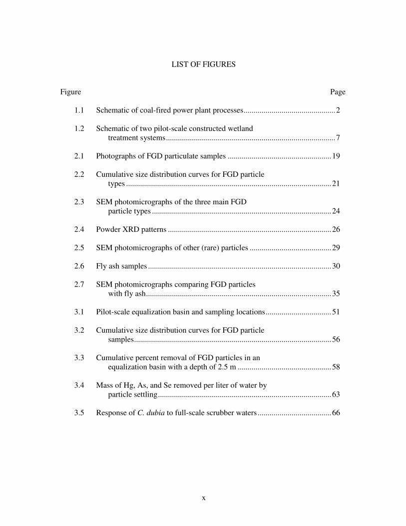
LIST OF FIGURES

Figure Page

1.1 Schematic of coal-fired power plant processes..............................................2

1.2 Schematic of two pilot-scale constructed wetland

treatment systems.....................................................................................7

2.1 Photographs of FGD particulate samples ....................................................19

2.2 Cumulative size distribution curves for FGD particle

types .......................................................................................................21

2.3 SEM photomicrographs of the three main FGD

particle types ..........................................................................................24

2.4 Powder XRD patterns ..................................................................................26

2.5 SEM photomicrographs of other (rare) particles .........................................29

2.6 Fly ash samples ............................................................................................30

2.7 SEM photomicrographs comparing FGD particles

with fly ash.............................................................................................35

3.1 Pilot-scale equalization basin and sampling locations.................................51

3.2 Cumulative size distribution curves for FGD particle

samples...................................................................................................56

3.3 Cumulative percent removal of FGD particles in an

equalization basin with a depth of 2.5 m ...............................................58

3.4 Mass of Hg, As, and Se removed per liter of water by

particle settling.......................................................................................63

3.5 Response of C. dubia to full-scale scrubber waters .....................................66

1

CHAPTER I

INTRODUCTION

Background and Significance

Coal combustion accounts for about half of the energy produced currently in the

United States (EIA, 2005). In 2004, coal burned by electrical power plants reached 1,016

million short tons (EIA, 2005), which accounts for 92% of the total coal used in the

United States. Coal varies in composition of both organic and inorganic compounds.

Organic compounds in coal occur from the remains of plant material and include C, H, O,

N, and S as major elements (Malvadkar et al., 2004). Over 120 inorganic compounds can

be found within different types of coal (Schweinfurth, 2005). Some of the primary

inorganic elements in coal include aluminum, silicon, calcium, magnesium, sodium, and

sulfur with secondary elements including zinc, cadmium, manganese, arsenic,

molybdenum, and iron (Malvadkar et al., 2004).

Coal used for electrical power is crushed, pulverized, and blown into a

combustion chamber where it immediately ignites (Kalyoncu, 1999) (Figure 1.1). The

specific composition of coal determines the way in which the coal burns. On the basis of

several parameters, including fixed carbon, volatile matter, and moisture content, coal is

ranked into four different classes: anthracite, bituminous, subbituminous, and lignite

(Malvadkar et al., 2004). Quality of coals that are used in electrical power plants is

determined by observing the environmental issues that surround the characteristics of

burning the coal. These include sulfur dioxide emissions, hazardous air pollutants,

carbon dioxide emissions, and ash properties (Schweinfurth, 2005).

2

Figure 1.1: Schematic of coal-fired power plant processes.

As coal is burned, uncombusted material forms fly ash and some elements, such

as mercury and selenium, volatilize and become part of flue gas (Schweinfurth, 2005).

Flue gas contains high levels of sulfur dioxide (SO2), nitrogen oxide (NOx), particulates,

and carbon dioxide (CO2) (USEPA, 2005). Traditionally, flue gas has been emitted

through smoke stacks. Amendments made to the Clean Air Act in 1977 included the

reduction of power plant emissions for new coal-fired power plants. In 2003, the

“Interstate Air Quality Rule” was incorporated by the United States Environmental

Protection Agency (USEPA), which regulates sulfur dioxide and nitrous oxide emissions

for existing and new power plants (Smith, 2004). For the first time in 2005, the USEPA

added the “Clean Air Mercury Rule” to the pre-existing Clean Air Act to regulate

mercury emissions from coal-fired powered plants (EPA, 2005). Power plants under the

COAL

(containing organics

and inorganics)

BURNER (coal is crushed

and ignited)

FLUE GAS

(containing SO2, NOX,

and particulates)

SLURRY

(limestone, water, and

organic acids added)

SCRUBBER

(flue gas desulfurization

[FGD])

DEWATERING

OF PRODUCT

GYPSUM

(used for the production

of wallboard)

WATER

(high concentrations

of Cl, Hg, As, Se)

3

jurisdiction of the USEPA must abide by these new emission reductions by the year

2010.

To comply with these laws, coal fired power plants are incorporating flue gas

desulfurization (FGD) scrubbing processes to remove sulfur dioxide from flue gas.

Several different scrubber options are available for coal-fired power plants. In the United

States the most popular system is the calcium (limestone)-based wet scrubber (Kalyoncu,

1999). Wet limestone desulfurization systems can remove 95% of sulfur dioxide from

flue gas (Termuehlen and Emsperger, 2003). Through this process, a mixture of

limestone (CaCO3), water, and organic acid are sprayed down onto the flue gas.

Limestone reacts with sulfur dioxide to form calcium sulfite, which when further

oxidized forms calcium sulfate (CaSO4) (Mierzejewski, 1991). Organic acids, such as

dibasic acid, are used to improve the sorption properties of the limestone (Karatepe,

2000). Reactions that remove sulfur dioxide from flue gas also have the ability to remove

some of the harmful vapor pollutants including mercury and selenium. The degree to

which these constituents are removed depends on their initial concentrations, the type of

coal burned, and the type of scrubber. Although the FGD process removes constituents

from the vapor form, it condenses byproducts that may enter the environment through

new routes (Hatanpää et al., 1997), such as water discharge.

Sludge produced from the FGD process is dewatered using belt presses, vacuum

filtration, or centrifugation. The resulting product is a solid material composed of

gypsum used in the production of wallboard. By 1999, production of wallboard using

synthetic gypsum from FGD sludge increased greatly from previous years to

4

approximately 4 million tons a year (Kalyoncu, 1999), and continues to increase with the

construction of FGD scrubbers for existing and new coal-fired power plants.

In the dewatering process, the water and any suspended particulates not removed

may not meet National Pollutant Discharge Elimination System (NPDES) permits for

discharge. The degree of treatment required for FGD water continues to increase as

discharge limits continue to decrease (Mierzejewski, 1991). Composition of this water

varies among scrubber units and power plants because of differences in the original coal

being burned and the limestone and water used during the flue gas scrubbing process.

Constituents of concern within FGD water include, but are not limited to, inorganic

elements (e.g. Hg, As, Se), chlorides, sulfates, and total suspended solids (TSS).

Mercury, arsenic, and selenium are the major constituents of concern based on toxicity of

the element, high concentrations of these elements measured in the water, and discharge

permits.

Concentrations of major constituents of concern (Hg, As, and Se) may vary orders

of magnitude depending on type of coal burned, scrubber unit and materials, and

composition of any other water used within the system. Mercury, an inorganic element

that occurs naturally in the environment at low concentrations, has increased in the

atmosphere and surface waters due to coal-fired power plant emissions. Mercury occurs

in several forms including elemental, mercurous [Hg(I)], mercuric [Hg(II)], and

methylmercury (MADEP, 1996). The specific forms of mercury within flue gas and

FGD water are still being studied. Although selenium occurs naturally in the

environment and is a micronutrient for organisms, excessive amounts of selenium elicit

5

toxic effects (ATSDR, 2003). There are four major forms of selenium including

elemental, selenate [Se(VI)], selenite [Se(IV)], and selenide [Se(-II)]. Arsenic is found

naturally in the environment, and its concentration has increased due to anthropogenic

processes (ATSDR, 2005). There are three main forms of arsenic including elemental,

arsenite [As(III)], and arsenate [As(V)]. The fate of mercury, arsenic, and selenium are

greatly influenced by pH, Eh (redox potential), and other chemical species present within

the system.

Large volumes of water from FGD scrubbers are produced daily. In a single

North Carolina power plant 0.5 – 1.75 million gallons per day of water are produced

(Mooney et al., 2006). Because FGD water contains toxic constituents, there is a

tremendous need to treat the water efficiently. The treatment options available must also

be cost effective and economically feasible to efficiently remove constituents of concern.

Specifically designed constructed wetland treatment systems (CWTS) can provide

effective treatment to several types of wastewater and are being utilized by industry to

meet water quality discharge limits. Some of the more common uses for CWTS have

been to treat municipal wastewater, acid mine drainage, pulp mill effluent, refinery

effluent, agricultural wastes, urban runoff, and landfill leachate (Watson et al., 1989).

CWTS are designed to target specific constituents, such as organic and inorganic

elements and compounds, for maximum removal through transfers and transformations.

Specific transfers and transformations include, but are not limited to, retention,

sequestration, precipitation, biotransformation (microbial activity), and abiotic

transformations (oxidation, hydrolysis, and photolysis) (Rodgers, 2004). Constructed

6

wetland treatment systems are largely self maintaining and a cost-effective method to

treat constituents of concern in different FGD waters. From experiments with FGD water

and pilot-scale constructed wetland treatment systems, targeted constituents have been

effectively removed and specific discharge limits have been met.

CWTS generally contain an equalization basin followed by a series of reactors

containing vegetation and hydrosoil selected to promote specific transfers or

transformations of constituents of concern. At Clemson University microcosm

constructed wetland treatment systems were configured to evaluate the removal of

mercury, arsenic, and selenium from FGD waters. Treatment systems consisted of four

separate 70-gallon wetland reactors (Rubbermaid® Utility Tanks) (Figure 1.2). Prior to

entering the reactors, FGD water was retained in a 1,000-gal polypropylene equalization

basin. This water was pumped from the equalization basin to the reactors using piston

pumps (FMI®

) calibrated to a specific flow rate to maintain a predetermined hydraulic

retention time (HRT). The water was carried from one reactor to the next by gravity

using PVC piping. The first and second reactors of each treatment system contained

approximately 30 cm thickness of hydrosoil amended with organic matter to promote

reducing conditions within the reactors. These reactors were planted with

Schoenoplectus californicus, giant bulrush. The third wetland reactor featured a rock

cascade constructed of medium-sized granite rocks to oxygenate the water as it entered

the reactor. Both the third and fourth reactors contained approximately 30 cm of

hydrosoil and were planted with Typha agustifolia, cattails, to aid in the oxidation of the

hydrosoil.

7

Pumps

Flow

12

Reactor 1 Reactor 2

Rock Cascade

and Reactor 3

Reactor 4

Equalization

Basin

Figure 1.2: Schematic of two pilot-scale constructed wetland treatment systems.

Reactors 1 and 2 are planted with S. Californicus and Reactors 3 and 4 are planted with

T. agustifolia.

Full-scale equalization basins are constructed retention pools used to store water

and as the primary step in many water treatment systems. Equalization basins have

retained waters including sewage, ash sluice, surface mine, and surface runoff waters

(Cherry et al., 1984; Greenburg, 1986; Somes et al., 2000). The selection for the design

of equalization basins is based on many factors including the size of the power plant,

local regulatory policy, site conditions, engineer’s judgment and experience, and

economics (WEF and ASCE, 1992).

Equalization basins of constructed wetland treatment systems have not been

adequately studied. To date, there has been no treatment (transfers or transformations of

constituents) for FGD water attributed to the equalization basin. Major purposes of

equalization basins include cooling and homogenizing FGD water and settling

particulates before this water enters the reactors of the system. FGD water entering an

equalization basin is typically 40°C with up to 1,000 mg/L particulates (Mooney, 2006,

written communication). The hydraulic retention time for FGD water in an equalization

8

basin is generally 24 hours. FGD water is cooled to avoid exposing the macrophytes

planted in the CWTS reactors to high temperatures. The settling of particulates in the

equalization basin increases the longevity of the CWTS by keeping unwanted particles

out of the wetland reactors.

Research Objectives and Methods

The specific objectives of this research include:

• Characterize FGD particulates (elements and minerals) from

different burned coals that settled in an equalization basin.

• Measure particle size distribution of FGD particulate samples.

• Determine if FGD particles settle within an equalization basin and

what the settling rates of these particles are within FGD water

samples.

• Determine if Hg, As, and Se concentrations decrease over time

within FGD water stored in an equalization basin.

• Determine if the toxicity of FGD water changes within an

equalization basin during a hydraulic retention time of 24 hours.

The second chapter of this thesis focuses on characterizing FGD particulates

(elemental and mineralogical analysis and particle size) that settle in an equalization

basin. Four FGD particulate samples obtained from a pilot-scale scrubber were analyzed.

To determine the minerals and elements that comprise FGD particulates from different

burned coals, x-ray diffraction and scanning electron microscopy (SEM) equipped with

electron dispersive spectroscopy (EDS) were utilized. The pipette method (Folk, 1980)

was used to determine particle size distribution of FGD particulates.

9

The third chapter of this thesis focuses on the role of an equalization basin in

treatment of FGD water. Size distribution of the FGD particulates was used along with

settling velocity of particulates (Stokes’ Law) to determine the time period for

particulates to settle in a typical equalization basin with a certain depth. To determine the

removal of targeted constituents (Hg, As, and Se) in equalization basins, two pilot-scale

equalization basins were utilized. Chemical analyses of six FGD waters were determined

for initial and final samples, which simulated inflow and outflow of an equalization

basin. Particulates suspended in two of the FGD water samples were digested to

determine the concentrations of Hg, As, and Se associated with the particulates. Toxicity

of initial and final samples for two FGD waters was measured using a microcrustacean,

Ceriodaphnia dubia.

Understanding the processes that occur in a constructed wetland treatment system

is important for removal of specified constituents for different types of water. Each

specific part of a CWTS plays an important role in the removal of constituents of concern

and has been designed accordingly for performance. This research will provide further

understanding of the role of the equalization basin as a component of a constructed

wetland treatment system.

References

Agency for Toxic Substances and Disease Registry (ATSDR), 2003, ToxFAQsTM

for

Selenium. US Department of Health and Human Services.

http://www.atsdr.cdc.gov/tfacts92.html accessed: 12/05/05

Agency for Toxic Substances and Disease Registry (ATSDR), 2005, ToxFAQsTM

for

Arsenic. US Department of Health and Human Services.

http://www.atsdr.cdc.gov/tfacts2.html accessed 12/05/05

10

Cherry, D.S., Guthrie, R.K., Davis, E.M., and Harvey, R.S., 1984, Coal ash basin effects

(particles, metals, acidic pH) upon aquatic biota: An eight-year evaluation:

Water Resources Bulletin, v. 20, p. 535-544.

EIA, Energy Information Association, 2005, Annual Coal Report 2004, 74 p.

Folk, R.L., 1980, Petrology of Sedimentary Rocks: Austin, Hemphill Publishing

Company, 184 p.

Greenburg, J.A., 1986, A rational approach to the design operation and maintenance of

sediment basins [M.S. thesis]: Clemson, Clemson University, 170 p.

Hatanpää, E., Kajander, K., Laitinen, T., Piepponen, S., and Revitzer, H., 1997, A

study of trace element behavior in two modern coal-fired power plants: I.

Development and optimization of trace element analysis using reference

materials: Fuel Processing Technology, v. 51, p. 205-217.

Hurlbut, C.S., 1971, Dana’s Manual of Mineralogy, Eighteenth Edition: New York,

JohnWiley & Sons Inc., 579 p.

Kalyoncu, R.S., 1999, Coal Combustion Production. U.S. Geological Survey

MineralsYearbook-1999, p. 19.1-19.4.

Karatepe, N., 2000, A Comparison of Flue Gas Desulfurization Processes: Energy

Sources, v. 22, p. 197-206.

MADEP, Massachusetts Department of Environmental Protection, 1996, Mercury:

Forms, Fate & Effects. http://www.mass.gov/dep/toxics/stypes/hgch2.htm

accessed: 10/14/05

Malvadkar, S.B., Forbes, S., D., McGurl, G.V., 2004, Formation of Coal Resources:

Encyclopedia of Energy, v. 1, p. 529-550.

Mierzejewski, M.K., 1991, The Elimination of Pollutants from FGD Wastewaters,

The 1991 SO2 Control Symposium. Washington D.C., 20 p.

Mooney, D., Rodgers, J.H. Jr., Murray-Gulde, C. and Huddleston, G.M. III, 2006,

Constructed Wetlands Treatment Systems for FGD Waters: Full Scale, 14th

Annual David S. Snipes/Clemson Hydrogeology Symposium Abstracts with

Programs, p. 18.

Rodgers, J.H., Jr., 2004, What Are Constructed Wetlands? Constructed Wetlands for

Water Quality Improvement: A Short Course presented by Clemson University

and ENTRIX, Inc. Clemson, SC.

11

Schweinfurth, S.P., 2005, Coal-A Complex Natural Resource: USGS

http://pubs.usgs.gov/circ/c1143/html/text.html accessed: 11/20/05

Smith, D., 2004, The Emissions Squeeze: Power Engineering, v. 108, p. 26-28.

Somes, N.L.G., Fabian, J., Wong, T.H.F., 2000, Tracking pollutant detention in

constructed stormwater wetlands: Urban Water, v. 2, p. 29-37.

Termuehlen, H. and Emsperger, W., 2003, Clean and Efficient Coal-Fired Power Plants:

New York, ASME Press, 143p.

USEPA, 2005, Clean Energy: Electricity from Coal. United States Environmental

Protection Agency http://www.epa.gov/cleanenergy/coal.htm accessed:

12/05/05

USEPA, 2005, Mercury: Laws and Regulations. United States Environmental

Protection Agency http://www.epa.gov/mercury/regs.htm accessed:

12/05/05

Watson, J.T., Reed, S.C., Kadlec, R.H., Knight, R.L., and Whitehouse, A.E., 1989,

Performance expectations and loading rates for constructed wetlands, in Hammer,

D.A., ed., Constructed wetlands for wastewater treatment municipal, industrial

and agricultural, Lewis Publishers Inc., Michigan, p. 319-351.

Water Environment Federation (WEF) and American Society of Civil Engineers (ASCE),

1992, Design of Municipal Wastewater Treatment Plants Volume I: Chapters 1-

12, 829.

12

CHAPTER II

CHARACTERIZATION OF FLUE GAS DESULFURIZATION

PARTICULATES IN EQUALIZATION BASINS

Abstract

Particulates that settle from flue gas desulfurization (FGD) water in an

equalization basin of a constructed wetland treatment system were characterized

physically and chemically. Powder x-ray diffraction and scanning electron microscopy

with electron dispersive spectroscopy were used to identify mineralogy and elemental

composition of the particulates. Settling analysis based on Stokes’ Law was performed to

determine particle size. The most common particle type was gypsum (CaSO4·2H2O)

comprising approximately 95% of the samples. A second particle type was interpreted as

fly ash and comprises up to 5% of the samples. The fly ash particles contained carbon

and metals including Al, Fe, Mg, and Ti. Minor particles containing Fe, Al, K, and Si

were interpreted as oxides formed in the coal combustion chamber. FGD particulates

contain a mixture of solids representing combustion and wet scrubbing processes at coal-

fired power plants.

Introduction

New laws implemented by the United States Environmental Protection Agency

(USEPA) require coal-fired power plants to reduce gaseous emissions of sulfur dioxide

and mercury vapors (Schweinfurth, 2005). To comply with these laws, flue gas

13

desulfurization (FGD) scrubbers are being added to existing power plants. The most

common system used in the United States is the calcium (limestone)-based wet scrubber

(Kalyoncu, 1999), which can remove 95% of sulfur dioxide from flue gas (Termuehlen

and Emsperger, 2003). In the FGD process, a slurry of water, limestone (CaCO3), and

organic acids mixes with the sulfur dioxide and forms calcium sulfite, which when

further oxidized, forms calcium sulfate. This slurry is then dewatered, producing large

amounts of water and gypsum, a byproduct used in production of wallboard (Kovacs and

Molnar, 2003). In 2005, domestic coal-fired power plants in the United States produced

11.95 million metric tons of gypsum through the FGD process (American Coal Ash

Association, 2006), with estimates showing that production will increase (Founie, 2004).

Solid product not removed during the dewatering process remains suspended within FGD

water.

Composition of the FGD water and associated particulates depends on

composition of the burned coal, scrubbing materials such as limestone, and slurry water

used in the FGD process (Mierzejewski, 1991). FGD water may require treatment prior

to discharging to the environment in order to meet limits set by the USEPA for

concentrations of inorganic and organic constituents. Mercury, arsenic, and selenium

concentrations are of the greatest concern within FGD water.

Our investigation focuses on FGD particulates in equalization basins of

constructed wetland treatment systems (CWTS). CWTS are being built at coal-fired

power plants to treat FGD waters for discharge or reuse. CWTS are proving to be a

viable option for this purpose. These systems target a wide range of constituents in many

14

types of wastewaters (Knight et al., 1999; Gillespie et al., 2000; Murray-Gulde et al.,

2003a; 2003b) and can reduce concentrations of constituents that do not meet National

Pollutant Discharge Elimination System (NPDES) limits. Pilot-scale treatment systems

are used to monitor treatment and then predict performance of future full-scale CWTS.

The basic design of CWTS used for treatment of FGD water includes an equalization

basin followed by reactors containing vegetation and hydrosoil selected to promote

specific transfers and transformations of constituents of concern.

An equalization basin is a constructed retention pool that allows water to cool and

homogenize and particulates to settle. At thermo-electric power plants, FGD water enters

the equalization basin at a temperature of approximately 40°C and may contain

particulate concentrations of 1,000 mg/L (Mierzejewski, 1991; Doug Mooney, 2006,

written communication). Equalization basins used for FGD water are usually designed to

store water for one day and cool the water to 35°C (McCarthey et al., 2005).

Equalization basin design parameters include daily water volume produced by the power

plant, settling rate of particulates, and geographic location of the power plant.

Byproducts of coal combustion and flue gas desulfurization include fly ash,

bottom ash, boiler slag, and FGD sludge. Many past studies (Khanra et al., 1998;

Sulovsky, 2002; Gieré et al., 2003; and Pires and Qeurol, 2004) have focused on

characterization of fly ash, which is uncombusted material produced after coal powders

burn at temperatures between 1300 and 1500°C (Ma et al., 1999). However, very few

studies (Laperche and Bigham, 2002; Kovacs and Molnar, 2003; and Bigham et al.,

2005) have focused on FGD particulates and sludge.

15

The purpose of this investigation was to characterize particulates that settle within

an equalization basin of a constructed wetland system used to treat FGD water. The

objectives were: 1) to determine physical properties and elemental and mineralogical

compositions of FGD particulate samples; and 2) to measure particle size distribution of

the samples. Analytical results were compared with published descriptions of coal

combustion byproducts from thermoelectric power plants. Origin of particulates was

interpreted from characterizing minerals and elements present in the samples. Identifying

types of particulates settling from FGD water in an equalization basin is necessary for

determining optimal reuse and disposal procedures once the maximum capacity of the

basin is reached. This analysis may be useful for the design of future equalization basins

of CWTS.

Methods

Particles were collected from four FGD water samples (numbered 1 to 4), each of

which was obtained from a pilot-scale wet scrubber located at a coal-fired power plant in

North Carolina. Each water represented combustion of a different low-sulfur eastern

bituminous coal. The FGD waters were transported to Clemson University for treatment

in a pilot-scale CWTS. In addition, a fly ash sample collected from a coal-fired power

plant in North Carolina was analyzed. The fly ash was the product of burning a low-

sulfur bituminous coal.

Color, shape, crystal form, size, and surface texture of the FGD particulates were

observed using a stereographic binocular microscope. Color provided a useful

discriminator for separating particles. Black particles were separated into magnetic and

16

non-magnetic fractions using a hand magnet. Following methodology of Folk (1980),

particle size distribution was determined for FGD particulates collected from two of the

four waters (Table 2.1). Sample size was too small to determine particle size distribution

for the other two samples. Approximately 15-20 g of samples was needed to perform the

analysis. Sand size particles were separated using a 62 micron sieve, dried, and weighed.

The finer fraction (<62 µm) was suspended in a 1,000 mL graduated cylinder filled with

distilled water. Following methodology of Folk (1980), a pipette was used to withdraw

samples from the graduated cylinder at specific time intervals. The samples were then

dried at 100ºC for 24 hours and weighed. The times and withdrawal depths for particles

were calculated using Equation 1:

Equation 2.1

where T is time (min), Depth is the sampling depth (cm), A is a constant based on

viscosity of water, gravity, and density of the particles, and d is the particle diameter

(mm). An A value for a particle density of 2.32 gm/cc (gypsum) was extrapolated using

known A values (Folk, 1980; Gee and Bauder, 1986) for particle densities 2.4, 2.65, 3.0,

and 3.35 gm/cc. The A value used in this experiment was 3.00, which was based on a

water temperature of 22ºC. Cumulative particle size distribution curves were constructed

from weights of the size fractions. Statistical parameters including graphic mean,

median, mode, inclusive graphic standard deviation and skewness, and graphic kurtosis

were calculated using values from the distribution curves.

2**1500 dA

DepthT =

17

An Hitachi 3400 Scanning Electron Microscope (SEM) was used to characterize

features of particles and identify any particle types not recognized using a binocular

microscope. Samples for SEM analysis were prepared by adhering dried particles to

carbon tape-covered stubs (specimen mounts). Each particle type was mounted on a

separate stub. Elemental composition of individual particles was determined with

elemental dispersive spectroscopy (EDS) using an Oxford Inca 400 EDS with the Oxford

Instrument software package INCA.

Mineral composition of particles was determined by powder x-ray diffraction

(XRD) using a Scintag 2000 diffractometer and a Rigaku Miniflex diffractometer.

Samples were powdered using a porcelain mortar and pestle. The XRD data were

collected from 2-60° 2θ at a step scan rate of 0.04 deg/min using a CuKα x-ray source.

In addition to samples listed in Table 2.1, sand size particles separated from FGD

samples 1, 3, and 4, and silt and clay size particles separated from FGD samples 1 and 2

were analyzed by XRD. A mixture of sand size black and white particles was analyzed

separately from the other particle samples. Splits of FGD samples 3 and 4 were exposed

to dilute acetic acid for removal of carbonate minerals according to United States

Geological Survey (USGS) methods (Poppe et al., 2001) and then analyzed by XRD.

Diffraction peaks were identified using Scintag-DSMNT and Jade 5 software and by

matching d-spacings to published values.

18

Table 2.1: Summary of procedures used to characterize solid material in FGD water

samples. The methods include visual observation, particle size distribution (PSD), x-ray

diffraction (XRD), and scanning electron microscopy with energy dispersive

spectroscopy (SEM/EDS).

1from all FGD samples 2from FGD Samples 4 3from FGD Samples 1, 2, 3

Results

Bulk FGD Particulates

FGD samples 1 through 4 ranged in color from light brown to dark-grayish

brown. Wet FGD samples were muddy in consistency due to a high content of silt and

clay size material. After drying the particulate samples, it was observed that three main

types of particles were present based on color: white, orange, and black (Figure 2.1).

Particle size distribution was unimodal in both samples analyzed (Tables 2.2;

Figure 2.2), with each sample consisting predominantly of silt-size particles (2-62.5 µm).

The graphic mean size of FGD sample 3 is 5.3 φ with an inclusive graphic standard

deviation of 0.34 φ, indicating very well sorted medium silt (Table 2.3). FGD sample 4

particles have a graphic mean of 4.7 φ with an inclusive graphic standard deviation of

Sample

Procedures

Visual PSD XRD SEM/EDS

FGD Sample 1 X X X

FGD Sample 2 X X X

FGD Sample 3 X X X X

FGD Sample 4 X X X X

White Particles1 X X X

Black Particles2 X X X

Orange Particles3 X X

Other (rare) Particles X

Fly Ash Particles X X X X

19

0.29 φ, which corresponds to very well sorted coarse silt. The inclusive graphic

skewness for both samples was determined to be near symmetrical, indicating that the

size distribution curve is approximately symmetrical about the mean. The graphic

kurtosis determined by the size distribution curve indicates that FGD sample 3 is very

leptokurtic and FGD sample 4 is leptokurtic. Therefore, particle sizes near the mean are

better sorted than particle sizes further from the mean. The statistical parameters indicate

that the FGD particulate samples have a narrow range in size.

Figure 2.1: Photographs of FGD particulate samples. (A) Sand size white particles and

black particles from FGD sample 4. (B) White particles and an orange aggregate

(outlined) within the >62.5 µm (sand size) fraction of FGD sample 1.

A

0.4 mm

B

0.6 mm

20

Table 2.2: Particle size distribution for FGD samples 3 and 4, phi (φ) = -log2 (diameter in

mm); grain size name based on Wentworth (1922). Cumulative values were interpolated

from the grain size curves (Figure 2.2).

Diameter Phi Scale Wentworth Cumulative %

(mm) (φ) Size Class FGD sample 3 FGD sample 4

0.0625 4 v. fine sand 0.65 2.27

0.053 4.25 coarse silt 3.05 6.90

0.044 4.5 coarse silt 5.10 18.5

0.037 4.75 coarse silt 7.41 52.2

0.031 5 coarse silt 14.5 78.1

0.022 5.5 medium silt 87.1 96.6

0.016 6 medium silt 96.5 97.8

0.011 6.5 medium silt 98.0 99.1

0.0078 7 fine silt 98.5 99.3

0.0055 7.5 fine silt 99.0 99.5

0.0039 8 v. fine silt 99.0 99.8

0.0028 8.5 v. fine silt 99.1 99.8

0.002 9 clay 99.1 99.9

21

Figure 2.2: Cumulative size distribution curves. (A) FGD sample 3 (B) FGD sample 4

A

7 9

0

20

40

60

80

100

4 5 6 7 8

Cum

ula

tive

%

B

Grain Diameter (φ) 4 5 6 7 8 9

0

20

40

60

80

100

4 5 6 7 8 9

0

20

40

60

80

100

Grain Diameter (φ)

Cu

mu

lati

ve

%

22

Table 2.3: Graphic formulas and statistical values (Folk, 1980) for FGD samples 3 and 4.

All values (φ16, φ50, φ84, etc.) in the equations are determined from the cumulative curves

(Figure 2.2), where φx corresponds to the phi value at x cumulative percent. IG =

Inclusive graphic, NS = Near symmetrical

Value

Name Equation FGD sample 3 FGD sample 4

Graphic

(φ16 + φ50 + φ84) 5.3 φ 4.7 φ

Mean

Mz =

. 3 medium silt coarse silt

Median Md = φ50 5.3 φ 4.7 φ

Most frequently-occurring Mode Mo =

particle diameter 5.2 φ 4.8 φ

IG Standard φ84 - φ16 + φ95 – φ5 0.34 φ 0.29 φ

Deviation σ1 =

4 6.6 v. well sorted v. well sorted

IG φ84 + φ16 - 2φ50 + Φ95 + φ5 - 2φ50 -0.09 0.06

Skewness Sk1 =

2(φ84 - φ16) (φ95 – φ5) NS NS

(φ95 - φ5) 2.8 1.2 Graphic

Kurtosis KG =

2.44(φ75 - φ25) v. leptokurtic leptokurtic

FGD Particle Types

Translucent White Particles

White particles were the most common (~95% based on visual observation)

particle type represented in FGD samples 1 through 4. The size of these particles ranged

from clay to sand. The sand-size particles were mostly vitreous and translucent. Many of

the white particles were crystalline with a rhombohedral shape. The surfaces of the

rhombehedral particles appeared smooth with rare divots (Figure 2.3A). Shape of non-

rhombehedral white particles (Figure 2.3B) were rounded, and sphericity was high based

on the classification of Powers (1953) cited by Folk (1980). Small rows of indentations

were present across the surface of the non-rhombehedral white particles (Figure 2.3B).

23

SEM examination revealed that small spheres (<1 µm diameter) were attached to the

white particles (Figure 2.3B).

Based on elemental analysis by EDS, individual white particles contained oxygen,

carbon, calcium, and sulfur with trace amounts (~1%) of silicon and aluminum (Table

2.4). A dark, circular indentation was observed in one white particle. EDS analysis of

the indentation detected fluorine (5%), aluminum (~1%), and silicon (~1%) in addition to

carbon, oxygen, calcium, and sulfur.

Calcium sulfate hydrate (gypsum) was identified by XRD as the predominant

mineral in FGD samples 1 through 4, the sand size particles collected from FGD samples

1, 3, and 4, and the silt and clay size particles separated from FGD samples 1 and 2

(Figure 2.4A). Samples treated with acetic acid for removal of carbonates did not show a

difference in XRD pattern between pre-treatment and post-treatment, indicating that

carbonate minerals are not present within FGD samples 3 and 4 or do not represent a

large enough fraction to be identified using XRD.

The white particles in the FGD samples were identified as gypsum (CaSO4·2H2O)

based on crystal shape, EDS analysis, and XRD. The EDS data indicate that the molar

ratio between sulfur and calcium is 1:1 and the molar ratio between calcium and oxygen

is 1:6. The sulfur to calcium ratio is consistent with the empirical formula for calcium

sulfate. However, the empirical formula for calcium sulfate requires only four moles of

oxygen per mole of calcium instead of the observed six. The excess oxygen is accounted

for by the presence of water in hydrated calcium sulfate (gypsum).

24

Figure 2.3: SEM photomicrographs of the three main FGD particle types. (A) White

particle with well defined rhombehedral crystal form; small divots are present on the

grain surface. (B) White particle with round shape and rough surface; small spheres are

attached to upper portion of the particle. (C) Black particle with pitted surface. (D) Black

particle with partially hollow interior. (E) Orange aggregate.

20 µm 25 µm

45 µm 30 µm

C D

125 µm

E

A B

25

Table 2.4: Elemental composition of particle types analyzed by EDS. Mean percent (and

range) are listed based on 6 white particles (18 points of elemental analysis), 7 orange

particles (23 points of elemental analysis), and 8 black particles (5 non-magnetic, 3

magnetic; 17 points of elemental analysis). ND = Not Detected

Orange Non-magnetic Magnetic

White Particles Particles Black Particles Black Particles

Mean (Range) Mean (Range) Mean (Range) Mean (Range)

C 14 (3.7 - 30) 20 (9.5 - 45) 70 (54 - 82) 27 (4.0 – 70)

O 48 (31 - 57) 42 (19 – 54) 17 (12 - 24) 37 (19 - 54)

Al 0.10 (0 - 0.72) 3.7 (0.35 – 12) 1.7 (0 - 3.5) 3.8 (0.85 - 7.7)

Si 0.16 (0 - 0.98) 17 (0.63 – 30) 4.0 (0.91 - 8.3) 13 (1.3 – 22)

S 15 (0.91 - 22) 0.40 (0 - 1.2) 2.3 (0.81 - 4.6) 4.2 (0.40 - 15)

Ca 19 (4.1- 28) 1.8 (0 - 3.2) 3.6 (0.94 - 8.0) 4.2 (0.58 - 10)

Fe ND 13 (0.86 – 53) 0.52 (0 - 2.6) 6.5 (0.86 - 33)

K ND 0.78 (0 - 10) 0.51 (0 - 2.8) 3.4 (0 - 8.6)

Mg ND 0.41 (0 - 0.86) ND 0.78 (0 – 2.2)

Ti ND 0.75 (0 - 1.4) ND 0.22 ( 0 - 1.2)

Mo ND 0.10 (0 - 1.3) ND ND

F ND ND 0.24 (0 – 2.2) ND

Na ND ND ND 0.20 (0 – 1.2)

Cl ND ND ND 0.23 (0 – 1.4)

26

Figure 2.4: Powder XRD patterns. (A) FGD sample 1: gypsum is the predominant

mineral present. (B) FGD sample 4: Pattern 1, which is for the bulk sample, indicates

gypsum; Pattern 2, which is from analysis of a mixture of white and black particles. The

presence of amorphous material is indicated by the broad hump between 17º and 32º 2θ.

G = Gypsum

Inte

nsi

ty

Degrees 2θ

G

G G

G

G

G

G

G

G

Inte

nsi

ty

Degrees 2θ

B

Pattern 1

Pattern 2

G

G

G

G G

G

G

G

G

A

2.0 7.0 12 17 22 27 32 37 42 47 52 57

2.0 7.0 12 17 22 27 32 37 42 47 52 57

G G G G G G

27

Black Particles

Black particles, which were metallic in luster, comprised up to approximately 5%

of the FGD samples. Black particles ranged from clay to sand in size. The shape of the

black particles was highly variable and ranged from angular to subrounded; sphericity

ranged from low to high. Surfaces of the black particles were pitted and porous (Figure

2.3C). The surface of several particles was broken, exposing a hollow interior that

contained small spheres (Figure 2.3D). These spheres, less than 2 µm in diameter, were

similar in size and shape to the small spheres attached to the white particles.

Approximately 5% of the black particles were magnetic. Based on EDS analysis

both magnetic and non-magnetic black particles contained carbon, oxygen, silicon,

calcium, aluminum, sulfur, iron, and potassium (Table 2.4). In addition, fluorine was

present in the non-magnetic particles, while the magnetic particles contained trace

amounts of magnesium, chlorine, sodium, and titanium. As expected, iron content in the

magnetic particles was greater than that in the non-magnetic particles. The XRD pattern

for a mixture of white particles and black particles, including both magnetic and non-

magnetic, was similar to that for the particle sample containing only white particles. The

pattern indicated mineralogy of gypsum. Based on the presence of a broad hump in the

XRD pattern, the black particles are interpreted to be amorphous material.

Orange Particles and Aggregates

Orange silt-size particles and sand-size aggregates represented a trace amount

(~1%) of the FGD particulate samples. Sand-size orange aggregates were composed of

the smaller silt-size orange particles. The luster of the orange particles ranged from

28

greasy to resinous, and all orange particles were opaque. Most of the particles were

angular and low in sphericity with an uneven surface texture (Figure 2.3E). Orange

particles contained carbon, oxygen, iron, and silicon, with trace amounts of aluminum,

sulfur, calcium, magnesium, titanium, potassium, and molybdenum (Table 2.4).

Other (Rare) Particles

In addition to the three major particle types described, three additional particle

types that occur rarely in the FGD samples were observed using SEM: 1) subangular

aggregates; 2) a sphere (25 µm diameter) with raised surface features; and 3) a flat,

angular particle with a slightly uneven surface (Figure 2.5). Based on EDS analysis the

subangular aggregates consisted of predominantly calcium (18-41%), carbon (12-19%),

and oxygen (36-56%). Sulfur content (2%) was too low for the particles to be gypsum.

The EDS data indicated a molar ratio of Ca to C equal to 1:1 and a ratio of C to O of 1:3.

These ratios are consistent with the empirical formula for calcium carbonate (CaCO3).

The sphere contained mostly oxygen (33-37%), carbon (24-27%), iron (13-22%), silicon

(10-12%), aluminum (6-7%), and magnesium (3-4%). The raised features on the sphere

contained mostly calcium, sulfur, and oxygen, which could indicate the presence of

calcium sulfate crystals on the particle surface. The flat, angular particle with a slightly

uneven surface consisted of predominantly zinc (26-42%), oxygen (25-28%), and carbon

(28-40%), with trace amounts of chlorine and iron.

29

Figure 2.5: SEM photomicrographs of other (rare) particles. (A) Subangular aggregate;

(B) Sphere; (C) Flat, angular zinc-rich particle

Fly Ash Particles

Based on visual observation, bulk fly ash particles studied were fine-grained (less

than 80 µm). Separating the particles by size revealed that sand-size particles were black,

and clay and silt-size particles were dark gray. SEM analysis identified two major

particle types present within the fly ash: smooth, spherical particles and pitted, non-

spherical particles (Figure 2.6A). The smooth, spherical particles, which were 10 to 50

µm in diameter, were the most common particle type (~90%). Smaller spheres (~1-5

µm) were attached to many of these particles. The pitted, non-spherical particles were

sand size, angular in shape and low to high in sphericity.

Based on EDS analysis, smooth, spherical particles within the fly ash contained

oxygen (25-53%), iron (1.5-47%), silicon (7-24%), and aluminum (4-22%). Pitted, non-

spherical particles contained carbon (76-85%) and oxygen (12-19%), with trace amounts

of silicon and aluminum. Based on XRD analysis (Figure 2.6B), the fly ash particles

consisted of synthetic mullite (aluminum silicon oxide). A broad hump was present in

the XRD patterns, indicating the presence of amorphous material.

10 µm

B A C

100 µm 20 µm

30

Figure 2.6: Fly ash sample. (A) SEM photomicrograph showing abundant smooth,

spherical particles and a pitted, non-spherical particle (outlined). (B) XRD pattern

indicating mineralogy of mullite within the silt and clay fraction. M = Mullite

B

A

20 µm

A

Degrees 2θ

M

MMM

M

2.0 10 18 26 34 42 50

Inte

nsi

ty

31

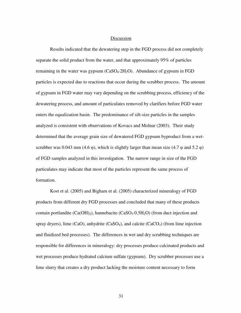
Discussion

Results indicated that the dewatering step in the FGD process did not completely

separate the solid product from the water, and that approximately 95% of particles

remaining in the water was gypsum (CaSO4·2H2O). Abundance of gypsum in FGD

particles is expected due to reactions that occur during the scrubber process. The amount

of gypsum in FGD water may vary depending on the scrubbing process, efficiency of the

dewatering process, and amount of particulates removed by clarifiers before FGD water

enters the equalization basin. The predominance of silt-size particles in the samples

analyzed is consistent with observations of Kovacs and Molnar (2003). Their study

determined that the average grain size of dewatered FGD gypsum byproduct from a wet-

scrubber was 0.043 mm (4.6 φ), which is slightly larger than mean size (4.7 φ and 5.2 φ)

of FGD samples analyzed in this investigation. The narrow range in size of the FGD

particulates may indicate that most of the particles represent the same process of

formation.

Kost et al. (2005) and Bigham et al. (2005) characterized mineralogy of FGD

products from different dry FGD processes and concluded that many of these products

contain portlandite (Ca(OH)2), hannebacite (CaSO3·0.5H2O) (from duct injection and

spray dryers), lime (CaO), anhydrite (CaSO4), and calcite (CaCO3) (from lime injection

and fluidized bed processes). The differences in wet and dry scrubbing techniques are

responsible for differences in mineralogy: dry processes produce calcinated products and

wet processes produce hydrated calcium sulfate (gypsum). Dry scrubber processes use a

lime slurry that creates a dry product lacking the moisture content necessary to form

32

gypsum. Kovacs and Molnar (2003) examined FGD material collected from a wet

scrubber and found that calcite was absent indicating complete conversion to gypsum.

The non-magnetic black FGD particles are interpreted as fly ash because of their

similarity to the non-spherical fly ash particles based on the following properties: color,

shape, surface texture, and chemical composition (Table 2.5). Shape of both particle

types is angular with low sphericity, and both have a pitted surface. The most abundant

elements in both particle types are carbon and oxygen, with trace amounts of aluminum

and silicon present. Because of these similarities, the non-magnetic black FGD particles

are interpreted as fly ash. Külaotos et al. (2003) interpreted particles similar to the non-

magnetic black particles as unburned carbon within coal fly ash.

Based on elemental composition and shape, the magnetic black FGD particles are

similar to magnetic particles within fly ash identified by Hower et al. (1999) and Kukier

(2003). Magnetic fractions of fly ash analyzed in previous studies contain magnetite

(Fe3O4) and hematite (Fe2O3), with smaller fractions of quartz (SiO2) and mullite

(Al6Si2O13) (Hower et al., 1999; Kukier et al., 2003). The major elements represented in

these fly ash minerals are the same as those identified in the magnetic black FGD

particles: iron, silicon, oxygen, and aluminum. Kukier et al. (2003) observed that some

magnetic fly ash particles were “vesiculate and spongy”, which is analogous to the

magnetic black FGD particles described in the current study. We interpret the magnetic

black FGD particles to be magnetic fly ash particles that originated from the coal

combustion chamber, where coal is burned and fly ash is generated (Gieré, 2003).

33

Spherical particles in the fly ash sample and FGD particulate samples (Figure

2.7), including the small spheres attached to FGD particles, are identified as cenospheres

based on similarities in size, shape, surface texture, and elemental composition to

cenospheres described in previous studies (Gieré et al., 2003; Vassilev et al., 2004;

Goodarzi, 2006). Cenospheres are defined as hollow, ceramic microspheres produced

within thermo-electric power plant combustion chambers; size of cenospheres is typically

20-250 µm (Vassilev et al., 2004). Cenospheres found in the FGD particulates of our

study are interpreted to have been transported by flue gas to the scrubber system.

Composition of the cenospheres identified in our investigation is similar to that of

cenospheres analyzed in previous studies (Vassilev et al., 2004; Goodarzi, 2006), with

high concentrations of oxygen, iron, aluminum, silicon, calcium, and magnesium. The

mineral composition of cenospheres includes aluminosilicates, mullite, quartz, calcite, Fe

oxides and Ca silicates (Hulett and Weinberger, 1980; Gieré et al., 2003; Vassilev et al.,

2004).

34

Table 2.5: Characteristics of particle types identified in FGD particulate samples. Fly ash included for comparison. Major

elements (>10%) and minor elements (<10%) are listed from most abundant to least abundant. sa = subangular, sr =

subrounded, FGDS = Flue gas desulfurization scrubber, OC = Uncombusted material from original coal, CCB = Coal

combustion byproduct produced within the coal combustion process

* Many particles were rhombehedral in shape.

** Interpreted from similar size, shape, and elemental composition of coal combustion and FGD byproducts identified in previous studies

(Khanra et. al, 1998; Ma et al., 1999; Sulovsky et. al, 2002; Gieré et al, 2003; Kovacs and Molnar, 2003; Vassilev et al., 2004, Bigham et al.,

2005; Vassilev et al., 2005; Goodarzi, 2006).

Roundness/ Surface Major Minor Interpreted

Particle Type Size Sphericity Texture Elements Elements Identification Origin

White clay-sand rounded/high* smooth divots, O, C, Ca, S Si, Al Gypsum FGDS

indentations

Black

non-magnetic clay-sand sa-sr/low-high pitted, porous C, O Si, Ca, S, Al, Fe, K, F Unburned carbon OC

Magnetic clay-sand sa-sr/low-high pitted, porous C, O, Fe, Si Ca, S, Al, K, Mg, Cl, Ti, Na Magnetic fly ash CCB

Orange silt-sand angular/low uneven O, C, Si, Fe Al, Ca, K, Ti, Mg, S, Mo Iron oxide** CCB

Other

aggregate (rare) silt-sand sa/high --- O, Ca, C Mg, S, Si, Al Limestone** FGDS

sphere (rare) silt rounded/high raised features O, C, Fe Si, Ca, Al, S, Mg, Cenospheres** CCB

flat, Zn rich (rare) sand angular/low uneven C, Zn, O Cl, Fe Fly ash** OC

Fly Ash

smooth, spherical clay-silt rounded/high smooth O, Si, C, Al Fe, K Mullite CCB

pitted, non-spherical sand angular/low-high pitted C, O Si, Al Mullite OC

34

35

Figure 2.7: SEM photomicrographs comparing FGD particles with fly ash. (A) Black

FGD particle with spheres attached. (B) Fly ash sample containing both pitted, non-

spherical particles and smooth, spherical particles. Spheres in both samples are

interpreted as cenospheres formed during coal combustion.

Large iron content (up to 53%) of the orange particles suggests that their color is

caused by the presence of oxidized iron. Iron oxides (hematite), iron spinel (magnetite),

and pyrite (oxidized to limonite/goethite) (Table 2.6) have been identified in previous

studies of fly ash (Khanra et al., 1998; Sulovsky et al., 2002; Vassilev et al., 2005).

Khanra et al. (1998) suggested that the iron-bearing minerals are derived from coal

burned within the combustion chambers of coal-fired power plants. We interpret orange

particles of the FGD particulate samples to have formed within the power plant

combustion chamber and transported by flue gas to the scrubber.

20 µm 10 µm

A B

36

Table 2.6: Typical byproducts from coal combustion and scrubber processes identified in

previous studies (Ma et al., 1999; Gieré et al, 2003; Kovacs and Molnar, 2003; Vassilev

et al., 2004, Bigham et al., 2005; Vassilev et al., 2005). Materials identified in samples of

our study include limestone, gypsum, and mullite. FA = Fly ash, FGD = Flue gas

desulfurization

Byproduct Composition Origin

Gypsum CaSO4 H2O FGD / wet scrubber

Calcite/limestone CaCO3 FGD / lime injection, wet scrubber

Mullite Al6Si2O13 FA / combustion chamber

Portlandite Ca(OH)2 FGD / duct injection, spray dryer process

Hannebachite CaSO3·0.5H2O FGD / duct injection, spray dryer process

Periclase MgO FGD and FA / fluidized bed process

Lime CaO FGD / lime injection

Hematite

(iron oxide) Fe2O3 FA / original coal, combustion chamber

Magnetite

(iron spinel) Fe3O4 FA / original coal, combustion chamber

Quartz SiO2 FA / original coal, combustion chamber

Pyrite FeS2 FA / original coal, combustion chamber

Aluminum oxide

Al2O3

FA / combustion chamber

Based on EDS analysis, the rare subangular aggregate was determined to be

CaCO3. Because CaCO3 is used as the initial material for the FGD reactions, we interpret

the origin of this particle to be from limestone that did not react with elements or

compounds in flue gas during the scrubbing process. The rare, flat, zinc rich particle is

interpreted to be unburned coal or a coal combustion byproduct produced in the coal

combustion chamber. Zinc is commonly found as a trace element within coal fly ash

(Khanra et al., 1998; Pires and Querol, 2004; Vassilev et al., 2004) and as a secondary

inorganic element within coal (Malvadkar et al., 2004).

37

The abundance of carbon associated with FGD particulates determined by EDS

has not been documented by previous research studies. Possible cause may include the

effect from the carbon tape, a film coating across the particle, or added to the particle

during the coal combustion and FGD processes. Effect of the carbon tape is unlikely to

account for the abundance of carbon. Particulates used in this investigation were

approximately 10-30 microns thick and penetration of the EDS is no more than 1 µm.

Evaluation of the points of identification on each particulate showed no correlation

between actual location of the point and carbon content (i.e. closer or further from the

edge of the particle). Particulates were removed from the FGD water that contained a

non-purgeable organic carbon (NPOC) content of 13 to 48 mg/L. This carbon may have

coated the particulates. The formation of the particulates in FGD water includes both

coal combustion and flue gas desulfurization. Carbon is a major component in coal,

exists in the flue gas as carbon dioxide, and is a component of the lime slurry. These

processes may incorporate the carbon into the particulates. Further investigation is

needed to determine the actual source of the carbon determined by EDS in this

investigation.

Disposal or reuse of the large quantity of solid byproducts of the FGD scrubbing

process is an important economic and environmental issue. As environmental air quality

regulations become more stringent, thermo-electric power plants will increasingly

incorporate FGD systems, and the volume of FGD water and associated particulates will

increase. Additional storage and new options for reuse are needed. Coal combustion and

FGD byproducts are being used for cement and construction materials, wallboard,

38

agriculture, and mining (Punshon et al., 1999; Kalyoncu, 2001; Iyer and Scott, 2001,

Laperche and Bigham, 2005; and Yazıcı, 2007). Major factors impacting reuse are purity

of FGD byproducts, state regulations for reuse, toxicity of particulates, and ease of

transporting FGD sludge. Our evaluation indicates that particulates settled from FGD

water are similar to coal combustion and FGD byproducts in terms of physical properties

(size, shape, and texture) and chemical properties (mineral and element content).

Therefore, reuse of FGD particulates that settle in equalization basins of CWTS may be

feasible. However, additional analyses of the FGD particles are needed including a toxic

characteristic leaching procedure (TCLP) and toxicity tests using aquatic organisms.

Conclusions

Three major types of particles were identified in particulate samples from FGD

water. The most abundant particle type is gypsum, which forms during wet scrubbing of

flue gas produced by coal combustion and transported in FGD water to the equalization

basin. Particle size distribution analysis determined that the majority of FGD particulates

are silt size. Other major types are interpreted as fly ash and iron oxide particles, both

produced within the combustion chamber. Multiple particle types present within FGD

particulates originated from both coal combustion and flue gas desulfurization.

39

Acknowledgements: Funding for this research was provided by the U.S. Department of

Energy through the University Coal Research Program.

References

American Coal Ash Association, 2006, CCP Survey, http://www.acaa-usa.org/PDF/

2005_CCP_Production_and_Use_Figures_Released_by_ACAA.pdf. Accessed:

May 2, 2006.

Bigham, J.M., Kost, D.A., Stehouwer, R.C., Beeghly, J.H., Fowler, R., Traina, S.J.,

Wolfe, W.E., and Dick, W.A., 2005, Mineralogical and engineering

characteristics of dry flue gas desulfurization products: Fuel, v. 84, p. 1839-1848.


Company, 184 p.

Founie, A., 2003, Gypsum: U.S. Geological Survey Minerals Yearbook-2003.

Volume I -Metals and Minerals. p. 34.1-34.10.

Gee, G.W. and Bauder, J.W., 1986, Particle-size Analysis, in Klute, A., ed.,

Methods of Soil Analysis, Part I-Physical and Mineralogical Methods

(second edition): Madison, Wisconsin, American Society of Agronomy, Inc., p.

383- 411.

Gieré, R., Carleton, L.E., and Lumpkin, G.R., 2003, Micro-and nanochemistry of fly ash

from a coal-fired power plant: American Mineralogist, v. 88, p. 1853-1865.

Gillespie, W.B. Jr., Hawkins, W.B., Rodgers, J.H. Jr., Cano, M.L., and Dorn, P.B., 2000,

Transfers and transformations of zinc in constructed wetlands: Mitigation of a

refinery effluent: Ecological Engineering, v. 14, p. 279-292.

Goodarzi, F., 2006, Morphology and chemistry of fine particles emitted from a

Canadian coal-fired power plant: Fuel, v. 85, p. 273-280.

Hower, J.C., Rathbone, R.F., Robertson, J.D., Peterson, G., and Trimble, A.S., 1999,

Petrology, mineralogy, and chemistry of magnetically-separated sized fly ash:

Fuel, v. 78, p. 197-203.

Hulett, L.D. and Weinberger, A.J., 1980, Some etching studies of the microstructure and

composition of large aluminosilicate particles in fly ash from coal-burning power

plants: Environmental Science & Technology, v. 14, p.965-969.

40

Iyer, R.S. and Scott, J.A., 2001, Power station fly ash – a review of value-added

utilization outside of the construction industry: Resources, Conservation and

Recycling, v. 31, p. 217-228.

Kalyoncu, R.S., 1999, Coal Combustion Production. U.S. Geological Survey

MineralsYearbook-1999, p. 19.1-19.4.

Khanra, S., Mallick, D., Dutta, S.N., and Chaudhuri, S.K., 1998, Studies on the phase

mineralogy and leaching characteristics of coal fly ash: Water, Air, and Soil

Pollution, v. 107, p. 251-275.

Knight, R.L., Kadlec, R.H., and Ohlendorf, H.M., 1999, The use of treatment

wetlands for petroleum industry effluents: Environmental Science &

Technology, v. 33, p. 973-980.

Kost, D.A., Bigham, J.M., Stehouwer, C., Beeghly, J.H., Fowler, R., Traina, S.J., Wolfe,

W.E., and Dick, W.A., 2005, Chemical and physical properties of dry flue gas

desulfurization products: Journal of Environmental Quality, v. 34, p. 676-686.

Kovacs, F. and Molnar, J., 2003, Basic properties of flue-gas desulfurization

gypsum: Acta Montanistica Slovaca, v. 8, p. 16-19.

Kukier, U., Ishak, C. F., Sumner, M.E., and Miller, W.P., 2003, Composition and

element solubility of magnetic and non-magnetic fly ash fractions: Environmental

Pollution, v. 123, p. 255-266.

Külaots, I., Hurt, R.H., and Suuberg, E.M., 2004, Size distribution of unburned carbon in

coal fly ash and its implications: Fuel, v. 83, p. 223-230.

Laperche, V. and Bigham, J.M., 2002, Quantitative, chemical, and mineralogical

characterization of flue gas desulfurization by-products: Journal of Environmental

Quality, v. 31, p. 979-987.

Ma, B, Qi, M., Peng, J., and Li, Z., 1999, The compositions, surface texture, absorption,

and binding properties of fly ash in China: Environment International, v. 25, p.

423-432.

Malvadkar, S.B., Forbes, S., McGurl, G.V., 2004, Formation of Coal Resources:

Encyclopedia of Energy, v. 1, p. 529-550.

41

McCarthey, J., Dopatka, J., Mardini, R.H., Rader, P., and Bussell, C., 2005, Duke Power

WFGD Retrofit Program: Compliance via Standardization and Selective Site-

specific Innovations, POWER-GEN International 2005. Las Vegas, NV, 29 p.

Available: <http://www.power.alstom.com/home/events/past_events/

power_gen_international/_files/file_20379_56769.pdf>

Mierzejewski, M.K., 1991, The Elimination of Pollutants from FGD waters, The 1991

SO2 Control Symposium. Washington D.C. 20 p.

Mooney, D., Rodgers, J.H. Jr., Murray-Gulde, C., Huddleston, G.M., III, 2006,



Programs, p. 18.

Murray-Gulde, C.L., Bearr, J., and Rodgers, J.H. Jr., 2003a, Evaluation of a

constructed wetland treatment system specifically designed to decrease

bioavailable copper in a waste stream: Ecotoxicology and Environmental Safety,

v. 61, p. 60-73.

Murray-Gulde, C., Heatley, J.E., Karanfil, T., Rodgers, J.H. Jr., and Myers, J.E. 2003b.

Performance of a hybrid reverse osmosis-constructed wetland treatment system

for brackish oil field produced water: Water Research, v. 37, p. 705-713.

Pires, M. and Querol, X., 2004, Characterization of Candiota (South Brazil) coal and

combustion by-product: International Journal of Coal Geology, v. 60, p. 57-72.

Poppe, L.J., Paskevich, V.F., Hathaway, J.C., and Blackwood, D.S., 2001, A

Laboratory Manual for X-Ray Powder Diffraction: U.S. Geological Survey Open-

File Report 01-041, CD-Rom.

Powers, M.C., 1953, A new roundness scale for sedimentary particles: Journal of

Sedimentary Petrology, v. 23, p. 117-119.

Punshon, T., Knox, A.S., Adriano, D.C., Seaman, J.C., and Weber, J.T., 1999, Flue gas

desulfurization (FGD) residue: Potential applications and environmental issues in

Sajwan, K.S., Alva, A.K., and Keefer, R.F., eds., Biogeochemistry of trace

elements in coal and coal combustion byproducts: New York, Kluwer

Academic/Plenum Publishers, p. 7-28.

Schweinfurth, S.P., 2005, Coal - A complex natural resource: U.S. Geological

Survey, Circular 1143, 39 p.

Sulovsky, P., 2002, Mineralogy and chemistry of conventional and fluidized bed coal

ashes: Bulletin of the Czech Geological Survey, v. 77, p. 1-11.

42

Termuehlen, H. and Emsperger, W., 2003, Clean and Efficient Coal-Fired Power Plants:

New York, ASME Press, 143 p.

Vassilev, S.V., Menendez, R., Diaz-Somoano, M., Tarazona-Martinez, M.R., 2004,

Phase-mineral and chemical composition of coal fly ashes as a basis for their

mulitcomponent utilization. 2. Characterization of ceramic cenosphere and salt

concentrates: Fuel, v. 83, p. 585-603.

Vassilev, S.V., Vassileva, C.G., Karayigit, A.I., Bulut, Y., Alastuey, A., and

Querol, X., 2005, Phase-mineral and chemical composition of fractions

separated from composite fly ashes at the Soma power station, Turkey:

International Journal of Coal Geology, v.61, no.1-2, p. 65-85.

Wentworth, C.K., 1922, A scale of grade and class terms for clastic sediment:

Journal of Geology, v. 30, p. 377-393.

Yazıcı, H., 2007, Utilization of coal combustion byproducts in building blocks: Fuel, v.

86, p. 929-937.

43

CHAPTER III

THE ROLE OF AN EQUALIZATION BASIN IN

A CONSTRUCTED WETLAND TREATMENT SYSTEM

Abstract

Laboratory analyses were performed to investigate the role of equalization basins

in the treatment of flue gas desulfurization (FGD) water by constructed wetland treatment

systems (CWTS). Pilot-scale equalization basins were used to evaluate the removal of

constituents of concern (Hg, As, and Se) and toxicity of FGD water. Hg, As, and Se

concentrations were measured in FGD water and in particles suspended within the water.

Settling analysis using Stokes’ Law was performed to determine size distribution and

settling rates of FGD particles. Analysis of FGD water samples indicated that aqueous

concentrations of Hg, As, and Se and toxicity remained constant or changed very slightly

in the pilot-scale equalization basins during a 24 hr hydraulic retention time. FGD

particles were predominantly silt size, and approximately 99% of particles suspended in

FGD water settled to the bottom of a 2.5 m deep equalization basin within the first 4 hrs

of the 24 hr hydraulic retention time. As the particles settled the Hg, As, and Se in these

particles were removed from the water column. Approximately 90% of the total As

concentration (water and particles) was removed by particle settling in the equalization

basin. This investigation supports the use of equalization basins for treatment of FGD

waters in CWTS, specifically to settle particles.

44

Introduction

The purpose of this investigation was to examine the role of equalization basins as

a component of constructed wetland treatment systems (CWTS) designed to treat flue gas

desulfurization (FGD) water. Equalization basins are constructed retention pools used to

store water and are the primary step in many water treatment systems. Equalization

basins have retained waters including sewage, ash sluice, surface mine, and surface

runoff waters (Cherry et al., 1984; Greenburg, 1986; Somes et al., 2000).

Specifically designed CWTS are used in industry to effectively treat several types

of waters including municipal wastewater, acid mine drainage, pulp mill effluent, refinery

effluent, agricultural waste, urban runoff, and landfill leachate (Watson et al., 1989).

CWTS are designed to promote specific reactions for the transfer or transformation of

inorganic and organic constituents to non-bioavailable forms (Knight et al., 1999;

Gillespie et al., 2000; Murray-Gulde et al., 2003a; 2003b). The most important design

components are hydrosoil, macrophytes (plants), and hydroperiod (hydraulic retention

time).

Flue gas desulfurization, the process of removing sulfur dioxide and other harmful

vapors from flue gas of coal combustion chambers, is an innovative technology used by

coal-fired power plants to meet U.S. Environmental Protection Agency (USEPA)

standards for air emissions. In the United States, 85% of operating FGD systems are wet-

limestone based scrubbers (USEPA, 2003). Wet-limestone scrubbers use a slurry of

water, limestone, and organic acids to react with sulfur dioxide to form calcium sulfite

45

(CaSO3) (Equation 1), which when further oxidized forms calcium sulfate (CaSO4)

(Equation 2) (Mierzejewski, 1991; Laperche and Bigham, 2002).

SO2 + CaCO3 + H2O CaSO3·0.5H2O + CO2 + 0.5H2O Equation 3.1

CaSO3·0.5H2O + 0.5O2 + 1.5H2O CaSO4·2H2O Equation 3.2

The slurry is dewatered by belt presses, vacuum filtration, or centrifugation. The

resulting solid product is composed primarily of gypsum (CaSO4·2H2O).

Water produced by dewatering the slurry is typically high in chlorides, sulfates,

total suspended solids, and other constituents released from coal combustion and

scrubbing processes. Mercury (Hg), arsenic (As), and selenium (Se) are the major

inorganic constituents of concern within FGD water due to their toxicity to aquatic

organisms and concentrations that exceed EPA discharge limits. Other inorganic

elements that may be of concern in FGD water include copper, zinc, lead, boron, nickel,

cobalt, iron, and magnesium (Arrington, 2005).

Design of equalization basins is based on factors such as power plant size, local

regulatory policy, site conditions, engineer’s judgment and experience, and economics

(WEF and ASCE, 1992). Parameters for an equalization basin designed to store FGD

water also include the amount of water produced and holding period for the water. In a

single North Carolina coal-fired power plant, the scrubber generates up to 1.75 million

gallons of FGD water per day (Mooney et al., 2006). The hydraulic retention time (HRT)

for FGD water in an equalization basin is generally 24 hrs.

46

Equalization basins for CWTS provide storage for particles to settle and for

cooling and homogenizing of FGD water prior to entering CWTS reactors. The

temperature of FGD water entering an equalization basin is approximately 40°C

(Mierzejewski, 1991; Doug Mooney, 2006 written communication). This water is cooled

to approximately 35°C to avoid exposing macrophytes in the CWTS reactors to high

temperatures. Particle concentrations (total suspended solids) in FGD water in an

equalization basin of a CWTS can vary depending on the dewatering and clarifier

techniques, but may average approximately 1,000 mg/L (Doug Mooney, 2006 written

communication). Settling of particles in the equalization basin increases longevity of the

CWTS by reducing the volume of solid material entering the wetland reactors.

Methods of removing constituents of concern in FGD water may include both

chemical and physical processes, including particle settling within equalization basins.

However, these processes in equalization basins have not been adequately studied. To

date, there has been no documented treatment (transfers or transformations) of

constituents in FGD water attributed to equalization basins.

The purpose of the current research was to investigate physical processes of

treatment that may occur within equalization basins of CWTS used to treat FGD water.

Specific objectives of the research were (1) to determine settling rates for FGD particles

within an equalization basin; (2) to determine if removal of Hg, As, and Se occurs within

an equalization basin by measuring change in concentrations over time; and (3) to

determine if toxicity of FGD water changes within an equalization basin during a 24 hr

HRT.

47

Methods

Samples Analyzed

Six FGD waters were obtained from three coal-fired power plants located in the

South Eastern United States: four from a pilot-scale wet scrubber and two from full-scale

wet scrubbers (Table 3.1). Each of the pilot-scale scrubber waters represented

combustion of a different coal. All waters were delivered to Clemson University by

tanker truck. FGD particles used in this study were collected from two of the pilot-scale

waters (Table 3.1) from the bottom valve opening of the tanker truck after the contents

had settled for approximately two days.

All FGD waters were diluted with municipal water to achieve a chloride

concentration of approximately 4,000 mg/L. In a full-scale equalization basin of a

CWTS, water must be diluted to this chloride concentration to eliminate negative effects

to macrophytes of the wetland system (McCarthey et. al, 2005). Therefore, in order to

provide results representative of full-scale equalization basins, data presented in this

paper are for diluted FGD waters. In addition, general water chemistry was measured on

FGD water samples prior to dilution.

48

Table 3.1: Analyses performed for waters and particles. PSD = Particle size distribution,

D = Density, V= Viscosity

Analyses

Water Aqueous Particle

ID (Source) PSD D and V Chem. Chem. Toxicity

FGD Waters

PS-1 (Pilot-scale scrubber) X




FS-A (Full-scale scrubber) X X X

FS-B (Full-scale scrubber) X X X

FGD Particle Samples

BP-3 (from Water PS-3) X

BP-4 (from Water PS-4) X

PFS-A (added to Water FS-A)* X

PFS-B (added to Water FS-B)* X

* Particles from BP-4 were added to waters FS-A and FS-B to simulate particle concentrations in FGD waters of

equalization basins of CWTS.

Particle Size and Settling Rates

The pipette method (Folk, 1980) was used to determine particle size distribution

of FGD particle samples (Table 3.1). Sand-size particles were separated from samples

BP-3 and BP-4 using a 62.5 µm sieve, then dried and weighed. Remaining silt and clay-

size particles were suspended in de-ionized water in a 1,000 mL graduated cylinder, and

20 mL samples were withdrawn at specific times. Using methodology of Folk (1980),

grain size diameter was calculated for each 20 mL sample withdrawn using a particle

density for gypsum (2.32 g/cm³), which is the most common (approximately 95%)

49

mineral in FGD particles based on results of this investigation. Cumulative particle size

distribution curves were constructed from weights of the size fractions.

To determine settling rates of particles within actual FGD water, Stokes’ Law was

applied (Gee and Bauder, 1986). The settling velocities corresponding to selected

particle diameters were calculated using Equation 3:

Equation 3.3

where v is the settling velocity of particles (cm/s), g is the acceleration due to gravity

(cm/s²), ρs is the particle density (g/cm³), ρl is the fluid density (g/cm³), X is the particle

diameter (cm), and η is fluid viscosity (g/cm-sec).

A particle density of 2.32 g/cm³ (gypsum) was used in Equation 3. The viscosity

of waters FS-A and FS-B was measured using a Cannon-Fenske Opaque Viscometer

according to ASTM methods D445 and D446 (2001) for glass capillary kinematic

viscometers. Fluid density was measured by weighing 1 mL of FGD water using a

calibrated pipette. All measurements were performed at 22ºC water temperature

(ambient room temperature), which eliminates effects of heating or cooling of water

during experiments. Settling velocities were calculated for particle diameters at 0.5 φ

intervals between 5 and 9 φ and 0.25 φ intervals between 4 and 5 φ. The value of φ is

calculated by Equation 4 (Krumbein, 1936),

Equation 3.4

ηρρ

18

)( 2Xg

v ls −=

( )d2log−=ϕ

50

where d is the grain size diameter (mm). The calculated settling velocities were used to

determine the time required for each particle size to reach the bottom of an equalization

basin with a depth of 2.5 m, a typical depth of equalization basins.

Water Chemistry

Pilot-Scale Scrubber Waters

Pilot-scale scrubber waters (Table 3.1) were analyzed to determine if storage of

FGD water in an equalization basin influences Hg, As, and Se concentrations over a 24 hr

hydraulic retention time (HRT). The HRT was selected based on the holding period of

water in full-scale equalization basins of CWTS. Each FGD water (PS-1 to PS-4) was

diluted to achieve a chloride concentration of approximately 4,000 mg/L in a 3,780 L

polypropylene pilot-scale equalization basin and then circulated using a submersible

pump. Samples (“initial samples”) were collected in 1 L HDPE bottles immediately after

contents of the equalization basin were thoroughly mixed and the submersible pump was

turned off (Figure 3.1). Two water samples (“final samples”) were collected 24 hrs later

at the equalization basin outflow prior to entering the wetland reactors of two separate

treatment series. Values from analysis of the two final samples were averaged for each

water. Conductivity, pH, alkalinity, hardness, dissolved oxygen, chloride , and sulfate

concentrations were measured for each water (Table 3.2). Initial and final samples from

each of the four pilot-scale waters were analyzed for Hg, As, and Se by ICP-MS (Perkin

Elmer, Sciex Elan 9000).

51

Figure 3.1: A) Pilot-scale 3,780 L equalization basin. B) Schematic showing sampling

locations for initial and final samples of waters PS-1 through PS-4.

Table 3.2: Methods for general water chemistry and inorganic analysis.

Parameter Method Detection Limit

pH Direct Instrumentation: Orion Model 420A 0.01

Conductivity Direct Instrumentation: YSI 30 0.1 mS

Alkalinity Standard Methods: 2320 B (APHA, 1998) 2 mg/L as CaCO3

Hardness Standard Methods: 2340 C (APHA, 1998) 2 mg/L as CaCO3

DO1 Direct Instrumentation: YSI Model 52 0.1 mg/L

Chloride HACH Colorimetric Method 8207 25 mg/L

Sulfate Standard Methods: 4500 E (APHA, 1998) 1.0 mg/L

Se2, As

2 Inductively Coupled Plasma with Mass

Spectrometry (ICP-MS): USEPA 200.8 1.0 µg/L

Hg2 (ICP-MS): USEPA 200.8 0.1 µg/L

Hg3, As

3, Se

3 Atomic Fluorescence Spectroscopy (AFS)

(Aurora Instruments, AI 3200) 1.0 µg/L

1 Dissolved Oxygen

2 Used for pilot-scale scrubber waters

3 Used for full-scale scrubber water and digested particle samples

Equalization

Basin

First Reactor of

Pilot-scale CWTS

Initial Samples

Pump

Final Samples

A B

52

Water and Particle Chemistry

Full-Scale Scrubber Waters

Full-scale scrubber water (FS-A and FS-B) was diluted to approximately 4,000

mg/L chlorides in a static, 73 L rectangular storage bin used as a pilot-scale equalization

basin. A representative split of particle sample BP-4 was added within the 73 L bin to

waters FS-A and FS-B to create water with a particle concentration (1,000 mg/L) typical

of full-scale equalization basins used with CWTS. To fully suspend particles in the water

column, the FGD water and particles were mixed for approximately one minute. Water

samples (“initial samples”) were collected immediately after mixing to simulate water

entering an equalization basin. Water samples (“final samples”) were collected after 24

hrs to simulate water leaving an equalization basin after a 24 hr HRT.

General water chemistry analyses were performed on initial and final samples of

the full scale scrubber waters (Table 3.2). A 200 mL aliquot of initial and final samples

from waters FS-A and FS-B was filtered through a 0.45 µm filter to separate the particles.

The water was preserved using nitric acid (trace metal grade) for measurement of Hg, As,

and Se concentrations. Following methods outlined by Hatanpää et al. (1997), particles

(samples PFS-A and PFS-B) collected on the filter paper were dried, weighed, and

digested. Although both initial and final samples were filtered, the final samples

contained too few particles for analysis, and therefore only particles collected from the

initial samples were digested. FGD particles were digested for As and Se analysis in

closed Teflon PFA vessels in a microwave oven (Mars5 System, CEM model) using 10

mL nitric acid (HNO3 , Certified ACS Plus). FGD particles were digested for Hg analysis

using 10 mL nitric acid and 5 mL sulfuric acid (H2SO4, Certified ACS Plus) under a

53

reflux condenser. The full-scale scrubber waters and digested particle samples were

analyzed for Hg, As, and Se by atomic fluorescence spectroscopy (AFS) (Aurora

Instruments, AI 3200).

To determine the cumulative removal of Hg, As, and Se associated with particles

settling from the water column, it was assumed that the constituents were distributed

evenly among all particle sizes. Therefore, the removal rate of constituents is

proportional to the mass of particles settled. Removal rates for Hg, As, and Se associated

with particles during settling were estimated using a two point slope estimation

performed on the data for constituent concentration over time:

where R is the removal rate of constituents [(µg/L)/hr], C is the concentration of the

constituent (µg/L), t is time (hrs), and n is the data point.

Toxicity Experiments

Toxicity of initial samples was compared to that of final samples for waters FS-A

and FS-B using a standard 7-day static/renewal toxicity test following USEPA methods

(Lewis et al., 1994). The test organism, Ceriodaphnia dubia (a water flea), is commonly

used for toxicity testing in the United States (Lewis et al., 1994). Toxicity endpoints for

the C. dubia experiments were mortality and reproduction. To remove the effect of

chloride on toxicity, chloride concentrations were reduced to below the no observable

effect concentration (NOEC). A series of dilutions for FS-A and FS-B, initial and final,

nn

nn

tt

CCR

−−=

+

+

1

1 Equation 3.5

54

were prepared with moderately hard water (70 mg/L as CaCO3). Chloride concentrations

after dilution for each water sample were 500, 300, 150, 75, and 50 mg/L Cl-. All

dilution treatments were compared to a control of moderately hard water. To determine

differences in survival data between initial and final sampling, a Chi-Square Analysis

using critical values from Fishers Exact Test (α = 0.05) was performed. C. dubia

reproductive data were evaluated in comparison to control organisms using a one-way

analysis of variance test (ANOVA; α = 0.05) and mean separation using a least

significant difference test (LSD). General water chemistry analyses, including pH,

conductivity, hardness, alkalinity, and dissolved oxygen were conducted on days 1, 3, 5,

and 7 of the toxicity experiments. These data were used to determine if mortality was

affected by changes in general water chemistry.

Results

Size and Settling Rates of FGD Particles

FGD particles analyzed consist predominantly of silt-size material (between 4 and

9 φ) (Figure 3.2, Table 3.3). The graphic mean size of sample BP-3 is 5.3 φ with an

inclusive graphic standard deviation of 0.34 φ, indicating very well sorted medium silt.

Graphic mean size of sample BP-4 is 4.7 φ with an inclusive graphic standard deviation

of 0.29 φ, indicating very well sorted coarse silt. The size distribution of both particle

samples is unimodal and nearly symmetrical.

Values of dynamic viscosity measured for waters FS-A and FS-B are 0.0099

g/cm-sec and 0.0103 g/cm-sec, respectively. The measured fluid densities of FS-A and

55

FS-B are 1.010 g/cm³ and 1.013 g/cm³, respectively. The settling rate of particles

calculated by Stokes’ Law in water FS-A is slightly greater than that for water FS-B

(Table 3.3) because of minor differences in viscosity and density between the two waters.

Using the calculated settling rates and the measured particle size distributions,

greater than 98% of particles settle to the bottom of a 2.5 m deep equalization basin of a

CWTS within a 24 hr HRT (Table 3.3). This indicates that the typical HRT within an

equalization basin is adequate to remove nearly all of the suspended particles. For

sample BP-4, 78% of the particles settle within the first hour (Figure 3.3, Table 3.3).

Because the particle size is slightly finer in sample BP-3, more time is required for

settling, with approximately 73% of the articles removed from suspension during the

second hour of settling.

56

Figure 3.2: Cumulative size distribution curves for FGD particle samples.

A) Sample BP-3. B) Sample BP-4.

A

7 9

0

20

40

60

80

100

4 5 6 7 8

Cum

ula

tive

%

B

Grain Diameter (φ)

4 5 6 7 8 9

0

20

40

60

80

100

4 5 6 7 8 9

0

20

40

60

80

100

Grain Diameter (φ)

Cu

mu

lati

ve

%

14

Table 3.3: Size distribution measured in FGD particle samples BP-3 and BP-4; settling rates (cm/s) and settling times (hrs)

calculated using Stokes’ Law; and measured viscosity and density of waters FS-A and FS-B. Times calculated for settling to

the bottom of a 2.5 m deep equalization basin.

Size Distribution Settling Rate Settling Time

Grain Diameter Wentworth (1922) (Cumulative %) (cm/s) (hrs)

(mm) (φ) Size Class BP-3 BP-4 FS-A FS-B FS-A FS-B

0.0625 4 v. fine sand 0.65 2.27 0.28 0.27 0.25 0.26

0.053 4.25 coarse silt 3.05 6.90 0.20 0.19 0.34 0.36

0.044 4.5 coarse silt 5.10 18.5 0.14 0.13 0.50 0.52

0.037 4.75 coarse silt 7.41 52.2 0.099 0.095 0.70 0.73

0.031 5 coarse silt 14.5 78.1 0.070 0.067 1.00 1.04

0.022 5.5 medium silt 87.1 96.6 0.035 0.034 1.98 2.07

0.016 6 medium silt 96.5 97.8 0.019 0.018 3.75 3.90

0.011 6.5 medium silt 98.0 99.1 0.0088 0.0084 7.93 8.26

0.0078 7 fine silt 98.5 99.3 0.0044 0.0042 15.8 16.4

0.0055 7.5 fine silt 99.0 99.5 0.0022 0.0021 31.7 33.0

0.0039 8 v. fine silt 99.0 99.8 0.0011 0.0010 63.1 65.7

0.0028 8.5 v. fine silt 99.1 99.8 0.00057 0.00054 122 127

0.0020 9 clay 99.1 99.9 0.00029 0.00028 240 250

57

58

Figure 3.3: Cumulative percent removal of FGD particles in an equalization basin with a

depth of 2.5 m. Based on settling rates calculated from particle size distribution

measured for particle samples BP-3 and BP-4 and viscosity and density measured for

waters FS-A and FS-B (Figure 3.2 and Table 3.4) A) Sample BP-3. B) Sample BP-4.

0

10

20

30

40

50

60

70

80

90

100

0 0.5 1 1.5 2 2.5 3 3.5 4

Removal Time (hrs)

Cu

mu

lati

ve

% R

emo

va

l

.

0

10

20

30

40

50

60

70

80

90

100

0 0.5 1 1.5 2 2.5 3 3.5 4

Removal Time (hrs)

Cu

mu

lati

ve

% R

emo

val

.

A

B

FS-A FS-B

59

Water Chemistry

Pilot-Scale Scrubber Waters

General water chemistry values for the pilot-scale scrubber waters prior to

dilution are listed in Table 3.4. Following dilution to achieve targeted chloride

concentrations representative of equalization basins of CWTS, general water chemistry

values for initial samples of the pilot-scale scrubber waters (PS-1 to PS-4) were: 8.66 to

9.09 mg/L dissolved oxygen, 6.79 to 7.11 (su) pH, 24 to 46 mg/L (as CaCO3) alkalinity,

4,200 to 9,800 mg/L (as CaCO3) hardness, 10.1 to 12.0 mS conductivity, and 1,250 to

1,610 mg/L sulfate. The general water chemistry of final samples is similar to that of

initial samples (Table 3.5).

Mercury concentrations in initial samples of pilot-scale scrubber waters (PS-1 to

PS-4) in the equalization basin ranged from 0.4 to 43 µg/L (Table 3.5). Decrease in

mercury concentration from initial to final samples was observed for two of the four

waters (PS-1 and PS-2). The highest initial mercury concentration (43 µg/L in PS-2)

decreased to a final concentration of 22 µg/L, resulting in 49% removal of mercury.

Initial concentration for PS-1 was 0.9 µg/L Hg, and the final concentration decreased by

0.3 µg/L, resulting in 33% removal. The only removal of arsenic from the pilot-scale

scrubber water within the equalization basin was 1 µg/L (2.8%) in PS-4. Selenium

concentrations in initial samples of pilot-scale scrubber water ranged from 610 µg/L to

2,980 µg/L. Decrease in Se concentration from initial to final samples was observed for

three of the four waters. The highest initial selenium concentration (2,980 µg/L in PS-2)

decreased to a final concentration of 2,750 µg/L, resulting in 7.7% removal. Initial

selenium concentrations for PS-1 and PS-4 were 610 µg/L and 650 µg/L, respectively.

60

Percent removal of Se was 1.2% (7 µg/L decrease) for PS-1 and 3.4% (22 µg/L decrease)

for PS-4.

Water Chemistry and Particle Analysis

Full-Scale Scrubber Waters

General water chemistry values for the full-scale scrubber waters prior to dilution

are listed in Table 3.4. Following dilution, general water chemistry values for initial

samples of the full-scale scrubber waters (FS-A and FS-B) were: 7.96 mg/L dissolved

oxygen, 6.83 to 7.69 (su) pH, 2,800 to 4,000 mg/L (as CaCO3) hardness, 11.0 to 13.2 mS

conductivity, and 890 to 980 mg/L sulfate. Alkalinity values differed between the initial

samples: 18 mg/L (CaCO3) for FS-A and 220 mg/L for FS-B. General water chemistry

of final samples did not differ from that of initial samples (Table 3.5).

Arsenic concentrations in the aqueous phase of initial samples of the full-scale

scrubber waters were 2.68 µg/L in FS-A and 2.02 µg/L in FS-B (Table 3.5). Initial

selenium concentrations in the aqueous phase were 1350 µg/L in FS-A and 1440 µg/L in

FS-B. Aqueous mercury concentration in the initial sample for FS-A was 12.9 µg/L,

while the aqueous mercury concentration in FS-B was below the detection limit (less than

1.0 µg/L). A decrease of approximately 1 µg/L of Hg was observed in FS-A. Selenium

removal was 10% in FS-A with approximately 2% removal from FS-B. There was no

removal of As from either water.

Table 3.4: General water chemistry for the six FGD waters used in this investigation prior to dilution and parameter ranges for

full-scale scrubber FGD waters characterized by Mierzejewski (1991) and Arrington (2005). ND = Not determined FGD Waters

Parameter Units PS-1 PS-2 PS-3 PS-4 FS-A FS-B Arrington Mierzejewski

pH Su 7.1 ND 7.3 7.4 6.6 7.5 6 - 7 4 - 7

Alkalinity mg/L¹ 84 ND 56 46 26 840 152 - 600 ND

Hardness mg/L¹ 3200 5000 8000 7200 10500 14000 10400 – 24800 ND

Conductivity mS 13.3 12.8 14.3 13.1 19.7 42 20.3 – 36.3 ND

Chloride mg/L 5375 5250 5750 5350 14200 21000 1640 – 15900 10000 – 40000

¹ mg/L as CaCO3

Table 3.5: General water chemistry and concentrations of Hg, As, and Se for pilot-scale scrubber waters (PS-1 to PS-4) and

full-scale scrubber waters (FS-A and FS-B) following dilution. DO = Dissolved oxygen, BDL = Below detection limit (1 µg/L)

Waters and Samples

Parameters and PS-1 PS-2 PS-3 PS-4 FS-A FS-B

Constituents Units Initial Final1 Initial Final

1 Initial Final

1 Initial Final

1 Initial Final Initial Final

DO mg/L 8.66 7.87 9.09 8.84 9.00 8.94 8.66 8.26 7.96 9.40 7.96 6.90

pH su 7.00 7.00 6.79 6.77 7.10 7.00 7.11 7.09 6.83 6.86 7.69 7.65

Alkalinity mg/L¹ 46 45 26 24 32 33 24 25 18 20 220 210

Hardness mg/L¹ 4200 3800 9800 6000 6400 7800 6400 6100 2800 3100 4000 3800

Conductivity mS 10.1 10.0 10.9 10.9 12.0 12.2 11.7 11.6 11.0 11.2 13.2 13.3

Chloride mg/L 3150 3375 3550 3490 4230 4330 4050 4200 4280 4200 5000 5025

Sulfate mg/L 1610 1490 1520 1390 1360 1350 1250 1260 980 1030 890 910

Mercury µg/L 0.9 0.6 43 22 36 44 0.4 0.4 12.9 12.0 BDL BDL

Arsenic µg/L 4.7 5.7 101 124 47 50 35 34 2.68 3.67 2.02 2.08

Selenium µg/L 610 603 2980 2750 2100 2220 650 628 1350 1220 1440 1400 1 Final values are averaged from two water samples, one for each outflow (see Methods) 2 mg/L as CaCO3

61

62

Mercury content of particle samples PFS-A and PFS-B was 0.91 and 1.2 µg/g,

respectively. Arsenic content in PFS-A and PFS-B was 19 and 21 µg/g. Selenium

content differed between particle samples PFS-A and PFS-B at 45 µg/g and 19 µg/g,

respectively. Because each liter of water in the equalization basin contained 1 g of

particles, the amount of mercury in waters FS-A and FS-B waters due to particle content

was 0.91 and 1.2 µg/L, respectively. Arsenic content due to particles was 19 µg/L in FS-

A and 21 µg/L in FS-B. Selenium content due to particles in FS-A and FS-B was 45

µg/L and 19 µg/L, respectively. Over time, Hg, As, and Se associated with particles in

the water are removed by settling of FGD particles to the bottom of the equalization basin

(Figure 3.4).

The calculated removal rates (Table 3.6) indicate the time at which maximum

removal of constituents occurs by particle settling in an equalization basin. These rates

show that maximum removal of Hg, As, and Se associated with particles occurs

approximately 0.6 hrs after the start of the HRT for both waters FS-A and FS-B. After

approximately 2.4 hours, the removal rates are two orders of magnitude less than the

maximum, which indicates that by this time further removal of constituents is negligible.

63

Figure 3.4: Mass of Hg, As, and Se (µg) removed per liter of water by particle settling,

assuming a particle concentration of 1,000 mg/L. Change in concentration with settling

time is based on particle settling rates, content of Hg, As, and Se in particles, and a 2.5 m

depth of basin. Points on each graph represent known settling times for φ values used to

construct the cumulative size distribution curves (Figure 3.2). Time = 0 represents water

entering the equalization basin.

64

Table 3.6: Removal rates of Hg, As, and Se by particle settling in FS-A and FS-B for an

equalization basin depth of 2.5 m based on a two-point slope estimation (Equation 5) of

the known points used to construct the concentration curves (Figure 3.4).

FS-A Removal Rates [(µg/L)/hr]

Time (hrs) Hg As Se

0.32 0.36 7.7 18

0.60 1.3 28 66

1.2 0.33 7.0 16

2.3 0.017 0.35 0.82

4.7 0.0025 0.054 0.13

9.5 0.00076 0.016 0.037

FS-B Removal Rates [(µg/L)/hr]

Time (hrs) Hg As Se

0.33 0.47 8.0 7.3

0.62 1.7 29 27

1.2 0.43 7.3 6.6

2.4 0.021 0.36 0.33

4.9 0.0033 0.056 0.051

9.9 0.0010 0.017 0.015

Toxicity

Survival of C. dubia was affected by exposure to water FS-A at chloride dilutions

of 300 and 500 mg/L Cl- (Figure 3.5A). At 500 mg/L Cl

-, exposure to initial samples

resulted in 50% survival, and exposure to final samples resulted in 70% survival.

Exposures at 300 mg/L Cl- resulted in 70% survival for initial samples, and C. dubia was

not affected (100% survival) by final samples. Initial and final samples for the dilutions

of 150, 75, and 50 mg/L Cl- did not affect survival of C. dubia. Reproduction of C. dubia

was impaired at the 300 and 500 mg/L Cl- dilutions of initial and final samples compared

to the control (Figure 3.5B). Reproduction of C. dubia was not affected by initial or final

65

samples for chloride concentrations of 50 and 75 mg/L. Treatment of water by the

equalization basin was suggested only by survival for the 300 mg/L Cl- dilution;

however, treatment was not seen in terms of reproduction for this dilution.

Survival of C. dubia was affected by exposure to water FS-B at 150, 300, and 500

mg/L Cl- dilutions. Both initial and final samples resulted in toxicity for all three

dilutions. Exposures at 500 mg/L Cl- resulted in 100% mortality in initial and final

samples (Figure 3.5C). At 300 mg/L Cl-, exposure to initial samples resulted in 20%

survival, and exposure to final samples resulted in 10% survival. Exposures at 150 mg/L

Cl- resulted in 60% survival in both initial and final samples. Reproduction of C. dubia

was impaired for both initial and final samples at all chloride dilutions to the extent that

no reproduction occurred. The pilot-scale equalization basin did not affect toxicity of

water FS-B to C. dubia during the 24 hr HRT.

66

Figure 3.5: Response of C. dubia to full-scale scrubber waters. A) Survival after

exposure to water FS-A. B) Reproduction after exposure to water FS-A. C) Survival after

exposure to water FS-B. Reproduction did not occur for organisms exposed to FS-B.

A

0

2

0

4

0

6

0

8

0

100

Control 50 75 150 300 500

Su

rviv

al

(%)

Chloride Concentration of FGD Water (mg/L)

0

5

10

15

20

25

30

35

Control 50 75 150 300 500


Rep

rod

uct

ion

(Mea

n N

eon

ate

s /

Ad

ult

)

0

20

40

60

80

100

Control 50 75 150 300 500


Su

rviv

al

(%)

Control Final Samples Initial Samples

B

C

67

Discussion

Two mechanisms of potential treatment within equalization basins of constructed

wetland systems were investigated for FGD waters: treatment by decrease in aqueous

concentrations of constituents of concern (Hg, As, and Se) and treatment by particle

settling. To determine treatment of FGD waters, concentrations of initial and final

samples of each water were analyzed and toxicity experiments were used.

Treatment of aqueous phase constituents of concern in FGD waters of an

equalization basin ranged from no removal to approximately 50% removal. The

maximum removal of constituents of concern in the aqueous phase was observed for

water PS-2. During a 24 HRT, Hg concentration in water PS-2 decreased from 43 µg/L

to 22 µg/L and Se concentration from 2980 µg/L to 2750 µg/L. For the other FGD

scrubber waters, removal in the equalization basin was 3 µg/L or less Hg and 130 µg/L or

less Se. Removal of As from the aqueous phase within the pilot-scale equalization basins

did not occur. The results of toxicity tests using C. dubia suggest that no decrease in

toxicity of FGD water occurs within the equalization basin. Biogeochemical pathways

for the transfer or transformation of Hg, As, and Se include reduction and binding of

constituents (Fagerstrom and Jernelov, 1972; Masscheleyn and Patrick, 1993).

Biogeochemical pathways remove constituents from the water and aid in the formation of

stable minerals and insoluble elements that are non-bioavailable to aquatic life.

Equalization basins do not contain reducing hydrosoils that promote these specific

pathways, and therefore removal of dissolved constituents from FGD water in

equalization basins is minimal.

68

Experiments adding FGD particles to full-scale scrubber waters (FS-A and FS-B)

showed no increased removal of Hg, As and Se in aqueous concentrations when

compared with aqueous concentrations of the pilot-scale scrubber waters (PS-1 to PS-4).

This indicates that FGD particles are not removing the constituents of concern from the

aqueous phase while settling. No removal may be attributed to the low cation exchange

capacity of gypsum, which is the major component of the FGD particles. It is not

expected that the gypsum particles are precipitating, and therefore aqueous

concentrations of Hg, As, and Se are not incorporated into the particles during settling.

Based on data from this investigation, treatment of FGD water occurs by removal

of Hg, As, and Se through particle settling in equalization basins of CWTS. Results of

particle settling analysis indicate that approximately 99% of particles settle to the bottom

of a 2.5 m deep equalization basin within 24 hrs. In a 10 x 10 m area of an equalization

basin, the annual accumulation of Hg, As, and Se in the settled particles ranges from 82-

110 g Hg, 1,700-1,900 g As, and 1,700-4,060 g Se (Table 3.7). A full-sized equalization

basin (25 x 108 m) will remove 2.2-2.9 kg Hg, 45-50 kg As, and 45-110 kg Se per year

based on calculations using data from the current investigation.

69

Table 3.7: Mass of Hg, As, and Se (g) removed from FGD waters calculated by using

settling data from particle samples PFS-A and PFS-B in a section of an equalization basin

and a full-size equalization basin. Calculations are based on an initial particle

concentration of 1,000 mg/L and basin depth of 2.5 m. COC = constituent of concern,

EQB = equalization basin

Area

10 x 10 m² Area of EQB 25 x 108 m² Full-size EQB

Settled Mass (g) Settled Mass (g)

COC Time PFS-A PFS-B PFS-A PFS-B

24 hrs. 0.23 0.30 6.0 7.9

100 days 23 30 600 790

Hg

1 year 82 110 2200 2900

24 hrs. 4.7 5.2 120 140

100 days 470 520 12000 14000

As

1 year 1700 1900 45000 50000

24 hrs. 11 4.7 300 120

100 days 1100 470 30000 12000

Se

1 year 4060 1700 110000 45000

The settling of particles in the equalization basin helps meet National Pollutant

Discharge Elimination System (NPDES) permits for settleable solid content of FGD

waters (total suspended solids). The total maximum daily load (TMDL) set by NPDES

permits for total suspended solids (TSS) in water is between 20-100 mg/L (USEPA,

2004). In our investigation, the TSS concentration in the pilot-scale equalization basin

was 1,000 mg/L and decreased to approximately 10 mg/L after a 24 hr HRT. Settling of

particles in an equalization basin increases longevity of CWTS by reducing the volume of

particles deposited in the wetland reactors.

Although 99% of the particles settled during a 24 hr HRT, the total initial mass

(mass in aqueous phase plus mass in particles) of Se removed by settling is only 3.2 %

70

for FS-A and 1.3% for FS-B. The low percent removal is attributed to nearly all (96 to

99%) of the total initial mass being in the aqueous phase (Table 3.8). Arsenic is more

prominent in the particles (88 to 90% of total), and removal of As occurred only by

particle settling with 87% and 90% of the total mass removed in waters FS-A and FS-B,

respectively. The aqueous phase of FS-A contains 93% of the total initial mass of Hg,

and total removal was 13%. Hg concentration in FS-B was detected in the particles only,

and removal of approximately 99% of the total Hg content occurred by particle settling.

There have been very few studies identifying trace element content within FGD

byproduct solids (Laperche and Bigham, 2002; Kost et al., 2005; Karies et al., 2006).

Karies et al. (2006) evaluated the Hg content in material derived from wet-scrubber FGD

systems and concluded that gypsum contained 0.14-1.46 µg/g Hg, which is consistent

with the Hg content measured (0.91-1.2 µg/g) in the equalization basin particulates of our

investigation. The As and Se content within the equalization basin particles of our

investigation are in agreement with the published values of Kost et al. (2005). Kost et al.

(2005) examined byproducts of multiple dry-scrubber processes and concluded that As

content in particles was 5.2-386 µg/g and Se content was 2.3-23 µg/g.

General water chemistry values for the FGD waters in our investigation are

representative of typical FGD waters described by Mierzejewski (1991) and Arrington

(2005) (Table 3.4). General water chemistry did not differ between pilot-scale and full-

scale scrubber waters, with the exception of alkalinity. Measured alkalinity for FS-B was

an order of magnitude higher than the pilot-scale waters and FS-A. This alkalinity

difference may be accounted for by the addition of an organic acid, such as dibasic acid

71

(DBA), to the limestone slurry during the scrubbing process. DBA is commonly used as

a buffering agent to slow the decrease in pH in a wet limestone-based scrubber,

improving the scrubbing process (additional SO2 removal) (Frandsen et al., 2000;

Srivastava, 2000).

The composition of FGD waters including Hg, As, and Se content varies

depending on site-specific conditions and the coal burned (Arrington, 2005). Hg, As, and

Se concentrations differed among the FGD waters in this investigation, with Hg

concentration ranging over three orders of magnitude. Constituents of concern (Hg, As,

and Se) for FGD waters analyzed by Arrington (2005) ranged from <0.2 to 58 µg/L Hg, 6

to 410 µg/L As, and 150 to 17,200 µg/L Se. Mierzejewski (1991) documented FGD

waters as containing 50-800 µg/L Hg, 50-3,000 µg/L As, and 200-1,000 µg/L Se.

Because FGD waters in our investigation were diluted, the concentrations of Hg, As, and

Se were lower than the concentrations described in the previous studies. However, the

range of concentrations for the published FGD water and our equalization basin waters

both varied by several orders of magnitude. The composition of FGD water in an

equalization basin should depend on the composition of the service water (dilution

waters) and water produced by the FGD scrubber. The chloride concentration of FGD

water, prior to dilution, determines the volume of service water needed to meet the

required chloride concentration of 4,000 mg/L for a CWTS.

27

Table 3.8: Percent removal for Hg, As, and Se in FGD water and particles and percent total initial mass (TIM = aqueous and

particles) removed by change in aqueous concentration and particle settling. BDL= Below detection limit, ND= Not

determined, NR= No removal

Aqueous Particles % of TIM

removed

% of TIM

removed

Mass Mass % Mass Mass % Total Initial by change in by

Initial Removed Removed Initial Removed Removed Mass (TIM) aq. concentration particle settling

(µg/L) (µg/L) (µg/L) (µg/L) (µg/L)

Hg

FS-A 12.9 0.9 6.98 0.91 0.9 99 13.8 6.5 6.5

FS-B BDL BDL ND 1.21 1.2 99 ~1.21 0 99

As

FS-A 2.68 NR 0 19 18.8 99 21.68 0 86.7

FS-B 2.02 NR 0 21 20.8 99 23.02 0 90.4

Se

FS-A 1350 130 9.6 45 44.5 99 1395 9.3 3.2

FS-B 1440 40 2.8 19 18.8 99 1459 2.7 1.3

72

73

Determining settling rates for FGD particles contributes to the performance

evaluation of existing or future equalization basin designs. Facilities that incorporate

equalization basins as primary wastewater treatment utilize rectangular basins with a

depth of 2.1 to 5 m (USEPA, 1975; Steel and McGhee, 1979; and Metcalf and Eddy, Inc.,

1991). Recommended HRTs for these basins are between 1 and 4 hrs (Sunstrom and

Klei, 1979; Steel and McGhee, 1979; Metcalf and Eddy, Inc., 1991). The HRTs required

to remove targeted percent of particles for different depth equalization basins (Table 3.9)

indicate that the recommended HRT (1 to 4 hrs) would allow for 85 to 95% of particles to

reach the bottom of a basin with a depth between 2 and 5 m. Designing equalization

basins to treat FGD water typically includes a 24 hr HRT for the cooling of water. This

HRT is sufficient time to settle 95 to 99% of FGD particles in equalization basins with

depths between 2 and 5 m.

Daily accumulation of solids within a full-size equalization basin has been

estimated at 1,790 kg per day (Doug Mooney, 2006 written communication). This

estimation is based on the average daily production of water (2.6 million liters), particle

concentration (1,000 mg/L), and percent removal of particles (70%). From our

investigation, approximately 99% of particles are removed in a 24 hr HRT, indicating

that an additional 770 kg per day would settle, and maximum storage capacity will be

reached at 18 months, instead of the estimated 24 months (Doug Mooney, 2006 written

communication).

Table 3.9: HRT in an equalization basin required to achieve target percent removal (50%, 75%, 85%, 95%, and 99%) of

particles (and associated Hg, As, and Se) from FGD waters. HRT calculated from particle size distribution measured for

samples BP-3 and BP-4 and the measured density and viscosity of water FS-B.

HRT (hrs) Required to Achieve Targeted Removal of Particles

Sample BP-3

Sample BP-4

Water Depth (m) of

Equalization Basin 50% 75% 85% 95% 99% 50% 75% 85% 95% 99%

2.0 1.1 1.5 1.8 2.8 25 0.56 0.77 0.96 1.3 6.6

2.5 1.4 1.8 2.3 3.5 32 0.69 0.96 1.2 1.7 8.3

3.0 1.6 2.2 2.8 4.3 38 0.83 1.1 1.4 2.0 9.9

3.5 1.9 2.6 3.2 5.0 45 0.97 1.3 1.7 2.3 11.6

4.0 2.2 2.9 3.7 5.7 51 1.1 1.5 1.9 2.7 13.2

4.5 2.4 3.3 4.1 6.4 58 1.3 1.7 2.2 3.0 14.9

5.0 2.7 3.7 4.6 7.1 64 1.4 1.9 2.4 3.3 16.5

74

75

Conclusion

Equalization basins of CWTS effectively remove particles suspended in FGD

water through settling. FGD particle samples in this investigation contained mostly silt-

size material. For a 2.5 m deep equalization basin with a 24 hr HRT, 98 to 99% of

particles and Hg, As, and Se contained in the particles settle out of the water column.

Over the course of one year, several kilograms of each constituent of concern (2-2.9 kg

Hg, 45-50 kg As, and 45-110 kg Se) would be removed from settling in a 2.5 m deep full-

scale equalization basin. Neither aqueous concentrations of Hg, As, and Se nor toxicity

of FGD water decreased significantly during a 24 hr HRT within the equalization basins.

However, the percent removal due to settling for total (water and particles) Hg, As, and

Se is 6.5-99% Hg, 87-90% As, and 1.3-3.2 % Se. Results of our investigation

demonstrate that equalization basins of CWTS are most useful for settling particles from

FGD waters prior to treatment in wetland reactors.

Acknowledgements: Funding for this research was provided by the U.S. Department of

Energy through the University Coal Research Program.

References

American Society for Testing and Materials (ASTM), 2001, D446 Standard Test Method

for kinematic viscosity of transparent and opaque liquids (the calculation of

dynamic viscosity). Annual Book of ASTM Standards, Petroleum Products,

Lubricants, and Fossil Fuels. v. 5, p. 185-193.

76

American Society for Testing and Materials (ASTM), 2001, D446 Standard

specifications and operating instructions for glass capillary kinematic

viscometers. Annual Book of ASTM Standards, Petroleum Products,


American Public Health Association (APHA), American Water Works Association, and

Water Pollution Control Federation 1998, Standard Methods for examination of

Water and Wastewater, 20th

Ed., American Public Health Association

Washington, D.C.

Arrington, J.C.G., 2005, Toxicity characterization of a flue gas desulfurization

wastewater [M.S. thesis]: Clemson, Clemson University, 103 p.

Cherry, D.S., Guthrie, R.K., Davis, E.M., and Harvey, R.S., 1984, Coal ash basin effects

(particles, metals, acidic pH) upon aquatic biota: An eight-year evaluation: Water

Resources Bulletin, v. 20, p. 535-544.

Fagerstrom, T. and Jernelov, A., 1972, Some aspects of the quantitative ecology of

mercury: Water Resources, v. 6, p. 1193-1202.


Company, 184 p.

Frandsen, J.B.W., Kiil, S., and Johnsson, J.E., 2001, Optimisation of a wet FGD pilot

plant using fine limestone and organic acids: Chemical Engineering Science, v.

56, p. 3275-3287.




383- 411.

Gillespie, W.B. Jr., Hawkins, W.B., Rodgers, J.H. Jr., Cano, M.L., and Dorn, P.B.,

2000, Transfers and transformations of zinc in constructed wetlands:

Mitigation of a refinery effluent: Ecological Engineering, v. 14, p. 279-292.

Greenburg, J.A., 1986, A rational approach to the design operation and maintenance of

sediment basins [M.S. thesis]: Clemson, Clemson University, 170 p.


study of trace element behavior in two modern coal-fired power plants, I.


materials: Fuel Processing Technology, v. 51, p. 205-217.

77

Karies, C.L., Schroeder, K.T., and Cardone, C.R., 2006, Mercury in gypsum produced

from flue gas desulfurization: Fuel, v. 85, p. 2530-2536.

Knight, R.L., Kadlec, R.H., and Ohlendorf, H.M., 1999, The use of treatment

wetlands for petroleum industry effluents: Environmental Science &

Technology, v. 33, p. 973-980.

Kost, D.A., Bigham, J.M., Stehouwer, C., Beeghly, J.H., Fowler, R., Traina, S.J., Wolfe,

W.E., and Dick, W.A., 2005, Chemical and physical properties of dry flue gas

desulfurization products: Journal of Environmental Quality, v. 34, p. 676-686.

Krumbein, W.C., 1936, Application of logarithmic moments to size frequency

distribution of sediments: Journal of Sedimentary Petrology, v. 6, p. 35-47.

Laperche, V. and Bigham, J.M., 2002, Quantitative, chemical, and mineralogical

characterization of flue gas desulfurization by-products: Journal of Environmental

Quality, v. 31, p. 979-987.

Lewis, P.A., Klemm, D.J., Lazorchak, J.M., Norberg-King, T.J., Peltier, W.H., and

Heber, M.A., 1994, Short-term methods for estimating the chronic toxicity of

effluent and receiving waters to freshwater organisms, 3rd

edition: US

Environmental Protection Agency, EPA/600/4-91/002.

Masscheleyn, P.H. and Patrick, W.H., 1993, Biogeochemical processes affecting

selenium cycling in wetlands: Environmental Toxicology and Chemistry, v. 12, p.

2235-2243.

McCarthey, J., Dopatka, J., Mardini, R.H., Rader, P., and Bussell, C., 2005, Duke Power

WFGD Retrofit Program: Compliance via Standardization and Selective Site-

specific Innovations, POWER-GEN International 2005. Las Vegas, NV, 29 p.

Available: <http://www.power.alstom.com/home/events/past_events/

power_gen_international/_files/file_20379_56769.pdf>

Accessed: 2/5/07

Metcalf and Eddy, Inc., 1991, Wastewater Engineering: Treatment, Disposal, and Reuse,

3rd

Ed.: New York, NY, McGraw-Hill, Inc., 1848 p.

Mierzejewski, M.K., 1991, The Elimination of Pollutants from FGD waters, The

1991 SO2 Control Symposium, Washington D.C., 20 p.

Mooney, D., Rodgers, J.H. Jr., Murray-Gulde, C., and Huddleston, G.M., III, 2006,



Programs, p. 18.

78

Murray-Gulde, C.L., Bearr, J., and Rodgers, J.H. Jr., 2003a, Evaluation of a



v. 61, p. 60-73.

Murray-Gulde, C., Heatley, J.E., Karanfil, T., Rodgers, J.H. Jr., and Myers, J.E. 2003b.

Performance of a hybrid reverse osmosis-constructed wetland treatment system

for brackish water: Water Research, v. 37, p. 705-713.

Somes, N.L.G., Fabian, J., Wong, T.H.F., 2000, Tracking pollutant detention in

constructed stormwater wetlands: Urban Water, v. 2, p. 29-37.

Steel, E.W. and McGhee, T.J., 1979, Water Supply and Sewerage: New York,

McGraw-Hill, Inc., 665 p.

Sunstrom, D.W. and Klei, H.E., 1979, Wastewater Treatment: Englewood Cliffs, NJ,

Prentice-Hall, 444 p.

Srivastava, R.K., 2000, Controlling SO2 emissions: A review of technologies,

Technical Report. EPA/600/R-00/093. 100 p.

United States Environmental Protection Agency (USEPA), 1975, Process design manual

for suspended solids removal: EPA 625/1-75-003a, 286 p.

United States Environmental Protection Agency (USEPA), 1994, Determination of trace

elements in water and wastes by inductively coupled plasma-mass spectrometry,

Revision 5.4, Methods for the Determination of metals in Environmental

Samples-Supplement 1: EPA 600/R-94-111, 12 p.

United States Environmental Protection Agency (USEPA), 2003, Air Pollution

Control Technology Fact Sheet: EPA-452/F-03-034, 6 p.

United States Environmental Protection Agency (USEPA), 2004, National Pollutant

Discharge Elimination System: View NPDES Individual and General Permits.

Available: <http://cfpub.epa.gov/npdes/permitissuance/genpermits.cfm>

Accessed: 1/05/07

Watson, J.T., Reed, S.C., Kadlec, R.H., Knight, R.L., and Whitehouse, A.E., 1989,

Performance Expectations and loading rates for constructed wetlands, in Hammer,

D.A., ed., Constructed wetlands for wastewater treatment municipal, industrial

and agricultural, Lewis Publishers Inc., Michigan, p. 319-351.

WEF (Water Environment Federation) and ASCE (American Society of Civil

Engineers), 1992, Design of Municipal Wastewater Treatment Plants

Volume I: Chapters 1- 12, 829 p.

79

Wentworth, C.K., 1922, A scale of grade and class terms for clastic sediment: Journal of

Geology, v. 30, p. 377-393.

81

CHAPTER IV

SUMMARY AND CONCLUSIONS

Introduction

Coal combustion continues to be a prominent energy source for the United States.

Electric power plants are among the leading contributors of sulfur dioxide, nitrogen

oxide, and carbon dioxide emissions (USEPA, 2005). As concerns for air quality

increase, more stringent emission limits are placed on coal-fired power plants. To meet

air quality standards, power plants are implementing flue gas desulfurization scrubber

systems, which reduce sulfur dioxide and mercury emissions. Flue gas desulfurization

(FGD) processes prevent gaseous pollutants from entering the atmosphere, but produce

large quantities of water containing inorganic constituents (Hg, As, Se) and particulate

matter. Direct discharge of this water to receiving systems may not be feasible due to

limits set by the Clean Water Act and National Pollutant Discharge Elimination System

(NPDES) permits.

To comply with water quality discharge limits, constructed wetland treatment

systems (CWTS) present a viable option. These systems have been designed to treat a

wide range of constituents (Gillespie et al., 2000; Murray-Gulde et al., 2003; Arrington,

2005), and generally contain an equalization basin followed by reactors containing

specific plants and hydrosoil. Equalization basins of CWTS have been utilized to cool

and homogenize water and settle particulates while storing FGD water. This research

concentrated on processes occurring within an equalization basin of a CWTS. Overall,

82

this research provided insight to the types of particles that settle in an equalization basin

of a CWTS used to treat FGD water, the time needed for particulates to settle in an

equalization basin with a typical depth, and the treatment, in terms of constituent removal

and toxicity, provided by an equalization basin before water enters the wetland reactors.

Characterization of flue gas desulfurization

particulates in equalization basins

The second chapter of this research focused on characterizing FGD particulates

that settle within an equalization basin of a CWTS (Table 2.5). The objectives were: 1)

to determine elemental and mineralogical compositions of FGD particulate samples; and

2) to measure particle size distribution of the samples. FGD particulates contain several

particle types. The most common particle type was gypsum, which is a byproduct of the

FGD process. These particles were interpreted to have formed during reactions within

the wet-limestone based scrubber. Black non-magnetic particles contained mainly carbon

and oxygen, and were interpreted as unburned material from coal transported by flue gas

produced during combustion. Black magnetic particles were similar to magnetic fly ash

in terms of size, shape, and elemental composition, and were interpreted to have formed

within the coal combustion chamber. Orange aggregates were interpreted to be iron

oxides transported by flue gas to the scrubber system. Additional rare particles were

identified within FGD particulate samples. These included subangular aggregates

interpreted to be limestone that did not react with flue gas in the wet-scrubber; a sphere

interpreted as a cenosphere, which is a common component in fly ash; and a flat particle

containing zinc, which is a trace element in coal. Size distributions showed that FGD

83

particulate samples consisted of predominantly silt-size particles, and mean particle size

ranged from medium to coarse silt. Abundance of particulates in FGD water indicates

that the dewatering process is not effectively removing all solids, especially silt and clay

size material.

The role of an equalization basin in a constructed

wetland treatment system

The third chapter of this investigation evaluated the physical treatment of water

by an equalization basin and included three main objectives: 1) to determine the settling

rates of FGD particles within an equalization basin; 2) to determine if removal of Hg, As,

and Se occurs within an equalization basin by measuring change in concentrations over

time; and 3) to determine if toxicity of FGD water changes within an equalization basin

during a 24 hr hydraulic retention time (HRT). The process of settling was the most

effective mechanism for treatment within the equalization basin. For a 2.5 m deep

equalization basin 98 to 99% of FGD particles settle within a 24 hr HRT. For FGD

particle samples studied, 95% removal occurred within the first four hours of settling.

Particulates in FGD water were determined to contain constituents of concern (Hg, As,

and Se). As these particles settled, the associated Hg, As, and Se are removed from the

water column. Aqueous concentrations of constituents of concern in FGD water did not

significantly decrease from initial samples to final samples in the pilot-scale equalization

basin experiments. Low removal of dissolved constituents within the equalization basin

is expected, because an equalization basin, unlike the subsequent wetland, is not designed

to provide conditions under which transfers and transformations of constituents will

84

occur. Based on toxicity experiments, pilot-scale equalization basins did not decrease

toxicity of FGD water during a 24 hr HRT. Treatment by the wetland reactors reduces

constituents of concern from FGD water to concentrations that meet NPDES permits and

discharge limits (Huddleston, et al., 2005; Eggert et al., 2005).

Conclusions

Results from this investigation indicate that equalization basins provide initial

treatment of FGD waters by settling particulates. Settling of particulates in an

equalization basin increases the longevity of CWTS by controlling the concentration of

unwanted particles deposited in the wetland reactors. By characterizing size, elemental

composition, and settling rates of these particulates, insight is gained to the type and

volume of material expected to settle in an equalization basin. Results from this pilot-

scale process study may be used in future designs of equalization basins and possible

reuse options for the settled material.

References

Arrington, J.C.G., 2005, Toxicity characterization of a flue gas desulfurization

wastewater [M.S. thesis]: Clemson, Clemson University, 103 p.

Eggert, D., Iannacone, M., Castle, J., Murray-Gulde, C., Mooney, D., Huddleston,

G., Rodgers, Jr., J., 2005, Assessment of specifically designed constructed

wetland treatment systems for flue gas desulfurization wastewaters,

SETAC 26th

Annual Meeting in North America Abstracts.

Gillespie, W.B. Jr., Hawkins, W.B, Rodgers, J.H. Jr., Cano, M.L., and Dorn, P.B.,

2000, Transfers and transformations of zinc in constructed wetlands:

Mitigation of a refinery effluent: Ecological Engineering, v. 14, p. 279-292.

85

Huddleston, G.M., Rodgers, J.H. Jr., Murray-Gulde, C.L., and Mooney, F.D., 2005,

Designing constructed wetlands for mitigating risks from flue gas desulfurization

wastewater. Proceedings of the Georgia Water Resources Conference, Univ. of

Georgia, K.J. Hatcher (ed.) Institute of Ecology, The University of Georgia,

Athens, GA.

Murray-Gulde, C.L., Bearr, J., and Rodgers, J.H. Jr., 2003, Evaluation of a



v. 61, p. 60-73.

USEPA, 2005, Clean Energy: Electricity from Coal. United States Environmental

Protection Agency http://www.epa.gov/cleanenergy/coal.htm accessed:

12/05/05

86

APPENDICES

87

Appendix A

Standard Operating Procedures for Characterizing FGD Particulates

The procedures used to characterize FGD particulates are listed below and found

on the pages that follow.

Particle Size Distribution ................................................................... 87

X-Ray Diffraction .............................................................................. 94

Scanning Electron Microscopy (SEM/EDS) ..................................... 98

88

TITLE: METHOD FOR DETERMINING PARTICLE SIZE DISTRIBUTION

FOR FGD PARTICULATES

Meg Iannacone, Dr. James W. Castle

1.0 OBJECTIVE

The measurement of particle size distribution is important for the characterization of

sediment samples, and specifically for the characterization of FGD particulates settled in

an equalization basin. The distribution can be broken down into sand, silt, and clay

fractions, as well as different grain size diameters within the sand and silt fractions. The

pipette method, which is based on Stokes’ Law, is used for silt and clay analysis. The

overall objective of this analysis is to determine the size distribution of FGD particulates

for characterization as well as for further studies to determine settling rates of particles in

FGD water in an equalization basin of a constructed wetland treatment system. By

understanding the particle size distribution, the time for a targeted amount of particle

removal within a basin with a certain depth can be determined.

2.0 HEALTH AND SAFETY

Proper lab attire, including scrubs, lab coat, gloves and safety glasses must be worn at all

times.

3.0 PERSONNEL/TRAINING/RESPONSIBILITIES

Any graduate research assistant familiar with the equipment and laboratory techniques

and trained in this and referenced SOPs may perform this procedure.

4.0 REQUIRED AND RECOMMENDED MATERIALS

4.1 Supplies

Pre-weighed 50 mL glass beakers

250 mL glass beaker

1,000 mL graduated cylinder

Thermometer

Stop watch

62 µm mesh sieve

20 mL pipette

Metal stir rod

89

4.2 Equipment

Drying oven

Analytical balance

Dessicator

5.0 PROCEDURE

5.1 Separating Sand from Silt/ Clay (Wet Sieving)

Place FGD particulate sample into a clean 250 mL glass beaker and homogenize by

stirring with a small amount of de-ionized water for several minutes. Weigh and

record wet weight of samples using 15 to 20 grams of mostly mud samples (FGD

samples are generally muddy in consistency). Wet sieve sample through a 62 µm sieve

into a large evaporation dish. Use as little de-ionized water as possible for the

procedure. Transfer the contents in the evaporative dish, which are the silt and clay

particles, to a 1,000 mL graduated cylinder. Be careful to not spill contents or exceed

more the 1,000 mL mark on the graduated cylinder. Collect the material caught in the

sieve in a small pre-weighed 50 mL beaker and dry particles; these are the sand size

particles.

5.2 Analyzing the silt and clay

5.2.1 Determining sample withdrawal times for pipette analysis

Withdrawal times for pipette analysis are based upon Stokes’ Law and can be

written as (Folk, 1980):

T = Depth / (1500*A*d²) Equation 1

Where:

T = time in minutes

Depth = sampling depth in cm

A = a constant based on viscosity, gravity, and density of the particles

d = particle diameter in mm

Generally, the sampling times are based on a density for quartz grains (see Folk,

1980), however, specifically for FGD particles; the density of gypsum may be more

accurate. Determine the times of sampling for ½ phi intervals and create a table for

reference. Phi is calculated by the –log2 (grain size diameter in mm). “A” values

can be extrapolated by using other “A” values at different densities and

temperatures. For these values see Gee and Bauder (1986) and Folk (1980). At

22ºC, the “A” value for gypsum particles is 3.00. The sampling depths can be the

90

same as Folk (1980) (See Table 1). Label each pre-weighed 50 mL beaker for each

withdrawal time with a phi value.

Table 1. Example of sampling times, depths, and grain size for particle size distribution.

Time has been calculated based on the density of quartz (Folk, 1980).

Grain Size Grain Size Sampling Time

(mm) (phi) depth (cm) (s)

0.0625 4 20 20

0.044 4.5 20 113

0.031 5 10 114

0.022 5.5 10 226

0.016 6 10 427

0.011 6.5 10 963

0.0078 7 10 1796

0.0055 7.5 10 3613

0.0039 8 10 7185

0.0028 8.5 5 6970

0.002 9 5 13661

5.2.2 Pipette Analysis

Obtain the graduated cylinder with silt and clay particles and add de-ionized water

until the 1,000 mL mark is reached on the cylinder. Record the temperature of the

graduated cylinder. This can be done by allowing a beaker of water to reach the

room temperature of the water in the cylinder. Stir the water column vigorously

with the metal stirring rod from bottom to top. Stir until material is evenly

distributed throughout the column; there should be no particles settled to the base of

the cylinder. Remove the rod, and begin the timer. When the first time is reached

to sample, insert the pipette to a depth of 20 cm and withdraw exactly 20 mL of

sample. Continue removing 20 mL samples at the designated times. Be sure to

rinse the pipette between sampling. This can be done by pulling de-ionized water

into the pipette, and expelling into the beaker of that same sampling time. This

ensures that none of the sample is lost. Once all samples are taken, place glass

beakers in a an oven at 100ºC for 24 hours. Remove beakers, and place in the

dessicator to cool. Reweigh the beakers, and record the weight.

91

5.3 Calculations

Silt and clay weight

Subtract the weight of the cleaned initial beaker from the weight of the beaker plus the

sample. This gives the weight of the silt and clay in the beaker. This value is 1/50 of

the total amount in the graduated cylinder as long as the particles were uniformly

distributed. Therefore multiply each fraction by 50. Each value represents the amount

of mud still in suspension at the time removed, or the weight of particles finer than the

phi value corresponding to the sample time.

The total sample weight = total mud (g) + total sand (g)

Cumulative percent coarser is determined by the following:

100(Sand + Fines – later pipette sample multiplied by 50)/ (Sand + Fines)

5.4 Graphing

There are several ways to graph the data collected from the size analysis. The

cumulative curve, arithmetic ordinate is the most common method. This can be

graphed by plotting the cumulative percent of the grain size diameters in phi.

(Cumulative %/ phi). Draw a curve through all resulting points. The advantage of this

graph is that all statistical parameters can be read directly from the graph.

Figure 1. Example of a cumulative curve from (copied from Folk, 1980).

92

5.5 Statistical Analysis

Several statistical measurements can be determined from size data collected.

Specifically, average grain size can be determined three ways: mode, median, and

graphic mean. Additional measurements can be made for uniformity such as sorting,

skewness, and kurtosis. These can be measured by finding specific cumulative

percentages and corresponding phi values from the cumulative curves. Refer to Table

2 for formulas and statistical measurements.

Table 2. Graphic formulas and statistical measurements (Folk, 1980). All φ values in

the equations (φ16, φ50, φ84, etc.) are determined from the cumulative curve plot,

where each value indicates the percentage coarser than the corresponding diameter.

Name Equation Measures

(φ16 + φ50 + φ84) Graphic Mean Mz = . 3

Grain size

Median Md = φ50 Grain Size

Most frequently-occurring

Mode Mo =

Grain Size

Inclusive Graphic φ84 - φ16 φ95 - φ5

Stnd. Deviation σ1 =

4 6.6 Sorting

Inclusive φ84 + φ16 - 2φ50 φ95 + φ5 - 2φ50

Graphic

Skewness

Sk1 =

2(φ84 - φ16) (φ95 - φ5)

Symmetry

(φ95 - φ5) Graphic Kurtosis KG =

2.44(φ75 - φ25)

Peakedness

6.0 QUALITY CONTROL CHECKS AND ACCEPTANCE CRITERIA

All procedures are subject to review by the Quality Assurance Unit.

7.0 SELECTED REFERENCES


Company, 184 p.

+

+

93




383- 411.

94

TITLE: METHOD FOR USING X-RAY DIFFRACTION TO DETERMINE

ELEMENTS AND MINERALS IN FGD PARTICULATES

Meg Iannacone, Dr. James W. Castle, Dr. Brannon Andersen

1.0 OBJECTIVE

This is a method to identify minerals that comprise FGD particulates by using x-ray

diffraction procedures. X-ray diffraction is a method used to identify unknown

specimens by determining the crystal structure and comparing it to a standard powder

diffraction pattern (Suryanarayana and Norton, 1998). FGD materials may contain

several crystalline materials that have not been clearly identified. These methods are

intended for use with the Rigaku Miniflex diffractometer and the Scintag 2000

diffractometer.



times.





4.1 Reagents

1 M Hydrochloric acid, HCl

Glacial acetic acid

Dispersant: sodium hexametaphosphate

Acetone

4.2 Supplies

Fine powders < 45 microns (FGD particulates)

Glass microscope slides / Specimen holders

Tweezers

Glass beakers

Glass stirring rod

Distilled water

95

Wide mouth glass jars

Centrifuge tubes / caps / rack

Spatula

Thermometer

Plastic syringe

Timer

Mortar and pestle

4.3 Equipment

X-ray source, diffractometer, sample holder

5.0 PROCEDURE

5.1 Collecting and Separating Samples

Several fractions of FGD particulates may be analyzed; examples are: bulk sample,

bulk sample with selected particles removed, bulk sample after treatment with dilute

HCl and acetic acid, bulk sample of specific grain sizes, and single grain. Color of

FGD particles may also provide an acceptable separation technique. It is important to

try to separate the different mineral species as much as possible before analysis.

5.1.1 Removing carbonates

To determine if the FGD particulates contain carbonates a small amount of

hydrochloric acid (1 M HCl) may be used to see if the sample effervesces. If

carbonates are present, they should be removed from the sample for analysis of

non-carbonate minerals. Acetic acid may also be used to remove carbonates as to

not affect any clay materials (although clay may not be likely in FGD particulates).

Add samples to beaker and add acetic acid (50-75 mL) or HCl solution. Stir and

allow to stand overnight. Repeat until the suspension no longer effervesces.

Remove leftover acid to prepare sample in section 5.2.

5.1.2 Decantation for separation of clays and silts

Label wide mouth jars with 0 and 5 cm depths. Suspension of clay and silt particles

should be added to the jars along with distilled water to the 0 cm water depth line.

Add a small amount of dispersant (no more than 0.5% of suspension by weight).

Seal and shake jar until homogenized. Start the timer and check the temperature.

After the appropriate time (see Table 1) and the silt has settled use the syringe to

withdraw a substantial amount of clay and store in centrifuge tube until Section 5.2.

96

Table 1. Withdrawal time and temperature table for the separation of silt and clay (<2

micrometers) fractions by decantation (Poppe et al., 2001). All depths are assumed to be

5 cm; temperatures are in degrees C.

TEMPERATURE TIME

____________________________

20 1h1m30s

24 0h55m30s

32 0h47m0s

____________________________

5.2 Preparation of Samples for Diffractometer

Powder each sample with a mortar and pestle to create a random orientation crystal

sample. The material should be less than 50 microns in size and should pass through a

US 325 mesh sieve. Take fine powders and add to sample holder. Amount of sample

will depend on the diffractometer used. With the Rigaku Miniflex diffractometer, the

sample must be firmly pressed into the sample holder and assure that the sample is

smooth across the surface. This can be done with a glass slide. The Scintag 2000

diffractometer can use less sample and the sample does not need to be packed within

the holder, but the surface should be smooth.

5.3 Using the Diffractometer

Depending on the diffractometer, procedures may vary, and should be monitored by a

professional until persons are trained on the equipment.

5.4 Interpreting Diffraction Patterns

Each sample will have a corresponding pattern with diffraction spacings and peak

intensities. Identification of the peaks can be determined by, 1) direct comparison of

diffraction patterns from the samples and known minerals and measuring and 2)

obtaining the actual diffraction spacings and comparing them to known spacings for

minerals (Whittig and Allardice, 1986). The diffractometers equipped with computer

software provide both patterns and diffraction spacings for minerals, and may provide

valuable assistance for identifying the diffraction patterns.



97

7.0 SELECTED REFERENCES

Poppe, L.J., Paskevich, V.F., Hathaway, J.C., Blackwood, 2001, A Laboratory

Manual for X-Ray Powder Diffraction: U.S. Geological Survey Open-File Report

01-041, CD-Rom.

Suryanarayana, C. and Grant Norton, M., 1998, X-Ray Diffraction A Practical

Approach: New York, Plenum Press, 273 p.

Whittig, L.D. and Allardice, W.R., 1986, X-Ray Diffraction Techniques, in Klute,

A., ed., Methods of Soil Analysis, Part I-Physical and Mineralogical

Methods (second edition): Madison, Wisconsin, American Society of

Agronomy, Inc., p. 383- 411.

98

TITLE: METHOD TO PREPARE FGD PARTICULATE SAMPLES FOR USE

WITH SCANNING ELECTRON MICRSOSCOPY (SEM) AND ELECTRON

DISPERSIVE SPECTROSCOPY (EDS)


1.0 OBJECTIVE

Using scanning electron microscopy (SEM) allows the user to evaluate, observe, and

characterize materials, such as particulates, on a nanometer to micrometer scale. Energy

dispersive spectroscopy (EDS) is performed with SEM analysis to characterize the

elemental composition of particles studied. This specific protocol will aid in the

preparation of FGD particles for use with the Hitachi 3400 SEM equipped with EDS.



times.





4.1 Supplies

FGD particulates

Specimen holders

Tweezers

Double sided tape (Carbon)

Studs (for sample mount)

4.2 Equipment

Scanning electron microscope

Energy dispersive spectrometer

99

5.0 PROCEDURE

5.1 Preparing Samples

5.1.1 Separating types of samples

Use a dissecting microscope under a magnification of 50X to determine particles of

interest. To successfully separate types of particles, use tweezers to remove larger

particles. Particles types can be separated by wet sieving the sample through a

specific sized sieve (Separating sand from silt and clay can be completed by using a

62 µm sieve.

5.1.2 Preparing stubs for the SEM

Prepare one stud per sample by applying double sided adhesive to each stud (either

cut to size or have precut circles). Put your sample (particles) spread out on a piece

of filter paper. Carefully, adhere particles to stub, without letting fingers touch the

tape of the stub. Remove extra particles by gently blowing off excess. You do not

want sample to clump or coat the adhesive with too many layers. Particles will

move within the SEM chamber if not securely fastened to the stub adhesive.

Continue creating and labeling samples. Particles may need to be coated with gold

(or other coating) before being viewed with the SEM, this can be done using sputter

coating equipment. If elemental characterization is needed, a stub with a standard

(such as copper or cobalt) will need to be mounted separately. Fasten all stubs to

specimen holder and map the position of each stub in a lab notebook for reference.

5.2 Using the Scanning Electron Microscope

Specific procedures for using the equipment will depend on the equipment. Those

using the equipment should be properly trained and monitored by personnel in charge

of the SEM and the lab. If the SEM 3400 is used for analysis, follow this procedure.

To begin press the air button to allow air into the main chamber. Once the chamber is

ready, open the door to the chamber and carefully (using gloves to keep the chamber

from becoming contaminated) place your samples on the sample holder into the

designated place for the sample. Close the chamber and hit “evac” and wait until

chamber is ready. Change the height of the stage to appropriately meet the needs of

the prepared stub samples (generally between 5 and 10 cm). Follow further

instructions on the computer before scanning samples. Specifically for uncoated

samples the SEM should be in “variable pressure mode”, set to 40 kv, set the probe

current to 40, and begin observations.

5.3 Using the EDS

This will also depend on the equipment and the computer program used to evaluate the

data. If the computer software INCA is used, refer to instruction manual. Depending

100

on what evaluation is to be made, Point and ID or Mapping may be used. Remember

to properly calibrate the EDS using the standard stub (Cu or Co) in analysis mode.

Try to achieve a “dead time” of 32 to 35% by adjusting the probe current.



101

Appendix B

Standard Operating Procedures to Determine Treatment

Within an Equalization Basin

The procedures used to analyze determine treatment in the equalization basin of a

constructed wetland treatment system are listed below and found on the pages that

follow.

Viscosity and Density Measurements for FGD Water .................................. 102

General Water Chemistry .............................................................................. 105

Chloride Concentration.................................................................................. 108

Sulfate Concentration..................................................................................... 110

Removal of Hg, As, and Se............................................................................ 112

FGD Particle Digestion.................................................................................. 115

Toxicity Tests................................................................................................. 118

102

TITLE: METHOD TO DETERMINE VISCOSITY AND DENSITY OF FGD

WATER FOR USE WITH STOKES’ LAW


1.0 OBJECTIVE

This is a method to determine kinematic viscosity and density of flue gas desulfurization

(FGD) water by measuring the time for a volume of liquid to flow through a glass

capillary viscometer and weighing a specific volume of water. The viscosity and density

of FGD water is influenced by both temperature and total dissolved solids within the

water. Total dissolved solids include, but are not limited to, chloride concentration

(including magnesium, calcium, and sodium chlorides) and sulfate content. The best way

to determine viscosity and density of different FGD waters is to measure the parameters

directly. The viscosity and density of FGD water are important to determine settling

velocity of particulates using Stokes’ Law.



times.





4.1 Samples

FGD water (without particulates)

4.2 Supplies

Milli-Q water

4.3 Equipment

Cannon-Fenske Routine Viscometer

Heating plate (for water bath)

Thermometer

Viscometer holder

Stopwatch

103

Balance

1 mL pipette

5.0 PROCEDURE FOR MEASURING VISCOSITY

Select a clean, dry calibrated viscometer which will give a flow-time greater than

200 seconds. Charge viscometer (Figure 1) by inverting the viscometer and applying

suction to the largest tube (Tube L) with the smaller tube (Tube N) immersed in the liquid

sample. Draw the sample to timing mark F (located below the bottom bulb within

viscometer). Mount viscometer in a constant temperature bath with the largest tube held

vertical (±1º). Begin timing when sample reaches the E meniscus. Continue timing as

water moves through the C bulb and stop when the sample reaches the F meniscus.

Repeat three times, and record all times. Clean the viscometer thoroughly by rinsing

several times between each water sample. Because liquids are very fluid, washing with

specific solvents is not needed, and rinsing with Milli-Q water should be sufficient.

Figure 1. Cannon-Fenske Routine Viscometer for Transparent liquids. Follow procedure

according to labels L, N, D, C, E and F.

F

L

C

N

D

E

104

5.1 Calculations

Calculate the kinematic viscosity (v in mm²/s) from the measured flow time (t in

seconds) and the viscometer constant (C mm²/s/s) using the following equation:

V = C * t (1)

Then determine the dynamic viscosity using the equation:

ή = v*ρ*10-3

(2)

where:

ή = dynamic viscosity (mPa·s)

ρ = density in kg/m3

v = kinematic viscosity (mm²/s)

The results should be reported to four significant figures along with the test

temperature.

6.0 PROCEDURE FOR MEASURING DENSITY

Calibrate the 1 mL pipette by weighing 1 mL of de-ionized water until

1.0000 g is repeatedly measured by a balance. Adjust pipette as necessary. Use

pipette to measure 1 mL of FGD water, and weigh this amount. Repeat several times

to get an average reading of measurements to four significant figures. If different

volumes of water are used calculate density by mass/volume.

7.0 REFERENCES

The American Society for Testing and Materials (ASTM), 2001, D446 Standard Test

Method for kinematic viscosity and transparent and opaque liquids (the

calculation of dynamic viscosity), Annual Book of ASTM Standards,

Petroleum Products, Lubricants, and Fossil Fuels. v. 05, p. 185-193.

The American Society for Testing and Materials (ASTM), 2001, D446 Standard

specifications and operating instructions for glass capillary kinematic

viscometers. Annual Book of ASTM Standards, Petroleum Products,


105

TITLE: METHOD FOR MEASURING GENERAL WATER QUALITY

PARAMETERS: pH, DISSOLVED OXYGEN, CONDUCTIVITY,

TEMPERATURE, ALKALINITY, AND HARDNESS

Standard protocol for use at the Aquatic Ecotoxicology Laboratory at Clemson

University

Brenda M. Johnson, Laura E. Ober, John H. Rodgers, Jr.

1.0 OBJECTIVE

The purpose of this protocol is to measure various general water quality parameters.

Parameters such as pH, dissolved oxygen (DO), conductivity, temperature, alkalinity, and

hardness are fundamental water quality parameters and are necessary for all water

chemistry related studies.



times.





4.1 Reagents

Reagent: Test:

Milli-Q water all tests

pH buffers (4, 7, & 10) pH, alkalinity

0.02 N standard sulfuric acid solution (H2SO4) alkalinity

Eriochrome Black T indicator hardness

Standard EDTA titrant (0.01M, 0.02N) hardness

Buffer solution (Reference Standard Methods2340C) hardness

4.2 Supplies Supply: Test:

Graduated cylinder alkalinity, hardness

106

100-mL beakers all tests

Magnetic stir bar alkalinity, hardness

50-mL buret and stand alkalinity, hardness

4.3 Equipment Orion-model 420A pH Meter

YSI 500 Dissolved Oxygen Meter

YSI 30 Salinity, Conductivity, and Temperature Meter

Magnetic stir plate

5.0 PROCEDURE

5.1 pH

1. Calibrate the Orion Model 420A pH Meter using standard pH buffers 4, 7, and 10.

2. Rinse probe with milli-Q water to remove any prior contaminant.

3. Remove the small blue rubber stopper from the probe.

4. Submerge the tip of the probe in the sample and gently stir the sample with the

probe or use a magnetic stir-bar.

5. When the pH meter beeps, record reading.

6. Rinse probe with milli-Q water and return to holder.

5.2 Dissolved Oxygen (DO)/Temperature

1. Calibrate the YSI 500 Dissolved Oxygen Meter.


3. Completely submerge the tip of the probe in the sample and turn on the mixer.

***Note: If sample contains live organisms, do not use the mixer. Instead, gently

stir the sample with the probe.

4. When the DO meter beeps, record DO in mg/L (a “*” should also appear by the

mg/L and the % symbol). Also record the Temperature to a tenth of a degree (i.e.

20.1ºC).


5.3 Conductivity

1. Turn on the YSI 30 Salinity, Conductivity, and Temperature Meter.


3. Submerge the probe in the sample and gently stir the sample with the probe.

4. When the conductivity reading has stabilized the conductivity. Conductivity will

record in µS/cm (mS/cm) and temperature in degrees Celsius.


6. When finished turn off the meter.

5.4 Alkalinity

1. Using a graduated cylinder, measure 50mL of sample water and pour it into a

107

100mL beaker with a magnetic stir-bar.

2. Place sample beaker on magnetic stir-plate. Turn on stir-plate to begin mixing

sample.

3. Calibrate pH meter. Place probe in the appropriate stand, with the tip

completely submerged in the sample water. (Make sure the stir-bar does not hit

the pH probe).

4. Record the initial level of titrant (0.02 N H2SO4) in the buret (fill buret as

necessary).

5. Slowly drip titrant into the sample, allowing time for the pH meter to stabilize.

6. Titrate to pH 4.5.

7. Record the volume (mL) of titrant used to reach the pH endpoint (pH=4.5).

8. Calculate: Total Alkalinity (mg/L as CaCO3) = vol. titrant (mL) x 20

9. Turn off stir-plate and discard sample.

5.5 Hardness

1. Using a graduated cylinder, measure 50mL of sample water and pour it into a

100mL beaker with a magnetic stir-bar.

(Dilutions can be made to conserve EDTA titrant, be sure to calculate dilutions

into the final equation.)

2. Add 2-5 mL of buffer solution (to give the sample a pH of 10.0-10.1).

3. Add 2-4 drops of Eriochrome Black T Indicator. Sample should turn gold

(deep yellow).

4. Place sample beaker on magnetic stir-plate. Turn on plate to mix sample.

5. Record the level of titrant (EDTA) in the buret (fill buret as necessary).

6. Slowly drip titrant into the sample, allowing time for the color change to

stabilize.

7. Titrate until the gold turns to a bright yellow (very similar to pH buffer 7).

8. Record the volume of titrant (mL) used to reach the color change.

9. Calculate: Hardness (mg/L CaCO3) = volume titrant(mL) x 20

10. Turn off stir-plate and discard sample.



108

TITLE: METHOD FOR MEASURING CHLORIDE CONCENTRATION

Standard Protocol for use at the Aquatic Ecotoxicology Laboratory at Clemson

University

Sarah E. Sundberg, Derek Eggert, J. Chris Arrington, John H. Rodgers, Jr.

1.0 OBJECTIVE

This is a titration method for determining the concentration of total chlorides in

wastewater samples. A HACH Chloride Test Kit is used in this method. After the

addition of a chloride indicator, silver nitrate is used to titrate the sample. Chloride

concentration is measured at a color change from yellow to rusty brown.



times.





4.1 Reagents

Water, 18 M Ω cm

Chloride 2 Indicator PP

Silver nitrate solution, 1.128 N

4.2 Supplies 250 mL Erlenmeyer flasks

1 inch magnetic stir bars

100 mL graduated cylinder

HACH Chloride Test Kit Model CDS-DT, 10-10,000 mg/L range

4.3 Equipment

Magnetic stir plate

109

5.0 PROCEDURE

To a 250 mL Erlenmeyer flask, add 98 mL water and 2 mL sample. Place a stir bar in the

flask and set on a stir plate. While stirring, add one packet of Chloride 2 Indicator PP

(note the yellow color of the sample). Once the powder is dissolved completely, begin to

titrate with the silver nitrate solution. Titration is complete when the sample turns a

rusty-brown color. Record the digital reading from the titrator, and multiply this number

by 25 to determine the concentration of chlorides in mg/L.



110

TITLE: METHOD FOR MEASURING SULFATE CONCENTRATION

Standard Protocol for use at the Aquatic Ecotoxicology Laboratory at Clemson

University

Sarah E. Sundberg, Derek Eggert, J. Chris Arrington, John H. Rodgers, Jr.

1.0 OBJECTIVE

This is a turbidimetric method for determining the concentration of sulfate in wastewater

samples. In this method, the sulfate ion (SO42-

) is precipitated in an acetic acid medium

with barium chloride (BaCl2) to form barium sulfate (BaSO4) crystals of uniform size.

Light absorbance of the BaSO4 suspension is measured by a photometer and the SO42-

concentration is determined by comparison of the reading with a standard curve. The

minimum detectable concentration using this method is approximately 1 mg/L.



times.





4.1 Reagents

Water, 18 M Ω cm

Magnesium chloride, MgCl2•6H2O

Sodium acetate, CH3CHOONa•3H2O

Potassium nitrate, KNO3

Acetic acid, CH3COOH (99%)

Barium chloride, BaCl2

Sodium sulfate, Na2SO4

4.2 Supplies Stop watch

Measuring spoon

111

250 mL Erlenmeyer flask

100 mL graduated cylinder

1-inch magnetic stir bar

Cuvette

4.3 Equipment

Magnetic stir plate

Spectrophotometer, for use at 420 nm, providing a light path of 2.5 to 10 cm

5.0 PROCEDURE

5.1 Buffer solution preparation

Dissolve 30 g magnesium chloride, 5 g sodium acetate, 1 g potassium nitrate, and 20

mL acetic acid in 500 mL water and make up to 1,000 mL with water.

5.2 Preparation of calibration curve

Prepare a 100 mg/L standard sulfate solution by dissolving 0.1479 g anhydrous

Na2SO4 in distilled water and dilute to 1,000 mL. Based on expected sulfate

concentration is samples, prepare four standards, 0 ppm, 20 ppm, 40 ppm, and 80

ppm. Carry these standards through the entire procedure. Measure the turbidity of the

standards on the spectrophotometer. Plot the turbidity readings and concentrations to

determine the equation of the calibration curve.

5.3 Formation of barium sulfate turbidity

To a 250 mL Erlenmeyer flask, add 95 mL water and 5 mL sample. Place a stir bar in

the flask and set on a stir plate. While stirring, add 20 mL buffer solution and a

spoonful of barium chloride crystals. Begin timing immediately. Stir for 60 seconds

at a constant speed. After stirring period has ended, pour the solution into a cuvette

and measure turbidity after allowing the sample to set for 5 minutes. Use the

calibration equation of y = mx + b to determine the sulfate concentration by

substituting the spectrophotometer reading for y and solving for x, then multiplying by

20.



112

TITLE: METHOD FOR DETERMINING REMOVAL OF HG, AS, AND SE IN

FGD WATER OF AN EQUALIZATION BASIN

Meg Iannacone, Dr. James W. Castle, Dr. John H. Rodgers, Jr.

1.0 OBJECTIVE

This is a method to determine if an equalization basin of a constructed wetland treatment

system decreases constituents of concern (Hg, As, and Se) from FGD wastewater during

a 24 hour hydraulic retention time of water using a small-scale equalization basin. FGD

wastewater entering the equalization basin contains concentrations of Hg, As, and Se as

well as particulates. Storage of FGD water and settling of particulates have been the

major functions of the equalization basin. No treatment (transfers and transformations of

constituents) has been attributed to the equalization basin previously.



times.





4.1 Samples

FGD Wastewater

FGD particulates

4.2 Supplies

73 L plastic rectangular bin

50 mL centrifuge tubes

1,000 mL Nalgene bottle

Vacuum filtration apparatus

45um filter papers

Milli-Q water

Municipal water

113

Equalization Basin

38 cm

38 cm

50 cm

Particulates settle over time

5.0 PROCEDURE

5.1 Experimental Design

The basin is a no flow system, and the major parameter used for the experiment is

settling of particulates over time. The dimensions of the equalization basin are 50 cm

by 38 cm with a depth of 38 cm (Figure 1). Fill 73 liter basin with FGD wastewater

(50 liters) diluted to 4000mg/L chlorides. Add 1,000mg/L (50g) FGD particulates to

FGD wastewater and stir together.

Figure 1. General design and dimensions of small-scale equalization basin.

5.2 Sampling

Take four samples (50 mL sample with centrifuge tube for As and Se, and a glass

container for Hg) (2 reps) at a depth of 20 cm evenly spaced throughout the basin

immediately after stirring. Allow settling of particulates for 24 hours. Resample water

at same four locations (2 each) at a depth of 5 cm. Depth of sampling has been

chosen based on Stokes’ Law for settling of particulates (62 microns at initial, 2

microns at 24 hours using a specific gravity for quartz, 2.65). Time between sampling

has been decided by hydraulic retention times (HRT) set for a full scale equalization

basin. After each sampling time (initial and final) collect 1 liter sample of water for

toxicity experiment (see SOP), 1 liter for particle digestions, and 1 liter sample for

general water chemistry (pH, alkalinity, hardness, TDS, TSS, chloride concentration,

sulfate concentration, COD, dissolved oxygen, temperature, and conductivity).

114

Table 1. Distribution of samples collected for experiment.

Initial Final Total

Time t=0 t=24hrs

50 mL Samples for filtration 4 4 8

1 liter for each digestion 4 4 8

1 liter for toxicity test 1 1 4

1 liter water chemistry 1 1 2

5.3 Prep for Samples

All water should be brought immediately back to the lab and refrigerated or preserved

until further analysis. The water samples needed for Se and As inorganic analysis

should be acidified with 1.25 mL of trace metal nitric acid, and the samples needed for

Hg analysis should be preserved with 0.25 mL of BrCl. The water preserved for Hg

analysis should be placed in glass vials. This is done to keep the Hg from entering the

plastic membrane. All water samples should be vacuum filtrated through a 0.45 µm

filter paper to remove particles.

5.4 Analysis

Water samples can be analyzed for Hg and As by Atomic Fluorescence Spectroscopy

(AFS) (Aurora Instruments, AI 3200) to determine concentrations in the ppb range.

Se concentrations can be determined by Inductively Coupled Plasma-Atomic

Emissions Spectrometry (ICP-AES) (Spectro Analytical Instruments, Spectro Flame-

EOP) if concentrations are within the range of detection.



115

TITLE: METHOD FOR DIGESTING AND MEASURING HG, AS, AND SE

CONCENTRATIONS IN FGD PARTICLES

Meg Iannacone, Dr. James W. Castle, Dr. David Bruce

1.0 OBJECTIVE

This is a method to determine if Hg, As, and Se are associated with FGD particulates

settling in an equalization basin. Currently there has been no treatment attributed to the

equalization basin. Through the process of settling, FGD particles may be providing

treatment to the FGD water by not only removing total suspended solids but also by

removing elements associated with these particulates.



times.





4.1 Samples

FGD particulates from filtered FGD water samples

4.2 Chemicals

HNO3 65%

H2SO4 65%

4.3 Supplies

Vacuum filtration apparatus

0.45 um filter papers

Milli-Q water

Teflon PFA vessels

4.4 Equipment

Balance

Microwave Digester

Atomic Flame Spectrometer

116

Inductively Coupled Plasma-Atomic Emissions Spectrometer

5.0 PROCEDURE

5.1 Preparing Samples

To obtain FGD particulates from the water, filter 200 mL of FGD water through a 0.45

µm filter (preferably an ashless filter) using a vacuum filtration apparatus. Weigh the

filter paper prior to filtration and after filtering to obtain the weight of the particulates

only. Repeat this procedure 3 times for each water sample.

5.2 Digesting Particulates

Digesting particles should be completed according to Table 1. If most of the FGD

particulates are gypsum, refer to the gypsum section only.

Table 1. Sample size and method for digestion for both coal fly ash and gypsum. Two

methods (1 and 2)may be used for the digestion of gypsum to determine

concentrations of As and Se (Hatanpää et al. 1997).

Sample Type Element Size (g) Digestion acids (mL)

coal fly ash As, Se 0.2 HNO3 (10) + HF (1) + H3BO3 (10)

coal fly ash Hg 0.5 HNO3 (5) + H2SO4 (2.5)

gypsum As, Se 0.5 1) HNO3 (10)

gypsum As, Se 0.25

2) HNO3 (10) + HCl (5) + HF (0.5),

H3BO3 (5)

gypsum Hg 2 HNO3 (10) + H2SO4 (5)

5.2.1 Digesting particulates for Hg analysis Complete under a reflux condenser. Add to a weighed round bottom boiling flask

the filter paper with particulates, 10 mL HNO3 (Certified ACS Plus), and 5 mL

H2SO4 (Certified ACS Plus), reweigh. Attach boiling flask to reflux condenser

(remember to add grease around the base of the glass to prevent the two pieces of

glass from sticking too tightly during heat expansion). Bottom of flask should be in

a small container of mineral oil for heating and a thermometer should be placed in

the mineral oil to record temperature. Turn on water to reflux condenser and

slowly heat contents of flask. Heat until 100ºC is reached and held for 15 minutes.

Allow contents to cool, leaving the water running through the reflux condenser.

Reweigh round bottom flask. Repeat procedure three times for each water sample.

117

5.2.2 Digesting particulates for As and Se Analysis To digest particulates for As and Se add particulates to Teflon PFA vessels (one

sample per vessel). Add 10 mL HNO3 (Certified ACS Plus), and weigh vessels.

Close caps tightly. Add samples to the microwave digester and record where

samples are within the microwave sample holder. Remember to balance the

samples within the digester (similar to a centrifugation holder). Follow directions

on microwave digester for using the instrument. The microwave digester should be

initiated at 100% power for 3 minutes (600 W), 65% power for 15 minutes, and

40% power for 20 minutes. All samples should be prepared in triplicate.

5.3 Analyzing Digested Particulates for Hg, As, and Se

Digested particle samples can be analyzed for Hg and As by Atomic Fluorescence

Spectroscopy (AFS) (Aurora Instruments, AI 3200) to determine concentrations in the

ppb range. Se concentrations can be determined by Inductively Coupled Plasma-

Atomic Emissions Spectrometry (ICP-AES) (Spectro Analytical Instruments, Spectro

Flame-EOP) if concentrations are within the range of detection.



7.0 REFERENCES


study of trace element behavior in two modern coal-fired power plants, I.


materials: Fuel Processing Technology 51: p. 205-217.

118

TITLE: METHOD TO COMPARE TOXICITY FOR PRE- AND POST-

TREATMENT FGD WATER IN AN EQUALIZATION BASIN

Meg Iannacone, Dr. John H. Rodgers, Jr., Dr. James W. Castle

1.0 OBJECTIVE

This is a method to compare toxicity of FGD water at initial sampling (simulating inflow

to an equalization basin) to that of FGD water at final sampling (simulating water leaving

the equalization basin based on a 24 hour retention time). Full-scale equalization basins

have been designed to hold water within a basin for 24 hours before entering the wetland

cells of a CWTS, and therefore the time between sampling is 24 hours. The experiment

includes collecting samples when particulates are suspended in a water column and after

particles have settled. The toxicity is monitored throughout the pilot-scale constructed

wetland treatment system from equalization basin to wetland cells using C. dubia. This

study uses C. dubia to evaluate the toxicity of pre and post treatment of the equalization

basin, which has not been previously studied.



times.





4.1 Samples

FGD water (diluted to ~4000 mg/L chlorides)

FGD particulates (at ~1,000 mg/L in water)

4.2 Supplies

73 liter rectangular Rubbermaid® container

Sampling containers (1 L Nalgene® bottles)

Glass vials and trays for toxicity experiment

Algae and YCT (yeast)

Moderately hard water (70 mg/L CaCO3)

119

4.3 Organisms

Approximately 200 Ceriodaphnia dubia (less than 24 hour old neos)

5.0 PROCEDURE

5.1 Preparing small scale equalization basin and sampling

Fill 73 liter Rubbermaid®

container with FGD water diluted to ~4000 mg/L chlorides.

Add 1,000 mg of FGD particulates to each liter of FGD water and stir together. To

make use of the actual size of the container, add 50 liters of FGD diluted water and 50

grams of FGD particulates. Take 1 liter Nalgene® bottle sample immediately after

stirring at a depth of 10 cm for use in toxicity test. Allow settling of particulates for 24

hours. Resample water at a depth of 10 cm for toxicity experiment.

5.2 Range Finding Test

A preliminary test is needed to determine the appropriate range of survival for

Ceriodaphnia dubia in FGD water. The acceptable range for chlorides for the test

organism is less than 640 mg/L based on a 7 day-static renewal test for C. dubia

previously studied. The Hg, As, and Se (or other) will show additional toxicity and

dilutions of the water may be needed. Use 10 C. dubia per dilution in FGD waters

diluted to find a specific range of survival, Table 1. All dilutions should be prepared

with moderately hard water.

Chloride conc. mg/L % dilution Examples of Dilutions

800 20 6.25 5 2.5 1.25

500 12.5 0.5 0.1 0.05 0.01

5.3 Toxicity Experiment

Conduct a standard U.S. EPA 7-d static/renewal toxicity experiment with

Ceriodaphnia dubia, a water flea, to determine the toxicity of the water in an

equalization basin (Lewis et al., 1994). Add each test dilution for initial and final

water samples to separate sets of 10 Cerio vials. Prepare a control using only

moderately hard water and add to 10 vials. Add 100 µg each of algae and YCT to each

Table 1. Examples of dilutions to start experiment and a continuation of

dilutions if needed to observe toxicity differences. All dilutions should be

prepared with moderately hard water.

120

vial. Use ten organisms for each sample of water, one per glass vial. Collect data

regarding mortality and reproduction for each day of the test by counting adults and

neos. Transfer organisms each day into new vials with treatment water, algae, and

YCT. C. dubia will be exposed to 16 hours light and 8 hours darkness in an incubator

kept at 25° C.

5.4 General Water Chemistry Analysis

Conduct general water chemistry analysis on each test water on days 1, 3, 5, and 7.

The water chemistry should include temperature, pH, dissolved oxygen, alkalinity,

hardness, and conductivity. These data were used to determine if mortality was

affected by changes in general water chemistry.

5.5 Statistical Analysis

Compare data using statistical analysis using the SAS program, if applicable. To

determine differences in survival data between initial and final sampling use a Chi-

Square Analysis using critical values from Fishers Exact Test (α = 0.05). Evaluate

reproduction data in comparison to control organisms using a one-way analysis of

variance test (ANOVA; α=0.05) and mean separation using a least significant

difference test (LSD).



7.0 REFERENCES

Lewis, P.A., Klemm, D.J., Lazorchak, J.M., Norberg-King, T.J., Peltier, W.H., and

Heber, M.A., 1994, Short-term methods for estimating the chronic toxicity of

effluent and receiving waters to freshwater organisms, 3rd

edition: US

Environmental Protection Agency, EPA/600/4-91/002.

Evaluation of Equalization Basins as Initial Treatment for ...

Documents

Transcript of Evaluation of Equalization Basins as Initial Treatment for ...