Evaluation of Eigenvalues of Linear Electrical Circuits ...

www.ijcrt.org © 2021 IJCRT | Volume 9, Issue 10 October 2021 | ISSN: 2320-2882

IJCRT2110136 International Journal of Creative Research Thoughts (IJCRT) www.ijcrt.org b164

Evaluation of Eigenvalues of Linear Electrical

Circuits Based On Characteristic Equation

Dr Shailendra Kumar Srivastava Dr Subhash Kumar Sharma

Associate Professor Assistant Professsor

Department Of Physics Department Of Electronics

MGPG College ,Gorakhpur MGPG College ,Gorakhpur

Abstract

In this paper ,the eigenvalues in the time-domain, we can say ,indirectly the poles of system functions in the

s-domain, are used to determine the dynamics of the systems in circuit analysis of linear circuit. This paper

deals with an efficient method to determine the eigenvalues of linear electrical circuits. It is based on

characteristic equation obtained by applying nodal and mesh analysis. Its applications are simpler than the

state-space representation. This paper gives the dominant method for evaluation of Eigenvalues.

Keywords: eigenvalues; linear electrical circuits; mesh analysis; nodal analysis.

Characteristic Equations of the Electrical Circuits

1.1State Space Method: Consider the linear continuous-time electrical circuit described by the state equation

(1)

where x(t)n , u(t)

m are the state and input vectors and A

nxn , B

nxm . It is well-known [1, 2,

16-20] that any standard linear electrical circuit composed of resistors, coils, capacitors and voltage

(current) sources can be described by the equation (1). Usually as the state variables x1(t) , …, xn (t) (the

components of the vector x(t)) the currents in the coils and voltages on the capacitors are chosen.

Here the electrical Circuit equation (1) is called (internally) positive if

The electrical circuit Equation (1) is positive if and only if

(2)

The positive electrical circuit Equation(1) for u(t) 0 is called asymptotically stable if

(3)

The positive electrical circuit equation(1) is asymptotically stable if and only if



(4)

1.2 Mesh Method Any linear electrical circuit composed of resistors, coils, capacitors and voltage (current) sources in transient

states can be also analyzed by the use of the mesh method [2, 16]. Using the mesh method and the Laplace

transform we can describe the electrical circuit in transient states by the equation

Z(s)X (s) E(s) 5(a)

5(b)

For example for the electrical circuit with given resistances R1 , R2 , R3 , inductances L1 , L2 and voltage

sources e1, e2 shown in Fig(1) using the mesh method we obtain the following

Fig(1) Electrical Circuit

Using the Kirchhoff’s laws for the electrical circuit we obtain the equations

(6)

which can be written in the form

7(a)

Where



7(b)

The electrical circuit is positive since A1 M2 and B12x2

. The characteristic equation of the electrical

circuit has the form

(8)

Using the mesh method and the Laplace transform we obtain

9(a)

In this case we have

9(b)

Note that

(10)

and after multiplication by 1 /L1 L2 we obtain

(11)

From (11) we have the following conclusion

It means we can say that in state space method the characteristic equation (8) of the electrical circuit can be

also obtained by computation of the determinant of the matrix Z(s) in the mesh method.

1.3 Node method: Any linear electrical circuit composed of resistors, coils, capacitors and voltage (current) sources in transient

states can be also analyzed by the use of the node method. Using the node method and the Laplace

transform we can describe the electrical circuit in transient states by the equation [2, 16].

Y (s)V(s) Iz(s) 12(a)



Where

12(b)

q is the number of linearly independent nodes, Yij (s) and Vi(s) , i, j 1,...,q are Laplace transforms of

conductances and current sources of the electrical circuit, respectively

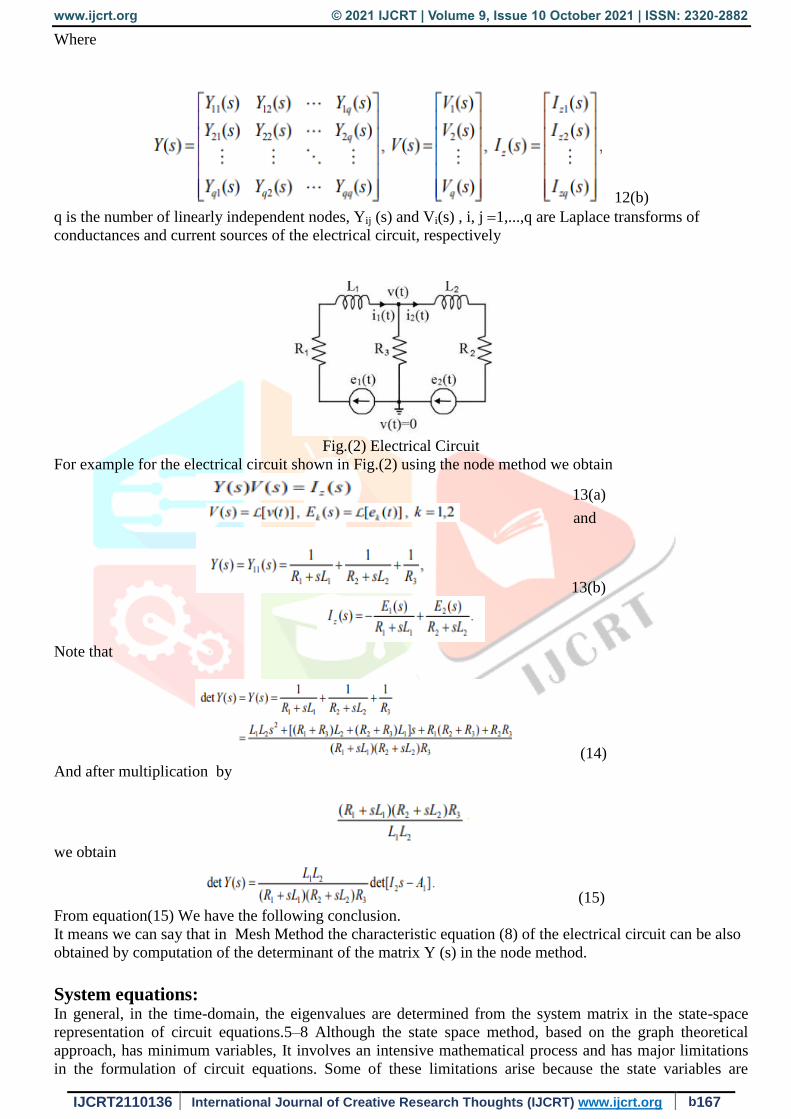
Fig.(2) Electrical Circuit

For example for the electrical circuit shown in Fig.(2) using the node method we obtain

13(a)

and

13(b)

Note that

(14)

And after multiplication by

we obtain

(15)

From equation(15) We have the following conclusion.

It means we can say that in Mesh Method the characteristic equation (8) of the electrical circuit can be also

obtained by computation of the determinant of the matrix Y (s) in the node method.

System equations: In general, in the time-domain, the eigenvalues are determined from the system matrix in the state-space

representation of circuit equations.5–8 Although the state space method, based on the graph theoretical

approach, has minimum variables, It involves an intensive mathematical process and has major limitations

in the formulation of circuit equations. Some of these limitations arise because the state variables are



capacitor voltages and inductor currents. Not every circuit element can be easily included into the state

equations. It has a structure of differential equations. Especially, there are some restrictions in the analysis

of active circuits. Therefore, students of electrical engineering generally have these difficulties in obtaining

the state-space representation of system equations. It is not always suitable to use this method for obtaining

both eigenvalues and transfer functions. In this study, it is shown that the eigenvalues can be easily

determined according to nodal and mesh equations in the s-domain, through more efficient and

understandable analysis methods in circuit analysis courses. It has a structure of algebraical equations. There

are no restrictions in the formulation of circuit equations. In this paper the nodal and mesh analysis methods

with virtual sources for some special cases in circuit analysis are used.

The system equations in the algebraical structure, in the Laplace domain, obtained by using nodal or mesh

analysis method, relating to a linear circuit are

AX(s)= BU(s) (1) Where, A, B are coefficient matrices, U(s) is the source vector, X(s) is the unknown vector. The frequency-

dependent elements (inductor, capacitor) can be entered in the form having

s(sL, sC) or 1/s(1/sL, 1/sC) into the system equations. Matrix A is also called the characteristic matrix. By

taking the inverse of matrix A, solutions of the system equations are given as in equation(2), as follows

(2) where det(A) denotes the determinant of matrix A, and adj are notes the adjoint matrix. It is obvious that

solutions of equation(2) are fractional. The determinant of the characteristic matrix (A) has also fractional

and polynomial form as in equation(3). Q(s) represents the numerator of the determinant and R(s) represents

the denominator of the determinant.

(3)

The determinant expression in equation (3) is substituted into equation (2)

(4) According to Equation(4), all variables relating to any circuit have the same denominator, Q(s). It is the

numerator of determinant of the coefficient matrix (A) in equation (3).

Therefore, Q(s) polynomial is also called the characteristic equation. The eigenvalues, indirectly poles, of

any circuit are obtained from the roots of the characteristic polynomial, Q(s) = 0. In the proposed approach,

the system equations in the form of equation(1) are obtained algebraically by nodal or mesh analysis in the

Laplace (s) domain. The characteristic equation, Q(s), is determined in terms of the numerator of

determinant of the coefficient matrix (A) relating to system equations. Later, the eigenvalues of the circuit

are easily obtained from the roots of the characteristic equation.

Applications: Example 1. Consider the circuit shown in Fig.(1). Element values are R = 2 Ω, C1 = C2 = 3 F, L = 5 H.

Mesh equations in the s-domain are as follows. The variables of the method are I1, I2 mesh currents.



Let’s rearrange the system equations in matrix form.

(5)

After substituting the element values into the system equations, the determinant of the

coefficient matrix (A) is obtained as follows.

Fig.(1) Circuit for example 1

(6)

After solving the system equations in (5), the circuit variables, mesh currents, are obtained as follows.

(7) It can be easily seen that all variables relating to the circuit have the same denominator, the characteristic

equation (Q(s)). The roots of characteristic equation (Q(s)) give the eigenvalues of the third order circuit: α1

≅ −0.0394 + 0.3534i, α2 ≅ −0.0394 − 0.3534i, α3 = −0.0879. The circuit is stable because all eigenvalues

are located on the left-hand side of the complex

s-plane.

Conclusion: The difficulty of determining the eigenvalues in circuit analysis courses depends on obtaining the system

equations. In general, the eigenvalues are determined from a state variables method having a structure of

differential equations and some restrictions in obtaining the system equations. In this paper, it is shown how

the eigenvalues of linear circuits can be determined according to the characteristic equation created by nodal

and mesh analysis, in algebraical form. In terms of complexity, the proposed method is simpler and more

understandable than the commonly used form of state equations. The method is general and can be easily

applied to all possible active and passive circuits. It has no restrictions. The main advantages of the method

are efficient, systematic, and understandable in terms of advances in student learning. Students can easily

determine the eigenvalues and, moreover, can write a computer program about computation of the

eigenvalues by employing the presented method and also the problem of calculation of the characteristic

equations of the standard positive and linear electrical circuits has been addressed.



Acknowledgement: First and foremost, I would like to thank God, the almighty for his blessings I would like to thank my wife

Sarita Srivastava for standing besides me throughout my career while writing this paper. Also I would like

to thank my sons Er.Satyam Srivastava and Dr.Kumar Yash Srivastava and my daughter Dr.Shriya

Srivastava.

References

[1] Antsaklis P.J., Michel A.N.: Linear Systems. Birkhauser, Boston, 2006.

[2] Cholewicki T.: Theoretical Electrotechnics, WNT, Warszawa, 1967 (in Polish).

[3] Farina L., Rinaldi S.: Positive Linear Systems; Theory and Applications. J. Wiley, New York, 2000. [4]

Kaczorek T.: A class of positive and stable time-varying electrical circuits. Electrical Review, vol. 91, no. 5,

2015, 121-124.

[5] Kaczorek T.: Constructability and observability of standard and positive electrical circuits. Electrical

Review, vol. 89, no. 7, 2013, 132-136.

[6] Kaczorek T.: Decoupling zeros of positive continuous-time linear systems and electrical circuits.

Advances in Systems Science. Advances in Intelligent Systems and Computing, vol. 240, 2014, Springer, 1-

15.

[7] Kaczorek T.: Minimal-phase positive electrical circuits. Electrical Review, vol. 92, no. 3, 2016, 182-189.

[8] Kaczorek T.: Normal positive electrical circuits. IET Circuits Theory and Applications, vol. 9, no. 5,

2015, 691-699.

[9] Kaczorek T.: Positive 1D and 2D Systems. Springer-Verlag, London, 2002.

[10] Kaczorek T.: Positive electrical circuits and their reachability. Archives of Electrical Engineering, vol.

60, no. 3, 2011, 283-301.

[11] Kaczorek T.: Positive fractional linear electrical circuits. Proceedings of SPIE, vol. 8903, Bellingham

WA, USA, Art. No 3903-35.

[12] Kaczorek T.: Positive linear systems with different fractional orders. Bull. Pol. Acad. Sci. Techn., vol.

58, no. 3, 2010, 453-458.

[13] Kaczorek T.: Positive systems consisting of n subsystems with different fractional orders. IEEE Trans.

Circuits and Systems – regular paper, vol. 58, no. 6, June 2011, 1203-1210.

[14] Kaczorek T.: Positive unstable electrical circuits. Electrical Review, vol. 88, no. 5a, 2012, 187-192.

[15] Kaczorek T.: Zeroing of state variables in descriptor electrical circuits by statefeedbacks. Electrical

Review, vol. 89, no. 10, 2013, 200-203.

[16] Kaczorek T., Rogowski K.: Fractional Linear Systems and Electrical Circuits. Studies in Systems,

Decision and Control, vol. 13, Springer, 2015.

[17] Kailath T.: Linear Systems. Prentice-Hall, Englewood Cliffs, New York, 1980.

BIBLIOGRAPHY

Dr. Shailendra Kumar Srivastava is a popular name amongst the science enthusiasts.

He is currently serving as the Principal of the prestigious Mahatma Gandhi Post

Graduate College(Gorakhpur, Uttar Pradesh) for the past 7 years.

He has also worked as Assistant Professor for 8 years and as Associate Professor for

20 years in the past.

Dr. Subhash Kumar Sharma, Assistant Professor, Department of Electronics,

Mahatma Gandhi Post Graduate College ,Gorakhpur working as assistant Professor

since 2012 to till date.

He has also worked as Assistant Professor from 2005 to 2011 in Department Of

Electronics , DDU Gorakhpur University, Gorakhpur.

Evaluation of Eigenvalues of Linear Electrical Circuits ...

Documents

Transcript of Evaluation of Eigenvalues of Linear Electrical Circuits ...