Evaluation of DEGADIS 2.1 Using Advisory Bulletin ADB-10-07
109
Evaluation of DEGADIS 2.1 Using Advisory Bulletin ADB-10-07 Cooperating Agency: U.S. Department of Transportation, Pipeline and Hazardous Materials Safety Administration Washington, DC 20426 Federal Energy Re gulatory Co mmission Office of Energy Projects July 2011
Transcript of Evaluation of DEGADIS 2.1 Using Advisory Bulletin ADB-10-07

Evaluation of DEGADIS 2.1 Using Advisory Bulletin ADB-10-07
Cooperating Agency:
U.S. Department of Transportation, Pipeline and Hazardous Materials Safety Administration
Washington, DC 20426
Fede
ral E
nerg
y
Regu
lato
ryCo
mm
issi
on Office of Energy Projects
July 2011

EVALUATION OF DEGADIS 2.1
USING ADVISORY BULLETIN ADB-10-07
TABLE OF CONTENTS Page
1.0 Introduction .........................................................................................................................1
1.1 Background...................................................................................................................1
1.1.1 Model Evaluation Protocol.....................................................................................1
1.1.2 PHMSA Advisory Bulletin ADB-10-07 ................................................................2
1.2 Project Scope ................................................................................................................3
2.0 Results of the 2007 Partial DEGADIS Evaluation..............................................................4
2.1 Scientific Assessment and Verification ........................................................................4
2.2 Application of the Full Validation Database to DEGADIS..........................................4
2.2.1 Validation Cases Modeled (MER Section 6.2.1) ...................................................4
2.2.2 Model Performance for Key Statistical Evaluation Parameters (MER Section 6.2.2)..........................................................................................................5
2.2.3 Evaluation Against Quantitative Assessment Criteria (MER Section 6.2.3) .........6
2.2.4 Additional Comments (MER Section 6.2.4) ..........................................................7
3.0 Application of PHMSA Advisory Bulletin ADB-10-07 ...................................................17
3.1 Source Geometry Handled by the Dispersion Model (MER Section 2.1.1.2; ADB-10-07 Section 1.a-d).............................................................................17
3.2 Wind Field (MER Section 2.2.2.1; ADB-10-07 Section 2) ........................................17
3.3 Stratification (MER Section 2.2.2.3; ADB-10-07 Section 3) .....................................17
3.4 Terrain Types Available (MER section 2.2.3.1; ADB-10-07 Section 4) & Complex Effects (MER section 2.3.1.2; ADB-10-07 Section 4)................................18
3.5 Obstacle Types Available (MER Section 2.2.4.1; ADB-10-07 Section 5) & Complex Effects (MER Section 2.4.3.1; ADB-10-07 Section 5)...............................................18
3.6 Turbulence Modeling (MER Section 2.3.1.5; ADB-10-07 Section 6) .......................18
3.7 Boundary Conditions (MER Section 2.3.1.7; ADB-10-07 Section 7)........................19
3.8 Complex Effects: Aerosols (MER Section 2.3.1.1; ADB-10-07 Section 8)...............19
3.9 Computational Mesh (MER Section 2.4.3.1; ADB-10-07 Section 9).........................20
3.10 Discretization Methods (MER Section 2.4.2.3; ADB-10-07 Section 10)...................20
3.11 Sources of Model Uncertainty (MER Section 2.6; ADB-10-07, Section 11).............20
3.12 Sensitivity to Input (MER Section 2.6.4; ADB-10-07 Section 12).............................20
3.13 Limits of Applicability (MER Section 2.7; ADB-10-07 Section 13) .........................22
EVALUATION OF DEGADIS 2.1
USING ADVISORY BULLETIN ADB-10-07
TABLE OF CONTENTS (cont’d) Page
ii
3.14 Evaluation Against the MEP Quantitative Assessment Criteria (MER Section 6.2.4; ADB-10-07 Section 14) .......................................................................23
3.14.1 Uncertainty Analysis of Model Input ...................................................................23
3.14.2 Uncertainty Analysis of Model Output ................................................................38
3.14.3 Uncertainty Analysis of Experimental Data.........................................................42
3.14.4 Uncertainty Analysis Results ...............................................................................46
3.14.5 Additional Specific Performance Measures .........................................................46
3.14.6 Individual Specific Performance Measures..........................................................46
3.14.7 Model Input/Output Results .................................................................................46
3.14.8 Specific Performance Measures Results ..............................................................47
3.14.9 Input and Output Files..........................................................................................47
4.0 Conclusions .......................................................................................................................48
4.1 Scientific Assessment .................................................................................................48
4.2 Verification .................................................................................................................50
4.3 Validation....................................................................................................................51
4.4 Sensitivity Analyses....................................................................................................54
4.5 Model Suitability and Limitations ..............................................................................55
APPENDIX A SENSITIVITY CASE RESULTS
APPENDIX B REFERENCES
APPENDIX C LIST OF PREPARERS

EVALUATION OF DEGADIS 2.1
USING ADVISORY BULLETIN ADB-10-07
TABLE OF CONTENTS (cont’d) Page
iii
LIST OF TABLES
2.2-1 SPM Evaluation against Quantitative Assessment Criteria: Overall Trial Average.........................................................................................................................6
2.2-2 SPM Evaluation against Quantitative Assessment Criteria: Individual Trial Average................................................................................................................... 8-11
3.12-1 Sensitivity Case Designations.....................................................................................21
3.14-1 Pool Diameters as a Function of Vaporization Rate ...................................................24
3.14-2 Distance to LFL Uncertainty Due to Pool Spread Velocity and Vaporization Rate .............................................................................................................................25
3.14-3 Distance to LFL Uncertainty Due To Surface Roughness Length: Maplin Sands...........................................................................................................................28
3.14-4 Distance to LFL Uncertainty Due To Surface Roughness Length: Burro & Coyote ..........................................................................................................29
3.14-5 Concentration Uncertainty Due To Surface Roughness Length: Thorney Island.......30
3.14-6 Sensitivity Case Inputs................................................................................................33
3.14-7 Sensitivity of the Water Transfer Sub-Model .............................................................34
3.14-8 Effect of Time-Average on the Maximum Arc-wise Concentration .................... 35-36
3.14-9 Effect of Time-Average on the Plume Width .............................................................37
3.14-10 Comparison of Interpolation / Extrapolation Methodologies: Experiment Results.........................................................................................................................39
3.14-11 Comparison of Interpolation / Extrapolation Methodologies: Model Results ............40
3.14-12 Experimental and Model Results for Lower Flammability Limits .............................41
3.14-13 Interpolation and Extrapolation of the Experimental and Model Results...................41
3.14-14 Uncertainty in the Sensor Measurement of Gas Concentration ............................ 43-45
EVALUATION OF DEGADIS 2.1
USING ADVISORY BULLETIN ADB-10-07
TABLE OF CONTENTS (cont’d) Page
iv
LIST OF FIGURES
2.2-1 Short Time Average Measured and Predicted Concentrations ...................................13
2.2-2 Long Time Average Measured and Predicted Concentrations ...................................13
2.2-3 Short Time Average Measured and Predicted Distance to LFL .................................15
2.2-4 Short Time Average MG and VG...............................................................................16
2.2-5 Long Time Average MG and VG ...............................................................................16
4.3-1 Predicted Concentration against Measured Concentration .........................................52

ACRONYMS & ABBREVIATIONS
v
ABS American Bureau of Shipping
Advisory Bulletin Pipeline and Hazardous Materials Safety Administration Advisory Bulletin ADB-10-07
cm centimeter
C.F.R. Code of Federal Regulations
CSF concentration safety factor
CSF_LFL concentration safety factor at the lower flammability limit
DSF distance safety factor
DSF_LFL distance safety factor to the lower flammability limit
FAC2 factor of 2
FERC or Commission Federal Energy Regulatory Commission
FPRF Fire Protection Research Foundation
km kilometer
LFL lower flammability limit
LNG liquefied natural gas
m meter
m/s meters per second
MDA Modeler’s Data Archive
MEP Model Evaluation Protocol
MER Model Evaluation Report
MG geometric mean bias
MRB mean relative bias
MRSE mean relative square error
NASFM National Association of State Fire Marshals
NFPA National Fire Protection Association
PHMSA Pipelines and Hazardous Materials Safety Administration of the U.S. Department of Transportation
SPM statistical performance measure
VG geometric variance

1.0 INTRODUCTION
1.1 BACKGROUND
In the United States, Title 49, Code of Federal Regulations (C.F.R.), Part 193 prescribes the federal safety standards for liquefied natural gas (LNG) facilities. The siting requirements in Subpart B specify that each LNG container and LNG transfer system must have vapor-gas dispersion exclusion zones calculated in accordance with §193.2059. The regulation specifically approves the use of two models for performing these calculations, DEGADIS and FEM3A, but also allows the use of alternative models approved by the U.S. Department of Transportation.
The integral model DEGADIS was developed for the Gas Research Institute and the U.S. Coast Guard specifically to account for effects such as gravity spreading, negative or positive buoyancy effects on air entrainment, surface to cloud heat transfer, and phase change energy effects associated with air humidity in modeling dispersion of dense gases. The theoretical and experimental basis for the model was described in Gas Research Institute Report No. 89/0242, LNG Vapor Dispersion Prediction with the DEGADIS Dense Gas Dispersion Model. Extensive vapor dispersion experimental and analytical work, beginning in 1982, was also conducted prior to adoption of DEGADIS into the federal regulations in 1997 (RSPA, 1997).
1.1.1 Model Evaluation Protocol
In 2006, the Fire Protection Research Foundation (FPRF), at the request of the National Fire Protection Association (NFPA), began to develop guidance to be used in assessing vapor dispersion models in analyzing LNG facilities. The main focus of this effort was to develop a means to review dispersion models based on their scientific basis and through comparison with experimental data. The result of this study, released in 2007, was a Model Evaluation Protocol (MEP) that could be applied to determine the suitability of any dispersion model to simulate dispersion of LNG spills on land (Ivings et al., 2007). In 2009, the NFPA LNG Technical Committee revised the 2009 edition of NFPA 59A, Standard for the Production, Storage, and Handling of Liquefied Natural Gas, to remove the prescription of DEGADIS and require that a model be acceptable to the Authority Having Jurisdiction based on an evaluation using the MEP.
The MEP is based on the European Union Scientific Model Evaluation of Dense Gas Dispersion Models, known as the SMEDIS protocol, which is in turn based on criteria set by the Council of European Communities Model Evaluation Group on Heavy Gas Dispersion. The MEP consists of three stages: scientific assessment; verification; and validation. Initially, the physical, mathematical and numerical basis of the model is reviewed (i.e., scientific assessment). Then, the model developer provides evidence demonstrating that the model correctly implements the bases identified during scientific assessment (i.e. verification). Finally, various simulations are performed with the model

2
and compared to a database of experimental results from wind tunnel and field trial tests (i.e. validation) (Ivings et al., 2007).
Results of the scientific assessment, model verification, and validation are contained in the Model Evaluation Report (MER). Ivings et al. (2007) specifies that the MER is composed of eight sections:
Section 0. Evaluation information; Section 1. General model description; Section 2. Scientific basis of model; Section 3. User-orientated basis of model; Section 4. Verification performed; Section 5. Evaluation against MEP qualitative assessment criteria; Section 6. Validation performed and evaluation against MEP quantitative
assessment criteria; and Section 7. Conclusions
The results of application of the MEP to a specific model, as summarized in these seven sections of the MER, can then be used as a basis for establishing the limitations and safety margins of the dispersion model.
As part of the protocol development, the MEP was partly applied to both DEGADIS and FEM3A. Based on the scientific assessment and model verification, the limits of applicability of both models were described and an assessment of previous validations were given. However, the lack of a standard validation database prevented application of the full MEP from being within the scope of that report (Ivings et al., 2007). In February 2009, the FPRF completed and released both the validation database and the “Guide to the LNG Model Validation Database,” with subsequent revisions in September 2009 and May 2010 (Coldrick et al., 2010). Validation of DEGADIS or FEM3A against the database was not performed as application of the remaining portions of the MEP was not within the scope of that effort.
1.1.2 PHMSA Advisory Bulletin ADB-10-07
In 2009, the National Association of State Fire Marshals (NASFM) released an independent review of the MEP. The goal of NASFM’s report, “Final Report: Review of the LNG Vapor Dispersion Model Evaluation Protocol,” was to ensure that hazard models evaluated with the MEP process were suitable for the specific situations in which LNG facilities were being planned (AcuTech, 2009). The panelists for the NASFM effort suggested improvements to the MEP and also identified difficulties in using this approach in a regulatory setting.

3
After reviewing the MEP report and validation database issued by the FPRF in 2007 and 2010, as well as the NASFM study, the U.S. Department of Transportation’s Pipelines and Hazardous Materials Safety Administration (PHMSA) issued Advisory Bulletin ADB-10-07 (Advisory Bulletin) to provide guidance on obtaining approval of alternative vapor-gas dispersion models under Subpart B of 49 C.F.R. Part 193 (PHMSA, 2010). The approach is based on the scientific assessment, verification, and validation of the MEP with adjustments to address the concerns raised by NASFM, as well as by staff of the Federal Energy Regulatory Commission (FERC or Commission).
1.2 PROJECT SCOPE
This document provides the complete MEP, as adjusted by modifications from the PHMSA Advisory Bulletin, to the DEGADIS dense gas vapor dispersion model specified in 49 C.F.R. § 193.2059. This serves two purposes: (1) completing the MEP for DEGADIS partially done by Ivings et al. (2007); and (2) illustrating the appropriate level of information requested by the Advisory Bulletin for obtaining PHMSA approval of an alternative vapor-gas dispersion model as allowed by §193.2059(a).
The document is intended for developers/evaluators who are going to submit a request to PHMSA for an alternative model approval under 49 C.F.R. § 193.2059(a). Sections 2.0 and 3.0, as well as the validation database, provide an example of the level of detail requested by ABD-10-7. Section 4.0 provides an example of the suitability and limitation descriptions which would be included in a public PHMSA approval.
Completion of the MEP and the DEGADIS validation work was performed by FERC staff. The validation work which accompanies this report is included in the Excel spreadsheet, entitled “DEGADIS Validation Database.xls,” being issued concurrently with this document. Review of the MEP results and limitations for the suitable use of the DEGADIS model in exclusion zone calculations was done by staff of the PHMSA.
4
2.0 RESULTS OF THE 2007 PARTIAL DEGADIS EVALUATION
2.1 SCIENTIFIC ASSESSMENT AND VERIFICATION
Appendix B 10.2 of Ivings et al., (2007) addressed all of the sections of the MEP guidance, except for Section 6.2, “Evaluation against MEP quantitative assessment criteria.” The conclusions of Appendix B are available upon request from the FPRF and are not repeated in this document. Certain sections of the scientific assessment that were addressed did not provide enough detail to thoroughly evaluate the limitations of the model. As discussed in the following sections, the Advisory Bulletin was used to address those areas.
2.2 APPLICATION OF THE VALIDATION DATABASE TO DEGADIS
Using the LNG Model Validation Database, the following sections of the MEP can now be completed for the DEGADIS model (Coldrick et al., 2010):
6.2.1 Validation cases modeled; 6.2.2 Model performance for key statistical evaluation parameters; 6.2.3 Evaluation against quantitative assessment criteria; and 6.2.4 Additional comments.
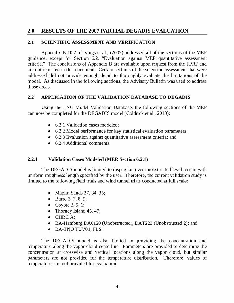
2.2.1 Validation Cases Modeled (MER Section 6.2.1)
The DEGADIS model is limited to dispersion over unobstructed level terrain with uniform roughness length specified by the user. Therefore, the current validation study is limited to the following field trials and wind tunnel trials conducted at full scale:
Maplin Sands 27, 34, 35; Burro 3, 7, 8, 9; Coyote 3, 5, 6; Thorney Island 45, 47; CHRC A; BA-Hamburg DA0120 (Unobstructed), DAT223 (Unobstructed 2); and BA-TNO TUV01, FLS.
The DEGADIS model is also limited to providing the concentration and
temperature along the vapor cloud centerline. Parameters are provided to determine the concentration at crosswise and vertical locations along the vapor cloud, but similar parameters are not provided for the temperature distribution. Therefore, values of temperatures are not provided for evaluation.

5
2.2.2 Model Performance for Key Statistical Evaluation Parameters (MER Section 6.2.2)
The model results are compared to the experimental measurements to develop the following statistical performance measure (SPM) values: mean relative bias (MRB); geometric mean bias (MG); mean relative square error (MRSE); geometric variance (VG); factor of 2 (FAC2); concentration safety factor (CSF); concentration safety factor at the lower flammability limit (CSF_LFL); distance safety factor (DSF); and distance safety factor at the lower flammability limit (DSF_LFL). The SPM values are shown in Table 2.2-1. Shaded cells indicated where the SPM were not within the MEP acceptance criteria.
Table 2.2-1:
SPM Evaluation against Quantitative Assessment Criteria: Overall Trial Average Quantitative Criteria
Data Set
-0.4
<M
RB
<0.
4
0.67
< M
G<
1.5
MR
SE
<2.
3
VG
<3.
3
FA
C2
>50
%
0.5<
CS
F<
2
0.5<
CS
F_L
FL
<2
0.5<
DS
F<
2
0.5<
DS
F_L
FL
<2
Maximum Arc-wise Gas Concentration Field Trials (Short Time Avg.)
-0.47 0.60 0.49 1.80 58% 1.93 1.80 N/A N/A
Field Trials (Long Time Avg.)
-0.77 0.41 0.92 3.76 36% 3.13 N/A N/A N/A
Wind-Tunnel Tests (Scaled)
0.79 2.43 0.80 2.84 36% 0.47 N/A N/A N/A
Maximum Gas Concentration Arc-wise Distance Field Trials (Short Time Avg.)
-0.32 0.72 0.21 1.25 89% N/A N/A 1.47 1.43
Field Trials (Long Time Avg.)
-0.29 0.74 0.19 1.23 89% N/A N/A 1.43 N/A
Wind-Tunnel Tests (Scaled)
0.50 1.68 0.32 1.42 68% N/A N/A 0.62 N/A
6
Table 2.2-1 (cont’d):
SPM Evaluation against Quantitative Assessment Criteria: Overall Trial Average Quantitative Criteria
Data Set
-0.4
<M
RB
<0.
4
0.67
< M
G<
1.5
MR
SE
<2.
3
VG
<3.
3
FA
C2
>50
%
0.5<
CS
F<
2
0.5<
CS
F_L
FL
<2
0.5<
DS
F<
2
0.5<
DS
F_L
FL
<2
Maximum Point-wise Gas Concentration Field Trials (Short Time Avg.)
0.52 3.73 1.28 >1,000 46% 0.91 N/A N/A N/A
Field Trials (Long Time Avg.)
-0.12 1.28 1.26 >1,000 33% 2.70 N/A N/A N/A
Wind-Tunnel Tests (Scaled)
0.24 1.50 0.48 11.92 69% 1.07 N/A N/A N/A
Cloud Width Field Trials (Short Time Avg.)
0.46 1.61 0.28 1.35 84% N/A N/A 0.64 N/A
Field Trials (Long Time Avg.)
0.24 1.28 0.12 1.14 92% N/A N/A 0.81 N/A
Wind-Tunnel Tests (Scaled)
-0.09 0.91 0.03 1.03 100% N/A N/A 1.11 N/A
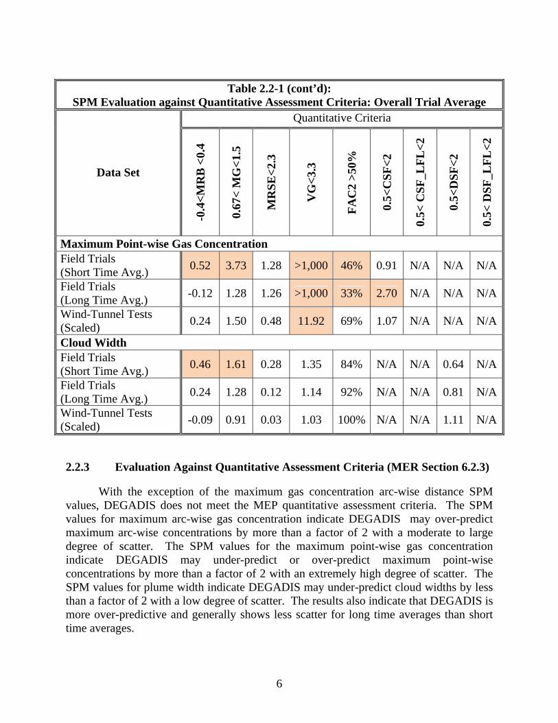
2.2.3 Evaluation Against Quantitative Assessment Criteria (MER Section 6.2.3)
With the exception of the maximum gas concentration arc-wise distance SPM values, DEGADIS does not meet the MEP quantitative assessment criteria. The SPM values for maximum arc-wise gas concentration indicate DEGADIS may over-predict maximum arc-wise concentrations by more than a factor of 2 with a moderate to large degree of scatter. The SPM values for the maximum point-wise gas concentration indicate DEGADIS may under-predict or over-predict maximum point-wise concentrations by more than a factor of 2 with an extremely high degree of scatter. The SPM values for plume width indicate DEGADIS may under-predict cloud widths by less than a factor of 2 with a low degree of scatter. The results also indicate that DEGADIS is more over-predictive and generally shows less scatter for long time averages than short time averages.
7
2.2.4 Additional Comments (MER Section 6.2.4)
As stated in the Advisory Bulletin, model predictions outside the quantitative assessment criteria do not necessarily mean that the model is unacceptable. However, such results may alternatively impact the safety factor associated with the model.
Based on the MEP groups, it would appear that DEGADIS is generally over-predictive by more than a factor of 2 and therefore additional safety margins may be seen as over-burdensome. However, upon examination of individual test and sensor data, SPM trends become clearer in the model predictions, as shown in Table 2.2-2. Results of the individual tests and sensor data trends are discussed below.

8
Table 2.2-2:
SPM Evaluation against Quantitative Assessment Criteria: Individual Trial Average Quantitative Criteria
Data Set
-0.4
<M
RB
<0.
4
0.67
< M
G<
1.5
MR
SE
<2.
3
VG
<3.
3
FA
C2
>50
%
0.5<
CS
F<
2
0.5<
CS
F_L
FL
<2
0.5<
DS
F<
2
0.5<
DS
F_L
FL
<2
Maximum Arc-Wise Gas Concentration Maplin Sands 27 (short) -0.08 0.93 0.37 1.55 75% 1.29 1.40 N/A N/AMaplin Sands 34 (short) 0.24 1.28 0.06 1.06 100% 0.78 0.74 N/A N/AMaplin Sands 35 (short) -0.33 0.71 0.17 1.20 83% 1.45 1.28 N/A N/ABurro 3 (short) -1.00 0.32 1.05 2.48 0% 3.31 3.37 N/A N/ABurro 3 (long) -1.37 0.18 1.90 21.49 0% 5.92 N/A N/A N/ABurro 7 (short) -0.79 0.42 0.78 2.64 33% 2.62 1.86 N/A N/ABurro 7 (long) -1.09 0.28 1.26 5.61 0% 3.75 N/A N/A N/ABurro 8 (short) 0.08 1.09 0.21 1.25 75% 1.01 0.77 N/A N/ABurro 8 (long) -0.09 0.90 0.36 1.50 50% 1.35 N/A N/A N/ABurro 9 (short) -0.64 0.51 0.46 1.70 67% 2.04 1.95 N/A N/ABurro 9 (long) -0.80 0.41 0.80 2.89 33% 2.78 N/A N/A N/ACoyote 3 (short) -0.93 0.36 0.91 3.36 0% 2.88 2.78 N/A N/ACoyote 3 (long) -1.42 0.17 2.02 25.27 0% 6.30 N/A N/A N/ACoyote 5 (short) -0.57 0.56 0.33 1.44 75% 1.80 1.77 N/A N/ACoyote 5 (long) -1.17 0.26 1.40 9.10 0% 4.05 N/A N/A N/ACoyote 6 (short) -0.68 0.49 0.50 1.48 75% 2.10 2.06 N/A N/ACoyote 6 (long) -1.03 0.32 1.08 3.69 0% 3.21 N/A N/A N/AThorney Island 45 (long) -0.29 0.74 0.20 1.24 89% 1.42 N/A N/A N/AThorney Island 47 (long) -0.28 0.75 0.18 1.21 83% 1.42 N/A N/A N/ACHRC A (scaled) 0.31 1.36 0.10 1.11 100% 0.74 N/A N/A N/AHamburg DA0120 (scaled) 1.15 3.81 1.37 6.56 13% 0.28 N/A N/A N/AHamburg DAT 223 (scaled) 0.63 1.97 0.56 1.95 33% 0.56 N/A N/A N/ATNO FLS (scaled) 0.81 2.42 0.75 2.46 17% 0.44 N/A N/A N/A

9
Table 2.2-2 (cont’d):
SPM Evaluation against Quantitative Assessment Criteria: Individual Trial Average Quantitative Criteria
Data Set
-0.4
<M
RB
<0.
4
0.67
< M
G<
1.5
MR
SE
<2.
3
VG
<3.
3
FA
C2
>50
%
0.5<
CS
F<
2
0.5<
CS
F_L
FL
<2
0.5<
DS
F<
2
0.5<
DS
F_L
FL
<2
Maximum Gas Concentration Arc-Wise Distance Maplin Sands 27 (short) -0.08 0.92 0.10 1.11 100% N/A N/A 1.13 1.20Maplin Sands 34 (short) 0.16 1.18 0.03 1.03 100% N/A N/A 0.85 0.80Maplin Sands 35 (short) -0.26 0.77 0.11 1.12 100% N/A N/A 1.33 1.19Burro 3 (short) -0.63 0.52 0.43 1.60 50% N/A N/A 1.96 2.21Burro 3 (long) -0.55 0.56 0.35 1.47 75% N/A N/A 1.82 N/ABurro 7 (short) -0.65 0.50 0.56 1.93 33% N/A N/A 2.18 1.52Burro 7 (long) -0.64 0.50 0.56 1.93 33% N/A N/A 2.17 N/ABurro 8 (short) 0.05 1.05 0.10 1.11 100% N/A N/A 1.00 0.87Burro 8 (long) 0.04 1.04 0.11 1.11 100% N/A N/A 1.02 N/ABurro 9 (short) -0.41 0.66 0.22 1.27 67% N/A N/A 1.57 1.54Burro 9 (long) -0.36 0.69 0.21 1.25 67% N/A N/A 1.52 N/ACoyote 3 (short) -0.55 0.57 0.31 1.39 100% N/A N/A 1.77 1.78Coyote 3 (long) -0.48 0.61 0.24 1.29 100% N/A N/A 1.65 N/ACoyote 5 (short) -0.36 0.70 0.13 1.15 100% N/A N/A 1.44 1.48Coyote 5 (long) -0.14 0.87 0.05 1.05 100% N/A N/A 1.17 N/ACoyote 6 (short) -0.48 0.62 0.23 1.27 100% N/A N/A 1.63 1.67Coyote 6 (long) -0.45 0.63 0.20 1.23 100% N/A N/A 1.58 N/AThorney Island 45 (long) -0.06 0.94 0.08 1.09 100% N/A N/A 1.10 N/AThorney Island 47 (long) -0.28 0.74 0.18 1.23 83% N/A N/A 1.44 N/ACHRC A (scaled) 0.24 1.27 0.07 1.07 100% N/A N/A 0.79 N/AHamburg DA0120 (scaled) 0.73 2.17 0.57 1.90 25% N/A N/A 0.47 N/AHamburg DAT 223 (scaled) 0.36 1.45 0.19 1.22 100% N/A N/A 0.71 N/ATNO FLS (scaled) 0.46 1.61 0.26 1.31 83% N/A N/A 0.64 N/A

10
Table 2.2-2 (cont’d):
SPM Evaluation against Quantitative Assessment Criteria: Individual Trial Average Quantitative Criteria
Data Set
-0.4
<M
RB
<0.
4
0.67
< M
G<
1.5
MR
SE
<2.
3
VG
<3.
3
FA
C2
>50
%
0.5<
CS
F<
2
0.5<
CS
F_L
FL
<2
0.5<
DS
F<
2
0.5<
DS
F_L
FL
<2
Maximum Point-Wise Gas Concentration Burro 3 (short) 1.04 16.28 1.95 >1000 45% 0.47 N/A N/A N/ABurro 3 (long) 0.49 3.87 1.38 >1000 27% 0.97 N/A N/A N/ABurro 7 (short) 0.42 2.78 1.20 >100 60% 0.96 N/A N/A N/ABurro 7 (long) -0.24 0.89 1.67 31.6 10% 3.05 N/A N/A N/ABurro 8 (short) 0.41 4.05 1.10 >1000 52% 0.98 N/A N/A N/ABurro 8 (long) 0.25 4.10 1.19 >1000 52% 1.25 N/A N/A N/ABurro 9 (short) 0.38 3.02 1.01 >1000 60% 0.96 N/A N/A N/ABurro 9 (long) -0.03 1.34 0.91 33.6 40% 1.52 N/A N/A N/ACoyote 3 (short) 0.80 4.05 1.58 >100 42% 0.65 N/A N/A N/ACoyote 3 (long) -0.77 0.30 1.73 42.9 25% 8.06 N/A N/A N/ACoyote 5 (short) 0.60 2.93 1.31 >100 29% 0.92 N/A N/A N/ACoyote 5 (long) -0.24 0.77 0.93 5.21 43% 2.44 N/A N/A N/ACoyote 6 (short) 0.13 1.66 0.98 59.0 38% 1.31 N/A N/A N/ACoyote 6 (long) -0.49 0.64 1.16 8.14 15% 2.51 N/A N/A N/ACHRC A (scaled) 0.14 1.61 0.58 >100 78% 1.30 N/A N/A N/AHamburg DAT 223 (scaled) 0.51 1.72 0.37 1.53 63% 0.62 N/A N/A N/ABA TNO TUV01 (scaled) -0.08 0.92 0.21 1.25 100% 1.20 N/A N/A N/ABA TNO FLS (scaled) 0.42 1.59 0.47 1.80 52% 0.76 N/A N/A N/A
11
Table 2.2-2 (cont’d): SPM Evaluation against Quantitative Assessment Criteria: Individual Trial Average
Quantitative Criteria
Data Set
-0.4
<M
RB
<0.
4
0.67
< M
G<
1.5
MR
SE
<2.
3
VG
<3.
3
FA
C2
>50
%
0.5<
CS
F<
2
0.5<
CS
F_L
FL
<2
0.5<
DS
F<
2
0.5<
DS
F_L
FL
<2
Cloud Width Burro 3 (short) 0.78 2.30 0.65 2.11 33% N/A N/A 0.45 N/ABurro 3 (long) 0.51 1.69 0.28 1.35 67% N/A N/A 0.60 N/ABurro 7 (short) 0.43 1.55 0.20 1.24 100% N/A N/A 0.65 N/ABurro 7 (long) 0.25 1.28 0.07 1.07 100% N/A N/A 0.78 N/ABurro 8 (short) 0.34 1.42 0.21 1.25 75% N/A N/A 0.74 N/ABurro 8 (long) 0.38 1.48 0.22 1.27 75% N/A N/A 0.71 N/ABurro 9 (short) 0.49 1.65 0.25 1.31 100% N/A N/A 0.61 N/ABurro 9 (long) 0.24 1.27 0.06 1.06 100% N/A N/A 0.79 N/ACoyote 3 (short) 0.59 1.85 0.39 1.55 67% N/A N/A 0.56 N/ACoyote 3 (long) -0.18 0.83 0.08 1.08 100% N/A N/A 1.23 N/ACoyote 5 (short) 0.49 1.65 0.22 1.29 100% N/A N/A 0.61 N/ACoyote 5 (long) 0.34 1.41 0.11 1.13 100% N/A N/A 0.71 N/ACoyote 6 (short) 0.22 1.25 0.09 1.10 100% N/A N/A 0.81 N/ACoyote 6 (long) 0.11 1.12 0.02 1.02 100% N/A N/A 0.90 N/ACHRC A (scaled) -0.04 0.96 0.04 1.04 100% N/A N/A 1.06 N/ABA TNO FLS (scaled) -0.13 0.88 0.02 1.02 100% N/A N/A 1.14 N/A
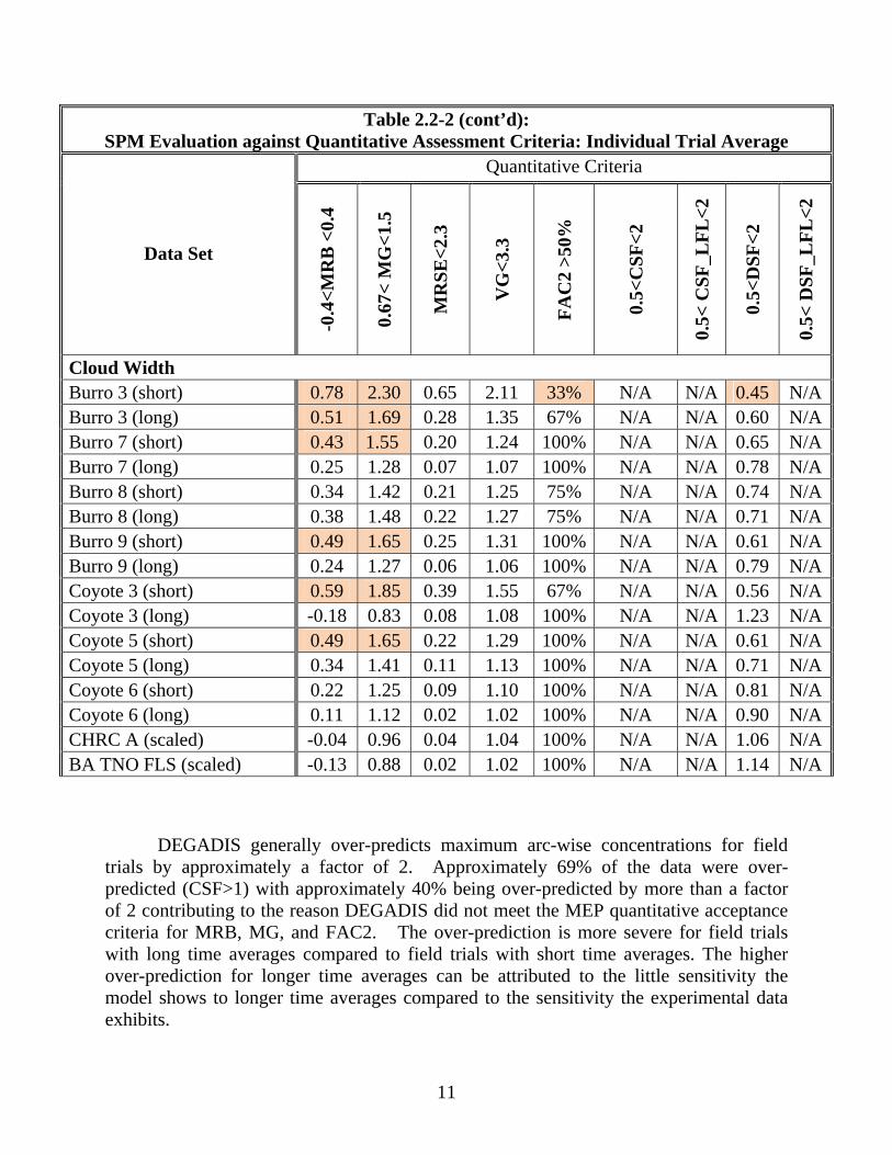
DEGADIS generally over-predicts maximum arc-wise concentrations for field trials by approximately a factor of 2. Approximately 69% of the data were over-predicted (CSF>1) with approximately 40% being over-predicted by more than a factor of 2 contributing to the reason DEGADIS did not meet the MEP quantitative acceptance criteria for MRB, MG, and FAC2. The over-prediction is more severe for field trials with long time averages compared to field trials with short time averages. The higher over-prediction for longer time averages can be attributed to the little sensitivity the model shows to longer time averages compared to the sensitivity the experimental data exhibits.

12
DEGADIS generally under-predicts concentrations for wind tunnel tests by approximately a factor of 2. All of the scaled data were under-predicted (CSF<1) with approximately 64% of the scaled data being under-predicted by more than a factor of 2 (CSF<0.5). The longer time averages associated with the wind-tunnel tests are not as likely to affect the concentrations, since the wind-tunnel tests had near steady state releases.
All the data sets met the quantitative acceptance criteria for MRSE, since generally the field trials and wind-tunnel tests showed similar trends resulting in less scatter about the mean (i.e., over-predictive of field tests and under-predictive of wind tunnel tests). Since the field trials and wind-tunnel trials had opposite trends, the VG for the trial average was higher than the MEP acceptance criteria. The larger VG attributed to field trials with long time averages is a result of some sensors being more sensitive to the longer time averages than others, resulting in some data points being over-predicted by significant margins compared to others.
DEGADIS tends to over-predict concentrations in the near field where concentrations are still high and under-predict concentrations in the far field where concentrations become low, as shown in Figure 2.2-1 and Figure 2.2-2, which compare the measured and predicted concentrations (with ideal solid line and factor of 2 dotted lines). The transition from over-predictive to under-predictive happens near the lower flammability limit (LFL) concentration (5%).

13
0.10
1.00
10.00
100.00
0.10 1.00 10.00 100.00
measured concentration (mol%)
pre
dic
ted
co
nce
ntr
ati
on
(m
ol%
)Maplin Sands 27 short
Maplin Sands 34 short
Maplin Sands 35 short
Burro 3 short
Burro 7 short
Burro 8 short
Burro 9 short
Coyote 3 short
Coyote 5 short
Coyote 6 short
ideal
+FAC2
-FAC2
Figure 2.2-1: Short Time Average Measured and Predicted Concentrations
0.10
1.00
10.00
100.00
0.10 1.00 10.00 100.00
measured concentration (mol%)
pre
dic
ted
co
nce
ntr
atio
n (
mo
l%)
Burro 3 long
Burro 7 long
Burro 8 long
Burro 9 long
TI 45 long
TI 47 long
Coyote 3 long
Coyote 5 long
Coyote 6 long
CHRC A scaled
BA Hamburg DA0120 scaled
BA Hamburg DAT223 scaled
BA Hamburg DAT647 scaled
BA Hamburg DAT631 scaled
BA Hamburg DAT632 scaled
BA Hamburg DAT637 scaled
TNO FLS scaled
ideal
+FAC2
-FAC2
Figure 2.2-2: Long Time Average Measured and Predicted Concentrations
14
DEGADIS generally meets all the MEP quantitative acceptance criteria for the maximum gas concentration arc-wise distance with the exception of the wind-tunnel tests. The reason for the better results compared to the maximum arc-wise gas concentrations is two-fold. The large over-prediction of gas concentration in the near field is mitigated by the large drop off in concentration in the near field, and the large over-prediction of gas concentration in the far field is mitigated by the smaller change in concentration in the far field. For these reasons, the distance safety factor may not be affected by seemingly large concentration discrepancies that are actually small differences in distance.
DEGADIS generally over-predicts the distance to a given concentration for field trials by approximately a factor of 1.5. Approximately 89% of the field data is predicted with a factor of 2. The over-prediction is similar for short time averages and large time averages. This can be explained by the experimental gas concentration data in the near field being affected more by longer time averaging compared to the distances to the gas concentration in the near field. DEGADIS under-predicts the distance to a given concentration for wind-tunnel tests by a factor of 1.5. Approximately 68% of the wind-tunnel data is within a factor of 2. DEGADIS predicts the maximum point-wise gas concentrations with a wide degree of scatter. DEGADIS generally seems to over-predict point-wise gas concentrations that are located closer to the cloud centerline where the maximum arc-wise concentration often occurred, and under-predict point-wise gas concentrations that are located farther from the cloud centerline. In addition, DEGADIS generally seems to under-predict short time averages and over-predict long time averages with a difference of a factor of 2 or more between them. The wide degree of scatter and inability of the DEGADIS crosswind gas concentration similarity profile to model bifurcation of clouds may make it unreliable to model point-wise gas concentrations.
DEGADIS generally meets all the MEP quantitative acceptance criteria for cloud width. DEGADIS generally over-predicts the distance to a given concentration for field trials by approximately a factor of 1.5. Approximately 84-92% of the field data is predicted with a factor of 2. DEGADIS shows better agreement with scaled wind-tunnel tests with all data within a factor of 2.
Anomalies
As shown in Figure 2.2-3, DEGADIS under-predicts the distance to the LFL for Burro 8 and Maplin Sands 34, but is well within a factor of 2.

15
0
50
100
150
200
250
300
350
400
450
500
0 100 200 300 400 500
measured distance to LFL (m)
pre
dic
ted
dis
tan
ce
to
LF
L (
m)
Maplin Sands 27 short
Maplin Sands 34 short
Maplin Sands 35 short
Burro 3 short
Burro 7 short
Burro 8 short
Burro 9 short
Coyote 3 short
Coyote 5 short
Coyote 6 short
ideal
+FAC2
-FAC2
Figure 2.2-3 Short Time Average Measured and Predicted Distance to LFL
As shown in Figure 2.2-4, Maplin Sands data comparisons indicate that the model may be less conservative for dispersion over water. The inclusion of the water transfer sub-model had negligible effect on the gas concentration, raising some question as to the validity of the water transfer sub-model. The Maplin Sands 34 is the only other LNG field trial to show under-prediction, but this is partly due to the larger amount of data points taken in the far-field, in which the model tends to be more under-predictive.
As shown in Figure 2.2-4, Burro 8 data comparisons indicate that the model may be under-predictive for low wind speed with high atmospheric stabilities, which is a larger concern due to its applicability to the 49 C.F.R. § 193.2059 requirements (2 meters per second [m/s], F stability). Comparison against longer time averages will tend to reduce the concentration of the experiment (but not the model) and make it appear conservative.

16
0.00
1.00
2.00
3.00
4.00
5.00
0.10 1.00 10.00
MG
VG
Maplin Sands 27
Maplin Sands 34
Maplin Sands 35
Burro 3
Burro 7
Burro 8
Burro 9
Coyote 3
Coyote 5
Coyote 6
FAC2 lower limit
FAC2 upper limit
Parabola
Figure 2.2-4 Short Time Average MG and VG
As shown in Figure 2.2-5, the only other low wind speed, high stability data (Thorney Island 45 and 47) indicated over-prediction. However, it was compiled using long time averages and matched closely with the Burro 8 long time average, which makes it difficult to comment as to whether under-prediction of low wind speed is a trend or not.
0.00
1.00
2.00
3.00
4.00
5.00
0.10 1.00 10.00
MG
VG
Burro 3
Burro 7
Burro 8
Burro 9
Coyote 3
Coyote 5
Coyote 6
TI 45
TI 47
CHRC A
FAC2 lower limit
FAC2 upper limit
Parabola
Figure 2.2-5 Long Time Average MG and VG

17
3.0 APPLICATION OF PHMSA ADVISORY BULLETIN ADB-10-07
This section provides a review of the DEGADIS model in accordance with the Advisory Bulletin and required supplementary documentation for obtaining approval of alternative vapor-gas dispersion models under Subpart B of 49 C.F.R. Part 193 (PHMSA, 2010) (Coldrick et al., 2010). In each of the following sections, the additional material requested by the Advisory Bulletin is reviewed and discussed.
3.1 SOURCE GEOMETRY HANDLED BY THE DISPERSION MODEL (MER SECTION 2.1.1.2; ADB-10-07 SECTION 1.A-D)
The DEGADIS model is able to simulate the dispersion of vapors emanating from ground level with zero momentum (i.e., a vaporizing liquid pool spreading axi-symmetrically). The model requires specification of a source radius and vaporization rate as a function of time. Source terms of regular geometries (e.g., circles, squares and low aspect ratio geometries) may be simplified to a circular area source term of equivalent cross-sectional area. Sources with high aspect ratios (e.g., long trenches) or irregular geometries cannot be directly inputted and may not be appropriately represented as a circular area. Therefore the model is not valid for those scenarios. Multiple source locations cannot be modeled.
DEGADIS is also able to simulate the dispersion of vapors from an elevated, vertically oriented gaseous jet source term with vertical momentum for plumes that become neutrally buoyant before reaching grade (e.g., vent stack releases and vertical pressure relief releases that do not reach grade). Horizontally oriented gaseous source terms, gaseous source terms with horizontal momentum, and gaseous source terms that may reach grade level where dense gas cloud effects may be applicable may not be accurately simulated by this model.
3.2 WIND FIELD (MER SECTION 2.2.2.1; ADB-10-07 SECTION 2)
The DEGADIS model is able to simulate steady state wind profiles. The model is not able to simulate transient wind speed or direction. Low wind speeds (less than 2 m/s) can be modeled, but may not be handled well by the model and may result in under-prediction of the hazard distance.
3.3 STRATIFICATION (MER SECTION 2.2.2.3; ADB-10-07 SECTION 3)
In the DEGADIS model, the Monin-Obukhov length is calculated automatically based on the Pasquill-Gifford category specified (A, B, C, D, E, or F). Specifying a different Monin-Obukhov length is also possible and will supersede any calculated value. Temperature and/or turbulence profiles cannot be inputted by the user. High atmospheric stability (F stability) can be modeled, but may not be handled well by the model and may result in under-prediction of the hazard distance.

18
3.4 TERRAIN TYPES AVAILABLE (MER SECTION 2.2.3.1; ADB-10-07 SECTION 4) & COMPLEX EFFECTS (MER SECTION 2.3.1.2; ADB-10-07 SECTION 4)
The DEGADIS model is limited to dispersion over unobstructed level terrain with uniform roughness length specified by the user. Sloped or varying terrain will affect the gravity spreading of a dense gas release. For dense gas releases, such as LNG vapor, the cloud will be stretched out as the dense gas plume flows along downward slopes. Therefore, for downward slopes, the centerline concentrations may be over-predicted in the near field, but under-predicted in the far field. Correspondingly, cross-wise concentrations and cloud widths may be over-predicted in the near field, but under-predicted in the far field. In contrast, upward slopes will oppose the movement of the dense gas, causing the vapor to accumulate and spread perpendicular to the upward slope. Therefore, for upward slopes, the centerline concentrations may be under-predicted in the near field, but over-predicted in the far field. Correspondingly, cross-wise concentrations and cloud widths may be under-predicted in the near field, but over-predicted in the far field. DEGADIS was not validated against sloped terrain tests, since it is not designed to simulate those scenarios.
3.5 OBSTACLE TYPES AVAILABLE (MER SECTION 2.2.4.1; ADB-10-07 SECTION 5) & COMPLEX EFFECTS (MER SECTION 2.4.3.1; ADB-10-07 SECTION 5)
The model is limited to dispersion over unobstructed level terrain with uniform roughness length specified by the user. For most instances, downwind concentrations assuming unobstructed terrain will be over-predictive. However, there are instances where downwind concentrations could be under-predictive due to wind channeling effects (Melton & Cornwell, 2009). Wind channeling may occur between adjacent LNG storage tanks, buildings, or large structures, which may result in the model being under-predictive for LNG vapor concentrations.
3.6 TURBULENCE MODELING (MER SECTION 2.3.1.5; ADB-10-07 SECTION 6)
The DEGADIS model parameterizes turbulence based on empirical turbulence coefficients formed from the user-specified atmospheric parameters (horizontal turbulent diffusivity) and Richardson number (vertical turbulent diffusivity).
The parameterization for horizontal turbulence is based on functions of the Pasquill stability category and averaging time. As averaging time increases, different empirical coefficients are used.
For Richardson numbers greater than zero, the parameterization for vertical turbulence is based on laboratory scale data for vertical mixing in stable density stratified

19
fluid flows reported by Kantha et al (1977), Lofquist (1960), and McQuaid (1976) (Havens, Spicer 1990). For Richardson numbers less than zero, the function is taken from Colenbrander and Puttock (1983) and modified so the passive limits of the two functions agree (Havens, Spicer, 1990). When heat transfer from the surface is present, vertical mixing is enhanced by convection turbulence and is parameterized based on work by Zeman and Tennekes (1977) (Havens, Spicer, 1990).
The plume model has separate parameterizations for turbulence caused by jet effects. For area source terms, the parameterization of turbulence is a simplification based on unobstructed stably stratified flows. Therefore, it would not be appropriate for use in situations where obstructions are to be considered or where source terms with high momentum (i.e., jet releases) that may result in additional turbulence exist. For jet source terms, the parameterization of turbulence is based on jet effects and does not account for turbulence associated with impingement of a jet or with a dense vapor cloud reaching grade, and therefore would not be appropriate for releases that impinge on surfaces or reach grade.
3.7 BOUNDARY CONDITIONS (MER SECTION 2.3.1.7; ADB-10-07 SECTION 7)
The model requires the user to specify: the source term as a radius and vaporization rate at different time intervals; the wind profile in terms of the Pasquill-Gifford category (or Monin-Obukhov length); and the surface roughness. Zero velocity is imposed at the ground boundary condition. No other boundary conditions are able to be specified by the user.
3.8 COMPLEX EFFECTS: AEROSOLS (MER SECTION 2.3.1.1; ADB-10-07 SECTION 8)
Using DEGADIS, flashed vapors may be treated as gaseous jet source terms. However, for jet source terms, DEGADIS assumes a vertically oriented release with vertical momentum. DEGADIS also does not account for turbulence generated from plumes that reach grade or releases that impinge onto surfaces. Therefore, jet source terms, horizontally oriented gaseous source terms, gaseous source terms with horizontal momentum, and gaseous source terms that may reach grade level may not be accurately simulated by this model.
The model is not able to explicitly simulate the formation, vaporization, rainout, or subsequent dispersion of aerosol droplets. Hanna, et al. (1993) has attempted to simulate the dispersion of evaporated aerosol by specifying a source term based on the density of the vapor-aerosol-air mixture and the mole fraction of vapor-aerosol in the cloud (based on the corresponding mass concentration of the vapor-aerosol) obtained by assuming complete adiabatic mixing.

20
3.9 COMPUTATIONAL MESH (MER SECTION 2.4.3.1; ADB-10-07 SECTION 9)
As use of a computational mesh is not related to integral models such as DEGADIS, this section is not applicable.
3.10 DISCRETIZATION METHODS (MER SECTION 2.4.2.3; ADB-10-07 SECTION 10)
DEGADIS solves ordinary differential equations using the Runge-Kutta method with a variable step that is 4th order accurate. This is one of the oldest and probably the most commonly used numerical method for integral type models. More accurate numerical solution methodologies now exist, but are not expected to have a great effect on the results.
3.11 SOURCES OF MODEL UNCERTAINTY (MER SECTION 2.6; ADB-10-07, SECTION 11)
All models contain simplifications to minimize the computational time, which causes a certain degree of uncertainty and limits the applicability of the model. The areas of uncertainty for the DEGADIS model would be the numerical solver used to discretize the space, the source term simplification, the steady state wind profile simplification, and the turbulence parameterization.
3.12 SENSITIVITY TO INPUT (MER SECTION 2.6.4; ADB-10-07 SECTION 12)
A sensitivity analysis of the DEGADIS model was conducted based on the various inputs that could be specified, including source term, wind speed, surface roughness, atmospheric stability (and/or Monin-Obukhov Length), ambient temperature, ambient pressure, ambient relative humidity, and molecular weight. The sensitivity of the model was determined based on respective uncertainties for those values. Each sensitivity case is denoted by a corresponding letter and number. The letter corresponds to a different source term and the number designates the inputted variables as shown in Table 3.12-1.
The base case assumes values provided in the MEP, which were verified with the
original data series reports available (Goldwire et al 1983a), (Goldwire, et al 1983b), (Koopman et al 1982a), (Koopman et al 1982b), (Colenbrander et al 1984a), (Colenbrander et al 1984b), (Colenbrander et al 1984c), (Johnson, 1985). Notes have been provided in the validation database for instances where there were conflicts between the MEP and original data series reports. The original data series reports were utilized to generate the sensitivity bounds for the inputs into DEGADIS. The lower and upper sensitivity bounds were based upon the lower and upper quartiles of the data. Where the lower and upper quartiles did not vary by more than 10% from the mean, no sensitivity analysis was conducted (e.g., a_10 and a_13). Since the wind tunnel tests were
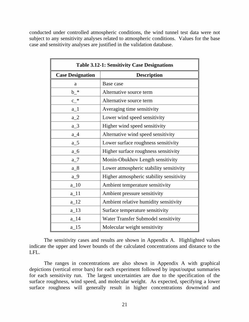
21
conducted under controlled atmospheric conditions, the wind tunnel test data were not subject to any sensitivity analyses related to atmospheric conditions. Values for the base case and sensitivity analyses are justified in the validation database.
Table 3.12-1: Sensitivity Case Designations
Case Designation Description
a Base case
b_* Alternative source term
c_* Alternative source term
a_1 Averaging time sensitivity
a_2 Lower wind speed sensitivity
a_3 Higher wind speed sensitivity
a_4 Alternative wind speed sensitivity
a_5 Lower surface roughness sensitivity
a_6 Higher surface roughness sensitivity
a_7 Monin-Obukhov Length sensitivity
a_8 Lower atmospheric stability sensitivity
a_9 Higher atmospheric stability sensitivity
a_10 Ambient temperature sensitivity
a_11 Ambient pressure sensitivity
a_12 Ambient relative humidity sensitivity
a_13 Surface temperature sensitivity
a_14 Water Transfer Submodel sensitivity
a_15 Molecular weight sensitivity
The sensitivity cases and results are shown in Appendix A. Highlighted values indicate the upper and lower bounds of the calculated concentrations and distance to the LFL.
The ranges in concentrations are also shown in Appendix A with graphical depictions (vertical error bars) for each experiment followed by input/output summaries for each sensitivity run. The largest uncertainties are due to the specification of the surface roughness, wind speed, and molecular weight. As expected, specifying a lower surface roughness will generally result in higher concentrations downwind and

22
subsequently longer distances to the LFL and vice versa. As expected, specifying a lower wind speed will generally result in higher concentrations downwind and subsequently longer distances to the LFL and vice versa. Specifying a lighter molecular weight of LNG (i.e., as methane) generally will result in higher concentrations downwind and subsequently longer distances to the LFL and vice versa. Overall, the concentrations may differ by more than a factor of four and downwind dispersion distances to the LFL may differ by up to a factor of two, dependant on the uncertainty in the user input and sensitivity to that input.
3.13 LIMITS OF APPLICABILITY (MER SECTION 2.7; ADB-10-07 SECTION 13)
The DEGADIS model is limited to dispersion over unobstructed level terrain with uniform roughness length specified by the user. The model cannot accurately simulate obstructed, sloped or varying terrain or terrain with varying surface roughness length.
The model does not have a built-in source term model and requires user-input to describe the source term. The source terms that can be defined are: (1) a single regularly shaped area source term with no momentum with specified equivalent radius and vaporization rate with respect to time (i.e., a single steady state or spreading vaporizing pool); or (2) an elevated vertically oriented gaseous jet source term with vertical momentum for plumes that become neutrally buoyant before reaching grade with specified diameter, elevation, release rate, and duration of release (i.e., a single time-limited elevated gaseous jet from a vent stack, pressure relief valve). Flashed vapors may be treated as gaseous source terms, where appropriate. Aerosol formation, vaporization, rainout, or subsequent dispersion of aerosol droplets cannot be modeled explicitly by the model, but alternative approaches may be suitable subject to further evaluation. The model cannot model multiple source terms that may occur simultaneously, nor can it accurately simulate a single source term with a highly irregular geometry or high aspect ratio (e.g., trenches). The model is not able to simulate horizontally oriented gaseous source terms, gaseous source terms with horizontal momentum, or gaseous source terms that may reach grade level where dense gas cloud effects may be applicable.

23
3.14 EVALUATION AGAINST THE MEP QUANTITATIVE ASSESSMENT CRITERIA (MER SECTION 6.2.4; ADB-10-07 SECTION 14)
3.14.1 Uncertainty Analysis of Model Input
This series of uncertainty analyses accounts for model uncertainty due to uncertainty in the assumption of input parameters specified by the user. This subtopic is further broken down into seven areas.
i. Analysis of source term(s)
The DEGADIS model does not have a built-in source term model and requires the specification of the source diameter and vaporization rate as a function of time.
For experiments involving LNG spills over water, this model validation study used
the ABS (American Bureau of Shipping)/FERC LNG pool spread source term model to determine pool diameter and vaporization rates as a function of time (FERC, 2004a) (FERC, 2004b). The ABS/FERC LNG pool spread model assumes a 0.167 kg/m2/sec vaporization rate based on empirical data for spills over water. For all other experiments the specified pool diameters and rates were used and no sensitivity analysis was performed.
For the Thorney Island and wind tunnel trials, the gas was released through a well
defined opening at ground level that was designed to give a release with negligible vertical momentum. The source term was defined based on this information without any need for additional sensitivity analyses. This approach is similar to previous validation studies (Hanna, et al 1993).
For experiments involving LNG spills over water, a sensitivity analysis was
conducted to examine the effect of pool spread velocity. The ABS/FERC model, which models the pool spread and specifies a vaporization of 0.167kg/m2/sec was compared to an instantaneously formed steady-state pool (i.e. spreads instantaneously) using the same vaporization rate.
A sensitivity analysis was also conducted to examine the effect of the vaporization
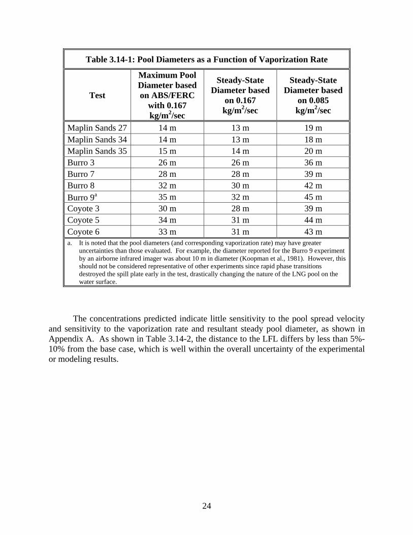
rate. A source term based on an instantaneously formed steady-state pool using a vaporization rate of 0.167 kg/m2/sec was compared to an instantaneously formed steady-state pool using a vaporization rate of 0.085 kg/m2/sec. The 0.085 kg/m2/sec vaporization rate has been commonly used in previous validation studies, and is based on visual observations of the steady-state pool size and spill rate during the Maplin Sands experiments (Puttock, 1987). The resultant pool diameters are shown in Table 3.14-1.
24
Table 3.14-1: Pool Diameters as a Function of Vaporization Rate
Test
Maximum Pool Diameter based on ABS/FERC
with 0.167 kg/m2/sec
Steady-State Diameter based
on 0.167 kg/m2/sec
Steady-State Diameter based
on 0.085 kg/m2/sec
Maplin Sands 27 14 m 13 m 19 m Maplin Sands 34 14 m 13 m 18 m Maplin Sands 35 15 m 14 m 20 m Burro 3 26 m 26 m 36 m Burro 7 28 m 28 m 39 m Burro 8 32 m 30 m 42 m Burro 9a 35 m 32 m 45 m Coyote 3 30 m 28 m 39 m Coyote 5 34 m 31 m 44 m Coyote 6 33 m 31 m 43 m a. It is noted that the pool diameters (and corresponding vaporization rate) may have greater
uncertainties than those evaluated. For example, the diameter reported for the Burro 9 experiment by an airborne infrared imager was about 10 m in diameter (Koopman et al., 1981). However, this should not be considered representative of other experiments since rapid phase transitions destroyed the spill plate early in the test, drastically changing the nature of the LNG pool on the water surface.
The concentrations predicted indicate little sensitivity to the pool spread velocity and sensitivity to the vaporization rate and resultant steady pool diameter, as shown in Appendix A. As shown in Table 3.14-2, the distance to the LFL differs by less than 5%-10% from the base case, which is well within the overall uncertainty of the experimental or modeling results.

25
Table 3.14-2:
Distance to LFL Uncertainty Due to Pool Spread Velocity and Vaporization Rate
Test Arc
ABS/FERC Pool Spread Model
with 0.167 kg/m2/sec
Steady-State Diameter based
on 0.167 kg/m2/sec
Steady-State Diameter based
on 0.085 kg/m2/sec
Maplin Sands 27
204 m to LFL 206 m to LFL 216 m to LFL
Maplin Sands 34
191 m to LFL 191 m to LFL 191 m to LFL
Maplin Sands 35
223 m to LFL 222 m to LFL 202 m to LFL
Burro 3 405 m to LFL 402 m to LFL 394 m to LFL
Burro 7 388 m to LFL 387 m to LFL 368 m to LFL
Burro 8 289 m to LFL 291 m to LFL 308 m to LFL
Burro 9 492 m to LFL 482 m to LFL 465 m to LFL
Coyote 3 392 m to LFL 392 m to LFL 385 m to LFL
Coyote 5 396 to LFL 387 to LFL 358 to LFL
Coyote 6 457 m to LFL 455 m to LFL 451 m to LFL

26
ii. Analysis of boundary conditions
The DEGADIS model requires the user to specify the following items: the inlet boundary as a source term radius and vaporization rate at different time intervals (i.e. source term); the wind profile based on the Pasquill-Gifford (or Monin-Obukhov length) ; and the surface roughness. Zero velocity is imposed at the ground boundary condition. No other boundary conditions are specified by the user. The source term and wind profile boundary sensitivities are discussed in sections i and iii, respectively.
iii. Analysis of wind profile.
The DEGADIS model is only able to simulate steady state wind profiles and direction. For all trials, the wind speed used for the base case was defined as the domain average wind speeds from the MEP, which were verified to match the domain average wind sensor data during the dispersion periods found in the original data series reports, where available (Goldwire et al 1983a), (Goldwire, et al 1983b), (Koopman et al 1982a), (Koopman et al 1982b), (Colenbrander et al 1984a), (Colenbrander et al 1984b), (Colenbrander et al 1984c), (Johnson, 1985). Similarly, the upper and lower bounds for the wind speed were based on the upper and lower quartiles of the domain average wind sensor data during the dispersion periods found in the original data series reports, where available (Goldwire et al 1983a), (Goldwire, et al 1983b), (Koopman et al 1982a), (Koopman et al 1982b), (Colenbrander et al 1984a), (Colenbrander et al 1984b), (Colenbrander et al 1984c), (Johnson, 1985). Given the little fluctuation and/or uncertainty (<10% of mean) in some of the data, certain sensitivity cases were not simulated. In Maplin Sands 27, the original data series report (Colenbrander et al 1984a) claims that the wind speed sensor at 250 m, -90 deg, 10 m,, which recorded a 6.1 m/s mean (270-430 sec), probably represents the environmental conditions best, since the plume was blown in the direction of this pontoon. Accordingly, a number of reports list 6.1 m/s as the mean wind speed, while other reports list 5.5-5.6 m/s as the mean (190-350 sec) wind speed. Coincidentally, the upper quartile of the domain average wind sensor data provided in the original data series reports is 6.2 m/s. For consistency, the base case was taken as the 5.6 m/s domain averaged sensor data provided in the original data series reports and listed in the MEP. In addition, where the domain average wind sensor data reported in the MEP differed from the wind speed provided in the MEP, an additional case was simulated (a_4).
The upper and lower bounds for the stability class were based upon the atmospheric conditions (e.g. wind speed, cloud cover, insolation, time of day, etc). Wind speed data and atmospheric conditions were used in conjunction with various guidance documents, including the DEGADIS 2.1 documentation (Havens, Spicer, 1990), to determine the wind stability.

27
The surface roughness values for the base case were taken from the MEP (Coldrick et al., 2010) (Ivings et al., 2007). For field trials, surface roughness is rarely known to better than an order of magnitude (Johnson, 1985)). Where uncertainty or disagreement of the surface roughness existed, a sensitivity analysis to surface roughness was carried out. This effort was based on the bounds generated from the DEGADIS 2.1 documentation (Havens et al 1990) and recommended and generally accepted good engineering practices, which in certain circumstances varied greatly from that specified in the MEP (Coldrick et al., 2010). Previous validation studies conducted for the experiments were also examined (Hanna et al., 1993) (Ermak et al., 1989) (Puttock et al., 1984).
Maplin Sands
The MEP reports a surface roughness of 0.0003 meter (m) for Maplin Sands, which was conducted over waters protected by a bund (during periods of low tide) (Coldricket al., 2010). The Modeler’s Data Archive (MDA) reports a value of 0.0003 m (Hanna et al., 1993). Ermak et al. (1989) reports a surface roughness of 0.000058 m. The Maplin Sands Reports provides a surface roughness estimate of 0.00002 m based on a 1:20 scale wind tunnel experiment to determine the effect on the surface roughness from the pontoons that were fitted with the sensor arrays (Puttock et al., 1984) (Colenbrander et al., 1984a), (Colenbrander et al., 1984b), (Colenbrander et al., 1984c). Based on photographic observations of the test site, most users could reasonably assume the surface roughness to correspond to open calm water or sea in coastal areas. The DEGADIS reports surface roughness of 0.0001 m for calm open seas and 0.001 m for sea in coastal areas (Spicer, Havens, 1982), (Havens, Spicer, 1990). Brutsaert reports 0.0001 m to 0.0006 m for large water surfaces (Brutstaert, 1982). The base case used the value of 0.0003 m reported in the MEP; a sensitivity analysis was conducted using 0.0001 m and 0.001 m. A third simulation was ran specifying the Monin-Obukhov lengths provided in the MEP. It should also be noted that all the Maplin Sands tests were conducted at low tide, where the 300 m low-lying bund may have affected the surface roughness and dispersion. The pontoons equipped with the sensor arrays would also have an influence on the dispersion.
Given the uncertainty in the surface roughness length that could be reasonably chosen, there was a moderate difference in downwind concentrations, as shown in Appendix A. As shown in Table 3.14-3, the distance to the LFL differs approximately 5-15% from the base case, which is within the overall uncertainty of the experimental or modeling results. As expected, specifying a higher surface roughness generally results in lower concentrations and shorter distances to the LFL.

28
Table 3.14-3:
Distance to LFL Uncertainty Due To Surface Roughness Length: Maplin Sands
Test Base Case 0.0003 m
Lower Bound 0.0001 m
Upper Bound 0.001 m
Maplin Sands 27 204 m to LFL 214 m to LFL 175 m to LFL Maplin Sands 34 191 m to LFL 184 m to LFL 176 m to LFL Maplin Sands 35 223 m to LFL 246 m to LFL 200 m to LFL
Burro and Coyote
The MEP reports a surface roughness of 0.0002 m for Burro and Coyote, which were conducted over a spill pond surrounded by desert terrain. The spill pond was 58 m in diameter and 1.5 m below the surrounding terrain. The surrounding terrain had a slight upward slope rising 7 m above the water level at a downwind distance of about 80 m before leveling out thereafter (Coldrick et al., 2010). The MDA reports a value of 0.0002 m (Hanna et al., 1993). Ermak et al (1989) also reports a surface roughness of 0.0002 m. The Burro and Coyote Series Reports reports a value of 0.000205 m (Koopman et al., 1982a) (Koopman et al., 1982b) (Goldwire et al., 1983a) (Goldwire et al., 1983b) Based on photographic observations of the test site, users could reasonably assume the surface roughness to correspond to a desert or an area with sparse vegetation (Koopman et al., 1982c). The DEGADIS documentation reports surface roughness of 0.0005 m for desert and 0.01 m for few trees, winter time (Spicer, Havens 1990). Pielke (2002) reports 0.0003m for smooth deserts and 0.01m surface roughness value for the upper range of soils and short grass. Brutsaert (1982) reports 0.04 m for grass with some bushes and trees. The base case used the value of 0.0002 m reported in the MEP (Coldrick et al., 2010); a sensitivity analysis was conducted using 0.01 m. Simulations were also run specifying the Monin-Obukhov lengths provided in the MEP.
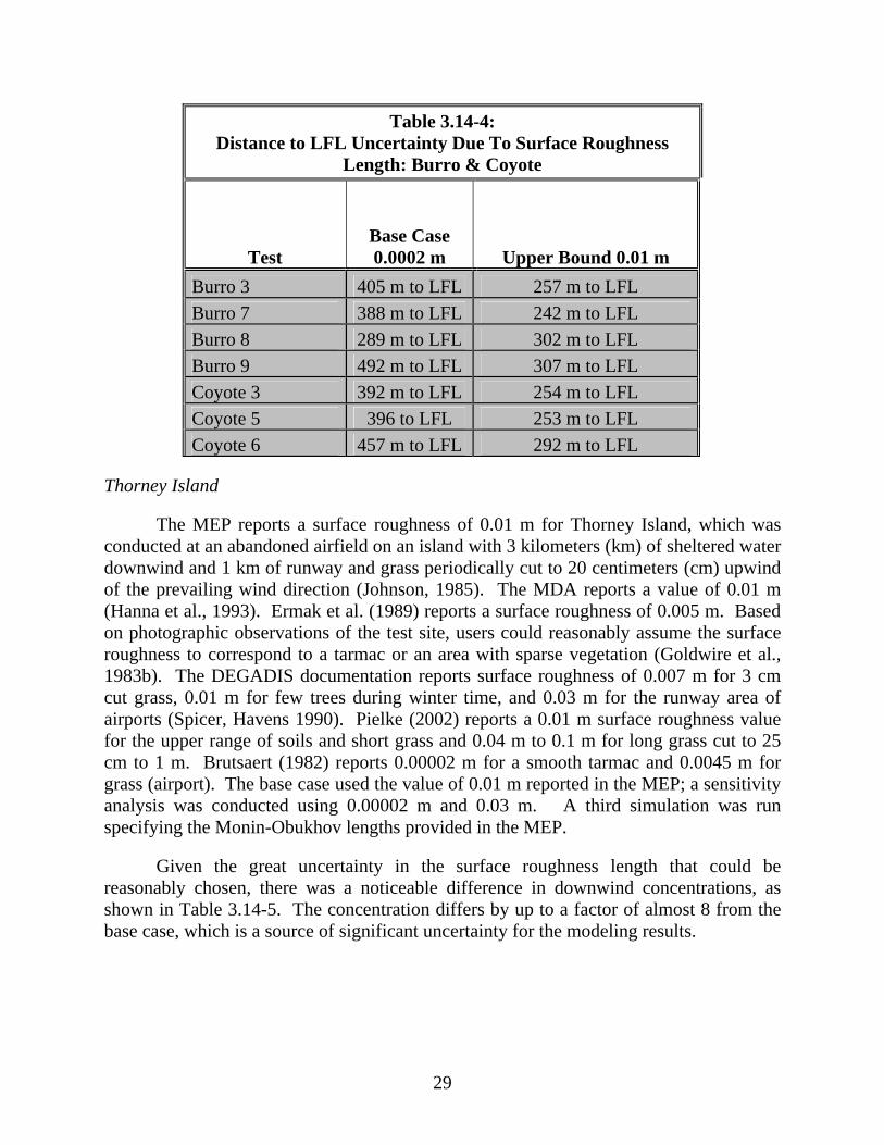
Given the great uncertainty in the surface roughness length that could be reasonably chosen, there was a noticeable difference in downwind concentrations, as shown in Appendix A. As shown in Table 3.14-4, the distance to the LFL differs by up to 40% from the base case, which is a source of significant uncertainty for the modeling results. With the exception of Burro 8, which was the only low-wind speed F stability test, the larger surface roughness resulted in lesser concentrations and a shorter distance to the LFL.
29
Table 3.14-4: Distance to LFL Uncertainty Due To Surface Roughness
Length: Burro & Coyote
Test Base Case 0.0002 m Upper Bound 0.01 m
Burro 3 405 m to LFL 257 m to LFL
Burro 7 388 m to LFL 242 m to LFL
Burro 8 289 m to LFL 302 m to LFL
Burro 9 492 m to LFL 307 m to LFL
Coyote 3 392 m to LFL 254 m to LFL
Coyote 5 396 to LFL 253 m to LFL
Coyote 6 457 m to LFL 292 m to LFL
Thorney Island
The MEP reports a surface roughness of 0.01 m for Thorney Island, which was conducted at an abandoned airfield on an island with 3 kilometers (km) of sheltered water downwind and 1 km of runway and grass periodically cut to 20 centimeters (cm) upwind of the prevailing wind direction (Johnson, 1985). The MDA reports a value of 0.01 m (Hanna et al., 1993). Ermak et al. (1989) reports a surface roughness of 0.005 m. Based on photographic observations of the test site, users could reasonably assume the surface roughness to correspond to a tarmac or an area with sparse vegetation (Goldwire et al., 1983b). The DEGADIS documentation reports surface roughness of 0.007 m for 3 cm cut grass, 0.01 m for few trees during winter time, and 0.03 m for the runway area of airports (Spicer, Havens 1990). Pielke (2002) reports a 0.01 m surface roughness value for the upper range of soils and short grass and 0.04 m to 0.1 m for long grass cut to 25 cm to 1 m. Brutsaert (1982) reports 0.00002 m for a smooth tarmac and 0.0045 m for grass (airport). The base case used the value of 0.01 m reported in the MEP; a sensitivity analysis was conducted using 0.00002 m and 0.03 m. A third simulation was run specifying the Monin-Obukhov lengths provided in the MEP.
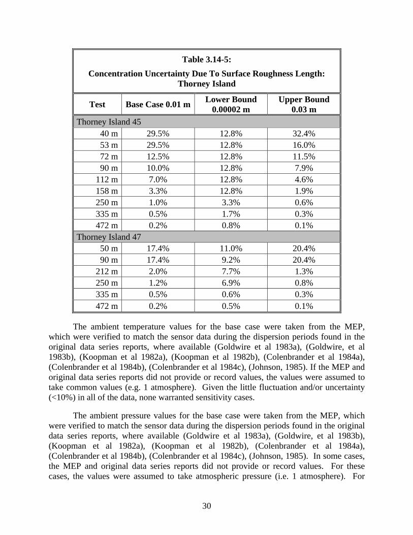
Given the great uncertainty in the surface roughness length that could be reasonably chosen, there was a noticeable difference in downwind concentrations, as shown in Table 3.14-5. The concentration differs by up to a factor of almost 8 from the base case, which is a source of significant uncertainty for the modeling results.
30
Table 3.14-5:
Concentration Uncertainty Due To Surface Roughness Length: Thorney Island
Test Base Case 0.01 mLower Bound
0.00002 m Upper Bound
0.03 m
Thorney Island 45 40 m 29.5% 12.8% 32.4% 53 m 29.5% 12.8% 16.0% 72 m 12.5% 12.8% 11.5% 90 m 10.0% 12.8% 7.9%
112 m 7.0% 12.8% 4.6% 158 m 3.3% 12.8% 1.9% 250 m 1.0% 3.3% 0.6% 335 m 0.5% 1.7% 0.3% 472 m 0.2% 0.8% 0.1%
Thorney Island 47 50 m 17.4% 11.0% 20.4% 90 m 17.4% 9.2% 20.4%
212 m 2.0% 7.7% 1.3% 250 m 1.2% 6.9% 0.8% 335 m 0.5% 0.6% 0.3% 472 m 0.2% 0.5% 0.1%
The ambient temperature values for the base case were taken from the MEP, which were verified to match the sensor data during the dispersion periods found in the original data series reports, where available (Goldwire et al 1983a), (Goldwire, et al 1983b), (Koopman et al 1982a), (Koopman et al 1982b), (Colenbrander et al 1984a), (Colenbrander et al 1984b), (Colenbrander et al 1984c), (Johnson, 1985). If the MEP and original data series reports did not provide or record values, the values were assumed to take common values (e.g. 1 atmosphere). Given the little fluctuation and/or uncertainty (<10%) in all of the data, none warranted sensitivity cases.
The ambient pressure values for the base case were taken from the MEP, which were verified to match the sensor data during the dispersion periods found in the original data series reports, where available (Goldwire et al 1983a), (Goldwire, et al 1983b), (Koopman et al 1982a), (Koopman et al 1982b), (Colenbrander et al 1984a), (Colenbrander et al 1984b), (Colenbrander et al 1984c), (Johnson, 1985). In some cases, the MEP and original data series reports did not provide or record values. For these cases, the values were assumed to take atmospheric pressure (i.e. 1 atmosphere). For
31
cases that did provide or record ambient pressure, the fluctuation was insignificant (<10%), and most cases would not warrant sensitivity cases. However, typically site specific values for ambient pressure are not available and atmospheric (i.e. 1 atmosphere) is assumed. To gauge this common assumption and determine the sensitivity of the model to this parameter, sensitivity cases were run where the ambient pressure differed from 1 atmosphere.
The ambient relative humidity values for the base case were taken from the MEP, which were verified to match the sensor data during the dispersion periods found in the original data series reports, where available (Goldwire et al 1983a), (Goldwire, et al 1983b), (Koopman et al 1982a), (Koopman et al 1982b), (Colenbrander et al 1984a), (Colenbrander et al 1984b), (Colenbrander et al 1984c), (Johnson, 1985). In some cases, the ambient relative humidity data listed in the MEP differed from the relative humidity sensor data provided in the original data series reports. In Maplin Sands 34, it is noted that the original data series report (Colenbrander et al 1984a) provides values of 72% at Maplin Sands test site and 74% at Foulness Met. Station (corrected to Maplin Sands site temp), which was located 5 km away in SW direction and about 1 km inland. The relative humidity sensor data showed a range from 70 to 77%. It is unclear where the 90% value listed in the MEP originated. For that reason, the base case was taken as the 72% average value provided in the original data series, and a sensitivity case to 90% relative humidity was provided. There was little fluctuation and/or uncertainty (<10%) in most of data, hence most cases did not warrant sensitivity cases, denoted N/A. However, typically site specific values for weather data are not available and nearby weather stations are relied upon. For this reason, sensitivity cases were also run where nearby weather station data was provided in the original data series report, such as the Maplin Sands trials.
The surface/ground temperature values for the base case were taken from the MEP, which were verified to match the sensor data during the dispersion periods found in the original data series reports, where available (Goldwire et al 1983a), (Goldwire, et al 1983b), (Koopman et al 1982a), (Koopman et al 1982b), (Colenbrander et al 1984a), (Colenbrander et al 1984b), (Colenbrander et al 1984c), (Johnson, 1985). If the MEP and original data series reports did not provide or record values, the values were assumed to take the temperature of the ambient temperature. Given the little fluctuation and/or uncertainty (<10%) in all of the data, none warranted sensitivity cases. In addition, the water transfer submodel within DEGADIS was used in the Maplin Sands trials. A sensitivity to the inclusion of this submodel was included for Maplin Sands.
The molecular weight values for the base case were taken from the MEP, which were verified to match the sensor data during the dispersion periods found in the original data series reports, where available (Goldwire et al 1983a), (Goldwire, et al 1983b), (Koopman et al 1982a), (Koopman et al 1982b), (Colenbrander et al 1984a), (Colenbrander et al 1984b), (Colenbrander et al 1984c), (Johnson, 1985). For the LNG

32
field trials, the lower bound for the molecular weight was based on the molecular weight of methane assuming preferential boiloff; no upper bound was provided, as heavier molecular weights would not be expected than those listed in the MEP. Given the little fluctuation and/or uncertainty (<10%) in some of these values, some cases did not warrant sensitivity cases, denoted N/A.
The inputs for each sensitivity case utilized are summarized in Table 3.14-6. The inputs and outputs for each trial are shown in Appendix A.

33
Table 3.14-6: Sensitivity Case Inputs
Maplin Sands 27
Maplin Sands 34
Maplin Sands 35
Burro 3 Burro 7 Burro 8 Burro 9 Coyote 3 Coyote 5 Coyote 6 Thorney Island 45
Thorney Island 47
Source Term Base Case 0.167kg/m^2/sec
ABS/FERC 0.167kg/m^2/sec ABS/FERC
0.167kg/m^2/sec ABS/FERC
0.167kg/m^2/sec ABS/FERC
0.167kg/m^2/sec ABS/FERC
0.167kg/m^2/sec ABS/FERC
0.167kg/m^2/sec ABS/FERC
0.167kg/m^2/sec ABS/FERC
0.167kg/m^2/sec ABS/FERC
0.167kg/m^2/sec ABS/FERC
MEP MEP
Alternative 1 0.167kg/m^2/sec steady state
0.167kg/m^2/sec steady state
0.167kg/m^2/sec steady state
0.167kg/m^2/sec steady state
0.167kg/m^2/sec steady state
0.167kg/m^2/sec steady state
0.167kg/m^2/sec steady state
0.167kg/m^2/sec steady state
0.167kg/m^2/sec steady state
0.167kg/m^2/sec steady state
N/A N/A
Alternative 2 0.085kg/m^2/sec steady state
0.085kg/m^2/sec steady state
0.085kg/m^2/sec steady state
0.085kg/m^2/sec steady state
0.085kg/m^2/sec steady state
0.085kg/m^2/sec steady state
0.085kg/m^2/sec steady state
0.085kg/m^2/sec steady state
0.085kg/m^2/sec steady state
0.085kg/m^2/sec steady state
N/A N/A
Wind Speed Base Case 5.6 (MEP) 8.5 (MEP) 9.6 (MEP) 5.4 (MEP) 8.4 (MEP) 1.8 (MEP) 5.7 (MEP) 6 (MEP) 9.7 (MEP) 4.6 (MEP) 2.3 (MEP) 1.5 (MEP) Lower Bound 4.4 (25% quart.) 7.6 (25% quart.) 7.9 (25% quart.) 5.1 (25% quart.) N/A 1.5 (25% quart.) N/A N/A N/A N/A N/A N/A Upper Bound 6.1 (75% quart.) 9.5 (75% quart.) 11 (75% quart.) 5.8 (75% quart.) N/A 2 (75% quart.) N/A N/A N/A N/A N/A N/A Atmospheric Stability
Base Case C-D (MEP) D (MEP) D (MEP) C (MEP) D (MEP) E (MEP) D (MEP) C (MEP) C (MEP) D (MEP) E-F (MEP) F (MEP) Lower Bound D (assumed) N/A N/A N/A N/A F (assumed) N/A N/A D (assumed) E (assumed) F (assumed) N/A Upper Bound C (assumed) C (assumed) C (assumed) N/A C (assumed) N/A C (assumed) N/A N/A N/A E (assumed) E (assumed) Surface/Ground Roughness
Base Case 3e-4 (MEP) 3e-4 (MEP) 3e-4 (MEP) 2e-4 (MEP) 2e-4 (MEP) 2e-4 (MEP) 2e-4 (MEP) 2e-4 (MEP) 2e-4 (MEP) 2e-4 (MEP) 1e-2 (MEP) 1e-2 (MEP) Lower Bound 1e-4 (assumed) 1e-4 (assumed) 1e-4 (assumed) N/A N/A N/A N/A N/A N/A N/A 2e-5
(assumed) 2e-5 (assumed)
Upper Bound 1e-3 (assumed) 1e-3 (assumed) 1e-3 (assumed) 1e-2 (assumed) 1e-2 (assumed) 1e-2 (assumed) 1e-2 (assumed) 1e-2 (assumed) 1e-2 (assumed) 1e-2 (assumed) 3e-2 (assumed)
3e-2 (assumed)
Ambient Temperature
Base Case 288.1K (MEP) 288.4K (MEP) 289.3K (MEP) 307.75K (MEP) 306.96 (MEP) 306.02 (MEP) 308.52K (MEP) 311.45K (MEP) 301.49K (MEP) 297.26K (MEP) 286.25K (MEP)
287.45K (MEP)
Lower Bound N/A N/A N/A N/A N/A N/A N/A N/A N/A N/A N/A N/A Upper Bound N/A N/A N/A N/A N/A N/A N/A N/A N/A N/A N/A N/A Ambient Pressure
Base Case 1 (assumed) 1 (assumed) 1 (assumed) 0.936 (MEP) 0.928 (MEP) 0.929 (MEP) 0.928 (MEP) 0.924 (MEP) 0.927 (MEP) 0.930 (MEP) 1 (MEP) 1 (MEP) Lower Bound N/A N/A N/A N/A N/A N/A N/A N/A N/A N/A N/A N/A Upper Bound N/A N/A N/A N/A 1 (assumed) 1 (assumed) 1 (assumed) 1 (assumed) 1 (assumed) 1 (assumed) N/A Ambient Relative Humidity
Base Case 53 (MEP) 72 (avg. data) 63 (avg. data) 5.2 (MEP) 7.4 (MEP) 4.5 (MEP) 14.4 (MEP) 11.3 (MEP) 22.1 (MEP) 22.8 (MEP) 100 (MEP) 97.4 (MEP) Lower Bound N/A N/A N/A N/A 5 N/A 6.5 3.5 7.2 4.5 N/A N/A Upper Bound 63 (avg.
Foulness) 90 (MEP) 77 (MEP) N/A N/A N/A N/A N/A N/A N/A N/A N/A
Molecular Weight
Base Case 17.23 (MEP) 16.66 (MEP) 16.39 (MEP) 17.26 (MEP) 18.22 (MEP) 18.12 (MEP) 18.82 (MEP) 19.51 (MEP) 20.19 (MEP) 19.09 (MEP) 57.8 (MEP) 57.8 (MEP) Lower Bound 16.04 (methane) 16.04 (methane) 16.04 (methane) 16.04 (methane) 16.04 (methane) 16.04 (methane) 16.04 (methane) 16.04 (methane) 16.04 (methane) 16.04 (methane) N/A N/A Upper Bound N/A N/A N/A N/A N/A N/A N/A N/A N/A N/A N/A N/A
tltpr11
Rectangle
34
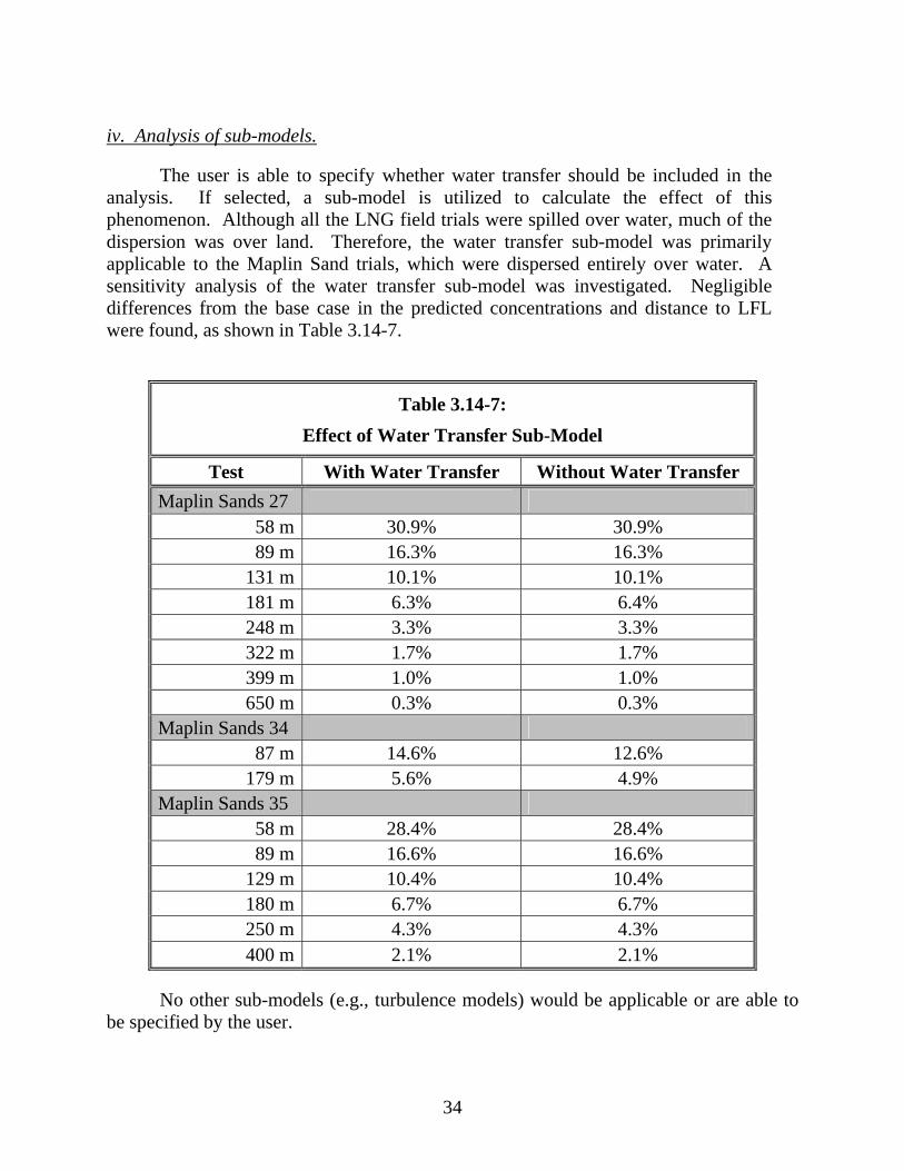
iv. Analysis of sub-models.
The user is able to specify whether water transfer should be included in the analysis. If selected, a sub-model is utilized to calculate the effect of this phenomenon. Although all the LNG field trials were spilled over water, much of the dispersion was over land. Therefore, the water transfer sub-model was primarily applicable to the Maplin Sand trials, which were dispersed entirely over water. A sensitivity analysis of the water transfer sub-model was investigated. Negligible differences from the base case in the predicted concentrations and distance to LFL were found, as shown in Table 3.14-7.
Table 3.14-7:
Effect of Water Transfer Sub-Model
Test With Water Transfer Without Water Transfer
Maplin Sands 27 58 m 30.9% 30.9% 89 m 16.3% 16.3%
131 m 10.1% 10.1% 181 m 6.3% 6.4% 248 m 3.3% 3.3% 322 m 1.7% 1.7% 399 m 1.0% 1.0% 650 m 0.3% 0.3%
Maplin Sands 34 87 m 14.6% 12.6%
179 m 5.6% 4.9% Maplin Sands 35
58 m 28.4% 28.4% 89 m 16.6% 16.6%
129 m 10.4% 10.4% 180 m 6.7% 6.7% 250 m 4.3% 4.3% 400 m 2.1% 2.1%
No other sub-models (e.g., turbulence models) would be applicable or are able to be specified by the user.
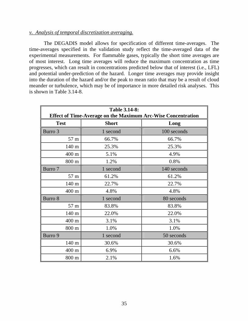
35
v. Analysis of temporal discretization averaging.
The DEGADIS model allows for specification of different time-averages. The time-averages specified in the validation study reflect the time-averaged data of the experimental measurements. For flammable gases, typically the short time averages are of most interest. Long time averages will reduce the maximum concentration as time progresses, which can result in concentrations predicted below that of interest (i.e., LFL) and potential under-prediction of the hazard. Longer time averages may provide insight into the duration of the hazard and/or the peak to mean ratio that may be a result of cloud meander or turbulence, which may be of importance in more detailed risk analyses. This is shown in Table 3.14-8.
Table 3.14-8:
Effect of Time-Average on the Maximum Arc-Wise Concentration
Test Short Long
Burro 3 1 second 100 seconds
57 m 66.7% 66.7%
140 m 25.3% 25.3%
400 m 5.1% 4.9%
800 m 1.2% 0.8%
Burro 7 1 second 140 seconds
57 m 61.2% 61.2%
140 m 22.7% 22.7%
400 m 4.8% 4.8%
Burro 8 1 second 80 seconds
57 m 83.8% 83.8%
140 m 22.0% 22.0%
400 m 3.1% 3.1%
800 m 1.0% 1.0%
Burro 9 1 second 50 seconds
140 m 30.6% 30.6%
400 m 6.9% 6.6%
800 m 2.1% 1.6%

36
Table 3.14-8 (cont’d): Effect of Time-Average on the Maximum Arc-Wise Concentration
Test Short Long
Coyote 3 1 second 50 seconds
140 m 23.9% 23.9%
200 m 14.6% 14.6%
300 m 7.9% 7.8%
400 m 4.9% 4.3%
500 m 3.0% 2.4%
Coyote 5 1 second 90 seconds
140 m 19.6% 19.5%
200 m 13.4% 12.7%
300 m 7.5% 5.3%
400 m 4.9% 2.5%
500 m 3.3% 1.5%
Coyote 6 1 second 70 seconds
140 m 21.6% 21.6%
200 m 14.3% 14.3%
300 m 9.2% 9.2%
400 m 6.1% 6.1%
The maximum arc-wise concentrations are not greatly affected by time averaging, but will generally reduce the concentration. Longer time averages with respect to spill duration, higher turbulence, and higher wind speeds exhibit a greater reduction in concentrations (especially in the far field). The lower concentration may be a result of a lesser hazard duration and/or higher peak to mean ratio from turbulence and/or cloud meander. This reduction in concentration between time averaging can be seen in Coyote 5 where high wind speeds (>10 m/s) and neutral atmospheric stability were present.
The time-averaging in DEGADIS is primarily to take into account cloud meander and will increase gas concentrations farther from the centerline (via the parameterization of horizontal turbulence), while the time-averaging in experimental data will primarily reduce gas concentrations. Therefore, time-averaging has a relatively larger impact on cloud widths than centerline concentration, as shown in Table 3.14-9.

37
Table 3.14-9: Effect of Time-Average on the Plume Width
Test Short Long
Burro 3 1 second 100 seconds
57 m 16.4% 17.0%
140 m 9.3% 12.4%
800 m 17.3% 27.5%
Burro 7 1 second 140 seconds
57 m 11.2% 11.1%
140 m 15.5% 16.7%
400 m 14.7% 17.4%
Burro 8 1 second 80 seconds
57 m 29.0% 28.9%
140 m 40.3% 39.2%
400 m 44.1% 42.8%
800 m 40.5% 39.4%
Burro 9 1 second 50 seconds
140 m 19.5% 27.7%
400 m 35.1% 36.2%
800 m 39.7% 47.6%
Coyote 3 1 second 140 seconds
140 m 19.7% 36.8%
200 m 16.2% 32.7%
400 m 25.7% 57.3%
Coyote 5 1 second 80 seconds
140 m 13.6% 13.7%
200 m 20.1% 20.9%
300 m 25.1% 27.7%
400 m 28.9% 34.4%
500 m 44.2% 57.5%
Coyote 6 1 second 50 seconds
140 m 22.7% 24.2%
200 m 23.6% 24.8%
300 m 23.6% 23.5%
400 m 26.6% 26.8%

38
vi. Analysis of spatial discretization averaging and grid resolution.
As use of a computational mesh is not related to DEGADIS, this section is not applicable.
vii. Analysis of geometrical representation for sloped and obstructed cases.
Sloped terrain and obstructions cannot be modeled with DEGADIS. Therefore, this analysis is not applicable.
3.14.2 Uncertainty Analysis of Model Output
This series of uncertainty analyses addresses model uncertainty due to uncertainty in the output used for evaluation.
i. Analysis of spatial output.
The DEGADIS model outputs concentrations at specific downwind distance intervals that do not always coincide with the experimental sensor locations. Therefore, interpolation of concentrations between downwind distances is often required to determine the concentration at the reflective experimental sensor location. The error associated with the interpolation is dependant on the model’s output with respect to the sensor location. Most often there are not large differences between the interpolation points from a model’s output with respect to the sensor locations and therefore this uncertainty is regarded as being inconsequential.
The determination of the distance to the LFL (taken as 5% for methane) requires interpolation or extrapolation of the experimental data and the model output. The experimental uncertainty associated with the interpolation and extrapolation is dependant on the distance between sensor locations relative to the distance to the LFL concentration. Since there is the potential for large gaps when interpolating and extrapolating the distance to the LFL from the experiments, there is the potential for a greater amount of uncertainty when determining the distance to the LFL for the experiments.
Linear, logarithmic-logarithmic (log-log) and power growth interpolation and extrapolation methodologies have been evaluated to determine the effect on the predicted results. Log-log interpolation of concentration and distance is generally more accepted for unobstructed dispersion compared to other methodologies, but it will generally provide less conservative results (i.e., shorter distances to LFL) and has the potential to under-predict the distances to the LFL. Linear interpolation will generally over-predict concentrations and was used in the Burro Series Report, but linear extrapolation will generally under-predict concentrations (Koopman et al., 1982a) (Koopman et al., 1982b). Linear interpolation and extrapolation also has the potential for higher uncertainties compared to the other methodologies. Power-growth interpolation tends to produce results in between linear and log-log interpolation.

39
In an attempt to “match” the uncertainty between the interpolation and extrapolation of the experimental data with the interpolation and extrapolation of the model output data, the distance to the LFL is interpolated and extrapolated using the sensor locations only. A more refined distance to the LFL from linear interpolation of the more detailed model spatial output is also evaluated to provide a better prediction of the distance to the LFL and an indication of the potential uncertainty from the interpolation and extrapolation methodologies using the experimental sensor locations.
For comparative reasons, the results among the three interpolation and extrapolation methodologies is provided in Table 3.14-10.
Table 3.14-10:
Comparison of Interpolation / Extrapolation Methodologies: Experiment Results
Test
Linearly interpolated/ extrapolated
distance to the LFL
Power growth interpolated/ extrapolated
distance to the LFL
Log-log interpolated/ extrapolated
distance to the LFL
Maplin Sands 27 167m 165 m 158 m Maplin Sands 34 199 m 209 m 241 m Maplin Sands 35 190 m 188 m 187 m Burro 3 268 m 235 m 183 m Burro 7 309 m 276 m 256 m Burro 8 385 m 377 m 356 m Burro 9 361 m 341 m 315 m Coyote 3 212 m 210 m 207 m Coyote 5 277 m 274 m 267 m Coyote 6 281 m 278 m 271 m Falcon 1 293 m 312 m 371 m Falcon 3 280 m 292 m 315 m Falcon 4 6 m 31 m 34 m
As expected for the unobstructed experiments, the linear interpolation provided the most conservative (i.e., farthest distances to the LFL) followed by the power growth interpolation and then the log-log interpolation. Note that the Falcon tests, which contain obstructions in the flow field and had to be extrapolated, follow the opposite trend, as shown in Table 3.14-10.
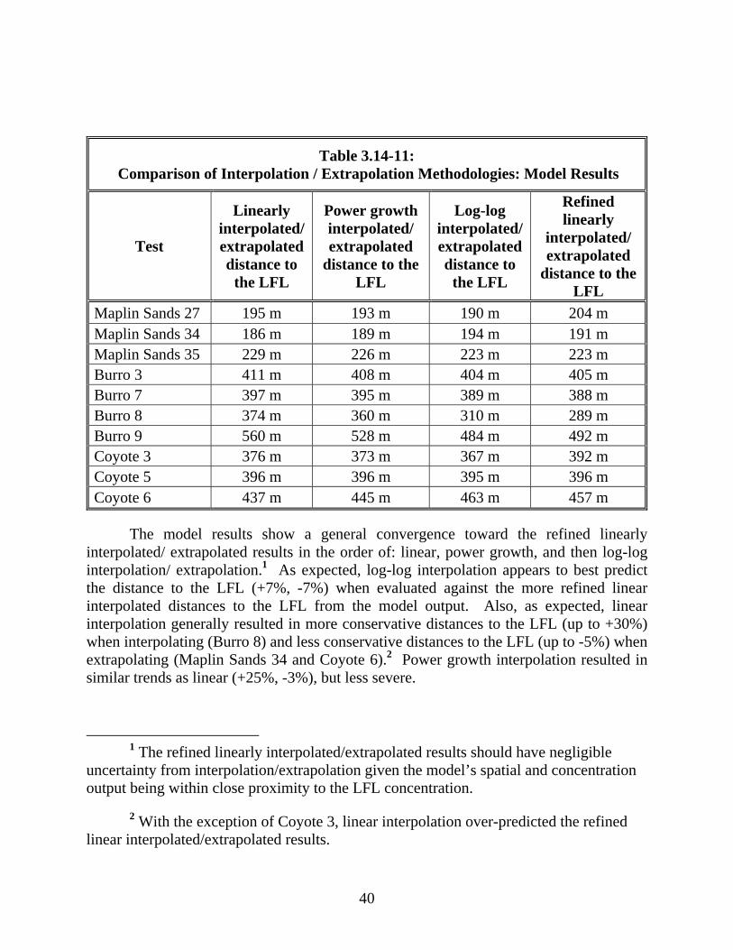
40
Table 3.14-11: Comparison of Interpolation / Extrapolation Methodologies: Model Results
Test
Linearly interpolated/ extrapolated distance to
the LFL
Power growth interpolated/ extrapolated
distance to the LFL
Log-log interpolated/ extrapolated distance to
the LFL
Refined linearly
interpolated/ extrapolated
distance to the LFL
Maplin Sands 27 195 m 193 m 190 m 204 m Maplin Sands 34 186 m 189 m 194 m 191 m Maplin Sands 35 229 m 226 m 223 m 223 m Burro 3 411 m 408 m 404 m 405 m Burro 7 397 m 395 m 389 m 388 m Burro 8 374 m 360 m 310 m 289 m Burro 9 560 m 528 m 484 m 492 m Coyote 3 376 m 373 m 367 m 392 m Coyote 5 396 m 396 m 395 m 396 m Coyote 6 437 m 445 m 463 m 457 m
The model results show a general convergence toward the refined linearly interpolated/ extrapolated results in the order of: linear, power growth, and then log-log interpolation/ extrapolation.1 As expected, log-log interpolation appears to best predict the distance to the LFL (+7%, -7%) when evaluated against the more refined linear interpolated distances to the LFL from the model output. Also, as expected, linear interpolation generally resulted in more conservative distances to the LFL (up to +30%) when interpolating (Burro 8) and less conservative distances to the LFL (up to -5%) when extrapolating (Maplin Sands 34 and Coyote 6).2 Power growth interpolation resulted in similar trends as linear (+25%, -3%), but less severe.
1 The refined linearly interpolated/extrapolated results should have negligible
uncertainty from interpolation/extrapolation given the model’s spatial and concentration output being within close proximity to the LFL concentration.
2 With the exception of Coyote 3, linear interpolation over-predicted the refined linear interpolated/extrapolated results.
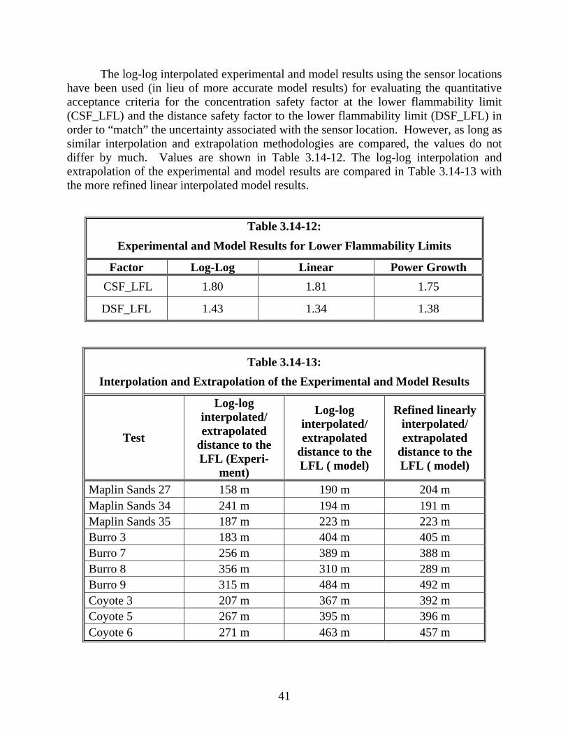
41
The log-log interpolated experimental and model results using the sensor locations have been used (in lieu of more accurate model results) for evaluating the quantitative acceptance criteria for the concentration safety factor at the lower flammability limit (CSF_LFL) and the distance safety factor to the lower flammability limit (DSF_LFL) in order to “match” the uncertainty associated with the sensor location. However, as long as similar interpolation and extrapolation methodologies are compared, the values do not differ by much. Values are shown in Table 3.14-12. The log-log interpolation and extrapolation of the experimental and model results are compared in Table 3.14-13 with the more refined linear interpolated model results.
Table 3.14-12:
Experimental and Model Results for Lower Flammability Limits
Factor Log-Log Linear Power Growth
CSF_LFL 1.80 1.81 1.75
DSF_LFL 1.43 1.34 1.38
Table 3.14-13:
Interpolation and Extrapolation of the Experimental and Model Results
Test
Log-log interpolated/ extrapolated
distance to the LFL (Experi-
ment)
Log-log interpolated/ extrapolated
distance to the LFL ( model)
Refined linearly interpolated/ extrapolated
distance to the LFL ( model)
Maplin Sands 27 158 m 190 m 204 m Maplin Sands 34 241 m 194 m 191 m Maplin Sands 35 187 m 223 m 223 m Burro 3 183 m 404 m 405 m Burro 7 256 m 389 m 388 m Burro 8 356 m 310 m 289 m Burro 9 315 m 484 m 492 m Coyote 3 207 m 367 m 392 m Coyote 5 267 m 395 m 396 m Coyote 6 271 m 463 m 457 m

42
In addition, the model assumes a top-hat and Gaussian concentration profile in the cross-wise direction. Maximum concentrations are based upon the maximum concentration predicted by the model, which corresponds to the centerline concentration predicted in the integral model. However, the maximum concentration may not always be captured by the experiment or occur along the centerline. This will cause the model to generally over-predict experimental data where the actual maximum concentration was not captured by the sensors in the experiment. Cloud meandering during the experiments may reduce this over-prediction, but for many experiments the wind direction was fairly steady and meandering may not be significant.
The effect of this has been analyzed to some extent by evaluating the point-wise data that accounts for the offset between the vapor cloud centerline and the sensor that received the maximum concentration for the test. However, experimental data shows that maximum concentrations may not always exist along the centerline, which makes quantifying this effect more complex.
ii. Analysis of temporal output.
The DEGADIS model outputs concentrations at specific time intervals. The maximum concentration produced over the outputted time periods were utilized, and therefore no interpolation or extrapolations were utilized. This is not considered to be a large source of uncertainty.
3.14.3 Uncertainty Analysis of Experimental Data
This uncertainty analysis addresses experimental uncertainty due to uncertainty in the sensor measurement of gas concentration. The experimental uncertainty due to uncertainty in the sensor measurement was taken into account based upon the 90% confidence levels and uncertainties provided in the respective data series reports (Koopmanet al., 1982a) (Koopman et al., 1982b) (Goldwire et al., 1983a) (Goldwire et al., 1983b). This is shown in Table 3.14-14.

43
Table 3.14-14: Uncertainty in the Sensor Measurement of Gas Concentration
Test Measured (vol%) - (vol%) + (%vol)
Maplin Sands 27 Short Time Avg. 58 m 16.9 5.3 5.2 89 m 12.3 4.0 3.8
129 m 9.5 3.2 3.1 181 m 3.3 1.4 1.5 248 m 3.0 1.3 1.4 322 m 2.4 1.1 1.2 399 m 2.9 1.3 1.4 525 m - - - 650 m 0.1 0.1 0.6
Maplin Sands 34 Short Time Avg. 89 m 18.1 5.6 5.6
180 m 7.3 2.6 2.5
Maplin Sands 35 Short Time Avg. 58 m 13.3 4.3 4.1 89 m 9.9 3.4 3.2
129 m 7.9 2.8 2.7 180 m 5.3 2.0 2.0 250 m 3.4 1.4 1.5 400 m 2.2 1.1 1.2

44
Table 3.14-14 (cont’d): Uncertainty in the Sensor Measurement of Gas Concentration
Test Measured
(vol%) -
(vol%)+
(%vol) Measured
(vol%) -
(vol%) +
(%vol)
Burro 3 Short Time Avg. Long Time Avg.
57 m 28.2 1.6 1.6 8.5 0.5 0.5
140 m 9.0 0.5 0.5 6.4 0.4 0.4
400 m 1.2 0.4 0.4 0.7 0.2 0.2
800 m 0.9 0.3 0.3 0.9 0.3 0.3
Burro 7 Short Time Avg. Long Time Avg.
57 m 17.9 9.0 9.0 14.8 7.4 7.4
140 m 7.3 3.7 3.7 4.5 2.3 2.3
400 m 3.9 1.2 1.2 2.3 0.7 0.7
Burro 8 Short Time Avg. Long Time Avg.
57 m 55.9 3.1 3.1 31.0 1.7 1.7
140 m 18.1 9.1 9.1 16.4 8.2 8.2
400 m 6.1 1.8 1.8 5.4 1.6 1.6
800 m 2.1 0.6 0.6 2.1 0.6 0.6
Burro 9 Short Time Avg. Long Time Avg.
140 m 10.6 0.6 0.6 6.6 0.4 0.4
400 m 5.1 2.6 2.6 2.9 1.5 1.5
800 m 2.2 0.7 0.7 1.4 0.4 0.4

45
Table 3.14-14 (cont’d): Uncertainty in the Sensor Measurement of Gas Concentration
Test Measured
(vol%) -
(vol%)+
(%vol)Measured
(vol%) -
(vol%) +
(%vol)
Coyote 3 Short Time Avg. Long Time Avg.
140m 10.7 0.6 0.6 5.4 0.3 0.3
200m 5.4 0.3 0.3 2.9 0.2 0.2
300m 1.9 0.2 0.2 0.9 0.1 0.1
400m 2.0 0.2 0.2 0.9 0.1 0.1
500m 0.4 0.1 0.1 0.1 0.0 0.0
Coyote 5 Short Time Avg. Long Time Avg.
140m 11.5 0.6 0.6 4.2 0.2 0.2
200m 8.1 0.4 0.4 2.5 0.1 0.1
300m 4.1 0.4 0.4 1.1 0.1 0.1
400m 2.3 0.1 0.1 0.8 0.0 0.0
500m 1.8 0.5 0.5 0.5 0.2 0.2
Coyote 6 Short Time Avg. Long Time Avg.
140m 12.7 0.7 0.7 8.4 0.5 0.5
200m 8.5 0.5 0.5 5.1 0.3 0.3
300m 4.2 0.4 0.4 2.2 0.2 0.2
400m 3.3 0.2 0.2 2.0 0.1 0.1
500m 2.6 0.8 0.8 1.9 0.6 0.6
Experimental uncertainty due to the sampling time, time averaging, spatial/volumetric averaging, cloud meander, and other errors or uncertainties associated with the experiment were not required to be quantified by the Advisory Bulletin; however, examination of all sensor data provided additional insight into uncertainty associated with the maximum concentrations recorded in the MEP. These uncertainties were noted in the validation database for each sensor and quantified, where possible. Where it was possible to estimate the uncertainty, it was included as part of the experimental uncertainty. Several qualitative examples are provided for the Burro series:

46
In some tests the IST sensors became saturated with high concentrations (~18%) and became “pegged” out. Burro 3 data indicates that the 57 m arc may not be a good indication of the maximum concentration because there was no sensor that coincided with the “centerline” of cloud for this test and there was minimal fluctuation in wind direction. Therefore, the maximum concentration is based on sensors 14 m from the vapor cloud “centerline.”
Burro 7 data indicates that early in the test the wind direction may have prevented the vapor cloud from dispersing over the sensor array at the 57 m arc. This may have prevented the sensors from capturing the actual maximum concentration.
Burro 8 data indicates bifurcation of the vapor cloud.
Burro 9 data indicates that a large rapid phase transition occurred during the experiments that may have affected the accuracy of the sensor array at the 57 m arc. In addition, the lowest positioned sensor at the 57 m arc was not operable and would have likely experienced the maximum concentration due to its low elevation.
3.14.4 Uncertainty Analysis Results
Graphical depictions of the predicted and measured gas concentration values for each experiment, with indication of the experimental and model uncertainty, are shown in the accompanying validation database.
3.14.5 Additional Specific Performance Measures
Calculation of the specific performance measures identified in the MEP and the Advisory Bulletin are shown in the accompanying validation database.
3.14.6 Individual Specific Performance Measures
Calculation of specific performance measures, as identified in the MEP and the Advisory Bulletin, for each experiment and data point, as well as the the average of all experiments, is shown in the accompanying validation database.
3.14.7 Model Input/Output Results
A tabulation of all simulations, including all specified input parameters and calculated outputs is provided in the accompanying validation database.

47
3.14.8 Specific Performance Measures Results
A tabulation of all calculated specific performance measures is provided in the accompanying validation database.
3.14.9 Input and Output Files
All relevant input and output files used in preparation of this document are included in the accompanying validation database.

48
4.0 CONCLUSIONS
4.1 SCIENTIFIC ASSESSMENT
DEGADIS is an integral model developed by Spicer and Havens derived from the HEGADAS mathematical model published by Colenbrander et al at Shell (1980). DEGADIS solves for the concentration, advecting downwind, with parameterized turbulent diffusion coefficients and top entrainment velocity. DEGADIS also solves for the temperature of the vapor, and includes heat transfer from the air, including relative humidity, and from the ground.
DEGADIS solves ordinary differential equations using the Runge-Kutta method using a variable step that is 4th order accurate. Although this methodology can be considered a source of uncertainty, it is not expected to be a large source of uncertainty for the results.
DEGADIS does not include a source term model to simulate any characteristics associated with the release, such as flow rates associated with the release, flashing of superheated liquids upon a release, the formation, vaporization, or rainout of aerosol droplets upon a release, or the formation, vaporization, or spreading of a liquid pool upon a release. DEGADIS requires the specification of a gaseous source term from the user.
DEGADIS is limited to handling a low-momentum source term where the diameter and vaporization rate are specified as a function of time, or a high momentum jet source term where the jet diameter, release rate, elevation, and duration are specified. DEGADIS is limited to a single source term. DEGADIS cannot be used to model multiple source terms (i.e., flashing and jetting sources that rainout to a pool, multiple release locations).
For an area source term, DEGADIS assumes the source is vertically oriented circular geometry with no momentum. Therefore, for area source terms, DEGADIS is limited to vertically oriented, low-momentum releases with regular geometries, such as vapors emanating from circular or rectangular sources (i.e., liquid pools or sumps). For area source terms for DEGADIS cannot be used for high-momentum releases (i.e. pressurized releases, flashing, jetting), or for releases that result in the emanation of vapors from irregular or high aspect ratio sources (i.e., trenches, or irregular liquid pools).
For a jet source term, DEGADIS assumes the source is vertically oriented circular geometry that accounts for turbulence associated with the momentum of the release, but does not account for turbulence associated with a release reaching grade or impinging onto a surface. Therefore, for jet source terms, DEGADIS is limited to vertically oriented releases that do not reach grade (i.e., vent stack releases that do not reach grade, flashing from vertically oriented piping, and gaseous releases from vertically oriented piping that do not reach grade). The DEGADIS jet plume model cannot be used for

49
horizontally oriented source terms or releases that may reach grade level or impinge onto a surface (i.e., flashing from horizontally oriented piping, any release that reaches grade).
DEGADIS is limited to simulating steady state wind profiles. DEGADIS cannot model transient wind speed or direction. Assuming a steady state wind speed and direction is often sufficient for hazard analyses, but can pose limitation in validation against experimental data where varying wind speed and direction may affect the experimental results. The selection of wind direction is not pertinent or possible in DEGADIS, since it assumes a circular source term where the dispersion will be axi-symmetric. Assuming a steady wind direction will generally produce higher concentrations, because there would be less cloud meander and turbulent mixing caused from the change in wind direction. Assuming lower wind speeds will generally result in higher downwind concentrations and assuming a higher wind speed will generally result in lower downwind concentrations. DEGADIS generally produces the highest downwind concentrations at 2 m/s. DEGADIS should be specified with the lower wind speed that is reflective of the area or with wind speeds of 2 m/s to produce conservative results. For most applications pertinent to this study, DEGADIS will be used in accordance with 49 C.F.R. § 193.2059, which specifies the lowest wind speed that occurs 90% of time for the area or 2 m/s. Steady state wind speed and direction is not expected to be a large limitation of the model.
DEGADIS cannot account for sloped or varying terrain. Sloped or varying terrain will affect the gravity spreading of a dense gas release. For dense gas releases, such as LNG vapor, concentrations in the far field may be under-predicted along downward slopes and concentrations in the far field may be over-predicted along upward slopes. Correspondingly, cross-wise concentrations and cloud widths in the far field may be over-predicted for downward slopes and cross-wise concentrations and cloud widths in the far field may be under-predicted for upward slopes. On the contrary, gas may accumulate against an upward slope causing the model to under-predict gas concentrations and over-predict cross-wise concentrations and cloud widths in the near field or traverse along a downward slope causing the model to over-predict gas concentrations and under-predict cross-wise concentrations and cloud widths in the near field. DEGADIS was not validated against sloped terrain tests, since it is not designed to simulate those scenarios. Therefore, DEGADIS cannot be used to model dispersion along slopes or varying terrain.
DEGADIS is limited to the specification of a single surface roughness. DEGADIS cannot account for terrain with varying surface roughness length. Assuming a uniform surface roughness is often sufficient. Assuming a higher surface roughness will generally result in lower downwind concentrations and assuming a lower surface roughness will generally result in higher downwind concentrations. DEGADIS should be specified with the lowest surface roughness that is reflective of the area to produce conservative results. For most applications pertinent to this study, DEGADIS will be
50
used in accordance with 49 C.F.R. § 193.2059, which specifies the surface roughness of 0.03 m, so this is not expected to be a large limitation of the model.
DEGADIS does not explicitly model turbulence generated in the flow field from obstructions and cannot take into account the change in flow field around obstructions that are relatively larger than the vapor cloud. For most instances, downwind concentrations assuming unobstructed terrain will be over-predictive since less turbulence, and subsequent mixing, would be generated in the flow field and no obstructions would restrict the movement of the dispersing vapor. However, there are instances where downwind concentrations could be under-predictive due to wind channeling effects (Melton & Cornwell, 2009, Gavelli 2011). Wind channeling may occur between adjacent LNG storage tanks, buildings, or large structures, which may result in the model being under-predictive for concentrations. Therefore, DEGADIS cannot be used to model releases that may disperse between large adjacent structures.
DEGADIS accounts for atmospheric turbulent mixing and dilution through the use of empirically derived turbulent mixing coefficients and top entrainment. DEGADIS does not explicitly calculate stochastic fluctuations due to turbulence in the flow field. Stochastic fluctuations in concentration can result in concentrations higher or lower than predicted. Therefore, it is recommended that concentrations should be provided with a safety factor of 2 for the LFL to account for estimated peak to mean turbulent fluctuations (MER Section 2.3.5). In addition, for area source terms, DEGADIS assumes a no-momentum release and does not take into account possible turbulence generated by the release. Therefore, for area source terms, DEGADIS cannot be used for high-momentum releases (i.e. pressurized releases, flashing, jetting). Assuming no turbulence at a low-momentum source (i.e., turbulence generated at the surface of a boiling pool) will generally result in lower downwind concentrations because there is less turbulent mixing. For jet source terms, DEGADIS accounts for turbulent mixing from the jet release, but does not account for turbulence associated with impingement of a jet or with a dense vapor cloud reaching grade. Therefore, for jet source terms, DEGADIS cannot be used for releases that may reach grade level or impinge onto a surface (i.e., flashing from horizontally oriented piping, any release that reaches grade).
4.2 VERIFICATION
The verification of the model has been limited to accuracy of the conservation relations (e.g. conservation of mass), and has not been documented. The model predates the European Commission’s Model Evaluation Group publications and many other software quality assurance publications, certifications (International Organization for Standardization: Standard 9000 - Quality Management), or standards. The software is not proprietary and its executable and source code files are freely available to the public, which makes it possible for users to modify the source code and recompile the executable, making quality control unmanageable. To address the lack of quality

51
assurance / quality control possible with DEGADIS, it is encouraged that simulations be verified by an independent party or agency.
4.3 VALIDATION
As discussed in Section 4.1, “Scientific Assessment,” the DEGADIS model is limited to dispersion over unobstructed level terrain specified by the user. Therefore, the current validation study is limited to the following trials:
LNG Field Trials: Maplin Sands 27, 34, 35; Burro 3, 7, 8, 9; Coyote 3, 5, 6;
Other Field Trials: Thorney Island 45, 47;
Wind Tunnel Experiments: CHRC A; BA-Hamburg DA0120 (Unobstructed), DAT223 (Unobstructed 2); and BA-TNO TUV01, FLS.
DEGADIS met most of the MEP quantitative acceptance criteria for short time averages with the exception of mean relative bias, MRB, and mean relative square error, MRSE, as shown in Table 2.2-1. As shown in Figure 4.3-1 and supported by the statistical performance measure values, DEGADIS is generally over-predictive, but exhibits a large degree of scatter and only about half of its predictions are within a factor of 2. However, the MEP specific performance measures and quantitative acceptance criteria are based on an average of all the trials, which can be misleading. Therefore, it was recognized in the Advisory Bulletin that the approval or disapproval of a model should not be contingent only on the average of the experiments meeting the MEP quantitative acceptance criteria. Careful examination of all the sensor data and trends must be considered in concert with the MEP quantitative acceptance criteria. As shown in Table 2.2-2, these trends provide additional insight into the model performance against subsets of data.
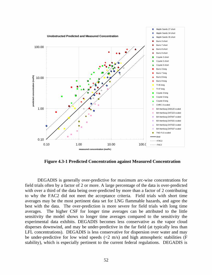
52
Unobstructed Predicted and Measured Concentration
0.10
1.00
10.00
100.00
0.10 1.00 10.00 100.00
measured concentration (mol%)
pre
dic
ted
co
nc
en
tra
tio
n (
mo
l%)
Maplin Sands 27 short
Maplin Sands 34 short
Maplin Sands 35 short
Burro 3 short
Burro 7 short
Burro 8 short
Burro 9 short
Coyote 3 short
Coyote 5 short
Coyote 6 short
Burro 3 long
Burro 7 long
Burro 8 long
Burro 9 long
TI 45 long
TI 47 long
Coyote 3 long
Coyote 5 long
Coyote 6 long
CHRC A scaled
BA Hamburg DA0120 scaled
BA Hamburg DAT223 scaled
BA Hamburg DAT647 scaled
BA Hamburg DAT631 scaled
BA Hamburg DAT632 scaled
BA Hamburg DAT637 scaled
TNO FLS scaled
ideal
+FAC2
-FAC2
Figure 4.3-1 Predicted Concentration against Measured Concentration
DEGADIS is generally over-predictive for maximum arc-wise concentrations for field trials often by a factor of 2 or more. A large percentage of the data is over-predicted with over a third of the data being over-predicted by more than a factor of 2 contributing to why the FAC2 did not meet the acceptance criteria. Field trials with short time averages may be the most pertinent data set for LNG flammable hazards, and agree the best with the data. The over-prediction is more severe for field trials with long time averages. The higher CSF for longer time averages can be attributed to the little sensitivity the model shows to longer time averages compared to the sensitivity the experimental data exhibits. DEGADIS becomes less conservative as the vapor cloud disperses downwind, and may be under-predictive in the far field (at typically less than LFL concentrations). DEGADIS is less conservative for dispersion over water and may be under-predictive for low wind speeds (<2 m/s) and high atmospheric stabilities (F stability), which is especially pertinent to the current federal regulations. DEGADIS is

53
generally under-predictive for wind tunnel experiments often by a factor of 2 or more. All wind tunnel data was under-predicted with the majority of the data being under-predicted by more than a factor of 2 contributing to the FAC2 not meeting the acceptance criteria. Similar to the field trials, DEGADIS becomes less conservative as the vapor disperses downwind, and may be under-predictive in the far field at lower concentrations. DEGADIS performs better for the CHRC test, which was designed to be used as a scale model for LNG dispersion.
DEGADIS compares much better with maximum gas concentration distances, and meets nearly all the acceptance criteria. DEGADIS shows similar trends for field trials and wind-tunnel tests. DEGADIS generally over-predicts the distance to a given concentration for field trials by approximately a factor of 1.5, and under-predicts wind-tunnel tests by approximately a factor of 1.5. The relatively better agreement is because large concentration differences may manifest themselves as much smaller differences in distance.
DEGADIS generally over-predicts point-wise gas concentrations that are located at an angle corresponding to the wind direction where the maximum arc-wise concentration often occurred, and under-predicts point-wise gas concentrations that are located farther from the “centerline”. The under-prediction of concentrations farther from the “centerline” is much more drastic than the over-prediction near the “centerline,” which results in an average under-prediction and a high degree of scatter. In addition, DEGADIS generally seems to under-predict short time averages and over-predict long time averages with a difference of a factor of 2 or more between them.
Similarly to maximum gas concentration distances, DEGADIS compares much better with cloud widths. However, DEGADIS generally under-predicts the cloud width by a factor of 1.5. Cloud widths are also less influenced by large concentration differences, which may manifest themselves as much smaller differences in cloud widths. Cloud widths are not a particular concern with 49 CFR Part 193, but may cause under prediction of the hazard footprint, which can affect risk analyses or performance based design of gas detectors.
DEGADIS may be less conservative or under-predictive for maximum arc-wise concentrations for field trials with low wind speed and high atmospheric stabilities, a particular concern for 49 CFR Part 193. Although the field trials are most applicable to the scenarios considered under the Part 193 regulations and generally show over-prediction, there are a number of uncertainties that indicate potential under-prediction by a factor of 2. Until these uncertainties are resolved, it is recommended that a safety factor of 2 be used when evaluating predicted maximum arc-wise concentrations from DEGADIS. Alternatively, a distance safety factor of 2 may be used.

54
4.4 SENSITIVITY ANALYSES
The sensitivity analyses for DEGADIS indicates little sensitivity to the pool spread velocity, vaporization rate, and pool diameter for spills over water. However, all the LNG field trial releases were conducted over water and the associated source terms will be different than those used on land. For spills over water with significant depth, the heat transfer to the pool is generally considered constant due to convective motion of the water. For spills over land, the heat transfer to the pool is generally considered to be transient due to conductive cooling of the substrate. Pressurized releases may further deviate from the more idealized source term for spills over water. Therefore for spills over land and pressurized releases, it is recommended that the source term is evaluated before usage.
Longer time averages result in slightly lower maximum arc-wise gas concentrations, and significantly higher maximum point-wise concentrations away from the centerline. The maximum point-wise gas concentrations are affected more significantly because DEGADIS parameterizes its horizontal turbulence coefficients based on time averaging to take into account cloud meander. In contrast, longer time averages of experimental data will only result in lesser concentrations. Therefore, comparison with longer experimental time averages may cause the model to appear more conservative than it actually is. Short time averages are more appropriate for the hazard and should be used when predicting flammable vapor centerline concentrations.
Many of the trials did not have wind speeds that differed by more than 10%. For trials that did not have wind speeds that differed by more than 10%, lower wind speeds generally produced higher downwind concentrations and dispersion distances, and higher wind speeds produced lower downwind concentrations and dispersion distances. The exceptions were Burro 8 where very low wind speeds (< 2 m/s) occurred and Maplin Sands 34 where very high wind speeds (> 8 m/s) occurred.
The surface roughness values have the largest uncertainties. The values specified in the MEP are generally low and result in higher concentrations and longer dispersion distances to the LFL, which may cause the model to appear more conservative than it actually is. However, even with less conservative parameters, the model still generally over-predicts concentrations. If the surface roughness is prescribed, such as the case in 49 C.F.R. § 193.2059, it should be made sure that the surface roughness is appropriate based on photographic documentation, visual observations, or meteorological data representative of the site. For LNG releases that disperse over land, a surface roughness of 0.03 may be justified, however, for LNG facilities that release over water, such as for offshore facilities or marine loading/unloading platforms that are situated away from the shoreline, a lower surface roughness may be more appropriate.

55
Lower atmospheric stabilities generally produced lower downwind concentrations and dispersion distances, and higher atmospheric stabilities produced higher downwind concentrations and dispersion distances. Where the surface roughness uncertainty was low, the atmospheric stability often formed the upper or lower bound of the predictions.
Ambient temperature and surface temperature had little fluctuation, and therefore no sensitivity cases were run. However, higher ambient temperatures and surface temperatures should generally produce lower gas concentrations and downwind dispersion distances.
None of the trials had ambient pressures that differed by more than 10% from atmospheric pressure, but in order to test the sensitivity, Burro 7, which had the lowest ambient pressure was tested. Higher ambient pressure showed slightly lower concentrations and downwind dispersion distances.
Many of the trials did not have ambient relative humidity that differed by more than 10%, but some of the values disagreed with those reported in the original data series reports. For trials that did not have ambient relative humidity that differed, lower ambient relative humidity generally produced higher gas concentrations in the near field, but lower gas concentrations in the far field, and vice-versa.
The water transfer submodel showed negligible differences when included in the predicted concentrations and distance to LFL.
The molecular weight specified in the MEP reflects the composition of the LNG and does not take into account preferential boiloff. The lower molecular weight of methane results in higher concentrations and longer dispersion distances to the LFL. However, even with less conservative parameters, the model still generally over-predicts concentrations. The molecular weight of methane is recommended to be used to account for potential preferential boiloff and conservatism.
Overall, the sensitivity analysis showed concentrations may differ by more than a factor of four and downwind dispersion distances to the LFL may differ by up to a factor of two, dependant on the uncertainty in the user input and sensitivity to that input.
4.5 MODEL SUITABILITY AND LIMITATIONS
DEGADIS requires a source term to be inputted into the model. The specification of the source term is a key parameter in determining the gas concentrations and dispersion distances, but is not examined under the MEP or the Advisory Bulletin. The suitability of the source term model must be reviewed before being used in Part 193 calculations.

56
DEGADIS may be used to model the maximum arc-wise concentration for:
Dispersion from circularly shaped LNG pools;
Dispersion from LNG pools with low-aspect ratios, including most impoundments;
Dispersion from vertically oriented releases that do not reach grade, including releases from flashing, venting, vent stacks, and pressure relief discharge; or
Dispersion over flat or upward sloped terrain.
DEGADIS may not be appropriate to be used to model the maximum arc-wise concentration for:
Dispersion from irregularly shaped LNG pools
Dispersion from LNG pools with high-aspect ratios, including some impoundments and nearly all trenches;
Dispersion from vertically oriented releases that reach grade, including releases from flashing, venting, vent stacks, and pressure relief discharge;
Dispersion from horizontally oriented releases, including flashing, jetting, venting, and pressure relief discharge;
Dispersion from multiple coincident releases, including multiple release locations;
Dispersion over varying or downward sloped terrain; or
Dispersion between large obstructions that may cause wind-channeling.
DEGADIS may not be appropriate to model point-wise concentrations, and may be under-predictive for cloud widths.
The ambient conditions required under 49 CFR § 193.2059 should produce conservative results (i.e. higher downwind gas concentrations and dispersion distances).
DEGADIS should be used with a safety factor of 2 (i.e. ½ LFL) to compensate for uncertainties related to potential turbulent fluctuations, wind tunnel experiment validation results, and low wind speed and high atmospheric stability validation results.

APPENDIX A: SENSITIVITY CASE RESULTS
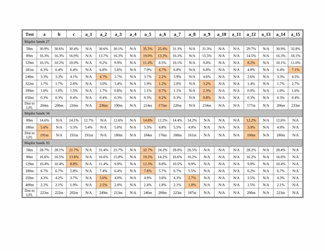
Test a b c a_1 a_2 a_3 a_4 a_5 a_6 a_7 a_8 a_9 a_10 a_11 a_12 a_13 a_14 a_15
Maplin Sands 27
58m 30.9% 30.6% 30.4% N/A 30.6% 30.1% N/A 35.5% 25.4% 31.3% N/A 31.3% N/A N/A 29.7% N/A 30.9% 32.8%
89m 16.3% 16.3% 16.9% N/A 13.7% 16.3% N/A 19.0% 13.3% 16.3% N/A 15.5% N/A N/A 14.5% N/A 16.3% 18.1%
129m 10.1% 10.2% 10.0% N/A 9.2% 9.9% N/A 11.4% 8.5% 10.1% N/A 9.8% N/A N/A 8.2% N/A 10.1% 11.0%
181m 6.3% 6.4% 6.4% N/A 6.8% 5.6% N/A 7.0% 4.7% 6.8% N/A 6.8% N/A N/A 4.8% N/A 6.4% 7.1%
248m 3.3% 3.3% 4.1% N/A 4.7% 2.7% N/A 3.7% 2.2% 3.9% N/A 4.6% N/A N/A 2.6% N/A 3.3% 4.5%
322m 1.7% 1.7% 2.6% N/A 3.0% 1.4% N/A 1.9% 1.2% 2.0% N/A 3.2% N/A N/A 1.4% N/A 1.7% 2.7%
399m 1.0% 1.0% 1.5% N/A 1.7% 0.8% N/A 1.1% 0.7% 1.1% N/A 2.3% N/A N/A 0.9% N/A 1.0% 1.6%
650m 0.3% 0.3% 0.4% N/A 0.4% 0.3% N/A 0.3% 0.2% 0.3% N/A 0.8% N/A N/A 0.3% N/A 0.3% 0.4%
Dist to LFL
204m 206m 216m N/A 236m 190m N/A 214m 175m 220m N/A 234m N/A N/A 177m N/A 206m 233m
Maplin Sands 34
89m 14.6% N/A 14.1% 12.7% N/A 12.6% N/A 14.8% 12.2% 14.4% 14.2% N/A N/A N/A 12.2% N/A 12.6% N/A
180m 5.6% N/A 5.5% 5.4% N/A 5.0% N/A 5.5% 4.8% 5.5% 4.0% N/A N/A N/A 3.9% N/A 4.9% N/A
Dist to LFL
191m N/A 191m 191m N/A 180m N/A 184m 176m 188m 161m N/A N/A N/A 160m N/A 180m N/A
Maplin Sands 35
58m 28.7% 28.1% 21.7% N/A 31.4% 25.7% N/A 32.7% 24.2% 28.0% 26.5% N/A N/A N/A 28.2% N/A 28.4% N/A
89m 16.6% 16.5% 13.6% N/A 16.6% 15.8% N/A 19.5% 14.2% 16.6% 16.2% N/A N/A N/A 16.2% N/A 16.6% N/A
129m 10.4% 10.4% 8.8% N/A 11.4% 9.9% N/A 12.3% 8.8% 10.5% 9.9% N/A N/A N/A 9.9% N/A 10.4% N/A
180m 6.7% 6.7% 5.8% N/A 7.4% 6.4% N/A 7.6% 5.7% 6.7% 5.5% N/A N/A N/A 6.2% N/A 6.7% N/A
250m 4.3% 4.2% 3.7% N/A 5.0% 4.0% N/A 4.9% 3.6% 4.3% 2.7% N/A N/A N/A 3.5% N/A 4.3% N/A
400m 2.1% 2.1% 1.9% N/A 2.5% 2.0% N/A 2.4% 1.8% 2.1% 1.0% N/A N/A N/A 1.5% N/A 2.1% N/A
Dist to LFL
223m 222m 202m N/A 249m 213m N/A 246m 200m 223m 187m N/A N/A N/A 206m N/A 223m N/A

Test a b c a_1 a_2 a_3 a_4 a_5 a_6 a_7 a_8 a_9 a_10 a_11 a_12 a_13 a_14 a_15
Burro 3
57m 66.7% 66.3% 64.4% 66.7% 68.3% 64.5% 67.0% N/A 41.2% N/A N/A 68.0% N/A N/A N/A N/A N/A 68.5%
140m 25.3% 25.2% 25.1% 25.3% 26.0% 24.8% 25.1% N/A 12.2% N/A N/A 26.6% N/A N/A N/A N/A N/A 27.5%
400m 5.1% 5.0% 4.9% 4.9% 5.2% 5.0% 5.1% N/A 2.4% N/A N/A 5.3% N/A N/A N/A N/A N/A 5.5%
800m 1.2% 1.2% 1.6% 0.8% 1.1% 1.3% 1.2% N/A 0.5% N/A N/A 1.8% N/A N/A N/A N/A N/A 1.7%
Dist to LFL
405m 402m 394m 395m 414m 397m 404m N/A 257m N/A N/A 414m N/A N/A N/A N/A N/A 424m
Burro 7
57m 61.2% 60.7% 49.4% 61.2% N/A N/A 61.4% N/A 33.9% 60.9% 60.0% N/A N/A 60.0% 58.9% N/A N/A 64.1%
140m 22.7% 22.4% 2.2% 22.7% N/A N/A 23.2% N/A 11.0% 22.5% 21.4% N/A N/A 21.5% 22.7% N/A N/A 26.7%
400m 4.8% 4.8% 4.4% 4.8% N/A N/A 4.8% N/A 2.4% 4.8% 4.6% N/A N/A 4.6% 4.8% N/A N/A 5.3%
Dist to LFL
388m 387m 368m 388m N/A N/A 390m N/A 242m 388m 381m N/A N/A 374m 386m N/A N/A 414m
Burro 8
57m 83.8% 100% 100% 83.8% 88.3% 89.8% 83.9% N/A 67.2% 85.5% N/A 80.2% N/A N/A N/A N/A N/A 68.9%
140m 22.0% 22.5% 21.0% 22.0% 16.3% 25.1% 21.9% N/A 15.7% 23.1% N/A 21.8% N/A N/A N/A N/A N/A 29.4%
400m 3.1% 2.9% 3.3% 3.1% 2.1% 3.6% 3.1% N/A 3.5% 3.5% N/A 2.9% N/A N/A N/A N/A N/A 5.3%
800m 1.0% 1.0% 1.1% 1.0% 0.7% 1.2% 1.0% N/A 1.3% 1.1% N/A 1.0% N/A N/A N/A N/A N/A 1.5%
Dist to LFL
289m 291m 308m 289m 221m 329m 290m N/A 302m 328m N/A 284m N/A N/A N/A N/A N/A 415m
Burro 9
57m 76.4% 76.1% 73.6% 76.4% N/A N/A 76.5% N/A 45.7% 76.5% N/A 74.9% N/A N/A 76.9% N/A N/A 79.1%
140m 30.6% 29.5% 29.7% 30.6% N/A N/A 31.2% N/A 15.9% 30.8% N/A 30.4% N/A N/A 32.5% N/A N/A 37.5%
400m 6.9% 6.6% 6.3% 6.6% N/A N/A 6.9% N/A 3.4% 6.9% N/A 6.7% N/A N/A 6.6% N/A N/A 8.3%
800m 2.1% 2.2% 2.2% 1.6% N/A N/A 2.1% N/A 0.9% 2.1% N/A 1.4% N/A N/A 2.0% N/A N/A 2.7%
Dist to LFL
492m 482m 465m 491m N/A N/A 492m N/A 307m 493m N/A 481m N/A N/A 462m N/A N/A 537m

Test a b c a_1 a_2 a_3 a_4 a_5 a_6 a_7 a_8 a_9 a_10 a_11 a_12 a_13 a_14 a_15
Coyote 3
140m 23.9% 22.4% 21.4% 23.9% N/A N/A 23.6% N/A 11.9% 23.2% N/A 24.2% N/A N/A 24.0% N/A N/A 29.0%
200m 14.6% 13.7% 13.3% 14.6% N/A N/A 14.6% N/A 7.4% 14.6% N/A 15.0% N/A N/A 14.6% N/A N/A 18.6%
300m 7.9% 7.6% 7.3% 7.8% N/A N/A 7.8% N/A 4.0% 7.7% N/A 8.1% N/A N/A 7.6% N/A N/A 9.7%
400m 4.9% 4.8% 4.7% 4.3% N/A N/A 4.9% N/A 2.2% 5.0% N/A 5.1% N/A N/A 4.6% N/A N/A 6.2%
500m 3.0% 2.9% 2.9% 2.4% N/A N/A 3.2% N/A 1.3% 2.9% N/A 3.6% N/A N/A 2.8% N/A N/A 4.3%
Dist to LFL
392m 392m 385m 378m N/A N/A 396m N/A 254m 399m N/A 405m N/A N/A 383m N/A N/A 453m
Coyote 5
140m 19.6% 19.7% 14.9% 19.5% N/A N/A 19.4% N/A 10.0% 19.9% N/A 20.8% N/A N/A 20.8% N/A N/A 25.2%
200m 13.4% 12.5% 10.3% 12.7% N/A N/A 12.8% N/A 6.8% 13.5% N/A 13.8% N/A N/A 13.8% N/A N/A 16.9%
300m 7.5% 7.3% 6.3% 5.3% N/A N/A 7.3% N/A 3.8% 7.6% N/A 7.7% N/A N/A 7.3% N/A N/A 9.3%
400m 4.9% 4.7% 4.3% 2.5% N/A N/A 4.8% N/A 2.3% 5.0% N/A 5.1% N/A N/A 4.7% N/A N/A 5.9%
500m 3.3% 3.0% 3.0% 1.5% N/A N/A 3.1% N/A 1.4% 3.3% N/A 3.8% N/A N/A 3.4% N/A N/A 4.3%
Dist to LFL
396m 387m 358m 310m N/A N/A 392m N/A 253m 400m N/A 408m N/A N/A 387m N/A N/A 457m
Coyote 6
140m 21.6% 23.0% 24.8% 21.6% N/A N/A 22.6% N/A 14.1% 21.7% N/A 21.1% N/A N/A 29.4% N/A N/A 34.7%
200m 14.3% 14.7% 15.2% 14.3% N/A N/A 14.7% N/A 8.9% 14.4% N/A 14.2% N/A N/A 16.7% N/A N/A 21.0%
300m 9.2% 9.1% 9.1% 9.2% N/A N/A 9.3% N/A 4.9% 9.3% N/A 9.1% N/A N/A 8.1% N/A N/A 12.5%
400m 6.1% 6.8% 6.0% 6.1% N/A N/A 6.3% N/A 3.3% 6.2% N/A 6.4% N/A N/A 4.8% N/A N/A 8.0%
500m 4.3% 4.3% 4.2% 4.2% N/A N/A 4.4% N/A 2.3% 4.3% N/A 4.6% N/A N/A 3.3% N/A N/A 5.6%
Dist to LFL
457m 455m 451m 455m N/A N/A 459m N/A 292m 462m N/A 467m N/A N/A 393m N/A N/A 539m

Test a b c a_1 a_2 a_3 a_4 a_5 a_6 a_7 a_8 a_9 a_10 a_11 a_12 a_13 a_14 a_15
Thorney Island 45
40m 29.5% 28.2% N/A N/A N/A N/A N/A 12.8% 32.4% 30.0% 26.7% N/A N/A N/A N/A N/A N/A N/A
53m 29.5% 28.2% N/A N/A N/A N/A N/A 12.8% 16.0% 28.9% 20.4% N/A N/A N/A N/A N/A N/A N/A
72m 12.5% 22.4% N/A N/A N/A N/A N/A 12.8% 11.5% 12.9% 12.4% N/A N/A N/A N/A N/A N/A N/A
90m 10.0% 15.2% N/A N/A N/A N/A N/A 12.8% 7.9% 9.9% 7.8% N/A N/A N/A N/A N/A N/A N/A
112m 7.0% 8.8% N/A N/A N/A N/A N/A 12.8% 4.6% 6.7% 4.9% N/A N/A N/A N/A N/A N/A N/A
158m 3.3% 3.3% N/A N/A N/A N/A N/A 12.8% 1.9% 3.1% 2.1% N/A N/A N/A N/A N/A N/A N/A
250m 1.0% 0.9% N/A N/A N/A N/A N/A 3.3% 0.6% 1.0% 0.7% N/A N/A N/A N/A N/A N/A N/A
335m 0.5% 0.5% N/A N/A N/A N/A N/A 1.7% 0.3% 0.5% 0.4% N/A N/A N/A N/A N/A N/A N/A
472m 0.2% 0.2% N/A N/A N/A N/A N/A 0.8% 0.1% 0.2% 0.2% N/A N/A N/A N/A N/A N/A N/A
Thorney Island 47
50m 17.4% 17.0% N/A N/A N/A N/A N/A 11.0% 20.4% 15.6% 25.1% N/A N/A N/A N/A N/A N/A N/A
90m 17.4% 17.0% N/A N/A N/A N/A N/A 9.2% 20.4% 15.6% 9.0% N/A N/A N/A N/A N/A N/A N/A
212m 2.0% 6.8% N/A N/A N/A N/A N/A 7.7% 1.3% 1.9% 2.1% N/A N/A N/A N/A N/A N/A N/A
250m 1.2% 4.0% N/A N/A N/A N/A N/A 6.9% 0.8% 1.2% 1.2% N/A N/A N/A N/A N/A N/A N/A
335m 0.5% 1.4% N/A N/A N/A N/A N/A 0.6% 0.3% 0.5% 0.7% N/A N/A N/A N/A N/A N/A N/A
472m 0.2% 0.5% N/A N/A N/A N/A N/A 0.5% 0.1% 0.2% 0.3% N/A N/A N/A N/A N/A N/A N/A

Maplin Sands 27 Measured vs Predicted Maximum Arcwise Concentration
Short Time Average
0.0
10.0
20.0
30.0
40.0
50.0
60.0
70.0
80.0
90.0
100.0
0 100 200 300 400 500 600 700 800 900 1000
Downwind distance (m)
Max
imu
m a
rcw
ise
con
cen
trat
ion
(%
)

Averaging TimeAmbient
TemperatureAmbient Pressure
Ambient Relative Humidity
Ambient Surface
TemperatureWater Transfer
SubmodelMolecular
WeightBase Case Alternative 1 Alternative 2 Alternative Lower Upper MEP Wind Speed Lower Upper Alternative Lower Upper
Run Name a b c a_1 a_2 a_3 a_4 a_5 a_6 a_7 a_8 a_9 a_10 a_11 a_12 a_13 a_14 a_15Source Term ABS/FERC 0.167kg/m^2/sec0.085kg/m^2/sec ABS/FERC ABS/FERC ABS/FERC ABS/FERC ABS/FERC ABS/FERC ABS/FERC ABS/FERC ABS/FERCWind Speed 5.6 5.6 5.6 4.4 6.1 5.6 5.6 5.6 5.6 5.6 5.6 5.6Reference Height 10 10 10 10 10 10 10 10 10 10 10 10Surface Roughness 3.00E-04 3.00E-04 3.00E-04 3.00E-04 3.00E-04 1.00E-04 1.00E-03 3.00E-04 3.00E-04 3.00E-04 3.00E-04 3.00E-04Wind Stability C C C C C C C C D C C CAveraging Time 3 3 3 3 3 3 3 3 3 3 3 3Atmospheric Parameters
DELTA Y 0.10461 0.10461 0.10461 0.10461 0.10461 0.10461 0.10461 0.10461 0.06767 0.10461 0.10461 0.10461BETA Y 0.9 0.9 0.9 0.9 0.9 0.9 0.9 0.9 0.9 0.9 0.9 0.9Monin-Obukhov Length -10.5 -10.5 -10.5 -10.5 -10.5 -7.5 -15.1 -22.3 infinite -10.5 -10.5 -10.5Sigma X Coefficient 0.02 0.02 0.02 0.02 0.02 0.02 0.02 0.02 0.04 0.02 0.02 0.02Sigma X Power 1.22 1.22 1.22 1.22 1.22 1.22 1.22 1.22 1.14 1.22 1.22 1.22Sigma X Minimum Dista 130.00 130.00 130.00 130.00 130.00 130.00 130.00 130.00 100.00 130.00 130.00 130.00
Wind Power Constant 0.08611 0.086 0.086 0.086 0.086 0.073 0.105 0.094 0.114 0.086 0.086 0.086Friction Velocity 0.20954 0.20954 0.20954 0.16464 0.22825 0.19064 0.23549 0.20222 0.1882 0.20954 0.20954 0.20954Ambient Temperature 288.1 288.1 288.1 288.1 288.1 288.1 288.1 288.1 288.1 288.1 288.1 288.1Ambient Pressure 1 1 1 1 1 1 1 1 1 1 1 1Ambient Relative Humidit 53 53 53 53 53 53 53 53 53 63 53 53Isothermal? N N N N N N N N N N N NHeat Transfer? Y Y Y Y Y Y Y Y Y Y Y Y
Surface Temperature 288.8 288.8 288.8 288.8 288.8 288.8 288.8 288.8 288.8 288.8 288.8 288.8Correlation 1 1 1 1 1 1 1 1 1 1 1 1
Water Transfer? Y Y Y Y Y Y Y Y Y Y N NMolecular Weight 17.11 17.11 17.11 17.11 17.11 17.11 17.11 17.11 17.11 17.11 17.11 16.04Release Temperature 111.7 111.7 111.7 111.7 111.7 111.7 111.7 111.7 111.7 111.7 111.7 111.7Density 1.792 1.792 1.792 1.792 1.792 1.792 1.792 1.792 1.792 1.792 1.792 1.792Mean heat capacity const 5.60E-08 5.60E-08 5.60E-08 5.60E-08 5.60E-08 5.60E-08 5.60E-08 5.60E-08 5.60E-08 5.60E-08 5.60E-08 5.60E-08Mean heat capacity powe 5 5 5 5 5 5 5 5 5 5 5 5Upper Concentration 15.00% 15.00% 15.00% 80.00% 15.00% 15.00% 15.00% 15.00% 15.00% 15.00% 15.00% 15.00%Lower Concentration 0.50% 5.00E-03 5.00E-03 0.50% 0.50% 5.00E-03 5.00E-03 5.00E-03 5.00E-03 5.00E-03 5.00E-03 5.00E-03Height for isopleths 1 1.00 1.00 1.00 1.00 1.00 1.00 1.00 1.00 1.00 1.00 1.00Max Concentration at:58m centerline 30.9% 30.6% 30.4% 30.6% 30.1% 35.5% 25.4% 31.3% 31.3% 29.7% 30.9% 32.8%89m centerline 16.3% 16.3% 16.9% 13.7% 16.3% 19.0% 13.3% 16.3% 15.5% 14.5% 16.3% 18.1%129m centerline 10.1% 10.2% 10.0% 9.2% 9.9% 11.4% 8.5% 10.1% 9.8% 8.2% 10.1% 11.0%181m centerline 6.3% 6.4% 6.4% 6.8% 5.6% 7.0% 4.7% 6.8% 6.8% 4.8% 6.4% 7.1%248m centerline 3.3% 3.3% 4.1% 4.7% 2.7% 3.7% 2.2% 3.9% 4.6% 2.6% 3.3% 4.5%322m centerline 1.7% 1.7% 2.6% 3.0% 1.4% 1.9% 1.2% 2.0% 3.2% 1.4% 1.7% 2.7%399m centerline 1.0% 1.0% 1.5% 1.7% 0.8% 1.1% 0.7% 1.1% 2.3% 0.9% 1.0% 1.6%525m centerline 0.5% 0.5% 0.7% 0.8% 0.4% 0.6% 0.4% 0.6% 1.3% 0.4% 0.5% 0.7%650m centerline 0.3% 0.3% 0.4% 0.4% 0.3% 0.3% 0.2% 0.3% 0.8% 0.3% 0.3% 0.4%Distance to:
16.9% 87 87 89 78 87 96 75 87 84 81 87 9312.3% 108 109 112 96 110 120 95 108 104 97 109 1199.5% 137 137 134 124 134 149 118 136 133 117 137 1443.3% 247 247 283 307 228 261 210 264 314 222 248 2973.0% 257 256 298 320 239 272 218 273 337 233 258 3102.4% 280 281 331 350 261 296 240 299 390 257 280 3412.9% 261 260 303 325 242 275 220 276 344 237 261 314
- - - - - - - - - - - - -0.1% 1002 1017 1087 1118 973 1050 907 1023 1367 988 999 1116
LFL 204 206 216 236 190 214 175 220 234 177 206 233
StabilitySource Term Wind Speed Surface Roughness

Maplin Sands 34 Measured vs Predicted Maximum Arcwise Concentration
Short Time Average
0.0
10.0
20.0
30.0
40.0
50.0
60.0
70.0
80.0
90.0
100.0
0 100 200 300 400 500 600 700 800 900 1000
Downwind distance (m)
Max
imu
m a
rcw
ise
con
cen
trat
ion
(%
)
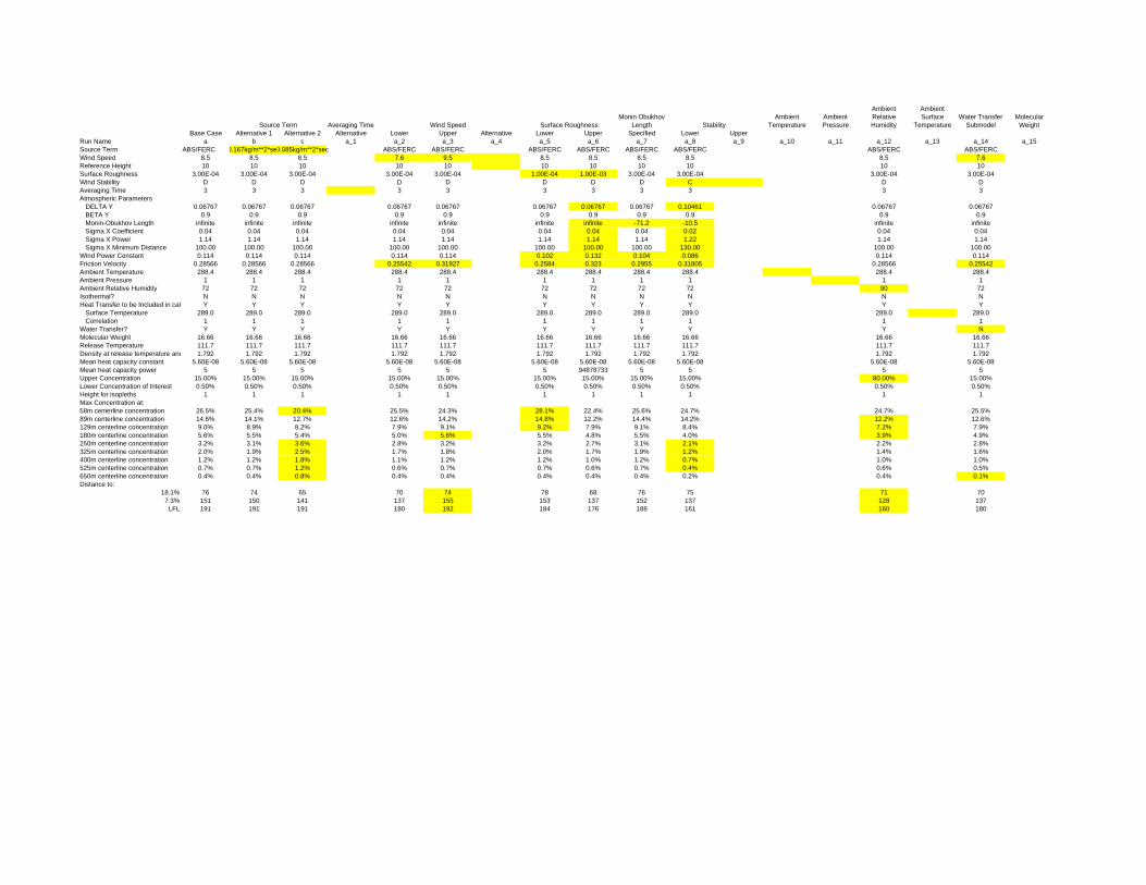
Averaging TimeMonin Obukhov
LengthAmbient
TemperatureAmbient Pressure
Ambient Relative Humidity
Ambient Surface
TemperatureWater Transfer
SubmodelMolecular
WeightBase Case Alternative 1 Alternative 2 Alternative Lower Upper Alternative Lower Upper Specified Lower Upper
Run Name a b c a_1 a_2 a_3 a_4 a_5 a_6 a_7 a_8 a_9 a_10 a_11 a_12 a_13 a_14 a_15Source Term ABS/FERC 0.167kg/m**2*sec0.085kg/m**2*sec ABS/FERC ABS/FERC ABS/FERC ABS/FERC ABS/FERC ABS/FERC ABS/FERC ABS/FERCWind Speed 8.5 8.5 8.5 7.6 9.5 8.5 8.5 8.5 8.5 8.5 7.6Reference Height 10 10 10 10 10 10 10 10 10 10 10Surface Roughness 3.00E-04 3.00E-04 3.00E-04 3.00E-04 3.00E-04 1.00E-04 1.00E-03 3.00E-04 3.00E-04 3.00E-04 3.00E-04Wind Stability D D D D D D D D C D DAveraging Time 3 3 3 3 3 3 3 3 3 3 3Atmospheric Parameters
DELTA Y 0.06767 0.06767 0.06767 0.06767 0.06767 0.06767 0.06767 0.06767 0.10461 0.06767 0.06767BETA Y 0.9 0.9 0.9 0.9 0.9 0.9 0.9 0.9 0.9 0.9 0.9Monin-Obukhov Length infinite infinite infinite infinite infinite infinite infinite -71.2 -10.5 infinite infiniteSigma X Coefficient 0.04 0.04 0.04 0.04 0.04 0.04 0.04 0.04 0.02 0.04 0.04Sigma X Power 1.14 1.14 1.14 1.14 1.14 1.14 1.14 1.14 1.22 1.14 1.14Sigma X Minimum Distance 100.00 100.00 100.00 100.00 100.00 100.00 100.00 100.00 130.00 100.00 100.00
Wind Power Constant 0.114 0.114 0.114 0.114 0.114 0.102 0.132 0.104 0.086 0.114 0.114Friction Velocity 0.28566 0.28566 0.28566 0.25542 0.31927 0.2584 0.323 0.2955 0.31805 0.28566 0.25542Ambient Temperature 288.4 288.4 288.4 288.4 288.4 288.4 288.4 288.4 288.4 288.4 288.4Ambient Pressure 1 1 1 1 1 1 1 1 1 1 1Ambient Relative Humidity 72 72 72 72 72 72 72 72 72 90 72Isothermal? N N N N N N N N N N NHeat Transfer to be Included in cal Y Y Y Y Y Y Y Y Y Y Y
Surface Temperature 289.0 289.0 289.0 289.0 289.0 289.0 289.0 289.0 289.0 289.0 289.0Correlation 1 1 1 1 1 1 1 1 1 1 1
Water Transfer? Y Y Y Y Y Y Y Y Y Y NMolecular Weight 16.66 16.66 16.66 16.66 16.66 16.66 16.66 16.66 16.66 16.66 16.66Release Temperature 111.7 111.7 111.7 111.7 111.7 111.7 111.7 111.7 111.7 111.7 111.7Density at release temperature and 1.792 1.792 1.792 1.792 1.792 1.792 1.792 1.792 1.792 1.792 1.792Mean heat capacity constant 5.60E-08 5.60E-08 5.60E-08 5.60E-08 5.60E-08 5.60E-08 5.60E-08 5.60E-08 5.60E-08 5.60E-08 5.60E-08Mean heat capacity power 5 5 5 5 5 5 94878733 5 5 5 5Upper Concentration 15.00% 15.00% 15.00% 15.00% 15.00% 15.00% 15.00% 15.00% 15.00% 80.00% 15.00%Lower Concentration of Interest 0.50% 0.50% 0.50% 0.50% 0.50% 0.50% 0.50% 0.50% 0.50% 0.50% 0.50%Height for isopleths 1 1 1 1 1 1 1 1 1 1 1Max Concentration at:58m centerline concentration 26.5% 25.4% 20.4% 25.5% 24.3% 28.1% 22.4% 25.6% 24.7% 24.7% 25.5%89m centerline concentration 14.6% 14.1% 12.7% 12.6% 14.2% 14.8% 12.2% 14.4% 14.2% 12.2% 12.6%129m centerline concentration 9.0% 8.9% 8.2% 7.9% 9.1% 9.2% 7.9% 9.1% 8.4% 7.2% 7.9%180m centerline concentration 5.6% 5.5% 5.4% 5.0% 5.6% 5.5% 4.8% 5.5% 4.0% 3.9% 4.9%250m centerline concentration 3.2% 3.1% 3.6% 2.8% 3.2% 3.2% 2.7% 3.1% 2.1% 2.2% 2.8%325m centerline concentration 2.0% 1.9% 2.5% 1.7% 1.8% 2.0% 1.7% 1.9% 1.2% 1.4% 1.6%400m centerline concentration 1.2% 1.2% 1.8% 1.1% 1.2% 1.2% 1.0% 1.2% 0.7% 1.0% 1.0%525m centerline concentration 0.7% 0.7% 1.2% 0.6% 0.7% 0.7% 0.6% 0.7% 0.4% 0.6% 0.5%650m centerline concentration 0.4% 0.4% 0.8% 0.4% 0.4% 0.4% 0.4% 0.4% 0.2% 0.4% 0.1%Distance to:
18.1% 76 74 65 70 74 78 68 76 75 71 707.3% 151 150 141 137 155 153 137 152 137 128 137
LFL 191 191 191 180 192 184 176 188 161 160 180
Source Term Wind Speed Surface Roughness Stability
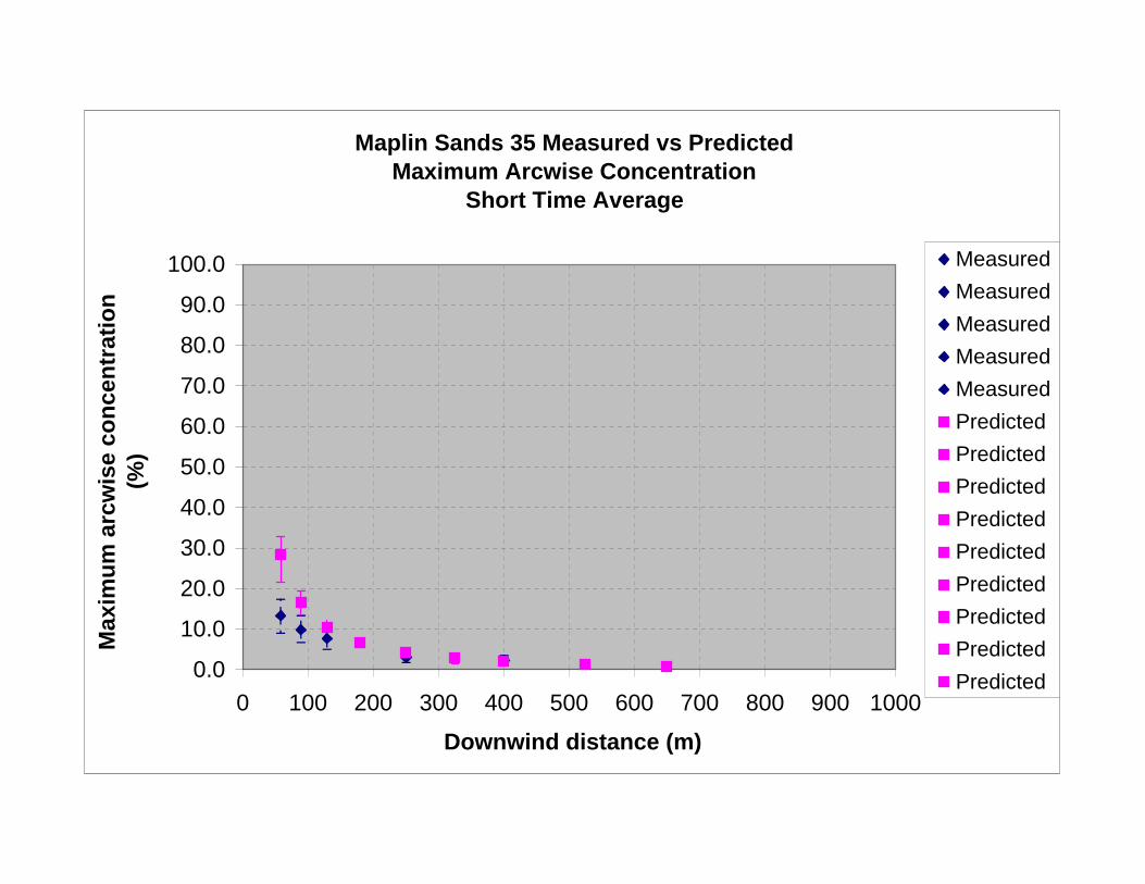
Maplin Sands 35 Measured vs Predicted Maximum Arcwise Concentration
Short Time Average
0.0
10.0
20.0
30.0
40.0
50.0
60.0
70.0
80.0
90.0
100.0
0 100 200 300 400 500 600 700 800 900 1000
Downwind distance (m)
Max
imu
m a
rcw
ise
con
cen
trat
ion
(%
)
Measured
Measured
Measured
Measured
Measured
Predicted
Predicted
Predicted
Predicted
Predicted
Predicted
Predicted
Predicted
Predicted
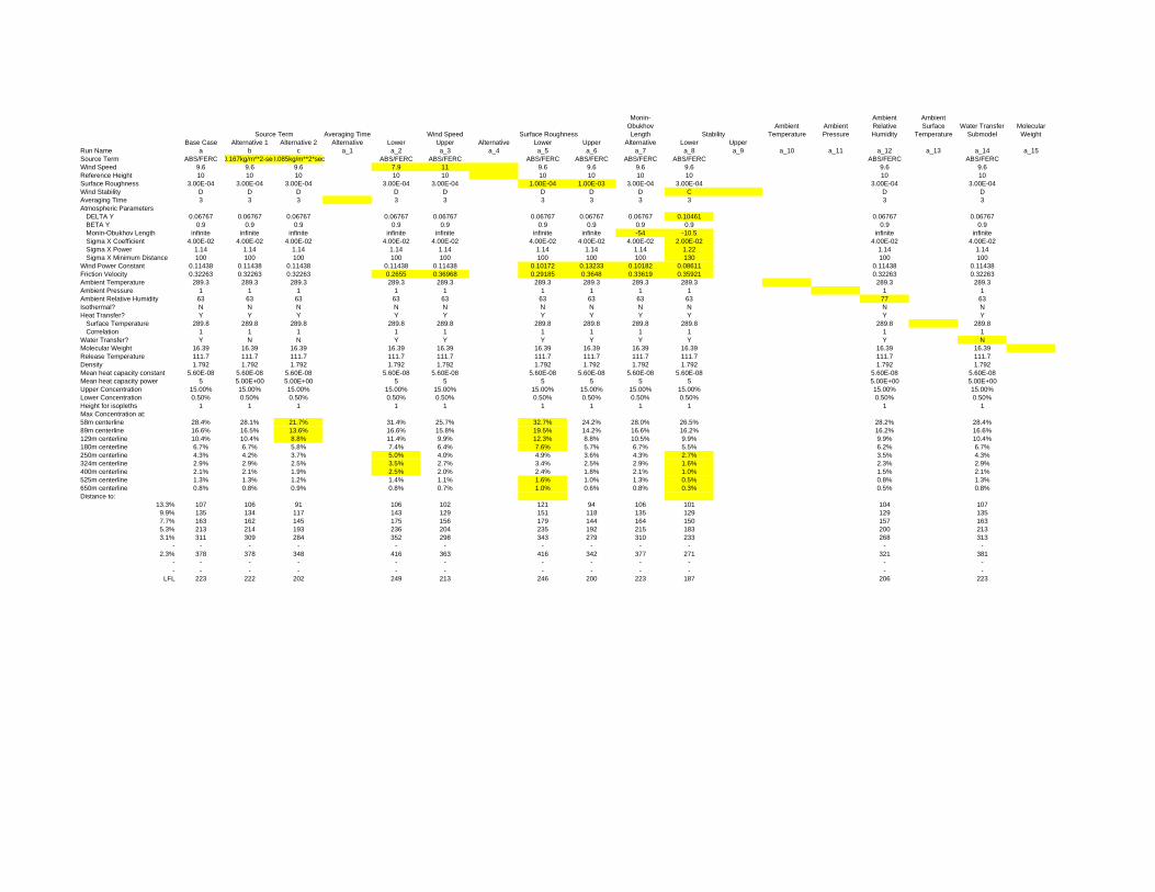
Averaging Time
Monin-Obukhov Length
Ambient Temperature
Ambient Pressure
Ambient Relative Humidity
Ambient Surface
TemperatureWater Transfer
SubmodelMolecular
WeightBase Case Alternative 1 Alternative 2 Alternative Lower Upper Alternative Lower Upper Alternative Lower Upper
Run Name a b c a_1 a_2 a_3 a_4 a_5 a_6 a_7 a_8 a_9 a_10 a_11 a_12 a_13 a_14 a_15Source Term ABS/FERC 0.167kg/m**2-sec0.085kg/m**2*sec ABS/FERC ABS/FERC ABS/FERC ABS/FERC ABS/FERC ABS/FERC ABS/FERC ABS/FERCWind Speed 9.6 9.6 9.6 7.9 11 9.6 9.6 9.6 9.6 9.6 9.6Reference Height 10 10 10 10 10 10 10 10 10 10 10Surface Roughness 3.00E-04 3.00E-04 3.00E-04 3.00E-04 3.00E-04 1.00E-04 1.00E-03 3.00E-04 3.00E-04 3.00E-04 3.00E-04Wind Stability D D D D D D D D C D DAveraging Time 3 3 3 3 3 3 3 3 3 3 3Atmospheric Parameters
DELTA Y 0.06767 0.06767 0.06767 0.06767 0.06767 0.06767 0.06767 0.06767 0.10461 0.06767 0.06767BETA Y 0.9 0.9 0.9 0.9 0.9 0.9 0.9 0.9 0.9 0.9 0.9Monin-Obukhov Length infinite infinite infinite infinite infinite infinite infinite -54 -10.5 infinite infiniteSigma X Coefficient 4.00E-02 4.00E-02 4.00E-02 4.00E-02 4.00E-02 4.00E-02 4.00E-02 4.00E-02 2.00E-02 4.00E-02 4.00E-02Sigma X Power 1.14 1.14 1.14 1.14 1.14 1.14 1.14 1.14 1.22 1.14 1.14Sigma X Minimum Distance 100 100 100 100 100 100 100 100 130 100 100
Wind Power Constant 0.11438 0.11438 0.11438 0.11438 0.11438 0.10172 0.13233 0.10182 0.08611 0.11438 0.11438Friction Velocity 0.32263 0.32263 0.32263 0.2655 0.36968 0.29185 0.3648 0.33619 0.35921 0.32263 0.32263Ambient Temperature 289.3 289.3 289.3 289.3 289.3 289.3 289.3 289.3 289.3 289.3 289.3Ambient Pressure 1 1 1 1 1 1 1 1 1 1 1Ambient Relative Humidity 63 63 63 63 63 63 63 63 63 77 63Isothermal? N N N N N N N N N N NHeat Transfer? Y Y Y Y Y Y Y Y Y Y Y
Surface Temperature 289.8 289.8 289.8 289.8 289.8 289.8 289.8 289.8 289.8 289.8 289.8Correlation 1 1 1 1 1 1 1 1 1 1 1
Water Transfer? Y N N Y Y Y Y Y Y Y NMolecular Weight 16.39 16.39 16.39 16.39 16.39 16.39 16.39 16.39 16.39 16.39 16.39Release Temperature 111.7 111.7 111.7 111.7 111.7 111.7 111.7 111.7 111.7 111.7 111.7Density 1.792 1.792 1.792 1.792 1.792 1.792 1.792 1.792 1.792 1.792 1.792Mean heat capacity constant 5.60E-08 5.60E-08 5.60E-08 5.60E-08 5.60E-08 5.60E-08 5.60E-08 5.60E-08 5.60E-08 5.60E-08 5.60E-08Mean heat capacity power 5 5.00E+00 5.00E+00 5 5 5 5 5 5 5.00E+00 5.00E+00Upper Concentration 15.00% 15.00% 15.00% 15.00% 15.00% 15.00% 15.00% 15.00% 15.00% 15.00% 15.00%Lower Concentration 0.50% 0.50% 0.50% 0.50% 0.50% 0.50% 0.50% 0.50% 0.50% 0.50% 0.50%Height for isopleths 1 1 1 1 1 1 1 1 1 1 1Max Concentration at:58m centerline 28.4% 28.1% 21.7% 31.4% 25.7% 32.7% 24.2% 28.0% 26.5% 28.2% 28.4%89m centerline 16.6% 16.5% 13.6% 16.6% 15.8% 19.5% 14.2% 16.6% 16.2% 16.2% 16.6%129m centerline 10.4% 10.4% 8.8% 11.4% 9.9% 12.3% 8.8% 10.5% 9.9% 9.9% 10.4%180m centerline 6.7% 6.7% 5.8% 7.4% 6.4% 7.6% 5.7% 6.7% 5.5% 6.2% 6.7%250m centerline 4.3% 4.2% 3.7% 5.0% 4.0% 4.9% 3.6% 4.3% 2.7% 3.5% 4.3%324m centerline 2.9% 2.9% 2.5% 3.5% 2.7% 3.4% 2.5% 2.9% 1.6% 2.3% 2.9%400m centerline 2.1% 2.1% 1.9% 2.5% 2.0% 2.4% 1.8% 2.1% 1.0% 1.5% 2.1%525m centerline 1.3% 1.3% 1.2% 1.4% 1.1% 1.6% 1.0% 1.3% 0.5% 0.8% 1.3%650m centerline 0.8% 0.8% 0.9% 0.8% 0.7% 1.0% 0.6% 0.8% 0.3% 0.5% 0.8%Distance to:
13.3% 107 106 91 106 102 121 94 106 101 104 1079.9% 135 134 117 143 129 151 118 135 129 129 1357.7% 163 162 145 175 156 179 144 164 150 157 1635.3% 213 214 193 236 204 235 192 215 183 200 2133.1% 311 309 284 352 298 343 279 310 233 268 313
- - - - - - - - - - - -2.3% 378 378 348 416 363 416 342 377 271 321 381
- - - - - - - - - - - -- - - - - - - - - - - -
LFL 223 222 202 249 213 246 200 223 187 206 223
StabilitySource Term Wind Speed Surface Roughness

Burro 3 Measured vs Predicted Maximum Arcwise Concentration
Short Time Average
0.0
10.0
20.0
30.0
40.0
50.0
60.0
70.0
80.0
90.0
100.0
0 100 200 300 400 500 600 700 800 900 1000
Downwind distance (m)
Max
imu
m a
rcw
ise
con
cen
trat
ion
(%
)
Measured
Measured
Measured
Measured
Predicted
Predicted
Predicted
Predicted

Burro 3 Measured vs Predicted Maximum Arcwise Concentration
Long Time Average
0.0
10.0
20.0
30.0
40.0
50.0
60.0
70.0
80.0
90.0
100.0
0 100 200 300 400 500 600 700 800 900 1000
Downwind distance (m)
Max
imu
m a
rcw
ise
con
cen
trat
ion
(%
)
Measured
Measured
Measured
Predicted
Predicted
Predicted
Predicted

Averaging Time
Monin-Obukhov Length
Ambient Temperature
Ambient Pressure
Ambient Relative Humidity
Ambient Surface
Temperature
Water Transfer
SubmodelMolecular
WeightBase Case Alternative 1 Alternative 2 Alternative Lower Upper Alternative Lower Upper Alternative Lower Upper
Run Name a b c a_1 a_2 a_3 a_4 a_5 a_6 a_7 a_8 a_9 a_10 a_11 a_12 a_13 a_14 a_15Source Term ABS/FERC 0.167kg/m^2*sec0.085kg/m^2*sec ABS/FERC ABS/FERC ABS/FERC ABS/FERC case ABS/FERC ABS/FERCWind Speed 5.4 5.4 5.4 5.4 5.1 5.8 5.58 5.4 5.4 5.4Reference Height 2 2 2 2 2 2 3 2 2 2Surface Roughness 2.00E-04 2.00E-04 2.00E-04 2.00E-04 2.00E-04 2.00E-04 2.00E-04 1.00E-02 2.00E-04 2.00E-04Wind Stability C C C C C C C C D CAveraging Time 1 1 1 100 1 1 1 1 1 1Atmospheric Parameters
DELTA Y 0.10461 0.10461 0.10461 0.14675 0.10461 0.10461 0.10461 0.10461 0.06767 0.10461BETA Y 0.9 0.9 0.9 0.9 0.9 0.9 0.9 0.9 0.9 0.9Monin-Obukhov L -9.26 -9.26 -9.26 -9.26 -9.26 -9.26 -9.26 -30.4 infinite -9.26Sigma X Coefficie 2.00E-02 2.00E-02 2.00E-02 2.00E-02 2.00E-02 2.00E-02 2.00E-02 2.00E-02 4.00E-02 2.00E-02Sigma X Power 1.22 1.22 1.22 1.22 1.22 1.22 1.22 1.22 1.14 1.22Sigma X Minimum 130 130 130 130 130 130 130 130 100 130
Wind Power Consta 0.110 0.110 0.110 0.110 0.110 0.110 0.102 0.227 0.127 0.110Friction Velocity 0.21611 0.21611 0.21611 0.21611 0.2041 0.23212 0.21659 0.36994 0.2052 0.21611Ambient Temperatu 307.75 307.75 307.75 307.75 307.75 307.75 307.75 307.75 307.75 307.75Ambient Pressure 0.936 0.936 0.936 0.936 0.936 0.936 0.936 0.936 0.936 0.936Ambient Relative H 5.2 5.2 5.2 5.2 5.2 5.2 5.2 5.2 5.2 5.2Isothermal? N N N N N N N N N NHeat Transfer to be Y Y Y Y Y Y Y Y Y Y
Surface Tempera 307.75 307.75 307.75 307.75 307.75 307.75 307.75 307.75 307.75 307.75Correlation 1 1 1 1 1 1 1 1 1 1
Water Transfer? N N N N N N N N N NMolecular Weight 17.26 17.26 17.26 17.26 17.26 17.26 17.26 17.26 17.26 16.04Release Temperatu 111.7 111.7 111.7 111.7 111.7 111.7 111.7 111.7 111.7 111.7Density at release t 1.6773 1.6773 1.6773 1.6773 1.6773 1.6773 1.6773 1.6773 1.6773 1.6773Mean heat capacity 5.60E-08 5.60E-08 5.60E-08 5.60E-08 5.60E-08 5.60E-08 5.60E-08 5.60E-08 5.60E-08 5.60E-08Mean heat capacity 5.00E+00 5.00E+00 5.00E+00 5.00E+00 5.00E+00 5.00E+00 5.00E+00 5.00E+00 5.00E+00 5.00E+00Upper Concentratio 80.00% 80.00% 15.00% 80.00% 80.00% 80.00% 80.00% 80.00% 80.00% 80.00%Lower Concentratio 0.50% 1.00% 0.50% 0.50% 0.50% 0.50% 0.50% 1.00% 0.50% 0.50%Height for isopleths 1 1 1 1 1 1 1 1 1 1Max Concentration at:57m centerline 66.7% 66.3% 64.4% 66.7% 68.3% 64.5% 67.0% 41.2% 68.0% 68.5%140m centerline 25.3% 25.2% 25.1% 25.3% 26.0% 24.8% 25.1% 12.2% 26.6% 27.5%400m centerline 5.1% 5.0% 4.9% 4.9% 5.2% 5.0% 5.1% 2.4% 5.3% 5.5%800m centerline 1.2% 1.2% 1.6% 0.8% 1.1% 1.3% 1.2% 0.5% 1.8% 1.7%x=40, y=-40.6, z=1 0.0% 0.0% 0.0% 0.0% 0.0% 0.0% 0.0% 0.0% 0.0% 0.0%x=49, y=-28.7, z=1 0.8% 1.0% 1.1% 1.2% 1.0% 0.5% 0.8% 1.3% 0.4% 0.8%x=55.6, y=-14.9, z= 13.2% 12.8% 11.2% 12.4% 13.8% 12.4% 13.0% 19.8% 14.2% 13.0%x=55.6, y=14.9, z= 14.1% 13.4% 11.4% 13.5% 14.4% 13.5% 13.9% 21.1% 14.2% 13.7%x=49, y=28.7, z=1 1.5% 1.8% 2.0% 2.0% 1.8% 1.1% 1.4% 2.4% 1.0% 1.5%x=37, y=38, z=1 0.0% 0.2% 0.0% 0.1% 0.1% 0.0% 0.0% 0.1% 0.0% 0.0%x=127, y=58, z=1 0.4% 0.4% 0.7% 0.7% 0.4% 0.3% 0.4% 0.2% 0.1% 0.5%x=140, y=0, z=1 13.5% 13.3% 12.1% 13.5% 14.0% 13.1% 13.4% 9.4% 14.0% 14.0%x=395.5, y=-59.8, z 1.0% 1.0% 1.4% 1.1% 1.0% 0.9% 1.0% 0.3% 0.8% 1.4%x=796, y=79.9, z=1 0.5% 0.6% 0.7% 0.5% 0.5% 0.6% 0.5% 0.2% 0.5% 0.8%x=184, y=159, z=1 0.0% 0.0% 0.1% 0.1% 0.0% 0.0% 0.0% 0.0% 0.0% 0.1%Distance to:
28.2% 127 127 128 127 131 126 127 77 134 1379.0% 279 276 275 279 281 274 278 173 285 2940.9% 892 904 990 750 879 895 887 622 1104 10230.5% 1129 1142 1237 944 1114 997 1123 812 1418 1279LFL 405 402 394 395 414 397 404 257 414 424
Source Term Wind Speed Surface Roughness Stability

Burro 7 Measured vs Predicted Maximum Arcwise Concentration
Short Time Average
0.0
10.0
20.0
30.0
40.0
50.0
60.0
70.0
80.0
90.0
100.0
0 100 200 300 400 500 600 700 800 900 1000
Downwind distance (m)
Max
imu
m a
rcw
ise
con
cen
trat
ion
(%
)
MeasuredMeasuredMeasuredPredictedPredictedPredictedPredicted

Burro 7 Measured vs Predicted Maximum Arcwise Concentration
Long Time Average
0.0
10.0
20.0
30.0
40.0
50.0
60.0
70.0
80.0
90.0
100.0
0 100 200 300 400 500 600 700 800 900 1000
Downwind distance (m)
Max
imu
m a
rcw
ise
con
cen
trat
ion
(%
)
MeasuredMeasuredMeasuredPredictedPredictedPredictedPredicted

Averaging TimeMonin-Obukhov
Length Ambient PressureAmbient Relative
Humidity
Water Transfer
Submodel Molecular WeightBase Case Alternative 1 Alternative 2 Alternative Lower Upper Alternative Lower Upper Alternative Lower Upper
Run Name a b c a_1 a_2 a_3 a_4 a_5 a_6 a_7 a_8 a_9 a_11 a_12 a_14 a_15Source Term ABS/FERC 0.167kg/m^2*sec 0.085kg/m^2*sec ABS/FERC ABS/FERC ABS/FERC ABS/FERC ABS/FERC ABS/FERC ABS/FERC ABS/FERCWind Speed 8.4 8.4 8.4 8.4 8.75 8.4 8.4 8.4 8.4 8.4 8.4Reference Height 2 2 2 2 3 2 2 2 2 2 2Surface Roughnes 2.00E-04 2.00E-04 2.00E-04 2.00E-04 2.00E-04 1.00E-02 2.00E-04 2.00E-04 2.00E-04 2.00E-04 2.00E-04Wind Stability D D D D D D D C D D DAveraging Time 1 1 1 140 1 1 1 1 1 1 1Atmospheric Parameters
DELTA Y 0.06767 0.06767 0.06767 0.10166 0.06767 0.06767 0.06767 0.10461 0.06767 0.06767 0.06767BETA Y 0.9 0.9 0.9 0.9 0.9 0.9 0.9 0.9 0.9 0.9 0.9Monin-Obukhov infinite infinite infinite infinite infinite infinite -114 -9.26 power infinite infiniteSigma X Coeffici 4.00E-02 4.00E-02 4.00E-02 4.00E-02 4.00E-02 4.00E-02 4.00E-02 2.00E-02 4.00E-02 4.00E-02 4.00E-02Sigma X Power 1.14 1.14 1.14 1.14 1.14 1.14 1.14 1.22 1.14 1.14 1.14Sigma X Minimu 100 100 100 100 100 100 100 130 100 100 100
Wind Power Const 0.127 0.127 0.127 0.127 0.122 0.110 0.125 0.110 0.127 0.127 0.127Friction Velocity 0.3192 0.3192 0.3192 0.3192 0.31848 0.55437 0.32134 0.33617 0.3192 0.3192 0.3192Ambient Temperat 306.96 306.96 306.96 306.96 306.96 306.96 306.96 306.96 306.96 306.96 306.96Ambient Pressure 0.928 0.928 0.928 0.928 0.928 0.928 0.928 0.928 1 0.928 0.928Ambient Relative H 7.4 7.4 7.4 7.4 7.4 7.4 7.4 7.4 7.4 5 7.4Isothermal? N N N N N N N N N N NHeat Transfer to be Y Y Y Y Y Y Y Y Y Y Y
Surface Tempera 306.96 306.96 306.96 306.96 306.96 306.96 306.96 306.96 306.96 306.96 306.96Correlation 1 1 1 1 1 1 1 1 1 1 1
Water Transfer? N N N N N N N N N N NMolecular Weight 18.22 18.22 18.22 18.22 18.22 18.22 18.22 18.22 18.22 18.22 16.04Release Temperat 111.7 111.7 111.7 111.7 111.7 111.7 111.7 111.7 111.7 111.7 111.7Density at release 1.663 1.663 1.663 1.663 1.663 1.663 1.663 1.663 1.792 1.663 1.663Mean heat capacit 5.60E-08 5.60E-08 5.60E-08 5.60E-08 5.60E-08 5.60E-08 5.60E-08 5.60E-08 5.60E-08 5.60E-08 5.60E-08Mean heat capacit 5.00E+00 5.00E+00 5.00E+00 5.00E+00 5.00E+00 5.00E+00 5.00E+00 5.00E+00 5.00E+00 5.00E+00 5.00E+00Upper Concentrati 8.00E-01 8.00E-01 8.00E-01 8.00E-01 8.00E-01 8.00E-01 8.00E-01 8.00E-01 8.00E-01 8.00E-01 8.00E-01Lower Concentrati 5.00E-03 1.00E-02 5.00E-03 5.00E-03 5.00E-03 5.00E-03 5.00E-03 5.00E-03 5.00E-03 5.00E-03 5.00E-03Height for isopleths 1 1 1 1 1 1 1 1 1 1 1Max Concentration at:57m centerline 61.2% 60.7% 49.4% 61.2% 61.4% 33.9% 60.9% 60.0% 60.0% 58.9% 64.1%140m centerline 22.7% 22.4% 20.2% 22.7% 23.2% 11.0% 22.5% 21.4% 21.5% 22.7% 26.7%400m centerline 4.8% 4.8% 4.4% 4.8% 4.8% 2.4% 4.8% 4.6% 4.6% 4.8% 5.3%800m centerline 1.7% 1.7% 1.5% 1.1% 1.7% 0.9% 1.7% 0.9% 1.6% 1.7% 1.8%x=57, y=0, z=1 10.2% 9.6% 13.2% 9.5% 10.0% 12.0% 10.1% 9.0% 9.2% 10.2% 9.9%
x=55.6, y=14.9, z=1 15.5% 15.3% 15.0% 15.5% 15.5% 19.6% 15.8% 16.1% 15.2% 15.4% 14.9%x=49, y=-28.7, z=1 14.1% 13.7% 15.0% 12.9% 13.8% 17.7% 13.9% 12.5% 13.1% 14.0% 13.5%
x=37, y=38, z=1 0.2% 0.1% 0.7% 0.5% 0.2% 0.2% 0.2% 0.4% 0.1% 0.2% 0.2%x=140, y=0, z=1 0.6% 0.6% 1.2% 1.1% 0.6% 0.4% 0.6% 0.9% 0.5% 0.7% 1.1%x=137, y=30, z=1 12.8% 12.7% 11.2% 12.7% 13.2% 8.6% 12.9% 12.3% 12.4% 12.8% 13.6%x=127, y=58, z=1 10.6% 10.5% 10.6% 9.7% 10.8% 7.3% 10.5% 9.1% 9.7% 10.8% 12.5%x=112, y=84, z=1 0.1% 0.1% 0.2% 0.2% 0.1% 0.0% 0.1% 0.2% 0.0% 0.1% 0.1%x=382, y=118, z=1 4.0% 4.0% 3.6% 4.0% 4.1% 2.2% 4.0% 3.9% 3.8% 4.0% 4.3%x=360, y=174, z=1 0.3% 0.3% 0.6% 0.5% 0.3% 0.2% 0.3% 0.4% 0.2% 0.3% 0.8%
Distance to:17.9% 167 166 155 167 167 94 167 160 161 167 1847.1% 310 307 292 310 310 192 310 306 300 309 3343.9% 468 462 435 461 468 287 468 440 452 465 491
LFL 388 387 368 388 390 242 388 381 374 386 414
Source Term Wind Speed Surface Roughness Stability
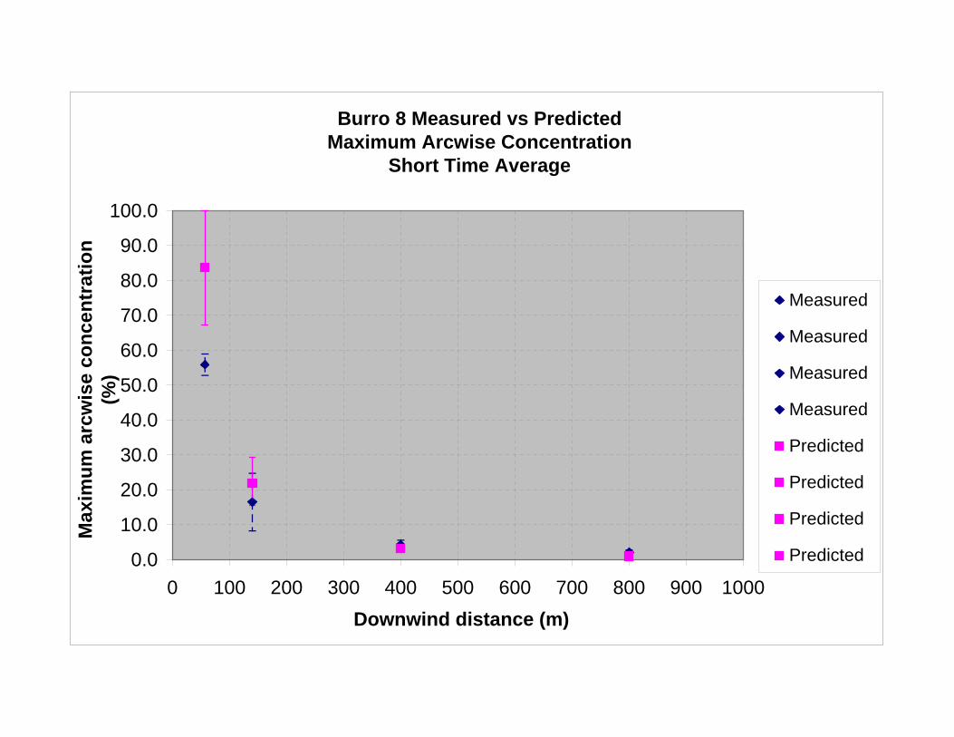
Burro 8 Measured vs Predicted Maximum Arcwise Concentration
Short Time Average
0.0
10.0
20.0
30.0
40.0
50.0
60.0
70.0
80.0
90.0
100.0
0 100 200 300 400 500 600 700 800 900 1000
Downwind distance (m)
Max
imu
m a
rcw
ise
con
cen
trat
ion
(%
)
Measured
Measured
Measured
Measured
Predicted
Predicted
Predicted
Predicted

Burro 8 Measured vs Predicted Maximum Arcwise Concentration
Long Time Average
0.0
10.0
20.0
30.0
40.0
50.0
60.0
70.0
80.0
90.0
100.0
0 100 200 300 400 500 600 700 800 900
Downwind distance (m)
Max
imu
m a
rcw
ise
con
cen
trat
ion
(%
)
Measured
Measured
Measured
Measured
Predicted
Predicted
Predicted
Predicted

Averaging Time
Monin-Obukhov Length
Ambient Temperature
Ambient Pressure
Ambient Relative Humidity
Ambient Surface
TemperatureWater Transfer
SubmodelMolecular
WeightBase Case Alternative 1 Alternative 2 Alternative Lower Upper Alternative Lower Upper Alternative Lower Upper
Run Name a b c a_1 a_2 a_3 a_4 a_5 a_6 a_7 a_8 a_9 a_10 a_11 a_12 a_13 a_14 a_15Source Term ABS/FERC 0.167kg/m^2*sec0.085kg/m^2*se ABS/FERC ABS/FERC ABS/FERC ABS/FERC ABS/FERC ABS/FERC ABS/FERC ABS/FERCWind Speed 1.8 1.8 1.8 1.8 1.5 2 1.94 1.8 1.8 1.8 1.8Reference Height 2 2 2 2 2 2 3 2 2 2 2Surface Roughness 2.00E-04 2.00E-04 2.00E-04 2.00E-04 2.00E-04 2.00E-04 2.00E-04 1.00E-02 1.33E-03 2.00E-04 2.00E-04Wind Stability E E E E E E E E E F EAveraging Time 1 1 1 100 1 1 1 1 1 1 1Atmospheric Parameters
DELTA Y 0.04617 0.04617 0.04617 0.07128 0.04617 0.04617 0.04617 0.04617 0.04617 0.02544 0.04617BETA Y 0.9 0.9 0.9 0.9 0.9 0.9 0.9 0.9 0.9 0.9 0.9Monin-Obukhov Length 9.26 9.26 9.26 9.26 9.26 9.26 9.26 30.4 16.5 6.06 9.26Sigma X Coefficient 1.70E-01 1.70E-01 1.70E-01 1.70E-01 1.70E-01 1.70E-01 1.70E-01 1.70E-01 1.70E-01 1.70E-01 1.70E-01Sigma X Power 0.97 0.97 0.97 0.97 0.97 0.97 0.97 0.97 0.97 0.97 0.97Sigma X Minimum Distance 50 50 50 50 50 50 50 50 50 50 50
Wind Power Constant 0.168 0.168 0.168 0.168 0.168 0.168 0.178 0.262 0.195 0.188 0.168Friction Velocity 0.06161 0.06161 0.06161 0.06161 0.05134 0.06846 0.06096 0.11226 0.07988 0.05853 0.06161Ambient Temperature 306.02 306.02 306.02 306.02 306.02 306.02 306.02 306.02 306.02 306.02 306.02Ambient Pressure 0.929 0.929 0.929 0.929 0.929 0.929 0.929 0.929 0.929 0.929 0.929Ambient Relative Humidity 4.5 4.5 4.5 4.5 4.5 4.5 4.5 4.5 4.5 4.5 4.5Isothermal? N N N N N N N N N N NHeat Transfer? Y Y Y Y Y Y Y Y Y Y Y
Surface Temperature 306.02 306.02 306.02 306.02 306.02 306.02 306.02 306.02 306.02 306.02 306.02Correlation 1 1 1 1 1 1 1 1 1 1 1
Water Transfer? N N N N N N N N N N NMolecular Weight 18.12 18.12 18.12 18.12 18.12 18.12 18.12 18.12 18.12 18.12 16.04Release Temperature 111.7 111.7 111.7 111.7 111.7 111.7 111.7 111.7 111.7 111.7 111.7Density 1.6648 1.6648 1.6648 1.6648 1.6648 1.6648 1.6648 1.6648 1.6648 1.6648 1.6648Mean heat capacity constant 5.60E-08 5.60E-08 5.60E-08 5.60E-08 5.60E-08 5.60E-08 5.60E-08 5.60E-08 5.60E-08 5.60E-08 5.60E-08Mean heat capacity power 5 5.00E+00 5.00E+00 5.00E+00 5.00E+00 5.00E+00 5 5.00E+00 5.00E+00 5.00E+00 5.00E+00Upper Concentration 0.8 8.00E-01 8.00E-01 8.00E-01 8.00E-01 8.00E-01 0.8 8.00E-01 8.00E-01 8.00E-01 8.00E-01Lower Concentration 0.005 5.00E-03 5.00E-03 5.00E-03 5.00E-03 5.00E-03 5.00E-03 5.00E-03 5.00E-03 5.00E-03 5.00E-03Height for isopleths 1 1 1 1 1 1 1 1 1 1 1Max Concentration at:57m centerline 83.8% 100.0% 100.0% 83.8% 88.3% 89.8% 83.9% 67.2% 85.5% 80.2% 68.9%140m centerline 22.0% 22.5% 21.0% 22.0% 16.3% 25.1% 21.9% 15.7% 23.1% 21.8% 29.4%400m centerline 3.1% 2.9% 3.3% 3.1% 2.1% 3.6% 3.1% 3.5% 3.5% 2.9% 5.3%800m centerline 1.0% 1.0% 1.1% 1.0% 0.7% 1.2% 1.0% 1.3% 1.1% 1.0% 1.5%x=40, y=-40.6, z=1 32.2% 22.7% 30.6% 32.2% 16.3% 24.3% 11.9% 34.4% 25.0% 29.4% 30.9%x=49, y=-28.7, z=1 30.1% 24.8% 30.2% 30.1% 15.2% 24.7% 14.4% 43.6% 26.4% 28.3% 30.5%x=57, y=0, z=1 29.5% 25.3% 30.2% 29.5% 14.9% 25.3% 14.3% 42.4% 26.9% 27.9% 30.1%x=55.6, y=14.9, z=1 30.3% 24.7% 30.2% 30.3% 15.3% 24.6% 14.3% 43.9% 26.2% 28.4% 30.7%x=49, y=-28.7, z=1 33.0% 21.3% 31.0% 33.0% 16.8% 24.2% 5.4% 10.6% 20.3% 30.6% 30.9%x=37, y=38, z=1 34.5% 13.5% 35.3% 34.5% 18.5% 1.0% 0.0% 0.0% 0.2% 35.1% 32.7%x=112, y=-84, z=1 12.4% 16.2% 10.5% 11.5% 13.0% 12.0% 12.3% 0.4% 13.6% 13.9% 20.9%x=127, y=-58, z=1 17.2% 16.2% 17.6% 17.2% 13.1% 18.1% 17.1% 12.6% 17.9% 15.2% 20.0%x=137, y=-30, z=1 16.5% 15.1% 16.9% 16.5% 12.3% 17.1% 16.4% 14.0% 17.4% 14.8% 19.5%x=140, y=0, z=1 16.8% 15.6% 17.2% 16.8% 12.6% 17.5% 16.7% 14.3% 17.5% 15.0% 19.7%x=137, y=30, z=1 17.7% 17.2% 16.7% 17.3% 13.8% 19.1% 17.6% 3.2% 18.9% 15.5% 20.5%x=127, y=58, z=1 0.9% 3.5% 0.8% 1.7% 2.2% 0.7% 1.0% 0.0% 0.7% 0.4% 6.9%x=112, y=84, z=1 0.0% 0.0% 0.0% 0.0% 0.0% 0.0% 0.0% 0.0% 0.0% 0.0% 0.0%x=360, y=174, z=1 0.1% 0.1% 0.0% 0.1% 0.0% 0.1% 0.1% 0.0% 0.2% 0.0% 0.9%x=382, y=118, z=1 2.5% 2.4% 2.6% 2.3% 1.8% 3.0% 2.5% 0.9% 3.2% 2.5% 4.9%x=395.5, y=-59.8, z=1 3.0% 2.8% 3.2% 3.0% 2.0% 3.5% 3.0% 3.4% 3.4% 2.8% 4.9%x=400, y=0, z=1 1.3% 1.6% 1.3% 1.4% 1.1% 1.7% 1.3% 0.3% 2.2% 1.5% 4.0%x=395.5, y=59.8, z=1 0.0% 0.0% 0.0% 0.0% 0.0% 0.0% 0.0% 0.0% 0.0% 0.0% 0.3%x=784, y=-159, z=1 1.0% 1.0% 1.0% 1.0% 0.7% 1.2% 1.0% 1.0% 1.1% 1.0% 1.5%x=796, y=-79.9, z=1 0.7% 0.7% 0.6% 0.6% 0.5% 0.8% 0.7% 0.3% 0.8% 0.7% 1.3%x=800, y=0, z=1 0.0% 0.0% 0.0% 0.0% 0.0% 0.0% 0.0% 0.0% 0.0% 0.0% 0.1%Distance to:
55.9% 83 89 84 83 81 83 84 65 77 82 9016.5% 156 160 160 164 138 182 164 135 183 156 2104.3% 324 313 338 324 255 370 322 342 368 304 4412.1% 501 503 535 501 397 558 503 566 540 498 667
LFL 289 291 308 289 221 329 290 302 328 284 415
Source Term Wind Speed Surface Roughness Stability

Burro 9 Measured vs Predicted Maximum Arcwise Concentration
Short Time Average
0.0
10.0
20.0
30.0
40.0
50.0
60.0
70.0
80.0
90.0
100.0
0 100 200 300 400 500 600 700 800 900 1000
Downwind distance (m)
Max
imu
m a
rcw
ise
con
cen
trat
ion
(%
)
Measured
Measured
Measured
Predicted
Predicted
Predicted
Predicted

Burro 9 Measured vs Predicted Maximum Arcwise Concentration
Long Time Average
0.0
10.0
20.0
30.0
40.0
50.0
60.0
70.0
80.0
90.0
100.0
0 100 200 300 400 500 600 700 800 900 1000
Downwind distance (m)
Max
imu
m a
rcw
ise
con
cen
trat
ion
(%
)
Measured
Measured
Measured
Predicted
Predicted
Predicted
Predicted

Averaging Time
Monin-Obukhov Length
Ambient Temperature
Ambient Pressure
Ambient Relative Humidity
Ambient Surface
TemperatureWater Transfer
SubmodelMolecular
WeightBase Case Alternative 1 Alternative 2 Alternative Lower Upper Alternative Lower Upper Alternative Lower Upper
Run Name a b c a_1 a_2 a_3 a_4 a_5 a_6 a_7 a_8 a_9 a_10 a_11 a_12 a_13 a_14 a_15Source Term ABS/FERC 0.167kg/m^2*sec0.085kg/m^2*sec ABS/FERC ABS/FERC ABS/FERC ABS/FERC ABS/FERC ABS/FERC ABS/FERCWind Speed 5.7 5.7 5.7 5.7 5.94 5.7 5.7 5.7 5.7 5.7Reference Height 2 2 2 2 3 2 2 2 2 2Surface Roughness 2.00E-04 2.00E-04 2.00E-04 2.00E-04 2.00E-04 1.00E-02 2.00E-04 2.00E-04 2.00E-04 2.00E-04Wind Stability D D D D D D D C D DAveraging Time 1 1 1 100 1 1 1 1 1 1Atmospheric Parameters
DELTA Y 0.06767 0.06767 0.06767 0.09504 0.06767 0.06767 0.06767 0.10461 0.06767 0.06767BETA Y 0.9 0.9 0.9 0.9 0.9 0.9 0.9 0.9 0.9 0.9Monin-Obukhov Length infinite infinite infinite infinite infinite infinite -141 -9.26 infinite infiniteSigma X Coefficient 4.00E-02 4.00E-02 4.00E-02 4.00E-02 4.00E-02 4.00E-02 4.00E-02 2.00E-02 4.00E-02 4.00E-02Sigma X Power 1.14E+00 1.14E+00 1.14E+00 1.14E+00 1.14E+00 1.14E+00 1.14E+00 1.22E+00 1.14E+00 1.14E+00Sigma X Minimum Distance 1.00E+02 1.00E+02 1.00E+02 1.00E+02 1.00E+02 1.00E+02 1.00E+02 1.30E+02 1.00E+02 1.00E+02
Wind Power Constant 0.127 0.127 0.127 0.127 0.122 0.240 0.125 0.110 0.127 0.127Friction Velocity 0.2166 0.2166 0.2166 0.2166 0.21621 0.37618 0.21779 0.22811 0.2166 0.2166Ambient Temperature 308.52 308.52 308.52 308.52 308.52 308.52 308.52 308.52 308.52 308.52Ambient Pressure 0.928 0.928 0.928 0.928 0.928 0.928 0.928 0.928 0.928 0.928Ambient Relative Humidity 14.4 14.4 14.4 14.4 14.4 14.4 14.4 14.4 6.5 14.4Isothermal? N N N N N N N N N NHeat Transfer? Y Y Y Y Y Y Y Y Y Y
Surface Temperature 308.52 308.52 308.52 308.52 308.52 308.52 308.52 308.52 308.52 308.52Correlation 1 1 1 1 1 1 1 1 1 1
Water Transfer? N N N N N N N N N NMolecular Weight 18.82 18.82 18.82 18.82 18.82 18.82 18.82 18.82 18.82 16.04Release Temperature 111.7 111.7 111.7 111.7 111.7 111.7 111.7 111.7 111.7 111.7Density 1.663 1.663 1.663 1.663 1.663 1.663 1.663 1.663 1.663 1.663Mean heat capacity constant 5.60E-08 5.60E-08 5.60E-08 5.60E-08 5.60E-08 5.60E-08 5.60E-08 5.60E-08 5.60E-08 5.60E-08Mean heat capacity power 5 5 5 5 5 5 5 5 5 5Upper Concentration 80.0% 80.0% 80.0% 80.0% 80.0% 80.0% 80.0% 80.0% 80.0% 80.0%Lower Concentration 0.5% 0.5% 0.5% 0.5% 0.5% 0.5% 0.5% 0.5% 0.5% 0.5%Height for isopleths 1 1 1 1 1 1 1 1 1 1Max Concentration at:57m centerline 76.4% 76.1% 73.6% 76.4% 76.5% 45.7% 76.5% 74.9% 76.9% 79.1%140m centerline 30.6% 29.5% 29.7% 30.6% 31.2% 15.9% 30.8% 30.4% 32.5% 37.5%400m centerline 6.9% 6.6% 6.3% 6.6% 6.9% 3.4% 6.9% 6.7% 6.6% 8.3%800m centerline 2.1% 2.2% 2.2% 1.6% 2.1% 0.9% 2.1% 1.4% 2.0% 2.7%x=127, y=-58, z=1 4.4% 4.53% 6.35% 5.03% 4.63% 1.86% 4.48% 5.23% 5.77% 7.77%x=137, y=-30, z=1 18.2% 17.11% 15.88% 18.23% 18.51% 12.74% 18.21% 18.02% 17.72% 19.29%x=140, y=0, z=1 18.3% 17.18% 15.93% 18.27% 18.50% 12.80% 18.19% 18.03% 17.71% 19.27%x=127, y=58, z=1 0.0% 0.00% 0.01% 0.01% 0.00% 0.00% 0.00% 0.02% 0.00% 0.01%x=382, y=-118, z=1 0.9% 0.92% 1.43% 1.10% 0.86% 0.08% 0.87% 1.14% 0.90% 2.48%x=395.5, y=-59.8, z=1 5.9% 5.60% 5.25% 5.91% 5.94% 3.04% 5.93% 5.77% 5.70% 6.74%x=400, y=0, z=1 3.0% 3.06% 3.66% 2.98% 3.02% 0.61% 3.03% 2.90% 2.99% 5.43%x=784, y=-159, z=1 0.6% 0.73% 1.04% 0.73% 0.63% 0.21% 0.64% 0.69% 0.60% 1.72%x=796, y=-79.9, z=1 1.8% 1.92% 1.99% 1.46% 1.82% 0.79% 1.83% 1.27% 1.70% 2.43%x=800, y=0, z=1 0.1% 0.15% 0.31% 0.24% 0.12% 0.03% 0.12% 0.26% 0.11% 0.69%Distance to:
- - - - - - - - - - 010.6% 298 291 285 298 300 185 299 296 292 3414.0% 552 556 539 546 553 359 553 528 532 6201.4% 960 993 1022 841 959 658 959 800 929 1160
LFL 492 482 465 491 492 307 493 481 462 537
Source Term Wind Speed Surface Roughness Stability
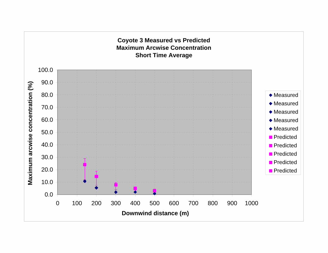
Coyote 3 Measured vs Predicted Maximum Arcwise Concentration
Short Time Average
0.0
10.0
20.0
30.0
40.0
50.0
60.0
70.0
80.0
90.0
100.0
0 100 200 300 400 500 600 700 800 900 1000
Downwind distance (m)
Max
imu
m a
rcw
ise
con
cen
trat
ion
(%
)
Measured
Measured
Measured
Measured
Measured
Predicted
Predicted
Predicted
Predicted
Predicted

Coyote 3 Measured vs Predicted Maximum Arcwise Concentration
Long Time Average
0.0
10.0
20.0
30.0
40.0
50.0
60.0
70.0
80.0
90.0
100.0
0 100 200 300 400 500 600 700 800 900 1000
Downwind distance (m)
Max
imu
m a
rcw
ise
con
cen
trat
ion
(%
)
Measured
Measured
Measured
Measured
Predicted
Predicted
Predicted
Predicted
Measured
Predicted

Averaging Time
Monin-Obukhov Length
Ambient Temperature
Ambient Pressure
Ambient Relative Humidity
Ambient Surface
TemperatureWater Transfer
SubmodelMolecular
WeightBase Case Alternative 1 Alternative 2 Alternative Lower Upper Alternative Lower Upper Alternative Lower Upper
Run Name a b c a_1 a_2 a_3 a_4 a_5 a_6 a_7 a_8 a_9 a_10 a_11 a_12 a_13 a_14 a_15Source Term ABS/FERC 0.167kg/m^2*se0.085kg/m^2*secABS/FERC ABS/FERC ABS/FERC ABS/FERC ABS/FERC ABS/FERC ABS/FERCWind Speed 6 6 6 6 6.77 6 6 6 6 6Reference Height 2 2 2 2 3 2 2 2 2 2Surface Roughness 2.00E-04 2.00E-04 2.00E-04 2.00E-04 2.00E-04 1.00E-02 2.00E-04 2.00E-04 2.00E-04 2.00E-04Wind Stability C C C C C C C D C CAveraging Time 1 1 1 50 1 1 1 1 1 1Atmospheric Parameters
DELTA Y 0.10461 0.10461 0.10461 0.12776 0.10461 0.10461 0.10461 0.06767 0.10461 0.10461BETA Y 0.9 0.9 0.9 0.9 0.9 0.9 0.9 0.9 0.9 0.9Monin-Obukhov Length -9.26 -9.26 -9.26 -9.26 -9.26 -30.4 -6.32 infinite -9.26 -9.26Sigma X Coefficient 2.00E-02 2.00E-02 2.00E-02 2.00E-02 2.00E-02 2.00E-02 2.00E-02 4.00E-02 2.00E-02 2.00E-02Sigma X Power 1.22E+00 1.22E+00 1.22E+00 1.22E+00 1.22E+00 1.22E+00 1.22E+00 1.14E+00 1.22E+00 1.22E+00Sigma X Minimum Distance 1.30E+02 1.30E+02 1.30E+02 1.30E+02 1.30E+02 1.30E+02 1.30E+02 1.00E+02 1.30E+02 1.30E+02
Wind Power Constant 0.110 0.110 0.110 0.110 0.102 0.227 0.106 0.127 0.110 0.110Friction Velocity 0.24012 0.24012 0.24012 0.24012 0.26278 0.41104 0.24362 0.228 0.24012 0.24012Ambient Temperature 311.45 311.45 311.45 311.45 311.45 311.45 311.45 311.45 311.45 311.45Ambient Pressure 0.924 0.924 0.924 0.924 0.924 0.924 0.924 0.924 0.924 0.924Ambient Relative Humidity 11.3 11.3 11.3 11.3 11.3 11.3 11.3 11.3 3.5 11.3Isothermal? N N N N N N N N N NHeat Transfer? Y Y Y Y Y Y Y Y Y Y
Surface Temperature 311.45 311.45 311.45 311.45 311.45 311.45 311.45 311.45 311.45 311.45Correlation 1 1 1 1 1 1 1 1 1 1
Water Transfer? N N N N N N N N N NMolecular Weight 19.51 19.51 19.51 19.51 19.51 19.51 19.51 19.51 19.51 16.04Release Temperature 111.7 111.7 111.7 111.7 111.7 111.7 111.7 111.7 111.7 111.7Density 1.6558 1.6558 1.6558 1.6558 1.6558 1.6558 1.6558 1.6558 1.6558 1.6558Mean heat capacity constant 5.60E-08 5.60E-08 5.60E-08 5.60E-08 5.60E-08 5.60E-08 5.60E-08 5.60E-08 5.60E-08 5.60E-08Mean heat capacity power 5 5.00E+00 5.00E+00 5.00E+00 5.00E+00 5.00E+00 5.00E+00 5.00E+00 5 5.00E+00Upper Concentration 80.0% 8.00E-01 8.00E-01 8.00E-01 8.00E-01 8.00E-01 8.00E-01 8.00E-01 80.0% 8.00E-01Lower Concentration 0.5% 5.00E-03 5.00E-03 5.00E-03 5.00E-03 5.00E-03 5.00E-03 5.00E-03 0.5% 5.00E-03Height for isopleths 1 1 1 1 1 1 1 1 1 1Max Concentration at:140m centerline 23.9% 22.4% 21.4% 23.9% 23.6% 11.9% 23.2% 24.2% 24.0% 29.0%200m centerline 14.6% 13.7% 13.3% 14.6% 14.6% 7.4% 14.6% 15.0% 14.6% 18.6%300m centerline 7.9% 7.6% 7.3% 7.8% 7.8% 4.0% 7.7% 8.1% 7.6% 9.7%400m centerline 4.9% 4.8% 4.7% 4.3% 4.9% 2.2% 5.0% 5.1% 4.6% 6.2%500m centerline 3.0% 2.9% 2.9% 2.4% 3.2% 1.3% 2.9% 3.6% 2.8% 4.3%x=140, y=0, z=1 0.5% 0.4% 0.5% 0.7% 0.4% 0.3% 0.5% 0.2% 0.6% 1.0%x=112, y=84, z=1 4.6% 4.0% 4.4% 4.8% 4.1% 2.8% 4.5% 4.2% 5.2% 6.9%x=127, y=58, z=1 14.2% 13.2% 12.5% 14.2% 13.7% 9.4% 13.8% 14.3% 13.4% 15.0%x=137, y=30, z=1 11.0% 10.0% 10.0% 10.6% 10.3% 7.0% 10.8% 12.3% 11.2% 13.4%x=186.5, y=72, z=1 10.3% 9.6% 9.3% 10.3% 10.1% 6.3% 10.3% 10.5% 10.1% 11.8%x=196.6, y=36.9, z=1 4.0% 3.5% 3.7% 4.0% 3.7% 2.0% 3.9% 3.9% 4.3% 6.6%x=200, y=0, z=1 0.1% 0.0% 0.1% 0.1% 0.0% 0.0% 0.1% 0.0% 0.1% 0.2%x=296, y=48.3, z=1 0.5% 0.5% 0.6% 0.7% 0.5% 0.2% 0.5% 0.3% 0.6% 1.5%x=395.5, y=59.8, z=1 0.1% 0.1% 0.1% 0.1% 0.1% 0.0% 0.1% 0.0% 0.1% 0.4%x=382, y=118, z=1 2.6% 2.5% 2.5% 2.5% 2.6% 1.1% 2.6% 2.8% 2.4% 4.3%x=330, y=226, z=1 0.1% 0.1% 0.1% 0.2% 0.1% 0.0% 0.1% 0.1% 0.1% 0.6%x=495, y=71.2, z=1 0.0% 0.0% 0.0% 0.0% 0.0% 0.0% 0.0% 0.0% 0.0% 0.1%Distance to:
10.7% 257 238 232 241 241 151 246 246 239 2855.4% 379 373 366 367 380 243 374 386 369 4351.9% 593 589 589 542 608 424 584 697 580 8072.0% 582 577 578 534 599 416 575 683 567 7880.8% 832 824 833 764 850 634 820 998 772 1076LFL 392 392 385 378 396 254 399 405 383 453
Source Term Wind Speed Surface Roughness Stability

Coyote 5 Measured vs Predicted Maximum Arcwise Concentration
Short Time Average
0.0
10.0
20.0
30.0
40.0
50.0
60.0
70.0
80.0
90.0
100.0
0 100 200 300 400 500 600 700 800 900 1000
Downwind distance (m)
Max
imu
m a
rcw
ise
con
cen
trat
ion
(%
)
Measured
Measured
Measured
Measured
Measured
Predicted
Predicted
Predicted
Predicted
Predicted

Coyote 5 Measured vs Predicted Maximum Arcwise Concentration
Long Time Average
0.0
10.0
20.0
30.0
40.0
50.0
60.0
70.0
80.0
90.0
100.0
0 100 200 300 400 500 600 700 800 900 1000
Downwind distance (m)
Max
imu
m a
rcw
ise
con
cen
trat
ion
(%
)
Measured
Measured
Measured
Measured
Predicted
Predicted
Predicted
Predicted
Measured
Predicted

Averaging Time
Monin-Obukhov Length
Ambient Temperature
Ambient Pressure
Ambient Relative Humidity
Ambient Surface
TemperatureWater Transfer
SubmodelMolecular
WeightBase Case Alternative 1 Alternative 2 Alternative Lower Upper Alternative Lower Upper Alternative Lower Upper
Run Name a b c a_1 a_2 a_3 a_4 a_5 a_6 a_7 a_8 a_9 a_10 a_11 a_12 a_13 a_14 a_15Source Term ABS/FERC 0.167kg/m^2*se 0.085kg/m^2*se ABS/FERC ABS/FERC ABS/FERC ABS/FERC ABS/FERC ABS/FERC ABS/FERCWind Speed 9.7 9.7 9.7 9.7 10.47 9.7 9.7 9.7 9.7 9.7Reference Height 2 2 2 2 3 2 2 2 2 2Surface Roughness 2.00E-04 2.00E-04 2.00E-04 2.00E-04 2.00E-04 1.00E-02 2.00E-04 2.00E-04 2.00E-04 2.00E-04Wind Stability C C C C C C C D C CAveraging Time 1 1 1 90 1 1 1 1 1 1Atmospheric Parameters
DELTA Y 0.10461 0.10461 0.10461 0.14369 0.10461 0.10461 0.10461 0.06767 0.10461 0.10461BETA Y 0.9 0.9 0.9 0.9 0.9 0.9 0.9 0.9 0.9 0.9Monin-Obukhov Length -9.26 -9.26 -9.26 -9.26 -9.26 -30.4 -26.5 infinite -9.26 -9.26Sigma X Coefficient 2.00E-02 2.00E-02 2.00E-02 2.00E-02 2.00E-02 2.00E-02 2.00E-02 4.00E-02 2.00E-02 2.00E-02Sigma X Power 1.22E+00 1.22E+00 1.22E+00 1.22E+00 1.22E+00 1.22E+00 1.22E+00 1.14E+00 1.22E+00 1.22E+00Sigma X Minimum Distance 1.30E+02 1.30E+02 1.30E+02 1.30E+02 1.30E+02 1.30E+02 1.30E+02 1.00E+02 1.30E+02 1.30E+02
Wind Power Constant 0.110 0.110 0.110 0.110 0.102 0.227 0.118 0.127 0.110 0.110Friction Velocity 0.3882 0.3882 0.3882 0.3882 0.40639 0.66452 0.3775 0.3686 0.3882 0.3882Ambient Temperature 301.49 301.49 301.49 301.49 301.49 301.49 301.49 301.49 301.49 301.49Ambient Pressure 0.927 0.927 0.927 0.927 0.927 0.927 0.927 0.927 0.927 0.927Ambient Relative Humidity 22.1 22.1 22.1 22.1 22.1 22.1 22.1 22.1 7.2 22.1Isothermal? N N N N N N N N N NHeat Transfer? Y Y Y Y Y Y Y Y Y Y
Surface Temperature 301.49 301.49 301.49 310.49 301.49 301.49 301.49 301.49 301.49 301.49Correlation 1 1 1 1 1 1 1 1 1 1
Water Transfer? N N N N N N N N N NMolecular Weight 20.19 20.19 20.19 20.19 20.19 20.19 20.19 20.19 20.19 16.04Release Temperature 111.7 111.7 111.7 111.7 111.7 111.7 111.7 111.7 111.7 111.7Density 1.6612 1.6612 1.6612 1.6612 1.6612 1.6612 1.6612 1.6612 1.6612 1.6612Mean heat capacity constant 5.60E-08 5.60E-08 5.60E-08 5.60E-08 5.60E-08 5.60E-08 5.60E-08 5.60E-08 1.78E+03 5.60E-08Mean heat capacity power 5.00E+00 5.00E+00 5.00E+00 5.00E+00 5.00E+00 5.00E+00 5.00E+00 5.00E+00 5.00E+00Upper Concentration 8.00E-01 8.00E-01 8.00E-01 8.00E-01 8.00E-01 8.00E-01 8.00E-01 8.00E-01 8.00E-01 8.00E-01Lower Concentration 5.00E-03 5.00E-03 5.00E-03 5.00E-03 5.00E-03 5.00E-03 5.00E-03 5.00E-03 5.00E-03 5.00E-03Height for isopleths 1 1 1 1 1 1 1 1 1 1Max Concentration at:140m centerline 19.6% 19.7% 14.9% 19.5% 19.4% 10.0% 19.9% 20.8% 20.8% 25.2%200m centerline 13.4% 12.5% 10.3% 12.7% 12.8% 6.8% 13.5% 13.8% 13.8% 16.9%300m centerline 7.5% 7.3% 6.3% 5.3% 7.3% 3.8% 7.6% 7.7% 7.3% 9.3%400m centerline 4.9% 4.7% 4.3% 2.5% 4.8% 2.3% 5.0% 5.1% 4.7% 5.9%500m centerline 3.3% 3.0% 3.0% 1.5% 3.1% 1.4% 3.3% 3.8% 3.4% 4.3%x=140, y=0, z=1 12.45% 12.5% 10.2% 12.4% 12.5% 8.2% 12.5% 13.0% 11.9% 14.2%x=127, y=-58, z=1 0.00% 0.0% 0.0% 0.0% 0.0% 0.0% 0.0% 0.0% 0.0% 0.0%x=137, y=-30, z=1 5.08% 4.9% 4.9% 5.0% 4.8% 2.8% 5.2% 5.5% 6.3% 7.7%x=200, y=0, z=1 9.55% 8.9% 7.6% 8.9% 9.2% 5.7% 9.6% 9.8% 9.3% 11.3%x=196.6, y=36.9, z=1 1.01% 0.8% 1.0% 1.2% 0.9% 0.4% 1.1% 0.7% 1.6% 2.1%x=196.6, y=-36.9, z=1 3.81% 3.3% 3.5% 3.6% 3.5% 1.9% 3.9% 3.9% 4.8% 6.1%x=296, y=-48.3, z=1 0.43% 0.4% 0.4% 0.6% 0.4% 0.1% 0.5% 0.2% 0.7% 1.0%x=296, y=48.3, z=1 2.15% 1.9% 2.0% 1.9% 1.9% 0.9% 2.2% 2.1% 2.6% 3.7%x=300, y=0, z=1 5.68% 5.5% 4.9% 4.2% 5.5% 3.1% 5.8% 6.1% 5.6% 7.0%x=395.5, y=59.8, z=1 0.18% 0.2% 0.2% 0.3% 0.2% 0.1% 0.2% 0.1% 0.3% 0.5%x=395.5, y=-59.8, z=1 1.23% 1.2% 1.2% 1.0% 1.2% 0.6% 1.3% 1.2% 1.5% 2.3%x=400, y=0, z=1 3.71% 3.6% 3.4% 2.1% 3.6% 1.9% 3.8% 4.2% 3.7% 4.7%x=495, y=71.2, z=1 0.10% 0.1% 0.1% 0.2% 0.1% 0.0% 0.1% 0.0% 0.2% 0.3%x=495, y=-71.2, z=1 0.85% 0.8% 0.8% 0.6% 0.8% 0.3% 0.9% 0.7% 1.0% 1.6%Distance to:
11.5% 222 213 181 212 218 124 224 225 223 2598.1% 283 277 245 252 280 172 287 290 279 3354.1% 451 431 413 338 430 289 456 475 468 5132.3% 572 562 568 415 563 398 577 700 615 7211.9% 634 611 624 444 606 433 641 789 668 808
LFL 396 387 358 310 392 253 400 408 387 457
Source Term Wind Speed Surface Roughness Stability

Coyote 6 Measured vs Predicted Maximum Arcwise Concentration
Short Time Average
0.0
10.0
20.0
30.0
40.0
50.0
60.0
70.0
80.0
90.0
100.0
0 100 200 300 400 500 600 700 800 900 1000
Downwind distance (m)
Max
imu
m a
rcw
ise
con
cen
trat
ion
(%
)
Measured
Measured
Measured
Measured
Measured
Predicted
Predicted
Predicted
Predicted
Predicted

Coyote 6 Measured vs Predicted Maximum Arcwise Concentration
Long Time Average
0.0
10.0
20.0
30.0
40.0
50.0
60.0
70.0
80.0
90.0
100.0
0 100 200 300 400 500 600 700 800 900 1000
Downwind distance (m)
Max
imu
m a
rcw
ise
con
cen
trat
ion
(%
)
Measured
Measured
Measured
Measured
Predicted
Predicted
Predicted
Predicted
Predicted
Measured

Averaging Time
Monin-Obukhov Length
Ambient Temperature
Ambient Pressure
Ambient Relative Humidity
Ambient Surface
TemperatureWater Transfer
SubmodelMolecular
WeightBase Case Alternative 1 Alternative 2 Alternative Lower Upper Alternative Lower Upper Alternative Lower Upper
Run Name a b c a_1 a_2 a_3 a_4 a_5 a_6 a_7 a_8 a_9 a_10 a_11 a_12 a_13 a_14 a_15Source Term ABS/FERC 0.167kg/m^2*sec0.085kg/m^2*sec ABS/FERC ABS/FERC ABS/FERC ABS/FERC ABS/FERC ABS/FERC ABS/FERCWind Speed 4.6 4.6 4.6 4.6 5.04 4.6 4.6 4.6 4.6 4.6Reference Height 2 2 2 2 3 2 2 2 2 2Surface Roughness 2.00E-04 2.00E-04 2.00E-04 2.00E-04 2.00E-04 1.00E-02 2.00E-04 2.00E-04 2.00E-04 2.00E-04Wind Stability D D D D D D D E D DAveraging Time 1 1 1 70 1 1 1 1 1 1Atmospheric Parameters
DELTA Y 0.06767 0.06767 0.06767 0.0885 0.06767 0.06767 0.06767 0.04617 0.06767 0.06767BETA Y 0.9 0.9 0.9 0.9 0.9 0.9 0.9 0.9 0.9 0.9Monin-Obukhov Length infinite infinite infinite infinite infinite infinite 73.5 9.26 infinite infiniteSigma X Coefficient 4.00E-02 4.00E-02 4.00E-02 4.00E-02 4.00E-02 4.00E-02 4.00E-02 1.70E-01 4.00E-02 4.00E-02Sigma X Power 1.14E+00 1.14E+00 1.14E+00 1.14E+00 1.14E+00 1.14E+00 1.14E+00 9.70E-01 1.14E+00 1.14E+00Sigma X Minimum Distance 1.00E+02 1.00E+02 1.00E+02 1.00E+02 1.00E+02 1.00E+02 1.00E+02 5.00E+01 1.00E+02 1.00E+02
Wind Power Constant 0.127 0.127 0.127 0.127 0.122 0.240 0.132 0.168 0.127 0.127Friction Velocity 0.1748 0.1748 0.1748 0.1748 0.18345 0.30358 0.17241 0.15746 0.1748 0.1748Ambient Temperature 297.26 297.26 297.26 297.26 297.26 297.26 297.26 297.26 297.26 297.26Ambient Pressure 0.93 0.93 0.93 0.93 0.93 0.93 0.93 0.93 0.93 0.93Ambient Relative Humidity 22.8 22.8 22.8 22.8 22.8 22.8 22.8 22.8 4.5 22.8Isothermal? N N N N N N N N N NHeat Transfer? Y Y Y Y Y Y Y Y Y Y
Surface Temperature 297.26 297.26 297.26 297.26 297.26 297.26 297.26 297.26 297.26 297.26Correlation 1 1 1 1 1 1 1 1 1 1
Water Transfer? N N N N N N N N N NMolecular Weight 19.09 19.09 19.09 19.09 19.09 19.09 19.09 19.09 19.09 16.04Release Temperature 111.7 111.7 111.7 111.7 111.7 111.7 111.7 111.7 111.7 111.7Density 1.6666 1.6666 1.6666 1.6666 1.6666 1.6666 1.6666 1.6666 1.6666 1.6666Mean heat capacity constant 5.60E-08 5.60E-08 5.60E-08 5.60E-08 5.60E-08 5.60E-08 5.60E-08 5.60E-08 5.60E-08 5.60E-08Mean heat capacity power 5.00E+00 5.00E+00 5.00E+00 5.00E+00 5.00E+00 5.00E+00 5.00E+00 5.00E+00 5.00E+00 5.00E+00Upper Concentration 8.00E-01 8.00E-01 8.00E-01 8.00E-01 8.00E-01 8.00E-01 8.00E-01 8.00E-01 8.00E-01 8.00E-01Lower Concentration 5.00E-03 5.00E-03 5.00E-03 5.00E-03 5.00E-03 5.00E-03 5.00E-03 5.00E-03 5.00E-03 5.00E-03Height for isopleths 1 1 1 1 1 1 1 1 1 1Max Concentration at:140m centerline 21.6% 23.0% 24.8% 21.6% 22.6% 14.1% 21.7% 21.1% 29.4% 34.7%200m centerline 14.3% 14.7% 15.2% 14.3% 14.7% 8.9% 14.4% 14.2% 16.7% 21.0%300m centerline 9.2% 9.1% 9.1% 9.2% 9.3% 4.9% 9.3% 9.1% 8.1% 12.5%400m centerline 6.1% 6.8% 6.0% 6.1% 6.3% 3.3% 6.2% 6.4% 4.8% 8.0%500m centerline 4.3% 4.3% 4.2% 4.2% 4.4% 2.3% 4.3% 4.6% 3.3% 5.6%600m centerline 3.1% 3.2% 3.1% 2.8% 3.2% 1.6% 3.2% 3.4% 2.5% 4.2%x=140, y=0, z=1 15.7% 15.8% 15.9% 15.5% 16.0% 11.6% 15.8% 15.5% 17.2% 19.1%x=127, y=-58, z=1 0.0% 0.0% 0.0% 0.0% 0.0% 0.0% 0.0% 0.0% 0.0% 0.0%x=137, y=-30, z=1 2.9% 4.6% 5.8% 3.4% 2.7% 1.4% 2.9% 2.5% 5.9% 8.2%x=200, y=0, z=1 1.4% 2.6% 3.4% 1.9% 1.3% 0.6% 1.5% 1.0% 3.4% 5.0%x=196.6, y=36.9, z=1 1.8% 2.7% 3.3% 2.2% 1.7% 0.7% 1.9% 1.5% 3.4% 5.8%x=196.6, y=-36.9, z=1 11.2% 11.2% 11.2% 11.2% 11.4% 7.9% 11.3% 11.1% 12.2% 14.2%x=296, y=-48.3, z=1 0.3% 0.6% 0.8% 0.6% 0.3% 0.1% 0.4% 0.2% 0.9% 1.8%x=296, y=48.3, z=1 10.2% 10.8% 11.1% 9.7% 10.2% 6.1% 10.3% 11.0% 12.0% 14.3%x=300, y=0, z=1 5.1% 5.5% 5.9% 4.9% 5.1% 1.7% 5.2% 5.4% 4.5% 9.1%x=395.5, y=59.8, z=1 7.8% 7.5% 7.4% 7.8% 7.8% 4.4% 7.8% 7.6% 7.0% 9.6%x=395.5, y=-59.8, z=1 5.5% 5.4% 5.2% 5.4% 5.5% 2.9% 5.5% 5.6% 4.4% 6.6%x=400, y=0, z=1 2.0% 2.5% 2.8% 2.1% 2.1% 0.5% 2.1% 2.2% 1.5% 5.3%x=495, y=71.2, z=1 3.9% 3.9% 3.8% 3.7% 3.9% 2.0% 3.9% 4.1% 3.1% 4.8%Distance to:
12.7% 229 227 232 229 234 154 231 228 237 2978.5% 319 315 314 319 323 206 321 323 291 3884.2% 504 506 502 498 510 337 509 527 432 5973.3% 583 587 578 562 590 401 589 612 504 6961.4% 883 911 924 799 881 631 891 1014 803 1072
LFL 457 455 451 455 459 292 462 467 393 539
Source Term Wind Speed Surface Roughness Stability

Thorney Island 45 Measured vs Predicted Maximum Arcwise Concentration
Long Time Average
0.0
10.0
20.0
30.0
40.0
50.0
60.0
70.0
80.0
90.0
100.0
0 100 200 300 400 500 600 700 800 900 1000
Downwind distance (m)
Max
imu
m a
rcw
ise
con
cen
trat
ion
(%
)
Measured
Measured
Measured
Measured
Measured
Measured
Measured
Measured
Measured
Predicted
Predicted
Predicted
Predicted
Predicted
Predicted
Predicted
Predicted
Predicted
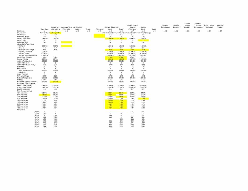
Source Term Averaging Time Wind Speed Surface RoughnessMonin-Obukhov
Length StabilityAmbient
TemperatureAmbient Pressure
Ambient Relative Humidity
Ambient Surface
TemperatureWater Transfer
SubmodelMolecular
WeightBase Case Alternative 1 Alternative Lower Upper Alternative Lower Upper Alternative Lower Upper
Run Name a b a_1 a_2 a_3 a_4 a_5 a_6 a_7 a_8 a_9 a_10 a_11 a_12 a_13 a_14 a_15Source Term m diamter, 10.67k steady state 2m diamter, 10.67km diamter, 10.67km diamter, 10.67km diamter, 10.67kg/sWind Speed 2.3 2.3 2.3 2.3 2.3 2.3Reference Height 10 10 10 10 10 10Surface Roughness 1.00E-02 1.00E-02 2.00E-05 3.00E-02 1.00E-02 1.00E-02Wind Stability F F F F F EAveraging Time 30 30 30 30 30 30Atmospheric Parameters
DELTA Y 0.03702 0.03702 0.03702 0.03702 0.03702 0.05603BETA Y 0.9 0.9 0.9 0.9 0.9 0.9Monin-Obukhov Length 11.8 11.8 4.08 14.3 13.3 30.4Sigma X Coefficient 1.70E-01 1.70E-01 1.70E-01 1.70E-01 1.70E-01Sigma X Power 9.70E-01 9.70E-01 9.70E-01 9.70E-01 9.70E-01Sigma X Minimum Distance 5.00E+01 5.00E+01 5.00E+01 5.00E+01 5.00E+01
Wind Power Constant 0.349 0.349 0.318 0.386 0.334 0.257Friction Velocity 0.07396 0.07396 0.03268 0.08839 0.07709 0.09523Ambient Temperature 286.25 286.25 286.25 286.25 286.25 286.25Ambient Pressure 1 1 1 1 1 1Ambient Relative Humidity 100 100 100 100 100 100Isothermal? N N N N N NHeat Transfer? Y Y Y Y Y Y
Surface Temperature 286.25 285.95 285.95 285.95 285.95 285.95Correlation 1 1 1 1 1 1
Water Transfer? N N N N N NMolecular Weight 57.8 58.7 57.8 57.8 57.8 57.8Release Temperature 286.25 286.25 286.25 286.25 286.25 286.25Density 2.477 2.477 2.477 2.477 2.477 2.477Mean heat capacity constant 586.68 577.28 586.27 586.27 586.27 586.27Mean heat capacity powerUpper Concentration 2.50E-01 2.50E-01 2.50E-01 2.50E-01 2.50E-01 2.50E-01Lower Concentration 1.00E-04 1.00E-04 1.00E-04 1.00E-04 1.00E-04 1.00E-04Height for isopleths 0.5 0.5 0.5 0.5 0.5 0.5Max Concentration at:40m centerline 29.5% 28.2% 12.8% 32.4% 30.0% 26.7%53m centerline 29.5% 28.2% 12.8% 16.0% 28.9% 20.4%72m centerline 12.5% 22.4% 12.8% 11.5% 12.9% 12.4%90m centerline 10.0% 15.2% 12.8% 7.9% 9.9% 7.8%112m centerline 7.0% 8.8% 12.8% 4.6% 6.7% 4.9%158m centerline 3.3% 3.3% 12.8% 1.9% 3.1% 2.1%250m centerline 1.0% 0.9% 3.3% 0.6% 1.0% 0.7%335m centerline 0.5% 0.5% 1.7% 0.3% 0.5% 0.4%472m centerline 0.2% 0.2% 0.8% 0.1% 0.2% 0.2%Distance to:
20.0% 21 78 11 37 33 5412.9% 69 96 33 66 72 718.9% 97 112 199 86 97 856.2% 119 128 199 99 117 1013.8% 150 153 120 145 1242.6% 173 173 283 141 169 1440.8% 282 272 484 224 275 2390.5% 331 321 579 264 327 2880.4% 384 371 663 304 375 335

Thorney Island 47 Measured vs Predicted Maximum Arcwise Concentration
Long Time Average
0.0
10.0
20.0
30.0
40.0
50.0
60.0
70.0
80.0
90.0
100.0
0 100 200 300 400 500 600 700 800 900 1000
Downwind distance (m)
Max
imu
m a
rcw
ise
con
cen
trat
ion
(%
)
Measured
Measured
Measured
Measured
Measured
Measured
Predicted
Predicted
Predicted
Predicted
Predicted
Predicted

Source Term Averaging TimeMonin-Obukhov
LengthAmbient
TemperatureAmbient Pressure
Ambient Relative
Ambient Surface
Water Transfer Submodel
Molecular Weight
Base Case Alternative 1 Alternative Lower Upper Alternative Lower Upper Alternative Lower UpperRun Name a b a_1 a_2 a_3 a_4 a_5 a_6 a_7 a_8 a_9 a_10 a_11 a_12 a_13 a_14 a_15Source Term 2m diamter, 10.2steady state, 2m diamter, 10.22kg/s 2m diamter, 10.22m diamter, 10.22m diamter, 10.22m diamter, 10.22kg/sWind Speed 1.50 1.50 1.50 1.50 1.50 1.50Reference Height 10.00 10.00 10.00 10.00 10.00 10.00Surface Roughness 1.00E-02 1.00E-02 2.00E-05 3.00E-02 1.00E-02 1.00E-02Wind Stability F F F F F EAveraging Time 30.00 30.00 30.00 30.00 30.00 30.00Atmospheric Parameters
DELTA Y 0.04 0.04 0.04 0.04 0.04 0.06BETA Y 0.90 0.90 0.90 0.90 0.90 0.90Monin-Obukhov Length 11.80 11.80 4.08 14.30 10.00 30.40Sigma X Coefficient 1.70E-01 1.70E-01 1.70E-01 1.70E-01 1.70E-01Sigma X Power 9.70E-01 9.70E-01 9.70E-01 9.70E-01 9.70E-01Sigma X Minimum Distance 5.00E+01 5.00E+01 5.00E+01 5.00E+01 5.00E+01
Wind Power Constant 0.349 0.349 0.318 0.386 0.372 0.257Friction Velocity 0.05 0.05 0.02 0.06 0.05 0.06Ambient Temperature 287.45 287.45 287.45 287.45 287.45 287.45Ambient Pressure 1.00 1.00 1.00 1.00 1.00 1.00Ambient Relative Humidity 97.40 97.40 97.40 97.40 97.40 97.40Isothermal? N N N N N NHeat Transfer? Y Y Y Y Y Y
Surface Temperature 287.65 287.65 287.65 287.65 287.65 287.65Correlation 1.00 1.00 1.00 1.00 1.00 1.00
Water Transfer? N N N N N NMolecular Weight 57.80 57.80 57.80 57.80 57.80 57.80Release Temperature 287.45 286.45 287.45 287.45 287.45 287.45Density 2.48 2.51 2.51 2.51 2.51 2.51Mean heat capacity constant 586.68 586.68 586.27 586.27 586.27 586.27Mean heat capacity powerUpper Concentration 20.00% 20.00% 20.00% 20.00% 20.00% 20.00%Lower Concentration 0.20% 0.10% 0.10% 0.10% 0.10% 0.10%Height for isopleths 0.50 0.50 0.50 0.50 0.50 0.50Max Concentration at:50m centerline 17.4% 17.0% 11.0% 20.4% 15.6% 25.1%90m centerline 17.4% 17.0% 9.2% 20.4% 15.6% 9.0%212m centerline 2.0% 6.8% 7.7% 1.3% 1.9% 2.1%250m centerline 1.2% 4.0% 6.9% 0.8% 1.2% 1.2%335m centerline 0.5% 1.4% 0.6% 0.3% 0.5% 0.7%472m centerline 0.2% 0.5% 0.5% 0.1% 0.2% 0.3%Distance to:
15.9% 136 145 19 21 20 827.4% 139 236 236 113 158 1141.5% 237 333 271 196 217 2490.7% 312 441 441 258 294 3350.5% 349 500 500 301 344 3790.2% 456 679 679 384 439 499
Wind Speed Surface Roughness Stability

CHRC A Scaled Measured vs Predicted Maximum Arcwise Concentration
Long Time Average
0.0
10.0
20.0
30.0
40.0
50.0
60.0
70.0
80.0
90.0
100.0
0 100 200 300 400 500 600 700 800 900 1000
Downwind distance (m)
Max
imu
m a
rcw
ise
con
cen
trat
ion
(%
) Measured
Predicted

BA Hamburg DA0120 Scaled Measured vs Predicted Maximum Arcwise Concentration
Long Time Average
0.0
10.0
20.0
30.0
40.0
50.0
60.0
70.0
80.0
90.0
100.0
0 100 200 300 400 500 600 700 800 900 1000
Downwind distance (m)
Max
imu
m a
rcw
ise
con
cen
trat
ion
(%
)
Measured
Measured
Measured
Measured
Measured
Measured
Measured
Measured
Predicted
Predicted
Predicted
Predicted
Predicted
Predicted
Predicted
Predicted

BA Hamburg DAT223 Scaled Measured vs Predicted Maximum Arcwise Concentration
Long Time Average
0.0
10.0
20.0
30.0
40.0
50.0
60.0
70.0
80.0
90.0
100.0
0 100 200 300 400 500 600 700 800 900 1000
Downwind distance (m)
Max
imu
m a
rcw
ise
con
cen
trat
ion
(%
)
Measured
Measured
Measured
Predicted
Predicted
Predicted

BA TNO FLS Scaled Measured vs Predicted Maximum Arcwise Concentration
Long Time Average
0.0
10.0
20.0
30.0
40.0
50.0
60.0
70.0
80.0
90.0
100.0
0 100 200 300 400 500 600 700 800 900 1000
Downwind distance (m)
Max
imu
m a
rcw
ise
con
cen
trat
ion
(%
) Measured
Predicted

APPENDIX B: REFERENCES

REFERENCES
AcuTech Consulting Group (2009). Final Report: Review of the LNG Vapor Dispersion Model Evaluation Protocol. The National Association of State Fire Marshals.
Blackmore, D.R., Eyre, J.A., Summers, G.G. (1982), Dispersion and Combustion Behaviour of Gas Clouds Resulting from Large Spillages of LNG and LPG on the Sea. Transactions of the Institute of Marine Engineers, Volume 94, Paper 92, 1982. Institute of Marine Engineers.
Blackmore, D.R., Colenbrander, G.W., Puttock, J.S., (1984). Maplin Sands Experiments 1980: Dispersion of Refrigerated Liquid Propane and LNG, NATO Challendges of Modern Society—Air Pollution Modelling and Its Application 3, Volume 5, Pages 353-373, Plenum, New York, USA.
Brutstaert, W. (1982). Evaporation into the Atmosphere: Theory, History, and Applications. Kluwer Academic Publishers, Netherlands.
Coldrick, S., Lea, C.J., Ivings, M.J. (2010). Validation Database for Evaluating Vapor Dispersion Models for Safety Analysis of LNG Facilities, Version 11.0. The Fire Protection Research Foundation, Quincy, Massachusetts.
Colenbrander, G.W., (1980). A Mathematical Model for the Transient Behavior of Dense Vapor Clouds, 3rd International Symposium on Loss Prevention and Safety Promotion in the Process Industries, Basel, Switzerland, 1980.
Colenbrander, G.W., Evans, A., Puttock, J.S. ( 1983). Dense Gas Dispersion Behavior: Experimental Observations and Model Developments. International Symposium on Loss Prevention and Safety Promotion in the Process Industries, Harrogate, England, September 1983.
Colenbrander, G.W., Evans, A., Puttock, J.S. (1984a). Spill Tests of LNG and Refrigerated Liquid Propane on the Sea, Maplin Sands, 1980: Dispersion Data Digest; Trial 27. Shell Research Limited, TNER.84.028.
Colenbrander, G.W., Evans, A., Puttock, J.S. (1984b). Spill Tests of LNG and Refrigerated Liquid Propane on the Sea, Maplin Sands, 1980: Dispersion Data Digest; Trial 34. Shell Research Limited, TNER.84.030.
Colenbrander, G.W., Evans, A., Puttock, J.S. (1984c). Spill Tests of LNG and Refrigerated Liquid Propane on the Sea, Maplin Sands, 1980: Dispersion Data Digest; Trial 35. Shell Research Limited, TNER.84.031.
Eyre, J.A., Hirst, W.J.S. (1983), Maplin Sands Experiments 1980: Combustion of Large LNG and Refrigerated Liquid Propane Spills on the Sea. Proceedings, 2nd Symposium on Heavy Gas and Risk Assessment II, West Germany, May 25-26, 1983, D Reidel Publishing Company, Netherlands.

REFERENCES (cont’d)
Ermak, D.L, Chapman, R., Goldwire, H.C., Gouveia, F.J., Rodean, H.C. (1989). Heavy Gas Dispersion Test Summary Report. Lawrence Livermore National Laboratory.
Federal Energy Regulatory Commission (FERC) (2004a). Consequence Assessment Methods for Incidents Involving Releases from Liquefied Natural Gas Carriers. Docket No. AD04-6-000.
Federal Energy Regulatory Commission (FERC) (2004b). Staff’s Responses to Comments on the Consequence Assessment Methods for Incidents Involving Releases from Liquefied Natural Gas Carriers. Docket No. AD04-6-000.
Havens, J., (1982),Dispersion of Dense Vapors, Volume 2, MIT-GRI LNG Safety and Research Workshop. GRI 82/0019.2, Gas Research Institute (GRI).
Havens, J., Spicer, T.O., (1985), Development of an Atmospheric Dispersion Model for Heavier-Than-Air Gas Mixtures, Volume 1, Final Report Contract DT-CG-23-80-C-20029, United States Coast Guard, Washington, D.C.
Havens, J., (1988), A Dispersion Model for Elevated Dense Gas Jet Chemical Releases, Volume 1, EPA 450/4-88-006a, Environmental Protection Agency.
Havens, J., Spicer, T. ( 1990). LNG Vapor Dispersion Prediction with the DEGADIS Dense Gas Dispersion Model. Report GRI 89/0242, Gas Research Institute (GRI), 1990.
Gavelli, F., Davis, S.G., Hansen, O.H., (2011), User Beware: When Simple Consequence Models Can Give the Wrong Answers, Proceedings of AIChE Spring Meeting, 7th Global Congress on Process Safety, Chicago, IL, March 16, 2011.
Goldwire, H.C., Rodean, H.C., Cederwall, R.T., Kansa, E.J., Koopman, R.P., McClure, J.W., McRae, T.G., Morris, L.K., Kamppinen, L., Kiefer, R.D., Urtiew, P.A., Lind, C.D. (1983a). Coyote Series Data Report LLNL/NWC 1981 LNG Spill Tests, Dispersion, Vapor Burn, and Rapid Phase Transition. Lawrence Livermore National Laboratory, UCID-19953, Volume 1.
Goldwire, H.C., Rodean, H.C., Cederwall, R.T., Kansa, E.J., Koopman, R.P., McClure, J.W., McRae, T.G., Morris, L.K., Kamppinen, L., Kiefer, R.D., Urtiew, P.A., Lind, C.D. (1983b). Coyote Series Data Report LLNL/NWC 1981 LNG Spill Tests, Dispersion, Vapor Burn, and Rapid Phase Transition. Lawrence Livermore National Laboratory, UCID-19953, Volume 2.
Hanna, S.R., Strimaitis, D.G., Chang, J.C. (1993). Final Report: Hazard Response Modeling Uncertainty (A Quantitative Method), Vol II - Evaluation of Commonly Used Hazardous Gas Dispersion Models. Air Force Engineering & Services Center, Environics Division, AD-A270-095, ESL-TR-91-28.
REFERENCES (cont’d)
Ivings, M.J., Jagger, S.F., Lea, C.J., Webber, D.M. (2007). Evaluating Vapor Dispersion Models for Safety Analysis of LNG Facilities. The Fire Protection Research Foundation, Quincy, Massachusetts.
Johnson, D.R. (1985), Thorney Island: Its Geography and Meteorology, Heavy Gas Dispersion Trials at Thorney Island, Proceedings of a Symposium held at University of Sheffield, Great Britain, April 3-5, 1984, Elsevier, 1985.
Kantha, H.L., Phillips, O.M., Azad, R.S. (1977), On Turbulent Entrainment at a Stable Density Interface. Journal of Fluid Mechanics, Vol. 79, pp 753-768.
Koopman, R.P, Cederwall, R.T., Ermak, D.L., Goldwire, H.C., McClure, J.W., McRae, T.G., Morgan, D.L., Rodean, H.C., Shinn, J.H. (1981). Description and Analysis of Burro Series 40-m3 LNG Spill Experiments. Lawrence Livermore National Laboratory, UCRL-53186.
Koopman, R.P, Baker, J., Cederwall, R.T., Goldwire, H.C., Hogan, W.J., Kamppinen, L.M., Kiefer, R.D., McClure, J.W., McRae, T.G., Morgan, D.L., Morris, L.K., Spann, M.W., Lind, C.D. (1982a). Burro Series Data Report LLNL/NWC 1980 LNG Spill Tests. Lawrence Livermore National Laboratory, UCID-19075, Volume 1.
Koopman, R.P, Baker, J., Cederwall, R.T., Goldwire, H.C., Hogan, W.J., Kamppinen, L.M., Kiefer, R.D., McClure, J.W., McRae, T.G., Morgan, D.L., Morris, L.K., Spann, M.W., Lind, C.D. (1982b). Burro Series Data Report LLNL/NWC 1980 LNG Spill Tests, The Appendices. Lawrence Livermore National Laboratory, UCID-19075, Volume 2.
Koopman, R.P, Cederwall, R.T., Ermak, D.L., Goldwire, H.C., Hogan, W.J., McClure, J.W., McRae, T.G., Morgan, D.L., Rodean, H.C., Shinn, J.H. (1982c). Analysis of Burro Series 40-m3 LNG Spill Experiments. Journal of Hazardous Materials, Vol 6.
Leck, M.J., Lowe, D.J., (1985). Development and Performance of the Gas Sensor System, Hevay Gas Dispersion Trials at Thorney Island, Proceedings of a Symposium held at University of Sheffield, Great Britain, April 3-5, 1984, Elsevier, 1985.
Lofquist, K. (1960), Flow and Stress Near an Interface Between Stratified Liquids. Physics of Fluids, Vol 3. No. 2. March-April 1960.
McQuaid, J. (1976), Some Experiments on the Sztructure of Stably Stratified Shear Flows, Technical Paper P21, Safety in Mine Research Establishment, Sheffield, UK, 1976.

REFERENCES (cont’d)
Melton, T.A., Cornwell, J.B. (2009). LNG Trench Dispersion Modeling Using Computational Fluid Dynamics. 12th Annual Symposium, Mary Kay O’Connor Process Safety Center.
Nussey, C., Davies, J.K.W., Mercer, A.,(1985). The Effect of Averaging Time on the Statistical Properties of Sensor Records, Hevay Gas Dispersion Trials at Thorney Island, Proceedings of a Symposium held at University of Sheffield, Great Britain, April 3-5, 1984, Elsevier, 1985.
Pielke, R.A., (2002). Mesoscale Meteorological Modeling, 2nd Edition, Academic Press, New York, 2002.
Pipeline and Hazardous Materials Safety Administration, U.S. Department of Transportation (PHMSA) (2010). Advisory Bulletin ADB-10-07 Liquefied Natural Gas Facilities: Obtaining Approval of Alternative Vapor-Gas Dispersion Models. Federal Register 75 (August 31, 2010): 53371-53374.
Puttock, J.S, Colenbrander, G.W., (1980) Maplin Sands Experiments 1980: Interpretation and Modeling of Liquefied Gas Spills onto the Sea. IUTAM Symposium on Atmosphere Dispersion of Heavy Gases and Small Particles, Delft, West Germany, August/September 1983, Springer-Verlag, Berlin, West Germany.
Puttock, J.S., Blackmore, D.R., Colenbrander, G.W., Davies, P.T., Evans, A., Homer, J.B., Redfearn, J.J., Vant Sant, W.C., Wilson, R.P. (1984). Spill Tests of LNG and Refrigerated Liquid Propane on the Sea, Maplin Sands, 1980: Experimental Details of the Dispersion Tests. Shell Research Limited, TNER.84.046.
Puttock, J. (1987). The Development and Use of HEGABOX/HEGADIS Dispersion Models for Hazard Analysis. Proceedings, International Conference on Vapour Cloud Modeling, pp. 317-341.
Research and Special Programs Administration (RSPA) (1997). Direct Final Rule: Liquefied Natural Gas Regulations - Miscellaneous Amendments. Federal Register 62 (February 25, 1997): 8403-8404.
Spicer, T.O., Havens, J., (1989). User’s Guide for the DEGADIS 2.1 Dense Gas Dispersion Model, EPA-450/4-89-019, Environmental Protection Agency, Research Triangle Park, NC, November 1989.
Zeman, O. Tennekes, H. (1977), Parameterization of the Turbulent Energy Budget at the Top of the Daytime Atmospheric Boundary Layer, Journal of the Atmospheric Sciences, January 1977.

APPENDIX C: LIST OF PREPARERS

LIST OF PREPARERS
Kohout, Andrew - Federal Energy Regulatory Commission B.S., Mechanical Engineering, 2006, University of Maryland B.S., Fire Protection Engineering, 2006, University of Maryland