Evaluation of Causal Discovery Models inBivariate Case Using Real World Data

Jing Song, Satoshi Oyama, Haruhiko Sato, and Masahito Kurihara

Abstract—Causal relationships are different from statisticalrelationships. Distinguishing cause from effect is a fundamentalscientific problem that has attracted the interest of manyresearchers. Among causal discovery problems, discoveringbivariate causal relationships is a special case because the well-known independent tests are useless. We empirically testedthree existing state-of-the-art models, ANM, PNL model, andIGCI model, for causal discovery in the bivariate case usingreal world data and compared their performance using threemetrics: accuracy, area under ROC curve (AUC), and timecost to make a decision. We concluded the strong points andweaknesses of each method through our experiments. For theefficiency of algorithm, we found that the IGCI model is thefastest even when the dataset is large and that the PNL modelcosts the most time to give a decision.

Index Terms—causal discovery, bivariate, accuracy, areaunder curve, time cost.

I. INTRODUCTION

People are generally more concerned with causal rela-tionships between variables than they are with statisticalrelationships between variables, and “causality” [1], [2], [3],[4] has attracted the interest of researchers in various fields,including economics, sociology, and machine learning. Thebest way to verify causal relationship between variables isto conduct a controlled experiment. However, in the realworld, such experiments are often too expensive, unethi-cal, or even impossible. Many researchers are thus usingstatistical methods to analyze causal relationships betweenvariables [5], [6], [7], [8]. Some concepts of causality havebeen formalized using directed acyclic graphs. As a generalalgorithm for causal discovery, a conditional independencetest can be used to exclude irrelevant relationships betweenvariables [3], [4]. However, in the case of two variables, aconditional independence test is impossible. Several modelshave been proposed to solve this problem [9], [10], [11],[12], [13], [14], [15].

For two variables X and Y, there are four possible re-lationships, besides independence and feedback, betweenthem (Figure 1). The top two diagrams in Figure 1 showthe possible causal relationships between X and Y. Theremaining task is to decide the direction of the arrow. Thebottom two diagrams represent the “common cause” (left)and “selection bias” (right) case. The unobserved variablesZ are “confounders”1 for causal discovery between X andY. The existing of “confounders”2 will bring spurious cor-relation between X and Y. How to distinguish spurious

The authors are in the Division of Computer Science and In-formation Technology in the Graduate School of Information Sci-ence and Technology, Hokkaido University, Sapporo, Japan, 060-0814. Email:songjing@complex.ist.hokudai.ac.jp, oyama@ist.hokudai.ac.jp,haru@complex.ist.hokudai.ac.jp, kurihara@ist.hokudai.ac.jp

1For the definition of confouding, please refer to [16], [17].2The number of “confounders” is not limited to one.

Fig. 1. Four Possible Relationships between X and Y (Besides Indepen-dence and Feedback).

correlation with “confounders” from actual causality is aremaining challenging task in this field. Many current modelsare based on the assumption that “confounders” do not exist.3

We compared the performance of three existing state-of-the-art models, ANM, PNL and IGCI, under the assumption thatconfounders do not exist. We used three metrics: accuracy,area under ROC curve (AUC), and time cost to make adecision.

In section II, we introduce some related work in causaldiscovery. In section III, we briefly introduce the threemodels: ANM, PNL and IGCI. In section IV, we describe thedataset we used and the implementation of the three models.In section V, we present the results and give a detailedanalysis of the performance of the three models. We concludein section VI by summarizing the advantages and weaknessesof the three models and mentioning future tasks.

II. RELATED WORK

Granger causality [6] is proposed to detect causal directionof time series data based on temporal ordering of variables.Granger causality only works on the linear stochastic sys-tems. Chen et al. [21] extends the model to work on nonlinearsystems. For Granger causality [6] and extended Grangercausality [21], temporal information is needed.

Shimizu et al. [18] proposed the LiNGAM (short for linearnon-gaussian acyclic model) which can detect causal direc-tion of varialbes no matter whether temporal informationis available or not. The LiNGAM works when the causalrelationship between variables is linear, the distributionsof disturbance variables are non-Gaussian and the networkstructure can be expressed using DAG (short for directed

3Dealing with confounders is an on-going work in this field. As far as weknow, Shimizu et al. extend the LiNGAM [18] to detect causal directionwhen “common causes” exist [19], [20]. However, many current modelswork under the assumption that no confounders exist.

Proceedings of the International MultiConference of Engineers and Computer Scientists 2016 Vol I, IMECS 2016, March 16 - 18, 2016, Hong Kong

ISBN: 978-988-19253-8-1 ISSN: 2078-0958 (Print); ISSN: 2078-0966 (Online)

IMECS 2016

acyclic graph). Some extensions of LiNGAM has beenproposed [22], [19], [23], [20].

LiNGAM is based on the assumption of linear relation-ships between variables. Hoyer et al. [12] propose additive-noise model (ANM) to deal with non-linear relationships.When the regression function is linear, ANM works in thesame way as LiNGAM. Zhang et al. propose the post non-linear (PNL) model which takes into account the nonlineareffect of causes, additive inner noise and external sensordistortion. A brief introduction of ANM and PNL will begiven in section III.

The above methods are based on the structural equationmodeling (SEM) which requires structural constraints onthe data generating process. Another research direction isbased on the assumption of independent mechanisms ofnature to generate causes and effects. The idea is that theshortest description of joint distribution p(cause, effect)can be expressed by p(cause)p(effect|cause). Comparedwith p(effect)p(cause|effect), p(cause)p(effect|cause)has lower total complexity.

Janzing et al. [14], [15] propose information geometriccausal inference (IGCI) model to infer asymmetry betweencause and effect through the complexity loss of distributions.A brief introduction of IGCI will be given in the followingsection. Zhang et al. [24] propose a bootstrap-based approachto detect causal direction based on the condition that theparameters of the cause involved in the causality data gen-erating process is exogenous from that of the cause to theeffect. Mooij et al. [11] propose a probabilistic latent variablemodel (GPI) to distinguish between cause and effect usingstandard Bayesian model selection.

In the above work, accuracy is usually used to evaluatethe performance of causal discovery models. Besides ofaccuracy, we use an evaluation method for a binary classifier:area under ROC curve (AUC) as another evaluation methodin our work. We compare existing methods using threemetrics: accuracy, AUC, and time cost to make a decision.

III. MODELS

The three models we choose in our experiments werethe additive-noise model (ANM) [12], the post non-linear(PNL) model [13], [25], and the information geometriccausal inference (IGCI) model [14], [15]. The three modelsare typical and state-of-the-art models for causal discovery inbivariate case. The first two models define how causality datais generated in nature. The last model finds the asymmetrybetween cause and effect through the complexity loss ofdistributions.

A. ANM

The additive noise model (ANM) of Hoyer et al. [12]is based on two assumptions: the observed effects can beexpressed using functional models of the cause and additivenoise (Equation 1) and the cause and additive noise areindependent. If f() is a linear function and the noise has anon-Gaussian distribution, ANM works in the same way asthe linear non-Gaussian acyclic model (LiNGAM) [18]. Themodel is learned by performing regression in both directionsand calculating the independence between the assumed causeand noise (residuals) for each direction. The decision rule

is to choose the direction with the larger independenceas the true causal direction. ANM cannot deal with thelinear Gaussian case since the data can fit the model inboth directions, so the asymmetry between cause and effectdisappears. In [26], Gretton et al. improved the algorithmand extended ANM to work even in the linear Gaussiancase [26]. The improved model also works more efficientlyin the multivariate case.

effect = f(cause) + noise (1)

B. PNL Model

In the post-nonlinear (PNL) model of Zhang et al. [13],[25], effects are nonlinear transformations of causes withsome inner additive noise, followed by an external nonlineardistortion (Equation 2). From Equation 2, we can get thatnoise = f2

−1(effect)− f1(cause), where cause and effectare the two observed variables. To identify the cause andeffect, nonlinear independent component analysis (ICA) isperformed to extract two components that are as independentas possible. The extracted components should be independentfor the true direction. The validity of the PNL model has beenproven [25].

effect = f2(f1(cause) + noise) (2)

C. IGCI Model

The IGCI model [14], [15] is based on the hypothesisthat if “X causes Y,” the marginal distribution p(x) andthe conditional distribution p(y|x) are independent. TheIGCI model gives an information-theoretic view of additivenoise and defines independence by using orthogonality. Withthe ANM [12], if there is no additive noise, inference isimpossible while it is possible with the IGCI model.

The IGCI model determines the causal direction on thebasis of complexity loss. Let νx and νy be the referencedistributions for X and Y. D(Px || νx) :=

∫log P (x)

ν(x)P (x)dx

is the KL-distance between Px and νy , which works as afeature of the complexity of the distribution. The complexityloss from X to Y can be defined by

VX→Y := D(Px || νx)−D(Py || νy). (3)

The decision rule of the IGCI model is that, if VX→Y < 0,infer “X causes Y,” else if VX→Y > 0 infer “Y causes X.”This rule is rather theoretical. An applicable and explicit formfor the reference measure is entropy-based IGCI or slope-based IGCI.

1) Entropy-based IGCI:

S(PX) := ψ(m)− ψ(1) + 1

m− 1

m−1∑i=1

log|xi+1 − xi|

(4)

VX→Y := S(PY )− S(PX) = −VY→X (5)

2) Slope-based IGCI:

VX→Y :=1

m− 1

m−1∑i=1

log

∣∣∣∣ yi+1 − yixi+1 − xi

∣∣∣∣ (6)

Proceedings of the International MultiConference of Engineers and Computer Scientists 2016 Vol I, IMECS 2016, March 16 - 18, 2016, Hong Kong

ISBN: 978-988-19253-8-1 ISSN: 2078-0958 (Print); ISSN: 2078-0966 (Online)

IMECS 2016

The explicit form of IGCI is simpler, and we can seethat the two IGCI models coincide with each other. Thecalculation does not cost much time even when dealing withbig data. However, the IGCI model prefers low-noise dataand may perform poorly in a high-noise situation. We discussthe strengths and weaknesses of the IGCI model in sectionV.

IV. EXPERIMENTS

In this section, we describe the data used in our experi-ments and the implementation of each model. The results arepresented in section V.

A. Dataset

We used the CauseEffectPairs (CEP) [27] dataset, whichcontains 97 pairs of real world causal variables with thegold standard labeled for each pair. The data set is publiclyavailable online [27]. Some of the data were collected fromthe UCI Machine Learning Repository [28]. The data comesfrom various fields, including geography, biology, physics,and economics. The dataset also contains time series data.Most of the data contains much noise. An appendix containsa detailed description of each pair of variables [29].

We used 91 of the pairs in our experiments since someof the data (e.g, pair0052) in CEP [27] contains multi-dimentional variables4. Scatter plots of the data are shown inFigure 2. The variables range in size from 126 to 16,382. Thevariety of data types makes causal analysis using real worlddata challenging. Moreover, the dataset is not well balanced:of the 91 pairs, the true label is “X causes Y” for 67 pairsand “Y causes X” for the other 24 pairs.

B. Implementation Details

We implemented the three models as described in theoriginal work.

a) ANM: Using the reported experiment settings [12],we performed Gaussian processes for machine learningregression [30], [31]. We then used the Hilbert-SchmidtIndependence Criterion (HSIC) [32] to test the independencebetween the assumed cause and residuals. The dataset usedhad been labeled with the true causal direction for each pairwith no independence, or feedback. Using the decision ruleof ANM, we determined that the direction with the greaterindependence was the true causal direction.

b) PNL: We used nonlinear ICA to extract the twocomponents that were assumed to be the cause and noiseif the model had been learned in the right direction. Thenonlinearities of f1 and f2−1 in Equation 2 were modeled bymulti-layer perceptrons. By minimizing the mutual informa-tion between the two output components, we made the outputas independent as possible. After extracting two independentcomponents, we tested their independence by using HSIC[32]. Finally, in the same way as for ANM, we determinedthat the direction with the greater independence was the trueone.

4The three models we implemented in our experiment cannot deal withmulti-dimentional data.

Fig. 2. Scatter Plot of Data Used in Experiments

c) IGCI(entropy,uniform): Compared with the othertwo models, the implementation of the IGCI model is sim-pler. We used reported equations (4, 5) to calculate VX→Yand VY→X and determined that the direction in whichentropy decreased was the true direction. If VX→Y < 0,the inferred causal direction was “X causes Y”; otherwise,it was “Y causes X.” For the IGCI model, the data shouldbe normalized before calculating VX→Y and VY→X . Inaccordance with the reported experiment results, we used theuniform distribution as the reference distribution because ofits good performance. For the repetitive data in the dataset,we set log0 = 0.

d) IGCI(slope,uniform): The implementation of theIGCI(slope, uniform) model was similar to that of theIGCI(entropy, uniform) one. We used (6) to calculate VX→Yand VY→X and determined that the direction with a negativevalue was the true one. For the same reason as above,we mapped the data to [0,1] before calculating VX→Y andVY→X . To make (6) meaningful, we filtered out the repetitivedata.

V. RESULTS

Here, we first compare model accuracy for different deci-sion rates. We changed the threshold continually and calcu-lated the corresponding accuracy for each model. Althoughthe accuracy of the models for different decision rates hasbeen compared elsewhere, we used more real world data inour experiments. In addition, we wanted to compare the per-formance of the models using different evaluation methods.The performance of the models for different decision ratesis discussed in subsection V-A.

Proceedings of the International MultiConference of Engineers and Computer Scientists 2016 Vol I, IMECS 2016, March 16 - 18, 2016, Hong Kong

ISBN: 978-988-19253-8-1 ISSN: 2078-0958 (Print); ISSN: 2078-0966 (Online)

IMECS 2016

Since causal discovery models in the bivariate case give adecision between two choices, we can regard these modelsas binary classifiers and evaluate them using the area underROC curve (AUC). Although there is difference betweenthe outputs of the three models and a binary classifier, wepropose a way to overcome this problem. It is described insubsection V-B.

Finally, we compare model efficiency by calculating theaverage time needed to give a decision. This is described insubsection V-C.

A. Accuracy For Different Decision Rates

We calculated the accuracy of each model for differentdecision rates using (7) and (8) and plotted the results(Figure 3). The decision rate changed when the thresholdwas changed. The larger the threshold, the more stringentthe decision rule. In an ideal situation, accuracy decreasesas the decision rate increases, with the starting point at 1.0.However, the results with real world data were not perfectbecause there was much noise in the data.

As shown in Figure 3, the accuracy started from 1.0 for theANM and IGCI model and from 0.0 for the PNL model. Thismeans that the PNL model gave the wrong decision when ithad the highest confidence. Investigation showed that PNLmodel made a wrong decision with the highest confidencebecause of the discretization of data5. Besides, we can seethat, although the accuracy of the IGCI model started from1.0, the accuracy dropped sharply when the decision ratewas between 0.0 and 0.2. The reason why accuracy dropsis that IGCI made wrong decisions with large confidencewhen dealing with pair0056-pair0063. These eight pairs ofvariables contain much noise which makes IGCI give badperformance. Besides, there are some “outliers” for the eightpairs which affect the decision result much6. After reachinga minimum, the accuracy increased continuously and becamemore stable. Compared with the other models, the accuracyof ANM was relatively stable with a starting value of 1.0.When all decisions have been made, the accuracies of thesemodels are ranked IGCI > ANM > PNL.

DecisionRate :=NDecisionNData

(7)

Accuracy :=NTrueDecisionNDecision

(8)

B. Area Under ROC Curve (AUC)

Besides calculating the accuracy of the three models fordifferent decision rates, we used the area under ROC curve(AUC) to evaluate their performance.

As described in IV-A, the dataset is not well balanced.Although the three models did not train a classifier from thedata, the inference method can be seen as a binary classifier.For a binary classifier, a well- known evaluation method isthe area under ROC curve (AUC). The ROC curve is plotted

5PNL makes wrong decision with the largest confidence when dealingwith pair0070 in [27]. One variable of pair0070 contains only two values:0 and 1. The variable is easy to be inferred as the cause according to themechanism of PNL model.

6This is because that the calculation methods of IGCI (Equation 4,5,6) issusceptible to “outliers”.

Fig. 3. Accuracy of Three Models for Different Decision Rates.

Fig. 4. Process to Label Every Pair of Variables.

by calculating the true positive rate (TPR) and false positiverate (FPR) for different thresholds. The output of a binaryclassifier is a value in the interval [0,1]. In contrast, for thethree models evaluated here, the outputs were the two valuescalculated for the two possible causal directions. Despite thisdifference, we used the following steps to get the ROC curveand at the same time not break the decision rule of the threemodels.

1) Divide the data into two groups: a) inferred as “Xcauses Y” and b) inferred as “Y causes X” in accor-dance with the decision rule of the model.

2) Let VX−>Y and VY−>X be the outputs of the models.Calculate the absolute value of the difference betweenVX−>Y and VY−>X (Equation 9) and map Vdif to[0,1].

3) Label every pair of data in accordance with the processdiagrammed in Figure 4.

4) Use Vdif and the generated labels in 1) to calculate theTPR and FPR for different thresholds. Plot the ROCcurve and calculate the corresponding AUC value.

Vdif = |VX−>Y − VY−>X | (9)

In step 1), we divided the data into two groups because the

Proceedings of the International MultiConference of Engineers and Computer Scientists 2016 Vol I, IMECS 2016, March 16 - 18, 2016, Hong Kong

ISBN: 978-988-19253-8-1 ISSN: 2078-0958 (Print); ISSN: 2078-0966 (Online)

IMECS 2016

basic rule of causal discovery models needs to be observed.For example, we cannot use the division of VX−>Y andVY−>X in the same way as the output of a binary classifier.If we did, the decision rule of the models would be brokenif the threshold was set very large or small. However, ifwe divide the data into two groups in accordance with thedecision result, we not only take into consideration differentlevels of punishment but also observe the original decisionrule.

In step 2), we used the absolute value of the differencebetween VX−>Y and VY−>X as the “confidence” of themodel when giving a decision. The larger the Vdif , thegreater the confidence. We did not use division because, ifone of VX−>Y and VY−>X was very small, the divisionresult would be very large. We mapped Vdif to [0,1] tomake the calculation more convenient. In this way, Vdifcould be used in the same way as the output of a binaryclassifier. For causal discovery, the larger the Vdif , the greaterthe confidence in the decision. At the same time, morepunishment should be given when the decision is wrong.

In step 3), we labeled the data in accordance with thediagram in Figure 4. For the decision “X causes Y,” thepositive class was “X causes Y.” We checked the datasetto see whether the true label was “X causes Y.” If it was,the data was labeled as a positive class, otherwise it waslabeled as a negative class. The same process was done withthe decision “Y causes X”; however, the label was oppositesince in this group “Y causes X” is the positive class.

In step 4), we used the normalized Vdif as the confidenceof a decision and the label assigned in step 3) to calculateTPR and FPR for different thresholds. We plotted TPR andFPR to get the ROC curve and calculated the correspondingAUC value.

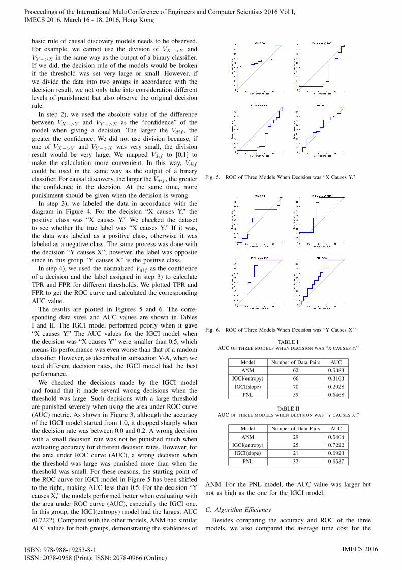
The results are plotted in Figures 5 and 6. The corre-sponding data sizes and AUC values are shown in TablesI and II. The IGCI model performed poorly when it gave“X causes Y.” The AUC values for the IGCI model whenthe decision was “X causes Y” were smaller than 0.5, whichmeans its performance was even worse than that of a randomclassifier. However, as described in subsection V-A, when weused different decision rates, the IGCI model had the bestperformance.

We checked the decisions made by the IGCI modeland found that it made several wrong decisions when thethreshold was large. Such decisions with a large thresholdare punished severely when using the area under ROC curve(AUC) metric. As shown in Figure 3, although the accuracyof the IGCI model started from 1.0, it dropped sharply whenthe decision rate was between 0.0 and 0.2. A wrong decisionwith a small decision rate was not be punished much whenevaluating accuracy for different decision rates. However, forthe area under ROC curve (AUC), a wrong decision whenthe threshold was large was punished more than when thethreshold was small. For these reasons, the starting point ofthe ROC curve for IGCI model in Figure 5 has been shiftedto the right, making AUC less than 0.5. For the decision “Ycauses X,” the models performed better when evaluating withthe area under ROC curve (AUC), especially the IGCI one.In this group, the IGCI(entropy) model had the largest AUC(0.7222). Compared with the other models, ANM had similarAUC values for both groups, demonstrating the stableness of

Fig. 5. ROC of Three Models When Decision was “X Causes Y.”

Fig. 6. ROC of Three Models When Decision was “Y Causes X.”

TABLE IAUC OF THREE MODELS WHEN DECISION WAS “X CAUSES Y.”

Model Number of Data Pairs AUC

ANM 62 0.5383

IGCI(entropy) 66 0.3163

IGCI(slope) 70 0.2928

PNL 59 0.5468

TABLE IIAUC OF THREE MODELS WHEN DECISION WAS “Y CAUSES X.”

Model Number of Data Pairs AUC

ANM 29 0.5404

IGCI(entropy) 25 0.7222

IGCI(slope) 21 0.6923

PNL 32 0.6537

ANM. For the PNL model, the AUC value was larger butnot as high as the one for the IGCI model.

C. Algorithm Efficiency

Besides comparing the accuracy and ROC of the threemodels, we also compared the average time cost for the

Proceedings of the International MultiConference of Engineers and Computer Scientists 2016 Vol I, IMECS 2016, March 16 - 18, 2016, Hong Kong

ISBN: 978-988-19253-8-1 ISSN: 2078-0958 (Print); ISSN: 2078-0966 (Online)

IMECS 2016

TABLE IIITIME COST TO MAKE A DECISION

Model Time Cost

ANM 10.7± 7.4s

PNL 80.5± 19.5s

IGCI(entropy) 0.0014± 0.0019s

IGCI(slope) 0.0014± 0.0017s

algorithm to give a decision. We performed the experimenton the MATLAB platform with an Intel Core i7-4770 3.40GHz2 CPU and 8.00 GB memory. From Table III, we can seethat the IGCI model was the most efficient one while the PNLmodel was the least efficient. ANM was in the middle. Thehigh time cost of the PNL model was due to the modelingnonlinearity of f2−1 and f1 in Equation 2.

VI. CONCLUSION

We compared three existing state-of-the-art models (ANM,PNL model, IGCI model) for causal discovery in the binarycase with real world data. Testing using different decisionrates showed that the IGCI model had the best performance.To check whether the decisions made were reasonable, weused a binary classifier metric: the area under ROC curve(AUC). The IGCI model had a small AUC value for thedecision “X causes Y” because it made several wrongdecisions when the threshold was high. Compared with theother models, the ANM results were relatively stable. Finally,we compared the time cost when making a decision. TheIGCI model was the fastest even when the dataset was large.The PNL model cost the most time to give a decision.

Of the three models, the IGCI one had the best perfor-mance when there was little noise and the data were notdiscretized much. Improving the performance of the IGCImodel when there is much noise and how to deal withdiscretized data are future tasks. Although the performanceof ANM was relatively stable, overfitting should be avoidedfor ANM. Of the three models, the PNL model is the mostgeneralized one as it takes into account the nonlinear effectof causes, additive inner noise, and external sensor distortion.However, modeling the nonlinearities of f1 and f2

−1 takesmuch time for the PNL model.

ACKNOWLEDGMENTS

This work was supported by a grant in aid from JapanSociety for the Promotion of Science (15K1214805).

REFERENCES

[1] C. W. Granger, “Some recent development in a concept of causality,”Journal of econometrics, vol. 39, no. 1, pp. 199–211, 1988.

[2] J. Y. Halpern, “A modification of the halpern-pearl definition ofcausality,” arXiv preprint arXiv:1505.00162, 2015.

[3] P. Spirtes, C. N. Glymour, and R. Scheines, Causation, prediction, andsearch. MIT press, 2000, vol. 81.

[4] J. Pearl, “Causality: models, reasoning, and inference,” EconometricTheory, vol. 19, pp. 675–685, 2003.

[5] D. Janzing, T. MPG, and B. Scholkopf, “Causality: Objectives andassessment,” 2010.

[6] C. W. Granger, “Investigating causal relations by econometric modelsand cross-spectral methods,” Econometrica: Journal of the Economet-ric Society, pp. 424–438, 1969.

[7] B. Scholkopf, D. Janzing, J. Peters, E. Sgouritsa, K. Zhang,and J. Mooij, “On causal and anticausal learning,” arXiv preprintarXiv:1206.6471, 2012.

[8] D. Lopez-Paz, K. Muandet, B. Scholkopf, and I. Tolstikhin, “Towardsa learning theory of cause-effect inference,” in Proceedings of the 32ndInternational Conference on Machine Learning, JMLR: W&CP, Lille,France, 2015.

[9] X. Sun, D. Janzing, and B. Scholkopf, “Distinguishing betweencause and effect via kernel-based complexity measures for conditionaldistributions.” in ESANN, 2007, pp. 441–446.

[10] D. Janzing, P. O. Hoyer, and B. Scholkopf, “Telling cause fromeffect based on high-dimensional observations,” arXiv preprintarXiv:0909.4386, 2009.

[11] O. Stegle, D. Janzing, K. Zhang, J. M. Mooij, and B. Scholkopf,“Probabilistic latent variable models for distinguishing between causeand effect,” in Advances in Neural Information Processing Systems,2010, pp. 1687–1695.

[12] P. O. Hoyer, D. Janzing, J. M. Mooij, J. Peters, and B. Scholkopf,“Nonlinear causal discovery with additive noise models,” in Advancesin neural information processing systems, 2009, pp. 689–696.

[13] K. Zhang and A. Hyvarinen, “Distinguishing causes from effects usingnonlinear acyclic causal models,” in Journal of Machine Learning Re-search, Workshop and Conference Proceedings (NIPS 2008 causalityworkshop), vol. 6, 2008, pp. 157–164.

[14] P. Daniusis, D. Janzing, J. Mooij, J. Zscheischler, B. Steudel, K. Zhang,and B. Scholkopf, “Inferring deterministic causal relations,” arXivpreprint arXiv:1203.3475, 2012.

[15] D. Janzing, J. Mooij, K. Zhang, J. Lemeire, J. Zscheischler, P. Da-niusis, B. Steudel, and B. Scholkopf, “Information-geometric approachto inferring causal directions,” Artificial Intelligence, vol. 182, pp. 1–31, 2012.

[16] C. R. Weinberg, “Toward a clearer definition of confounding,” Amer-ican Journal of Epidemiology, vol. 137, no. 1, pp. 1–8, 1993.

[17] P. P. Howards, E. F. Schisterman, C. Poole, J. S. Kaufman, and C. R.Weinberg, “toward a clearer definition of confounding revisited withdirected acyclic graphs,” American journal of epidemiology, vol. 176,no. 6, pp. 506–511, 2012.

[18] S. Shimizu, P. O. Hoyer, A. Hyvarinen, and A. Kerminen, “A linearnon-gaussian acyclic model for causal discovery,” The Journal ofMachine Learning Research, vol. 7, pp. 2003–2030, 2006.

[19] P. O. Hoyer, S. Shimizu, A. J. Kerminen, and M. Palviainen, “Esti-mation of causal effects using linear non-gaussian causal models withhidden variables,” International Journal of Approximate Reasoning,vol. 49, no. 2, pp. 362–378, 2008.

[20] S. Shimizu and K. Bollen, “Bayesian estimation of causal direction inacyclic structural equation models with individual-specific confoundervariables and non-gaussian distributions,” The Journal of MachineLearning Research, vol. 15, no. 1, pp. 2629–2652, 2014.

[21] Y. Chen, G. Rangarajan, J. Feng, and M. Ding, “Analyzing multiplenonlinear time series with extended granger causality,” Physics LettersA, vol. 324, no. 1, pp. 26–35, 2004.

[22] A. Hyvarinen, S. Shimizu, and P. O. Hoyer, “Causal modellingcombining instantaneous and lagged effects: an identifiable modelbased on non-gaussianity,” in Proceedings of the 25th internationalconference on Machine learning. ACM, 2008, pp. 424–431.

[23] S. Shimizu, T. Inazumi, Y. Sogawa, A. Hyvarinen, Y. Kawahara,T. Washio, P. O. Hoyer, and K. Bollen, “Directlingam: A direct methodfor learning a linear non-gaussian structural equation model,” TheJournal of Machine Learning Research, vol. 12, pp. 1225–1248, 2011.

[24] K. Zhang, J. Zhang, and B. Scholkopf, “Distinguishing cause fromeffect based on exogeneity,” arXiv preprint arXiv:1504.05651, 2015.

[25] K. Zhang and A. Hyvarinen, “On the identifiability of the post-nonlinear causal model,” in Proceedings of the Twenty-Fifth Confer-ence on Uncertainty in Artificial Intelligence. AUAI Press, 2009, pp.647–655.

[26] A. Gretton, P. Spirtes, and R. E. Tillman, “Nonlinear directed acyclicstructure learning with weakly additive noise models,” in Advances inNeural Information Processing Systems, 2009, pp. 1847–1855.

[27] “CauseEffectPairs repository,” https://webdav.tuebingen.mpg.de/cause-effect/.

[28] M. Lichman, “UCI machine learning repository,” 2013. [Online].Available: http://archive.ics.uci.edu/ml

[29] J. M. Mooij, J. Peters, D. Janzing, J. Zscheischler, and B. Scholkopf,“Distinguishing cause from effect using observational data: methodsand benchmarks,” arXiv preprint arXiv:1412.3773, 2014.

[30] “GPML code,” http://www.gaussianprocess.org/gpml/code/matlab/doc/.[31] C. E. Rasmussen, “Gaussian processes for machine learning,” 2006.[32] A. Gretton, R. Herbrich, A. Smola, O. Bousquet, and B. Scholkopf,

“Kernel methods for measuring independence,” The Journal of Ma-chine Learning Research, vol. 6, pp. 2075–2129, 2005.

Proceedings of the International MultiConference of Engineers and Computer Scientists 2016 Vol I, IMECS 2016, March 16 - 18, 2016, Hong Kong

ISBN: 978-988-19253-8-1 ISSN: 2078-0958 (Print); ISSN: 2078-0966 (Online)

IMECS 2016