Evaluation of an extreme-condition-inverse calibration remote

HESSD11, 13479–13539, 2014

Mapping energybalance fluxes in arid

riparian areas

S.-H. Hong et al.

Title Page

Abstract Introduction

Conclusions References

Tables Figures

J I

J I

Back Close

Full Screen / Esc

Printer-friendly Version

Interactive Discussion

Discussion

Paper

|D

iscussionP

aper|

Discussion

Paper

|D

iscussionP

aper|

Hydrol. Earth Syst. Sci. Discuss., 11, 13479–13539, 2014www.hydrol-earth-syst-sci-discuss.net/11/13479/2014/doi:10.5194/hessd-11-13479-2014© Author(s) 2014. CC Attribution 3.0 License.

This discussion paper is/has been under review for the journal Hydrology and Earth SystemSciences (HESS). Please refer to the corresponding final paper in HESS if available.

Evaluation of anextreme-condition-inverse calibrationremote sensing model for mappingenergy balance fluxes in arid riparianareasS.-H. Hong1,*, J. M. H. Hendrickx1, J. Kleissl2, R. G. Allen3,W. G. M. Bastiaanssen4, R. L. Scott5, and A. L. Steinwand6

1New Mexico Tech, Socorro, NM, USA2University of California, San Diego, CA, USA3University of Idaho, Kimberly, ID, USA4Delft University of Technology, Delft, the Netherlands5Southwest Watershed Research Center, USDA-ARS, Tucson, AZ, USA6Inyo County, Water Department, Independence, CA, USA*now at: Murray State University, Murray, KY, USA

13479

http://www.hydrol-earth-syst-sci-discuss.net

http://www.hydrol-earth-syst-sci-discuss.net/11/13479/2014/hessd-11-13479-2014-print.pdf

http://www.hydrol-earth-syst-sci-discuss.net/11/13479/2014/hessd-11-13479-2014-discussion.html

http://creativecommons.org/licenses/by/3.0/

HESSD11, 13479–13539, 2014


riparian areas

S.-H. Hong et al.

Title Page



Tables Figures

J I

J I

Back Close

Full Screen / Esc



Discussion

Paper

|D

iscussionP

aper|

Discussion

Paper

|D

iscussionP

aper|

Received: 22 August 2014 – Accepted: 17 November 2014 – Published: 10 December 2014

Correspondence to: S.-H. Hong ([email protected])

Published by Copernicus Publications on behalf of the European Geosciences Union.

13480





HESSD11, 13479–13539, 2014


riparian areas

S.-H. Hong et al.

Title Page



Tables Figures

J I

J I

Back Close

Full Screen / Esc



Discussion

Paper

|D

iscussionP

aper|

Discussion

Paper

|D

iscussionP

aper|

Abstract

Accurate information on the distribution of the surface energy balance components inarid riparian areas is needed for sustainable management of water resources as wellas for a better understanding of water and heat exchange processes between the landsurface and the atmosphere. Since the spatial and temporal distributions of these fluxes5

over large areas are difficult to determine from ground measurements alone, their pre-diction from remote sensing data is very attractive as it enables large area coverageand a high repetition rate. In this study the Surface Energy Balance Algorithm for Land(SEBAL) was used to estimate all the energy balance components in the arid riparianareas of the Middle Rio Grande Basin (New Mexico), San Pedro Basin (Arizona), and10

Owens Valley (California). We compare instantaneous and daily SEBAL fluxes derivedfrom Landsat TM images to surface-based measurements with eddy covariance fluxtowers. This study presents evidence that SEBAL yields reliable estimates for actualevapotranspiration rates in riparian areas of the southwestern United States. The greatstrength of the SEBAL method is its internal calibration procedure that eliminates most15

of the bias in latent heat flux at the expense of increased bias in sensible heat flux.

1 Introduction

The regional distribution of the energy balance components, net surface radiation (Rn),soil heat flux (G), sensible heat flux (H) and latent heat flux (LE) in arid riparian areas iscritical knowledge for agricultural, hydrological and climatological investigations. How-20

ever, Rn, G, H and LE are complex functions of atmospheric conditions, land use, vege-tation, soils, and topography which cause these fluxes to vary in space and time. There-fore, it is difficult to estimate them at the regional scale (Parlange et al., 1995). Mea-surement approaches for LE from the land surface including eddy covariance (Kizerand Elliott, 1991), Bowen ratio (Scott et al., 2004) and weighing lysimeters (Wright,25

1982) are too expensive and time consuming for continuous application at sufficient

13481





HESSD11, 13479–13539, 2014


riparian areas

S.-H. Hong et al.

Title Page



Tables Figures

J I

J I

Back Close

Full Screen / Esc



Discussion

Paper

|D

iscussionP

aper|

Discussion

Paper

|D

iscussionP

aper|

spatial density at the regional scale. These techniques produce LE measurementsover small footprints (m2 to ha) which are difficult to extrapolate to the regional scale,especially over heterogeneous land surfaces (Moran and Jackson, 1991). For example,in the heterogeneous landscape of the central plateau of Spain as many as 13 groundmeasurements of evapotranspiration in a relatively small area of 5000 km2 were not5

sufficient to predict accurately the area-averaged evapotranspiration rate (Pelgrum andBastiaanssen, 1996).

Reliable regional estimates of spatial patterns of LE can only be obtained by satelliteimage-based remote sensing algorithms as has been shown by a number of investi-gators (e.g. Choudhury, 1989; Granger, 2000; Moran and Jackson, 1991; Kustas and10

Norman, 1996; Du et al., 2013). Today a variety of LE remote sensing algorithms ex-ists with different spatial (30 m to 1/8◦ or 13 km in New Mexico) and temporal (daily tomonthly) scales: the North American Land Data Assimilation Systems (NLDAS) (Cos-grove et al., 2003), the Land Information Systems (LIS) (Peters Lidard et al., 2004),the Two-Source Energy Balance model (TSEB) (Norman et al., 1995), the Hybrid15

dual source Trapezoid framework Evapotranspiration Model (HTEM) (Yang and Shang,2013), the Atmosphere–Land Exchange Inverse (ALEXI) (Anderson et al., 1997), thedisaggregated ALEXI model (DisALEXI) (Norman et al., 2003), the Surface EnergyBalance System (SEBS) (Su, 2002), the MOD16 ET algorithms (Mu et al., 2011), theSimplified Surface Energy Balance (SSEB) (Senay et al., 2013), the Surface Energy20

Balance Algorithm for Land (SEBAL) (Bastiaanssen, 1995), Mapping EvapoTranspi-ration at high spatial Resolution with Internalized Calibration (METRIC) (Allen et al.,2007), as well as algorithms without distinct acronyms (Schüttemeyer et al., 2007; Maet al., 2004; Jiang and Islam, 2001).

SEBAL has been developed and pioneered by Bastiaanssen and his colleagues in25

the Netherlands during the 1990s (Bastiaanssen, 1995). METRIC has been developedby Allen and his research team in Idaho using SEBAL as its foundation (Allen et al.,2005). Unlike ALEXI and DisALEXI, SEBAL and METRIC do not require spatial fieldsof air temperature and atmospheric temperature soundings interpolated across the

13482





HESSD11, 13479–13539, 2014


riparian areas

S.-H. Hong et al.

Title Page



Tables Figures

J I

J I

Back Close

Full Screen / Esc



Discussion

Paper

|D

iscussionP

aper|

Discussion

Paper

|D

iscussionP

aper|

region of interest; unlike NLDAS and LIS, SEBAL and METRIC do not require landcover maps. However, applications of SEBAL and METRIC are restricted to clear daysover areas of unvarying weather, and require some supervised calibration for eachimage, preventing application at the continental scale such as done by ALEXI, SSEB,MOD16, NLDAS and LIS.5

The accuracy of SEBAL and METRIC for evaporation mapping worldwide is typi-cally about ±15 and ±5 % for, respectively, daily and seasonal evaporation estimates(Bastiaanssen et al., 2005; Allen et al., 2011). Such accuracy is obtained by a cali-bration method that selects a “cold” and “hot” pixel representing extreme thermal andvegetation conditions within an image. After calculation of the energy balance at the10

two calibration pixels the sensible heat flux H for each pixel is indexed to its satellitemeasured surface temperature. The economic efficiency of SEBAL and METRIC is re-markable. For example, in the early 1980’s co-author Hendrickx was deployed at Nionoin the Office du Niger in Mali to determine water requirements for flood irrigated rice. Ittook him and a team of four field assistants and several graduate students more than15

two years to measure the seasonal actual evapotranspiration of rice in four irrigationunits covering a total area of about 70 ha using non-weighing lysimeters and dischargemeasurement structures in irrigation and drainage ditches (Hendrickx et al., 1986). In2008, the seasonal actual evapotranspiration was obtained for all 86 000 ha of the Of-fice du Niger using SEBAL with Landsat imagery of 2006 at an effort of about two20

expert months without need for an overseas multi-year deployment (Zwart and Leclert,2010).

Previous validation studies of SEBAL have mainly been conducted in relatively ho-mogeneous agricultural areas and have focused on comparison of daily ET rates esti-mated from SEBAL and METRIC with ground measurements using lysimeters (Tasumi,25

2003; Trezza, 2002), Bowen ratio and eddy covariance methods (Gibson et al., 2013;Du et al., 2013; Bastiaanssen et al., 2002) and scintillometry (Hemakumara et al.,2003; Kite and Droogers, 2000; Kleissl et al., 2009). The overall goal of this study isto conduct a thorough evaluation of the performance of SEBAL in arid riparian areas

13483





HESSD11, 13479–13539, 2014


riparian areas

S.-H. Hong et al.

Title Page



Tables Figures

J I

J I

Back Close

Full Screen / Esc



Discussion

Paper

|D

iscussionP

aper|

Discussion

Paper

|D

iscussionP

aper|

in New Mexico, Arizona and California. Here, vast deserts are transected by narrowriver valleys covered by a mosaic of irrigated agricultural fields and riparian vegeta-tion (cottonwood, saltcedar, willow, mesquite, Russian olive and salt grasses) whichcreates a very heterogeneous landscape with a short patch length scale. If SEBALperforms well under these challenging conditions, it is likely to perform well in most5

arid and semi-arid regions. Another difference with previous studies is our focus on allcomponents of the energy balance during the instant of satellite overpass as well ason a daily basis. We can accomplish this since we have available a quality controlleddata set consisting of Rn, H and LE measurements in the riparian areas of the MiddleRio Grande Basin (New Mexico) and Rn, G, H and LE measurements in the riparian10

areas of the San Pedro Basin (Arizona) and the Owens River Valley (California).

2 Surface Energy Balance Algorithm for Land (SEBAL)

SEBAL is a remote sensing algorithm that evaluates the fluxes of the energy balanceand determines LE as the residual

LE = Rn −G −H (1)15

where Rn is the net radiation flux density [Wm−2], G is the soil heat flux density [Wm−2],H is the sensible heat flux density [Wm−2], and LE (= λET) is the latent heat flux density[Wm−2], which can be converted to the ET rate [mmday−1] using the latent heat ofvaporization of water λ [Jkg−1] and the density of water ρw [kgm−3].

To implement SEBAL, images are needed with information on reflectance in the vis-20

ible, near-infrared and mid-infrared bands as well as emission in the thermal infraredband. Such images are offered by a number of satellites such as Land Satellite (Land-sat), Moderate Resolution Imaging Spectroradiometer (MODIS), Advanced Very HighResolution Radiometer (AVHRR), Advanced Spaceborne Thermal Emission and Re-flection Radiometer (ASTER), ENVISAT-Advanced Along Track Scanning Radiometer25

13484





HESSD11, 13479–13539, 2014


riparian areas

S.-H. Hong et al.

Title Page



Tables Figures

J I

J I

Back Close

Full Screen / Esc



Discussion

Paper

|D

iscussionP

aper|

Discussion

Paper

|D

iscussionP

aper|

(AATSR) and China–Brazil Earth Resources Satellite (CBERS). In this study, we useLandsat images for their high spatial resolution. In undulated landscapes and moun-tains, a Digital Elevation Model (DEM) is also needed to take into account terrain slopeand aspect of each pixel. Extensive descriptions of SEBAL and METRIC have beenpresented in the literature (Bastiaanssen et al., 1998a; Hong, 2008; Allen et al., 2007).5

Therefore, we refer to these publications and the PhD dissertation by Hong (2008) forthe full details of our SEBAL implementation. Here below we only discuss a criticalportion of the SEBAL algorithm.Rn and G are determined using standard approaches similar to other LE remote

sensing algorithms but SEBAL and METRIC have a different unique method for the10

estimation of the sensible heat flux density H defined as (Brutsaert et al., 1993)

H =ρa ·cp · (Taero − Ta)

rah(2)

where ρa is the density of air [kgm−3], cp is the specific heat capacity of air [Jkg−1 K−1],Taero is the aerodynamic surface temperature, Ta is the air temperature measured ata standard screen height, and rah is the aerodynamic resistance to heat transfer [sm−1].15

SEBAL and METRIC overcome the challenge of inferring the aerodynamic surfacetemperature from the radiometric surface temperature and the need for near-surfaceair temperature measurements by directly estimating the temperature difference ∆Tbetween T1 and T2 taken at two levels z1 (0.10 m) and z2 (2 m) above the canopy or soilsurface without calculation of the absolute temperature at a given height.20

H =ρa ·cp ·∆Trah12

(3)

where rah12 is the aerodynamic resistance between levels z1 and z2. The ∆T gra-dient essentially “floats” over the surface. The temperature difference for a dry sur-face without evaporation (the “hot” pixel) is obtained from the energy balance equation

13485





HESSD11, 13479–13539, 2014


riparian areas

S.-H. Hong et al.

Title Page



Tables Figures

J I

J I

Back Close

Full Screen / Esc



Discussion

Paper

|D

iscussionP

aper|

Discussion

Paper

|D

iscussionP

aper|

(Eq. 1) with LE set to zero so that H = Rn −G followed by the inversion of Eq. (3) to∆T = Hrah12/(ρacp). On the other hand, for a wet surface (the “cold” pixel) all availableenergy Rn−G is assumed in traditional applications of SEBAL to be used for evapotran-spiration so that H = 0 and ∆T = 0 (Bastiaanssen et al., 1998a; Bastiaanssen, 2000).The implicit assumption in extreme-condition-inverted-calibration processes such as5

SEBAL and METRIC is that land surfaces with a high ∆T are associated with highradiometric temperatures and those with a low ∆T with low radiometric temperatures.Field measurements in Egypt and Niger (Bastiaanssen et al., 1998b), China (Wanget al., 1998), and USA (Franks and Beven, 1997) have shown that the relationship be-tween Ts and ∆T is approximately positively linear for different field conditions including10

irrigated fields, deserts and mountains.

∆T = c1 · Ts +c2 (4)

where c1 and c2 are the linear regression coefficients valid for a landscape at the timeand date the image is taken. By using the values of ∆T calculated for the cold andhot pixel the regression coefficients c1 and c2 can be determined so that the extremes15

of H are constrained and outliers of H-fluxes are prevented. The Eq. (4) is dependentupon spatial differences of the radiometric surface temperature rather than absolutesurface temperatures to derive maps of the sensible heat flux which minimizes theneed for atmospheric corrections as well as uncertainties in surface emissivity, surfaceroughness and differences in Taero and Ts on H estimates (Allen et al., 2007).20

Besides ∆T the other unknown in Eq. (3) is the aerodynamic resistance to heat trans-fer rah12 which is affected by wind speed, atmospheric stability, and surface roughness.Since rah12 is needed to calculate H while H is required to calculate rah12 , an iterativeprocess is used to find H (Allen et al., 2007; Hong, 2008). Then, after inserting Rn, Gand H into Eq. (1) the latent heat flux LE is obtained for each pixel. Finally, dividing LE25

by the latent heat of vaporization of water yields the instantaneous ET (mmh−1) at thetime of the Landsat overpass around 10:30 a.m.

13486





HESSD11, 13479–13539, 2014


riparian areas

S.-H. Hong et al.

Title Page



Tables Figures

J I

J I

Back Close

Full Screen / Esc



Discussion

Paper

|D

iscussionP

aper|

Discussion

Paper

|D

iscussionP

aper|

SEBAL produces an estimate of the instantaneous LE at the time of the satelliteoverpass. However, for most hydrological applications the daily LE is needed; so theinstantaneous LE needs to be extrapolated to the daily LE which is done using theinstantaneous evaporative fraction (EFinst). Where soil moisture does not significantlychange and advection does not occur, the evaporative fraction has been shown to be5

approximately constant during the day (Crago, 1996; Farah et al., 2004). However,analysis of field measurements by other investigators (Teixeira et al., 2008; Andersonet al., 1997; Sugita and Brutsaert, 1991) indicates that the instantaneous evaporativefraction on clear days at satellite overpass time (around 10:30 a.m.) tends to be approx-imately 10–18 % smaller than the daytime average. Therefore, a correction coefficient10

cEF is introduced to take into account differences between instantaneous and dailyevaporative fractions. Some investigators use cEF of 1.00 (Bastiaanssen et al., 2005)while otherssuggest cEF of 1.10 (Anderson et al., 1997) or cEF of 1.18 (Teixeira et al.,2008). The value for cEF should depend on the relative amount of advection of heat,which in turn is a function of regional evaporation, wind speed and relative humidity.15

EFinst ·cEF =Rn −G −HRn −G

·cEF =LEinst

LEinst +Hinst·cEF = EF24 (5)

Assuming cEF of 1.0 and daily soil heat flux G24 [MJm−2 day−1] close to zero, multipli-cation of the instantaneous EFinst determined from SEBAL with the total daily availableenergy yields the daily ET rate in mm per day (Bastiaanssen et al., 1998a) as

ET24 =EFinst · (Rn24 −G24)

λ ·ρw≈

EF24 ·Rn24

λ ·ρw(6)20

where ET24 is daily ET [mmday−1], ρw is the density of water [kgm−3] and Rn24 isdaily net radiation [MJm−2 day−1] obtained by an semi-empirical expression (De Bruin,1987) as described by (Hong, 2008). Finally, the daily H24 is not derived from the in-stantaneous H but is calculated as the difference between Rn24 and LE24.

13487





HESSD11, 13479–13539, 2014


riparian areas

S.-H. Hong et al.

Title Page



Tables Figures

J I

J I

Back Close

Full Screen / Esc



Discussion

Paper

|D

iscussionP

aper|

Discussion

Paper

|D

iscussionP

aper|

3 Method and materials

3.1 Study areas

The components of the energy balance (Rn, G, H and LE) are determined by SEBALfrom sixteen Landsat 7 images of year 2000 to 2003 for three typical riparian areasin the southwestern United States located in the Middle Rio Grande Valley (NM), the5

Owens Valley (CA) and the San Pedro Basin (AZ) (Table 1).The Middle Rio Grande Valley extends through central New Mexico and is defined as

the reach of the Rio Grande between Cochiti Dam and Elephant Butte Reservoir. TheMiddle Rio Grande riparian vegetation consists of cottonwood and salt grasses as wellas various non-native species including saltcedar and russian olive. In the Middle Rio10

Grande Valley, the average annual air temperature is 15 ◦C. Daily summer temperaturesrange from 20 to 40 ◦C, while daily winter temperatures range from −12 to 10 ◦C. Meanannual precipitation is about 25 cm and mean annual potential evapotranspiration isapproximately 170 cm.

The Owens Valley is a long, narrow valley on the eastern slope of the Sierra Nevada15

in Inyo County, California. It is a closed basin drained by the Owens River which ter-minates at saline Owens Lake. The Owens Valley has a mild high-desert climate: insummer (June, July and August) the lowest average daily minimum temperature is 7 ◦Cand the highest average daily maximum temperature temperatures is 37 ◦C, and in win-ter (November to February) from −7 to 21 ◦C. Since, the Owens Valley is located in the20

“rain shadow” of the Sierra Nevada, the average annual precipitation in the Owens Val-ley is only about 12 cm and mean annual potential evapotranspiration is about 150 cm.Snowmelt runoff from the Sierra Nevada creates a shallow water table underneath thevalley floor which supports approximately 28 000 ha of native shrubs and grasses inriparian areas.25

The San Pedro Basin begins in Sonora, Mexico and extends to where the river flowsinto the Gila in southern Arizona. The river is surrounded by vegetation consisting ofCottonwood, Willow, Mesquite and Sacaton grass. The mean air temperature of the

13488





HESSD11, 13479–13539, 2014


riparian areas

S.-H. Hong et al.

Title Page



Tables Figures

J I

J I

Back Close

Full Screen / Esc



Discussion

Paper

|D

iscussionP

aper|

Discussion

Paper

|D

iscussionP

aper|

Upper San Pedro valley is around 18 ◦C. Daily summer temperatures range from 22 to44 ◦C, while daily winter temperatures range from 9 to 24 ◦C. Mean annual precipitationis about 35 cm and mean annual potential evapotranspiration is approximately 170 cm.

Although, the regional climate of all three areas is classified as arid/semiarid, thereexists a difference in precipitation pattern. In the Owens Valley, precipitation occurs pri-5

marily in winter and spring, while in the San Pedro and the Middle Rio Grande Valleys,the annual precipitation distribution is bimodal, with more than half of the rainfall beingmonsoonal in summer, although the proportion varies considerably from year to year(Cleverly et al., 2002; Elmore et al., 2002; Scott et al., 2000; Stromberg, 1998; Costi-gan et al., 2000). Table 2 presents main characteristics of the study sites: vegetation10

type, elevation above sea level, height of vegetation canopy and the height of flux sen-sors above ground level. The average elevations are 1440, 1230 and 1220 m abovesea level for, respectively, the Middle Rio Grande Basin, Owens Valley and San PedroValley.

3.2 Eddy covariance measurements and closure forcing15

SEBAL estimates of LE, H , G, and Rn are compared to ground-based eddy covari-ance and energy balance measurements. At each site, the turbulent heat fluxes weremeasured using the eddy covariance (EC) method that theoretically provides directand reliable measurements of H and LE (Arya, 2001). At all sites, a three-dimensionalsonic anemometer-thermometer that measures the three-dimensional wind vector and20

virtual temperature, was collocated with a Krypton hygrometer or open path infraredgas analyzer that measures water vapor density [gm−3] with a sampling rate of 10 Hz(Cleverly et al., 2002; Steinwand et al., 2006; Scott et al., 2004). The covariances be-tween the vertical wind speed and, respectively, water vapor density and virtual airtemperature are used for the computation of, respectively, 30 min averages of the la-25

tent heat flux LE and the sensible heat flux H . The installed eddy covariance systemsare oriented toward the predominant wind direction, thereby reducing data loss due towinds blocked by the tower and instrumentation. All eddy covariance data were quality

13489





HESSD11, 13479–13539, 2014


riparian areas

S.-H. Hong et al.

Title Page



Tables Figures

J I

J I

Back Close

Full Screen / Esc



Discussion

Paper

|D

iscussionP

aper|

Discussion

Paper

|D

iscussionP

aper|

controlled and corrected for tilt by coordinate rotations, frequency response, oxygenabsorption of the Krypton hygrometer, and flux effects on air density. The coordinaterotation, however, cannot correct for effects of changing wind direction during 30 minaverage periods that can cause mean “vertical” wind speeds to deviate from 0, therebyinducing error in the H and LE measurements. This problem is common to EC mea-5

surements in tall vegetation such as trees where the sensors are placed too close totree branches or canopy. Soil heat fluxes in the San Pedro Valley and Owens Valleywere obtained from measurements using soil heat flux plates that were corrected forsoil heat storage above the plate using collocated soil temperature and soil moisturemeasurements.10

At the Middle Rio Grande sites, soil heat storage could not be calculated due to theabsence of soil moisture measurements. Therefore, the soil heat flux measurements inthe Middle Rio Grande Valley have not been compared with those estimated by SEBAL.The net radiation was obtained from REBS Q7 or Kipp and Zonen CNR1 net radiome-ters. In some of the installations, the Rn sensors may have been mounted too close15

to the towers and may have been impacted by reflection from the local structure. Forthe comparison of the 30 min averaged ground measurements with the instantaneousenergy fluxes estimated using SEBAL, an “instantaneous” ground measurement wasdetermined by linear interpolation between the two 30 min averaged, ground measure-ments before and after the satellite overpass. To compute daily values of LE, H , G and20

Rn the 30 min flux data were summed over the day (00:00–24:00 LT).We use the relative closure of the energy balance (Twine et al., 2000) as a criterion

for the selection of high-quality Rn, G, H , and LE ground measurements for comparisonwith SEBAL estimates. Figure 1 presents the relative closures calculated for satelliteoverpass days for all sites as provided by the investigators operating the EC towers25

in the Owens and San Pedro River Valleys. Since no soil heat flux measurementswere available in the Middle Rio Grande Valley, we calculated the instantaneous rel-ative closure [%] using the instantaneous soil heat flux derived by SEBAL instead ofthe ground measured soil heat flux. This approach is justified on the basis of the rea-

13490





HESSD11, 13479–13539, 2014


riparian areas

S.-H. Hong et al.

Title Page



Tables Figures

J I

J I

Back Close

Full Screen / Esc



Discussion

Paper

|D

iscussionP

aper|

Discussion

Paper

|D

iscussionP

aper|

sonable agreement found between SEBAL derived instantaneous soil heat fluxes andthose measured on the ground in the Owens and San Pedro River Valleys (Table 5).If the sum of H and LE, before correction, was less than 65 % or greater than 110 %of the available energy (Rn −G), the data were not used in our analysis. This criterionleads to the exclusion of 45 % of instantaneous fluxes and 39 % of the daily fluxes of5

the data from the Middle Rio Grande Valley, 79 % (instantaneous) and 43 % (daily) fromthe Owens River Valley and 17 % (instantaneous) and zero % (daily) from the San Pe-dro River Valley. The remaining turbulent heat flux estimates are improved thru forcingthe closure of the energy balance by increasing LE and H by the Bowen ratio (Twineet al., 2000). The improved adjusted H and LE are identified as Hadj and LEadj.10

After elimination of EC measurements on the basis of unacceptable closures, weeliminated also the EC measurements taken on 16 May 2003 in the San Pedro RiverValley at the Mesquite (CM) site. On this day the wind direction was approximately 90 ◦

different from the prevailing wind direction which resulted in fetch distances consid-erably shorter than the recommended 100 times the sensor height above the canopy15

(Stannard, 1993; Sumner and Jacobs, 2005). The problem was exacerbated by the rel-atively high placement (7 m) of the sensors above the canopy (Table 2) since the heatfluxes can vary significantly with height under such conditions (De Bruin et al., 1991).

3.3 Comparison of SEBAL flux predictions to ground measurements

Comparison of SEBAL derived estimates of Rn, G, H and LE with ground measure-20

ments is not a straightforward operation because the spatial and temporal scales ofthe SEBAL predictions and ground measurements are quite different. In this sectionwe will discuss these scale gaps for each flux in the energy balance.

3.3.1 Net radiation

Rn is measured with a net radiometer at a height of about 2–3 m above the canopy25

(Table 2) that covers typically an observation area on the order of 10 m2. The measure-

13491





HESSD11, 13479–13539, 2014


riparian areas

S.-H. Hong et al.

Title Page



Tables Figures

J I

J I

Back Close

Full Screen / Esc



Discussion

Paper

|D

iscussionP

aper|

Discussion

Paper

|D

iscussionP

aper|

ments are taken every second and made available as 30 min averages for this study.The SEBAL Rn prediction is derived from reflectances in the visible, near-infrared andmid-infrared bands from a 900 m2 pixel as well as the emittance in the thermal bandfrom a 3600 m2 pixel. Thus, the Rn ground observation is based on a measurementarea at least two orders of magnitude smaller than the SEBAL prediction. For homo-5

geneous areas this difference will not matter much but for heterogeneous areas it maycause serious bias, since the satellite based Rn samples a larger area and is there-fore more representative of the EC footprint. In riparian areas heterogeneity is the rulerather than exception. Radiometers are typically placed over the canopy of interestwhich may cause under-representation of surrounding bare soil or ground cover in the10

angle of view. Therefore, ground measured Rn is expected to be biased towards the Rnof the vegetation of interest.

3.3.2 Soil heat flux

G is measured by soil heat flux plates combined with the determination of changes inheat storage above the plate using soil temperature and soil water content measure-15

ments. If G is not corrected for heat storage above the plate, large errors will result(Sauer, 2002a). This is the case for the measurements at the Middle Rio Grande sitesand, therefore, these G measurements have not been used for the comparison. Themeasurement area of a soil heat flux plate is about 0.001 m2 which is almost six or-ders of magnitude less than a 900 m2 Landsat pixel. G is spatially variable due to20

heterogeneity in soil moisture and vegetation cover, so that numerous flux measure-ments would be needed to estimate the average pixel G with the desired accuracy(Kustas et al., 2000; Humes et al., 1994). Therefore, we expect the instantaneousG ground measurements to be a rather crude estimation of the true instantaneousG of a pixel. The instantaneous G can vary widely depending on soil condition (20–25

300 Wm−2) (Sauer et al., 2003). Since G is positive during the day and negative duringthe night the daily G is rather small compared to the other components of the energy

13492





HESSD11, 13479–13539, 2014


riparian areas

S.-H. Hong et al.

Title Page



Tables Figures

J I

J I

Back Close

Full Screen / Esc



Discussion

Paper

|D

iscussionP

aper|

Discussion

Paper

|D

iscussionP

aper|

balance (Seguin and Itier, 1983). G is measured in the field every second; we usedaverages of 30 min for this study.

3.3.3 Sensible and latent heat fluxes

H and LE are measured using a three-dimensional sonic anemometer-thermometerand Krypton hygrometer, respectively (or open patch infrared gas analyzer). For these5

components of the energy balance the relationship between ground measurement areaand pixel size is the opposite of the one discussed for Rn and G: the area of groundmeasurements is several times larger than a Landsat pixel. As discussed in Sect. 3.4a typical footprint for H and LE under the micrometeorological conditions of this clear-sky study covers about 5 pixels or about 4500 m2. The location of the footprint is upwind10

of the EC tower and its size and distance from the tower depends on atmosphericstability. For the comparison of H and LE SEBAL estimates with ground measurements,first the footprint area must be determined and then, the weighted average is taken ofthe SEBAL estimated H and LE values of all pixels within the footprint area. Theseweighted averages of H and LE are compared with the ground measured H and LE15

at the EC tower. This approach is expected to work reasonably well for comparison ofSEBAL instantaneous H and LE estimates with ground measurements at the time ofthe satellite overpass.

Comparison of daily H and LE fluxes is problematic. Instantaneous H and LE mea-surements are available at the EC tower as 30 min averages but SEBAL estimates20

of the instantaneous H and LE are only available once per image day at the time ofthe satellite overpass. Therefore, it is impossible to compare every 30 min the footprintaveraged SEBAL estimates with the ground measurements. It is also problematic tocompare daily SEBAL estimates of H and LE at each pixel with daily H and LE mea-surements at the EC tower. Daily H and LE measurements at the EC tower are the25

daily sum of 30 min instantaneous H and LE measurements originating from differentfootprints covering a wide area especially on days with highly variable wind directions.Combining the assumption of constant evaporative fraction during the day with the daily

13493





HESSD11, 13479–13539, 2014


riparian areas

S.-H. Hong et al.

Title Page



Tables Figures

J I

J I

Back Close

Full Screen / Esc



Discussion

Paper

|D

iscussionP

aper|

Discussion

Paper

|D

iscussionP

aper|

footprint using daily-averaged parameters including air temperature, u∗, wind speedand direction, it may be possible to compare daily H and LE measurements at thetower with SEBAL estimates. However, uncertainties would remain and at best a roughcomparison can be made since the average daily values are not necessarily a goodmeasure for determination of a daily footprint. Therefore, in this study rather than trying5

to determine the true location of the “representative” daily foot print, the daily H and LEground measurements will be compared with the average SEBAL estimated H and LEfluxes originating from twenty-five homogeneous pixels surrounding the EC tower. Thehomogeneity of the pixels surrounding the tower was evaluated by inspecting NDVI,albedo, and surface temperature values as well as the H and LE values themselves.10

3.3.4 Quantitative measures to compare SEBAL estimates and groundmeasurements

The numerical comparison of the energy balance components (Rn, G, H , and LE) esti-mated by SEBAL with those measured on the ground is conducted by means of quan-titative measures proposed by Willmott and others for the validation of atmospheric15

models (Willmott, 1981, 1982; Fox, 1981). We use the coefficient of determination (r2),mean absolute difference (MAD), root mean square difference (RMSD), and the meanrelative difference (MRD) (Hong, 2008). The coefficients of determination may be mis-leading as “high” or statistically significant values of r are often unrelated to the sizesof the differences between model estimates and measurements (Willmott and Wicks,20

1980). In addition, the distributions of the estimates and measurements will often notconform to the assumptions that are prerequisite to the application of inferential statis-tics (Willmott, 1982). However, since r2 is a commonly used correlation measure thatreflects the proportion of the “variance explained” by the model, we report this measure.The MAD and RMSD are robust measures as they summarize the mean differences25

between SEBAL estimates and ground measurements; the MAD is less sensitive tooutliers than RMSD. The MRD is often used as an indication how well SEBAL esti-mates agree with ground measurements (Bastiaanssen et al., 2005).

13494





HESSD11, 13479–13539, 2014


riparian areas

S.-H. Hong et al.

Title Page



Tables Figures

J I

J I

Back Close

Full Screen / Esc



Discussion

Paper

|D

iscussionP

aper|

Discussion

Paper

|D

iscussionP

aper|

3.4 Footprint model

The location and extent of the footprint depends on surface roughness, atmosphericstability, wind speed, wind direction and may cover many pixels upwind of the eddy co-variance tower (Schmid and Oke, 1990; Hsieh et al., 2000). There are several types offootprint models. Initially, simple two-dimensional analytical footprint models for neutral5

atmospheric conditions were developed (Gash, 1986; Schuepp et al., 1990). Later, theanalytical footprint model was improved to account for atmospheric stability conditions(Horst and Weil, 1992; Hsieh et al., 2000). The footprint flux, F(x,zs) [–], along the up-wind direction, x [m], measured at the height zs [m], suggested by (Hsieh et al., 2000)is used in this study.10

A typical footprint size and footprint intensity for one 30 min period on 19 Au-gust 2002, at a Rio Grande saltcedar EC tower is presented in Fig. 2. To verify thequality of the footprint model used in this study, we also calculated xmax (peak foot-print) for this period with the model by Schuepp et al. (1990). The models by Hsiehet al. (2000) and Schuepp et al. (2000) calculate xmax as 10 m (Fig. 2) and 11 m, re-15

spectively, which implies that the footprint from Hsieh et al. (2000) is indeed close to thetower. At most EC sites, the maximum contribution to the footprint was within 50 m fromthe tower (wind speeds were generally less than 4 ms−1) and most of the footprint in-tensity (> 90 %) is located within 300 m from the tower. We compute the footprints frommeteorological parameters including air temperature, sensible heat flux, wind speed,20

wind direction and friction velocity. The footprints for H and LE are obtained for thetime of the satellite overpass using the 30 min averaged meteorological parameters.Approximately 80 % of all footprint fluxes cover an area of 5 to 9 pixels, twenty percentcover larger areas. As explained in Sect. 3.3.3 calculation of a representative dailyfootprint for comparison of SEBAL H and LE estimates and ground measurements is25

nearly impossible. Therefore, the use the average H and LE values of the 25 pixelssurrounding the EC tower pixel is considered to be the best option for the comparisonof daily ground measurements and SEBAL estimates.

13495





HESSD11, 13479–13539, 2014


riparian areas

S.-H. Hong et al.

Title Page



Tables Figures

J I

J I

Back Close

Full Screen / Esc



Discussion

Paper

|D

iscussionP

aper|

Discussion

Paper

|D

iscussionP

aper|

3.5 Calibration and evaluation of SEBAL flux predictions

This study cannot be a robust validation study due to missing soil heat flux measure-ments in the Middle Rio Grande Valley and biased net radiation measurements overheterogeneous riparian vegetation with patches of bare soil. Our aim is to evaluate thechallenges of SEBAL flux predictions in arid riparian areas using a validation approach.5

Calibration is the process of adjusting hydrologic model parameters to obtain a fitto observed data. In SEBAL the relationship between model parameter ∆T and re-motely observed radiometric surface temperature Ts in Eq. (4) is calibrated using theremotely observed energy balance components of Rn and G at two extreme conditionsin a Landsat image: the cold wet pixel and hot dry pixel.10

After calibration, validation tests typically are applied to a second set of data to testthe performance of a hydrologic model. In the context of this study the second data setconsists of ground measurements of Rn, G, H and LE, at pixels other than the cold andhot pixels. Validation or evaluation is accomplished by comparing the SEBAL predictedenergy balance components with the ones measured on the ground at locations with15

eddy covariance towers.

Calibration approaches

The temperatures of the cold and hot pixel for the derivation of calibration coefficientsc1 and c2 in Eq. (4) are most critical in SEBAL as well as METRIC since they constrainLE between its maximum value at the cold wet pixel and zero at the hot dry pixel20

by reducing biases in H associated with uncertainties in aerodynamic characteristicsincluding Ts (Bastiaanssen et al., 2005; Allen et al., 2006). In SEBAL this calibrationis entirely based on information that is available inside the image and, therefore, itis called “self-calibration” (Bastiaanssen et al., 2005) or “internalized calibration” and“autocalibration”.25

Over the cold pixel it is assumed that ∆T = 0, which implies that H = 0 and LE =Rn −G. An alternative manner in METRIC is to use high quality hourly meteorological

13496





HESSD11, 13479–13539, 2014


riparian areas

S.-H. Hong et al.

Title Page



Tables Figures

J I

J I

Back Close

Full Screen / Esc



Discussion

Paper

|D

iscussionP

aper|

Discussion

Paper

|D

iscussionP

aper|

observations for the calculation of the reference ET (Allen et al., 1998) for the estima-tion of H in well-irrigated alfalfa and clipped grass fields (Allen et al., 2007, 2011). How-ever, this study deals with a SEBAL application in riparian areas without high qualityhourly meteorological observations as is the default condition for many regions world-wide (Droogers and Allen, 2002). The selection of the hot pixel is quite challenging5

because the heterogeneous landscapes of the southwestern US include quite a fewhot and dry areas with a wide range of temperatures. In this study, the hot pixel is se-lected from a dry bare agricultural field where ET is just close to zero. Therefore, for anypixel cooler than the hot pixel, ET> 0 (if the Rn and G are the same), and for any pixelwarmer than the hot pixel, for example a parking lots, ET= 0. In addition, the equation10

for G estimation was derived for agricultural conditions and therefore produces moredependable estimates for calibration when applied to a bare, agricultural soil havinga tillage history.

As a consequence of the “internalized calibration” any biases in Rn or G at the hotpixel in the image are transferred into H . However, this bias introduced into H is trans-15

ferred back out of the energy balance during the calculation of LE from Eq. (1), sincethe bias is present in both Rn −G and H , and thus cancels (Allen et al., 2006). The “in-ternalized calibration” results in the least biased LE if the cold and hot pixel are properlyselected and is the most distinctive feature of SEBAL and METRIC compared to otherremote sensing LE algorithms.20

The selection of cold and hot pixel requires a thorough understanding of field mi-crometeorology and is somewhat subjective, i.e. different experts will select slightlydifferent temperature values. The cold pixel is selected where areas with well-wateredhealthy crops with full soil cover or in shallow water bodies (Allen et al., 2011; Basti-aanssen et al., 2005) and is relatively straightforward while the hot pixel selection is25

more challenging. Therefore, it has been proposed to use micrometeorological groundmeasurements of energy balance components for the calibration and validation of re-mote sensing algorithms such as SEBAL (Kleissl et al., 2009). However, due to the rela-tively large uncertainties of ground measured sensible and latent heat fluxes (Loescher

13497





HESSD11, 13479–13539, 2014


riparian areas

S.-H. Hong et al.

Title Page



Tables Figures

J I

J I

Back Close

Full Screen / Esc



Discussion

Paper

|D

iscussionP

aper|

Discussion

Paper

|D

iscussionP

aper|

et al., 2005; Kleissl et al., 2008) the value of ground measurements for calibration ofSEBAL is not well established. For this reason we test two different calibration ap-proaches for the selection of the temperatures for the cold and hot pixel: the Empiri-cal (EM) approach and the Eddy Covariance (EC) approach. The former is based oninspection of the hydrogeological features of the landscape and qualitative microme-5

teorological considerations and is typical for most SEBAL applications since the highnumber of EC towers available in this study is a unique situation. The Eddy Covariance(EC) approach is based on inspection of the hydrogeological features of the landscapefollowed by fine-tuning the parameters c1 (slope) and c2 (intercept) in Eq. (4) usingground measurements of instantaneous latent heat fluxes at the EC towers after ad-10

justment for closure error. Since selection of the cold pixel is straightforward in fullyvegetated fields, the temperature of the cold pixel was fixed but the temperature ofthe hot pixel was varied to best match the instantaneous ground measurements of LE(Hong, 2008). In order to independently evaluate the EM vs. the EC approach, seniorauthor Hong implemented the EC approach, while co-author Hendrickx implemented15

the EM approach.Five different calibration scenarios (S1–S5) were implemented and compared (Ta-

ble 3). In the EC approach, calibration of SEBAL to ground measurements was im-plemented either using the average footprint weighted instantaneous SEBAL LE heatfluxes (S1, EC_FP) or using the instantaneous SEBAL LE heat flux of the pixel where20

the EC tower is located (S2, EC_TP). The former method is difficult to implement formost practitioners while the latter is practical and fast but requires homogeneous con-ditions around the tower to the maximum extent of the footprint. The EM approach(S3) was implemented without using the LE’s measured by the EC towers or any othermeteorological measurements.25

In Sect. 3.3.1 it was hypothesized that the ground measured Rn may be biased to-wards vegetation while the SEBAL Rn may be more representative for the true Rn ofa pixel covered with vegetation and bare soil patches. In Sect. 4 strong evidence is pre-sented that the SEBAL Rn (SRn) is more accurate. Therefore, we also evaluated the

13498





HESSD11, 13479–13539, 2014


riparian areas

S.-H. Hong et al.

Title Page



Tables Figures

J I

J I

Back Close

Full Screen / Esc



Discussion

Paper

|D

iscussionP

aper|

Discussion

Paper

|D

iscussionP

aper|

impact of using the more accurate SRn for energy balance closure in the EC approachon the tower pixel (S4, EC_TP/SRn) and in the EM approach (S5, SRn).

4 Results and discussion

4.1 Spatio-temporal distribution of daily latent heat fluxes

Figure 3 presents an example of the ET maps produced by SEBAL. Similar maps for5

the other components of the energy balance as well as other environmental parameterssuch as albedo, NDVI, surface temperature, etc. can be generated. In Fig. 3, daily ETrates are mapped in the Middle Rio Grande Valley and surrounding deserts on fourdifferent days during the spring, summer and fall. The maps show how the ET ratesincrease from 7 April (just after the start of the irrigation season) to 16 June at the10

height of the irrigation season; a decrease of ET is observed during September andOctober when fields are harvested and lower temperatures are impeding crop growth.On all four days higher ET rates are observed over irrigated fields and in the riparianareas while low to very low rates occur in the surrounding deserts.

4.2 Comparison of SEBAL net radiation with ground measurements15

Figures 4 and 5 and Table 4 present the comparisons of the instantaneous and daily Rn

measured on the ground and estimated by SEBAL. The MADs are 88/87 and 97 Wm−2

for the EC approaches (S1/S2) and Empirical Approach (S3), respectively, resulting inMRDs of 13.0/12.8 and 14.6 %. These differences are about two to three times largerthan those typically reported for SEBAL (Jacob et al., 2002; Allen et al., 2006). The20

much larger than usual MRD is attributed to the heterogeneity of the riparian sites, thedifferent footprints of net radiometer and Landsat pixel, and the preferential positioningof the net radiometer over vegetation (Sect. 3.3.1). The higher net radiation measuredon the ground as compared with the SEBAL net radiation supports this argument.

13499





HESSD11, 13479–13539, 2014


riparian areas

S.-H. Hong et al.

Title Page



Tables Figures

J I

J I

Back Close

Full Screen / Esc



Discussion

Paper

|D

iscussionP

aper|

Discussion

Paper

|D

iscussionP

aper|

A bias occurs where the net radiometer is placed preferentially above vegetation thathas a lower albedo, lower surface temperature and higher surface emissivity than thepatches of bare soil next to the vegetation in the Landsat pixel. Increasing MRDs withincreasing heterogeneity of the land surface have been observed in Arizona wherethe MRD’s between ground measured Rn’s and the one’s estimated with a remote5

sensing algorithm were 1.2, 9.2, and 17.2 %, respectively, for a homogeneous cottonfield, heterogeneous shrub terrain, and heterogeneous grassland (Su, 2002). The MRDof 9.2 and 17.2 % from the heterogeneous pixels are similar to the ones reported inTable 4.

Contrary to the instantaneous values, the daily net radiations measured on the10

ground and determined in SEBAL match very well with MRDs of only −2.3 to −2.9 %.This immediately begs the question “why?” since the instantaneous Rn’s differ by morethan 12 %. On clear days over sparsely vegetated surfaces the maximum temperaturedifference between bare soil and vegetation typically occurs around noon. For example,temperature differences measured in the Walnut Gulch Experimental Watershed near15

Tombstone, Arizona, varied between 10 and 25 ◦C during that time of the day (Humeset al., 1994). Since the conditions in the arid riparian areas of this study are similar, weexpect similar temperature differences to occur when the satellite passes over around10:30 a.m. The incoming short and longwave radiation are equal for the bare soil andthe vegetation; therefore the net radiation will depend on the outgoing short and long20

wave radiation. The albedo and surface temperature of dry bare soils during the dayare higher than of vegetation resulting in more reflection of short wave radiation andmore emission of long wave radiation which results in a lower Rn during the day forbare soil. During the night the surface temperatures of vegetation and bare soil aresimilar so that –due to the higher emissivity of vegetation (0.99) as compared to bare25

soil (0.94) (Humes et al., 1994) – the Rn of vegetation is lower. Using the equations pre-sented by (Hong, 2008) one can roughly calculate that the daily Rn difference betweenvegetation and soil will be considerably smaller than the instantaneous Rn differencearound 10:30 a.m.

13500





HESSD11, 13479–13539, 2014


riparian areas

S.-H. Hong et al.

Title Page



Tables Figures

J I

J I

Back Close

Full Screen / Esc



Discussion

Paper

|D

iscussionP

aper|

Discussion

Paper

|D

iscussionP

aper|

These differences have been quantified by comparing the SEBAL estimated instan-taneous and daily net radiation for fully vegetated agricultural fields, saltcedar, andbare soils (Table 5). Whereas the measured instantaneous net radiation fluxes of fullycropped agricultural fields and saltcedar stands exceeded those of bare soils by 54to 77 %, the daily net radiation fluxes were only 20 to 36 % larger. A typical Leaf5

Area Index (LAI) for saltcedar in the Middle Rio Grande Valley is about 2.5 (Cleverlyet al., 2002) which indicates that bare soil is present but vegetation cover is domi-nant. Now let us assume a typical mixed pixel with a soil cover of 75 % saltcedar and25 % bare soil. The data from Table 5 for the first saltcedar plot show that the ra-tios between 100 % saltcedar and 100 % bare soil for, respectively, instantaneous and10

daily net radiation are 1.77 and 1.34. We want to find similar ratios between 100 %saltcedar and our mixed pixel using the values of Table 5 for the instantaneous anddaily net radiation for saltcedar and bare soil. Ignoring the effect of thermal radiationfrom soil that is intercepted by adjacent vegetation, the instantaneous and daily netradiations for the mixed pixel are, respectively, 0.75×670+0.25×379 = 598 Wm−2

15

and 0.75×19.8+0.25×14.8 = 14.9+3.7 = 18.6 MJm−2 day−1. So, the net instanta-neous and daily radiations of a fully vegetated saltcedar pixel are 670/598 = 1.12 and19.8/18.6 = 1.06 times those of our mixed pixel. The 12 % difference is similar to theMRD’s of 13–15 % presented for the difference in instantaneous net radiation betweenground measurements and SEBAL estimates. The 6 % difference for daily net radiation20

falls within error ranges of radiation measurements (Halldin and Lundroth, 1992; Fieldet al., 1992). Thus, the much smaller MRD for daily Rn (−2.3 to 2.9 %) compared to theMRD of instantaneous Rn (about 13 %) can be explained by environmental radiationphysics and is not caused by bias in the SEBAL method for determination of instan-taneous Rn or in the radiation sensors. This leads to the conclusion that the SEBAL25

estimated net radiation for the 900 m2 of the EC tower pixel is more representative foreach site than the ground measurements with the net radiation meter preferentiallypositioned over a 10 m2 patch of vegetation.

13501





HESSD11, 13479–13539, 2014


riparian areas

S.-H. Hong et al.

Title Page



Tables Figures

J I

J I

Back Close

Full Screen / Esc



Discussion

Paper

|D

iscussionP

aper|

Discussion

Paper

|D

iscussionP

aper|

4.3 Comparison of SEBAL soil heat flux with ground measurements

The magnitude of soil heat flux G depends on surface cover, soil water content, andsolar irradiance. For a moist soil beneath a plant canopy or residue layer the instanta-neous G will often be less than ±20 Wm−2 (Sauer, 2002b) while a bare, dry, exposedsoil in midsummer could have a day-peak in excess of 300 Wm−2 (Fuchs and Hadas,5

1973). In the Middle Rio Grande Basin during summer typical midday (10 a.m. through2 p.m.) values of G are 104 and 132 Wm−2 for, respectively, upland grassland andshrubs (Kurc and Small, 2004). These values demonstrate that the instantaneous Gin riparian areas can be an important component of the instantaneous energy balancethat needs to be taken into account. In most field soils the instantaneous G exhibits not10

only a temporal variability but also a large spatial variability which makes it very difficultto measure an average G for areas with the size of a typical Landsat pixel (30m×30 m)(Sauer, 2002b).

For this study six soil heat flux measurements were available from the Owens Valleyand the San Pedro Valley. The SEBAL determined G approaches the ground measured15

G reasonably well (Fig. 6) but the MRD is relatively high with values of 30.9 to 32.2 %(Table 6). However, the overall impact of the relatively high MRD in instantaneous G isminor since its MAD of 35 Wm−2 (Table 6) hovers around 6 % percent of the SEBALpredicted instantaneous net radiation and around 5 % percent of the ground measuredinstantaneous net radiation. The daily G is close to zero since heat enters the soil20

during the day but leaves the soil during the night. The daily G measurements in thefield confirm this (Table 6). Therefore, it is assumed in SEBAL that the daily heat fluxcan be neglected, i.e. G is zero.

Given the high spatial and temporal variability of G (Sauer, 2002b) within one Land-sat pixel, the reasonable agreement between SEBAL predicted instantaneous G and25

ground measurements (Fig. 6 and Table 6), the relatively minor impact of an error inG on the estimates of ET, and the impossibility to measure a truly representative G fora 900 m2 heterogeneous riparian pixel using soil heat flux plates with a foot print of only

13502





HESSD11, 13479–13539, 2014


riparian areas

S.-H. Hong et al.

Title Page



Tables Figures

J I

J I

Back Close

Full Screen / Esc



Discussion

Paper

|D

iscussionP

aper|

Discussion

Paper

|D

iscussionP

aper|

0.001 m2, it appears that the SEBAL estimated G results in a quite acceptable estimateon the pixel scale.

4.4 Comparison of SEBAL sensible and latent heat fluxes with groundmeasurements

Since there is a strong interplay between sensible and latent heat fluxes we discuss5

both heat fluxes together in this section. First we inspect the plots of instantaneous anddaily SEBAL heat flux estimates vs. ground measurements (Fig. 7) that demonstrateseveral interesting features. Our data set covers a wide range of conditions varyingfrom dry to moist which allows evaluation of SEBAL over a wide range of environmen-tal conditions in riparian areas. The ground measured instantaneous and daily sensible10

heat fluxes have, respectively, two and six negative data points which is an indication ofthe occurrence of regional advection. This advection is relatively minor for the instan-taneous fluxes during satellite overpass around 10:30 a.m. but increases considerablyduring late morning and early afternoon as reflected in the daily fluxes. The SEBALestimated instantaneous and daily sensible heat fluxes that correspond to negative15

values of the ground measurements are close to zero since the surface temperaturesof their pixels are close to the cold pixel’s temperature. When high quality hourly me-teorological data are available regional advection can be accounted for in SEBAL bydefining an advection enhancement parameter that is a function of soil moisture andweather conditions (Bastiaanssen et al., 2006; Allen et al., 2011) or one could imple-20

ment METRIC (Allen et al., 2007). However, in this study our aim is to evaluate theperformance of the traditional SEBAL in heterogeneous arid environments where noweather data are available. The data in Fig. 7 show that ignoring regional advectionresults in a maximum underestimation of the instantaneous and daily latent heat fluxesby, respectively, about 10 and 20 % under moist conditions; it becomes considerably25

less when the soil dries out. In this study we have removed all data related to negativeinstantaneous and daily sensible heat fluxes so that advection effects will not interfere

13503





HESSD11, 13479–13539, 2014


riparian areas

S.-H. Hong et al.

Title Page



Tables Figures

J I

J I

Back Close

Full Screen / Esc



Discussion

Paper

|D

iscussionP

aper|

Discussion

Paper

|D

iscussionP

aper|

with our evaluation of the traditional SEBAL approach that does not take advection intoaccount (Allen et al., 2011; Bastiaanssen et al., 1998a).

4.4.1 Comparison of instantaneous heat fluxes

Figures 8 and 9 present plots of, respectively, the adjusted sensible and latent heatfluxes measured at the EC towers vs. the SEBAL estimates resulting from scenarios5

S1 through S5. While there exists a severe mismatch between the SEBAL estimatedinstantaneous sensible heat fluxes and the ground measurements (S1–S3), once theSEBAL estimated net radiation is used in the “ground measured” energy balance goodagreement is reached (S4 and S5). SEBAL estimated instantaneous latent heat fluxesand ground measurements show good agreement for all five scenarios (S1–S5) in-10

cluding the ones with a poor sensible heat flux match (S1–S3). Table 7 presents thequantitative comparison measures for these instantaneous fluxes. The prediction oflatent heat fluxes is good for scenarios S1–S5 with a mean MRD of −5.1 % which isless than the average 14 % instantaneous deviation reported for SEBAL applicationsworldwide (Bastiaanssen et al., 2005).15

The ground measured instantaneous H and LE are identical in S1–S3 but differslightly from each other in S4 and S5 due to a slight difference in the temperature ofthe cold pixel that is also used for the estimation of the air temperature for calculationof the incoming long wave radiation. As a result the instantaneous net radiations ofS4 and S5 are also slightly different. However, a large difference exists between the20

ground measured H and LE in S1–S3 vs. those in S4–S5. This is caused by the biasin instantaneous net radiation of the ground measurements vs. the net radiation de-termined with SEBAL (Table 4). In Table 7 the H and LE SEBAL estimates for the EMapproaches (S3 and S5) are identical since this approach does not use the EC mea-sured instantaneous LE for calibration; one set of cold and hot pixels are used for both25

scenarios in SEBAL. However, in S1, S2 and S4 a different set of cold and hot pixelsare determined for each scenario by forcing the constants c1 and c2 in Eq. (4) to fit the

13504





HESSD11, 13479–13539, 2014


riparian areas

S.-H. Hong et al.

Title Page



Tables Figures

J I

J I

Back Close

Full Screen / Esc



Discussion

Paper

|D

iscussionP

aper|

Discussion

Paper

|D

iscussionP

aper|

instantaneous LE measurements at the EC towers. This leads to quite different H andLE SEBAL estimates in S1, S2 and S4.

In scenarios S1 and S2 of Table 7 there is no significant difference between theSEBAL estimated sensible (156 vs. 138 Wm−2) and latent (314 vs. 333 Wm−2) heatfluxes. Thus, SEBAL calibrations based on the instantaneous latent heat flux of the5

tower pixels (S2) or on the latent heat flux of the instantaneous foot prints during thesatellite’s overpass (S1) yield similar results in this study except that the MAD andRMSD of S1 are lower: MAD/RMSD values for S1 and S2 are 39/57 and 56/74, re-spectively. This finding is relevant for practitioners who need to calibrate SEBAL ona routine basis and/or in nearly real-time: using only the tower pixels is much faster10

and easier to implement automatically than determination of a footprint weighted aver-age. It also justifies the omission of foot print scenario S1 from further consideration inscenario S4. However, for posterior SEBAL analyses and research applications use ofthe footprint is still recommended since (1) it results in somewhat smaller comparisonmeasures (Table 7) and (2) footprint analyses are effective for the detection of unusual15

environmental conditions.The MAD and RMSD of the sensible heat fluxes for S1, S2 and S3 are quite sim-

ilar but rather high with MAD/RMSD values of, respectively, 108/131, 126/147 and111/135. The values of S4 and S5 36/46 and 61/77 are considerably lower andreflect the ground energy balance correction by using the SEBAL net radiation. The20

MAD/RMSD values of the latent heat fluxes are increasing from a low value of 39/57for S1, 56/74 for S2 to 66/81 for S3 while the values for S4 and S5 are, respectively,39/48 and 61/77. Thus, using the net radiation correction has a much smaller effect forthe latent heat fluxes than for the sensible heat fluxes which is a result of the internalcalibration of SEBAL. The comparison measures for S3 and S5 (the empirical tradi-25

tional SEBAL approach) are also very similar for the latent heat flux but are reduced inhalf for the sensible heat flux after net radiation correction.

Through the “anchoring” of H and LE at the cold and hot pixels SEBAL reduces orcancels biases introduced in the calculation of albedo, net radiation, and surface tem-

13505





HESSD11, 13479–13539, 2014


riparian areas

S.-H. Hong et al.

Title Page



Tables Figures

J I

J I

Back Close

Full Screen / Esc



Discussion

Paper

|D

iscussionP

aper|

Discussion

Paper

|D

iscussionP

aper|

perature as well as errors in narrow band emissivity, atmospheric correction, satellitesensor, aerodynamic resistance, and soil heat flux function. This can result in a re-duction of total bias in ET of as much as 30 % compared to other models that are notroutinely internally calibrated (Allen et al., 2006). Allen et al. (2007) describe how MET-RIC, through the use of weather based reference ET, is able to eliminate most internal5

energy balance component biases at both the cold and hot extreme conditions. SEBAL,on the other hand, eliminates biases at the hot extreme, but necessarily retains a biasat the cold extreme where it is assumed that LE = Rn −G. The cost for the improvedestimates for LE is a deterioration of the SEBAL and METRIC H estimates since thesensible heat flux, as an intermediate parameter, absorbs most of the aforementioned10

biases as a result of the internal calibration process (Choi et al., 2009).The same trends observed in the MAD and RMSD values are found in the MRD

values presented in Table 7. A striking feature in S1–S3 is the very poor prediction ofthe sensible heat flux with MRD’s between 35 and 47 %. Especially, for S1 and S2 thathave been calibrated against ground measured instantaneous latent heat fluxes, this15

result was not expected. The discrepancy is not caused by any error in the SEBALprocedure but by the apparent bias in the ground measurements of the net radiationthat was reported earlier (see Sect. 4.2). When the ground measured net radiation isreplaced with the arguably more accurate SEBAL estimate of net radiation, the SEBALestimates of sensible heat fluxes improve dramatically with MRD’s in S4 and S5 of,20

respectively, 0.8 and 16.6 %. Despite the poor MRD’s of H (35 to 47 %) in S1–S3 theSEBAL LE estimates exhibit good MRD’s (2.7 to −11.5 %). Therefore, these numbersprovide an instructive demonstration of the power of SEBAL’s internal calibration.

We conclude that calibrating SEBAL with reliable ground measurements at the pixelscale will indeed improve its estimates of both, sensible and latent instantaneous heat25

fluxes. However, ground measurements of sensible heat fluxes should be used cau-tiously and carefully for the calibration and evaluation of SEBAL, since the SEBALsensible heat flux is biased necessarily to compensate for bias in Rn, G and aero-

13506





HESSD11, 13479–13539, 2014


riparian areas

S.-H. Hong et al.

Title Page



Tables Figures

J I

J I

Back Close

Full Screen / Esc



Discussion

Paper

|D

iscussionP

aper|

Discussion

Paper

|D

iscussionP

aper|

dynamics, and can deviate from the ground measured sensible heat flux (even if theground based H is correct) in order to arrive at unbiased estimates of LE.

4.4.2 Comparison of daily sensible and latent heat fluxes

In Fig. 10, the ground measured daily evaporative fraction (EF24) is plotted against theinstantaneous evaporative fraction (EFinst). It is clear that the two evaporative fractions5

are not identical: the daily evaporative fraction is larger than the instantaneous one.Due to the large variability in the data as well as the fact that both the instantaneousand daily evaporative fractions are random variables a straightforward linear regres-sion forced through the origin is not recommended. A simple linear regression witha 5 % significance level yields a small intercept of 0.04 that is not significantly different10

from zero with a slope of 1.19 with a 95 % confidence interval from 0.99 to 1.36. Whilerecognizing that 1.19 is much closer to 1.1 than to 1.0, we employed two different coeffi-cients cEF for the conversion from instantaneous latent heat flux to daily latent heat flux(see Eq. 5): 1.0 as assumed in the traditional SEBAL application (Bastiaanssen et al.,1998a) and 1.1 as found by several researchers on the basis of field measurements15

(Brutsaert and Sugita, 1992; Anderson et al., 1997).Figures 11 and 12 present the plots of, respectively, the adjusted (using ground mea-

sured Rn energy balance closure) sensible and latent daily heat fluxes measured at theEC towers vs. the SEBAL estimates resulting from scenarios S1–S3 with cEF equals1.1. Note there is no need for scenarios S4 and S5 since the daily net radiations mea-20

sured on the ground and determined by SEBAL are very close (Table 4). For the valuesin Table 8, when the cEF equals 1.0 the agreement is excellent for the daily latent heatfluxes (LE) with a mean MRD of 3.9 % (= (2.9+0.0+8.9)/3) but rather poor for the dailysensible heat fluxes (H) with a mean MRD of −20.4 % (= (−19.4−14.9−27.0)/3). Thelatter result is another demonstration how the sensible heat flux absorbs biases during25

the internal calibration of SEBAL. The important implication of these numbers is thatusing the daily sensible heat flux for calibration of SEBAL applications has a high riskof introducing severe bias. Therefore, on the basis of this study we conclude that only

13507





HESSD11, 13479–13539, 2014


riparian areas

S.-H. Hong et al.

Title Page



Tables Figures

J I

J I

Back Close

Full Screen / Esc



Discussion

Paper

|D

iscussionP

aper|

Discussion

Paper

|D

iscussionP

aper|

reliable measurements of the latent heat flux, either instantaneous or daily, should beused to calibrate SEBAL and METRIC. Next, using cEF value of 1.1 SEBAL estimatedLEs increase, therefore MRDs (MRD = (G −S)/G) of LE decrease to be negative sothat MRDs of H improve (less negative). As a result, a cEF value of 1.1 leads to a betteragreement for H , although inspection of only the comparison measures in Table 8 does5

not give us certainty which of the cEF values yields more accurate estimates of H andLE. Nevertheless, the use of 1.1 is preferred in our study (non-advective conditionsduring months April to September) given the regression analysis presented in Fig. 10,data reported in the literature (Brutsaert and Sugita, 1992; Anderson et al., 1997), andthe improved daily sensible heat fluxes by SEBAL in Table 8.10

A comparison between ground measurements and SEBAL estimates of daily evap-otranspiration is made in Fig. 13 where the unadjusted EC measurements of ET arecompared with SEBAL estimates of ET with cEF of 1.1. For scenarios S1, S2, and S3the slopes between unadjusted ET measured at the EC tower and the SEBAL esti-mates are, respectively, 1.30, 1.32, and 1.08 which averages to 1.23. Thus, SEBAL15

ET estimates are about 21 % higher than the unadjusted ET measurements at the ECtowers. This discrepancy is expected since it has been reported in the literature that thesystematic underestimation of heat fluxes by the eddy covariance method can be ashigh as 10 to 30 % (Twine et al., 2000; Paw et al., 2004). Given the inherent uncertain-ties of the SEBAL approach and the eddy covariance method the agreement between20

the two methods is surprisingly good. Especially, considering that we compare sensibleand latent heat fluxes measured in heterogeneous arid riparian areas. Therefore, thisstudy confirms other studies (Allen et al., 2011; Bastiaanssen et al., 2005) that SEBALis a powerful tool for high resolution mapping of evapotranspiration even where no me-teorological measurements are available on the ground. This study also demonstrates25

that the use of SEBAL in heterogeneous landscapes such as arid riparian areas resultsin ET estimates that are as good as those that could be obtained using the EC method.

13508





HESSD11, 13479–13539, 2014


riparian areas

S.-H. Hong et al.

Title Page



Tables Figures

J I

J I

Back Close

Full Screen / Esc



Discussion

Paper

|D

iscussionP

aper|

Discussion

Paper

|D

iscussionP

aper|

5 Conclusions

In this study we have evaluated the SEBAL extreme-condition-inverse calibration re-mote sensing model in arid riparian areas by comparing its predicted instantaneousand daily energy balance components with those measured on the ground with theeddy covariance method.5

An analysis of differences in instantaneous Rn during late morning (Landsat over-pass time) between vegetation and exposed soil emphasizes the large impact of soil inthe Rn view, and the importance of proper vegetative mixture viewed by the Rn sensor.We argue that tower Rn is generally biased toward vegetation, resulting in higher Rnvalues. Instantaneous Rn from SEBAL, representing a larger area for heterogeneous10

vegetation than the net radiometer, gives lower Rn values. When these are used toclose the eddy covariance energy balance, LE and H from SEBAL and LE and H fromthe ground based EC are much more similar. The daily net radiation values of SE-BAL agree well with the ground measurements (Table 4 and Fig. 5) as expected afterexamination of the daily radiation balance of mixed riparian pixels in Sect. 4.2.15

The instantaneous soil heat flux values of SEBAL were about 30 % higher than theground measured values in the San Pedro and Owens Valleys (Table 6 and Fig. 6).However, this large relative difference has a relatively minor impact on the overall en-ergy balance since its MAD of 35 Wm−2 (Table 6) hovers around 6 % percent of theSEBAL predicted instantaneous net radiation and around 5 % percent of the ground20

measured instantaneous net radiation. The daily G is close to zero since heat entersthe soil during the day but leaves the soil during the night (Table 6). Therefore, it canbe assumed in SEBAL that the daily heat flux is zero.

The instantaneous latent heat flux values of SEBAL were within −13.2 to 2.7 % ofthe ground measurements for the five scenarios S1–S5 (Table 7 and Fig. 9). The mag-25

nitude of these differences is similar to the variability common to eddy covariance fluxmeasurements, i.e. it is nearly impossible to decide whether these differences are a re-sult of bias in SEBAL or the eddy covariance method. Therefore, we conclude that

13509





HESSD11, 13479–13539, 2014


riparian areas

S.-H. Hong et al.

Title Page



Tables Figures

J I

J I

Back Close

Full Screen / Esc



Discussion

Paper

|D

iscussionP

aper|

Discussion

Paper

|D

iscussionP

aper|

the SEBAL latent heat fluxes in this study over heterogeneous arid riparian areas aresimilar to the ones measured at the eddy covariance towers.

The instantaneous sensible heat flux values of SEBAL differ from the ground mea-surements by 35.0 to 47.2 % in scenarios S1, S2 and S3 but after replacing the biasedground measurement of net radiation by the SEBAL net radiation the differences re-5

duce to 0.8 and 16.6 % for, respectively, scenarios S4 and S5. As has been explained inSect. 4.4.1 the SEBAL sensible heat fluxes are biased since as a result of the extreme-condition-inverse internal calibration of SEBAL the sensible heat flux absorbs all biasesthat may occur during the SEBAL implementation.

In terms of daily sensible and latent heat fluxes, better agreement exists between10

ground measurements and SEBAL estimates with mean MRD’s for the three scenariosrange from 13.8 to −0.7 %. That is because the daily net radiations measured on theground and determined by SEBAL agree well (Table 8 and Figs. 11 and 12). Note thatthe use of a multiplier on the instantaneous evaporative fraction of 1.1 to convert theinstantaneous ET to daily ET is preferred for the non-advective conditions during the15

months April to September that were covered during this study.An important conclusion of the comparisons between various calibration strategies

for SEBAL is that ground measurements of sensible heat fluxes should be used withcaution for the calibration and validation of SEBAL, since the SEBAL sensible heat fluxis intentionally biased during calibration (to produce an unbiased LE) and will deviate20

from the ground measured sensible heat flux in order to arrive at unbiased estimatesof LE.

For all five calibration scenarios, the comparison measures (r2, MAD, RMSD andMRD) of the instantaneous and daily latent heat fluxes are strong evidence that thegreat strength of the SEBAL and METRIC method is its internal calibration procedure25

that eliminates most of the bias in latent heat flux at the expense of increased biasin sensible heat flux. We conclude that SEBAL is an effective tool for mapping actualevapotranspiration at high spatial resolutions in heterogeneous riparian areas whereno high-quality hourly weather data are available.

13510





HESSD11, 13479–13539, 2014


riparian areas

S.-H. Hong et al.

Title Page



Tables Figures

J I

J I

Back Close

Full Screen / Esc



Discussion

Paper

|D

iscussionP

aper|

Discussion

Paper

|D

iscussionP

aper|

Acknowledgements. The following sponsors have contributed to this study: NSF EPSCoR grantEPS-0447691; US Department of Agriculture, CSREES grant No.: 2003-35102-13654; NewMexico Universities Collaborative Research (NUCOR) program for joint research with the LosAlamos National Laboratory; and NASA New Investigator Program. The energy balance datafrom towers in the Middle Rio Grande Valley were provided by James Cleverly. We did our own5

energy balance adjustment.

References

Allen, R. G., Pereira, L. S., Raes, D., and Smith, M.: Crop evapotranspiration, FAO Irrigationdrainage paper 56, FAO, Rome, 1998.

Allen, R. G., Tasumi, M., and Trezza, R.: METRIC™ Mapping Evapotranspiration at High Res-10

olution. Applications Manual for Landsat Satellite Imagery. Version 2.0, University of Idaho,Kimberly, Idaho, 139, 2005.

Allen, R. G., Tasumi, M., and Trezza, R.: Benefits from tying satellite-based energy balanceto reference evapotranspiration, Earth Observation for Vegetation Monitoring and WaterManagement. AIP Conference Proceedings, 852, 127–137, 10–11 November 2005, Naples15

(Italy), 2006.Allen, R. G., Tasumi, M., and Trezza, R.: Satellite-based energy balance for Mapping Evapo-

transpiration with Internalized Calibration (METRIC) – model, J. Irrig. Drain. E.-ASCE, 133,380–394, 2007.

Allen, R. G., Irmak, A., Trezza, R., Hendrickx, J. M. H., Bastiaanssen, W. G. M., and Kjaers-20

gaard, J.: Satellite-based ET estimation in agriculture using SEBAL and METRIC, Hydrol.Process., 25, 4011–4027, 2011.

Anderson, M. C., Norman, J. M., Diak, G. R., Kustas, W. P., and Mecikalski., J. R.: A two-sourcetime-integrated model for estimating surface fluxes using thermal infrared remote sensing,Remote Sens. Environ., 60, 195–216, 1997.25

Arya, P. S.: Introduction to Micrometeorology, 2nd Edn., Academic Press, San Diego, 420 pp.,2001.

Bastiaanssen, W. G. M.: Regionalization of surface flux desities and moisture indicators incomposite terrain: a remote sensing approach under clear skies in Mediterranean climates,Landbouwuniversiteit te Wageningen, 1995.30

13511





HESSD11, 13479–13539, 2014


riparian areas

S.-H. Hong et al.

Title Page



Tables Figures

J I

J I

Back Close

Full Screen / Esc



Discussion

Paper

|D

iscussionP

aper|

Discussion

Paper

|D

iscussionP

aper|

Bastiaanssen, W. G. M., Menenti, M., Feddes, R. A., and Holtslag, A. A. M.: A remote sensingsurface energy balance algorithm for land (SEBAL). Part 1: Formulation, J. Hydrol., 212–213,198–212, 1998a.

Bastiaanssen, W. G. M., Pelgrum, H., Wang, J., Ma, Y., Moreno, J. F., Roerink, G. J., Roebel-ing, R. A., and van der Wal, T.: A remote sensing surface energy balance algorithm for land5

(SEBAL). Part 2: Validation, J. Hydrol., 212–213, 213–229, 1998b.Bastiaanssen, W. G. M.: SEBAL-based sensible and latent heat fluxes in the Irrigated Gediz

Basin, Turkey, J. Hydrol., 229, 87–100, 2000.Bastiaanssen, W. G. M., Ahmad, M.-D., and Chemin, Y.: Satellite surveillance of evaporative de-

pletion across the Indus Basin, Water Resour. Res., 38, 1273, doi:10.1029/2001WR000386,10

2002.Bastiaanssen, W. G. M., Noordman, E. J. M., Pelgrum, H., Davids, G., Thoreson, B. P., and

Allen, R. G.: SEBAL model with remotely sensed data to improve water-resources manage-ment under actual field conditions, J. Irrig. Drain. E.-ASCE, 131, 85–93, 2005.

Bastiaanssen, W. G. M., Klaasse, A., Zwart, S., Immerzeel, W., and Droogers, P.: The hydrolog-15

ical flow path and options for sustainable water-resources management in the overexploitedRio Bravo Basin, a world bank project, Final report, 102 pp., the Netherlands, 2006.

Brutsaert, W. and Sugita, M.: Application of self-preservation in the diurnal evolution of thesurface energy budget to determine daily evaporation, J. Geophys. Res., 97, 18377–18382,1992.20

Brutsaert, W., Hsu, A. Y., and Schmugge, T. J.: Parameterization of surface heat fluxes abovea forest with satellite thermal sensing and boundary layer soundings, J. Appl. Meteorol., 32,909–917, 1993.

Campbell, G. S. and Norman, J. M.: An Introduction to Environmental Biophysics, 2nd edn.,Springer, New York, NY, 286 pp., 1998.25

Choi, M., Kustas, W. P., Anderson, M. C., Allen, R. G., Li, F., and Kjaersgaard, J. H.: An inter-comparison of three remote sensing-based surface energy balance algorithms over a cornand soybean production region (Iowa, US) during SMACEX, Agr. Forest Meteorol., 149,2082–2097, 2009.

Choudhury, B. J., Reginato, R. J., and Idso, S. B.: An analysis of infrared temperature observa-30

tions over wheat and calculation of latent heat flux, Agr. Forest Meteorol., 37, 75–88, 1986.

13512





http://dx.doi.org/10.1029/2001WR000386

HESSD11, 13479–13539, 2014


riparian areas

S.-H. Hong et al.

Title Page



Tables Figures

J I

J I

Back Close

Full Screen / Esc



Discussion

Paper

|D

iscussionP

aper|

Discussion

Paper

|D

iscussionP

aper|

Choudhury, B. J.: Estimating evaporation and carbon assimilation using infrared temperaturedata: vistas in modeling, in: Theory and Application of Remote Sensing, edited by: Asrar, G.,Wiley, New York, 628–690, 1989.

Cleverly, J. R., Dahm, C. N., Thibault, J. R., Gilroy, D. J., and Coonrod, J. E. A.: Sea-sonal estimates of actual evapo-transpiration from Tamarix ramosissima stands using three-5

dimensional eddy covariance, J. Arid Environ., 52, 181–197 doi:10.1006/jare.2002.0972,2002.

Cosgrove, B. A., Lohmann, D., Mitchell, K. E., Houser, P. R., Wood, E. F., Schaake, J.,Robock, A., Marshall, C., Sheffield, J., Luo, L., Duan, Q., Pinker, R. T., Tarpley, J. D.,Higgins, R. W., and Meng, J.: Real-time and retrospective forcing in the North Amer-10

ican Land Data Assimilation System (NLDAS) project, J. Geophys. Res., 108, 8842,doi:10.1029/2002JD003118, 2003.

Costigan, K. R., Bossert, J. E., and Langley, D. L.: Atmospheric/hydrologic models for the RioGrande Basin: simulations of precipitation variability, Global Planet. Change, 25, 83–110,2000.15

Crago, R. D.: Conservation and variability of the evaporative fraction during the daytime, J.Hydrol., 180, 173–194, 1996.

De Bruin, H. A. R.: From Penman to Makkink, in: Evaporation and Weather. Proceedings andInformation No. 39, edited by: Hooghart, J. C., TNO Committee on Hydrological Research,The Hague, 5–31, 1987.20

De Bruin, H. A. R., Bink, N. J., and Kroon, L. J. M.: Fluxes in the surface layer under advec-tive conditions, in: Land Surface Evaporation, edited by: Schmugge, T. J. and Andre, J.-C.,Springer-Verlag New York, Inc., 1991.

Droogers, P. and Allen, R. G.: Estimating reference evapotranspiration under inaccurate dataconditions, Irrig. Drain. Syst., 16, 33–45, 2002.25

Du, J., Song, K., Wang, Z., Zhang, B., and Liu, D.: Evapotranspiration estimation based onMODIS products and Surface Energy Balance Algorithms for Land (SEBAL) model in San-jiang Plain, Northeast China, Chinese Geogr. Sci., 23, 73–91, 2013.

Elmore, A. J., Mustard, J. F., and Manning, S. J.: Regional patterns of plant community responseto changes in water: Owens Valley, California., Ecol. Appl., 13, 443–460, 2002.30

Farah, H. O., Bastiaanssen, W. G. M., and Feddes, R. A.: Evaluation of the temporal variabilityof the evaporative fraction in a tropical watershed, Int. J. Appl. Earth Obs., 5, 129–140, 2004.

13513





http://dx.doi.org/10.1006/jare.2002.0972

http://dx.doi.org/10.1029/2002JD003118

HESSD11, 13479–13539, 2014


riparian areas

S.-H. Hong et al.

Title Page



Tables Figures

J I

J I

Back Close

Full Screen / Esc



Discussion

Paper

|D

iscussionP

aper|

Discussion

Paper

|D

iscussionP

aper|

Field, R. T., Fritschen, L. J., Kanemasu, E. T., Smith, E. A., Stewart, J. B., Verma, S. B., andKustas, W. B.: Calibration, comparison and correction of net radiation instruments used dur-ing FIFE, J. Geophys. Res., 97, 18681–18695, 1992.

Fox, D. G.: Judging air quality model performance: a summary of the AMS Workshop on Dis-persion Model Performance, B. Am. Meteorol. Soc., 62, 599–609, 1981.5

Franks, S. W. and Beven, K. J.: Estimation of evapotranspiration at the landscape scale: a fuzzydisaggregation approach, Water Resour. Res., 33, 2929–2938, 1997.

Fuchs, M. and Hadas, A.: Analysis and performance of an improved soil heat flux transducer,Soil Sci. Soc. Am. Pro., 37, 173–175, 1973.

Gash, J. H. C.: A note on estimating the effect of a limited fetch on micrometeorological evapo-10

ration measurements, Bound.-Lay. Meteorol., 35, 409–413, 1986.Gibson, L. A., Jarmain, C., Su, Z., and Eckardt, F.: Review: estimating evapotranspiration using

remote sensing and the surface energy balance system – a South African perspective, WaterSA, 39, 477–483, 2013.

Granger, R. J.: Satellite-derived estimates of evapotranspiration in the Gediz basin, J. Hydrol.,15

229, 70–76, 2000.Hall, F. G., Huemmrich, K. F., Goetz, S. J., Sellers, P. J., and Nickeson, J. E.: Satellite remote

sensing of surface energy balance: sucesses, failures, and unresolved issues in FIFE, J.Geophys. Res., 97, 19061–19089, 1992.

Halldin, S. and Lundroth, A.: Errors in net radiometry: comparison and evaluation of six ra-20

diometer designs, J. Atmos. Ocean. Tech., 6, 762–783, 1992.Hemakumara, H., Chandrapala, L., and Moene, A.: Evapotranspiration fluxes over mixed veg-

etation areas measured from a large aperture scintillometer, Agr. Water Manage., 58, 109–122, 2003.

Hendrickx, J. M. H., Vink, N. H., and Fayinke, T.: Water requirement for irrigated rice in a semi-25

arid region in West Africa, Agr. Water Manage., 11, 75–90, 1986.Hong, S.-H.: Mapping regional distributions of energy balance components using optical re-

motely sensed imagery, Ph.D. thesis, New Mexico Institute of Mining and Technology, So-corro, NM, 378 pp., 2008.

Horst, T. W. and Weil, J. C.: Footprint estimation for scalar flux measurements in the atmo-30

spheric surface layer, Bound.-Lay. Meteorol., 59, 279–296, 1992.

13514





HESSD11, 13479–13539, 2014


riparian areas

S.-H. Hong et al.

Title Page



Tables Figures

J I

J I

Back Close

Full Screen / Esc



Discussion

Paper

|D

iscussionP

aper|

Discussion

Paper

|D

iscussionP

aper|

Hsieh, C.-I., Katul, G. G., and Chi, T.-W.: An approximate analytical model for footprint es-timation of scalar fluxes in thermally stratified atmospheric flows, Adv. Water Resour., 23,765–772, 2000.

Humes, K. S., Kustas, W. P., Moran, M. S., Nichols, W. D., and Weltz, M. A.: Variability ofemissivity and surface temperature over a sparsely vegetated surface, Water Resour. Res.,5

30, 1299–1310, 1994.Jacob, F., Olioso, A., Gu, X. F., Su, Z., and Seguin, B.: Mapping surface fluxes using airborne

visible, near infrared, thermal infrared remote sensing data and a spatialized surface energybalance model, Agronomie, 22, 669–680, doi:10.1051/agro:2002053, 2002.

Jiang, L. and Islam, S.: Estimation of surface evaporation map over southern Great Plains using10

remote sensing data, Water Resour. Res., 37, 329–340, 2001.Kite, G. W. and Droogers, P.: Comparing evapotranspiration estimates from satellites, hydolog-

ical models and field data, J. Hydrol., 229, 3–18, 2000.Kizer, M. A. and Elliott, R. L.: Eddy correlation systems for measuring evapotranspiration, T.

ASAE, 34, 387–392, 1991.15

Kleissl, J., Gomez, J. D., Hong, S.-H., and Hendrickx, J. M. H.: Large aperture scintillometerintercomparison study, Bound.-Lay. Meteorol., 128, 133–150, 2008.

Kleissl, J., Hong, S.-H., and Hendrickx, J. M. H.: New Mexico scintillometer network. Supportingremote sensing and hydrologic and meteorological models, B. Am. Meteorol. Soc., 90, 207–218, 2009.20

Kurc, S. A. and Small, E. E.: Dynamics of evapotranspiration in semiarid grassland and shrub-land ecosystems during the summer monsoon season, central New Mexico, Water Resour.Res., 40, W09305, doi:10.1029/2004WR003068, 2004.

Kustas, W. P. and Norman, J. M.: Use of remote sensing for evapotranspiration monitoring overland surfaces, Hydrolog. Sci. J., 41, 495–516, 1996.25

Kustas, W. P., Prueger, J. H., Hatfield, J. L., Ramalingam, K., and Hipps, L. E.: Variability in soilheat flux from a mesquite dune site, Agr. Forest Meteorol., 103, 249–264, 2000.

Loescher, H. W., Ocheltree, T., Tanner, B., Swiatek, E., Dano, B., Wong, J., Zimmerman, G.,Campbell, J., Stock, C., Jacobsen, L., Shiga, Y., Kollas, J., Liburdy, J., and Law, B. E.: Com-parison of temperature and wind statistics in contrasting environments among different sonic30

anemometer-thermometers, Agr. Forest Meteorol., 133, 119–139, 2005.

13515





http://dx.doi.org/10.1051/agro:2002053

http://dx.doi.org/10.1029/2004WR003068

HESSD11, 13479–13539, 2014


riparian areas

S.-H. Hong et al.

Title Page



Tables Figures

J I

J I

Back Close

Full Screen / Esc



Discussion

Paper

|D

iscussionP

aper|

Discussion

Paper

|D

iscussionP

aper|

Ma, Y., Menenti, M., Tsukamoto, O., Ishikawa, H., Wang, J., and Gao., Q.: Remote sensingparameterization of regional land surface heat fluxes over arid area in northwestern China,J. Arid Environ., 57, 257–273, 2004.

Moran, M. S. and Jackson, R. B.: Assessing the spatial distribution of evapotranspiration usingremotely sensed inputs, J. Environ. Qual., 20, 725–735, 1991.5

Mu, Q., Zhao, M., and Running, S. W.: Improvements to a MODIS global terrestrial evapotran-spiration algorithm, Remote Sens. Environ., 115, 1781–1800, 2011.

Norman, J. M., Kustas, W. P., and Humes, K. S.: A two-source approach for estimating soil andvegetation energy fluxes from observations of directional radiometric surface temperature,Agr. Forest Meteorol., 77, 263–293, 1995.10

Norman, J. M., Anderson, M. C., Kustas, W. P., French, A. N., Mecikalski, J., Torn, R.,Diak, G. R., Schmugge, T. J., and Tanner, B. C. W.: Remote sensing of surface energy fluxesat 101-m pixel resolutions, Water Resour. Res., 39, 1221, doi:10.1029/2002WR001775,2003.

Parlange, M. B., Eichinger, W. E., and Albertson, J. D.: Regional scale evaporation and the15

atmosphere boundary layer, Rev. Geophys., 33, 99–124, 1995.Paw, K. T., Wharton, S., Xu, L., Falk, M., Schroeder, M., and Gonzales, E.: Zen and the art of

energy balance closure, Symposium “Progress in Radiation and Energy Balance Closure”,68th Annual Meeting Soil Science Society of America, Seattle, Washington, 31 October–4November 2004.20

Pelgrum, H. and Bastiaanssen, W. G. M.: An intercomparison of techniques to determine thearea-averaged latent heat flux from individual in situ observations: a remote sensing ap-proach using the European Field Experiment in a Desertification-Threatened Area data, Wa-ter Resour. Res., 32, 2775–2786, 1996.

Peters Lidard, C. D., Kumar, S., Tian, Y., Eastman, J. L., and Houser, P.: Global urban-scale25

land–atmosphere modeling with the land information system, 84th AMS Annual Meeting,Symposium on Planning, Nowcasting, and Forecasting in the Urban Zone, 84th AMS AnnualMeeting, 11–15 January 2004, Seattle, Washington, 2004.

Sauer, T. J.: Soil heat flux, in: Encyclopedia of Soil Science, edited by: Lal, R., Marcel DekkerInc., New York, NY, 647–649, 2002a.30

Sauer, T. J.: Heat flux density, in: Methods of Soil Analysis. Part 1, edited by: Dane, J. andTopp, C., Soil Science Society of America Madison, Wisconsin, 1233–1248, 2002b.

13516





http://dx.doi.org/10.1029/2002WR001775

HESSD11, 13479–13539, 2014


riparian areas

S.-H. Hong et al.

Title Page



Tables Figures

J I

J I

Back Close

Full Screen / Esc



Discussion

Paper

|D

iscussionP

aper|

Discussion

Paper

|D

iscussionP

aper|

Sauer, T. J., Meek, D. W., Ochsner, T. E., Harris, A. R., and Horton, R.: Errors in heat fluxmeasurement by flux plates of contrasting design and thermal conductivity, Vadose Zone J.,2, 580–588, 2003.

Schmid, H. P. and Oke, T. R.: A model to estimation the source area contributing to turbulentexchange in the surface layer over patchy terrain, Q. J. Roy. Meteor. Soc., 116, 965–988,5

1990.Schuepp, P. H., Leclerc, M. Y., MacPherson, J. I., and Desjardins, R. L.: Footprint prediction of

scalar fluxes from analytical solutions of the diffusion equation, Bound.-Lay. Meteorol., 50,355–373, 1990.

Schüttemeyer, D., Schillings, C., Moene, A. F., and Bruin, H. A. R. D.: Satellite-based actual10

evapotranspiration over drying semiarid terrain in West Africa, J. Appl. Meteorol. Clim., 46,97–111 doi:10.1175/JAM2444.1, 2007.

Scott, R. L., Shuttleworth, J. W., Goodrich, D. C., and Maddock III, T.: The water use of twodominant vegetation communities in a semiarid riparian ecosystem, Agr. Forest Meteorol.,105, 241–256, 2000.15

Scott, R. L., Edwards, E. A., Shuttleworth, W. J., Huxman, T. E., Watts, C., and Goodrich, D. C.:Interannual and seasonal variation in fluxes of water and carbon dioxide from a riparianwoodland ecosystem, Agr. Forest Meteorol., 122, 65–84, 2004.

Seguin, B. D. and Itier, B.: Using midday surface temperature to estimate daily evapotranspira-tion from satellite thermal IR data, Int. J. Remote Sens., 4, 371–383, 1983.20

Senay, G. B., Bohms, S., Singh, R. K., Gowda, P. H., Velpuri, N. M., Alemu, H., and Verdin, J. P.:Operational evapotranspiration mapping using remote sensing and weather datasets: a newparameterization for the SSEB approach, J. Am. Water Resour. As., 49, 577–591, 2013.

Stannard, D. I.: Comparison of Penman–Monteith, Shuttleworth-Wallace, and ModifiedPriestley-Tayor evapotranspiration models for wildland vegetation in semiarid rangeland, Wa-25

ter Resour. Res., 29, 1379–1392, 1993.Steinwand, A. L., Harrington, R. F., and Or, D.: Water balance for Great Basin phreatophytes

derived from eddy covariance, soil water, and water table measurements, J. Hydrol., 329,595–605, 2006.

Stromberg, J. C.: Dynamics of Fremont cottonwood (Populus fremontii) and saltcedar (Tamarix30

chinensis) populations along the San Pedro River, Arizona, J. Arid Environ., 40, 133–155,1998.

13517





http://dx.doi.org/10.1175/JAM2444.1

HESSD11, 13479–13539, 2014


riparian areas

S.-H. Hong et al.

Title Page



Tables Figures

J I

J I

Back Close

Full Screen / Esc



Discussion

Paper

|D

iscussionP

aper|

Discussion

Paper

|D

iscussionP

aper|

Su, Z.: The Surface Energy Balance System (SEBS) for estimation of turbulent heat fluxes,Hydrol. Earth Syst. Sci., 6, 85–100, doi:10.5194/hess-6-85-2002, 2002.

Sugita, M. and Brutsaert, W.: Daily evaporation over a region from lower boundary layer profilesmeasured with radiosondes, Water Resour. Res., 27, 747–752, 1991.

Sumner, D. M. and Jacobs, J. M.: Utility of Penman–Monteith, Priestley–Taylor, reference evap-5

otranspiration, and pan evaporation methods to estimate pasture evapotranspiration, J. Hy-drol., 308, 81–104, 2005.

Tasumi, M.: Progress in operational estimation of regional evapotranspiration using satelliteimagery, PhD thesis, University of Idaho, Moscow, Idaho, 2003.

Teixeira, A. H. C., Bastiaanssen, W. G. M., Moura, M. S. B., Soares, J. M., Ahmad, M. D.,10

and Bos, M. G.: Energy and water balance measurements for water productivity analysis inirrigated mango trees, Northeast Brazil, Agr. Forest Meteorol., 148, 1524–1537, 2008.

Trezza, R.: Evapotranspiration using a satellite-based surface energy balance with standard-ized ground control. Ph.D. thesis, Utah State University, Logan, Utah, 2002.

Twine, T. E., Kustas, W. P., Norman, J. M., Cook, D. R., Houser, P. R., Meyers, T. P.,15

Prueger, J. H., Starks, P. J., and Wesely, M. L.: Correcting eddy-covariance flux underes-timates over a grassland, Agr. Forest Meteorol., 103, 279–300, 2000.

Wang, J., Bastiaanssen, W. G. M., Ma, Y., and Pelgrum, H.: Aggregation of land surface pa-rameters in the oasis-desert systems of Northwest China, Hydrol. Process., 12, 2133–2147,1998.20

Willmott, C. J.: On the validation of models, Phys. Geogr., 2, 184–194, 1981.Willmott, C. J.: Some comments on the evaluation of model performance, B. Am. Meteorol.

Soc., 63, 1309–1313, 1982.Willmott, C. J. and Wicks, D. E.: An empirical method for the spatial interpolation of monthly

precipitation within California, Phys. Geogr., 1, 59–73, 1980.25

Wright, J. L.: New evapotranspiration crop coefficients, J. Irrig. Drain. E.-ASCE, 108, 57–74,1982.

Yang, Y. T. and Shang, S. H.: A hybrid dual source scheme and trapezoid framework basedevapotranspiration model (HTEM) using satellite images: algorithm and model test, J. Geo-phys. Res., 118, 2284–2300, 2013.30

Zwart, S. J. and Leclert, L. M. C.: A remote sensing-based irrigation performance assessment:a case study of the Office du Niger in Mali, Irrigation Sci., 28, 371–385, 2010.

13518





http://dx.doi.org/10.5194/hess-6-85-2002

HESSD11, 13479–13539, 2014


riparian areas

S.-H. Hong et al.

Title Page



Tables Figures

J I

J I

Back Close

Full Screen / Esc



Discussion

Paper

|D

iscussionP

aper|

Discussion

Paper

|D

iscussionP

aper|

Table 1. List of Landsat 7 ETM+ images used in this study (overpass around 10:30 a.m.).

Area Date Path/Row

Rio Grande 7 Apr 2000 33/36Rio Grande 28 Jul 2000 33/36Rio Grande 14 Sep 2000 33/36Rio Grande 30 Sep 2000 33/36Rio Grande 9 May 2000 33/36Rio Grande 4 Jun 2001 34/36Rio Grande 6 May 2002 34/36Rio Grande 31 May 2002 33/36Rio Grande 31 May 2002 33/37Rio Grande 16 Jun 2002 33/36Rio Grande 19 Aug 2002 33/36Owens Valley 10 Jul 2002 41/34Owens Valley 11 Aug 2002 41/34Owens Valley 12 Sep 2002 41/34San Pedro 16 May 2003 35/38San Pedro 12 Aug 2003 35/38

13519





HESSD11, 13479–13539, 2014


riparian areas

S.-H. Hong et al.

Title Page



Tables Figures

J I

J I

Back Close

Full Screen / Esc



Discussion

Paper

|D

iscussionP

aper|

Discussion

Paper

|D

iscussionP

aper|

Table 2. Site characteristics and sensor heights on the eddy covariance towers.

Site Longitude/Latitude Vegetation type Elevation (m) Vegetationheight (m)

Sensorheight (m)

Rio Grande – BDAS 106.88◦ W/33.78◦ N saltcedar 1370 6.2 8.2Rio Grande – BLN 106.75◦ W/34.59◦ N cottonwood 1460 25.1 27.2Rio Grande – SEV 106.87◦ W/34.27◦ N saltcedar 1430 4.9 6.5Rio Grande – SHK 106.68◦ W/34.96◦ N cottonwood 1500 23.7 26.3Owens – FSL138 118.43◦ W/37.41◦ N alkali meadow 1280 0.2 2.5Owens – PLC018 118.35◦ W/37.37◦ N rabbitbrush scrub 1250 0.5 2.5Owens – PLC074 118.36◦ W/37.32◦ N saltbush meadow 1240 1.0 2.5Owens – PLC185 118.33◦ W/37.27◦ N desert sink scrub 1220 0.5 2.5Owens – BLK100 118.24◦ W/36.90◦ N alkali meadow 1170 0.2 2.5San Pedro – CM 110.18◦ W/31.66◦ N mesquite 1190 7.0 14San Pedro – LSS 110.14◦ W/31.56◦ N sacaton 1230 1.0 3.5San Pedro – LSM 110.13◦ W/31.57◦ N mesquite 1240 3.5 6.5

13520





HESSD11, 13479–13539, 2014


riparian areas

S.-H. Hong et al.

Title Page



Tables Figures

J I

J I

Back Close

Full Screen / Esc



Discussion

Paper

|D

iscussionP

aper|

Discussion

Paper

|D

iscussionP

aper|

Table 3. Scenarios of comparison between SEBAL estimates and ground measurements of netradiation Rn, soil heat flux G, and sensible and latent heat fluxes H and LE.

ID Scenario Rn Used for Energy Balance Closure

S1 EC Approach (EC_FP)a Ground Measured Rn

S2 EC Approach (EC_TP)b Ground Measured RnS3 EM Approachc Ground Measured Rn

S4 EC Approach (EC_TP/SRn)d SEBAL Estimated RnS5 EM Approach (SRn)e SEBAL Estimated Rn

a Hot pixel selected by matching the ground measured instantaneous LE (adjusted for closureerror using the ground measured Rn) at satellite overpass with the footprint weightedaveraged SEBAL LE. SEBAL LE compared against ground measured instantaneous LE(adjusted for closure error using the ground measured Rn) at satellite overpass.b Hot pixel selected by matching the ground measured instantaneous LE (adjusted for closureerror using the ground measured Rn) at satellite overpass with the SEBAL LE at the towerpixel. SEBAL LE compared against ground measured instantaneous LE (adjusted for closureerror using the ground measured Rn) at satellite overpass.c Hot pixel selected by the empirical approach without use of ground measurements. SEBALLE is compared against ground measured instantaneous LE (adjusted for closure error usingthe ground measured Rn) at satellite overpass.d Hot pixel selected by matching the ground measured instantaneous LE (adjusted for closureerror using the ground measured Rn) at satellite overpass with the SEBAL LE at the towerpixel. SEBAL LE compared against ground measured instantaneous LE (adjusted for closureerror using the SEBAL estimated Rn) at satellite overpass.e Hot pixel selected by the empirical approach without use of ground measurements. SEBALLE is compared against ground measured instantaneous LE (adjusted for closure error usingthe SEBAL estimated Rn) at satellite overpass.

13521





HESSD11, 13479–13539, 2014


riparian areas

S.-H. Hong et al.

Title Page



Tables Figures

J I

J I

Back Close

Full Screen / Esc



Discussion

Paper

|D

iscussionP

aper|

Discussion

Paper

|D

iscussionP

aper|

Table 4. Quantitative measures for comparison of SEBAL instantaneous and daily net radia-tion estimates (S) vs. ground measurements (G) using the EC and Empirical Approaches forselection of hot and cold pixels.

Selection Cold and Hot Pixel n G Sd

SDG SDS r2 MAD RMSD MRD

Instantaneous Rn (–) (Wm−2) (Wm−2) (Wm−2) (Wm−2) (–) (Wm−2) (Wm−2) %

S1 – EC Approach (FPa) 25 654 569 86 90 0.56 88 105 13.0S2 – EC Approach (TPb) 25 654 571 86 89 0.56 87 103 12.8S3 – Empirical Approach 25 654 559 86 88 0.56 97 113 14.6

Daily Rn (–) (MJm−2 day−1) (MJm−2 day−1) (MJm−2 day−1) (MJm−2 day−1) (–) (MJm−2 day−1) (MJm−2 day−1) %

S1/S2 – EC Approachc 24 15.6 16.0 3.1 3.1 0.75 1.3 1.6 −2.9S3 – Empirical Approach 24 15.6 15.9 3.1 3.0 0.69 1.3 1.8 −2.3

a Cold and hot pixels were selected by matching the instantaneous LE measured at the EC tower with the footprint weighted averaged SEBAL instantaneous LE.b Cold and hot pixels were selected by matching the instantaneous LE measured at the EC tower with the SEBAL instantaneous LE of the EC tower pixel.c The daily Rn does not depend on the selection of the cold and hot pixels; both EC approaches yield the same values. dThe SEBAL instantaneous Rn estimate (S)

was obtained by calculating the footprint weighted average for the instantaneous Rn; the daily Rn (S) was obtained as the average SEBAL daily Rn of the 25 pixelsaround the EC tower.

13522





HESSD11, 13479–13539, 2014


riparian areas

S.-H. Hong et al.

Title Page



Tables Figures

J I

J I

Back Close

Full Screen / Esc



Discussion

Paper

|D

iscussionP

aper|

Discussion

Paper

|D

iscussionP

aper|

Table 5. Selected instantaneous and daily net radiation fluxes and relevant parameters foradjacent clusters of vegetated and bare soil pixels on 16 June 2002.

Vegetation Albedo (–) NDVIa (–) Ts (K) Instantaneous NetRadiation (Wm−2)

Daily NetRadiation(MJm−2 day−1)

Nb

Veg Bare Veg Bare Veg Bare Veg Bare Ratio Veg Bare Ratio

Alfalfa 0.22 0.32 0.84 0.14 299 325 634 384 1.65 17.9 14.8 1.21 50Alfalfa 0.21 0.31 0.80 0.24 301 322 627 408 1.54 18.1 15.1 1.20 20saltcedar 0.16 0.32 0.65 0.14 302 326 670 379 1.77 19.8 14.8 1.34 50saltcedar 0.14 0.31 0.49 0.24 308 322 657 408 1.61 20.6 15.1 1.36 20

a NDVI=Normalized Difference Vegetation Index.b N =number of pixels in each.

13523





HESSD11, 13479–13539, 2014


riparian areas

S.-H. Hong et al.

Title Page



Tables Figures

J I

J I

Back Close

Full Screen / Esc



Discussion

Paper

|D

iscussionP

aper|

Discussion

Paper

|D

iscussionP

aper|

Table 6. Quantitative measures for comparison of instantaneous and daily SEBAL soil heatflux estimates (S) vs. ground measurements (G) using the EC and Empirical Approaches forselection of hot and cold pixels.

Selection Cold and Hot Pixel Nd G Se


Instantaneous G (–) (Wm−2) (Wm−2) (Wm−2) (Wm−2) (–) (Wm−2) (Wm−2) %

EC Approach (FPa) 6 76 101 26 13 0.02 35 35 −32.2EC Approach (TPb) 6 76 101 26 13 0.02 35 35 −31.9Empirical Approach 6 76 100 26 13 0.02 34 34 −30.9

Daily G (–) (MJm−2 day−1) (MJm−2 day−1) (MJm−2 day−1) (MJm−2 day−1) (–) (MJm−2 day−1) (MJm−2 day−1) %

EC Approachc 24 0.5 0.0 0.4 0.0 – 0.5 0.6 > 100Empirical Approach 24 0.5 0.0 0.4 0.0 – 0.5 0.6 > 100

a Cold and hot pixels were selected by matching the instantaneous LE measured at the EC tower with the footprint weighted averaged SEBAL instantaneous LE.b Cold and hot pixels were selected by matching the instantaneous LE measured at the EC tower with the SEBAL instantaneous LE of the EC tower pixel.c The daily soil heat flux does not depend on the selection of the cold and hot pixels; both EC Approaches yield the same values.d No instantaneous soil heat flux measurements were available in the Middle Rio Grande Basin.e The SEBAL instantaneous soil heat flux estimate (S) was obtained by calculating the footprint average for the instantaneous soil heat flux; the daily soil heat flux(S) was obtained as the average SEBAL daily soil heat flux of the 25 pixels around the EC tow.

13524





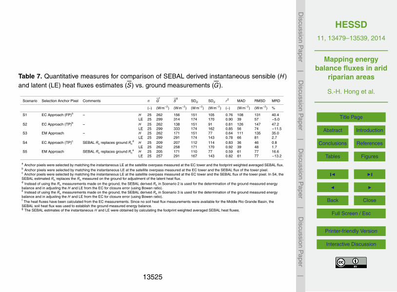
HESSD11, 13479–13539, 2014


riparian areas

S.-H. Hong et al.

Title Page



Tables Figures

J I

J I

Back Close

Full Screen / Esc



Discussion

Paper

|D

iscussionP

aper|

Discussion

Paper

|D

iscussionP

aper|

Table 7. Quantitative measures for comparison of SEBAL derived instantaneous sensible (H)and latent (LE) heat fluxes estimates (S) vs. ground measurements (G).

Scenario Selection Anchor Pixel Comments n Gf

Sg


(–) (Wm−2) (Wm−2) (Wm−2) (Wm−2) (–) (Wm−2) (Wm−2) %

S1 EC Approach (FP)a – H 25 262 156 151 105 0.76 108 131 40.4LE 25 299 314 174 170 0.90 39 57 −5.0

S2 EC Approach (TP)b – H 25 262 138 151 91 0.81 126 147 47.2LE 25 299 333 174 162 0.85 56 74 −11.5

S3 EM Approach – H 25 262 171 151 77 0.64 111 135 35.0LE 25 299 291 174 143 0.78 66 81 2.7

S4 EC Approach (TP)c SEBAL Rn replaces ground Rnd H 25 209 207 112 114 0.83 36 46 0.8

LE 25 262 258 171 170 0.92 39 48 1.7S5 EM Approach SEBAL Rn replaces ground Rn

e H 25 205 171 110 77 0.59 61 77 16.6LE 25 257 291 167 143 0.82 61 77 −13.2

a Anchor pixels were selected by matching the instantaneous LE at the satellite overpass measured at the EC tower and the footprint weighted averaged SEBAL flux.b Anchor pixels were selected by matching the instantaneous LE at the satellite overpass measured at the EC tower and the SEBAL flux of the tower pixel.c Anchor pixels were selected by matching the instantaneous LE at the satellite overpass measured at the EC tower and the SEBAL flux of the tower pixel. In S4, theSEBAL estimated Rn replaces the Rn measured on the ground for adjustment of the latent heat flux.d Instead of using the Rn measurements made on the ground, the SEBAL derived Rn in Scenario 2 is used for the determination of the ground measured energybalance and in adjusting the H and LE from the EC for closure error (using Bowen ratio).e Instead of using the Rn measurements made on the ground, the SEBAL derived Rn in Scenario 3 is used for the determination of the ground measured energybalance and in adjusting the H and LE from the EC for closure error (using Bowen ratio).f The heat fluxes have been calculated from the EC measurements. Since no soil heat flux measurements were available for the Middle Rio Grande Basin, theSEBAL soil heat flux was used to establish the ground measured energy balance.g The SEBAL estimates of the instantaneous H and LE were obtained by calculating the footprint weighted averaged SEBAL heat fluxes.

13525





HESSD11, 13479–13539, 2014


riparian areas

S.-H. Hong et al.

Title Page



Tables Figures

J I

J I

Back Close

Full Screen / Esc



Discussion

Paper

|D

iscussionP

aper|

Discussion

Paper

|D

iscussionP

aper|

Table 8. Quantitative measures for comparison of SEBAL derived daily sensible (H) and latent(LE) heat fluxes estimates (S) vs. ground measurements (G).

EF24 = 1.0×EFinst

Scenario Selection Anchor Pixel n Gf

Sg


(–) MJm−2 day−1 MJm−2 day−1 MJm−2 day−1 MJm−2 day−1 (–) MJm−2 day−1 MJm−2 day−1 %S1 EC Approach (FP)a H 24 6.0 7.2 3.7 3.2 0.41 2.3 3.1 −19.4

LE 24 9.1 8.9 4.4 4.9 0.78 1.7 2.2 2.9S2 EC Approach (TP)b H 24 6.0 6.9 3.7 3.3 0.32 2.6 3.3 −14.9

LE 24 9.1 9.1 4.4 5.0 0.72 2.2 2.6 0.0S3 EM Approach H 24 6.0 7.6 3.7 2.7 0.37 2.6 3.3 −27.0

LE 24 9.1 8.3 4.4 4.2 0.69 1.9 2.6 8.9

EF24 = 1.1×EFinst

Scenario Selection Anchor Pixel n Gf

Sg

SDG SDS r2 MAD RMSD MRD(–) MJm−2 day−1 MJm−2 day−1 MJm−2 day−1 MJm−2 day−1 (–) MJm−2 day−1 MJm−2 day−1 %

S1 EC Approach (FP)a H 24 6.0 6.3 3.7 3.5 0.41 2.1 3.0 −5.6LE 24 9.1 9.7 4.4 5.3 0.78 1.9 2.5 −6.3

S2 EC Approach (TP)b H 24 6.0 6.0 3.7 3.6 0.32 2.7 3.3 −0.8LE 24 9.1 10.0 4.4 5.4 0.71 2.4 3.0 −9.3

S3 EM Approach H 24 6.0 6.9 3.7 3.0 0.42 2.3 2.9 −14.8LE 24 9.1 9.2 4.4 4.6 0.69 2.0 2.5 −0.3

a Anchor pixels were selected by matching the instantaneous LE at the satellite overpass measured at the EC tower and the footprint weighted averaged SEBAL flux.b Anchor pixels were selected by matching the instantaneous LE at the satellite overpass measured at the EC tower and the SEBAL flux of the tower pixel.e Instead of using the Rn measurements made on the ground, the SEBAL derived Rn in Scenario 3 is used for the determination of the ground measured energybalance.f The heat fluxes have been calculated from the EC measurements. Since no soil heat flux measurements were available for the Middle Rio Grande Basin, theSEBAL soil heat flux was used to establish the ground measured energy balance.g The SEBAL estimates of the instantaneous H and LE were obtained by calculating the footprint weighted averaged SEBAL heat fluxes.

13526





HESSD11, 13479–13539, 2014


riparian areas

S.-H. Hong et al.

Title Page



Tables Figures

J I

J I

Back Close

Full Screen / Esc



Discussion

Paper

|D

iscussionP

aper|

Discussion

Paper

|D

iscussionP

aper|

1099 1100 1101

1102 1103 1104

1105 1106 1107 1108

1109

1110

1111

1112

Figure 1. Distribution of energy balance relative closure (H+LE)/(Rn–G) of instantaneous 1113

(top panel) and total daily (bottom panel) fluxes from eddy covariance towers. Each ‘bar’ 1114

represents a satellite overpass day. The dotted lines show criteria of acceptable closure 1115

[65 and 110 %] and percentage of the data having acceptable closure is shown in bracket. 1116

1117

50

Figure 1. Distribution of energy balance relative closure (H+LE)/(Rn−G) of instantaneous (toppanel) and total daily (bottom panel) fluxes from eddy covariance towers. Each “bar” representsa satellite overpass day. The dotted lines show criteria of acceptable closure (65 and 110 %)and percentage of the data having acceptable closure is shown in bracket.

13527





HESSD11, 13479–13539, 2014


riparian areas

S.-H. Hong et al.

Title Page



Tables Figures

J I

J I

Back Close

Full Screen / Esc



Discussion

Paper

|D

iscussionP

aper|

Discussion

Paper

|D

iscussionP

aper|

1118

1119

1120

1121

1122

1123

1124 1125 1126

1127 1128 1129 1130 1131 1132 1133 1134 1135 1136 1137

1138

1139

Figure 2. Footprint size and footprint intensity from the eddy covariance tower located at 1140

SEV (saltcedar) in Rio Grande on August 19, 2002 (10:40 am) (wind speed: 3.4 m/s, 1141

vegetation height: 4.9 m and sonic anemometer height from ground: 6.5 m). 1142

1143

51

Figure 2. Footprint size and footprint intensity from the eddy covariance tower located at SEV(saltcedar) in Rio Grande on 19 August 2002 (10:40 a.m.) (wind speed: 3.4 ms−1, vegetationheight: 4.9 m and sonic anemometer height from ground: 6.5 m).

13528





HESSD11, 13479–13539, 2014


riparian areas

S.-H. Hong et al.

Title Page



Tables Figures

J I

J I

Back Close

Full Screen / Esc



Discussion

Paper

|D

iscussionP

aper|

Discussion

Paper

|D

iscussionP

aper|

Figure 3. SEBAL daily evapotranspiration (mmday−1) maps along the Rio Grande in spring,summer and fall.

13529





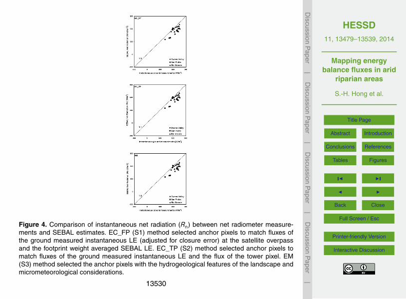
HESSD11, 13479–13539, 2014


riparian areas

S.-H. Hong et al.

Title Page



Tables Figures

J I

J I

Back Close

Full Screen / Esc



Discussion

Paper

|D

iscussionP

aper|

Discussion

Paper

|D

iscussionP

aper|

1161

1162 1163 1164

1165 1166 1167

1168 1169

1170

1171

Figure 4. Comparison of instantaneous net radiation (Rn) between net radiometer 1172

measurements and SEBAL estimates. (EC_FP (S1) method selected anchor pixels to 1173

match fluxes of the ground measured instantaneous LE (adjusted for closure error) at the 1174

satellite overpass and the footprint weight averaged SEBAL LE. EC_TP (S2) method 1175

selected anchor pixels to match fluxes of the ground measured instantaneous LE and the 1176

flux of the tower pixel. EM (S3) method selected the anchor pixels with the 1177

hydrogeological features of the landscape and micrometeorological considerations. 1178

1179

53

Figure 4. Comparison of instantaneous net radiation (Rn) between net radiometer measure-ments and SEBAL estimates. EC_FP (S1) method selected anchor pixels to match fluxes ofthe ground measured instantaneous LE (adjusted for closure error) at the satellite overpassand the footprint weight averaged SEBAL LE. EC_TP (S2) method selected anchor pixels tomatch fluxes of the ground measured instantaneous LE and the flux of the tower pixel. EM(S3) method selected the anchor pixels with the hydrogeological features of the landscape andmicrometeorological considerations.

13530





HESSD11, 13479–13539, 2014


riparian areas

S.-H. Hong et al.

Title Page



Tables Figures

J I

J I

Back Close

Full Screen / Esc



Discussion

Paper

|D

iscussionP

aper|

Discussion

Paper

|D

iscussionP

aper|

1180

1181

1182

1183

1184

1185

1186

1187

1188

1189

1190

1191

1192 1193

1194

1195

1196

1197

1198

1199

1200

1201

1202

1203

1204

1205

1206

1207

1208

1209

Figure 5. Comparison of daily net radiation (Rn) between net radiometer measurements 1210

and SEBAL estimates. 1211

1212

54

Figure 5. Comparison of daily net radiation (Rn) between net radiometer measurements andSEBAL estimates.

13531





HESSD11, 13479–13539, 2014


riparian areas

S.-H. Hong et al.

Title Page



Tables Figures

J I

J I

Back Close

Full Screen / Esc



Discussion

Paper

|D

iscussionP

aper|

Discussion

Paper

|D

iscussionP

aper|

1213

1214

1215 1216 1217

1218 1219 1220

1221 1222 1223 1224

1225

1226

1227

1228

Figure 6. Comparison of instantaneous ground heat flux (G) between soil heat flux plate 1229

measurements and SEBAL estimates in Owens Valley and San Pedro Valley. 1230

1231

55

Figure 6. Comparison of instantaneous ground heat flux (G) between soil heat flux plate mea-surements and SEBAL estimates in Owens Valley and San Pedro Valley.

13532





HESSD11, 13479–13539, 2014


riparian areas

S.-H. Hong et al.

Title Page



Tables Figures

J I

J I

Back Close

Full Screen / Esc



Discussion

Paper

|D

iscussionP

aper|

Discussion

Paper

|D

iscussionP

aper|

Figure 7. Comparison of sensible (H) and latent heat (LE) fluxes between adjusted eddy co-variance tower measurements and SEBAL estimates from scenario S2 (EC_TP).

13533





HESSD11, 13479–13539, 2014


riparian areas

S.-H. Hong et al.

Title Page



Tables Figures

J I

J I

Back Close

Full Screen / Esc



Discussion

Paper

|D

iscussionP

aper|

Discussion

Paper

|D

iscussionP

aper|

1262

1263

1264

1265

1266

1267

1268

1269 1270

1271

1272 1273

1274

1275

1276

1277

1278

1279

1280

1281

1282

1283

1284

1285

1286

Figure 8. Comparison of instantaneous sensible heat flux (H) between adjusted eddy 1287

covariance tower measurements and SEBAL estimates for scenarios S1–S5. 1288

57

Figure 8. Comparison of instantaneous sensible heat flux (H) between adjusted eddy covari-ance tower measurements and SEBAL estimates for scenarios S1–S5.

13534





HESSD11, 13479–13539, 2014


riparian areas

S.-H. Hong et al.

Title Page



Tables Figures

J I

J I

Back Close

Full Screen / Esc



Discussion

Paper

|D

iscussionP

aper|

Discussion

Paper

|D

iscussionP

aper|

1289

1290

1291

1292

1293

1294

1295

1296 1297

1298

1299

1300 1301

1302

1303

1304

1305

1306

1307

1308

1309

1310

1311

1312

1313

Figure 9. Comparison of instantaneous latent heat flux (LE) between adjusted eddy 1314

covariance tower measurements and SEBAL estimates for scenarios S1–S5. 1315

58

Figure 9. Comparison of instantaneous latent heat flux (LE) between adjusted eddy covariancetower measurements and SEBAL estimates for scenarios S1–S5.

13535





HESSD11, 13479–13539, 2014


riparian areas

S.-H. Hong et al.

Title Page



Tables Figures

J I

J I

Back Close

Full Screen / Esc



Discussion

Paper

|D

iscussionP

aper|

Discussion

Paper

|D

iscussionP

aper|

1316

1317

1318

1319

1320

1321

1322

1323 1324

1325

1326

1327

1328

1329

1330

1331

1332

1333

1334

1335

1336

1337

1338

1339

1340

1341

Figure 10. Comparison of satellite overpass instantaneous evaporative fraction (EF) with 1342

daytime average measured on the ground. 1343

1344

59

Figure 10. Comparison of satellite overpass instantaneous evaporative fraction (EF) with day-time average measured on the ground.

13536





HESSD11, 13479–13539, 2014


riparian areas

S.-H. Hong et al.

Title Page



Tables Figures

J I

J I

Back Close

Full Screen / Esc



Discussion

Paper

|D

iscussionP

aper|

Discussion

Paper

|D

iscussionP

aper|

1345

1346

1347

1348

1349

1350

1351

1352

1353

1354 1355

1356

1357

1358

1359

1360

1361

1362

1363

1364

1365

1366

1367

1368

1369

1370

1371

1372

1373

1374

1375

1376

1377

Figure 11. Comparison of daily sensible heat flux (H) between adjusted eddy covariance 1378

tower measurements and SEBAL estimates. (EF24 = 1.1* EFinst) 1379

1380

60

Figure 11. Comparison of daily sensible heat flux (H) between adjusted eddy covariance towermeasurements and SEBAL estimates (EF24 = 1.1×EFinst).

13537





HESSD11, 13479–13539, 2014


riparian areas

S.-H. Hong et al.

Title Page



Tables Figures

J I

J I

Back Close

Full Screen / Esc



Discussion

Paper

|D

iscussionP

aper|

Discussion

Paper

|D

iscussionP

aper|

1381 1382 1383 1384 1385 1386 1387 1388 1389 1390 1391 1392

1393 1394 1395 1396

1397

1398

1399

1400

1401

1402

1403

1404

1405

1406

1407

1408

1409

1410

1411

1412

1413

1414

1415

Figure 12. Comparison of daily latent heat flux (LE) between adjusted eddy covariance 1416

tower measurements and SEBAL estimates. (EF24 = 1.1* EFinst) 1417

1418

61

Figure 12. Comparison of daily latent heat flux (LE) between adjusted eddy covariance towermeasurements and SEBAL estimates (EF24 = 1.1×EFinst).

13538





HESSD11, 13479–13539, 2014


riparian areas

S.-H. Hong et al.

Title Page



Tables Figures

J I

J I

Back Close

Full Screen / Esc



Discussion

Paper

|D

iscussionP

aper|

Discussion

Paper

|D

iscussionP

aper|

1419

1420

1421

1422

1423

1424

1425

1426

1427

1428

1429

1430 1431

1432

1433

1434

1435

1436

1437

1438

1439

1440

1441

1442

1443

1444

1445

1446

1447

1448

1449

1450

Figure 13. Comparison of ET rates determined from SEBAL with cEF of 1.1 to eddy 1451

covariance ground measurements in riparian areas of the Rio Grande Valley (NM), San 1452

Pedro Valley (AZ), and Owens Valley (CA). 1453

1454

62

Figure 13. Comparison of ET rates determined from SEBAL with cEF of 1.1 to eddy covarianceground measurements in riparian areas of the Rio Grande Valley (NM), San Pedro Valley (AZ),and Owens Valley (CA).

13539





Evaluation of an extreme-condition-inverse calibration remote

Documents

Transcript of Evaluation of an extreme-condition-inverse calibration remote