Evaluation and Performance Enhancement of Cooling Tower ...

Evaluation and Performance Enhancement of

Cooling Tower Spray Patterns

Thesis presented in fulfilment of the requirements for the degree

Master of Engineering (Mechanical)


Cooling Tower Spray Patterns

by

Daniël Roux

December 2012

presented in fulfilment of the requirements for the degree

of Engineering (Mechanical) in the Faculty of Engineering

Stellenbosch University

Supervisor: Prof. Hanno Carl Rudolf Reuter


presented in fulfilment of the requirements for the degree of

Engineering at

i

DECLARATION

By submitting this thesis electronically, I declare that the entirety of the work contained therein is my own, original work, that I am the sole author thereof (save to the extent explicitly otherwise stated), that reproduction and publication thereof by Stellenbosch University will not infringe any third party rights and that I have not previously in its entirety or in part submitted it for obtaining any qualification. Signature:...................................... Date:.............................................. Copyright © 2012 Stellenbosch University All rights reserved

Stellenbosch University http://scholar.sun.ac.za

ii

ABSTRACT

The performance of wet cooling towers can be improved by installing spray nozzles that distribute the cooling water uniformly onto the fill whilst operating at a low pressure head. In this thesis, three commercial spray nozzles are experimentally evaluated in terms of flow and pressure loss characteristics as well as water distribution patterns. The results of the evaluation process highlight the need for spray nozzles with enhanced performance characteristics. The theory required to implement the results of the evaluation process in the design of a cooling tower is presented and discussed. A systematic approach to enhance the performance of a spray nozzle through minor alterations is applied to one of the commercial spray nozzles that was evaluated. The fluid dynamics of an orifice nozzle, such as the effect of a change in pressure head, spray angle, spray height, orifice diameter and wall thickness on drop diameter and spray distance, is experimentally investigated and a model with which a spray nozzle can be designed is finally presented. Two prototype spray nozzles show that it is possible to enhance the performance of spray nozzles and thus wet cooling towers by means of the methods presented.


iii

SAMEVATTING

Die werkverrigting van natkoeltorings kan verbeter word deur sproeiers te installeer wat die verkoelingswater uniform versprei op die pakking teen 'n lae pomp drukhoogte. In hierdie tesis word drie kommersiële sproeiers eksperimenteel geëvalueer in terme van vloei en drukverlies eienskappe sowel as water verdelings patrone. Die resultate van die evaluasie proses beklemtoon die behoefte aan sproeiers met verbeterde werkverrigtingseienskappe. Die teorie wat benodig word om die resultate van die evaluasie proses te implementeer in die ontwerp van 'n natkoeltoring word bespreek. 'n Stelselmatige benadering om die werkverrigtings van 'n sproeier te verhoog deur klein veranderinge aan die ontwerp aan te bring, word toegepas op een van die sproeiers wat getoets is. Die vloeidinamika van 'n plaatmondstuk, soos die effek van 'n verandering in drukhoogte, sproeihoek, sproeihoogte, gatdiameter en wanddikte op druppel diameter en sproeiafstand, is eksperimenteel ondersoek en 'n model word aangebied waarmee 'n sproeier ontwerp kan word. Twee prototipe sproeiers wys dat dit moontlik is om die werkverrigting van sproeiers, en dus ook natkoeltorings, te verbeter deur die metodes wat in die tesis aangebied word, toe te pas.


iv

ACKNOWLEDGEMENTS

I would like to thank the following people who aided me throughout this project: My parents who throughout my life provided me with their love and support and for giving me the best opportunities any child could ask for. My girlfriend, Liezl, for her love, laughter and support. Thank you for always listening and expressing your interest in my work. My supervisor, Prof Reuter, for sharing your knowledge throughout all our conversations, the expert guidance and friendly encouragement. Mr. Cobus Zietsman for all the help. Ferdi, Calvin, Graham, Anton and all the workshop personnel for the manufacturing and advice. Juliun Stanfliet for all the help and conversations.


v

TABLE OF CONTENTS

List of figures ........................................................................................................ vii

List of tables ............................................................................................................. x

Nomenclature .......................................................................................................... xi

1 Introduction ...................................................................................................... 1

1.1 Background ................................................................................. 1

1.2 Objectives ................................................................................... 3

1.3 Motivation .................................................................................. 3

1.4 Literature review ........................................................................ 3

2 Spray Nozzle Performance Evaluation ............................................................ 6

2.1 Introduction ................................................................................ 6

2.2 Theory ......................................................................................... 6

2.2.1 Flow rate ............................................................................................ 6

2.2.2 Pipe friction losses ............................................................................. 7

2.2.3 Nozzle inlet total pressure head ......................................................... 7

2.2.4 Loss coefficient through a nozzle ...................................................... 8

2.2.5 Loss coefficient across a nozzle ......................................................... 9

2.2.6 Water distribution ............................................................................ 10

2.3 Experimental facility ................................................................ 10

2.3.1 Description of experimental apparatus ............................................ 10

2.3.2 Measurement techniques .................................................................. 12

2.3.3 Test procedure .................................................................................. 14

2.4 Description of test nozzles ........................................................ 15

2.5 Results ...................................................................................... 16

2.5.1 Flow characteristics ......................................................................... 16

2.5.2 Loss coefficients .............................................................................. 26


2.6 Summary and conclusions ........................................................ 36

3 Implementation and Application of Spray Nozzle Performance Characteristics ........................................................................................................ 37

3.1 Introduction .............................................................................. 37

3.2 Implementation and application ............................................... 37

3.2.1 Flow characteristics and loss coefficients ........................................ 37


vi



4 Spray Nozzle Performance Enhancement ...................................................... 42

4.1 Introduction .............................................................................. 42

4.2 Description of the test nozzle ................................................... 42

4.3 Results ...................................................................................... 43


5 Spray Nozzle Design ..................................................................................... 50

5.1 Introduction .............................................................................. 50

5.2 Theory ....................................................................................... 51

5.2.1 Single drop trajectory model ............................................................ 51

5.2.2 Derived design equations ................................................................. 56

5.3 Experimental facility ................................................................ 56

5.3.1 Description of experimental apparatus ............................................ 56

5.3.2 Measurement techniques .................................................................. 57

5.3.3 Test procedure .................................................................................. 59

5.4 Orifice nozzle test results ......................................................... 59

5.4.1 Drop diameter .................................................................................. 59

5.4.2 Spray range deviation ...................................................................... 61

5.4.3 Spray scatter ..................................................................................... 63

5.4.4 Bypass flow ...................................................................................... 66

5.5 Spray nozzle designs ................................................................ 67

5.5.1 Design .............................................................................................. 67

5.5.2 Water distribution patterns ............................................................... 71

5.5.3 Comparative evaluation ................................................................... 74


6 Summary and conclusions ............................................................................. 77

References .............................................................................................................. 79

Appendices ............................................................................................................. 81

Appendix A Calibration data ........................................................................ 81

Appendix B Sample calculations .................................................................. 83


vii

LIST OF FIGURES

Figure 1.1: Schematic layout of a natural draft wet cooling tower .......................... 2

Figure 1.2: Effect of water maldistribution on tower performance (Kranc, 1993) ........................................................................................................................ 4

Figure 2.1: Schematic layout of piezometers for pipe friction ................................ 7

Figure 2.2: Schematic layout of piezometer for the nozzle inlet static pressure measurements ........................................................................................................... 8

Figure 2.3: Schematic layout of piezometer for the measurement of the loss across a nozzle .................................................................................................................... 9

Figure 2.4: Experimental apparatus ....................................................................... 12

Figure 2.5: Piezometer ........................................................................................... 13

Figure 2.6: Pipe friction verification ...................................................................... 13

Figure 2.7: Compartmentalised measurement trough ............................................ 14

Figure 2.8: Shutter system with buckets used for simultaneous flow measurement 14

Figure 2.9: Schematic presentation of the test nozzles .......................................... 16

Figure 2.10: Flow characteristics for nozzle no. 1 and 2 ....................................... 17

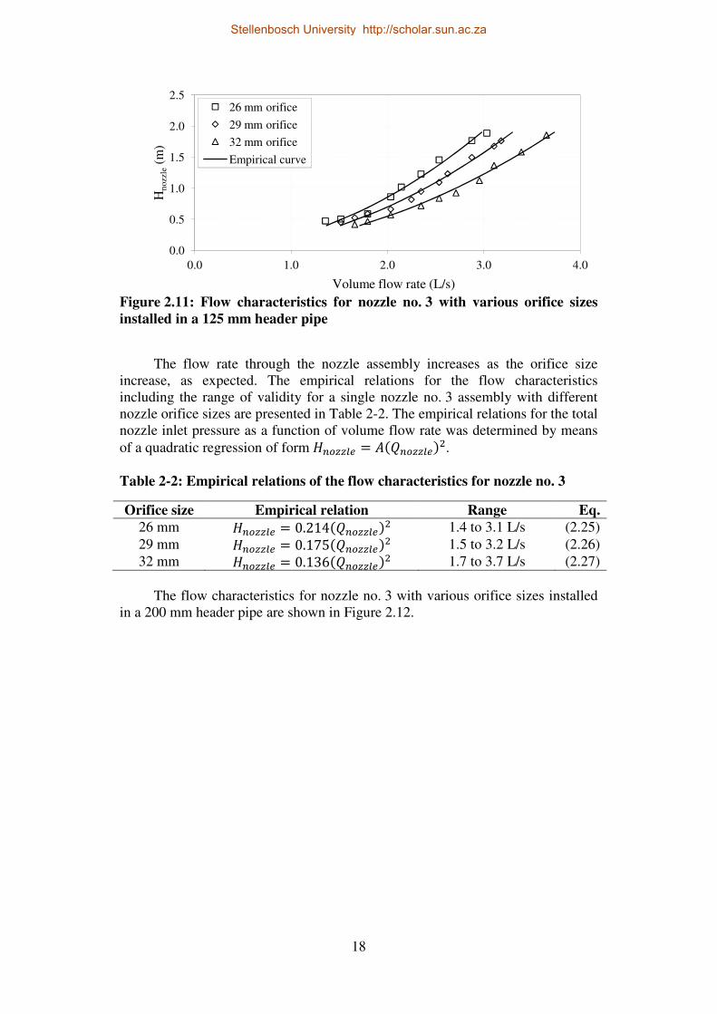
Figure 2.11: Flow characteristics for nozzle no. 3 with various orifice sizes installed in a 125 mm header pipe ......................................................................... 18

Figure 2.12: Flow characteristics for nozzle no. 3 with various orifice sizes installed in a 200 mm header pipe ......................................................................... 19

Figure 2.13: Flow characteristics for three nozzle no. 3 assemblies with various orifice sizes ............................................................................................................ 20

Figure 2.14: Flow characteristics for nozzle no. 3 with various orifice sizes and bypass flow ............................................................................................................ 21

Figure 2.15: Effect of bypass flow on the flow characteristics for a single nozzle no. 3 assembly with various orifice sizes .............................................................. 23

Figure 2.16: Flow characteristics for three nozzle no. 3 assemblies with various orifice sizes and bypass flow ................................................................................. 24

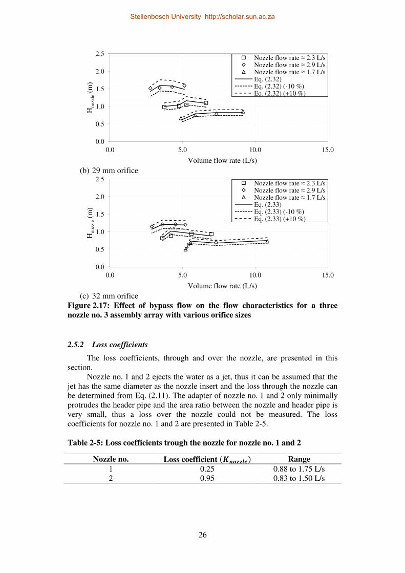
Figure 2.17: Effect of bypass flow on the flow characteristics for a three nozzle no. 3 assembly array with various orifice sizes ..................................................... 26

Figure 2.18: Pipe friction losses for a single nozzle assembly with no flow through the nozzles .............................................................................................................. 27

Figure 2.19: Pipe friction losses for three nozzle no. 3 assemblies with no flow through the nozzles ................................................................................................ 28

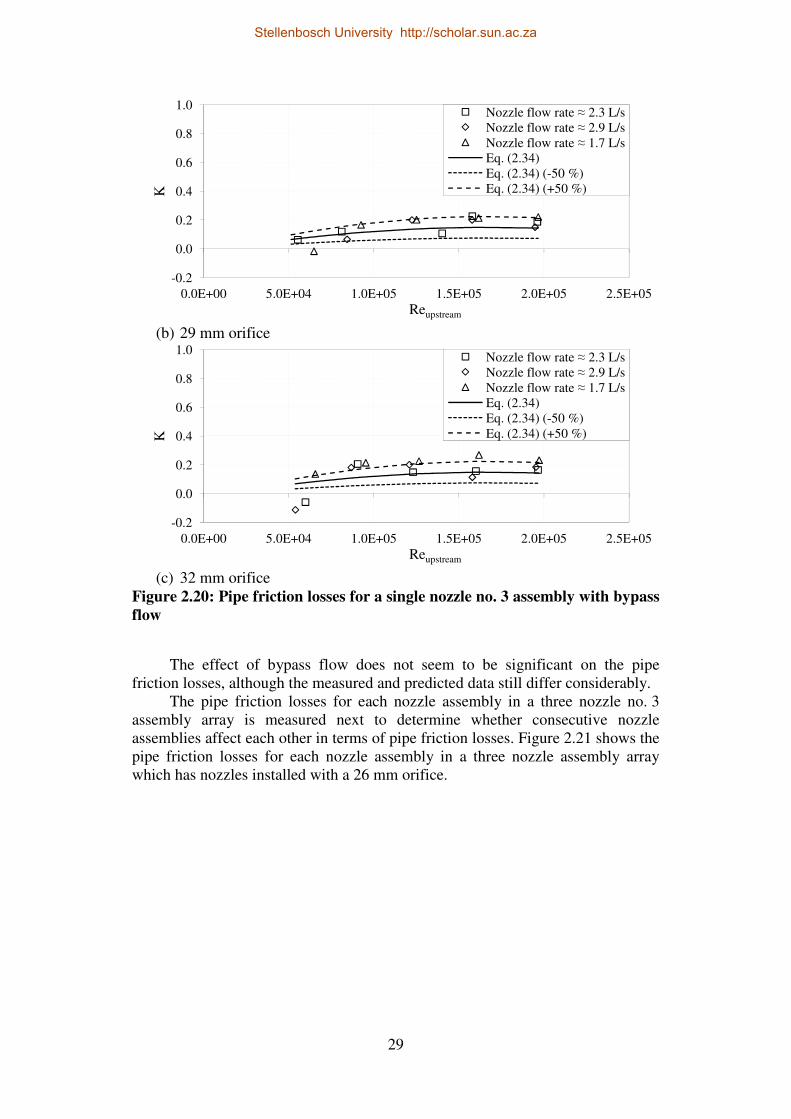
Figure 2.20: Pipe friction losses for a single nozzle no. 3 assembly with bypass flow 29


viii

Figure 2.21: Pipe friction losses for three nozzle assemblies with bypass flow for nozzles with a 26 mm orifice ................................................................................. 30



Figure 2.24: Water distribution pattern for nozzle no. 1 ....................................... 33

Figure 2.25: Water distribution pattern for nozzle no. 2 ....................................... 34

Figure 2.26: Water distribution patterns for a single nozzle no. 3 assembly with different nozzle orifice sizes .................................................................................. 35

Figure 3.1: Comparison between the superimposed and measured water distribution patterns for two nozzle no. 3 assemblies with different nozzle orifice sizes 40

Figure 4.1: Initial test results for the original nozzle ............................................. 44

Figure 4.2: Test results for the modified nozzle .................................................... 47

Figure 5.1: Schematic layout of the experimental investigation ........................... 51

Figure 5.2: Schematic layout of the forces and velocities acting in on the drop ... 52

Figure 5.3: Trajectory of a 2 mm drop sprayed from an initial angle of 30° with a 0.5 m pressure head ............................................................................................... 54

Figure 5.4: Effect of various parameters on the spray range ................................. 55

Figure 5.5: Orifice nozzle experimental apparatus ................................................ 57

Figure 5.6: Photographed drops ............................................................................. 58

Figure 5.7: Test results for the drop diameters produced by an orifice nozzle ...... 60

Figure 5.8: Tapered orifices directions .................................................................. 61

Figure 5.9: Test results for the spray range deviation ............................................ 62

Figure 5.10: Spray range deviation for a tapered hole ........................................... 63

Figure 5.11: Spray scatter produced by a tapered 1 mm orifice with a spray angle of 0° at various pressure heads and spray heights ................................................. 64

Figure 5.12: Spray scatter produced by a tapered 1 mm orifice with a pressure head of 0.45 m at various spray angles and spray heights ..................................... 65

Figure 5.13: Spray scatter produced by a tapered 2 mm orifice with a spray height of 0.5 m .................................................................................................................. 65

Figure 5.14: Relationship of the y – direction velocity component and the pipe velocity for a 2.15 mm tapered hole ...................................................................... 66

Figure 5.15: Relationship of the y – direction velocity component and the pipe velocity for various hole diameters ........................................................................ 67

Figure 5.16: Schematic of a pipe and sphere spray nozzle .................................... 68


ix

Figure 5.17: Pipe spray nozzle in operation .......................................................... 69

Figure 5.18: Sphere spray nozzle in operation ...................................................... 70

Figure 5.19: Design procedure ............................................................................... 70

Figure 5.20: Pipe spray nozzle water distribution pattern ..................................... 71

Figure 5.21: Measured and predicted water distribution patterns for a single row of orifice nozzles .................................................................................................... 72

Figure 5.22: Laser cut pipe spray nozzle water distribution pattern ...................... 72

Figure 5.23: Sphere spray nozzle water distribution pattern ................................. 73

Figure 5.24: Possible installation configurations of the spray nozzle designs ...... 75

Figure A.1: Venturi flow meter and calibration curve ........................................... 81

Figure A.2: Drop size calibration photo ................................................................ 82


x

LIST OF TABLES

Table 2-1: Empirical relations of the flow characteristics for nozzle no. 1 and 2. 17

Table 2-2: Empirical relations of the flow characteristics for nozzle no. 3. .......... 18

Table 2-3: Empirical relations of the flow characteristics with bypass flow for nozzle no. 3. ........................................................................................................... 22

Table 2-4: Empirical relations of the flow characteristics with bypass flow for the second nozzle assembly in a three nozzle no. 3 assembly array. ........................... 25

Table 2-5: Loss coefficients trough the nozzle for nozzle no. 1 and 2. ................. 26

Table 2-6: Empirical relation of the pipe friction loss coefficient for a single nozzle no. 3 assembly with no flow through the nozzles. ..................................... 27

Table 2-7: Christiansen coefficient for nozzle no. 3 with different nozzle orifice sizes. ....................................................................................................................... 35

Table 3-1: Comparison between the superimposed and measured Christiansen coefficients. ............................................................................................................ 40

Table 4-1: Initial performance parameters for the original nozzle. ....................... 44

Table 4-2: Summary of results. .............................................................................. 47

Table 4-3: Performance parameters for the modified nozzle. ............................... 49

Table 5-1: Test results for the drop diameters produce by a tapered orifice nozzle. ............................................................................................................................... 61

Table 5-2: Water distribution pattern test results. .................................................. 74

Table B‒1: Sample calculation data for the flow characteristics of nozzle no. 1. . 83

Table B‒2: Sample calculation data for the loss coefficient through nozzle no. 1. ............................................................................................................................... 84

Table B‒3: Sample calculation data for the loss coefficient across nozzle no. 3 assembly with 26 mm orifice diameter nozzles. .................................................... 85

Table B‒4: Sample calculation data for the water distribution of nozzle no. 1. .... 86

Table B‒5: Sample calculation data for the single drop trajectory model. ............ 87


xi

NOMENCLATURE

A Area, m2

C Discharge or contraction coefficient Cu Christiansen coefficient d Diameter, m e Energy, J F Force, N f Darcy friction factor G Mass flux, kg/m2s ∆G Mass flux deviation Ḡ Average mass flux, kg/m2s g Gravitational acceleration, m/s2 H Total head, m h Height reading, m ∆h Height difference reading, m K Loss coefficient L Length, m M Mass, kg m Mass flow rate, kg/s n Number of measurement points or orifices p Pressure, Pa Q Volume flow rate, L/s Re Reynolds number S Spacing, m ∆t Time, s tw Wall thickness, m V Volume, L v Velocity, m/s x Co-ordinate, m y Co-ordinate, m z Co-ordinate or height, m

Greek symbols

αe Kinematic energy coefficient β Contraction ratio ε Roughness height, mm ϵ Efficiency θ Angle, ° µ Kinematic viscosity, m2/s ρ Density, kg/m3

Φ Angle, °


xii

Subscripts a Air ad Air-drop atm Atmosphere B Buoyancy bypass Bypass bypass tank Bypass tank c Compartment D Drag d Drop G Gravity Global Global Hg Mercury / Mercury manometer in In Local Local nozzle Nozzle nozzle bucket Nozzle bucket max Maximum mechanical Mechanical or Orifice p Piezometer photograph Photograph pixel Pixel pipe Pipe or pipe spray nozzle projected Projected sphere Sphere spray nozzle spray Spray T Total vi Venturi inlet vt Venturi throat w Water x x-direction y y-direction z z-direction

Superscripts

t Time step

Abbreviations

HVAC Heating, ventilation and air conditioning NP Nozzle pitch VSD Variable speed drive


1

1 INTRODUCTION

1.1 Background

A spray nozzle is a device used to convert a liquid into a spray to facilitate mainly wetting of a given surface area, cooling of the liquid and/ or dispersion of the liquid into a gas stream e.g. for combustion or de-aeration processes. Uniform wetting requires the liquid to be distributed evenly over a specific area and maximum cooling requires the surface area of the liquid to be increased by reducing the mean drop size as well as an even drop dispersion. Spray nozzles are used in various applications in modern industry. These include HVAC systems for building cooling and air conditioning, fire protection, petrochemical and combustion for spraying petroleum, power generation for rejecting excess process heat and in agricultural applications for irrigation.

This thesis focuses on spray nozzles used in wet cooling towers which are used to reject excess process heat to the atmosphere through evaporative cooling, where water comes into direct contact with atmospheric air. Wet cooling towers are classified as natural draft or mechanical draft. Natural draft cooling towers operate on a buoyancy effect where the density difference between the air inside and outside of the structure causes a draft through the cooling tower. Mechanical draft cooling towers rely on fans to force air through the structure in order to create a forced draft or air is sucked through the structure to create an induced draft. The structures of mechanical draft cooling towers are much smaller than those of natural draft cooling towers, but their life cycle costs are higher for large systems mainly due to the power consumption of the fans. Fan assisted natural draft cooling towers are a combination of the two, where fans are installed at the base of the hyperbolic structure to create a combined forced-natural draft. Thus the overall height of the structure is reduced and less power is required to drive the fans.

Figure 1.1 shows a schematic layout of a natural draft wet-cooling tower. The spray nozzles can be seen as the first stage of the cooling process occurring in the cooling tower. Heated process cooling water from the plant is distributed onto a fill material by means of the spray nozzles, which are installed in distribution header pipes. The water runs through the fill material and drips down into the catchment pond where it is collected. From the catchment pond it is pumped back to the plant.


2

Figure 1.1: Schematic layout of a natural draft wet cooling tower

The spray zone is a critical part of the cooling process since it contributes to

the overall cooling but also affects the performance of the fill material directly. Defining and improving the nozzle performance characteristics will lead to higher cooling capacities and overall plant efficiencies. Water spray nozzle performance characteristics include water distribution, required pressure head and drop size distribution. Uniform water distribution is desirable in a spray nozzle design to ensure the effective usage of the whole fill material area as opposed to uneven distribution with high water concentrations at localised areas and less or no water in other areas. Low pressure heads are also desirable and thus the pressure drop over the nozzle should be minimal. This would ensure that lower pump energy is required and thus lower operating cost. Drop sizes should be small in order to maximise the heat transfer but should also not be too small to prevent the drops from being blown out of the cooling tower structure which will lead to additional water loss, higher running costs and contamination of ground water.

New nozzle designs and improvement of current designs have not received much attention and very limited information can be found regarding this topic in literature. This project will focus on the evaluation and performance enhancement of current nozzle designs as well as the development and testing of a new nozzle design.

Drift eliminator

Spray nozzle

Spray zone

Fill material

Rain zone

Catchment pond

Water in

Water Out

Air in

Air out


3

1.2 Objectives

The following objectives are set out in order to evaluate and improve the performance of cooling tower spray zones:

• Evaluate the performance of various commercially available spray nozzles in terms of flow characteristics and water distribution.

• Evaluate the effect on the performance characteristics of an array of spray nozzles relative to a single nozzle.

• Improve the performance of such a spray nozzle based on the performance evaluation results.

• Determine the drop size and water distribution for a water jet ejected from an orifice nozzle.

• Design and test two new spray nozzles which implements numerous orifice nozzles to deliver a predictable water distribution.

1.3 Motivation

In recent years power demand has drastically increased which has put the environment under severe strain. The power output of a power plant can be increased by increasing the cooling capacity of the cooling system. This can be achieved by enhancing the performance of the spray zone in a wet cooling tower by means of improved spray nozzle designs offering a cost effective way to improve the performance of new and currently operating cooling towers and power plants.

This project will improve the understanding of cooling tower spray nozzle designs in general. It presents and discusses methods by which the performance characteristics of spray nozzles can be determined and implemented to optimise new and current cooling tower layouts, which will ultimately lead to improved performance, lowered operating costs and environmental impacts.

1.4 Literature review

Tognotti et al. (1991) stated that the water distribution on the fill of a cooling tower is a key aspect for the performance of the overall cooling system. An experimental study was conducted on the water distribution of a pilot cooling tower. Various industrial spray nozzles were investigated. The nozzles were evaluated based on various performance parameters such as the Sauter mean drop diameter, the ratio between the wetted area at a specific distance from the nozzle to the whole area under the nozzle and the uniformity of the water distribution expressed in terms of the standard deviation between measured data. The results showed that a correlation exist between the nozzle performance in single nozzle installation and in arrangements of nozzle installations. The uniformity of the


4

water distribution was found to be strongly related to the installation pattern and the operating conditions. It was also found that coalescence plays an important role on the drop size distribution in the pilot-tower.

The interrelated design problems regarding the hydraulic performance of a nozzle array and the influence of water deposition on the overall thermal performance was investigated by Kranc (1993a). The tower performance in terms of a cooling range ratio was determined as a function of work input, the pumping power and the uniformity of the water distribution, as expressed by the Christiansen coefficient. The effects of overlapping and interaction between adjacent nozzles were investigated by means of superpositioning of single nozzle data. The results showed that the performance could be increased by intelligent designing such as selecting correct internal components and configurations. It was also found that the fill configuration may not easily be changed and cannot sufficiently correct poor water distribution.

A further study conducted by Kranc (1993b) presented a model which quantified the effect of water maldistribution on the tower performance. Figure 1.2 shows the decrease in tower performance as the uniformity of the water distribution decreases for different fill configurations and nozzle spray patterns as indicated by the various markers. The tower performance is defined as the actual to ideal cooling range ratio and the uniformity of the water distribution is expressed in terms of the Christiansen coefficient. The Christiansen coefficient provides a quantitative measure of the deviation between all of the mass flux measurements below a nozzle, and is often used to characterise irrigation. This indicates that if the water distribution of a particular spray nozzle has a Christiansen coefficient of 0.50 then the actual cooling range would be 86 % of the ideal range. Thus to achieve the required cooling the water flow rate has to be increased by approximately 13 % which results in higher auxiliary power consumption and water consumption. This leads to an increase in operating costs and environmental impacts.

Figure 1.2: Effect of water maldistribution on tower performance

(Kranc, 1993)


5

Kranc (2006) investigated the optimal spray patterns for two generic spray nozzles, one that delivers a circular spray pattern and one that delivers an annular spray pattern. The optimum spacing of these nozzles when installed in a square array was determined to deliver the most uniform distribution. It was found that the nozzle with the highest thermal performance properties only performed slightly better than the nozzle with the highest uniformity. It is stated that the uniformity of the water distribution delivered by a nozzle is an adequate consideration when selecting a nozzle.

Xiaoni et al. (2006) developed a one-dimensional model to study the trajectory and the evaporative cooling process at water drop level. This model was based on a kinematic model and a heat transfer model. It provided a theoretical foundation for practical applications in the cooling tower industry and nozzle designing.

Viljoen (2006) tested two low pressure nozzles and superimposed the data obtained to predict the water distribution for an arrangement of four nozzles. The four nozzle arrangement was also tested and it was found that it is possible to predict the water distribution of arrangements of nozzles using superposition. A set of ideal spray nozzle characteristics was formed in terms of the nozzle design, spray drops and the water distribution. The performance criteria were used to evaluate real nozzle characteristics and it was found that the nozzle performance is lacking and that improvements are required to reach the ideal characteristics.

Vitkovic and Syrovatka (2009) also tested a low pressure nozzle and the corresponding nozzle array spacing was determined by means of superpositioning of the test data. The nozzle spacing to ensure optimal water distribution was obtained through Simplex method optimisation techniques.

Reuter et al. (2010a) presented a method by which the performance characteristics of a cooling tower spray zone could be determined. The water distribution, inlet pressure and drop size data of a nozzle was experimentally determined, where after this data was used to determine the performance characteristics of the spray zone produced by a grid of the nozzles in terms of the Merkel number and loss coefficient. A single drop trajectory and heat transfer model was used as well as CFD analysis.

The literature mentioned above provides this project with a well established foundation to work from. A few theoretical models have been developed for the predicting of the performance characteristics of cooling towers. However, no literature was found on spray nozzle designs that deliver near uniform water distributions. Thus further investigation in new and current nozzle designs is very important.


6

2 SPRAY NOZZLE PERFORMANCE EVALUATION

2.1 Introduction

The performance of a spray nozzle can be evaluated based on various design aspects and parameters. According to Viljoen (2006) the ideal nozzle design should be robust in terms of chemical, abrasion and clogging resistance as well as easily installed and maintained in a cooling tower environment. It should be invertible for up and down spray applications and should not affect the airflow over it, thus having a low air pressure drop over the nozzle. Drops should ideally form immediately, without sheet or ligament formation, and should have a uniform diameter as well as mass fraction. The drops should be large enough to ensure that it is not blown out of the tower structure, ideally 1 to 2 mm in diameter. The air contact time should be identical and as long as possible for all the drops and there should be no collision between drops or distribution pipes to prevent seepage and coalescence. The water distribution should be uniform and square such that the nozzles can be installed in a square array with no overlapping. No void should be present in the distribution on the fill. All of the abovementioned characteristics should remain constant for changes in the water flow rate and air flow velocity.

For the purpose of this thesis the spray nozzle performance is only experimentally evaluated in terms of flow characteristics, the total pressure head versus volume flow rate, friction losses and the water distribution, whilst some of the other abovementioned characteristics are discussed.

In the following sections, the applicable theory, experimental apparatus, measurement techniques and test procedures are discussed. A description of each test spray nozzle is provided and the results are presented and interpreted.

2.2 Theory

This section presents the applicable theory that is used to evaluate the performance of various spray nozzles in terms of flow characteristics, friction losses and water distribution.

2.2.1 Flow rate

The total flow rate of water flowing into the header pipe is determined by measuring the pressure difference across a venturi flow meter and using the following equation:

�� =��2� �� − ��∆ℎ�� (1 − ��) (2.1)

The flow rate bypassing the nozzles is determined by measuring the filling time of a predetermined volume by means a stopwatch and bypass flow measurement tank respectively. The flow rate is then calculated from:


7

�� = ��!∆" (2.2)

Similarly, the flow rate through the nozzle is determined by measuring the filling time of a predetermined mass by means of a nozzle flow measurement bucket located below the nozzle. The flow rate is then calculated from:

��#$$%& = '�#$$%&�()!&� �∆" (2.3)

2.2.2 Pipe friction losses

The pipe friction losses are determined by measuring the pressure difference between two static pressure tapping points (piezometers) on the header pipe as shown in Figure 2.1.

Figure 2.1: Schematic layout of piezometers for pipe friction

The energy equation for a straight pipe section (point 1 and 2 in Figure 2.1)

is as follows:

*+ + -&,+ 12 /+0 + �1+ = *0 + -&,0 12 /00 + �10 + 234�5 612 /+0 (2.4)

where it is assumed that -& ≈ 1 for turbulent flow. The Darcy friction factor, 3, can then be calculated by means of:

3 = 2�∆ℎ�/+0 54� (2.5)

2.2.3 Nozzle inlet total pressure head

The static pressure head at the nozzle inlet (ℎ�,+)is measured by means of a

piezometer located on the header pipe upstream of the nozzle as shown in Figure 2.2, and the static gauge pressure (point 1 in Figure 2.2) can be determined from:

Piezometer

Header pipe

d


8

*+ − *��8 = �ℎ�,+ (2.6)

Figure 2.2: Schematic layout of piezometer for the nozzle inlet static pressure

measurements

Since *0 =*��8, Eq. (2.6) can also be written as:

*+ − *0 = �ℎ�,+ (2.7)

The energy equation between the piezometer (point 1 in Figure 2.2) and the nozzle outlet (point 2 in Figure 2.2) is as follows: *+ + -&,+ 12 /+0 + �1+

= *0 + -&,0 12 /00 + �10 + 9345 : 12 /+0 + (;�#$$%&) 12 /00 (2.8)

Substituting Eq. (2.7) into Eq. (2.8) and assuming that -& ≈ 1 for turbulent flow, the total gauge pressure at the nozzle inlet can written as:

*<,�#$$%& = �ℎ�,+ + 12 /+0 + �(1+ − 10) − 9345 : 12 /+0= (;�#$$%& + 1) 12 /00 (2.9)

The total pressure head, which is one of the parameters for the nozzle flow characteristics, is then as follows:

=�#$$%& = *<,�#$$%& � (2.10)

2.2.4 Loss coefficient through a nozzle

The loss coefficient through a nozzle can be determined from Eq. (2.9) if /0, the velocity through the nozzle orifice, is known.

Piezometer

Header pipe

Spray nozzle

d


9

;�#$$%& = 2*<,�#$$%& /00 − 1 (2.11)

2.2.5 Loss coefficient across a nozzle

The static pressure head is measured before, after and between nozzles by means of piezometers located along the header pipe for a range of bypass and nozzle flow rates. These measurements are then used to calculate the loss coefficient across a nozzle for the various flow rates. The schematic layout of the piezometers is shown in Figure 2.3.

Figure 2.3: Schematic layout of piezometer for the measurement of the loss

across a nozzle

The energy equation between two piezometers (point 1 and point 2 in

Figure 2.3) over a nozzle is as follows: *+ + -&,+ 12 /+0 + �1+

= *0 + -&,0 12 /00 + �10 + ; 12/+0 + 3+5 4�2 12 /+0 + 305 4�2 12 /00

(2.12)

where -& ≈ 1 and 3+ and 30 are the Darcy friction factors based on /+ and /0 respectively.

The static pressure difference can be calculated from:

*+ − *0 = �∆ℎ� (2.13)

Thus by substituting Eq. (2.13) into Eq. (2.12), the loss coefficient can be written as:

; = 2�∆ℎ� − 91 + 304�25 : /00/+0 − 3+4�25 + 1 (2.14)

Piezometer

Header pipe

Spray nozzle

d


10

where 4� is the nozzle pitch or spacing. The velocities can be determined from:

/+ = 4��?50 (2.15)

/0 = 4(�� − ��#$$%&)?50 (2.16)

2.2.6 Water distribution

The mass flow rate for a measurement compartment at co-ordinates (@� , A�) is calculated from:

B�,� = '�,�∆" (2.17)

The mass flux is then calculated from:

C�,� = B�,�),� (2.18)

The average mass flux over the test area is calculated from:

C�DDDD = 1EFC�,��+

(2.19)

The flow deviation is then calculated using the following equation:

∆C�,� = C�,� − C�DDDDC�DDDD (2.20)

The uniformity of the spray distribution is calculated by means of the Christiansen coefficient using the following equation:

�G = 1 − C�DDDD 1EFHC�DDDD − C�,�H�+

(2.21)

2.3 Experimental facility

This section describes the experimental apparatus, measurement techniques and test procedure that are employed for flow characteristics, friction losses and water distribution tests.

2.3.1 Description of experimental apparatus

The experimental apparatus is shown in Figure 2.4. Up to three nozzles can be installed in the experimental facility with a nozzle pitch of 0.9 m. Water at room temperature is pumped from a basin to the test nozzles by means of a centrifugal pump. When measuring the flow characteristics a portion of the water


11

passes through the nozzles and the rest, referred to as bypass flow, drains into the bypass flow measurement tank before it flows back into the basin under gravity. The water exiting the nozzles is collected in nozzle flow measurement buckets, from which it drains back to the basin via a pipe system, as shown in Figure 2.4 (b). The static pressure head in the header pipe is measured upstream of each nozzle. The flow rate is varied by changing the pump speed by means of a variable speed drive (VSD). The pressure in the header pipe is varied by means of a bypass control valve located downstream of the nozzles and upstream of the bypass flow measurement tank.

To perform water distribution tests, the nozzle flow measurement buckets are removed, the bypass control valve is shut and a single nozzle is installed so that all the water is sprayed via the nozzle. The water is sprayed into the test section via the nozzle before falling back into the basin due to gravity. The flow rate is varied by changing the pump speed by means of the VSD. The schematic layout for this test setup is shown in Figure 2.4 (c).

(a) Photo (b) Schematic layout for flow characteristics

Piezometer

Nozzle

Test section

Venturi flow meter

Basin

Shutter system

Bypass flow measurement tank

Nozzle flow measurement bucket


(c) Schematic layout for water distributionFigure 2.4: Experimental apparatus

2.3.2 Measurement techniques

The total flow rate ofmeasuring the pressure difference across a venturi flow meter and using A mercury manometer is used to measure the differential pressure.of the venturi flow meter is presented

The bypass flow rate is determined by measuring the filling time of a predetermined volume by means of the bypass flow measurement tank. The flow rate is then calculated using

The flow rate through each nozzle is determined by time of a predetermined mass by means of a nozzle flow measurement bucket located below each nozzle. The flow rate is then calculated

The static pressure head in the header pipe height of a water column in a piezometer as shown in column in the tube is measured with a measuring tape. The piezometer constructed by drilling a countersunk 2deburring the inner edge of the hole. A PVC pressuthrough it, which is also countersunk at the base, header pipe and a 10 mm suspended from a cable.Eq. (2.10).

The pipe friction faEq. (2.5). The results for various flow rates are presented in

12

Schematic layout for water distribution

: Experimental apparatus

Measurement techniques

The total flow rate of water flowing into the header pipe is determined by measuring the pressure difference across a venturi flow meter and using A mercury manometer is used to measure the differential pressure. The calibration

flow meter is presented in Appendix A.1. The bypass flow rate is determined by measuring the filling time of a

predetermined volume by means of the bypass flow measurement tank. The flow rate is then calculated using Eq. (2.2).

The flow rate through each nozzle is determined by measuring time of a predetermined mass by means of a nozzle flow measurement bucket located below each nozzle. The flow rate is then calculated Eq. (2.3).

The static pressure head in the header pipe is determined by measuring the ter column in a piezometer as shown in Figure 2.5

column in the tube is measured with a measuring tape. The piezometer constructed by drilling a countersunk 2 mm hole into the header pipe and deburring the inner edge of the hole. A PVC pressure port, with a 2

which is also countersunk at the base, is glued onto the hole in the mm silicone tube is attached to it. The silicone tube is

suspended from a cable. The total pressure head is then determined from

The pipe friction factor between two piezometers is calculated by means of 5). The results for various flow rates are presented in Figure 2.6

Nozzle

Measurement trough

Spray

Shutter system

Basin

Pump

Venturi flow meter

is determined by measuring the pressure difference across a venturi flow meter and using Eq. (2.1).

The calibration

The bypass flow rate is determined by measuring the filling time of a predetermined volume by means of the bypass flow measurement tank. The flow

measuring the filling time of a predetermined mass by means of a nozzle flow measurement bucket

3). determined by measuring the

2.5. The water column in the tube is measured with a measuring tape. The piezometer is

hole into the header pipe and re port, with a 2 mm hole glued onto the hole in the

silicone tube is attached to it. The silicone tube is d is then determined from

calculated by means of 2.6.

t trough


13

(a) Schematic layout of a piezometer (b) Photo Figure 2.5: Piezometer

Figure 2.6: Pipe friction verification

The following empirical relation for the pipe friction factor as a function of

Reynolds number was determined by means of fitting a 6th order polynomial, Eq. (2.22), through the measured data.

3 = 8.63 × 10OPPQRS − 7.69 × 10O0VQRW + 2.94 × 10O0+QR� −6.12 × 10O+SQRP + 7.21 × 10O++QR0 − 4.54 × 10OSQR + 0.14 (2.22)

The water flow distribution is measured at different positions using a compartmentalised measurement trough, as shown in Figure 2.7.

0.00

0.01

0.02

0.03

0.04

0.05

0.06

0.07

0.0E+00 5.0E+04 1.0E+05 1.5E+05 2.0E+05 2.5E+05

f

Re

Measured

Empirical curve

Header pipe

Pressure port

Silicone tube


14

Figure 2.7: Compartmentalised measurement trough

There are 18 compartments in the measurement trough, with a drain hole in

the base of each compartment, each connected to a hose pipe. The water drains from the compartments to buckets at ground level, placed in a shutter system as shown in Figure 2.8. The shutter system allows for the simultaneous measurement of the water flow collected in each compartment over a given time period. A stopwatch is used to measure the time and the mass of water in each bucket is weighed on an electronic scale. The mass flow rate and mass flux for each compartment is then calculated using Eq. (2.17) and Eq. (2.18) respectively.

Figure 2.8: Shutter system with buckets used for simultaneous flow

measurement

2.3.3 Test procedure

The test procedure to determine the total nozzle inlet pressure head applicable for the nozzle characteristics is as follows:

1. Ensure that the correct nozzle configuration is installed. 2. Close the bypass control valve. 3. Start the circulation pump. 4. Set the pump at a low speed by means of the VSD. 5. Record the venturi flow meter’s pressure difference. 6. Record the piezometers’ height measurements. 7. Increase the pump speed and repeat steps 5 and 6. 8. Switch off the pump.

Collecting compartments

Measurement trough

Compartment drain pipes

Support rails

Compartment drain pipes

Shutter plate

Measuring buckets


15

The test procedure to determine the loss coefficient applicable for header pipe losses is as follows:

1. Ensure that the correct nozzle configuration is installed. 2. Start the circulation pump. 3. Set the pump at a low speed by means of the VSD. 4. Adjust the bypass control valve to achieve the correct flow rate through

the nozzles. 5. Record the pressure difference over the venturi flow meter. 6. Record the bypass flow filling time. 7. Record the height measurements of the piezometers. 8. Increase the pump speed and repeat steps 4 and 6. 9. Switch off the pump.

The test procedure to measure the water distribution is as follows:

1. Ensure that the correct nozzle configuration is installed. 2. Ensure that the nozzle height above the measurement trough level is

correct. 3. Start the circulation pump. 4. Adjust the pump speed to obtain the required flow rate. 5. Measure the flow rates caught by each compartment. 6. Weigh the buckets. 7. Record the mass of water in each bucket and the fill time taken. 8. Move the trough to the next incremental location and repeat steps 5 to 8. 9. Switch off the pump.

2.4 Description of test nozzles

This section discusses and briefly describes the test nozzles. The performance of three commercially available nozzles is evaluated. These nozzles are currently being used in industrial wet cooling towers, thus the results provide insight into the current standard of nozzle performance.

The first test nozzle, shown in Figure 2.9 (a), comprise of an adapter, nozzle insert and sprayer. The adapter is a moulded saddle, which is fitted to the header pipe by means of two bolts. The nozzle insert fits into the adapter and the sprayer is then screwed into the adapter to hold the nozzle in position. The nozzle insert is tapered and thus its diameter can be increased by cutting it. The tests are conducted on a nozzle with a 21 mm nozzle insert diameter. The sprayer has two external supports with four annular shaped tiers attached to it. The tiers are positioned vertically below each other and each one has a different outside diameter as well as inner diameter. The outer edge has a ragged profile cut into it. A portion of the water jet sprayed from the nozzle insert is then deflected from each tier.

The second test nozzle has a similar design as the first nozzle. The two nozzles only differ slightly in terms of design, except that the second nozzle has a


16

nozzle insert diameter of 23 mm. The first and second test nozzle is both installed in a 160 mm header pipe.

The third test nozzle assembly, shown in Figure 2.9 (b), comprise two nozzles screwed into a T-piece pipe adapter, strapped laterally onto a PVC header pipe. Nozzles with various orifice sizes can be screwed into the T-piece pipe adapter. The water is swirled from the orifice and is scattered by a diffuser ring, which is fitted below the nozzle outlet. The nozzle assemblies are installed in a 125 mm header pipe for the flow characteristics measurements and in a 200 mm header pipe for the water distribution tests. The difference between the flow characteristics of the nozzle in a 125 mm header pipe and in a 200 mm header pipe is also investigated.

(a) Nozzle no. 1 and 2 (b) Nozzle no. 3 Figure 2.9: Schematic presentation of the test nozzles

2.5 Results

This section presents the test results for the evaluation of the three nozzles' performance in term of flow characteristics (total pressure head versus volume flow rate), loss coefficients and water distribution patterns.

2.5.1 Flow characteristics

The flow characteristics for the various test nozzles are presented in this section. The effect of placing nozzles in an array and bypass flow over the nozzles are also investigated for nozzle no. 3 and the findings are presented.

The flow characteristics for nozzle no. 1 and 2 are shown in Figure 2.10. The total mass flow rate through a single nozzle and static pressure head in the header pipe are measured for different flow rates up to a maximum pressure head of 1.5 m water head. It is interesting to note that nozzle no. 2, which has a larger orifice, delivers a lower volume flow rate than nozzle no. 1. This is not what one would expect since the two nozzles have a similar design.

Header pipe

Adapter

Nozzle insert

Sprayer

Tiers

T-piece pipe adapter Nozzle Diffuser ring


17

Figure 2.10: Flow characteristics for nozzle no. 1 and 2

The empirical relations for the flow characteristics including the range of

validity for nozzle no. 1 and 2 are presented in Table 2-1. The empirical relations for the total nozzle inlet pressure as a function of volume flow rate was determined by means of a quadratic regression of form=�#$$%& = (��#$$%&)0.

Table 2-1: Empirical relations of the flow characteristics for nozzle no. 1 and

2

Nozzle no. Empirical relation Range Eq.

1 =�#$$%& = 0.529(��#$$%&)0 0.9 to 1.8 L/s (2.23) 2 =�#$$%& = 0.635(��#$$%&)0 0.8 to 1.5 L/s (2.24)

The flow characteristics for nozzle no. 3 with various orifice sizes installed

in a 125 mm header pipe are shown in Figure 2.11. The total mass flow rate through a single nozzle assembly and static pressure head in the header pipe are measured 0.421 m upstream for different flow rates up to a maximum pressure head of 1.6 m water head.

0.0

0.5

1.0

1.5

2.0

2.5

0.0 0.2 0.4 0.6 0.8 1.0 1.2 1.4 1.6 1.8 2.0

Hn

ozz

le(m

)

Volume flow rate (L/s)

Nozzle no. 1Nozzle no. 2Empirical curve


18

Figure 2.11: Flow characteristics for nozzle no. 3 with various orifice sizes

installed in a 125 mm header pipe

The flow rate through the nozzle assembly increases as the orifice size

increase, as expected. The empirical relations for the flow characteristics including the range of validity for a single nozzle no. 3 assembly with different nozzle orifice sizes are presented in Table 2-2. The empirical relations for the total nozzle inlet pressure as a function of volume flow rate was determined by means of a quadratic regression of form=�#$$%& = (��#$$%&)0.

Table 2-2: Empirical relations of the flow characteristics for nozzle no. 3

Orifice size Empirical relation Range Eq.

26 mm =�#$$%& = 0.214(��#$$%&)0 1.4 to 3.1 L/s (2.25) 29 mm =�#$$%& = 0.175(��#$$%&)0 1.5 to 3.2 L/s (2.26) 32 mm =�#$$%& = 0.136(��#$$%&)0 1.7 to 3.7 L/s (2.27)

The flow characteristics for nozzle no. 3 with various orifice sizes installed

in a 200 mm header pipe are shown in Figure 2.12.

0.0

0.5

1.0

1.5

2.0

2.5

0.0 1.0 2.0 3.0 4.0

Hn

ozz

le(m

)


26 mm orifice

29 mm orifice

32 mm orifice

Empirical curve


19


installed in a 200 mm header pipe

There is no significant change in the flow characteristics when the diameter

of the header pipe is increased and the empirical relations are still valid. The effect on the flow characteristics of consecutive nozzle assemblies is

investigated by measuring the flow characteristics for each nozzle assembly in a three nozzle assembly array. The nozzle assemblies are installed with a nozzle pitch of 0.842 m and in a 125 mm header pipe. The flow characteristics for nozzle no. 3 assemblies with various orifice sizes installed in the three nozzle assembly array are shown in Figure 2.13.

(a) 26 mm orifice

0.0

0.5

1.0

1.5

2.0

2.5

0.0 1.0 2.0 3.0 4.0

Hn

ozz

le(m

)


26 mm orifice

29 mm orifice

32 mm orifice

Empirical curve

0.0

0.5

1.0

1.5

2.0

2.5

0.0 1.0 2.0 3.0 4.0

Hn

ozz

le(m

)


First nozzle assembly

Second nozzle assembly

Third nozzle assembly

Eq. (2.25)

Eq. (2.25) (+10 %)

Eq. (2.25) (+20 %)


20

(b) 29 mm orifice

(c) 32 mm orifice

Figure 2.13: Flow characteristics for three nozzle no. 3 assemblies with

various orifice sizes

The required pressure head increases by up to 25 % to deliver a given

volume flow rate through the nozzle, thus the flow characteristics is affected significantly when nozzle assemblies are placed in an array. This can be due to bypass flow, since not all of the water is sprayed through the first nozzle assembly and a portion flows over the nozzle.

The effect of bypass flow on the flow characteristics is investigated for one and three nozzle no. 3 assemblies. The volume flow rate through the nozzle is varied from approximately 1.7 L/s to 2.9 L/s with a bypass volume flow rate up to approximately 17 L/s. The flow characteristics for a single nozzle assembly with various orifice sizes are shown in Figure 2.14.

0.0

0.5

1.0

1.5

2.0

2.5

0.0 1.0 2.0 3.0 4.0

Hn

ozz

le(m

)





Eq. (2.26)

Eq. (2.26) (+10 %)

Eq. (2.26) (+20 %)

0.0

0.5

1.0

1.5

2.0

2.5

0.0 1.0 2.0 3.0 4.0

Hn

ozz

le(m

)





Eq. (2.27)

Eq. (2.27) (+10 %)

Eq. (2.27) (+20 %)


21

(a) 26 mm orifice

(b) 29 mm orifice

(c) 32 mm orifice


and bypass flow

0.0

0.5

1.0

1.5

2.0

2.5

0.0 1.0 2.0 3.0 4.0

Hn

ozz

le(m

)


Measured dataEq (2.25)Eq (2.25) (+10 %)Eq (2.25) (+20 %)

0.0

0.5

1.0

1.5

2.0

2.5

0.0 1.0 2.0 3.0 4.0

Hn

ozz

le(m

)



0.0

0.5

1.0

1.5

2.0

2.5

0.0 1.0 2.0 3.0 4.0

Hn

ozz

le(m

)




22

A similar trend can be seen for a single nozzle assembly with bypass flow and for the three nozzle assembly array. The required pressure head to obtain a desired volume flow rate is significantly affected by bypass flow.

Empirical relations for the total nozzle inlet pressure head as functions of nozzle and bypass flow rate were determined by means of a quadratic regression

of form=�#$$%& = ((��#$$%&)0 + Y) Z [\][]^__`ab + c(��#$$%&) + �, as presented in

Table 2-3 including the ranges of validity. The empirical curves do not seem smooth since the measured nozzle flow rate does not exactly match the predefined flow rate as indicated.

Table 2-3: Empirical relations of the flow characteristics with bypass flow for

nozzle no. 3

Orifice

size

Empirical coefficients Range

Eq. A B C D defgghi dje defgghik

26 mm -0.010 0.046 1.178 -1.363 1.6 to 2.9 L/s 1.6 to 9.0 (2.28)

29 mm -0.014 0.082 1.072 -1.416 1.7 to 2.9 L/s 1.9 to 10.3 (2.29)

32 mm -0.003 0.058 0.733 -0.980 1.7 to 2.9 L/s 1.8 to 8.2 (2.30) The effect of bypass flow on the flow characteristics for a single nozzle

no. 3 assembly are shown in Figure 2.15, as well as the new empirical relations which takes the bypass flow into consideration.

(a) 26 mm orifice

0.0

0.5

1.0

1.5

2.0

2.5

0.0 5.0 10.0 15.0

Hn

ozz

le(m

)


Nozzle flow rate ≈ 2.3 L/sNozzle flow rate ≈ 2.9 L/sNozzle flow rate ≈ 1.7 L/sEq. (2.28)Eq. (2.28) (-10 %)Eq. (2.28) (+10 %)


23

(b) 29 mm orifice

(c) 32 mm orifice

Figure 2.15: Effect of bypass flow on the flow characteristics for a single

nozzle no. 3 assembly with various orifice sizes

The empirical relations, which take the bypass flow into consideration, are

much more accurate. The predicted total nozzle inlet pressure head at a given nozzle and bypass flow rate falls within a 10 % band.

The flow characteristics of three nozzle no. 3 assemblies placed in an array with bypass flow are shown in Figure 2.16.

0.0

0.5

1.0

1.5

2.0

2.5

0.0 5.0 10.0 15.0

Hn

ozz

le(m

)



0.0

0.5

1.0

1.5

2.0

2.5

0.0 5.0 10.0 15.0

Hn

ozz

le(m

)




24

(a) 26 mm orifice

(b) 29 mm orifice

(c) 32 mm orifice

Figure 2.16: Flow characteristics for three nozzle no. 3 assemblies with

various orifice sizes and bypass flow

The effect of the bypass flow is yet again significant. Table 2-4 shows

empirical relations which take into account the effect of the bypass flow as well as

0.0

0.5

1.0

1.5

2.0

2.5

0.0 1.0 2.0 3.0 4.0

Hn

ozz

le(m

)





Eq. (2.25)

Eq. (2.25) (+10 %)

Eq. (2.25) (+20 %)

0.0

0.5

1.0

1.5

2.0

2.5

0.0 1.0 2.0 3.0 4.0

Hn

ozz

le(m

)





Eq. (2.26)

Eq. (2.26) (+10 %)

Eq. (2.26) (+20 %)

0.0

0.5

1.0

1.5

2.0

2.5

0.0 1.0 2.0 3.0 4.0

Hn

ozz

le(m

)





Eq. (2.27)

Eq. (2.27) (+10 %)

Eq. (2.27) (+20 %)


25

the ranges of validity. These empirical relations are based on the second nozzle assembly’s flow characteristics in the three nozzle assembly array since it experience interaction with the upstream and downstream nozzle assemblies. This ensures the best prediction for a nozzle which is installed in a cooling tower.

Table 2-4: Empirical relations of the flow characteristics with bypass flow for

the second nozzle assembly in a three nozzle no. 3 assembly array

Orifice

size

Empirical coefficients Range

Eq. A B C D defgghi dje defgghik

26 mm -0.035 0.194 1.743 -2.867 1.8 to 3.1 L/s 2.8 to 8.8 (2.31)

29 mm -0.015 0.099 1.148 -1.748 1.8 to 3.0 L/s 2.8 to 9.2 (2.32)

32 mm -0.011 0.104 0.903 -1.487 1.6 to 3.0 L/s 2.9 to 10.8 (2.33)

The effect of bypass flow on the flow characteristics for a three nozzle no. 3

assembly array are shown in Figure 2.17, as well as the new empirical relations which takes the bypass flow into consideration.

(a) 26 mm orifice

0.0

0.5

1.0

1.5

2.0

2.5

0.0 5.0 10.0 15.0

Hn

ozz

le(m

)




26

(b) 29 mm orifice

(c) 32 mm orifice

Figure 2.17: Effect of bypass flow on the flow characteristics for a three

nozzle no. 3 assembly array with various orifice sizes

2.5.2 Loss coefficients

The loss coefficients, through and over the nozzle, are presented in this section.

Nozzle no. 1 and 2 ejects the water as a jet, thus it can be assumed that the jet has the same diameter as the nozzle insert and the loss through the nozzle can be determined from Eq. (2.11). The adapter of nozzle no. 1 and 2 only minimally protrudes the header pipe and the area ratio between the nozzle and header pipe is very small, thus a loss over the nozzle could not be measured. The loss coefficients for nozzle no. 1 and 2 are presented in Table 2-5.

Table 2-5: Loss coefficients trough the nozzle for nozzle no. 1 and 2

Nozzle no. Loss coefficient (lefgghi) Range

1 0.25 0.88 to 1.75 L/s 2 0.95 0.83 to 1.50 L/s

0.0

0.5

1.0

1.5

2.0

2.5

0.0 5.0 10.0 15.0

Hn

ozz

le(m

)



0.0

0.5

1.0

1.5

2.0

2.5

0.0 5.0 10.0 15.0

Hn

ozz

le(m

)




27

The loss coefficient through nozzle no. 2 is much higher than that of nozzle no. 1 even though both have a similar design. This indicates that even the slightest design alteration can have a significant effect on the flow characteristics. The loss coefficients presented in Table 2-5 can be used to adjust the flow characteristics in the previous section. The application of this is discussed in the next chapter.

Nozzle no. 3 ejects the water as a swirl spray, thus it is not possible to determine a loss coefficient through the nozzle with the methods used in this chapter. The T-piece adapter protrudes into the header pipe when it is installed. The pipe friction loss or loss coefficient over the nozzle assembly, as a result of this protrusion, is determined using Eq. (2.14) for cases where no water flows through the nozzle as well as when water flows through the nozzle. Pressure difference measurements are taken ½ × NP upstream and ½ × NP downstream of the nozzle.

Figure 2.18 shows the pipe friction losses as a function of Reynolds number based on the header pipe diameter for a single nozzle no. 3 assembly with no flow through the nozzles.

Figure 2.18: Pipe friction losses for a single nozzle assembly with no flow

through the nozzles

The following empirical relation for the pipe friction loss coefficient for a single nozzle no. 3 assembly with no flow through the nozzles as functions of Reynolds number based on the header pipe diameter was determined as presented in Table 2-6.

Table 2-6: Empirical relation of the pipe friction loss coefficient for a single

nozzle no. 3 assembly with no flow through the nozzles

Empirical relation Range (Re) Eq.

; = −6.27 × 10O+0(QR)0 + 2.10 × 10OSQR− 0.0272 4.0 × 10� − 2. .0 × 10W (2.34)

0.0

0.2

0.4

0.6

0.8

1.0

0.0E+00 5.0E+04 1.0E+05 1.5E+05 2.0E+05 2.5E+05

K

Re

Measured data

Empirical curve


28

Figure 2.19 shows the pipe friction loss data for each nozzle no. 3 assembly in a three nozzle assembly array with no flow through the nozzles. The loss per nozzle assembly, which is the total pipe friction loss divided by the number of nozzle assemblies, is also presented.

Figure 2.19: Pipe friction losses for three nozzle no. 3 assemblies with no flow

through the nozzles

The measured pipe friction loss data varies considerable from the predicted

values, especially at low Reynolds numbers. The pipe friction losses as a function of upstream Reynolds number based

on the header pipe diameter for a single nozzle no. 3 assembly with various orifice sizes are determined for a range of bypass flow rates and various nozzle flow rates. These pipe friction losses are compared with the empirical relations presented in Table 2-6 which are based on no flow through the nozzles. Figure 2.20 shows the pipe friction loss data for a single nozzle assembly with various orifice sizes with bypass flow.

(a) 26 mm orifice

-0.4

-0.2

0.0

0.2

0.4

0.6

0.8

1.0

0.0E+00 5.0E+04 1.0E+05 1.5E+05 2.0E+05 2.5E+05

K

Re

First nozzle assemblySecond nozzle assemblyThird nozzle assemblyPer nozzle assemblyEq. (2.34)Eq. (2.34) (-50 %)Eq. (2.34) (+50 %)

-0.2

0.0

0.2

0.4

0.6

0.8

1.0

0.0E+00 5.0E+04 1.0E+05 1.5E+05 2.0E+05 2.5E+05

K

Reupstream



29

(b) 29 mm orifice

(c) 32 mm orifice

Figure 2.20: Pipe friction losses for a single nozzle no. 3 assembly with bypass

flow

The effect of bypass flow does not seem to be significant on the pipe

friction losses, although the measured and predicted data still differ considerably. The pipe friction losses for each nozzle assembly in a three nozzle no. 3

assembly array is measured next to determine whether consecutive nozzle assemblies affect each other in terms of pipe friction losses. Figure 2.21 shows the pipe friction losses for each nozzle assembly in a three nozzle assembly array which has nozzles installed with a 26 mm orifice.

-0.2

0.0

0.2

0.4

0.6

0.8

1.0

0.0E+00 5.0E+04 1.0E+05 1.5E+05 2.0E+05 2.5E+05

K

Reupstream


-0.2

0.0

0.2

0.4

0.6

0.8

1.0

0.0E+00 5.0E+04 1.0E+05 1.5E+05 2.0E+05 2.5E+05

K

Reupstream



30

(a) First nozzle assembly

(b) Second nozzle assembly

(c) Third nozzle assembly

Figure 2.21: Pipe friction losses for three nozzle assemblies with bypass flow

for nozzles with a 26 mm orifice

Figure 2.22 shows the pipe friction losses for each nozzle assembly in a

three nozzle assembly array which has nozzles installed with a 29 mm orifice.

0.0

0.2

0.4

0.6

0.8

1.0

0.0E+00 5.0E+04 1.0E+05 1.5E+05 2.0E+05 2.5E+05

K

Reupstream

Nozzle flow rate ≈ 2.3 L/sNozzle flow rate ≈ 2.9 L/sNozzle flow rate ≈ 1.7 L/sEq. (2.34)Eq. (2.34) (+25 %)Eq. (2.34) (+50 %)

0.0

0.2

0.4

0.6

0.8

1.0

0.0E+00 5.0E+04 1.0E+05 1.5E+05 2.0E+05 2.5E+05

K

Reupstream


0.0

0.2

0.4

0.6

0.8

1.0

0.0E+00 5.0E+04 1.0E+05 1.5E+05 2.0E+05 2.5E+05

K

Reupstream



31






Figure 2.23 shows the pipe friction losses for each nozzle assembly in a

three nozzle assembly array which has nozzles installed with a 32 mm orifice.

0.0

0.2

0.4

0.6

0.8

1.0

0.0E+00 5.0E+04 1.0E+05 1.5E+05 2.0E+05 2.5E+05

K

Reupstream


0.0

0.2

0.4

0.6

0.8

1.0

0.0E+00 5.0E+04 1.0E+05 1.5E+05 2.0E+05 2.5E+05

K

Reupstream


0.0

0.2

0.4

0.6

0.8

1.0

0.0E+00 5.0E+04 1.0E+05 1.5E+05 2.0E+05 2.5E+05

K

Reupstream



32






The measured pipe friction data differs significantly from the predicted

values and there seems to be no trend regarding the nozzle orifice size.

0.0

0.2

0.4

0.6

0.8

1.0

0.0E+00 5.0E+04 1.0E+05 1.5E+05 2.0E+05 2.5E+05

K

Reupstream


0.0

0.2

0.4

0.6

0.8

1.0

0.0E+00 5.0E+04 1.0E+05 1.5E+05 2.0E+05 2.5E+05

K

Reupstream


0.0

0.2

0.4

0.6

0.8

1.0

0.0E+00 5.0E+04 1.0E+05 1.5E+05 2.0E+05 2.5E+05

K

Reupstream



33

The loss coefficient over the nozzle assembly rarely exceeds an approximate value of 0.3 whether there is flow through the nozzle or not. Thus it is recommended to use a conservative loss coefficient of 0.3 for design calculation purposes for nozzle no. 3 regardless of the orifice size.


The measured water distribution patterns for the three test nozzles are presented in this section. The results are presented in the form of flow deviation contour plots and where applicable a Christiansen coefficient as determined by Eq. (2.21). The flow deviation contour plot shows the deviation between the local

mass flux C�,� measured at co-ordinates (@� , A�) and the average mass flux over

the test area. Figure 2.24 shows half of the water distribution pattern for nozzle no. 1

measured at 0.8 m below the pipe centreline at an approximate flow rate of 1.4 L/s. The centreline of the pipe is located on the @ = 0B axis and the nozzle is positioned at @ = 0B, A = 0.8B.

(a) Water distribution pattern (b) Top view photo

Figure 2.24: Water distribution pattern for nozzle no. 1

Nozzle no. 1 delivers a water distribution pattern, which has an annular

shape, and the external support structure clefts the spray open, which causes large voids. The water distribution is non-uniform and has large peaks and voids. The external support structure was found to be flexible, which caused the tiers to be shifted under the pressure exhorted by the water jet. This significantly affected the spray pattern, which will amplify when hot water is sprayed. This is undesirable in a spray nozzle design, since the water distribution should remain constant under all conditions.

Figure 2.25 shows the water distribution pattern for nozzle no. 2 measured at 0.8 m below the pipe centreline at an approximate flow rate of 1.4 L/s. The nozzle is positioned at @ = 0B, A = 0B.

x (m)

y (

m)

-0.6 -0.3 0 0.3 0.6

0

0.3

0.6

0.9

%

-100

-50

0

50

100

150

200

250

300

350

400Cleft open

Cleft open


34

(a) Water distribution pattern (b) Top view photo

Figure 2.25: Water distribution pattern for nozzle no. 2

Nozzle no. 2 delivers a similar water distribution pattern to nozzle no. 1, but

the distribution is less uniform. The external supports was also non rigid which causes unstable and distorted water distribution patterns.

Figure 2.26 shows the water distribution pattern for a single nozzle no. 3 assembly with different nozzle orifice sizes measured at 0.8 m below the pipe centreline at an approximate flow rate of 2.3 L/s. The nozzle assembly is positioned at @ = 0B, A = 0B, while each nozzle is located at @ =−0.421B, A = 0B and @ = 0.421B, A = 0B respectively.

(a) 26 mm orifice (b) 29 mm orifice

x (m)

y (

m)

-0.6 -0.3 0 0.3 0.6

-0.9

-0.6

-0.3

0

0.3

0.6

0.9

%

-100

-50

0

50

100

150

200

250

300

350

400

x (m)

y (

m)

-0.842 -0.421 0 0.421 0.842

-0.842

-0.421

0

0.421

0.842

%

-100

-50

0

50

100

150

200

250

300

350

400

x (m)

y (

m)

-0.842 -0.421 0 0.421 0.842

-0.842

-0.421

0

0.421

0.842

%

-100

-50

0

50

100

150

200

250

300

350

400

Cleft open Cleft open


35

(c) 32 mm orifice

Figure 2.26: Water distribution patterns for a single nozzle no. 3 assembly

with different nozzle orifice sizes

The Christiansen coefficient for each of the different nozzle orifice sizes are

presented in Table 2-7. The Christiansen coefficient is based on the measured data over the area @ = −0.842B, A = −0.421B to @ = 0.842B, A = 0.421B.

Table 2-7: Christiansen coefficient for nozzle no. 3 with different nozzle

orifice sizes

Orifice size Cu

26 mm 0.54 29 mm 0.14 32 mm 0.38

The water distribution pattern for the 26 mm orifice is the most uniform of

the three orifice sizes. The swirl spray of the 29 mm orifice does not hit the diffuser ring, thus the spray pattern is annular shaped and very concentrated. The 32 mm orifice size is better but large voids and peaks are still present. The nozzle located at @ = −0.421B, A = 0B receives less water flow than the other nozzle in all of the cases, which is undesired and results in poor water distribution. The Christiansen coefficient decreases as the orifice size increase, which is a result of the swirl spray not hitting the diffuser ring.

All of the test nozzles' water distribution patterns are poor in terms of uniformity, which will lead to poor fill performance and ultimately cooling performance, as shown in Figure 1.2. The water distribution pattern can be improved when the nozzles are spaced to overlap, which is discussed in Chapter 3.

x (m)

y (

m)

-0.842 -0.421 0 0.421 0.842

-0.842

-0.421

0

0.421

0.842

%

-100

-50

0

50

100

150

200

250

300

350

400


36

2.6 Summary and conclusions

The following points summarises the performance evaluation of spray nozzles:

• The theory to determine flow rates, pipe friction losses, nozzle inlet total pressure head, loss coefficients through and across a nozzle and the water distribution of a nozzle from test data are presented.

• A description of the experimental facility is provided, the measurement techniques are discussed and the test procedures are presented.

• A description of the three test nozzles is presented.

• The flow characteristic results for each test nozzle are presented for various installation cases such as nozzle arrays and bypass flow.

• The loss coefficients through and across the test nozzles are presented where applicable for various installation cases such as nozzle arrays and bypass flow.

• The water distribution patterns for each test nozzle are presented.

The main conclusions regarding the performance evaluation of spray nozzles are summarised as follows:

• The results show that two spray nozzles, nozzle no. 1 and 2, that is almost identical in design can have significantly different performance.

• Bypass flow affects the flow characteristics of a spray nozzle and should be taken into account in the design stage.

• The loss coefficient through a nozzle is sensitive to geometry and design and can alter the performance severely.

• The loss coefficient over a nozzle such as nozzle no. 3 is not constant, but a constant conservative value can be assumed at the design stage.

• Water distribution patterns are sensitive to physical attributes such as external support structures and orifice sizes.


37

3 IMPLEMENTATION AND APPLICATION OF SPRAY

NOZZLE PERFORMANCE CHARACTERISTICS

3.1 Introduction

Numerous studies and investigations have been done in recent years to improve the performance of cooling towers. Every aspect of the design process has been revised and improved to ensure that each component installed in a cooling tower operates in such a manner that the whole system delivers maximum performance.

Cooling tower spray zones have also received a lot of attention in terms of performance optimisation. This includes studies by Kranc (1993a), Reuter et al. (2010a), Viljoen (2006) and Vitkovic and Syrovatka (2009). These studies mainly focused on the water distribution aspect of spray nozzle design and layout in terms of nozzle spacing and fill height.

This chapter focuses on the design aspect of the water distribution system of a cooling tower. The implementation and application of the test results obtained in the previous chapter are discussed and methods which can be used to design the cooling tower layout by means of the test results are presented.

3.2 Implementation and application

3.2.1 Flow characteristics and loss coefficients

The flow characteristics and loss coefficient of spray nozzles can be used together with fundamental fluid dynamic principles to calculate the required pressure head at the water inlet of the cooling tower or the flow rate through each nozzle for a given inlet pressure head. The fluid dynamic principles that should be used are discussed in this section.

The conservation of mass can be applied to a control volume at any position in the water distribution system, such as around a spray nozzle or pipe fitting, to determine the flow rates. The conservation of mass for steady flow is as follows:

FB��=F �/� =�

0 (3.1)

The conservation of energy can similarly be used to calculate the pressures around the control volume. The mechanical energy of a flowing fluid can be expressed as:

R8&)m��)�% = * + -& /02 + �1 (3.2)

Thus the conservation of energy between two points for steady, incompressible flow is as follows:

R8&)m��)�%,+ = R8&)m��)�%,0 + noppRp (3.3)

Eq. (3.3) can also be written as:


38

*+ + -&,+ /+02 + �1+ = *0 + -&,0 /002 + �10 +F;��/�02 +F3q4qcqq

/q02 (3.4)

Eq. (3.4) can be rearranged and written in terms of meters pressure head to yield:

*<,+ − *<,0 � =F;��/�02� +F3q4q5qq

/q02� (3.5)

This can be used to determine the pressure at any point in the distribution system.

The friction loss coefficient 3 in Eq. (3.5) can be determined using the following equation proposed by Haaland (1983):

3 ≈ r−1.8no� s6.9QR + 2t 5⁄3.7 6+.++vwO0 (3.6)

The loss coefficients ; for various pipe fittings can easily be found in literature such as in White (2008) and Kröger (2004). The loss coefficient across a spray nozzle, as presented in Section 2.5.2, can be determined experimentally as discussed in Chapter 2. A conservative constant loss coefficient can be assumed for the losses across a nozzle.

The empirical relations for the spray nozzle flow characteristics as presented in Section 2.5.1 can be used to determine the total pressure head required for a given flow rate or vice versa.

The loss coefficient through a nozzle, as presented in Section 2.5.2, can be used, when applicable, to adjust the flow characteristics for various orifice sizes. This can be done by using the following equation:

=�#$$%& ≈ 0.08261 + ;5#x� ��#$$%&0 (3.7)

The flow distribution within a cooling tower water distribution system can be calculated and then optimised by means of the method presented.


The uniformity of the water distribution on the fill is crucial to ensure maximum cooling performance. The measured water distribution pattern of a single nozzle is expressed in terms of mass flux at a given co-ordinate, as presented in Section 2.5.3. The spray pattern should ideally be measured at various heights in order to obtain the mass flux within in a three dimensional space below the nozzle. Thus the mass flux of a single nozzle in terms of local co-ordinates at a given height above the fill can be expressed as

C�,y#)�%(@, A) = 3(@, A) (3.8)


39

The water distribution deposited onto the fill from an array of nozzles whose sprays overlap can then be determined by superimposing the measured water distribution data of the individual nozzles as expressed by Eq. (3.8). This is accomplished by placing each individual nozzle’s data in terms of the local co-ordinates (@, A) within a global co-ordinate system (z, {). The overlapping mass flux data is then summed at each global co-ordinate to obtain the overall mass distribution.

The mass flux at a given height above the fill can be expressed as:

C�,|%#��%(z, {) = FFC�,y#)�%�z − }~�, { − �~��q�+

8��+

(3.9)

where B and E are the number of nozzles in the x- and y-direction respectively and ~ is the nozzle spacing.

The water distribution for two nozzle no. 3 assemblies with the three different nozzle orifice sizes are superimposed using Eq. (3.9) and compared to the measured water distribution as shown in Figure 3.1. The water distribution is

measured at 0.8 m below the nozzle and the nozzle spacing are ~� = 0B, ~� =0.842B. The nozzle assemblies are located at @ = 0B, A = 0B and @ =0B, A = 0.842B in each case.

(a) 26 mm orifice (Superimposed) (b) 26 mm orifice (Measured)

(c) 29 mm orifice (Superimposed) (d) 29 mm orifice (Measured)

x (m)

y (

m)

-0.842 -0.421 0 0.421 0.842

0

0.421

0.842

%

-100

-50

0

50

100

150

200

250

300

350

400

x (m)

y (

m)

-0.842 -0.421 0 0.421 0.842

0

0.421

0.842

%-100

-50

0

50

100

150

200

250

300

350

400

x (m)

y (

m)

-0.842 -0.421 0 0.421 0.842

0

0.421

0.842

%

-100

-50

0

50

100

150

200

250

300

350

400

x (m)

y (

m)

-0.842 -0.421 0 0.421 0.842

0

0.421

0.842

%

-100

-50

0

50

100

150

200

250

300

350

400


40

(e) 32 mm orifice (Superimposed) (f) 32 mm orifice (Measured) Figure 3.1: Comparison between the superimposed and measured water

distribution patterns for two nozzle no. 3 assemblies with different nozzle

orifice sizes

The results show that the superimposed water distribution is similar to the

measured water distribution, Table 3-1 compares the Christiansen coefficients for the various cases presented in Figure 3.1, and shows that the Christiansen coefficient is within approximately 10 % of the measured values.

Table 3-1: Comparison between the superimposed and measured

Christiansen coefficients

Orifice size Cu

Deviation Superimposed Measured

26 mm 0.582 0.542 -7.4 % 29 mm 0.185 0.166 -11.4 % 32 mm 0.503 0.475 -6.0 %

x (m)

y (

m)

-0.842 -0.421 0 0.421 0.842

0

0.421

0.842

%

-100

-50

0

50

100

150

200

250

300

350

400

x (m)

y (

m)

-0.842 -0.421 0 0.421 0.842

0

0.421

0.842

%

-100

-50

0

50

100

150

200

250

300

350

400


41


The following points summarises the implementation and application of spray nozzle performance characteristics:

• The fluid dynamic principles to implement the measured flow characteristics and loss coefficients for a spray nozzle to evaluate and optimise a cooling tower distribution system are presented.

• The superpositioning method of a single spray nozzle’s water distribution to determine the water distribution of an B × E array of spray nozzles is presented and evaluated.

The main conclusions regarding the implementation and application of

spray nozzle performance characteristics are summarised as follows:

• The method of superimposing individual nozzle data can thus be used to determine the water distribution pattern for a complete cooling tower layout. The water distribution can then be optimised in terms of nozzle spacing and height above the fill material to obtain the highest degree of uniformity.


42

4 SPRAY NOZZLE PERFORMANCE ENHANCEMENT

4.1 Introduction

There are various types of commercial spray nozzles available at present but there exists minimal information on the performance of these nozzles. Thus is it possible to improve the performance by means of minimal alterations for many of these nozzles. Poor spray nozzle design can lead to localised peaks and voids, or overshoot and undershoot of the predefined area, which will ultimately reduce the performance.

This chapter discusses the systematic approach that is implemented on a cooling tower spray nozzle to improve its performance. This includes the results of initial tests, the various alterations and improvements that are made and the test results of the improved nozzle design. It is essential to define the following performance parameters which are used as a basis to measure the impact on the water distribution of various alterations.

• The spray efficiency, εw, which is the ratio of the total mass flow rate that is deposited in the design area.

�� = ∑B�,�&��x&�∑B�,�#��% (4.1)

• The uniformity of the water distribution in the design area as expressed by the Christiansen coefficient as given by Eq. (2.21).

The flow characteristics of the nozzle are also measured. The experimental apparatus, measurement techniques and test procedure is the same as presented in Chapter 2. A description of the test nozzle is presented as well as the test results. No photos or sketches of the nozzle are provided due to proprietary information.

4.2 Description of the test nozzle

The nozzle design incorporates a square profiled throat, spring loaded orifice and a spinning rotor. The nozzle is installed into a 110 mm PVC header pipe by means of a T-piece, which has one of its straight ends blanked off. The nozzle throat has a protruding baffle plate which acts as a flow conditioning mechanism. The spring loaded orifice adjusts the spray opening to ensure that the pressure head remains constant at various flow rates. The spinning rotor has combs, thin protruded rods, located at its edge to promote drop and sheet break-up. Water is sprayed laterally, which allows the nozzle to be placed relatively close to the fill material. The spray nozzle operates at flow rates varying from 6.5 L/s to 19.5 L/s at a height of 32 mm above the fill material and is designed to deliver a 1.8 m square pattern.


43

4.3 Results

Initial water distribution tests, as shown in Figure 4.1, indicate the poor conformity to the design criteria. The flow deviation contour plots Figure 4.1 (a)-(c), are based on the design area (1.8 m by 1.8 m). The spray efficiency graph, Figure 4.1 (d), shows the ratio of the total mass flow rate that falls in a square region around the nozzle, where the area ratio is the area of this square region to the design area over which the nozzle is required to distribute water. Figure 4.1 (e), shows the flow characteristics of the nozzle.

(a) Flow deviation contour plot for 6.5 L/s

(b) Flow deviation contour plot for 13.0 L/s

(c) Flow deviation contour plot for

19.5 L/s (d) Spray efficiency graph for various

flow rates

x (m)

y (

m)

-0.9 -0.6 -0.3 0 0.3 0.6 0.9 1.2

-1.2

-0.9

-0.6

-0.3

0

0.3

0.6

0.9

1.2

%

-100

-50

0

50

100

150

200

250

300

350

400

450

500

x (m)

y (

m)

-0.9 -0.6 -0.3 0 0.3 0.6 0.9 1.2

-1.2

-0.9

-0.6

-0.3

0

0.3

0.6

0.9

1.2

%

-100

-50

0

50

100

150

200

250

300

350

400

450

500

x (m)

y (

m)

-0.9 -0.6 -0.3 0 0.3 0.6 0.9 1.2

-0.9

-0.6

-0.3

0

0.3

0.6

0.9

1.2

%

-100

-50

0

50

100

150

200

250

300

350

400

450

500

0.0

0.2

0.4

0.6

0.8

1.0

0.0 0.2 0.4 0.6 0.8 1.0 1.2 1.4 1.6 1.8

Mas

s fl

ow

rat

io

Area ratio

6.5 L/s (Original)

13.0 L/s (Original)

19.5 L/s (Original)


44

(e) Flow characteristics

Figure 4.1: Initial test results for the original nozzle

The initial test results show the following deficiencies:

• Uniformity

There are a large number of peaks and voids in the spray distribution, the deviation in local mass flux from the average is 300-400 %, which is excessively high. The square spray pattern is incorrectly orientated, rotated by approximately 30°, relative to the test section. The spray pattern becomes asymmetrical around one of its planes (@ = 0B) at 19.5 L/s.

• Spray efficiency

It is clear that the spray overshoots the design spray area, 40 % of the flow is sprayed outside the design area at 19.5 L/s.

• Nozzle inlet pressure head

The nozzle inlet pressure head increases drastically at flow rates in excess of approximately 17 L/s.

The performance parameters are given in Table 4-1 for the various flow rates. Table 4-1: Initial performance parameters for the original nozzle

Flow rate ϵw Cu ϵw × Cu Hnozzle

6.5 L/s 0.8167 0.4752 0.3881 0.79 m 13.0 L/s 0.7309 0.5707 0.4171 1.01 m 19.5 L/s 0.5888 0.5886 0.3466 1.53 m

The above mentioned deficiencies’ origins can be as a result of either flow

and orientation effects or from geometrical and physical attributes inherent to the nozzle. The extent of the influence of these aspects regarding the nozzle design is investigated by independently testing various flow and geometrical configurations to determine its effect on the performance.

Flow and orientation configurations were firstly considered to investigate possible improved configurations. The nozzle was rotated by 180° to determine

0.00

0.20

0.40

0.60

0.80

1.00

1.20

1.40

1.60

1.80

5 10 15 20

Hn

ozz

le(m

)



45

the effect of the direction of the flow in the header pipe. The effect of the orientation of the baffle plate was investigated by rotating the nozzle by 90°, changing its orientation from perpendicular to parallel relative to the direction of the flow in the header pipe. The T-piece end pipe was extended to 1 m to test its influence on the spray pattern. The spray patterns for each of these configurations were compared to the original test results. It was found that the spray pattern remained the same which indicated that the effect of the direction of the flow in the header pipe, the orientation of the baffle plate and the length of the T-piece end pipe is negligible.

The spray pattern was correctly orientated relative to the test section by rotating the nozzle by 30°, but the spray pattern remained asymmetrical around one of its planes. The header pipe diameter was increased from 110 mm to 160 mm to reduce the maximum velocity from approximately 2.5 m/s to 1 m/s. This modification delivered a correctly orientated symmetrical square spray pattern.

The nozzle’s geometrical and physical attributes were investigated next. The spring tension was reduced which increased the spray efficiency from 60 % to 70 % at 19.5 L/s. This was a significant improvement, but 30 % of the flow was still sprayed outside of the design area. The spray efficiency was then increased to 95 % at 19.5 L/s by installing an extended shortened spring, a spring with a reduced spring length and spring tension, which effectively reduced the nozzle inlet pressure and thus water exit velocity and spray range.

Other geometrical and physical configurations that were investigated included a step in the lower section, a constant lower opening and removing the combs on the rotor. The step and lower opening increased the amount of water that was sprayed directly under the nozzle. The rotor with no combs delivered less water directly underneath the nozzle, as a result of less interaction between the rotor and water, which made the square spray pattern slightly better defined. These configurations did, however, only influence the performance of the nozzle slightly.

It was found that a nozzle with a larger header pipe and an extended shortened spring delivered a fairly uniform spray pattern which is correctly orientated relative to the test section with a spray efficiency of 95 % at 19.5 L/s and an inlet pressure head which is reduced by 0.6 m, as shown in Figure 4.2.


46

(a) Flow deviation contour plot for 6.5 L/s

(b) Flow deviation contour plot for 13.0 L/s

(c) Flow deviation contour plot for 19.5 L/s

(d) Spray efficiency graph for various flow rates

x (m)

y (

m)

-0.9 -0.6 -0.3 0 0.3 0.6 0.9 1.2

-1.2

-0.9

-0.6

-0.3

0

0.3

0.6

0.9

1.2

%

-100

-50

0

50

100

150

200

250

300

350

400

450

500

x (m)

y (

m)

-0.9 -0.6 -0.3 0 0.3 0.6 0.9 1.2

-1.2

-0.9

-0.6

-0.3

0

0.3

0.6

0.9

1.2

%

-100

-50

0

50

100

150

200

250

300

350

400

450

500

x (m)

y (

m)

-0.9 -0.6 -0.3 0 0.3 0.6 0.9 1.2

-1.2

-0.9

-0.6

-0.3

0

0.3

0.6

0.9

1.2

%

-100

-50

0

50

100

150

200

250

300

350

400

450

500

0.0

0.2

0.4

0.6

0.8

1.0

0.0 0.2 0.4 0.6 0.8 1.0 1.2 1.4 1.6 1.8

Mas

s fl

ow

rat

io

Area ratio

6.5 L/s (Original)13.0 L/s (Original)19.5 L/s (Original)6.5 L/s (Modified)13.0 L/s (Modified)19.5 L/s (Modified)


47

(e) Flow characteristics

Figure 4.2: Test results for the modified nozzle

Table 4-2 summarises the influence of the various configurations and its

effect on the spray pattern.

Table 4-2: Summary of results

Description Observation

Original spray pattern � Square spray pattern is rotated by about 30º relative to the cooling tower square.

� Deviation in local mass flux from the average is 300-400 %, which is excessively high.

� At 19.5 L/s, 40 % of the flow is outside of the design spray area.

� The spray pattern becomes asymmetrical around one of the planes at 19.5 L/s.

Header pipe flow direction (180° rotation)

� Negligible change in spray pattern.

Extension of the T-piece end pipe


Orientation of baffle plate (90° rotation)


Nozzle orientation (30° rotation)

� Square spray pattern is orientated correctly in relation to the cooling tower square.

� Asymmetrical spray pattern. Header pipe diameter increased

� Square spray pattern is correctly orientated and symmetrical around an axis perpendicular to the flow direction.

Spring tension decreased � Significant increase in the mass flow ratio in the required spray area.

Extended shorter spring � Square spray pattern which is delivered within the design area.

0.00

0.20

0.40

0.60

0.80

1.00

1.20

1.40

1.60

1.80

5 10 15 20

Hn

ozz

le(m

)


Original nozzle

Modified nozzle


48

� Water distribution is fairly uniform.

Step in the surface of the lower nozzle section

� More water is delivered underneath the nozzle at 13.0 L/s, but less water is delivered underneath the nozzle at 19.5 L/s.

10 mm Lower opening � All the water is sprayed from underneath the nozzle delivering a circular spray pattern with a radius of approximately 0.6 m.

� High water concentrations.

Rotor with no combs � Slightly better defined spray pattern. 6 mm Lower opening + step in the surface of the lower nozzle section

� More water is delivered underneath the nozzle than before.

� High water concentrations in the area close to the nozzle.

6 mm Lower opening + step in the surface of the lower nozzle section + rotor with no combs

� No significant change in spray pattern from the previous test.

4 mm Lower opening + step in the surface of the lower nozzle section + rotor with no combs

� Less water is delivered underneath the nozzle than for the 6 mm lower opening.

� No significant improvement.

4 mm Lower opening + rotor with no combs

� Slightly narrower spray range. � No significant improvement.

Modified nozzle (160 mm header pipe and an extended shorter spring)

� Correctly orientated square spray pattern. � 95 % of the water is sprayed within the design area

at 19.5 L/s.

The test results of the modified nozzle show the following improvements:

• Uniformity The nozzle delivers a correctly orientated square spray pattern which shows

a more symmetrical trend. There are still excessively high peaks, but the water is distributed more uniformly.

• Spray efficiency Approximately all of the flow is sprayed within the design area for all the

flow rates.

• Nozzle inlet pressure head The nozzle inlet pressure head increases slightly as the flow rate increases.

The inlet pressure head is reduced from 1.53 m to 0.94 m at 19.5 L/s. The performance parameters for the modified nozzle are presented in

Table 4-3. The uniformity for 6.5 L/s is zero, due to the small area in which the water is sprayed relative to the design area.


49

Table 4-3: Performance parameters for the modified nozzle

Flow rate ϵw Cu ϵw × Cu Hnozzle

6.5 L/s 0.1000 0.0000 0.0000 0.63 m 13.0 L/s 0.9775 0.2735 0.2673 0.74 m 19.5 L/s 0.9485 0.4237 0.4018 0.94 m


The following point summarises spray nozzle performance enhancement:

• A systematic approach is implemented to enhance the performance of a spray nozzle in terms of water distribution and flow characteristics through minimal design alterations.

• The header pipe diameter is increased from 110 mm to 160 mm and the spring is shortened and extended, which resulted in a correctly orientated square spray pattern and 95 % of the water is sprayed within the design area at 19.5 L/s.


50

5 SPRAY NOZZLE DESIGN

5.1 Introduction

The performance of commercial spray nozzles that are currently being used in the industry is not ideal. The spray patterns that these nozzles produce are generally circular, as shown in Chapter 2, which poses a problem when nozzles are placed in an array where spray patterns overlap. These spray patterns are also not very predictable, which complicates the design process of a cooling tower in terms of nozzle layout. Thus there is much room for improvement in terms of nozzle designs.

The objective of this chapter is to evaluate and test two new spray nozzles that are simple in design and cost effective. The water distribution should be near uniform and it is desired to predict the water distribution accurately for a given pressure head and height above the fill.

The water distribution is predicted by means of a single drop trajectory model. The model solves the governing motion equations to determine the relative position of the drop as it falls through air. The initial drop velocity as it is sprayed from the orifice is dependent on the pressure head in the pipe and the loss through the orifice. The model assumes that the drop is instantly formed at the orifice opening. The spray range is dependent on the initial drop velocity, initial exit angle, spray height and drop size. Reuter (2010b), Viljoen (2006) and Xiaoni et

al. (2006) all implemented a similar mathematical model of a drop in motion for either design or performance evaluation purposes.

An experimental investigation on a single orifice nozzle, as shown in Figure 5.1, is conducted to determine the following:

• The drop size relative to the orifice diameter and pipe wall thickness.

• The spray range deviation as a result of the loss through the orifice relative to the orifice diameter, wall thickness and orifice geometry.

• The spray scatter in the x- and y-direction as a function of initial spray angle, orifice size, height below the orifice and pressure head.

• The displacement in the y – direction as a function of the velocity in the pipe.


51

Figure 5.1: Schematic layout of the experimental investigation

The theory for the trajectory modelling of a single drop and governing

design equations are presented. The experimental apparatus, measurement techniques and test procedure are discussed. The results of the experimental investigation are presented. The results are then used to design the spray nozzles and the measured water distribution patterns of these nozzles are presented and discussed.

5.2 Theory

This section presents the applicable theory that is used to model the trajectory of a single drop sprayed from an orifice as well as the derived equations used for the design of spray nozzles that incorporate orifice nozzles.

5.2.1 Single drop trajectory model

A computer model is generated to determine the trajectory of a single drop in motion based on the relevant motion equations. The model is based on the following assumptions: drop formation occurs instantly at the orifice opening, its diameter remains constant, and no drop breakup occurs. The relevant forces and velocities that act on the drop are schematically shown in Figure 5.2.

z

x

θ

tw

dor


52

(a) Forces (b) Velocities

Figure 5.2: Schematic layout of the forces and velocities acting in on the drop

Consider a drop with a diameter 5� and is in motion at an absolute speed of /� at an angle � relative to horizontal. The counterflow air stream has an absolute

speed of /�, while the resultant absolute air speed over the drop is /�� at an angle Φ. The following forces acts in on the drop: the body force, �| , due to gravity, the buoyancy force, �� and the aerodynamic drag force ��.

The absolute drop velocity is calculated using the following derivation from the energy equation:

/� = 2�=1 + ; (5.1)

where = is the static pressure head. The x- and z-components of the absolute drop velocity are then determined.

/�� = /�cos(�) (5.2)

/�$ = /�sin(�) (5.3)

The relative air velocity is calculated from the x- and z-components of the absolute drop velocity and the absolute velocity of the counterflow airstream.

/�� = −/�� (5.4)

/��$ = /� − /�$ (5.5)

/�� = �/��0 + /��$0 (5.6)

The relative velocity angle is calculated using the x- and z-components of the relative air velocity:

Φ = atan 9/��$/��: (5.7)

FD

FB

FG

Φ Φ

vad

va

vd

θ z

x


53

The Reynolds number for the air over the drop is calculated:

QR = �/��5�� (5.8)

The drag coefficient is determined by using the correlation by Turton and

Levenspiel (1986) which is valid for QR ≤ 2 × 10W.

�� = 24(1 + 0.173QR�.SWV)QR + 0.4131 + 16300QRO+.�� (5.9)

The body force is written as:

�| = '�� (5.10)

where '� is the mass of the drop which is written as:

'� = 16?5�P � (5.11)

The buoyancy force is calculated as from:

�� = 16?5�P �� (5.12)

The drag force as well as its x- and z-components are then calculated using:

�� = ?�� /��05�08 (5.13)

�� = ��cos(Φ) (5.14)

��$ = ��sin(Φ) (5.15)

By applying Newton’s second law one can express the governing differential equations for the x- and z-components of the motion of the drop as follows:

'� 5/�5" = �� (5.16)

'� 5/$5" = ��$ + �� − �| (5.17)

The relative x- and z-components of the drop velocity can be obtained by applying the first order Euler integration scheme with respect to time to Eq. (5.16) and (5.17).

/�� = /�� + ��'� Δ" (5.18)

/�$�� = /�$� + (��$ + �� − �|)'� Δ" (5.19)


54

The relative x- and z-components of the drop’s position are similarly determined.

@�� = @�� + /�� + /��2 Δ" (5.20)

1�� = 1�� + /�$� + /�$��2 Δ" (5.21)

These governing equations are programmed into a computer model using Microsoft Excel 2007 ©. All modelling is done under zero counter flow conditions, thus (/� = 0) and with a time step of Δ" = 0.001. Figure 5.3 shows the trajectory of a 2 mm drop sprayed from an initial angle of 30°. A pressure head of 0.5 m is used and the losses are ignored (; = 0).

Figure 5.3: Trajectory of a 2 mm drop sprayed from an initial angle of 30°

with a 0.5 m pressure head

The effect of various parameters on the maximum spray range is

investigated. Firstly, the effect of drop diameter on spray range at various heights is investigated. A pressure head of 0.5 m is used with an initial spray angle of 0° and the loss through the orifice is ignored (; = 0). It is found that the drop diameter has a small effect up to approximately 5 mm where after the effect becomes insignificant, as shown in Figure 5.4 (a).

The effect of pressure head on spray range for various drop diameters at a height of 0.5 m and for an initial spray angle of 0° are shown in Figure 5.4 (b). The losses are again ignored. The spray range increases considerably with an increase in pressure head. This is expected since the initial velocity dependent is on the pressure head. There is no significant effect for drop sizes larger than 3 mm.

The effect that the loss through the orifice has is modelled next. Figure 5.4 (c) shows the spray range as a function of orifice loss coefficient for various drop sizes. A pressure head of 0.5 m and a height of 0.5 m are used for an initial spray angle of 0°. The loss coefficient drastically influences the spray range that can be obtained. The spray range is reduced by approximately 25 % when the orifice loss

-0.5

-0.4

-0.3

-0.2

-0.1

0.0

0.1

0.2

0.0 0.2 0.4 0.6 0.8 1.0 1.2 1.4

Ver

tica

l po

siti

on

(m

)

Horizontal position (m)


55

coefficient increases from zero to one. The drop diameter does yet again not influence the spray range significantly.

Finally, the effect of initial spray angle on the spray range is investigated. Figure 5.4 (d) shows the spray range as a function of initial spray angle for various drop sizes. A pressure head of 0.5 m and a height of 0.5 m are used and the losses through the orifice are ignored. It can be seen that a maximum spray range can be reached at an initial spray angle of approximately 30° for all of the drop sizes.

(a) Effect of drop diameter on spray range at various heights

(b) Effect of pressure head on spray range for various drop sizes

(c) Effect of orifice loss coefficient on spray range for various drop sizes

(d) Effect of initial spray angle on spray range for various drop sizes

Figure 5.4: Effect of various parameters on the spray range

0.00

0.25

0.50

0.75

1.00

1.25

1.50

1 2 3 4 5 6 7 8 9 10

Sp

ray r

ange

(m)

Drop diameter (mm)

z = -0.25 mz = -0.50 mz = -0.75 mz = -1.00 m

0.0

0.5

1.0

1.5

2.0

2.5

0.0 0.5 1.0 1.5 2.0 2.5

Sp

ray r

ange

(m)

Pressure head (m)

d = 1 mmd = 2 mmd = 3 mmd = 4 mm

0.00

0.25

0.50

0.75

1.00

1.25

1.50

0 1 2 3 4 5

Spra

y r

ange

(m)

Orifice loss coefficient

d = 1 mmd = 2 mmd = 3 mmd = 4 mm

0.00

0.25

0.50

0.75

1.00

1.25

1.50

-90 -60 -30 0 30 60 90

Spra

y r

ange

(m)

Initial spray angle (°)

d = 1 mmd = 2 mmd = 3 mmd = 4 mm


56

5.2.2 Derived design equations

An analytical equation for the spray distance in terms of pressure head, spray height and initial spray angle is given by:

4��x�� = ℎ/tan|�′| (5.22)

where �′ is an adjusted spray angle that is calculated as follows:

�′ = �(0.051= + 0.834)R(�.�W0�O�.0WS)m�� + (−1.832= + 6.383)ℎ0+ (6.530= − 29.607)ℎ + (2.782= − 7.620) (5.23)

Eq. (5.23) is valid for 1.0B ≤ = ≤ 2.0B, 0.5B ≤ ℎ ≤ 2.0B, −80° ≤ � ≤ −10° and 5� ≥ 4BB. The number of orifice nozzles required to deliver water over a given spray

area to obtain a specified mass flux is calculated from:

E#x = B<B#x = C��x�� #x/� = 4C��x�� ?(�#x5#x)01 + ;2�= (5.24)

The contraction coefficient, �#x, for a jet through an orifice can be taken as 0.85.

5.3 Experimental facility

This section describes the experimental apparatus, measurement techniques and test procedure that are employed to measure drop sizes, spray range deviation and spray scatter of an orifice nozzle. An additional experimental test is conducted to determine the displacement in the y – direction as a function of bypass flow past the orifice.

5.3.1 Description of experimental apparatus

The experimental apparatus is shown in Figure 5.5. Water at room temperature flows under gravity from a reservoir to the orifice nozzle chamber, from where it is sprayed into the atmosphere. The water spray is then collected in a basin. The reservoir water level is maintained by means of a ball valve float that is connected to a tap. The orifice nozzle chamber, shown in Figure 5.5 (b), comprise a 75 mm PVC pipe with a union fitting into which various orifice discs, shown in Figure 5.5 (c), can be fitted. The wall thickness and orifice diameter, which is measured by means of a vernier calliper and an electronic microscope respectively, can be varied through inserting the various discs. The pressure head in the chamber is varied by means of a control valve. The chamber can be rotated to adjust the orifice nozzle spray angle. The spray is illuminated with the aid of two 1000 W tungsten halogen lights and the drops are then photographed


57

(a) Schematic layout of the orifice nozzle apparatus

(b) Photo (c) Orifice disc

Figure 5.5: Orifice nozzle experimental apparatus

5.3.2 Measurement techniques

The drops are photographed, as shown in Figure 5.6, by means of a Nikon D70S digital SLR camera against a sandblasted glass screen. The two 1000 W tungsten halogen backlights are positioned behind the glass screen. This is done to ensure that the edges of the drops are well defined.

Tap connector Reservoir

Control valve

Orifice nozzle chamber Camera Back light Basin

Spray Piezometer

Hp

θ h

Piezometer

Control valve

Orifice nozzle chamber

Orifice disc insert

Orifice

Glass screen


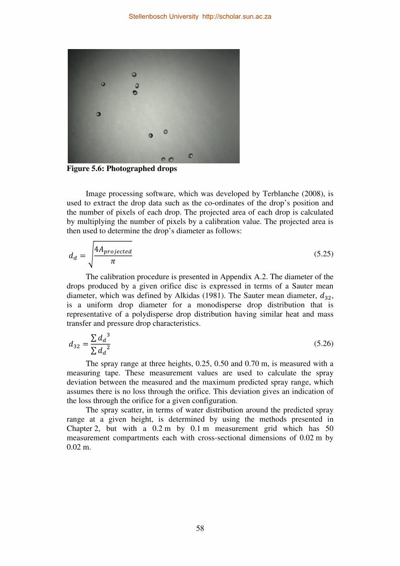
58

Figure 5.6: Photographed drops

Image processing software, which was developed by Terblanche (2008), is

used to extract the drop data such as the co-ordinates of the drop’s position and the number of pixels of each drop. The projected area of each drop is calculated by multiplying the number of pixels by a calibration value. The projected area is then used to determine the drop’s diameter as follows:

5� = 4�x#q&)�&�? (5.25)

The calibration procedure is presented in Appendix A.2. The diameter of the drops produced by a given orifice disc is expressed in terms of a Sauter mean diameter, which was defined by Alkidas (1981). The Sauter mean diameter, 5P0, is a uniform drop diameter for a monodisperse drop distribution that is representative of a polydisperse drop distribution having similar heat and mass transfer and pressure drop characteristics.

5P0 = ∑5�P∑5�0 (5.26)

The spray range at three heights, 0.25, 0.50 and 0.70 m, is measured with a measuring tape. These measurement values are used to calculate the spray deviation between the measured and the maximum predicted spray range, which assumes there is no loss through the orifice. This deviation gives an indication of the loss through the orifice for a given configuration.

The spray scatter, in terms of water distribution around the predicted spray range at a given height, is determined by using the methods presented in Chapter 2, but with a 0.2 m by 0.1 m measurement grid which has 50 measurement compartments each with cross-sectional dimensions of 0.02 m by 0.02 m.


59

5.3.3 Test procedure

The test procedure to determine the drop size, spray scatter and orifice loss coefficient are as follows:

1. Insert an orifice disc into the union fitting of the orifice nozzle chamber. 2. Set the apparatus to the desired spray angle. 3. Set the pressure head through adjusting the control valve. 4. Position the camera, lighting and glass screen to the correct height below

the orifice nozzle. 5. Record the spray range. 6. Ensure that the camera settings are correct (shutter speed of 1/8000 and an

F-stop value that best suits the lighting). 7. Focus the camera on the falling drops. 8. Take a calibration photo. 9. Switch the backlights on and capture the images. 10. Load the images into the image processing software and export the data

for processing. 11. Determine the spray range deviation for the given drop size obtained from

the photos and the measured spray range. 12. Adjust the parameter under investigation and repeat steps 9 to 11.

5.4 Orifice nozzle test results

This section presents the test results for the orifice nozzle testing in term of the Sauter mean drop diameter, the spray range deviation and spray scatter as a function of pressure head, spray angle, spray height, orifice diameter and wall thickness. The effect of bypass flow on the trajectory is also discussed.

5.4.1 Drop diameter

The Sauter mean drop diameters produced by the orifice nozzle measured at various pressure heads, spray angles, heights below the orifice, orifice diameters and wall thicknesses are presented in this section.

Orifice discs with varying thicknesses were manufactured and holes were drilled with a 1 and 2 mm drill bit. The produced orifice diameter was measured with an electronic microscope and it was found that the orifice diameter was on average 1.1 times the drill bit diameter, thus 5#x 5�x�%%��⁄ ≈ 1.1.

Rayleigh (1878) stated that the drop diameter produced by an orifice nozzle is approximately 1.9 times the orifice diameter, thus 5� 5#x⁄ ≈ 1.9. The results correspond well with this statement, as shown in Figure 5.7.


60

(a) Effect of pressure head on drop diameter

(b) Effect of spray angle on drop diameter

(c) Effect of the height below the orifice on drop diameter

(d) Effect of orifice diameter and wall thickness on drop diameter

Figure 5.7: Test results for the drop diameters produced by an orifice nozzle

The holes of a 1 mm and 2 mm orifice were tapered next to investigate the

influence of this on the drop diameter. The orifice discs were tested with a 60° tapered hole pointing towards the flow direction as well as away from the flow direction, as shown in Figure 5.8.

1.5

1.6

1.7

1.8

1.9

2.0

2.1

0.0 0.2 0.4 0.6 0.8

d3

2 /

dor

Pressure head (m)

MeasuredAverageRayleigh (1878)

1.5

1.6

1.7

1.8

1.9

2.0

2.1

-45 -30 -15 0 15 30

d3

2 /

dor

Spray angle (°)


1.5

1.6

1.7

1.8

1.9

2.0

2.1

0.2 0.4 0.6 0.8

d3

2 /

dor

Heigth below orifice (m)


1.5

1.6

1.7

1.8

1.9

2.0

2.1

0 2 4 6 8 10

d3

2 /

dor

tw/dor

Ø ≈ 1 mmØ ≈ 2 mmAverageRayleigh (1878)


61

(a) Directed inwards (b) Directed outwards

Figure 5.8: Tapered orifices directions

The results indicated that 5� 5#x⁄ ≈ 1.65. The drop diameter relative to the

jet diameter is found to be 5� 5q&�⁄ ≈ 2.10. The results are presented in Table 5-1.

Table 5-1: Test results for the drop diameters produce by a tapered orifice

nozzle

Tapered direction f¡(mm) ¢i£(mm) (mm) ¢i£¤ f¡k

Inward 1.15 0.90 1.83 2.04 1.59 1.90 1.50 3.20 2.14 1.70

Outward 1.15 0.90 1.95 2.18 1.68 1.90 1.50 3.10 2.07 1.63

It was found that the jet was unstable for the cases when the tapered hole is

directed inwards, thus affecting the spray range significantly. Thus the case with the inwards-directed orifice is not viable since it is required to accurately predict the spray range.

5.4.2 Spray range deviation

The spray range deviation for various pressure heads, spray angles, heights below the nozzle, orifice diameters and wall thicknesses are presented in this section. The results are shown in Figure 5.9.

Flow direction Flow direction


62

(a) Effect of pressure head on the spray range deviation

(b) Effect of spray angle on the spray range deviation

(c) Effect of the height below the orifice on the spray range deviation

(d) Effect of orifice diameter and wall thickness on the spray range deviation

Figure 5.9: Test results for the spray range deviation

Figure 5.9 shows that the spray range deviation is significantly impacted by

the pressure head and wall thickness, as shown in (a) and (d), but the effect of height below the orifice and spray angle is minimal, as shown in (b) and (c). This indicates that the loss through the orifice increases with an increase in pressure head, and thus velocity, and wall thickness, which is expected.

The spray range deviation for various pressure heads and heights below the orifice for a 1 and 2 mm tapered hole which is directed outwards are presented in Figure 5.10. The effect of the wall thickness can be ignored for this case since "¥ 5#x ≈ 0⁄ .

-10%

-5%

0%

5%

10%

0.0 0.2 0.4 0.6 0.8

Sp

ray r

ange

dev

iati

on

Pressure head (m)

-10%

-5%

0%

5%

10%

-30 -15 0 15 30

Sp

ray r

ange

dev

iati

on

Initial spray angle (°)

-10%

-5%

0%

5%

10%

0.2 0.4 0.6 0.8

Spra

y r

ange

dev

iati

on

Height below orifice (m)

-30%

-20%

-10%

0%

10%

0 2 4 6 8 10

Spra

y r

ange

dev

iati

on

tw / dor

Ø ≈ 1 mm

Ø ≈ 2 mm


63

Figure 5.10: Spray range deviation for a tapered hole

It can be seen from Figure 5.10 that the spray range can be predicted within

a 5 % deviation band for an outward directed tapered orifice.

5.4.3 Spray scatter

The spray scatter, or water distribution in terms of mass flux, for a tapered orifice that is directed outwards are presented in this section. Tests were conducted for various pressure heads, spray heights, spray angles and orifice sizes. Figure 5.11 shows the spray scatter produced by a 1 mm orifice with a spray angle of 0° at various pressure heads and spray heights.

(a) Spray scatter at a spray height of 0.25 m

(b) Spray scatter at a spray height of 0.50 m

-10%

-5%

0%

5%

10%

0.0 0.1 0.2 0.3 0.4 0.5 0.6 0.7 0.8 0.9 1.0

Sp

ray r

ange

dev

iati

on

Pressure head (m)

Ø ≈ 1 mm, z = 0.25 mØ ≈ 1 mm, z = 0.50 mØ ≈ 1 mm, z = 0.68 mØ ≈ 2 mm, z = 0.25 mØ ≈ 2 mm, z = 0.50 mØ ≈ 2 mm, z = 0.68 m

0

1

2

3

4

5

6

0.2 0.4 0.6 0.8 1.0 1.2 1.4

Gw

(kg/m

2s)

x (m)

H = 0.26 mH = 0.45 mH = 0.75 m

0

1

2

3

4

5

6

0.2 0.4 0.6 0.8 1.0 1.2 1.4

Gw

(kg/m

2s)

x (m)

H = 0.27 mH = 0.45 mH = 0.75 m


64

(c) Spray scatter at a spray height of 0.69 m

Figure 5.11: Spray scatter produced by a tapered 1 mm orifice with a spray

angle of 0° at various pressure heads and spray heights

The results show that the spray scatter remains constant and is fairly

concentrated at a point for various pressure heads, thus the pressure head does not influence the spray scatter significantly. The spray height merely shifts the graphs to the right, as the spray range is increased.

The effect of spray angle on the spray scatter is shown in Figure 5.12. The spray scatter produced by a 1 mm orifice with a pressure head of 0.45 m at various spray angles and spray heights are presented.

(a) Spray scatter at a spray height of 0.25 m

(b) Spray scatter at a spray height of 0.50 m

0

1

2

3

4

5

6

0.2 0.4 0.6 0.8 1.0 1.2 1.4

Gw

(kg/m

2s)

x (m)

H = 0.26 mH = 0.45 mH = 0.75 m

0

1

2

3

4

5

6

0.2 0.4 0.6 0.8 1.0 1.2 1.4

Gw

(kg/m

2s)

x (m)

θ = -45°θ = -30°θ = -15°θ = 0°θ = 15°θ = 30°

0

1

2

3

4

5

6

0.2 0.4 0.6 0.8 1.0 1.2 1.4

Gw

(kg/m

2s)

x (m)

θ = -45°θ = -30°θ = -15°θ = 0°θ = 15°θ = 30°


65

(c) Spray scatter at a spray height of 0.69 m

Figure 5.12: Spray scatter produced by a tapered 1 mm orifice with a

pressure head of 0.45 m at various spray angles and spray heights

Figure 5.12 shows that the spray scatter remains concentrated when the

spray angles are less than horizontal and it is distributed over a larger distance once the spray is directed upwards. The maximum distance over which the spray is scattered is approximately 0.12 m at a spray angle of 30 °.

Figure 5.13 shows a similar trend for a tapered 2 mm orifice at a spray height of 0.5 m.

(a) Spray scatter with a spray angle of 0° and various pressure heads

(b) Spray scatter with a pressure head of 0.45 m and various spray angles

Figure 5.13: Spray scatter produced by a tapered 2 mm orifice with a spray

height of 0.5 m

0

1

2

3

4

5

6

0.2 0.4 0.6 0.8 1.0 1.2 1.4

Gw

(kg/m

2s)

x (m)

θ = -45°θ = -30°θ = -15°θ = 0°θ = 15°θ = 30°

0

4

8

12

16

0.2 0.4 0.6 0.8 1.0 1.2 1.4

Gw

(kg/m

2s)

x (m)

H = 0.26 mH = 0.45 mH = 0.75 m

0

4

8

12

16

0.2 0.4 0.6 0.8 1.0 1.2 1.4

Gw

(kg/m

2s)

x (m)

θ = -45°θ = -30°θ = -15°θ = 0°θ = 15°θ = 30°


66

5.4.4 Bypass flow

The effect of flow over an orifice nozzle, or bypass flow on the spray trajectory is discussed in this section. The bypass flow causes an additional velocity component in the axial direction, or y – direction, of the pipe. The relationship between this velocity component and the velocity in the pipe is experimentally investigated.

The experimental setup consisted of a 32 mm PVC pipe with a tapered hole drilled in it. A control valve which is located downstream of the hole regulated the bypass flow rate and thus the velocity in the pipe. The bypass flow rate is determined by means of measuring the filling time for a predetermined volume. A grid is created in order to measure the spray deviation in the y – direction. The deviation is measured for various bypass flow rates, pressure heads, spray heights and hole diameters. The corresponding y – direction velocity component of the drop as it exits the hole for each case is determined by means of the drop model. The results for a 2.15 mm hole at various pressure heads and heights are shown in Figure 5.14.

Figure 5.14: Relationship of the y – direction velocity component and the pipe

velocity for a 2.15 mm tapered hole

It can be seen that the y – direction velocity component of the drop as it

exits the hole is just a function of the velocity in the pipe and is not influenced by the pressure head and spray height. Figure 5.15 shows this relationship for various hole sizes.

0.0

0.1

0.2

0.3

0.4

0.5

0.0 0.1 0.2 0.3 0.4 0.5

vy

(m/s

)

vpipe (m/s)

H ≈ 0.25 m, h ≈ 0.25 mH ≈ 0.25 m, h ≈ 0.50 mH ≈ 0.25 m, h ≈ 0.75 mH ≈ 0.50 m, h ≈ 0.25 mH ≈ 0.50 m, h ≈ 0.50 mH ≈ 0.50 m, h ≈ 0.75 mH ≈ 0.75 m, h ≈ 0.25 mH ≈ 0.75 m, h ≈ 0.50 mH ≈ 0.75 m, h ≈ 0.75 m


67

Figure 5.15: Relationship of the y – direction velocity component and the

pipe velocity for various hole diameters

Figure 5.15 indicates that there is a linear relationship between the y –

direction velocity component and the velocity in the pipe. The linear relationship for the 3 and 4 mm holes are similar but it is higher for the 2 mm hole. This can be due to manufacturing and measurement errors. The results indicate that it would be fair to assume that /� ≈ /��&.

The experimental investigation was scaled up to a 125 mm PVC pipe with a maximum pipe velocity of approximately 1 m/s and the results indicated a similar trend.

5.5 Spray nozzle designs

This section presents two spray nozzle designs which comprise various orifice nozzles located at predetermined positions and angles in order to deliver a predictable water distribution pattern. For the first nozzle design the orifice nozzles are positioned along a cylinder, such as a PVC pipe, and for the second nozzle design the orifice nozzles are positioned on a sphere. The design parameters of each nozzle and the manufacturing process are discussed. The measured water distribution pattern for each nozzle is presented where after the nozzles are evaluated in terms of operation within a cooling tower. The nozzles are also compared to the other commercial spray nozzles tested in this thesis.

5.5.1 Design

The two spray nozzles are designed by means of the drop model and experimental test results of a single orifice nozzle presented in the previous section. Drop diameters are assumed to be 1.9 times the orifice diameter for the design process. Schematics of both nozzle designs are shown in Figure 5.16.

0.0

0.1

0.2

0.3

0.4

0.5

0.0 0.1 0.2 0.3 0.4 0.5

vy

(m/s

)

vpipe (m/s)

Ø ≈ 2 mmØ ≈ 3 mmØ ≈ 4 mmEmpirical curveEmpirical curve (-10 %)Empirical curve (+10 %)


68

(a) Pipe spray nozzle (b) Sphere spray nozzle

Figure 5.16: Schematic of a pipe and sphere spray nozzle

The pipe sprayer consists of a 160 mm PVC class 4 pipe which has a wall

thickness of 3.45 mm. Outward tapered orifice nozzles are drilled in it by means of a 1.6 mm centre drill bit, which results in an orifice diameter of 1.76 mm. The design operating pressure head and spray height is 0.5 m from the pipe centreline respectively.

The total spray area per meter pipe of a pipe spray nozzle is expressed as

<,��x��& = 24��x��,8�� (5.27)

where 4��x�� is the spray distance of an orifice from the pipe centreline.

The number of orifice nozzles in the axial and radial directions respectively of the pipe are calculated from:

E#x,��% = 4��%E#x24��x��,8�� (5.28)

E#x,x��% = 24��x��,8��E#x4��% (5.29)

The spacing of the spray deposit positions are then calculated from:

~��x��& = 24��x��,8��E#x,x��% − 1 = 4��%E#x,��% − 1 (5.30)

The number of orifice nozzles is limited to 6 per measurement cup to ensure that the water distribution pattern can accurately be measured. This results in a mass flux of approximately 3.4 kg/m2s for the 0.01 m2 spray area of a measurement compartment. The designed maximum spray distance is 0.9 m.

The design parameters are used as input values for the drop model which then calculates the angle at which each orifice nozzle are to be placed. The holes are drilled with a milling machine in an attempt to increase the accuracy. Figure 5.17 shows a photo of the pipe spray nozzle in operation.

PVC Pipe

Hollow sphere

Orifice nozzle

Saddle adapter

Pipe saddle


69

The hole diameters of a single row of orifice nozzles are then investigated and measured by means of an electronic microscope to determine the accuracy of the manufacturing.

Figure 5.17: Pipe spray nozzle in operation

The sphere sprayer consists of a plastic ball, taken from a ball valve, which has a 155 mm outside diameter and a shell thickness of 2.5 mm. The ball is cut in half and fitted to an adapter which screws into the header pipe. Straight orifice nozzles with a diameter of 2 mm are cut through the shell by means of a 5-axis CNC machine. The design operating pressure head and spray height are 1.0 m and 0.5 m from the position where the sphere is cut respectively.

The total spray area of a sphere spray nozzle is expressed as:

<,��x��m&x& = 24��x��,8��0 (5.31)

where the maximum spray distance is equal to the half of the diagonal of the

square spray pattern, thus 4�¦(�x&��& = √24��x��,8��.

The spacing of the spray deposit positions are calculated from:

~��x��m&x& = √24��x��,8��E#x − 1 (5.32)

The sprayer is designed to produce a 1.0 m square spray pattern, if the orifice loss is ignored (; = 0), with a spray deposited at intervals of every 50 mm, which is equivalent to 441 trajectories within the 1.0 m2. This results in an approximate mass flux of 4.4 kg/m2s.

The design parameters are once again used as input values for the drop model which then calculates the angle at which each orifice nozzle are to be placed. Figure 5.18 shows a photo of the sphere spray nozzle in operation.


70

Figure 5.18: Sphere spray nozzle in operation

The design procedure are shown in Figure 5.19.

Input parameters

Aspray, Gw, dor, H, h

Number of orifices

nor Eq. (5.24)

Pipe spray nozzle

Sphere spray nozzle

Maximum spray length Lspray, max

Eq. (5.27)

Maximum spray length Lspray, max

Eq. (5.31)

Number of axial and radial orifices nor, axial, nor, radial

Eq. (5.28), Eq. (5.29)

Orifice spacing Sspray sphere Eq. (5.32)

Orifice spacing Sspray pipe

Eq. (5.30)

Spray grid

Spray angle for each orifice

Eq. (5.23) Figure 5.19: Design procedure


71

5.5.2 Water distribution patterns

The water distribution pattern of each nozzle design is measured in the test facility discussed in Chapter 2. The measured spray patterns of the pipe sprayer are shown in Figure 5.20, where the pipe centreline coincides with the A = 0B axis. It can be seen that the water distribution fluctuates, especially in the region of @ = 0.2B, A = 0.7B, where it is increased by 90 %. This indicates that the orifices' diameter which sprays in this region is approximately 37 % larger. The average measured mass flux over the test area is 4.3 kg/m2s, which is 30 % higher than predicted. The Christiansen coefficient over the spray region is 0.69.

(a) Flow deviation contour plot (b) Mass flux graph Figure 5.20: Pipe spray nozzle water distribution pattern

The measured water distribution pattern for a row of orifice nozzles is

presented in Figure 5.21 and it is compared to the predicted water distribution based on a uniform hole diameter of 1.76 mm and on the actual measured orifice diameters.

It can be seen that the water distribution can accurately be predicted, but poor accuracy and repeatability in the manufacturing process causes the orifice diameter to vary and thus varying the mass flow rate.

x (m)

y (

m)

0 0.1 0.2 0.3

0

0.1

0.2

0.3

0.4

0.5

0.6

0.7

0.8

0.9

%

-100-90-80-70-60-50-40-30-20-100102030405060708090100

0

1

2

3

4

5

6

7

8

9

10

0.0 0.2 0.4 0.6 0.8 1.0

Gw

(kg/m

2s)

y-direction (m)

x = 0.0 mx = 0.1 mx = 0.2 mx = 0.3 mPredicted


72

Figure 5.21: Measured and predicted water distribution patterns for a single

row of orifice nozzles

To investigate the effect of poor manufacturing through drilling of the

orifice nozzles, the pipe spray nozzle was manufactured by laser cutting, which has a much higher accuracy and repeatability than drilling by hand. The pipe nozzle was manufactured from a 0.9 mm steel sheet and rolled into a pipe. The measured water distribution pattern produced by this pipe nozzle is shown in Figure 5.22. It can be seen that the water distribution is uniform, with a Christiansen coefficient of 0.94 over the test area, which is near perfect. The measured average mass flux is 3.45 kg/m2s, which is similar to the predicted value of 3.4 kg/m2s.

(a) Flow deviation contour plot (b) Mass flux graph Figure 5.22: Laser cut pipe spray nozzle water distribution pattern

The measured spray pattern of the sphere sprayer is shown in Figure 5.23,

where the sphere centre coincides with the @ = 0B, A = 0B axis. Figure 5.23 (a)

0

1

2

3

4

5

6

7

8

9

10

0.0 0.1 0.2 0.3 0.4 0.5 0.6 0.7 0.8 0.9 1.0

m (

kg/s

) ×

10

3

Radial distance (m)

Measured

Predicted (Uniform diameters)

Predicted (Measured diameters)

x (m)

y (

m)

0 0.1 0.2 0.3

0

0.1

0.2

0.3

0.4

0.5

0.6

0.7

0.8

0.9

%

-100-90-80-70-60-50-40-30-20-100102030405060708090100

0

1

2

3

4

5

6

7

8

9

10

0.0 0.2 0.4 0.6 0.8 1.0

Gw

(kg/m

2s)

y-direction (m)

x = 0.0 mx = 0.1 mx = 0.2 mx = 0.3 mPredicted


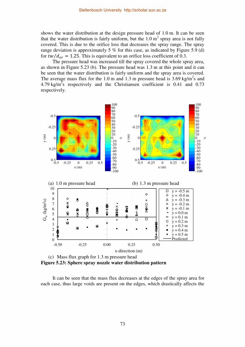
73

shows the water distribution at the design pressure head of 1.0 m. It can be seen that the water distribution is fairly uniform, but the 1.0 m2 spray area is not fully covered. This is due to the orifice loss that decreases the spray range. The spray range deviation is approximately 5 % for this case, as indicated by Figure 5.9 (d) for "¥ 5#x = 1.25⁄ . This is equivalent to an orifice loss coefficient of 0.3.

The pressure head was increased till the spray covered the whole spray area, as shown in Figure 5.23 (b). The pressure head was 1.3 m at this point and it can be seen that the water distribution is fairly uniform and the spray area is covered. The average mass flux for the 1.0 m and 1.3 m pressure head is 3.69 kg/m2s and 4.79 kg/m2s respectively and the Christiansen coefficient is 0.41 and 0.73 respectively.

(a) 1.0 m pressure head (b) 1.3 m pressure head

(c) Mass flux graph for 1.3 m pressure head

Figure 5.23: Sphere spray nozzle water distribution pattern

It can be seen that the mass flux decreases at the edges of the spray area for

each case, thus large voids are present on the edges, which drastically affects the

x (m)

y (

m)

-0.5 -0.25 0 0.25 0.5

-0.5

-0.25

0

0.25

0.5

%

-100-90-80-70-60-50-40-30-20-100102030405060708090100

x (m)

y (

m)

-0.5 -0.25 0 0.25 0.5

-0.5

-0.25

0

0.25

0.5

%

-100-90-80-70-60-50-40-30-20-100102030405060708090100

0

1

2

3

4

5

6

7

8

9

10

-0.50 -0.25 0.00 0.25 0.50

Gw

(kg/m

2s)

x-direction (m)

y = -0.5 my = -0.4 my = -0.3 my = -0.2 my = -0.1 my = 0.0 my = 0.1 my = 0.2 my = 0.3 my = 0.4 my = 0.5 mPredicted


74

Christiansen coefficient. The Christiansen coefficient over the 0.8 m by 0.8 m area is 0.81 for a 1.0 m pressure head and 0.86 for a 1.3 m pressure head.

The decrease in mass flux at the edges might be due to flow circulation within the sphere, which could cause pressure variations which affects the spray range of the orifice nozzles. The spray deposit grid positions does not always match up with the measurement grid, which also effects the measured water distribution pattern.

The water distribution pattern results for the spray nozzles are summarised in Table 5-2. It is evident that the uniformity of the water distribution is dependent on the accuracy and repeatability of the manufacturing process.

Table 5-2: Water distribution pattern test results

Average mass flux, ¨©DDDD (kg/m2s) Christiansen

coefficient, ª« Predicted Measured Deviation

Pipe (PVC)

3.44 4.23 24 % 0.69

Pipe (Sheet)

3.44 3.45 0 % 0.94

Sphere (H=1.3 )

4.41 4.79 9 % 0.76

5.5.3 Comparative evaluation

The pipe and sphere spray nozzles can be installed in the following manner into existing or new industrial cooling towers. Figure 5.24 shows the three possible installation configurations of the spray nozzles.

(a) As a header pipe spray nozzle, which replaces the distribution pipes of a conventional cooling tower.

(b) As a lateral pipe spray nozzle, which consists of a T-piece with two short pipe nozzle arms. This is then fitted to the distribution pipes, similar to a conventional spray nozzle, with the lateral pipe centreline perpendicular to the centreline of the distribution pipe.

(c) As a sphere spray nozzle, which is fitted to the distribution pipe similar to a conventional spray nozzle.


75

(a) Header pipe

spray nozzle (b) Lateral pipe spray nozzle (c) Sphere spray

nozzle Figure 5.24: Possible installation configurations of the spray nozzle designs

The three proposed spray nozzles have got various advantages and

disadvantages compared to each other and to commercial spray nozzles as tested previously. These advantages and disadvantages are shortly discussed. Methods to minimise or mitigate the drawbacks are provided.

• Nozzle design

All three spray nozzles have a robust and simple design, which will not be significantly affected by high temperatures and chemical attack. They can distribute the water over a large area with a minimal pressure head thus operating costs would be lower than the commercial nozzles. The spray area could be linearly adjustable with height if the orifice angles are chosen correctly, thus straight trajectories, a feature that commercial spray nozzles seldom have.

The nozzles would be susceptible to clogging, since the diameters of the orifice nozzles are relatively small. The abrasion effect of small particles in the cooling water could also alter the geometry of the orifice nozzles, which will lead to increased drop diameters and spray ranges. The orifices of commercial spray nozzles are large, thus clogging would not be experienced. The clogging and abrasion of the orifices could, however, be minimised by installing strainers within the saddle in the cases of the lateral and sphere spray nozzles.

The lateral and sphere spray nozzle is on par with the commercial spray nozzles regarding maintainability, but the header pipe spray nozzle could be problematic.

• Drops

The orifice nozzles, which all three spray nozzles incorporates, delivers drops with Sauter mean diameters approximately 1.9 times the diameter of the orifice, thus relatively small drop sizes can be produced. The diameters of the drops would be uniform and would not be affected by an increase in pressure head. No drop collisions would occur, since trajectories would not intersect. All of these features are rare in commercial spray nozzles.

• Water distribution

All three spray nozzles would deliver a near uniform square spray pattern, which size would not increase with an increase in pressure head if the trajectories are designed to be reasonably straight. No seepage below the nozzle would occur


76

and spray overlapping would not be required. The water distribution of commercial spray nozzles is often non uniform, with high water intensities directly below the nozzle. Overlapping is thus required to counter the non uniformities in the water distribution.


The main conclusions regarding spray nozzle design are summarised as follows:

• The Sauter mean drop diameter produced by an orifice nozzle is approximately 1.9 times the orifice diameter.

• The radial spray distance of an orifice nozzle can be predicted within 5 % by means of solving the equations of motion based on the assumptions made.

• The orifice nozzle produces a fairly concentrated spray pattern for various spray angles.

• The water distribution pattern can be predicted using the methods and experimental data presented in this section.

• An accurate manufacturing process with high repeatability is required, similarly to laser cutting. Plastic moulding would possibly be the best option.

• The three proposed spray nozzles would enhance the performance of cooling towers considerably.


77

6 SUMMARY AND CONCLUSIONS

The performance of spray zones in wet cooling towers was evaluated in terms of nozzle flow characteristics, friction losses and water distribution. The performance evaluation of three commercial spray nozzles that are currently being used in the wet cooling tower industry was done to obtain a better understanding of the state-of-the-art. The results indicated that the standard of commercial spray nozzles is not ideal. It was found that the performance of such a commercial spray nozzle could significantly be enhanced through minor design and installation alterations. A pipe spray nozzle was designed which delivered a predictable and near uniform water distribution. This indicated that the performance of spray zones and thus wet cooling towers can still be enhanced.

A background on wet cooling towers is provided in Chapter 1 as well as the objectives of this project. The motivation behind the research is discussed and a brief literature review is presented.

The flow characteristics, loss coefficients through and across the nozzle and the water distribution of three spray nozzles were obtained by means of an experimental procedure which was presented in Chapter 2. It was found that flow over a nozzle affects its flow characteristics and should be taken into consideration when designing a wet cooling tower. Empirical relations for the flow characteristics and losses were obtained which can be used in the design process. The results showed that two nearly identical spray nozzles can have significantly different performance characteristics. The test results of the water distribution patterns showed that the uniformity is very poor, which will directly influence the cooling performance.

The implementation of the test results obtained in Chapter 2 is discussed in Chapter 3, where the relevant theory is provided. It is showed that the water distribution of an array of spray nozzles can accurately be predicted through superpositioning of a single nozzle’s water distribution pattern.

In Chapter 4 a systematic approach is implemented to enhance the performance of a commercial spray nozzle in terms of flow characteristics and water distribution through minor alterations. The results of the initial performance evaluation are presented as well as the influence of various modifications. The improved nozzle’s flow characteristics and water distribution patterns are also showed.

A pipe and sphere spray nozzle, which comprise a standard PVC pipe and half a sphere respectively with holes located at various angles, are designed and tested in Chapter 5. The aim of the design is to be able to accurately predict the water distribution by means of a single drop trajectory model. Each hole acts as an orifice nozzle and the effect of adjusting various parameters such as pressure head, spray angle, wall thickness and orifice diameter are investigated experimentally. The water distribution test results of the final design are presented. The results show that it is possible to design and manufacture a spray nozzle that delivers a predictable water distribution pattern. An accurate and repeatable method of manufacturing the holes is, however, required. Three possible installation configurations, based on the pipe and sphere spray nozzle


78

designs, are presented. The advantages and disadvantages of these three configurations relative to each other and to commercial spray nozzles are discussed.

This project investigated the performance of spray nozzles and spray zones of wet cooling towers and found that there is still much room for improvement in terms of the predictability and uniformity of the water distribution for a given nozzle design. The two proposed spray nozzle designs which are presented would significantly enhance the performance of wet cooling tower spray zones. These improvements, however, will only be realised if further investigation, such as accurate manufacturing processes of orifices is continued.


79

REFERENCES

Alkidas, A., C. 1981. The Influence of Size-Distribution Parameters on the Evaporation of Polydisperse Dilute Sprays. International Journal of Heat and

Mass Transfer, Vol. 24, No. 12, pp. 1913 – 1923.

Bellagamba, B., Dinelli, G., Tognotti, L. and Zanelli, S. 1988. Water distribution in cooling towers: Characterization of industrial spray nozzles. International

Cooling Tower Conference. Haaland, S.E. 1983. Simple and Explicit Formulas for the Friction Factor in Turbulent Pipe Flow, International Journal of Fluids Engineering, Vol. 105,

No. 3, pp. 89 - 90.

Kranc, S.C. 1993a. Improving the Efficiency of Water Deposition Systems in Counterflow Cooling Towers. Proceedings of the American Power Conference,

Vol. 55 (2), pp. 1432 – 1437.

Kranc, S.C. 1993b. Performance of Counterflow Cooling Towers with Structured Packings and Maldistributed Water flow. Numerical Heat Transfer, Part A, Vol.

23, pp. 115 - 127.

Kranc, S.C., 2005. Optimal Spray Patterns for Counterflow Cooling Towers with Structured Packing. Applied Mathematical Modelling, Vol. 31 pp. 676 - 686. Kröger, D.G., 2004. Air-Cooled Heat Exchanger and Cooling Towers, Thermal-Flow performance Evaluation and Design. Pennwell Corp. Tulsa, OK, USA. Rayleigh, Lord, 1878. On the Instability of Jets. Proceedings of the London

Mathematical Society, Vol. 10, pp. 4 - 13. Reuter, H.C.R, Viljoen, D.J. and Kröger, D.G. 2010a. A Method to Determine the Performance Characteristics of Cooling Tower Spray Zones. Proceedings of the

14th

International Heat Transfer Conference, Vol. 14.

Reuter, H.C.R. 2010b. Performance Evaluation of Natural Draft Cooling Towers with Anisotropic Fills. PhD Dissertation, University of Stellenbosch. Terblance, R. 2008. Investigation of Performance Enhancing Devices for the Rain Zones of Wet-Cooling Towers. MScEng. Thesis, University of Stellenbosch. Tognotti, L., Zanelli, S., Bellagamba, B., Mattachini, F. and Lotti, G. 1991. Characterization and Performance of Spray Nozzles for Water Distribution in Cooling Towers. NIST, Vol. 813, pp. 787 – 795.


80

Turton, R. and Lievenspiel, O. 1986. A Short Note on the Drag Correlation for Spheres. Powder Technologies, Vol.47, pp.83 - 86.

Viljoen, D.J. 2006. Evaluation and Performance Prediction of Cooling Tower Spray Zones. MScEng. Thesis, University of Stellenbosch. Vitkovic, P., Syrovatka, V. 2009. Optimal Water Distribution in The Cooling Tower. Fournal of Flow Visualization and Image Processing, Vol. 16, pp. 367 –

375.

White, F.M. 2008. Fluid Mechanics, 6th ed. McGraw Hill, New York. Xiaoni, Q., Zhenyan, L. and Dandan, L. 2006. Performance Characteristics of a Shower Cooling Tower. Energy Conservation and Management, Vol. 48. pp. 193

– 203.


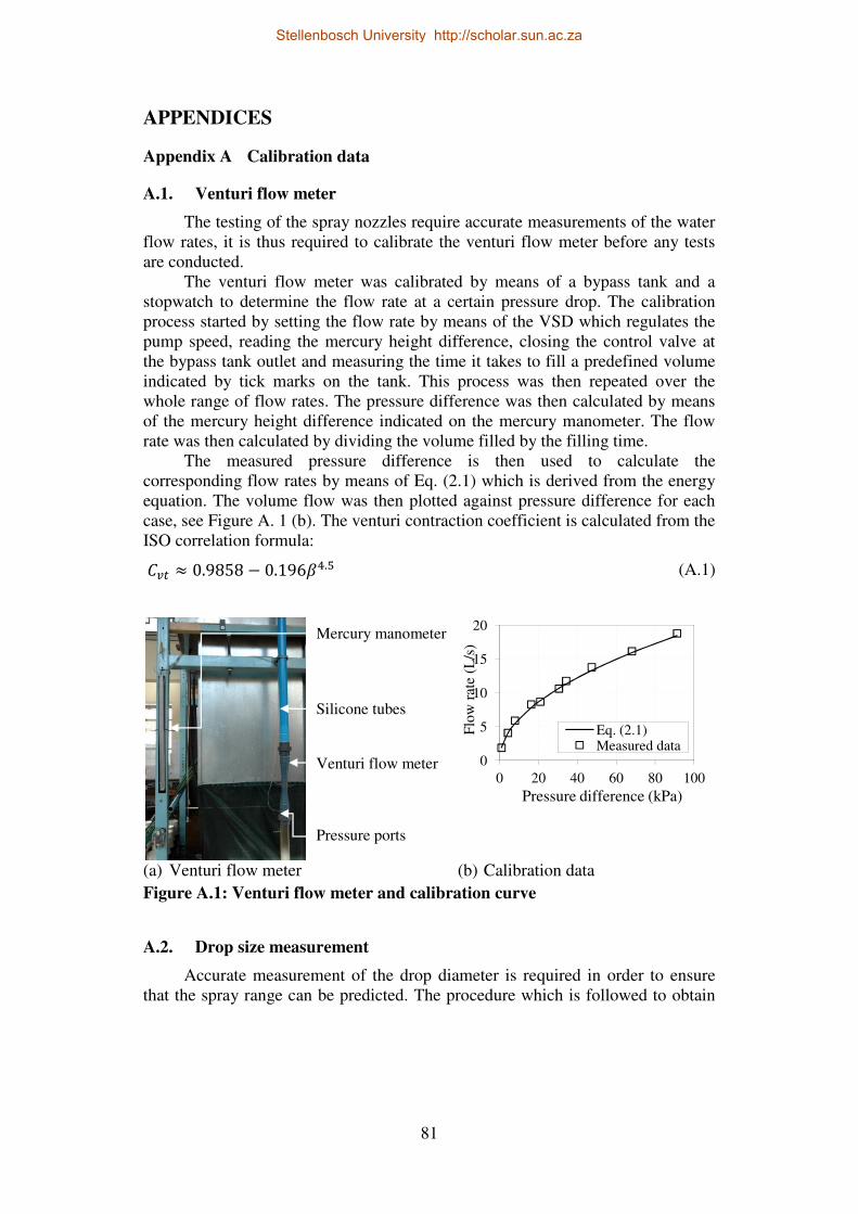
81

APPENDICES

Appendix A Calibration data

A.1. Venturi flow meter

The testing of the spray nozzles require accurate measurements of the water flow rates, it is thus required to calibrate the venturi flow meter before any tests are conducted.

The venturi flow meter was calibrated by means of a bypass tank and a stopwatch to determine the flow rate at a certain pressure drop. The calibration process started by setting the flow rate by means of the VSD which regulates the pump speed, reading the mercury height difference, closing the control valve at the bypass tank outlet and measuring the time it takes to fill a predefined volume indicated by tick marks on the tank. This process was then repeated over the whole range of flow rates. The pressure difference was then calculated by means of the mercury height difference indicated on the mercury manometer. The flow rate was then calculated by dividing the volume filled by the filling time.

The measured pressure difference is then used to calculate the corresponding flow rates by means of Eq. (2.1) which is derived from the energy equation. The volume flow was then plotted against pressure difference for each case, see Figure A. 1 (b). The venturi contraction coefficient is calculated from the ISO correlation formula:

�� ≈ 0.9858 − 0.196��.W (A.1)

(a) Venturi flow meter (b) Calibration data

Figure A.1: Venturi flow meter and calibration curve

A.2. Drop size measurement

Accurate measurement of the drop diameter is required in order to ensure that the spray range can be predicted. The procedure which is followed to obtain

0

5

10

15

20

0 20 40 60 80 100

Flo

w r

ate

(L/s

)

Pressure difference (kPa)

Eq. (2.1)Measured data

Silicone tubes

Venturi flow meter

Pressure ports

Mercury manometer


82

an accurate calibration value which is used to determine the drop diameters is discussed in this appendix.

The Nikon D70S digital SLR camera, which is used to photograph the falling drops, has a 1 Mega pixel resolution. The dimensions of the photo are 3008 pixels by 2000 pixels. A calibration photo, as shown in Figure A.2 is taken of a ruler once the camera is in the right position and focused on the drops to be photographed.

Figure A.2: Drop size calibration photo

The width of the photo can be read off by using the ruler and the size of a

pixel can be determined as follows:

4��&% = 4�m#�#�x��m3008 (A.2)

This size of the pixel can then be used to determine the area of a pixel and thus the area of a drop which consists of a number of pixels. The drop area is then used to calculate the drop diameter.


83

Appendix B Sample calculations

This appendix presents sample calculations for determining the nozzle flow characteristics, losses through and across a nozzle and water distribution patterns. A sample calculation for the single drop trajectory model is also presented.

B.1. Flow characteristics

This section presents the sample calculations for determining the nozzle flow characteristics. The measured data, taken for nozzle no.1, are given in Table B-1. Table B‒1: Sample calculation data for the flow characteristics of nozzle

no. 1

Density of water � = 998 ¬� BP⁄

Dynamic viscosity of water �� = 0.001®. p

Gravitational constant � = 9.81B p0⁄

Bucket filling mass '�#$$%&�()!&� = 10¬�

Bucket filling time ∆" = 11.31p

Header pipe diameter 5��& = 0.1531B

Piezometer head reading ℎ�,+ = 0.205B

Distance between the piezometer and nozzle inlet 4 = 0.400B

Nozzle outlet level relative to the piezometer’s base 10 = −0.2085B

The nozzle volume flow rate as given by Eq. (2.3):

��#$$%& = '�#$$%&�()!&� �∆" = 0.88 4p (B.1)

The water velocity in the header pipe as given by Eq. (2.15) since �� =��#$$%&:

/+ = 4��?5��&0 = 0.048Bp (B.2)

The Reynolds number:

QR = �/+5��&�� = 7.35 × 10P (B.3)

The Darcy friction factor as given by Eq. (2.22):


84

3 = 8.63 × 10OPP(QR)S − 7.69 × 10O0V(QR)W + 2.94 × 10O0+(QR)�− 6.12 × 10O+S(QR)P + 7.21 × 10O++(QR)0 − 4.54× 10OS(QR) + 0.14 = 1.11 × 10O+ (B.4)

The total gauge pressure at the nozzle inlet as given by Eq. (2.9):

*<,�#$$%& = �ℎ�,+ + 12 /+0 + �(1+ − 10) − 2 345��&612 /+0= 4049®

(B.5)

The total pressure head at the nozzle inlet as given by Eq. (2.10):

=�#$$%& = *<,�#$$%& �� = 0.41B (B.6)

The total pressure head at the nozzle inlet as given by Eq. (2.23):

=�#$$%& = 0.529(��#$$%&)0 = 0.41B (B.7)

B.2. Loss coefficients

This section presents the sample calculations for determining the loss coefficient through and across a nozzle. The measured data for determining the loss coefficient through a nozzle, taken for nozzle no.1, are given in Table B-2. Table B‒2: Sample calculation data for the loss coefficient through nozzle

no. 1

Nozzle orifice diameter 5#x = 0.021B

The velocity through the nozzle orifice can be calculated using the nozzle flow rate from Eq. (B.1):

/0 = 4��#$$%&?5#x0 = 2.541Bp (B.8)

The loss coefficient through the nozzle is then calculated from Eq. (2.11) and the total gauge pressure at the nozzle inlet as given by Eq. (B.5):

;�#$$%& = 2*<,�#$$%& �/00 − 1 = 0.257 (B.9)


85

The measured data for determining the loss coefficient across a nozzle, taken for nozzle no. 3 with a 26 mm orifice diameter, are given in Table B-3. Table B‒3: Sample calculation data for the loss coefficient across nozzle no. 3

assembly with 26 mm orifice diameter nozzles

Density of mercury �� = 13534 ¬� BP⁄

Venturi inlet diameter 5�� = 0.069B

Venturi throat diameter 5�� = 0.041B

Mercury manometer head difference reading ∆ℎ�� = 0.815B

Header pipe diameter 5��& = 0.119B

Piezometer head difference reading ∆ℎ� = 0.040B

Distance between the two piezometers 4� = 0.842B

Nozzle outlet level relative to the piezometer’s base 10 = −0.300B

Contraction ratio for the venturi flow meter:

� = 5��5�� = 0.594 (B.10)

Venturi flow meter discharge coefficient as given by the ISO correlation formula as presented in White (2008):

�� ≈ 0.9858 − 0.196��.W = 0.967 (B.11)

Venturi flow meter cross sectional throat area:

�� = ?5��04 = 1.32 × 10OPB0 (B.12)

The total flow rate of water flowing into the header pipe as given by Eq. (2.1):

�� =��2� �� − ��∆ℎ�� (1 − ��) = 19.13 4p (B.13)

The water velocity in the header pipe as given by Eq. (2.15):

/ = 4��?5��&0 = 1.72Bp (B.14)

The Reynolds number:

QR = �/5��&�� = 2.05 × 10W (B.15)

The Darcy friction factor as given by Eq. (2.22):


86

3 = 8.63 × 10OPP(QR)S − 7.69 × 10O0V(QR)W + 2.94 × 10O0+(QR)�− 6.12 × 10O+S(QR)P + 7.21 × 10O++(QR)0 − 4.54× 10OS(QR) + 0.14 = 1.79 × 10O0 (B.16)

The pipe friction loss coefficient can be calculated using Eq. (2.14), since /+ = /0 = / and 3+ = 30.

; = 2�∆ℎ�/0 − 34�5��& = 0.139 (B.17)

The pipe friction loss coefficient as given by Eq. (2.34):

; = −6.27 × 10O+0(QR)0 + 2.10 × 10OSQR − 0.0272 = 0.140 (B.18)

B.3. Water distribution

This section presents the sample calculations for determining the water distribution patterns. The measured data for the water distribution of nozzle no. 1 are given in Table B-4. Table B‒4: Sample calculation data for the water distribution of nozzle no. 1

Mercury manometer head difference reading ∆ℎ�� = 0.004B

Compartment mass reading '�,+ = 0.570¬�

Filling time ∆" = 60.31p

Compartment cross sectional area ),+ = 0.0099B0

Number of measurement points E = 180

Sum of the mass flux over the test area FC�,��+

= 63.57 ¬� B0p⁄

The total flow rate of water flowing into the header pipe as given by

Eq. (2.1):

�� =��2� �� − ��∆ℎ�� (1 − ��) = 1.35 4p (B.19)

The mass flow rate for the first compartment as given by Eq. (2.17):

B�,+ = '�,+∆" = 0.009 ¬�p (B.20)

The mass flux for the first measurement as given by Eq. (2.18):


87

C�,+ = B�,+),+ = 0.945 ¬�B0p (B.21)

The average mass flux for the whole test area as given by Eq. (2.19):

C�DDDD = 1EFC�,� = 0.353 ¬�B0p�+

(B.22)

The flow deviation for the first measurement as given by Eq. (2.20):

∆C�,� = C�,� − C�DDDDC�DDDD × 100% = 168% (B.23)

B.4. Single drop trajectory model

This section presents the sample calculations for the single drop trajectory model. The relevant input data and parameters are given in Table B-5. Table B‒5: Sample calculation data for the single drop trajectory model.

Air density � = 1.205 ¬� BP⁄

Air kinematic viscosity �� = 1.815 × 10OW B0 p⁄

Pressure head = = 0.5B

Counter flow air velocity /� = 0B/p

Drop diameter 5� = 0.002B

Initial spray angle � = 30° Orifice loss coefficient ; = 0

Time step ∆" = 0.001p

Initial x-position @� = 0B

Initial z-position 1� = 0B

The absolute drop velocity as given by Eq. (5.1):

/� = 2�=1 + ; = 3.132Bp (B.24)

The x- and z-components of the absolute drop velocity as given by Eq. (5.2) and (5.3):

/�� = /�cos(�) = 2.712B p⁄ (B.25)

/�$ = /�sin(�) = 1.566B p⁄ (B.26)


88

The x- and z-components and the magnitude of the relative air velocity as given by Eq. (5.4) to (5.6):

/�� = −/�� = −2.712B p⁄ (B.27)

/��$ = /� − /�$ = −1.566B p⁄ (B.28)

/�� = �/��0 + /��$0 = 3.132B p⁄ (B.29)

The relative velocity angle as given by Eq. (5.7):

Φ = atan 9/��$/��: = −2.618°®5 (B.30)

The Reynolds number as given by Eq. (5.8):

QR = �/��5�� = 416 (B.31)

The drag coefficient as given by Eq. (5.9):

�� = 24(1 + 0.173QR�.SWV)QR + 0.4131 + 16300QRO+.�� = 0.600 (B.32)

The mass of the drop as given by Eq. (5.11):

'� = 16?5�P � = 4.18 × 10OS¬� (B.33)

The body force from Eq. (5.10):

�| = '�� = 4.10 × 10OW± (B.34)

The buoyancy force is calculated as from Eq. (5.12):

�� = 16?5�P �� = 4.95 × 10O²± (B.35)

The drag force as well as its x- and z-components can then be calculated from Eq. (5.13) to (5.15):

�� = ?�� /��05�08 = 1.11 × 10OW± (B.36)

�� = ��cos(Φ) = −9.65 × 10OS± (B.37)

��$ = ��sin(Φ) = −5.57 × 10OS± (B.38)

The relative x- and z-components of the drop velocity calculated from Eq. (5.18) and (5.19):

/��.��+ = /�� + ��'� Δ" = 2.710B p⁄ (B.39)


89

/�$�.��+ = /�$� + (��$ + �� − �|)'� Δ" = 1.555B p⁄ (B.40)

The relative x- and z-components of the drop’s position calculated from Eq. (5.20) and (5.21):

@��.��+ = @�� + /�� + /��.��+2 Δ" = 0.003B (B.41)

1��.��+ = 1�� + /�$� + /�$�.��+2 Δ" = 0.002B (B.42)


Evaluation and Performance Enhancement of Cooling Tower ...

Documents

Transcript of Evaluation and Performance Enhancement of Cooling Tower ...