Vol.:(0123456789)1 3

Climate Dynamics https://doi.org/10.1007/s00382-021-05984-6

Evaluating the impact of climate change on extreme temperature and precipitation events over the Kashmir Himalaya

Shafkat Ahsan1 · M. Sultan Bhat1 · Akhtar Alam1,2  · Hakim Farooq1 · Hilal Ahmad Shiekh1

Received: 2 February 2021 / Accepted: 24 September 2021 © The Author(s) 2021

AbstractThe frequency and severity of climatic extremes is expected to escalate in the future primarily because of the increasing greenhouse gas concentrations in the atmosphere. This study aims to assess the impact of climate change on the extreme temperature and precipitation scenarios using climate indices in the Kashmir Himalaya. The analysis has been carried out for the twenty-first century under different representative concentration pathways (RCPs) through the Statistical Downscaling Model (SDSM) and ClimPACT2. The simulation reveals that the climate in the region will get progressively warmer in the future by increments of 0.36–1.48 °C and 0.65–1.07 °C in mean maximum and minimum temperatures respectively, during 2080s (2071–2100) relative to 1980–2010 under RCP8.5. The annual precipitation is likely to decrease by a maximum of 2.09–6.61% (2080s) under RCP8.5. The seasonal distribution of precipitation is expected to alter significantly with winter, spring, and summer seasons marking reductions of 9%, 5.7%, and 1.7%, respectively during 2080s under RCP8.5. The results of extreme climate evaluation show significant increasing trends for warm temperature-based indices and decreasing trends for cold temperature-based indices. Precipitation indices on the other hand show weaker and spatially incoherent trends with a general tendency towards dry regimes. The projected scenarios of extreme climate indices may result in large-scale adverse impacts on the environment and ecological resource base of the Kashmir Himalaya.

Keywords Climatic extremes · Kashmir Himalaya · Representative Concentration Pathway (RCP) · Statistical Downscaling Model (SDSM) · ClimPACT2

1 Introduction

Climate change is central to the global environmental man-agement and sustainability issues of the twenty-first cen-tury, given its implications to natural and human systems (Campbell et al. 2011; Gan et al. 2015). The perturbation of global radiation balance owing to increasing emissions of CO2 and other greenhouse gases is heating the atmosphere and causing global warming (Chu et al. 2010; Huang et al. 2011). From the perspective of climate change impacts, the most noticeable and heavily felt are the extreme weather and climate events because of their immediate and disas-trous consequences on the natural and social environment.

Climate change has enhanced the probability of temperature and precipitation extremes (Fischer et al 2013), and several studies (Orlowsky and Seneviratne 2012; Kharin et al. 2013; Sillmann et al. 2013) have projected the changing patterns of extreme climate events along with rising anthropogenic greenhouse gas emissions. The change in the frequency and magnitude of extreme weather events is also considered as an indicator of changing climate in a region (Easterling et al. 2000; Zhang et al. 2011). The study of extreme weather and climate events has attained significant attention, however, the majority of studies on long-term climate changes have focused on changes in mean values (Kostopoulou and Jones 2005; Alexander et al. 2006). This is primarily because of the lack of long-term high-quality observational data, required for the detection and attribution of the extremes (Zhang et al. 2005). Global circulation models (GCMs) provide a promising option for simulating the present and future climates and generation of long-term time-series data, which can be used to analyze the possible changes in future extreme events (Sillman and Roeckner 2008).

* Akhtar Alam akhtar.alam@ucl.ac.uk

1 Department of Geography and Disaster Management, University of Kashmir, Srinagar 190006, India

2 Institute for Risk and Disaster Reduction, University College London, Gower Street, London WC1E 6BT, UK

S. Ahsan et al.

1 3

GCMs have been the primary tools for understanding the present and future state of the climate of the planet earth. The data provided by GCMs are being used to carry out the impact studies from global to regional scales; however, the coarser grid resolution limits their direct applicability at the regional and local levels. The larger grid size of GCMs does not account for regional, sub-grid features (e.g., topog-raphy, cloud, and land use) that play a significant role in determining the local climate (Mearns et al. 2003; Coulibaly et al. 2005; Koukidis and Berg 2009). This scale mismatch is being dealt with using a wide range of dynamical and sta-tistical downscaling techniques (Nguyen et al. 2006, 2007; Fowler et al. 2007). The dynamical downscaling involves the nestling of a higher resolution Regional Climate Model (RCM) within a GCM to obtain the resolved climate sce-narios. This approach can generate the climate data at much finer scales ∼ 0.5° latitude and longitude scale (Fowler et al. 2007); however, being computationally intensive (Wilby and Wigley 1997), it has relatively restricted application in the local impact assessment studies (Hay and Clark 2003; Fowler et al. 2007). Statistical downscaling on the other hand relies upon the empirical relationships between the observed data and the large-scale predictors and has the advantages of being simple in application and also com-putationally less demanding (Samadi et al. 2013). Among the different Statistical downscaling approaches, Statisti-cal Downscaling Model (SDSM) is a popular method used globally for climate change assessment and impact studies (Wilby et al. 2002; Gagnon et al. 2005; Chu et al. 2010; Huang et al. 2011; Mahmood and Babel 2014; Zhu et al. 2019). Numerous comparative studies have pointed out the ability of SDSM to perform better than other downscaling techniques in simulating the current and future climate vari-ability with confidence (Coulibaly et al. 2005; Khan et al. 2006; Chen et  al.2011; Teutschbein et  al.2011; Samadi et al.2013). In addition to simulation of the mean climate variables, SDSM has a good capability in simulating cli-matic extremes (Hashmi et al.2010; Huang et al.2011) and thus has been adopted for the present study as well.

Numerous studies across the globe have demonstrated the increase in the magnitude, frequency, and duration of the climatic extremes in response to global warming (Trenberth 2011; Otto et al.2012; Fischer et al.2013; Morak et al.2013). In the central and south Asian region percentage of warm days/nights has increased while as there has been a decrease in cold days/nights from 1961 to 2000 over 70% of the sam-pled stations (Klein Tank et al.2006). These imprints are also well established over the Indian landmass. Kothawale et al.(2010) examined the trends in pre-monsoon tempera-ture extremes for 121 stations in India and found widespread positive trends in the frequency of hot days and nights, while negative trends were observed for cold days and nights. Sim-ilar findings were reported by Dash and Mamgain (2011)

for 1969–2005 and Revadekar et al.(2012) for 1970–2003. Joshi et al.(2020) assessed the changing patterns of hot extremes over India and reported that the frequency of hot days has augmented by 24.7% in the recent past (1976–2018) compared with the past (1951–1975). This pattern is pro-jected to continue in the future with marked increases and decreases in the frequency of hot and cold extremes respec-tively towards the end of the twenty-first century (Revadekar et al.2012). In India, the frequency of concurrent hot day and hot night (CNDHN) heat waves has increased substantially post-1984 and is projected to amplify by about 4-fold and 12-fold towards the mid-21st and end-twenty-first century respectively under RCP8.5 (Mukherjee and Mishra 2018). For the western Himalayan region, decreases have been reported in the percentage of cold nights while as there have been increases in the percentage of warm nights during the winter season (Dimri and Dash 2012). Global analysis of the precipitation-based extreme indices, on the other hand, manifests spatially heterogeneous trends with a tendency towards wetter conditions in some regions while drying trends in other regions (Donat et al.2013). Klein Tank et al.(2006) also reported the same for the central and south Asian region. From 1910 to 2000 there has been an increase in the extreme precipitation events in contagious areas from NWH in Kashmir to the Deccan plateau in India (Roy and Balling 2004). In the Hindu Kush Himalayan (HKH) region signifi-cant positive trends have been reported for light and heavy precipitation events from 1961 to 2012 (Zhan et al.2017). Similar results have been reported in the Pir-Panjal range from 1991 to 2016 (Shekhar et al.2017).

In the regional context, few studies have been carried employing SDSM for downscaling the mean temperature and precipitation (Mahmood and Babel 2014; Mahmood et al.2015; Shafiq et al.2019). Mahmood and Babel (2014) have also used SDSM for simulating some of the extreme temperature indices using the HadCM3 model and reported that there will be more warm extremes and fewer cold extremes in the future. Rashid et al.(2015) using the PRE-CIS simulations at a spatial resolution of 0.5° × 0.5° pro-jected an increase of 7.23 °C (± 1.84) °C and 4.89 (± 1.51) °C in average annual maximum and minimum temperatures over Pahalgam station from 2011 to 2098. Furthermore, the average annual maximum and minimum temperatures over Gulmarg station were projected to increase by 7.68 (± 2.01) °C and 5.88(± 1.51) °C. Gujree et al.(2017) explored the historic and future changes in extreme temperature and precipitation events for the twenty-first century using the PRECIS RCM model at a grid resolution of 50 × 50 km and reported climatic extremities over the region are growing owing to changing climate. However, in this study (Gujree et al.2017), no bias correction of model results was done using the observed climate data; essential to assess the inher-ent systematic bias (Varis et al.2004; Ines and Hansen 2006;

Evaluating the impact of climate change on extreme temperature and precipitation events over…

1 3

Christensen et al.2008; Teutschbein and Seibert 2010; Turco et al.2013). No detailed analysis has been carried out in this region earlier which assesses the spatio-temporal variations in extreme climate indices for the twenty-first century. The previous studies projecting the future climate change in the region have largely focused on changes in the mean clima-tology. However, the mean climatology smoothens a lot of information that can be pivotal in carrying out an impact assessment on the different climate-dependent natural and bio-physical sectors like agriculture, water resources, human health, etc. The present study is thus attempting to pro-vide an updated and detailed description of future climatic variations and their impact on the extreme climate indices under different climate change scenarios. While evaluating the extreme climate, the study employs the suite of indices defined by the expert team on sector-specific climate indices (ET-SCI). The study utilizes the IPCC recommended repre-sentative concentration pathways (RCPs) in projecting the changes in the mean values (RCP2.6, RCP4.5, and RCP8.5) and extreme climate indices (RCP4.5 and RCP8.5). Besides the station scale investigation, the study projects the regional dimensions of the future climate change and will serve as a baseline study for formulating the regional and sector-spe-cific adaptation strategies to mitigate the impacts of climate change in the fragile ecosystems of the Kashmir Himalaya.

2 Study area

This study is carried out for the Kashmir Himalaya that forms a substantial part of the northwest Himalaya (Fig. 1). The broad geomorphic architecture of the Kashmir Himalaya has evolved as result of collision between India and Eura-sia (Alam et al. 2015, 2017). The elevation varies between 1450 and 5500 a.m.s.l and results in microclimatic variations within the area (Fig. 1). Based on stratigraphy and eleva-tion, the region has three distinct physiographic divisions i.e., mountains, Karewas (lacustrine deposits), and the val-ley floor with a network of tributaries draining into trunk river Jhelum (Bhat et al. 2019). Although located in the subtropical latitudes the climate of the area falls under the Sub-Mediterranean type because of the orographic controls and altitudinal variations. The average mean maximum and minimum temperature of the region is 19.3 °C and 7.3 °C respectively with an average annual precipitation of about 84 cm (Husain 1987). The climate is marked by sharp sea-sonality characterized by four distinct seasons based on the mean temperature and precipitation viz., spring, summer, autumn, and winter. The precipitation mainly occurs in the form of snowfall from the westerly disturbances in the win-ter season from November to April. With some monsoon incursions into the region, the enclosing Pir-Panjal mountain

Fig. 1 Location of the study area and distribution of the CFSR and IMD stations; a India b Kashmir Himalaya

S. Ahsan et al.

1 3

range from the S-SW largely restricts the influence of sum-mer monsoon on the region.

3 Materials and methods

3.1 Observed data

The observed time-series data for the maximum temperature (Tmax), the mean minimum temperature (Tmin), and the pre-cipitation at daily and monthly scales were obtained from the Indian Meteorological Department (see Supplementary Material, S1). A quality check was done to identify the errors in the data before using it for the analysis. Negative daily precipitations were removed and both daily maximum and minimum temperatures were set to zero if daily Tmax was less than daily Tmin (e.g., Alexander et al.2006). Outliers in daily Tmax and Tmin, defined by values outside the range of four standard deviations (std) of the climatological mean of the value for the day i.e., mean ± 4 × std (Zhang et al. 2005; Alexander et al. 2006; Athar 2014) were identified and man-ually adjusted on a case to case basis to the data of neighbor-ing stations. The next quality criterion was the homogeneity check of data series to make sure that the variations in the data are caused only by the variations in climate rather than other external factors (Aguilar et al. 2003; Campozano et al. 2014) using the double-mass curve analysis (Tabari et al. 2011). Various stations had missing daily data gaps ranging from months to years; however, monthly data was available which was later utilized for the bias correction. Individual scattered missing entries were filled with multiple imputa-tion techniques using Statistical Package for the Social Sci-ences (SPSS) software. The data gaps of the range from months to years were substituted with the bias-corrected Climate Forecast System Reanalysis (CFSR) climate data.

3.2 Climate Forecast System Reanalysis (CFSR) data

CFSR climate data is valuable global data set provided by the National Centers for Environmental Prediction (NCEP) (Saha et al. 2010; Fuka et al. 2014; Dile and Srinivasan 2014). The data was downloaded for the study area using a bounding box of latitude 33.53°–34.54° N and longitude 74.25°–75.41 °E which generated the data at daily scale for 14 stations. The nearest CFSR data station (Fig. 1) was chosen to infill observed station data. Raw CFSR data suit-ability was checked statistically by plotting it against the available data of the respective stations and a systematic bias was found in the raw CFSR climate data, therefore it was imperative to correct the bias utilizing the available observed monthly data. Bias in the CFSR data was corrected using the Linear Scaling (LS) method which aims to perfectly match the monthly mean of corrected values with that of observed

ones (Lenderink et al. 2007). It operates with monthly cor-rection values based on the differences between observed and raw data using Eqs. (1) and (2)

where Tbc, m,d and Pbc,m,d are bias-corrected temperature and precipitation on dth day of m-th month and Traw,m,d and Praw,m,d are raw temperature and precipitation on the dth day of mth month. µ(.) is the mean value of the variable for mth month (Fang et al. 2015).

3.3 GCM/NCEP data

Historical and future simulated data on the predictors required for the SDSM were derived from the second-gener-ation Canadian Earth System Model (CanESM2) developed by the Canadian center for climate modeling and analysis (CCCma) (von Salzen et al. 2013; Khadka and Pathak 2016; Huang et al. 2016; Zhu et al. 2019). The model is a part of the fifth Coupled Model Inter Comparison Project (CMIP5) and is currently the only CMIP5 model for which ready-to-use SDSM predictors are available. The future modeled predictors are available for RCP2.6, RCP4.5, and RCP8.5. In addition to CanESM2 predictors, the National Centers for Environmental Prediction (NCEP) reanalysis predictors for the period 1961–2005 were used to calibrate and validate the SDSM model.

3.4 Description of SDSM model

The most popularly used downscaling model SDSM version 4.2 (Wilby and Dawson 2007) was used in this study. SDSM is a hybrid of multiple linear regression (MLR) and stochas-tic weather generator (SWG) (Meenu et al. 2013; Mahmood and Babel 2014). The SWG can generate a maximum of 100 ensembles while 20 ensembles are considered sufficient (Wilby et al. 2002; Gagnon et al. 2005; Chu et al. 2010). SDSM contains two kinds of optimization algorithms: (1) ordinary least squares (OLS) and (2) dual simplex (DS). The OLS was used because it is faster than DS and produces comparable results with DS (Huang et al. 2011). Moreover, annual and monthly sub-models can be developed during the calibration and generation of future scenarios. The annual model uses the same transfer function for 12 months while as in the monthly model 12 regression equations are devel-oped for 12 months (Huang et al. 2011). The model can be set unconditional or conditional model depending upon the nature of predictant; for temperature unconditional model is

(1)Tbc,m,d = T

raw,m,d + �

(

Tobs,m

)

− �(Traw,m)

(2)Pbc,m,d = P

raw,m,d ×

[

�

(

Pobs,m

)

�

(

Praw,m

)

]

Evaluating the impact of climate change on extreme temperature and precipitation events over…

1 3

used whereas precipitation is downscaled using a conditional model (Wilby et al. 2002; Chu et al. 2010). Unconditional models assume that regional predictors and the local pre-dictand are directly linked e.g., the temperature is depend-ent directly on the large-scale predictors. In contrast to this conditional model have an intermediate variable e.g., daily precipitation amounts or evaporation is conditioned by the probability of wet-day occurrence (Wilby et al. 2002). Since the precipitation data generally does not possess a normal distribution, SDSM provides several transformations before using it in developing regression equations (Khan et al. 2006; Huang et al. 2011). The SDSM performs a sequence of steps i.e., screening of predictors, calibration and valida-tion, and generation of future scenarios.

3.4.1 Screening of predictors

The selection of appropriate predictors is the most important step of any downscaling method (Wilby et al. 2002). This study employed a combination of the correlation matrix, partial correlation, and P-value (Gagnon et al. 2005; Huang et al. 2011; Mahmood and Babel 2014). The selection of the first predictor also called a super predictor is based on the highest correlation coefficient with the local predictant. The selection of subsequent predictors was done using the concept of percentage reduction in partial correlation (Mahmood and Babel 2014) and is given by the Eq. (3).

where PRP is the percentage reduction in partial correlation with respect to the correlation coefficient, P.r is the partial correlation coefficient of a predictor in the presence of super predictor, and R1 is the correlation coefficient between the predictor and predictants.

The predictors having P-value > 0.05 are ruled out of the selection process and the predictor with the lowest PRP is selected as the second predictor. This procedure is repeated up to the desired number of predictors. Multi-collinearity between the predictors was also taken into consideration during the selection of predictors.

3.4.2 Calibration and validation

After the selection of appropriate predictors, the model was calibrated for each of the predictants using NCEP predic-tors (Fig. 2). Both the annual and monthly sub-models were developed for evaluation and a later monthly model was selected (Mahmood and Babel 2014). The model was set unconditional for temperature while for precipitation condi-tional model was used (Wilby et al. 2002; Chu et al. 2010). Moreover, the precipitation data were transformed to the

(3)PRP =(P.r − R1)

R1

4th root to render it normal before using it for the calibra-tion (Khan et al. 2006). Explained variance and standard error were chosen as indicators of the performance of the calibration process (e.g., Huang et al. 2011, 2012; Mahmood et al. 2015). The model was validated by using independent data of 10 years for each of the meteorological stations (S2). With the calibrated models 20 ensembles were generated for Tmax, Tmin, and Prcp. for both the calibration and validation periods. Moreover (R2) was chosen to compare the simu-lated data (mean of 20 ensembles) with that of observed data (Huang et al. 2011; Mahmood et al. 2015).

3.4.3 Generation of future scenarios

The future scenarios for Tmax, Tmin, and Prcp. were gener-ated by forcing the calibrated models with the CanESM2 predictors for the RCP2.6, RCP4.5, and RCP8.5. The future period (2006–2100) was divided into 3-time slices of near future, mid future, and far future i.e., 2020s (2011–2040), 2050s (2041–2070), and 2080s (2071–2100) respectively (e.g., Mahmood and Babel 2013). A total of 20 ensembles (Gagnon et al. 2005; Chu et al. 2010) were generated for each variable. The simulated values (mean of 20 ensembles) were compared with the observed means from the baseline data (1980–2010) to calculate the magnitude of changes in Tmax, Tmin, and Prcp. during the various spans of the twenty-first century with respect to the baseline climatol-ogy (1980–2010).

3.5 Calculation of extreme climatic indices

The future daily data series of Tmax, Tmin, and Prcp. simu-lated by SDSM was used to calculate the extreme climatic indices using the ClimPACT2 model for RCP4.5 (stabili-zation scenario) and RCP8.5 (business as usual scenario). From the suite of indices, 15 temperature indices (S3) and 14 precipitation indices (S4) were selected for the present study.

3.6 Trend analysis of extreme indices

Linear trends were computed for each index to explore the variability in the magnitude of indices under a changing climate during the various spans of the twenty-first cen-tury. The magnitude of the trend was estimated using Sen’s slope estimator (Sen 1968) and the statistical significance of trends was established using Man Kendall’s tau test at con-fidence levels of 90% and 95%. The trends were calculated for the future period of 2010–2100 and also for the near future (2010–2040), mid future (2041–2070), and far future (2071–2100) to explore the variability of extremes within each period. Moreover, the regional averages were computed for each index and were also subjected to trend analysis.

S. Ahsan et al.

1 3

4 Results

4.1 Screening of predictors

The selected predictors for the downscaling temperature (Tmax, Tmin) and precipitation (Prcp.) are given in (S5 and S6) respectively. The temperature at 2 m height (temp)

was the super predictor for both Tmax and Tmin; precipita-tion being heterogeneous, the partial correlation coefficient between the predictors and predictants was generally low (e.g., Dibike and Coulibaly 2005; Hashmi et al. 2010; Huang et al. 2011) and as such the screening of predictors for down-scaling the precipitation was complex. Among the predic-tors, 500 hPa geopotential height (p500), the meridional

0

5

10

15

20

25

30

35

J F M A M J J A S O N D

Mea

n M

axim

um T

empe

ratu

re(°C

)

(a)

observed simulated

0

5

10

15

20

25

30

35

J F M A M J J A S O N D

Mea

n M

axim

um T

empe

ratu

re(°C

)

(b)

observed simulated

-5

0

5

10

15

20

J F M A M J J A S O N D

Mea

n M

inim

um T

empe

rart

ure(

°C)

(c)

observed simulated

-5

0

5

10

15

20

J F M A M J J A S O N D

Mea

n M

inim

um T

empe

ratu

re(°C

)

(d)

observed simluated

0

50

100

150

J F M A M J J A S O N DMea

n M

onth

ly P

recip

ita�o

n(m

m)

(e)

observed simulated

0

50

100

150

J F M A M J J A S O N D

Mea

n M

onth

ly P

recip

ita�o

n(m

m)

(f)

observed simulated

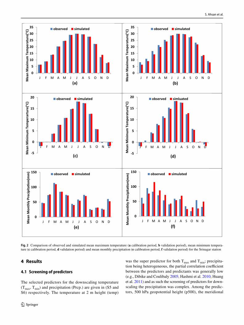
Fig. 2 Comparison of observed and simulated mean maximum temperature (a calibration period, b validation period), mean minimum tempera-ture (c calibration period, d validation period) and mean monthly precipitation (e calibration period, f validation period) for the Srinagar station

Evaluating the impact of climate change on extreme temperature and precipitation events over…

1 3

velocity component at 500 hPa (p5_v), and mean sea level pressure (Mslp) were frequent predictors for downscaling precipitation. The selected predictors for Tmax, Tmin, and Prcp. are similar to the type of predictors that have been chosen in previous studies in and around Kashmir Himalayas (Mahmood and Babel 2013, 2014; Mahmood et al. 2015; Shafiq et al. 2019).

4.2 Calibration and validation

The model was calibrated using the station-wise observed and NCEP predictors and validated for independent data of 10 years for each predictant. The percentage of explained variance E (%) and standard error (SE) were chosen as a measure of the performance of the calibrated model. E (%) for Tmax and Tmin varied between 48 and 70% and 54–66% respectively. The standard error (SE) ranged between 2.34 and 3.14 °C and 1.67–2.69 °C for Tmax and Tmin respectively. The E (%) for precipitation was generally low as compared to temperature and ranged between 12.6 and 27% with SE ranging between 0.43 and 0.51 mm. The E (%) is gener-ally low for the heterogeneous variable like daily precipi-tation amounts (Wilby et al. 2002). The R2 computed on the monthly series, varied between 94 and 97%, 93–96%, and 78–85% for Tmax, Tmin, and precipitation, respectively during the calibration period. For the validation period, R2 varied between 91 and 95% and 89–93% for Tmax and Tmin respectively whereas for precipitation it ranged between 58 and 75%. The results are well in agreement with the previous studies (Liu et al. 2008; Huang et al. 2011; Souvignet and Heinrich 2011), shown graphically for the Srinagar station (illustrative purposes) in Fig. 2 to visualize the inter-annual variations during the calibration and validation process.

4.3 Projected changes in the temperature

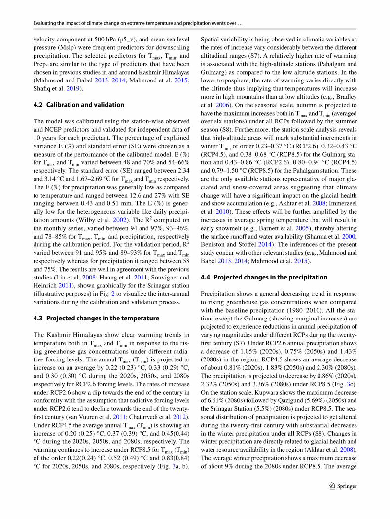
The Kashmir Himalayas show clear warming trends in temperature both in Tmax and Tmin in response to the ris-ing greenhouse gas concentrations under different radia-tive forcing levels. The annual Tmax (Tmin) is projected to increase on an average by 0.22 (0.23) °C, 0.33 (0.29) °C, and 0.30 (0.30) °C during the 2020s, 2050s, and 2080s respectively for RCP2.6 forcing levels. The rates of increase under RCP2.6 show a dip towards the end of the century in conformity with the assumption that radiative forcing levels under RCP2.6 tend to decline towards the end of the twenty-first century (van Vuuren et al. 2011; Chaturvedi et al. 2012). Under RCP4.5 the average annual Tmax (Tmin) is showing an increase of 0.20 (0.25) °C, 0.37 (0.39) °C, and 0.45(0.44) °C during the 2020s, 2050s, and 2080s, respectively. The warming continues to increase under RCP8.5 for Tmax (Tmin) of the order 0.22(0.24) °C, 0.52 (0.49) °C and 0.83(0.84) °C for 2020s, 2050s, and 2080s, respectively (Fig. 3a, b).

Spatial variability is being observed in climatic variables as the rates of increase vary considerably between the different altitudinal ranges (S7). A relatively higher rate of warming is associated with the high-altitude stations (Pahalgam and Gulmarg) as compared to the low altitude stations. In the lower troposphere, the rate of warming varies directly with the altitude thus implying that temperatures will increase more in high mountains than at low altitudes (e.g., Bradley et al. 2006). On the seasonal scale, autumn is projected to have the maximum increases both in Tmax and Tmin (averaged over six stations) under all RCPs followed by the summer season (S8). Furthermore, the station scale analysis reveals that high-altitude areas will mark substantial increments in winter Tmin of order 0.23–0.37 °C (RCP2.6), 0.32–0.43 °C (RCP4.5), and 0.38–0.68 °C (RCP8.5) for the Gulmarg sta-tion and 0.43–0.86 °C (RCP2.6), 0.80–0.94 °C (RCP4.5) and 0.79–1.50 °C (RCP8.5) for the Pahalgam station. These are the only available stations representative of major gla-ciated and snow-covered areas suggesting that climate change will have a significant impact on the glacial health and snow accumulation (e.g., Akhtar et al. 2008; Immerzeel et al. 2010). These effects will be further amplified by the increases in average spring temperature that will result in early snowmelt (e.g., Barnett et al. 2005), thereby altering the surface runoff and water availability (Sharma et al. 2000; Beniston and Stoffel 2014). The inferences of the present study concur with other relevant studies (e.g., Mahmood and Babel 2013, 2014; Mahmood et al. 2015).

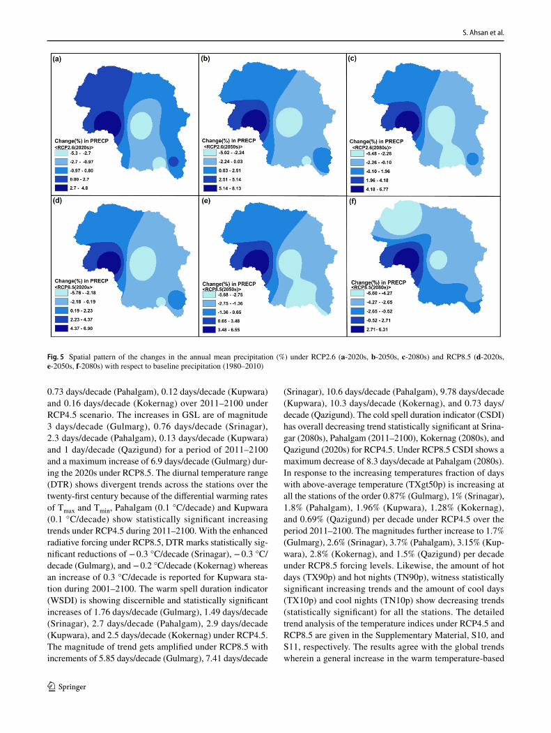
4.4 Projected changes in the precipitation

Precipitation shows a general decreasing trend in response to rising greenhouse gas concentrations when compared with the baseline precipitation (1980–2010). All the sta-tions except the Gulmarg (showing marginal increases) are projected to experience reductions in annual precipitation of varying magnitudes under different RCPs during the twenty-first century (S7). Under RCP2.6 annual precipitation shows a decrease of 1.05% (2020s), 0.75% (2050s) and 1.43% (2080s) in the region. RCP4.5 shows an average decrease of about 0.81% (2020s), 1.83% (2050s) and 2.30% (2080s). The precipitation is projected to decrease by 0.86% (2020s), 2.32% (2050s) and 3.36% (2080s) under RCP8.5 (Fig. 3c). On the station scale, Kupwara shows the maximum decrease of 6.61% (2080s) followed by Qazigund (5.69%) (2050s) and the Srinagar Station (5.5%) (2080s) under RCP8.5. The sea-sonal distribution of precipitation is projected to get altered during the twenty-first century with substantial decreases in the winter precipitation under all RCPs (S8). Changes in winter precipitation are directly related to glacial health and water resource availability in the region (Akhtar et al. 2008). The average winter precipitation shows a maximum decrease of about 9% during the 2080s under RCP8.5. The average

S. Ahsan et al.

1 3

0.00

0.10

0.20

0.30

0.40

0.50

0.60

0.70

0.80

0.90

2011-2040 2041-2070 2071-2100

Proj

eted

incr

eae

in a

nnua

l TM

AX(o C

) (a)

RCP2.6RCP4.5RCP8.5

0.00

0.10

0.20

0.30

0.40

0.50

0.60

0.70

0.80

0.90

2011-2040 2041-2070 2071-2100

Proj

ecte

d in

crea

se in

ann

ual

T MIN

(o C)

(b)

RCP2.6RCP4.5RCP8.5

-4.00

-3.50

-3.00

-2.50

-2.00

-1.50

-1.00

-0.50

0.002011-2040 2041-2070 2071-2100

Proj

ecte

d ch

ange

s in

prec

ipita

�on(

%)

(c)

RCP2.6RCP4.5RCP8.5

Fig. 3 Projected changes (averaged over six stations) in annual—TMAX (a), TMIN (b) and PRCP (c) under different RCPs

Evaluating the impact of climate change on extreme temperature and precipitation events over…

1 3

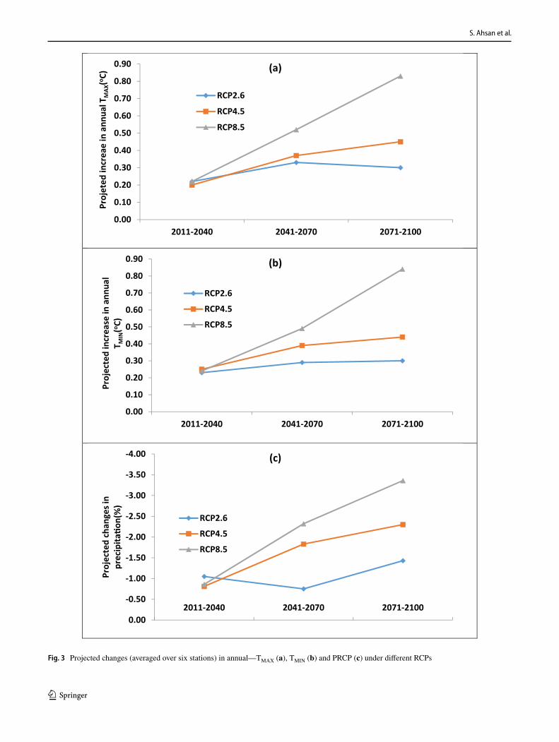
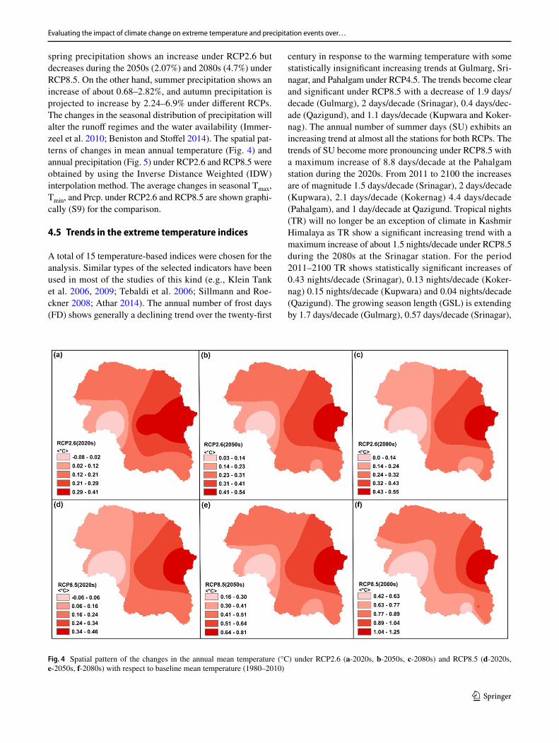
spring precipitation shows an increase under RCP2.6 but decreases during the 2050s (2.07%) and 2080s (4.7%) under RCP8.5. On the other hand, summer precipitation shows an increase of about 0.68–2.82%, and autumn precipitation is projected to increase by 2.24–6.9% under different RCPs. The changes in the seasonal distribution of precipitation will alter the runoff regimes and the water availability (Immer-zeel et al. 2010; Beniston and Stoffel 2014). The spatial pat-terns of changes in mean annual temperature (Fig. 4) and annual precipitation (Fig. 5) under RCP2.6 and RCP8.5 were obtained by using the Inverse Distance Weighted (IDW) interpolation method. The average changes in seasonal Tmax, Tmin, and Prcp. under RCP2.6 and RCP8.5 are shown graphi-cally (S9) for the comparison.

4.5 Trends in the extreme temperature indices

A total of 15 temperature-based indices were chosen for the analysis. Similar types of the selected indicators have been used in most of the studies of this kind (e.g., Klein Tank et al. 2006, 2009; Tebaldi et al. 2006; Sillmann and Roe-ckner 2008; Athar 2014). The annual number of frost days (FD) shows generally a declining trend over the twenty-first

century in response to the warming temperature with some statistically insignificant increasing trends at Gulmarg, Sri-nagar, and Pahalgam under RCP4.5. The trends become clear and significant under RCP8.5 with a decrease of 1.9 days/decade (Gulmarg), 2 days/decade (Srinagar), 0.4 days/dec-ade (Qazigund), and 1.1 days/decade (Kupwara and Koker-nag). The annual number of summer days (SU) exhibits an increasing trend at almost all the stations for both RCPs. The trends of SU become more pronouncing under RCP8.5 with a maximum increase of 8.8 days/decade at the Pahalgam station during the 2020s. From 2011 to 2100 the increases are of magnitude 1.5 days/decade (Srinagar), 2 days/decade (Kupwara), 2.1 days/decade (Kokernag) 4.4 days/decade (Pahalgam), and 1 day/decade at Qazigund. Tropical nights (TR) will no longer be an exception of climate in Kashmir Himalaya as TR show a significant increasing trend with a maximum increase of about 1.5 nights/decade under RCP8.5 during the 2080s at the Srinagar station. For the period 2011–2100 TR shows statistically significant increases of 0.43 nights/decade (Srinagar), 0.13 nights/decade (Koker-nag) 0.15 nights/decade (Kupwara) and 0.04 nights/decade (Qazigund). The growing season length (GSL) is extending by 1.7 days/decade (Gulmarg), 0.57 days/decade (Srinagar),

Fig. 4 Spatial pattern of the changes in the annual mean temperature (°C) under RCP2.6 (a-2020s, b-2050s, c-2080s) and RCP8.5 (d-2020s, e-2050s, f-2080s) with respect to baseline mean temperature (1980–2010)

S. Ahsan et al.

1 3

0.73 days/decade (Pahalgam), 0.12 days/decade (Kupwara) and 0.16 days/decade (Kokernag) over 2011–2100 under RCP4.5 scenario. The increases in GSL are of magnitude 3 days/decade (Gulmarg), 0.76 days/decade (Srinagar), 2.3 days/decade (Pahalgam), 0.13 days/decade (Kupwara) and 1 day/decade (Qazigund) for a period of 2011–2100 and a maximum increase of 6.9 days/decade (Gulmarg) dur-ing the 2020s under RCP8.5. The diurnal temperature range (DTR) shows divergent trends across the stations over the twenty-first century because of the differential warming rates of Tmax and Tmin, Pahalgam (0.1 °C/decade) and Kupwara (0.1 °C/decade) show statistically significant increasing trends under RCP4.5 during 2011–2100. With the enhanced radiative forcing under RCP8.5, DTR marks statistically sig-nificant reductions of − 0.3 °C/decade (Srinagar), − 0.3 °C/decade (Gulmarg), and − 0.2 °C/decade (Kokernag) whereas an increase of 0.3 °C/decade is reported for Kupwara sta-tion during 2001–2100. The warm spell duration indicator (WSDI) is showing discernible and statistically significant increases of 1.76 days/decade (Gulmarg), 1.49 days/decade (Srinagar), 2.7 days/decade (Pahalgam), 2.9 days/decade (Kupwara), and 2.5 days/decade (Kokernag) under RCP4.5. The magnitude of trend gets amplified under RCP8.5 with increments of 5.85 days/decade (Gulmarg), 7.41 days/decade

(Srinagar), 10.6 days/decade (Pahalgam), 9.78 days/decade (Kupwara), 10.3 days/decade (Kokernag), and 0.73 days/decade (Qazigund). The cold spell duration indicator (CSDI) has overall decreasing trend statistically significant at Srina-gar (2080s), Pahalgam (2011–2100), Kokernag (2080s), and Qazigund (2020s) for RCP4.5. Under RCP8.5 CSDI shows a maximum decrease of 8.3 days/decade at Pahalgam (2080s). In response to the increasing temperatures fraction of days with above-average temperature (TXgt50p) is increasing at all the stations of the order 0.87% (Gulmarg), 1% (Srinagar), 1.8% (Pahalgam), 1.96% (Kupwara), 1.28% (Kokernag), and 0.69% (Qazigund) per decade under RCP4.5 over the period 2011–2100. The magnitudes further increase to 1.7% (Gulmarg), 2.6% (Srinagar), 3.7% (Pahalgam), 3.15% (Kup-wara), 2.8% (Kokernag), and 1.5% (Qazigund) per decade under RCP8.5 forcing levels. Likewise, the amount of hot days (TX90p) and hot nights (TN90p), witness statistically significant increasing trends and the amount of cool days (TX10p) and cool nights (TN10p) show decreasing trends (statistically significant) for all the stations. The detailed trend analysis of the temperature indices under RCP4.5 and RCP8.5 are given in the Supplementary Material, S10, and S11, respectively. The results agree with the global trends wherein a general increase in the warm temperature-based

Fig. 5 Spatial pattern of the changes in the annual mean precipitation (%) under RCP2.6 (a-2020s, b-2050s, c-2080s) and RCP8.5 (d-2020s, e-2050s, f-2080s) with respect to baseline precipitation (1980–2010)

Evaluating the impact of climate change on extreme temperature and precipitation events over…

1 3

indices and a decrease in the cold temperature-based indices have been reported (e.g., Zhang et al. 2005; Klein Tank et al. 2006; Tebaldi et al. 2006; Sillmann and Roeckner 2008; Athar 2014).

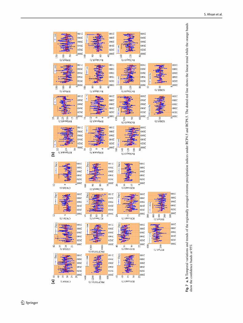
4.6 Trends in extreme precipitation indices

A total of 14 precipitation indices were selected for the analysis (Zhang et al. 2005; Tebaldi et al. 2006; Sillmann and Roeckner 2008; Athar 2014). The trends in precipitation indices are weak with only a few indices showing statisti-cally significant trends over the various spans of the twenty-first century (S12 and S13). Moreover, the trends, unlike the temperature-based indices, are spatially and temporally incoherent partly in the response to the poor performance of GCM models in resolving the local precipitation (Huang et al. 2012) and also due to greater spatio-temporal varia-tion of the precipitation in the study area. This problem has been reported in numerous other studies of this type (e.g., Kostopoulou and Jones 2005; Klein Tank et al. 2006; Vin-cent et al. 2018). Besides, the network of meteorological stations is very sparse given the optimum number of weather stations prescribed by the World Meteorological Organi-zation (WMO), and the stations are located in the differ-ent geographical and altitudinal zones thus having varied orographic and altitudinal forcing which results in strong horizontal and vertical gradients in precipitation (Yao et al. 2012; Sharma et al. 2016; Zhan et al. 2017). The maximum number of consecutive dry days (CDD) shows increas-ing trends (statistically insignificant) at Gulmarg (2020s), Srinagar (2020s), Qazigund (2020s), Pahalgam (2050s, 2011–2100), and Kupwara (2050s, 2080s) under RCP4.5. For RCP8.5 forcing levels for Gulmarg (2050s), Srinagar (2050s, 2080s), Pahalgam (2020s, 2080s) Kupwara (2050s, 2080s,) Kokernag (2080s), and Qazigund (2020s, 2050s, 2080s) show statistically insignificant increases whereas the significant positive trends were found for Pahalgam (2050s, 2011–2100) and Kupwara (2011–2100). The maxi-mum number of consecutive wet days (CWD) is showing decreasing trends at Gulmarg (2050s) (statistically sig-nificant), Kupwara (2080s), and Qazigund (2050s, 2080s) under RCP4.5. CWD shows an increasing trend (statistically insignificant) at Srinagar (2020s), Qazigund (2050s, 2080s) under RCP8.5. Annual precipitation (PRCPTOT) is show-ing a decreasing trend statistically significant at Pahalgam (2080s, 2011–2100) and Kupwara (2080s). Under RCP8.5 Kupwara shows a decrease (statistically significant) of about 6.6 mm/year during 2050s. The annual number of rainy days (rainfall > 2.5 mm) (R2.5 mm) exhibits increasing trends (statistically insignificant) for Srinagar, Kupwara (2050s), and Kokernag (2020s, 2080s, 2011–2100) while decreas-ing trends (statistically significant) were found at Kupwara (2080s, 2011–2100) under RCP4.5. Under RCP8.5 the

decreases in R2.5 mm are statistically significant for Kup-wara (2050s, 2011–2100) and Kokernag (2080s). The trends of other extreme precipitation indices of absolute thresh-olds (R10mm, R20mm), percentile-based thresholds (R95P, R99P, R95PTOT, R99PTOT), or duration based (RX1DAY, RX5DAY, RX7DAY) show a mix of increasing and decreas-ing trends without spatial coherence.

4.7 Trends in the regional average indices

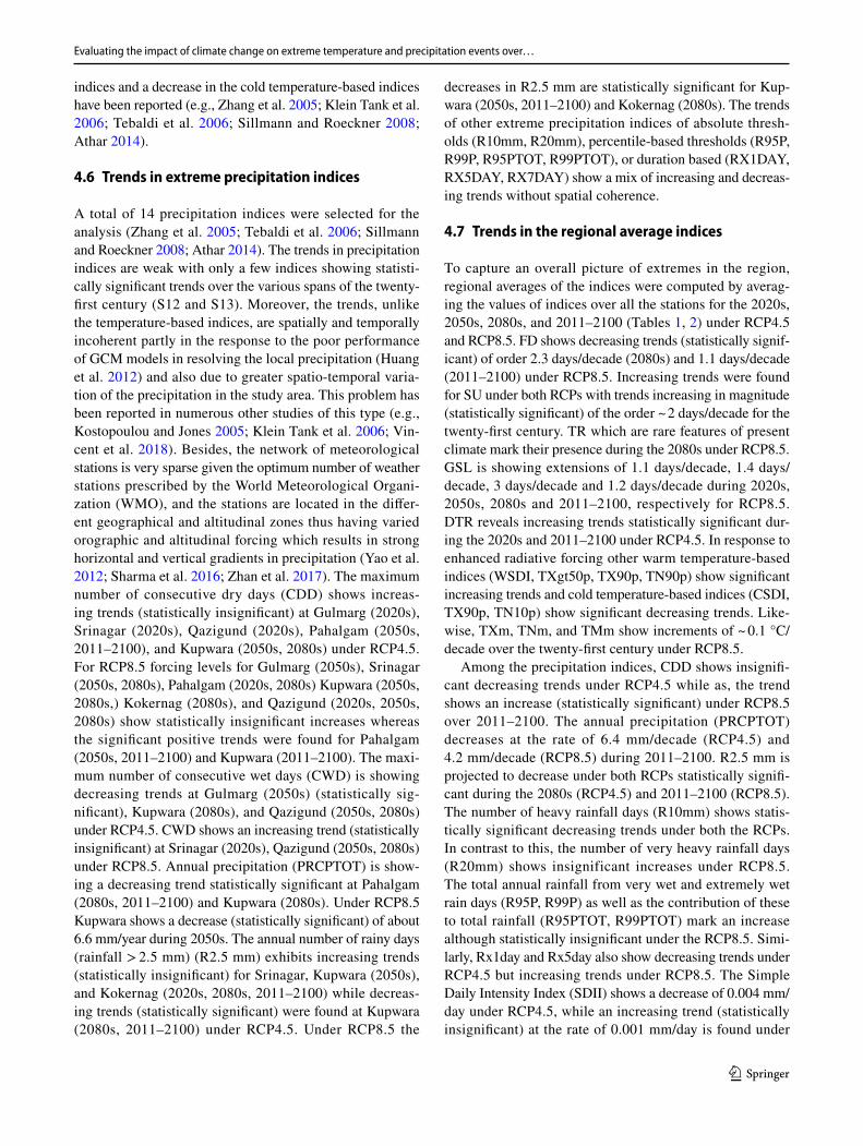
To capture an overall picture of extremes in the region, regional averages of the indices were computed by averag-ing the values of indices over all the stations for the 2020s, 2050s, 2080s, and 2011–2100 (Tables 1, 2) under RCP4.5 and RCP8.5. FD shows decreasing trends (statistically signif-icant) of order 2.3 days/decade (2080s) and 1.1 days/decade (2011–2100) under RCP8.5. Increasing trends were found for SU under both RCPs with trends increasing in magnitude (statistically significant) of the order ~ 2 days/decade for the twenty-first century. TR which are rare features of present climate mark their presence during the 2080s under RCP8.5. GSL is showing extensions of 1.1 days/decade, 1.4 days/decade, 3 days/decade and 1.2 days/decade during 2020s, 2050s, 2080s and 2011–2100, respectively for RCP8.5. DTR reveals increasing trends statistically significant dur-ing the 2020s and 2011–2100 under RCP4.5. In response to enhanced radiative forcing other warm temperature-based indices (WSDI, TXgt50p, TX90p, TN90p) show significant increasing trends and cold temperature-based indices (CSDI, TX90p, TN10p) show significant decreasing trends. Like-wise, TXm, TNm, and TMm show increments of ~ 0.1 °C/decade over the twenty-first century under RCP8.5.

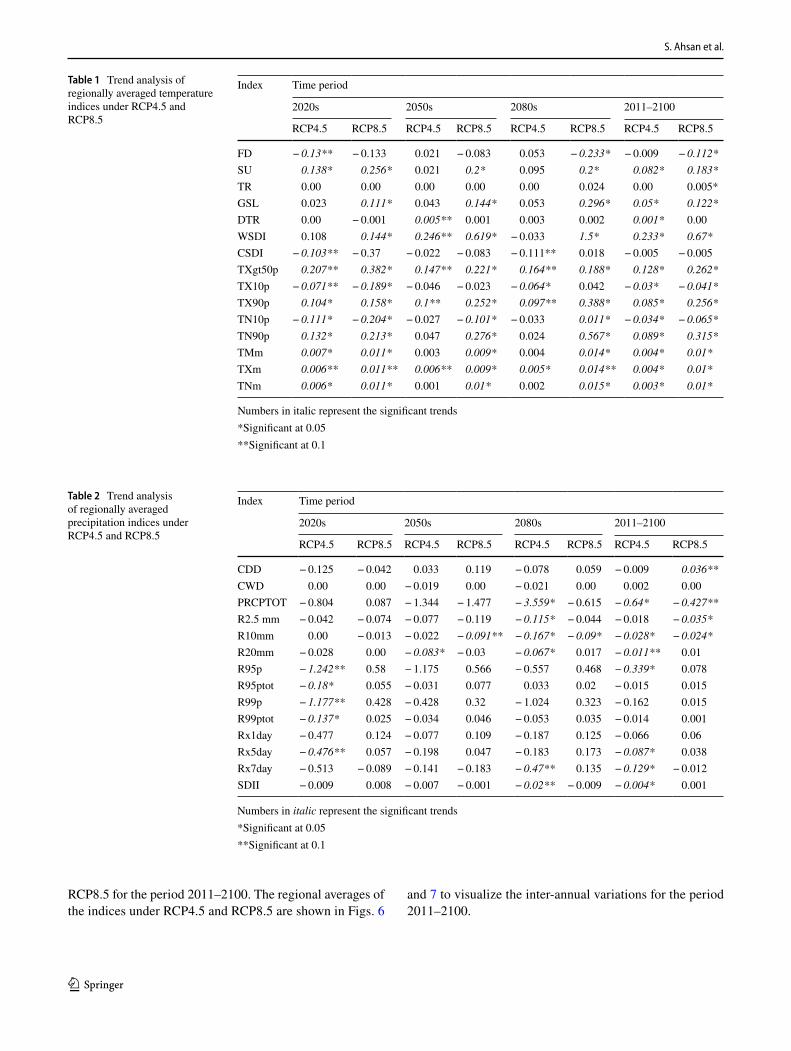
Among the precipitation indices, CDD shows insignifi-cant decreasing trends under RCP4.5 while as, the trend shows an increase (statistically significant) under RCP8.5 over 2011–2100. The annual precipitation (PRCPTOT) decreases at the rate of 6.4  mm/decade (RCP4.5) and 4.2 mm/decade (RCP8.5) during 2011–2100. R2.5 mm is projected to decrease under both RCPs statistically signifi-cant during the 2080s (RCP4.5) and 2011–2100 (RCP8.5). The number of heavy rainfall days (R10mm) shows statis-tically significant decreasing trends under both the RCPs. In contrast to this, the number of very heavy rainfall days (R20mm) shows insignificant increases under RCP8.5. The total annual rainfall from very wet and extremely wet rain days (R95P, R99P) as well as the contribution of these to total rainfall (R95PTOT, R99PTOT) mark an increase although statistically insignificant under the RCP8.5. Simi-larly, Rx1day and Rx5day also show decreasing trends under RCP4.5 but increasing trends under RCP8.5. The Simple Daily Intensity Index (SDII) shows a decrease of 0.004 mm/day under RCP4.5, while an increasing trend (statistically insignificant) at the rate of 0.001 mm/day is found under

S. Ahsan et al.

1 3

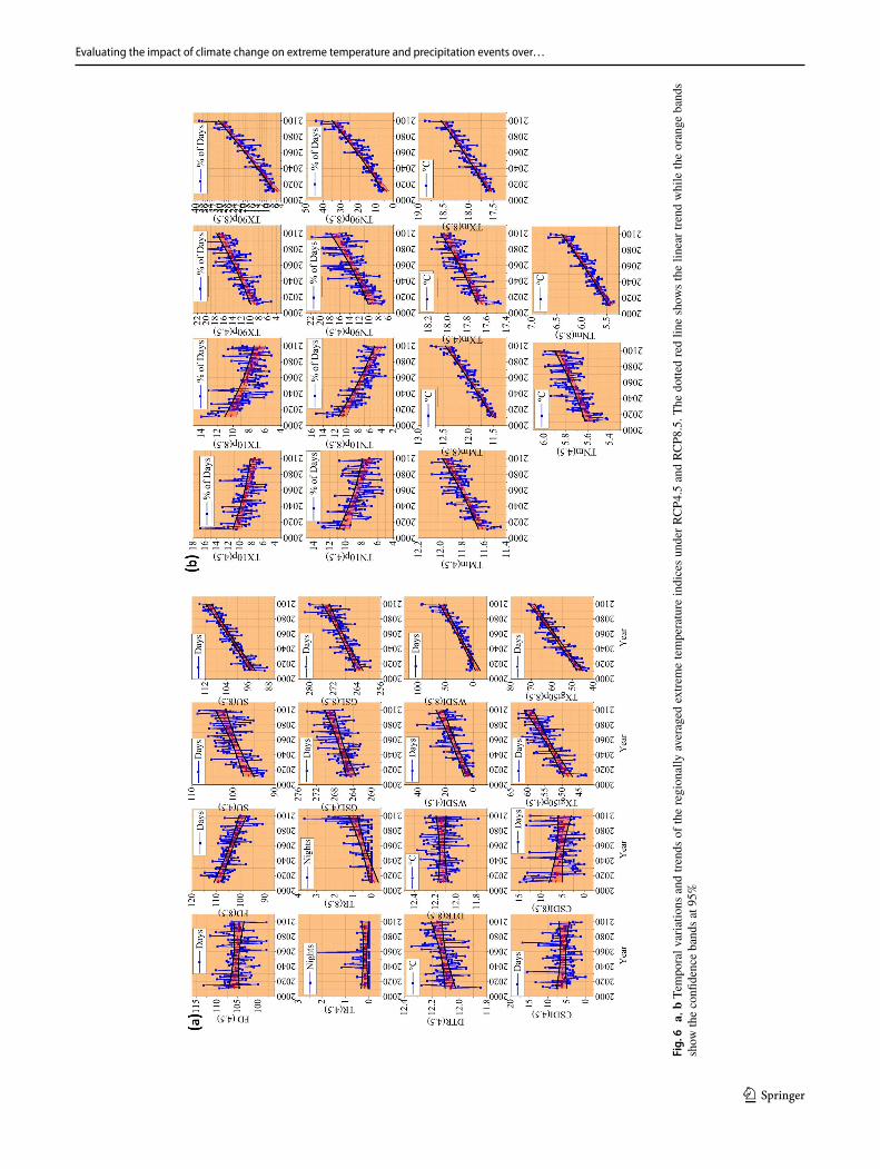
RCP8.5 for the period 2011–2100. The regional averages of the indices under RCP4.5 and RCP8.5 are shown in Figs. 6

and 7 to visualize the inter-annual variations for the period 2011–2100.

Table 1 Trend analysis of regionally averaged temperature indices under RCP4.5 and RCP8.5

Numbers in italic represent the significant trends*Significant at 0.05**Significant at 0.1

Index Time period

2020s 2050s 2080s 2011–2100

RCP4.5 RCP8.5 RCP4.5 RCP8.5 RCP4.5 RCP8.5 RCP4.5 RCP8.5

FD − 0.13** − 0.133 0.021 − 0.083 0.053 − 0.233* − 0.009 − 0.112*SU 0.138* 0.256* 0.021 0.2* 0.095 0.2* 0.082* 0.183*TR 0.00 0.00 0.00 0.00 0.00 0.024 0.00 0.005*GSL 0.023 0.111* 0.043 0.144* 0.053 0.296* 0.05* 0.122*DTR 0.00 − 0.001 0.005** 0.001 0.003 0.002 0.001* 0.00WSDI 0.108 0.144* 0.246** 0.619* − 0.033 1.5* 0.233* 0.67*CSDI − 0.103** − 0.37 − 0.022 − 0.083 − 0.111** 0.018 − 0.005 − 0.005TXgt50p 0.207** 0.382* 0.147** 0.221* 0.164** 0.188* 0.128* 0.262*TX10p − 0.071** − 0.189* − 0.046 − 0.023 − 0.064* 0.042 − 0.03* − 0.041*TX90p 0.104* 0.158* 0.1** 0.252* 0.097** 0.388* 0.085* 0.256*TN10p − 0.111* − 0.204* − 0.027 − 0.101* − 0.033 0.011* − 0.034* − 0.065*TN90p 0.132* 0.213* 0.047 0.276* 0.024 0.567* 0.089* 0.315*TMm 0.007* 0.011* 0.003 0.009* 0.004 0.014* 0.004* 0.01*TXm 0.006** 0.011** 0.006** 0.009* 0.005* 0.014** 0.004* 0.01*TNm 0.006* 0.011* 0.001 0.01* 0.002 0.015* 0.003* 0.01*

Table 2 Trend analysis of regionally averaged precipitation indices under RCP4.5 and RCP8.5

Numbers in italic represent the significant trends*Significant at 0.05**Significant at 0.1

Index Time period

2020s 2050s 2080s 2011–2100

RCP4.5 RCP8.5 RCP4.5 RCP8.5 RCP4.5 RCP8.5 RCP4.5 RCP8.5

CDD − 0.125 − 0.042 0.033 0.119 − 0.078 0.059 − 0.009 0.036**CWD 0.00 0.00 − 0.019 0.00 − 0.021 0.00 0.002 0.00PRCPTOT − 0.804 0.087 − 1.344 − 1.477 − 3.559* − 0.615 − 0.64* − 0.427**R2.5 mm − 0.042 − 0.074 − 0.077 − 0.119 − 0.115* − 0.044 − 0.018 − 0.035*R10mm 0.00 − 0.013 − 0.022 − 0.091** − 0.167* − 0.09* − 0.028* − 0.024*R20mm − 0.028 0.00 − 0.083* − 0.03 − 0.067* 0.017 − 0.011** 0.01R95p − 1.242** 0.58 − 1.175 0.566 − 0.557 0.468 − 0.339* 0.078R95ptot − 0.18* 0.055 − 0.031 0.077 0.033 0.02 − 0.015 0.015R99p − 1.177** 0.428 − 0.428 0.32 − 1.024 0.323 − 0.162 0.015R99ptot − 0.137* 0.025 − 0.034 0.046 − 0.053 0.035 − 0.014 0.001Rx1day − 0.477 0.124 − 0.077 0.109 − 0.187 0.125 − 0.066 0.06Rx5day − 0.476** 0.057 − 0.198 0.047 − 0.183 0.173 − 0.087* 0.038Rx7day − 0.513 − 0.089 − 0.141 − 0.183 − 0.47** 0.135 − 0.129* − 0.012SDII − 0.009 0.008 − 0.007 − 0.001 − 0.02** − 0.009 − 0.004* 0.001

Evaluating the impact of climate change on extreme temperature and precipitation events over…

1 3

Fig.

6 a,

b T

empo

ral v

aria

tions

and

tren

ds o

f the

regi

onal

ly a

vera

ged

extre

me

tem

pera

ture

indi

ces

unde

r RC

P4.5

and

RC

P8.5

. The

dot

ted

red

line

show

s th

e lin

ear t

rend

whi

le th

e or

ange

ban

ds

show

the

confi

denc

e ba

nds a

t 95%

S. Ahsan et al.

1 3

Fig.

7 a,

b T

empo

ral v

aria

tions

and

tren

ds o

f the

regi

onal

ly a

vera

ged

extre

me

prec

ipita

tion

indi

ces u

nder

RC

P4.5

and

RC

P8.5

. The

dot

ted

red

line

show

s the

line

ar tr

end

whi

le th

e or

ange

ban

ds

show

the

confi

denc

e ba

nds a

t 95%

Evaluating the impact of climate change on extreme temperature and precipitation events over…

1 3

5 Discussion

Changing form of the climatic extremes is important evidence and impact of anthropogenic induced climate change. In the current study, future projections of tem-perature and precipitation showed significant changes for the twenty-first century with the temperature manifesting increasing trends and precipitation showing a decrease over the basin. The present study established the imprints of global warming on the climatic extremes in the region. The model projections show increasing trends in the warm temperature-based indices while decreasing trends were found in the cold temperature-based indices for the twenty-first century. In the present study the warm extremes viz., amount of hot days/nights, fraction of days with above-average temperature, warm spell duration, summer days, and tropical nights witnessed increasing trends under RCP4.5&8.5. Consistent patterns of the trends have been reported among the different regions of the world (Klein Tank et al. 2006, 2009; Tebaldi et al. 2006; Sillmann and Roeckner 2008). A similar pattern of trends resonates over the Indian landmass and the results of the present study conform with the previous studies like Kothawale et al. (2010), Dash and Mamgain (2011), and Revadekar et al. (2012). Revadekar et al. (2012) and Mukherjee and Mishra (2018) also projected the enhancement of the hot extremes in India over the twenty-first century under different cli-mate change scenarios. While the cold extremes like the amount of cool days/nights, cold spell duration, and frost days are projected to decrease over the twenty-first century in the study area. Similar results have been reported by Gujree et al. (2017) who used the PRECIS RCM for pro-jecting the extreme climate events in the Kashmir valley.

The increase in the frequency and occurrence of the warm temperature-based extreme indices is consistent with global warming but the magnitude of change var-ies spatially due to the large-scale atmospheric circula-tion patterns associated with it (Meehl and Tebaldi 2004). Changes in the geopotential height anomalies at 500 hPa have been linked to the enhanced prevalence of the hot extremes (Ding et al. 2010; Loikith and Broccoli 2012; Lee and Lee 2016). Joshi et al. (2020) explored the physi-cal driving mechanisms responsible for the observed increases in the frequency and intensity of hot extremes over the Indian landmass. The study cited that the augmen-tation of the geopotential height anomalies at 500 hPa over the northern parts of India is leading to increases in hot extremes. The persistent atmospheric subsidence associ-ated with it results in adiabatic warming and increases atmospheric stability (Lee and Lee 2016). This phenom-enon produces clear skies and decreases in the cloud cover, thus leading to increases in hot extremes due to

pronounced surface warming. The decrease in the amount of the precipitable water is yet another mechanism yield-ing the enhancements in hot extremes over India (Joshi et al. 2020). The augmentation of temperature extremes over the twenty-first century could also be related to the inverse trends in the precipitation in the Kashmir Hima-laya. The model projections manifested a decrease in the precipitation with similar trends for the extreme precipita-tion-based indices. The length of the dry spell and the con-sequent soil moisture deficit is projected to increase in the future. The positive feedback loop induced by the reduced precipitation is causing the reduction in the soil moisture content which in turn alters the atmospheric heat fluxes. The reduced soil moisture conditions favor the decreases in latent heat flux and increases in sensible heat flux which also leads to the enhanced surface warming (Fischer et al. 2007).

Some indicators of intensification of the precipitation regimes in the region are also there e.g., the number of very heavy rainfall days, total annual precipitation from heavy and very heavy rain days, maximum 1-day precipitation, and maximum 5-day precipitation show increasing trends. Although the trends are weak but such signals cannot be ignored knowing the flood susceptibility of the region. These indices could have a direct bearing on the flood risks in the basin as the region is very prone to flood disasters. Floods have been a recurrent feature in the basin but the flood risk has increased in the recent past due to encroachment of the wetlands/waterways, urban expansion, landfilling and dis-section of the floodplain by railway/roads (Alam et al. 2018; Bhat et al. 2019). Climate change has the potential to further exacerbate the flood risks and the losses. On the other hand, the length of dry spells showing increasing trends may cause droughts in different parts of the Kashmir Himalaya. Long dry spells are an emerging concern in the study area that lead to acute water scarcity and an increase in the drought episodes (Himayoun and Roshni 2019).

6 Conclusions

Climate change will have serious implications for the mountain ecosystems like the Kashmir Himalaya. In this study, a combination of the Statistical Downscaling Model (SDSM), and ClimPACT2 were used to assess the pro-jected changes in the extreme climate (frequency and mag-nitude) over the twenty-first century. The average annual temperatures (Tmax and Tmin) have shown an increase at all the stations although with different magnitudes and patterns under the different RCPs. The projected increase varied directly with the levels of radiative forcing. The patterns of increase also revealed the orographic controls with the high altitude areas registering relatively higher

S. Ahsan et al.

1 3

increases as compared to the low altitude areas. Season-ally, autumn exhibited the highest warming followed by summer season. On the other hand, precipitation has shown a decrease in most of the area with some increases at the Gulmarg station with respect to the baseline pre-cipitation (1980–2010). Winter will be the most affected season showing significant decreases in the precipitation under all the RCPs. The projected variations in the extreme climate revealed that in response to the rising greenhouse gas concentrations in the atmosphere, the extreme climate is likely to intensify further in future. Conforming to the global trends, Kashmir Himalaya showed increasing trends in the warm temperature-based indices and a reduction in the cold extremes over the twenty-first century. The trends were more pronounced under the RCP8.5 due to higher levels of forcing and resultant warming associated with it. Precipitation indices comparatively showed divergent and spatially incoherent trends with an overall inclination towards drier regimes. The changes in the climate will have serious implications for sectors like agriculture, water resources, and human health. A decrease in the number of frost days, extensions in growing season length may be favorable for the agriculture sector but the increasing tem-peratures and decreasing precipitation will induce greater demands of water for irrigation purposes. Water resources and water dependent systems will be affected directly under the changing temperature and precipitation scenar-ios. Dry spells are a new trend of the climate in Kashmir Himalaya and recent years have marked abnormally long dry periods, creating acute water shortages. Prolonged dry spells indicated by consecutive dry days impact the surface water availability during the summer and autumn seasons. Increases in the number of hot days and nights will affect human health by increasing the thermal stresses. The results of the study can be valuable for formulating the sector-specific mitigation of climate change; how-ever, more studies are required for the analysis of climate extremes using multi-model ensembles to further refine the quantification of the changes and uncertainty associated with GCM outputs. Furthermore, increasing the density of meteorological observatories would further help in under-standing the microclimatic variation and climate change signals more lucidly.

Supplementary Information The online version contains supplemen-tary material available at https:// doi. org/ 10. 1007/ s00382- 021- 05984-6.

Acknowledgements We acknowledge the Indian Meteorological Department (IMD), Srinagar, and National Data Centre, Pune, for the providing necessary meteorological data. We would like to thank the developers of—CanESM2 GCM, Canadian Centre for Climate Model-ling and Analysis (CCCma), CFSR data, SDSM, and ClimPACT2 for keeping the data in public domain. We are indebted to the executive editor (Professor V. Krishnamurthy) and the reviewers for their insight-ful comments that improved the quality and structure of this paper.

Funding This research has been funded by University Grants Commis-sion, New Delhi, under CPEPA scheme being currently carried out at University of Kashmir, Srinagar-190006.

Open Access This article is licensed under a Creative Commons Attri-bution 4.0 International License, which permits use, sharing, adapta-tion, distribution and reproduction in any medium or format, as long as you give appropriate credit to the original author(s) and the source, provide a link to the Creative Commons licence, and indicate if changes were made. The images or other third party material in this article are included in the article's Creative Commons licence, unless indicated otherwise in a credit line to the material. If material is not included in the article's Creative Commons licence and your intended use is not permitted by statutory regulation or exceeds the permitted use, you will need to obtain permission directly from the copyright holder. To view a copy of this licence, visit http:// creat iveco mmons. org/ licen ses/ by/4. 0/.

References

Aguilar E, Auer I, Brunet M, Peterson TC, Wieringa J (2003) Guide-lines on climate metadata and homogenization. World Climate Programme Data and Monitoring WCDMP-no. 53, wmo-td no. 1186. World Meteorological Organization, Geneva, p 55

Akhtar M, Ahmad N, Booij MJ (2008) The impact of climate change on the water resources of Hindukush–Karakorum–Himalaya region under different glacier coverage scenarios. J Hydrol 355(1–4):148–163. https:// doi. org/ 10. 1016/j. jhydr ol. 2008. 03. 015

Alam A, Ahmad S, Bhat MS, Ahmad B (2015) Tectonic evolution of Kashmir basin in northwest Himalayas. Geomorphology 239:114–126. https:// doi. org/ 10. 1016/j. geomo rph. 2015. 03. 025

Alam A, Bhat MS, Kotlia BS, Ahmad B, Ahmad S, Taloor AK, Ahmad HF (2017) Coexistent pre-existing extensional and subsequent compressional tectonic deformation in the Kashmir basin, NW Himalaya. Quatern Int 444:201–208. https:// doi. org/ 10. 1016/j. quaint. 2017. 06. 009

Alam A, Bhat MS, Farooq H, Ahmad B, Ahmad S, Sheikh AH (2018) Flood risk assessment of Srinagar City in Jammu and Kashmir, India. Int J Disaster Resilience in Built Environ 9(2)114–129, https:// doi. org/ 10. 1108/ IJDRBE- 02- 2017- 0012

Alexander LV, Zhang X, Peterson TC, Caesar J, Gleason B, Klein Tank AMG et al. (2006) Global observed changes in daily climate extremes of temperature and precipitation. J Geophys Res Atmos. https:// doi. org/ 10. 1029/ 2005J D0062 90

Athar H (2014) Trends in observed extreme climate indices in Saudi Arabia during 1979–2008. Int J Climatol 34(5):1561–1574. https:// doi. org/ 10. 1002/ joc. 3783

Barnett TP, Adam JC, Lettenmaier DP (2005) Potential impacts of a warming climate on water availability in snow-dominated regions. Nature 438(7066):303–309. https:// doi. org/ 10. 1038/ natur e04141

Beniston M, Stoffel M (2014) Assessing the impacts of climatic change on mountain water resources. Sci Total Environ 493:1129–1137. https:// doi. org/ 10. 1016/j. scito tenv. 2013. 11. 122

Bhat MS, Alam A, Ahmad B, Kotlia BS, Farooq H, Taloor AK, Ahmad S (2019) Flood frequency analysis of river Jhelum in Kashmir basin. Quatern Int 507:288–294. https:// doi. org/ 10. 1016/j. quaint. 2018. 09. 039

Bradley SB, Vuille M, Diaz HF, Vergara W (2006) Threats towater supplies in the tropical Andes. Science 312:1755–1756. https:// doi. org/ 10. 1126/ scien ce. 11280 87

Campbell JL, Driscoll CT, Pourmokhtarian A, Hayhoe K (2011) Streamflow responses to past and projected future changes in cli-mate at the Hubbard Brook Experimental Forest, New Hampshire,

Evaluating the impact of climate change on extreme temperature and precipitation events over…

1 3

United States. Water Resources Res. https:// doi. org/ 10. 1029/ 2010W R0094 38

Campozano L, Sánchez E, Avilés Á, Samaniego E (2014) Evaluation of infilling methods for time series of daily precipitation and temper-ature: the case of the Ecuadorian Andes. Maskana 5(1):99–115. https:// doi. org/ 10. 18537/ mskn. 05. 01. 07

Chaturvedi RK, Joshi J, Jayaraman M, Bala G, Ravindranath NH (2012) Multi-model climate change projections for India under representative concentration pathways. Curr Sci 791–802

Chen J, Brissette FP, Leconte R (2011) Uncertainty of downscaling method in quantifying the impact of climate change on hydrol-ogy. J Hydrol 401(3–4):190–202. https:// doi. org/ 10. 1016/j. jhydr ol. 2011. 02. 020

Christensen JH, Boberg F, Christensen OB, Lucas-Picher P (2008) On the need for bias correction of regional climate change projections of temperature and precipitation. Geophys Res Lett. https:// doi. org/ 10. 1029/ 2008G L0356 94

Chu JT, Xia J, Xu CY, Singh VP (2010) Statistical downscaling of daily mean temperature, pan evaporation and precipitation for climate change scenarios in Haihe River, China. Theoret Appl Climatol 99(1–2):149–161. https:// doi. org/ 10. 1007/ s00704- 009- 0129-6

Coulibaly P, Dibike YB, Anctil F (2005) Downscaling precipitation and temperature with temporal neural networks. J Hydrometeorol 6(4):483–496. https:// doi. org/ 10. 1175/ JHM409.1

Dash SK, Mamgain A (2011) Changes in the frequency of different categories of temperature extremes in India. J Appl Meteorol Cli-matol 50(9):1842–1858

Dibike YB, Coulibaly P (2005) Hydrologic Impact of Climate Change in the Saguenay Watershed: Comparison of Downscaling Methods and Hydrologic Models. J Hydrol 307:145–163. https:// doi. org/ 10. 1016/j. jhydr ol. 2004. 10. 012

Dile YT, Srinivasan R (2014) Evaluation of CFSR climate data for hydrologic prediction in data-scarce watersheds: an application in the Blue Nile River Basin. JAWRA J Am Water Resources Assoc 50(5):1226–1241. https:// doi. org/ 10. 1111/ jawr. 12182

Dimri AP, Dash SK (2012) Wintertime climatic trends in the western Himalayas. Clim Change 111(3–4):775–800

Ding T, Qian W, Yan Z (2010) Changes in hot days and heat waves in China during 1961–2007. Int J Climatol 30(10):1452–1462

Donat MG, Alexander LV, Yang H, Durre I, Vose R, Dunn RJH et al (2013) Updated analyses of temperature and precipitation extreme indices since the beginning of the twentieth century: The HadEX2 dataset. J Geophys Res Atmos 118(5):2098–2118

Easterling DR, Meehl GA, Parmesan C, Changnon SA, Karl TR, Mearns LO (2000) Climate extremes: observations, modeling, and impacts. Science 289(5487):2068–2074. https:// doi. org/ 10. 1126/ scien ce. 289. 5487. 2068

Fang G, Yang J, Chen YN, Zammit C (2015) Comparing bias cor-rection methods in downscaling meteorological variables for a hydrologic impact study in an arid area in China. Hydrol Earth Syst Sci 19(6):2547–2559

Fischer EM, Seneviratne SI, Vidale PL, Lüthi D, Schär C (2007) Soil moisture–atmosphere interactions during the 2003 European sum-mer heat wave. J Clim 20(20):5081–5099

Fischer EM, Beyerle U, Knutti R (2013) Robust spatially aggregated projections of climate extremes. Nat Clim Chang 3(12):1033–1038. https:// doi. org/ 10. 1038/ nclim ate20 51

Fowler HJ, Blenkinsop S, Tebaldi C (2007) Linking climate change modelling to impacts studies: recent advances in downscaling techniques for hydrological modelling. Int J Climatol J R Meteorol Soc 27(12):1547–1578. https:// doi. org/ 10. 1002/ joc. 1556

Fuka DR, Walter MT, MacAlister C, Degaetano AT, Steenhuis TS, Easton ZM (2014) Using the Climate Forecast System Reanaly-sis as weather input data for watershed models. Hydrol Process 28(22):5613–5623

Gagnon S, Singh B, Rousselle J, Roy L (2005) An application of the statistical downscaling model (SDSM) to simulate climatic data for streamflow modelling in Québec. Can Water Resources J 30(4):297–314

Gan R, Luo Y, Zuo Q, Sun L (2015) Effects of projected climate change on the glacier and runoff generation in the Naryn River Basin, Central Asia. J Hydrol 523:240–251. https:// doi. org/ 10. 1016/j. jhydr ol. 2015. 01. 057

Gujree I, Wani I, Muslim M, Farooq M, Meraj G (2017) Evaluating the variability and trends in extreme climate events in the Kashmir Valley using PRECIS RCM simulations. Model Earth Syst Envi-ron 3(4):1647–1662. https:// doi. org/ 10. 1007/ s40808- 017- 0370-4

Hashmi MZ, Shamseldin AY, Melville BW (2010) Comparison of SDSM and LARS-WG for simulation and downscaling of extreme precipitation events in a watershed. Stoch Environ Res Risk Assess. https:// doi. org/ 10. 1007/ s00477- 010- 0416-x

Hay LE, Clark MP (2003) Use of statistically and dynamically down-scaled atmospheric model output for hydrologic simulations in three mountainous basins in the western United States. J Hydrol 282(1–4):56–75. https:// doi. org/ 10. 1016/ s0022- 1694(03) 00252-x

Himayoun D, Roshni T (2019) Spatio-temporal variation of drought characteristics, water resource availability and the relation of drought with large scale climate indices: a case study of Jhelum basin, India. Quatern Int 525:140–150

Huang J, Zhang J, Zhang Z, Xu C, Wang B, Yao J (2011) Estimation of future precipitation change in the Yangtze River basin by using statistical downscaling method. Stoch Environ Res Risk Assess 25(6):781–792. https:// doi. org/ 10. 1007/ s00477- 010- 0441-9

Huang J, Zhang J, Zhang Z, Sun S, Yao J (2012) Simulation of extreme precipitation indices in the Yangtze River basin by using statisti-cal downscaling method (SDSM). Theoret Appl Climatol 108(3–4):325–343. https:// doi. org/ 10. 1007/ s00704- 011- 0536-3

Huang YF, Ang JT, Tiong YJ, Mirzaei M, Amin MZM (2016) Drought forecasting using SPI and EDI under RCP-8.5 climate change sce-narios for Langat River Basin, Malaysia. Procedia Eng 154:710–717. https:// doi. org/ 10. 1016/j. proeng. 2016. 07. 573

Husain M (1987) Geography of Jammu & Kashmir State. Rejesh Pub-lications, New Delhi

Immerzeel WW, Van Beek LP, Bierkens MF (2010) Climate change will affect the Asian water towers. Science 328(5984):1382–1385. https:// doi. org/ 10. 1126/ scien ce. 118318

Ines AV, Hansen JW (2006) Bias correction of daily GCM rainfall for crop simulation studies. Agric Meteorol 138(1–4):44–53

Joshi MK, Rai A, Kulkarni A, Kucharski F (2020) Assessing changes in characteristics of hot extremes over India in a warming environ-ment and their driving mechanisms. Sci Rep 10(1):1–14

Khadka D, Pathak D (2016) Climate change projection for the marsy-angdi river basin, Nepal using statistical downscaling of GCM and its implications in geodisasters. Geoenviron Disasters 3(1):15. https:// doi. org/ 10. 1186/ s40677- 016- 0050-0

Khan MS, Coulibaly P, Dibike Y (2006) Uncertainty analysis of statis-tical downscaling methods. J Hydrol 319(1–4):357–382. https:// doi. org/ 10. 1016/j. jhydr ol. 2005. 06. 035

Kharin VV, Zwiers FW, Zhang X, Wehner M (2013) Changes in tem-perature and precipitation extremes in the CMIP5 ensemble. Clim Change 119(2):345–357. https:// doi. org/ 10. 1175/ JCLI4 066.1

Klein Tank AMG, Peterson TC, Quadir DA, Dorji S, Zou X, Tang H et al (2006) Changes in daily temperature and precipitation extremes in Central and South Asia. J Geophys Res Atmos. https:// doi. org/ 10. 1007/ s00477- 012- 0615-8

Klein Tank AMG, Zwiers FW, Zhang X (2009) Guidelines on analysis of extremes in a changing climate in support of informed deci-sions for adaptation. Climate data and monitoring WCDMP-No. 72, WMO-TD No. 1500, pp 56

S. Ahsan et al.

1 3

Kostopoulou E, Jones PD (2005) Assessment of climate extremes in the Eastern Mediterranean. Meteorol Atmos Phys 89(1–4):69–85. https:// doi. org/ 10. 1007/ s00703- 005- 0122-2

Kothawale DR, Revadekar JV, Kumar KR (2010) Recent trends in pre-monsoon daily temperature extremes over India. J Earth Syst Sci 119(1):51–65

Koukidis EN, Berg AA (2009) Sensitivity of the Statistical Down-Scaling Model (SDSM) to reanalysis products. Atmos Ocean 47(1):1–18. https:// doi. org/ 10. 3137/ AO924. 2009

Lee WS, Lee MI (2016) Interannual variability of heat waves in South Korea and their connection with large-scale atmospheric circula-tion patterns. Int J Climatol 36(15):4815–4830

Lenderink G, Buishand A, Van Deursen W (2007) Estimates of future discharges of the river Rhine using two scenario meth-odologies: direct versus delta approach

Liu LL, Liu ZF, Xu ZX (2008) Trends of climate change for the upper-middle reaches of the Yellow River in the 21st century. Adv Clim Chang Res 4(3):167–172

Loikith PC, Broccoli AJ (2012) Characteristics of observed atmos-pheric circulation patterns associated with temperature extremes over North America. J Clim 25(20):7266–7281

Mahmood R, Babel MS (2013) Evaluation of SDSM developed by annual and monthly sub-models for downscaling temperature and precipitation in the Jhelum basin, Pakistan and India. Theo-ret Appl Climatol 113(1–2):27–44

Mahmood R, Babel MS (2014) Future changes in extreme tempera-ture events using the statistical downscaling model (SDSM) in the trans-boundary region of the Jhelum river basin. Weather Clim Extremes 5:56–66. https:// doi. org/ 10. 1016/j. wace. 2014. 09. 001

Mahmood R, Babel MS, Shaofeng JIA (2015) Assessment of temporal and spatial changes of future climate in the Jhelum river basin, Pakistan and India. Weather Clim Extremes 10:40–55. https:// doi. org/ 10. 1016/j. wace. 2015. 07. 002

Mearns LO, Giorgi F, Whetton P, Pabon D, Hulme M, Lal M (2003) Guidelines for use of climate scenarios developed from regional climate model experiments

Meehl GA, Tebaldi C (2004) More intense, more frequent, and longer lasting heat waves in the 21st century. Science 305(5686):994–997

Meenu R, Rehana S, Mujumdar PP (2013) Assessment of hydrologic impacts of climate change in Tunga-Bhadra river basin, India with HEC-HMS and SDSM. Hydrol Process 27(11):1572–1589. https:// doi. org/ 10. 16943/ ptinsa/ 2018/ 49506

Morak S, Hegerl GC, Christidis N (2013) Detectable changes in the fre-quency of temperature extremes. J Clim 26(5):1561–1574. https:// doi. org/ 10. 1175/ JCLI-D- 11- 00678.1

Mukherjee S, Mishra V (2018) A sixfold rise in concurrent day and night-time heatwaves in India under 2 C warming. Sci Rep 8(1):1–9

Nguyen VTV, Nguyen TD, Gachon P (2006) On the linkage of large-scale climate variability with local characteristics of daily pre-cipitation and temperature extremes: an evaluation of statistical downscaling methods. Adv Geosci Hydrol Sci (HS) 4:1–9. https:// doi. org/ 10. 1142/ 97898 12707 208_ 0001

Nguyen VTV, Nguyen TD, Cung A (2007) A statistical approach to downscaling of sub-daily extreme rainfall processes for climate-related impact studies in urban areas. Water Sci Technol Water Supply 7(2):183–192. https:// doi. org/ 10. 2166/ ws. 2007. 053

Orlowsky B, Seneviratne SI (2012) Global changes in extreme events: regional and seasonal dimension. Clim Change 110(3–4):669–696. https:// doi. org/ 10. 1007/ s10584- 011- 0122-9

Otto FE, Massey N, Van Oldenborgh GJ, Jones RG, Allen MR (2012) Reconciling two approaches to attribution of the 2010 Russian heat wave. Geophys Res Lett. https:// doi. org/ 10. 1029/ 2011G L0504 22

Rashid I, Romshoo SA, Chaturvedi RK, Ravindranath NH, Sukumar R, Jayaraman M et al (2015) Projected climate change impacts on vegetation distribution over Kashmir Himalayas. Clim Change 132(4):601–613. https:// doi. org/ 10. 1007/ s10584- 015- 1456-5

Revadekar JV, Kothawale DR, Patwardhan SK, Pant GB, Kumar KR (2012) About the observed and future changes in temperature extremes over India. Nat Hazards 60(3):1133–1155

Roy S, Balling RC Jr (2004) Trends in extreme daily precipitation indices in India. Int J Climatol J R Meteorol Soc 24(4):457–466. https:// doi. org/ 10. 1002/ joc. 995

Saha S, Moorthi S, Pan HL, Wu X, Wang J, Nadiga S et al (2010) The NCEP climate forecast system reanalysis. Bull Am Meteor Soc 91(8):1015–1058. https:// doi. org/ 10. 1175/ 2010B AMS30 01.1

Samadi S, Wilson CA, Moradkhani H (2013) Uncertainty analysis of statistical downscaling models using Hadley Centre Coupled Model. Theoret Appl Climatol 114(3–4):673–690. https:// doi. org/ 10. 1007/ s00704- 013- 0844-x

Sen PK (1968) Estimates of the regression coefficient based on Kend-all’s tau. J Am Stat Assoc 63(324):1379–1389

Shafiq M, Ramzan S, Ahmed P, Mahmood R, Dimri AP (2019) Assess-ment of present and future climate change over Kashmir Himala-yas, India. Theoret Appl Climatol 137(3–4):3183–3195. https:// doi. org/ 10. 1007/ s00704- 019- 02807-x

Sharma KP, Vorosmarty CJ, Moore B (2000) Sensitivity of the Hima-layan hydrology to land-use and climatic changes. Clim Change 47(1–2):117–139

Sharma E, Molden D, Wester P, Shrestha RM (2016) The Hindu Kush Himalayan monitoring and assessment programme: action to sus-tain a global asset. Mt Res Dev 36(2):236–239. https:// doi. org/ 10. 1659/ MRD- JOURN AL-D- 16- 00061.1

Shekhar MS, Devi U, Paul S, Singh GP, Singh A (2017) Analysis of trends in extreme precipitation events over Western Himalaya Region: intensity and duration wise study. J Ind Geophys Union 21(3):225–231

Sillmann J, Roeckner E (2008) Indices for extreme events in projections of anthropogenic climate change. Clim Change 86(1–2):83–104. https:// doi. org/ 10. 1007/ s10584- 007- 9308-6

Sillmann J, Kharin VV, Zwiers FW, Zhang X, Bronaugh D (2013) Cli-mate extremes indices in the CMIP5 multimodel ensemble: Part 2. Future climate projections. J Geophys Res Atmos 118(6):2473–2493. https:// doi. org/ 10. 1002/ jgrd. 50188

Souvignet M, Heinrich J (2011) Statistical downscaling in the arid central Andes: uncertainty analysis of multi-model simu-lated temperature and precipitation. https:// doi. org/ 10. 1007/ s00704- 011- 0430-z

Tabari H, Somee BS, Zadeh MR (2011) Testing for long-term trends in climatic variables in Iran. Atmos Res 100(1):132–140. https:// doi. org/ 10. 1016/j. atmos res. 2011. 01. 005

Tebaldi C, Hayhoe K, Arblaster JM, Meehl GA (2006) Going to the extremes. Clim Change 79(3–4):185–211. https:// doi. org/ 10. 1007/ s10584- 006- 9051-4

Teutschbein C, Seibert J (2010) Regional climate models for hydro-logical impact studies at the catchment scale: a review of recent modeling strategies. Geogr Compass 4(7):834–860

Teutschbein C, Wetterhall F, Seibert J (2011) Evaluation of different downscaling techniques for hydrological climate-change impact studies at the catchment scale. Clim Dyn 37(9–10):2087–2105. https:// doi. org/ 10. 1007/ s00382- 010- 0979-8

Trenberth KE (2011) Attribution of climate variations and trends to human influences and natural variability. Wiley Interdiscip Rev Clim Change 2(6):925–930. https:// doi. org/ 10. 1002/ wcc. 142

Turco M, Sanna A, Herrera S, Llasat MC, Gutiérrez JM (2013) Large biases and inconsistent climate change signals in ENSEMBLES regional projections. Clim Change 120(4):859–869. https:// doi. org/ 10. 1007/ s10584- 013- 0844-y

Evaluating the impact of climate change on extreme temperature and precipitation events over…

1 3

Van Vuuren DP, Edmonds J, Kainuma M, Riahi K, Thomson A, Hib-bard K et al (2011) The representative concentration pathways: an overview. Clim Change 109(1–2):5. https:// doi. org/ 10. 1007/ s10584- 011- 0148-z

Varis O, Kajander T, Lemmelä R (2004) Climate and water: from cli-mate models to water resources management and vice versa. Clim Change 66(3):321–344. https:// doi. org/ 10. 1023/B: CLIM. 00000 44622. 42657. d4

Vincent LA, Zhang X, Mekis É, Wan H, Bush EJ (2018) Changes in Canada’s climate: trends in indices based on daily temperature and precipitation data. Atmos Ocean 56(5):332–349. https:// doi. org/ 10. 1080/ 07055 900. 2018. 15145 79

Von Salzen K, Scinocca JF, McFarlane NA, Li J, Cole JN, Plummer D et al (2013) The Canadian fourth generation atmospheric global climate model (CanAM4). Part I: representation of physical pro-cesses. Atmos Ocean 51(1):104–125. https:// doi. org/ 10. 1080/ 07055 900. 2012. 755610

Wilby RL, Dawson CW (2007) SDSM 4.2—a decision support tool for the assessment of regional climate change impacts, Version 4.2 User Manual. Lancaster University, Lancaster/Environment Agency of England and Wales, Lancaster, pp 1–94

Wilby RL, Wigley TML (1997) Downscaling general circulation model output: a review of methods and limitations. Prog Phys Geogr 21(4):530–548. https:// doi. org/ 10. 1177/ 03091 33397 02100 403

Wilby RL, Dawson CW, Barrow EM (2002) SDSM—a decision sup-port tool for the assessment of regional climate change impacts. Environ Model Softw 17(2):145–157. https:// doi. org/ 10. 1016/ S1364- 8152(01) 00060-3

Yao T, Thompson LG, Mosbrugger V, Zhang F, Ma Y, Luo T et al (2012) Third pole environment (TPE). Environ Dev 3:52–64. https:// doi. org/ 10. 1016/j. envdev. 2012. 04. 002

Zhan YJ, Ren GY, Shrestha AB, Rajbhandari R, Ren YY, Sanjay J et al (2017) Changes in extreme precipitation events over the Hindu Kush Himalayan region during 1961–2012. Adv Clim Chang Res 8(3):166–175

Zhang X, Aguilar E, Sensoy S, Melkonyan H, Tagiyeva U, Ahmed N et al (2005) Trends in Middle East climate extreme indices from 1950 to 2003. J Geophys Res Atmos. https:// doi. org/ 10. 1029/ 2005J D0061 81

Zhang X, Alexander L, Hegerl GC, Jones P, Tank AK, Peterson TC, Zwiers FW (2011) Indices for monitoring changes in extremes based on daily temperature and precipitation data. Wiley Inter-discip Rev Clim Change 2(6):851–870

Zhu X, Zhang A, Wu P, Qi W, Fu G, Yue G, Liu X (2019) Uncertainty impacts of climate change and downscaling methods on future runoff projections in the Biliu River Basin. Water 11(10):2130. https:// doi. org/ 10. 3390/ w1110 2130

Publisher's Note Springer Nature remains neutral with regard to jurisdictional claims in published maps and institutional affiliations.