Economic Research Southern Africa (ERSA) is a research programme funded by the National

Treasury of South Africa. The views expressed are those of the author(s) and do not necessarily represent those of the funder, ERSA or the author’s affiliated

institution(s). ERSA shall not be liable to any person for inaccurate information or opinions contained herein.

Evaluating South Africa’s Tobacco Control

Initative: A Synthetic Control Approach

Grieve Chelwa, Corné van Walbeek and Evan Blecher

ERSA working paper 567

December 2015

Evaluating South Africa’s Tobacco ControlInitiative: A Synthetic Control Approach

Grieve Chelwa¤, Corné van Walbeekyand Evan Blecherz

December 9, 2015

Abstract

South Africa has since 1994 consistently and aggressively increasedexcise taxes on cigarettes in order to maintain a total tax burden of around50% of the average retail selling price. The tax rises have translated intolarge increases in the in‡ation-adjusted price of cigarettes. For instance,the average real price per pack increased by 110% between 1994 and 2004.This paper uses a transparent and data-driven technique, the SyntheticControl method, to evaluate the impact on cigarette consumption of SouthAfrica’s large-scale tobacco tax increases. We …nd that per capita cigaretteconsumption would not have continued declining in the absence of theconsistent tax rises that began in 1994. Speci…cally, we …nd that by 2004,per capita cigarette consumption was 36% lower than it would have beenhad the tax increases not occurred. Our treatment e¤ect estimates survivea series of placebo and robustness tests.

1 Introduction

South Africa has since 1994 aggressively and consistently increased the excisetax on cigarettes so as to meet and maintain a total tax burden (including ValueAdded Tax) of 50% of the average retail selling price. The target was met in1997 and revised upwards to 52% in 2004. The tax rises have translated intosubstantial increases in the in‡ation-adjusted retail selling prices of cigarettes.For instance, the average real price per pack of cigarettes increased by 110%between 1994 and 2004 and by 190% if one extends the period to 2012 (see Figure1). The increase in prices has coincided with substantial declines in prevalenceand consumption. Van Walbeek (2005) estimated that prevalence declined from31% of the adult population in 1993 to 24% in 2003 while aggregate cigarette

¤School of Economics, University of Cape Town, Cape Town, South Africa. Email: griev-echelwa@gmail.com.

ySchool of Economics, University of Cape Town, Cape Town, South Africa. Email: cwal-beek@gmail.com.

zWorld Health Organization and A¢liate, Economics of Tobacco Control Project, Univer-sity of Cape Town. Email: blechere@who.int.

1

consumption and per capita consumption declined by 32% and 46% respectivelyover the same period.

Declines in prevalence and consumption were well underway by the timethe tax increases began in 1994 (Van Walbeek, 2002; 2005). In the absence of acredible counterfactual (a what-if scenario), the impact of taxes on consumptionand prevalence is likely to be overstated. The literature on evaluating the impactof South Africa’s aggressive tobacco control e¤orts is not very extensive.

This paper uses a transparent data-driven technique, the Synthetic Controlmethod developed by Abadie and Gardeazabal (2003) and extended in Abadie etal. (2010), to create a credible counterfactual of cigarette consumption in SouthAfrica from 1994 to 2004. The counterfactual is constructed as a weightedaverage of the per capita cigarette consumption of countries similar to SouthAfrica that did not initiate large-scale tobacco control measures over the period1994 to 2004. Using this counterfactual, we are able to estimate a “treatmente¤ect” of South Africa’s tax increases on cigarette consumption. We …nd thatper capita cigarette consumption would not have continued declining in theabsence of the consistent tax and price rises that began in 1994. Speci…cally,we estimate a treatment e¤ect of 36% by 2004. That is, per capita cigaretteconsumption in 2004 was 36% lower than it would have been had the governmentnot consistently increased excise taxes in the preceding years.

The rest of this paper is structured as follows: Section 2 provides somebackground to South Africa’s tobacco control measures. Section 3 reviews theliterature evaluating tobacco control measures in South Africa and in other partsof the world. Section 4 describes the Synthetic Control method in some detailand Section 5 describes the data. Section 6 discusses the selection of the controlcountries (what we call the donor pool) while Section 7 presents the main resultsand conducts placebo tests. We present the results of the robustness tests inSection 8 while Section 9 discusses what implications, if any, illicit trade has formy estimates of the treatment e¤ect. Section 10 concludes.

2 Tobacco Control in South AfricaPrior to 1994, South Africa did not consciously target the consumption of to-bacco products on public health grounds. According to Van Walbeek (2005), therelegation of public health concerns in tobacco tax policy was likely due to thecordial relations that existed between the tobacco industry and the NationalParty, the party that ruled South Africa from 1948 to 1994. The end resultwas that the real tax on cigarettes, the main tobacco product in South Africa,declined by 70% between 1961 and 1990 (ibid.). Coincidentally, per capita ciga-rette consumption increased by 60% from 50 packs in 1961 to 80 packs in 1991(ibid.).

In the 1980s and early 1990s, the medical research community (Yach, 1982)and the South African Medical Research Council (1988, 1992) published re-search showing that tobacco consumption imposed a net cost on the country.For instance, the 1992 study by the South African Medical Research Council

2

(SAMRC) estimated the costs of tobacco consumption at 1.82% of GDP againstbene…ts of 0.49% of GDP (SAMRC, 1992). The publicity generated by thesestudies rallied the public health community and civil society behind the commongoal of getting the South African government to take tobacco control seriously.The momentum that had built up during the 1980s and early 1990s, along withthe impending change of government, culminated in the passing of the TobaccoProducts Control Act of 1993 by Parliament.1 The big turning point, how-ever, came in 1994 when the new African National Congress-led governmentannounced that the government would target a tax burden on cigarettes (in-cluding Value Added Tax) of 50% of the retail price to be phased in over anumber of years (Republic of South Africa, 1994). As a result, 1994, 1995 and1996 saw excise tax increments of respectively 25%, 25% and 18% (Republic ofSouth Africa, 1994, 1995, 1996). In 1997, the Minister of Finance announced alarge increase of 52% in the excise tax on cigarettes, a move that was expectedto bring the total tax burden (including Value Added Tax) to 50% of the aver-age retail selling price (Republic of South Africa, 1997). From 1997, the annualincreases on excise taxes on cigarettes have, therefore, been predictable in or-der to maintain the stipulated tax burden.2 In 2004, the total tax burden wasrevised upwards to 52% of the average retail selling price (Republic of SouthAfrica, 2004).

South Africa’s aggressive excise tax policy since 1994 has translated intosubstantial increases in the real price of cigarettes (see Figure 1). From 1994 to2012, the average real price per pack of cigarettes increased by 190%. Between1994 and 2004, which is the period we evaluate in this paper, the increase inthe real price per pack was 110%. This is in stark contrast to the period before1994 which saw considerable declines in the real excise tax on cigarettes and inthe real price of cigarettes. It is this unprecedented increase in real cigaretteprices, beginning in 1994, whose impact on consumption we seek to evaluate inthis paper.

3 Literature reviewThe literature evaluating the impact of South Africa’s tax increases since 1994on prevalence and consumption is not very extensive. Van Walbeek (2002, 2005)investigated the impact of the tax increases on prevalence and consumption by…tting a linear trend to the All Media and Products Survey (AMPS), whichis a commercially generated dataset. He estimated that smoking prevalencein South Africa declined from 31% of the adult population in 1993 to 24% in2003. He also found that African and Coloured population groups experiencedthe biggest declines in prevalence over the same period. In terms of consump-

1Saloojee (1994), Malan and Leaver (2003) and Van Walbeek (2005) contain detailed ac-counts of the events and debates leading up to the adoption of the Tobacco Products ControlAct of 1993.

2Because the industry responds by increasing retail prices, the tax burden is always slightlyless than the government’s target (see Van Walbeek, 2005, 2006).

3

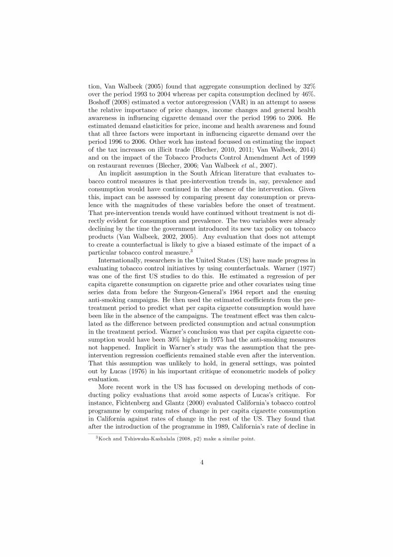
tion, Van Walbeek (2005) found that aggregate consumption declined by 32%over the period 1993 to 2004 whereas per capita consumption declined by 46%.Bosho¤ (2008) estimated a vector autoregression (VAR) in an attempt to assessthe relative importance of price changes, income changes and general healthawareness in in‡uencing cigarette demand over the period 1996 to 2006. Heestimated demand elasticities for price, income and health awareness and foundthat all three factors were important in in‡uencing cigarette demand over theperiod 1996 to 2006. Other work has instead focussed on estimating the impactof the tax increases on illicit trade (Blecher, 2010, 2011; Van Walbeek, 2014)and on the impact of the Tobacco Products Control Amendment Act of 1999on restaurant revenues (Blecher, 2006; Van Walbeek et al., 2007).

An implicit assumption in the South African literature that evaluates to-bacco control measures is that pre-intervention trends in, say, prevalence andconsumption would have continued in the absence of the intervention. Giventhis, impact can be assessed by comparing present day consumption or preva-lence with the magnitudes of these variables before the onset of treatment.That pre-intervention trends would have continued without treatment is not di-rectly evident for consumption and prevalence. The two variables were alreadydeclining by the time the government introduced its new tax policy on tobaccoproducts (Van Walbeek, 2002, 2005). Any evaluation that does not attemptto create a counterfactual is likely to give a biased estimate of the impact of aparticular tobacco control measure.3

Internationally, researchers in the United States (US) have made progress inevaluating tobacco control initiatives by using counterfactuals. Warner (1977)was one of the …rst US studies to do this. He estimated a regression of percapita cigarette consumption on cigarette price and other covariates using timeseries data from before the Surgeon-General’s 1964 report and the ensuinganti-smoking campaigns. He then used the estimated coe¢cients from the pre-treatment period to predict what per capita cigarette consumption would havebeen like in the absence of the campaigns. The treatment e¤ect was then calcu-lated as the di¤erence between predicted consumption and actual consumptionin the treatment period. Warner’s conclusion was that per capita cigarette con-sumption would have been 30% higher in 1975 had the anti-smoking measuresnot happened. Implicit in Warner’s study was the assumption that the pre-intervention regression coe¢cients remained stable even after the intervention.That this assumption was unlikely to hold, in general settings, was pointedout by Lucas (1976) in his important critique of econometric models of policyevaluation.

More recent work in the US has focussed on developing methods of con-ducting policy evaluations that avoid some aspects of Lucas’s critique. Forinstance, Fichtenberg and Glantz (2000) evaluated California’s tobacco controlprogramme by comparing rates of change in per capita cigarette consumptionin California against rates of change in the rest of the US. They found thatafter the introduction of the programme in 1989, California’s rate of decline in

3Koch and Tshiswaka-Kashalala (2008, p2) make a similar point.

4

per capita cigarette consumption exceeded that of the rest of the US by 2.72packs per year. A critique of the method in Fichtenberg and Glantz (2000) isthat treatment e¤ects were underestimated since the rest of the US includedstates that, alongside California, had also implemented some tobacco controlmeasures.4 The method in Abadie et al. (2010), which we describe fully below,attempts to correct for this shortcoming by comparing California to only thosestates that did not implement large-scale tobacco control measures after 1989.

4 Method

This paper uses the method developed by Abadie and Gardeazabal (2003) andextended further in Abadie et al. (2010) to evaluate South Africa’s tobacco con-trol policies from 1994 to 2004. The method involves estimating South Africa’scounterfactual cigarette consumption trend line following the consistent hikes incigarette excise taxes that began in 1994. In other words, the method involvescreating a synthetic South Africa, a country that looks like South Africa in allrelevant respects except for the tax hikes. The observed outcome variable forthe “real” South Africa is then compared to the outcome variable for the syn-thetic South Africa. In this section we discuss in some detail the formal aspectsof the method.

4.1 Identi…cation

Suppose we have J + 1 regions and region 1 experiences a policy change andis therefore referred to as the “treated” region. The remaining J regions donot experience the policy change and since we use these regions to constructa counterfactual scenario for the treated country, we collectively refer to themas the “donor” pool. The policy change happens at time period T0 where 1 ·T0 < T0 + P with P being the number of time periods after treatment. In thecase of South Africa, P = 10 and T0 = 1994 (Below we motivate why we chooseto end the evaluation 10 years after 1994). The outcome variable of interest isYit with i = 1, 2, ..., J +1 and t = 1, ..., T0 +P. For any region i and time periodt, we can de…ne Y I

it and Y Nit .Y I

it is the observed outcome variable and Y Nit is

the outcome variable in the absence of treatment (the superscripts I and N arechosen to represent respectively “intervention” and “no intervention”). That is,Y N

it is unobserved after T0 but is equal to Y Iit before T0. Given this, we can then

de…ne the treatment e¤ect of the policy change, αit,as:

αit = Y Iit ¡ Y N

it (1)

for t = T0 +1, . . . , T0 +P. The complication is that Y Nit is unobserved for all

t > T0.. In order to estimate the e¤ect of the policy change, we need to estimateY N

it after treatment. Suppose Yit evolves according to the equation

4For example, Alaska, Hawaii, Maryland, Michigan, New Jersey, New York and Washingtonhad raised their state cigarette taxes by at least 50 US cents over the period 1989 to 2000(Abadie et al., 2010).

5

Yit = λt + µtZi + ±t¹i + εit (2)

where λt is some factor common to all regions, Zi is a vector of observedfactors and ¹i is a vector of unobserved factors that have an impact on Yit.µt and δt are the unknown time varying parameters associated with Zi and ¹i

respectively5. εit is the unobserved error term with mean zero. Given a donorpool and a J £ 1 vector of weights W = (w2, . . . , wj+1)

0 such that wj ¸ 0 andw2 + w3 + ¢ ¢ ¢ + wj+1 = 1, we can construct for any i

J+1Xj=2

wjYjt = λt + µt

J+1Xj=2

wjZj + ±t

J+1Xj=2

wj¹j +J+1Xj=2

wjεit (3)

That is, we can always express the outcome variable of a treated regionas a weighted average of the regions in the donor pool. For i = 1 (i.e. thetreated country), Abadie and Gardeazabal (2003) and Abadie et al. (2010)show that there exists a J £ 1 vector of weights W¤ = (w¤

2, . . . , w¤J+1)

0 withw¤

2 + w¤3 + . . . w¤

J+1 = 1 and w¤j ¸ 0 such that

J+1Xj=2

w¤j Yj1 = Y11 (4)

J+1Xj=2

w¤j Yj2 = Y12

.

.

.

J+1Xj=2

w¤j YjT0 = Y1T0 and

J+1Xj=2

w¤j Zj = Z1

That is, we can exactly recreate the pre-treatment characteristics of thetreated region using only the donor pool and the weights in W¤6 . Since thefactors in ¹i are unobserved, we cannot create their empirical counterparts inequation (4). However, if the set of equations in (4) hold exactly, then

5Notice that Zi and µi do not have time subscripts. We can think of their values as …xedover short periods of time but still allow for their e¤ects, via θt and δt respectively, to varyacross time. The method also allows for more general speci…cations of Zi and µ with timesubscripts.

6Appendix B of Abadie et al. (2010) contains the mathematical proofs related to thispoint.

6

J+1Xj=2

w¤j ¹i = ¹1 (5)

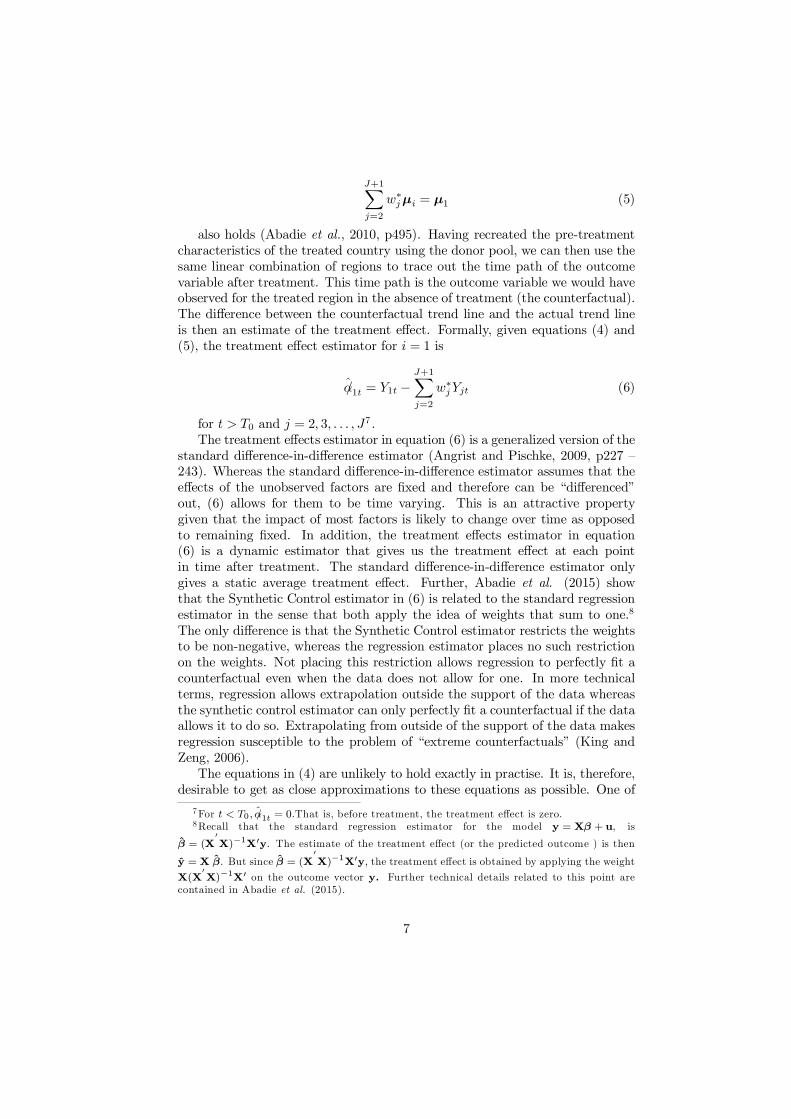
also holds (Abadie et al., 2010, p495). Having recreated the pre-treatmentcharacteristics of the treated country using the donor pool, we can then use thesame linear combination of regions to trace out the time path of the outcomevariable after treatment. This time path is the outcome variable we would haveobserved for the treated region in the absence of treatment (the counterfactual).The di¤erence between the counterfactual trend line and the actual trend lineis then an estimate of the treatment e¤ect. Formally, given equations (4) and(5), the treatment e¤ect estimator for i = 1 is

/α1t = Y1t ¡J+1Xj=2

w¤j Yjt (6)

for t > T0 and j = 2, 3, . . . , J7 .The treatment e¤ects estimator in equation (6) is a generalized version of the

standard di¤erence-in-di¤erence estimator (Angrist and Pischke, 2009, p227 –243). Whereas the standard di¤erence-in-di¤erence estimator assumes that thee¤ects of the unobserved factors are …xed and therefore can be “di¤erenced”out, (6) allows for them to be time varying. This is an attractive propertygiven that the impact of most factors is likely to change over time as opposedto remaining …xed. In addition, the treatment e¤ects estimator in equation(6) is a dynamic estimator that gives us the treatment e¤ect at each pointin time after treatment. The standard di¤erence-in-di¤erence estimator onlygives a static average treatment e¤ect. Further, Abadie et al. (2015) showthat the Synthetic Control estimator in (6) is related to the standard regressionestimator in the sense that both apply the idea of weights that sum to one.8

The only di¤erence is that the Synthetic Control estimator restricts the weightsto be non-negative, whereas the regression estimator places no such restrictionon the weights. Not placing this restriction allows regression to perfectly …t acounterfactual even when the data does not allow for one. In more technicalterms, regression allows extrapolation outside the support of the data whereasthe synthetic control estimator can only perfectly …t a counterfactual if the dataallows it to do so. Extrapolating from outside of the support of the data makesregression susceptible to the problem of “extreme counterfactuals” (King andZeng, 2006).

The equations in (4) are unlikely to hold exactly in practise. It is, therefore,desirable to get as close approximations to these equations as possible. One of

7For t < T0, /α1t = 0.That is, before treatment, the treatment e¤ect is zero.8Recall that the standard regression estimator for the model y = Xβ + u, is

β = (X0X)¡1X0y. The estimate of the treatment e¤ect (or the predicted outcome ) is then

y = X β. But since β = (X0X)¡1X0y, the treatment e¤ect is obtained by applying the weight

X(X0X)¡1X0 on the outcome vector y. Further technical details related to this point are

contained in Abadie et al. (2015).

7

the ways of assuring this is to have a donor pool of regions that share a “commonsupport” with the treated region. In other words, the outcome variable forthe regions in the donor pool should be in‡uenced by the same factors as theoutcome variable for the treated region. That is, the outcome variable for bothtypes of regions should evolve according to equation (2). Secondly, the treatedregion should be contained within the set of all linear combinations of the donorpool. This is technically known as the “convex hull” requirement (King andZeng, 2006). These two conditions essentially require the treated region tonot be too extreme relative to the regions in the donor pool. In any case,the degree of pre-treatment discrepancy between the treated country and itssynthetic counterpart can be assessed by calculating the Root Mean SquareError (RMSE) as:

RMSE =

0@ 1

T0

T0Xt=1

(Y1t ¡J+1Xj=2

w¤j Yjt)

2

1A

12

(7)

A large RMSE would suggest a poor pre-treatment …t between the treatedregion and its synthetic counterpart. Using the Synthetic Control Method inthis situation would not be advisable.

W¤ (the vector of optimum weights) is chosen as the solution to the followingconstrained optimization problem:

minwεM k X1¡X0W k=p

(X1¡X0W)0V(X1¡X0W) (8)

such that wj ¸ 0 and w2 + w3 + ¢ ¢ ¢ + wj+1 = 1where X1 is a matrix of pre-intervention characteristics of the treated re-

gion (including Y1t and Z1) and X0 is a matrix of the same pre-interventioncharacteristics for the regions in the donor pool. M is the set of all vectors sat-isfying the requirement that their elements sum to one and are non-negative9

and V is some diagonal matrix whose diagonal elements weight factors in Z1

according to how well they predict the outcome variable Yit. The problem in (8)seeks to minimize, by selecting W¤, a measure of distance between the treatedregion and the donor pool.10 The minimization problem in (8) can be solvednumerically in Stata using the Synth routine.11

4.2 Inference

In order to ensure that the treatment e¤ect identi…ed in equation (6) is notdue to random chance, Abadie et al. (2010, 2015) suggest inferential techniquesbased on the idea of placebo tests. They suggest constructing synthetic coun-terparts for all the regions in the donor pool, one at a time, and for each regionestimating a treatment e¤ect according to equation (6). This exercise results in

9For instance, M might contain a vector with the following elements (1 0 0 . . . 0) oranother vector with elements (0.5 0 0 . . . 0.5) and so on.

10Recall that kk is the Euclidean norm or Euclidean metric, a distance function.11Available from Jens Hainmueller’s website at http://web.stanford.edu/»jhain/synthpage.html

8

the construction of an empirical distribution of treatment e¤ects similar to thestudent’s t distribution. The identi…ed e¤ect for the treated region is statisti-cally signi…cant (i.e. not due to chance) if the probability of obtaining an e¤ectas large as that of the treated region, in the empirical distribution of treatmente¤ects, is small. In other words, the e¤ect for the treated region is statisticallysigni…cant if the number of donor regions that show a treatment e¤ect, evenafter receiving a placebo, is small.12

4.3 Implementation

In terms of implementing the method for South Africa, we follow the approachin Abadie et al. (2010). Yit, the outcome variable, is cigarette consumptionper capita (in sticks). The vector Z1 comprises of the standard predictors ofcigarette demand found in the literature (Chaloupka and Warner, 2000; IARC,2011). The variables in Z1, include the following : the real price of a packof cigarettes, real Gross Domestic Product per capita (real GDP per capita),alcohol consumption per capita (expressed in litres of pure alcohol) and theproportion of adults in the total population. Z1 also includes lagged valuesof per capita cigarette consumption to capture some aspect of habit formation(Warner, 1977; Chaloupka, 1991). The data sources for all these variables arediscussed in detail in Section 5 below.

Our choice of conducting the evaluation over the period 1994 to 2004 is dueto the World Health Organization’s Framework Convention on Tobacco Control(FCTC) which came in to e¤ect in 2005. The treaty encourages countries toimplement a wide array of tobacco control measures. We, therefore, expect thatmost of the countries in our donor pool began, from 2005 onwards, to thinkseriously about tobacco control, a situation that might result in a downwardbias in our treatment e¤ect estimates. Further, Abadie et al. (2010, 2015)consider a ten year period to be a su¢cient timespan to properly evaluate thee¤ects of a policy change.13

The Synthetic Control method has gained prominence after being favourablyreviewed by Imbens and Wooldridge (2009) in their extensive survey of theimpact evaluation literature. It has been used to assess episodes of economicliberalization across the world (Billmeier and Nannicini, 2013), to quantify theeconomic costs of con‡ict in Spain (Abadie and Gardeazabal, 2003) and theeconomic e¤ects of reuni…cation in Germany (Abadie et al., 2015). From a publichealth perspective, the method has been used to evaluate California’s TobaccoControl Programme (Abadie et al., 2010), to quantify the health bene…ts of theliberalization of the sex trade in the US state of Rhode Island (Cunningham and

12This idea is borrowed from medical trials, where patients receiving a placebo are notexpected to show results that are similar to patients receiving the actual drug, if the drug ise¤ective.

13 In their 2010 paper on California’s tobacco control initiative, Abadie et al. evaluate theinitiative’s e¤ect for the period running from 1989 to 2000. In their 2015 paper on the economice¤ects of reuni…cation on West Germany’s economy, Abadie et al. conduct the evaluation overthe period 1990 to 2000.

9

Shah, 2014) and to estimate the e¤ect of bar closing times on tra¢c accidentsin the United Kingdom (Green et al., 2014).

5 Data

The data used in this paper come from a number of sources. Data on theoutcome variable, cigarette consumption per capita (in sticks), come from theWorld Cigarette Report published by the ERC Group (ERC, 2010). The ERCGroup is an independent research company that compiles market intelligencedata on an annual basis on a number of products, including cigarettes. Thecountry coverage of the World Cigarette Report is extensive and also containscomplete time series on cigarette consumption from 1990 to 2009. Consumptiondata from the report has been used previously by Blecher (2011) to investigatethe impact of advertising bans on cigarette consumption.14

Cigarette price data is from the Economist Intelligence Unit’s (EIU’s) World-wide Cost of Living Survey. The survey has been collecting cigarette price dataalongside the price of other goods and services for 140 cities since 1990.15 Forcigarettes, prices are collected semi-annually from supermarkets, medium-pricedretailers and more expensive specialty stores for two brands: Marlboro (or thenearest international equivalent) and the cheapest local brand (or the cheapestbrand in the absence of a local brand). We follow Blecher and Van Walbeek(2004, 2009) and Blecher (2008, 2011) and use the price of a pack of the cheapestbrand. This is because the cheapest brand is usually the most popular brand ina country and consequently its price is the most representative. The price datais expressed in constant 2000 US dollars using the United States Consumer PriceIndex City Average for All Items (United States Department of Labour).16 Adrawback of using the EIU price data is that cigarette prices are only collectedfrom a few cities (sometimes only a single city) within a country. This mightreduce the representativeness of the price data.

GDP per capita and data on the proportion of adults (16 to 64 years) inthe population come from the World Bank’s World Development Indicatorsdatabase.17 GDP per capita is expressed in constant 2000 US dollars. Finally,data on alcohol consumption per capita (in litres of pure alcohol) comes fromthe World Health Organization’s Global Information System on Alcohol andHealth.18

14An alternative data source for consumption is the Tobacco Coun-try Pro…les available from the World Health Organization (WHO) athttp://www.who.int/tobacco/surveillance/policy/country_pro…le/en/. Unfortunately,and as noted by Blecher (2011, p139), the Tobacco Country Pro…les do not contain completeconsumption series for the time periods that we are interested in.

15For more see: http://www.eiu.com/handlers/PublicDownload.ashx?…=data-section/worldwide-cost-of-living.pdf&mode=m

16Available at www.bls.gov17Available at http://data.worldbank.org/data-catalog/world-development-indicators18Available at http://apps.who.int/gho/data/node.main.GISAH

10

6 Selection of the Donor PoolThe validity of the Synthetic Control method relies on the selection of a donorpool that meets the following set of criteria: (i) the common support require-ment, (ii) the convex hull requirement and (iii) regions in the donor pool shouldnot have experienced treatment during the relevant time period. In selecting anappropriate donor pool, we begin by addressing the third requirement and thenwork backwards to (i) and (ii).

In order to select a donor pool consisting of untreated countries, we rely onthe work on cigarette a¤ordability by Blecher and Van Walbeek (2004, 2009).Blecher and Van Walbeek propose a measure of cigarette a¤ordability, the Rela-tive Income Price (RIP), which is calculated as the ratio of the cost of 100 packsof cigarettes in a country to that country’s real GDP per capita. A decliningRIP means that cigarettes are becoming more a¤ordable while a rising RIP sig-ni…es declining a¤ordability. In their 2009 paper, Blecher and Van Walbeek wereable to classify 77 countries according to whether they experienced increasinga¤ordability or declining a¤ordability over the period 1990 to 2006. These werecountries for which the authors were able to obtain complete and comparabledata on real cigarette prices and real GDP per capita over the period 1990 to2006. The authors identi…ed 37 countries where cigarettes became more a¤ord-able over the period 1990 to 2006.19 For 20 out of the 37 countries, the increasein a¤ordability occurred because of a decrease in the real price of cigarettes cou-pled with an increase in real GDP per capita. For the remaining 17 countries,the increase in a¤ordability was due to real GDP per capita growing faster thanthe increase in real prices.

We opt to use the increase in a¤ordability over the period 1990 to 2006as a proxy for the absence of treatment. That is, we regard countries whosea¤ordability increased on average over this period as not having enacted signif-icant tobacco control measures. This is obviously the case for the 20 countrieswhere a¤ordability increased as a result of declining real cigarette prices. Wecontend, however, that even for the remaining 17 countries where a¤ordabilityincreased due to real incomes growing faster than real prices, a conclusion ofthe absence of treatment is a reasonable one to make. This is because e¤ec-tive tobacco control measures require (i) real tax/price increases and (ii) realtax/price increases that grow faster than the rate of growth in incomes (WHO,2010; IARC, 2011). We also recognise that the Relative Income Price (RIP)might have some shortcomings in identifying whether a country has institutedtobacco control measures or not. For instance, a country may have adopteda wide set of tobacco control measures such as advertising bans and/or cleanindoor air policies but neglected to signi…cantly increase real cigarette prices.Our measure of treatment would consign this country to the pool of potentialdonor countries in spite of its tobacco control e¤orts. In as much as we recognisethat tobacco control measures constitute more than just tax/price measures, thetobacco control literature recognises the primacy of tax/price policies in curbing

19See Figure 4 in Blecher and Van Walbeek (2009).

11

demand (Chaloupka and Warner, 2000; IARC, 2011). In any case, we wouldconsider our estimates of the treatment e¤ect to be lower bound estimates if thedonor pool had some countries whose treatment status was misclassi…ed in themanner suggested above.

An alternative approach would be to determine treatment status based onthe Tobacco Country Pro…les available from WHO.20 Unfortunately, the countrypro…les are often not clear as to whether the listed tobacco control measures havebeen implemented e¤ectively or not. Further, the country pro…les often providethe analyst with lots of room for discretion in classifying treatment status. Onthe other hand, the Relative Income Price (RIP) measures outcomes and notthe intent of treatment. Secondly, the RIP, in using a rigid decision rule, leavesthe analyst with little room for discretion and in this way limits errors due tomisclassi…cation. Lastly, the procedure of assigning treatment based on the RIPis transparent, a hallmark of the Synthetic Control method.

Our criterion for identifying treatment correctly classi…es many of the coun-tries that are known for having instituted signi…cant tobacco control measuresover the period 1990 to 2006. For example, South Africa, the country of interestin this paper, is correctly classi…ed as treated since its Relative Income Price(RIP) increased (i.e. a¤ordability declined) on average over the period 1990 to2006. Thailand, a country whose positive experience with tobacco control isoften held up as a model for other developing and emerging countries (Levy etal., 2008; Sangthong et al., 2012), is also classi…ed as having undergone treat-ment. Most of the developed countries, whose tobacco control e¤orts predatethe 1990s, are also classi…ed correctly as treated. On the other hand, the listof untreated countries consists mainly of developing and emerging countries, anexpected outcome given these countries’ slow progress in implementing e¤ectivetobacco control measures over the period 1990 to 2004 (Jha and Chaloupka,2000). The full list of treated and untreated countries from Blecher and VanWalbeek’s 2009 paper are contained in Table A1 in the appendix.

Having identi…ed the potential donor pool, we need to ensure that the com-mon support and convex hull requirements are met. The two requirements arereadily satis…ed by excluding from the potential donor pool in Table A1 coun-tries that are dissimilar to South Africa in some fundamental way. One of themost transparent ways of ensuring this is to use the World Bank’s CountryClassi…cation System based on per capita income.21 We rely on Blecher andVan Walbeek’s (2009) usage of the Classi…cation System as it stood at the timeof writing their paper and exclude from the donor pool all high income coun-tries.22 These countries are often perceived as being structurally di¤erent inmany respects to Low- and Middle-Income countries such that including themin the donor pool would risk violation of the convex hull and common supportrequirements. Lastly, we drop from the potential donor pool countries without

20Available at http://www.who.int/tobacco/surveillance/policy/country_pro…le/en/21Available at http://data.worldbank.org/news/2015-country-classi…cations22This results in the exclusion of Kuwait, Bahrain, Czech Republic, Ireland, Denmark,

Greece, Finland, Luxembourg and Norway.

12

a complete set of data for all variables over the period 1990 to 2004.23 The …naldonor pool consists of 24 countries which are listed in Table 1.

The …nal donor pool consists of countries that are often thought of as SouthAfrica’s peers. The list contains Latin American, sub-Saharan African, NorthAfrican and South-East Asian countries. The donor pool also contains threecountries from the BRICS group (Brazil, India and China).24 The BRICS coun-tries are often thought of collectively as the vanguard of emerging economies.

7 Main results

This section presents the main results of implementing the Synthetic Controlmethod for South Africa using the donor pool listed in Table 1.

7.1 Treatment e¤ects

Table 2 presents the results of the solution to the minimization problem statedin equation (8). According to Table 2, synthetic South Africa is a linear combi-nation of 27.6% of Argentina, 47.6% of Brazil, 14.6% of Chile, 0.7% of Romaniaand 9.4% of Tunisia. In other words, this combination of countries with theirrespective weights, produces the lowest pre-treatment root mean square error(RMSE) between the actual South Africa and its synthetic counterpart. Thepre-treatment RMSE between the actual South Africa and its synthetic counter-part obtained by applying the weights in Table 2 is 0.144. That is, on average,the pre-treatment di¤erence between South Africa and synthetic South Africafor the outcome variable is about one-tenth of a per capita cigarette. The opti-mal weights in Table 2 show that synthetic South Africa is mostly made up ofLatin American countries (with a combined weight of 90%) with Brazil beingthe most important.

In Table 3, we compare the average pre-treatment characteristics, the predic-tors in Z1, for South Africa with its synthetic counterpart using the weights inTable 2. The table shows that synthetic South Africa resembles the actual SouthAfrica in most of the pre-treatment characteristics. The only variable whose pre-treatment average di¤ers between South Africa and its synthetic counterpart isalcohol consumption per capita: South Africa’s average is somewhat higher thanits synthetic counterpart. This is due to the fact that South Africa’s alcoholconsumption per capita is “extreme” relative to the countries in the donor pool.In other words, there is no linear combination of countries in the donor poolthan can perfectly reproduce South Africa’s alcohol consumption pro…le (i.e.in terms of alcohol consumption, South Africa is unlikely to be in the convexhull of the donor pool). Having one or two predictors that di¤er in magnitudebetween the treated country and its synthetic counterpart is typical of the Syn-thetic Control method as the treated country is likely to have some “extreme”

23This results in the exclusion of Bangladesh, Croatia, Iran and Serbia and Montenegro.24BRICS stands for Brazil, Russia, India, China and South Africa. Russia is not in the

donor pool as it was classi…ed as treated according to criterion outlined in Section 6.

13

predictors.25

Having shown that synthetic South Africa largely matches actual SouthAfrica in its pre-treatment characteristics (as evidenced in Table 3 and by thepre-treatment RMSE), we can now use synthetic South Africa to estimate thetreatment e¤ect of the policy change. Figure 2 plots cigarette consumption percapita for South Africa and synthetic South Africa over the period 1990 to 2004.The vertical distance between the two lines is the estimate of the treatment ef-fect (see equation 6). As one would expect, there is hardly any treatment e¤ectbefore 1994 as the two lines are indistinguishable from one another. The lastpoint is another way of judging the success of the Synthetic Control method inreproducing South Africa’s pre-treatment characteristics.

After the onset of treatment in 1994, the two lines in Figure 2 begin to divergewith South Africa’s consumption line being everywhere lower than syntheticSouth Africa’s consumption line. South Africa’s per capita cigarette consump-tion declines throughout the treatment period whereas synthetic South Africa’strend line initially rises and eventually stabilises at around 800 cigarettes percapita from the year 2000.

One of the factors that might explain why per capita cigarette consump-tion stopped declining for synthetic South Africa after 1994 is the performanceof the economy. The literature on the demand for cigarettes in South Africatends to …nd a positive income elasticity of demand (Reekie, 1994; Van Wal-beek, 1996; Economics of Tobacco Control Project, 1998; Van Walbeek, 2005;Bosho¤, 2008). That is, on average and ceteris paribus, cigarette demand tendsto rise with an increase in incomes and tends to fall with a decrease in incomes.Between 1980 and 1994, South Africa’s real GDP per capita declined at theaverage rate of 1% per year.26 On the other hand, between 1994 and 2004, realGDP per capita increased at the rate of 2% per year. Therefore, the decline inconsumption that was already underway by 1994 would likely have stopped, inthe absence of tax increases, simply because incomes began to rise. Per capitaconsumption for synthetic South Africa stabilized as opposed to increasing after1994 likely because other factors such as increased health awareness were alsoat play (Bosho¤, 2008).

Figure 3 presents another way of visualizing the treatment e¤ect. The linein the …gure measures the cigarette consumption gap between South Africa andits synthetic counterpart (Table A2 in the appendix provides actual estimates

25 In their study assessing the economic costs of reuni…cation on West Germany’s economy,Abadie et al. (2015) were unable to …nd a linear combination of donor countries that repro-duces West Germany’s average pre-treatment in‡ation rate. This is because West Germanyhad a very low in‡ation rate in the pre-treatment period compared to the OECD countrieswhich form the donor pool in their study. Similarly, Abadie and Gardeazabal (2003) in theirstudy of the economic costs of con‡ict in Spain were unable to reproduce the Basque region’spre-treatment industrial share as a percentage of total production. This is because the Basqueregion, which is the treated region in their study, had a very high pre-treatment industrialshare relative to the rest of Spain.

26Obtained from the World Bank’s Development Indicators database availableat: http://data.worldbank.org/data-catalog/world-development-indicators (accessed October2015).

14

of the treatment e¤ect). Between 1990 and 1993, the treatment e¤ect is ap-proximately zero. By 1995, the …rst year after treatment begins, South Africa’sper capita cigarette consumption is 38 cigarettes less than its synthetic coun-terpart (or 4% below). The treatment e¤ect increases with each additional yearthe authorities raise excise taxes on cigarettes so that by 2004, South Africa’sper capita cigarette consumption is about 290 cigarettes less than its syntheticcounterpart. That is, South Africa’s per capita cigarette consumption is 36%lower than where it would have been had treatment not began in 1994.

7.2 Placebo tests

The treatment e¤ects from Section 7.1 might have been produced by randomchance in which case they would not be statistically signi…cant. To confront thisassertion, we use the inferential techniques suggested by Abadie et al. (2010,2015) and described in Section 4.2. We place South Africa in the donor pool andsubject each of the countries in Table 1 to the same synthetic control routine aswe did for South Africa. This exercise results in a distribution of e¤ects againstwhich South Africa’s treatment e¤ects can be compared. South Africa’s treat-ment e¤ects would be statistically signi…cant (i.e. not due to random chance)if the probability of obtaining a treatment e¤ect as large as South Africa’s, inthe distribution of treatment e¤ects, were small. These are called placebo testsbecause we do not expect many of the untreated countries in Table 1 to havetreatment e¤ects as large as those observed for the treated country. Figures 4to 7 present the results of running the placebo tests. We also include in the…gures South Africa’s treatment e¤ect from Figure 3.

Figure 4 presents the treatment e¤ects for all 25 countries. In the …gure, mostof the countries have treatment e¤ects that are greater than zero or equal to zeroover the period 1995 to 2004 (recall from equation 6 that a successful treatmentresults in a negative di¤erence between a country’s cigarette consumption percapita and its synthetic counterpart in the treatment period). South Africa’streatment e¤ect appears unusual in the …gure although it is matched by Brazil’streatment e¤ect (Brazil’s treatment e¤ect is the other line that is also everywhereless than zero). Brazil’s pre-treatment …t, with a RMSE of 95, is howeverpoor making it a bad comparison for South Africa which has a pre-treatmentRMSE of 0.14. Looked at di¤erently, Brazil’s pre-treatment …t is about 600times poorer than South Africa’s pre-treatment …t. Consequently, in Figure5 we do not present the treatment results of countries whose pre-treatmentRMSEs are greater than 500 times South Africa’s pre-treatment RMSE. Thisresults in the exclusion of four countries.27 South Africa’s unusual treatmente¤ect is now visible. By 2004, no other country has a treatment e¤ect as largeas South Africa’s. The probability of obtaining a treatment e¤ect as largeas South Africa’s is 1/21 = 4.76%, which is less than the 5% level used instandard tests of statistical signi…cance. Figures 6 and 7 continue the exercise

27Brazil (RMSE = 95), China (RMSE = 281), Romania (RMSE = 139) and Tunisia (RMSE= 123).

15

of not presenting the treatment results of countries with poor pre-treatment…ts. Figure 6 excludes countries with a pre-treatment RMSE that is 100 timesgreater than South Africa’s.28 Figure 7 excludes countries with a pre-treatmentRMSE that is 50 times greater than South Africa’s.29 The unusual nature ofSouth Africa’s treatment e¤ect is now more evident in …gures 6 and 7. Theprobability of obtaining an e¤ect as large as South Africa’s in Figure 6 is 1/14= 7% whereas in Figure 7 the probability is 1/10 = 10%. Both probabilitiesare small given the number of countries in Figures 6 and 7. Cunningham andShah (2014) and Dube and Zipperer (2015) make the point that a 10% level isactually a stringent threshold for making inference under the Synthetic Controlmethod given that donor pools usually contain a small number of countries.

Another way of presenting the results of the placebo tests is to divide eachcountry’s post-treatment RMSE by its pre-treatment RMSE and then to rankthe ensuing ratios for all countries. This is attractive because it avoids thearbitrary RMSE cut-o¤s that we used in Figures 4 to 7 and at the same timepenalises countries with large treatment e¤ects but poor pre-treatment …ts (likeBrazil).30 Figure 8 presents the results of this ranking exercise for all the 25countries in Table 1. In the …gure, the ratio for most countries is so small thatit is not even visible in the …gure (the actual ratios are reported in Table A3in the appendix). On the other hand, at about 5, 000, the magnitude of SouthAfrica’s ratio is large and is only surpassed by Indonesia’s ratio. The results fromIndonesia’s placebo test cannot, however, be regarded as a successful treatment.This is evident in Figure A1 in the appendix which plots Indonesia’s treatmente¤ect against South Africa’s. Indonesia’s treatment e¤ect is mostly positiveover the period 1995 to 2004 implying that its per capita cigarette consumptionis mostly greater than synthetic Indonesia’s consumption, a situation that canhardly be described as a successful treatment. Indonesia’s unusually high ratioin Figure 8 is the result of a very low pre-treatment RMSE relative to SouthAfrica and the fact that the calculation of the post-treatment RMSE does notdistinguish between negative and positive treatment e¤ects.31 The Indonesiancase notwithstanding, the probability of obtaining a ratio as large as SouthAfrica’s in Figure 8 is 2/25 = 8% which is small given the number of countries(“sample size”).32

28 In addition to the countries in footnote 27, the following countries are also excluded:Argentina (RMSE = 17), Colombia (RMSE = 32), Costa Rica (RMSE = 39), Egypt (RMSE= 23), India (RMSE = 23), Jordan (RMSE = 28) and Vietnam (RMSE = 26).

29 In addition to the countries excluded in footnotes 27 and 28, Figure 7 excludes Chile(RMSE = 12), Pakistan (RMSE = 9), Panama (RMSE = 13) and Philippines (RMSE = 10).

30This ratio is similar to the t statistic used in standard inferential methods. A large tstatistic is obtained whenever the identi…ed e¤ect is large relative to the standard error. Thepre-treatment RMSE, in our case, plays the role of a standard error while the post-treatmentRMSE plays the role of the identi…ed e¤ect.

31The RMSE formula squares and sums over the deviations (which are essentially the treat-ment e¤ects). See the RMSE formula in equation (7).

32 If we only consider successfully treated countries, then this probability reduces to 1/25 =4%.

16

8 RobustnessThis section tests the robustness of our treatment e¤ect estimates from Section 7.Firstly, we check whether the treatment e¤ects are sensitive to the compositionof the donor pool. We do this by excluding, one at a time from the donor pool,the countries in Table 2 that have positive donor weights and re-estimating thetreatment e¤ect. This is done so as to guard against the possibility that ourestimated e¤ects are being driven by a single donor country with a positiveweight. Secondly, we vary the timing of the onset of treatment to account forany delays in the implementation of the policy.

Figures 9 to 13 present the results of successively excluding from the donorpool countries which earlier had positive weights. The pattern of the trajectoriesof synthetic South Africa is similar across the …ve …gures and, more importantly,similar to the pattern in Figure 2. By 2004, the …ve …gures all show a counter-factual consumption level of around 800 cigarettes per capita which was what wefound in Figure 2. Table 4 compares the actual treatment e¤ect estimates of therobustness tests with the main results from Section 7. The treatment e¤ects arepresented as annual percentage deviations from their respective counterfactualtrend lines. Column (2) shows the main results while columns (3) to (7) showthe results from excluding, one at a time, donor countries with positive weightsfrom the donor pool. The treatment e¤ect estimates by 2004 are similar acrosscolumns (2) to (7). By 2004, all speci…cations report a treatment e¤ect of atleast 30%. Our treatment e¤ects estimates are, therefore, not disproportionatelyin‡uenced by the composition of the donor pool.

The …nal robustness check allows for the possibility that treatment did notbegin in earnest in 1994. This is likely to have been the case if the initial taxincrease was small relative to the ones in later years or if tobacco companiesdid not immediately pass-on, in full, the 1994 tax increase.33 Figure 14 andthe last column of Table 4 (column 8) show treatment e¤ect estimates underthe assumption that treatment implementation was delayed by at least a year(i.e. started in 1995). In Figure 14, the pattern of the counterfactual trendline is very similar to the one in Figure 2 and similar to the ones in Figures9 to 13. In the …gure, counterfactual cigarette consumption per capita is alsoaround 800 cigarettes by 2004. The treatment e¤ect by 2004 is also similar tothe treatment e¤ects obtained for the main result (column 2 of Table 4) and forthe other donor pool speci…cations (columns 3 to 7).

9 The impact of illicit trade on the treatmente¤ect

The argument is often made that an aggressive excise tax policy, such as the onethat South Africa has been implementing since 1994, might translate into an

33Although the available evidence shows that tobacco companies immediately passed-on toconsumers some of the tax rise (Van Walbeek, 2006), we nonetheless confront the possibilitythat full treatment was delayed.

17

increase in the market for illicit cigarettes. If this is the case, then the treatmente¤ect estimates from Section 7 might be overestimated. Blecher (2010, 2011) hasprovided some estimates of the size of South Africa’s illicit market over most ofthe period that we study in this chapter. Using several data sources, he obtainedan estimate of the illicit market that was implied by smoking prevalence andlegal consumption data. For 2004, which is the cut-o¤ point in our evaluation,Blecher estimated an illicit market of between 5% and 12% of the total market.

Using legal consumption data for 2004 from Table A2 in the appendix (seecolumn 2) and Blecher’s estimates of the illicit market in 2004, we can obtain anestimate of the total market (legal and illegal cigarettes) for South Africa. Ourestimates suggest that the total market for cigarettes in 2004 was somewherebetween 548 and 592 cigarettes per capita.34 Comparing these estimates tosynthetic South Africa’s estimate for per capita consumption in 2004 (column3 in Table A2) results in a treatment e¤ect of between 27% and 32%. That is,the treatment e¤ect estimates, when one takes into account the size of the illicitmarket, are not very di¤erent from the main treatment e¤ect estimate of 36%for 2004. In any case, the 27% estimate of the treatment e¤ect, correspondingto Blecher’s upper bound estimate of the illicit market share, can be taken tobe a lower bound estimate of the treatment e¤ect.

Subsequently, Van Walbeek (2014) has also attempted to measure the sizeof South Africa’s illicit market for cigarettes. He uses a method that comparespredicted percentage changes in total consumption with actual changes in legalconsumption. If predicted changes in total consumption are greater than actualchanges in legal consumption, then the share of the illicit market is growing andvice versa.

Between 1995 and 2004, Van Walbeek’s estimates suggest that the shareof the market that was due to illicit cigarettes remained virtually unchanged.35

Unfortunately, his method does not allow for us to obtain a treatment e¤ect thattakes into account the illicit market. This is because he estimates percentagechanges in the share as opposed to providing estimates of the actual share.However, given the consensus that the illicit market share was very low when thenew tax policy started (Blecher, 2010, 2011), Van Walbeek’s estimates suggesta small illicit market share over the period 1995 to 2004. This implies that ourmain treatment e¤ect of 36% by 2004 is, therefore, not incredibly overestimated.

10 Summary and conclusion

South Africa has consistently increased the excise tax on cigarettes since 1994largely on public health grounds. In increasing the tax, the government has

34 In Table A2, the …gure for legal cigarette consumption per capita in 2004 is 521 cigarettes.A 5% illicit market share implies that the legal market was 95% of the total market. Similarly,an estimate of 12% of the illicit market implies that the legal market was 88% of the totalmarket.

35Van Walbeek’s estimates of the change in the illicit market share range from an averagedecline of 2 percentage points to an average increase of 2 percentage points over the period1995 to 2004.

18

sought to maintain a total tax burden of at least 52% of the average retailselling price (the target was initially set at 50%). This has resulted in substantialincreases in the real price of cigarettes. For instance, between 1994 and 2004,the average real price per pack increased by 110%.

The main focus of this paper was to evaluate the impact on consumptionof this unprecedented increase in the price of cigarettes. We argued in thepaper that comparing current cigarette consumption to cigarette consumptionbefore 1994 was likely to overstate the impact of the tax rises. This is becauseconsumption had already started declining by the time the government’s policyof raising taxes began.

The challenge in conducting impact evaluations is to create a credible coun-terfactual of what would have happened to cigarette consumption in the absenceof the tax rises. This paper, therefore, used the Synthetic Control method tocreate such a counterfactual for South Africa. The counterfactual was createdas a linear combination of the per capita cigarette consumption of countries sim-ilar to South Africa that did not engage in large-scale tobacco control initiativesover the period 1994 to 2004. Using this counterfactual, we found that SouthAfrica’s cigarette consumption per capita would not have continued declining inthe absence of the tax rises. Speci…cally, we found that cigarette consumptionwould have stabilized at around 800 cigarettes per capita from the year 2000.Further, we found that by 2004, South Africa’s per capita cigarette consumptionwas 36% lower than it would have been had the tax rises not happened.

South Africa’s successful experience with tobacco control holds many lessonsfor countries, particularly those in Africa, that are trying to forestall an impend-ing tobacco epidemic. South Africa’s experience shows that signi…cant publichealth dividends can be obtained by consistently increasing the real tax oncigarettes.-

References

[1] Abadie, A. & Gardeazabal, J., 2003. “The economic costs of con‡ict: Acase study of the Basque Country”. American Economic Review, 93(1):113 – 132

[2] Abadie, A., Diamond, A. & Hainmueller, J., 2010. “Synthetic ControlMethods for Comparative Case Studies: Estimating the e¤ect of Cali-fornia’s Tobacco Control Program”. Journal of the American StatisticalAssociation, 105(490): 493 – 505

[3] Abadie, A., Diamond, A. & Hainmueller, J., 2015. “Comparative Politicsand the Synthetic Control Method”. American Journal of Political Science,59(2): 495 – 510

[4] Angrist, J.D. & Pischke, J., 2009. Mostly Harmless Econometrics: An Em-piricist’s Companion. Princeton: Princeton University Press

19

[5] Billmeier, A. & Nannicini, T., 2013. “Assessing Economic Liberalizationepisodes: A Synthetic Control Approach”. Review of Economics and Sta-tistics, 95(3): 983 – 1001

[6] Blecher, E.H. & Van Walbeek, C.P., 2004. “An international analysis ofcigarette a¤ordability”. Tobacco Control, 13(4): 339 – 346.

[7] Blecher, E.H., 2006. “The e¤ects of the Tobacco Products Control Amend-ment Act of 1999 on restaurant revenues in South Africa: A panel dataapproach”. South African Journal of Economics, 74(1): 123 – 130

[8] Blecher, E., 2008. “The impact of tobacco advertising bans on consumptionin developing countries”. Journal of Health Economics, 27(4): 930 – 942

[9] Blecher, E.H. & Van Walbeek, C.P., 2009. “Cigarette a¤ordability: Anupdate and some methodological comments”. Tobacco Control, 18: 167 –175

[10] Blecher, E., 2010. “A mountain or a molehill: is the illicit trade in cigarettesundermining tobacco control policy in South Africa?”. Trends in OrganizedCrime, 13(4):299 – 315

[11] Blecher, E.H., 2011. The economics of tobacco control in Low- and Middle-Income Countries. PhD Thesis. University of Cape Town

[12] Bosho¤, W.H., 2008. “Cigarette demand in South Africa over 1996 to 2006:the role of price, income and health awareness”. South African Journal ofEconomics, 76: 1 – 16

[13] Chaloupka, F., 1991. “Rational addictive behaviour and cigarette smok-ing”. Journal of Political Economy, 99(4): 722 – 742

[14] Chaloupka, F. & Warner K.E., 2000. “The economics of smoking”. In J.Newhouse & D. Cutler (Eds.), Handbook of Health Economics (pp. 1539 –1567). Amsterdam: North-Holland

[15] Cunningham, S. & Shah, M., 2014. “Decriminalizing indoor prostitution:Implications for sexual violence and public health”. NBER Working PaperNo. 20281

[16] Dube, A. & Zipperer, B., 2015. “Pooling multiple case studies using Syn-thetic Controls: An application to Minimum Wage policies”. IZA Discus-sion Paper Number 8944

[17] The Economics of Tobacco Control in South Africa Project, 1998. “Theeconomics of tobacco control in South Africa”. Report submitted to the In-ternational Tobacco Initiative. Cape Town, Applied Fiscal Research Center,University of Cape Town ERC Group, 2010. World Cigarettes. Newmarket:ERC Group

20

[18] Fichtenberg, C. & Glantz, S., 2000. “Association of the California TobaccoControl Program with declines in cigarette consumption and mortality fromheart disease”. New England Journal of Medicine, 343(24): 1772 – 1777

[19] Green, C.P., Heywood, J.S. & Navarro, M., 2014. “Did liberalising barhours decrease tra¢c accidents?”. Journal of Health Economics, 35: 189 –198

[20] Imbens, G.W. & Wooldridge, J.M., 2009. “Recent developments in theeconometrics of program evaluation”. Journal of Economic Literature,47(1): 5 – 86

[21] International Agency for Research on Cancer (IARC), 2011. Handbook onthe E¤ectiveness of Tax and Price Policies for Tobacco Control. Geneva:World Health Organization

[22] Jha, P. & Chaloupka, F.J. (Eds), 2000. Tobacco control in developing coun-tries. New York: Oxford University Press

[23] King, G. & Zeng, L., 2006. “The dangers of extreme counterfactuals”. Po-litical Analysis, 14: 131 – 159

[24] Koch, S.F. & Tshiswaka-Kashalala, G., 2008. “Tobacco substitution andthe poor”. University of Pretoria Working Paper Series no. 2008 – 32

[25] Levy, D.T., Benjakul, S., Ross, H. & Ritthiphakdee, B., 2008. “The role oftobacco control policies in reducing smoking and deaths in a middle incomenation: results from the Thailand SimSmoke simulation model”. TobaccoControl, 17: 53 – 590

[26] Lucas, R.E., 1976. “Econometric policy evaluation: A critique”. In K.Brunner & A.H. Meltzer (Eds.), The Phillips Curve and Labour Markets,Carnegie-Rochester Conferences on Public Policy. Amsterdam: North Hol-land

[27] Malan, M. & Leaver, R., 2003. “Political change in South Africa: Newtobacco control and public health policies”. In De Beyer & Waverly Brigden(Eds.), Tobacco control policy: Strategies, successes and setbacks (pp. 121 –151). Washington and Ottawa: World Bank and Research for InternationalTobacco Control

[28] Reeke, W.D., 1994. “Consumers’ surplus and the demand for cigarettes”.Managerial and Decision Economics, 15: 223 – 234

[29] Republic of South Africa, 1994. Budget review. Available athttp://www.treasury.gov.za/documents/national%20budget/Budget%20Review%201994.pdf (Accessed November, 2014)

[30] Republic of South Africa, 1995. Budget review. Available athttp://www.treasury.gov.za/documents/national%20budget/Budget%20Review%201995.pdf (Accessed November 2014)

21

[31] Republic of South Africa, 1996. Budget review. Available athttp://www.treasury.gov.za/documents/national%20budget/Budget%20Review%201996.pdf (Accessed November 2014)

[32] Republic of South Africa, 1997. Budget speech by the Minister of Finance.Available at: http://www.treasury.gov.za/documents/national% 20bud-get/1997/speech/speech.pdf (Accessed November 2014)

[33] Republic of South Africa, 2004. Budget speech by the Minister of Finance.Available at: http://www.treasury.gov.za/documents/national% 20bud-get/2004/speech/Speech.pdf (Accessed November 2014)

[34] Saloojee, Y., 1994. “Tobacco control: A case study”. In D. Yach and Harri-son (Eds.), Proceedings of the All Africa Conference on Tobacco or Health.Harare

[35] Sangthong, R., Wichaidit, W. & Ketchoo, C., 2012. “Current situation andfuture challenges of tobacco control policy in Thailand”. Tobacco Control,21: 49 – 54

[36] South African Medical Research Council (SAMRC), 1988. Smoking andhealth in South Africa: The need for action. Pretoria: SAMRC

[37] South African Medical Research Council (SAMRC), 1992. Smoking inSouth Africa: Health and economic impact. Pretoria: SAMRC

[38] Van Walbeek, C.P., 1996. “Excise taxes on tobacco: how much scope doesthe government have?”. South African Journal of Economics, 64: 21 – 42

[39] Van Walbeek, C., 2002. “Recent trends in smoking prevalence in SouthAfrica: Some evidence from AMPS data”. South African Medical Journal,92(6): 468 – 472

[40] Van Walbeek, C., 2005. The economics of tobacco control in South Africa.PhD Thesis. University of Cape Town

[41] Van Walbeek, C., 2006. “Industry responses to the tobacco excise tax in-creases in South Africa”. South African Journal of Economics, 74(1): 110– 122

[42] Van Walbeek, C., Blecher, E. & Van Graan, M., 2007. “E¤ects of theTobacco Products Control Amendment Act of 1999 on restaurant revenuesin South Africa – a survey approach”. South African Medical Journal, 97(3):208 – 211

[43] Van Walbeek, C., 2014. “Measuring changes in the illicit cigarette marketusing government revenue data: the example of South Africa”. TobaccoControl, 23: e69 – e70

[44] Warner, K.E., 1977. “The e¤ects of the anti-smoking campaign on cigaretteconsumption”. American Journal of Public Health, 67(7): 645 – 650

22

[45] World Health Organization (WHO), 2010. Technical manual on tobacco taxadministration. Geneva: World Health Organization

[46] Yach, D., 1982. “Economic aspects of smoking in South Africa”. SouthAfrican Medical Journal, 62: 167 – 170

23

Table 1: Donor Pool

Donor Pool

Argentina Morocco

Brazil Pakistan

Chile Panama

China Peru

Colombia Philippines

Costa Rica Romania

Cote d’Ivoire Senegal

Ecuador Sri Lanka

Egypt Tunisia

India Uruguay

Indonesia Vietnam

Jordan

Malaysia

Notes: List of untreated countries from Table A1 that are not high income countries and have a complete set of data over the period 1990 to 2004.

Table 2: Synthetic weights

Country Weight

Argentina 0.276

Brazil 0.476

Chile 0.146

China 0

Colombia 0

Costa Rica 0

Ecuador 0

Egypt 0

India 0

Indonesia 0

Cote d’Ivoire 0

Jordan 0

Malaysia 0

Morocco 0

Pakistan 0

Panama 0

Peru 0

Philippines 0

Romania 0.007

Senegal 0

Sri Lanka 0

Tunisia 0.094

Uruguay 0

Vietnam 0

Notes: The table shows the vector of optimal weights, 𝑾∗, obtained as the solution to the problem in equation (8).

24

Table 3: Average pre-treatment characteristics for South Africa and Synthetic South Africa

South Africa Synthetic South

Africa

Log of GDP per capita 8.44 8.28

Price of cigarette pack in USD 0.89 1.15

Pure alcohol consumption (in litres) 9.05 7.11

Proportion of adults in population 58.62 60.95

Consumption (1992) 947 945.58

Consumption (1990) 1010 1008.86

Notes: Average pre-treatment characteristics for South Africa and synthetic South Africa. Obtained by applying the weights in Table 2 to the pre-treatment characteristics of the donor pool. Alcohol consumption is in litres of pure alcohol per

capita.

Table 4: Treatment effects (in %) associated with robustness tests

Year (1)

Main Results (2)

Excluding Argentina (3)

Excluding Brazil (4)

Excluding Chile (5)

Excluding Romania (6)

Excluding Tunisia (7)

Treatment from 1995 (8)

1990 0.11 0.00 -0.05 -0.03 -0.10 0.00 0.09

1991 0.11 -0.07 1.74 0.36 0.09 -0.03 0.33

1992 0.15 0.03 -0.06 0.85 0.01 2.04 0.11

1993 0.12 -0.14 -0.23 -0.22 0.05 -1.52 0.08

1994 1.97 4.02 -8.74 2.75 1.72 -0.44 0.10

1995 -4.31 2.18 -9.88 -2.56 -4.38 -6.63 -3.28

1996 -9.60 -9.80 -17.99 -7.30 -9.72 -11.32 -10.08

1997 -14.7 -16.02 -25.77 -11.64 -14.94 -15.26 -15.70

1998 -16.07 -19.32 -27.98 -12.32 -16.26 -17.14 -17.29

1999 -22.49 -24.60 -28.16 -19.95 -22.78 -23.48 -23.21

2000 -26.51 -27.63 -35.85 -23.27 -26.72 -25.75 -28.24

2001 -27.22 -29.40 -33.64 -23.96 -27.25 -25.61 -29.06

2002 -25.54 -22.69 -28.83 -22.50 -25.54 -23.86 -26.59

2003 -39.26 -32.71 -42.09 -36.48 -39.34 -38.51 -39.84

2004 -35.75 -30.78 -36.11 -32.11 -35.84 -33.73 -37.19

Notes: The numbers in columns (3) to (8) are treatment effects in percentages associated with the six tests for robustness. The numbers represent annual percentage deviations from their respective counterfactual trend lines. Column (2) reports

the main results from Section 7. In column (3), Argentina is excluded from the donor pool, column (4) excludes Brazil, column (5) excludes Chile, column (6) excludes Romania and column (7) excludes Tunisia. Column (8) presents results for

treatment beginning in 1995 as opposed to 1994.

25

Figure 1: Trends in the excise tax per pack of cigarettes, real price per pack of cigarettes and consumption of cigarettes in packs, South Africa 1960 to 2012

Notes: Based on data from the National Treasury of South Africa and Statistics South Africa.

Figure 2: Cigarette consumption per capita, South Africa vs Synthetic South Africa

Notes: The figure shows the trend lines in per capita consumption of cigarettes for South Africa and its synthetic counterpart. As is clear in the figure, the two lines are indistinguishable before the onset of treatment in 1994 but diverge

after treatment.

26

Figure 3: Treatment effect

Notes: The figure shows the gap in per capita cigarette consumption between South Africa and synthetic South Africa over the period 1990 to 2004. The gap is calculated using equation (6). As can be seen from the figure, the treatment effect (the

gap) is on average zero between 1990 and 1993. Thereafter, it is negative which means that synthetic South Africa has a higher cigarette consumption per capita than actual South Africa during the entire treatment period.

Figure 4: Placebo test 1

27

Figure 5: Placebo test 2

Figure 6: Placebo test 3

Figure 7: Placebo test 4

28

Figure 4: Ranking of treatment effects

Notes: The figure shows rankings of ratios of post-treatment root mean square errors (RMSE) to pre-treatment RMSEs for

the countries in Table 1 plus South Africa.

Figure 9: Excluding Argentina

29

Figure 10: Excluding Brazil

Figure 11: Excluding Chile

Figure 12: Excluding Romania

Figure 13: Excluding Tunisia

Figure 14: Treatment beginning in 1995

30

APPENDIX Table A1: Treated and Untreated Countries

Treated Untreated

Australia New Zealand Argentina Ireland

Austria Nigeria Bahrain Jordan

Azerbaijan Papua New Guinea Bangladesh Kuwait

Belgium Paraguay Brazil Luxembourg

Cameroon Poland Chile Malaysia

Canada Portugal China Morocco

France Russia Colombia Norway

Gabon Saudi Arabia Costa Rica Pakistan

Germany Singapore Cote d'Ivoire Panama

Guatemala South Africa Croatia Peru

Hong Kong Spain Czech Rep Philippines

Hungary Sweden Denmark Romania

Iceland Switzerland Ecuador Senegal

Israel Thailand Egypt Serbia & Montenegro

Italy Turkey Finland Sri Lanka

Japan U.A.E Greece Tunisia

Kenya United Kingdom India Uruguay

Korea, Rep. United States Indonesia Vietnam

Mexico Venezuela Iran

Netherlands Zimbabwe

Notes: Treated countries are those whose Relative Income Prices (RIPs) increased on average over the period 1990 to 2006 (i.e. where affordability declined). Untreated countries are those whose RIPs declined on average over the same period

(i.e. where affordability increased). The information on RIPs is taken from Blecher and Van Walbeek (2009).

31

Table A2: Actual estimates of treatment effects

Year South Africa (Consumption Sticks p.c.)

Synthetic South Africa (Consumption Sticks p.c.)

Treatment Effect (Sticks p.c.)

Treatment Effect (%)

1990 1010 1008.86 1.14 0.11%

1991 993 991.93 1.07 0.11%

1992 947 945.58 1.42 0.15%

1993 901 899.94 1.06 0.12%

1994 883 865.95 17.05 1.97%

1995 849 887.26 -38.26 -4.31%

1996 796 880.52 -84.52 -9.60%

1997 737 864.11 -127.11 -14.71%

1998 692 824.46 -132.46 -16.07%

1999 634 817.92 -183.92 -22.49%

2000 577 785.12 -208.12 -26.51%

2001 570 783.16 -213.16 -27.22%

2002 597 801.77 -204.77 -25.54%

2003 495 814.90 -319.90 -39.26%

2004 521 810.86 -289.86 -35.75%

Notes: Treatment effects in the fourth column obtained by using equation (6). The last column presents treatment effects as a percentage difference. The consumption numbers for synthetic South Africa are obtained by applying the weights in Table 2 to the cigarette consumption numbers of the donor countries in Table 1. Cigarette consumption data is from ERC

Group (2010).

32

Table A3: Ranking of ratios of post-treatment RMSE to pre-treatment RMSE

Rank Country Post-treatment RMSE / pre-treatment RMSE

1 Indonesia 5695

2 South Africa 4341

3 Uruguay 3436

4 Senegal 112

5 Philippines 58

6 Chile 49

7 Malaysia 37

8 Cote d'Ivoire 28

9 Colombia 27

10 Sri Lanka 26

11 Vietnam 23

12 Egypt 23

13 Pakistan 17

14 Peru 16

15 Jordan 16

16 Panama 15

17 Argentina 13

18 Brazil 9

19 Romania 8

20 India 3

21 Tunisia 3

22 Morocco 2

23 Ecuador 2

24 Costa Rica 2

25 China 2

Notes: The Table shows a ranking of ratios of post-treatment RMSE to pre-treatment RMSE for all 25 countries in Table 1 plus South Africa. The data in this table is used to create Figure 8.

33

Figure A1: Treatment effect, South Africa vs. Indonesia

Notes: Comparison of treatment effects between Indonesia and South Africa.

34