Evaluating sediment dynamics in tributary trenches …...Evaluating sediment dynamics in tributary...

Evaluating sediment dynamics in tributary trenches in an alpine catchment (Johnsbachtal, Austria) using multi-temporal terrestrial laser scanning

Eric Rascher and Oliver Sass

with 8 figures and 5 tables

Abstract. The linkage of landscape units by sediment transport and its degree is among the most im-portant factors during smaller time scales (several years to decades) determining the sediment yield of a catchment. In our study area (Johnsbach Valley, Styria, Austria), huge amounts of sediments are available due to surrounding brittle dolomite bedrock which is a challenge for river management. In the context of a renaturation project, it is important to understand where the sediments derive from and how they move through the system. In our study, we investigated several tributary trenches of the Johnsbach River to clarify the sediment dynamics and the degree of coupling to the main creek. Terrestrial Laser Scans from several points were carried out half-yearly for approximately two years between summer 2013 and autumn 2015.The results show that if only the first and last survey in each sub-area are considered, the amounts of erosion and accumulation are underestimated at least by a factor of two compared to the full dataset of 4 – 5 scans, because erosion and deposition in different periods may be cancelled out. This applies for both erosion and deposition. Accordingly, the calculated surface changes are minimum amounts because more surveys would have yielded higher rates.According to the 2-yr period, ~7400 m3 yr–1 were eroded in the surveyed areas and ~9900 m3 yr–1 were deposited. Only a minor portion of ~650 m3 yr–1 was delivered to the Johnsbach River. At two sub-sites (Unnamed V and Langgries), coupling to the river was evident while at one site (Gseng) there was no coupling to the main creek at all. At Langgries, erosion occurred in the upper area of a long gravel field and transport and deposition prevailed lower down; the transport into the Johnsbach River obviously occurred discontinuously in batches. In the areas Langgries and Gseng there is strong evidence that the rates of erosion and deposition are still governed by gravel mining 1– 2 decades ago.

Keywords: Sediment dynamics, seasonal patterns, connectivity, digital elevation model, alpine catch-ment

1 Introduction

Sediment transport in alpine torrential systems lies in the field of tension between ecologi-cal goals (usually aiming at the removal of artificial barriers), the protection of infrastructure against natural hazards, and the demands of hydropower plants (Habersack & Piégay 2008). Understanding physical processes in sediment mobility, the connection between upslope con-tributing areas and downslope travel paths and finally the associated changes in channel mor-phology, is of crucial importance for defining river restoration strategies and finally to ensure a sustainable sediment management (Piégay et al. 2005, Liébault et al. 2008, Rinaldi et al. 2009).

In this context the geomorphological concepts of connectivity and coupling (Fryirs et al. 2007) are important to understand sediment dynamics in a catchment. These two approaches

B

© 2016 Gebrüder Borntraeger Verlagsbuchhandlung, Stuttgart, Germany www.borntraeger-cramer.deDOI: 10.1127/zfg_suppl/2016/0358 0372-8854/16/0358 $ 6.50

Zeitschrift für Geomorphologie, Vol. 61 (2017), Suppl. 1, 027–052 Articlepublished online December 2016; published in print March 2017

28 Eric Rascher and Oliver Sass

have been widely discussed during the last decades. Since there still seem to be ambiguities in the definition of both terms and how they are used within the context (Bracken et al. 2013), Bracken et al. (2015) defined coupling to be based on the morphological system at certain loca-tions, which means the linkage of distinct landforms or landscape units by sediment transport (Harvey 2001) while (sediment) connectivity relates to the continuum of a cascading system. Therefore, connectivity is understood as the degree of coupling between system components with effects of lateral (e.g. hillslope to channel), longitudinal (e.g. between river reaches) or vertical (e.g. surface to subsurface) linkages or a combination of them (e.g. Brierley et al. 2006, Bracken et al. 2015). Bracken & Croke (2007) identified three major types of connectivity that are used in hydrology and geomorphology: (1) landscape connectivity, which is describing the linkage between landforms (e.g. Brierley et al. 2006), (2) hydrological connectivity, which is relating to the passage of water from one part of the landscape to another (e.g. Bracken et al. 2013) and (3) sedimentological connectivity, which refers to the transport of sediments through the system. The latter determines the sediment yield of a catchment in which two aspects are of primary importance for this study: along-channel connectivity (e.g. Hooke 2003) to deter-mine the effects of sediment routing in tributary trenches of the investigated catchment and hillslope-channel connectivity (e.g. Harvey 2001) to investigate if sediment is being supplied to the main channel system.

The connection between hillslopes and the channel network is of fundamental importance to understand the development of mountain landscapes particularly during smaller time scales (several years to decades). However, the connectivity between them depends on magnitude and frequency of sediment producing events and the internal coupling characteristics of the sys-tem. Over the years different methods evolved to observe and quantify this coupling behaviour. Caine & Swanson (1989) used “erosional boxes” and measured the geomorphic work of different processes in the field to assess the degree of coupling over a 5 – 6 year period. Other approaches focus on the interpretation of geomorphological maps and aerial photography (Schrott et al. 2002), tracing sediment from their source areas via radionuclides (Smith & Dragovich 2008), measuring the transport of fine sediments over a hillslope into the channel (Beel et al. 2011) or using dendrogeomorphic methods (Savi et al. 2012) to assess the hillslope-channel relationship and the sediment transfer dynamics. Especially during the last couple of years the generation of multi-temporal Digital Elevation Models (DEM) by differential GPS (Fuller & Marden 2011) and Terrestrial Laser Scanning (TLS) (Bimböse et al. 2010) were increasingly used to quantify surface changes in slope to channel coupling or along a river reach (Wheaton et al. 2013). TLS has become a common tool for change detection surveys over different spatial and temporal scales (e.g. Milan et al. 2007, Schürch et al. 2011). Several authors focused their work on sur-face changes in alpine environments or other mountainous landscapes (e.g. Bremer & Sass 2012, Baewert & Morche 2013, Carrivick et al. 2013, Picco et al. 2013, Vericat et al. 2014, Bossi et al. 2015). All these surveys attempt to relate surface changes to sediment sources and sinks, and to infer rates of sediment transport and possible controls on intermittent storage and residence times.

Our study area in the eastern Austrian Alps is part of the National Park Gesäuse and the Johnsbach River, one of the main torrents, was renaturated in the cost-intensive EU funded LIFE-project “Conservation strategies for woodland and wild waters in the Gesäuse” from 2005

29Evaluating sediment dynamics in tributary trenches

to 2010. The main focus of this project was to dismantle and widely remove extensive engineer-ing measures in the river and at the junctions to the side channels which have been implemented approximately 60 years ago. Furthermore, the aim was to improve the self-organization of the river as well as specific habitats of target species. This raised the question if the amounts of transported sediments would be sufficient to provide certain aqua fauna habitats, and if intensi-fied bedload transport might affect hazard protection and the efficiency of hydropower stations downstream. A research project was launched in 2013 to investigate sediment transport, com-bining water engineering and geomorphological expertise. In the broader context of this study, we quantify surface changes using TLS at the interfaces between the main torrent and three selected tributary channels in seasonal time intervals to assess the sediment dynamics in the tributaries and the sediment supply to the main river system. Therefore, the aims of the paper are threefold: (1) We attempt to estimate the amounts of sediment which are eroded and depos-ited in the tributary trenches during different time intervals. Furthermore, we will highlight if different seasons lead to certain patterns of surface changes. (2) Based on these surface changes we evaluate the internal sediment dynamics of the side channels in terms of connectivity. Thus, we also determined if there are coupling effects from the slopes to the side channels and further

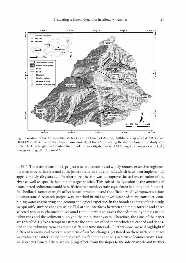
Fig. 1. Location of the Johnsbachtal Valley (with inset map of Austria), hillshade map of a LiDAR derived DEM (2010, © Bureau of the Styrian Government) of the ZMS showing the distribution of the study sites (note: black rectangles with dashed lines mark the investigated areas): (A) Gseng, (B) Langgries outlet, (C) Langgries long, (D) Unnamed V.


on to the main river. (3) Finally we will analyze the time intervals of our laser scan surveys to find out the appropriate survey density needed to quantify sediment dynamics as completely as possible.

2 Study area

2.1 General overview

The Johnsbach Valley is a non-glaciated alpine catchment in Upper Styria, Austria (Fig. 1). It covers an area of approximately 65 km2 in size reaching from 584 m a.s.l. at the outlet to 2369 m a.s.l. (Hochtor). The valley is drained by the Johnsbach River which originates in crystalline bedrock. It runs for 14.1 km with a mean gradient of 3.7 % before it empties into the River Enns. The geological setting in the Johnsbach Valley is characterised by different rocks belonging to two nappes, the Northern Calcareous Alps (NCA) and the Greywacke Zone (GWZ) (e.g. Ampferer 1935, Hiessleitner 1935, 1958, Flügel & Neubauer 1984). A WNW-SES striking tectonic contact zone is separating the NCA in the north and the GWZ in the south. Trias-sic carbonate rocks, mainly limestone (Dachsteinkalk) and dolomite (Wettersteindolomit) are widespread in the NCA in which our area of investigation is situated. In its lower section, the river flows through the “Zwischenmäuerstrecke” (ZMS), a 5 km river reach dominated by cal-careous bedrock. This area is sparsely vegetated by fir forests and pine shrub lands, and shaped by steep furrows and deeply incised channels running into the Johnsbach River from both sides. The majority of the sediment that is relocated and transported in the Johnsbach Valley is stored in the ZMS.

The climate is characterized by annual mean temperatures of around 8 °C in the lower elevations of the valley and below 0 °C in the summit regions. Annual precipitation amounts to approximately 1.500 –1.800 mm (Wakonigg 2012a, b). Storm precipitation occurs almost ex-clusively in the summer months and can reach several tens of mm per hour. Thus, runoff at the Johnsbach River peaks in spring (snow melt) and summer while the tributary trenches show surface runoff and sediment transport only during episodic rainstorms.

The geological situation together with the climatic conditions results in a high morphody-namic activity, primarily in the ZMS (Strasser et al. 2013). The characteristics of carbonate rocks, mainly the brittle Wettersteindolomit which is especially prone to weathering, invoke that large amounts of sharp-edged debris are provided by weathering processes. The steeply sloping terrain is a precondition for the relocation of sediments by rock slides, rock falls or debris avalanches. In the next step of the cascade, mainly incisional processes rework those de-posits on the hillslopes and are responsible for high input rates into the Johnsbach River. That is why the course of the river has been armed with longitudinal barriers and check dams almost 60 years ago. During the aforementioned river-ecological LIFE project controlled by the Gesäuse National Park (Haseke 2011) the river has been renaturated and is now able to transport bed-load continuously. Accordingly, morphological structures in the river have changed to a large extent, resulting in a near-natural situation in the ZMS. Thus, the investigation of connectiv-ity between the tributary channels and the main river is of high practical interest to evaluate the ecological aims of the LIFE project. Due to former gravel mining and to undersized bridge openings, still not all of the side channels are fully coupled to the main river.


Table 1. Catchment characteristics for the three subcatchments as well as the study areas in between.

Sub-catchment

Sub-area Sub-section Area [ha] Slope [°] mean

Altitude [m] Relief energy [m

ha–1]

Gseng

total 113.78 45 619 1,623 1,004 9

study site

total 2.34 29 710 868 158 68top (I) 0.98 30 786 851 65 66middle (II) 0.86 30 749 868 119 138bottom (III) 0.50 26 710 758 48 96

Langgries

total 330.15 45 650 2,251 1,601 5study site outlet total 0.21 16 650 666 16 76

total 3.01 16 663 769 106 35

study site long

top (I) 0.88 22 720 769 49 56middle-top (II) 0.79 16 695 728 33 42middle-bottom (III) 0.85 13 677 701 24 28bottom (IV 0.49 12 663 680 17 35

Unnamed V

total 15.75 60 682 1,358 676 43

study sitetotal 0.16 21 682 708 26 163top (I) 0.12 22 685 708 23 192bottom (II) 0.04 17 682 688 6 150

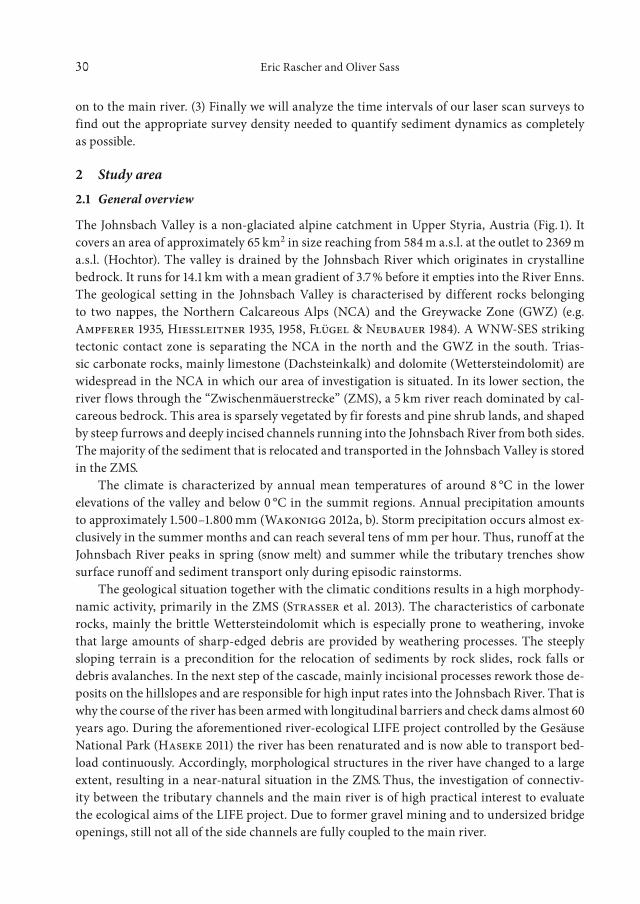
Fig. 2. Photographs of the study sites in the Johnsbach Valley: (A) Gseng in an eastward direction (26th July 2013) with inset (side-inverted) of the middle part (17th July 2014) during a severe thunder storm (photo taken by Oliver Gulas); (B) Langgries Outlet recorded from the road bridge on the west: top (17th September 2013), bottom (26th August 2015); (C) looking west into Langgries long (28th July 2013), note: the road bridge in the front and the Admonter Reichenstein in the back, the white rectangle locates the site of Langgries outlet; (D) the outlet of Unnamed V from the west: left (18th March 2014), right (26th August 2015). Note: red lines showing the areas of investigation, numbers are indicating the subsections as defined in Tab. 1, blue arrows indicate the flow direction of the Johnsbach River.


2.2 Zones of interest

Volume changes of four study sites (Figs. 1, 2 and Table 1) were investigated between September 2013 and October 2015. The sites are located in between or at the outlet of three different side channels. The site Unnamed V is in the southern part of the ZMS which is dominated by steep dolomite rock walls. The focus is on the mouth of the side channel to find out how this tributary is coupled to the main channel. Further north, the dolomite is covered by breccia which protects the underlying rocks from erosion and results in a smoother landscape with lower gradients (Lieb & Premm 2008). In this area, the study sites Langgries and Gseng are located. The two channels are the largest ones in the ZMS and contain the most debris. Different companies were mining this debris starting in 1984 in the Gseng trench and in 1991 at Langgries, respectively. In 2002 the Gesäuse National Park was established but due to running lease agreements the gravel mining was finally stopped in 2005. Up to now it cannot be assessed how much sediment was excavated during that mining period. Nevertheless, the resulting landscape modifications in both side channels are surface lowering and a change in slope of the former continuous sedi-ment body. Thus, sediment routing in those two channels is still disturbed to some extent and has been slowly returning to near-natural conditions during the last years. At Gseng, the sur-veyed area was set up in the upper part of the trench (some 100 m above the confluence with the

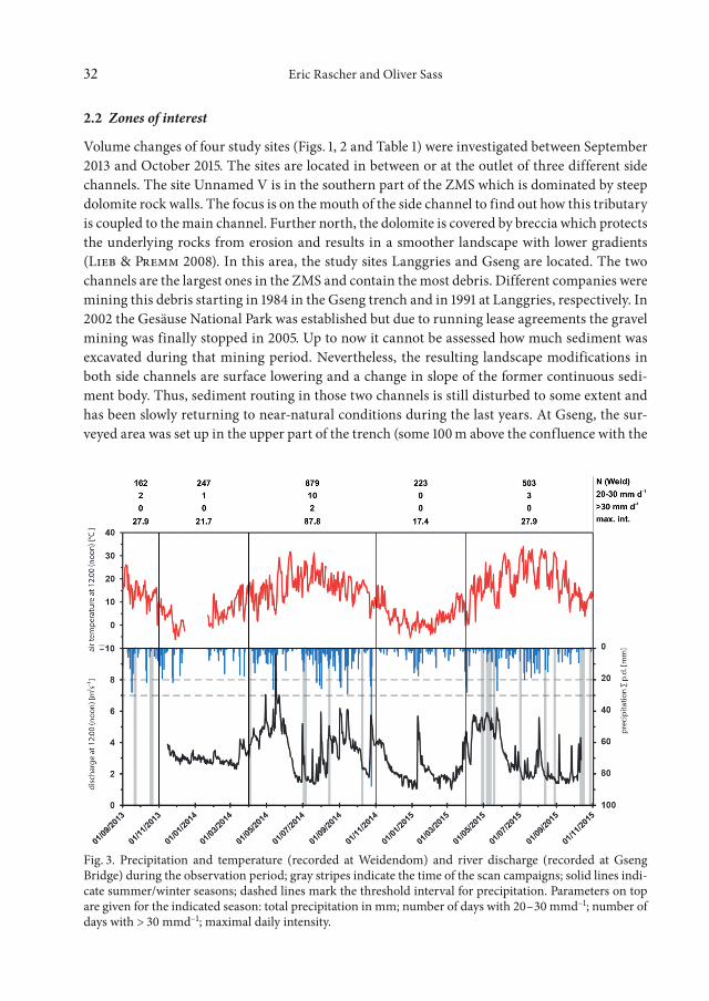
Fig. 3. Precipitation and temperature (recorded at Weidendom) and river discharge (recorded at Gseng Bridge) during the observation period; gray stripes indicate the time of the scan campaigns; solid lines indi-cate summer/winter seasons; dashed lines mark the threshold interval for precipitation. Parameters on top are given for the indicated season: total precipitation in mm; number of days with 20 – 30 mmd–1; number of days with > 30 mmd–1; maximal daily intensity.


Johnsbach River) where the hillslopes are contributing sediment into the side channel forming a sediment body, which is moving slowly down to where the former mining factory (Fig. 1) was set up. The factory has been dismantled in 2008 but the area around is still too flat to allow sedi-ment movement across the site, obviously decoupling the active part of the Gseng trench from the main river system. Langgries is a very long sediment body moving slowly downhill. In this sub-catchment, two study sites were surveyed: the immediate confluence with the Johnsbach River below the road bridge and several 100 m long, inclined gravel field upstream to the bridge. This allowed studying coupling effects at the outlet of the system, sediment dynamics inside the trenches and sediment supply from the lateral slopes.

The weather conditions and the river discharge during the observation period are depicted in Fig. 3. The location of the weather and the gauging station are shown in Fig. 1. Air tempera-tures ranged from –11 °C to 34 °C in the observation period with a mean of 8.4 °C and rainfall was almost evenly distributed during summer and winter seasons with an annual amount of ~930 mm. The river discharge of the Johnsbach River had a base flow of ~1, a mean of ~3, and peaks of ~6 –10 m3s–1. Missing discharge values in September and October 2013 as well as data gaps in the temperature record in December 2013 are due to failures of the recording instru-ments.

3 Data acquisition and processing

3.1 Terrestrial laser scanning in the field

Terrestrial laser scan surveys were carried out using a Riegl LMS-Z620 and the Riegl Software RiScanPro (v.2.1.1) for data acquisition. The laser scanner has a minimum distance of 2 m and a maximum range of up to 2,000 m by measurement rates up to 11,000 pts s–1. The used wave length is 1,500 nm with a beam divergence of 0.15 mrad (Riegl 2010).

At each scan position the scanner was mounted on a tripod as high as possible to reduce shadowing effects. Prior to the measurement, the system was levelled coarsely to approx. 1° and finally stabilized by the built-in inclination sensors. Reflector targets (10 cm Ø cylinder) were drilled into rocks or mounted on trees if no rock walls were accessible to mutually register sin-gle scans from one scan campaign and among different scan periods. Usually 4 –7 targets were spread out covering the field sites in all directions and angles. To reduce shadowing effects the area of interest (AOI) was scanned overlapping from multiple scan positions at different resolu-tions depending on the size of the AOI and the distances in between (Table 2). Multi temporal scans were performed 4 – 5 times during the observation period (Fig. 3) usually in the beginning (after snowmelt) and end (before snowfall) of the summer season. Additionally, pictures were taken using a mounted camera (Nikon D300) during the first field campaign to overlay each point in the point cloud with its color code (RGB value).

3.2 From scan registration to DEM creation

Data post processing was achieved using the Riegl Software RiScanPro (v.2.1.1) as well as Arc-GIS (v.10.1). The scan positions were registered in RiScanPro using the scanned reflector targets from each scan campaign. Afterwards all scans from one site and scan period were aligned


resulting in one major scan. The scans still remain in their scanner’s own coordinate system for dGPS measurements were not taken because of poor signal strength in the field and also because additional errors might be included due to transformation processes. Finally the AOI was separated from the unimportant area around.

To eliminate vegetation and “flying points” the terrain filter in RiScanPro was applied to separate off-terrain points. The filter works in a hierarchic manner with several levels of detail using a coarse-to-fine approach and is based on a grid representation of the data at each level. Representative cell points (RCP) are selected and used to estimate a local surface and therefore a robust plane through the central cells RCPs and its neighbors. A tolerance range for each cell above/below this plane specifies points as “off-terrain”. All remaining points are assigned to new cells in the next finer level where the process starts again (Riegl 2010). For each scan site the results of the filtering were optimized by adjusting the base grid size, the number of levels and the tolerance value when comparing to the color coding of the scans and pictures taken in the field.

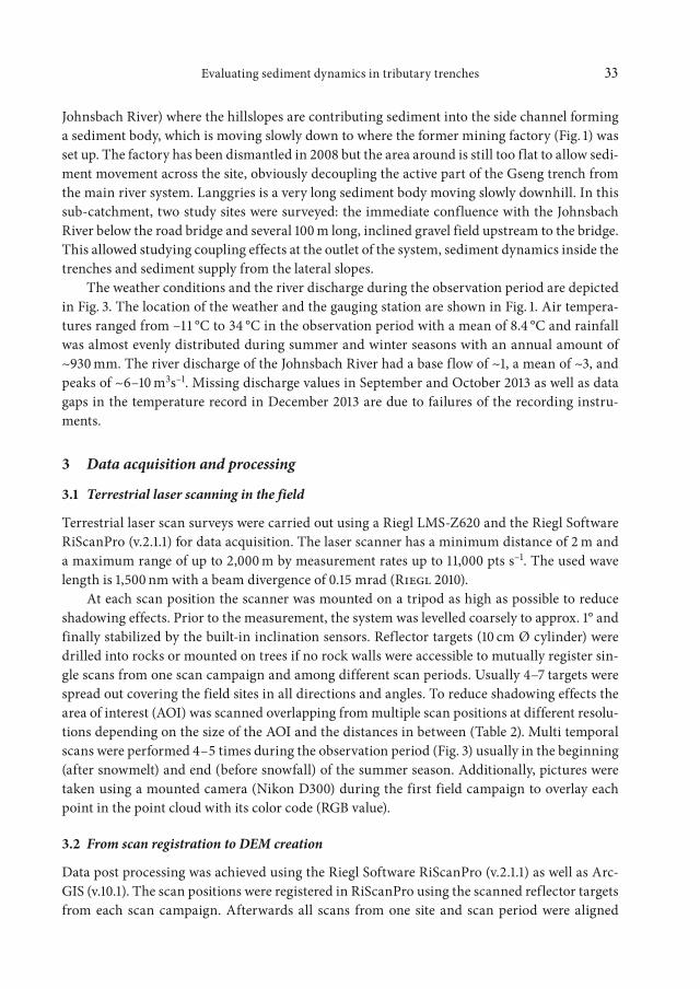
Table 2: Information on the scan properties as well as results for alignment procedures for all study sites and survey periods.

Survey site Survey date Positions Distance Angular Resolutiona

Pointsb SDRc Points AOId Point density

Cell size SDEe

(mean) (mean) (total) (mean) (total) (mean)

[m] [m] [in Mio] [in Mio] [in Mio] % [points m– 2] [cm] [cm]

Gseng

22.09.2013 3 270 0.15 31.3 1.0 17.2 55 733 20.0 0.803.04.2014 3 270 0.15 29.4 0.7 16.4 56 698 20.0 0.709.10.2014 3 280 0.15 30.7 0.9 13.7 45 582 20.0 0.829.04.2014 4 225 0.16 23.1 0.6 15.5 67 659 20.0 0.412.10.2015 4 240 0.16 42.0 0.7 18.9 45 807 20.0 0.6

Langries outlet

21.09.2013 3 40 0.03 16.1 0.6 8.9 55 4,339 5.0 0.503.07.2014 3 70 0.05 18.3 0.5 10.9 60 5,321 5.0 0.507.05.2015 3 70 0.05 21.7 0.8 12.5 58 6,074 5.0 0.512.10.2015 3 70 0.05 17.4 0.6 9.6 55 4,667 5.0 0.5

Langries long

21.09.2013 2 350 0.20 17.4 0.7 7.8 45 261 20.0 1.204.07.2014 2 375 0.20 17.8 1.1 8.0 45 268 20.0 1.430.04.2015 4 300 0.19 25.9 0.8 15.3 59 511 20.0 0.813.10.2015 4 300 0.17 39.3 0.9 18.0 46 599 20.0 0.6

Unnamed V

20.10.2013 4 70 0.05 21.2 0.8 7.4 35 4,558 5.0 0.814.08.2014 4 70 0.05 19.5 0.6 6.3 32 3,848 5.0 1.111.05.2015 4 70 0.05 21.3 0.6 6.6 31 4,064 5.0 0.728.08.2015 4 70 0.05 31.3 0.6 7.3 23 4,512 5.0 0.827.10.2015 4 70 0.05 24.8 0.6 6.3 25 3,858 5.0 0.8

a: Mean angular resolution refers to the mean distance.b: Total amount of points recorded from all scan positions.c: Standard deviation after registration of all scan positions.d: Total amount of points inside the AOI after eliminating the vegetation, percentages are in terms of

total amount of points recorded.e: Standard deviation of error.


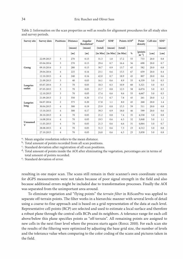
In ArcGIS all point clouds were interpolated to triangulated irregular networks from which DEMs were produced with cell sizes of 5 cm and 20 cm (Table 2) respectively. To estimate the error of TLS data and thus managing DEM uncertainties, a minimum level of detection (LoD) threshold to separate actual surface changes from the inherent noise was applied (Wheaton et al. 2010). We therefore follow the existing approaches for propagating uncertainties in Digital Elevation Models of Difference (DoDs) (Taylor 1997, Brasington et al. 2003, Fuller et al. 2003, Lane et al. 2003) which were summarized by Wheaton et al. (2010). The approximation of the standard deviation of error (SDE) is a reasonable estimate of the uncertainty of the verti-cal component (δz) which leads to:

(1)

where Ucrit is the critical threshold error (LoD) based on a critical Student’s t-value at a chosen confidence interval. Throughout this paper, the 95 % confidence interval is used as a threshold which leads to a t-value of 1.96. To estimate δz the original point clouds were cut in half (with random point pick). Afterwards the same workflow was applied, as to the original point clouds, resulting in two DEMs (raster cell size according to original DEM) for one survey. Using those two DEMs standard deviations were estimated (Table 2) for each survey. By applying equation (1) a LoD value was calculated for each raster cell for the survey period A–B to gain a spatially distributed error across the DEM (Milan et al. 2011). Elevation changes in between a range of +/– LoD were discarded whereas changes outside of these limits were accepted.

U�� (1)

Table 3. Summary of uncertainty range values of each raster cell.

Study site Period Raster Count (of AOI)

LoD [m]min max mean

Gseng

Sep. 2013 – April 2014 586,669 0 2.88 0.02April 2014 – Oct. 2014 586.669 0 2.75 0.02Oct. 2014 – April 2015 586.669 0 5.38 0.02April 2015 – Oct. 2015 586.670 0 5.38 0.02Sep. 2013 – Oct. 2015 586.669 0 2.43 0.02

Langgries Outlet

Sep. 2013 – July 2014 821,043 0 1.20 0.02July 2014 – May 2015 821,046 0 1.96 0.02May 2015 – Oct. 2015 821,046 0 1.97 0.02Sep. 2013 – Oct. 2015 821,043 0 1.22 0.02

Langgries long

Sep. 2013 – July 2014 751.710 0 6.11 0.04July 2014 – April 2015 751.710 0 6.11 0.04April 2015 – Oct. 2015 751.709 0 7.27 0.02Sep. 2013 – Oct. 2015 751.709 0 7.27 0.03

Unnamed V

Oct. 2013 – Aug. 2014 650.625 0 1.16 0.03Aug. 2014 – May 2015 650.623 0 1.16 0.03May 2015 – Aug. 2015 650.623 0 1.02 0.03Aug. 2015 – Oct. 2015 650.625 0 0.99 0.03Oct. 2013 – Oct. 2015 650.626 0 1.06 0.03


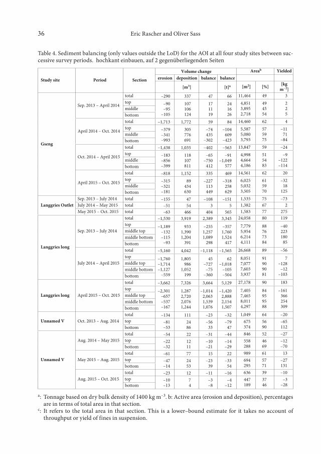
Table 4. Sediment balancing (only values outside the LoD) for the AOI at all four study sites between suc-cessive survey periods. hochkant einbauen, auf 2 gegenüberliegenden Seiten

Study site Period Section

Volume change Areab Yieldederosion deposition balance balance

[m3] [t]a [m2] [%] [kg m– 2]

Gseng

Sep. 2013 – April 2014

total –290 337 47 66 11,464 49 3top –90

–95–105

107106124

171119

241626

4,8513,8952,718

494554

225

middlebottom

April 2014 – Oct. 2014

total –1,713 1,772 59 84 14,460 62 4top –379

–341–993

305776691

–74435

–302

–104609

–423

5,5875,0803,793

575975

–1171

–84middlebottom

Oct. 2014 – April 2015

total –1,438 1,035 –402 –563 13,847 59 –24top –183

–856–399

118107811

–65–750

412

–91–1,049

577

4,9984,6644,186

515483

–9–122–114

middlebottom

April 2015 – Oct. 2015

total –818 1,152 335 469 14,561 62 20top –315

–321–181

89434630

–227113449

–318258629

6,0255,0323,505

615970

–3218

125middlebottom

Langgries OutletSep. 2013 – July 2014 total –155 47 –108 –151 1,535 75 –73July 2014 – May 2015 total –51 54 3 5 1,382 67 2May 2015 – Oct. 2015 total –63 466 404 565 1,583 77 275

Langgries long

Sep. 2013 – July 2014

total –1,530 3,919 2,389 3,345 24,058 80 119top –1,189

–132–115

–93

9331,3901,204

391

–2551,2571,089

298

–3571,7601,524

417

7,7795,9546,2144,111

88767384

–40223180

85

middle topmiddle bottombottom

July 2014 – April 2015

total –5,160 4,042 –1,118 –1,565 26,668 89 –56top –1,760

–1,714–1,127

–559

1,805986

1,052199

45–727

–75–360

62–1,018

–105–504

8,0517,0777,6033,937

91909081

7–128

–12–103


Langgries long April 2015 – Oct. 2015

total –3,662 7,326 3,664 5,129 27,178 90 183top –2,301

–657–537–167

1,2872,7202,0761,244

–1,0142,0631,5391,076

–1,4202,8882,1541,507

7,4057,4658,0114,297

84959588

–161366254309


Unnamed V Oct. 2013 – Aug. 2014total –134 111 –23 –32 1,049 64 –20top –81

–532486

–5633

–7947

675374

5690

–65112bottom

Unnamed V

Aug. 2014 – May 2015total –54 22 –31 –44 846 52 –27top –22

–321211

–10–21

–14–29

558288

4669

–12–70bottom

May 2015 – Aug. 2015total –61 77 15 22 989 61 13top –47

–142453

–2339

–3354

694295

5771

–27131bottom

Aug. 2015 – Oct. 2015total –23 12 –11 –16 636 39 –10top –10

–1374

–3–8

–4–12

447189

3746

–3–28bottom

a: Tonnage based on dry bulk density of 1400 kg m– 3. b: Active area (erosion and deposition), percentages are in terms of total area in that section.

c: It refers to the total area in that section. This is a lower–bound estimate for it takes no account of throughput or yield of fines in suspension.


4 Results

DEM analysis of all four investigated areas indicates variations in sediment mobility during all time steps. These seasonal surveys show that different patterns of erosion and deposition can be detected when compared to the overall result of a two year investigation period. The uncertainty range (LoD) varies for each raster cell, survey interval and study site (Table 3). An overview of all data is provided in Table 4. The classification into subdivisions of the respective study sites is not following any particular rule and has been done to quantify how much sedi-ment is being moved within each system. The term “active area” is assigned to the parts of the investigated region in which surface change between two surveys is above the range of +/– LoD.

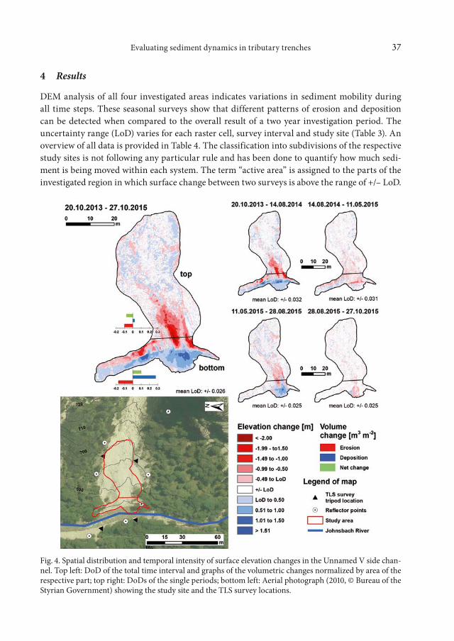
Fig. 4. Spatial distribution and temporal intensity of surface elevation changes in the Unnamed V side chan-nel. Top left: DoD of the total time interval and graphs of the volumetric changes normalized by area of the respective part; top right: DoDs of the single periods; bottom left: Aerial photograph (2010, © Bureau of the Styrian Government) showing the study site and the TLS survey locations.


4.1 Unnamed V

Patterns of erosion and deposition are mostly limited to the bottom part (next to the river) as well as the lower parts of the top section (Fig. 4). This is also reflected in the size of the active area throughout all time steps which is around 50 % for the top and 70 % for the bottom part. During the first period (from October 2013 to August 2014) erosion took place mainly in the upper steep parts of the bottom section which form the front of the side channel at the conflu-ence with the main river. Additionally the side channel was deeply incised (up to 1.5 m) in the center between upper and lower part. However the majority of the mobilized sediment was still accumulated at the outlet of the side channel and only a small amount (23 m3) made its way out of the subsystem. In the following period (till May 2015) the upper section did not show any significant changes whereas bank erosion represented most of the sediment loss. Almost two-thirds of the sediment in motion was transported into the river. In the summer of 2015a slope failure caused the formation of a fan (with a volume of around 50 m3) developing into the John-sbach River almost over the entire width (Fig. 2D). Elevation changes were ranging from –1.5 m to 1.0 m at prominent spots. From that time the fan was successively eroded by the river (August – October 2015) whereas a small part behind the fan (in flow direction) was filled up with that material. In the remaining parts of the investigated area no significant changes were observed.

4.2 Langgries outlet

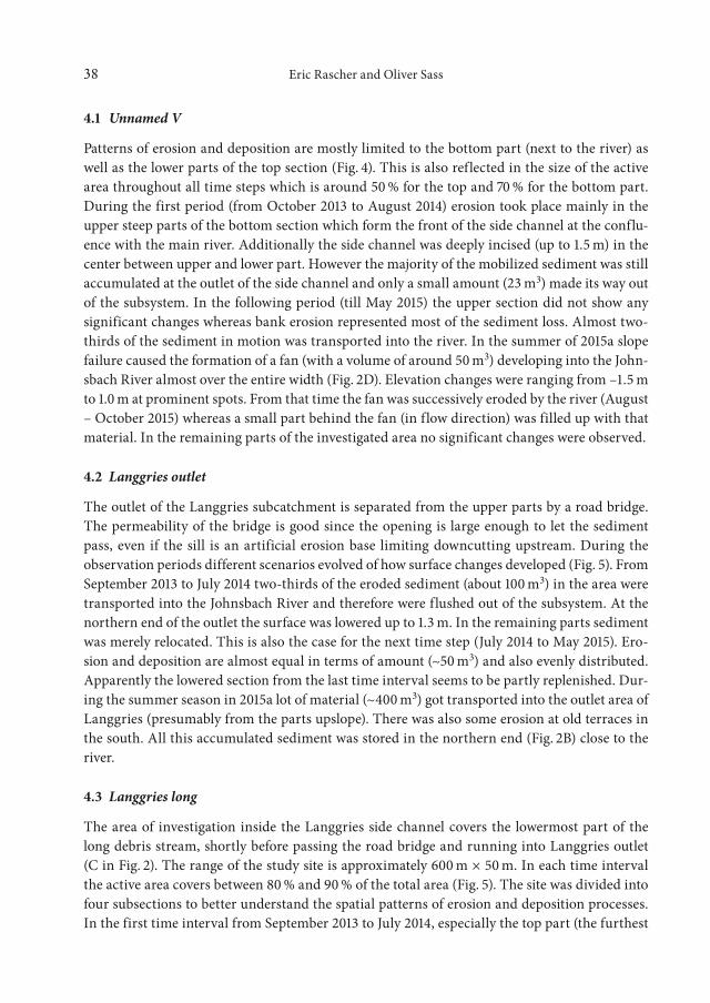
The outlet of the Langgries subcatchment is separated from the upper parts by a road bridge. The permeability of the bridge is good since the opening is large enough to let the sediment pass, even if the sill is an artificial erosion base limiting downcutting upstream. During the observation periods different scenarios evolved of how surface changes developed (Fig. 5). From September 2013 to July 2014 two-thirds of the eroded sediment (about 100 m3) in the area were transported into the Johnsbach River and therefore were flushed out of the subsystem. At the northern end of the outlet the surface was lowered up to 1.3 m. In the remaining parts sediment was merely relocated. This is also the case for the next time step (July 2014 to May 2015). Ero-sion and deposition are almost equal in terms of amount (~50 m3) and also evenly distributed. Apparently the lowered section from the last time interval seems to be partly replenished. Dur-ing the summer season in 2015a lot of material (~400 m3) got transported into the outlet area of Langgries (presumably from the parts upslope). There was also some erosion at old terraces in the south. All this accumulated sediment was stored in the northern end (Fig. 2B) close to the river.

4.3 Langgries long

The area of investigation inside the Langgries side channel covers the lowermost part of the long debris stream, shortly before passing the road bridge and running into Langgries outlet (C in Fig. 2). The range of the study site is approximately 600 m × 50 m. In each time interval the active area covers between 80 % and 90 % of the total area (Fig. 5). The site was divided into four subsections to better understand the spatial patterns of erosion and deposition processes. In the first time interval from September 2013 to July 2014, especially the top part (the furthest


Fig. 5. Spatial distribution and temporal intensity of surface elevation changes in the Langgries side chan-nel. Top: DoD for the total time interval as well as for the three periods for the study sites Langgries long (left) and Langgries outlet (right), included are graphs of the volumetric changes normalized by area of the respective part, bottom: Aerial photograph (2010, © Bureau of the Styrian Government) showing the study sites and the TLS survey locations.


west) is characterized by major erosion. This can be allocated to the lateral slopes in the north and due to incision of ~1.5 m deep channels in the central parts. The two sections in the middle show a similar and even distribution of changes with erosion being nearly one-tenth of the total relocated material. In the bottom part, close to the bridge, erosion takes place streamlined in the center. Deposition (around 400 m3) is rather uniform across the rest of the section and is four times higher than erosion (~100 m3). During the following period (July 2014 to April 2015) there is an overbalance of erosion almost over the entire area of investigation. Especially in the parts ‘middle-top’ and ‘bottom’ the relation between cut and fill is about 1:2. The other two parts

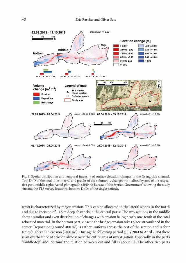
Fig. 6. Spatial distribution and temporal intensity of surface elevation changes in the Gseng side channel. Top: DoD of the total time interval and graphs of the volumetric changes normalized by area of the respec-tive part, middle right: Aerial photograph (2010, © Bureau of the Styrian Government) showing the study site and the TLS survey locations, bottom: DoDs of the single periods.


show a nearly equal distribution of erosion and deposition. In the top section, incision ranges down to 2.5 m whilst deposition reaches up to 1.5 m. The last interval including the summer and autumn of 2015 is characterized by a positive volume balance in the middle and bottom parts whereas the top shows large areas of sediment loss. This incision is channelized to a couple of pathways, between which new material is stored. In the three sections downstream deposition continuously outranges erosion by a factor of 4 (both middle sections) and 8 (bottom section) respectively. The source areas of sediment are limited mostly to the lateral slopes while deposi-tion occurs area-wide in the central zones.

4.4 Gseng

The area of investigation in the Gseng subcatchment consists of a debris stream with its adjacent hillslopes (A in Fig. 2). However, changes in surface elevation are mainly restricted to the central trench (Fig. 6). From September 2013 to April 2014 all three sections show minor redistribution of sediment with amounts of erosion and deposition almost being balanced. In each section the active areas cover 50 % of the total area. During the summer season of 2014 (April to October) each part was behaving differently. In the ‘top’ erosion and deposition were nearly balanced. The hillslope was barely affected and the changes only occurred in the central trench. The other two parts show an opposite behavior as the ‘middle’ is characterized by a net balance of about +435 m3 and the ‘bottom’ loosing around –302 m3. Primary areas of surface change are in the central thalweg during this period. The interval from October 2014 to April 2015 shows major incision of up to 2 m in the middle part resulting in a net balance of approx. –750 m3. Con-versely, the bottom section has gained +412 m3 by accumulating almost 2 m in some places. In the top region cut and fill are almost equal at values of around 180 m3 and 120 m3, respectively. During the summer season of 2015 (April to October) the net change shifts from a negative bal-ance (–227 m³) in the upper part over a nearly balanced part in the middle (113 m³) to a positive balance (449 m³) in the lower section. Through all parts surface changes occur again mostly in the central flow path. Areas of higher erosion (up to 1.5 m) are isolated and restricted to the mid-dle part whereas areas of deposition are mainly in the transition zone between the middle and the bottom part and in the lower bottom part with surface changes of up to 2 m.

4.5 Summary of the rates of relocated sediment

Combining all four study sites total sums of ~7400 m3 yr–1 were eroded in the surveyed areas and ~9900 m3 yr–1 were deposited when the 2-yr observation period is used as a basis. Ero-sion is divided into ~2070 m3 yr–1 at Gseng, ~130 m3 yr–1 at Langgries Outlet, ~5020 m3 yr–1 at Langgries long and ~140 m3 yr–1 at Unnamed V; deposition is split into ~2090 m3 yr–1 at Gseng, ~280 m3 yr–1 at Langgries Outlet, ~7420 m3 yr–1 at Langgries long and ~110 m3 yr–1 at Unnamed V. This results in an overall net rate of +0.044 m3m– 2 yr–1 (–0.13 m3m– 2 yr–1 of area-wide erosion and +0.17 m3m– 2 yr–1 of area-wide sedimentation) in the investigated sections (+0.001 m3m– 2 yr–1 at Gseng,+0.071 m3m– 2 yr–1 at Langgries outlet,+0.080 m3m– 2 yr–1 at Langgries long and –0.015 m3m– 2 yr–1 at Unnamed V). The majority of the relocated sediment was merely redistrib-uted inside the trenches and thus was not delivered to the Johnsbach River. Only a minimum amount of ~650 m3 yr–1 was delivered to the river (~620 m3 yr–1 at Langgries, ~30 m3 yr–1 at


Unnamed V and none at Gseng) not taking into account if these sediments have actually been taken up by the river or not. The amounts of sediment that have entered the areas of observation from above and have passed through the system without leaving a trace in the laser scans are

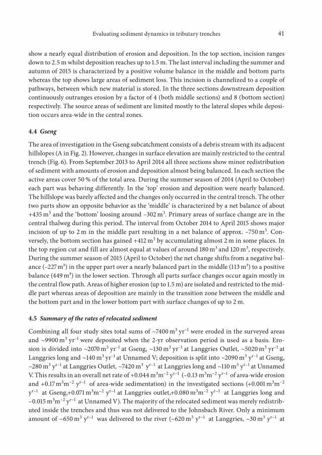
Fig. 7. Temporal development of the sediment yield distributed by subsections for each study site; I–IV refer to the subsections as defined in Fig. 2 and Table 1; solid lines separate the total from the single intervals; dashed lines separate the stepwise approach. Precipitation parameters are given for the respective interval: total precipitation in mm (Weidendom); number of days with 20 – 30 mmd–1; number of days with > 30 mmd–1; maximal daily intensity.


still unknown. Thus, the mentioned quantities are the minimum amount of debris which has been delivered to the river. A detailed description of the sediment yield for each survey period and study site is given in Fig. 7.

4.6 Comparison of volume changes and active areas considering different time intervals

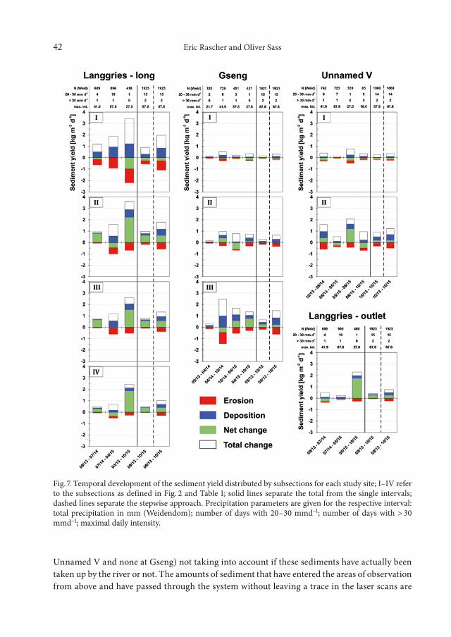
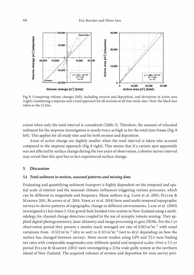
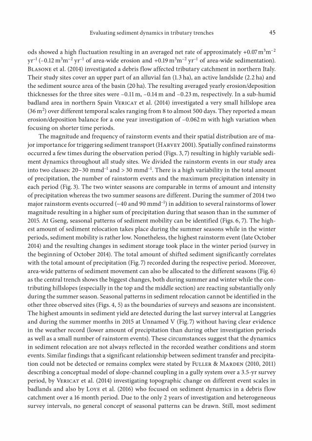
The spatial distribution of surface elevation changes are depicted in Figs. 4 to 6 for the differ-ent single survey intervals (“stepwise”) and the total investigation period (“total”) considering only the first and last survey for each study site. The time frame of the total investigation covers approximately two years at each study site (September/October 2013 to October 2015). In the stepwise investigation, shifts in erosional and depositional patterns are cancelled out to some

Table 5. Sediment balancing (only values outside the LoD) for the AOI at all four study sites for the overall investigation period (comparing the first to the last survey). Values in italics also consider all surveys made in between.

Study site Period Section

Volume change Area Yieldederosion deposition balance balance

[m3] [t]a [m2] [%] [kg m– 2]

Gseng

Sep. 2013 – Oct. 2015

total –1,937 2,066 129 180 16,695 71 8top –600 246 –355 –496 6,424 65 –50middle –788 591 –198 –277 6,162 72 –32bottom –549 1,229 681 953 4,109 82 189

Sep. 2013 – Oct. 2015

total –4,258 4,297 39 55 21,763 93 2top –967 618 –349 –489 9,034 92 –50middle –1,614 1,423 –190 –266 7,836 91 –32bottom –1,677 2,255 578 809 4,893 97 161

Langgries OutletSep. 2013 – Oct. 2015 total –72 373 302 423 1,709 83 206Sep. 2013 – Oct. 2015 total –268 567 300 419 1,886 92 204

Langgries long

Sep. 2013 – Oct. 2015

total –4,109 9,125 5,016 7,022 28,147 94 234top –2,695 1,469 –1,226 –1,716 8,186 93 –194middle top –726 3,393 2,631 3,684 7,524 95 467middle bottom –506 3,097 2,592 3,628 7,941 94 428bottom –147 1,166 1,019 1,426 4,494 92 292

Sep. 2013 – Oct. 2015

total –10,352 15,287 4,935 6,909 29,484 98 230top –5,250 4,025 1,225 1,715 8,566 97 –194middle top –2,503 5,096 2,593 3,630 7.781 99 460middle bottom –1,779 4,332 2,553 3,574 8,341 98 422bottom –820 1,834 1,014 1,420 4,796 98 291

Unnamed V

Oct. 2013 – Oct. 2015total –195 144 –51 –71 1,206 74 –44top –123 30 –94 –131 812 67 –108bottom –72 115 42 59 394 95 143

Oct. 2013 – Oct. 2015total –272 222 –50 –70 1,476 91 –43top –160 67 –93 –130 1,066 88 –107bottom –111 154 43 60 411 99 144

a: Tonnage based on dry bulk density of 1,400 kg m– 3.


extent when only the total interval is considered (Table 5). Therefore, the amount of relocated sediment for the stepwise investigation is nearly twice as high as for the total time frame (Fig. 8 left). This applies for all study sites and for both erosion and deposition.

Areas of active change are slightly smaller when the total interval is taken into account compared to the stepwise approach (Fig. 8 right). This means that if a certain spot apparently was not affected by surface change during the two years of observation, a shorter survey interval may reveal that this spot has in fact experienced surface change.

5 Discussion

5.1 Total sediment in motion, seasonal patterns and missing data

Evaluating and quantifying sediment transport is highly dependent on the temporal and spa-tial scale of interest and the seasonal climatic influences triggering various processes, which can be different in magnitude and frequency. Many authors (e.g. Lane et al. 2003, Fuller & Marden 2011, Blasone et al. 2014, Vericat et al. 2014) have used multi-temporal topographic surveys to derive patterns of topographic change in different environments. Lane et al. (2003) investigated a 1 km times 3.3 km gravel-bed, braided river system in New Zealand using a meth-odology for channel change detection coupled to the use of synoptic remote sensing. They ap-plied digital photogrammetry, laser altimetry and image processing to gain DEMs. For the 1-yr observation period they present a similar reach averaged net rate of 0.013 m3m– 2 with zonal variations from –0.523 m3m– 2 (dry to wet) to 0.513 m3m– 2 (wet to dry) depending on how the surface has changed between surveys. More recent studies using GPS and TLS were finding net rates with comparable magnitudes over different spatial and temporal scales. Over a 3.5-yr period Fuller & Marden (2011) were investigating a 21 ha wide gully system at the northern island of New Zealand. The acquired volumes of erosion and deposition for nine survey peri-

Fig. 8. Comparing volume changes (left), including erosion and deposition, and deviations in active area (right) considering a stepwise and a total approach for all sections at all four study sites. Note: the black line refers to the 1:1 line.


ods showed a high fluctuation resulting in an averaged net rate of approximately +0.07 m3m– 2

yr–1 (–0.12 m3m– 2 yr–1 of area-wide erosion and +0.19 m3m– 2 yr–1 of area-wide sedimentation). Blasone et al. (2014) investigated a debris flow affected tributary catchment in northern Italy. Their study sites cover an upper part of an alluvial fan (1.3 ha), an active landslide (2.2 ha) and the sediment source area of the basin (20 ha). The resulting averaged yearly erosion/deposition thicknesses for the three sites were –0.11 m, –0.14 m and –0.23 m, respectively. In a sub-humid badland area in northern Spain Vericat et al. (2014) investigated a very small hillslope area (36 m2) over different temporal scales ranging from 8 to almost 500 days. They reported a mean erosion/deposition balance for a one year investigation of –0.062 m with high variation when focusing on shorter time periods.

The magnitude and frequency of rainstorm events and their spatial distribution are of ma-jor importance for triggering sediment transport (Harvey 2001). Spatially confined rainstorms occurred a few times during the observation period (Figs. 3, 7) resulting in highly variable sedi-ment dynamics throughout all study sites. We divided the rainstorm events in our study area into two classes: 20 – 30 mmd–1 and > 30 mmd–1. There is a high variability in the total amount of precipitation, the number of rainstorm events and the maximum precipitation intensity in each period (Fig. 3). The two winter seasons are comparable in terms of amount and intensity of precipitation whereas the two summer seasons are different. During the summer of 2014 two major rainstorm events occurred (~40 and 90 mmd–1) in addition to several rainstorms of lower magnitude resulting in a higher sum of precipitation during that season than in the summer of 2015. At Gseng, seasonal patterns of sediment mobility can be identified (Figs. 6, 7). The high-est amount of sediment relocation takes place during the summer seasons while in the winter periods, sediment mobility is rather low. Nonetheless, the highest rainstorm event (late October 2014) and the resulting changes in sediment storage took place in the winter period (survey in the beginning of October 2014). The total amount of shifted sediment significantly correlates with the total amount of precipitation (Fig. 7) recorded during the respective period. Moreover, area-wide patterns of sediment movement can also be allocated to the different seasons (Fig. 6) as the central trench shows the biggest changes, both during summer and winter while the con-tributing hillslopes (especially in the top and the middle section) are reacting substantially only during the summer season. Seasonal patterns in sediment relocation cannot be identified in the other three observed sites (Figs. 4, 5) as the boundaries of surveys and seasons are inconsistent. The highest amounts in sediment yield are detected during the last survey interval at Langgries and during the summer months in 2015 at Unnamed V (Fig. 7) without having clear evidence in the weather record (lower amount of precipitation than during other investigation periods as well as a small number of rainstorm events). These circumstances suggest that the dynamics in sediment relocation are not always reflected in the recorded weather conditions and storm events. Similar findings that a significant relationship between sediment transfer and precipita-tion could not be detected or remains complex were stated by Fuller & Marden (2010, 2011) describing a conceptual model of slope-channel coupling in a gully system over a 3.5-yr survey period, by Vericat et al. (2014) investigating topographic change on different event scales in badlands and also by Loye et al. (2016) who focused on sediment dynamics in a debris flow catchment over a 16 month period. Due to the only 2 years of investigation and heterogeneous survey intervals, no general concept of seasonal patterns can be drawn. Still, most sediment


throughout all side channels is being moved during the summer seasons which can be related to triggering rainstorm events. Remarkably, the frequency and intensity of storms in the sum-mer of 2014 is significantly higher than in 2015 (Fig. 3, 7), but besides Gseng all investigated sites show a contrary behavior in having more sediment relocated in the summer of 2015 than in 2014. This could be due to the facts that the survey interval is inconsistent between the study sites assigning relocated sediment to different seasons as well as the possibility of single rain-storm events acting only locally and therefore being recorded at the nearby Weidendom station without triggering any geomorphic activity in the study areas or vice versa.

The established relocation rates are a minimum amount as the sums of erosion and deposi-tion over the entire time interval are lower than the cumulated sums of the shorter intervals (Fig. 8). Thus, if the number of surveys would have been higher, the volume of transported sediments would probably increase further. Lane et al. (1994, Fig. 9) stated that a spatial point density of > approx. 3–4 points/m2 is necessary to avoid missing information and that higher densities do not further improve the results. We assume that a similar approach is valid for the temporal density of surveys, since the time dimension is of major importance in studying mass movements (Flageollet 1996) and coupling behavior (Harvey 2002). This means that above a critical amount of surveys a higher sampling frequency would not necessarily improve the results. We could show that an approximately 4-fold higher frequency of surveys (‘step-wise’ approach) results in roughly two times higher volumes of erosion and deposition (both affected almost to the same degree) with effects on the net change being less significant (Fig. 7). This inter-event effect was also determined by Vericat et al. (2014) showing that a reduction of survey frequency results in topographic changes in opposite directions being cancelled out. Comparing surface changes of each survey interval with the total interval (Figs. 4 – 6) reveals different patterns. During longer monitoring periods multiple topographic changes occurring at the event-scale are followed by further topographic changes in an opposite direction. Thus, an event-scale based monitoring should be aspired to avoid “missing” sediment. This “ideal” survey density to capture the (reasonably complete) amount of mobilized sediments (not taking into account if there is sediment transported without leaving a trace in the landscape) depends on the interval between significant, geomorphologically effective rainstorm events. As no de-fined precipitation or runoff threshold for an “effective” rainstorm can be derived from the precipitation data (Fig. 3) and no continuous observation (e.g. webcam) is available this task remains for further investigations.

5.2 Current sediment dynamics of the trenches

Over the entire 2-yr period, debris at Langgries is eroded in the top position of the gravel stream and deposited in the middle and lower reaches (Fig. 5). We assign this effect to an ongoing re-action on the former gravel mining which has lowered the entire trench (as far as it could be reached by caterpillars) and thus, over-steepened the upper parts. If this process continues, sedi-ment output into the river will increase in the future as the reach upstream of the road bridge currently increases in elevation. The deposited amounts in the lower three quarters over-balance the erosion in the uppermost quarter. This can also be due to the bridge opening, which is the lower end of the study site Langgries-long, narrowing the channel and therefore impeding the


sediment from moving further. As there are lateral (slopes-channel) and longitudinal linkages (between the four sections of Langgries-long and continuing to Langgries-outlet) sedimentolog-ical connectivity can be implied. This means that sediment from upper parts as well as from the contributing slopes entered the study site and was transported through the segments. By now it is still not clear how fast sediment transport occurs and if eroded material from one sector can be located as deposited material in another one. Furthermore, this along-channel connectivity, especially from the bottom section to the outlet, can be impeded by the road bridge as a barrier (Fryirs et al. 2007). However this barrier is not a permanent situation as the ongoing surface elevation upstream of the sill will facilitate the sediment transport in the future.

At Gseng, erosion occurs mainly linearly along the bottom of the deep gravel trench (Fig. 6). Like at Langgries, this is still a response to gravel excavation in the lower reaches which are now gradually “filled up” again. The cut-and-fill activity in the shorter time windows clearly shows that this process takes place in batches of refilling from the side slopes and dissection during single rainstorm events. Major surface changes occurred more often during the sum-mer months (Figs. 6, 7). Alternating patterns of erosion and deposition can be found along the gravel trench throughout the whole investigation period. Since most of the sediment movement is limited to the central flow path the intensity of the longitudinal linkage exceeds the lateral one by far (Fig. 6). Therefore, sedimentological connectivity can be observed along the channel network and seems to become more pronounced as sediment is moving downstream. Fuller & Marden (2010, 2011) have presented similar findings for a gully-fan-system in New Zealand where the gravel trench does not respond as a coherent unit to its six feeding tributaries and, together with critical junctions in between, shows complexity in patterns of erosion and deposi-tion. As in the case of Gseng, the side channel in their study area is not connected to the main river system because of the mining history.

Compared to Gseng and Langgries, the Unnamed V trench shows similar sediment yields throughout all periods (Fig. 7) although this study site is smaller in size by far. However, very little recharge of the system occurred in the time periods of investigation (Fig. 4). This could be due to the lack of easily mobilized sediment bodies from upslope; the adjacent rock faces are almost immediately above the study site. This indicates that sediment supply by weathering is currently not sufficient to recharge the sediment body below. The entire morphodynamic activity was concentrated at the border between the top and the bottom section and on the immediate banks to the Johnsbach River. Therefore, longitudinal sediment connectivity is not verifiable as only the lowermost parts of the side channel are active. This activity is related to the undercutting action of the Johnsbach River depending on the critical discharge.

5.3 Coupling to the main river

At Langgries, net accumulation was registered at the interface to the river, i.e. more sediment was delivered than the Johnsbach River was able to erode. However, this is mainly due to sedi-ment deposition in the last time interval (summer 2015). Erosion prevailed in winter 2013/14 but from the visual impression, coupling is evident between those two landscape units (side channel, main river system). The coupling behavior to the river is a seasonal one, depending on the changes in river discharge but also on to the supplied sediment from the trench itself.


The Johnsbach River is able to transport the provided sediments further downstream even if the longitudinal profile of the Johnsbach River reveals a slight flattening in the backwater of the confluence, and a sediment slug (sensu Fryirs et al. 2007) has developed downstream. This seems plausible for the discharge of the Johnsbach River decreases in the middle of the ZMS since water subsides into the underlying aquifer resulting in a decreasing transport capacity during mean flow.

At the confluence with Unnamed V, linear cutting of the steep gravel slope occurred dur-ing the first investigation period. The material was relocated at the riverbank of the Johnsbach River. The river discharge curve (Fig. 3) shows several events from May till August 2014 which could have caused this erosion event. The river was not capable of reworking the sediment in the following 14 months although multiple events of similar magnitude happened during that time. In this position, the Johnsbach River over-steeps and cuts into sediments that have prob-ably been accumulated over some decades. A second event took place during Mai and August 2015 in which a fan developed into the Johnsbach River (Fig. 2D, right) and even across the main channel. This sediment has already been partially reworked by the river. Accordingly, coupling between the Unnamed V side channel and the Johnsbach River is evident.

The situation at Gseng is special because the sediment body of the trench is separated from the Johnsbach River by the former gravel mining site. Thus, coupling to the main torrent is currently negligible. Full coupling will not be established within the next one or two decades, assumed that the gravel front originating from the trench maintains its current propagation speed.

6 Conclusion and Perspectives

Sediment transport in the Johnsbach Valley was investigated focusing on surface changes at the interfaces between the main torrent and three selected tributary channels in seasonal time intervals. The main results can be summarized as follows:

• During the 2-yr observation period total sums of 7400 m3 yr–1 were eroded in the surveyed areas and ~9900 m3 yr–1 were deposited. However, the three selected side channels show a different behavior and different patterns in terms of sediment mobility during the two years of observation. The majority of sediment relocation took place during the summer periods triggered by rainstorm events.

• In two large trenches, Gseng and Langgries, the relocation of sediment is probably still a re-action to the gravel mining until the establishment of the National Park Gesäuse. A change in sediment storage can be traced along the side channels implying sediment transport and longitudinal connectivity. A third tributary (Unnamed V) shows relocation of sediment only in the lower parts with no recharge of sediment from the upper catchment.

• The amount of sediment that actually reached the main torrent was very low at Langgries and nil at Gseng for this side channel is decoupled (due to mining history) to the main river system. The third side channel (Unnamed V) had no measurable sediment supply from its adjacent rock faces during the investigation period, but did react to rainstorms and was therefore able to provide pulsed sediment input to the Johnsbach River.


• The sums of erosion and deposition over the total time interval (2-yr period) are lower than the cumulated sums of the shorter intervals (stepwise approach) by a factor of around two. This applies for all study sites and for both erosion and deposition. Even with the rough-ly half-yearly survey interval, information on surface changes was probably lost and the amounts of transported sediments were underestimated. The ideal survey interval should consider the mean time span between two significant relocation events.Ongoing work is to transfer the results to other trenches in the catchment, to set up a quan-

titative sediment budget of the valley and to compare the amounts of mobilized sediments to the catchment output measured at the new bedload station at the outlet. Future TLS campaigns will focus on smaller time intervals in order to derive an optimal frequency of surveys. Further-more, the development in the anthropogenically disturbed side channels will be further moni-tored in the future to observe if the current transient behavior will lead to an equilibrium stage at Gseng or Langgries when the balancing effect of filling up missing sediment is complete. This process will also influence the coupling behavior of those side channels to the Johnsbach River involving an increasing sediment input into the main stream. If these additional amounts of sediment will be positive for habitats from an ecological viewpoint or if a higher concentra-tion of fine material e.g. would cause pore spaces to be filled and thus destroying fish spawning habitats will remain for further investigations. As sediment supply is concentrated to certain points and the river becomes partly clogged, intermittent pulses of sediment transport are to be expected during flood events.

Acknowledgements

The authors would like to thank the Bureau of the Styrian Government for compiling and pro-viding the DEM database. We also thank the National Park Gesäuse for making climatologi-cal and hydrological data available to us. Funding was provided by the Austrian Science Fund (FWF, P24759). Furthermore, we would like to express our warmest thanks to several colleagues and students who helped during the data assessment in the field: Paul Krenn, Matthias Rode, Harald Schnepfleitner, Stefan Schöttl, Johannes Stangl and Patrick Zinner. Wolfgang Schwang-hart and a second anonymous referee contributed to this paper by providing constructive re-views, which is gratefully acknowledged.

References

Ampferer, O. (1935): Geologischer Führer für die Gesäuseberge. – Geologische Bundesanstalt, Wien, 177 pp.

Baewert, H. & Morche, D. (2014): Coarse sediment dynamics in a proglacial fluvial system (Fagge River, Tyrol). – Geomorphology 218: 88 – 97.

Beel, C. R., Orwin, J. F. & Holland, P. G. (2011): Controls on slope-to-channel fine sediment connectivity in a largely ice-free valley, Hoophorn Stream, Southern Alps, New Zealand. – Earth Surface Processes and Landforms 36: 981– 994.

Bimböse, M., Schmidt, K. H. & Morche, D. (2010): High resolution quantification of slope-channel cou-pling in an alpine geosystem. – IAHS Publication 337: 300 – 307.

Blasone, G., Cavalli, M., marchi, L. & Cazorzi, F. (2014): Monitoring sediment source areas in a de-bris_flow catchment using terrestrail laser scanning. – Catena 123: 23 – 36.


Bossi, G., Cavalli, M., Crema, S., Frigerio, S., Quan Luna, B., Mantovani, M., Marcato, G., Schen-ato, L. & Pasuto, A. (2015): Multi-temporal LiDAR-DTMs as a tool for modelling a complex landslide: a case study in the Rotolon catchment (eastern Italian Alps). – Natural Hazards and Earth System Sci-ences 15: 715 –722.

Bracken, L. J. & Croke, J. (2007): The concept of hydrological connectivity and its contribution to under-standing runoff-dominated geomorphic systems. – Hydrological Processes 21: 1749 –1763.

Bracken, L. J., Wainwright, J., Ali, G. A., Tetzlaff, D., Smith, M. W., Reaney, S. M. & Roy, A. G. (2013): Concepts of hydrological connectivity: Research approaches, pathways and future agendas. – Earth Science Reviews 119: 17– 34.

Bracken, L. J., Turnbull, L., Wainwright, J. & Bogaart, P. (2015): Sediment connectivity – A framework for understanding sediment transfer at multiple scales. – Earth Surface Processes and Landforms 40: 177–188.

Brasington, J., Langham, J. & Rumsby, B. (2003): Methodological sensitivity of morphometric estimates of coarse fluvial sediment transport. – Geomorphology 53: 299 – 316.

Bremer, M. & Sass, O. (2012): Combining airborne and terrestrial laser scanning for quantifying erosion and deposition by a debris flow event. – Geomorphology 138: 49 – 60.

Brierley, G. J., Fryirs, K. A. & Jain, V. (2006): Landscape connectivity – the geographic basis of geomor-phic applications. – Area 38: 165 –174.

Caine, N. & Swanson, F. J. (1989): Geomorphic coupling of hillslopes and channel systems in two small mountain basins. – Zeitschrift für Geomorphologie, N. F. 33: 189 – 203.

Carrivick, J. L., Geilhausen, M., Warburton, J., Dickson, N. E., Carver, S. J., Evans, A. J. & Brown, L. E. (2013): Contemporary geomorphological activity throughout the proglacial area of an alpine catch-ment. – Geomorphology 188: 83 – 95.

Flageollet, J.-C. (1996): The time dimension in the study of mass movements. – Geomorphology 15: 185 –190.

Flügel, H. W. & Neubauer, F. (1984): Steiermark – Geologie der österreichischen Bundesländer in kurzge-fassten Einzeldarstellungen. – Geologische Bundesanstalt, Wien, 127 pp.

Fryirs, K. A., Brierley, G. J., Preston, N. J. & Kasai, M. (2007): Buffers, barriers and blankets: The (dis)connectivity of catchment-scale sediment cascades. – Catena 70: 49 – 67.

Fuller, I. C., Large, A. R. G., Charlton, M. E., Heritage, G. L. & Milan, D. J. (2003): Reach-scale sedi-ment transfers: An evaluation of two morphological budgeting approaches. – Earth Surface Processes and Landforms. 28: 889 – 903.

Fuller, I. C. & Marden, M. (2010): Rapid channel response to variability in sediment supply: Cutting and filling of the Tarndale Fan, Waipaoa catchment, New Zealand. – Marine Geology 270: 45 – 54.

Fuller, I. C. & Marden, M. (2011): Slope-channel coupling in steepland terrain: A field-based conceptual model from the Tarndale gully and fan, Waipaoa catchment, New Zealand. – Geomorphology 128: 105 –115.

Habersack, H. & Piégay, H. (2008); River restoration in the Alps and their surroundings: past experience and future challenges. – In: Habersack, H., Piégay, H. & Rinaldi, M. (eds.): Gravel-Bed Rivers VI – From Process Understanding to River Restoration: 703 –738, Elsevier.

Harvey, A. M. (2001): Coupling between hillslopes and channels in upland fluvial systems: implications for landscape sensitivity, illustrated from the Howgill Fells, northwest England. – Catena 42: 225 – 250.

Harvey, A. M. (2002): Effective timescales of coupling within fluvial systems. – Geomorphology 44: 175 – 201.

Haseke, H. (2011): Final Report – Abschlussbericht, Naturschutzstrategien für Wald und Wildfluss im Ge-säuse. – Nationalpark Gesäuse GmbH, Weng im Gesäuse, 102 pp.

Hiessleitner, G. (1935): Zur Geologie der Erz führenden Grauwackenzone des Johnsbachtales. – Jahrbuch der Geologischen Bundesanstalt 85: 81–102.

Hiessleitner, G. (1958). Zur Geologie der Erz führenden Grauwackenzone zwischen Admont-Selzt-hal-Liezen. – Jahrbuch der Geologischen Bundesanstalt 99: 35 –77.

Hooke, J. (2003): Coarse sediment connectivity in river channel systems: a conceptual framework and methodology. – Geomorphology 56: 79 – 94.


Lane, S. N., Chandler, J. H. & Richards, K. S. (1994): Developments in monitoring and modelling small-scale river bed topography. – Earth Surface Processes and Landforms 19: 349 – 368.

Lane, S. N., Westaway, R. M. & Hicks, D. M. (2003): Estimation of erosion and deposition volumes in a large, gravel-bed, braided river using synoptic remote sensing. – Earth Surface Processes and Land-forms 28: 249 – 271.

Lieb, G. K. & Premm, M. (2008): Das Johnsbachtal – Werdegang und Dynamik im Formenbild eines zwei-geteilten Tales. – In: Nationalpark Gesäuse GmbH (ed.): Der Johnsbach – Schriften des National-park Gesäuse, 12 – 24.

Liébault, F., Piégay, H., Frey, P. & Landon, N. (2008): Tributaries and the management of main-stem geo-morphology. – In: Rice, S., Roy, A. & Rhoads, B. L. (eds.): River Confluences and the Fluvial Network: 243 – 270, Wiley.

Loye, A., Jaboyedoff, M., Theule, J. I. & Liébault, F. (2016): Headwater sediment dynamics in debris flow catchment: implication of debris supply using high resolution topographic surveys. – Earth Surface Dynamics 4: 489 – 513.

Milan, D. J., Heritage, G. L. & Hetherington, D. (2007): Application of a 3 D laser scanner in the as-sessment of erosion and deposition volumes and channel change in a proglacial river. – Earth Surface Processes and Landforms 32: 1657–1674.

Milan, D. J., Heritage, G. L., Large, A. R. G. & Fuller, I. C. (2011): Filtering spatial error from DEMs: Implications for morphological change estimation. – Geomorphology 125: 160 –171.

Picco, L., Mao, L., Cavalli, M., Buzzi, E., Rainato, R. & Lenzi, M. A. (2013): Evaluating short-term mor-phological changes in a gravel-bed braided driver using terrestrial laser scanning. – Geomorphology 201: 323 – 334.

Piégay, H., Darby, S. E., Mosselman, E. & Surian, N. (2005): A review of techniques available for delimit-ing the erodible river corridor: a sustainable approach to managing bank erosion. – River Research and Applications 21: 773 –789.

Riegl (2010): RiScanPro version 2.1.1: operating and processing software. – Software Manual.Rinaldi, M., Simoncini, C. & Piégay, H. (2009): Scientific strategy design for promoting a sustainable

sediment management: the case of the Magra River (Central – Northern Italy). – River Research and Applications 25: 607– 625.

Savi, S., Schneuwly-Bollschweiler, M., Bommer-Denns, B., Stoffel, M. & Schlunegger, F. (2012): Geomorphic coupling between hillslopes and channels in the Swiss Alps. – Earth Surface Processes and Landforms 38: 959 – 969.

Schrott, L., Niederheide, A., Hankammer, M., Hufschmidt, G. & Dikau, R. (2002): Sediment storage in a mountain catchment: geomorphic coupling and temporal variability (Reintal, Bavarian Alps, Ger-many). – Zeitschrift für Geomorphologie N. F., Supplement Volme 127: 175 –196.

Schürch, P., Densmore, A. L., Rosser, N. J., Lim, M. & McArdell, B. W. (2011): Detection of surface change in complex topography using terrestrial laser scanning: application to the Illgraben debris-flow channel. – Earth Surface Processes and Landforms 36: 1847–1859.

Smith, H. G. & Dragovich, D. (2008): Sediment budget analysis of slope-channel coupling and in-channel sediment storage in an upland catchment, southeastern Australia. – Geomorphology 101: 643 – 654.

Strasser, U., Marke, T., Sass, O. & Birk, S. (2013): John’s creek valley: a mountainous catchment for long-term interdisciplinary human-environment system research in Upper Styria (Austria). – Environmen-tal Earth Sciences 69: 695 –705.

Taylor, J. (1997): An Introduction to Error Analysis: the Study of Uncertainties in Physical Measurements. – University Science Books, Sausalito, 327 pp.

Vericat, D., Smith, M. W. & Brasington, J. (2014): Patterns of topographic change in sub-humid badlands determined by high resolution multi-temporal topographic surveys. – Catena 120: 164 –176.

Wakonigg, H. (2012a): Klimaatlas Steiermark – Kapitel 2 – Temperatur. – Zentralanstalt für Meteorologie und Geodynamik, Wien, 145 pp.

Wakonigg, H. (2012b): Klimaatlas Steiermark – Kapitel 4 – Niederschlag. – Zentralanstalt für Meteorologie und Geodynamik, Wien, 147 pp.

Wheaton, J. M., Brasington, J., Darby, S. E. & Sear, D. A. (2010): Accounting for uncertainty in DEMs from repeat topographic surveys: improved sediment budgets. – Earth Surface Processes and Land-forms 35: 136 –156.


Wheaton, J. M., Brasington, J., Darby, S. E., Kasprak, A., Sear, D. A. & Vericat, D. (2013): Morphody-namic signatures of braiding mechanisms as expressed through change in sediment storage in a gravel-bed river. – Journal of Geophysical Research: Earch Surface 118: 759 –779.

Address of the authors:Eric Rascher (corresponding author) and Oliver Sass, Department of Geography and Regional Science, University of Graz, Heinrichstrasse 36, AT-8010 Graz, e-mail: [email protected] submitted: 1 March 2016 Accepted: 20 October 2016

Evaluating sediment dynamics in tributary trenches …...Evaluating sediment dynamics in tributary...

Documents

Transcript of Evaluating sediment dynamics in tributary trenches …...Evaluating sediment dynamics in tributary...