evaluating off-balance sheet exposures in banking crisis ...

EVALUATING OFF-BALANCE SHEET EXPOSURES IN

BANKING CRISIS DETERMINATION MODELS

R Barrell, E P Davis, D Karim, I Liadze

NIESR and Brunel University1

Abstract: Given the evident effect that banks’ off-balance sheet activity has had on systemic

vulnerability in the sub-prime crisis, we test for a consistent impact of off-balance sheet

exposures on the probability of banking crises in OECD countries since 1980. Variables

capturing off-balance sheet activity have been neglected in most early warning models to

date, mainly due to the lack of the data. We find that the change in a proxy of off-balance

sheet activity of banks derived from the share of non-interest income is significant in a

parsimonious logit model also featuring bank capital adequacy, liquidity, changes in house

prices and the current account balance to GDP ratio. We consider it essential that regulators

take into account the results for the above proxy in regulating off-balance sheet exposures and

controlling their contribution to systemic risk.

Keywords: Banking crises, logit, off-balance sheet activity

JEL Classification: G21, G28

1 We would like to thank the ESRC for funding for this research. We thank participants at a NIESR ESRC

Westminster Economic Forum meeting and at conferences at the OECD, the University of Amsterdam

(Euroframe) and seminars at the Bank of England and NIESR for helpful comments. E-mail addresses:

[email protected] (R Barrell), [email protected] (E P Davis), [email protected] (D Karim),

[email protected], (I Liadze).

2

1 Introduction

Public commentary on the recent sub-prime crisis has repeatedly highlighted the role of

banks’ off-balance sheet (henceforth OBS) activities. Figures highlighting the exposure of

banks to OBS risks have been widely cited2. Structured investment vehicle (SIVs) and

conduits, for example, were often lightly regulated with little capital cover, and the authorities

were in some cases surprised by the volume of such activity that came to light in the crisis

(Davis 2009). Academic commentators have started to focus on the design of banks’ OBS

vehicles, but to our knowledge there are no formal systematic cross country empirical

investigations of their contribution to financial crises. We suggest the dearth of empirical

work arises largely from a paucity of data and not from a lack of underlying justification.

Indeed, both banking theory and the major impact OBS activities have had on banks’ profits

argue for a major effort to be made with research.

Accordingly, in this paper, we investigate the effect of off-balance sheet activity on banks’

vulnerability to crises. First, we briefly provide a theoretical justification for research into off-

balance sheet activity, and then based on recent work by Barrell et al (2010) illustrate that

alongside regulatory variables such as leverage and liquidity ratios and macro indicators such

as the change in house prices and current account balance to GDP ratio, the change in the

ratio of off-balance sheet to on-balance sheet activity plays a significant role in predicting

banking crises.

The paper is structured as follows. In Section 2, we provide some background and give an

overview of the literature concerning the off-balance sheet exposures in OECD country

banking crises generally. In Section 3 we go through methodologies for constructing a

variable proxying off-balance sheet activity. Section 4 covers the estimation and analyzes the

results. Section 5 briefly assesses policy implications and Section 6 concludes.

2 Background and literature

The key difficulty for researchers in this area is finding appropriate data or estimates of OBS.

An early attempt to resolve these issues was Boyd and Gertler (1994), who investigated the

claim that the role of bank intermediation in credit allocation had declined in the US. They

found that such claims were made on the basis of standard measures of banking activity (such

as the ratio of bank assets to total credit or bank credit to GDP). These measures did not take

into account banks’ securitizations and other off-balance sheet and non-interest activities

(which also include loan sales, backup lines of credit, and risk sharing through derivatives).

The process involved is often referred to as the unbundling of intermediation. Other key forms

of non-interest income are profits on proprietary trading, fees and service charges on deposits,

securities underwriting fees and commissions on brokered securities transactions for third

parties. Technical change, deregulation, globalization, increased and transformed wealth of

individuals and increased competition are factors that underlie these shifts, as well as

historically lower capital adequacy requirements for off-balance sheet activities, see also

Davis and Tuori (2000).

We note in this context that whereas it is traditionally considered that fees and charges are

non-risky forms of non-interest activity, this is not the case if the demand for these services is

2 See for example,

http://articles.moneycentral.msn.com/Investing/ContrarianChronicles/BanksDarkOffBalanceSheetWorld.aspx,

http://blogs.reuters.com/rolfe-winkler/2009/09/17/ending-the-off-balance-sheet-charade/ and

http://www.bloomberg.com/apps/news?pid=20601110&sid=akv_p6LBNIdw.

3

highly volatile, or the bank faces reputation risk across its whole range of activities if it runs

such business lines badly.

Boyd and Gertler took into account the shift of commercial banking towards OBS activities

and showed that the declining role of US banks was no longer apparent in their estimates.

They used the rate of return for on-balance sheet assets to derive a measure of OBS assets

according to the scale of non-interest income. It was assumed that non-interest income was

generated by implicit off-balance sheet assets with the same risk and return characteristics as

that of on-balance sheet activity as indicated by net interest income. The authors note that a

similar form of capitalization of certain OBS activities that entailed risk exposure was

required under Basel 1 for capital adequacy purposes, to provide credit equivalents. More

details of the methodology are provided in Appendix 2.

The pattern of growing non-interest income and its implications for intermediation were also

noted by Rogers (1998), who pointed out that from the late 1960s onwards, US banks had

reduced their reliance on interest income from traditional activities. Instead, they placed

increasing importance on the fee-based incomes they generated from securitization. Davis and

Tuori (2000) found similar patterns in Europe.

Recently Acharya and Richardson (2009) noted that the move towards securitization-

generated income was a feature that characterized the market-based banking systems of

several OECD economies. They argue that the post-2000 explosion of asset backed security

(ABS) issuance was driven by banks’ desire to avoid holding costly capital against their

assets. One way banks did this was by removing assets off the balance sheet by holding asset

backed securities in SIVs and conduits, for which banks then guaranteed the asset backed

commercial paper financing. The other was holding other banks’ AAA ABS tranches on-

balance sheet. The authors suggest that this regulatory arbitrage was the main cause of the

sub-prime episode. Only the on-balance sheet form of regulatory arbitrage will be captured by

conventional measures of capital-assets ratios, and even there, a leverage based measure

rather than a risk-based capital adequacy measure would best have indicated the risks.

The increase in OBS throughout many banking systems may be due to banks’ desire to mimic

the business strategies of their peers. Farhi and Tirole (2009) suggest that the maturity

mismatch within SIVs and conduits (between long-term mortgage backed assets and the short

term commercial paper used to finance them) was a structural feature of the business models

of most banks who displayed strategic complementarities with their peers. When authorities

use monetary policy to bail out failing banks, society incurs a fixed cost which is only

justified if sufficient banks need bailing out. Therefore each individual bank correlates its risk

exposure with other banks, such that OBS risks can become systemically high.

Finally, Feldman and Lueck (2007) replicated the Boyd-Gertler calculations for US data up to

2006. They found that capitalizing non-interest income gave a roughly constant share of

banks in total intermediation. They noted limitations to the Boyd-Gertler approach, notably

the assumption that banks generate equal profitability from on and off-balance sheet activity,

but nonetheless found it plausible. Clearly, if banks are more competitive in traditional

lending than in non-interest generation,3 the latter could include a wider margin and hence

OBS could be overestimated. Meanwhile conclusions about banks’ overall share of

intermediation cannot be drawn without allowing for the non-interest activity of non-banks

3 De Bandt and Davis (2000) in a study of the competitiveness of banking systems, found that the competitive

position for interest generating and non-interest generating activities varied between countries. In the US non-

interest income was found to be a more competitive market than interest income, while in France the opposite

was true. In Germany and Italy positions were comparable.

4

for which data are not generally available. However, the method should capture trends in OBS

even if the scale of activity is not correctly measured, and it is these trends that are central to

our argument below. We present an estimate of the share of on balance sheet assets in the

total balance sheet including an imputed off balance sheet, in an appendix 9.

As the recent crisis has shown, capital adequacy and liquidity ratios that did not take into

account the riskiness of OBS activities proved to be misleading. Whereas banks may have

appeared healthy and compliant with regulatory rules, they were in fact weak due to the

undercapitalization of OBS activity. Accordingly, our aim is to take into account the degree of

overall OBS activity by banks and its impact on systemic risk. The first step is to estimate the

amount of OBS activity by the banking system of each sample country.

3 Methodology and Data for Estimating Implicit OBS Activities

In this section, we outline our methodology used to arrive at the measure of banks’ OBS

activity at an aggregate level. On-balance sheet income comes from interest paid on loans

made less provisions on those loans and interest paid on the on balance deposits (and other

non-equity liabilities). Off-balance sheet income is more varied in its nature, as noted in

Section 2 above. Following our earlier work (Barrell et al 2010), our aim was to cover the

banking sectors of 14 OECD countries, namely Belgium, Canada, Denmark, Finland, France,

Germany, Italy, Japan, Netherlands, Norway, Spain, Sweden, the UK and the US. We then

use a measure of OBS in logit models of banking crises, as detailed below.

Since attempts to measure the scale of OBS assets from banks’ financial statements proved

abortive4, we investigated the indirect approach of Boyd and Gertler (1994) who had already

estimated US banks OBS assets over the period 1961 – 1993. This approach was subsequently

updated by Feldman and Lueck (2007). Boyd and Gertler (1994) assumed that most non-

interest income is generated by securitizations and similar forms of assets that are stored off-

balance sheet, and that the return on assets on- and off-balance sheet are equal. These

assumptions allow us to capitalize non-interest income using the balance sheet return in order

to derive an estimate of OBS assets:

Ao = Ab [Y/(I – E - Pb)] (1)

where Ab denotes on-balance sheet assets, Ao – implicit off-balance sheet assets, Y is non-

interest income, I - interest income, E - interest expenses and Pb is the share of provisions

allocated to the loan book. The details of the Boyd and Gertler (1994) approach and

calculations are given in Appendix 2.

All variables listed in the equation (1) can be found in (or derived from) profit and loss

statements. Our approach differs from that of Boyd and Gertler in that we have to include fee

income in our measure of OBS activity, whereas Boyd and Gertler adjust OBS activity down

for fee-based off-balance sheet activities by assuming all OBS in 1961-70 were such trust-

type activities and service charges on deposits, and that the ratio of this income to on balance

sheet income stayed constant. Their implicit assumption is that such fee based OBS activity is

“non-risky”. We did not have scope to make this latter adjustment, and have generated a

series reported below which includes fee income generating activities on the same basis as

other OBS activity. However, as noted above, we contend that fee based income is far from

4 The “Bankscope” database actually lists several variables related to banks’ off-balance sheets. However a

number of problems arose with deriving off-balance sheet data from this source, mostly arising from

inconsistency and patchy reporting in the underlying financial statements of banks. A list of issues connected to

the “Bankscope” data provided in Appendix 1.

5

risk-free due to risk of volatile demand for such services as well as reputation risks that may

arise from it. Hence the inclusion of such activity in total OBS activity is in our view justified.

It is because of the heterogeneity of non-interest income that we prefer the term OBS activity

to OBS assets for our work.

The advantage of our approach, like that of Boyd and Gertler, is that it utilizes balance sheet

and profit and loss series, which are easier to obtain than OBS asset data and are more

consistently reported. The variables used to construct the OBS estimate are net interest

income, net non-interest income, provisions on loans and total assets. These are reported in

aggregate form for each banking sector in the OECD Banking Income Statement and Balance

Sheet online database for our sample period. Table 1 shows the ratios of estimated OBS

activity to on-balance sheet activity computed by assuming provisions occur on and off

balance sheet in proportion to net income. We report on the corresponding OECD data

coverage as well. If the off-balance sheet activity is both risky and less well-regulated than

on-balance sheet, then this ratio could play a role in crisis determination models.

An immediate problem with this table is the gaps in the data for Belgium, Canada, France,

Italy and Japan (see Appendix 1). A further problem arises with the OECD data, namely the

OECD’s figures for net non-interest income for Japan and Denmark are negative in some

years, indicating higher non-interest expenses incurred compared to non-interest income. The

negative ratio of OBS activity to on-balance sheet activity for Norway comes from very large

net provisions figure in a corresponding year.

Table 1: Estimated off- to on-balance sheet activity ratios

Belgium Canada Denmark Finland France Germany Italy Japan Neths Norway Spain Sweden UK US

1980 na na 0.66 0.66 na 0.29 na na 0.46 0.26 0.21 0.54 0.41 0.36

1981 0.18 na 0.74 0.76 na 0.29 na na 0.55 0.28 0.20 0.53 0.39 0.46

1982 0.24 na 1.05 0.80 na 0.28 na na 0.47 0.28 0.23 0.57 0.57 0.58

1983 0.29 na 3.13 0.87 na 0.26 na na 0.41 0.30 0.22 0.57 0.65 0.57

1984 0.22 na 0.25 0.97 na 0.27 0.43 na 0.45 0.40 0.21 0.55 0.71 0.51

1985 0.28 na 2.01 1.19 na 0.32 0.45 na 0.41 0.50 0.23 0.70 0.64 0.54

1986 0.30 na -0.21 1.18 na 0.31 0.45 na 0.37 0.54 0.22 0.69 0.69 0.64

1987 0.34 na 0.24 1.16 na 0.30 0.39 na 0.36 0.28 0.27 0.49 1.14 0.63

1988 0.44 0.46 0.94 1.57 0.27 0.26 0.38 na 0.39 0.65 0.29 0.56 0.63 0.52

1989 0.42 0.58 0.42 1.09 0.28 0.45 0.34 0.52 0.46 0.66 0.25 0.56 1.22 0.72

1990 0.26 0.49 0.26 0.99 0.34 0.48 0.35 0.52 0.46 0.60 0.26 0.40 0.92 0.62

1991 0.33 0.53 0.30 1.07 0.43 0.38 0.34 0.27 0.50 -1.47 0.28 0.16 1.18 0.63

1992 0.37 0.68 -0.23 1.40 0.76 0.39 0.25 0.16 0.48 0.61 0.32 0.55 1.38 0.55

1993 0.49 0.63 0.46 1.37 1.46 0.40 0.47 0.20 0.59 0.63 0.61 0.88 1.24 0.54

1994 0.40 0.60 -0.19 0.87 1.09 0.32 0.40 0.09 0.44 0.25 0.37 0.51 0.87 0.48

1995 0.51 0.57 0.64 0.27 1.67 0.32 0.33 0.30 0.55 0.34 0.37 0.51 0.86 0.51

1996 0.54 0.60 0.58 0.53 1.45 0.32 0.42 0.12 0.62 0.34 0.45 0.72 0.71 0.56

1997 0.75 0.84 0.54 0.57 1.71 0.39 0.55 1.55 0.73 0.39 0.50 0.89 0.68 0.60

1998 0.79 0.91 0.68 0.36 2.06 0.69 0.68 -0.69 0.78 0.33 0.58 1.35 0.73 0.70

1999 0.68 1.11 0.71 0.53 1.48 0.52 0.71 0.33 0.82 0.36 0.52 1.04 0.77 0.73

2000 1.10 1.32 0.94 0.65 1.94 0.74 0.66 0.08 0.97 0.39 0.67 1.20 0.86 0.76

2001 1.10 1.27 0.81 1.67 2.38 0.79 0.57 -0.82 0.97 0.40 0.52 1.11 0.92 0.83

2002 0.77 1.14 0.71 0.73 1.65 0.90 0.51 -0.67 0.80 0.34 0.58 0.80 0.99 0.81

2003 0.79 0.99 0.80 1.38 1.65 0.60 0.57 0.19 0.75 0.42 0.58 0.85 1.15 0.83

2004 0.57 0.98 0.94 0.67 1.86 0.35 0.53 na 0.77 0.39 0.56 0.82 1.56 0.75

2005 0.64 1.09 0.91 0.51 1.64 0.66 0.55 na 0.89 0.44 0.63 1.07 1.71 0.76

2006 1.39 1.20 1.22 0.60 3.30 0.62 0.76 na 1.09 0.40 0.78 2.24 1.83 0.78

2007 1.69 1.17 1.07 0.75 3.91 0.62 0.61 na 1.32 0.43 0.74 1.36 1.57 0.80 Source: OECD and FSA (for the UK)

Missing observations can be filled in using older versions of the OECD5 reports or national

data where feasible. In limited cases, when no other data are available, gaps are filled by

applying the average growth rate of the adjacent three years to the missing year. This is the

case in Belgium, Canada, France, Italy and Japan in 1980 and Canada 1980 and 1981.

5 Bank profitability; Financial statements of banks OECD (hard copy)

6

As for the negative ratios of OBS to on-balance sheet activities, while the Japanese,

Norwegian and Danish banking systems may have faced some stresses around the time of the

negative observations, we still need to consider if these negative figures for estimated OBS

are realistic. A more appropriate method may be to assume that OBS activity on a gross basis

can become zero but cannot be negative. The data after the adjustments and additions are

shown in Table 2.

Table 2 illustrates different patterns of OBS activity across countries as well as over time. The

majority of countries exhibit higher ratios of off- to on-balance sheet activities over the

second half of the period as compared to the first half, although some show much stronger

rises in OBS exposures than others. The lowest average ratio over the sample period is

observable for Germany, Italy, Japan, Norway and Spain, while France, UK, Finland,

Sweden, Canada and Denmark have the highest average ratios. It can be seen that countries’

banks often grew their off-balance sheet exposures during tranquil times. For example, UK

OBS activity grew strongly in the period up to 2006. The US ratio is around average for these

countries, but has also grown over time. Accordingly, we will test whether the change in off-

balance sheet exposures and not just the measure for the size of off-balance sheet activity is

an important crisis predictor.

Table 2: Estimated off- to on-balance sheet activity ratios with gaps filled and negatives

smoothed out


1980 0.14 0.31 0.66 0.66 0.20 0.29 0.59 0.35 0.46 0.26 0.21 0.54 0.41 0.36

1981 0.18 0.31 0.74 0.76 0.22 0.29 0.52 0.31 0.55 0.28 0.20 0.53 0.39 0.46

1982 0.24 0.34 1.05 0.80 0.23 0.28 0.53 0.24 0.47 0.28 0.23 0.57 0.57 0.58

1983 0.29 0.33 3.13 0.87 0.25 0.26 0.39 0.25 0.41 0.30 0.22 0.57 0.65 0.57

1984 0.22 0.36 0.25 0.97 0.18 0.27 0.43 0.31 0.45 0.40 0.21 0.55 0.71 0.51

1985 0.28 0.38 2.01 1.19 0.21 0.32 0.45 0.37 0.41 0.50 0.23 0.70 0.64 0.54

1986 0.30 0.40 1.07 1.18 0.23 0.31 0.45 0.35 0.37 0.54 0.22 0.69 0.69 0.64

1987 0.34 0.49 0.24 1.16 0.27 0.30 0.39 0.49 0.36 0.28 0.27 0.49 1.14 0.63

1988 0.44 0.46 0.94 1.57 0.27 0.26 0.38 0.62 0.39 0.65 0.29 0.56 0.63 0.52

1989 0.42 0.58 0.42 1.09 0.28 0.45 0.34 0.52 0.46 0.66 0.25 0.56 1.22 0.72

1990 0.26 0.49 0.26 0.99 0.34 0.48 0.35 0.52 0.46 0.60 0.26 0.40 0.92 0.62

1991 0.33 0.53 0.30 1.07 0.43 0.38 0.34 0.27 0.50 0.64 0.28 0.16 1.18 0.63

1992 0.37 0.68 0.42 1.40 0.76 0.39 0.25 0.16 0.48 0.61 0.32 0.55 1.38 0.55

1993 0.49 0.63 0.46 1.37 1.46 0.40 0.47 0.20 0.59 0.63 0.61 0.88 1.24 0.54

1994 0.40 0.60 0.60 0.87 1.09 0.32 0.40 0.09 0.44 0.25 0.37 0.51 0.87 0.48

1995 0.51 0.57 0.64 0.27 1.67 0.32 0.33 0.30 0.55 0.34 0.37 0.51 0.86 0.51

1996 0.54 0.60 0.58 0.53 1.45 0.32 0.42 0.12 0.62 0.34 0.45 0.72 0.71 0.56

1997 0.75 0.84 0.54 0.57 1.71 0.39 0.55 1.55 0.73 0.39 0.50 0.89 0.68 0.60

1998 0.79 0.91 0.68 0.36 2.06 0.69 0.68 1.02 0.78 0.33 0.58 1.35 0.73 0.70

1999 0.68 1.11 0.71 0.53 1.48 0.52 0.71 0.33 0.82 0.36 0.52 1.04 0.77 0.73

2000 1.10 1.32 0.94 0.65 1.94 0.74 0.66 0.08 0.97 0.39 0.67 1.20 0.86 0.76

2001 1.10 1.27 0.81 1.67 2.38 0.79 0.57 0.12 0.97 0.40 0.52 1.11 0.92 0.83

2002 0.77 1.14 0.71 0.73 1.65 0.90 0.51 0.15 0.80 0.34 0.58 0.80 0.99 0.81

2003 0.79 0.99 0.80 1.38 1.65 0.60 0.57 0.19 0.75 0.42 0.58 0.85 1.15 0.83

2004 0.57 0.98 0.94 0.67 1.86 0.35 0.53 0.08 0.77 0.39 0.56 0.82 1.56 0.75

2005 0.64 1.09 0.91 0.51 1.64 0.66 0.55 0.15 0.89 0.44 0.63 1.07 1.71 0.76

2006 1.39 1.20 1.22 0.60 3.30 0.62 0.76 0.10 1.09 0.40 0.78 2.24 1.83 0.78

2007 1.69 1.17 1.07 0.75 3.91 0.62 0.61 0.03 1.32 0.43 0.74 1.36 1.57 0.80

Average 0.57 0.72 0.83 0.90 1.18 0.45 0.49 0.33 0.64 0.42 0.42 0.79 0.96 0.64

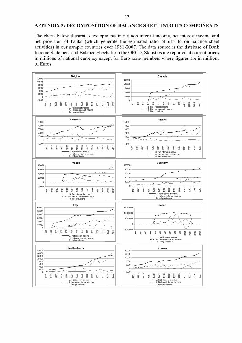
In order to provide a better understanding of factors underlying these developments, we

provide charts for the determinants of the ratio, namely net interest income, net non-interest

income and provisions on loans over the entire sample period (allowing for missing

observations) in Appendix 5. As would be expected, countries with the lowest average ratios

of OBS activity in general saw non-interest income falling short of net interest income.

However for countries having the highest ratios of OBS exposures, we observe non-interest

income growing faster than net interest income, specifically over 2001-2007, and in several

cases outstripping it. For example, in the UK over 2002-2007, non-interest income on average

grew by 14.7% per annum compared with 10% in 1996-2001, while net interest income

growth fell from 9% per annum in 1996-2001 to 6.2% in 2002-2007.

7

4 Estimation and results

As already noted above, the baseline for our analysis is the approach to crisis determination

set out in Barrell et al (2010). They used a panel multinomial logit approach with banking

crises as the dependent variable (see Appendix 7). As independent variables, they looked at

the role of unadjusted capital adequacy (LEV), bank’s narrow liquidity ratios (NLIQ), real

house price growth (RHPG) and the current balance as a percent of GDP (CBR) along with

the more traditionally used variables, GDP growth (YG), domestic credit growth (DCG), the

M2/FX reserves ratio (M2RES), inflation (INFL), real interest rates (RIR) and budget balance

to GDP ratio (BB) (see for example, Demirguc-Kunt and Detragiache, 1998, 2005). Barrell et

al found, however, that the traditional variables are not relevant for crisis determination in

OECD countries. Rather, the probability of banking crisis in 14 OECD countries can be

predicted by four “new” variables: two macroprudential indicators, banks’ unadjusted capital

adequacy and narrow liquidity and two real economy “vulnerability” variables, the change in

real residential property prices and the current account to GDP ratio. These had not been used

in previous work on banking crisis prediction because the bank variables and house prices are

typically not available for developing or emerging market countries.

These four crisis-prediction variables are in our view highly plausible and consistent as causes

of banking crises. The first two show how robust the banking system is to shocks, in terms of

capital and liquidity buffers. Meanwhile, the macroeconomic variables distinguish unbalanced

booms which are characterised by rapid growth in consumption and housing investment,

implying that supply fails to keep pace with respective demand. In such a context, the quality

of lending is likely to deteriorate, given lending assets the banks take on in such booms will

sharply deteriorate in the ensuing downturn. It is plausible that credit and GDP are unable to

distinguish crises as well as these variables since credit and output may also expand in a

situation of balanced growth where supply and demand balance is maintained both economy-

wide and in the property sector.

Although this model was shown to be extremely robust, a more comprehensive model would

encompass the risks generated by banks’ off-balance sheet positions. As previously noted,

capital adequacy and liquidity ratios may appear healthy in terms of on-balance sheet activity

but do not necessarily compensate for risky off-balance sheet activities. Therefore we add

variables that are intended to capture banks’ OBS activities as shown above, and use the

general to specific approach to arrive at the final specification of the equation. We check for

in-sample performance of the model and conduct a set of robustness tests to assess the

sensitivity of our results. We look at crises in 14 OECD countries over the period 1980 to

2008, with the choice of countries dictated by data availability in the OECD source.

We again use a multinomial logit method to regress a banking crisis variable (which is one for

the onset of the crisis and 0 otherwise) on the four variables cited in Barrell et al (2010)

together with all the “traditional” crisis determinants mentioned in the literature6 and

measures of banks’ OBS activity. Both the level of the ratio (defined as OFF TO ON) and the

change in the ratio (defined as D(OFF TO ON)) of off to on-balance sheet activities are used

as a proxy for off-balance sheet related risks. We employ the difference as well as the level

since the ratio on its own may not be enough to capture the trends developing in the banks’

OBS activities. Some countries with historically high off- to on-balance sheet ratios do not

necessarily have higher exposure to risk. On the other hand, those experiencing significant

6 Different results on the cuases or at least predictors of crises will imply different policy recommendations. For

example the negative result in Barrell et al (2010) for credit growth, and its lack of predictive power in Granger

causality tests between house price growth and credit growth casts doubt on the usefulness of reserving

cyclically against credit growth, as in Spain.

8

increases can be undergoing shifts in business strategies which expose them to new, untested

risks, with possible adverse selection, for example. This is consistent with what Davis (1995)

calls the “industrial organization” approach to financial instability, which suggests new entry

and structural change in financial markets is a key determinant of risk taking and hence of

crises.

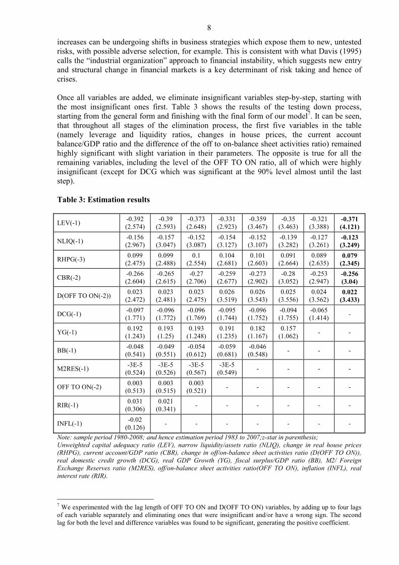
Once all variables are added, we eliminate insignificant variables step-by-step, starting with

the most insignificant ones first. Table 3 shows the results of the testing down process,

starting from the general form and finishing with the final form of our model7. It can be seen,

that throughout all stages of the elimination process, the first five variables in the table

(namely leverage and liquidity ratios, changes in house prices, the current account

balance/GDP ratio and the difference of the off to on-balance sheet activities ratio) remained

highly significant with slight variation in their parameters. The opposite is true for all the

remaining variables, including the level of the OFF TO ON ratio, all of which were highly

insignificant (except for DCG which was significant at the 90% level almost until the last

step).

Table 3: Estimation results

LEV(-1) -0.392

(2.574)

-0.39

(2.593)

-0.373

(2.648)

-0.331

(2.923)

-0.359

(3.467)

-0.35

(3.463)

-0.321

(3.388) -0.371

(4.121)

NLIQ(-1) -0.156

(2.967)

-0.157

(3.047)

-0.152

(3.087)

-0.154

(3.127)

-0.152

(3.107)

-0.139

(3.282)

-0.127

(3.261) -0.123

(3.249)

RHPG(-3) 0.099

(2.475)

0.099

(2.488)

0.1

(2.554)

0.104

(2.681)

0.101

(2.603)

0.091

(2.664)

0.089

(2.635) 0.079

(2.345)

CBR(-2) -0.266

(2.604)

-0.265

(2.615)

-0.27

(2.706)

-0.259

(2.677)

-0.273

(2.902)

-0.28

(3.052)

-0.253

(2.947) -0.256

(3.04)

D(OFF TO ON(-2)) 0.023

(2.472)

0.023

(2.481)

0.023

(2.475)

0.026

(3.519)

0.026

(3.543)

0.025

(3.556)

0.024

(3.562) 0.022

(3.433)

DCG(-1) -0.097

(1.771)

-0.096

(1.772)

-0.096

(1.769)

-0.095

(1.744)

-0.096

(1.752)

-0.094

(1.755)

-0.065

(1.414) -

YG(-1) 0.192

(1.243)

0.193

(1.25)

0.193

(1.248)

0.191

(1.235)

0.182

(1.167)

0.157

(1.062) - -

BB(-1) -0.048

(0.541)

-0.049

(0.551)

-0.054

(0.612)

-0.059

(0.681)

-0.046

(0.548) - - -

M2RES(-1) -3E-5

(0.524)

-3E-5

(0.526)

-3E-5

(0.567)

-3E-5

(0.549) - - - -

OFF TO ON(-2) 0.003

(0.513)

0.003

(0.515)

0.003

(0.521) - - - - -

RIR(-1) 0.031

(0.306)

0.021

(0.341) - - - - - -

INFL(-1) -0.02

(0.126) - - - - - - -

Note: sample period 1980-2008; and hence estimation period 1983 to 2007;z-stat in parenthesis; Unweighted capital adequacy ratio (LEV), narrow liquidity/assets ratio (NLIQ), change in real house prices

(RHPG), current account/GDP ratio (CBR), change in off/on-balance sheet activities ratio (D(OFF TO ON)),

real domestic credit growth (DCG), real GDP Growth (YG), fiscal surplus/GDP ratio (BB), M2/ Foreign

Exchange Reserves ratio (M2RES), off/on-balance sheet activities ratio(OFF TO ON), inflation (INFL), real

interest rate (RIR).

7 We experimented with the lag length of OFF TO ON and D(OFF TO ON) variables, by adding up to four lags

of each variable separately and eliminating ones that were insignificant and/or have a wrong sign. The second

lag for both the level and difference variables was found to be significant, generating the positive coefficient.

9

These results are in line with the findings of Barrell et al (2010), showing that in OECD

countries, asset price booms with an accompanying current account imbalance and lower

defences from less stringent bank regulation, are the most important factors driving the

probability of a banking crisis. And although lax monetary policy and credit booms may at

times contribute to banking crises, they are not the most powerful discriminators between

times of crisis onset and other periods in OECD countries.

As can be seen from Table 3, the change in the off/on-balance sheet activities ratio is

significant in addition to capital adequacy (LEV), the liquid asset ratio (NLIQ), the growth

rate of real house prices (RHPG) and the current account to GDP ratio (CBR). The variable

proxying changes in banks’ OBS activities has a positive effect on the probability of a crisis8,

hence, expansion of OBS activities relative to on-balance sheet assets by the banks increases

crisis probability.

We check for the in-sample performance of the final model and as shown in Table 4, the false

call rate when there is no crisis, known as the Type II error, is 26.5% and the false call rate

when there is a crisis, known as the Type I error is 20%, i.e. we only miss one in five crises.

The overall successful call rate (both crisis and no crisis called correctly) is 74%, with 16 out

of the 20 crisis episodes captured correctly at a cut-off point of 0.0559. Adding D(OFF TO

ON) improves the fit of the equation as compared to the version by Barrell et al (2010), as we

are able to capture correctly both more crises as well as non crisis periods (Appendix 3 lists

the estimation results together with the in-sample performance of the earlier model for

comparison).

Table 4: In-sample model performance

Dep=0 Dep=1 Total

P(Dep=1)<=0.055 253 4 257

P(Dep=1)>0.055 91 16 107

Total 344 20 364

Correct 253 16 269

% Correct 73.6 80.0 73.9

% Incorrect 26.5 20.0 26.1

Looking in more detail at the in-sample performance of the model (charts illustrating in-

sample probabilities for every country are presented in Appendix 6), all the systemic banking

crises are identified (see the crisis list in Appendix 7). Moreover, in the case of the four

missed crises (Italy 1990, UK 1995, Germany and Netherlands 2008) none can be considered

systemic. As for the so-called false alarms (Type II errors), more than half of them occur prior

to and/or after the crises onset, indicating that our model, on the top of identifying crisis, is

able to differentiate between periods of financial stability and instability very well.

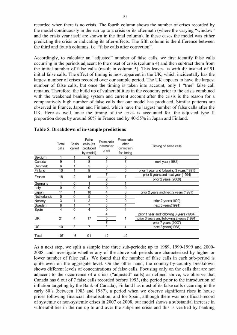
Table 5 analyses in-sample performance country by country. The first column shows the total

number of calls recorded by the model above the threshold value of 0.055. The next two

columns depict the number of crises called when there is a crisis, and the number of crises

8Table A1 in Appendix 3 show that these variables are not strongly correlated, suggesting that the change in

OBS is orthogonal to the other regressors in the equations, and hence multicollinearity and omitted variable bias

in our equations that omit this variable are not an issue. This is reinforced by the stable nature of parameters as

variables are dropped from the equation. 9 Calculated as the sample mean for onset of crises i.e. 20/364. We could of course use some other cut of point

for the crisis call, and this should depend on the weightings in the loss function for a false call when there is no

crisis to the loss from failing to call an actual crisis. If we wished to set a cut off to call all crises then we would

have around 282 false calls when there is no crisis.

10

recorded when there is no crisis. The fourth column shows the number of crises recorded by

the model continuously in the run up to a crisis or its aftermath (where the varying “window”

and the crisis year itself are shown in the final column). In these cases the model was either

predicting the crisis or indicating its after-effects. The fifth column is the difference between

the third and fourth columns, i.e. “false calls after correction”.

Accordingly, to calculate an “adjusted” number of false calls, we first identify false calls

occurring in the periods adjacent to the onset of crisis (column 4) and then subtract them from

the initial number of false calls (result in column 5). This leaves us with 49 instead of 91

initial false calls. The effect of timing is most apparent in the UK, which incidentally has the

largest number of crises recorded over our sample period. The UK appears to have the largest

number of false calls, but once the timing is taken into account, only 1 “true” false call

remains. Therefore, the build up of vulnerabilities in the economy prior to the crisis combined

with the weakened banking system and current account after the crisis is the reason for a

comparatively high number of false calls that our model has produced. Similar patterns are

observed in France, Japan and Finland, which have the largest number of false calls after the

UK. Here as well, once the timing of the crisis is accounted for, the adjusted type II

proportion drops by around 60% in France and by 40-55% in Japan and Finland.

Table 5: Breakdown of in-sample predictions

Belgium 1 1 0 0 0

Canada 9 1 8 1 7 next year (1983)

Denmark 6 1 5 0 5

Finland 10 1 9 4 5 prior 1 year and following 3 years(1991)

7 prior 6 years and next year (1994)

2 prior 2 years (2008)

Germany 1 0 1 0 1

Italy 0 0 0 0 0

Japan 11 1 10 4 6 prior 2 years and next 2 years (1991)

Netherlands 5 0 5 0 5

Norway 3 1 2 2 0 prior 2 years(1990)

Sweden 8 1 7 3 4 next 3 years(1991)

Spain 4 0 4 0 4

4 prior 1 year and following 3 years (1984)

5 prior 3 years and following 2 years (1991)

7 prior 7 years (2007)

US 10 3 7 3 4 next 3 years(1988)

Total 107 16 91 42 49

18 2 16

21 4 17

Timing of false calls

France

UK

7

1

Total

calls

Crisis

called

False

calls (as

produced

by model)

False calls

prior/after

crisis

False calls

after

correction

for timing

As a next step, we split a sample into three sub-periods; up to 1989, 1990-1999 and 2000-

2008, and investigate whether any of the above sub-periods are characterized by higher or

lower number of false calls. We found that the number of false calls in each sub-period is

quite even on the aggregate level. On the other hand, the country-by-country breakdown

shows different levels of concentrations of false calls. Focusing only on the calls that are not

adjacent to the occurrence of a crisis (“adjusted” calls) as defined above, we observe that

Canada has 6 out of 7 false calls recorded before 1993, (the period prior to the introduction of

inflation targeting by the Bank of Canada); Finland has most of its false calls occurring in the

early 80’s (between 1983 and 1987), a period when we observe significant rises in house

prices following financial liberalisation; and for Spain, although there was no official record

of systemic or non-systemic crises in 2007 or 2008, our model shows a substantial increase in

vulnerabilities in the run up to and over the subprime crisis and this is verified by banking

11

difficulties in that country which are now coming to light (see for example Financial Times

(2010)). Therefore, it appears that the vast majority of false calls reported by the model are

associated with periods of risk accumulation in the economies or with periods of weakened

economic conditions in the aftermath of crises.

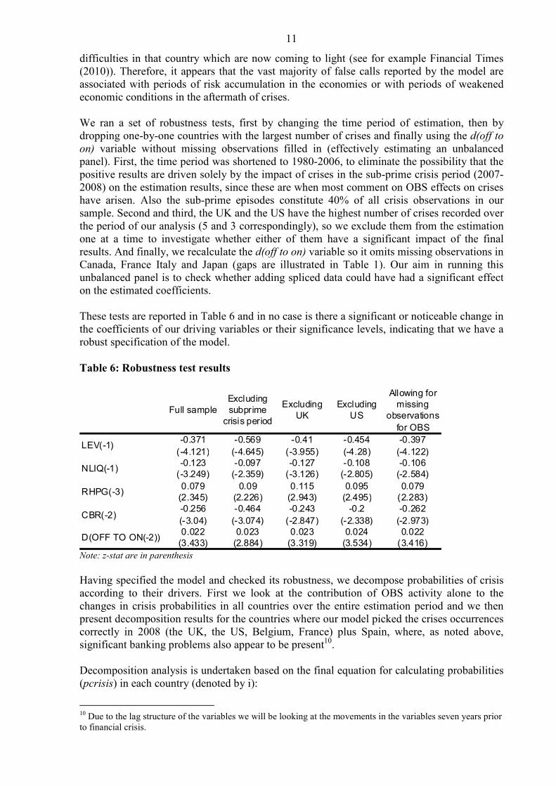
We ran a set of robustness tests, first by changing the time period of estimation, then by

dropping one-by-one countries with the largest number of crises and finally using the d(off to

on) variable without missing observations filled in (effectively estimating an unbalanced

panel). First, the time period was shortened to 1980-2006, to eliminate the possibility that the

positive results are driven solely by the impact of crises in the sub-prime crisis period (2007-

2008) on the estimation results, since these are when most comment on OBS effects on crises

have arisen. Also the sub-prime episodes constitute 40% of all crisis observations in our

sample. Second and third, the UK and the US have the highest number of crises recorded over

the period of our analysis (5 and 3 correspondingly), so we exclude them from the estimation

one at a time to investigate whether either of them have a significant impact of the final

results. And finally, we recalculate the d(off to on) variable so it omits missing observations in

Canada, France Italy and Japan (gaps are illustrated in Table 1). Our aim in running this

unbalanced panel is to check whether adding spliced data could have had a significant effect

on the estimated coefficients.

These tests are reported in Table 6 and in no case is there a significant or noticeable change in

the coefficients of our driving variables or their significance levels, indicating that we have a

robust specification of the model.

Table 6: Robustness test results

LEV(-1)-0.371

(-4.121)

-0.569

(-4.645)

-0.41

(-3.955)

-0.454

(-4.28)

-0.397

(-4.122)

NLIQ(-1)-0.123

(-3.249)

-0.097

(-2.359)

-0.127

(-3.126)

-0.108

(-2.805)

-0.106

(-2.584)

RHPG(-3)0.079

(2.345)

0.09

(2.226)

0.115

(2.943)

0.095

(2.495)

0.079

(2.283)

CBR(-2)-0.256

(-3.04)

-0.464

(-3.074)

-0.243

(-2.847)

-0.2

(-2.338)

-0.262

(-2.973)

D(OFF TO ON(-2))0.022

(3.433)

0.023

(2.884)

0.023

(3.319)

0.024

(3.534)

0.022

(3.416)

Allowing for

missing

observations

for OBS

Full sample

Excluding

subprime

crisis period

Excluding

UK

Excluding

US

Note: z-stat are in parenthesis

Having specified the model and checked its robustness, we decompose probabilities of crisis

according to their drivers. First we look at the contribution of OBS activity alone to the

changes in crisis probabilities in all countries over the entire estimation period and we then

present decomposition results for the countries where our model picked the crises occurrences

correctly in 2008 (the UK, the US, Belgium, France) plus Spain, where, as noted above,

significant banking problems also appear to be present10

.

Decomposition analysis is undertaken based on the final equation for calculating probabilities

(pcrisis) in each country (denoted by i):

10

Due to the lag structure of the variables we will be looking at the movements in the variables seven years prior

to financial crisis.

12

( )2,2,3,1,1, 02.026.008.012.037.0,1

1−−−−− +−+−−−

+=

titittiti dofftooncbrrphgnliqlevtie

pcrisis (3)

The contribution of each variable to the change in the probability between the adjacent years

is calculated by subtracting the probability generated based on the final lag structure of all

variables apart from one (which is taken with extra lag) from the probability with lag structure

of variables based on the final specification. These are described in the literature as the time

specific marginal effects of each of the variables. The example below, where subscripts i,l,t

denote country, variable (which is taken with extra lag) and time period correspondingly,

illustrates how the contribution of unadjusted capital adequacy (LEV) is calculated:

( )

( )2,2,3,1,2,

2,2,3,1,1,

02.024.008.012.037.0

02.026.008.012.037.0

1,,,

1

1

1

1

−−−−−

−−−−−

+−+−−−

+−+−−−

−

+−

+

=−

tititititi

tititititi

dofftooncbrrphgnliqlev

dofftooncbrrphgnliqlev

tliti

e

e

pcrisispcrisis

(4)

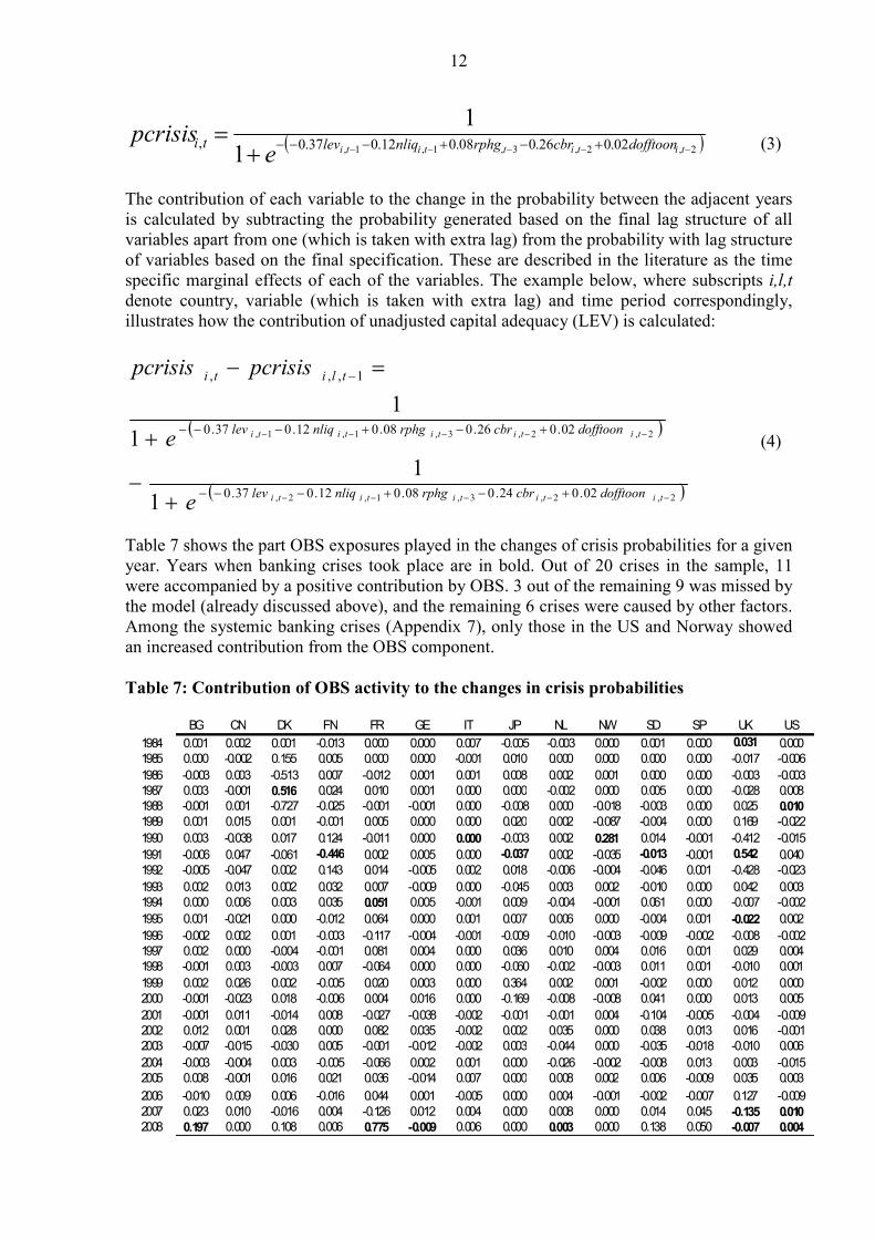
Table 7 shows the part OBS exposures played in the changes of crisis probabilities for a given

year. Years when banking crises took place are in bold. Out of 20 crises in the sample, 11

were accompanied by a positive contribution by OBS. 3 out of the remaining 9 was missed by

the model (already discussed above), and the remaining 6 crises were caused by other factors.

Among the systemic banking crises (Appendix 7), only those in the US and Norway showed

an increased contribution from the OBS component.

Table 7: Contribution of OBS activity to the changes in crisis probabilities

BG CN DK FN FR GE IT JP NL NW SD SP UK US

1984 0.001 0.002 0.001 -0.013 0.000 0.000 0.007 -0.005 -0.003 0.000 0.001 0.000 0.031 0.000

1985 0.000 -0.002 0.155 0.005 0.000 0.000 -0.001 0.010 0.000 0.000 0.000 0.000 -0.017 -0.006

1986 -0.003 0.003 -0.513 0.007 -0.012 0.001 0.001 0.008 0.002 0.001 0.000 0.000 -0.003 -0.003

1987 0.003 -0.001 0.516 0.024 0.010 0.001 0.000 0.000 -0.002 0.000 0.005 0.000 -0.028 0.008

1988 -0.001 0.001 -0.727 -0.025 -0.001 -0.001 0.000 -0.008 0.000 -0.018 -0.003 0.000 0.025 0.010

1989 0.001 0.015 0.001 -0.001 0.005 0.000 0.000 0.020 0.002 -0.087 -0.004 0.000 0.169 -0.022

1990 0.003 -0.038 0.017 0.124 -0.011 0.000 0.000 -0.003 0.002 0.281 0.014 -0.001 -0.412 -0.015

1991 -0.006 0.047 -0.061 -0.446 0.002 0.005 0.000 -0.037 0.002 -0.035 -0.013 -0.001 0.542 0.040

1992 -0.005 -0.047 0.002 0.143 0.014 -0.005 0.002 0.018 -0.006 -0.004 -0.046 0.001 -0.428 -0.023

1993 0.002 0.013 0.002 0.032 0.007 -0.009 0.000 -0.045 0.003 0.002 -0.010 0.000 0.042 0.003

1994 0.000 0.006 0.003 0.035 0.051 0.005 -0.001 0.009 -0.004 -0.001 0.061 0.000 -0.007 -0.002

1995 0.001 -0.021 0.000 -0.012 0.064 0.000 0.001 0.007 0.006 0.000 -0.004 0.001 -0.022 0.002

1996 -0.002 0.002 0.001 -0.003 -0.117 -0.004 -0.001 -0.009 -0.010 -0.003 -0.009 -0.002 -0.008 -0.002

1997 0.002 0.000 -0.004 -0.001 0.081 0.004 0.000 0.036 0.010 0.004 0.016 0.001 0.029 0.004

1998 -0.001 0.003 -0.003 0.007 -0.064 0.000 0.000 -0.060 -0.002 -0.003 0.011 0.001 -0.010 0.001

1999 0.002 0.026 0.002 -0.005 0.020 0.003 0.000 0.364 0.002 0.001 -0.002 0.000 0.012 0.000

2000 -0.001 -0.023 0.018 -0.006 0.004 0.016 0.000 -0.169 -0.008 -0.008 0.041 0.000 0.013 0.005

2001 -0.001 0.011 -0.014 0.008 -0.027 -0.038 -0.002 -0.001 -0.001 0.004 -0.104 -0.005 -0.004 -0.009

2002 0.012 0.001 0.028 0.000 0.082 0.035 -0.002 0.002 0.035 0.000 0.038 0.013 0.016 -0.001

2003 -0.007 -0.015 -0.030 0.005 -0.001 -0.012 -0.002 0.003 -0.044 0.000 -0.035 -0.018 -0.010 0.006

2004 -0.003 -0.004 0.003 -0.005 -0.066 0.002 0.001 0.000 -0.026 -0.002 -0.008 0.013 0.003 -0.015

2005 0.008 -0.001 0.016 0.021 0.036 -0.014 0.007 0.000 0.008 0.002 0.006 -0.009 0.035 0.003

2006 -0.010 0.009 0.006 -0.016 0.044 0.001 -0.005 0.000 0.004 -0.001 -0.002 -0.007 0.127 -0.009

2007 0.023 0.010 -0.016 0.004 -0.126 0.012 0.004 0.000 0.008 0.000 0.014 0.045 -0.135 0.0102008 0.197 0.000 0.108 0.006 0.775 -0.009 0.006 0.000 0.003 0.000 0.138 0.050 -0.007 0.004

13

Similar calculations were undertaken for the other four remaining variables. As the

relationship is not linear, the sum of all contributions from the right hand side variables are

not exactly equal to the change in the dependent variable. The remaining term accounts for

the interaction between the independent variables, which can be computed by summing two

or three individual marginal contributions and comparing that to a marginal contribution

where two or three of the driving variables are allowed to vary. We call the sum of these

terms the adjustment (Adj) for interaction and add it to the direct contributions of the right

hand side variables. The cumulative change in the probability and its contributing variables

over a certain time period is just a sum of the changes in the probabilities and the sum of

contributions by each variable over the same time span.

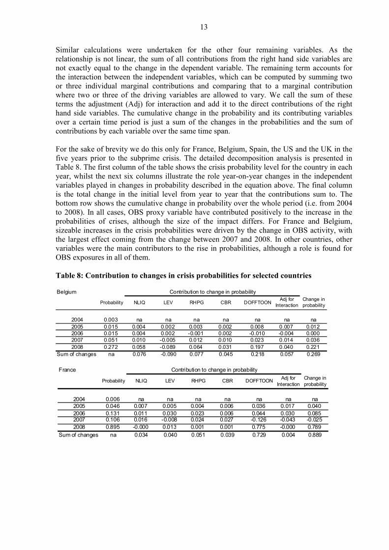
For the sake of brevity we do this only for France, Belgium, Spain, the US and the UK in the

five years prior to the subprime crisis. The detailed decomposition analysis is presented in

Table 8. The first column of the table shows the crisis probability level for the country in each

year, whilst the next six columns illustrate the role year-on-year changes in the independent

variables played in changes in probability described in the equation above. The final column

is the total change in the initial level from year to year that the contributions sum to. The

bottom row shows the cumulative change in probability over the whole period (i.e. from 2004

to 2008). In all cases, OBS proxy variable have contributed positively to the increase in the

probabilities of crises, although the size of the impact differs. For France and Belgium,

sizeable increases in the crisis probabilities were driven by the change in OBS activity, with

the largest effect coming from the change between 2007 and 2008. In other countries, other

variables were the main contributors to the rise in probabilities, although a role is found for

OBS exposures in all of them.

Table 8: Contribution to changes in crisis probabilities for selected countries

Belgium

2004 0.003 na na na na na na na

2005 0.015 0.004 0.002 0.003 0.002 0.008 0.007 0.012

2006 0.015 0.004 0.002 -0.001 0.002 -0.010 -0.004 0.000

2007 0.051 0.010 -0.005 0.012 0.010 0.023 0.014 0.036

2008 0.272 0.058 -0.089 0.064 0.031 0.197 0.040 0.221

Sum of changes na 0.076 -0.090 0.077 0.045 0.218 0.057 0.269

Probability NLIQ LEV RHPG CBR DOFFTOONAdj for

Interaction

Change in

probability

Contribution to change in probability

France


2005 0.046 0.007 0.005 0.004 0.006 0.036 0.017 0.040

2006 0.131 0.011 0.030 0.023 0.006 0.044 0.030 0.0852007 0.106 0.016 -0.008 0.024 0.027 -0.126 -0.043 -0.025

2008 0.895 -0.000 0.013 0.001 0.001 0.775 -0.000 0.789

Sum of changes na 0.034 0.040 0.051 0.039 0.729 0.004 0.889

Probability NLIQ CBR DOFFTOONChange in

probability


Adj for

InteractionLEV RHPG

14

Spain


2005 0.067 0.022 -0.012 0.026 0.004 -0.009 -0.001 0.032

2006 0.173 0.031 0.040 0.017 0.055 -0.007 0.030 0.1062007 0.398 0.065 0.044 -0.013 0.120 0.045 0.037 0.225

2008 0.479 -0.021 0.016 -0.063 0.098 0.050 -0.001 0.081

Sum of changes na 0.097 0.089 -0.033 0.277 0.079 0.064 0.444

Change in

probability


Probability NLIQ LEV RHPG CBR DOFFTOONAdj for

Interaction

UK


2005 0.241 0.002 0.010 0.099 -0.007 0.035 0.015 0.125

2006 0.442 0.009 0.057 -0.008 0.031 0.127 0.016 0.201

2007 0.292 -0.002 0.024 -0.066 0.026 -0.135 -0.003 -0.151

2008 0.253 0.010 0.026 -0.119 0.036 -0.007 -0.015 -0.038

Sum of changes na 0.020 0.118 -0.094 0.087 0.020 0.013 0.137

RHPG CBR


Probability NLIQ LEVAdj for

Interaction

Change in

probabilityDOFFTOON

US


2005 0.045 -0.017 -0.015 -0.002 0.004 0.003 0.001 -0.029

2006 0.043 0.002 -0.000 -0.002 0.006 -0.009 -0.001 -0.002

2007 0.064 0.002 -0.008 0.011 0.008 0.010 0.002 0.021

2008 0.087 0.004 0.004 0.010 0.002 0.004 0.002 0.023

Sum of changes na -0.008 -0.019 0.017 0.019 0.008 0.004 0.013

Probability NLIQ LEV RHPG CBRAdj for

Interaction

Change in

probability


DOFFTOON

5 Policy Implications

In assessing OBS activity and the appropriate regulatory response, it should first be

acknowledged that off-balance sheet activity can be productive, it can spread risks and fill

holes in the market, in effect bringing the economy closer to Arrow-Debreu optimum by

creating a wider range of contingent markets. These should increase welfare and increase

output. However, it was clear in the recent crisis that structures became too complex and risks

too opaque, and regulators found it difficult to set up defences against the systemic risks

involved. Accordingly, policy action is required.

The results have direct implications for macroprudential policy, since they suggest that

changes in the OBS ratio have a major impact on the likelihood of a systemic crisis. In order

to offset this, the authorities can either directly target the required ratios of off- to on-balance

sheet activities, implying direct limits on banks’ activities at micro level11

, or increase capital

and/or liquidity requirements for banks at macro level, thus counteracting and dampening

amplified risk exposure from elevated levels of OBS activity. Both of these approaches would

require significantly better monitoring of OBS, and regulatory changes would be necessary to

ensure this, which we discuss in the following paragraphs.

It is important that there is international agreement on regulation of OBS to prevent

‘competition in laxity’ and ensure a level playing field. The Bank for International Standards

(BIS) and the Basel Agreements are meant to achieve this. However, this requires the

cooperation of all major parties and a commitment to common goals. In this context, an

11

To give an idea of the magnitudes concerned, we present in Appendix 8 calculations of required changes in the

OBS proxy to ensure crisis probabilities in each country and in each year in our sample do not exceed the sample

average.

15

interesting sideline to our research is the difficulty of detecting banking crises in 2007-8 in

Germany and the Netherlands with our model. One aspect of the difficulties in those countries

is that the banks purchased large quantities of securitized US assets, some of which were held

on balance sheet and some in SIVs and conduits. There were no other indications of financial

risk in those countries such as house price booms, balance of payments deficits or capital or

liquidity shortages as measured, and that is why the model fails to detect the risk. This

underlines the need for accurate measurement of OBS at a global as well as a national level

and also for international cooperation of (in this case) the US authorities in communicating

their assessment of risks on these instruments to cross border banks which are exposed to the

related risks.

There are a number of options that have to be considered as further regulatory responses to

the problems we have seen related to OBS activity, which is of course highly diverse. One

would involve changes to the (mainly US) model of separating the origination and the

distribution of assets. If the originator of a loan has no stake in its risks once it is sold on, then

there is less incentive to properly evaluate the risk. There may be a need to ensure that a

significant proportion of the securities are retained by the originator (“skin in the game”). Or

alternatively, residual obligations could be written into change of ownership contracts, and

this could be enforced.

Other proposals to reduce the scale of OBS activity involve taxes on credit and taxes on

transactions. These are two different issues, and they are designed to address two different

problems. Taxes on credit would reduce level of borrowing by individuals, but not necessarily

affect the cyclicity of asset prices, and that would be essential. Hence although there is no

reason why taxes on credit should not be used to raise revenue it is not clear that they will

reduce the risks of crises. The same might be said of transactions taxes and bank taxes

designed to contribute to a fund to cover future costs. Indeed, there is evidence that such

schemes increase the risk of crises, as they are similar to deposit insurance, and its impact on

crisis probabilities is clear in the literature. Perhaps the only sound reason for taxing

transactions (apart from revenue) is to make sure that there is a proper record, and this could

be achieved by requiring recourse loans were all registered (if you do not register, you cannot

enforce the loan).

Clearing houses and registers serve the same purpose, as recording and understanding

contracts is also essential to regulating markets. OBS have been underestimated in part

because there was no register of such activities, and especially a chronic dearth of information

on over-the-counter (OTC) trades. Creating central counterparties, or clearing houses for off-

balance sheet activities and in particular for OTCs would be a very effective way of ensuring

regulators could respond, and to the extent it involves transactions costs it would reduce the

scale of such activities (IMF 2009).

In this context, as a specific macroprudential instrument, Barrell and Weale (2010) suggest

stamp duties on all OBS trades as a way of recording them, and Singh (2010) has suggested

there could be a tax based on over-the-counter payables in derivative markets. It would be

based on off-balance-sheet data, including netted exposures, thus measuring the potential

systemic interconnectedness of these contracts more accurately. On the other hand as pointed

out by IMF (2010), the tax would only be based on banks’ OTC derivative payables. It does

not increase institutions’ capital base, nor would it take into account second-round contagion

effects.

On balance, overall, financial regulations are changing in response to the crisis, and the core

problems behind the current crisis seem likely to be addressed, with the scale and complexity

16

of OBS financial products almost certainly being restricted. Of course other problems may

emerge and financial innovations may get round new regulations, as Goodhart (2008)

discusses. Hence the need for continuous monitoring and adaptation of regulation of banks

and financial markets.

6 Conclusions

We have estimated the off-balance sheet exposures of the banking systems by employing the

ratio of off- to on-balance sheet activities in an econometric model of crisis determination. We

checked for the significance of both the ratio and the change in the ratio of off- to on-balance

sheet activities and found that along with capital, liquidity, property price growth and current

account deficits, changes in the off- to on-balance sheet activities ratio has a positive and

significant effect on the probability of a banking crisis. The inclusion of such a proxy variable

for banks’ OBS activity in the estimation improved in-sample performance of the model, with

more crisis periods being captured and the number of false calls reduced. 80% of crises were

captured and once the timing of the false calls was accounted for, the number of false calls

dropped from 26.5% to 14%. We ran several robustness tests and we conclude that the model

is well specified.

Decomposition analysis looking at the driving factors behind the change in probabilities from

year to year reveals that, out of 20 crises in the sample 11 were accompanied by increases in

OBS activity. At the same time, in all countries where our model has flagged the crisis

correctly in 2008, the OBS proxy variables have contributed positively to the increase in the

probabilities of banking crises.

Regulation needs to respond to the risks posed by OBS activities, with controls needed at a

macroprudential as well as a microprudential level. Reducing the scale and complexity of

OBS activity may be essential, and there are several ways to do this. Registers and clearing

houses may make OBS activity more transparent and easier to provision against. And

requiring mandatory holdings or recourse on securitized assets may also be beneficial. Taxes

on OTC derivatives might also be considered.

Overall our findings can be considered as a step towards quantifying the effect OBS activity

has on the occurrence of a crisis. Further investigation in this area can be conducted once

more detailed data are available, which will allow researchers to adjust banks liquidity and

leverage ratios for the size of the OBS exposures directly and test for impact on crisis

probabilities more precisely. Given how essential such calculations are, we would suggest

direct regulatory action (to produce that data) would be wise.

17

References

Acharya, V. and Richardson, M. (2009), “Causes of the Financial Crisis”, Critical Review,

Vol. 21, Issue 2 & 3, pages 195 – 210, June 2009.

Barrell R, Davis P, Karim D and Liadze I (2010), “The impact of global imbalances: does the

current account balance help to predict banking crises in OECD countries?”, NIESR

Working Paper No 351

Barrell, R., Weale, M. (2010), “Fiscal Policy, Fairness between Generations and National

Saving”, NIESR Working Paper No. 338

Borio C and Drehmann M (2009) “Assessing the risk of banking crises - revisited”, BIS

Quarterly Review, March, pp 29-46.

Boyd, John H. and Gertler, Mark (1994), "Are Banks Dead? Or are the Reports Greatly

Exaggerated?," Quarterly Review, Federal Reserve Bank of Minneapolis, Issue

Summer, pages 2-23.

Breusch, T.S., and A. R. Pagan (1980). “The Lagrange Multiplier test and its application to

model specifications in econometrics", Review of Economic Studies 47, 239-53.

Davis E P (1995), “Debt, Financial Fragility, and Systemic Risk”, Oxford University Press

Davis E P (2009), "Financial Stability in the United Kingdom: Banking on Prudence" OECD

Economics Department Working Paper no. 717

Davis E P, Fic T and Karim D (2010), “Tier 2 capital and bank behaviour”, mimeo, NIESR

Davis E P and Tuori K (2000), "The changing structure of banks' income - An Empirical

Investigation", Working Paper No. 00-11, Brunel University, West London

De Bandt O and Davis E P (2000), "Competition, contestability and market structure in

European banking sectors on the eve of EMU", Journal of Banking and Finance, 24,

1045-1066

Demirgüc-Kunt, A., and Detragiache, E., 1998. The determinants of banking crises in

developed and developing countries. IMF Staff Papers, 45, 81-109.

Demirgüç-Kunt, A and Detragiache, E (2005). "Cross-Country Empirical Studies of Systemic

Bank Distress: A Survey.", IMF Working Papers 05/96, International Monetary Fund.

Farhi, E. and Tirole, J. (2009), `Collective Moral Hazard, Maturity Mismatch and Systemic

Bailouts'. NBER Working Paper, No. 15138. (July 2009).

Feldman R and Lueck M (2007), “Are banks really dying this time?” The Region, Federal

Reserve Bank of Minneapolis, September 2007, 6-9, 42-51.

Financial Times (2010), “Madrid turmoil sparks fear of crisis spending”, FT, 15th

June 2010

Goodhart, C.A.E. (2008), ‘The boundary problem in financial regulation’, National Institute

Economic Review, 206, October, pp. 48–55.

IMF (2009), Global Financial Stability Report; Navigating the Financial Challenges Ahead,

Washington D.C., October.

IMF (2010), Global Financial Stability Report; Meeting New Challenges to Stability and

Building a Safer System, Washington D.C., April.

Laeven, L., and Valencia, F., (2007), Systemic banking crises: A new database. IMF Working

Paper No. WP/08/224

Rogers, K (1998), `Nontraditional Activities and the Efficiency of US Commercial Banks'.

Journal of Banking & Finance, Vol. 22, Issue 4, pages 467-482.

Singh, Manmohan, 2010, “Collateral, Netting and Systemic Risk in the OTC Derivatives

Market,” IMF Working Paper 10/99 (Washington: International Monetary Fund).

World Bank (2003), “Banking crisis dataset”, World Bank, Washington DC

18

APPENDIX 1

Data Issues in Using Bankscope

In order to obtain country-level measures, the user has to aggregate the OBS series for

individual banks within a country. This requires a judgment on the shareholder criteria used

for the aggregation: for example, we opted to include all banks in an economy where at least

50% of the shares were owned domestically. This excluded banks with majority foreign

ownership but which may have held significant amounts of OBS exposures within the

domestic system.

The aggregated data for each country showed major time series problems:

1. Bankscope only allowed us to access data back to 2001 which meant the OBS

series were shorter than the remaining sample period (1980 – 2007). This meant

we had to make the crude assumption that OBS activity prior to 2001 had

remained stable in each country in order to fill the missing observations.12

2. Even when Bankscope covered the years, many individual observations of OBS

within each series were missing. Due to points (3) and (4) below, it was impossible

to replace such missing observations with reliable alternative data points.

3. Bankscope’s OBS assets series prior to 2004 are particularly patchy in their

coverage with countries such as Finland having far fewer observations than others

(such as Germany, Denmark and the USA).

4. We construct the off-balance sheet exposures for a banking system by aggregating

the figures for all banks that comprise the top 80% of total banking system assets.

The problem with Bankscope data is that the banks that comprise the top 80% with

OBS data vary vastly from year to year. For example, in France in 2004, Credit

Agricole SA was the largest bank in terms of assets, yet this bank does not

contribute to the top 80% of assets in 2002; the bank only starts reporting in 2004.

Thereon, Credit Agricole forms a large part of the French off-balance sheet

exposures. Such anomalies make the Bankscope data extremely volatile at best and

unreliable at worst.

Data Issues in Using the: OECD Bank Income and Balance Sheet Dataset

1. The UK does not report data to the OECD prior to 1984, although from there on, figures

are available till 2007. Because the FSA were able to provide us with consistent series

for the entire sample period, we opted to use their data for the UK. The FSA data

covered all large UK commercial banks and were compatible with the OECD figures we

could access.

2. The OECD data for Japan are missing from 2004 onwards. It is possible to substitute the

missing observations with data from the Japanese Banker’s Association but there remain

difficulties with obtaining consistent estimates of non-interest income from the two

sources.

3. Belgium, Canada, France, Italy and Japan do not report some series around the

beginning of our sample period. For these countries, we were able to obtain missing

observations by splicing from old copies of OECD Bank Profitability Statistical

Supplements. However, we are unable to confirm whether the aggregation methods of

the OECD are consistent across their data sources.

Missing observations for 1980 were constructed by applying average growth for 3 preceding

years to the data in 1981.

12

This does not of course nullify the major benefits of Bankscope for undertaking cross sectional and panel

research for individual banks (see Davis et al (2010) for example).

19

APPENDIX 2: METHODOLOGY FOR CALCULATING A PROXY FOR OFF-

BALANCE SHEET ACTIVITY

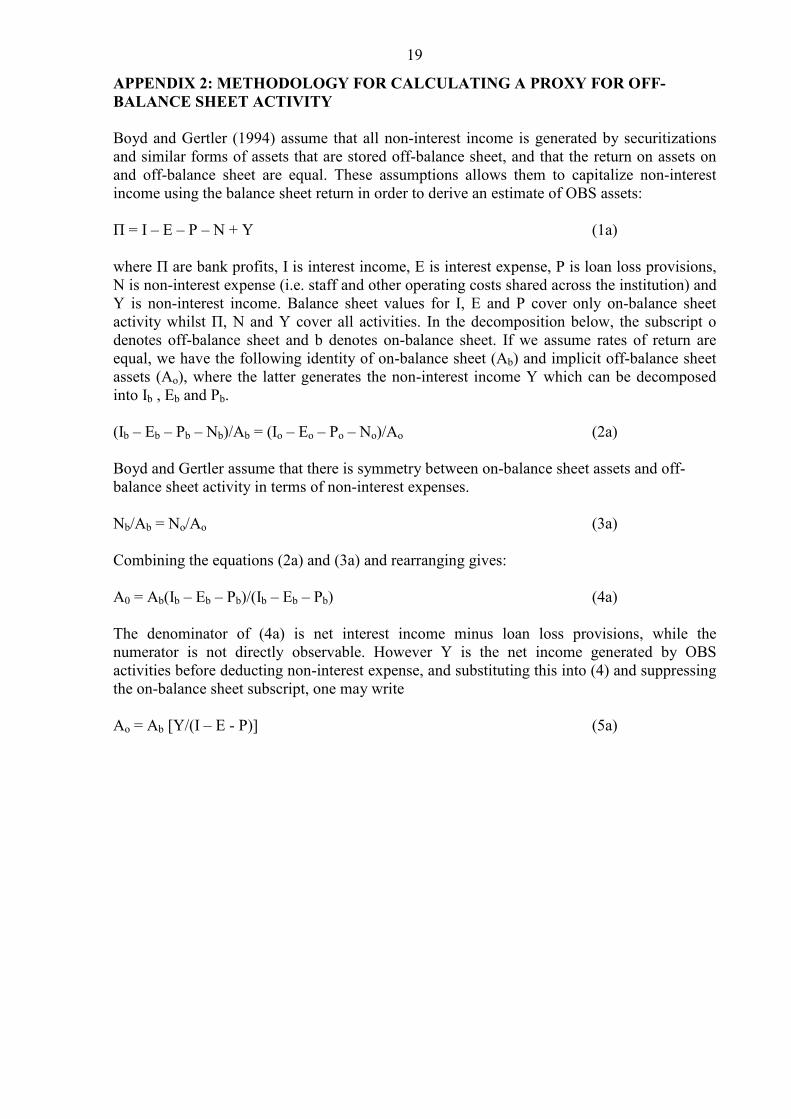
Boyd and Gertler (1994) assume that all non-interest income is generated by securitizations

and similar forms of assets that are stored off-balance sheet, and that the return on assets on

and off-balance sheet are equal. These assumptions allows them to capitalize non-interest

income using the balance sheet return in order to derive an estimate of OBS assets:

Π = I – E – P – N + Y (1a)

where Π are bank profits, I is interest income, E is interest expense, P is loan loss provisions,

N is non-interest expense (i.e. staff and other operating costs shared across the institution) and

Y is non-interest income. Balance sheet values for I, E and P cover only on-balance sheet

activity whilst Π, N and Y cover all activities. In the decomposition below, the subscript o

denotes off-balance sheet and b denotes on-balance sheet. If we assume rates of return are

equal, we have the following identity of on-balance sheet (Ab) and implicit off-balance sheet

assets (Ao), where the latter generates the non-interest income Y which can be decomposed

into Ib , Eb and Pb.

(Ib – Eb – Pb – Nb)/Ab = (Io – Eo – Po – No)/Ao (2a)

Boyd and Gertler assume that there is symmetry between on-balance sheet assets and off-

balance sheet activity in terms of non-interest expenses.

Nb/Ab = No/Ao (3a)

Combining the equations (2a) and (3a) and rearranging gives:

A0 = Ab(Ib – Eb – Pb)/(Ib – Eb – Pb) (4a)

The denominator of (4a) is net interest income minus loan loss provisions, while the

numerator is not directly observable. However Y is the net income generated by OBS

activities before deducting non-interest expense, and substituting this into (4) and suppressing

the on-balance sheet subscript, one may write

Ao = Ab [Y/(I – E - P)] (5a)

20

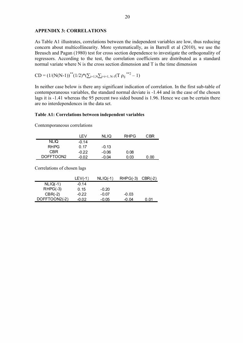
APPENDIX 3: CORRELATIONS

As Table A1 illustrates, correlations between the independent variables are low, thus reducing

concern about multicollinearity. More systematically, as in Barrell et al (2010), we use the

Breusch and Pagan (1980) test for cross section dependence to investigate the orthogonality of

regressors. According to the test, the correlation coefficients are distributed as a standard

normal variate where N is the cross section dimension and T is the time dimension

CD = (1/(N(N-1))**

(1/2)*(∑i=1,N∑j=i+1, N-1(T ρij **2

– 1)

In neither case below is there any significant indication of correlation. In the first sub-table of

contemporaneous variables, the standard normal deviate is -1.44 and in the case of the chosen

lags it is -1.41 whereas the 95 percent two sided bound is 1.96. Hence we can be certain there

are no interdependences in the data set.

Table A1: Correlations between independent variables

Contemporaneous correlations

LEV NLIQ RHPG CBR

NLIQ -0.14

RHPG 0.17 -0.13

CBR -0.22 -0.06 0.08DOFFTOON2 -0.02 -0.04 0.03 0.00

Correlations of chosen lags

LEV(-1) NLIQ(-1) RHPG(-3) CBR(-2)

NLIQ(-1) -0.14

RHPG(-3) 0.15 -0.20

CBR(-2) -0.22 -0.07 -0.03

DOFFTOON2(-2) -0.02 -0.05 -0.04 0.01

21

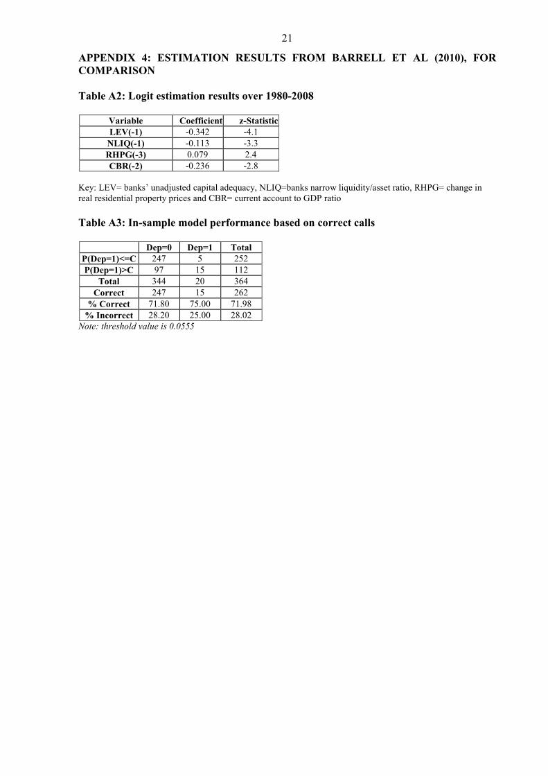
APPENDIX 4: ESTIMATION RESULTS FROM BARRELL ET AL (2010), FOR

COMPARISON

Table A2: Logit estimation results over 1980-2008

Variable Coefficient z-Statistic

LEV(-1) -0.342 -4.1

NLIQ(-1) -0.113 -3.3

RHPG(-3) 0.079 2.4

CBR(-2) -0.236 -2.8

Key: LEV= banks’ unadjusted capital adequacy, NLIQ=banks narrow liquidity/asset ratio, RHPG= change in

real residential property prices and CBR= current account to GDP ratio

Table A3: In-sample model performance based on correct calls

Dep=0 Dep=1 Total

P(Dep=1)<=C 247 5 252

P(Dep=1)>C 97 15 112

Total 344 20 364

Correct 247 15 262

% Correct 71.80 75.00 71.98

% Incorrect 28.20 25.00 28.02

Note: threshold value is 0.0555

22

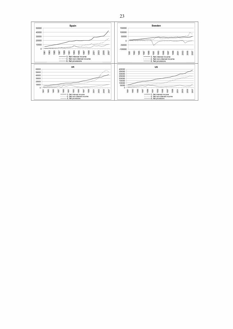
APPENDIX 5: DECOMPOSITION OF BALANCE SHEET INTO ITS COMPONENTS

The charts below illustrate developments in net non-interest income, net interest income and

net provision of banks (which generate the estimated ratio of off- to on balance sheet

activities) in our sample countries over 1981-2007. The data source is the database of Bank

Income Statement and Balance Sheets from the OECD. Statistics are reported at current prices

in millions of national currency except for Euro zone members where figures are in millions

of Euros.

Belgium

-2000

0

2000

4000

6000

8000

10000

12000

1981

1983

1985

1987

1989

1991

1993

1995

1997

1999

2001

2003

2005

2007

3. Net interest income 4. Net non-interest income8. Net provisions

Canada

0

10000

20000

30000

40000

50000

1981

1983

1985

1987

1989

1991

1993

1995

1997

1999

2001

2003

2005

2007


Denmark

-10000

0

10000

20000

30000

40000

50000

1981

1983

1985

1987

1989

1991

1993

1995

1997

1999

2001

2003

2005

2007


Finland

-1000

0

1000

2000

3000

4000

5000

1981

1983

1985

1987

1989

1991

1993

1995

1997

1999

2001

2003

2005

2007


France

-20000

0

20000

40000

60000

80000

1981

1983

1985

1987

1989

1991

1993

1995

1997

1999

2001

2003

2005

2007


Germany

0

20000

40000

60000

80000

100000

1981

1983

1985

1987

1989

1991

1993

1995

1997

1999

2001

2003

2005

2007


Italy

0

10000

20000

30000

40000

50000

60000

1981

1983

1985

1987

1989

1991

1993

1995

1997

1999

2001

2003

2005

2007


Japan

-5000000

0

5000000

10000000

15000000

1981

1983

1985

1987

1989

1991

1993

1995

1997

1999

2001

2003

2005

2007


Neetherlands

0

5000

10000

1500020000

25000

30000

35000

40000

1981

1983

1985

1987

1989

1991

1993

1995

1997

1999

2001

2003

2005

2007


Norway

-10000

0

10000

20000

30000

40000

50000

1981

1983

1985

1987

1989

1991

1993

1995

1997

1999

2001

2003

2005

2007


23

Spain

0

10000

20000

30000

40000

50000

1981

1983

1985

1987

1989

1991

1993

1995

1997

1999

2001

2003

2005

2007


Sweden

-100000

-50000

0

50000

100000

150000

1981

1983

1985

1987

1989

1991

1993

1995

1997

1999

2001

2003

2005

2007


UK

0

10000

20000

30000

40000

50000

60000

1981

1983

1985

1987

1989

1991

1993

1995

1997

1999

2001

2003

2005

2007


US

050000

100000

150000200000

250000300000

350000

400000

1981

1983

1985

1987

1989

1991

1993

1995

1997

1999

2001

2003

2005

2007


24

APPENDIX 6: IN-SAMPLE PROBABILITIES

The charts below illustrate in-sample probabilities of crises based on final estimation results

for all countries in our sample (solid line depicts probabilities and the dashed line indicates

the threshold value of 0.055).

0.0

0.2

0.4

0.6

0.8

1.0

1983

1985

1987

1989

1991

1993

1995

1997

1999

2001

2003

2005

2007

Probabilities

BG Cut-off threshold

0.0

0.2

0.4

0.6

0.8

1.0

1983

1985

1987

1989

1991

1993

1995

1997

1999

2001

2003

2005

2007

Probabilities

CN Cut-off threshold

0.0

0.2

0.4

0.6

0.8

1.0

1983

1985

1987

1989

1991

1993

1995

1997

1999

2001

2003

2005

2007

Probabilities

DK Cut-off threshold

0.0

0.2

0.4

0.6

0.8

1.0

1983

1985

1987

1989

1991

1993

1995

1997

1999

2001

2003

2005

2007

Probabilities

FN Cut-off threshold

0.0

0.2

0.4

0.6

0.8

1.0

1983

1985

1987

1989

1991

1993

1995

1997

1999

2001

2003

2005

2007

Probabilities

FR Cut-off threshold

0.0

0.2

0.4

0.6

0.8

1.0

1983

1985

1987

1989

1991

1993

1995

1997

1999

2001

2003

2005

2007

Probabilities

GE Cut-off threshold

0.0

0.2

0.4

0.6

0.8

1.0

1983

1985

1987

1989

1991

1993

1995

1997

1999

2001

2003

2005

2007

Probabilities

IT Cut-off threshold

0.0

0.2

0.4

0.6

0.8

1.0

1983

1985

1987

1989

1991

1993

1995

1997

1999

2001

2003

2005

2007

Probabilities

JP Cut-off threshold

25

0.0

0.2

0.4

0.6

0.8

1.0

1983

1985

1987

1989

1991

1993

1995

1997

1999

2001

2003

2005

2007

Probabilities

NL Cut-off threshold

0.0

0.2

0.4

0.6

0.8

1.0

1983

1985

1987

1989

1991

1993

1995

1997

1999

2001

2003

2005

2007

Probabilities

NW Cut-off threshold

0.0

0.2

0.4

0.6

0.8

1.0

1983

1985

1987

1989

1991

1993

1995

1997

1999

2001

2003

2005

2007

Probabilities

SD Cut-off threshold

0.0

0.2

0.4

0.6

0.8

1.0

1983

1985

1987

1989

1991

1993

1995

1997

1999

2001

2003

2005

2007

Probabilities

SP Cut-off threshold

0.0

0.2

0.4

0.6

0.8

1.0

1983

1985

1987

1989

1991

1993

1995

1997

1999

2001

2003

2005

2007

Probabilities

UK Cut-off threshold

0.0

0.2

0.4

0.6

0.8

1.01983

1985

1987

1989

1991

1993

1995

1997

1999

2001

2003

2005

2007

Probabilities

US Cut-off threshold

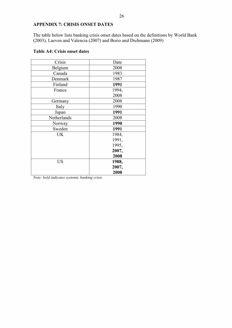
26

APPENDIX 7: CRISIS ONSET DATES

The table below lists banking crisis onset dates based on the definitions by World Bank

(2003), Laeven and Valencia (2007) and Borio and Drehmann (2009)

Table A4: Crisis onset dates

Crisis Date

Belgium 2008

Canada 1983

Denmark 1987

Finland 1991

France 1994,

2008

Germany 2008

Italy 1990

Japan 1991

Netherlands 2008

Norway 1990

Sweden 1991

UK 1984,

1991,

1995,

2007,

2008

US 1988,

2007,

2008 Note: bold indicates systemic banking crisis

27

APPENDIX 8: ADJUSTING THE OFF BALANCE SHEET PROXY TO REDUCE

CRISIS PROBABILITIES TO THE SAMPLE MEAN

We adjusted our proxy for OBS activity by the amount necessary to decrease the crisis

probability to our threshold value (0.055) in each country for every year in the sample. Table

A5 illustrates the results of the exercise, with zeros indicating that the probability of a crisis in

a country-year is already below 0.055 and no adjustment is necessary, while negative numbers

illustrating a required reduction in the change of OBS activity13

. Interpretation of the numbers

is not straightforward as we are looking at the second derivative rather than directly at the

movements in the ratios. But country by country and year by year comparisons still give us

useful insights into risk exposures and increased vulnerability.

Based on the table, different groups of countries are immediately identifiable; first, those

where none or almost no adjustment is required to OBS activity (Italy, Germany, Belgium);

second, those which had banking crises historically and showed an elevated level of OBS

exposures (Denmark, Finland, Sweden, Japan) and finally, countries where there was an

increase in OBS vulnerabilities in the run up to the subprime crisis (France, Spain, the UK

and the US). The last column of the table depicts the average adjustment for each year which

was necessary across all the countries. We have two periods where OBS activity was

excessive in relation to crisis risk, the largest adjustment was required for the period in the run

up to current financial meltdown and the second one was over the 1990’s when again many of

the countries in the sample experienced banking crises. On the other hand we should

emphasise that not all crises were related directly to OBS risk, as shown above – hence the

adjustment shown below is not always warranted by the current situation.

Table A5: Required adjustment in the change of off- to on-balance sheet activity in

order to keep crisis probability at in-sample mean level

BG CN DK FN FR GE IT JP NL NW SD SP UK US mean

1985 0.00 0.00 -0.53 -0.39 -0.30 0.00 0.00 -0.16 0.00 0.00 0.00 0.00 -0.18 0.00 -0.11

1986 0.00 0.00 0.00 -0.29 -0.03 0.00 0.00 -0.07 0.00 0.00 0.00 0.00 -0.49 0.00 -0.06

1987 0.00 -0.06 -1.32 -0.40 0.00 0.00 0.00 0.00 0.00 0.00 0.00 0.00 -0.23 0.00 -0.14

1988 0.00 -0.28 0.00 0.00 -0.12 0.00 0.00 0.00 0.00 -0.62 0.00 0.00 -0.38 -0.20 -0.11

1989 0.00 -0.48 0.00 0.00 -0.46 0.00 0.00 -0.08 0.00 -0.37 0.00 0.00 -1.01 -0.23 -0.19

1990 0.00 -0.57 0.00 -0.73 -0.52 0.00 0.00 -0.32 0.00 -1.21 0.00 0.00 -0.37 -0.11 -0.27

1991 0.00 -0.66 0.00 -0.99 -0.57 0.00 0.00 -0.07 0.00 0.00 -0.35 0.00 -1.90 -0.22 -0.341992 0.00 -0.25 0.00 -0.91 -0.54 0.00 0.00 -0.29 0.00 0.00 -0.40 0.00 -0.60 0.00 -0.21

1993 0.00 0.00 0.00 -0.30 -0.53 0.00 0.00 -0.08 0.00 0.00 -0.02 0.00 -0.05 0.00 -0.07

1994 0.00 0.00 0.00 -0.28 -0.43 0.00 0.00 0.00 0.00 0.00 -0.20 0.00 0.00 0.00 -0.07

1995 0.00 0.00 0.00 0.00 -0.41 0.00 0.00 0.00 0.00 0.00 0.00 0.00 0.00 0.00 -0.03

1996 0.00 0.00 0.00 0.00 0.00 0.00 0.00 0.00 0.00 0.00 0.00 0.00 0.00 0.00 0.00

1997 0.00 0.00 0.00 0.00 -0.26 0.00 0.00 -0.14 0.00 0.00 0.00 0.00 0.00 0.00 -0.031998 0.00 0.00 0.00 0.00 0.00 0.00 0.00 0.00 0.00 0.00 0.00 0.00 0.00 0.00 0.00

1999 0.00 -0.12 0.00 0.00 0.00 0.00 0.00 -1.07 0.00 0.00 0.00 0.00 0.00 0.00 -0.09

2000 0.00 0.00 -0.04 0.00 0.00 0.00 0.00 0.00 -0.04 0.00 -0.24 0.00 -0.25 0.00 -0.04

2001 0.00 0.00 0.00 0.00 0.00 0.00 0.00 0.00 -0.07 0.00 0.00 0.00 -0.52 -0.05 -0.05

2002 0.00 0.00 -0.20 0.00 -0.25 -0.06 0.00 0.00 -0.69 0.00 -0.05 0.00 -0.65 -0.06 -0.14

2003 0.00 0.00 0.00 0.00 -0.09 0.00 0.00 0.00 -0.51 0.00 -0.01 0.00 -0.63 -0.03 -0.09

2004 0.00 0.00 0.00 0.00 0.00 0.00 0.00 0.00 -0.04 0.00 0.00 0.00 -0.37 -0.14 -0.04

2005 0.00 0.00 0.00 0.00 0.00 0.00 0.00 0.00 0.00 0.00 0.00 -0.10 -0.77 0.00 -0.06

2006 0.00 0.00 -0.10 0.00 -0.43 0.00 0.00 0.00 0.00 0.00 0.00 -0.58 -1.19 0.00 -0.16

2007 0.00 0.00 0.00 0.00 -0.32 0.00 0.00 0.00 0.00 0.00 0.00 -1.10 -0.89 -0.07 -0.17

2008 -0.84 0.00 -0.77 0.00 -2.27 0.00 0.00 0.00 0.00 0.00 -0.55 -1.26 -0.80 -0.22 -0.48 Note: data in the table should be multiplied by 100, in order to be interpreted in percentage point terms

13

Years in the table refer to the date when probabilities are calculated, therefore as the d(off to on) variable is

lagged twice, the actual adjustment required to it is referred to the period two years prior (for example, the

probability for 1985 is calculated by taking into account d(off to on) in 1983, with the corresponding adjustment

is referring to 1983 as well).

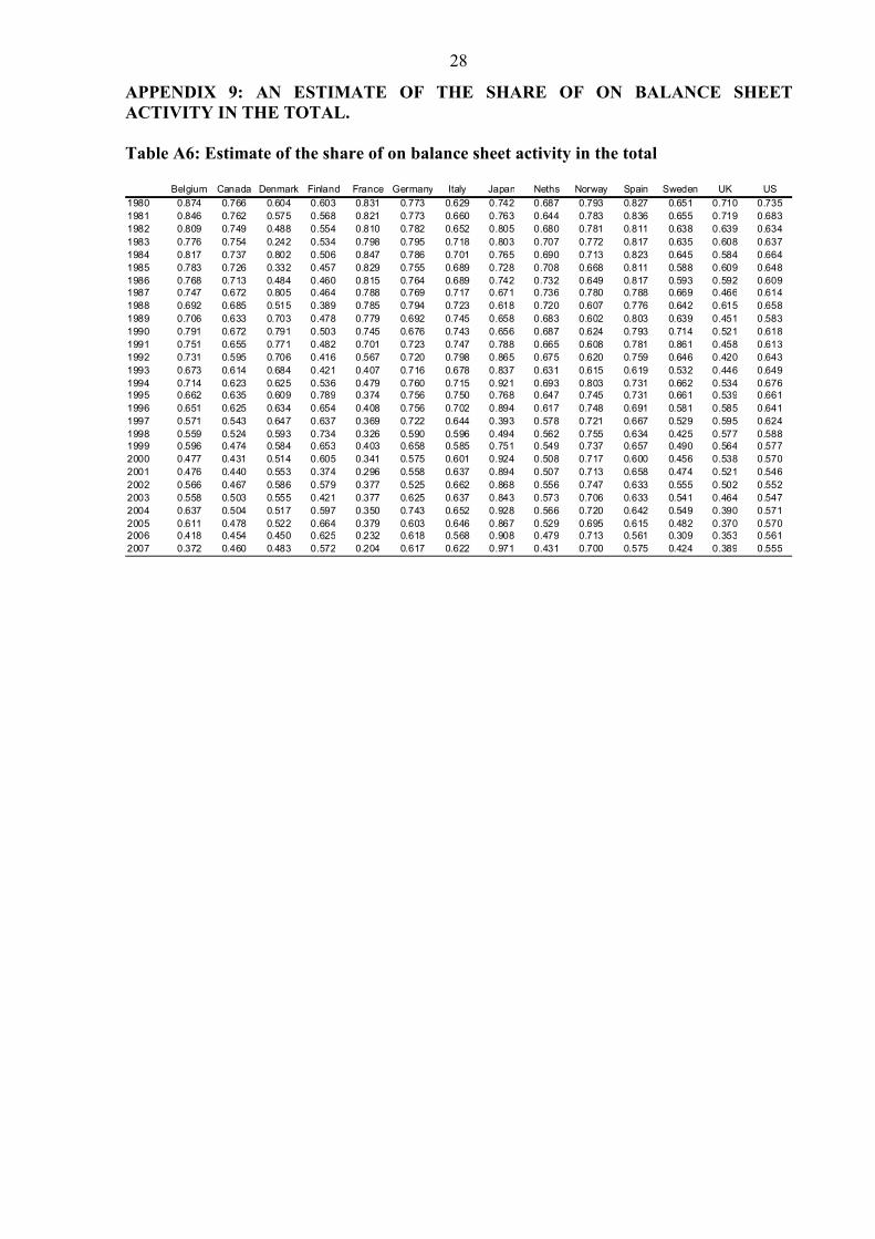
28

APPENDIX 9: AN ESTIMATE OF THE SHARE OF ON BALANCE SHEET

ACTIVITY IN THE TOTAL.

Table A6: Estimate of the share of on balance sheet activity in the total


1980 0.874 0.766 0.604 0.603 0.831 0.773 0.629 0.742 0.687 0.793 0.827 0.651 0.710 0.735

1981 0.846 0.762 0.575 0.568 0.821 0.773 0.660 0.763 0.644 0.783 0.836 0.655 0.719 0.683

1982 0.809 0.749 0.488 0.554 0.810 0.782 0.652 0.805 0.680 0.781 0.811 0.638 0.639 0.634

1983 0.776 0.754 0.242 0.534 0.798 0.795 0.718 0.803 0.707 0.772 0.817 0.635 0.608 0.637

1984 0.817 0.737 0.802 0.506 0.847 0.786 0.701 0.765 0.690 0.713 0.823 0.645 0.584 0.664

1985 0.783 0.726 0.332 0.457 0.829 0.755 0.689 0.728 0.708 0.668 0.811 0.588 0.609 0.648

1986 0.768 0.713 0.484 0.460 0.815 0.764 0.689 0.742 0.732 0.649 0.817 0.593 0.592 0.609

1987 0.747 0.672 0.805 0.464 0.788 0.769 0.717 0.671 0.736 0.780 0.788 0.669 0.466 0.614

1988 0.692 0.685 0.515 0.389 0.785 0.794 0.723 0.618 0.720 0.607 0.776 0.642 0.615 0.658

1989 0.706 0.633 0.703 0.478 0.779 0.692 0.745 0.658 0.683 0.602 0.803 0.639 0.451 0.583

1990 0.791 0.672 0.791 0.503 0.745 0.676 0.743 0.656 0.687 0.624 0.793 0.714 0.521 0.618

1991 0.751 0.655 0.771 0.482 0.701 0.723 0.747 0.788 0.665 0.608 0.781 0.861 0.458 0.613

1992 0.731 0.595 0.706 0.416 0.567 0.720 0.798 0.865 0.675 0.620 0.759 0.646 0.420 0.643

1993 0.673 0.614 0.684 0.421 0.407 0.716 0.678 0.837 0.631 0.615 0.619 0.532 0.446 0.649

1994 0.714 0.623 0.625 0.536 0.479 0.760 0.715 0.921 0.693 0.803 0.731 0.662 0.534 0.676

1995 0.662 0.635 0.609 0.789 0.374 0.756 0.750 0.768 0.647 0.745 0.731 0.661 0.539 0.661

1996 0.651 0.625 0.634 0.654 0.408 0.756 0.702 0.894 0.617 0.748 0.691 0.581 0.585 0.641

1997 0.571 0.543 0.647 0.637 0.369 0.722 0.644 0.393 0.578 0.721 0.667 0.529 0.595 0.624

1998 0.559 0.524 0.593 0.734 0.326 0.590 0.596 0.494 0.562 0.755 0.634 0.425 0.577 0.588

1999 0.596 0.474 0.584 0.653 0.403 0.658 0.585 0.751 0.549 0.737 0.657 0.490 0.564 0.577

2000 0.477 0.431 0.514 0.605 0.341 0.575 0.601 0.924 0.508 0.717 0.600 0.456 0.538 0.570

2001 0.476 0.440 0.553 0.374 0.296 0.558 0.637 0.894 0.507 0.713 0.658 0.474 0.521 0.546

2002 0.566 0.467 0.586 0.579 0.377 0.525 0.662 0.868 0.556 0.747 0.633 0.555 0.502 0.552

2003 0.558 0.503 0.555 0.421 0.377 0.625 0.637 0.843 0.573 0.706 0.633 0.541 0.464 0.547

2004 0.637 0.504 0.517 0.597 0.350 0.743 0.652 0.928 0.566 0.720 0.642 0.549 0.390 0.571

2005 0.611 0.478 0.522 0.664 0.379 0.603 0.646 0.867 0.529 0.695 0.615 0.482 0.370 0.570

2006 0.418 0.454 0.450 0.625 0.232 0.618 0.568 0.908 0.479 0.713 0.561 0.309 0.353 0.561

2007 0.372 0.460 0.483 0.572 0.204 0.617 0.622 0.971 0.431 0.700 0.575 0.424 0.389 0.555

evaluating off-balance sheet exposures in banking crisis ...

Documents

Transcript of evaluating off-balance sheet exposures in banking crisis ...