4/11/19

Evaluating dynamic treatment strategies

Barbra Dickerman Department of Epidemiology

Objectives • Define dynamic treatment strategies • Describe when g-methods are needed • Review an application of the parametric g-formula to

cancer research • Causal inference perspective

• Discuss the AI Clinician • Reinforcement learning perspective

Barbra Dickerman 2

1

●○○○

WHAT ARE DYNAMIC TREATMENT STRATEGIES?

Barbra Dickerman 3

Treatment strategies Point interventions Sustained strategies

Static Dynamic

1. Initiate treatment at baseline

2. Do not initiate treatment at baseline

1. Initiate treatment at baseline and continue over follow-up

2. Do not initiate treatment over follow-up

1. Initiate treatment at baseline and continue over follow-up, unless acontraindication occurs

2. Do not initiate treatment over follow-up, unlessan indication occurs

Barbra Dickerman 4

2

Dynamic treatment strategies • Take into consideration a patient’s evolving

characteristics before making a decision • Decisions about prevention, screening, or treatment

interventions over time may depend on evolving comorbidities,screening results, or treatment toxicity

• Strategies in clinical guidelines and practice are oftendynamic

• The optimal strategies will be dynamic

Barbra Dickerman 5

●●○○

WHEN ARE G-METHODS NEEDED?

Barbra Dickerman 6

3

Conventional statistical methods cannot appropriately comparedynamic strategies with treatment-confounder feedback

A

U

0 L1 A1 Y

At Vasopressors L1 Systolic blood pressure Y Survival U Disease severity

Barbra Dickerman 7

G-methods • Parametric g-formula • G-estimation of structural nested models • Inverse probability weighting of marginal structural

models

Barbra Dickerman 8

4

© Dickerman et al. All rights reserved. This content is excluded from our Creative Commons license. For more information, see https://ocw.mit.edu/help/faq-fair-use/

●●●○

CASE STUDY: PHYSICAL ACTIVITY AND SURVIVAL AMONG MEN WITH PROSTATE CANCER

Barbra Dickerman 9

Case study: Physical activity and survival among men with prostate cancer

Question • What is the effect of adhering to guideline-based

physical activity strategies on survival among menwith nonmetastatic prostate cancer?

Data • Health Professionals Follow-up Study (HPFS)

Barbra Dickerman 10

5

Physical activity and survival among men with prostate cancer

Eligibility criteria • Diagnosed with nonmetastatic prostate cancer at age 50-80 between1998-2010

• No cardiovascular/neurological condition limiting physical ability • Data on all potential confounders measured in the past 2 years

Initiate 1 of 6 physical activity strategies at diagnosis and continue it over Treatment strategies follow-up until the development of a condition limiting physical ability

Starts at diagnosis and ends at death, loss to follow-up, 10 years after Follow-up diagnosis, or administrative end of follow-up (June 2014), whicheverhappens first

All-cause mortality within 10 years of diagnosis Outcome Per-protocol effect Causal contrast Parametric g-formula Statistical analysis

Barbra Dickerman 11

Parametric g-formula • Generalization of standardization to time-varying exposures

and confounders • Conceptually, the g-formula risk is a weighted average of

risks conditional on a specified intervention history andobserved confounder history • The weights are the probability density functions of the time-varying

confounders, estimated using parametric regression models • The weighted average is approximated using Monte Carlo

simulation

Barbra Dickerman 12

6

Steps of the parametric g-formula

① Fit parametric regression models for treatment, confounders, and death at each follow-up time t as a function of treatment and covariate history among those under follow-up at time t

② Monte Carlo simulation to generate a 10,000-person populationunder each strategy by sampling with replacement from theoriginal study population (to estimate the standardized cumulativerisk under a given strategy)

③ Repeat in 500 bootstrap samples to obtain 95% confidence intervals (CIs)

Barbra Dickerman 13

Estimated risk of all-cause mortality underseveral physical activity strategies

All strategies excusemen from following therecommended physicalactivity levels afterdevelopment ofmetastasis, MI, stroke, CHF, ALS, or functional impairment

10-year Risk Strategy risk (%) 95% CI ratio 95% CI No intervention 15.4 (13.3, 17.7) 1.0 --Vigorous activity ≥1.25 h/week 13.0 (10.9, 15.4) 0.84 (0.75, 0.94) ≥2.5 h/week 11.1 (8.7, 14.1) 0.72 (0.58, 0.88) ≥3.75 h/week 10.5 (8.0, 13.5) 0.68 (0.53, 0.85) Moderate activity ≥2.5 h/week 13.9 (12.0, 16.0) 0.90 (0.84, 0.94) ≥5 h/week 12.6 (10.6, 14.7) 0.81 (0.73, 0.88) ≥7.5 h/week 12.2 (10.3, 14.4) 0.79 (0.71, 0.86)

Barbra Dickerman 14

7

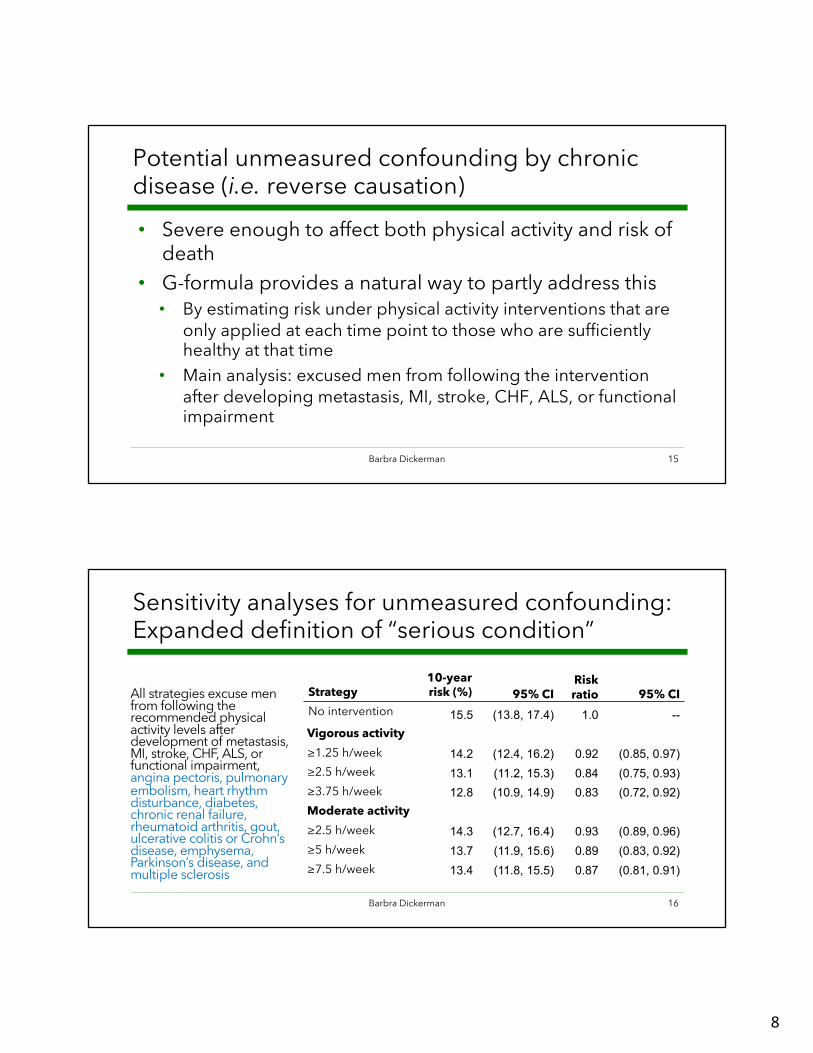
Potential unmeasured confounding by chronic disease (i.e. reverse causation) • Severe enough to affect both physical activity and risk of

death • G-formula provides a natural way to partly address this • By estimating risk under physical activity interventions that are

only applied at each time point to those who are sufficientlyhealthy at that time

• Main analysis: excused men from following the interventionafter developing metastasis, MI, stroke, CHF, ALS, or functionalimpairment

Barbra Dickerman 15

Sensitivity analyses for unmeasured confounding:Expanded definition of “serious condition”

All strategies excuse menfrom following therecommended physicalactivity levels afterdevelopment of metastasis,MI, stroke, CHF, ALS, orfunctional impairment, angina pectoris, pulmonary embolism, heart rhythmdisturbance, diabetes,chronic renal failure,rheumatoid arthritis, gout,ulcerative colitis or Crohn’sdisease, emphysema,Parkinson’s disease, andmultiple sclerosis

Strategy No intervention

Vigorous activity ≥1.25 h/week ≥2.5 h/week ≥3.75 h/week Moderate activity ≥2.5 h/week ≥5 h/week ≥7.5 h/week

10-yearrisk (%)

15.5

14.2 13.1 12.8

14.3 13.7 13.4

95% CI (13.8, 17.4)

(12.4, 16.2) (11.2, 15.3) (10.9, 14.9)

(12.7, 16.4) (11.9, 15.6) (11.8, 15.5)

Risk ratio

1.0

0.92 0.84 0.83

0.93 0.89 0.87

95% CI --

(0.85, 0.97) (0.75, 0.93) (0.72, 0.92)

(0.89, 0.96) (0.83, 0.92) (0.81, 0.91)

Barbra Dickerman 16

8

Sensitivity analyses for unmeasured confounding:Lag and negative outcome control • Lagged physical activity and covariate data by two years • Negative outcome control to detect potential unmeasured

confounding by clinical disease • Questionnaire non-response

Original analysis Negative outcome control

Barbra Dickerman 17

G-methods let us validly estimate the effect ofpre-specified dynamic strategies • And estimate adjusted absolute risks

• Appropriately adjusted survival curves • Not only hazard ratios • Even in the presence of treatment-confounder feedback

• Under the assumptions of exchangeability, consistency,positivity, no measurement error, no model misspecification

• Powerful approach to estimate the effects of currently recommended or proposed strategies

• But, these pre-specified strategies may not be the optimalstrategies

Barbra Dickerman 18

9

●●●●

© Springer Nature. All rights reserved. This content is excluded from our Creative Commons license. For more information, see https://ocw.mit.edu/help/faq-fair-use/

DISCUSSION: THE AI CLINICIAN

Barbra Dickerman 19

Barbra Dickerman 20

Komoroski et al. Nat Med 2018

Figure 1 Data flow of the AI Clinician

© Springer Nature. All rights reserved. This content is excluded from our Creative Commons license. For more information, see https://ocw.mit.edu/help/faq-fair-use/

10

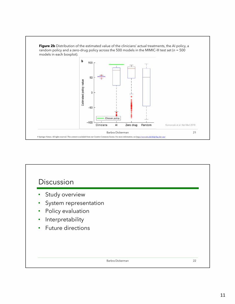
Figure 2b Distribution of the estimated value of the clinicians’ actual treatments, the AI policy, arandom policy and a zero-drug policy across the 500 models in the MIMIC-III test set (n = 500 models in each boxplot).

Komoroski et al. Nat Med 2018

Barbra Dickerman 21 © Springer Nature. All rights reserved. This content is excluded from our Creative Commons license. For more information, see https://ocw.mit.edu/help/faq-fair-use/

Discussion • Study overview • System representation • Policy evaluation • Interpretability • Future directions

Barbra Dickerman 22

11

MIT OpenCourseWare https://ocw.mit.edu

6.S897 / HST.956 Machine Learning for Healthcare Spring 2019

For information about citing these materials or our Terms of Use, visit: https://ocw.mit.edu/terms