European Asset Swap Spreads and the Credit Crisis · A further possible determinant of credit...

European Asset Swap Spreads and the Credit Crisis

Wolfgang Aussenegg(a)*, Lukas Götz(b), and Ranko Jelic(c)

(a) Department of Finance and Corporate Control, Vienna University of Technology

Address: Favoritenstrasse 9-11, A-1040 Vienna, Austria

E-mail: [email protected], Phone: +43 1 58801 33082 (b)

UNIQA Finanz-Service GmbH

Address: Untere Donaustraße 21, A-1029 Vienna, Austria

E-mail: [email protected], Phone: +43 1 211 75 2012 (c) Department of Accounting and Finance, University of Birmingham

Address: Birmingham, B15 2TT, United Kingdom

E-mail: [email protected], Phone: +44 (0) 121 414 5990

*Corresponding author

This Draft

May 2011 Acknowledgements: We would like to thank Alex Kostakis, Lawrence Kryzanowski, Jun Yang, as well as participants of the 2010 Financial Management Association European Meeting (Hamburg) for helpful comments and sug-gestions. We also thank Thomson Reuters for providing data.

1

Abstract The dynamics of credit risk are especially important for investors and bond issuing cor-

porations, e.g. for valuation or hedging purposes. In this study we focus on asset swap

(ASW) spreads as an increasingly important credit risk measure based on spot market

data. In particular we investigate the determinants of (ASW) spreads for a set of 23 Eu-

ropean corporate bond indices. Our results suggest that ASW spreads display significant

regime specific dynamics. During turbulent periods they are highly sensitive to equity

market volatility whilst in tranquil periods they exhibit a significant association with

stock returns. In contrast, the level of interest rates affects ASW spreads in both re-

gimes, whereas the difference between the swap curve and the government bond yield

curve (the swap spread) influences ASW spreads only in periods of increased volatility.

We also find evidence of negative autocorrelation of ASW spreads in tranquil and posi-

tive autocorrelation in turbulent periods.

JEL classification: C13, C32, G12

Keywords: European Bonds, Asset Swap Spreads, Credit Spreads, Financial Crisis,

Markov Switching

2

1. Introduction

By the end of 2008 the global credit derivatives market totaled approximately $39 tril-

lion.1 The largest part of the market consists of Credit Default Swaps (CDS). They are

essentially insurance contracts, where buyers agree to pay a predefined periodic fee (i.e.

CDS spread) while the sellers provide compensation in case of a default. Kakodkar et al.

(2003) demonstrate that CDS are comparable to asset-swapped fixed-rate bonds fi-

nanced in the repo market.2 In the strict sense asset swaps (ASW) are not credit deriva-

tives because they do not provide investors with protection against credit risk. However,

they are very closely associated with the credit derivatives market, because they sepa-

rate credit from interest rate risk.3

The ASW spread is a tradeable spread and, therefore,

the best cash market equivalent compared to CDS. Furthermore, they are usually traded

in a close range (see, e.g. Norden and Weber, 2009, or Zhu, 2004). For the above rea-

sons, the ASW spread is a widely accepted credit risk measure used by market partici-

pants.

More recently, CDS trading volumes dropped significantly to volumes that are now

bellow 30% of the record levels during pre-crisis levels.4 At the same time, the issuance

of corporate bonds and the liquidity of the ASW market increased to record levels in

2009. The increase is associated with increased holdings of both large and small retail

investors due to high returns in bond and ASW markets as well as losses on equity mar-

kets. According to IFSL Research (2009a; 2009b), during crisis periods, it was much

easier to participate in the ASW than the CDS market.5 The recorded changes in the

liquidity are consistent with evidence that ASW spreads tend to reveal information

about credit risk more efficiently than CDS spreads (Gomes, 2010).6

Furthermore, the

previous evidence report that ASW spreads measure credit risk more accurately than

bond spreads (De Wit, 2006; Felsenheimer, 2004; Fracis et al., 2003).

1 International Swaps and Derivatives Association’s (ISDA) Market Survey, 2009. 2 For example, by combining a fixed rate bond with a fixed-to-floating interest rate swap the bondholder effectively transforms the payoff, where she pays the fixed rate and receives the floating rate consisting of Libor plus the asset swap (ASW) spread. In case of a default the owner of the bond receives the recovery value and still has to honor the interest rate swap. Usual maturities are three and six months. 3 See, e.g. O’Kane and Sen (2004) for a thorough explanation of various forms of credit spreads. 4 See Boughey, S., Farewell to the CDS glory days, Financial News, 21 February 2011. 5 For example, the standard CDS notional amount is 2,000 times higher (for high-yield debt) then the standard corporate bond’s face value of €1,000. 6 This study examines a sample of 64 corporate bonds issued by 49 non-financial companies.

3

Whilst previous studies examine determinants of CDS index spreads (Byström, 2005;

Alexander and Kaeck, 2008), to the best of our knowledge, there are so far no other

studies that examine credit spreads based on ASW spreads derived from corporate bond

indices. The purpose of this study is to analyze the time-series dynamics of ASW

spreads for 23 European corporate bond indices. We extend the model of Alexander and

Kaeck (2008) by imposing a quality premium and by evaluating the time-varying beha-

vior of credit spreads. The examination of the time-varying behavior of credit spreads is

particularly important given the significant changes in nature of credit risk and the in-

creasing importance of the ASW market since 2008. This examination is also important

given recent regulatory changes introduced in the credit derivatives market.

We utilize an approach based on Markow switching models. Markov models provide an

intuitive and systematic way to model structural breaks and regime shifts in the data

generating process. Such models can be linear in each regime, but due to the stochastic

nature of the regime shifts nonlinear dynamics are incorporated. Another advantage of

this approach is the constantly updated estimate of the conditional state probability of

being in a particular state at a certain point in time. This approach conveys more precise

information about the switching process than a simple binary operator.

Our main findings are: (i) ASW spreads behave significantly different during periods of

financial turmoil compared to ‘normal’ periods, having a residual volatility which is up

to eight times higher compared to tranquil periods; (ii) structural determinants seem to

fit credit spreads better for financial sector companies than for the remaining industry

sectors; (iii) we find less evidence of regime switching in non - cyclical industry sec-

tors; (iv) especially, the financial sector shows a high degree of autocorrelation in credit

spreads, which is mostly negative in tranquil periods but highly positive in turbulent

market periods; (v) stock market volatility determines credit spreads mainly in turbulent

periods whereas stock returns are more important in periods of lower volatility; (vi)

interest rates are an important determinant in both market regimes; (vii) the quality

premium, defined as the difference between swap and government bond yield curve

tend to be relevant only in turbulent regimes; and (viii) positive returns in the stock

market and increases in interest rates tend to reduce the probability of entering the vola-

tile regime.

4

The remainder of this paper is organized as follows: Section 2 motivates our hypothes-

es. Section 3 describes the main characteristics of our sample. Results of OLS models

for determinants of European ASW spreads are provided in Section 4. In section five we

present results of our Markov switching models. Main drivers of the regime switching

are examined in section 6. Finally section 7 sums up and concludes.

2. Literature and hypotheses

The pricing of credit risk has evolved in two main approaches. First, reduced form

models treat default as an unpredictable event, where the time of default is specified as a

stochastic jump process.7 Second, structural models build on Merton (1974) and use

market and company fundamentals and allow the empirical testing of various determi-

nants of default.8

According to this approach, a default can only occur at maturity when

the firm value falls under a certain threshold.

Since structural models offer an economically intuitive framework to the pricing of cre-

dit risk, a large body of empirical literature has grown testing theoretical determinants

of credit spreads with market data.9

7 For a detailed description on several well known reduced-form models see, e.g. Jarrow, Lando, and Turnbull (1995), Duffie and Singleton (1999), or Hull and White (2000).

For example, the risk-free interest rate is expected

to be negatively related to default risk. Higher risk-free rates increase the risk-neutral

drift and lower the probability of default (Longstaff and Schwartz, 1995). Another ar-

gument supporting the inverse relationship between interest rates and credit spreads

refers to the business cycle. In periods of economic recessions interest rates tend to be

lower and corporate defaults tend to occur more often. In early empirical papers gov-

ernment bond yields were used as a proxy for the risk-free rate. Although swap interest

rates are not completely free of risk, as they reflect the interbank market risk, they are

often regarded as a better benchmark for the risk-free rate than government yields

8 Several extensions of Merton’s original model have been formulated. In the model of Black and Cox (1976) default can take place at any time. Leland (1994) relates debt value and capital structure to the leverage a company is assuming. Longstaff and Schwartz (1995) allow a more complex liability structure and introduce stochastic interest rates in their model. Zhou (2001) specifies the movement of the firm value as a jump-diffusion process. Hui and Lo (2002) introduce macro-economic variables and model the default threshold as a stochastic process. 9 See, e.g. Huang and Kong (2003); King and Khang (2002); Duffee (1998); Collin-Dufresne et al. (2001); Elton et al. (2001); Longstaff et al. (2005).

5

(Houweling and Vorst, 2005). For example, they do not suffer from temporary pikes

sometimes caused by characteristics of repo agreements involving government bonds.

Furthermore, swaps have no short sale constraint, are less influenced by regulatory or

taxation issues, and tend not to be affected by scarcity premiums in times of shrinking

budget austerity. Finally, swap rates closely correspond to the funding costs of market

participants (see, e.g. Houweling and Vorst, 2005; or Hull et al., 2004). This leads to

our first hypothesis:

Hypothesis 1: ASW spreads based on European iBoxx bond indices are negatively asso-

ciated with the level of interest rates, measured by swap interest rates.

Another key variable in the structural framework is the leverage ratio, defined as the

ratio of a firm’s debt to its firm value. When the ratio approaches unity default is trig-

gered, thus a lower firm value (and therefore also a lower equity value) increases the

probability of default. Similarly, an increase in volatility increases the probability of

default, and, therefore, also increases the credit spread. Firm value and firm value vola-

tility are typically not directly observable. As proxies for these two variables we are

using the implied volatility of traded options and stock market returns (a higher stock

market valuation implies higher firm values and, therefore, a lower probability of de-

fault). This leads to two further hypotheses:

Hypothesis 2: ASW spreads based on European iBoxx corporate bond indices are nega-

tively associated with stock market returns.

Hypothesis 3: ASW spreads based on European iBoxx corporate bond indices are posi-

tively associated with stock market volatility.

A further possible determinant of credit spreads is the swap spread, which is defined as

the difference between the swap interest rate and the interest rate of a par value Trea-

sury bond of the same maturity. This difference is normally associated with liquidity

and default risk (see, e.g. Duffie and Singleton, 1999). More recently, Feldhütter and

Lando (2008) decompose the swap spread into a credit risk element, a convenience

premium and idiosyncratic risk factors. They conclude that the major determinant of

swap spreads is the convenience yield defined as investors’ willingness to pay a pre-

6

mium for the liquidity of Government bonds (see also Grinblatt, 2001). Longstaff

(2004) shows that this effect (labeled flight to quality) is especially apparent when mar-

kets are unsettled. This has direct consequences for the swap spread. A change in the

market’s perception of risk is reflected in a widening spread and occurs when investors

become concerned about liquidity in financial markets. They redirect their funds to the

highest credit quality and most liquid securities – government bonds. Due to the high

demand, government bond yields usually fall in such an environment more than those of

other credit securities, which further leads to an increase in the swap spread. For the

above reasons, Liu et al. (2006) recommend the swap spread as an ideal indicator of

default and liquidity risks associated with returns of fixed income securities.10

Empirical evidence for the association of swap spreads and credit spreads is provided

for several markets. For example, Brown et al. (2002) report a significant positive rela-

tionship between swap and credit spreads in the Australian market. Kobor et al. (2005)

find a positive long-term relationship between swap spreads and credit spreads for U.S.

AA-rated bonds with maturities of two, five and ten years. And finally, Schlecker

(2009) documents a cointegration relationship of credit spreads with swap spreads for

the U.S. as well as the European corporate bond market. This leads to our fourth hypo-

thesis:

Hypothesis 4: ASW spreads based on European iBoxx corporate bond indices are posi-

tively associated with swap spreads.

3. Data and sample characteristics

Our sample consists of Asset Swap (ASW) spreads for 23 different European iBoxx

Corporate Bond indices.11

10 Another commonly used barometer of the market’s perception of risk is the Euribor-OIS spread. It reflects investor’s perception of the default risk of banks. The spread of the Euribor and the overnight indexed swap (OIS) becomes wider if banks are reluctant to lend money to each other due to higher risk in financial markets. For the empirical part of this study, however, we resort to the swap spread as deter-minant for ASW spreads, because the Euribor-OIS spread is too noisy for our daily data sample.

In our analysis we focus on the period from January, 1st 2006

until January, 30th 2009, including 779 trading days. Sample bond indices are grouped

11 iBoxx is a leading fixed income index provider serving to establish benchmarks for asset managers and investors.

7

based on the classification and criteria provided by Markit.12 For example, the market

capitalization weighted iBoxx Benchmark indices consist of liquid bonds with a mini-

mum amount outstanding of at least €500 million and a minimum time to maturity of

one year. Furthermore, the bonds need to have an investment grade rating and a fixed

coupon rate. The indices are rebalanced monthly. The bond index values are calculated

daily based on market prices, thus they represent the most accurate and timely bond

pricing available. The ASW spreads provided by Markit are derived from prices of the

underlying bonds included in the respective iBoxx index and ICAP swap rates.13

Time

series of swap and government bond yield curves are from Datastream.

Descriptive statistics for the sample of ASW spreads are provided in Table 1. The indic-

es are stratified as non-financial industrial sectors (Automobiles & Parts, Chemicals,

Food & Beverage, Health Care, Oil & Gas, Personal & Household Goods, Retail, Tele-

communications, and Utility), financials (Senior, Subordinated, Banks, Tier 1 Capital,

and Lower Tier 2 Capital), credit rating (AAA, AA, A, and BBB), and seniority (Senior

and Subordinated). Corporate Composite is a composite index and includes 1,082 cor-

porate bonds that constitute all sample indices. The average size of our bonds included

in the Corporate Composite index amounts to €910.4 million. AAA-rated bonds have

the highest volume with an average issue size of more than €1.3 billion. The notional

amount of all bonds in our sample totals €985 billion by the end of January 2009.

The average time to maturity of all bonds included in the Corporate Composite index is

5.28 years. Given that the most liquid CDS spreads have 5-year maturity we can com-

pare our results directly to the results reported in previous studies based on CDS spreads

(see, e.g. Alexander and Kaeck, 2008). The median daily change is highest for Tier 1

Capital ASW spreads and lowest for Health Care and Telecommunication sectors. The

values for the annualized standard deviation highlight significant time series variation.

For the Tier 1 Capital industry sample the annualized standard deviation amounts to

100.9 basis points (bps) per year, whereas ASW spreads in the Utility sector only exhi-

bit a value of 42.6 bps. Turning to higher moments, daily spread changes are highly

leptokurtic for all sectors. The skewness of spreads is generally positive, with extreme

12 Markit sorts all bonds into industry classes based on ICB (Industry Classification Benchmark). 13 ICAP is the world largest broker house with a daily transaction volume in range of $1.5 billion.

8

values for Banks, Tier 1 Capital and AAA-rated corporate bonds. These three sectors

exhibit the highest level of skewness and excess-kurtosis in our sample.

*** Insert Table 1 about here ***

The mean spread for the Corporate Composite Index is 87.8 basis points. It is worth

mentioning that the Corporates AAA index only contains one non-financial bond (is-

sued by health care company Johnson & Johnson). The remaining 35 bonds in this sec-

tor represent debt raised by highly rated financial institutions.

Across industries, our ASW spread sample clearly shows higher diversity since early

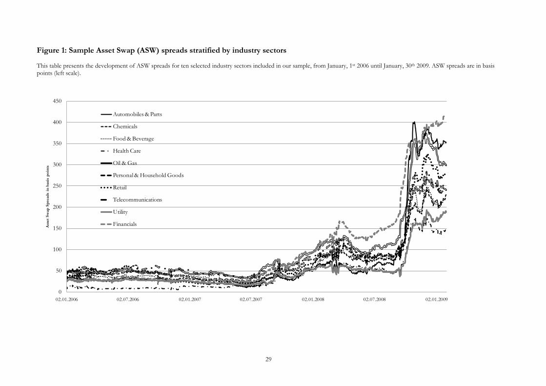
2008. Figure 1 tracks the co-movement of ASW spreads for ten different industry sec-

tors. As expected, the ASW spreads for the financial sector dominate spreads for all

other industries. Other sectors with above-average spreads during the credit crises (es-

pecially in the year 2008) are Oil & Gas as well as Automobiles & Parts.

*** Insert Figure 1 about here ***

4. Determinants of Asset Swap spreads

We start our analysis with the following linear regression model to determine changes

in ASW spreads:

ΔASW𝑘,𝑡 = 𝛽𝑘,0 + 𝛽𝑘,1ΔASW𝑘,𝑡−1 + 𝛽𝑘,2Stock return𝑘,𝑡 + 𝛽𝑘,3ΔVStoxx𝑡 + 𝛽𝑘,4ΔIR− Level𝑡 + 𝛽𝑘,5ΔSwap Spread𝑡 + 𝜀𝑘,𝑡 (1)

where ΔASW𝑘,𝑡 is the change in the ASW spread of industry sector k on day 𝑡,

ΔASW𝑘,𝑡−1 is the one period lagged ASW spread return, Stock return𝑘,𝑡 represents daily

returns of the stock index for sector k, ΔVStoxx𝑡 is the change in the VStoxx volatility

index, ΔIR − Level𝑡 denotes the change in the level of the interest rate swap curve

9

(based on the first principal component)14

, and ΔSwap Spread𝑡 represents swap spread

changes.

Equity values are proxied by the DJ Euro Stoxx indices which are also provided by

Markit and exist for almost all sectors analyzed in this study (ΔStock return𝑘,𝑡). The

equity value proxy for non-financials is the FTSE World Europe ex Financials stock

index, as Markit does not offer such an index (see also Table 1). We choose the VStoxx

index (ΔVStoxx𝑡) as a proxy for the implied volatility, since it is the reference measure

for the volatility in European markets. The final determinant included in model (1) is

the swap spread (ΔSwap Spread𝑡), measured as the difference between the five year

European interest rate swap rate and the yield of German government bonds of the same

maturity. Due to empirical evidence we consider the swap spread as a quality premium,

as it mainly comprises default risk and a convenience premium for holding risk-less

Treasury bonds.15

Byström (2006) examines determinants of CDS iTraxx index spreads and includes

lagged spread changes in his model. He reports a high degree of autocorrelation in daily

changes for all industry sectors. Byström (2006) concludes that it is not possible to ex-

ploit this inefficiency, after controlling for transaction costs. Since ASW spreads

represent the cash-market equivalent to CDS spreads, a similar pattern is expected. Un-

reported results suggest that 15 of the 23 sample ASW spreads exhibit a highly signifi-

cant degree of autocorrelation with mixed signs. Thus, the inclusion of lagged spread

changes (ΔASW𝑘,𝑡−1) as a control variable is motivated by empirical observations in

previous studies.

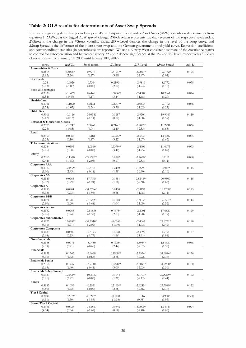
The results of the regressions are presented in Table 2. They reveal that the sign of the

coefficients are mostly consistent with our predictions. All but one sector exhibit a neg-

ative relationship between ASW spreads and the level of interest rates (ΔIR − Level𝑡).

This observation supports hypothesis 1. In addition, the stock market variables influence

ASW spreads of most industry sectors negatively, implying higher spreads when stock

markets decrease. This observation is consistent with hypothesis 2, although a signifi-

14 European interest rate swap rates with maturities between one and ten years are used to calculate the first principal component. 15 See, for example, Brown et al. (2002), Kobor et al. (2005), or Schlecker (2009).

10

cant negative association only can be observed for three sectors (Utilities, A-rated Cor-

porate, and Corporate Subordinated). Consistent with hypothesis 3, the results document

a positive association between stock market volatility and ASW spreads in 21 of 23 cas-

es.16

Overall, volatility seems to have a larger impact on ASW spreads than equity re-

turns.


Turning to the swap spread, ASW spread changes of all 23 groups are positively asso-

ciated with swap spread changes (ΔSwap Spreadt). This observation is in line with hy-

pothesis 4. Furthermore, lagged changes of ASW spreads are only in five cases signifi-

cant positive (at the 5% level), whereas six groups exhibit a negative but not significant

autocorrelation (see ΔASW𝑡−1 in Table 2). The explanatory power of the models is

clearly higher for the financial sector than for non-financial sectors - with the exception

of the Automobiles & Parts sector. By far the best explained sector is Tier 1 Capital

with an adjusted R2 of 35%.

Cossin et al. (2002) find for the US market, that changes in structural variables affect

companies with a high rating less than low rated companies. Our results in subsamples

with different credit ratings are mixed. Although Subordinated Corporates are better

explained than Senior Corporates the opposite is true for AAA-rated companies com-

pared to BBB-rated firms. Furthermore, Financials Senior and Subordinated spreads are

nearly equally well explained.

5. Structural breaks and regime switching

5.1 Structural breaks

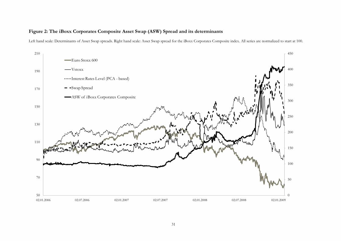
The evolution of ASW spreads of the iBoxx Corporate Bond indices and its determi-

nants during the credit crisis is illustrated in Figure 2. The stock market increased stea-

16 12 of the 21 cases are significant, and the two cases with negative coefficients are not significant at the 5% level.

11

dily until summer of 2007 and lost more than half of its value in the following 18

months. The level of interest rates peaked in the summer of 2008 and sharply declined

until the end of our sample period. Conversely, implied volatility, measured by the

VStoxx index, the swap spread, specified as the difference between the swap curve and

German government bond yields, as well as ASW spreads of the Corporate Composite

bond index are relatively tranquil until the middle of 2007. They increase sharply for the

following 14 months and jump in September 2008 to remain at a high level until the

beginning of January 2009.


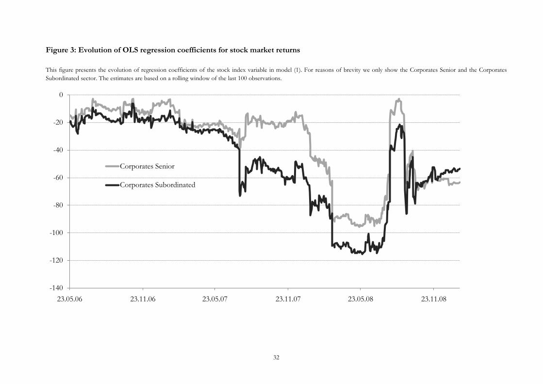
Figure 3 depicts the evolution of regression coefficients of the stock index variable in

model (1). For reasons of brevity we only show the Corporates Senior index and the

Corporates Subordinated sector. The influence of the stock market seems to be only

slightly increasing until the summer of 2007, when there is reason to expect a structural

break. From mid 2007 to the very end of our sample period the stock market has a high-

ly time-varying influence on ASW spreads with regression coefficients ranging from -3

to -96 (Corporates Senior) and -54 to -115 (Corporates Subordinated), respectively. The

results for all other indices exhibit a very similar pattern.


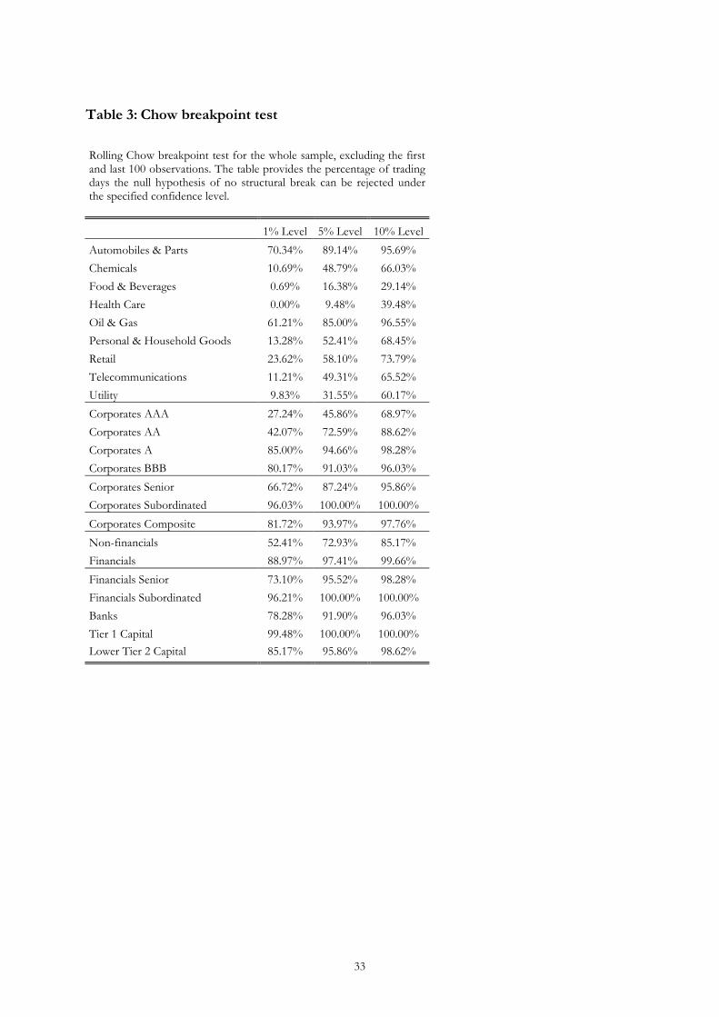
To statistically quantify potential structural breaks in the time-series of the data we em-

ploy a Chow breakpoint test for all dates in the sample apart from the first and last 100

observations. The null hypothesis of no structural break in the data is rejected at the 1%

level of significance for 81.72% of daily observations (see Table 4: Corporate Compo-

site sample). Results for most other sectors are similar. Extreme values are observable

for the Tier 1 Capital index where in 99.48% of all observations the null hypothesis of

no structural breaks can be rejected at the 1% significance level. On the other hand, for

Food & Beverage, Utility, and Health Care sectors the null hypothesis is rejected (at the

1% significance level) for less than 10% of observations.

12


5.2 Markov switching model

The previously reported results suggest the time-varying properties of the parameters

and the leptokurtosis of our sample. It is, therefore, important to estimate a nonlinear

model where different regimes can be defined allowing for dynamic shifts of economic

variables at any given point in time conditional on an unobservable state variable 𝑠𝑡.

Markov switching models provide an intuitive and systematic way to model structural

breaks and regime shifts in the data generating process.17

Such models can be linear in

each regime, but due to the stochastic nature of the regime shifts nonlinear dynamics are

incorporated. Furthermore, the specification consists of a mixture of distributions which

generates the leptokurtosis, as the variances in the two regimes differ. Another advan-

tage of using a latent variable 𝑠𝑡 is the constantly updated estimate of the conditional

state probability of being in a particular state at a certain point in time. This approach

conveys more precise information about the switching process than a simple binary op-

erator.

We estimate a two-state Markov model to explain ASW spread changes (ΔASW𝑘,𝑡) for

each sector 𝑘:18

ΔASWk,t = 𝛽𝑆,𝑘,0 + 𝛽𝑆,𝑘,1ΔASWk,t−1 + 𝛽𝑆,𝑘,2Stock return𝑘,𝑡 + 𝛽𝑆,𝑘,3ΔVStoxxt

+ 𝛽𝑆,𝑘,4ΔIR− Level𝑡 + 𝛽𝑆,𝑘,5ΔSwap Spread𝑡 + 𝜀𝑆,𝑘,𝑡 (2)

where 𝛽𝑆,𝑘,𝑗 is a matrix of 𝑗 regression coefficients as used in model (1) of the kth sector,

which are dependent on the state parameter 𝑠. The explanatory variables are ΔASW𝑘,𝑡−1,

which is the one period lagged ASW spread change, Stock return𝑘,𝑡 represents the dai-

ly returns of the stock index for sector k, ΔVStoxxt is the change in the VStoxx volatili-

ty index, ΔIR − Level𝑡 denotes the change in the level of the interest rate swap curve 17 For various applications of Markov switching models related to interest rates, bond markets, and credit risk modeling, see, e.g. Clarida (2006), Brooks and Persand (2001), Eyigunor (2006), or Dionne et al. (2007). 18 The formulation used in our analysis is adopted from Hamilton (1989) who uses an iterative algorithm, similar in spirit to a Kalman filter.

13

based on the first principal component, and ΔSwap Spread𝑡 represents swap spread

changes. Finally, 𝜀𝑆,𝑘,𝑡 is a vector of disturbance terms, assumed to be normal with

state-dependent variance 𝜎𝑆,𝑘,𝑡2 .

In our specification the state parameter 𝑠𝑡 is assumed to follow a first-order, two-state

Markov chain where the transition probabilities are assumed to be constant:19

𝑃𝑟𝑜𝑏 {𝑠𝑡 = 𝑗|𝑠𝑡−1 = 𝑖, 𝑠𝑡−2 = ℎ, … } = 𝑃𝑟𝑜𝑏 {𝑠𝑡 = 𝑗|𝑠𝑡−1 = 𝑖} = 𝑝𝑖𝑗 (3)

and can be summarized in matrix 𝑃: 20

𝑃 = �𝑝11 𝑝12𝑝21 𝑝22� = � 𝑝11 1 − 𝑝22

1 − 𝑝11 𝑝22� = 𝑝𝑖𝑗 (4)

Due to the fact that we cannot observe 𝑠𝑡 directly, we can only make an inference about

the state of the regime at time 𝑡 and have to assign probabilities of being in one regime.

If we let the vector 𝜉𝑡 represent a Markov chain with 𝜉𝑡 = (1, 0)′ when 𝑠𝑡 = 1 and

𝜉𝑡 = (0, 1)′ when 𝑠𝑡 = 2, the conditional expectation of 𝜉𝑡+1 given 𝑠𝑡 = 𝑖 is

𝔼(𝜉𝑡+1|𝑠𝑡 = 𝑖) = �𝑝𝑖1𝑝𝑖2

� = 𝑃 𝜉𝑡 (5)

Assuming Gaussian residuals 𝜀𝑆,𝑘,𝑡 for both states 𝑖, the conditional densities of 𝑓(𝑦𝑡)

are collected in a 2 × 1 vector 𝜂𝑖,𝑡 whose elements are given by21

𝜂𝑖,𝑡 = 𝑓(𝑦𝑡|𝑠𝑡 = 𝑖, Ω𝑡−1,𝜃) = 1𝜎𝑖√2𝜋

𝑒−�𝑦𝑡−𝑥𝑡

′ 𝛽𝑖�2

2𝜎𝑖2 , (6)

19 Adapted from Hamilton (1989) and Alexander and Kaeck (2008). 20 Our specification consists of two states that (as we can see later) can be interpreted as volatile and tran-quil market regime. 21 See, e.g. Hamilton (1989) or Alexander and Kaeck (2008).

14

where 𝜃 is a vector of state-dependent population parameters, which in our model is

𝜃 = (P, βi, σi). Ω𝑡−1 denotes the information up to time 𝑡 − 1. To obtain the conditional

state probabilities one has to solve recursively the pair of equations (7) and (8):

𝜉𝑡|𝑡 = 𝜉�𝑡|𝑡−1 ⨀ 𝜂𝑡

1′(𝜉�𝑡|𝑡−1 ⨀ 𝜂𝑡) (7)

𝜉𝑡+1|𝑡 = 𝑃𝜉𝑡|𝑡, (8)

where 𝜉𝑡|𝑡 represents the filtered probability for each state estimated at time 𝑡, given all

information up to time 𝑡 and ⨀ denotes element-by-element multiplication. The nume-

rator in equation (7) represents the density of the observed vector 𝑦𝑡 conditional on all

past observations. The 𝑡𝑡ℎ element of the product 𝜉𝑡|𝑡−1 ⨀ 𝜂𝑡 can be interpreted as the

conditional joint density distribution of 𝑦𝑡 and 𝑠𝑡 = 𝑖.

Iterating through equations (7) and (8) leads to the sample conditional log likelihood:22

𝐿(𝜃) = ∑ 𝑙𝑛𝑇𝑡=1 𝑓(𝑦𝑡|Ω𝑡−1;𝜃) = ∑ 𝑙𝑛𝑇

𝑡=1 (1′(𝜉𝑡|𝑡−1 ⨀ 𝜂𝑡)), (9)

where the set of optimal parameter values 𝜃 can be calculated numerically by maximiz-

ing the log likelihood function under the constraints that 0 < 𝑝𝑖𝑖 < 1 and 𝜎𝑖 ≥ 0.

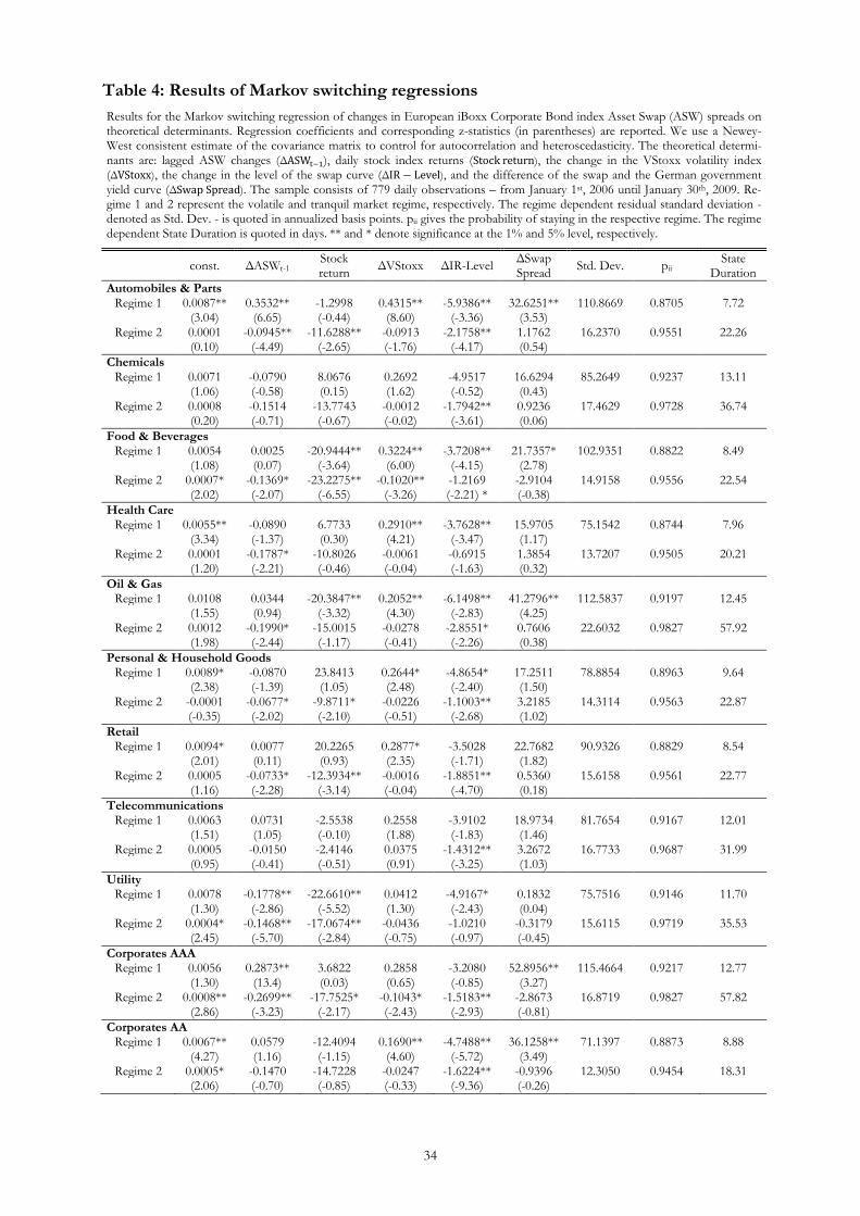
5.3 Results of the Markov switching model

We proceed by estimating model (2) with the above mentioned specification. Results of

the Markov switching regression are provided in Table 4.23


22 See, e.g. Hamilton (1989) or Alexander and Kaeck (2008). 23 Matlab R2009b was used for computing the Markov Switching regressions.

15

The output of the Markov switching model indicates that the estimated coefficients dif-

fer considerably between the two market regimes. The residual volatility (Std. Dev.) is

between four and eight times higher during turbulent than in tranquil market periods.

Perhaps the most striking result is the significantly different structure of the autocorrela-

tion coefficient (ΔASW𝑡−1) in the two regimes. The majority of all sectors under inves-

tigation exhibit a negative autocorrelation during the low volatility regime (Regime 2)

and positive autocorrelation in times of high volatility (Regime 1), indicating that the

data generating process consists of a mixture of different distributions. This phenome-

non also explains why most of the lagged credit spread changes (ΔASW𝑡−1) have not

been significant in the OLS model. The positive autocorrelation effect in the volatile

regime is most pronounced for the sectors Automobile & Parts, AAA-rated Corporates,

as well as most financial sectors.

Stock market returns have a significant negative effect on credit spreads in the second

(tranquil) regime. This is especially true for financial sector firms and within this group

for subordinated financials, banks, Tier 1 Capital, and Lower Tier 2 Capital. For these

sectors increasing stock prices in low volatile periods are associated with lower ASW

spreads. Again, non-financial firms behave differently. For them stock market returns

are not significantly related to ASW spread changes, neither in the high nor in the low

volatile regime.

Opposite to stock market returns, changes in the VStoxx influence ASW spreads espe-

cially in the high volatility regime (Regime 1). For all but one of the 23 sectors the rela-

tionship is positive (in 10 out of the 22 sectors significant at the 5% level). On the other

hand, in the low volatility regime (Regime 2) the relationship is predominantly nega-

tive. Thus, an increasing volatility in the stock market increases ASW spreads in a vola-

tile regime but tend to decrease ASW spreads in tranquil periods. This result is in line

with Alexander and Kaeck (2008), who report similar results for changes in CDS spread

indices.

The interest rate level (ΔIR − Level𝑡) affects ASW spreads negatively in both regimes

(in 45 out of 46 cases, 31 of the 45 cases are significant at the 5% level). This implies

that an increase in interest rates is regime independent associated with a drop in spreads,

which is in line with hypotheses 1, but is in contrast to Alexander and Kaeck (2008)

16

focusing on CDS spreads. Table 4 also reveals that the negative coefficient in the vola-

tile regime (Regime 1) is always larger in absolute terms compared to the negative coef-

ficient in the tranquil regime (Regime 2). This indicates that decreasing interest rates in

stormy periods tend to increase spreads more than in more quiet periods.

Finally, the influence of the swap spread (ΔSwap Spread𝑡) is always positive during

periods of stress in financial markets (Regime 1).24

This evidence is in line with the

prediction formulated in hypothesis 4. The swap spread, which serves as a quality pre-

mium, is an optimal proxy for the perceived liquidity risk in the market. It is highly sig-

nificant in periods of turmoil but does not explain spreads in tranquil times. Although

19 out of 23 sectors exhibit also a positive coefficient in Regime 2 (low volatility pe-

riod) these coefficients are not significant at the 5% level.

In order to evaluate the effectiveness of the Markov switching model compared to clas-

sical non-switching regressions we test if there is any switching in the parameters. Un-

fortunately formal standard statistical tests of OLS models against a regime switching

model are not valid due to unidentified parameters under the null hypothesis, thus they

do not converge to their assumed distribution and asymptotic theory cannot be applied.

An alternative is proposed by Engel and Hamilton (1990). They suggest a classical log

likelihood ratio test with the null hypothesis (𝐻0) of no switching in the coefficients

(𝛽𝑆𝑡=1 and 𝛽𝑆𝑡=2) but allow for switching in the residual variance (𝜎𝑆𝑡=1 and 𝜎𝑆𝑡=2).

Thus we test the following hypothesis:

𝐻0 ∶ 𝛽𝑆𝑡=1,𝑗 = 𝛽𝑆𝑡=2,𝑗 for all 𝑗, 𝜎𝑆𝑡=1 ≠ 𝜎𝑆𝑡=2 (10)

This specification is clearly more conservative than the hypothesis that both are switch-

ing. The likelihood ratio is asymptotically 𝜒(5)2 distributed. The corresponding results

are reported in Table 5.


24 The coefficients of all 23 cases are positive, 16 of them are significant at the 5% level.

17

For all 23 sectors the null hypothesis of equal coefficients in both regimes can be re-

jected at the 5% level. Generally Financials provide most evidence of regimes switching

with the Tier 1 Capital sector having the highest LR-statistic.

Regime specific moments of ASW spreads are compared in Table 6. The standard devi-

ations of the residuals in the tranquil regime are significantly lower than the residuals in

the first regime (high volatility regime). Spread changes in regime 2 (tranquil) are closer

to normality with an average change of 0.10 basis points (Corporate Composite), an

average skewness of 0.44 and an average excess kurtosis of 0.64. Contrary, the spread

changes in the turbulent regime are much more non-normal. Daily spread changes have

an average of 1.19 basis points, a skewness of 0.87 and an excess kurtosis of 2.29. Not-

able, the distribution of spread changes of AAA-rated Corporates and Banks is highly

leptokurtic with an excess kurtosis of 6.75 and 13.2, respectively, whereas the excess

kurtosis is lowest for the Retail sector.


The first column of Table 6 presents the amount of time (in percentage terms) a volatile

regime is predominant. The mean value for all sectors, excluding financials, is 26.8%,

whereas it is 39.3% for finance-related sectors. This result may not come as a surprise,

given that our sample includes the credit crisis during which financial companies have

lost a significant part of their market value.

6. Determinants of regime changes

Having identified two distinct regimes, a high volatility regime and a relatively tranquil

regime with low volatility, we investigate which explanatory indicators drive the regime

transition. At first, Figure 4 presents the relationship between the regime probabilities

and the ASW spread volatility. The figure depicts a positive association between the

probabilities and ASW spread volatility.

18


The US housing bubble came to a sudden end when housing prices started to flatten and

eventually dropped by a median of 3.3% in the first quarter of 2006 compared to the last

quarter of 2005. Consequently the first three months of our sample are dominated by a

phase of high volatility in financial markets (see event 1 in Figure 4). The scale of the

financial crisis was heralded as Ameriquest Mortgage, once one of the largest subprime

lenders, revealed plans in May 2006 to close its retail branches and announced signifi-

cant job cuts (see event 2 in Figure 4). We did not enter the volatile state again until

November 2006 when financial markets rallied to a five year high leading to an ASW

spread reduction of 7 basis points.

Another volatile period started when credit markets froze in summer 2007 (see event 3

in Figure 4). Lenders stopped offering home equity loans. In a coordinated move the

Federal Reserve and the European Central Bank injected $100 billion and €95 billion,

respectively, into the banking system. Countrywide, America’s largest mortgage lender

had to take out an emergency loan to avoid bankruptcy. At the end of August 2007

Ameriquest Mortgage finally went out of business and on September 4th, 2007, Libor

rates rose to 6.79%, the highest level since 1998. During the following four months

ASW spreads returned to the tranquil regime lasting until the January 2008 stock market

downturn, which eventually lead to the emergency sale of Bear Stearns (at that time the

fifth largest investment bank in the world), to rival JP Morgan on March 16th, 2008 (see

event 4 in Figure 4). Within the first 11 trading days in March 2008, the Corporate

Composite ASW spread jumped by more than 33 basis points, with a maximum daily

change of 19.15 basis points. For the following five months of our sample we only enter

the volatile regime occasionally. During this period Indymac Bank, the seventh-largest

mortgage originator was placed into receivership of the FDIC by the Office of Thrift

Supervision.

Starting in late August of 2008 we basically remain in the volatile regime until the end

of our sample. Freddie Mac and Fannie Mae guaranteeing a combined $12 trillion were

nationalized at the beginning of September 2008 (see event 5 in Figure 4). Rumors

about liquidity problems of investment bank Lehman Brothers surfaced. Eventually the

19

company filed for bankruptcy protection on September 15th, 2008 marking the peak of

the financial crisis (see event 6 in Figure 4). Within 23 trading days the Corporate

Composite ASW spread exploded by 144 basis points with a single day jump of 17.4

points on September 16th, 2008. Days later it became public that AIG was on the brink

of bankruptcy, causing the ASW spread to increase nearly 16 basis points within a day

and the Federal Reserve lending $85 billion to the troubled company.

The last and largest spike in Asset Swap spreads in our sample occurred on November

21st, 2008 when the value of the Corporate Composite ASW spread jumped by 20.06

basis points caused by liquidity problems of Citigroup (see event 7 in Figure 4). The

stock value of the once biggest bank in the world lost 60% within a week, before the US

government agreed to invest several billion dollars and save the system-relevant finan-

cial institution. The remaining trading days of our sample exhibit a high level of vola-

tility as the downturn on financial markets continued.

To statistically test variables that induce a regime shift, a logit model with the estimated

state probability of being in either the volatile or the tranquil regime as dependent varia-

ble and explanatory variables from our model is used. This procedure is based on the

methodology presented by Clarida et al. (2006). We define the dependent variable as a

binary variable, based on the estimated probabilities of model (2). The dependent varia-

ble equals one when the probability is higher than one-half, indicating being in the high

volatility state and equal to zero if the probability value is equal to or lower than 0.5.

The model has the form25

𝑃𝑡 = 𝑃[𝑦𝑡 = 1] = 11+𝑒−(𝛼0+𝛼1𝑥𝑡−1), (11)

where 𝑃𝑡[𝑦𝑡 = 1] denotes the filtered probability of being in the volatile regime at time 𝑡

and 𝛼0 and 𝛼1 represent regression coefficients. Various models are estimated with one

lagged explanatory variable 𝑥𝑡−1.

Our first explanatory variable is the squared change of lagged ASW spreads (∆ASWt−12 ).

We have demonstrated that the residuals of the Markov switching model exhibit two 25 See Clarida et al. (2006).

20

very different levels of volatility, so we expect the volatility of the ASW spreads to be

higher when residuals exhibit a high level of volatility. The ∆ASWt−12 column in Table 7

reveals that a large (past) jump in ASW spreads, irrespective of the direction, may lead

to a shift in market regimes. The logit models in Table 7 further exhibits that lagged

changes of credit spreads (ΔASW𝑡−1) have a significant and positive influence on the

regime probability. As expected, stock market returns have a negative sign in all sectors,

indicating that positive daily market returns reduce the probability of switching to the

high volatility regime. In contrast, changes in VStoxx (ΔVStoxx) do not seem to have

any influence on the switching behavior. The level of interest rates (ΔIR-Level) on the

other hand is negatively associated with credit spreads in all 23 sectors (but only signif-

icant in two cases). The coefficient for the swap spread is not statistically significant.


To address the robustness of our inference that the determinants of ASW spreads have a

causal relationship and not only exhibit correlation, we employ a set of bivariate Gran-

ger-causality tests of dependent and explanatory variables. Overall, the causality runs in

both ways (see Table 8). However the p-values indicate that the explanatory variables

tend to have a stronger influence on ASW spreads changes than ASW spread changes

have on the explanatory variables. This is especially the case for the explanatory va-

riables stock market returns and stock market volatility.


7. Conclusion

While CDS spreads are subject to the functioning of the credit derivatives market, Asset

Swap (ASW) spreads can be interpreted as a credit risk measure based on spot market

prices. ASW spreads correspond to the difference between the floating part of an asset

swap and the Libor or Euribor rate. Data providers like Markit derive ASW spreads

from corporate bonds and publish them for various bond portfolios, typically based on

21

industry classification or rating classes. Thus, ASW spreads do not (directly) depend on

the credit derivatives market.

In this study we examine the time-series dynamic of credit risk based on ASW spread

data for a set of 23 European iBoxx Corporate Bond indices during the period from Jan-

uary, 1st 2006 to January, 30th 2009. These indices consist of various industry sectors,

different rating classes and differentiate between financial and non-financial firms.

Theoretical as well as empirical studies suggest four main potential determinants for

credit spreads: stock market prices (as lower prices should more easily trigger default),

stock market volatility (as a higher volatility increases the probability of default), the

interest rate level (as in periods of economic down turn interest rates tend to be lower

and corporate defaults tend to occur more often), and the spread between swap rates and

government bond yields (as government bonds typically offer more liquidity, which is

especially valuable in times of crisis). These variables explain between 6% and 35% of

the variations in ASW spread changes in our sample.

To allow for dynamic shifts in volatility, we employ a two-state Markov model to ex-

plain credit spreads. This is especially important in periods of financial turmoil, as the

time-series behavior of credit spreads tends to be totally different in turbulent periods.

For example, mean ASW spreads are more than ten times larger in turbulent times com-

pared to calm periods. In addition, they are also characterized by huge excess kurtosis.

The corresponding results reveal that the estimated coefficients differ considerably be-

tween the two regimes. For example, stock market returns are negative and in most cas-

es significantly associated with ASW spread returns in tranquil periods. This observa-

tion holds in stormy periods only to a lesser extent. In contrast, and in line with previous

studies (see, e.g. Alexander and Kaeck, 2008), the stock market volatility has a positive

effect on ASW spread returns in turbulent periods, whereas the opposite is true in calm

periods. Independent of the regime, the level of interest rates is clearly negatively re-

lated to ASW credit spreads. The more interest rates are declining, the higher is the cre-

dit spread. This result is in contrast to the findings of Alexander and Kaeck (2008), fo-

cusing on CDS spreads. As predicted, a higher swap spread, which can be considered as

a quality premium required for in non-government issues, indicates larger credit spreads

22

in the spot market. But this observation only holds for the volatile regime. In calm pe-

riods, the relationship is never significant.

The regime transitions between the volatile and the calm regime are mainly driven by

the lagged ASW spread volatility. A higher past ASW spread volatility is associated

with a higher probability of entering the turbulent regime. The transition into the vola-

tile regime is furthermore positive affected by past ASW spread returns and negatively

affected by past stock market returns. On the other hand, stock market volatility, the

interest rate level, or swap spreads are no drivers for regime shifts.

Finally, a Granger-causality test reveals that the specified set of explanatory variables

tend to stronger influence ASW spread changes than the other way round. This is espe-

cially the case for the variables stock market return and stock market volatility.

23

References

Agarwal, S. and Ho, C. (2007), Comparing the prime and subprime mortgage markets, Chicago Fed Letter, The Federal Reserve Bank of Chicago, Number 241.

Alexander, C. and Dimitriu, A. (2005), Indexing, cointegration and equity market re-gimes, International Journal of Finance and Economics

Alexander, C. and Kaeck, A. (2008), Regime dependent determinants of credit default swap spreads,

, Vol. 10, No. 3, pp. 213–231.

Journal of Banking and Finance

Alexander, C. and Lazar, E. (2008), Markov Switching GARCH diffusion, ICMA Cen-tre Discussion Papers in Finance DP2008-01, University of Reading.

, Vol. 32, No. 6, pp. 1008-1021.

Altman, R.C. (2009), The Great Crash, 2008: A geopolitical setback for the west, Fo-reign Affairs

Bai, X., Russel, J.R. and Tiao, G.C. (2003), Kurtosis of GARCH and stochastic volatili-ty models with non-normal innovations,

, Vol. 88, No. 1, pp. 2-15.

Journal of Econometrics

Black, F. and Cox, J. C. (1976), Valuing corporate securities: Some effects of bond in-denture provisions,

, Vol. 114, No. 2, pp. 349-360.

Journal of Finance,

Brooks, C. and Persand, G. (2001), The Trading Profitability of Forecasts of the Gilt-equity Yield Rates,

Vol. 31, No. 2, pp. 351–67.

International Journal of Forecasting

Brown, R., In, F. and Fang, V. (2002), Modelling the Determinants of Swap Spreads,

, Vol. 17, No. 1, pp. 11–29.

Journal of Fixed Income

Bulla, J. (2008), Time-varying beta risk of Pan European industry portfolios: A compar-ison of alternative modeling techniques,

, Vol. 12, No. 1, pp. 29-40.

European Journal of Finance

Byström, H. N. E. (2006), Credit Grades and the iTraxx CDS index market,

, Vol. 14, No. 8, pp. 771-802.

Financial Analyst Journal

Calamaro, J.P. and Thakkar, K. (2004), Trading the CDS-Bond Basis, Deutsche Bank Global Markets Research – Quantitative Credit Strategy.

, Vol. 62, No. 6, pp. 65-76.

Clarida, R. H., Sarno, L., Taylor, M. P., and Valente, G. (2006), The role of asymme-tries and regime shifts in the term structure of interest rates, Journal of Business

Coe, P. (2002), Financial crisis and the Great Depression: A regime switching approach,

, Vol. 79, No. 3, pp. 1193–1224.

Journal of Money, Credit and Banking

Collin-Dufresne, P., Goldstein, R. S. and Martin, J. S. (2001), The determinants of cre-dit spread changes,

, Vol. 34, No. 1, pp. 76-93.

Journal of Finance

Cossin, D., Hricko, T., Aunon-Nerin, D., and Huang, Z. (2002), Exploring for the de-terminants of credit risk in credit default swap transaction data: Is fixed-income mar-

, Vol. 56, No. 6, pp. 2177–2207.

24

kets’ information suffcient to evaluate credit risk? FAME Research Paper Series rp65, University of Lausanne, International Center for Financial Asset Management and Engineering.

De Wit, J. (2006), Exploring the CDS-Bond Basis, National Bank of Belgium, Working Paper No. 104.

Demyanyk, Y., Van Hemert, O. (2011), Understanding the subprime mortgage crisis, Review of Financial Studies

Dionne, G., Gauthier, G., Hammami, K., Maurice, M. and Simonato, J. (2007), A re-duced form model of default spreads with Markov Switching macroeconomic factors, HEC Montréal, CIRPÉE Working Paper 07-41.

, Vol. 24, No. 6, pp. 1848-1880.

Duecker, M. and Neely, CJ. (2001), Can Markov switching models predict excess for-eign exchange returns, Working paper 2001-021B, Federal Reserve Bank of St. Louis.

Duffee, G.R. (1998), The Relation between Treasury Yields and Corporate Bond Yield Spreads, Journal of Finance

Duffie, D. and Singleton, K. (1999), Modeling term structures of defaultable bonds,

, Vol. 53, No. 6, pp. 2225-2241.

Review of Financial Studies

Elliott, R., Siu, T.K. and Chan, L. (2006), Option pricing for GARCH models with Markov switching,

, Vol. 12, No. 4, pp. 687–720.

International Journal of Theoretical and Applied Finance

Elton, E. J., Gruber, M. J., Agrawal, D., and Mann, C. (2001), Explaining the rate spread on corporate bonds,

, Vol. 9, No. 6, pp. 825-841.

Journal of Finance

Emery, M. (2008), Studies into Global Asset Allocation strategies using the Markov-switching model, unpublished PhD thesis, University of New South Wales, Sydney.

, Vol. 56, No. 1, pp. 247–277.

Engel, C. (1994), Can the Markov switching model forecast exchange rates? Journal of International Economics

Engel, C. and Hamilton, J. D. (1990), Long swings in the dollar: Are they in the data and do markets know it?

, Vol. 36, No. 1-2, pp. 151-165.

American Economic Review

Eyigungor, B. (2006), Sovereign Debt Spreads in a Markov Switching regime, Working Paper, University of California.

, Vol. 80, No. 4, pp. 689–713.

Feldhütter, P. and Lando, D. (2008), Decomposing Swap Spreads, Journal of Financial Economics

Goldfeld, S. M. and Quandt, R. E. (1973), A markov model for switching regressions,

, Vol. 88, No. 2, pp. 375-405.

Journal of Econometrics

Gomes, S.M. (2010), Four Essays on the interaction between credit derivatives and fixed income markets, unpublished PhD thesis, Universidad Carlos III de Madrid.

, Vol. 1, No. 1, pp. 3–15.

Grinblatt, M. (2001), An analytic solution for interest rate swap spreads, International Review of Finance, Vol. 2, No. 3, pp. 113-149.

25

Haas, M., Mittnik, S. and Paolella, M.S. (2004), A new approach to Markov-switching GARCH models, Journal of Financial Econometrics

Hamilton, J. D. (1989), A new approach to the economic analysis of nonstationary time series and the business cycle,

, Vol. 2, No. 4, pp. 493-530.

Econometrica

Homer, S. and Sylla, R. (2005), A history of interest rates, Wiley Finance, 4th Edition, New Jersey.

, Vol. 57, No. 2, pp. 357–84.

Houweling, P. and Vorst, T. (2005), Pricing default swaps: Empirical evidence, Journal of International Money and Finance

Huang, J.Z. and Kong, W. (2003), Explaining Credit Spread Changes: New Evidence from option-adjusted bond indexes,

, Vol. 24, No. 8, pp. 1200–1225.

Journal of Derivatives

Hui, C.H., and Lo, C.F. (2002), Valuation Model of Defaultable Bond Values in Emerg-ing Markets,

, Vol. 11, No. 1, pp. 30-44.

Asia Pacific Financial Markets

Hull, J., Predescu, M., and White, A. (2004), The relationship between credit default swap spreads, bond yields, and credit rating announcements,

, Vol. 9, No. 1, pp. 45-60.

Journal of Banking and Finance

International Financial Services London (IFSL) Research (2009a), Derivatives.

, Vol. 28, No. 11, pp. 2789–2811.

International Financial Services London (IFSL) Research (2009b), Bond Markets.

International Swaps and Derivatives Association’s (ISDA) Market Survey, 2009.

Kakodkar, A., Galiani, S., Jonsson, J. and Gallo, A. (2006), Credit Derivatives Hand-book 2006, Merrill Lynch Credit Derivatives Strategy.

King, T.H.D. and Khang, K. (2002), On the Cross-sectional and Time-series Relation between Firm Characteristics and Corporate Bond Yield Spreads, Working Paper, University of Wisconsin-Milwaukee.

Klaassen, F. (2002), Improving GARCH volatility forecasts with regime-switching GARCH, Empirical Economics

Kobor, A., Shi, L. and Zelenko, I. (2005), What Determines US Swap Spreads? World Bank Working Paper No. 62.

, Vol. 27, No. 2, pp. 363-394.

Leland, H.E. (1994), Corporate Debt Value, Bond Convenants, and Optimal Capital Structure, Journal of Finance

Liu, J., Longstaff, F. and Mandell, R.E. (2006), The Market Price of Risk in Interest Rate Swaps: The Roles of Default and Liquidity Risks,

, Vol. 49, No. 4, pp. 1213-1252.

Journal of Business

Longstaff, F. (2004), The Flight-to-Liquidity Premium in U.S. Treasury Bond Prices,

, Vol. 79, No. 5, pp. 2337-2359.

Journal of Business

Longstaff, F. A. and Schwartz, E. S. (1995), A simple approach to valuing risky fixed and floating rate debt,

, Vol. 77, No. 3, pp. 511-526.

Journal of Finance, Vol. 50, No. 3, pp. 789–819.

26

Longstaff, F. A., Mithal, S., and Neis, E. (2005), Corporate yield spreads: Default risk or liquidity? New evidence from the credit default swap market, Journal of Finance

McQueen, G., and Thorley, S. (1991), Are stock returns predictable: A test using Mar-kov chains,

, Vol. 60, No. 5, pp. 2213–2253.

Journal of Finance

Merton, R. C. (1974), On the pricing of corporate debt: The risk structure of interest rates,

, Vol. 46, No. 1, pp. 239-263.

Journal of Finance

Murschall, O. (2007), Behavioral Finance als Ansatz zur Erklärung von Aktienrenditen – Eine empirische Analyse des deutschen Aktienmarktes, Doctoral Thesis, University of Duisburg.

, Vol. 29, No. 2, pp. 449–479.

Norden, L., and Weber, M. (2009), The co-movement of credit default swap, bond and stock markets: An empirical analysis, European Financial Management

O’Kane, D. and Sen, S. (2004), Credit Spreads Explained, Lehman Brothers Fixed In-come Quantitative Credit Research.

, Vol. 15, No. 3, pp. 529-562.

Pagan, A and Schwert, W. (1990), Alternative Models for Conditional Stock Volatility, Journal of Econometrics

Parsley, M. (1996), Credit Derivatives Get Cracking,

, Vol. 45, No. 1-2, pp. 267-290.

Euromoney

Resende, M. (2005), Mergers and Acquisitions waves in the UK: A Markov switching approach, EUI Working Paper ECO No. 2005/04.

, Vol. 323, March, pp. 28-35.

Sarno, L. and Valente, G. (2005), Modeling and Forecasting Stock Returns: Exploiting the Futures Market, Regime Shifts and International Spillovers, Journal of Applied Econometrics

Schlecker, M. (2009), Credit Spreads – Einflussfaktoren, Berechnung und langfristige Gleichgewichtsmodellierung, Doctoral Thesis, ESCP-EAP, European School of Ma-nagement, Berlin.

, Vol. 20, No. 3, pp. 345-376.

Sola, M. and Timmerman, A. (1994), Fitting the Moments: A Comparison of ARCH and Regime Switching Models for Daily Stock Returns, Working Paper, London Business School.

Tucker, A. (1992), A reexamintation of finite-and infinite variance distribution as mod-els of daily stock returns, Journal of Business and Economic Statistics

Van Norden, S. and Schaller, H. (1997), Regime switching in stock market return,

, Vol. 10, No. 1, pp. 73-81.

A-pplied Financial Economics

Varrelman, C. and Tatananni, L. (2005), Credit Default Swaps – Into the Mainstream, GE Asset Management, White Paper Series.

, Vol. 7, No. 2, pp. 177-191.

27

Zhou, C. (2001), The term structure of credit spreads with jump risk, Journal of Bank-ing and Finance

Zhu, H. (2004), An empirical comparison of credit spreads between the Bond Market and the Credit Default Swap Market, BIS Working Paper 160.

, Vol. 25, No. 11, pp. 2015–2040.

28

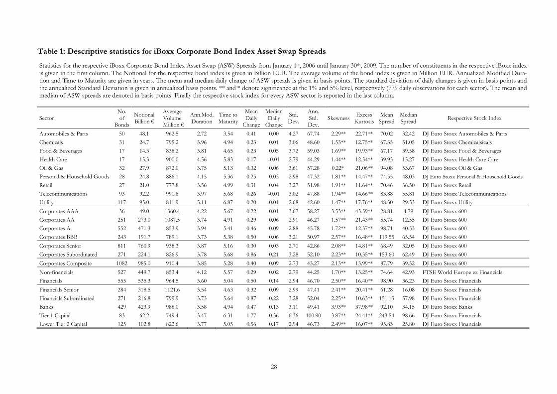
Table 1: Descriptive statistics for iBoxx Corporate Bond Index Asset Swap Spreads

Statistics for the respective iBoxx Corporate Bond Index Asset Swap (ASW) Spreads from January 1st, 2006 until January 30th, 2009. The number of constituents in the respective iBoxx index is given in the first column. The Notional for the respective bond index is given in Billion EUR. The average volume of the bond index is given in Million EUR. Annualized Modified Dura-tion and Time to Maturity are given in years. The mean and median daily change of ASW spreads is given in basis points. The standard deviation of daily changes is given in basis points and the annualized Standard Deviation is given in annualized basis points. ** and * denote significance at the 1% and 5% level, respectively (779 daily observations for each sector). The mean and median of ASW spreads are denoted in basis points. Finally the respective stock index for every ASW sector is reported in the last column.

Sector

No. of

Bonds

Notional Billion €

Average Volume Million €

Ann.Mod. Duration

Time to Maturity

Mean Daily

Change

Median Daily

Change

Std. Dev.

Ann. Std. Dev.

Skewness Excess Kurtosis

Mean Spread

Median Spread Respective Stock Index

Automobiles & Parts 50 48.1 962.5 2.72 3.54 0.41 0.00 4.27 67.74 2.29** 22.71** 70.02 32.42 DJ Euro Stoxx Automobiles & Parts Chemicals 31 24.7 795.2 3.96 4.94 0.23 0.01 3.06 48.60 1.53** 12.75** 67.35 51.05 DJ Euro Stoxx Chemicalsicals Food & Beverages 17 14.3 838.2 3.81 4.65 0.23 0.05 3.72 59.03 1.69** 19.93** 67.17 39.58 DJ Euro Stoxx Food & Beverages Health Care 17 15.3 900.0 4.56 5.83 0.17 -0.01 2.79 44.29 1.44** 12.54** 39.93 15.27 DJ Euro Stoxx Health Care Care Oil & Gas 32 27.9 872.0 3.75 5.13 0.32 0.06 3.61 57.28 0.22* 21.06** 94.08 53.67 DJ Euro Stoxx Oil & Gas Personal & Household Goods 28 24.8 886.1 4.15 5.36 0.25 0.03 2.98 47.32 1.81** 14.47** 74.55 48.03 DJ Euro Stoxx Personal & Household Goods Retail 27 21.0 777.8 3.56 4.99 0.31 0.04 3.27 51.98 1.91** 11.64** 70.46 36.50 DJ Euro Stoxx Retail Telecommunications 93 92.2 991.8 3.97 5.68 0.26 -0.01 3.02 47.88 1.94** 14.66** 83.88 55.81 DJ Euro Stoxx Telecommunications Utility 117 95.0 811.9 5.11 6.87 0.20 0.01 2.68 42.60 1.47** 17.76** 48.30 29.53 DJ Euro Stoxx Utility Corporates AAA 36 49.0 1360.4 4.22 5.67 0.22 0.01 3.67 58.27 3.53** 43.59** 28.81 4.79 DJ Euro Stoxx 600 Corporates AA 251 273.0 1087.5 3.74 4.91 0.29 0.06 2.91 46.27 1.57** 21.43** 55.74 12.55 DJ Euro Stoxx 600 Corporates A 552 471.3 853.9 3.94 5.41 0.46 0.09 2.88 45.78 1.72** 12.37** 98.71 40.53 DJ Euro Stoxx 600 Corporates BBB 243 191.7 789.1 3.73 5.38 0.50 0.06 3.21 50.97 2.57** 16.48** 119.55 65.54 DJ Euro Stoxx 600 Corporates Senior 811 760.9 938.3 3.87 5.16 0.30 0.03 2.70 42.86 2.08** 14.81** 68.49 32.05 DJ Euro Stoxx 600 Corporates Subordinated 271 224.1 826.9 3.78 5.68 0.86 0.21 3.28 52.10 2.23** 10.35** 153.60 62.49 DJ Euro Stoxx 600 Corporates Composite 1082 985.0 910.4 3.85 5.28 0.40 0.09 2.73 43.27 2.13** 13.99** 87.79 39.52 DJ Euro Stoxx 600 Non-financials 527 449.7 853.4 4.12 5.57 0.29 0.02 2.79 44.25 1.70** 13.25** 74.64 42.93 FTSE World Europe ex Financials Financials 555 535.3 964.5 3.60 5.04 0.50 0.14 2.94 46.70 2.50** 16.40** 98.90 36.23 DJ Euro Stoxx Financials Financials Senior 284 318.5 1121.6 3.54 4.63 0.32 0.09 2.99 47.41 2.41** 20.41** 61.28 16.08 DJ Euro Stoxx Financials Financials Subordinated 271 216.8 799.9 3.73 5.64 0.87 0.22 3.28 52.04 2.25** 10.63** 151.13 57.98 DJ Euro Stoxx Financials Banks 429 423.9 988.0 3.58 4.94 0.47 0.13 3.11 49.41 3.93** 37.98** 92.10 34.15 DJ Euro Stoxx Banks Tier 1 Capital 83 62.2 749.4 3.47 6.31 1.77 0.36 6.36 100.90 3.87** 24.41** 243.54 98.66 DJ Euro Stoxx Financials Lower Tier 2 Capital 125 102.8 822.6 3.77 5.05 0.56 0.17 2.94 46.73 2.49** 16.07** 95.83 25.80 DJ Euro Stoxx Financials

29

Figure 1: Sample Asset Swap (ASW) spreads stratified by industry sectors This table presents the development of ASW spreads for ten selected industry sectors included in our sample, from January, 1st 2006 until January, 30th 2009. ASW spreads are in basis points (left scale).

0

50

100

150

200

250

300

350

400

450

02.01.2006 02.07.2006 02.01.2007 02.07.2007 02.01.2008 02.07.2008 02.01.2009

Ass

et S

wap

Spr

eads

in

basi

s po

ints

Automobiles & Parts

Chemicals

Food & Beverage

Health Care

Oil & Gas

Personal & Household Goods

Retail

Telecommunications

Utility

Financials

30

Table 2: OLS results for determinants of Asset Swap Spreads Results of regressing daily changes in European iBoxx Corporate Bond index Asset Swap (ASW) spreads on determinants from equation 1: ΔASWt−1 is the lagged ASW spread change, ΔStock return represents the daily returns of the respective stock index, ΔVStoxx is the change in the VStoxx volatility index, ΔIR− Level denotes the change in the level of the swap curve, and ΔSwap Spread is the difference of the interest rate swap and the German government bond yield curve. Regression coefficients and corresponding t-statistics (in parentheses) are reported. We use a Newey-West consistent estimate of the covariance matrix to control for autocorrelation and heteroscedasticity. ** and * denote significance at the 1% and 5% level, respectively (779 daily observations – from January 1st, 2006 until January 30th, 2009).

const. ΔASWt-1 Stock return ΔVStoxx ΔIR-Level ΔSwap Spread Adj. R2 Automobiles & Parts

0.2615 0.3068* 0.9210 0.3794** -3.7011* 19.7132* 0.195 (1.92) (2.26) (0.17) (3.60) (-2.47) (2.01)

Chemicals 0.24 -0.0926 -0.7344 0.2196* -2.9816 8.6772 0.078

(2.03) (-1.05) (-0.08) (2.02) (-1.94) (1.16) Food & Beverages

0.2330 -0.0439 8.6440 0.3856** -2.4384 10.7061 0.074 (1.54) (-0.47) (0.47) (3.44) (-1.68) (1.20)

Health Care 0.1791 -0.1090 5.2131 0.2657** -2.0438 9.0762 0.086 (1.74) (-1.07) (0.34) (3.30) (-1.62) (1.27)

Oil & Gas 0.3016 -0.0116 -24.0346 0.1687 -2.9204 19.9049 0.110 (2.12) (-0.13) (-1.11) (0.82) (-1.88) (1.59)

Personal & Household Goods 0.2575 -0.0747 9.3766 0.2160* -2.9069* 11.2291 0.066 (2.28) (-0.85) (0.94) (2.40) (-2.53) (1.68)

Retail 0.2969 0.0085 7.5184 0.2395** -2.5535 14.1902 0.055 (2.23) (0.10) (0.47) (3.22) (-1.67) (1.63)

Telecommunications 0.2284 0.0592 -1.0540 0.2379** -2.4909 11.6075 0.073 (2.05) (0.50) (-0.06) (3.42) (-1.75) (1.87)

Utility 0.2366 -0.1510 -22.2952* 0.0167 -2.7670* 0.7191 0.080 (2.44) (-1.59) (-2.03) (0.17) (-2.53) (0.11)

Corporates AAA 0.1387 0.2365** -5.3751 0.2459 -1.2295 3.1947* 0.145 (1.00) (2.95) (-0.18) (1.58) (-0.90) (2.10)

Corporates AA 0.2549 0.0265 -17.7064 0.1351 -2.8248** 20.9809 0.118 (2.52) (0.29) (-1.21) (1.86) (-2.60) (1.63)

Corporates A 0.3890 0.0804 -34.5794* 0.0438 -2.3197 19.7208* 0.125 (3.93) (0.73) (-1.98) (0.56) (-1.75) (2.11)

Corporates BBB 0.4071 0.1280 -31.5625 0.1004 -1.9036 19.5567* 0.114 (3.80) (1.00) (-1.68) (1.04) (-1.09) (2.56)

Corporates Senior 0.2652 0.0263 -22.1838 0.1375* -2.2001 17.6829 0.129 (2.86) (0.24) (-1.50) (2.03) (-1.78) (1.77)

Corporates Subordinated 0.5975 0.2628** -37.7510* -0.0169 -2.4047 27.9731* 0.180 (4.96) (2.71) (-2.02) (-0.19) (-1.73) (2.42)

Corporates Composite 0.3439 0.0605 -2.6193 0.1048 -2.3592 1.9791 0.137 (3.68) (0.55) (-1.77) (1.66) (-1.91) (1.94)

Non-financials 0.2658 0.0274 -5.0430 0.1935* -2.5934* 12.1330 0.086 (2.59) (0.21) (-0.65) (2.44) (-2.07) (1.58)

Financials 0.3831 0.1745 -5.9668 0.1908** -2.7554* 31.9844* 0.176 (4.05) (1.52) (-0.63) (2.88) (-2.22) (2.35)

Financials Senior 0.2358 0.1749 -3.9140 0.2298** -2.3897* 34.7900* 0.180 (2.63) (1.40) (-0.41) (3.00) (-2.03) (2.30)

Financials Subordinated 0.6127 0.2642** -10.3032 0.1044 -3.0703* 29.5229* 0.172 (5.01) (2.77) (-0.83) (1.31) (-2.17) (2.44)

Banks 0.3983 0.1096 -0.2551 0.2195** -2.9245* 27.7989* 0.122 (3.60) (1.22) (-0.02) (2.86) (-2.46) (2.30)

Tier 1 Capital 0.7897 0.5297** -71.2776 -0.1031 0.9116 34.9503 0.350 (4.51) (6.30) (-1.85) (-0.38) (0.38) (1.92)

Lower Tier 2 Capital 0.4981 0.0626 -24.5580 0.0546 -3.2000* 15.4047 0.094 (4.54) (0.54) (-1.62) (0.68) (-2.48) (1.66)

31

Figure 2: The iBoxx Corporates Composite Asset Swap (ASW) Spread and its determinants Left hand scale: Determinants of Asset Swap spreads. Right hand scale: Asset Swap spread for the iBoxx Corporates Composite index. All series are normalized to start at 100.

0

50

100

150

200

250

300

350

400

450

50

70

90

110

130

150

170

190

210

02.01.2006 02.07.2006 02.01.2007 02.07.2007 02.01.2008 02.07.2008 02.01.2009

Euro Stoxx 600

Vstoxx

Interest Rates Level (PCA - based)

Swap Spread

ASW of iBoxx Corporates Composite

32

Figure 3: Evolution of OLS regression coefficients for stock market returns This figure presents the evolution of regression coefficients of the stock index variable in model (1). For reasons of brevity we only show the Corporates Senior and the Corporates Subordinated sector. The estimates are based on a rolling window of the last 100 observations.

-140

-120

-100

-80

-60

-40

-20

0

23.05.06 23.11.06 23.05.07 23.11.07 23.05.08 23.11.08

Corporates Senior

Corporates Subordinated

33

Table 3: Chow breakpoint test Rolling Chow breakpoint test for the whole sample, excluding the first and last 100 observations. The table provides the percentage of trading days the null hypothesis of no structural break can be rejected under the specified confidence level.

1% Level 5% Level 10% Level Automobiles & Parts 70.34% 89.14% 95.69% Chemicals 10.69% 48.79% 66.03% Food & Beverages 0.69% 16.38% 29.14% Health Care 0.00% 9.48% 39.48% Oil & Gas 61.21% 85.00% 96.55% Personal & Household Goods 13.28% 52.41% 68.45% Retail 23.62% 58.10% 73.79% Telecommunications 11.21% 49.31% 65.52% Utility 9.83% 31.55% 60.17% Corporates AAA 27.24% 45.86% 68.97% Corporates AA 42.07% 72.59% 88.62% Corporates A 85.00% 94.66% 98.28% Corporates BBB 80.17% 91.03% 96.03% Corporates Senior 66.72% 87.24% 95.86% Corporates Subordinated 96.03% 100.00% 100.00% Corporates Composite 81.72% 93.97% 97.76% Non-financials 52.41% 72.93% 85.17% Financials 88.97% 97.41% 99.66% Financials Senior 73.10% 95.52% 98.28% Financials Subordinated 96.21% 100.00% 100.00% Banks 78.28% 91.90% 96.03% Tier 1 Capital 99.48% 100.00% 100.00% Lower Tier 2 Capital 85.17% 95.86% 98.62%

34

Table 4: Results of Markov switching regressions Results for the Markov switching regression of changes in European iBoxx Corporate Bond index Asset Swap (ASW) spreads on theoretical determinants. Regression coefficients and corresponding z-statistics (in parentheses) are reported. We use a Newey-West consistent estimate of the covariance matrix to control for autocorrelation and heteroscedasticity. The theoretical determi-nants are: lagged ASW changes (ΔASWt−1), daily stock index returns (Stock return), the change in the VStoxx volatility index (ΔVStoxx), the change in the level of the swap curve (ΔIR − Level), and the difference of the swap and the German government yield curve (ΔSwap Spread). The sample consists of 779 daily observations – from January 1st, 2006 until January 30th, 2009. Re-gime 1 and 2 represent the volatile and tranquil market regime, respectively. The regime dependent residual standard deviation - denoted as Std. Dev. - is quoted in annualized basis points. pii gives the probability of staying in the respective regime. The regime dependent State Duration is quoted in days. ** and * denote significance at the 1% and 5% level, respectively.

const. ΔASWt-1 Stock return ΔVStoxx ΔIR-Level ΔSwap

Spread Std. Dev. pii State

Duration Automobiles & Parts

Regime 1 0.0087** 0.3532** -1.2998 0.4315** -5.9386** 32.6251** 110.8669 0.8705 7.72 (3.04) (6.65) (-0.44) (8.60) (-3.36) (3.53)

Regime 2 0.0001 -0.0945** -11.6288** -0.0913 -2.1758** 1.1762 16.2370 0.9551 22.26 (0.10) (-4.49) (-2.65) (-1.76) (-4.17) (0.54)

Chemicals Regime 1 0.0071 -0.0790 8.0676 0.2692 -4.9517 16.6294 85.2649 0.9237 13.11

(1.06) (-0.58) (0.15) (1.62) (-0.52) (0.43) Regime 2 0.0008 -0.1514 -13.7743 -0.0012 -1.7942** 0.9236 17.4629 0.9728 36.74

(0.20) (-0.71) (-0.67) (-0.02) (-3.61) (0.06) Food & Beverages

Regime 1 0.0054 0.0025 -20.9444** 0.3224** -3.7208** 21.7357* 102.9351 0.8822 8.49 (1.08) (0.07) (-3.64) (6.00) (-4.15) (2.78)

Regime 2 0.0007* -0.1369* -23.2275** -0.1020** -1.2169 -2.9104 14.9158 0.9556 22.54 (2.02) (-2.07) (-6.55) (-3.26) (-2.21) * (-0.38)

Health Care Regime 1 0.0055** -0.0890 6.7733 0.2910** -3.7628** 15.9705 75.1542 0.8744 7.96

(3.34) (-1.37) (0.30) (4.21) (-3.47) (1.17) Regime 2 0.0001 -0.1787* -10.8026 -0.0061 -0.6915 1.3854 13.7207 0.9505 20.21

(1.20) (-2.21) (-0.46) (-0.04) (-1.63) (0.32) Oil & Gas

Regime 1 0.0108 0.0344 -20.3847** 0.2052** -6.1498** 41.2796** 112.5837 0.9197 12.45 (1.55) (0.94) (-3.32) (4.30) (-2.83) (4.25)

Regime 2 0.0012 -0.1990* -15.0015 -0.0278 -2.8551* 0.7606 22.6032 0.9827 57.92 (1.98) (-2.44) (-1.17) (-0.41) (-2.26) (0.38)

Personal & Household Goods Regime 1 0.0089* -0.0870 23.8413 0.2644* -4.8654* 17.2511 78.8854 0.8963 9.64

(2.38) (-1.39) (1.05) (2.48) (-2.40) (1.50) Regime 2 -0.0001 -0.0677* -9.8711* -0.0226 -1.1003** 3.2185 14.3114 0.9563 22.87

(-0.35) (-2.02) (-2.10) (-0.51) (-2.68) (1.02) Retail

Regime 1 0.0094* 0.0077 20.2265 0.2877* -3.5028 22.7682 90.9326 0.8829 8.54 (2.01) (0.11) (0.93) (2.35) (-1.71) (1.82)

Regime 2 0.0005 -0.0733* -12.3934** -0.0016 -1.8851** 0.5360 15.6158 0.9561 22.77 (1.16) (-2.28) (-3.14) (-0.04) (-4.70) (0.18)

Telecommunications Regime 1 0.0063 0.0731 -2.5538 0.2558 -3.9102 18.9734 81.7654 0.9167 12.01

(1.51) (1.05) (-0.10) (1.88) (-1.83) (1.46) Regime 2 0.0005 -0.0150 -2.4146 0.0375 -1.4312** 3.2672 16.7733 0.9687 31.99

(0.95) (-0.41) (-0.51) (0.91) (-3.25) (1.03) Utility

Regime 1 0.0078 -0.1778** -22.6610** 0.0412 -4.9167* 0.1832 75.7516 0.9146 11.70 (1.30) (-2.86) (-5.52) (1.30) (-2.43) (0.04)

Regime 2 0.0004* -0.1468** -17.0674** -0.0436 -1.0210 -0.3179 15.6115 0.9719 35.53 (2.45) (-5.70) (-2.84) (-0.75) (-0.97) (-0.45)

Corporates AAA Regime 1 0.0056 0.2873** 3.6822 0.2858 -3.2080 52.8956** 115.4664 0.9217 12.77

(1.30) (13.4) (0.03) (0.65) (-0.85) (3.27) Regime 2 0.0008** -0.2699** -17.7525* -0.1043* -1.5183** -2.8673 16.8719 0.9827 57.82

(2.86) (-3.23) (-2.17) (-2.43) (-2.93) (-0.81) Corporates AA

Regime 1 0.0067** 0.0579 -12.4094 0.1690** -4.7488** 36.1258** 71.1397 0.8873 8.88 (4.27) (1.16) (-1.15) (4.60) (-5.72) (3.49)

Regime 2 0.0005* -0.1470 -14.7228 -0.0247 -1.6224** -0.9396 12.3050 0.9454 18.31 (2.06) (-0.70) (-0.85) (-0.33) (-9.36) (-0.26)

35

Table 4 (cont.): Result of Markov switching regressions

const. ΔASWt-1 Stock return ΔVStoxx ΔIR-Level ΔSwap

Spread Std. Dev. pii State

Duration Corporates A Regime 1 0.0106** 0.0798 -30.1514* 0.0993 -3.8684* 32.1492** 73.1683 0.9057 10.60

(3.60) (1.79) (-2.53) (1.71) (-2.45) (5.98) Regime 2 0.0013** -0.0497 -38.5933** -0.2036* -1.5196** 2.5043 14.7798 0.9625 26.66

(3.12) (-0.17) (-4.37) (-2.62) (-4.44) (0.71) Corporates BBB Regime 1 0.0129* 0.1064 -30.6951 0.1754 -3.0372 27.2616* 85.3892 0.9008 10.08

(2.69) (1.75) (-1.22) (1.26) (-1.40) (2.31) Regime 2 0.0011* 0.0372 -37.6421** -0.2341** -1.8140** 5.6972 16.2048 0.9641 27.88

(2.21) (1.02) (-4.52) (-3.98) (-3.82) (1.95) Corporates Senior Regime 1 0.0072* 0.0533 -22.9137 0.1612 -3.5763 29.7785** 68.5249 0.9156 11.85

(2.19) (0.82) (-1.04) (1.11) (-1.96) (3.65) Regime 2 0.0006 -0.1486** -21.3212** -0.1119* -1.5390** 1.9404 13.2823 0.9659 29.31

(1.57) (-3.85) (-3.43) (-2.40) (-3.99) (0.72) Corporates Subordinated Regime 1 0.0125** 0.2536** -25.0488 0.0315 -3.7312* 38.9976** 65.7289 0.9514 20.58

(4.44) (5.81) (-1.36) (0.23) (-2.40) (7.41) Regime 2 0.0015** -0.1271** -57.1431** -0.2574** -0.9427 3.5802 13.4608 0.9593 24.58

(3.21) (-3.65) (-6.29) (-4.06) (-1.92) (1.16) Corporates Composite Regime 1 0.0095** 0.0632 -21.1703 0.1647 -4.0552* 32.0181** 67.7992 0.9150 11.76

(2.95) (1.05) (-0.97) (1.05) (-2.21) (4.24) Regime 2 0.0009* -0.0626 -30.6173** -0.1553** -1.4657** 3.1737 13.9057 0.9652 28.75

(2.29) (-1.66) (-4.95) (-3.79) (-3.88) (1.12) Non-financials Regime 1 0.0079* 0.0430 -11.6668 0.2103 -3.7366 17.7671 73.4352 0.9167 12.01

(2.33) (0.54) (-0.75) (1.75) (-1.89) (1.49) Regime 2 0.0004 -0.1578** -2.4209 -0.0345 -1.6864** 2.3315 14.2543 0.9674 30.65

(0.80) (-2.74) (-0.57) (-0.64) (-3.78) (0.91) Financials Regime 1 0.0085 0.2071* 4.5976 0.2377 -3.9571* 48.7543** 61.6147 0.9245 13.24

(1.81) (2.33) (0.35) (1.98) (-2.29) (3.14) Regime 2 0.0008 -0.1671 -21.7275* -0.0940 -1.4653 1.7697 11.6361 0.9471 18.91

(0.92) (-1.49) (-2.03) (-0.97) (-1.11) (0.34) Financials Senior Regime 1 0.0071* 0.2167** 8.1620 0.3798* -4.7083** 60.5424** 72.1853 0.8483 6.59

(2.24) (2.95) (0.64) (2.19) (-3.00) (4.09) Regime 2 0.0007 -0.1514 1.0613 0.0671** -1.7790** 2.2155 12.6594 0.9395 16.54

(1.34) (-1.24) (0.76) (3.15) (-6.43) (0.57) Financials Subordinated Regime 1 0.0130** 0.2547** 2.8750 0.1561 -4.5369** 42.3740** 65.8223 0.9520 20.85

(4.69) (4.85) (0.24) (1.59) (-2.91) (4.91) Regime 2 0.0013* -0.1265* -39.6987** -0.1838* -1.0896 3.0546 13.2163 0.9599 24.92

(2.51) (-2.38) (-5.11) (-2.37) (-1.96) (0.86) Banks Regime 1 0.0095** 0.1238* 12.2365 0.2895* -4.4491* 44.2449** 70.7211 0.9091 11.00

(2.78) (2.05) (0.73) (2.20) (-2.49) (6.25) Regime 2 0.0009* -0.1434** -17.7257** -0.0974** -1.6054** 1.2231 12.0942 0.9450 18.20

(2.37) (-4.10) (-5.28) (-2.72) (-4.21) (0.43) Tier 1 Capital Regime 1 0.0180 0.5154** -65.3662** -0.0783 0.7569 47.8202** 118.6375 0.9329 14.90

(1.35) (8.7) (-2.85) (-0.51) (0.26) (7.39) Regime 2 0.0014 -0.0646 -74.4322 -0.3402 -0.0774 2.1095 17.1272 0.9491 19.65

(0.68) (-0.96) (-1.39) (-0.65) (-0.06) (1.11) Lower Tier 2 Capital Regime 1 0.0106** 0.0555 -14.3953 0.0985** -4.7018 22.6938** 63.8301 0.9510 20.39

(3.21) (0.76) (-1.55) (3.56) (-1.77) (5.71) Regime 2 0.0010** -0.1613** -35.8535** -0.1566 -0.9703* 0.7634 11.6346 0.9609 25.60

(4.22) (-2.71) (-2.97) (-1.52) (-2.63) (0.52)

36

Table 5: Test for equality of determinants in both regimes Results of Likelihood Ratio (LR) tests of equality of all coefficients in both regimes (H0: No switching in all variables). LR represents the likelihood ratio test statistic. Corresponding p-values are presented in the last column.

LR p-value

Automobiles & Parts 51.363 0.000 Chemicals 11.842 0.037 Food & Beverages 22.754 0.000 Health Care 18.663 0.002 Oil & Gas 25.864 0.000 Personal & Household Goods 18.203 0.003 Retail 14.934 0.011 Telecommunications 14.997 0.010 Utility 11.348 0.045 Corporates AAA 53.369 0.000 Corporates AA 32.940 0.000 Corporates A1 33.420 0.000 Corporates BBB 30.852 0.000 Corporates Senior 36.033 0.000 Corporates Subordinated 82.552 0.000 Corporates Composite 39.948 0.000 Non-financials 28.125 0.000 Financials 65.799 0.000 Financials Senior 57.524 0.000 Financials Subordinated 88.267 0.000 Banks 50.427 0.000 Tier 1 Capital 110.791 0.000 Lower Tier 2 Capital 49.998 0.000

37

Table 6: Regime specific moments of Asset Swap Spreads This table compares the regime specific moments (mean, skewness and kurtosis) of the asset swap spread changes. The value of the mean is reported in basis points. The second column presents the percentage of time sample indices spend in Regime 1 (volatile regime).

Regime 1 Regime 2

High volatility regime Low volatility regime

Time in regime 1 Mean Skewness Excess

kurtosis Mean Skewness Excess kurtosis

Automobiles & Parts 17.8% 2.27 0.59 2.31 0.01 0.08 1.29 Chemicals 26.8% 0.76 0.66 2.00 0.04 0.33 0.54 Food & Beverages 25.9% 0.75 0.73 3.54 0.06 0.02 0.55 Health Care 27.9% 0.55 0.64 1.91 0.03 0.31 0.56 Oil & Gas 16.3% 1.80 -0.42 2.95 0.04 0.06 0.97 Personal & Household Goods 27.3% 0.92 0.73 2.36 0.00 0.25 0.36 Retail 24.6% 1.12 0.73 1.00 0.05 0.25 0.83 Telecommunications 25.0% 0.95 0.82 2.22 0.03 0.21 0.34 Utility 22.6% 0.74 0.56 2.96 0.05 0.26 0.49 Corporates AAA 18.1% 0.97 1.46 6.75 0.06 0.23 1.23 Corporates AA 28.5% 0.92 0.60 4.99 0.04 0.36 0.95 Corporates A 26.8% 1.33 0.59 1.82 0.14 0.42 0.78 Corporates BBB 25.3% 1.63 1.03 2.51 0.13 0.46 0.67 Corporates Senior 28.0% 0.95 0.89 2.60 0.05 0.41 0.73 Corporates Subordinated 43.9% 1.84 1.17 3.22 0.10 0.34 0.59 Corporates Composite 27.3% 1.19 0.87 2.29 0.10 0.44 0.64 Non-financials 26.8% 0.98 0.64 2.02 0.04 0.37 0.66 Financials 39.3% 1.16 1.34 5.06 0.08 0.29 0.86 Financials Senior 25.7% 1.10 1.00 3.60 0.06 0.20 1.18 Financials Subordinated 48.1% 1.74 1.26 3.88 0.08 0.25 0.81 Banks 36.6% 1.18 2.25 13.20 0.07 0.30 0.88 Tier 1 Capital 44.9% 3.85 2.37 9.85 0.09 0.42 0.81

Lower Tier 2 Capital 39.0% 1.30 1.35 5.19 0.09 0.59 2.45

38

Figure 4: Regime probabilities and Asset Swap (ASW) Spreads Estimated probability of being in the volatile regime - based on the filtered probability (grey bars and left hand scale: a value of 100% indicates being in the volatile regime, a value of zero being in the tranquil regime) and squared changes in the iBoxx Corporate Composite ASW spread (black line and right hand scale). The events are: (1) House price stagnation, (2) Ameriquest, (3) Credit markets start to freeze, (4) Bear Stearns, (5) Freddie Mac and Fannie Mae, (6) Lehman Brothers, and (7) Citigroup.

0

50

100

150

200

250

300

350

400

450

0%

10%

20%

30%

40%

50%

60%

70%

80%

90%

100%

04.01.2006 04.07.2006 04.01.2007 04.07.2007 04.01.2008 04.07.2008 04.01.2009

1 2 3 4 5 6 7

39

Table 7: Logit Models This Table presents the α1 coefficients from the logit regressions (see equation 11) with t-statistics (in parentheses) and R2 (in square brackets). We use a Huber-White consistent estimate of the covariance matrix to control for auto-correlation and heteroscedasticity. The theoretical determinants are: lagged squared ASW changes (∆ASWt−1

2 ), lagged ASW changes (ΔASWt−1), lagged daily stock index returns (ΔStock return𝑡−1), lagged change in the VStoxx volatility index (ΔVStoxxt−1), lagged change in the level of the swap curve (ΔIR − Level𝑡−1), and lagged changes in the differ-ence of the swap and the German government yield curve (ΔSwap Spread𝑡−1).

ΔASW2t-1 ΔASWt-1 Stock returnt-1 ΔVStoxxt-1 ΔIR-Levelt-1 ΔSwap

Spreadt-1 Automobiles & Parts

0.0215 0.0592* -3.7964 0.0296 -1.6002* 4.6729 (1.3180) (2.1888) (-0.7337) (0.5576) (-2.0504) (0.9468) [0.0963] [0.0115] [0.0019] [0.0008] [0.0074] [0.0021]

Chemicals 0.3505** 0.0662 -12.2542 0.0264 -1.3362 0.1193 (10.103) (1.7370) (-1.7548) (0.5267) (-1.7605) (0.0264) [0.4121] [0.0072] [0.0072] [0.0006] [0.0053] [0.0000]

Food & Beverages 0.1033 0.0648* -15.3480 0.0661 -1.3118 4.8336 (1.1110) (2.0746) (-1.9482) (1.4352) (-1.7492) (1.0914) [0.2002] [0.0100] [0.0072] [0.0040] [0.0051] [0.0023]

Health Care 0.4450** 0.0860* -9.5170 0.0164 -1.0351 2.8991 (10.178) (2.1145) (-1.2537) (0.3435) (-1.4359) (0.6898) [0.4074] [0.0099] [0.0032] [0.0002] [0.0032] [0.0008]

Oil & Gas 0.1564** 0.1143* -9.0381 0.0570 -1.6222 5.3706 (10.380) (2.2407) (-0.9860) (0.8961) (-1.5414) (0.8895) [0.4072] [0.0268] [0.0047] [0.0030] [0.0068] [0.0027]

Personal & Household Goods 0.5183** 0.0998** -14.1169* 0.0381 -0.8799 1.8637 (10.972) (2.6050) (-1.9619) (0.8170) (-1.2257) (0.4393) [0.4659] [0.0152] [0.0079] [0.0013] [0.0023] [0.0003]

Retail 0.4002** 0.0915** -3.5135 0.0405 -1.0232 -0.0906 (9.8899) (2.6755) (-0.4828) (0.8210) (-1.3132) (-0.0194) [0.4777] [0.0161] [0.0004] [0.0015] [0.0031] [0.0000]

Telecommunications 0.4030** 0.0793* -13.2334 0.0412 -1.6271* 2.3138 (9.1460) (2.1298) (-1.6666) (0.8575) (-2.1035) (0.5159) [0.4471] [0.0101] [0.0057] [0.0015] [0.0078] [0.0005]

Utility 0.4437** 0.0963* -8.2295 0.0398 -0.9558 2.8419 (11.264) (1.9925) (-1.0364) (0.7856) (-1.1490) (0.5848) [0.4465] [0.0114] [0.0031] [0.0014] [0.0026] [0.0007]

Corporates AAA 0.2820** 0.0580 -12.4132 0.0249 -1.9375* 2.0945 (8.4606) (1.6561) (-1.2783) (0.3708) (-2.0579) (0.3538) [0.4021] [0.0086] [0.0058] [0.0005] [0.0105] [0.0004]

Corporates AA 0.4806** 0.1077** -16.7895* 0.0724 -0.7876 0.1266 (7.3090) (2.5942) (-2.4332) (1.8124) (-1.1660) (0.0326) [0.3798] [0.0157] [0.0112] [0.0048] [0.0019] [0.0000]

40

Table 7 (cont.): Logit Models

ΔASW2t-1 ΔASWt-1 Stock returnt-1 ΔVStoxxt-1 ΔIR-Levelt-1 ΔSwap Spreadt-1 Corporates A

0.4426** 0.1512** -10.4261 0.0206 -0.7296 0.6953 (10.785) (3.4699) (-1.4730) (0.4458) (-0.9945) (0.1627) [0.4540] [0.0307] [0.0043] [0.0003] [0.0016] [0.0000]

Corporates BBB 0.3865** 0.1426** -10.2304 0.0181 -0.2489 -0.1028 (9.1046) (3.8020) (-1.3968) (0.3614) (-0.3224) (-0.0224) [0.4488] [0.0346] [0.0041] [0.0003] [0.0001] [0.0000]

Corporates Senior 0.5321** 0.1186** -14.6936* 0.0434 -0.9136 0.5897 (10.959) (2.8624) (-2.0244) (0.9708) (-1.2660) (0.1396) [0.4330] [0.0175] [0.0086] [0.0017] [0.0025] [0.0000]

Corporates Subordinated 0.4466** 0.1824** -10.8897* 0.0298 -1.0134 0.4952 (8.9094) (5.7129) (-2.0384) (0.9239) (-1.7635) (0.1587) [0.3776] [0.0473] [0.0049] [0.0008] [0.0032] [0.0000]

Corporates Composite 0.4929** 0.1496** -14.5235* 0.0551 -0.8982 0.9719 (10.416) (3.4645) (-2.0490) (1.3099) (-1.2496) (0.2334) [0.4291] [0.0272] [0.0084] [0.0028] [0.0024] [0.0000]

Non-financials 0.5471** 0.1204** -9.6836* 0.0272 -1.3270 2.5513 (10.476) (2.8247) (-2.0118) (0.5743) (-1.7852) (0.5834) [0.4717] [0.0191] [0.0080] [0.0006] [0.0052] [0.0006]

Financials 0.1577 0.1302** -8.0129 0.0381 -0.5163 0.9177 (1.0619) (3.4984) (-1.7909) (1.1008) (-0.8573) (0.2741) [0.1566] [0.0222] [0.0047] [0.0013] [0.0008] [0.0000]

Financials Senior 0.1285 0.1014** -13.4546* 0.0806 -0.2518 1.9505 (1.3689) (2.6230) (-2.4337) (1.8468) (-0.3383) (0.4784) [0.1756] [0.0159] [0.0124] [0.0060] [0.0001] [0.0003]

Financials Subordinated 0.4534** 0.1913** -5.6658 0.0104 -0.7220 0.2365 (8.5665) (5.7485) (-1.4263) (0.3127) (-1.2659) (0.0758) [0.3798] [0.0506] [0.0024] [0.0001] [0.0016] [0.0000]

Banks 0.5355** 0.1333** -10.3453* 0.0539 -0.3633 1.5944 (8.3182) (3.4855) (-2.2662) (1.5029) (-0.5814) (0.4554) [0.3873] [0.0232] [0.0082] [0.0027] [0.0004] [0.0002]

Tier 1 Capital 0.1082 0.1502** -10.2846 0.0208 -0.9716 2.5760 (1.7119) (5.8182) (-1.8359) (0.5906) (-1.6346) (0.7679) [0.2752] [0.0787] [0.0044] [0.0004] [0.0029] [0.0007]

Lower Tier 2 Capital 0.6208** 0.1542* -10.1723 0.0150 -0.4266 0.8332 (8.1869) (4.2409) (-1.8620) (0.4384) (-0.7336) (0.2600) [0.3931] [0.0287] [0.0043] [0.0002] [0.0005] [0.0000]

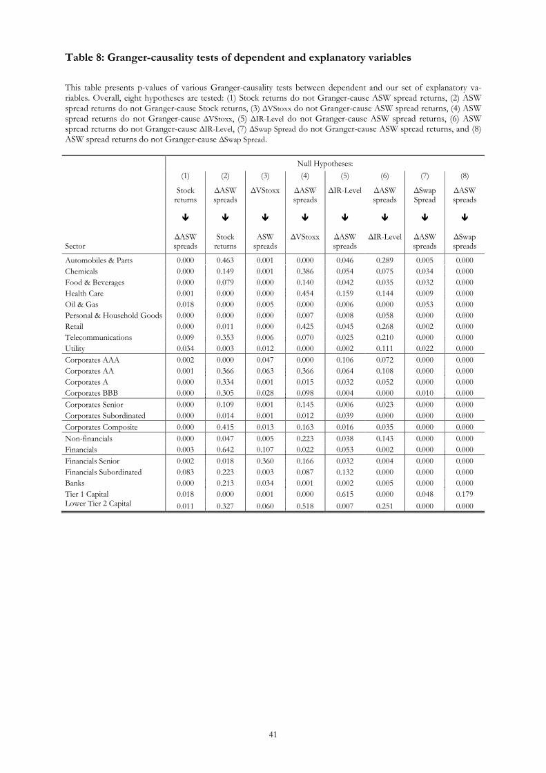
41

Table 8: Granger-causality tests of dependent and explanatory variables This table presents p-values of various Granger-causality tests between dependent and our set of explanatory va-riables. Overall, eight hypotheses are tested: (1) Stock returns do not Granger-cause ASW spread returns, (2) ASW spread returns do not Granger-cause Stock returns, (3) ΔVStoxx do not Granger-cause ASW spread returns, (4) ASW spread returns do not Granger-cause ΔVStoxx, (5) ΔIR-Level do not Granger-cause ASW spread returns, (6) ASW spread returns do not Granger-cause ΔIR-Level, (7) ΔSwap Spread do not Granger-cause ASW spread returns, and (8) ASW spread returns do not Granger-cause ΔSwap Spread.

Null Hypotheses:

Sector

(1)

Stock returns

ΔASW spreads

(2)

ΔASW spreads

Stock returns

(3)

ΔVStoxx

ASW spreads

(4)

ΔASW spreads

ΔVStoxx

(5)

ΔIR-Level

ΔASW spreads

(6)

ΔASW spreads

ΔIR-Level

(7)

ΔSwap Spread

ΔASW spreads

(8)

ΔASW spreads

ΔSwap spreads

Automobiles & Parts 0.000 0.463 0.001 0.000 0.046 0.289 0.005 0.000 Chemicals 0.000 0.149 0.001 0.386 0.054 0.075 0.034 0.000 Food & Beverages 0.000 0.079 0.000 0.140 0.042 0.035 0.032 0.000 Health Care 0.001 0.000 0.000 0.454 0.159 0.144 0.009 0.000 Oil & Gas 0.018 0.000 0.005 0.000 0.006 0.000 0.053 0.000 Personal & Household Goods 0.000 0.000 0.000 0.007 0.008 0.058 0.000 0.000 Retail 0.000 0.011 0.000 0.425 0.045 0.268 0.002 0.000 Telecommunications 0.009 0.353 0.006 0.070 0.025 0.210 0.000 0.000 Utility 0.034 0.003 0.012 0.000 0.002 0.111 0.022 0.000 Corporates AAA 0.002 0.000 0.047 0.000 0.106 0.072 0.000 0.000 Corporates AA 0.001 0.366 0.063 0.366 0.064 0.108 0.000 0.000 Corporates A 0.000 0.334 0.001 0.015 0.032 0.052 0.000 0.000 Corporates BBB 0.000 0.305 0.028 0.098 0.004 0.000 0.010 0.000 Corporates Senior 0.000 0.109 0.001 0.145 0.006 0.023 0.000 0.000 Corporates Subordinated 0.000 0.014 0.001 0.012 0.039 0.000 0.000 0.000 Corporates Composite 0.000 0.415 0.013 0.163 0.016 0.035 0.000 0.000 Non-financials 0.000 0.047 0.005 0.223 0.038 0.143 0.000 0.000 Financials 0.003 0.642 0.107 0.022 0.053 0.002 0.000 0.000 Financials Senior 0.002 0.018 0.360 0.166 0.032 0.004 0.000 0.000 Financials Subordinated 0.083 0.223 0.003 0.087 0.132 0.000 0.000 0.000 Banks 0.000 0.213 0.034 0.001 0.002 0.005 0.000 0.000 Tier 1 Capital 0.018 0.000 0.001 0.000 0.615 0.000 0.048 0.179 Lower Tier 2 Capital 0.011 0.327 0.060 0.518 0.007 0.251 0.000 0.000

European Asset Swap Spreads and the Credit Crisis · A further possible determinant of credit...

Documents

Transcript of European Asset Swap Spreads and the Credit Crisis · A further possible determinant of credit...