Ethanol-Blended Gasoline Policy and Ozone Pollution in Sao Paulo

Alberto Salvo and Yi Wang∗

January 16, 2017

Abstract

We examine four discontinuities in the ethanol content in blended gasoline fuel, mandatedby Brazil’s central government over the period 2010 to 2013, to test the joint hypotheses that(1) atmospheric ozone production in the Sao Paulo metropolitan area is limited by the volumeand reactivity of volatile organic compounds (“VOC-limited”), and (2) increased ethanol usein the gasoline-ethanol vehicle fleet leads to higher ozone concentrations in urban Sao Paulo’sambient air. We adopt a regression discontinuity design (RDD) and flexibly test each disconti-nuity separately. Our finding that ozone levels actually increased with ethanol penetration oneach of the four occasions is consistent with a recent empirical study that used different identi-fying variation, and contrasts with a modeling study of Sao Paulo’s atmosphere that predictedsignificant ozone abatement from hypothetical ethanol use. We find no significant relationshipbetween ethanol versus gasoline use and PM2.5 levels. Current tailpipe emissions standardsprescribe the exclusion of the mass of unburned ethanol that is emitted—our result suggeststhat this standard be reviewed. Following decades of VOC emissions control, urban areas inthe US and elsewhere that are currently VOC-limited may see ozone levels rise if and whenthey adopt mid-level ethanol gasoline blends, whether to meet the Renewable Fuel Standard orIntended Nationally Determined Contributions to abating fossil-fuel emissions agreed upon atCOP-21 in Paris.

Keywords: Ethanol, biofuels, gasoline blends, ozone, PM2.5, air pollution, emissions standards,regression discontinuity design, RDD, Renewable Fuel Standard, blend wall, gasoline content

JEL classification: I18, L52, L71, Q16, Q42, Q53

∗Alberto Salvo and Yi Wang, Department of Economics, National University of Singapore, 1 Arts Link, Singapore117570. Email: albertosalvo@nus.edu.sg and w.yi@u.nus.edu. We gratefully acknowledge numerous people fromANP, CBN Noticias, CET, CETESB, INMET and Raizen for generously sharing their data, archives and otherinformation. In particular, we thank Wagner Baptista, Wanessa Canellas, Cristina Costa, Alaor Dall’Antonia Jr,Fabio Henkes, Masayuki Kuromoto, Carlos Lacava, Dario Garcia Medeiros, Rui Cesar Melo, Clarice Aico Muramoto,Roseni dos Santos, Telma Paulino Senaubar and Mariza Tavares. We thank Sam Ritchey and Jiaxiu He for compilingthe GPS coordinates of road segments. AS acknowledges support from the Initiative for Sustainability and Energyat Northwestern University (ISEN), from the Dean’s Office at the Kellogg School of Management, NorthwesternUniversity, and from the Dean’s Office at the Faculty of Arts & Social Sciences, National University of Singaporeunder start-up grant R-122-000-187-133.

1 Introduction

In recent decades, effective emissions control policies, particularly of volatile organic compounds

(VOC), may have shifted the ozone production regime in urban atmospheres in the United States

and elsewhere, from the “VOC-saturated” to the “VOC-limited” regime. Under such atmospheric

conditions, further reductions in the volume and reactivity of VOC emissions can reduce the for-

mation of ozone, a secondary pollutant that at the ground level harms human health, whereas

reductions in nitrogen oxides (NOx) emissions can actually cause ozone concentrations to rise (Ja-

cob 1999). Conversely, under VOC-saturated (“VOC-insensitive” or “NOx-limited”) conditions,

ozone production is insensitive to variation in VOC emissions and increasing in NOx emissions.

Knowledge of the atmospheric ozone production regime, and how it may be changing over time,

is therefore critical to designing successful ozone control strategies. Such knowledge is not acquired

without cost, however, as evidenced by a large atmospheric modeling literature that studies the

chemistry of atmospheres over specific metropolitan areas or regions, and how its composition

evolves over the annual, weekly and daily cycles. Models build on our current understanding of

chemical and physical reactions of species in the atmosphere, and are based on often incomplete

inventories of anthropogenic and biogenic emissions, by chemical species over time and in space.

These computationally intensive differential-equation models are then used to predict how specific

emissions control policies, for example, changes in the mix or composition of fuels utilized in the

urban transport fleet, impact ambient pollutant concentrations, such as ozone (O3) and particulate

matter (PM). Madronich (2014) states: “uncertainties in numerical models often preclude firm

conclusions regarding the dominant control over ozone chemistry in a city” (p.397). The difficulty

in diagnosing the state of the local atmosphere is also suggested by the fact that, whereas decades

of pollution control have led to the abatement of urban pollutants such as carbon monoxide (CO),

NOx and PM, the record on ozone abatement is more mixed.

A case in point is the metropolis of Sao Paulo, in southeastern Brazil. Home to 20 million

people, the Sao Paulo metropolitan area combines 40 municipalities and accounts for one-fifth of

the country’s GDP. Over the 1980s and 1990s, the metropolis experienced a steady process of

deindustrialization, as factories moved inland or out of state. The economy today is dominated by

services, and power generation is mostly hydroelectric. With a mild climate that requires minimal

winter heating, the predominant source of anthropogenic emissions of ozone precursors—NOx, VOC

1

and CO—is road transport. The circulating fleet is comprised of 6 million passenger cars, burning a

mix of gasoline and ethanol that has varied over time, 1 million motorcycles predominantly powered

by gasoline, and 120,000 diesel buses and trucks. Both gasoline fuel—in fact a blend containing a 20

to 25% volumetric component of pure ethanol, thus referred to as E20/E25—and ethanol fuel—in

the form of E100—are universally available at the pump, one nozzle typically alongside the other.

Among regulated air pollutants, ozone often exceeds the standard (CETESB 2013) and is the one

species that did not exhibit a downward trend in the period 2000 to 2013 (Perez-Martinez et al.

2015).1

An atmospheric modeling study, calibrated to Sao Paulo using the available emissions data,

predicted that if all passenger cars were to run on ethanol (E100) rather than a combination of the

ethanol and blended gasoline (E20/E25) fuels that heterogeneous consumers purchase at retail, then

ozone levels would fall by up to 55% (Martins and Andrade 2008a). However, a recent empirical

(econometric) study found the opposite effect (Salvo and Geiger 2014). The study exploited drivers

of “flexible fuel” vehicles (FFVs) substituting between blended gasoline and ethanol as relative

prices fluctuated at the pump, and concluded that substitution into ethanol caused ozone levels to

rise. This single test suggested that modern-day Sao Paulo’s atmosphere is VOC-limited, by which

higher ozone levels associated with an increased ethanol fraction in the fuel mix was due either

to (1) higher reactivity of VOCs from ethanol relative to gasoline use, whether via combustion

or evaporation processes, and/or (2) lower NOx emissions from ethanol combustion relative to

gasoline.2 Salvo and Geiger’s empirical finding was consistent with a controversial atmospheric

modeling study that predicted that ozone levels would rise in Los Angeles, and elsewhere in the

US, were passenger cars to adopt E85 ethanol over E10 gasoline (respectively, ethanol and gasoline

fuels that are retailed in the US) (Jacobson 2007, Ginnebaugh et al. 2010).

This paper, based on four separate quasi-experiments, provides an important second empirical

test of the combined hypotheses that the Sao Paulo megacity’s atmosphere is VOC-limited and that

higher fractions of ethanol at the expense of gasoline in the light-vehicle fuel mix cause ozone levels

to rise. Rather than take as identifying variation FFV owners choosing either E20/E25 gasoline or

1Sao Paulo’s maximum daily 8-hour ozone standard is 140 µg/m3, or about 71 parts per billion (ppb). Sao PauloState Decree 59113, issued April 23, 2013, signals a long-run reduction to 100 µg/m3 (51 ppb), citing current scientificknowledge of the health damage of ozone. For comparison, the new (2015) US NAAQS for ozone is 70 ppb. The USEPA summarizes trends for the US as follows: “Nationally, average ozone levels declined in the 1980s, leveled off inthe 1990s, and showed a notable decline after 2002” (epa.gov/airtrends/ozone.html, accessed on May 10, 2016).

2Section 2 cites vehicle emissions standards legislation that allows carmakers to exclude (i.e., simply ignore) themass of unburned ethanol, itself a reactive VOC, that is emitted from the tailpipe.

2

E100 ethanol at the pump as relative prices vary, the present study exploits discontinuities in the

composition of gasoline fuel, between E20 and E25, mandated by the central government. We adopt

a regression discontinuity design (RDD), with time as the forcing variable, and separately examine

four discontinuities that occurred in recent years: out of E25 and into E20 in February 2010, back

to E25 in April 2010, again into E20 in October 2011, and back to E25 in May 2013. On each

occasion, the ethanol discontinuity in the volume of gasoline fuel sold at retail, of 5 percentage

points, was not large. This design feature, coupled with the natural variability in ozone levels,

suggests that the power of the test might not be high. On the other hand, the limited shift in

fuel composition that the policy mandated—i.e., 5 percent of gasoline fuel—is an advantage of the

design, since fuel changes were not salient to gasoline consumers, some of whom might otherwise

have responded along the extensive margin of fuel choice (substitution with E100) or the intensive

margin of driving (usage), potentially confounding our inference.3 Moreover, it is fortunate for the

purpose of our empirical test that, at the time of each of the four discontinuities, E20/E25 gasoline

users accounted for a majority share, in terms of distance traveled, of light vehicles including

motorcycles.4

Our results weigh in favor of the hypothesis that Sao Paulo’s current atmosphere is VOC-

limited and that raising the ethanol fraction in the fuel mix causes ozone levels to rise. Our

preferred point estimates, based on local linear regression, suggest that ozone levels rose by 7-9%

when E25 substituted for E20 (with standard errors of 2 to 3 log points), and these estimates

are consistent with what Salvo and Geiger found using identifying variation of different design.

Thus, our empirical finding joins the single empirical study to date in countering modeling work

that suggested that ethanol use would abate ozone levels in Sao Paulo. As we argue below, to

the extent that relative atmospheric concentrations of pollutants in Sao Paulo, interacted with its

meteorology, reasonably resemble conditions found in some urban areas and seasons in the US today,

our results suggest that ozone levels could rise as the ethanol fraction in gasoline grows beyond

10%, e.g., from E10 to E20, to meet statutory Renewable Fuel Standard (RFS) requirements (36

billion gallons of biofuel by 2022, up fourfold since 2008).5

3We also verify that prices per liter at the pump were not discontinuous at the four cutoffs.4A parallel can be made with Auffhammer and Kellogg (2011)’s study, also based on RDD, of the effect on ozone

pollution of policies shifting US gasoline content; fortunately, they do find that their tests have power.5Arguing against the 10% “blend wall” and “arcane barriers” in the form of gasoline vapor pressure regulations,

the US ethanol trade association claims: “research...demonstrates that gasoline blends containing 20-40% ethanolcan deliver the octane needed to maximize efficiency in advanced internal combustion engines” (p.8, RFA 2016).

3

In contrast to ozone, we fail to detect changes in PM2.5 concentrations as the composition of

gasoline shifted between E20 and E25. To the best of our knowledge, ours is the first empirical test

of the relationship between gasoline-ethanol use and ambient PM2.5 levels (particulate matter with

aerodynamic diameter up to 2.5 µm). Our findings for ozone and PM2.5 guard against statements,

including those by industry-funded groups and subsidy-seeking politicians, that advocate ethanol

on air quality or public health grounds.6

The paper makes three main contributions. First, it provides significant empirical evidence on

the causal relationship between ethanol use and ground-level ozone in Sao Paulo (population 20

million). It detects a positive ethanol-ozone response by employing credible and different quasi-

experimental variation—regulatory discontinuities in gasoline content—compared to Salvo and

Geiger (2014), where consumers’ response to prices also had to be estimated. Our result, as

does Salvo and Geiger’s, counters predictions for Sao Paulo based on atmospheric modeling of a

hypothetical shift in the fuel mix.7

Second, our paper enables subsequent research on the health effects of ozone. Deschenes et

al. (2012) describe the “contentious current academic and policy debates about ambient ozone

pollution” (p.3), in particular, surrounding the US EPA’s recent tightening of ambient ozone stan-

dards.8 By using a different design to validate a recently established empirical result, we aim to

make shifts in the fuel mix a credible instrumental variable for ozone variation in the analysis of

health outcomes, including hospitalizations and mortality. Research into how ozone in Sao Paulo

affects public health lies beyond the scope of this paper and is being pursued separately. By helping

to inform on ozone’s health damage, our result has policy relevance beyond regions that share Sao

Paulo’s atmospheric conditions. Third, by targeting an economic policy audience and bringing

added evidence to bear on what ozone chemistry theory indicates is an empirical question, the

paper highlights a result that is relevant beyond Sao Paulo, such as US regions that share features

of Sao Paulo’s atmosphere and where policymakers are considering regulation to raise the ethanol

6For example, in a radio interview in 2010, a former Secretary of the Environment claimed that “last timethe government mandated a reduction in the ethanol fraction in gasoline from E25 to E22, the environmentalauthority’s air quality monitors, which are scattered throughout the city, immediately indicated a deteriorationin air quality... and that was only with a 3 percentage point reduction” (CBN Noticias 2010). In the US, theAmerican Lung Association of the Upper Midwest asserts that “E85 has been recognized as a Clean Air Choice”(cleanairchoice.org/fuels/e85.cfm, accessed on May 10, 2016).

7Madronich (2014) argues that “a purely empirical approach (can) circumvent the problems associated with atmo-spheric chemistry modeling,” adding that “empirical analysis...(is) needed to evaluate the reliability of atmosphericchemistry models designed to simulate the effects of the transportation sector on air quality” (pp.395-7).

8Deschenes et al. (2012), citing ten references in the academic and policy literatures, add: “These ozone standardsare so contentious partly because there is substantial uncertainty about how ozone affects health” (p.3).

4

content in gasoline. We further discuss ozone production regimes in Section 2 and cite litera-

ture arguing that, following decades of VOC emissions control programs (US EPA 2004, Table 1),

VOC-limited conditions similar to Sao Paulo’s might be increasingly relevant in the US, including

locations where ozone concentrations are not lower on weekends relative to weekdays (Stedman

2004, Stephens et al. 2008, Fujita et al. 2016). Chicago provides one such example where (1)

recent research argues that “O3 production in Chicago became more sensitive to VOCs starting

in 2008/2009 and may have switched from being NOx-limited to VOC-limited” (Jing et al. 2014),

and (2) higher ethanol penetration in the fuel mix in the form of an “E15 gas station ordinance”

is being debated (e.g., Chicago Tribune 2015).

The balance of the paper is as follows. Section 2 lays out the hypothesis and discusses its

potential relevance to the US. Section 3 presents key features of the policy setting and the data.

Sections 4 to 5 describe the design we adopt, our specification, and our results. Section 6 concludes.

2 Hypothesis and increased relevance to the United States

To develop the hypothesis that increases in the ethanol fraction of blended gasoline raise ozone

pollution in urban centers such as Sao Paulo, we (1) discuss the relevant ozone chemistry, including

its relevance to US cities. We then briefly (2) report on tailpipe emissions (and associated) studies

of gasoline and ethanol combustion, focusing on ozone precursors, and (3) describe the variation

used in the single empirical test of a positive ethanol-ozone response to date.

2.1 Cross-disciplinary theory

Jacob (1999, Ch.12) provides a textbook treatment of photochemical ozone formation in the tro-

posphere, whereby sunlight triggers reactions involving the interaction of nitrogen oxides (NOx =

NO + NO2) and VOCs (reactive hydrocarbons). These ozone precursors are emitted from local

and regional anthropogenic and biogenic sources, such as vehicles, industry, crops and trees, and

their relative abundance in the local (i.e., unmixed) atmosphere determines the ozone production

regime. Two regimes, with ozone production characterized by a very different sensitivity to pre-

cursors, are described most simply by way of comparative statics; in particular, see Jacob (1999)

Fig. 12-4 showing ozone concentration isoquants as a function of VOC and NOx emissions.

In a NOx-limited regime, say a rural area downwind of a city or suburb, ozone concentrations

5

are increasing in NOx emissions and are insensitive to VOC emissions. In contrast, in a VOC-

limited (VOC-sensitive) regime such as a large urban center, ozone concentrations are increasing in

VOC emissions yet are decreasing in NOx emissions. Thus, formulating a strategy to abate ozone

pollution requires knowledge of the regime. For example, in a VOC-limited environment, NOx

control that is not accompanied by VOC control may allow ozone levels to rise. Alluding to the

imprecision of emissions inventories that feed into computer simulations of atmospheric science,

Jacob (1999) writes that “(t)he early models were in error in part because they underestimated

emissions of hydrocarbons from automobiles, and in part because they did not account for natural

emission of biogenic hydrocarbons from trees and crops” (p.238).9

Stedman (2004) provides a readable explanation (including to non-chemists) of time-dependent

ozone production processes. Triggered by sunlight, reaction rates are increased at high temperature,

e.g., in the afternoon hours, outside the colder months of the year. Stedman divides the physical

time path of ozone—driven by wind and suppressed or produced by local precursors—into four

distinct segments. In an “upwind segment” A, ozone typically flows in from sources that are upwind

to an urban area, and even descends from the stratosphere. In a subsequent (time and space)

“titration segment” B, having reached the urban area characterized by high economic activity,

ozone blowing in from upwind is depleted by nitric oxide (NO) emissions, such as from road vehicles:

“The more NO is emitted, the longer the ozone concentration level is suppressed. We expect to

see ozone levels increasing sooner in time and closer to the urban area during weekends than

during weekdays, because NO emissions are lower on weekends” (p.65).10 Lower NOx emissions

accompanied by higher ozone concentrations on weekends relative to weekdays, particularly on

sunny summer afternoons, are observed in Sao Paulo. Stephens et al. (2008) references “the many

locations throughout the world (where) (o)bservations of this effect have been made” (p.5318).11

Of relevance to gasoline versus ethanol combustion, not only greater NO emissions but also lower

VOC emissions increase the length (duration) of the ozone suppression segment.

Subsequent to the ozone-inhibiting titration segment B, say in the urban area in the early

9For more on ozone chemistry, including the use of (estimated or assumed) emissions inventories as an input toatmospheric modeling studies, see Seinfeld and Pandis (1998) and Finlayson-Pitts and Pitts (2000).

10Under titration, NO reacts with O3 (ozone) to produce NO2 and oxygen. Thus, NO depletes ozone.11For Sao Paulo, Salvo and Geiger (2014, Tables SV and SVI) report afternoon mean ambient ozone levels of 80

µg/m3 on Sundays and public holidays compared to 68 µg/m3 on non-holiday weekdays—divide by 1.97 to convertto ppb (at US STP). Stephens et al.’s (2008) list includes US cities/areas such as New York, Baltimore-Washington,Northern, Central and Southern California, Atlanta, Chicago, and Philadelphia. Fujita et al. (2016) predicts dailymaximum 8-hour ozone concentrations in VOC-limited Los Angeles to rise 18% under 2030 baseline emissions—NOxand VOC emissions down 61% and 32%, respectively—relative to 2008, a situation referred to as “NOx disbenefit.”

6

afternoon following high NO emissions during the morning commute, complex photochemistry in

a “VOC-limited segment” C leads to the buildup of ozone. The higher the mass concentration and

reactivity of VOCs, the faster ozone builds up. Thus, abating VOC emissions—limiting the ethanol

fraction in gasoline being a possibility—has the twin benefit of lengthening the ozone suppression

segment B and of reducing the rate of ozone buildup in the subsequent segment C.

Finally, Stedman (2004)’s account of ozone dynamics includes a fourth “NOx-limited segment”

D that is only reached if VOC levels are sufficiently abundant relative to the amount of NOx

input. As a consequence of VOC/hydrocarbon (including carbon monoxide, CO) emissions control

in recent decades, Stedman explains that segments B (higher NO inhibiting ozone) and C (lower

VOCs reducing photochemical ozone formation) are increasingly relevant across US metropolitan

areas: “As hydrocarbon emissions have gone down nationwide in the United States, the rate of

ozone buildup has decreased nationwide. As a result, even places like Los Angeles rarely, if ever,

reach segment (D), the NOx-limited regime... The hydrocarbon-limited regime is lasting longer in

time and larger in space as hydrocarbon emissions are reduced...” (p.66).

Critically, in an increasingly prevalent VOC-limited United States, increases to the ethanol

content in US retailed gasoline that were to increase VOC or lower NO emissions might lead to rising

ozone levels: “The important understanding of recent trends is that hydrocarbon concentrations

and reactivity have gone down so much that even Riverside (well downwind of Los Angeles) hardly

ever reaches this NOx-limited ozone segment before the sun sets... The continued trend to lower

mobile source VOC emissions means that there are fewer places that benefit from NOx reduction.

Most people live where ozone levels increase if NOx is reduced” (Stedman 2004, p.66).12

In sum, all other things being equal, fuel/engine combinations that raise VOC emissions and/or

reduce NO emissions in a large urban area may increase the levels of ozone to which a population is

exposed. Higher VOC and/or lower NO emissions are the likely mechanisms for ethanol consump-

tion in urban Sao Paulo causing ozone levels to rise, as Salvo and Geiger (2014) found in a single

study to date. In the setting they study, over one million bi-fuel vehicle owners shifted between

gasoline and ethanol combustion as relative fuel prices varied markedly over time—the consumer

12Among criteria air pollutants in the US, ozone has arguably been the trickiest to abate over the past decades.Stedman (2004) writes: “The observation of lower CO and hydrocarbon—ozone precursors—would lead all interestedparties to expect continued reduction in ozone concentrations. Ozone concentrations however seem to be steady oreven increasing in the last few years. This unexpected observation is partly explained by the discussion above whichindicates that the improvement expected from the reduction in urban hydrocarbon and CO emissions has been offsetby the concomitant reduction in NO emissions” (p.66). Also see Lin et al. (2000, 2001).

7

price of ethanol (made from sugarcane) moving in tandem with the world price of sugar, and the

price of gasoline fixed at a roughly constant level by the central government.

2.2 Tailpipe emissions, smog chambers, and atmospheric modeling

Unfortunately, one does not observe emissions from a large, representative circulating vehicle fleet—

not only exhaust but also evaporative emissions—and operated under real-world conditions. These

conditions include vehicle age, maintenance, engine setup including air-fuel ratio and tempera-

ture, driving behavior, powered by the fuels that are actually purchased by consumers, and so on.

Attempting to fill this void, a large environmental engineering literature has developed, often re-

porting laboratory (chassis dynamometer) measurements of tailpipe emissions for a few vehicle/fuel

combinations at a time. With regard to increasing the ethanol content in gasoline, or comparing

ethanol- to gasoline-dominant blends, one reading of this emissions testing literature is that it is

inconclusive, showing large variance for NO and the wide range of VOC species.13

Though NO emissions trends appear inconsistent, the significantly higher heat of combustion of

gasoline compared to ethanol14 suggests a potential for higher NO emissions from gasoline combus-

tion. Salvo and Geiger (2014) discuss why one “may expect that more NOx will be produced during

gasoline relative to ethanol combustion” (p.S11). For example, Hubbard et al. (2014) report tests

for which “(e)missions of NOx decreased by approximately 50% as the ethanol fraction increased

from E0 to E30-E40” but caution that because “(e)ngine calibration effects are manufacturer and

model specific; emission trends... will not be the same for all FFVs” (p.861).

A more consistent pattern associates ethanol use with significant emissions of aldehydes, a

class of VOCs with “strong potential for ozone formation” (p.512, Nogueira et al. 2014). Suarez-

Bertoa et al. (2015) report an ozone-formation potential for E85 that is twice that of E5-E15.

Even small changes in the gasoline ethanol content can have a large proportionate impact on

aldehyde emissions. For example, Durbin et al. (2007) report that “(f)or acetaldehyde, a significant

effect was found for ethanol, with an increase of 73% when ethanol increased from 0 to 10%”

(p.4062). Consistent with ethanol’s penetration in the light-vehicle fleet, studies of Sao Paulo’s

atmosphere report elevated concentrations of acetaldehyde. Studies include Martins and Andrade

13See references in Salvo and Geiger (2014, Supplement Part B), and Wallington et al. (2016). Hochhauser andSchleyer (2014) write: “it is well known that the presence of ethanol in gasoline results in higher levels of evaporativeemissions due to increased permeation of fuel through fuel system components such as elastomers and plastics”(p.3242).

14Hubbard et al. (2014) report 43 and 29 MJ/kg for gasoline- and ethanol-dominant E0 and E80, respectively.

8

(2008a, 2008b), Martins et al. (2008), Orlando et al. (2010) and Nogueira et al. (2015). These

studies also find high concentrations of atmospheric ethanol, i.e., emitted unburned out of the

tailpipe or through evaporation along the ethanol supply chain. Tellingly, Brazilian Ministry of the

Environment’s Normative Instruction 54 of November 19, 2004 authorizes reported test results of

vehicles powered by ethanol to exclude the unburned ethanol mass from reported VOC emissions.15

In a recent field campaign in the US, de Gouw et al. (2012) find that ethanol has become a

ubiquitous compound in urban air, associating this development with the increased penetration of

E10 gasoline blends. US fuel ethanol use as a proportion of gasoline use rose tenfold from 1% in

2000 to 10% by 2010.

Beyond tailpipe emissions tests, a few studies attempt to simulate the effect of gasoline and

ethanol motor fuels on atmospheric chemical composition. In a study that was restricted to a smog

chamber, Pereira et al. (2004) suggested that E100 ethanol use could raise ozone levels by 30%

relative to E22-E24 gasoline. An atmospheric modeling study of the Los Angeles basin concluded

that powering vehicles with E85 ethanol versus gasoline would raise ozone concentrations by a

range of 7 to 39 ppb for the conditions studied, and also increase ambient levels of acetaldehyde,

formaldehyde, and peroxyacetyl nitrate (Ginnebaugh et al. 2010).16

In contrast, a mathematical modeling study calibrated to Sao Paulo’s atmospheric system

predicted significantly decreased levels of ozone from adding ethanol to the transportation fuel mix

(Martins and Andrade 2008a). A recent review article underscores the need for air quality studies

that are based on observational (field) rather than simulated data (Anderson 2009).17

2.3 Empirics on ethanol and ozone: A single test to date

E100 ethanol and E20/E25 gasoline are widely available to Sao Paulo’s consumers, and relative

prices for the two fuels have moved significantly—though smoothly—over time. Salvo and Geiger

(2014) examined variation in the proportion of bi-fuel (flexible fuel) vehicle owners choosing ethanol

15Specifically, Article 6 states: “On quantifying emissions of non-methane hydrocarbons from road vehicles poweredby hydrated ethanol, the unburned ethanol component of emissions can be excluded.” A personal conversation withan atmospheric scientist indicated that the neglected unburned ethanol mass and reactivity are likely significant.

16In other modeling studies of the US, Cook et al. (2011) simulated that adoption of E85 and E10 would raiseozone levels, while Nopmongcol et al. (2011) predicted a negligible change from E85. Results are very sensitive toassumed tailpipe emissions, e.g., NOx, across fuels.

17Anderson (2009) writes “(f)or the most part, we ignore the hundreds of individual compounds that are actuallyemitted from the vehicle in that broad range of VOC compounds. As fuel composition changes, it is necessary tolook at the details of the VOCs and how they change with changing fuel composition. If we do not, there can bedramatic effects on air quality, as we have seen in Brazil” (p.1034).

9

over gasoline fuel at the pump, i.e., the “ethanol share in the bi-fuel fleet,” as relative prices varied

between late 2008 and mid 2011. Bi-fuel gasoline-ethanol engines accounted for about one-half of

vehicle miles traveled (VMT) by passenger cars circulating in the Sao Paulo metropolis; dedicated

(single-fuel) gasoline engines burning E20/E25 accounted for the other half of VMT.

The present study focuses on gasoline blend discontinuities—i.e., E20 versus E25—as a source of

identifying variation, rather than consumers substituting between gasoline (E20/E25) and ethanol

(E100). Before examining these blend discontinuities, it is useful to describe Salvo-Geiger’s source

of variation. Figure 1(a) indicates how the price of one liter of ethanol evolved relative to the price

of one liter of blended gasoline at the pump, which was quite stable; panel (b) plots the ethanol

share in the bi-fuel fleet estimated from these prices. Because Salvo-Geiger did not observe fuel

shares, they imputed these from a first-step demand model estimated from observed fuel prices and

a surveyed distribution of consumer and vehicle characteristics for Sao Paulo city (Salvo and Huse

2013). As we explain below, we flexibly use relative price data (a) to control for such variation.

Controlling for the estimated ethanol share (b) would be almost equivalent, given the almost linear

empirical relationship between shares and relative prices (Salvo and Huse 2013),18 except that we

would need to correct for sampling variation in generating (rather than observing) series (b).

In the Appendix, we use a longer sample than that used by Salvo-Geiger, 55 months from late

2008 to mid 2013, estimating a positive ethanol-ozone response in Sao Paulo. We also estimate

two variants to their two-step empirical model of fuel shares and ambient ozone concentrations.

Madronich (2014) discusses the possible chemical mechanism in support of the observational ev-

idence on ozone, and cautions that “the observed reduction in ozone levels should not be taken

as evidence that a switch from ethanol to gasoline would improve air quality overall... a switch

from ethanol to gasoline probably stimulates the production of secondary organic aerosols” (p.397).

Motivated by Madronich’s perspective, we take advantage of the present study’s regression discon-

tinuity design and extended sample period to look for an effect of the ethanol fraction also on

fine particles. To the best of our knowledge, this is the first observational study to examine the

relationship between a change in the ethanol-gasoline fuel mix and ambient PM2.5 levels.19

18To see this, note that in Figure 1 series (b) is almost the mirror image of series (a).19Madronich (2014) conjectures: “ozone is just one component of photochemical smog. Particulate matter, another

key component, accounts for a large fraction of the health impacts. Urban particulate matter is largely composedof secondary organic aerosols, the product of photochemical reactions between volatile organic compounds, nitrogenoxides and ozone. Although yields of secondary organic aerosols rise with ozone concentrations, they also increase inthe presence of heavier volatile organic compounds, such as those emitted by the combustion of gasoline” (p.397).

10

3 Policy setting and data

We exploit discontinuities in the volumetric proportion of (anhydrous) ethanol that distributors are

required to blend into gasoline to test whether ozone concentrations in Sao Paulo rise as the light-

vehicle fuel mix shifts from gasoline to ethanol and, similarly, whether ozone falls when the mix

shifts back to gasoline. Over the period between 2008 and 2014, the central government mandated

four changes in ethanol-blended gasoline fuel—see Table 1. During these years, unblended gasoline

E0 was not available at retail, only in blended form, either E20 or E25, and only a single blend

was dispensed at any given point in time. Blended gasoline was known to consumers simply as

“gasoline.” The mandates applied to all fuel sold by distributors to retailers across the country.

Compliance was likely very high, in part because fuel distribution was very concentrated among a

few firms (even more so than fuel retail). These policy shifts and reversals in gasoline content were

motivated by the administration’s industrial policy, including bargaining with the sugar industry,

and were not induced by air pollution in the Sao Paulo metropolis (Angelo 2012, Salvo and Huse

2011, 2013).

Labeled in chronological order, discontinuities # 1 and # 3, effective for distributor shipments

beginning February 1, 2010 and October 1, 2011 respectively, each consisted of 5 percentage point

(percent) decreases in the proportion of ethanol in blended gasoline, from E25 to E20, i.e., one-

quarter to one-fifth by volume. Discontinuities # 2 and # 4, effective for distributor shipments

beginning May 1, 2010 and May 1, 2013, each consisted of 5 percentage point increases in the

ethanol fraction, from E20 back to E25.20 For ease of exposition, we present all results as corre-

sponding to an increase in the ethanol fraction. Thus, for discontinuity # 1, February 15 2010

would fall in the “5 percent less ethanol” period (E20), and January 15, 2010 would fall in the “5

percent more ethanol” period (E25).

Over this period, there were no changes in the composition of (hydrated) ethanol sold to

retailers, namely E100, known to consumers as “ethanol.” The two retailed fuels, ethanol (E100)

and blended gasoline (E20 or E25) were ubiquitously available for consumers to purchase at the

20The shift from E25 to E20, effective from February 1 to April 30, 2010, was announced as temporary on January11, 2010 (Ministry of Agriculture Ordinance 7). Discontinuity # 3, again from E25 to E20, was announced on August31, 2011 (Ordinance 678-2011) as open-ended, as was discontinuity # 4 back to E25, announced on February 28,2013 (Ordinance 105-2013). Announcing a change a month or two ahead of its implementation is intended to allowthe supply chain to adjust. Thus, ethanol production, which is concentrated in northwestern Sao Paulo state at least400 km from the metropolis, was unlikely to adjust at the date cutoffs. Moreover, in an email interview, a formerhead of the sugar industry trade association (UNICA) stated that distributors were unlikely to make the changeahead of the mandated deadline.

11

pump. Weekly surveys of about 350 retail stations in Sao Paulo city indicate that distribution of

both gasoline and ethanol remained essentially universal throughout our study period.21

As described in Section 2, about one-half of miles traveled by passenger cars in the Sao Paulo

metropolis, with a fleet size of 6 million, were equipped with dedicated (single-fuel) gasoline engines.

Bi-fuel vehicles accounted for the other half of VMT, and their drivers tended to substitute at

the pump between gasoline (E20/E25) and ethanol (E100) as relative prices varied. Whereas an

individual bi-fuel vehicle driver might substitute between gasoline and ethanol at a given relative

price point, substitution in aggregate occurred smoothly over a wide range of price variation (Salvo

and Huse 2013). This means that changes in fuel shares in the bi-fuel vehicle subpopulation can

be captured by a flexible trend, as discussed in the next paragraph. Also circulating across the

metropolis were, roughly, 1 million motorcycles. These motorcycles were predominantly equipped

with single-fuel gasoline engines.22

Whereas Salvo and Geiger (2014) examined smooth changes in the bi-fuel vehicle share across

gasoline and ethanol, in this study we focus on the relatively narrow time window around each

discrete, abrupt change in the gasoline blend, from E25 to E20 and back to E25 repeatedly, among

consumers who used gasoline fuel. Gasoline users consisted of dedicated engines and a gradually

varying share of bi-fuel engines, substituting gasoline for ethanol at the pump. We control for this

gradual substitution between gasoline and ethanol among bi-fuel vehicles by employing a flexible

polynomial as well as observed fuel prices. This is done separately by discontinuity, taking a window

of plus and minus 90 days around each cutoff date, which we explain below. Figure 2 shows that

fuel prices at the pump (including diesel fuel used by heavy-duty vehicles) varied smoothly, if at

all, in the neighborhood of each gasoline blend discontinuity. We also include other time-varying

controls that move smoothly, such as traffic congestion to proxy for vehicle use.

As Table 1 indicates based on available fuel quantity data, at the time of each discontinuity,

blended gasoline fuel accounted for the majority share of light-vehicle fuel sold in the state of Sao

Paulo. At the available level of aggregation, blended gasoline usage ranged from 53% of total

21Pump-level prices and availability are from the National Agency for Oil, Biofuels and Natural Gas (ANP).22About 120,000 diesel trucks and buses complete the road vehicle fleet (Salvo and Geiger 2014). Diesel combustion

is a major source of NOx and particles (He et al. 2016). These emissions contribute smoothly to “background”variation in pollution since the volume of diesel combustion did not jump at the blend discontinuities. Moreover,to the extent that road emissions in other cities (or highways) in the state affected, through atmospheric transport(Lin et al. 2000, Lin 2010), pollution in the metropolis, shifts in the fuel mix were similar. In particular, blendingrequirements applied throughout the country on the same dates, and gasoline and ethanol prices and usage weresimilar throughout the state (Figure 1). Thus, changes in background pollutants are unlikely to confound our inferenceof the ethanol-ozone relationship. The largest city within 600 km of the metropolis has 3% of its population.

12

VMT by the light-vehicle fleet around discontinuity # 2, to 76% of VMT around discontinuity

# 4. From the fuel market regulator (ANP), we obtained monthly fuel shipments reported by

distributors, separately for E20/E25 gasoline and for E100 ethanol, and converted millions of cubic

meters into approximate aggregate VMT shares. While these reported quantities include supplies

to the state’s highway market, which can vary by season, the quantity data supports two points

we made previously. First, that gasoline fuel dominated ethanol fuel at the pump on all four

occasions, justifying why our research designs exploits 5-percent discontinuities in its composition.

Second, the aggregate gasoline fuel share varies across discontinuities, e.g., higher for discontinuity

# 4, lower for discontinuity # 2, again justifying why we choose to examine each discontinuity

separately, despite the cost of statistical power.23

Though E20/E25 gasoline was the main source of combustion in the metropolis (CETESB

2013), one empirical challenge we face is that a 5 percentage point shift in the blend is not large,

and we may lack statistical power. At the same time, a somewhat small shift in fuel composition,

which was not salient to consumers,24 is less likely to induce confounding changes in consumer

behavior, whether along the extensive or intensive margins. An example of a confounding shift

along the extensive margin would be bi-fuel vehicle drivers who might substitute between E100

ethanol and gasoline at the pump whenever the composition of gasoline shifts abruptly between

E20 and E25. Confounding intensive margin changes would be driven by motorists who might

adjust their vehicle usage as the composition of gasoline shifts. Consistent with Figure 2, in

the Appendix we use station-level data (and a regression discontinuity design) to show that the

price per liter of gasoline did not significantly change (neither statistically nor economically) as

its composition shifted by 5 percent. Thus, confounding shifts along the extensive and intensive

margins of consumer choice are likely insignificant, or not a source of concern.25 The change that

matters at each discontinuity point is the regulator mandated shift in gasoline composition.

Another empirical challenge is that the shift in the gasoline blend might have materialized over

a few days. Whereas the ordinances set a sharp deadline to distributors for changing the blend, and

23The blended gasoline share reported in Table 1 is one minus the aggregate ethanol share shown in Figure 1(c).Converting fuel quantities from m3 to VMT requires assumptions on the fleet’s fuel economy (see the notes to Table1), but using “barrels of oil equivalent” also reported by ANP yielded similar shares.

24To emphasize, there were no changes in the labeling of gasoline at the pump as the blend shifted.25The usable energy content in ethanol, a partially oxidized hydrocarbon, is about one-third less than that in E0

gasoline (already accounting for differences in combustion efficiency). Hence, fixing the price per liter, a gasolineblend change from E20 to E25 would in effect raise the price of the fuel in $ per km by about 1.7%. To the extentthis effective price change is salient to some gasoline consumers and they respond by switching to a choice of ethanolat the pump, this would help us detect a change in ozone pollution from increased ethanol use.

13

were announced at least several weeks ahead, to impact Sao Paulo’s atmosphere each change had to

work through downstream inventories, particularly in the tanks of cars and motorcycles circulating

in the metropolis. Our preferred specification uses a sharp design, with the regression discontinuity

falling three calendar days after the government’s deadline to distributors, e.g., February 4 for the

first discontinuity’s shipment deadline of February 1, 2010 (Table 1). This three-day lag is meant to

account for downstream inventories of older fuel, in tanks at both retailers and consumer vehicles.

Salvo and Huse (2013) found that the majority of consumers purchase less than half a vehicle’s tank

every time and thus stop to refuel every few days. This suggests that aggregate fuel inventories

downstream of distributors should be low, providing some support for our sharp design with a

three-day lag. Note that the blend change can additionally impact emissions via evaporation along

the supply chain, prior to combustion at the end point of usage, and that there is no separate

deadline for retailers.

It is also worth emphasizing that we choose to flexibly examine each of the four discontinuities

separately. This comes at the potential cost of statistical power. The benefit is that this allows us

to control for otherwise potentially important confounders of air pollution, including seasonality in

meteorological conditions, and confounding variation in economic activity and anthropogenic emis-

sions. This matters since the different discontinuities happened at different times of the year, such

as the fall month of May versus summertime February, and in different years, e.g., 2013 versus 2010.

Data. We combine highly spatially and temporally resolved observations of pollutant concen-

trations and meteorological and road traffic conditions for the four 180-day windows, each with

a blend discontinuity at the center. From the Sao Paulo State Environmental Protection Agency

(CETESB), we obtained hourly mass concentrations, in µg/m3, for O3 and PM2.5 at all the EPA’s

air monitoring sites in the metropolitan area of Sao Paulo. Besides ozone, our main pollutant of

interest, we consider fine particles as their concentration is now monitored (this was not the case

in the sample period Salvo-Geiger considered) and the conjecture that ethanol use may impact

PM2.5 levels differentially to gasoline (Madronich 2014). We also obtained concentrations for CO

and NOx (and its separate components, NO and NO2) in their measured units, parts per mil-

lion (ppm) and parts per billion (ppb), respectively. Table 2 reports summary statistics for the

combined four 180-day samples.

14

Figure 3 shows the location of the sites monitoring one or more pollutant.26 During the sample

period, there were many more O3 monitoring sites than there were PM2.5 sites. Historically, ozone

is the pollutant that has most often exceeded ambient air quality standards (CETESB 2011).

Ozone exceedance episodes tend to occur outside of the winter months of June to September.27

Fortunately, each of the four discontinuities we examine also happened outside of this brief winter

period. Table 2 illustrates ozone’s reactivity: ambient O3 concentrations in the afternoon hours are

about triple those in the morning, when radiation and temperature are lower, i.e., 1-hour means

(maximums) of 66 versus 23 (353 versus 179) µg/m3, respectively. For perspective, Brazil’s federal

standards include a 1-hour mean ozone level of 160 µg/m3, and the US EPA recently revised its

8-hour ozone standard to 70 ppb, or about 138 µg/m3. Ozone levels also vary widely in space,

with afternoon means ranging from 77-84 µg/m3 for sites 31 and 5 to 55-56 µg/m3 for sites 29 and

27 (not reported for brevity). Reflecting both the spatial variability and the public health risk, in

2012 the EPA increased the number of O3 monitors in the metropolis by 40%.

Likely because the literature on health effects of fine-particle pollution is relatively recent (Do-

minici et al. 2014), PM2.5 monitoring began only in January 2011 and at a single site. PM2.5

monitoring had increased to only five sites by 2013. In addition to O3, as Figure 3 indicates, there

is widespread monitoring of CO and NOx. This is likely due to road transport being the main

source of anthropogenic emissions in the Sao Paulo metropolitan area: emissions inventories pub-

lished by the EPA consistently put: (i) passenger cars and motorcycles (powered by E20, E25 or

E100) as accounting for the majority share of CO and VOC emissions across all sectors of economic

activity, e.g., 91.1% and 70.8%, respectively, according to CETESB (2012); and (ii) heavy-duty

vehicles (trucks and buses burning diesel) as accounting for the majority share of NOx emissions,

i.e., 60.3% according to CETESB (2012). Beyond O3, PM2.5, CO and NOx levels, VOCs are

not automatically monitored by the EPA,28 and SO2 monitors have been gradually deactivated or

moved inland as the Sao Paulo metropolis deindustrialized over the 1980s and 1990s (industrial

emissions tend to be the main source of SO2, CETESB 2012). Importantly, power generation in

southeastern Brazil is mostly hydroelectric, and mild winters imply minimal residential heating.29

26Pictures of sites are available in the online appendix to Salvo and Geiger (2014), specifically, page A-S21 on.27Solar radiation and temperatures, and thus atmospheric ozone production, fall in winter relative to the remaining

months of the year, but the winter is mild compared to winters in much of North America.28Routine monitoring of VOCs is uncommon, presumably due to cost. For example, in a study of the Chicago area

Jing et al. (2014) recommend “(i)ncreased attention should be paid to improving the quantification of VOC sources,enhancing the monitoring of reactive VOC concentrations” (p.630).

29For example, hydroelectric plants accounted for 14,226 MW out of a total 19,555 MW, or 73%, of the electricity

15

Several of the EPA’s pollutant-monitoring sites double as weather stations measuring, also

on an hourly basis, ground temperature, solar radiation, relative humidity, and wind speed and

direction. To these meteorological data we added hourly precipitation and daily hours of sunshine,

recorded by the Institute for Meteorology (INMET) at a site in the metropolis. We also obtained

readings, every 12 hours, of the presence and height of thermal inversions, as these interfere with

the dispersion of pollutants (Arceo et al. 2016, He et al. 2016). Thermal inversions are monitored

by the Brazilian Air Force (FAB) from one location in the city. Table 2 shows the conditions we

control for (for brevity, we omit evening meteorology).

To further control for variation in pollutant concentrations, we use data on road congestion

from the city’s traffic authority (Companhia de Engenharia de Trafego, CET). We observe, at

30-minute intervals, which parts of an extensive fixed grid, totaling 840 km of road corridors, were

congested. Following He et al. (2016), we partition these roads into geocoded segments of average

length 80 meters and observe, at every point in time, whether each segment was congested (i.e.,

experienced stop-and-go traffic) or not. We can then integrate over space to obtain a measure of

road congestion that is local to each air monitor, e.g., within a 2 km radius, or aggregate across

the 840-km grid for a measure of citywide road use.

4 Research design and specification

4.1 Regression Discontinuity

Regression discontinuity designs have recently gained popularity among researchers seeking to iden-

tify causal relationships. The method takes advantage of a discontinuity in treatment probability

near a cutoff point in a running variable, to identify the treatment effect for a subgroup of the pop-

ulation. Potential confounding factors are assumed to change continuously around the cutoff point.

An example of a potential confounder in our setting would be price-induced variation in gasoline

versus ethanol choices by consumers driving bi-fuel vehicles. There are two classes of RDD: sharp

and fuzzy. In sharp RDD, treatment is a deterministic function of the running variable, changing

from a weight of 0 to 1 at the cutoff point. In fuzzy RDD, the probability of receiving the treatment

need not change from 0 to 1 at the cutoff.

Hahn et al. (2001) develop formal identification assumptions for treatment effects in this frame-

generating capacity that was installed in the state of Sao Paulo in 2009 (Negri 2010).

16

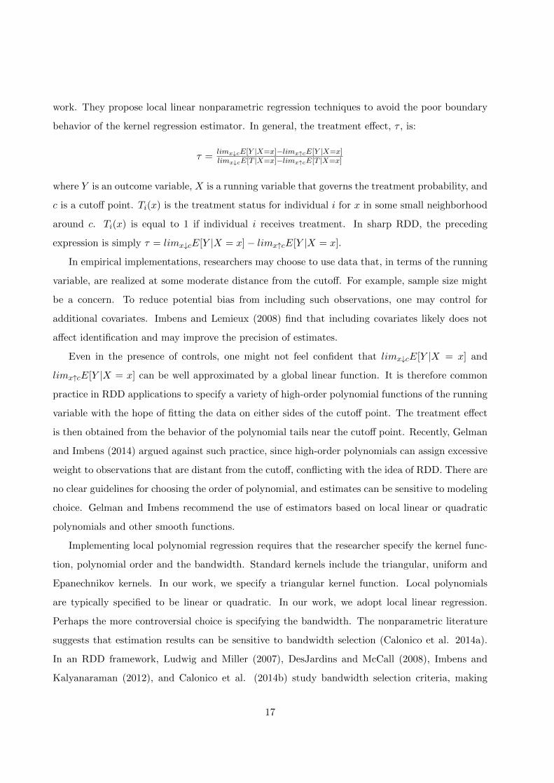
work. They propose local linear nonparametric regression techniques to avoid the poor boundary

behavior of the kernel regression estimator. In general, the treatment effect, τ , is:

τ =limx↓cE[Y |X=x]−limx↑cE[Y |X=x]limx↓cE[T |X=x]−limx↑cE[T |X=x]

where Y is an outcome variable, X is a running variable that governs the treatment probability, and

c is a cutoff point. Ti(x) is the treatment status for individual i for x in some small neighborhood

around c. Ti(x) is equal to 1 if individual i receives treatment. In sharp RDD, the preceding

expression is simply τ = limx↓cE[Y |X = x]− limx↑cE[Y |X = x].

In empirical implementations, researchers may choose to use data that, in terms of the running

variable, are realized at some moderate distance from the cutoff. For example, sample size might

be a concern. To reduce potential bias from including such observations, one may control for

additional covariates. Imbens and Lemieux (2008) find that including covariates likely does not

affect identification and may improve the precision of estimates.

Even in the presence of controls, one might not feel confident that limx↓cE[Y |X = x] and

limx↑cE[Y |X = x] can be well approximated by a global linear function. It is therefore common

practice in RDD applications to specify a variety of high-order polynomial functions of the running

variable with the hope of fitting the data on either sides of the cutoff point. The treatment effect

is then obtained from the behavior of the polynomial tails near the cutoff point. Recently, Gelman

and Imbens (2014) argued against such practice, since high-order polynomials can assign excessive

weight to observations that are distant from the cutoff, conflicting with the idea of RDD. There are

no clear guidelines for choosing the order of polynomial, and estimates can be sensitive to modeling

choice. Gelman and Imbens recommend the use of estimators based on local linear or quadratic

polynomials and other smooth functions.

Implementing local polynomial regression requires that the researcher specify the kernel func-

tion, polynomial order and the bandwidth. Standard kernels include the triangular, uniform and

Epanechnikov kernels. In our work, we specify a triangular kernel function. Local polynomials

are typically specified to be linear or quadratic. In our work, we adopt local linear regression.

Perhaps the more controversial choice is specifying the bandwidth. The nonparametric literature

suggests that estimation results can be sensitive to bandwidth selection (Calonico et al. 2014a).

In an RDD framework, Ludwig and Miller (2007), DesJardins and McCall (2008), Imbens and

Kalyanaraman (2012), and Calonico et al. (2014b) study bandwidth selection criteria, making

17

different recommendations. In our work, we adopt bandwidth tests developed by Calonico et al.

(2014b) and, alternatively, by Imbens and Kalyanaraman (2012), hereafter referred to as CCT and

IK, respectively. These criteria are asymptotically optimal under square error loss.

RDD in the evaluation of environmental and energy policy. In the environmental

economics literature, specifically with regard to the causal effect of policies on air pollution, four

recent RDD applications are worth noting. Davis (2008) and Lin Lawell et al. (2016) examine

the effect of policies restricting driving on urban air in Mexico City and Bogota. Auffhammer and

Kellogg (2011) examine the effect of gasoline content regulation on air quality, ozone in particular,

in the US. Chen et al., (2013) examines the effect of latitude-based heating subsidies on particle

pollution and life expectancy in China. Our setup is similar to the first three studies in that time

is the running variable, and their authors argue that the policies were implemented immediately

and achieved near universal compliance. We argue that such assumptions similarly fit our setting.

Similar to Auffhammer and Kellogg, our focus on ozone further makes RDD suitable, in that

its chemical reactivity implies that ambient air concentrations change quickly, for example, over

the diurnal cycle, or upon a step change before and after a policy comes into effect. Whereas

in both Davis’ and Auffhammer and Kellogg’s settings regulation was introduced with an aim to

curb external damage from air pollution, in our setting any effect on urban air from mandated

changes to the gasoline blend was an unintended consequence. It is this unintended consequence

of ethanol use that our study seeks to uncover. In Chen et al., the running variable is geographic

location (north versus south of the Huai river), and a rise in particle pollution was the unintended

consequence of an energy policy.

4.2 Specification

An observation in our study is an air monitoring site-hour-date triple. For example, to evaluate

the effect on ozone from changing the blend mandate, a single observation would be the ozone

monitor at Site 5 (Ibirapuera) at 3pm on February 15, 2010. Consider the regression model, to be

implemented separately by discontinuity (for brevity we omit subscript d):

yiht = αi0 + α ∗ treatt + fih(dateiht − datec) + βih ∗Wiht + εiht (1)

18

The dependent variable, yiht, is the natural logarithm of the measured pollutant mass concentration,

in the recorded units of µg/m3 or ppm, where i, h, and t index site (monitor), hour, and date,

respectively. Binary variable treatt is equal to 0 if the gasoline blend combusted on date t is E20,

and 1 if the gasoline blend is E25, indicating lower and higher ethanol fractions respectively. To

repeat from Section 3, we normalize the reporting of results to represent the treatment effect of

policy that increases the ethanol component, from E20 to E25.

The eighth-order polynomial in date, fih(dateiht − datec), is centered at the policy implemen-

tation date, datec. The polynomial trend is site and hour specific, to flexibly capture seasonal and

unobservable trends at the site-hour level over the half-year (180-day) sample. Similarly, the vector

of controls, denoted Wiht, is allowed to affect or co-vary with pollutant concentrations differentially

by site and hour pair, via the parameters βih.

Included in Wiht is a vector of day-of-week fixed effects, to account for (site-hour varying) weekly

cycles, e.g., systematic differences between, say, Tuesday 3pm and Friday 3pm, in the volume of

surrounding vehicle traffic impacting ozone levels at site 5. Day-of-week fixed effects also capture

weekend and public holiday variation in pollutant concentrations.

Other determinants of pollutant concentrations included in Wiht are meteorological conditions,

road congestion at one or more levels of proximity to the monitoring site, and the ethanol-to-

gasoline price ratio at the pump, which smoothly drives the choice of ethanol over gasoline fuel in

the subpopulation of bi-fuel vehicles. Specifically, we control for: a quadratic in log temperature

(0C, measured in the contemporaneous hour h); a quadratic in log radiation (W/m2); a quadratic

in log relative humidity (%), a quadratic in log wind speed (m/s); indicators for each of four wind

direction quadrants (whenever wind blows in excess of 0.5 m/s); precipitation (mm, from h to h−3);

and indicators for the base of an atmospheric thermal inversion layer recorded lying within 200m,

or between 200 and 500m, from the ground. We control for the quantity of road users by taking, on

top of site-hour specific day-of-week intercepts, the extension of traffic congestion across the city

recorded from 7am to 11am on date t (interacted with an indicator for t being a non-public holiday

weekday).30 The ethanol-to-gasoline price ratio enters vector Wiht as a third-order polynomial

(and we lag this by four days, as in Salvo and Geiger 2014). We selected these controls based

on the sensitivity of pollutant concentrations to their variation, for example, ozone’s sensitivity

30Given the opening on March 30, 2010 of the Greater Sao Paulo beltway, that removed trucks from specificinner city roads (He et al. 2016), we also add a dummy variable (interacted with site-hour) to indicate dates postinauguration; these may be relevant to the first two discontinuities, with cutoffs on February 4 and May 4, 2010.

19

to radiation and temperature, or the sensitivity of pollutant concentrations to wind speed. These

controls have added importance recalling that the effect on air of a 5-percent discontinuity in the

gasoline blend may not be large and we may lack precision. To emphasize, controls are flexibly

interacted with site by hour fixed effects.31 Appendix Figures A.1 to A.4 summarize variation in

meteorology and road congestion around each discontinuity.

The treatment effect is estimated in two steps. First, using ordinary least squares (OLS) we

estimate a restricted version of equation (1), that excludes treatt (but includes the site-hour spe-

cific eighth-order polynomials in date),32 generating fitted residuals of ln(pollutant concentration).

Intuitively, this demeans the data and partials out the effect of other factors. Second, we implement

local linear regression using the fitted residuals to estimate the treatment effect.

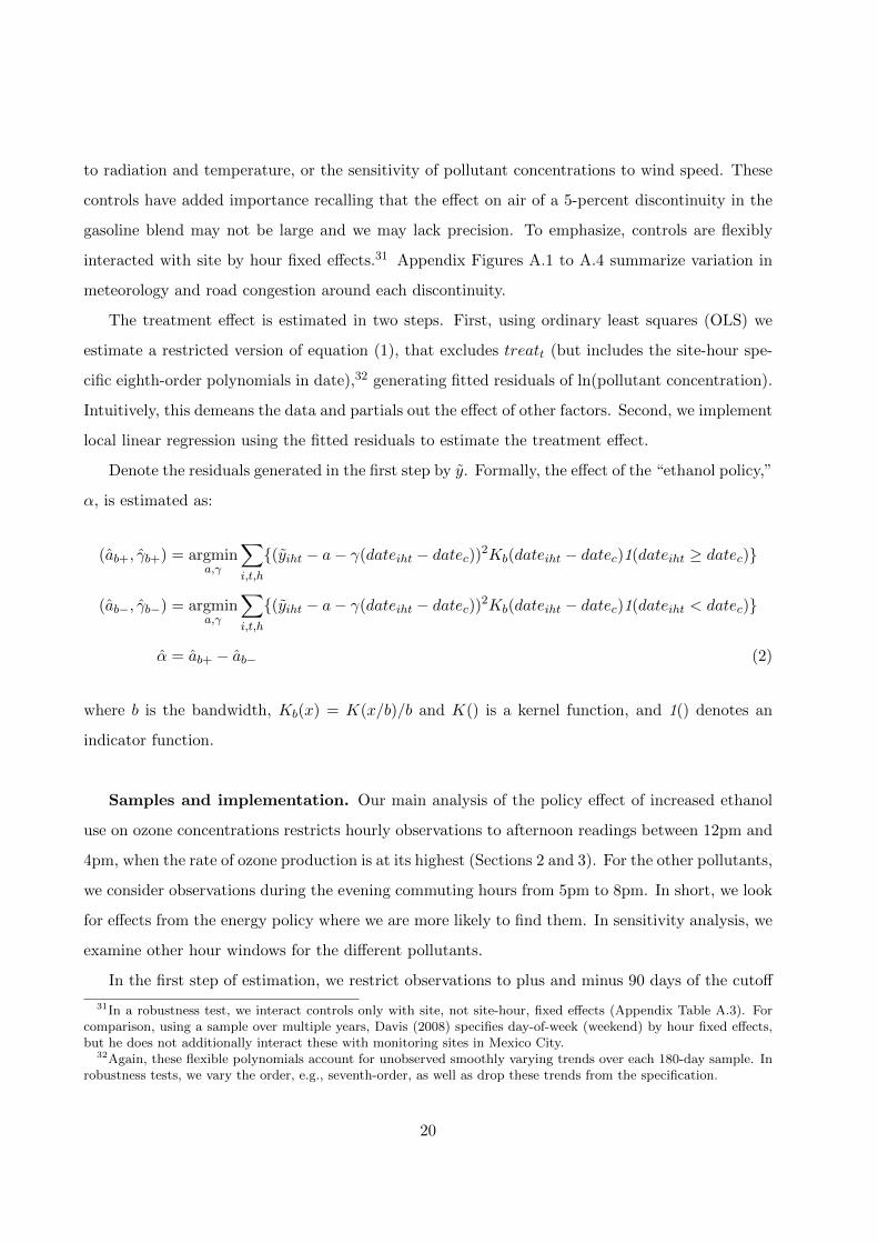
Denote the residuals generated in the first step by y. Formally, the effect of the “ethanol policy,”

α, is estimated as:

(ab+, γb+) = argmina,γ

∑i,t,h

{(yiht − a− γ(dateiht − datec))2Kb(dateiht − datec)1(dateiht ≥ datec)}

(ab−, γb−) = argmina,γ

∑i,t,h

{(yiht − a− γ(dateiht − datec))2Kb(dateiht − datec)1(dateiht < datec)}

α = ab+ − ab− (2)

where b is the bandwidth, Kb(x) = K(x/b)/b and K() is a kernel function, and 1() denotes an

indicator function.

Samples and implementation. Our main analysis of the policy effect of increased ethanol

use on ozone concentrations restricts hourly observations to afternoon readings between 12pm and

4pm, when the rate of ozone production is at its highest (Sections 2 and 3). For the other pollutants,

we consider observations during the evening commuting hours from 5pm to 8pm. In short, we look

for effects from the energy policy where we are more likely to find them. In sensitivity analysis, we

examine other hour windows for the different pollutants.

In the first step of estimation, we restrict observations to plus and minus 90 days of the cutoff

31In a robustness test, we interact controls only with site, not site-hour, fixed effects (Appendix Table A.3). Forcomparison, using a sample over multiple years, Davis (2008) specifies day-of-week (weekend) by hour fixed effects,but he does not additionally interact these with monitoring sites in Mexico City.

32Again, these flexible polynomials account for unobserved smoothly varying trends over each 180-day sample. Inrobustness tests, we vary the order, e.g., seventh-order, as well as drop these trends from the specification.

20

point (for the given discontinuity), namely three days after the mandated deadline for distributor

shipments, to allow fuel stations and consumers to adjust, as explained.33 In the second step, we

use CCT’s bandwidth selection criterion to determine the number of days before and after the

discontinuity. The tested bandwidth turns out to be about 30 days, ensuring that the 90 days we

consider in the first step suffices for the second step. Of note, the first and second discontinuities

occurred three months apart. As we examine each discontinuity one by one, we do not vary the

180-day window, with the objective of making our estimates comparable across discontinuities.

5 Results

As discussed in Section 3, we face the empirical challenge that, although gasoline fuel accounted

for the majority share of Sao Paulo’s 6 million cars and 1 million motorcycles during each of the

four discontinuities, changes to the composition of gasoline were not large. Also, ozone’s reactivity

and sensitivity to the immediate surroundings implies that concentrations can be quite variable for

unobserved, idiosyncratic reasons. This is an empirical challenge that Auffhammer and Kellogg

(2011) likely also faced. In our setting, this variability can immediately be seen from the scatter

in Figure 4 showing demeaned log afternoon ozone concentrations at the level of the data—a site-

hour-date triple—following the first step of the local linear regression estimation procedure (Section

4). The dots indicate log concentration residuals, y, with all covariates accounted for, including

meteorology and the eight-order polynomial trend over the whole 180-day period, flexibly by site-

hour. To emphasize, we estimate models separately by discontinuity throughout the analysis, and

“pool” across discontinuities only in a robustness test. The fitted lines on either side of each

discontinuity are only for illustration, as here they are based on a fixed bandwidth of 30 days

rather than the bandwidth tests reported below.

Before presenting results for our preferred local linear regression specification, Table 3 presents

estimates for regression model (1), estimated from the 180-day sample in a single step by OLS

with treatt included. The estimated effect on ambient ozone concentrations from an increase in

the ethanol content in gasoline is positive and significant at least at the 5% level across all four

discontinuities. The average point estimate and standard error across the four discontinuities is

33See Table 1. As a robustness check, we allow the mandated ethanol shift to phase in over several days, ratherthan abruptly. As explained, a fuzzy design would require that we observe the exact composition of downstream fuelinventories—the “compliance rate”—over these few days.

21

0.125 and 0.042 log points, respectively. (Standard errors shown in Table 3 are one-way clustered

at the site-date level.) Estimates of the increase in afternoon ozone levels—a 0.11 to 0.16 increase

in log points—caused by a 5 percentage point increase in the ethanol fraction appear quite large

(see below). Given concerns about the extent to which high-order polynomials can single-handedly

account for unobserved confounding factors, such as seasonality, as we move away from the cutoff,

we follow the advice of Gelman and Imbens (2014) and turn to local linear regression.

Consider again demeaned log ozone concentrations, demeaned separately by 180-day sample, at

the site-hour-date level, yiht. To account for correlation across hourly readings within date and site

(i.e., to “cluster” our inference at the site-date level), we then take the mean of the demeaned log

concentrations across hours within site-date. It is on these residual log concentrations at the site-

date level that we implement local linear regression. (We later check robustness to implementing

local linear regression directly on yiht.) Table 4, panel A presents local linear regression estimates

for the effect on mean afternoon ozone concentrations from raising the ethanol content in gasoline

fuel, under alternative bandwidths according to either the CCT or the IK criteria (Section 4).

Selected bandwidths range between 22 and 35 days and turn out to be similar across the two

criteria, for example, 22 (CCT) and 24 (IK) days on either side of the discontinuity # 3 cutoff.

Importantly, a 30-day or so bandwidth coupled with 12 sites (with sites added in 2012) implies

that the number of observations is not large—between 500 and 1,000.

Across all four discontinuities and both bandwidth selection criteria, the local regression’s es-

timated effect of ethanol on mean afternoon ozone levels is positive and somewhat lower than

direct estimates of (1) using the whole 180-day period (Table 3). Point estimates range from 0.041

(discontinuity # 4, IK) to 0.126 (discontinuity # 3, CCT), and average 0.090 log points across

discontinuities and bandwidth criteria (with an average standard error of 0.035 log points). Point

estimates under the IK criterion average 0.083 compared with 0.097 log points under CCT. These

estimated magnitudes, based on a 5 percent ethanol increase in fuel content among 70% of light

vehicles, that tended to be burning blended gasoline at the cutoff dates (Table 1), are comparable

to—if slightly higher than—point estimates reported by Salvo and Geiger (2014, Figure 4) for a

shift from E25 to E100 among 60% of bi-fuel vehicles (bi-fuel vehicles accounting for 50% of VMT

by passenger cars).

Robustness. In Table 4, panel B we alternatively take the maximum of each afternoon’s (log)

22

ozone concentrations as the dependent variable, with the resulting data at the site-date level, and

repeat the estimation routine, namely demeaning the dependent variable using a 180-day sample

followed by implementing local linear regression on a sample of bandwidth tested according to

each of the two criteria. The estimated effect of ethanol on maximum ozone levels is again positive

across all four discontinuities and both bandwidth criteria, averaging 0.081 log points.

Figure 5 shows that the estimated positive effect of ethanol on mean afternoon ozone concen-

trations, reported in Table 4A is not overly sensitive to varying the bandwidth of days around the

cutoff point. 95% confidence intervals are quite stable and remain above (or almost above) zero as

we decrease or increase the bandwidth starting at the level selected by either the CCT or the IK

criteria. Perhaps unsurprisingly, estimates can become rather less stable, with confidence bands

widening and shifting, as we reduce the bandwidth by 10 days. Estimates are somewhat more

precise as we increase the bandwidth, though this comes at the potential expense of introducing

omitted variable bias.

Figure 6 tests robustness to the demeaning of the data (at varying bandwidths). Solid lines

indicate point estimates for the treatment effect following the procedure described above (demean

the dependent variable at the observed level of the data, a site-hour-date triple, and take the mean

of the demeaned values across hours within site-date). Dashed lines indicate point estimates under

an alternative procedure, whereby we implement local linear regression directly on site-hour-date

level demeaned values, rather than on site-date level means of these values.34

Our findings are further robust to pooling the demeaned data (that goes into the second step)

across the four discontinuities, while still demeaning separately by 180-day sample in the first step

to flexibly allow for, say, seasonal variation: Table 5 reports an estimated effect of 0.081 to 0.083

log points.

Table 6 reports robustness to hour-of-the-day—mean over morning hours from 7am to 11am,

or the maximum 8-hour average (e.g., Lin et al. 2001)—and to functional form—ozone, not log

ozone, concentration. In panel D, and pooling ozone residuals across the four 180-day samples, the

effect of raising the ethanol fraction on the daily maximum 8-hour ozone average is 4.8 µg/m3 (s.e.

1.2 µg/m3), or 8.0% of the sample mean of daily maximum 8-hour averages, of 59.9 µg/m3.

We also implement local linear regression separately by ozone monitoring site (and discontinu-

34Dotted lines in the figure indicate point estimates for the treatment effect under yet another procedure, wherebywe first take means of the data across the afternoon hours from 12pm to 4pm, and only then proceed to demean thesite-date varying mean afternoon log ozone concentrations.

23

ity). Each panel of Figure 7 plots the distribution of 53 (12 + 12 + 12 + 17) point estimates across

sites and discontinuities. Most density lies on the positive domain, with medians of 0.084 and 0.063

log points, respectively under the CCT and IK criteria (a median of 0.072 log points overall).

Finally, Appendix Table A.1 reports robustness to varying the order of the polynomial trends

specified over each 180-day first-step sample. Appendix Table A.2 reports bootstrap standard

errors, in which a bootstrap sample is a sample of site-date pairs, to account for sampling variation

in the first step. As an alternative to clustering at the site-date level, we alternatively bootstrap the

sample at the site-week level. In the second step, we alternatively fix the bandwidth selected from

the original sample, or select the bandwidth according to each bootstrap sample. Appendix Table

A.4 considers specifications in which we allow the mandated ethanol shift to phase in over a few

days, rather than abruptly. In the sensitivity analysis shown in Appendix Table A.5, we control

for meteorology as quadratic functions of the levels (not logarithms) of temperature, radiation,

humidity and wind speed, or via bins (temperature every 10C, radiation every 150 W/m2).

Other robustness tests—not shown for brevity—include widening the first-step sample beyond

180 days, or specifying a uniform rather than triangular kernel. We add variables (sunshine hours)

or high-order terms (quartic rather than quadratic) in the vector of meteorological controls. We

include, as separate controls, monthly gasoline and ethanol fuel shipments reported by distributors

to the state market—while too aggregate in time and space, these are the quantity data that are

available (Figure 1(c)). Our findings are also robust to specifying the cutoff point at four days

(rather than our preferred three) from the mandated distributor deadline.

Ethanol and PM2.5, CO and NOx. Table 7 provides local linear regression estimates for

the effect on ambient PM2.5, CO and NOx levels from raising gasoline fuel’s ethanol content—see

panels A, B and C, respectively. We follow exactly the same procedure as we implemented when

evaluating the policy effect on ozone (Table 4A), recalling that now we consider evening commuting

hours of peak traffic congestion, between 5pm and 8pm (Table 2), rather than afternoon hours of

peak ozone formation.

Averaging across discontinuities and bandwidth criteria, point estimates in log points are -0.034

for PM2.5, -0.019 for CO and -0.059 for NOx. Estimates tend to be smaller in magnitude than in

the case for ozone, and they tend not to be significantly different than zero. Estimates on NOx are

less precise than in the case for ozone, i.e., standard errors across discontinuities and bandwidth

24

criteria average 0.057 and 0.035 log points for NOx and ozone, respectively, with inference in both

cases relying on a similar number of monitors in the metropolis. Pooling residuals across all 180-day

samples in a single (second-step) regression, point estimates for NOx are a statistically negative

-0.077 log points under the CCT criterion. Salvo and Geiger (2014) found NO levels to fall with

increased ethanol penetration and their estimates for NO were less precise compared to ozone.

PM2.5 levels do not appear to fall with higher ethanol penetration, or at least we are unable

to detect a fall, as our inference relies on a low number of monitors (one and three for the last

two discontinuities). Estimates for other hours (morning commuting hours, 7am to 11am) and

separate NO and NO2 components similarly tend to be smaller in magnitude and less precise than

for ozone (not shown for brevity). Unfortunately, atmospheric levels of VOCs such as formaldehyde,

acetaldehyde and ethanol are not routinely monitored (Nogueira et al. 2014).

6 Conclusion

This paper exploits four sharp discontinuities in the ethanol component of blended gasoline sold

across Brazil to assess the effect on air quality in the Sao Paulo metropolis from raising the fraction

of ethanol in the gasoline-ethanol light transportation fuel mix. These ethanol policy changes, each

amounting to 5 percentage points by volume, were spaced at least three months apart and were

mandated by the central government not as a response to urban air pollution, but to intervene in

the quantity and price outcomes of the sugar industry (sugar and ethanol products to domestic

and export markets), or simply to reverse previous changes. We test that the blend discontinuities

did not lead to price discontinuities, and argue that composition changes were not salient to fuel

consumers (and, if they were, likely responses would help us detect the effect of increased ethanol

on urban air outcomes). Using available data, we check that on each occasion, blended gasoline

accounted for the majority of distance traveled by the fleet of passenger cars and motorcycles in

the state of Sao Paulo. Our focus is on ozone, which often exceeds the local 8-hour air quality

standard (71 ppb, comparable to the US EPA’s 70 ppb), is the one regulated pollutant whose levels

have not trended downward in the past decade, and whose relevance is likely to grow in a warming

climate. We also test for effects on other monitored species, PM2.5 in particular.

Across the four discontinuities, which we examine separately to allow for unobserved hetero-

geneity, we find that ozone levels rose by about 8 percent as the gasoline blend shifted from E20 to

25

E25, i.e., toward a higher ethanol fraction. Such observational evidence (1) is consistent (in sign

and magnitude) with the results of a recent empirical study that exploited consumers smoothly

substituting between E20/E25 gasoline and E100 ethanol, (2) is theoretically consistent with ozone

formation over urban Sao Paulo being VOC-limited, (3) enables the credible inference of the health

damage of ozone that, at 70 ppb, is hotly debated, and (4) is opposite in sign to the predictions of

an atmospheric modeling study for Sao Paulo, based on emissions inventories and modeled chemical

and physical reactions, that suggested sizable ozone abatement from a hypothetical shift to ethanol

by the light-vehicle fleet. In contrast to ozone, point estimates of changes to PM2.5 are small in

magnitude but confidence intervals are wide.

Since the ethanol-blended gasoline policy changes were common across the country, future

research can examine their effect on ozone pollution at locations outside of the Sao Paulo metropolis.

For example, over the period 2010 to 2013, ozone monitors were in place in about 15 cities in the

state of Sao Paulo, with distances ranging from 100 to 600 km from the metropolis, and populations

varying by almost an order of magnitude (0.1 to 0.6 million). To the extent that atmospheric

ozone production regimes differ by locality (and possibly season)—to be proxied, for example, by

weekend-weekday ozone concentration ratios, population size, and/or prevailing winds from the

Sao Paulo megacity transporting NOx-rich air parcels over varying distances—one may examine

heterogeneous effects of increased ethanol penetration on ambient ozone levels.35

In a country where sugarcane ethanol is commonly perceived by consumers and described by

policymakers as a policy to abate gasoline emissions and improve air quality (e.g., Salvo and Huse

2013, CBN Noticias 2010, Angelo 2012), we hope that our research will better inform the public

discourse. Our research is also supportive of recent calls for a review of current vehicle emissions

standards that allow the deduction of the mass of unburned ethanol, itself a reactive VOC, emitted

from the tailpipe. We caution that our findings do not speak to other potential life-cycle benefits

and costs of substituting ethanol (current or future generation) for gasoline, nor do they make

assumptions on how on-board emissions control technologies might evolve. Moreover, we caution

that our analysis applies only to pollutants that are currently routinely monitored by Sao Paulo’s

(and other) environmental authorities, thus ignoring possible effects, in particular, on particle levels

in the submicron (< 1µm or PM1) and nanometer (< 0.1µm or PM0.1) size ranges.

Beyond Sao Paulo, our findings may be relevant to urban areas with a VOC-limited atmosphere—

35Preliminary analysis suggests that this research direction is promising. We are grateful to a Reviewer for sug-gesting it.

26

which the literature suggests is common to many densely populated cities in the US, Europe and

Asia—and countries that are planning to increase ethanol blending requirements, whether to meet

local regulation or international agreements, such as the RFS in the US and the INDCs pledged

during COP21 in Paris.

27

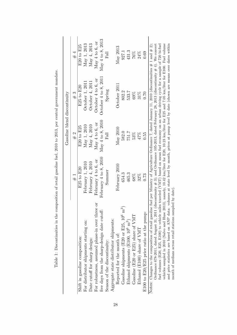
Tab

le1:

Dis

conti

nu

itie

sin

the

com

posi

tion

of

reta

ilgaso

lin

efu

el,

2010

to2013,

per

centr

al

gov

ern

men

tm

an

date

.

Gas

olin

eb

len

dd

isco

nti

nu

ity

#1

#2

#3

#4

Sh

ift

inga

soli

ne

com

pos

itio

n:

E25

toE

20E

20to

E25

E25

toE

20E

20to

E25

For

dis

trib

uto

rsh

ipm

ents

start

ing

on

:F

ebru

ary

1,20

10M

ay1,

2010

Oct

ober

1,20

11M

ay1,

2013

Date

cuto

fffo

rsh

arp

des

ign

:F

ebru

ary

4,20

10M

ay4,

2010

Oct

ober

4,20

11M

ay4,

2013

For

rob

ust

nes

s,ass

um

edp

hase

-in

over

thre

eor

Feb

ruar

y4

to6,

orM

ay4

to6,

orO

ctob

er4

to6,

orM

ay4

to6,

orfi

veday

sfr

omth

esh

arp

-des

ign

date

cuto

ff:

Feb

ruar

y4

to8,

2010

May

4to

8,20

10O

ctob

er4

to8,

2011

May

4to

8,20

13S

easo

nof

the

dis

conti

nu

ity:

Su

mm

erF

all

Sp

rin

gF

all

Agg

regate

state

dis

trib

uto

rsh

ipm

ents

:R

eport

edfo

rth

em

onth

of:

Feb

ruar

y20

10M

ay20

10O

ctob

er20

11M

ay20

13G

asoli

ne

ship

men

ts(E

20or

E25,

106

m3)

654.

358

2.0

802.

292

7.1

Eth

an

ol

ship

men

ts(E

100,

106

m3)

465.

375

1.7

533.

743

1.3

Gaso

lin

e(E

20or

E25

)sh

are

of

VM

T68

%53

%69

%76

%E

than

ol

(E10

0)

share

ofV

MT

32%

47%

31%

24%

E100

toE

20/E

25p

rice

rati

oat

the

pu

mp

:0.

730.

550.

700.

69

Note

s:C

hanges

toth

eco

mp

osi

tion

of

reta

ilgaso

line

fuel

per

Min

istr

yof

Agri

cult

ure

Ord

inance

7,

date

dJanuary

11,

2010

(dis

conti

nuit

ies

#1

and

#2);

Ord

inance

678-2

011,

date

dA

ugust

31,

2011

(dis

conti

nuit

y#

3);

and

Ord

inance

105-2

013,

date

dF

ebru

ary

28,

2013

(dis

conti

nuit

y#

4).

We

conver

tfu

elvolu

mes

(E20,

E25,

E100)

toveh

icle

miles

trav

eled

(VM

T)

base

don

mea

nfu

elec

onom

yon

an

urb

an

dri

vin

gcy

cle

for

asa

mple

of

720

bi-

fuel

veh

icle

ssa

mple

din

2010

(Salv

oand

Huse

2013),

nam

ely,

10.4

2km

/lite

rfo

rE

20,

10.2

3km

/lite

rfo

rE

25

and

7.0

5km

/lite

rfo

rE

100.

Fuel

volu

me

and

pri

cest

ati

stic

sare

base

don

AN

Pdata

:volu

mes

at

state

level

by

month

,pri

ces

at

pum

ple

vel

by

date

(show

nare

mea

ns

over

date

sw

ithin

month

of

med

ians

acr

oss

reta

ilst

ati

ons

sam

ple

dby

date

).

28

Tab

le2:

Des

crip

tive

stati

stic

sfo

rth

efo

ur

180-d

aysa

mp

les

poole

dto

get

her

.

(1)

(2)

(3)

(4)

(5)

Var

iab

les

NM

ean

Std

.Dev

.M

in.

Max.

O3

con

centr

atio

n(µ

g/m

3,

hou

rly

read

ings

7am

to11

am

)43,9

03

22.6

820.9

60

179

O3

con

centr

atio

n(µ

g/m

3,

hou

rly

read

ings

12p

mto

4p

m)

44,2

28

66.2

936.6

80

353

E25

,n

otE

20,

gaso

lin

e(y

es=

1)44,2

28

0.5

00.5

00

1P

M2.

5co

nce

ntr

atio

n(µ

g/m

3,

hou

rly

readin

gs7a

mto

11am

)3,3

07

19.9

613.5

00

97

PM

2.5

con

centr

atio

n(µ

g/m

3,

hou

rly

readin

gs5p

mto

8p

m)

2,6

07

18.6

011.2

70

86

CO

con

centr

atio

n(p

pm

,h

ourl

yre

adin

gs7a

mto

11am

)41,8

33

1.0

60.7

10

7C

Oco

nce

ntr

atio

n(p

pm

,h

ourl

yre

adin

gs5p

mto

8pm

)33,9

21

1.0

10.7

10

10.2

2N

Ox

con

centr

atio

n(p

pb

,h

ourl

yre

adin

gs7a

mto

11am

)39,2

26

74.4

770.8

40

701

NO

xco

nce

ntr

atio

n(p

pb

,h

ourl

yre

adin

gs5p

mto

8pm

)31,8

43

52.0

654.6

80

588

Tem

per

atu

re(0

C,

hou

rly

read

ings

7am

to11

am)

3,5

99

19.7

24.1

96.1

532.3

7T

emp

erat

ure

(0C

,h

ourl

yre

adin

gs12

pm

to4p

m)

3,6

00

24.9

74.7

77.6

935.9

7R

adia

tion

(W/m

2,

hou

rly

read

ings

7am

to11

am)

3,5

99

240.6

6219.7

20

893

Rad

iati

on(W

/m2,

hou

rly

read

ings

12p

mto

4pm

)3,6

00

513.6

6241.2

213.2

01128.5

0R

elat

ive

hu

mid

ity

(%,

hou

rly

read

ings

7am

to11

am)

3,5

99

80.3

513.9

226

97.9

8R

elat

ive

hu

mid

ity

(%,

hou

rly

read

ings

12p

mto

4pm

)3,6

00

58.5

617.9

613.5

098

Win

dsp

eed

(m/s

,h

ourl

yre

adin

gs7a

mto

11am

)3,5

99

1.3

70.6

70.0

23.9

9W

ind

spee

d(m

/s,

hou

rly

read

ings

12p

mto

4pm

)3,6

00

2.0

40.6

70.2

85.2

0P

reci

pit

atio

n(m

m/h

,h

ourl

yre

adin

gs7a

mto

11am

)3,5

92

0.1

20.7

90

16.8

0P

reci

pit

atio

n(m

m/h

,h

ourl

yre

adin

gs12

pm

to4p

m)

3,5

97

0.2

21.6

50

43.8

0W

ind

blo

ws

from

N-E

(yes

=1,

hou

rly

read

ings

7am

to11am

)13,3

85

0.2

80.4

50

1W

ind

blo

ws

from

N-W

(yes

=1,

hou

rly

read

ings

7am

to11am

)13,3

85

0.2

20.4

10

1W

ind

blo

ws

from

S-W

(yes

=1,

hou

rly

read

ings

7am

to11am

)13,3

85

0.0

70.2

60

1W

ind

blo

ws

from

S-E

(yes

=1,

hou

rly

read

ings

7am

to11am

)13,3

85

0.3

30.4

70

1W

ind

blo

ws

from

N-E

(yes

=1,

hou

rly

read

ings

12pm

to4p

m)

13,3

79

0.1

40.3

40

1W

ind

blo

ws

from

N-W

(yes

=1,

hou

rly

read

ings

12p

mto

4p

m)

13,3

79

0.4

10.4

90

1W

ind

blo

ws

from

S-W

(yes

=1,

hou

rly

read

ings

12pm

to4p

m)

13,3

79

0.1

10.3

10

1W

ind

blo

ws

from

S-E

(yes

=1,

hou

rly

read

ings

12p

mto

4p

m)

13,3

79

0.3

40.4

70

1T

her

mal

inve

rsio

nat

9am

,b

ase

0-20

0m(y

es=

1)718

0.0

90.2

90

1T

her

mal

inve

rsio

nat

9am

,b

ase

200-

500m

(yes

=1)

718

0.2

70.4

40

1T

her

mal

inve

rsio

nat

9pm

,b

ase

0-20

0m(y

es=

1)717

0.2

50.4

30

1T

her

mal

inve

rsio

nat

9pm

,b

ase

200-

500m

(yes

=1)

717

0.1

20.3

30

1R

oad

con

gest

ion

(km

,ci

tyw

ide,

hou

rly

read

ings

7am

to11am

)3,6

00

35.3

233.6

20

156.3

8R

oad

con

gest

ion

(km

,ci

tyw

ide,

hou

rly

read

ings

5pm

to8p

m)

2,8

80

57.3

350.0

50

277.2

0P

er-l

iter

eth

anol

-to-

gaso

lin

ep

rice

rati

o720

66.3

55.8

652.6

374.1

3

Not

es:

The

sam

ple

consi

sts

of

90

day

son

eith

ersi

de

of

the

cuto

ffdate

for

each

of

the

four

dis

conti

nuit

ies

des

crib

edin

Table

1.

For

polluta

nt

conce

ntr

ati

ons,

an

obse

rvati

on

isa

date

-hour

by

site

(wit

hin

the

indic

ate

dhour

win

dow

).F

or

the

E25

gaso

line

indic

ato

r,an

obse

rvati

on

isa

date

-hour

by

ozo

ne

site

(wit

hin

the

12pm

to4pm

win

dow

)fo

rw

hic

hozo

ne

conce

ntr

ati

ons

wer

ere

cord

ed,

wit

hth

epurp

ose

of

dem

onst

rati

ng

that

ozo

ne

mea

sure

men

tsare

sim

ilarl

yav

ailable

on

eith

ersi

de

of

the

cuto

ffdate

s.F

or

met

eoro

logy

and

city

wid

ero

ad

conges

tion,

an

obse

rvati

on

isa

date

-hour

(we

aver

age

acr

oss

wea

ther

stati

ons)

,ex

cept

win

ddir

ecti

on,

wher

ean

obse

rvati

on

isa

date

-hour

by

site

(ther

eare

up

tofive

site

sm

easu

ring

win

ddir

ecti

on).

Win

ddir

ecti

on

isin

tera

cted

wit

ha

dum

my

vari

able

indic

ati

ng

that

win

dis

blo

win

gat

asp

eed

inex

cess

of

0.5

m/s.

For

the

fuel

pri

cera

tio,

an

obse

rvati

on

isa

date

.See

the

text

for

sourc

es.

29

Table 3: OLS regression for Ozone using the 180-day sample, with an eighth-order polynomial trend overthe whole period (afternoon hours).

Gasoline blend discontinuity

# 1 # 2 # 3 # 4Summer 2010 Fall 2010 Spring 2011 Fall 2013

Dependent variable: Log ozone concentration, by site-hour-dateE25, not E20, gasoline (yes=1) 0.110** 0.157*** 0.117*** 0.116***

i.e., higher ethanol content (0.043) (0.050) (0.036) (0.039)Control variables (all effects by site-hour)

Site by hour fixed effects interacted with:Eighth-order polynomial time trend Yes Yes Yes YesDay-of-week fixed effects Yes Yes Yes YesMeteorological conditions Yes Yes Yes YesThermal inversion indicators Yes Yes Yes YesRoad traffic congestion Yes Yes Yes YesEthanol-to-gasoline price ratio (cubic) Yes Yes Yes Yes

R2 82% 86% 84% 83%Number of observations 9,852 10,056 10,122 13,487Number of regressors 2,161 2,161 2,101 2,976Number of sites 12 12 12 17

Notes: *** p<0.01, ** p<0.05, * p<0.1. An observation is a site-hour-date triple. The sample includes all hoursbetween 12pm and 4pm on all dates that are plus and minus 90 days of the cutoff point (February 4, 2010for # 1; May 4, 2010 for # 2; October 4, 2011 for # 3; May 4, 2013 for # 4) for all monitoring sites that areactive in the Sao Paulo metropolitan area (by active we require at least 70% of a maximum of 180× 5 = 900hourly measurements to be available in a 180-day period). The dependent variable is the logarithm ofhourly ozone concentration (µg/m3). Meteorological conditions include quadratics in contemporaneous logtemperature, log radiation, log humidity and log wind speed; indicators for contemporaneous wind blowingin from each of four wind direction quadrants; mean precipitation in the contemporaneous hour to threehours earlier. Other covariates include indicators for the base of an atmospheric thermal inversion layer lyingwithin 200m, or between 200 and 500m, from the ground, according to the 9am or 9pm reading, whicheveris closest to the given hour; the log of citywide extension of traffic congestion from 7am to 11am interactedwith an indicator for the date being a weekday and non-public holiday; a cubic in the ethanol-to-gasolineprice ratio lagged by 4 days. All controls enter the specification interacted with site by hour fixed effects.OLS estimates for four separate regressions. Standard errors, in parentheses, are clustered by site-date pair.

30

Table 4: Local linear regression for Mean Ozone and Maximum Ozone (afternoon hours).

Gasoline blend discontinuity

# 1 # 2 # 3 # 4Summer 2010 Fall 2010 Spring 2011 Fall 2013

A: Dependent variable: Mean (of demeaned) log ozone concentration, by site-dateCCT bandwidth criterionE25, not E20, gasoline (yes=1) 0.070** 0.112** 0.126*** 0.078***

i.e., higher ethanol content (0.032) (0.045) (0.036) (0.029)Bandwidth 30 25 22 28Number of observations 642 550 482 883IK bandwidth criterionE25, not E20, gasoline (yes=1) 0.066** 0.105*** 0.118*** 0.041

i.e., higher ethanol content (0.032) (0.037) (0.035) (0.032)Bandwidth 31 35 24 23Number of observations 663 778 526 726Number of sites 12 12 12 17

B: Dependent variable: Demeaned maximum of log ozone concentration, by site-dateCCT bandwidth criterionE25, not E20, gasoline (yes=1) 0.102*** 0.094** 0.054 0.080**

i.e., higher ethanol content (0.033) (0.046) (0.039) (0.036)Bandwidth 27 27 26 29Number of observations 568 594 619 1,001IK bandwidth criterionE25, not E20, gasoline (yes=1) 0.091*** 0.096** 0.054 0.079**

i.e., higher ethanol content (0.032) (0.043) (0.039) (0.036)Bandwidth 32 31 26 28Number of observations 679 685 619 965Number of sites 12 12 12 17

Notes: *** p<0.01, ** p<0.05, * p<0.1. An observation in the second step is a site-date pair within thebandwidth (in days from the cutoff point) specified by either the CCT or IK selection criterion,for all monitoring sites that are active in the Sao Paulo metropolitan area. See the text for thefirst-step procedure: to demean hourly log pollutant concentrations (12pm to 4pm) using each180-day sample, and to collapse residual concentrations to the site-date level taking the mean acrosshours (panel A); or to take the maximum log pollutant concentration between 12pm and 4pm, andto demean these site-date varying maximum values using each 180-day sample (panel B). See thenotes to Table 3 for site-hour (site in panel B) specific eighth-order polynomial trend, day-of-weekfixed effects, meteorology, thermal inversion, road traffic congestion and fuel price controls used todemean the data. Local linear regression estimates for 16 separate regressions. Robust standarderrors in parentheses.

31

Table 5: Local linear regression for Mean Ozone (afternoon hours): Sensitivity to pooling across the four180-day samples.

Gasoline blend discontinuity

# 1, # 2, # 3, # 4 pooled together,stacked by day plus or minus from cutoff

Dependent variable: Mean (of demeaned) log ozone concentration, by site-dateCCT bandwidth criterionE25, not E20, gasoline (yes=1) 0.081***

i.e., higher ethanol content (0.017)Bandwidth 23Number of observations 2,221IK bandwidth criterionE25, not E20, gasoline (yes=1) 0.083***

i.e., higher ethanol content (0.016)Bandwidth 27Number of observations 2,619Number of site-discontinuity pairs 12 + 12 + 12 + 17 = 53

Notes: *** p<0.01, ** p<0.05, * p<0.1. An observation in the second step is a site-date pairwithin the bandwidth (in days from the cutoff point) specified by either the CCT or IKselection criterion, for all monitoring sites that are active in the Sao Paulo metropolitanarea. The first step (demeaning hourly log ozone concentrations separately by 180-daysample and taking means across hours within site-date) follows Table 4A exactly. Locallinear regression estimates for two separate regressions. Robust standard errors inparentheses.

32

Table 6: Local linear regression for Mean Ozone: Sensitivity to hour-of-the-day and functional form.

Gasoline blend discontinuity All four

# 1 # 2 # 3 # 4 pooledSum. ’10 Fall ’10 Spr. ’11 Fall ’13 together

A: Dependent variable: Mean (of demeaned) log ozone concentration, 7am to 11amCCT E25, not E20, gasoline (yes=1) 0.121 0.187** 0.165*** 0.084 0.121***

i.e., higher ethanol content (0.118) (0.089) (0.057) (0.054) (0.040)Bandwidth 27 24 34 36 25

IK E25, not E20, gasoline (yes=1) 0.093 0.182** 0.175*** 0.043 0.121***i.e., higher ethanol content (0.107) (0.087) (0.059) (0.062) (0.038)

Bandwidth 33 25 32 29 27

B: Dep. var.: Mean (of demean.) log ozone conc., 11am to 6pm (modal 8-hour period for max.)CCT E25, not E20, gasoline (yes=1) 0.054 0.160*** 0.142*** 0.033 0.072***

i.e., higher ethanol content (0.035) (0.046) (0.039) (0.030) (0.018)Bandwidth 30 24 21 28 24

IK E25, not E20, gasoline (yes=1) 0.051 0.149*** 0.094*** 0.026 0.074***i.e., higher ethanol content (0.034) (0.040) (0.033) (0.031) (0.017)

Bandwidth 33 32 32 27 27

C: Dep. var.: Mean (of demeaned) log ozone concentration, maximum 8-hour average (realized)CCT E25, not E20, gasoline (yes=1) 0.080* 0.156*** 0.060* 0.066** 0.072***

i.e., higher ethanol content (0.042) (0.047) (0.035) (0.032) (0.019)Bandwidth 31 24 25 32 26

IK E25, not E20, gasoline (yes=1) 0.072* 0.095*** 0.068** 0.029 0.072***i.e., higher ethanol content (0.041) (0.031) (0.032) (0.037) (0.019)

Bandwidth 34 56 32 25 26

D: Dep. var.: Mean (of demeaned) ozone concentration, maximum 8-hour average (realized)CCT E25, not E20, gasoline (yes=1) 10.99*** 2.06 6.52** 3.76* 4.74***

i.e., higher ethanol content (3.04) (2.18) (2.69) (2.03) (1.23)Bandwidth 23 35 34 26 27

IK E25, not E20, gasoline (yes=1) 11.07*** 1.80 6.37** 3.49* 4.79***i.e., higher ethanol content (2.67) (1.97) (3.21) (1.90) (1.20)

Bandwidth 28 41 24 29 28Mean value dep.var. (max 8-h avg., µg/m3) 62.07 55.70 72.28 52.24 59.85

No. of sites (site-discontinuity pairs) 12 12 12 17 53

Notes: *** p<0.01, ** p<0.05, * p<0.1. All notes to Tables 4 and 5 (respectively, second-step regressions areseparate by discontinuity or pooled across discontinuities) apply here. Instead of afternoon hours (12pmto 4pm), panels A and B consider morning hours (7am to 11am) and the modal (most common) 8-hourperiod for daily maximum 8-hour averages (11am to 6pm), respectively. Panel C considers the realized8-hour period, by site-date in each 180-sample, of daily maximum 8-hour averages. Since this realized8-hour period varies from day to day (e.g., 10am to 5pm versus 11am to 6pm), we interact first-stepcontrols only with site fixed effects, as in Table A.3, with the exception of day-of-week which we interactwith site-hour fixed effects. Panel D follows the third panel but considers (the mean of demeaned)ozone concentrations rather than log ozone concentrations as in Tables 4 and 5. Local linear regressionestimates for 40 separate regressions. For brevity, we omit the number of observations (these scale withthe tested bandwidth). Robust standard errors in parentheses.

33

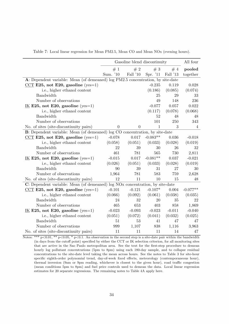
Table 7: Local linear regression for Mean PM2.5, Mean CO and Mean NOx (evening hours).

Gasoline blend discontinuity All four

# 1 # 2 # 3 # 4 pooledSum. ’10 Fall ’10 Spr. ’11 Fall ’13 together

A: Dependent variable: Mean (of demeaned) log PM2.5 concentration, by site-dateCCT E25, not E20, gasoline (yes=1) -0.235 0.119 0.028

i.e., higher ethanol content (0.186) (0.085) (0.074)Bandwidth 25 29 33Number of observations 49 148 236

IK E25, not E20, gasoline (yes=1) -0.077 0.057 0.022i.e., higher ethanol content (0.117) (0.078) (0.068)

Bandwidth 52 48 48Number of observations 101 250 343

No. of sites (site-discontinuity pairs) 0 0 1 3 4

B: Dependent variable: Mean (of demeaned) log CO concentration, by site-dateCCT E25, not E20, gasoline (yes=1) -0.078 0.017 -0.083** 0.036 -0.018

i.e., higher ethanol content (0.058) (0.051) (0.033) (0.028) (0.019)Bandwidth 22 39 30 26 32Number of observations 461 781 565 730 2,811

IK E25, not E20, gasoline (yes=1) -0.015 0.017 -0.081** 0.037 -0.021i.e., higher ethanol content (0.026) (0.051) (0.033) (0.028) (0.019)

Bandwidth 90 39 31 27 30Number of observations 1,964 781 583 759 2,628

No. of sites (site-discontinuity pairs) 12 11 10 15 48

C: Dependent variable: Mean (of demeaned) log NOx concentration, by site-dateCCT E25, not E20, gasoline (yes=1) -0.101 -0.121 -0.107* 0.004 -0.077**

i.e., higher ethanol content (0.066) (0.092) (0.061) (0.038) (0.035)Bandwidth 24 32 20 35 22Number of observations 465 653 403 858 1,869

IK E25, not E20, gasoline (yes=1) -0.023 -0.093 -0.023 -0.011 -0.040i.e., higher ethanol content (0.051) (0.072) (0.041) (0.032) (0.025)

Bandwidth 51 53 41 47 47Number of observations 999 1,107 838 1,116 3,963

No. of sites (site-discontinuity pairs) 11 11 11 14 47

Notes: *** p<0.01, ** p<0.05, * p<0.1. An observation in the second step is a site-date pair within the bandwidth(in days from the cutoff point) specified by either the CCT or IK selection criterion, for all monitoring sitesthat are active in the Sao Paulo metropolitan area. See the text for the first-step procedure to demeanhourly log pollutant concentrations (5pm to 8pm) using each 180-day sample, and to collapse residualconcentrations to the site-date level taking the mean across hours. See the notes to Table 3 for site-hourspecific eighth-order polynomial trend, day-of-week fixed effects, meteorology (contemporaneous hour),thermal inversion (9am or 9pm reading, whichever is closest to the given hour), road traffic congestion(mean conditions 5pm to 8pm) and fuel price controls used to demean the data. Local linear regressionestimates for 20 separate regressions. The remaining notes to Table 4A apply here.

34

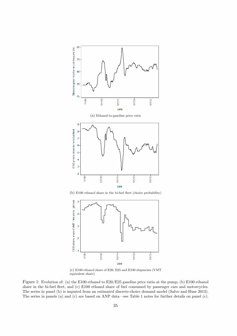
(a) Ethanol-to-gasoline price ratio

(b) E100 ethanol share in the bi-fuel fleet (choice probability)

(c) E100 ethanol share of E20, E25 and E100 shipments (VMTequivalent share)

Figure 1: Evolution of: (a) the E100 ethanol to E20/E25 gasoline price ratio at the pump, (b) E100 ethanolshare in the bi-fuel fleet, and (c) E100 ethanol share of fuel consumed by passenger cars and motorcycles.The series in panel (b) is imputed from an estimated discrete-choice demand model (Salvo and Huse 2013).The series in panels (a) and (c) are based on ANP data—see Table 1 notes for further details on panel (c).

35

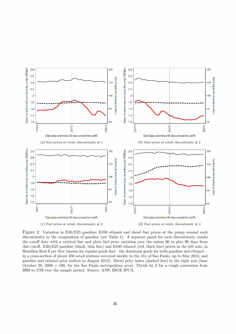
(a) Fuel prices at retail, discontinuity # 1 (b) Fuel prices at retail, discontinuity # 2

(c) Fuel prices at retail, discontinuity # 3 (d) Fuel prices at retail, discontinuity # 4

Figure 2: Variation in E20/E25 gasoline, E100 ethanol and diesel fuel prices at the pump around eachdiscontinuity in the composition of gasoline (see Table 1). A separate panel for each discontinuity marksthe cutoff date with a vertical line and plots fuel price variation over the minus 90 to plus 90 days fromthis cutoff. E20/E25 gasoline (black, thin line) and E100 ethanol (red, thick line) prices in the left axis, inBrazilian Real $ per liter (means for regular-grade fuel—the dominant grade for both gasoline and ethanol—in a cross-section of about 350 retail stations surveyed weekly in the city of Sao Paulo, up to May 2013, andgasoline and ethanol price indices to August 2013). Diesel price index (dashed line) in the right axis (baseOctober 30, 2008 = 100, for the Sao Paulo metropolitan area). Divide by 2 for a rough conversion fromBR$ to US$ over the sample period. Source: ANP, IBGE IPCA.

36

Site 5

Site 20

Site 1

Site 29

Site 7

Site 27

Site 17

Site 15

Site 6

Site 31

Site 16

Site 8

Site 3

Site 10

Site 32Site 22

Site 18

Site 2

5 km

Centerregion East

region

Northregion

Westregion

Southregion

Site 33

Site 35

Site 36

Site 37

Site 28

O3

PM2.5CONO

Legend:

Figure 3: Location of the state EPA’s air monitoring sites in the Sao Paulo metropolitan area (40 munici-palities), monitoring ozone, PM2.5, CO and NOx (NO and NO2), between 2010 and 2013, superimposed onthe grid of road corridors that is monitored by the city’s traffic authority for traffic congestion. Only regionsin the city of Sao Paulo, a subset of the metropolitan area, are shaded. Air monitoring site names are: (1)Parque Dom Pedro II, (2) Santana, (3) Mooca, (5) Ibirapuera, (6) Nossa Senhora do O, (7) Sao Caetano doSul, (8) Congonhas, (10) Cerqueira Cesar, (15) Diadema, (16) Santo Amaro, (17) Osasco, (18) Santo Andre-Capuava, (20) Taboao da Serra, (22) Maua, (27) Pinheiros, (29) Parelheiros, (31) IPEN-USP, (32) SantoAndre-Paco Municipal, (33) Itaim Paulista, (35) Guarulhos-Paco Municipal, (36) Marginal Tiete-Ponte dosRemedios, (37) Capao Redondo. Source: CETESB, CET.

37

(a) Log ozone residuals, discontinuity # 1 (b) Log ozone residuals, discontinuity # 2

(c) Log ozone residuals, discontinuity # 3 (d) Log ozone residuals, discontinuity # 4

Figure 4: Demeaned log ozone concentrations, following the first step of the local linear regression estimationprocedure, based on a 180-day sample separately by discontinuity. An observation is a site-hour-date triple,across afternoon hours (12pm to 4pm) and active ozone-monitoring sites. Only to illustrate, we plot fittedlines (with 95% confidence interval) on either side of each cutoff point fixing the bandwidth at 30 days.Since the first and third discontinuity involved a shift, over time, from E25 to E20, the horizontal axis ofpanels (a) and (c) shows observations going backward in time. For example, in panel (a), the day labeled 0is February 4, 2010, day 1 is February 3, 2010, and day -1 is February 5, 2010.

38

(a) E20 to E25 treatment effect, discontinuity # 1 (b) E20 to E25 treatment effect, discontinuity # 2

(c) E20 to E25 treatment effect, discontinuity # 3 (d) E20 to E25 treatment effect, discontinuity # 4

Figure 5: Local linear regression estimates of the E25 treatment effect on mean afternoon log ozone concen-trations. 95% confidence intervals are plotted. Sensitivity analysis to variation in the optimal bandwidth,marked by dashed vertical lines (Table 4A), according to the CCT and IK criteria.

39

(a) E20 to E25 treatment effect, discontinuity # 1 (b) E20 to E25 treatment effect, discontinuity # 2

(c) E20 to E25 treatment effect, discontinuity # 3 (d) E20 to E25 treatment effect, discontinuity # 4

Figure 6: Local linear regression estimates of the E25 treatment effect on mean afternoon log ozone concen-trations. Robustness to alternative procedures to demean the data in the first step, at varying bandwidths.Point estimates are plotted. Solid lines indicates preferred specification estimates (on means within site-date of demeaned log concentrations at the site-hour-date level). Dashed lines indicate estimates directly ondemeaned log concentrations at the site-hour-date level. Dotted lines indicate estimates on demeaned logconcentrations, where log concentrations are averages across hours within site-date.

40

(a) CCT bandwidth criterion

(b) IK bandwidth criterion

Figure 7: Local linear regression estimates of the E25 treatment effect on mean afternoon log ozone concen-trations, implementing the second step separately by ozone monitoring site. As in our preferred specification,Table 4A, local linear regression is implemented separately also by discontinuity. Each plot shows the dis-tribution of 53 (i.e., 12 + 12 + 12 + 17) estimated site by discontinuity treatment effects, αid, where i and dindex site and discontinuity, respectively.

41

Appendix A: Robustness

Appendix Tables A.1 to A.5 (robustness tests) and Appendix Figures A.1 to A.4 (variation in

meteorology and road congestion around each discontinuity) are referenced directly in the text.

Here we complement the graphical analysis of Figure 2 by formally testing whether consumer

prices for E20/E25 gasoline fuel, as well as E100 ethanol fuel, were discontinuous at cutoff dates for

the first three discontinuities in the composition of gasoline—we take these cutoff points as January

31, 2010 (last day of E25 shipments), May 1, 2010 (first day of E25 shipments), and September 30,

2011 (last day of E25 shipments). (Data are missing from June 2013, thus we exclude discontinuity

# 4, on May 1, 2013, from the analysis.) As in our preferred specification for the analysis of

pollution, we adopt local linear regression, and examine each discontinuity separately. Overall,

we fail to reject that fuel prices varied smoothly at these cutoffs, as suggested by Figure 2, but

regression estimates are less robust compared to the analysis of ozone concentrations, possibly

because we do not observe fuel prices every day.

Our data consists of repeated cross-sections of about 350 fuel retail stations in Sao Paulo city,

available from the fuel market regulator (ANP). Enumerators surveyed stations from Monday to

Thursday each week, and any given station is visited at most once in a weekly survey. We observe

station-level E20/E25 gasoline and E100 ethanol prices, in nominal BR$ per liter, for the regular

grade that is dominant for both gasoline and ethanol (midgrade gasoline is typically available at

a 4% markup over regular gasoline, but the penetration is low; Salvo and Huse 2013). Despite

no data being available for Fridays and weekends, we are fortunate that the data density is fairly

balanced around each cutoff point.

In a first-step demeaning procedure, we again consider a sample of 90 days on either side of a

cutoff date and regress station-date level fuel prices (E20/E25 gasoline or E100 ethanol, separately)

on an eighth-order polynomial trend, 38 station brand fixed effects (e.g., Shell, Esso), and location

fixed effects, namely 272 “3-digit” zipcodes (e.g., 056 as in the complete zipcode 05610-060).

Local linear regression estimates in a second step are shown in Table A.6. As with the analysis

of pollution, we normalize the reporting of price effects to correspond to an increase in the ethanol

fraction in gasoline fuel, from E20 to E25. Panel A reports on gasoline prices, whereas panel B

reports on ethanol prices. Again, we consider both the CCT and IK bandwidth criteria, with CCT

invariably selecting shorter bandwidths compared to IK. Selected bandwidths tend to shorter for

the analysis of ethanol prices compared to that for gasoline prices. We implement each local linear

42

regression—separately by fuel (across panels), by discontinuity (across columns), by bandwidth

criterion (within panels)—at two levels of aggregation: (i) directly on the disaggregate individual

station residual prices from the first step; and (ii) taking the mean of these residual prices by 2-digit

zipcode and station brand within date, to “cluster” our inference at the zipcode-brand level (there

are 476 “2-digit” zipcode by station brand combinations).

We find that both levels of aggregation yield similarly small and statistically insignificant esti-

mates for the effect of changes in the gasoline blend on gasoline and ethanol prices at the pump.

Across 12 regression samples/variants for each fuel, the average price effect is -0.01 BR$/liter

(about half a US dollar cent) for E20/E25 gasoline, and 0.00 BR$/liter (though somewhat more

variable) for E100 ethanol.

Appendix B: Salvo-Geiger’s design applied to a longer sample

Salvo and Geiger (2014) fit empirical models of the form:

yiht = fuelmix′tλ+W ′iht∆W + T ′iht∆

T + νih + µit + εiht

in which, in a second step, ozone mass concentration yiht at site i, hour h, and date t is regressed

on the fuel mix, in particular, the ethanol share in the bi-fuel fleet, imputed from a discrete-choice

demand model estimated in a first step (e.g., a multinomial probit, Figure 1(b)). Meteorological

conditions Wiht, local road traffic conditions Tiht, and time-by-location fixed effects (νih, µit) control

for temporal and spatial determinants of ozone pollution other than the fuel mix. The identifying

assumption is that, conditional on controls, the residual is uncorrelated with the fuel mix, in

particular, E [fuelmixtεiht|Wiht, Tiht, νih, µit] = 0.

Table A.7, columns 1 and 4 report estimates from the second-step of the Salvo-Geiger model

using an expanded 55-month sample period, November 2008 to May 2013 (rather than to May

2011), and the same 12 monitoring sites across the metropolis. An observation is a date-site

pair. (See Section 3 for a description of the data.) The dependent variable is the mean ozone

concentration recorded in the afternoon hours between 12pm to 4pm, in µg/m3 (column 1) or its

logarithm (column 4). In column 1, the ozone variation that can be attributed to the in-sample

range for the share of bi-fuel vehicle owners choosing E100 ethanol, between 24% and 89%, is

estimated at 21.6 × (.89 − .24) = 14.0 µg/m3, with estimated standard error (s.e.) of 4.8 µg/m3.

43

For perspective, 14.0 µg/m3 is equivalent to about 7 ppb, or 10% of the 8-hour standards set both

for Sao Paulo state (140 µg/m3) and the US (70 ppb). A 14.0 µg/m3 rise in ozone from consumers

switching into ethanol at the pump amounts to 20% of the sample mean ozone reading of 69.4

µg/m3. Standard errors are obtained through a bootstrap procedure to account for sampling error

in the first-step estimation of the ethanol choice probability in the bi-fuel fleet—see Table A.7

notes. Ozone levels rise in contemporaneously recorded radiation and temperature, and fall in

humidity and wind speed. Omitted from the table for brevity, ozone levels also tend to rise when

thermal inversions are recorded hours earlier, at 9am, and with increased traffic congestion in the

morning commuting hours (7am to 11am). (See Lin et al. 2001 for references on the meteorological

dependence of ozone formation, including biogenic hydrocarbon emissions.) Estimates are robust

to excluding the colder months of June to September from the sample, and restricting the sample

to non-holiday weekdays, among several other variations.

As a first variant to this bootstrap procedure, we employ two-stage least squares (2SLS) with

the observed ethanol-to-gasoline price ratio (Figure 1(a)) instrumenting for the predicted ethanol

share in the bi-fuel fleet. Salvo and Huse (2013) and Salvo (2016) observed consumers making

choices at the pump between 2010 and 2012. They find (see Figs. 4-6 and Figs. 3-4, respectively)

that the relationship between the estimated gasoline choice probability (equivalently, the ethanol

choice probability)—an object subject to sampling error—and the ethanol-to-gasoline price ratio

in the data—the instrumental variable (IV)—is quite linear over a wide range of price variation.

Table A.7 columns 2 and 5 (ozone in levels and logs) show that the 2SLS estimator yields similar

estimates to columns 1 and 4, if somewhat higher coefficients and lower standard errors.

A second alternative to using an estimated fuel share in the second-step ozone regression is to

use an observed fuel share, were this available. Unfortunately, high-frequency (daily) fuel quantity

data are not available for the Sao Paulo metropolis. However, we obtained ethanol and blended

gasoline shipments reported on a monthly basis by distributors for the state of Sao Paulo over the

sample period (again, see the data section). In spite of its lower frequency—monthly variation

versus daily—and aggregate geographic coverage—state-level versus metropolis—we use such data

in columns 3 and 6 to proxy for the ethanol share (again, with ozone in levels and logs). A similar

result obtains, noting that the estimated coefficient is larger in magnitude relative to the other

columns as the ethanol share now pertains to the entire population of light vehicles and motorcycles,

not only to bi-fuel engines—this aggregate distributor ethanol share is shown in Figure 1(c).

44

Table A.1: Local linear regression for Mean Ozone (afternoon hours): Sensitivity to de-trending in the firststep.

Gasoline blend discontinuity All four

# 1 # 2 # 3 # 4 pooledSummer 2010 Fall 2010 Spring 2011 Fall 2013 together

Dependent variable: Mean (of demeaned) log ozone concentration, by site-dateCCT bandwidth criterionE25, not E20, gasoline (yes=1)

8th-order polynomial (as 0.070** 0.112** 0.126*** 0.078*** 0.081***in Tables 4A and 5) (0.032) (0.045) (0.036) (0.029) (0.017)

9th-order polynomial 0.071** 0.114*** 0.128*** 0.078*** 0.081***(0.032) (0.044) (0.037) (0.029) (0.017)

7th-order polynomial 0.077** 0.122*** 0.126*** 0.064** 0.083***(0.032) (0.044) (0.036) (0.029) (0.018)

6th-order polynomial 0.094*** 0.126*** 0.127*** 0.045 0.081***(0.032) (0.044) (0.036) (0.029) (0.018)

No polynomial trend 0.100*** 0.114** 0.118*** -0.037 0.052***(0.033) (0.045) (0.039) (0.030) (0.019)

IK bandwidth criterionE25, not E20, gasoline (yes=1)

8th-order polynomial (as 0.066** 0.105*** 0.118*** 0.041 0.083***in Tables 4A and 5) (0.032) (0.037) (0.035) (0.032) (0.016)

9th-order polynomial 0.068** 0.105*** 0.123*** 0.040 0.085***(0.032) (0.037) (0.036) (0.032) (0.016)

7th-order polynomial 0.074** 0.135*** 0.119*** 0.035 0.086***(0.032) (0.037) (0.035) (0.032) (0.017)

6th-order polynomial 0.093*** 0.133*** 0.119*** 0.019 0.084***(0.032) (0.037) (0.035) (0.032) (0.017)

No polynomial trend 0.100*** 0.126*** 0.112*** -0.053 0.055***(0.033) (0.038) (0.038) (0.034) (0.018)

No. of sites (site-disc. pairs) 12 12 12 17 53

Notes: *** p<0.01, ** p<0.05, * p<0.1. An observation in the second step is a site-date pair within thebandwidth specified by either the CCT or IK selection criterion, for all monitoring sites that are activein the Sao Paulo metropolitan area. Compared to the specification reported in Tables 4A and 5—whichfor convenience here we reproduce under “8th-order polynomial”—we vary the order of the (site-hourspecific) polynomial trend that, in the first step, accounts for seasonal and unobservable trends overeach 180-day sample. The bandwidth and (number of) observations are fixed at Table 4A (or Table5) values (and for brevity are omitted), but estimates are similar if bandwidth is re-selected for eachsecond-step sample. Local linear regression estimates for 50 separate regressions. Robust standarderrors in parentheses.

45

Table A.2: Local linear regression for Mean Ozone (afternoon hours): Bootstrap standard errors, clusteredat site-date or site-week level.

Gasoline blend discontinuity

# 1 # 2 # 3 # 4Summer ’10 Fall ’10 Spring ’11 Fall ’13

Dependent variable: Mean (of demeaned) log ozone concentration, by site-dateCCT bandwidth criterionE25, not E20, gasoline (yes=1) 0.070** 0.112** 0.126*** 0.078***

Robust standard errors (as in Table 4A) (0.032) (0.045) (0.036) (0.029)Site-date bootst. s. e. (bandw. per original) (0.026) (0.031) (0.026) (0.023)Site-date bootst. s. e. (bandw. per bootstrap) (0.026) (0.033) (0.032) (0.021)Site-week bootst. s. e. (bandw. per original) (0.026) (0.029) (0.026) (0.024)Site-week bootst. s. e. (bandw. per bootstrap) (0.025) (0.032) (0.034) (0.027)

IK bandwidth criterionE25, not E20, gasoline (yes=1) 0.066** 0.105*** 0.118*** 0.041

Robust standard errors (as in Table 4A) (0.032) (0.037) (0.035) (0.032)Site-date bootst. s. e. (bandw. per original) (0.025) (0.025) (0.026) (0.024)Site-date bootst. s. e. (bandw. per bootstrap) (0.023) (0.032) (0.030) (0.019)Site-week bootst. s. e. (bandw. per original) (0.025) (0.023) (0.025) (0.023)Site-week bootst. s. e. (bandw. per bootstrap) (0.023) (0.031) (0.031) (0.021)

Number of sites 12 12 12 17

Notes: *** p<0.01, ** p<0.05, * p<0.1 (p-values are based on the largest standard errors that are listed).Coefficients and robust standard errors estimated by local linear regression following Calonico et al. (2014a)as in Table 4A, where a second-step observation is a site-date pair within the bandwidth specified by eitherthe CCT or IK selection criterion, for all monitoring sites that are active in the Sao Paulo metropolitan area.To account for sampling variation in the first step that generates residuals yiht at the site-hour-date level,we repeat the two-step procedure on 400 bootstrap samples clustered at the site-date level or, alternatively,clustered at the site-week level. (Site-date or site-week) “bootst. s. e. (bandw. per original)” showsbootstrap standard errors (standard deviation over each set of 400 estimates) when the bandwidth is fixedat Table 4A values, based on the original sample. “bootst. s. e. (bandw. per bootstrap)” shows bootstrapstandard errors when the bandwidth is re-selected according to each bootstrap sample.

46

Table A.3: Local linear regression for Mean Ozone (afternoon hours): Sensitivity to site, not site-hour,controls.

Gasoline blend discontinuity

# 1 # 2 # 3 # 4Summer 2010 Fall 2010 Spring 2011 Fall 2013

Dependent variable: Mean (of demeaned) log ozone concentration, by site-dateCCT bandwidth criterionE25, not E20, gasoline (yes=1) 0.100*** 0.116** 0.060 0.100***

i.e., higher ethanol content (0.035) (0.045) (0.038) (0.034)Bandwidth 29 24 26 27Number of observations 619 528 574 851IK bandwidth criterionE25, not E20, gasoline (yes=1) 0.093*** 0.109*** 0.058 0.083**

i.e., higher ethanol content (0.034) (0.038) (0.035) (0.035)Bandwidth 31 33 31 25Number of observations 663 733 693 786Number of sites 12 12 12 17

Notes: *** p<0.01, ** p<0.05, * p<0.1. An observation in the second step is a site-date pair within thebandwidth (in days from the cutoff point) specified by either the CCT or IK selection criterion,for all monitoring sites that are active in the Sao Paulo metropolitan area. Compared to thespecification reported in Table 4A, we interact first-step controls only with site, rather thansite-hour, fixed effects. Local linear regression estimates. Robust standard errors in parentheses.

47

Table A.4: OLS regression for Ozone using the 180-day sample: Sensitivity to linear phase-in.

Gasoline blend discontinuity

# 1 # 2 # 3 # 4Summer 2010 Fall 2010 Spring 2011 Fall 2013

Dependent variable: Log ozone concentration, by site-hour-date

Abrupt discontinuity (Table 3)

E25, not E20, gasoline (yes=1) 0.110** 0.157*** 0.117*** 0.116***i.e., higher ethanol content (0.043) (0.050) (0.036) (0.039)

R2 82% 86% 84% 83%

Linear phase-in over 3 days

E25, not E20, gasoline (yes=1) 0.123** 0.167*** 0.073* 0.192***i.e., higher ethanol content (0.047) (0.055) (0.042) (0.048)

R2 82% 86% 84% 84%Linear phase-in over 5 days

E25, not E20, gasoline (yes=1) 0.080 0.113** 0.082* 0.216***i.e., higher ethanol content (0.050) (0.057) (0.045) (0.058)

R2 82% 85% 84% 83%

Number of observations 9,852 10,056 10,122 13,487Number of regressors 2,161 2,161 2,101 2,976Number of sites 12 12 12 17

Notes: *** p<0.01, ** p<0.05, * p<0.1. An observation is a site-hour-date triple. The sample includesall hours between 12pm and 4pm on all dates that are plus and minus 90 days of the cutoff point.The dependent variable is the logarithm of hourly ozone concentration (µg/m3). Compared to thespecification reported in Table 3, we consider a linear phase-in over three days (resp., five days)from the date cutoff specified in the sharp design, i.e., February 4 to 6 (resp., 4 to 8), 2010, May4 to 6 (resp., 4 to 8), 2010, October 4 to 6 (resp., 4 to 8), 2011, or May 4 to 6 (resp., to 8), 2013,with weights on successive days increasing by 0.33 (resp., 0.2). For example, for a 3-day phase-inand the policy shifts from E20 to E25, weights are 0.33 on calendar day 4, 0.67 on day 5, and 1 onday 6 and beyond. OLS estimates for 12 separate regressions. Standard errors, in parentheses, areclustered by site-date pair.

48

Table A.5: Local linear regression for Mean Ozone (afternoon hours): Sensitivity to meteorological controlsentering in levels, not in logs, or to specifying temperature and radiation bins.

Gasoline blend discontinuity All four

# 1 # 2 # 3 # 4 pooledSummer 2010 Fall 2010 Spring 2011 Fall 2013 together

Dependent variable: Mean (of demeaned) log ozone concentration, by site-dateCCT bandwidth criterionE25, not E20, gasoline (yes=1)

Meteorology in logs (as 0.070** 0.112** 0.126*** 0.078*** 0.081***in Tables 4A and 5) (0.032) (0.045) (0.036) (0.029) (0.017)Bandwidth 30 25 22 28 23

Meteorology in levels 0.069** 0.131*** 0.080** 0.082*** 0.076***(0.032) (0.048) (0.040) (0.031) (0.018)

Bandwidth 30 24 27 27 23Temperature bins (every 0.087*** 0.065* 0.099*** 0.058** 0.073***

10C) (0.028) (0.038) (0.030) (0.028) (0.016)Bandwidth 31 30 26 19 21

Radiation bins (every 0.052* 0.107*** 0.148*** 0.032 0.085***150 W/m2) (0.031) (0.040) (0.036) (0.033) (0.017)Bandwidth 33 28 20 18 22

IK bandwidth criterionE25, not E20, gasoline (yes=1)

Meteorology in logs (as 0.066** 0.105*** 0.118*** 0.041 0.083***in Tables 4A and 5) (0.032) (0.037) (0.035) (0.032) (0.016)Bandwidth 31 35 24 23 27

Meteorology in levels 0.063** 0.116*** 0.087** -0.012 0.079***(0.031) (0.040) (0.042) (0.037) (0.018)

Bandwidth 32 33 24 19 25Temperature bins (every 0.083*** 0.051* 0.106*** 0.045** 0.069***

10C) (0.028) (0.030) (0.031) (0.023) (0.014)Bandwidth 33 45 22 32 27

Radiation bins (every 0.052* 0.117*** 0.130*** 0.063** 0.078***150 W/m2) (0.031) (0.036) (0.034) (0.030) (0.017)Bandwidth 33 35 24 21 20

No. of sites (site-disc. pairs) 12 12 12 17 53

Notes: *** p<0.01, ** p<0.05, * p<0.1. An observation in the second step is a site-date pair within thebandwidth (in days from the cutoff point) specified by either the CCT or IK selection criterion, forall monitoring sites that are active in the Sao Paulo metropolitan area. Compared to the specificationreported in Table 4A, we control for quadratic functions of the levels (not logarithms) of temperature,radiation, humidity and wind speed, or we control for temperature or radiation via bins (temperatureevery 10C, radiation every 150 W/m2). Local linear regression estimates for 40 separate regressions.For brevity, we omit the number of observations (these scale with the tested bandwidth). Robuststandard errors in parentheses.

49

Table A.6: Local linear regression for E20/E25 gasoline and E100 ethanol prices at the pump.

Gasoline blend discontinuity

# 1, Summer ’10 # 2, Fall ’10 # 3, Spring ’11

A: Dependent variable: Price of E20/E25 gasoline (BR$/liter)CCT bandwidth criterion & 2nd-step obs. is an individual station-date pair

E25, not E20, gasoline (yes=1) -0.008 -0.008 -0.010i.e., higher ethanol content (0.007) (0.007) (0.007)

Bandwidth 40 37 32CCT bandwidth criterion & 2nd-step obs. is a zipcode-station brand-date triple

E25, not E20, gasoline (yes=1) -0.008 -0.005 -0.016*i.e., higher ethanol content (0.008) (0.010) (0.010)

Bandwidth 42 31 24IK bandwidth criterion & 2nd-step obs. is an individual station-date pair

E25, not E20, gasoline (yes=1) -0.004 -0.007 -0.005i.e., higher ethanol content (0.005) (0.006) (0.005)

Bandwidth 81 52 52IK bandwidth criterion & 2nd-step obs. is a zipcode-station brand-date triple

E25, not E20, gasoline (yes=1) -0.006 -0.004 -0.007i.e., higher ethanol content (0.006) (0.007) (0.006)

Bandwidth 60 53 69

B: Dependent variable: Price of E100 ethanol (BR$/liter)CCT bandwidth criterion & 2nd-step obs. is an individual station-date pair

E25, not E20, gasoline (yes=1) 0.038 0.003 -0.003i.e., higher ethanol content (0.042) (0.036) (0.008)

Bandwidth 10 10 21CCT bandwidth criterion & 2nd-step obs. is a zipcode-station brand-date triple

E25, not E20, gasoline (yes=1) -0.015 0.017 -0.006i.e., higher ethanol content (0.051) (0.023) (0.010)

Bandwidth 11 11 19IK bandwidth criterion & 2nd-step obs. is an individual station-date pair

E25, not E20, gasoline (yes=1) 0.008 -0.015 -0.003i.e., higher ethanol content (0.007) (0.01) (0.008)

Bandwidth 24 21 22IK bandwidth criterion & 2nd-step obs. is a zipcode-station brand-date triple

E25, not E20, gasoline (yes=1) -0.003 -0.003 -0.004i.e., higher ethanol content (0.010) (0.013) (0.008)

Bandwidth 23 21 27

Notes: *** p<0.01, ** p<0.05, * p<0.1. An observation in a second-step local linear regression is either anindividual station by date pair (shown in the top half of panels A and B) or a 2-digit zipcode-stationbrand-date triple (bottom half of each panel), for all Sao Paulo city stations surveyed or zipcode-brandcombinations within the bandwidth (in days from the cutoff point) specified by either the CCT or IKselection criterion. In a first-step demeaning procedure, we regress station-date level prices observedover a period of minus 90 to plus 90 days from a cutoff point on an eight-order polynomial trend, stationbrand fixed effects and 3-digit zipcode fixed effects. For the second-step estimates shown in the bottomhalf of each panel, we collapse residual prices resulting from the first step to the zipcode-brand-datelevel taking the mean across stations within each zipcode-brand combination. Local linear regressionestimates for 24 separate regressions. Robust standard errors in parentheses.

50

Tab

leA

.7:

Mea

noz

one

level

s(a

fter

noon

hou

rs)

and

E100

eth

an

ol

share

sin

the

bi-

fuel

flee

t,or

the

enti

reli

ght-

veh

icle

flee

t(p

ass

enger

cars

an

dm

otor

cycl

es),

2008

to20

13.

Dep

end

ent

vari

able

:O

zone

Ozo

ne

Ozo

ne

Log

Ozo

ne

Log

Ozo

ne

Log

Ozo

ne

(1)

(2)

(3)

(4)

(5)

(6)

Sp

ecifi

cati

on(2

nd

step

model

):S

har

ein

the:

Bi-

fuel

flee

tB

i-fu

elfl

eet

Lig

ht

flee

tB

i-fu

elfl

eet

Bi-

fuel

flee

tL

ight

flee

tE

st.+

Boots

t.E

stim

ate

d+

IVA

ggre

g.

Data

Est

.+B

oots

t.E

stim

ate

d+

IVA

ggre

g.

Data

In-s

amp

leva

riat

ion

inth

eE

100

eth

anol

shar

e:24%

to89%

24%

to89%

18%

to49%

24%

to89%

24%

to89%

18%

to49%

In-s

amp

leva

riat

ion

inth

eE

20/E

25ga

soli

ne

shar

e:76%

to11%

76%

to11%

82%

to51%

76%

to11%

76%

to11%

82%

to51%

E100eth

anolsh

are

(i.e.,

1-E20/E25gaso

linesh

are

)21.6

***

26.6

***

30.3

***

0.3

7***

0.4

1***

0.7

7***

(7.4

)(6

.8)

(11.7

)(0

.13)

(0.1

2)

(0.2

0)

Con

trol

vari

able

sY

ear-

site

fixed

effec

tsY

esY

esY

esY

esY

esY

esW

eek-o

f-ye

arfi

xed

effec

tsY

esY

esY

esY

esY

esY

esD

ay-o

f-w

eek

fixed

effec

tsY

esY

esY

esY

esY

esY

esR

adia

tion

(per

100

W/m

2or

log)

3.4

***

3.4

***

3.4

***

0.3

3***

0.3

3***

0.3

3***

(0.3

)(0

.3)

(0.3

)(0

.02)

(0.0

3)

(0.0

3)

Tem

per

atu

re(p

er10

Cor

log)

3.6

***

3.6

***

3.5

***

1.3

6***

1.3

6***

1.3

6***

(0.2

)(0

.2)

(0.2

)(0

.09)

(0.0

9)

(0.0

9)

Rel

ativ

ehu

mid

ity

(per

10p

erce

nt

orlo

g)-5

.3***

-5.3

***

-5.4

***

-0.4

8***

-0.4

7***

-0.4

8***

(0.4

)(0

.4)

(0.4

)(0

.04)

(0.0

4)

(0.0

4)

Win

dsp

eed

(per

1m

/sor

log)

-10.8

***

-10.8

***

-10.7

***

-0.1

3***

-0.1

3***

-0.1

2***

(0.9

)(0

.8)

(0.8

)(0

.03)

(0.0

3)

(0.0

3)

Pre

cip

itat

ion

ind

icat

ors

(<0.

5,0.

5-2,>

2m

m/h

)Y

esY

esY

esY

esY

esY

esT

her

mal

inve

rsio

nin

dic

ator

s(b

ase

at0-

199m

,20

0-49

9m

)Y

esY

esY

esY

esY

esY

esD

irec

tion

from

wh

ich

win

db

low

s(s

ite-

spec

ific

by

qu

ad

rant)

Yes

Yes

Yes

Yes

Yes

Yes

Mor

nin

gro

adtr

affic

con

gest

ion

ind

icat

ors

(sev

eral

)Y

esY

esY

esY

esY

esY

esG

reat

erS

aoP

aulo

bel

tway

open

(sit

e-sp

ecifi

cd

um

mie

s)Y

esY

esY

esY

esY

esY

esR

eal

pri

ceof

die

sel

oil

Yes

Yes

Yes

Yes

Yes

Yes

R2

75.9

%75.9

%75.9

%73.8

%73.8

%73.9

%N

um

ber

ofob

serv

atio

ns

18,7

68

18,7

68

18,7

68

18,7

67

18,7

67

18,7

67

Nu

mb

erof

regr

esso

rs207

207

207

207

207

207

Mea

nva

lue

ofd

epen

den

tva

riab

le(µ

g/m

3or

log)

69.4

69.4

69.4

4.1

4.1

4.1

Not

es:

***

p<

0.0

1,

**

p<

0.0

5,

*p<

0.1

.A

nobse

rvati

on

isa

date

-sit

epair

.T

he

sam

ple

incl

udes

all

12

monit

ori

ng

site

s(a

sin

Salv

oand

Gei

ger

2014)

but

an

exte

nded

per

iod,

from

Nov

emb

er1,

2008

toM

ay31,

2013,

incl

udin

gall

wee

ks

of

the

yea

rand

all

day

sof

the

wee

k.

The

dep

enden

tva

riable

isth

em

ean

conce

ntr

ati

on

(µg/m

3)

bet

wee

n12pm

and

4pm

on

agiv

endate

and

site

(colu

mns

1to

3),

or

its

logari

thm

(colu

mns

4to

6).

Radia

tion,

tem

per

atu

re,

hum

idit

y,and

win

dsp

eed

inth

ere

cord

edunit

(colu

mns

1to

3),

or

its

logari

thm

(colu

mns

4to

6).

2SL

Ses

tim

ate

sin

colu

mns

2and

5,

wit

hth

em

edia

net

hanol-

to-g

aso

line

pri

cera

tio

acr

oss

reta

ilst

ati

ons

inst

rum

enti

ng

for

the

pre

dic

ted

E100

ethanol

share

inth

ebi-

fuel

flee

t.O

LS

esti

mate

sin

the

rem

ain

ing

colu

mns.

Inco

lum

ns

3and

6,

the

E100

ethanol

share

isca

lcula

ted

from

rep

ort

edaggre

gate

dis

trib

uto

rsh

ipm

ents

that

serv

eth

een

tire

state

-lev

elflee

tof

pass

enger

cars

and

moto

rcycl

es.

Sta

ndard

erro

rsare

inpare

nth

eses

.In

colu

mns

1and

4,

standard

erro

rsare

calc

ula

ted

by

boots

trappin

g(2

00

sam

ple

sea

ch):

(i)

the

consu

mer

-lev

elfu

elch

oic

edata

,to

acc

ount

for

sam

pling

vari

ati

on

inth

epre

dic

ted

E100

ethanol

share

,and

(ii)

the

polluta

nt-

met

erolo

gy-t

raffi

cdata

,cl

ust

erin

gby

date

.In

the

rem

ain

ing

colu

mns,

standard

erro

rsare

clust

ered

by

date

.

51

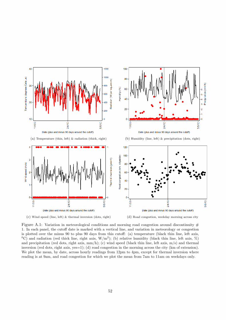
(a) Temperature (thin, left) & radiation (thick, right) (b) Humidity (line, left) & precipitation (dots, right)

(c) Wind speed (line, left) & thermal inversion (dots, right) (d) Road congestion, weekday morning across city

Figure A.1: Variation in meteorological conditions and morning road congestion around discontinuity #1. In each panel, the cutoff date is marked with a vertical line, and variation in meteorology or congestionis plotted over the minus 90 to plus 90 days from this cutoff: (a) temperature (black thin line, left axis,0C) and radiation (red thick line, right axis, W/m2); (b) relative humidity (black thin line, left axis, %)and precipitation (red dots, right axis, mm/h); (c) wind speed (black thin line, left axis, m/s) and thermalinversion (red dots, right axis, yes=1); (d) road congestion in the morning across the city (km of extension).We plot the mean, by date, across hourly readings from 12pm to 4pm, except for thermal inversion wherereading is at 9am, and road congestion for which we plot the mean from 7am to 11am on weekdays only.

52

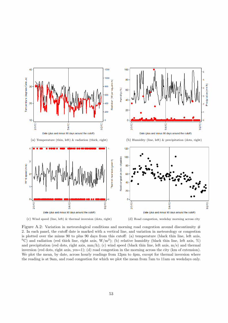
(a) Temperature (thin, left) & radiation (thick, right) (b) Humidity (line, left) & precipitation (dots, right)

(c) Wind speed (line, left) & thermal inversion (dots, right) (d) Road congestion, weekday morning across city

Figure A.2: Variation in meteorological conditions and morning road congestion around discontinuity #2. In each panel, the cutoff date is marked with a vertical line, and variation in meteorology or congestionis plotted over the minus 90 to plus 90 days from this cutoff: (a) temperature (black thin line, left axis,0C) and radiation (red thick line, right axis, W/m2); (b) relative humidity (black thin line, left axis, %)and precipitation (red dots, right axis, mm/h); (c) wind speed (black thin line, left axis, m/s) and thermalinversion (red dots, right axis, yes=1); (d) road congestion in the morning across the city (km of extension).We plot the mean, by date, across hourly readings from 12pm to 4pm, except for thermal inversion wherethe reading is at 9am, and road congestion for which we plot the mean from 7am to 11am on weekdays only.

53

(a) Temperature (thin, left) & radiation (thick, right) (b) Humidity (line, left) & precipitation (dots, right)

(c) Wind speed (line, left) & thermal inversion (dots, right) (d) Road congestion, weekday morning across city

Figure A.3: Variation in meteorological conditions and morning road congestion around discontinuity #3. In each panel, the cutoff date is marked with a vertical line, and variation in meteorology or congestionis plotted over the minus 90 to plus 90 days from this cutoff: (a) temperature (black thin line, left axis,0C) and radiation (red thick line, right axis, W/m2); (b) relative humidity (black thin line, left axis, %)and precipitation (red dots, right axis, mm/h); (c) wind speed (black thin line, left axis, m/s) and thermalinversion (red dots, right axis, yes=1); (d) road congestion in the morning across the city (km of extension).We plot the mean, by date, across hourly readings from 12pm to 4pm, except for thermal inversion wherethe reading is at 9am, and road congestion for which we plot the mean from 7am to 11am on weekdays only.

54

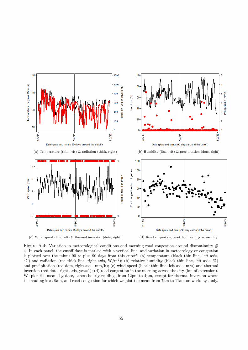
(a) Temperature (thin, left) & radiation (thick, right) (b) Humidity (line, left) & precipitation (dots, right)

(c) Wind speed (line, left) & thermal inversion (dots, right) (d) Road congestion, weekday morning across city

Figure A.4: Variation in meteorological conditions and morning road congestion around discontinuity #4. In each panel, the cutoff date is marked with a vertical line, and variation in meteorology or congestionis plotted over the minus 90 to plus 90 days from this cutoff: (a) temperature (black thin line, left axis,0C) and radiation (red thick line, right axis, W/m2); (b) relative humidity (black thin line, left axis, %)and precipitation (red dots, right axis, mm/h); (c) wind speed (black thin line, left axis, m/s) and thermalinversion (red dots, right axis, yes=1); (d) road congestion in the morning across the city (km of extension).We plot the mean, by date, across hourly readings from 12pm to 4pm, except for thermal inversion wherethe reading is at 9am, and road congestion for which we plot the mean from 7am to 11am on weekdays only.

55

References

Anderson, L. G. (2009). Ethanol fuel use in Brazil: Air quality impacts. Energy & Environmental

Science, 2, pp. 1015-1037.

Angelo, C. (2012). News in Focus: Growth of ethanol fuel stalls in Brazil. Nature, 491, p. 646.

Arceo, E., Hanna, R., Oliva, P. (2016). Does the effect of pollution on infant mortality differ

between developing and developed countries? Evidence from Mexico City. Economic Journal,

126(591), pp. 257-280.

Auffhammer, M., Kellogg, R. (2011). Clearing the air? The effects of gasoline content regulation

on air quality. American Economic Review, 101(6), pp. 2687-2722.

Calonico, S., Cattaneo, M. D., Titiunik, R., (2014a). Robust data-driven inference in the regression-

discontinuity design. Stata Journal, 14(4), pp. 909-946.

Calonico, S., Cattaneo, M. D., Titiunik, R., (2014b). Robust nonparametric confidence intervals

for regression-discontinuity designs. Econometrica, 82(6), pp. 2295-2326.

CBN Noticias (2010). Interview with Dr Jose Goldemberg, former Secretary of the Environment.

Radio interview aired on January 5, 2010, Sao Paulo.

CETESB (2011, 2012, 2013). Relatorio Anual sobre a Qualidade do Ar no Estado de Sao Paulo.

In Portuguese: Annual Report on Air Quality in the State of Sao Paulo. Companhia Ambiental

do Estado de Sao Paulo (Sao Paulo State Environmental Protection Agency), Sao Paulo.

Chen, Y., Ebenstein, A., Greenstone, M., Li, H., (2013). Evidence on the impact of sustained

exposure to air pollution on life expectancy from China’s Huai River policy. Proceedings of the

National Academy of Sciences, 110(32), pp. 12936-12941.

Chicago Tribune (2015). Ald. Burke’s lobbying bonanza ethanol bill is spared under council ‘kill

ordinance’. Reported by John Byrne, May 20.

Cook, R., Phillips, S., Houyoux, M., Dolwick, P., Mason, R., Yanca, C., Zawacki, M., Davidson,

K., Michaels, H., Harvey, C., Somers, J., Luecken, D. (2011). Air quality impacts of increased

use of ethanol under the United States’ Energy Independence and Security Act. Atmospheric

Environment, 45(40), pp. 7714-7724.

Davis, L. W., (2008). The effect of driving restrictions on air quality in Mexico City. Journal of

Political Economy, 116(1), pp. 38-81.

de Gouw, J. A., Gilman, J. B., Borbon, A., Warneke, C., Kuster, W. C., Goldan, P. D., Holloway,

J. S., Peischl, J., Ryerson, T. B., Parrish, D. D., Gentner, D. R., Goldstein, A. H., Harley, R. A.

(2012). Increasing atmospheric burden of ethanol in the United States. Geophysical Research

Letters, 39(15), L15803.

56

Deschenes, O., Greenstone, M., Shapiro, J. S. (2012). Defensive investments and the demand for

air quality: Evidence from the NOx Budget Program and ozone reductions. National Bureau of

Economic Research, Working Paper No. 18267.

Dominici, F., Greenstone, M., Sunstein, C. R. (2014). Particulate Matter matters. Science,

344(6181), pp. 257-259.

Durbin, T. D., Miller, J. W., Younglove, T., Huai, T., Cocker, K. (2007). Effects of fuel ethanol

content and volatility on regulated and unregulated exhaust emissions for the latest technology

gasoline vehicles. Environmental Science & Technology, 41, pp. 4059-4064.

Finlayson-Pitts, B., Pitts, J. (2000). Chemistry of the Upper and Lower Atmosphere: Theory,

Experiments, and Applications. Academic Press, San Diego.

Fujita, E. M., Campbell, D. E., Stockwell, W. R., Saunders, E., Fitzgerald, R., Perea R. (2016).

Projected ozone trends and changes in the ozone precursor relationship in the South Coast Air

Basin in response to varying reductions of precursor emissions. Journal of the Air & Waste

Management Association, 66(2), pp. 201-214.

Gelman, A., Imbens, G., (2014). Why high-order polynomials should not be used in regression

discontinuity designs. National Bureau of Economic Research, Working Paper No. 20405.

Ginnebaugh, D. L., Liang, J., Jacobson, M. Z. (2010). Examining the temperature dependence of

ethanol (E85) versus gasoline emissions on air pollution with a largely-explicit chemical mecha-

nism. Atmospheric Environment, 44(9), pp. 1192-1199.

Hahn, J., Todd, P., Van der Klaauw, W. (2001). Identification and estimation of treatment effects

with a regression-discontinuity design. Econometrica, 69(1), pp. 201-209.

He, J., Gouveia, N., Salvo, A. (2016). The unintended consequences of policies to abate truck flows

inside the Sao Paulo megacity. Mimeo, National University of Singapore and University of Sao

Paulo.

Hochhauser, A. M., Schleyer, C. H. (2014). Summary of Research on the Use of Intermediate

Ethanol Blends in On-Road Vehicles. Energy & Fuels, 28(5), pp. 3236-3247.

Hubbard, C. P., Anderson, J. E., Wallington, T. J. (2014). Ethanol and air quality: influence

of fuel ethanol content on emissions and fuel economy of flexible fuel vehicles. Environmental

Science & Technology, 48(1), pp. 861-867.

Imbens, G. W., Kalyanaraman, K. (2012). Optimal bandwidth choice for the regression disconti-

nuity estimator. Review of Economic Studies 79, pp. 933-959.

Imbens, G. W., Lemieux, T. (2008). Regression discontinuity designs: A guide to practice. Journal

of Econometrics, 142(2), pp. 615-635.

Jacob, D. J. (1999). Introduction to Atmospheric Chemistry. Princeton University Press, Princeton.

57

Jacobson, M. Z. (2007). Effects of ethanol (E85) versus gasoline vehicles on cancer and mortality

in the United States. Environmental Science & Technology, 41(11), pp. 4150-4157.

Jing, P., Lu, Z., Xing, J., Streets, D., Tan, Q., O’Brien, T., Kamberos, J. (2014). Response of the

summertime ground-level ozone trend in the Chicago area to emission controls and temperature

changes, 2005-2013. Atmospheric Environment, 99, pp. 630-640.

Lin, C.-Y. C., Jacob, D. J., Munger, J. W., Fiore, A. M. (2000). Increasing background ozone in

surface air over the United States. Geophysical Research Letters, 27(21), pp. 3465-3468.

Lin, C.-Y. C., Jacob, D. J., Fiore, A. M. (2001). Trends in exceedances of the ozone air quality

standard in the continental United States, 1980-1998. Atmospheric Environment, 35, pp. 3217-

3228.

Lin, C.-Y. C. (2010). A spatial econometric approach to measuring pollution externalities: An

application to ozone smog. Journal of Regional Analysis and Policy, 40(1), pp. 1-19.

Lin Lawell, C.-Y. C., Zhang, W., Umanskaya, V. I. (2016). The effects of driving restrictions on

air quality: Theory and empirical evidence. Mimeo, University of California at Davis.

Ludwig, J., Miller, D. L. (2007). Does Head Start improve children’s life chances? Evidence from

a regression discontinuity design. Quarterly Journal of Economics, 122(1), pp. 159-208.

Madronich, S. (2014). Atmospheric chemistry: Ethanol and ozone. Nature Geoscience, 7, pp.

395-397.

Martins, L. D., Andrade, M. F. (2008a). Emission scenario assessment of gasohol reformulation

proposals and ethanol use in the metropolitan area of Sao Paulo. The Open Atmospheric Science

Journal, 2, pp. 166-175.

Martins, L. D., Andrade, M. F. (2008b). Ozone formation potentials of volatile organic compounds

and ozone sensitivity to their emission in the megacity of Sao Paulo. Water, Air, & Soil Pollution,

195, pp. 201-213.

Martins, L. D., Andrade, M. F., Ynoue,R. Y. (2008). Ambient volatile organic compounds in the

megacity of Sao Paulo. Quim. Nova, 31(8), pp. 2009-2013.

Negri, J. C. (2010). Balanco Energetico do Estado de Sao Paulo. In Portuguese: Energy Balance

for the State of Sao Paulo. Secretaria de Saneamento e Energia do Governo de Sao Paulo (Sao

Paulo State Government, Secretariat for Sanitation and Energy), Sao Paulo.

Nogueira, T., Dominutti, P. A., Carvalho, L. R. F., Fornaro, A., Andrade, M. F. (2014). Formalde-

hyde and acetaldehyde measurements in urban atmosphere impacted by the use of ethanol bio-

fuel: Metropolitan Area of Sao Paulo (MASP), 2012-2013. Fuel, 134, pp. 505-513.

Nogueira, T., Souza, K. F., Fornaro, A., Andrade, M. F., Rothschild, L., Carvalho, L. R. F. (2015).

On-road emissions of carbonyls from vehicles powered by biofuel blends in traffic tunnels in the

Metropolitan Area of Sao Paulo, Brazil. Atmospheric Environment, 108, pp. 88-97.

58

Nopmongcol, U., Griffin, W. M., Yarwood, G., Dunker, A. M., MacLean, H. L., Mansell, G.,

Grant, J. (2011). Impact of dedicated E85 vehicle use on ozone and particulate matter in the

US. Atmospheric Environment, 45(39), pp. 7330-7340.

Orlando, J. P., Alvim, D. S., Yamazaki, A., Correa, S. M. & Gatti, L. V. (2010). Ozone precursors

for the Sao Paulo metropolitan area. Science of the Total Environment, 408, pp. 1612-1620.

Pereira, P. A. P., Santos, L. M. B., Sousa, E. T., Andrade, J. B. (2004). Alcohol- and gasohol-

fuels: a comparative chamber study of photochemical ozone formation. Journal of the Brazilian

Chemical Society, 15, pp. 646-651.

RFA (2016). US Ethanol Industry Outlook. Renewable Fuels Association, Washington, DC.

Salvo, A. (2016). Flexible fuel vehicles, less flexible minded consumers: Price salience experiments

at the pump. Mimeo, National University of Singapore.

Salvo, A., Huse, C. (2011). Is arbitrage tying the price of ethanol to that of gasoline? Evidence

from the uptake of flexible-fuel technology. Energy Journal, 32(3), pp. 119-148.

Salvo, A., Huse, C. (2013). Build it, but will they come? Evidence from consumer choice between

gasoline and sugarcane ethanol. Journal of Environmental Economics and Management, 66, pp.

251-279.

Salvo, A., Geiger, F. M. (2014). Reduction in local ozone levels in urban Sao Paulo due to a shift

from ethanol to gasoline use. Nature Geoscience, 7, pp. 450-458.

Seinfeld, J. H., Pandis, S. N. (1998). Atmospheric Chemistry and Physics: From Air Pollution to

Climate Change. Wiley, New York.

Stedman, D. H. (2004). Photochemical ozone formation, simplified. Environmental Chemistry, 1,

pp. 65-66.

Stephens, S., Madronich, S., Wu, F., Olson, J. B., Ramos, R., Retama, A., Munoz, R. (2008).

Weekly patterns of Mexico City’s surface concentrations of CO, NOx, PM10 and O3 during

19862007. Atmospheric Chemistry and Physics, 8, pp. 5313-5325.

Suarez-Bertoa, R., Zardini, A. A., Platt, S. M., Hellebust, S., Pieber, S. M., El Haddad, I., Temime-

Roussel, B., Baltensperger, U., Marchand, N., Prevot, A. S. H., Astorga, C. (2015). Primary

emissions and secondary organic aerosol formation from the exhaust of a flex-fuel (ethanol)

vehicle. Atmospheric Environment, 117, pp. 200-211.

US EPA (2004). Evaluating Ozone Control Programs in the Eastern United States. United States

Environmental Protection Agency, Office of Atmospheric Programs, Washington, DC.

Wallington, T. J., Anderson, J. E., Kurtz, E. M., Tennison, P. J. (2016). Biofuels, vehicle emissions,

and urban air quality. Faraday Discussions, 189, pp. 121-136.

59