31st Annual Precise Time and Time Interval (PTTI) Meeting

ESTIMATIONOFGPSIONOSPHERICDELAY USINGLlCODEANDCARRIERPHASE

OBSERVABLES

Robert Giffard Agile& Laboratories 3500 Deer Park Rd.

Pao Alto, CA 94304, USA

Abstract

Free electrons in the earth’s ionosphere cause a frequency-dependent group delay in the bands used for the spread- spectrum GPS ranging signals. This delay constitutes a potential source of error in timing measurements. The ionospheric delay can be removed by dual-frequency ranging using the Ll and L2 signals. Two-frequency time receivers are currently expensive, and are not very reliable when tracking low elevation satellites when Anti- Spoofing is enabled, unless decryption can be used. Single-frequency, Ll, receivers can correct for the delay using a detailed model of the ionosphere scaled by data contained in the ‘navigation message’ broadcast by the satellites. However, because of unpredictable variations of the ionosphere, this so-called single-frequency correction is only expected to absorb 50% of the effect. The uncorrected ionospheric delay can cause significant errors in LI timing systems such as disciplined oscillators. This unpredictable source of error is of increasing importance with the approach of the solar activity maximum. Estimates of the ionospheric delay, calculated from two-frequency geodesic measurements, are now available from several sources, but these are not easy to apply in real time. In the future, WAAS and other system real-time ionosphere estimates for some geographical areas will be available with suitable receivers via geostationary satellites. We report attempts to model the zenith ionosphere correction from observations of the Ll code and cam’er phase GPS observables made with a multi-channel receiver module. Code and carrier phases are affected by dispersion with opposite signs, but carrier phase always contains an ambiguity. It will be shown that by measuring derivatives of the observables, the ionospheric delay can be estimated approximately by post-processing the output of a single-frequency receiver. The use of a single frequency avoids inaccuracy due to group delay differences in the receiver for LI and L2 signals. Real-time estimation could be performed if the batch processing procedure were replaced by a suitable filter. Preliminary results will be presented, and compared with post-processed IGS estimates.

1 INTRODUCTION

One-way time transfer using the Global Positioning System constitutes a convenient method of comparing local time scales with UTC(USN0 MC). GPS-disciplined oscillators (GPSDOs) that provide an autonomous time output using this technique are now widely used. Civilian GPS users have to contend with the intentional randomization of the satellite clocks by ‘Selective Availability’ (SA), but if the measurements can be averaged for 1 - 2 days, the rrns uncertainty is reduced to about 1 ns. We have shown elsewhere [l] that ionospheric dispersion appears to cause errors of up to 25 ns in one-way time transfer with the single- frequency receivers typically used in GPSDOs, even when the built-in ionosphere correction is used.

Worldwide estimates of the ionospheric delays are now available from the IGS and others, but these cannot be used with GPSDOs because of the computational delays of 3-7 days and the day-to-day variability of the ionosphere. It is also inconvenient if an external communication link is required at each GPSDO site. Since two-frequency time receivers that can correct for the ionosphere are not widely available, it would be very useful if a stand-alone single-frequency receiver could form a useful estimate of the local effect and correct for it in real time. Determination of the ionospheric delay by post-processing using a single-frequency receiver has previously been demonstrated [2]. Single-frequency methods of ionosphere determination avoid uncertainties associated with satellite and receiver interfrequency biases.

405

Report Documentation Page Form ApprovedOMB No. 0704-0188

Public reporting burden for the collection of information is estimated to average 1 hour per response, including the time for reviewing instructions, searching existing data sources, gathering andmaintaining the data needed, and completing and reviewing the collection of information. Send comments regarding this burden estimate or any other aspect of this collection of information,including suggestions for reducing this burden, to Washington Headquarters Services, Directorate for Information Operations and Reports, 1215 Jefferson Davis Highway, Suite 1204, ArlingtonVA 22202-4302. Respondents should be aware that notwithstanding any other provision of law, no person shall be subject to a penalty for failing to comply with a collection of information if itdoes not display a currently valid OMB control number.

1. REPORT DATE DEC 1999 2. REPORT TYPE

3. DATES COVERED 00-00-1999 to 00-00-1999

4. TITLE AND SUBTITLE Estimation of GPS Ionospheric Delay Using L1 Code and Carrier Phase Observables

5a. CONTRACT NUMBER

5b. GRANT NUMBER

5c. PROGRAM ELEMENT NUMBER

6. AUTHOR(S) 5d. PROJECT NUMBER

5e. TASK NUMBER

5f. WORK UNIT NUMBER

7. PERFORMING ORGANIZATION NAME(S) AND ADDRESS(ES) Agilent Laboratories,3500 Deer Park Rd,Palo Alto,CA,94304

8. PERFORMING ORGANIZATIONREPORT NUMBER

9. SPONSORING/MONITORING AGENCY NAME(S) AND ADDRESS(ES) 10. SPONSOR/MONITOR’S ACRONYM(S)

11. SPONSOR/MONITOR’S REPORT NUMBER(S)

12. DISTRIBUTION/AVAILABILITY STATEMENT Approved for public release; distribution unlimited

13. SUPPLEMENTARY NOTES See also ADM001481. 31st Annual Precise Time and Time Interval (PTTI) Planning Meeting, 7-9December 1999, Dana Point, CA

14. ABSTRACT see report

15. SUBJECT TERMS

16. SECURITY CLASSIFICATION OF: 17. LIMITATION OF ABSTRACT Same as

Report (SAR)

18. NUMBEROF PAGES

13

19a. NAME OFRESPONSIBLE PERSON

a. REPORT unclassified

b. ABSTRACT unclassified

c. THIS PAGE unclassified

Standard Form 298 (Rev. 8-98) Prescribed by ANSI Std Z39-18

In this paper, we describe experiments that have been carried out to demonstrate the estimation of the local ionospheric delay using Motorola ‘ONCORE-VP’ &channel,-modular Ll time receivers. The raw data from the receivers wereprocessed on-line by an external measurement computer in order to obtain simultaneous code range and carrier-phase data samples related to the receiver’s internal clock. Estimates of the local average ionosphere delay were obtained in these experiments by subsequent off-line block-mode computation, but a real-time estimate could be obtained using suitable algorithms. The datawere compared with the estimates from various processing centers through the data-base of the IGS, and agreement was found to be satisfactory. For diagnostic purposes, it was found useful to phase-lock the receiver clock oscillator to a stable external frequency reference, but this is not required in principle. It was also found useful to reduce multipath effects using a choke-ring antenna.

The model of receiver used in the experiments is now obsolete, but we feel that the technique demonstrated is general and useful, and could be used with other receivers.

2 EFFECT OF IONOSPHERE ON Ll TIME TRANSFER

The presence of free electrons in the Earth’s ionosphere leads to significant dispersion at the GPS Ll and L2 frequencies [3]. The effect , in first order, is to cause the group velocity to be reduced, and the phase velocity to be increased by equal amounts. The receiver measures the range to a given satellite by code and phase tracking loops. The code tracking loop estimates the code range, p&e, given by:

pcode = pt + C X du - C X 4 + Ptropo + Piano + Mc- (1)

The output of the phasetracking loop depends on the phase range, pphase, given by:

Pphase = pt + C X du - C X 4 + Ptropo - Piano + Mp (2)

In these equations, pt is the true geometric range to the satellite, the receiver and satellite clock biases are d,

and d, respectively, ptropo is the path increase due to the troposphere, piono is the path increase equivalent to

the ionospheric group delay, and c is the speed of light. The quantities M, and M, are code and phase errors due to multipath. The troposphere path increase is non-dispersive, and affects code and phase equally.

The theoretical path increase piono due to the effect of dispersion in the ionosphere is given [3] by:

piono = 40.3 x TEC ! f ‘9

where TEC is the total free electron content integrated along the line of sight to the satellite in units of electrons per rn’, f is the frequency in Hz, and piono is in meters. TEC varies with time, and depends on the

location in the ionosphere ‘pierced’ by the line of sight to the satellite. Equation (3) shows how the ionosphere effect depends on frequency.

At the Ll frequency, 1575.42 MHz, Equation (3) can be written for a satellite that is not at the zenith:

Piono = 0.162 X F X TEC,. (4)

In Equation (4), TEC, is the TEC value for a vertical column located at the pierce point, in units of lOI electrons per rn’, and F is an obliquity factor for the line of sight to the satellite. Assuming that the active region of the ionosphere can be represented by a thin shell at an elevation of 350 km, the obliquity can be

406

approximately expressed [4] as a simple function of the elevation angle in degrees, E, of the satellite at the receiver’s antenna:

F= 1 + 2.74 x 10-6(96 - E)‘. (5)

The complex spatial and temporal variation of TEC has been extensively studied. The most obvious feature is a cyclic, daily variation. The average amplitude of the daily peak and its duration change with the season of the year, the phase of the solar cycle, and the geomagnetic latitude of the observer. There is also considerable day-to-day variability associated with solar activity. In order to estimate the ionosphere effect for one-way time transfer, both the value of TEC and the value of F averaged over the visible satellites must be known. For a receiver with a minimum elevation angle set to 15 degrees, this has been found to be about 1.8 at the latitude of the experiments to be described. Since the local TEC value can reach 75, average peak delays of 70 ns may be expected. The average delay at night falls to a minimum of about 9 ns, so that there is a strong day-night difference in the raw delay.

Conventionally, dual-frequency receivers are used to determine the ionosphere effect by observing the code ranges at the GPS L 1 and L2 frequencies. Equations (1) and (3) can be used to calculate Piono directly, or the

data can be used to calculate an ‘ionosphere-free’ range [5]. Two-frequency receivers are significantly more complex and expensive, and the presence of the Y-code makes L2 tracking harder for non-DOD users. Compensation for the ionosphere effect determined in this way can also increase noise, and reduces the reliability of the measurements made by a stand-alone user.

The GPS system navigation message contains a correction that single-frequency receivers can use to compensate for the ionosphere effect in real time [4,6]. The correction emulates the spatial and time variation with an amplitude that is adjusted depending on observed solar radiation flux. Using the broadcast correction is expected to reduce the ionosphere effect in an Ll receiver by a factor of at least 2.0 [7].

Equations (1) and (2) suggest that the ionosphere effect might be measured by observing both the code and carrier ranges. If we calculate the code minus carrier difference, we obtain:

P code - pphase = 2 . fkmo +Mc- Mp +nh/2. (6)

In Equation (6), the term t&/2 shows that the carrier phase measurement is ambiguous by an integer number of half wavelengths [S]. The multipath effects in the code range are generally much larger than those in phase. As long as the receiver phase-locked loops track continuously, n remains constant. Any dispersion in the receiver system will also cause unknown, but ideally constant, offsets. Because of the integer ambiguity inherent in carrier phase measurements, Equation (4) cannot be used to determine pion directly. During continuous phase trackin g, however, it should be possible to use the time dependence of the code-carrier difference to estimate Piano.

A complete model of the time and spatial dependence of the ionospheric dispersion given inEquation (3) is complicated. As an approximation, we will assume that the density of the ionosphere is uniform over the region sampled by the lines of sight to the satellites from the receiver, and varies with time. The simplifying assumption of local spatial uniformity should be completely acceptable in the context of time transfeq because only an average of the ionosphere delay over all visible satellites is required.

Combining Equations (4) - (6) and introducing explicit time dependence, we expect the code-carrier path difference for the ith satellite, Ai, to vary as:

4 = (Pcode - pphase)i = 0.325 X Fi(t) X TECJt) + n&2 + Ei. (7)

407

By differentiating Equation (7) for each of N satellites, with the assumption that there are no phase slips, we

obtain the set of N equations in TEC,, and its derivative, TEC, ‘:

Ai ’ / 0.325 = F, X TEC, ’ + Fi ’ X TEC, + V1

. . . . . . . . . . . . . . . . . . . . . (8)

Ai’ / 0.325 = FN x TEC, ’ +FN’ x TEC, + vN

The terms vi through vN correspond to noise and errors in the derivatives of the code-carrier differences.

Since the values of Fi and the derivatives Fi ’ are known, the rates of change of the code-carrier differences

can, in principle, be used to estimate TEC, and its first derivative by inverting the set of Equations (8). If more than 2 satellites are tracked, a least-squares solution can be obtained using the pseudoinverse. When

calculating the derivatives Ai ’ only data obtained without phase slips can be used.

3 EXPERIMENTAL DETAILS

The Motorola ONCORE-VP receiver can output serial data containing the values, at an internally defined measurement epoch, of code and carrier phase for all satellites tracked. Measurement epochs take place approximately once per second. To obtain the code-carrier differences as a function of time, it is necessary to understand the operation of the receiver in some detail.

OBTAINING RAW GPS OBSERVABLES Signal processing in the Motorola ONCORE-VP is conerent with the receiver’s crystal oscillator, which has a nominal frequency F0 of 19,095,750 Hz. The receiver front-end down-converts the satellite carrier frequency F, to a final baseband frequency Fb given by:

Fb = Fc - 82.5 x F,,. (9)

In Equation (9), F, is given by:

F, = 1,575.42 x lo6 + Fd. (10)

In these equations, Fd is the Doppler frequency shift caused by motion of the satellite and the receiver. It can be seen from Equations (9) and (10) that the baseband frequency is equal to Fd plus the difference between the receiver oscillator and 19.096 MHz, ‘multiplied by 82.5. For the nominal oscillator frequency, the baseband frequency is 20,625 + Fd Hz.

The receiver tracks the carrier phase of up to 8 satellites using software phase-locked loops. These loops operate at the baseband frequency. Each phase sample latched by the receiver at the measurement epoch is the integral from an arbitrary starting time of the frequency Fb obtained by substituting Equation (10) into Equation (9). The phase samples are reported modulo 65,536 cycles, and it is necessary to sample about once each second and keep track of rollovers.

The receiver code cot-relator measures the phase of the pseudo-random CA code for up to 8 satellites using software delay-locked loops operating at the baseband frequency. The output values are the phases of the code NCOs, sampled at the measurement epoch. Dithering and interpolation are used to resolve less than a single unit of NC0 phase. The code phase samples are modulo 1,575,420 cycles, and data from the navigation messageareused to remove the resulting millisecond ambiguities.

408

The code-carrier range difference at each measurement epoch is obtained by subtracting the integral of the Doppler shift Fd multiplied by the wavelength from the code range. It appears from the frequency and time relationships discussed above that the Doppler integral has to be corrected for the integral of the baseband offset, and the code phase has to be corrected for the time delay of the epoch. However, when the code phase and the integrated Doppler shift are both expressed as ranges, these two corrections are the same. It follows that code-carrier range differences can be obtained without precise knowledge of the receiver clock frequency offset.

RECEIVER OSCILLATOR PHASE STABILIZATION

It is convenient to be able to use the continuity of the carrier-phase readings to check for phase slips. Because of the nature of the tracking loops, the smallest phase jump that can be caused by a noise transient is half a cycle, corresponding to a time of about 300 ps. To detect jumps, the rms phase run-out of the receiver clock oscillator between adjacent carrier-phase samples must therefore be much smaller than 300 ps. This corresponds to an Allan variance at 1 s of 3 x lo-“. The free-running noise of the receiver’s crystal oscillator is much larger than this.

To obtain single-satellite carrier phase data and detect phase slips, the receiver’s clock offset must be stabilized. This was done in these experiments by phase-locking the receiver’s TCXO to an external stable reference, an HP 5061B cesium standard. A simple ‘m/n’ division technique and a low-noise linear phase detector were used to lock the oscillator to a frequency of 3590/188 MHz, resulting in a baseband offset of 21,063.8297873 Hz. The loop filter has an overall loop time constant of about 0.1 second.

MEASUREMENT CO-PROCESSOR

The serial output data of the GPS receiver were fed each second to an external measurement co-processor. The signal processing program calculated the raw code and phase ranges referred to a smooth clock derived from the external oscillator. The readings were subtracted to give the code-carrier difference. Correct results required that the data from the receiver be processed each second. All the adjustments and corrections described above were carried out on-line. The resulting data werefed to digital low-pass filters, and the output for up to 8 satellites was filed on a UNIX file server each 15 seconds. The data included a UTC time- stamp and, for each satellite: PRN, elevation, azimuth, SNR, the loss-of-lock flag, and the integrated Doppler shift. The datawerefiled in 12-hour segments, and about 2 Mbytes of datawereobtained each day in the form of ASCII files. The values of code and phase delays were propagated to integer UTC seconds using the measured Doppler frequencies.

To check the overall phase stability, raw carrier phase data were recorded each second from a chosen satellite. The average Doppler shift was obtained by subtracting successive readings, and the Doppler values were adjusted for the epoch spacin g, and fed to a digital filter that tracked the average value and the first derivative with a time constant of about 5 seconds. The filter output was processed to obtain the difference between the Doppler value and the value predicted by the filter for the same time. The rms of these values was found to be approximately 0.03 cycles under ideal conditions.

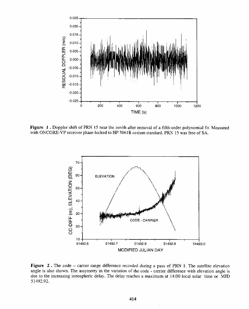
Figure 1 shows a lOOO-second section of Doppler residuals calculated from data recorded using the phase- locked receiver. The satellite was PRN 15, which showed no detectable SA. The data were recorded near a minimum in carrier phase, and a fifth-order fit to the time-varying Doppler shift has been subtracted in Figure 1 . The remaining deviation is due to phase noise in the receiver and the satellite signal, and quantization error in the receiver data messages. The total rms noise is 0.0053 m/s, corresponding to an L2 carrier phase error of 0.03 cycles at each measurement epoch. The phase stability corresponds to an Allan variance in frequency of about 2.0 x lo-” at 1 second, and an rms range noise of 6 mm for phase at each sample.

409

Data such as that shown in Figure 1 show that the receiver, with its oscillator phase-locked to the external reference, is stable enough for the l-second Doppler differences to be used as a check of continuous phase tracking. In fact, the receiver itself has an output signaling phase hits, and this was OR’d with the output of a discriminator on the Doppler filter in the experiments to be described. The discriminator was set to flag Doppler residuals of more than 0.4 cycles per second.

MULTIPATH ERRORS

As discussed above, the code-carrier difference is affected by multipath. This occurs because the code correlator is much more sensitive to multipath than the carrier-phase-lock loop. The ratio of sensitivity is approximately equal to the ratio of the length of a code chip in space, 300 m, to the’carrier wavelength, 0.19 m. Multipath noise can be recognized by the fact that it repeats each sidereal day for a given satellite. This noise is undesirable as it reduces the accuracy of the fitting procedure expressed in Equations (8). Various antenna types were used in the course of the experiments. The final data were taken using a choke-ring antenna that seemed to reduce the multipath effects significantly. The type of antenna used is also known to have good phase center stability.

Figure 2 shows the raw code-carrier difference and the satellite elevation angle recorded during a pass of PRN 1. This pass began during the local night, when the TEC value is comparatively small, and constant. During the second half of the pass, the ionospheric delay increased to its daily maximum, causing a strongly asymmetric variation of the code-carrier difference,in contrast with the variation of the satellite elevation. The data also show a degradation of the noise level at the ends of the track due to decreasing signal strength and increasing susceptibility to multipath. The code-carrier difference is not affected by SA.

OFF-LINE DATA PROCESSING During the experiments, dataweretaken continuously and processed later. This allowed various algorithms to be developed and tried on the same. raw data. The data for each daywere divided into 64 overlapping blocks of length 2700 s, each containing 180 15second samples. “The average rate of change of the code-carrier difference for a given satellite, within each block, was determined by a linear regression through all the points in the block. The obliquity factor for the satellite was calculated from the elevation angle using Equation (5), and a linear regression was used to determine the average and the average rate of change during the same period. The data for a given satellite wereonly considered valid if the loss-of-lock status flag indicated that the carrier phase was tracked continuously during the block.

For each data block, up to 8 valid sets of values of Ai ‘, F;, and Fi ’ could be obtained. These were then used

to obtain a minimum-squares solution for TEC, and the rate of change TEC,’ for each block using the

pseudoinverse method. The uncertainty in the solution depends on the noise level on the code-carrier differences. The noise on the derivatives is reduced by extending the time over which the slope is estimated, but this cannot be too long because of the higher order time dependence of TEC, and Fi. These considerations led to the choice of 2700 s for the block length.

The functional relationship between TEC, and its derivative can also be used to improve the accuracy of the

estimate of TEC,. The 64 TEC, values obtained per day were smoothed using the TEC, ’ values by means of

a simple recursive algorithm of the following form:

Sj = (1 - K) (Sj_1 + At X Tj ‘) + K X Tj. (11)

In Equation (1 l), Sj is the value of the estimate of TEC, after step j, At is the time step, Tj ’ is the calculated

value of TEC, ’ for step j, Tj is the value of TEC, for step j, and K is a constant smaller than 1. Values of K

between 0.3 and 0.03 gave good results.

410

4 RESULTS AND DISCUSSION

Code-carrier data covering more than 40 days at various times during 1998 and 1999 has now been successfully recorded and analyzed using the method described above.

Figure 3 shows three days of data for the location of Agilent Laboratories, Latitude 37.4, Longitude -

122.2. The two curves show the values of TEC, and the rate of change, TEC, ‘, obtained by solving

Equations (8). An average of about 5.5 valid data blocks was available at each point and all the datawere equally weighted. The units are TEC-units and TEC-units-per-day respectively. Figure 4 shows the smoothed estimate of TEC, obtained from the same data using the filter represented by Equation (11) with a K value of 0.1. The smoothing is obviously quite effective.

A maximum day-to-night variation of 55 TEC units is seen, corresponding to a time-transfer offset variation of 53 ns for a typical satellite constellation. The average of the TEC, value over three days is 24, corresponding to an average uncorrected time error of 23 ns.

Several computation centers of the IGS now calculate explicit estimates of the worldwide variation of the ionospheric delay. Data from over 100 geodetic dual-frequency receiversarecollected centrally and used to calculate precise satellite orbits. This orbit dataarethen used for post-processing in high-resolution geodesy experiments. The ionospheric delay estimates are produced as by-products of the fitting algorithms used for orbit determination. The IGS ionosphere dataareavailable in ‘IONEX’ maps with a resolution of 2.5 degrees in latitude, and 5 degrees in longitude. The time step between maps is 2 hours, but accurate interpolation is possible using the fact that the ionosphere is relatively stationary in solar geocentric coordinates. The dataare available 3-7 days after the observations.

In Figure 5 the single-frequency average TEC, data obtained experimentally arecompared with IGS data. The 3-day period covered is the same as that in Figure 3 . The IGS data from several source:have been used to calculate the time variation at the latitude and longitude of the experiments using the suggested interpolation procedure [9]. The single frequency data agree with the IGS data to within the scatter of the IGS data from various processing centers. The agreement with the data from the Center for Orbit Determination in Europe, Beme, is particularly good: the average and rms differences over the 3-day period are equal to -1 .O and 3.5 ns respectively.

It should be noted that the IGS products assume an ionospheric height of 450 km, which differs from the value of 350 km implicit in the use of the approximate obliquity expression, Equation (5). It is not clear at present how much this affects our results. Figure 6 shows the single-frequency data calculated over a period of 16 days between MJD 51487 and 51503. The peak TEC, values can be seen to vary considerably over the period of a few days.

5 SUMMARY

Algorithms have been developed that allow the local vertical ionospheric delay to be determined using the GPS observables from a multi-channel, single-frequency receiver. Simultaneous measurements on several satellites are used to overcome the cycle-ambiguity of carrier-phase measurements. The algorithm assumes that the ionosphere is spatially uniform over the area sampled by the satellites. This is a relatively simple and inexpensive way of obtaining ionosphere data of moderate quality in real time. The single-frequency method is independent of receiver and satellite inter-frequency biases. Because the receiver is not required to track the L2 signal in the presence of PN code, the trackin g is not upset by rapid scintillation or poor signal strengths at low elevations.

411

The TEC, data obtained by the procedure described abovehave been found to lie remarkably close to the post-processed IGS estimates. The degree of agreement between these results and the IGS data for the same position seems to be between 10 and 20%. This is approximately the level to which the IGS estimates agree amongst themselves. A filter could be designed to estimate the rate of change of the code-carrier difference for each satellite tracked in real time, which would, in turn, enable the TEC, value to be estimated in real time. This could be used with a calculated average obliquity factor to compensate the output of a time receiver directly for ionospheric delay. This should reduce the short= and long-term offsets seen [l] in one- way time transfer by a factor between 3 and 10.

The algorithms that were used to obtain these results were not optimized, and accuracy improvements could possibly be obtained by changing the block size, or by weighting the code-carrier difference data according to signal-to-noise ratio. A better understanding of the noise would also enable an optimum choice of the filter constant to be made. Further analysis of the impact of the approximations used in the processing algorithms would allow the ultimate accuracy of the method to be estimated. It would be very interesting to repeat the measurements usin g a receiver using narrow correlator spacing, or some other technique, to reduce the effect of multipath.

Further work should be directed to analyzing the effects of the spatial uniformity assumption and the block size on the accuracy of the TEC, estimate. The use of .a more accurate obliquity function might be helpful. It might be possible to trade some signal to noise against the introduction of spatial derivatives in the algorithm. A demonstration of the improvement in time- transfer accuracy resulting from real-time application of the autonomous TEC, estimates should be carried out.

ACKNOWLEDGMENTS

It is a pleasure to acknowledge the encouragement of Len Cutler of Agilent Laboratories, Al Gifford of NIST, and Tom Bartholomew of TASC. Many useful interactions with Mike King of Motorola helped us to get the best out of the very versatile GPS receivers.

6 REFERENCES

[l] R.P. Giffard and R. Pitcock, “Comparison of Common-View and One-Way GPS Time Transfer Over a 4000 km East-West Baseline:’ presented at the 3 1” Annual Precise Time and Time Interval (PTTI) Systems and Applications Meeting, California, December 1999.

[2] C.E. Cohen, B. Pervan, and B .W. Parkinson, “Estimation of Absolute Ionospheric Delay Exclusively through Single-Frequency GPS Measurements:’ in Proceedings of ION GPS-92, Institute of Navigation 1992, pp. 325330.

[3] J. A. Klobuchar, “Ionospheric effects on GPS,” in Global Positioning System: Theory and Applications, Vol., Editors: B.W. Parkinson and J.J. Spilker, Progress in Astronautics and Aeronautics, Vol. 163, pp. 48.5-515.

[4] J.A. Klobuchar, “Design and Characteristics of the GPS Ionospheric Time Delay Algorithm for Single Frequency Users;’ in Proceedings of the IEEE Position, Location, and Navigation Symposium, Las Vegas, NV, USA, Nov. 1986, pp. 280-286.

[5] J.J. Spilker, “GPS Navigation Data:’ in Global Positioning System: Theory and Applications, Vol.1, Editors: B.W. Parkinson and J.J. Spilker, Progress in Astronautics and Aeronautics, Vol. 163, pp. 121-176.

412

[6] J.A. Klobuchar, “Present Status and Future Prospects for Ionospheric Propagation Corrections for Precise Time Transfer Using GPS,” in Proceedings of the 23rd Annual Precision Time and Time Interval (PTTI) Applications and Planning Meeting (NASA Conference Publication 3 159), 1991, pp. 417-427.

[7] GPS Zntellface Control Document ZCD-GPS-200, Revision IRN-200C-002, Arinc Research Corporation, 10 Oct. 1993, pp. 124-127.

[8] A.J. Van Dierendonck, “GPS Receivers:’ in Global Positioning System: Theory and Applications, Vol.1, Editors: B.W. Parkinson and J.J. Spilker, Progress in Astronautics and Aeronautics, Vol.

163, pp. 329-407.

[9] S. Shaer and J. Feltens, “IONEX: The IONosphere Map Exchange Format Version 1:’ in Proceedings of the IGS Workshop, Darmstadt, Germany, February 1999.

413

0.025

0.020-

0.015 -

0.010 -

0.005-

0.000 -

-O.OO,: -0.010 -0.015 -

-0.020 -

-0.025 I I 1 I I 0 200 400 600 800 1000 1:

TIME (s)

00

Figure 1 . Doppler shift of PRN 15 near the zenith after removal of a fifth-order polynomial fit. Measured with ONCORE-VP receiver phase-locked to HP 5061B cesium standard. PRN 15 was free of SA.

60- ELEVATION

10 I I I I 51492.6 51492.7 51492.8 51492.9 51493.0

MODIFIED JULIAN DAY

Figure 2 . The code - carrier range difference recorded during a pass of PRN 1. The satellite elevation angle is also shown. The assymetry in the variation of the code - carrier difference with elevation angle is due to the increasing ionospheric delay. The delay reaches a maximum at 14:OO local solar time or MJD 5 1492.92.

414

Figure 3. Values of TEC, and the derivative TEC,’ calculated from 3 days of single-frequency measurements. The values of TEC, ’ are scaled in TEC units per hour, and have been displaced -20 units for

clarity.

70 CALCULATED TEC 60

50

40

30

20

10

0

-10

-20

I-- -30

80,

-40 ' , I I 1 I I I 51492.5 51493.0 51493.5 51494.0 51494.5 51495.0 51495.5

MODIFIED JULIAN DAY

80

70- SMOOTHED TEC

60-

P 50-

z 0 40- P - 30-

ti I- 20-

10-

0, 51492.5 51493.0 51493.5 51494.0 51494.5 51495.0 51495.5

MODIFIED JULIAN DAY

Figure 4 . The smoothed estimate of the single-frequency, measured, vertical TEC calculated from the data shown in Figure (3) using Equation (11) with a K-value of 0.1. The location of the receiver is: Latitude 37.4, Longitude -122.15.

415

80 CALCULATED VERTICAL TEC AND IGS PRODUCTS

, 70 -

6-f k 60-

2 Y 50-

t.

E

40-

: 30-

i= 20-

: lo-

51492.5 51493.0 51493.5 51494.0 51494.5 51495.0 51495.5

MODIFIED JULIAN DAY

Figure 5 . The smoothed, single-frequency, local average TEC, (solid line) calculated from the data shown in Figure 3 , compared with vertical TEC estimated for the same position constructed using IGS product data. Open squares: Center for Orbit Determination for Europe, Bern. Open circles: Jet Propulsion Laboratory, Pasadena, CA. Open triangles: National Resources, Canada.

90 ESTIMATED VERTICAL TEC (LAT 37.4, LOG -122.15)

80

E

70

z 60

1 ti 50

t. 40

0 r 30

20

10

51486 51488 51490 51492 51494 51496 51498 51500 51502 51504

MODIFIED JULIAN DAY

Figure 6 . Two weeks of the estimated vertical TEC in TEC-units at the location of Agilent Labs in Palo Alto, CA. The TEC is estimated from local measurements of the GPS, Ll, code-carrier range difference using the algorithms described in the text.

416

Questions and Answers

DEMETRIOS MATSAKIS (USNO): I just want to say that we have seen at the Observatory fluctuations of up to 10 nanoseconds that we could explain by using IGS maps instead of model ionosphere. And that would bring our two frequency receivers in line with our one. I just wondered if you could turn those numbers that you have for TEC into a numerical difference?

ROBIN GIFFARD (Agilent Technologies): According to nanoseconds. Yes, it’s .54 nanoseconds per TEC unit.

MATSAKIS: So, the difference between the two sites -

GIFFARD: The rms’s for mine, yes, were less than a nanosecond. I’m sorry, I should have explained that.

4171418