Estimation Theory Basics What is Estimation best something...

EE 5510 Random Processes E - 1

Estimation Theory Basics

What is Estimation

Make a best determination ofsomething given measurements(information) related (in a known,or partially known way) to thatsomething, and possibly also givensome prior information

Prior Information may be

• a Random Variable, this is the Bayesian Approach,

• non-random, or sets

Example: Estimation of the mean of random variable:

mx =1

n

n∑i=1

Xi

is an estimator formx = E(X), the mean of the random variableX.We know that mx is a “good” estimator, since

P (|mx −mx| < ε)→ 1

by the law of large numbers.


Parameter Estimation

We are given a number of observations xi, i.e., x = [x1, x2, · · · , xn]. Thissample vector of “data” is called a statistic. From this statistic we areto estimate the desired parameter, i.e.,

θ = g(x)

Unbiased EstimatorAn estimator is unbiased if

E(θ) = θ

Example: The estimator mx = 1n

∑ni=1 xi is an unbiased estimator since

E(mx) =1

n

n∑i=1

E(xi) = mx

Example: Estimation of unknown variance (and unknown mean):

σ2 =1

n− 1

n∑i=1

(xi − mx)2

This estimator is unbiased, since

E((xi − mx)

2) = E(x2i )− 2E

(1

nxi

n∑j=1

xj

)+ E

(1

n2

n∑j=1

n∑i=1

xixj

)

= E(x2i )− 2

1

nE(x2

i )− 2n− 1

nm2x

+1

n2

n∑j=1

E(x2j) +

n(n− 1)

n2 m2x

= E(x2i )

(1− 1

n

)− n− 1

nm2x

= σ2n− 1

n


Biased Coin TossAssume that a coin is biased and shows head (=1) with probability θ 6=0.5, and tail with probability 1− θ. We observe the n tosses of this coinand are to estimate the probability θ of a head toss.Let us form the statistic

z =x1 + x2 + · · ·+ xn

n

The mean of this estimator is

E(Z) =1

n

n∑i=1

E(Xi) = θ

and hence this estimator is unbiased.The variance of this estimator is

σ2z = E

((Z − θ)2)

= E

(1

n2

n∑i=1

n∑j=1

XiXj

)− 2E

(1

n

n∑i=1

Xiθ

)+ θ2

= E

(1

n2

n∑i=1

n∑j=1

XiXj

)− θ2

=n− 1

n(n(n− 1)θ2 − nθ)− θ2 =

θ(1− θ)n

The question arrises whether this is the “best” estimator?

Minimum Variance Estimators (MVE)

Let us find the estimator which minimizes E(

(θ − θ)2)

However the MVE cannot, in general, be determined, since

E(

(θ − θ)2)

= E(

(θ − E(θ)− (θ − E(θ))2)

= (θ − E(θ))2 + var(θ)

since the term (θ − E(θ))2, called the bias, depends on the unknownquantity θ.


Cramer-Rao Lower Bound

AssumptionsWe assume that we have knowledge of the parametric distribution f(x, θ),and that this distribution is differentiable with respect to θ. We also as-sume that the domain of the statistic x does not depend on the parameterθ.DerivationWe now concentrate on unbiased estimators:

E(θ − θ) =

∫(θ − θ)f(x, θ)dx = 0

due to the unbiased nature of θ. Now

d

dθ

∫(θ − θ)f(x, θ)dx =

∫d

dθ(θ − θ)f(x, θ)dx

= −∫f(x, θ)dx+

∫(θ − θ) d

dθf(x, θ)dx = 0

Using the identity

d

dθf(x, θ) =

d ln(f(x, θ))

dθf(x, θ)

we develop:

1 =

∫(θ − θ)d ln(f(x, θ))

dθf(x, θ)dx

≤∫

(θ − θ)2f(x, θ)dx

∫ (d ln(f(x, θ))

dθ

)2

f(x, θ)dx

from which we find the Cramer-Rao lower bound (CRLB):

var(θ) ≥ 1

E(d ln(f(x,θ))

dθ

)2


Equality in the CRLB is achieved if equality is achieved in the Schwarzinequality (see Page ??) used to prove it, i.e., if

d ln(f(x, θ))

dθ= I(θ)(θ − θ)

I(θ) =

∫ (d ln(f(x, θ))

dθ

)2

f(x, θ)dx

= −∫d2 ln(f(x, θ))

dθ2 f(x, θ)dx

is the Fisher Information of θ contained in the observation x. Example:

Consider n observations of a constant A in Gaussian noise, i.e.,

xi = A+ ni; 1 ≤ i ≤ n

The PDF of the observation vector x = (x1, · · · , xn) is given by

f(x, A) =1

(2πσ2)(n/2) exp

(− 1

2σ2

n∑i=1

(xi − A)2

)We calculate

d ln(f(x, A))

dA=

1

σ2

n∑i=1

(xi − A) =n

σ2

(1

n

n∑i=1

xi − A)

from which we can identify the optimal unbiased estimator as

A =1

n

n∑i=1

xi

Furthermore

d2 ln(f(x, A))

dA2 = − n

σ2 = −I(A)

and the variance of the estimator is given by

var(A) =1

I(A)=σ2

n


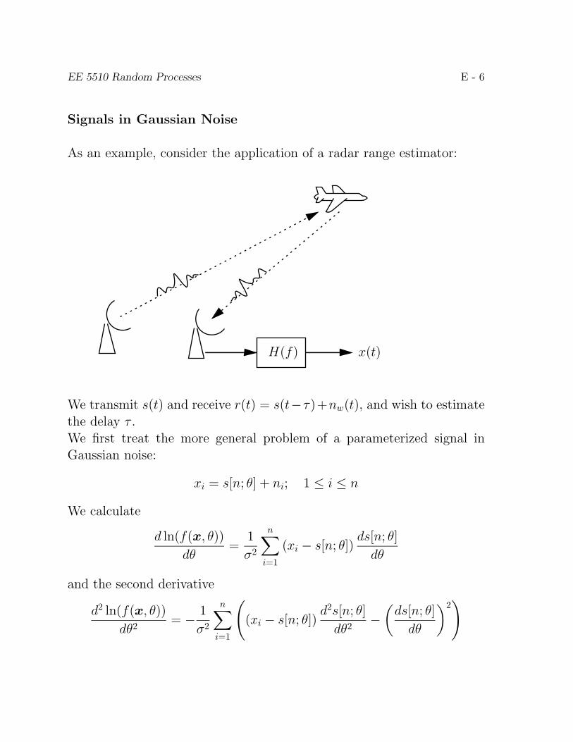
Signals in Gaussian Noise

As an example, consider the application of a radar range estimator:

H(f) x(t)

We transmit s(t) and receive r(t) = s(t−τ)+nw(t), and wish to estimatethe delay τ .We first treat the more general problem of a parameterized signal inGaussian noise:

xi = s[n; θ] + ni; 1 ≤ i ≤ n

We calculate

d ln(f(x, θ))

dθ=

1

σ2

n∑i=1

(xi − s[n; θ])ds[n; θ]

dθ

and the second derivative

d2 ln(f(x, θ))

dθ2 = − 1

σ2

n∑i=1

((xi − s[n; θ])

d2s[n; θ]

dθ2 −(ds[n; θ]

dθ

)2)


The Fisher information is now calculated as

I(θ) = E

(d2 ln(f(x, θ))

dθ2

)= − 1

σ2

n∑i=1

(ds[n; θ]

dθ

)2

and the CRLB is given by

var(θ) ≥ σ2∑ni=1

(ds[n;θ]dθ

)2

Application to the Radar ProblemIn the radar application the receive filter is a brickwall lowpass filter withcutoff frequency W . The output of this filter is sampled at the Nyquistrate, and we have a discrete time system

x(t)→ x(i/(2W )) = xi = s(i/(2W )− τ) + ni

where ni is sampled Gaussian noise with variance σ2 = N0W (page ??).By the CRLB, the variance of any estimator is bounded by

var(τ) ≥ N0Wn∑i=1

(ds(i/2W − τ)

dτ

)2 =N0W

2Wn∑i=1

(ds(i/2W − τ)

dτ

)21

2W

≈ N0W

2W

∫ T

0

(ds(t− τ)

dτ

)2 =N0/2∫ ∞

−∞(2πf)2S2(f)df

=N0/2

Es

1

F 2 ; F 2 =

∫ ∞−∞

(2πf)2S2(f)df∫ ∞−∞

S2(f)df

The parameter F 2 is the mean-square bandwidth of the signal.


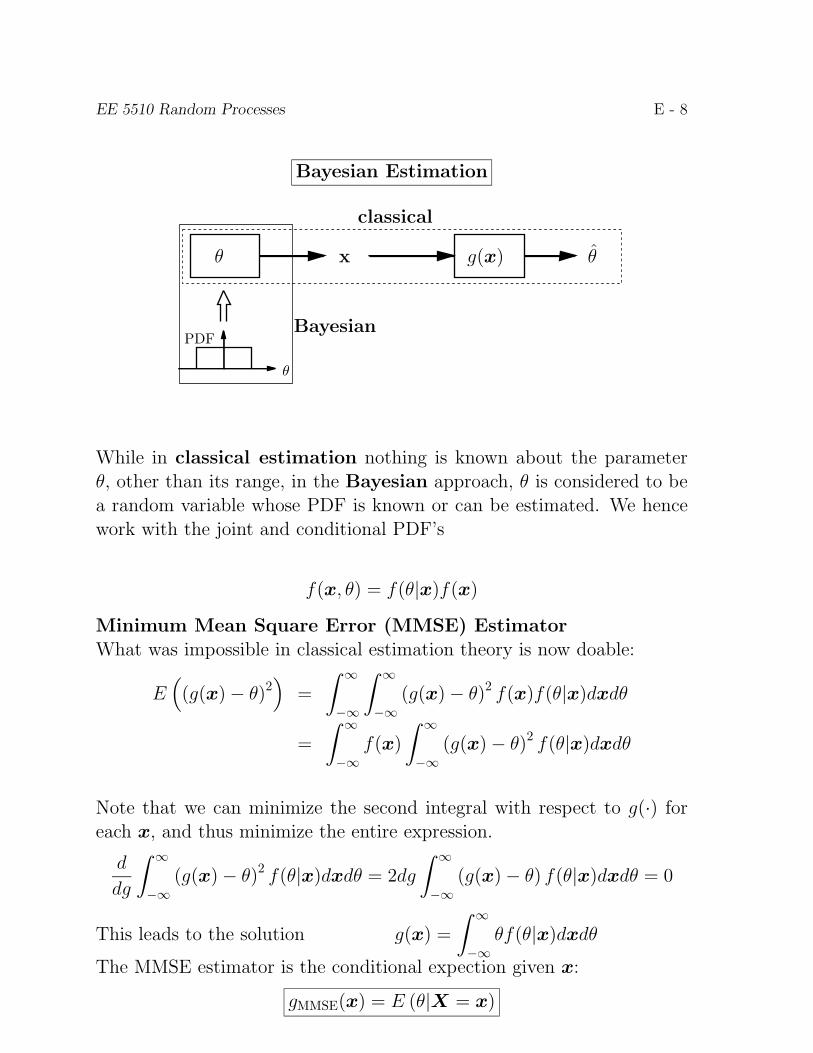
Bayesian Estimation

xθ

θ

θg(x)

PDF

classical

Bayesian

While in classical estimation nothing is known about the parameterθ, other than its range, in the Bayesian approach, θ is considered to bea random variable whose PDF is known or can be estimated. We hencework with the joint and conditional PDF’s

f(x, θ) = f(θ|x)f(x)

Minimum Mean Square Error (MMSE) EstimatorWhat was impossible in classical estimation theory is now doable:

E(

(g(x)− θ)2)

=

∫ ∞−∞

∫ ∞−∞

(g(x)− θ)2 f(x)f(θ|x)dxdθ

=

∫ ∞−∞

f(x)

∫ ∞−∞

(g(x)− θ)2 f(θ|x)dxdθ

Note that we can minimize the second integral with respect to g(·) foreach x, and thus minimize the entire expression.

d

dg

∫ ∞−∞

(g(x)− θ)2 f(θ|x)dxdθ = 2dg

∫ ∞−∞

(g(x)− θ) f(θ|x)dxdθ = 0

This leads to the solution g(x) =

∫ ∞−∞

θf(θ|x)dxdθ

The MMSE estimator is the conditional expection given x:

gMMSE(x) = E (θ|X = x)


Example: Consider again n observations of an amplitude A in Gaussiannoise, i.e.,

xi = A+ ni; 1 ≤ i ≤ n

The PDF of the observation vector x = (x1, · · · , xn) is nowinterpreted as a conditional probability density

fX |A(x|a) =1

(2πσ2)(n/2) exp

(− 1

2σ2

n∑i=1

(xi − a)2

)The critical assumption is now the PDF of A. We assume

fA(a) =1

(2πσ2A)(1/2) exp

(− 1

2σ2A

(a− µA)2)

We now need to calculate

A = E(A|x)

We use the following result: If x and y are jointly Gaussiandistributed, then

E(Y |x) = E(Y ) + CyxC−1xx (x− E(X))

Cy|x = Cyy − CyxC−1xxCxy

where

Cxx = E(XXT )− µxµTxCyy = E(Y Y T )− µyµTyCyx = E(Y XT )− µyµTx ; Cxy = CT

yx

Applying these formulas to our case with y = A we obtain

Cxx = σ2A11T + σ2I;Cyy = σ2

A;Cyx = σ2A1T


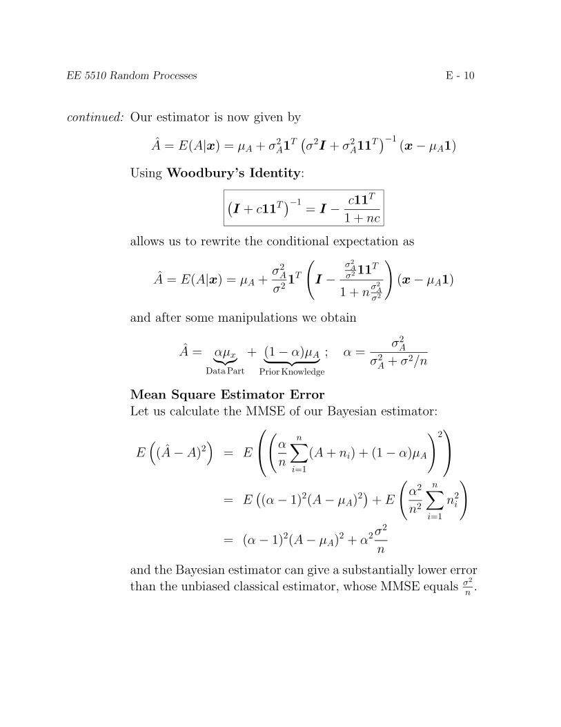
continued: Our estimator is now given by

A = E(A|x) = µA + σ2A1T

(σ2I + σ2

A11T)−1

(x− µA1)

Using Woodbury’s Identity:

(I + c11T

)−1= I − c11T

1 + nc

allows us to rewrite the conditional expectation as

A = E(A|x) = µA +σ2A

σ2 1T

(I −

σ2A

σ2 11T

1 + nσ2A

σ2

)(x− µA1)

and after some manipulations we obtain

A = αµx︸︷︷︸Data Part

+ (1− α)µA︸︷︷︸Prior Knowledge

; α =σ2A

σ2A + σ2/n

Mean Square Estimator ErrorLet us calculate the MMSE of our Bayesian estimator:

E(

(A− A)2)

= E

(αn

n∑i=1

(A+ ni) + (1− α)µA

)2

= E((α− 1)2(A− µA)2)+ E

(α2

n2

n∑i=1

n2i

)

= (α− 1)2(A− µA)2 + α2σ2

n

and the Bayesian estimator can give a substantially lower errorthan the unbiased classical estimator, whose MMSE equals σ2

n .


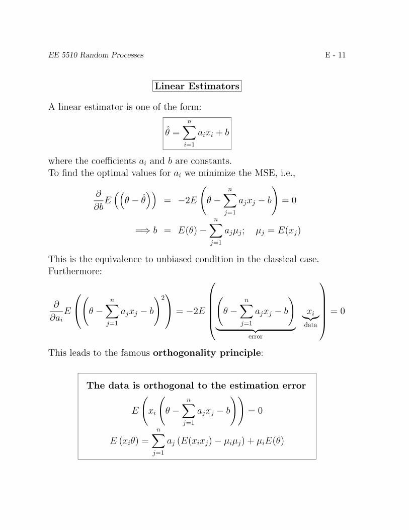
Linear Estimators

A linear estimator is one of the form:

θ =n∑i=1

aixi + b

where the coefficients ai and b are constants.To find the optimal values for ai we minimize the MSE, i.e.,

∂

∂bE((θ − θ

))= −2E

(θ −

n∑j=1

ajxj − b)

= 0

=⇒ b = E(θ)−n∑j=1

ajµj; µj = E(xj)

This is the equivalence to unbiased condition in the classical case.Furthermore:

∂

∂aiE

(θ − n∑j=1

ajxj − b)2 = −2E

(θ −

n∑j=1

ajxj − b)

︸︷︷︸error

xi︸︷︷︸data

= 0

This leads to the famous orthogonality principle:

The data is orthogonal to the estimation error

E

(xi

(θ −

n∑j=1

ajxj − b))

= 0

E (xiθ) =n∑j=1

aj (E(xixj)− µiµj) + µiE(θ)


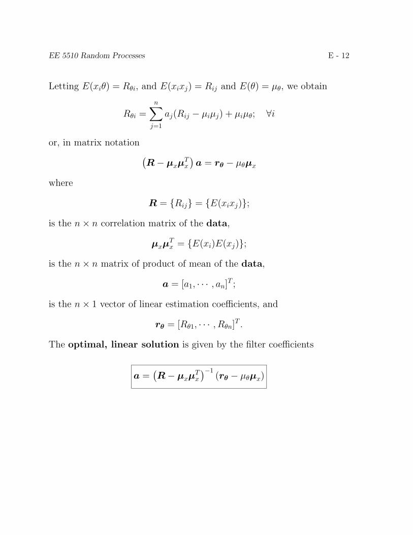
Letting E(xiθ) = Rθi, and E(xixj) = Rij and E(θ) = µθ, we obtain

Rθi =n∑j=1

aj(Rij − µiµj) + µiµθ; ∀i

or, in matrix notation (R− µxµTx

)a = rθ − µθµx

where

R = {Rij} = {E(xixj)};

is the n× n correlation matrix of the data,

µxµTx = {E(xi)E(xj)};

is the n× n matrix of product of mean of the data,

a = [a1, · · · , an]T ;

is the n× 1 vector of linear estimation coefficients, and

rθ = [Rθ1, · · · , Rθn]T .

The optimal, linear solution is given by the filter coefficients

a =(R− µxµTx

)−1(rθ − µθµx)


Linear Prediction

Consider a stationary discrete random process x = (x1, x2, x3 · · · ). Wewant to predict the value of xn+j, given the values up to xn, and let usassume that E(xi) = 0 for simplicity.

We will use a linear estimator, i.e., we let θ = xn+j and calculate

xn+j =N−1∑i=0

aixn−i

The parameter N is the predictor order, i.e., the number of previoussamples which are used to predict the new sample value.The solution is given by:

a = R−1r

where, since the process is stationary and Rij = Rj−i

r = [Rj+N−1, · · · , Rj]T

and

R =

R0 R1 · · · RN−1

R1 R0 · · · RN−2...

...RN−1 RN−2 · · · R0

These equations are known as the Yule-Walker prediction equations,or also as the Wiener-Hopf equations.


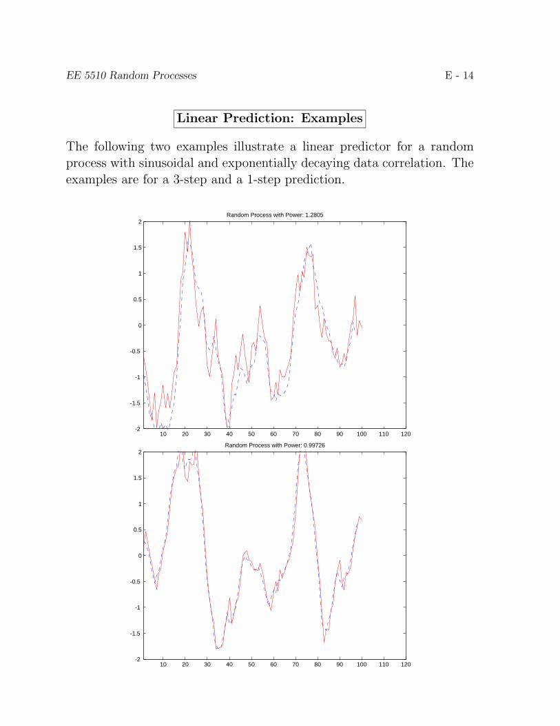
Linear Prediction: Examples

The following two examples illustrate a linear predictor for a randomprocess with sinusoidal and exponentially decaying data correlation. Theexamples are for a 3-step and a 1-step prediction.

10 20 30 40 50 60 70 80 90 100 110 120-2

-1.5

-1

-0.5

0

0.5

1

1.5

2Random Process with Power: 1.2805

10 20 30 40 50 60 70 80 90 100 110 120-2

-1.5

-1

-0.5

0

0.5

1

1.5

2Random Process with Power: 0.99726


Mean Square Error

E(

(xn+1 − xn+1)2)

= E(x2n+1)− 2E (xn+1xn+1) + E

(x2n+1)

Orthogonality:E((xn+1 − xn+1)xn+1) = 0E(xn+1xn+1) = E(x2

n+1)= σ2

x − E (xn+1xn+1)

= σ2x −

N−1∑i=0

aiE (xn+1xn−i)

= σ2x −

N−1∑i=0

aiRi+1

= σ2x − aTr = σ2

x − rTR−1r

These principles can be used for filtering, prediction or smoothing

Data

Data

Data

Smoothing:

Prediction:

Filtering:


Linear Estimation of Many Parameters

Let us assume that we want to estimate L parameters θl, where the l-thparameter is estimated via the linear equation:

θl =n∑i=1

alixi + bl = aTl x+ bl

• First we find the constant term bl via the MMSE principle:

∂

∂blE((

Θl − aTl X − bl)2)

= −2E(Θl − aTl X − bl

)= 0

and hence

bl = E (Θl)− aTl E (X)

• Second, we proceed to evaluate the values of the coefficients al

∂

∂aliE((

Θl − aTl (X − E(X))− E(Θl))2)

= −2E((

Θl − aTl (X − E(X))− E(Θl))

(Xi − E(Xi)))

= −2E ((Θl − E(Θl)) (Xi − E(Xi))− 2E(aTl (X − E(X)) (Xi − E(Xi))

)= −2Cθlxi − 2aTl Cxxi, ∀l, i

where

Cxxi = [E ((X1 − E(X1)(Xi − E(Xi)) , · · · , E((XL − E(XL)(Xi − E(Xi))]T ;

Collecting all i terms into a vector equation we obtain: Cθlx1

...Cθlxn

T = aTl [Cxx1, . . . , Cxxn]

CTθlx

= aTl Cxx


From this we obtain the optimal estimator coefficients:

aTl = CTθlxC−1xx

and we derive the estimator for θl as

θl = aTl (x− E(X)) + E(Θl) = CθlxC−1xx (X − E(X)) + E(Θl); ∀l

Summarizing the L equations above into a single matrix equation

θ = A (x− E(X)) + b = CθxC−1xx (x− E(X)) + E(Θ)

Note: This has exactly the same form as the conditional expectation forjointly Gaussian random vectors, see page E - 9, and hence θ is theoptimal estimator if θ and x are Gaussian distributed.

Note: This linear estimator uses only second order statistics, i.e.,

Cθx, Cxx, E(X), E(Θ)

Mean Square Error (MSE)The mean square error of the linear estimator can be calculated as

MSEθ

= E

((Θ− Θ

)(Θ− Θ

)T)= E

((Θ− E(Θ)− A(X − E(X)) (Θ− E(Θ)− A(X − E(X))T

)= Cθθ + ACxxA

T − ACxθ − CθxA

MSEθ

= Cθθ − CθxC−1xxCxθ


Channel EstimationConsider the unknown discrete channel shown below:

. . . . .

. . . . .h0wn

un

h1 h2 hp-1

xn

z-1 z-1 z-1

the output data is given by

x =

u0

u1 u0...

......

...uN−1 uN−2 · · · uN−p

h0

h1...

hp−1

+w = Uh+w

The data covariance matrix is given by:

Cxx = E((X − E(X))

(X − E(X)T

))= E

((U (H − µh)) (U (H − µh))T

)= HE

((H − µh)(H − µh)T

)HT + E

(wwT

)= UChhU

T + Cww

The optimal Bayesian estimator for this problem is given by:

h = ChhU(HChhU

T + Cww)−1

(x−Uµh)) + µh

If the taps are uncorrelated with zero mean: Chh = I,µh = 0, then

h = U(UUT + Cww

)−1x


MMSE Channel Estimator

The matrix UUT has rank at most n, and hence(UUT + Cww

)is only invertible is Cww is not (close to) zero. That is, the noise drivesthe estimator. In this case we apply the matrix inversion lemma:

(A+BCD)−1 = A−1 −A−1B(DA−1B +C−1)DA−1

to the required inverse with the identifications:

A = Cww

B = U

C = I

D = UT

This gives us, after some manipulations, and with Cww = σ2I:(UUT + Cww

)−1=

1

σ2

(I −U

(UUT + σ2IUT

))and, finally a simpler formula for the optimal channel estimates:

h =(UUT + σ2I

)−1UTx

Remarks: • The size of the inverse is now only p× p, a significant gainin simplicity

• Signal Design: If the probing signals are designed suchthat UUT ≈ nI, the inverse becomes trivial, and

h =1

n+ σ2UTx

In this case the error is also best, given by

MSEh

= Chh − ChxC−1xxCxh =

σ2/n

1 + σ2/nI


Wiener Filtering

Consider a system where a signal is observed in noise, i.e.,

x = θ +w = s+w

• parameters evolve continuously

• as many parameters as measurements

Using an optimal linear estimator we obtain the Wiener Filter for thisprocess:

s = Css (Css + Cww)−1 x

Note that the filter makes use of prior information in the form of thesignal correlation Css.Filter Interpretation

s = Css (Css + Cww)−1 x = Fx

This implies the time-varying filter:

sn =n∑k=0

f(n)n−kxk = f (n)Tx

sn = rTss (Css + Cww)−1 x

where

• rTss is the last row of Css

• f (n) = [f(n)n , · · · , f (n)

0 ] is the last row of F (note the inverse orderingof the subscripts)


The equations

(Css + Cww)f (n) = rss

are the well-known Wiener-Hopf equations (see E - 13):r0 + σ2 r1 · · · rnr1 r0 + σ2 · · · rn−1...

...rn − 1 rn−1 · · · r0 + σ2

f

(n)n

f(n)n−1...

f(n)0

=

rnrn−1

...r0

where rif is the (i, j)-th entry of Css, and Cww is diagonal.

Note: For large values of n the filter taps will become constant since rn →0 as n→∞:

r0 + σ2 · · · rp−1 0 · · · 0r1 r0 + σ2 · · · rp−1 0 0

. . .. . .

0 0 rp−1 · · · r0 + σ2

0 · · · 0 rp−1 · · · r0 + σ2

0...0

f(n)p−1...

f(n)0

=

0...0rp−1

...r0

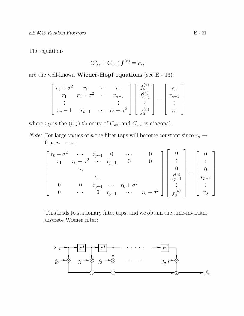
This leads to stationary filter taps, and we obtain the time-invariantdiscrete Wiener filter:

. . . . .

. . . . .f0

x� n

f1 f2 fp-1

sn

z-1 z-1 z-1

^

Estimation Theory Basics What is Estimation best something...

Documents

Transcript of Estimation Theory Basics What is Estimation best something...