Estimation of Water Quality Parameters for Lake Kemp Texas Derived From Remotely Sensed Data.

Bassil El-Masri and A. Faiz Rahman

Department of Natural Resources Management, Texas Tech University, Box 42125, Lubbock, TX 79409. Current address: Department of Geography, Indiana University, 701 E. Kirkwood Ave., Bloomington, IN 47405. Corresponding author email: belmasri@indiana.edu

Abstract:

Remote sensing of water quality would provide resource managers’ with tools to monitor and maintain water bodies in a well-timed and cost-effective manner. The primary aim of this study was to estimate chlorophyll a, total phosphorus (TP), and turbidity using remote sensing data derived from the Moderate Resolution Imaging Spectrometer (MODIS). Based on in situ measurements from Lake Kemp collected in June and October of 2006, and MODIS reflectance data acquired for the same time period, spectral indicators for the above mentioned water quality parameters were calculated. Chlorophyll a and TP concentrations were quantified using the ratios of (MOD1- MOD14)/(MOD14 + MOD2) and MOD12/MOD13, respectively, which showed a linear relationship with in-situ data. Turbidity was quantified using the ratio of (MOD2 – MOD4)/( MOD11 × MOD12). Chlorophyll a and turbidity had the strongest correlation (r2 = 0.81, r2 = 0.92 respectively) with in situ measurements, while TP had the lowest correlation (r2 = 0.56). Maps for chlorophyll a distribution as well as for TP and turbidity were generated from MODIS data.

Keywords: Chlorophyll a; turbidity; total phosphorus; remote sensing. Introduction

Inland water bodies are considered important ecological and sociological zones. Many lakes (natural and man-made) and rivers are the main sources for drinking water as well as for agricultural usage. According to Brooks et al. (2003) water quality standard refers to the physical, chemical, or biological characteristics of water in relation to a specific use.

Protection and maintenance of water quality is a primary objective for watershed or resource managers. Increase of chlorophyll a, turbidity, total suspended solids (TSS) and nutrients in lakes are symptomatic of eutrophic conditions (Shafique et al. 2002). Sediments also affect water quality and thus its suitability for drinking, recreation and other activities. It serves as a carrier and storage agent for nitrogen, phosphors and organic compounds that can be indicators of pollution (Jensen 2000).

The traditional measurement of water quality requires in situ sampling, which is a costly and time-consuming effort. Because of these limitations, it is impractical to cover the whole water body or obtain frequent repeat sampling at a site. This difficulty in achieving successive water quality sampling becomes a barrier to water quality monitoring and forecasting (Senay et al. 2001). It would be advantageous to watershed managers to be able to detect, maintain and improve water quality conditions at multiple river and lake sites without being dependent on field measurements (Shafique et al., 2002).

Remote sensing techniques has the potential to overcome these limitations by providing an alternative means of studying and monitoring water quality over a wide range of both temporal and spatial scales (Senay et al., 2001). Several studies have confirmed that remote sensing can meet the demand for the large sample sizes required for water quality studies conducted on the watershed scale (Senay et al., 2001). Hence, it is not surprising that a significant amount of research has been conducted to develop remote sensing methods and indices that can aid in obtaining reliable estimates of these important hydrological variables. These methods ranged from semi-empirical techniques to analytical methods for estimating and producing quantitative water quality maps (Dekker 1997 cited in Shafique et al., 2002). Several researchers (Gitelson et al., 1992, Dekker et al., 1996, Dekker et al., 2002) have developed different models to predict several lake water quality parameters from satellite data by employing spectral ratios or indices. These water quality parameters have included chlorophyll a concentration, suspended matter concentrations and turbidity.

1

In nature the upwelling radiance from lakes or rivers is the combination of all the constituents of the water column, that includes suspended organic, inorganic, and pigment (Han and Rundquist, 1997). The bottom of the shallow water can also contribute to the radiance leaving the water. Hence, determining which signal is attributable to a particular water quality parameter is not an easy task (Han and Rundquist, 1997). In general, the optics of water–sediment mixtures are highly nonlinear, while many factors such as suspended particle size, shape and color can have large influences on water–sediment optics (Warrick et al., 2004). Due to these optical complexities it is well known that there are no universal algorithms to remotely estimate sensed sediment concentrations (Warrick et al., 2004).

However, differentiating the influence of suspended sediment concentrations (SSC) and chlorophyll a on spectral reflectance characteristics when using coarse spectral resolution imagery such as Landsat Thematic Mapper (TM) and Enhanced Thematic Mapper Plus (ETM+) remains problematic (Svab et al., 2005). Lindell et al. (1999) concluded that chlorophyll a determination is not possible when SSC increases and is heterogeneously distributed.

Tyler et al (2006) used a mixed model to derive chlorophyll a concentration in lakes using Landsat TM images. Linear regression models were developed to estimate total suspended matter concentrations using Landsat TM data (Zhou et al., 2006). In addition, Svab et al. (2005) concluded that spectral mixture modeling can be used to estimate chlorophyll a concentration in water with high heterogeneous SSC distribution.

The purpose of this study was to estimate chlorophyll a concentration, total Phosphorus concentration, and turbidity using spectral indices. First, spectral indices developed by Shafique et al, 2002 for hyperspectral data were modified in order to make them suitable for use with multispectral remote sensing, specifically the Moderate Resolution Imaging spectrometer (MODIS) onboard NASA’s ‘Terra’ and ‘Aqua’ Earth observation satellites. We tested these modified indices to Lake Kemp, Texas. The second step included determination of the optical properties of the water parameters mentioned above and selection of spectral bands that are used in the indices in order to develop spectral indices using MODIS data. Remote sensing data were validated with field measurement to test the accuracy of the indices. The final objective was to present and provide sequential and spatial images of water quality estimates to provide decision makers with easily applicable information.

Materials and Methodology Study area

Lake Kemp is located on Wichita River north of Seymour in Baylor County, Texas (Fig.1). It covers an area of 15,590 acres with a maximum depth of 53 feet, has a depth fluctuation of 6-8 feet annually and 4-6 feet depth visibility. The annual precipitation is 24 inches/year, average temperature is 63o F and the elevation is 1,114 ft above mean sea level.

Data

We utilized MODIS imagery from May 2001 to December 2001, covering two periods of the dry and wet seasons for Lake Kemp, for our initial model development. Based on previous studies and spectral analysis, nine MODIS reflectance bands were used in this study. Concurrent limnological data, collected by Wilde (2003) was used. These limnological data include chlorophyll a, total phosphorus and turbidity measurements collected from Lake Kemp during 2001-2002. MODIS data were available on a daily basis, and free for research use. After the initial development of spectral reflectance vs. limnological parameters’ relationships, we collected data and MODIS images in June and October of 2006 to validate and refine our models. Five samples with three replications were collected from the lake during that period.

Laboratory analysis Chlorophyll a from water samples was extracted in 100 percent acetone the day following the samples collection. Spectral absorption measurements for chlorophyll a were carried out the day after the extraction was done with spectrophotometer using wavelength 661.6nm and 644.8nm as suggested by Lichtenthaler, 1987. The concentration for chlorophyll a (unit = ug/l) was quantified using the equations adopted from Lichtenthaler, 1987. On the other hand, turbidity is usually measured in Nephelometric Turbidity Units (NTU) that refers to the way the instrument, a

2

nephelometer, measures how much light is scattered by suspended particles in the water. Turbidity and TP (unit = mg/l) were analyzed in a private lab following the methods recommended in Standard Methods for the Examination of Water and Wastewater 20th edition and EPA SW-846 respectively. Criteria of MODIS Band Selection

The reflectance of a water body depends upon absorption and scattering of incoming radiation. This absorption and scattering is a function of the material present in the surface water (Senay et al., 2001). According to Jenson (2000), visible wavelengths between 580 – 690 nm may provide information on the type of suspended sediment in the surface water, while the near-infra red wavelength range of 714 – 880 nm can be useful for determining the amount of these materials. In addition, Gitelson (1992) and Rundquist et al. (1995) found that strong chlorophyll a absorption of red light is approximately at 675nm and the predominant reflectance peak is around 690 – 700nm. Thus the height of this peak above the baseline (670 – 750nm) can be used to measure chlorophyll amount (Rundquist et al., 1995).

Mittenzwey et al. (1992) found a high coefficient of determination (r2) of 0.98 between chlorophyll a and the near-infrared (NIR)/red reflectance ratio (cited in Han and Rundquist, 1997). Han and Rundquist (1997) and Rundquist et al. (1996) estimated the chlorophyll a pigment amount in surface water using the ratio of near-infra red (705nm)/red (670nm) ratio when the concentration was low. On the other hand, the best result was derived from reflectance around 690nm when chlorophyll a concentration was high. Regions of the spectrum at wavelengths near 450-550nm, 675-750nm and 800-1000nm were found to be good estimators of turbidity (Senay et al., 2001).

Model Development

Based on these above-mentioned assumptions, this study proposed modification of water quality indices developed using hyperspectral remote sensing by Shafique et al., (2002) to make them useable with multispectral sensors. The indices proposed by Shafique et al., (2002) were:

876.34)(849.48 675705 −÷= RRalChlorophyl

0371.0)log(18081.0)( 675554 −÷×= RRTPPhosphorusTotal

5516.8)(59.186 740710 +−= RRTurbidity

(1)

(2)

(3)

where R is the reflectance at the spectral wavelength (nm) expressed by the subscript number. We used reflectance values of MODIS bands #13 (662 – 672nm) and #14 (673 – 683nm) to

estimate chlorophyll a concentration, #15 (743 – 753nm) and #16 (862- 877nm) to estimate turbidity, and #14 (673 – 683nm) and #12 (546 – 556nm) to estimate total phosphors (TP). Hence, the water quality indices modified for MODIS bands were proposed as:

876.34)1314(849.48 −÷= bbalChlorophyl 0371.0)1412log(18081.0)( −÷×= bbTPPhosphorusTotal

5516.8)1516(59.186 +−= bbTurbidity

(4)

(5)

(6)

where b and the subsequent numerals stand for MODIS band numbers. Chlorophyll a, turbidity and total phosphorus were calculated using the indices 4, 5 and 6 and

then correlated with the data collected in 2001.This analysis was performed in order to examine their capability to estimate water quality parameters using MODIS data. Low correlation between the indices 4, 5 and 6 and MODIS data was detected. The analysis of this correlation was the first step in the process to develop new indices and to validate them using the data collected in 2006.

Single spectral bands, ratios of bands, and combination of multiple bands were used to develop the indices. Scatter plots were created between spectral bands and ground truth data and spectral bands of interest against each other. Simple linear regression was used to determine the relationship between single and combinations of bands and water quality parameters. Then, the entire images were converted to water quality maps based on the indices developed.

MODIS reflectance bands 1 to 16 were used to test for relationship with water quality parameters to determine which bands and parameters correlated the most with better certainty. Scatter plots showed that the ratio of (b2 – b4)/ (b11 × b12) and (b1 – b14)/ (b14 + b2) can be used to estimate turbidity and chlorophyll a respectively. The ratio of b12/b13 was the best indicator for total Phosphorus. Also, it was found that MODIS b13 and b4 correlated strongly (r2 = 0.76). In the case

3

where no data were available for b13 such as for June 2006, b4 was used instead. Hence, the new indices developed for this study were:

( )[ ] ( )214/141 bbbbABSalChlorophyl +−= 13/12)( bbTPPhosphorusTotal =

( )[ ] ( )1211/42 bbbbABSTurbidity ×−=

(7)

(8)

(9)

where ABS[] indicates the absolute value.

Results and Discussion The evaluation of the band selection criteria led to the selection of particular bands that were

used to developed spectral indices for the estimation of the desired water quality parameters. The correlation between MODIS developed indices and ground measurements varied between water quality parameters and seasons.

The values for the water quality parameters were higher in the dry season (October) compared to the wet season (June). Chlorophyll a was stable between the two seasons (mainly higher values in October) ranging from 6 - 10 ug/l, whereas turbidity showed huge variation from a mean of 0.114 NTU in June to 23.46 NTU in October. This variation was coupled with increase in TP variation and values from a mean of 0.05 mg/l in June to a mean of 0.06 mg/l in October.

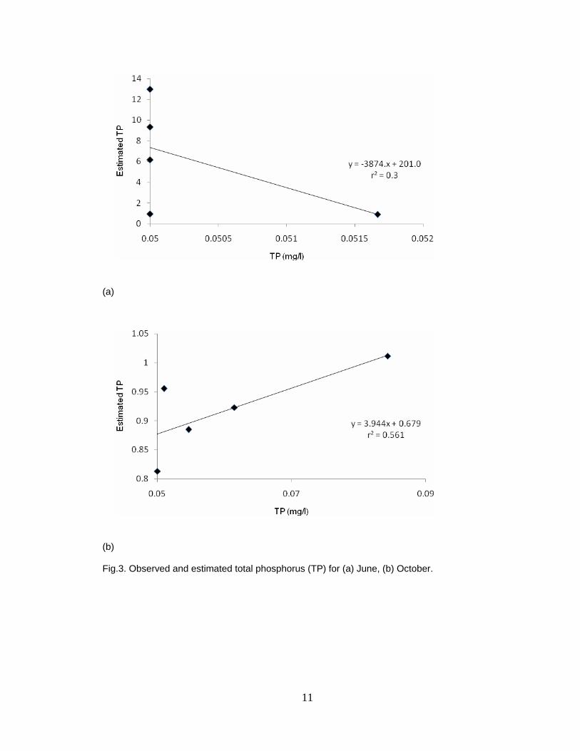
The ratio of bands 1, 2, and 14 as shown in equation 7 produced a good correlation (r2= 0.82) with chlorophyll a concentration in October 2006 (Fig.2). Where as, a week correlation (r2= 0.3) was observed between the same index and chlorophyll a concentration in June 2006 (Fig.2). Turbidity and the ratio of bands 2, 4, 11, and 12 (equation 8) correlated strongly (r2 = 0.92 and r2 = 0.79) for both June and October 2006 respectively (Fig.3). The ratios of b12 and b13 had a good correlation (r2 = 0.56) with TP in October of 2006, while the correlation was week (r2 = 0.3) for June 2006 (Fig.4). Thus, TP had the weakest correlation with MODIS bands.

The MODIS images were transformed to water quality parameters maps by using the indices developed. This was done pixel by pixel through the development of modules using ERDAS Imagine software. The results were six maps for chlorophyll a, turbidity, and TP for both June and October. The spatial distributions of chlorophyll a showed variation between the wet and the dry seasons. The highest values can be observed on the north to north east of the lake (Fig.4 and Fig.5).

Meanwhile, Turbidity and TP had many pixels of missing data for the lake in June and October. TP spatial distribution (June) was some how similar through out the lake with the highest values in the northwest of the lake (Fig. 6). This spatial distribution for TP can be detected in October especially in the west parts of the lake, in spite of the large number of missing data (Fig.7). On the other hand, the spatial distribution for turbidity showed a significant variation between June and October (Fig.8 and Fig.9). Moreover, the spatial variation within the lake was more obvious in October compared to June (Fig.8 and Fig.9). Turbidity was higher in the west and south of the lake compared to the north and east parts of the lake (Fig.8 and Fig.9).

Lake Kemp experienced enormous fluctuation in water level during the study period, especially in the east part of the lake. On October 15, Lake Kemp received 82.5 mm of rainfall in one event (data from Lake Kemp weather station available on NOAA website: http://cdo.ncdc.noaa.gov/pls/plclimprod/poemain.accessrouter?datasetabbv=SOD&countryabbv=&georegionabbv=&forceoutside= ) which is about one week prior to the samples collection. Regardless of that, the water level in the lake was extremely low where the east part of the lake was approximately dry.

Our results revealed that there was an increase in turbidity values from June to October, which can be related to the extreme rainfall event mentioned above. Also, this sudden increase can be associated with high erosion event that characterized Wichita River drainage (Lake Kemp is a moderately large impoundment of Wichita River) (Greiner 1982, cited in Wilde, 2003). Most of the erosion (71%) in the basin is sheet and rill erosion, both of which are associated with overland runoff following rain events (Wilde, 2003). Over land flow caused by rainfall is considered one of the non- point sources that cause turbidity to increase (Senay et al., 2001). On the other hand, chlorophyll a and TP concentration were similar in both the dry and the wet season.

Apparently, the variation within the lake in water quality parameters values might have an effect on the correlation between those parameters and the indicators developed from MODIS data. This is

4

noticeable through the comparison of the correlations for both June and October. The result for the data collected for TP in June were constant across the lake (0.05 mg/l), in which 4 out of the 5 samples collected had the same value The negative and week correlation between TP and equation 8 in June might be related to the fact that band 13 was replaced by band 4 and to the little, even no, variation in the TP sampling results as mentioned above. Another reason could be related to sampling size limitations where 5 samples might not be enough to detect changes in Lake Kemp TP during the period where there is a little variation in TP values.

To examine the effect of the sampling size we joined the data for both June and October together, so we had 10 samples instead of 5, only turbidity (equation 9) showed a good correlation with r2 = 0.55 (results not shown). Also, we average chlorophyll a, TP and turbidity data as well as MODIS bands values for both June and October, in this case only chlorophyll a (equation 7) showed very strong correlation with r2 = 0.83 (results not shown). It could be noticed that this attempt to increase the sample size is not adequate enough to detect the sampling size effect on the correlations obtained from the above equations. By averaging the MODIS pixel values for the study period that might have minimized any uncertainties in the values and the same is true for the measured chlorophyll a data. This led to a strong correlation and to the assumption that chlorophyll a could be better detected annually than seasonally using remotely sensed data.

We also regressed the field data for chlorophyll a, TP and turbidity against each other to inspect the relationship between them. This was not done for TP June data since TP values were similar to each other. Only turbidity and TP showed a good correlation and a little variation in the coefficient of determination was detected between October, the joined data for June and October and the average data where r2 ranged from 0.57 to 0.61 (results not shown). Based on that, a two-step procedure could be applied where TP can be estimated from the predicted turbidity. Therefore, an indirect approach can be used to estimate water quality parameters from spectral data when a week correlation exists between them.

In general, our chlorophyll a sampling results were less than 10mg/l. Several studies found that the largest relative errors in chlorophyll a prediction were for values less than 10 mg/l (Dall’Olmo and Gitelson, 2004 and Gons et al., 2002). One of the main reasons is that the chlorophyll a specific absorption coefficient near the chlorophyll a red-absorption maximum showed its maximum variability for chlorophyll a below 10mg/l (Dall’Olmo and Gitelson, 2004). This might have contributed to the week correlation between chlorophyll a and the MODIS data for June. Moreover, there was a little variation in the chlorophyll a ground data in June compared to October and that might also caused this week correlation. Regardless of that, our methodology showed that it has the ability to predict chlorophyll a even when it is present in the lake in low values. Also, this reveals the ability for our methodology that is based on MODIS data to detect variation in water quality parameters during the period when there exist variations within those parameters across the lake.

Mapping the water quality spectral indices revealed the ability of these indices to detect spatial and temporal variation in chlorophyll a, turbidity, and TP. For instance, higher values of turbidity can be observed beside the lakeshores, especially the south part, where most of the residential areas are located and the west side where Wichita River enters the lake. The higher values for chlorophyll a in the west and north parts of the lake can be related to the presence of aquatic plants. In addition, the spatial distribution for the calculated turbidity has east to west gradient that is consistent with the results for Lake Kemp limnological report by Wilde, 2003.

Conclusion

The study demonstrated a procedure for estimating and mapping specific water quality parameters for inland water using MODIS data. This was done through the development of water quality spectral indices and applying them to the MODIS data. Based on this study, we think chlorophyll a, turbidity, and TP of lake Kemp can be estimated and mapped using MODIS data. These methods may also be applied to estimate water quality parameters for other inland water bodies. Our results indicated that chlorophyll a (more than turbidity or TP) has a unique spectral signature that makes it possible to develop spectral indices to estimate its concentrations in lakes. One of the limitations we faced was the missing pixels values specifically for MODIS band 13 that might have an effect on the analysis of TP in June. Another problem was the similar and low TP sampling values across the lake which makes it difficult to develop an index to predict TP. Also,

5

further investigation is needed to test the accuracy of the approach presented in this paper using larger sample size.

Mapping the spatial distribution for chlorophyll a, turbidity, and TP with remotely sensed data would be helpful for management of water bodies by determining the point and non point sources that are responsible for such spatial variability. Thus, we conclude that remote sensing can potentially be used as a tool for monitoring water quality throughout the seasons and can provide natural resource managers and decision makers with crucial information. Future research should focus more on the use of remotely sensed data to estimate seasonal variations in water quality parameters.

Acknowledgment

This work was supported by a grant from USGS through TWRI. We want to thank Texas Tech University department of Natural Resources Management for the support for this study. We would like to show our appreciation to Tamara Enriquez, Vicente Cordova for their help in the field data collection. We want to thank John and Rollin Garrett for their assistant during the field work. Also we would like to thank Dr. Scott Holaday for his help and offering his lap to us for chlorophyll a analysis. Finally, we would like to thank Dr. Gene Wilde for allowing us to use his data. References Brooks, K.N., Ffolliott, P.F., Gregersen, H.M., and DeBano, L.F 2003. Hydrology and the

Management of Watersheds. Third Edition. Iowa State University Press/ Ames. Dekker, A.G., Zamurovic-Nenad, Z., Hoogenboon, H., J., and Peters, S. W. M., 1996. Remote Sensing, ecological water quality modelling and in situ measurements: a case study in shallow lakes. Hydrological Sciences. 41(4): 531 – 547.

Dekker, A.G., Vos, R., J., and Peters, S., W., M., 2002. Analytical algorithms for lake water TSM estimation for retrospective analysis of TM and SPOT sensor data. International Journal of Remote Sensing. 23(1): 15 – 35.

Dall’Olmo, G. and Gitelson, A.A., 2005. Effect of bio-optical parameter variability on the remote estimation of chlorophyll-a concentration in turbid productive water: experimental results.

Applies Optics. 44(3): 412 - 422 Gitelson, A.A. 1992. The Peak Near 700nm on Radiance Spectra of Algae and Water:

Relationships of its Magnitude and Position with Chlorophyll a concentration. International Journal of Remote Sensing.13: 3367 – 3373.

Gons, H.J., Rijkeboer, M. and Ruddick, K.G., 2002. A chlorophyll-retrieval algorithm for satellite Imagery (Medium Resolution Imaging Spectrometer) of inland and coastal water. Journal of Plankton Research. 24: 947 – 951.

Han, L., and Rundquist, D.C., 1997. Comparison of NIR/RED Ratio and First Derivative of Reflectance in Estimating Algal- Chlorophyll Concentration: A Case Study in a Turbid Reservoir. Remote Sensing of Environment. 62: 253 – 261.

Jensen, J.R. 2000. Remote Sensing of the Environment: An Earth Resource Prospective. Prentice Hall Series in Geographic Information System.

Lichtenthaler, H.K., 1987. Chlorophylls and carotenoids: Pigments of photosynthetic biomembranes. Methods in Enzymology. 148: 350 – 382. Rundquist, D.C., Schalles, J.F., and Peake, J.S., 1995. The Response of Volume Reflectance to

Manipulated Algal Concentrations above Bright and Dark Bottoms at Various Depths in an Experimental Pool. Geocarto International. 10: 5 -14.

Rundquist, D.C., Han, L., Schalles, J.F., and Peake, J.S., 1996. Remote Measurement of Algal Chlorophyll in Surface Waters: The Case for the First Derivative of Reflectance Near 69nm. Photogrammetric Engineering and Remote Sensing. 62: 195 – 200.

Shafique, N.A., Fulk, F., Autrey, B.C., and Flotemersch, J. 2002. Hyperspectral Remote Sensing of Water Quality Parameters for Large Rivers in the Ohio River Basin. Available at: http://www.tucson.ars.ag.gov/icrw/Proceedings/Shafique.pdf.

Senay, G.B., Shafique, N.A., Autrey, B.C., Fulk, F., and Cormier, S.M., 2001. The Selection of Narrow Wavebands for Optimizing Water Quality Monitoring on the Great Miami River, Ohio using Hyperspectral Remote Sensor Data. J. of Spatial Hydrology. 1: 1- 22.

6

Svab, E., Tyler, A.N., Preston, T., Presing, M., and Balogh, K.V., 2005. Characterizing the spectral reflectance of algae in lake waters with high suspended sediment concentrations. International Journal of Remote Sensing. 26: 919 – 928.

Tyler, A.N., Svab, E., Preston, T., Presing, M., and Kovacs, W.A., 2006. Remote sensing of the water quality of shallow lakes: A mixture modeling approach to quantifying phytoplankton in water characterized by high suspended sediment. International Journal of Remote Sensing. 27: 1521 – 1537.

Warrick, J.A., Mertes, L.A.K., Siegel, D.E., and Mackenzie, C., 2004. Estimating suspended sediment concentrations in turbid coastal waters of Santa Barbara Channel with SeaWiFS. International Journal of Remote Sensing. 25: 1195 – 2002.

Wilde, G.R., 2003. Limnological survey of Lake Kemp, Texas: 2001. Submitted to U.S. Corps of Engineers, Tulsa district.

Zhou, W., Wang, S., Zhou, Y., and Troy, A., 2006. Mapping the concentrations of total suspended matter in Lake Taihu, China, using Landsat-5 TM data. International Journal of Remote Sensing. 27: 1177 – 1191.

7

Fig.1. Map of the Lake Kemp, Baylor County, Texas showing where the samples were collected. The red circles represent samples that were collected in June. The triangles represent samples collected in June and October. The stars represent samples collected in October.

8

(a)

(b) Fig.2. Observed and estimated chlorophyll a for (a) June , (b) October.

9

(a)

(b) Fig.3. Observed and estimated turbidity for (a) June, (b) October.

10

(a)

(b) Fig.3. Observed and estimated total phosphorus (TP) for (a) June, (b) October.

11

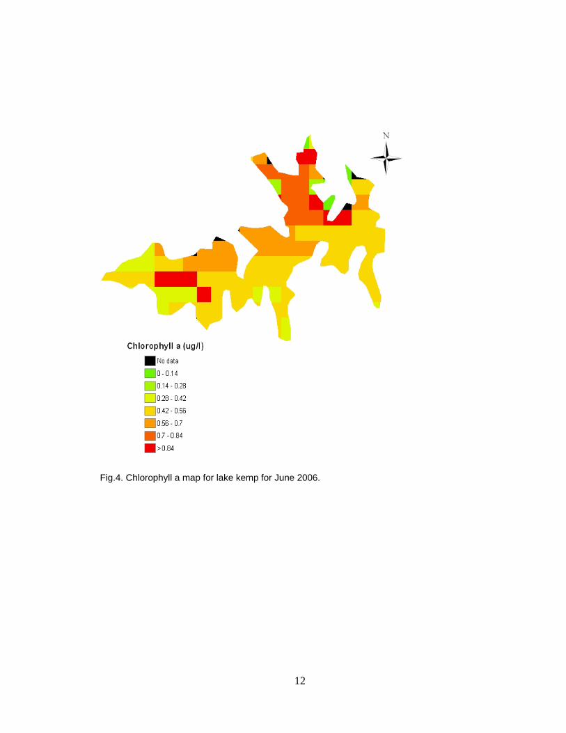
Fig.4. Chlorophyll a map for lake kemp for June 2006.

12

Fig.5. Chlorophyll a map for Lake Kemp for October 2006.

13

Fig.6. Total Phosphorus (TP) map for Lake Kemp for June 2006.

14

Fig.7. Total Phorsphorus (TP) map for Lake kemp for October 2006.

15

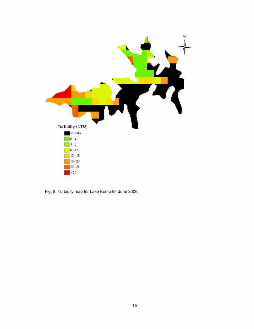
Fig. 8. Turbidity map for Lake Kemp for June 2006.

16

Fig.9. Turbidity map for Lake Kemp for October 2006.

17