Estimation of stochastic volatility models by nonparametric filtering

Shin Kanaya Dennis Kristensen

The Institute for Fiscal Studies Department of Economics, UCL

cemmap working paper CWP09/15

Estimation of Stochastic Volatility Models by

Nonparametric Filtering∗

Shin Kanaya†

University of Aarhus and CREATESDennis Kristensen‡

UCL, IFS and CREATES

March 2015

∗The authors wish to thank Bruce Hansen, Bent Nielsen, Neil Shephard, Yoshinori Kawasaki, Kotaro Hitomi,

Yoshihiko Nishiyama, Russell Davidson, Howell Tong, Pascale Valery and Karim Abadir for fruitful discussions and

helpful suggestions. They also wish to thank participants at seminars at University of Wisconsin-Madison, the

CREATES opening Conference, the 2007 EC2 Meeting, the 2009 Japanese Statistical Society Spring Meeting, the

4th London and Oxbridge Time Series Workshop, the 43rd Annual Conference of the Canadian Economics, the 2009

North American Summer Meeting of the Econometric Society, and the 2009 Far East and South Asia Meeting of

the Econometric Society for comments and suggestions. They also gratefully acknowledge support from CREATES,

Center for Research in Econometric Analysis of Time Series, funded by the Danish National Research Foundation

(DNRF78). Kristensen gratefully acknowledges financial support from the National Science Foundation (grant no.

SES-0961596). Part of this research was conducted while Kanaya was visiting the Institute of Statistical Mathematics

and the Institute of Economic Research at Kyoto University (under the Joint Research Program of the KIER),

and Kristensen was visiting Princeton University and University of Copenhagen, whose support and hospitality are

gratefully acknowledged.†Department of Economics and Business, University of Aarhus, Fuglesangs Alle 4, Aarhus V, 8210, Denmark.

E-mail: skanaya@econ.au.dk.‡Department of Economics, University College London, Gower Street, London, WC1E 6BT, United Kingdom.

E-mail: d.kristensen@ucl.ac.uk.

1

Proposed running head: Estimation of SV Models

Corresponding author:

Dennis Kristensen

Department of Economics

University College London

Gower Street

London WC1E 6BT

United Kingdom

E-mail: d.kristensen@ucl.ac.uk

Abstract: A two-step estimation method of stochastic volatility models is proposed. In the first

step, we nonparametrically estimate the (unobserved) instantaneous volatility process. In the

second step, standard estimation methods for fully observed diffusion processes are employed, but

with the filtered/estimated volatility process replacing the latent process. Our estimation strategy is

applicable to both parametric and nonparametric stochastic volatility models, and can handle both

jumps and market microstructure noise. The resulting estimators of the stochastic volatility model

will carry additional biases and variances due to the first-step estimation, but under regularity

conditions we show that these vanish asymptotically and our estimators inherit the asymptotic

properties of the infeasible estimators based on observations of the volatility process. A simulation

study examines the finite-sample properties of the proposed estimators.

Keywords: Realized spot volatility; stochastic volatility; kernel estimation; nonparametric; semi-

parametric.

JEL codes: C14; C32; C58.

2

1 Introduction

We propose a general estimation strategy for SV jump-diffusion models that combines a simple,

model-free realized volatility estimator with the additional structure imposed by the Markov diffu-

sion model of the volatility process. The resulting estimators are simple to implement and require

little, if any, numerical optimization. The estimation strategy allows for both nonparametric and

fully parametric specifications of the SV model, and as such is very flexible. The estimation method

proceeds in two steps: First, a nonparametric estimator of the spot (or instantaneous) volatility is

computed. Second, the spot volatility estimator is plugged into a given existing estimation method

for fully observed diffusion models.

The first step takes as input a given spot volatility estimator: A number of spot volatility es-

timators have been proposed in the literature such as Fan and Wang (2008), Kristensen (2010a),

Hoffman, Munk and Schmidt-Hieber (2012), Malliavin and Mancino (2002, 2009), Mancini, Mat-

tiussi and Renò (2012), and Zu and Boswijk (2014), amongst others. We do not restrict ourselves

to a specific volatility estimator, and allow for a broad class of spot volatility estimators to be

employed in our two-step procedure. In the second step, the volatility model is estimated taking

as input the chosen spot volatility estimator. We here consider two leading volatility models with

associated estimators: First, we consider a nonparametric Markov model for the volatility with

associated kernel estimators as proposed by Bandi and Phillips (2003). As a second example, we

analyze (semi-) parametric Markov models with associated least-squares estimators akin to the

ones proposed in Prakasa Rao (1988) or Bandi and Phillips (2007). The asymptotic theory that

we develop assumes that the volatility process contains no jump component. However, we show

how the estimators can be modified to handle jumps in volatility and discuss how our theory can

be extended to cover this case.

We show consistency and asymptotic normality for both the nonparametric and parametric

two-step estimators of the underlying volatility model. In the nonparametric case, our two-stage

estimation problem is similar to the one considered in Sperlich (2009) where kernel regression with

generated regressors is considered; see also Newey, Powell and Vella (1999), Xiao, Linton, Carroll

and Mammen (2003) and Mammen, Rothe and Schienle (2012). The parametric estimators can

be seen as a two-step semiparametric estimation procedure, where a parametric estimator relies

on a preliminary nonparametric estimator; see e.g. Kristensen (2010b) and Mammen, Rothe and

Schienle (2013).

The asymptotic properties of the two-step estimators are established under regularity conditions

with a key condition being that the first-step spot volatility estimator is uniformly consistent over

a growing time span with a known convergence rate. This is a high-level assumption that needs to

be verified for the particular spot volatility estimator being employed. We verify this condition for

three particular spot volatility estimators that are consistent under different scenarios as described

below. In all three cases, the proof of uniform consistency is technically demanding due to two

properties of the object of interest, the realized sample path of the latent volatility process: First,

it is not smooth, and second it is potentially unbounded as time diverges. This is in contrast to

3

standard nonparametric estimation problems (e.g. density and regression estimation), and we have

to use some novel theoretical techniques in order to establish uniform rate results over an expanding

time interval, including a new result on the global modulus of continuity of stochastic processes.

Four scenarios are considered in the first-step spot volatility estimation: First, the ideal situation

where log-prices are observed without market microstructure noise and do not contain jumps. In

this case, the kernel-based estimator proposed in Kristensen (2010a) is consistent, and we extend

Kristensen’s rate results to allow for an expanding time span. Second, noise is introduced and we

propose a novel spot volatility estimator based on pre-averaging, similar to Podolskij and Vetter

(2009a,b), to handle this case, and derive its uniform rate. Next, we consider the case where jumps,

but no noise, are present, and we derive the rate of a kernel-weighted version of the threshold

estimator of Mancini (2009). Finally, by combining the estimation strategies from the second and

third scenario, we develop a jump and noise-robust spot volatility estimator; the analysis of this

estimator proves to be quite complex, and so we do not provide a complete asymptotic theory for

this. The estimators in the second and fourth scenarios are both novel, and the uniform rate results

of all estimators are new contributions to the literature, and so should be of independent interest.

Our estimators rely on certain nuisance parameters that need to be chosen in the implemen-

tation. In particular, bandwidths have to be chosen in the estimation of the spot volatility. Our

theoretical results offer some guidance regarding how this and other parameters should be chosen.

Based on these, we discuss in some detail how the estimators can be implemented in practice. We

also investigate the finite-sample performance of our estimators through a simulation study with

particular emphasis on their sensitivity towards the choice of nuisance parameters. We find that

the estimators are quite robust and fairly precise for reasonable sample sizes.

Within the class of parametric Markov SV models, a number of different estimation methods

exist. If only low-frequency data is available, the estimation problem is hard due to the volatility

process being latent. In a few specific examples, one can derive analytical expressions of certain

moment functions and use these in the estimation (Chacko and Viceira, 2003), but in general nu-

merical methods need to be used to deal with the latent variable problem (see e.g. Altissimo and

Mele, 2009, Andersen and Lund, 1997; Gallant et al.,1997). In the case where high-frequency data is

available, a number of studies have proposed to estimate parametric SV models by matching certain

conditional moments of the integrated volatility with their estimated ones using GMM-type meth-

ods. Examples of this approach are Barndorff-Nielsen and Shephard (2001), Bollerslev and Zhou

(2002), Corradi and Distaso (2006), Creel and Kristensen (2014) and Todorov (2009). However, in

general, closed form expressions of the moments are not available, and as a result these estimation

strategies will in general require the use of simulation-based or other computationally burdensome

methods. We also note that the extension of these methods to nonparametric estimation of SV

models is not obvious.

In related studies, Comte, Genon-Catalot and Rozenholc (2009), Renò (2006, 2008) and Bandi

and Renò (2009) propose estimators similar to ours, but they only consider nonparametric volatil-

ity models and do not necessarily provide a complete asymptotic theory. In particular, uniform

consistency (and its rate) of the first-step spot volatility estimator over a growing time interval is

4

not established. Comte et al. (2009) assume that the integrated volatility is observable (if their

setting is read in the context of the volatility estimation), while Renò (2006) only provides simula-

tion results. Renò (2008) only establishes consistency of his spot volatility estimator over a fixed

time interval, and so can only show results for the estimation of the diffusion coeffi cient of the

volatility model. Furthermore, this consistency result relies on some strong assumptions on the

model, including compact support of the volatility process, thereby ruling out all standard models

found in the literature. Bandi and Renò (2009) avoid some of these issues by imposing certain

high-level assumptions on the volatility process, but these seem diffi cult to verify in practice. On

the other hand, their framework is more general than ours in that they allow for the presence of

jumps in the volatility process.

The rest of the paper is organized as follows: In the next section, we outline our proposed

estimation method for the nonparametric and fully parametric case. In Section 3, uniform rates of

three different spot volatility estimators are derived under regularity conditions. These rate results

are then employed in Sections 4 and 5 to establish the asymptotic properties of the estimators of

SV model in a nonparametric and parametric setting, respectively. The practical implementation of

the estimator is discussed in Section 7. The results of a simulation study investigating finite-sample

properties of our estimators are presented in Section 8. Section 9 concludes. Proofs of theorems

and lemmas have been collected in Appendices A and B, respectively, while tables and figures

can be found in Appendices C and D, respectively. Some details of proofs are provided online at

Cambridge Journals Online (journals.cambridge.org/ect) in supplementary material to this article.

We use the following notations throughout: The symbols P→ and d→ denote convergence in prob-

ability and distribution, respectively. The abbreviation a.s. is for "almost surely." The transpose

of a vector or matrix A is denoted AF. For a vector or matrix B = [bi,j ], ‖B‖ denotes∑

i,j |bi,j |.For definitional equations, we use the notations: C := D and E =: F , where the former means that

C is defined by D, and the latter means that E is defined by F .

2 A General Estimation Method for SV Models

Let Xt := Xt : t ≥ 0 be a semimartingale that is a càdlàg solution todXt = µtdt+ σtdWt + dJt

dσ2t = α(σ2

t )dt+ β(σ2t )dZt

, (2.1)

where Wt and Zt are two (possibly correlated) standard Brownian motions (BM’s), while µtand σt are adapted, càdlàg stochastic processes. The process

σ2t

is usually referred to as the

(spot) volatility process of Xt, while µt is the drift process. The process Jt is a pure-jumpcàdlàg process with finite jump activities (i.e., the number of jump occurrences in any finite time

interval is finite). Given the finite-jump-activity assumption, we can write Jt =∑Nt

j=1 κj , where Nt

is the jump arrival process and κj , j = 1, 2, ..., are the jump sizes. The second part of the model in

eq. (2.1), stating the dynamics of the volatility process, is referred to as a stochastic volatility (SV)

5

model, and restricts the volatility process to be a Markov diffusion process. We discuss in Section

6 how our results can be extended to the case where the volatility process is a jump-diffusion.

We consider two different sampling scenarios: Either we have directly observed Xt at discrete

time points t1, ..., tn, or only noise-contaminated observations of the process are available due to,

for example, market microstructure. In the latter case, we only have observed Y1, ..., Yn where

Yi = Xti + εi (i = 1, ...., n) and εi are the measurement errors. For notational simplicity, we willthroughout assume that equidistant observations are available so that the time distance between

observations is constant, ∆ = ti − ti−1; all the subsequent results still hold with non-equidistant

observations with ∆ now being the maximum time distance in the sample.

Given observations of Xt (or the noise-contaminated version of it) at discrete time points, we

wish to draw inference about the drift and diffusion terms of the underlying SV model, α (·) andβ2 (·). Since we have not observed the process

σ2t

, the estimation of these two terms involves

a latent stochastic process which we need to learn about from data. To motivate our estimators,

consider for the moment the counter-factual situation whereσ2t

has been observed at discrete time

points. In this case, fully nonparametric kernel estimators of α (·) and β2 (·) have been developed inBandi and Phillips (2003), Florens-Zmirou (1993) and Jiang and Knight (1997) amongst others. If

parametric forms for drift and/or volatility are specified, a number of estimators offer themselves;

see, for example, Florens-Zmirou (1989), Jacod (2006), Sørensen (2009) and Yoshida (1992).

Now, let us return to the actual situation where the volatility is unobserved, in which case all of

the above estimators of α (·) and β2 (·) are infeasible. Instead, we here suggest a two-step procedure,where in the first step an estimator of the spot volatility is obtained from data which we denote σ2

τ ,

τ ≥ 0. This could, for example, be any of the estimators proposed in the literature which we cited

in the Introduction. We can compute σ2τ at any given value of τ ; in particular, we can evaluate it

at a given set of discrete time points τ j , j = 1, ..., N , chosen by us. These time points are under

our control and may potentially differ from the actual time points at which Xt (or Yt) has been

observed. We therefore refer to τ j : j = 1, 2, ..., N and δ := τ j+1 − τ j as pseudo-sampling timesand time distance, respectively. When deriving the asymptotics of our estimators, we will impose

certain restrictions on these.

In the second step, we simply replace the spot volatilities in any of the above estimation methods

with the estimates obtained in the first-step. We will here focus on two particular estimation

methods. For nonparametric estimation, we employ the kernel estimators of Bandi and Phillips

(2003) and obtain the following feasible estimates:

α (x) =

∑N−1j=1 Kb(σ2

τ j − x)[σ2τ j+1 − σ

2τ j ]

δ∑N

j=1Kb(σ2τ j − x)

; (2.2)

β2

(x) =

∑N−1j=1 Kb(σ2

τ j − x)[σ2τ j+1 − σ

2τ j ]

2

δ∑N

j=1Kb(σ2τ j − x)

, (2.3)

where Kb(x) = K(x/b)/b for some kernel function K : R→ R and some bandwidth b > 0. Similarly,

for parametric estimators, we simply replace σ2τ j by σ

2τ j in the objective function defining the

estimators. We here follow Bandi and Phillips (2007) and consider least-square estimators of the

6

parameters. Suppose that the drift and/or diffusion functions belong to some known parametric

families, α (·) = α(·; θ∗1) and/or β2 (·) = β2(·; θ∗2) for two parameters θ∗1 ∈ Θ1 ⊆ Rd1 and θ∗2 ∈ Θ2 ⊆Rd2 . We then specify our estimators as slightly modified versions of the ones in Bandi and Phillips(2007):

θk = arg minθk∈Θk

Qk(θk) for k = 1, 2, (2.4)

where

Q1 (θ1) =∑N−1

j=1

[(σ2τ j+1 − σ

2τ j )− α(σ2

τ j ; θ1)δ]2

; (2.5)

Q2 (θ2) =∑N−1

j=1

[(σ2τ j+1 − σ

2τ j )

2 − β2(σ2τ j ; θ2)δ

]2. (2.6)

We here have proposed specific estimators in nonparametric and fully parametric settings. It

should be clear though that the filtered spot volatility can be combined with any other existing

estimation methods for fully observed diffusion models as cited above to obtain estimators for SV

models.

3 Spot Volatility Estimation

In the asymptotic analysis of the proposed two-step estimators that is presented in the next section,

we need to control the first-step estimation error in σ2τ . More specifically, we will impose the high-

level condition that the chosen spot volatility estimator satisfies max1≤j≤N |σ2τ j−σ

2τ j | = OP (ϑN ) for

some rate parameter ϑN → 0. In this section, we derive such rates for kernel-based spot volatility

estimators that takes as starting point the basic estimator proposed in Kristensen (2010a).

The arguments that we employ to establish such rate results are somewhat non-standard since,

in general, the target "function" in our case, τ 7→ σ2τ , will be unbounded as T → ∞. This is in

contrast to the existing literature on uniform rate results of nonparametric estimators where it is

routinely assumed that the function of interest is bounded. Our uniform convergence results may

be useful in other applications, and so we do not restrict the volatility process to be a Markov

diffusion (as imposed in eq. (2.1)) in this section. Instead, we only require that the drift and

volatility processes, µt and σ2t , satisfy certain moment conditions, and that the volatility process

is suffi ciently smooth. It could, for example, be long memory type model (as found in Comte

and Renault, 1996) or general Brownian semimartingales and as such be used as an input in the

estimation of more general models. The smoothness condition rules out jumps in volatility; we

discuss in Section 6, how the spot volatility estimators can be modified to handle this situation.

The specific estimator employed to learn about σ2t in the first step depends on whether data is

noise-contaminated and/or contains jumps. We consider four different scenarios in the subsequent

four subsections: (i) Data contains no market microstructure noise and no jumps; (ii) data is

contaminated by noise, but not jumps; (iii) data is contaminated by jumps, but not noise; and

finally (iv) data is contaminated by both noise and jumps. In each case, we develop an estimator

and analyze its properties.

7

3.1 Noise and Jump-free Case (ε = J = 0)

In the case of no noise and no jumps (εt = Jt = 0), Xt is directly observed and contains no jumps,

and so the kernel estimator of Kristensen (2010a) can be employed:

σ2τ =

∑n

i=1Kh (ti−1 − τ) [Xti −Xti−1 ]

2, (3.1)

where Kh (z) = K (z/h) /h, K is another kernel, and h > 0 is another bandwidth; see also Fan and

Wang (2008). That is, in the two-step estimation procedure outlined in the previous section, we

set σ2τ = σ2

τ where σ2τ is given above. To analyze the asymptotic properties of σ

2τ , we impose the

following conditions on K:

K.1 The kernel function K : R→ R satisfies∫∞−∞K (x) dx = 1 and

∫∞−∞|x|

m|K (x) |dx < ∞ for

m(> 1); and there exist some constants K, C < (0,∞) such that supx∈R |K (x) | ≤ K,

supx,y∈R |K (x)−K (y)| ≤ K |x− y|, and |K (x) | is not decreasing on (−∞,−C] and not

increasing on [C,∞).

Many standard kernels satisfy these conditions, including the Gaussian one. The monotone

tail condition imposed in K.1 may be unfamiliar but is actually satisfied by many kernels (e.g.,the Gaussian kernel and any kernel with compact support). This is useful in order to obtain

sharp convergence rates. We allow for one-sided kernels as discussed in Kristensen (2010a). The

continuity and differentiability conditions imposed on K simplify various parts of our subsequent

proofs (see, e.g., derivation of (B.7)), but excludes, for example, the uniform kernel.

Next, we impose conditions on the drift and volatility processes of Xt:

A.1 There exist constants p > 0 and l1 ≥ 0: supt≤T E[|µt|2+p] = O(T l1)as T →∞.

A.2 (i) There exist constants q > 0 and l2 ≥ 0: supt≤T E[|σt|2+q] = O(T l2)as T →∞. (ii) There

exist constants λ > 0, ρ > 0 and C > 0 such that E[∣∣σ2t − σ2

s

∣∣λ] ≤ C |t− s|1+ρ.

The uniform moment conditions imposed in Assumptions A.1 and A.2(i) are used to extend

the uniform convergence results over the interval [0, T ] of Kristensen (2010a) from the case where

T = T < ∞ is fixed to the case where T → ∞. If we only wanted to show convergence for fixedT < ∞, these moment conditions could be disposed of. However, we need T → ∞ in order to

estimate the drift function α (·), since it is not identified from data observed within a fixed interval,c.f. Kristensen (2010a, Theorem 5).

If the drift is zero, µt = 0 for all t, we can set l1 = −∞ in Assumption A.1. If µt isstationary, we can choose l1 = 0 in Assumption A.1. The condition is however also satisfied for

non-stationary processes; an instructive example of this is a standard BM, say Bt: if µt = Bt,

we can choose (p, l1) = (2, 2) (or (p, l1) = (p, 1 + p/2) for any constant p > 0). Similarly, A.2(i)

holds in great generality: Ifσ2t

is recurrent, Assumption A.2(i) can be easily satisfied as long

as the relevant moments exist (e.g., l2 = 0 for stationary cases). The recurrent case includes

most parametric diffusion models found in the literature, including Ornstein-Uhlenbeck (OU) and

8

CIR/Feller’s square-root models, which have finite moments of any order. Even null recurrent

processes are included; for example, if σt is a diffusion process whose drift function has compactsupport and diffusion term is (uniformly) bounded (see e.g. Has’minskiı, 1980, Chapter IV), then

it is null recurrent and A.2(i) holds with l2 ≤ 1 + q/2 for any q > 0.

Assumption A.2(ii) is a smoothness condition ofσ2t

in the Lλ-norm. A useful implication of

A.2(ii) is that it delivers bounds on the modulus of continuity of the volatility process given by

ω[0,T ] (∆) = maxs,t∈[0,T ]; |t−s|≤∆ |σ2t − σ2

s|,

where we recall that ∆ > 0 denotes the fixed time distance between observations. The properties

of ω[0,T ] (∆) when σ2t is a diffusion process are well-known for T = T <∞ fixed, c.f. Revuz and

Yor (1994, Theorems 1.8 and 2.1, pp. 18, 25). However, we have not been able to find any results

in the literature for the long span case where T →∞. We therefore establish a new result showingthat the standard rate for the modulus of continuity can be extended to hold over an infinite

time interval [0,∞); see Lemma A.1. In particular, we show that ω[0,∞) (∆) = Oa.s. (∆γ) for any

γ ∈ [0, ρ/λ) as ∆→ 0. This result is often needed when one considers nonparametric estimators for

continuous-time processes under long span asymptotics, and should be of independent interest; see

Kanaya (2014) for related results. Assumption A.2(ii) is automatically satisfied with ρ = λ/2− 1 ifσ2t

is a stationary diffusion process whose drift and diffusion functions satisfy E[|α(σ2

t )|λ] < ∞and E[|β(σ2

t )|λ] < ∞ for some λ > 2. These conditions are in turn satisfied for any λ > 0 if, for

example, σt is an OU or CIR process.We restrict the set of feasible bandwidth sequences that can be used to estimate the trajectory

ofσ2t

:

B.1 The bandwidth h→ 0 is chosen such that, as T/∆(= n)→∞ and ∆→ 0:

∆p/2[log (1/∆)]T 2+l1/h = O (1) ; (3.2)

T (1+l1)(2+q)−(3+l2)(2+p)hp(2+q)/2[h∆2 log(1/∆)

]2+p= O (1) ; (3.3)

hm−2γT 2+4l2/(2+q) = O(1), (3.4)

where (p, l1), (q, l2) and m were introduced in Assumption A.1, A.2 and K.1, respectively.

Eqs. (3.2) and (3.3) are used to control the bias of σ2t due to the presence of the drift term

µt. They imply that the bias incurred from this term has negligible impact in the estimation

uniformly as T → ∞; and the existence of higher order moments of µt (i.e., a larger value of p)allows for a more flexible choice of h or a less frequent sampling. They can be thought of as a

strengthening of the classical condition of "rapidly increasing experimental design" normally used

in the estimation of diffusion models, ∆T(= ∆2n

)→ 0. This type of condition was originally

introduced in Prakasa Rao (1988) for the parametric estimation of diffusion models, and is widely

used to establish properties of diffusion estimators under infill asymptotics, ∆ → 0. In our case,

since we are using local estimators, we often need to require∆ to shrink faster than in the parametric

case. The condition in eq. (3.3) involves q and l2 which is due to interactions between the two

9

components µt and σt (see the decomposition into five terms in the proof of Theorem 3.1). If µt has

suffi ciently high moments (p ≥ (1 + l1) (2 + q) / (3 + l2)), this condition is always satisfied. Note

also that if the drift is not present then eqs. (3.2) and (3.3) are automatically satisfied.

The last condition (3.4) in (B.1) is used to control smoothing biases near the boundaries t = 0

and T , wherem regulates the tail behavior of the kernel K. This is far from restrictive; for example,

Gaussian and compactly-supported kernels satisfy∫∞−∞|x|

m|K (x) |dx <∞ for any m ≥ 0.

We are now able to establish a convergence rate of the spot volatility estimator σ2τ :

Theorem 3.1 Suppose that Assumptions A.1-A.2, B.1 and K.1 hold. Then, for any γ ∈ (0, ρ/λ):

supτ∈[√h,T−

√h] |σ

2τ − σ2

τ | = OP (ϑT,∆) (3.5)

as T/∆ (= n)→∞ with ∆→ 0, where

ϑT,∆ := hγ +√h−1∆ log(1/∆)× T 2l2/(2+q)

[T 2/h∆ log(1/∆)

]2/(2+q).

The first term of ϑT,∆, hγ , is the rate of the kernel smoothing bias which depends on the degree

of the continuity ofσ2t

; it coincides with the bias rate in Kristensen (2010a, Theorem 3) for

fixed T = T < ∞. In the standard kernel estimation case, such biases may be remedied by usinghigher-order kernels. However,

σ2t

is modelled as a general stochastic process here, which in

general does not have differentiable sample paths, and so higher order kernels would not reduce

this bias.

The second term of ϑT,∆ is the rate of the variance component. The first part,√h−1∆ log(1/∆),

is the usual term found in many other studies deriving uniform rates of kernel regression estimators

(see, e.g., Kristensen, 2010a, Theorem 3), while the second part, T 2l2/(2+q)[T 2/h∆ log(1/∆)

]2/(2+q),

is non-standard. The second part owes to the fact that we here employ a Bernstein-type exponen-

tial inequality for bounded martingales. Since the martingale component of Xt,∫ t

0 σsdWs, is un-

bounded, we truncate the process. Unfortunately, the martingale property is not readily preserved

under truncation and so the precise argument is quite involved and leads to the additional, non-

standard term. Exponential inequalities combined with truncation are a standard tool for deriving

uniform rates; see, e.g., Hansen (2008), Kristensen (2009), Gao, Kanaya, Li and Tjøstheim (2014)

and Kanaya (2014). However, these papers assume a mixing (or an i.i.d.) condition which makes the

arguments simpler since truncated mixing processes remain mixing. A more closely related paper

is Wang and Chan (2014) who derive uniform convergence results for kernel regression estimators

with martingale difference errors. If additional mixing and moment conditions were imposed onσ2t

or Xt, the rate of the variance component can be shown to be

√h−1∆ log(1/∆). However,

in order to allow for nonstationary and strongly dependent volatility processes, we do not impose

these. When l2 is small and q is large (implying stronger moment conditions on σ2t ), the rate is close

to√h−1∆ log(1/∆). Similarly, if σt is uniformly bounded over [0, T ], which can be understood

as q =∞, the second term again reduces to√h−1∆ log(1/∆). We note that this rate can be also

obtained when supt∈[0,T ] σ2t is of stochastically bounded (i.e., Oa.s. (1)), which holds when the time

span is fixed.

10

The result is uninformative about how to choose h in finite samples for good performance of the

estimator since the uniform rate depends on l2 and q, which in general are unknown. However, this

is not special to our setting. For example, the rate derived in Hansen (2008, Theorem 5) depends

on the mixing rate and the number of moments, while the one of Wang and Chan (2014) involves

certain tail properties of the regressor.

3.2 Noise Contaminated Case (ε 6= 0)

We here consider the case where data are contaminated by market microstructure noise and there-

fore the estimator σ2τ may no longer consistent. We slightly change notation and assume that we

have observed M ≥ 1 observations given by

Yi = Xsi + εi, i = 1, ....,M, (3.6)

where εi are measurement errors, si = iT/M are the sample time points, and ∆s := si − si−1 =

T/M is the time distance between observations. Note the differences in notation relative to the

no-noise case where we had observed n observations at time points t0, t1, ..., tn. The reason for this

change in notation is that it allows for a simpler comparison of the asymptotic properties of the

noise-free and noise-robust estimators. As before, we assume observations are equidistant in time;

this is imposed only for notational simplicity and can be relaxed.

A number of different approaches have been developed in the estimation of integrated volatility

to handle noise contamination. We can in principle localize any of these methods to obtain a

noise-robust spot volatility estimator, and we here choose to focus on a localized version of the

pre-averaging procedures developed in, amongst others, Jacod, Li, Mykland, Podolskij and Vetter

(2009) and Podolskij and Vetter (2009a,b): First, pre-whiten (pre-average) data using a kernel

filter:

Xt =T

M

∑M

i=1La (si − t)Yi, (3.7)

where La (z) = L (z/a) /a, L is a kernel function, and a > 0 is another bandwidth. Second, replace

the unobserved process Xt by Xt in eq. (3.1) yielding the following noise-robust (NR) volatility

estimator:

σ2NR,τ =

∑n

i=1Kh (ti−1 − τ) [Xti − Xti−1 ]

2. (3.8)

Note that in this setting, s1, ...., sM are the actual observation times, while now both t0, t1..., tnand τ0, τ1..., τN are pseudo-sampling time points chosen by the econometrician. Through this

notation we can conveniently decompose the over-all estimation error of σ2NR,τ as σ

2NR,τ − σ2

τ =

[σ2NR,τ − σ2

τ ] + [σ2τ − σ2

τ ], where σ2τ is the infeasible estimator given in eq. (3.1) assuming that we

had directly observed Xt at the pseudo-sampling points t1, ..., tn.

As an alternative to the estimator in eq. (3.8), one could develop localized versions of the two-

scale realized variance estimator (Zhang, Mykland and Aït-Sahalia, 2005), or the realised-kernel

estimator (Barndorff-Nielsen, Hansen, Lunde and Shephard, 2008). For example, Zu and Boswijk

(2014) analyze a localized version of the two-scale realized variance estimator. We note that up to

some approximation (of first order), the two-scale estimator can be re-written as the realised-kernel

11

one with the Bartlett-type kernel, and the realised-kernel estimator can be seen as a member of

the class of pre-averaging estimators.1 Accordingly, localized versions of the two-scale and realized-

kernel estimators can be also re-written, up to some approximation, as our localized pre-averaging

estimator in eq. (3.8).

We impose the following conditions on L and the measurement errors:

K.2 L : R→ R satisfies∫∞−∞ L (x) dx = 1, has compact support, and is continuously differentiable.

A.3 εi are mutually independent and independent of Xt with E [εi] = 0 and supi≥1E[|εi|1+ds ] <

∞ for some constant ds > 0.

The compact-support condition on L in K.2 excludes some kernels, such as the Gaussian one,but simplifies some of the theoretical arguments (see, e.g., derivations of (B.1) and (B.2) in the proof

of Theorem 3.2). It should be possible to replace this assumption by some tail decay conditions

on L, but this will complicate the proofs, and we maintain this condition. The assumption of no

autocorrelation in the errors can be relaxed to allow for εi to be weakly dependent (such asα-mixing). By controlling the degree of dependence appropriately, the following rate results should

carry over to the weakly dependent case. However, we rule out autocorrelation here to avoid too

lengthy proofs. The existence of the higher-order moments of εi are used when applying exponential

inequalities; see our previous discussion on the exponential inequality and truncation. Finally, we

impose the following conditions on ∆s and a:

B.2 The bandwidth a→ 0 is chosen such that as ∆s → 0:

a∆1−4/dss [log(1/∆s)]T

4/ds = O (1) ; (3.9)√a−1∆s log (1/∆s)

[T 1+l1/(2+p) + T (1/2)+l2/(2+q)

]= O (1) ; (3.10)

apT 2(1+l1) = O (1) ; (3.11)

aqT 2(1+l2)[log (1/∆s)]−(2+q) = O (1) , (3.12)

where (p, l1), (q, l2) and ds were defined in Assumptions A.2-A.3.

Eqs. (3.10)-(3.12) are slightly stronger than necessary but allow us to obtain a relatively simple

expression for the convergence rate of the noise-robust estimator. Eqs. (3.10) and (3.11) are used

to control the effect of the drift term µt. Eq. (3.10) may be regarded as a strengthening ofthe rapidly increasing experimental design as discussed earlier. If T = T < ∞, eqs. (3.11) and(3.12) are trivially satisfied. If εi, µt or σt is uniformly bounded, we can set correspondingparameters (ds, p or q) as +∞, in which case eqs. (3.11) and (3.12) are trivially satisfied.

Given these conditions, we are able to derive the following rate result for the noise-robust

estimator:1See Theorem 6 of Barndorff-Nielsen, Hansen, Lunde and Shephard (2004), and discussions in page 2251 and

Remark 1 of Jacod et al. (2009).

12

Theorem 3.2 Suppose that Assumptions A.1-A.3, B.1-B.2 and K.1-K.2 are satisfied. Then,

supτ∈[√h,T−

√h] |σ

2NR,τ − σ2

τ | = ∆−1/2(T (1+l2)/a)1/(2+q)[√

a(T 1+l2/a)1/(2+q) +√a−1∆s log(1/∆s)

].

as ∆,∆s → 0, and T/∆, T/∆s →∞, where σ2τ is given in eq. (3.1). In particular,

supτ∈[√h,T−

√h] |σ

2NR,τ − σ2

τ | = OP (ϑNRT,∆,∆s

), (3.13)

where

ϑNRT,∆,∆s

:= ϑT,∆ + ∆−1/2(T (1+l2)/a)1/(2+q)[√

a(T 1+l2/a)1/(2+q) +√a−1∆s log(1/∆s)

].

The rate ϑNRT,∆,∆s

consists of two parts: The first is the same as for the noise-free estimator,

ϑT,∆, when we observe Xt at sampling frequency ∆, while the second component is due to the

first-step filter Xt which generates additional errors. More specifically, we show in Lemma A.2

that supτ∈[√h,T−

√h] |Xt −Xt| = OP

(√a(T 1+l2/a)1/(2+q) +

√a−1∆s log(1/∆s)

). Not surprisingly,

this rate result is similar to the one for σ2τ stated in Theorem 3.1 and the discussion following this

theorem carries over to Xt and its stated rate. The expression of ϑNRT,∆,∆s

suggests that, for a given

∆ (as chosen by the econometrician) and T , we should choose h = h (∆, T ) to minimize ϑT,∆ as

discussed previously, while a = a (∆s, T ) and ∆ = ∆ (∆s, T ) should be chosen to minimize the

second component of ϑNRT,∆,∆s

; precise guidelines for how to choose a and ∆ seem diffi cult to derive

though.

Remarks similar to those made for Theorem 3.1 apply here: For example, ifσ2t

is uniformly

bounded over t ∈ [0,∞) or T = T < ∞, we may set q = ∞ and convergence rates in the theorem

are simplified, e.g., the second term of ϑNRT,∆,∆s

simplifies to ∆−1/2[√a +

√a−1∆s log(1/∆s)]. In

particular, when T = T fixed and σt is a diffusion process, supτ∈[√h,T−

√h]

∣∣σ2NR,τ − σ2

τ

∣∣ = OP (∆1/12s )

by choosing a = O(√

∆s), h = O(√

∆) and ∆ = O(∆1/3s ). This is identical to the pointwise rate

derived in Zu and Boswijk (2014) for their alternative noise-robust spot volatility estimator.

3.3 Jump Case (J 6= 0)

We here consider the case where jumps on the form Jt =∑Nt

j=1 κj are present, but Xt is not

contaminated by noise. Given the same sampling scheme and notation as in the no-noise case, we

propose the following jump-robust (JR) estimator of σ2τ :

σ2JR,τ :=

∑n

i=1Kh (ti−1 − τ) [Xti −Xti−1 ]

21[Xti −Xti−1 ]2 ≤ r (∆, T ), (3.14)

where r (∆, T ) is a thresholding parameter chosen by the econometrician. This is a kernel-smoothed

version of Mancini’s (2009) threshold estimator of the integrated volatility; see also Mancini, Mat-

tiussi, and Renò (2012). Through a suitable choice of the thresholding parameter, Mancini (2009)

shows that the effect of jumps can be eliminated by the thresholding device so that the integrated

volatility (over a finite interval) can be consistently estimated. The same idea applies here.

To derive the uniform convergence result of σ2JR,τ , we make the following assumptions regarding

the jump component, which closely follows Mancini (2009). We here let Nt− denote the left limit

13

of the (realized) path of the counting process at t, so that Nt−Nt− = 1 means a jump occurred at

time t.

A.4 Nt is a Poisson process with bounded intensity, λt ≤ λ, which is independent of σt, µt andWt. Furthermore, (i) Pr [Nt −Nt− = 1 & κNt = 0] = 0 for any t ≥ 0; (ii) there exist random

variables Cµ and Cσ2 , and a deterministic function ξT so that

lim sup∆→0

sup1≤i≤n |∫ titi−1

µsds|√∆ log (1/∆)

≤ CµξT ; and lim sup∆→0

sup1≤i≤n |∫ titi−1

σ2sds|

∆≤ Cσ2ξ2

T ,

almost surely, as ∆ → 0 and T/∆ → ∞; (iii) the tresholding parameter r (T,∆) satisfies

r (T,∆)→ 0 and [∆ log (1/∆)]× ξT /r (T,∆)→ 0, as ∆→ 0 and T/∆→∞.

Assumption A.4 includes the case of a compound Poisson process with bounded jump intensity,

and the jump sizes κj being an i.i.d. sequence independent of Nt, but more general jumpbehavior is allowed for: κj may not necessarily be i.i.d., nor independent of Nt. A.4 is verysimilar to the assumptions used to establish Theorem 1 of Mancini (2009). What is distinct is

the introduction of the sequence ξT , which enables us to control the behavior of µt andσ2t

when T tends to ∞. Such a sequence is not required in Mancini’s (2009) setup, where only

the fixed span case is considered. If T is fixed, we can set ξT = 1, Cµ = supt∈[0,T ] |µt| andCσ2 = supt∈[0,T ]

∣∣σ2t

∣∣, both of which are almost surely bounded by the càdlàg condition, in whichcase we can set r (T,∆) = ∆α for any α ∈ (0, 1), as discussed in Mancini (2009, page 273).

For the case with T → ∞, knowledge of ξT is needed in order to choose r (T,∆) to satisfy

A.3(iii). This is similar to the issue of choosing the bandwidth(s) employed in the estimation. For

example, as discussed after Theorem 3.1, h should be chosen relative to the behavior of certain

higher-order moments of µt and σ2t which are unknown. As pointed out there, this issue is not

special to our setting and is also found when kernel smoothers are employed in other settings where

data are dependent.

If |µt| and σ2t are uniformly bounded by some C0, we can choose ξT = 1, Cµ = Cσ2 = C0.

More generally, if we know the growth rates of the extremal/maximal processes supt∈[0,T ] |µt| andsupt∈[0,T ]

∣∣σ2t

∣∣ (as T → ∞), the triplet is easily chosen. However, this seems to be a diffi cult

task in general. The behavior of extremal processes of diffusion processes has been investigated

in the literature (e.g., Borkovec and Klüpperlberg, 1998), but existing results provide OP rates

(not a.s. rates) of extremal processes, and so do not seem to be directly applicable. However,

it is often possible to verify the condition for particular models. As an instructive example, we

can show that supt∈[0,T ] |Bt| = oa.s.(√T log T ) as T → ∞, where Bt is a BM; see the online

supplemental material for a proof of this. Therefore, if µt andσ2t

are transformation of BM’s,

for example, µt = Bt and σ2t = c0 + B2

t with c0 > 0 and Bt being another BM, then thecondition holds with ξT =

√T log T and Cµ = Cσ2 = c0 + 1, and so we can choose r (T,∆) =

∆ log (1/∆)√T (log T )c1 for any c1 ∈ (0, 1).

Assumption A.4 allows us to identify occurences of jumps from data by thresholding:

14

Lemma 3.1 Suppose that Assumption A.4 holds. Then, for any ω (∈ Ω∗; Ω∗ is an event with

Pr [Ω∗] = 1), there exists some random variable ∆ (ω) > 0 such that for any ∆ ≤ ∆ (ω),

1[Xti −Xti−1 ]2 ≤ r (∆, T ) = 1Nti −Nti−1 = 0.

This lemma tells us that we can identify jump occurrences through the threshold parameter

r (∆, T ). If T is fixed, the above result is simply Theorem 1 of Mancini (2009), but we here allow

for T →∞. This in turn is used to derive the following uniform rate result:

Theorem 3.3 Suppose that Assumptions A.1-A.2, A.4, B.1 and K.1 hold. Then,

supτ∈[√h,T−

√h] |σ

2JR,τ − σ2

τ | = OP(ϑJRT,∆

),

as ∆→ 0, and T/∆→∞, where

ϑJRT,∆ := ϑT,∆ +OP (∆ (T/h)

∆p/(2+p)T 2(1+l1)/(2+p) + [log (1/∆)]T 2(1+l2)/q

).

If T is fixed, we can show that the second term of ϑJRT,∆ is reduced to OP (h−1∆ log (1/∆)) (we

omit the proof of this claim for brevity; see discussions that follows Theorem 3.1, and also the proof

of Theorem 1 of Mancini, 2009) and is oP(ϑT,∆

), which means the uniform rate of the noise-free

and non-jump-robust estimator σ2τ coincides with that of the jump-robust estimator σ

2JR,τ . If µt

andσ2t

are uniformly bounded as T →∞, ϑT,∆ = hγ +

√h−1∆ log(1/∆) while the second term

of ϑJRT,∆ takes the form OP (Th−1∆ log (1/∆)). The presence of "T" in OP (Th−1∆ log (1/∆)) comes

from the fact that the number of Poisson jump events over [0, T ] is OP (T ).

3.4 Jump and Noise Case (ε 6= 0, J 6= 0)

In the case where both jumps and market microstructure noise are present in data, we may combine

the ideas of the noise- and jump-robust spot volatility estimators developed in the previous two

subsections. A naive approach would be to simply take the jump-robust estimator in eq. (3.14) and

then replace Xt by the noise-filtered process Xt given in eq. (3.7) using, as before, additional pseudo

sampling time points ti with ∆ = ti − ti−1 being the time distance between these. This approach

still provides a pointwise consistent estimator of Xt if the kernel L used in the computation of

Xt is a forward looking kernel; that is, L has support on (0,+∞). This is due to the fact that,

even with jumps, Xt is càdlàg. However, even with a forward-looking kernel, Xt will smooth out

jumps and so will not be uniformly consistent. More specifically, the estimator is not stochastically

equicontinuous which is required for it to be uniformly consistent (see Newey and McFadden, 1994,

Section 2.7). To see this, recall that for Xt to be stochastically equicontinuous on (0, T ), then, for

any t0 ∈ (0, T ) and any sequence tM → t0, it has to satisfy XtMP→ Xt0 . Now, suppose that a jump

occurred at time t0 (Nt+0− Nt−0

6= 0): Choosing tM = t0 − caM where aM → 0 is the bandwidth

sequence used in the computation of XtM and c > 0 is a constant, we then have, conditionally on

Xt,

XtM =

∫ c

0Xt0+aM (u−c)L (u) du+

∫ T

cXt0+aM (u−c)L (u) du+ oP (1) ,

15

as MaM → ∞, where this expression can be derived in the same way as in Proof of Lemma A.2)(recalling eq. (3.6) and the independence between Xt and εi) Here, Xt0+aM (u−c) → Xt−0

if

u ∈ (0, c) while Xt0+aM (u−c) → Xt+0if u ∈ [c, T ). Thus, XtM

P→∫ c

0 L (u) du×Xt−0+∫ Tc L (u) du×

Xt+06= Xt0 , and so Xt cannot be stochastically equicontinuous. Given that our asymptotic analysis

relies on uniform consistency of Xt, the naive approach is not viable.2

Instead, to detect jumps uniformly over [0, T ], we import techniques developed for nonparamet-

ric detection of jumps in regression functions. More specifically, we adopt a similar strategy to the

one in Gijbels et al. (2007), amongst others, and introduce a backward and forward looking filter,

X−t = (T/M)∑M

i=1L−a (si − t)Yi, X+

t = (T/M)∑M

i=1L+a (si − t)Yi,

where L− is a backward-looking kernel with support on (−∞, 0) and L+ is a forward-looking kernel

with support on (0,+∞). These two estimators satisfy for any t ∈ (0, T ) and any sequences t−n → t−

and t+n → t+, X−t−n

P→ Xt− and X+

t+n

P→ Xt+ . In particular, with t∗1 < ... < t∗NT denoting the time

points where jumps occurred on (0, T ), and, with t−n,j = i∗jT/n and t+n,j = (i∗j +1)T/n being the two

nearest pseudo time points such that t∗j ∈ [t−n,j , t+n,j ], (X+

t+n,j− X−

t−n,j)2 P→ κ2

j for j = 1, ..., NT , while

for all other i /∈ i∗1, ...., i∗NT , (X+ti+1− X−ti )

2 P→ 0. We therefore expect the following generalization

of Lemma 3.1 to hold as√a(T 1+l2/a)1/(2+q) → 0 and

√a−1∆s log(1/∆s)→ 0:

1[X+ti− X−ti−1 ]

2 ≤ r (∆, T ) = 1Nti −Nti−1 = 0 with probability approaching 1.

Note that this is a weaker result compared to Lemma 3.1, where the latter holds almost surely.

However, this should suffi ce in order to show that

σ2JNR,τ :=

∑n

i=1Kh (ti−1 − τ) [X+

ti− X−ti−1 ]

21[X+ti− X−ti−1 ]

2 ≤ r (∆, T )

is a uniformly consistent estimator. A formal proof of this claim is left for future research.

4 Nonparametric Estimation of the SV Model

We here derive the asymptotic properties of the two-step nonparametric estimators of the SV model

given in eqs. (2.2)-(2.3). As noted earlier, these estimators could in principle be implemented using

any nonparametric spot volatility estimator in the first step, such as the ones analyzed in the

previous section. To establish a general result that cover all these, and other, estimators, we here

abstract away from the particular features of the first-step estimators analyzed in the previous

section and only assume that the chosen estimator σ2τ satisfies

max1≤j≤N |σ2τ j − σ

2τ j | = OP (ϑN ), as N →∞ (and δ → 0), (4.1)

2Note that what indeed matters in our subsequent analysis is the uniformity over any pseudo (discrete) sampling

time points the number of which is finite but increasing as n→∞ and ∆ → 0, rather than the uniformity over any

t in a continuum set (0, T ) as discussed here; however, we can see the failure of uniform consistency even over such

discrete points by the same reason as here.

16

for some error bound ϑN → 0 which is specific to the estimator (note that ϑN may depend on T,∆

and some other quantities such as ∆ and ∆s). For the noise- and jump-free, noise-robust (NR), and

jump-robust (JR) estimators analyzed in the previous section, we can choose ϑN = ϑT,∆, ϑNRT,∆,∆s

,

and ϑJRT,∆, respectively. Observe that for these three estimators, [τ1, τN ] ⊂ [

√h, T −

√h] by letting

τ j = jδ and N ≤ T − δ since√h < δ under the assumptions imposed on δ below.

The estimation problem is similar to the one of kernel estimation with errors-in-variables. The

implications of this for kernel regression have been analyzed in Mammen, Rothe and Schienle (2012)

and Sperlich (2009) in a cross-sectional framework. We follow a similar strategy: We split up the

total estimation error into two components: One component due to the estimation ofσ2t

in the

first step, and a second component due to the sampling error of the estimator based on the actual

process. For example, for the nonparametric drift estimator α (x) proposed in eq. (2.2), we write

the total estimation error as

α (x)− α (x) = [α (x)− α (x)] + [α (x)− α (x)] , (4.2)

where α (x) is the infeasible drift estimator based on observations ofσ2t

. The asymptotic prop-

erties of the second term follow from arguments as in Bandi and Phillips (2003) under regularity

conditions stated below. What remains to be shown is that the first term converges to zero in prob-

ability at a suffi ciently fast rate when the number of grid points N → ∞ is chosen appropriately.

If the rate can be chosen so that the first term is asymptotically negligible, the feasible estimator

will be asymptotically equivalent to the infeasible one.

For a given error bound ϑN , we constrain the set of feasible bandwidths and pseudo-sampling

points used in the second step to control the error arising from the first step:

B-NDR Given ϑN in eq. (4.1), δ and b are chosen such that: (i) ϑN/δ → 0, δγ/b → 0 and

Tb→∞; (ii) ϑ2NN

(b−1 + bδ−1

)→ 0, b5T = O (1) and Tbδ2γ → 0.

B-NDI Given ϑN in eq. (4.1), δ and b are chosen such that: (i) ϑN/δ1−γ → 0, δγ/b → 0 and

Nb→∞; (ii) ϑNN(b−1 + bδ−2+2γ

)→ 0, b5N = O (1) and Nbδ2γ → 0.

Assumption B-NDR and B-NDI are used to derive the asymptotic properties of the drift and

diffusion estimator, respectively. The parts of Assumptions B-NDR and B-NDI that do not involve

ϑN are similar to the ones imposed in Bandi and Phillips (2003) for the case of stationary diffusion

processes. In particular, observations over a growing time span (T → ∞) is required for thedrift estimation, but not necessarily so for the diffusion estimation. The additional assumptions

involving ϑN are introduced to ensure that the error due to the preliminary estimation ofσ2t

does

not affect the asymptotic properties. If we use σ2τ as a preliminary estimator, roughly speaking,

we need to set the first-step bandwidth h smaller than the second-step one b. Similar conditions

are employed in Newey et al. (1999) and Xiao et al. (2003) to establish theoretical results of their

two-step nonparametric estimators.

We impose the following additional assumptions on the volatility dynamics:

17

A.2’The processσ2t

has range I = (0, σ), where σ ≤ ∞, and satisfies: (i) α (x) and β2 (x)

are twice continuously differentiable; (ii) β2 (·) > 0 on I; (iii) the scale measure S (x) =∫ xc s (y) dy, where s (y) := exp

−2∫ yc α (u)β−2 (u) du

for some constant c ∈ I, satisfies

S (x)→ −∞ (resp. +∞) as x→ 0 (resp. σ) and∫ r

0 β−2 (x) s (x) dx <∞; (iv) E

[σ4t

]<∞,

E[∣∣α (σ2

t

)∣∣λ] <∞ and E[∣∣β (σ2

t

)∣∣λ] <∞ for some λ > 2.

Assumption A.2’ is a strengthening of Assumption A.2 with q ≥ 2. It is a fairly standard

regularity condition that is often imposed when deriving asymptotics of diffusion estimators. A.2’(i)

and A.2’(ii) are suffi cient for the existence of a unique strong solution up to an explosion time

(Karatzas and Shreve, 1991, Theorem 5.5.15 and Corollary 5.3.23). In conjunction with A.2’(i)-

A.2’(ii), Assumption A.2’(iii) is suffi cient for the process to be nonexplosive, positive recurrent and

for its invariant density to exist (see Proposition 5.5.22 of Karatzas and Shreve, 1991 and Chapter

15 of Karlin and Taylor, 1981). We will in the following let π (x) denote the invariant density ofσ2t

, and assume that the process has been initialized at this distribution and so is stationary. We

can then set l2 = 0 in Assumption A.2 and in the expressions for the uniform rates derived in the

previous section.

The positive recurrence condition is not strictly necessary to derive asymptotic results for our

estimators. We can extend our results to null recurrent volatility processes by using arguments

similar to those in Bandi and Phillips (2003). However, under null recurrence, the convergence

rates of bandwidths and time intervals become stochastic since they depend on the local time, and

the required conditions and proofs become much more complicated. We therefore maintain the

stationarity assumption for simplicity. Assumption A.2’(iv) imposes two moment conditions on the

volatility process. The condition is satisfied by many models, including CIR and GARCH-diffusion

models. If one is only interested in estimating the drift of the volatility, and not its diffusion

coeffi cient, A.2’(iv) can be weakened to E[∣∣α (σ2

t

)∣∣] <∞ and E[β(σ2t

)]<∞.

Finally, we impose the following conditions on the kernel K used in the second step:

K.3 K : R→ R satisfies∫∞−∞K (x) dx =

∫∞−∞ x

2K (x) dx = 1,∫∞−∞ xK (x) dx = 0 and

∫∞−∞K

2 (x) dx <

∞; it is continuously differentiable; and there exist some constants K, C < (0,∞) such that

supx∈R |K (x) | ≤ K, supx∈R |K′ (x)| ≤ K, and |K′ (x) | is not decreasing on (−∞,−C] and

not increasing on [C,∞).

The conditions imposed in K.3 are almost identical to the ones found in K.1, and the discussionof the latter also applies here.

Theorem 4.1 Let σ2τ be an estimator of σ

2τ satisfying eq. (4.1). Assume that Assumptions A.2’

and B-NDR(i) hold, and K satisfies K.3. Then, α (x)P→ α (x). If additionally B-NDR(ii) holds,

then√Tb[α (x)− α (x)− b2 × biasα (x)]

d→ N

(0,β2 (x)

π (x)

∫K2 (z) dz

),

where

biasα (x) :=∂α (x)

∂x

∂ log π (x)

∂x+

1

2

∂2α (x)

∂x2.

18

Theorem 4.2 Let σ2τ be an estimator of σ

2τ satisfying eq. (4.1). Assume that Assumptions A.2’

and B-NDI(i) hold, and K satisfies K.3. Then β (x)P→ β (x). If additionally B-NDI(ii) holds, then√

Tδ−1b[β2

(x)− β2 (x)− b2 × biasβ2 (x)]d→ N

(0,

2β4 (x)

π (x)

∫K2 (z) dz

)where

biasβ2 (x) :=∂β2 (x)

∂x

∂ log π (x)

∂x+

1

2

∂2β2 (x)

∂x2.

If the condition b5T = O (1) in B-NDR(ii) is strengthened to b5T → 0, the bias component in

Theorem 4.1 vanishes fast enough to have no impact on the asymptotic distribution. Similarly in

Theorem 4.2, if b5N → 0 then the bias term can be ignored.

The above results show that the feasible estimators is first-order asymptotically equivalent to

the infeasible ones based on actual observations ofσ2t

at the pseudo-sampling points under the

regularity conditions imposed. In particular, our asymptotic results do not include additional

bias and variance components due to the first step in our estimation procedure. This is due to

Assumptions B-NDR and B-NDI, respectively, that ensure that the first-step estimation errors are

asymptotically negligible. In finite sample, the first step will obviously have effects on the final

estimators and it would be desirable to be able to quantify these. However, we have not been able

to derive explicit expression of the uniform bias and variance of σ2t , and its impact on the second

step. This is not special to this paper. For example, in the literature on semiparametric two-step

estimators involving kernel estimation in the first step, all theoretical results are usually stated

such that the first-step bias and variance vanishes asymptotically. Similarly, the theoretical results

for the two-step nonparametric estimators developed in Newey et al. (1999) and Xiao et al. (2003)

do not include first-step estimation errors.

Furthermore, note that the estimation errors from the first step will be smaller than those in

the second step if we set the pseudo sampling distance δ of σ2t (in estimating α (x) and β2 (x)) to

be larger than the actual time distance between observations, ∆. A realistic scenario would be that

intra-daily observations of Xt are available. Then by choosing δ corresponding to, for example,sampling at a daily frequency, we expect the first-step estimation error to be negligible. This is

supported by Jiang and Knight (1999) and Phillips and Yu (2005) where it is demonstrated that

Nadaraya-Watson type estimators for (observable) diffusion processes exhibit good performance

even for relatively large choices of δ. In total, by choosing δ larger than ∆, the above asymptotic

distribution should be a reasonable approximation even though it neglects the first step estimation

error. We will discuss the specific choice of δ in further detail in Section 7.

5 Parametric Estimation of the SV Model

We here give results for the parametric estimators of the SV model given in eq. (2.4). The

proof strategy is the same as in the previous section: We split up the total estimation error into

two components, where the first part, due to pre-estimation ofσ2t

, is shown to be negligible

19

asymptotically under suitable conditions on the bandwidth and pseudo-sampling points. As for the

fully nonparametric estimators, we give results for any first-step spot volatility estimator satisfying

eq. (4.1).

We impose the following conditions for the analysis of our estimators of the drift parameters:

A-SDR (i) The true value θ∗1 is an interior point of some compact subset Θ1 of Rd1 ; and∫I

[α (x; θ1)− α (x)]2 π (x) dx = 0⇔ θ1 = θ∗1;

(ii) α (x; θ1) is twice continuously differentiable in θ1; there existsAk (·) satisfying E[A2k

(σ2s

)]<

∞, k = 1, 2, such that uniformly over θ1 ∈ Θ1,

∣∣α (x; θ1)− α(x; θ′1

)∣∣ ≤ A1 (x)∥∥θ1 − θ′1

∥∥ , ∥∥∥∥∂α (x; θ1)

∂θ1

∥∥∥∥+

∥∥∥∥∥∂2α (x; θ1)

∂θ1∂θF1

∥∥∥∥∥ ≤ A2 (x) ;

(iii) α (x; θ1), ∂θ1α (x; θ1) and ∂θ1θ

F1α (x; θ1) are differentiable w.r.t. x for all θ1 ∈ Θ1; there

exists constants C > 0 and v1 > 0 such that and E[∣∣σ2t

∣∣2v1 ] <∞ and, uniformly over θ1 ∈ Θ1:∥∥∥∥∂α (x; θ1)

∂x

∥∥∥∥+

∥∥∥∥∂2α (x; θ1)

∂x∂θ1

∥∥∥∥+

∥∥∥∥∥∂3α (x; θ1)

∂x∂θ1∂θF1

∥∥∥∥∥ ≤ C [1 + |x|v1 ] .

Assumptions A-SDR(i)-(ii) are standard for parametric diffusion estimation, and are similar to

those imposed in, for example, Jacod (2006) and Yoshida (1992). A-SDR(i) ensures identification

of θ1 while A-SDR(ii) implies that the objective function and its limit are twice differentiable

functions of θ1, which in turn enable us to use a standard Taylor expansion argument for deriving

the asymptotic distribution. The moment conditions are used to ensure that the variance of the

estimator is well-defined. A-SDR(iiii) is somewhat atypical; it is used to demonstrate that the

error from replacing σt by σt in the estimation is asymptotically negligible. All the conditions are

satisfied by standard volatility models such as CIR and GARCH diffusion models.

The above conditions imply both consistency and asymptotic normality of the estimator. If

only consistency is of interest, the conditions could be weakened considerably, but for simplicity we

maintain A-SDR throughout.

Finally, we restrict the pseudo-sampling points and the bandwidth:

B-SDR Given ϑN in eq. (4.1), δ is chosen such that: (i) ϑN/δ → 0; (ii)√T [δ + ϑN/δ]→ 0.

The conditions on the shrinking rates of the bandwidth h and the sampling time δ in Assumption

B-SDR are simpler than the ones in B-NDR used for the nonparametric estimation, since no

smoothing parameter has to be chosen in the second step. Without the first-step estimation,

the condition would simplify to√Tδ → 0, under which the discretization error of the infeasible

estimator is negligible. Given these conditions, we have the following theorem:

20

Theorem 5.1 If Assumptions A-SDR and B-SDR(i) hold, then θ1P→ θ∗1. If additionally B-SDR(ii)

holds, then √T (θ1 − θ∗1)

d→ N(0, H∗−1

1 Ω∗1H∗−11

), where

Ω∗1 := 4E[∂θ1α

(σ2t ; θ∗1

)∂θ1α

(σ2t ; θ∗1

)Fβ2(σ2t

)], and H∗1 := 2E

[∂θ1α

(σ2t ; θ∗1

)∂θ1α

(σ2t ; θ∗1

)F].

Similarly to the nonparametric case, this theorem gives conditions under which θ1 is first-

order equivalent to the infeasible estimator, θ1. The shared asymptotic distribution is completely

standard for estimation of ergodic diffusion models, see e.g. Sørensen (2009) or Yoshida (1992). The

asymptotic variance component of the estimator can easily be estimated by replacing population

moments and true values with sample versions and true values and estimated ones, respectively.

Next, we the derive properties of the estimator of the diffusion parameters under the following

conditions:

A-SDI (i) The true value θ∗2 is an interior point of some compact subset Θ2 of Rd2 ; and∫I

[β2 (x; θ2)− β2 (x)

]2π (x) dx = 0⇔ θ2 = θ∗2;

(ii) β2 (x; θ2) is twice continuously differentiable in θ2 and there exist functions Bk (·), k = 1, 2,

such that uniformly over θ2 ∈ Θ2,

∣∣β2 (x; θ2)− β2(x; θ′2

)∣∣ ≤ B1 (x)∥∥θ2 − θ′2

∥∥ , ∥∥∥∥∂β2 (x; θ2)

∂θ2

∥∥∥∥+

∥∥∥∥∥∂2β2 (x; θ2)

∂θ2∂θF2

∥∥∥∥∥ ≤ B2 (y) ,

where E[B2k

(σ2t

)]<∞, k = 1, 2; (iii) β2 (x; θ2), ∂θ2β

2 (x; θ2) and ∂θ2θ

F2β2 (x; θ2) are differen-

tiable in x for each θ2 ∈ Θ2 There exist constants C > 0 and v2 > 0 such that E[∣∣σ2t

∣∣2v2 ] <∞,and, uniformly over θ2 ∈ Θ2,∥∥∥∥∂β2 (x; θ2)

∂x

∥∥∥∥+

∥∥∥∥∂2β2 (x; θ2)

∂x∂θ2

∥∥∥∥+

∥∥∥∥∥∂3β2 (x; θ2)

∂x∂θ2∂θF2

∥∥∥∥∥ ≤ C [1 + |x|v1 ] .

The conditions imposed here on the diffusion function are analogous to the ones imposed on

the drift, and we refer to the discussion following Assumption A-SDR. We impose the following

conditions on the pseudo-sampling points and the bandwidth:

B-SDI Given ϑN in eq. (4.1), δ is chosen such that: (i) ϑN/δ1−γ → 0; (ii)√N[δ + ϑN/δ

1−γ]→ 0.

Again, these are similar to those for the drift estimation, except that now the rates for the

estimator, bandwidth h, and the pseudo time distance are different due to the faster convergence of

the diffusion estimator. We here impose the classical condition of "rapidly increasing experimental

design,"√Nδ(=

√Tδ)→ 0, while for the drift estimator we only required

√Tδ → 0.

21

Theorem 5.2 If Assumptions A-SDI and B-SDI(i) hold, then θ2P→ θ∗2. If additionally B-SDI(ii)

holds, then √N(θ2 − θ∗2)

d→ N(0, H∗−1

2 Ω∗2H∗−12

), where

Ω∗2 := 8E[∂θ2β

2(σ2t ; θ∗2

)∂θ2β

2(σ2t ; θ∗2

)Fβ4(σ2t

)], H∗2 := 2E

[∂θ2β

2(σ2t ; θ∗2

)∂θ2β

2(σ2t ; θ∗2

)F].

Similarly to the parametric drift estimator, this theorem states that the two-step estimator is

first-order asymptotically equivalent to the infeasible estimator θ2. We also note that, analogous

to the nonparametric estimators, the convergence rate of the diffusion estimator is faster than that

of the drift estimator. Again, the two matrices Ω∗2 and H∗2 can be estimated by standard moment

estimators.

Note, however, that the conditions imposed on T and δ (N) for the drift and diffusion cases are

different. As discussed previously, the drift estimation requires T →∞. This is stronger than therequirement N →∞ for estimation of the diffusion coeffi cient. On the other hand, the requirement

Tδ2(= Nδ3) → 0 for the drift may be seen as weaker than the requirement for the diffusion,

Tδ(= Nδ2)→ 0, where the latter is interpreted as a requirement of finer sample observations.

The above theoretical results are similar to the ones obtained in Todorov (2009), where esti-

mators of integrated volatility are used in the estimation of SV models: He gives conditions under

which the first-step estimation error from using estimated integrated volatilities instead of the ac-

tual ones does not affect the asymptotic distribution of his parametric GMM estimators, but refrain

from a higher-order analysis of the impact of the first-step estimation error.

6 Extension to SV Models with Volatility Jumps

We have so far focused on the situation where the volatility process contains no jumps. We here

outline how the estimation procedure can be extended to handle the case where the volatility

process is a jump-diffusion; a formal theory for the resulting estimators is left for future research.

Suppose that the volatility process solves

dσ2t = α

(σ2t

)dt+ β

(σ2t

)dZt + dJσt ,

where Jσt is a finite-activity jump process of the form Jσt =∑Nσ

ti=1 κ

σi , and therefore has the same

structure as the jump component Jt of Xt. To handle this situation, we first have to modify the

first-step estimators of σ2t developed in Section 3 since these estimators will smooth out jumps

contained in σ2t ; the reason for this is similar to the spot volatility estimation with noise and jumps

where we had to modify the first-step smoother Xt in order to handle jumps in Xt (see discussions

in Section 3.4). More specifically, when K is chosen as a forward-looking kernel, the proposed

spot volatility estimators remain pointwise consistent but are not stochastically equicontinuous.

Consider, for example, the spot volatility estimator in eq. (3.1) when jumps and noise are not

present in Xt: By choosing τn = τ0− chn for any time point τ0 where a jump occurred and for any

constant c > 0, we find σ2τn =

∫ c0 K (u) du× σ2

τ−0+∫ Tc K (u) du× σ2

τ+0+ oP (1) as hn → 0. Thus, σ2

τ

22

cannot be uniformly consistent. Given that our asymptotic results for the two-step estimators rely

on uniform consistency of the first-step estimator, modified spot volatility estimators are needed

in order to extend the arguments employed to establish the theory in Sections 4-5 to the case of

jumps in the volatility.

We use the same idea as in Section 3.4, and construct a backward and forward looking version

of either of the four spot volatility estimators developed in Section 3. Again, for simplicity, we

focus on the case without noise and jumps in Xt, and introduce

σ2,+τ =

∑n

i=1K+h (ti−1 − τ) [Xti −Xti−1 ]

2, σ2,−τ =

∑n

i=1K−h (ti−1 − τ) [Xti −Xti−1 ]

2,

where K+ and K− are forward and backward looking kernels. These will satisfy for any τ ∈ (0, T )

and any sequences τ−n → τ− and τ+n → τ+, σ2,−

τ−n

P→ σ2τ− and σ

2,+

τ+n

P→ σ2τ+ . Thus, by the same

arguments given in Section 3.4, we expect

αJR (x) =

∑N−1j=1 Kb(σ2,+

τ j−1 − x)[σ2,−τ j − σ

2,+τ j−1 ]1[σ

2,+τ j − σ

2,−τ j−1 ]

2 ≤ rσ (∆, T )δ∑N

j=1Kb(σ2,+τ j−1 − x)1[σ2,+

τ j − σ2,−τ j−1 ]

2 ≤ rσ (∆, T ),

β2

JR (x) =

∑N−1j=1 Kb(σ2,+

τ j−1 − x)[σ2,−τ j − σ

2,+τ j−1 ]

21[σ2,+τ j − σ

2,−τ j−1 ]

2 ≤ rσ (∆, T )δ∑N

j=1Kb(σ2,+τ j−1 − x)1[σ2,+

τ j − σ2,−τ j−1 ]

2 ≤ rσ (∆, T ),

to be consistent estimators of the drift and volatility functions, where 1[σ2,+τ j −σ

2,−τ j−1 ]

2 ≤ rσ (∆, T )removes the parts of the volatility trajectory that contain jumps as rσ (∆, T ) shrinks to zero at a

suitable rate.

Note that the above estimators do not impose any Markov structure on the jump component. If

we do assume that the jump intensity of Jσt is a function of σ2t , this can be also estimated by using

the estimators developed in Bandi and Nguyen (2003) for the case where σ2t is observed, except

that we here replace the unobserved component [σ2τ j − σ

2τ j−1 ] by [σ2,−

τ j − σ2,+τ j−1 ].

7 Bandwidth Selection and Sampling

All of the estimators analyzed in Sections 4 and 5 involve nuisance parameters in the form of

bandwidths and/or pseudo-sampling intervals. We here discuss how these should be selected in

practice. The purpose here is to propose practical working rules. As such, we only provide an

informal analysis since a full theoretical description would be quite involved and outside the scope of

this study. Some of the proposed selection rules may give shrinking rates of bandwidths or sampling

intervals which violate some of the conditions stated for Theorems 4.1-5.2 to hold. However, it

seems diffi cult to obtain simple data-driven selection rules which are formally consistent with the

theoretical conditions. This is often the case in the literature on non- and semiparametric multi-step

estimators.3

To compute the first-step volatility estimator, a natural, data-driven bandwidth selection method

is cross-validation. For the basic estimator in eq. (3.1), there is only one bandwidth, h, to be3For example, Xiao, Linton, Carroll and Mammen (2003) consider bandwidth selection rules in their simulation

study that work well in practice, but do not satisfy conditions imposed in deriving their asymptotic results.

23

chosen in the first step. Kristensen (2010a) argues that the cross-validated bandwidth, hCV =

arg minh>0CV ((∆X)2 /∆, σ2, h), should be asymptotically optimal where

CV ((∆X)2 /∆, σ2, h) :=n∑i=1

1Tl ≤ ti ≤ Tu[(∆Xi)2 − σ2

−i,ti ]2,

for some 0 ≤ Tl < Tu ≤ T , with (∆Xi)2 :=

(Xti+1 −Xti

)2 and σ−i,ti being the leave-one-out versionof σ2

ti . This criterion is tailored to minimize the integrated squared error of the volatility estimator,∫ TlTu

[σ2t − σ2

t ]2dt. Since the end goal is to obtain precise estimates of the SV model, we should rather

choose h to optimize some criterion for the second step estimator (e.g., the mean squared error

of α (x), β2

(x), θ1 or θ2). In this respect, hCV is not ideal. According to the theoretical results,

undersmoothing appears to be required, so we recommend that one chooses an initial bandwidth

by cross-validation which in turn is scaled down by an appropriate factor.

In the case of noise-robust estimator, we first have to choose two bandwidths, a and h. One

simple way of doing so is to first choose a as aCV = arg mina>0CV (Y, X, a) and then hCV =

arg minh>0CV ((∆X)2/∆, σ2NR, h). For the jump-robust estimator, we have to choose the threshold

parameter r. There appears to be no theory for how to choose this, but Mancini, Mattiussi, and

Renò (2012) show that simple rule-of-thumb selection rules work well. Finally, for the noise- and

jump-robust estimator, we propose to combine the selection rules for the noise-robust and jump-

robust estimators, respectively, as described above.

Onceσ2t

has been obtained, we have to choose an additional bandwidth b and a (pseudo)

sampling frequency N (or equivalently δ) for the computation of the nonparametric drift and

diffusion estimates. We here propose to choose δ > 0 at a daily frequency such that we use daily

(estimated) volatilities in the second step of our estimation procedure. The primary reason for this

choice is that in practice the volatility is known to have intradaily seasonal patterns; by choosing

daily frequencies in the second step, we can ignore these in the estimation. Moreover, by choosing

δ to correspond to daily observations, we hope that the additional time series dependence inσ2t

due to the first-step estimation is controlled so that the second-step estimation error dominates

(as is the case in our theoretical results). Given the choice of δ > 0, we also propose to use

cross-validation in the second step; the precise procedure is described in Kanaya and Kristensen

(2015) who develop bandwidth selection procedures for diffusion processes. Their results assume

uncontaminated observations of the diffusion process, but we expect that with δ chosen at a daily

frequency, the estimation error in σ2iδ : i = 1, ..., N can be ignored.

The semiparametric estimators only require the choice of the first-step bandwidth, h, and the

second-step sampling frequency, δ. Given that our estimation strategy corresponds to a two-step

semiparametric estimation procedure, we expect in general that undersmoothing should be used in

the first-step. Regarding the choice of δ, we now briefly analyze how this impacts on the MSE’s

of the parametric estimators. For this purpose, we also assume that the error in the first step

estimation can be ignored and consider the MSE of the infeasible estimators. First, the MSE for

the estimator of the drift parameter, θk, is given by MSEθk := E[||θk − θ∗k||2] for k = 1, 2. By a

standard Taylor expansion, θk − θ∗k = −[H∗k + oP (1)]−1Sk(θ∗k, σ

2), for k = 1, 2, where Sk is the

24

score function (see Appendix A.3 for its expression) and H∗k is the limit of the Hessian function

evaluated at the true value θ∗k as defined in Theorems 5.1 and 5.2. Since it is not easy to directly

analyze MSEθk , we introduce an approximate version,

MSE∗θk := trH∗−1k E

[Sk(θ∗k, σ

2)Sk(θ∗k, σ

2)F]

H∗−1k

, (7.1)

for k = 1, 2, where tr A is the sum of diagonal elements of the matrix A. By the same arguments asin the nonparametric case (see Kanaya and Kristensen, 2015), this should be a good approximation

to MSEθk . Our semi-parametric θk has no smoothing bias unlike the nonparametric estimators (see

Kanaya and Kristensen, 2015), and therefore we can decompose MSE∗θk into three terms:

MSE∗θk = trBθkBFθk+ trVθk+ trCθk (7.2)

where Bθk,ds is the discretization bias and Vθk and Cθk are the variance and covariance compo-nents respectively. We then derive first-order asymptotic approximations of these terms under the

following assumptions:

C-SDR The functions ‖∂θ1α (x; θ∗1)‖, ‖∂xθ1α (x; θ∗1)‖, ‖∂xxθ1α (x; θ∗1)‖, |α (x)|, |α′ (x)|, |α′′ (x)| andβ2 (x) are all bounded by some function ψ (x) satisfying E[

∣∣ψ (σ2s

)∣∣6] <∞.

C-SDI The functions∥∥∂θ2β2 (x; θ∗2)

∥∥, ∥∥∂xθ2β2 (x; θ∗2)∥∥, ∥∥∂xxθ2β2 (x; θ∗2)

∥∥, β2 (x),∣∣∂xβ2 (x)

∣∣, ∣∣∂xxβ2 (x)∣∣

and |α (x)| are all bounded by some function ψ (x) satisfying E[∣∣ψ (σ2

s

)∣∣6] <∞.

Theorem 7.1 Suppose that Assumption A.2’ holds. (i) If Assumptions A-SDR and C-SDR are

satisfied, then Bθ1 = δBθ1 + o (δ), Cθ1 = O(δ2), and Vθ1 = trH∗−1

1 Ω∗1H∗−11 /T + o (1/T ), where

Bθ1 := E[∂θ1α

(σ2t ; θ∗1

) [α′(σ2t

)α(σ2t

)+ α′′

(σ2t

)β2(σ2t

)/2]]. (7.3)

(ii) If Assumptions A-SDI and C-SDI are satisfied, then Bθ2 = δBθ2 + o (δ), Cθ2 = O(δ2), and

Vθ2 = trH∗−12 Ω∗2H

∗−12 /n+ o (1/n), where

Bθ2 := E[∂θ2β

2(σ2t ; θ∗2

) [∂xβ

2(σ2t

)α(σ2t

)+ ∂xxβ

2(σ2t

)β2(σ2t

)/2]].

An immediate consequence of the above theorem is thatMSE∗θ1 = O(δ2)+O (1/T ) andMSE∗θ2 =

O(δ2)

+O (1/n) = O(δ2)

+O (δ/T ). From the above expressions, we see that the optimal choice of

δ (for any given T ) is always to let it shrink to zero at the fastest possible rate. Again, in practice

we will however use the daily frequency in the second step since it allows us to ignore intradaily

patterns in the volatility.

8 A Simulation Study

We here examine the finite-sample performance of the implementation of our non- and semi-

parametric estimators proposed in the previous section; this is done in the ideal setting where

25

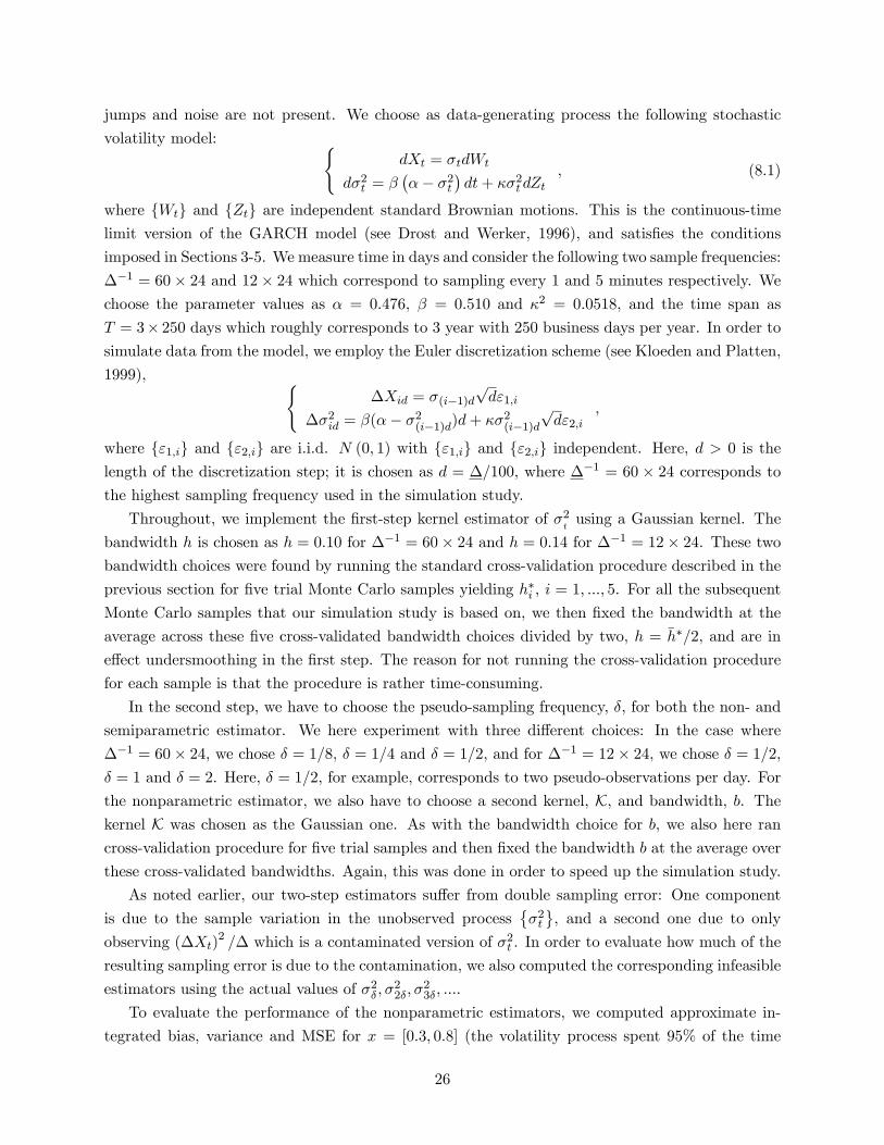
jumps and noise are not present. We choose as data-generating process the following stochastic

volatility model: dXt = σtdWt

dσ2t = β

(α− σ2

t

)dt+ κσ2

tdZt, (8.1)

where Wt and Zt are independent standard Brownian motions. This is the continuous-timelimit version of the GARCH model (see Drost and Werker, 1996), and satisfies the conditions

imposed in Sections 3-5. We measure time in days and consider the following two sample frequencies:

∆−1 = 60× 24 and 12× 24 which correspond to sampling every 1 and 5 minutes respectively. We

choose the parameter values as α = 0.476, β = 0.510 and κ2 = 0.0518, and the time span as

T = 3× 250 days which roughly corresponds to 3 year with 250 business days per year. In order to

simulate data from the model, we employ the Euler discretization scheme (see Kloeden and Platten,

1999), ∆Xid = σ(i−1)d

√dε1,i

∆σ2id = β(α− σ2

(i−1)d)d+ κσ2(i−1)d

√dε2,i

,

where ε1,i and ε2,i are i.i.d. N (0, 1) with ε1,i and ε2,i independent. Here, d > 0 is the

length of the discretization step; it is chosen as d = ∆/100, where ∆−1 = 60 × 24 corresponds to

the highest sampling frequency used in the simulation study.

Throughout, we implement the first-step kernel estimator of σ2tusing a Gaussian kernel. The

bandwidth h is chosen as h = 0.10 for ∆−1 = 60× 24 and h = 0.14 for ∆−1 = 12× 24. These two

bandwidth choices were found by running the standard cross-validation procedure described in the

previous section for five trial Monte Carlo samples yielding h∗i , i = 1, ..., 5. For all the subsequent

Monte Carlo samples that our simulation study is based on, we then fixed the bandwidth at the

average across these five cross-validated bandwidth choices divided by two, h = h∗/2, and are in

effect undersmoothing in the first step. The reason for not running the cross-validation procedure

for each sample is that the procedure is rather time-consuming.

In the second step, we have to choose the pseudo-sampling frequency, δ, for both the non- and

semiparametric estimator. We here experiment with three different choices: In the case where

∆−1 = 60× 24, we chose δ = 1/8, δ = 1/4 and δ = 1/2, and for ∆−1 = 12× 24, we chose δ = 1/2,

δ = 1 and δ = 2. Here, δ = 1/2, for example, corresponds to two pseudo-observations per day. For

the nonparametric estimator, we also have to choose a second kernel, K, and bandwidth, b. Thekernel K was chosen as the Gaussian one. As with the bandwidth choice for b, we also here rancross-validation procedure for five trial samples and then fixed the bandwidth b at the average over

these cross-validated bandwidths. Again, this was done in order to speed up the simulation study.

As noted earlier, our two-step estimators suffer from double sampling error: One component

is due to the sample variation in the unobserved processσ2t

, and a second one due to only

observing (∆Xt)2 /∆ which is a contaminated version of σ2

t . In order to evaluate how much of the

resulting sampling error is due to the contamination, we also computed the corresponding infeasible

estimators using the actual values of σ2δ , σ

22δ, σ

23δ, ....

To evaluate the performance of the nonparametric estimators, we computed approximate in-

tegrated bias, variance and MSE for x = [0.3, 0.8] (the volatility process spent 95% of the time

26

within that interval in our samples). The integrated squared bias of the drift estimates was esti-

mated by BIAS2 =∫ 0.8

0.3 [α (x)− α (x)]2 dx where α (x) = 1S

∑Ss=1 αs (x) and αs (x) was the esti-

mated drift in the s-th sample over S(= 400) Monte Carlo replications we generated. Similarly,

the integrated variance and MSE were estimated by VAR = 1S

∑Ss=1

∫ 0.80.3 [αs (x)− α (x)]2 dx and

MSE = 1S

∑Ss=1

∫ 0.80.3 [αs (x)− α (x)]2 dx = BIAS2 + VAR.

In Table 1, we report integrated squared bias, variance and MSE of the drift and diffusion

estimators for the first sampling scheme, ∆−1 = 60 × 24. In columns 1 and 2, the performance of

the infeasible and feasible nonparametric drift estimator is reported. As predicted by theory, the

performance of the infeasible estimator deteriorates as the sampling frequency δ−1 decreases. As

expected, this is not in general the case for the feasible two-step estimator however: Too small or

too large choices of δ−1 yield poor estimates; here, δ = 1/4 gives the best performance of the three

different choices. A similar pattern is found in columns 3 and 4 where the results of the diffusion

estimators are reported: The MSE of the infeasible diffusion estimator increases with δ, while the

feasible one performs best at the intermediate choice of δ = 1.

In Figures 1-4, we have plotted the pointwise means of the infeasible and feasible estimators for

δ = 1/4 together with their 95% confidence intervals. The plots mirror the results of Table 1 with

little difference between the 1-step and 2-step estimators, which is rather encouraging.

In Table 2, we report the same results but now for the second sampling scheme, ∆−1 = 12×24.

In general the performance of the feasible estimator is worse due to less precise estimates ofσ2t

in the first step. To control the added estimation error in the second step, we here have chosen

δ = 1/2, δ = 1 and δ = 2 in the second step. The same picture appears as for the higher frequency.

Again, the intermediate choice of δ = 1 yields the most precise estimates with too low or too high

choices of δ reducing precision.

Two results of the simulation study that may seem surprising are: First, the 2-step estimators

outperform the 1-step ones in some cases (∆−1 = 60× 24 and δ = 1/4; ∆−1 = 12× 24 and δ = 1).

This seems to indicate that the pre-smoothing of data actually improves on the performance of

the Nadaraya-Watson estimators in some cases. Second, the MSE of the drift estimator with

∆−1 = 12×24 and δ = 1 is lower than the one with ∆−1 = 60×24 and δ = 1/4. This is most likely

due to the fact that the bandwidths h and b in our simulation study have been chosen in a rather

ad hoc manner. It further emphasizes the importance of developing good, data-driven bandwidth

selection procedures for our estimators.

We next analyze the finite-sample performance of the parametric estimators. We maintain the

SV model in eq. (8.1) as the DGP with the same parameter values. For this model, the parametric

least-squares estimators can be written in the closed form: α = −aOLS/bOLS, β = −bOLS, andκ2 = cOLS, where, with Xτ j = (1, σ2

τ j )F,(

aOLS

bOLS

)=

1

δ

(N−1∑j=1

Xτ jX′τ j

)−1(N−1∑j=1

Xj∆σ2τ j+1

), cOLS =

1

δ

(N−1∑j=1

σ8τ j

)−1(N−1∑j=1

σ4τ j (∆σ

2τ j+1)

2

).

Tables 3 and 4 report results for the cases ∆−1 = 60× 24 and ∆−1 = 12× 24 respectively. For

both sampling frequencies, we chose, after some experimentation, three pseudo-sampling frequen-

27

cies, δ = 1/12, 1/6 and 1/4. We here note that we use smaller pseudo frequencies compared to the

nonparametric case. It appears as if parametric estimators are less affected by the first-step error,

such that we can choose a smaller δ.

In contrast to the nonparametric estimators, the infeasible estimators outperform our 2-step

estimators in all cases. Otherwise, patterns similar to those for the nonparametric estimators

appear: First, more data available in the first step (∆ = 1/ (24× 60) versus ∆ = 1/ (24× 12))

improves the quality of the spot volatility estimator which in turn leads to better performance

of the final estimators. Second, a small level of δ is not necessarily optimal; for example, with

∆ = 1/ (24× 12), the estimation results based on δ = 1/6 generally outperform the ones using

δ = 1/12. Otherwise, the performance of the parametric estimators are somewhat mixed across

the different parameters. The long-run level, α, is estimated consistently well across all sampling

schemes and is close to the infeasible estimator based on observing the volatility process. On the

other hand, relatively large biases are incurred when implementing our estimator for the mean-

reversion parameter, β: For example, in the case with ∆ = 1/ (24× 12) and δ = 1/6, the smallest

squared bias of our estimator is 14.4633×10−4 compared to 2.3990×10−4 for the infeasible estimator.

Finally, the performance of our estimator of κ2 falls somewhere in between these two cases.

Before concluding this section, we note that Zu (2014) presents some simulation results with

various parameter settings, comparing our method (for parametric models) with the one based on

the estimation of integrated volatility. His investigation suggests good performances of our method.

9 Conclusion and Extensions

We have proposed a method for the estimation of SV models in the presence of high-frequency

data. The asymptotic properties of the estimator were derived and their finite-sample precision

examined in a simulation study. Our theoretical results ignore the first-step sampling error. It

would be useful to extend our asymptotic results to include both first- and second-step sampling

errors. A first step in this direction has been made by Mammen, Rothe and Schienle (2012) in a

cross-sectional setting.

It would also be of interest to provide a complete asymptotic analysis of the jump- and noise

robust spot volatility estimator proposed in Section 3.4 and the estimators proposed Section 6

allowing for jumps in the volatility.

28

References

Aït-Sahalia, Y. and J.Y. Park (2013) Bandwidth Selection and Asymptotic Properties of Local Non-

parametric Estimators in Possibly Nonstationary Continuous-Time Models. Working paper,

Indiana University.

Altissimo, F. and A. Mele (2009) Simulated Nonparametric Estimation of Dynamic Models. Review

of Economic Studies 76, 413-450.

Andersen, T.G. and J. Lund (1997) Estimating Continuous-Time Stochastic Volatility Models of

the Short Term Interest Rate. Journal of Econometrics 77, 343-377.

Bandi, F.M. and T. Nguyen (2003) On the functional estimation of jump-diffusion models. Journal

of Econometrics 116, 293-328.

Bandi, F.M. and P.C.B. Phillips (2003) Fully Nonparametric Estimation of Scalar Diffusion Models.

Econometrica 71, 241-283.

Bandi, F.M. and P.C.B. Phillips (2007) A Simple Approach to the Parametric Estimation of Po-

tentially Nonstationary Diffusions. Journal of Econometrics, 137, 354-395.

Bandi, F.M. and R. Renò (2009) Nonparametric Stochastic Volatility. Manuscript, Graduate School

of Business, University of Chicago.

Barndorff-Nielsen, O.E. and N. Shephard (2001) Econometric Analysis of Realized Volatility and

Its Use in Estimating Stochastic Volatility Models. Journal of the Royal Statistical Society,

Series B 64, 253-280.

Barndorff-Nielsen, O.E., P.R. Hansen, A. Lunde and N. Shephard (2008) Designing realised kernels

to measure the ex-post variation of equity prices in the presence of noise, Econometrica 76,

1481-1536.

Bollerslev, T. and H. Zhou (2002) Estimating Stochastic Volatility Diffusion Using Conditional

Moments of Integrated Volatility. Journal of Econometrics 109, 33-65.

Borkovec, M. and Klüpperlberg, C. (1998) Extremal Behavior of Diffusion Models in Finance.

Extremes 1, 47-80.

Chacko, G. and L.M. Viceira (2003) Spectral GMM Estimation of Continuous-Time Processes.

Journal of Econometrics 116, 259-292.

Comte, F. ,V. Genon-Catalot and Y. Rozenholc (2009) Nonparametric Adaptive Estimation for

Integrated Diffusions. Stochastic Processes and their Applications 119, 811-834.

Comte, F. and E. Renault (1996) Long Memory Continuous Time Models, Journal of Econometrics

73, 101-149.

29

Corradi, V. and W. Distaso (2006) Semiparametric Comparison of Stochastic Volatility Models via

Realized Measures. Review of Economic Studies 73, 635-677.

Creel, M. and D. Kristensen (2014) ABC of SV: Limited Information Likelihood Inference in Sto-

chastic Volatility Jump-Diffusion Models. CREATES Research Paper 2014-30, University of

Aarhus.

Drost, F.C. and B.J.M. Werker (1996) Closing the GARCH gap: Continuous time GARCH mod-

eling. Journal of Econometrics 74, 31-57.

Dzhaparidze, K. and J.H. van Zanten (2001) On Bernstein-type Inequalities for Martingales. Sto-

chastics Processes and their Applications 93, 109-117.

Fan, J. and Y. Wang (2008) Spot Volatility Estimation for High-Frequency Data, Statistics and its

Interface 1, 279-288.

Florens-Zmirou, D. (1989) Approximate Discrete Time Schemes for Statistics of Diffusion Processes.

Statistics 20, 547-557.

Florens-Zmirou, D. (1993) On Estimating the Diffusion Coeffi cient from Discrete Observations.

Journal of Applied Probability 30, 790-804.

Gallant, A. R., D. Hsieh, and G. Tauchen (1997) Estimation of Stochastic Volatility Models with

Diagnostics. Journal of Econometrics 81, 159—192.

Gao, J., S. Kanaya, D. Li and D. Tjøstheim (2015) Uniform Consistency for Nonparametric Esti-

mators in Null Recurrent Time Series. Forthcoming in Econometric Theory.

Gijbels, I., Lambert, A., and Qiu, P. (2007) Jump-preserving Regression and Smoothing Using

Local Linear Fitting: A Compromise. Annals of the Institute of Statistical Mathematics 59,

235—272.

Hansen, B.E. (2008) Uniform Convergence Rates for Kernel Estimation with Dependent Data,

Econometric Theory 24, 726-748.

Has’minskiı, R.Z. (1980) Stochastic Stability of Differential Equations, Stijthoff & Noordoff Inter-

national Publishers B.V., Alphen aan denRijn.

Hoffman, M., A. Munk and J. Schmidt-Hieber (2012) Adaptive wavelet estimation of the diffusion

coeffi cient under additive error measurements. Annales de l’Institut Henri Poincaré- Probabil-

ités et Statistiques 48, 1186-1216.

Jacod, J. (2006) Parametric Inference for Discretely Observed Non-Ergodic Diffusions. Bernoulli

12, 383-401.

30

Jacod, J., Y. Li, P. Mykland, M. Podolskij and M. Vetter (2009) Microstructure Noise in the

Continuous Xase: The Pre-Averaging Approach, Stochastic Processes and their Applications

119, 2249-2276.

Jiang, G.J. and J.L. Knight (1997) A Nonparametric Approach to the Estimation of Diffusion

Processes, with An Application to A Short-term Interest Rate Model. Econometric Theory 13,

615-645.

Jiang, G.J. and J.L. Knigh (1999) Finite Sample Comparison of Alternative Estimators of Itô

Diffusion Processes: A Monte Carlo Study. Journal of Computational Finance 2, 5-38.

Kanaya, S. (2014) Uniform Convergence Rates of Kernel-Based Nonparametric Estimators for Con-

tinuous Time Diffusion Processes: A Damping Function Approach. Manuscript, University of

Aarhus.

Kanaya, S. and D. Kristensen (2015) Optimal Sampling and Bandwidth Selection for Nonparametric

Kernel Estimators of Diffusion Processes. Manuscript, University of Aarhus.

Karlin, S. and H.M. Taylor (1981) A Second Course in Stochastic Processes, Academic Process,

New York.

Karatzas, I. and S.E. Shreve (1991) Brownian Motion and Stochastic Calculus. Second edition,

Springer.

Kloeden, P.E. and E. Platen (1999) Numerical Solution of Stochastic Differential Equations, 2nd

ed. Springer-Verlag.

Kristensen, D. (2010a) Nonparametric Filtering of the Realized Spot Volatility: A Kernel-based

Approach. Econometric Theory 26, 60-93.

Kristensen, D. (2010b) Pseudo-Maximum Likelihood Estimation in Two Classes of Semiparametric

Diffusion Models. Journal of Econometrics 156, 239-259.

Mammen, E., C. Rothe and M. Schienle (2012) Nonparametric Regression with Nonparametrically

Generated Covariates. Annals of Statistics 40, 1132-1170.

Mammen, E., C. Rothe and M. Schienle (2013) Semiparametric Estimation with Generated Co-

variates, Manuscript, Columbia University.

Malliavin, P. and M. Mancino (2002) Fourier Series Method for Measurement of Multivariate

Volatilities, Finance & Stochastics 6, 49-61.

Malliavin, P. and M. Mancino (2009) A Fourier Transform Method for Nonparametric Estimation

of Volatility, Annals of Statistics 37, 1983-2010.

Mancini, C. (2009) Non-parametric Threshold Estimation for Models with Stochastic Diffusion

Coeffi cient and Jumps. Scandinavian Journal of Statistics 36, 270-296.

31

Mancini, C., V. Mattiussi, and R. Renò (2012) Spot Volatility Estimation Using Delta Sequences.

DiMaD Working Paper, No 2012-10, Universita’degli Studi di Firenze.

Newey, W.K., J.L. Powell and F. Vella (1999) Nonparametric Estimation of Triangular Simultane-

ous Equations Models. Econometrica 67, 565-603.

Newey, W.K. and D. McFadden (1994) Large Sample Estimation and Hypothesis Testing. Handbook

of Econometrics Vol. IV, 2111-2245 (R. Engle and D. McFadden, eds.), North Holland.

Phillips, P.C.B and Yu, J. (2005) Jackknifing Bond Option Prices. Review of Financial Studies, 18,

707-742.

Prakasa Rao, B.L.S (1988) Statistical Inference from Sampled Data for Stochastic Processes. Con-

temporary Mathematics, 80 249-284. American Mathematical Society, Providence, RI.

Podolskij, M. and M. Vetter (2009a) Estimation of Volatility Functionals in the Simultaneous

Presence of Microstructure Noise and Jumps, Bernoulli 15, 634-658.

Podolskij, M. and M. Vetter (2009b) Bipower-type Estimation in a Noisy Diffusion Setting, Sto-

chastic Processes and their Applications 119, 2803-2831.

Renò, R. (2006) Nonparametric Estimation of Stochastic Volatility Models. Economics Letters 90,

390-395.

Renò, R. (2008) Nonparametric Estimation of the Diffusion Coeffi cient of Stochastic Volatility

Models. Econometric Theory 24, 1174-1206.

Revuz, D. and M. Yor (1999) Continuous Martingales and Brownian Motion. Third edition,

Springer.

Sperlich, S. (2009) A Note on Nonparametric Estimation with Predicted Variables. Econometrics

Journal 12, 382-395.

Sørensen, M. (2009) Effi cient Estimation for Ergodic Diffusions Sampled at High Frequency. Man-

uscript, Department of Mathematical Sciences, University of Copenhagen.

Todorov, V. (2009) Estimation of Continuous-Time Stochastic Volatility Models with Jumps Using

High-Frequency Data. Journal of Econometrics 148, 131-148.

Wang, Q. and N. Chan (2014) Uniform Convergence Rates for a Class of Martingales with Appli-

cation in Non-linear Cointegrating Regression. Bernoulli 20, 1-393.

Xiao, Z. O.B. Linton, R.J. Carroll and E. Mammen (2003) More Effi cient Local Polynomial Es-

timation in Nonparametric Regression With Autocorrelated Errors. Journal of the American

Statistical Association 98, 980-992.

32

Yoshida, N. (1992) Estimation for Diffusion Processes from Discrete Observations. Journal of Mul-

tivariate Analysis 41, 220-242.

Zhang, L., P.A. Mykland and Y. Aït-Sahalia (2005) A Tale of Two Time Scales: Determining

Integrated Volatility With Noisy High-Frequency Data, Journal of the American Statistical

Association 100, 1394-1411.

Zu, Y. and H.P. Boswijk (2014) Estimating Spot Volatility with High-frequency Financial Data.

Journal of Econometrics 181, 117—135.

Zu, Y. (2014) Estimating Stochastic Volatility Models with High-Frequency Data: A Monte Carlo

Investigation, Working paper, City University London.

A Proofs of Theorems

A.1 Proofs for Section 3

We first state a result on almost sure Hölder continuity of the process t 7→ σ2t uniformly over the

infinite time interval [0,∞):

Lemma A.1 Suppose that Assumption A.3 holds. Then, for any γ ∈ (0, ρ/λ), there exists some

constant D (> 0) such that

Pr

ω ∈ Ω

∣∣∣∣∣∣∃∆ (ω) s.t. sup|t−s|∈(0,∆(ω)); s,t∈[0,∞)

∣∣σ2t (ω)− σ2

s (ω)∣∣

|t− s|γ ≤ D

= 1. (A.1)

Proof of Theorem 3.1. We expand the spot volatility estimator and analyze each of the terms

in this expansion. In what follows, we extend the processes µt andσ2t

by setting µt = σ2

t = 0

for t < 0. By Ito’s lemma for continuous semimartingales,

(∆Xti)2 = 2

∫ ti

ti−1

(∫ s

ti−1

µudu+

∫ s

ti−1

σudWu

)µsds

+2

∫ ti

ti−1

(∫ s

ti−1

µudu+

∫ s

ti−1

σudWu

)σsdWs +

∫ ti

ti−1

σ2sds.

Thus, supτ∈[√h,T−

√h]

∣∣σ2τ − σ2

τ

∣∣ ≤ 2R1 + 2R2 + 2R3 + 2R4 +R5, where

R1 : = supτ∈[0,T ]

∣∣∣∣∣∑n

i=2Kh (ti−1 − τ)

∫ ti

ti−1

(∫ s

ti−1

µudu

)µsds

∣∣∣∣∣ ;R2 : = sup

τ∈[0,T ]

∣∣∣∣∣∑n

i=2Kh (ti−1 − τ)

∫ ti

ti−1

(∫ s

ti−1

σudWu

)µsds

∣∣∣∣∣ ;

33

R3 : = supτ∈[0,T ]

∣∣∣∣∣∑n

i=2Kh (ti−1 − τ)

∫ ti

ti−1

(∫ s

ti−1

µudu

)σsdWs

∣∣∣∣∣ ;R4 : = sup

τ∈[0,T ]

∣∣∣∣∣∑n

i=2Kh (ti−1 − τ)

∫ ti

ti−1

(∫ s

ti−1

σudWu

)σsdWs

∣∣∣∣∣ ;R5 : = supτ∈[

√h,T−

√h]

∣∣∣∣∣∑n

i=2Kh (ti−1 − τ)

∫ ti

ti−1

σ2sds− σ2

τ

∣∣∣∣∣ .We show below that

R1 = OP

(∆T (2+2l1)/(2+p)h−2/(2+p)

); (A.2)

R2 = OP

(∆1/2T η0 (T/h)f0

); (A.3)

R3 = OP

(√h−1∆ log(1/∆)∆1/2T η0

[T 2/h∆ log (1/∆)

]f0) ; (A.4)

R4 = OP

(√h−1∆ log(1/∆)T 2l2/(2+q)

[T 2/h∆ log(1/∆)

]2/(2+q))

; (A.5)

R5 = OP (hγ) , (A.6)

where η0 := l1/ (2 + p) + l2/ (2 + q) and f0 := 1/ (2 + p) + 1/ (2 + q). We note that R1 is of smaller

order than R2, R3 is of smaller order than R4 by eq. (3.2), and that R2 is of the same order as R4

since

R2 = OP (R4)×T (1+l1)(2+q)−(3+l2)(2+p)hp(2+q)/2

[h∆2 log(1/∆)

](2+p)1/(2+q)(2+p)

× [log(1/∆)]−q/2(2+q) = oP (R4),

where the last equality is due to eq. (3.3). As a result, R4 and R5 are the dominant terms, yielding

the claimed result.

Proof of eq. (A.2). By Jensen’s inequality and max1≤i≤n maxs∈[ti−1,ti] |s− ti−1| ≤ ∆,∣∣∣∣∣∫ ti

ti−1

(∫ s

ti−1

µudu

)µsds

∣∣∣∣∣ ≤∫ ti

ti−1

(∫ ti

ti−1

|µu| du)|µs| ds =

(∫ ti

ti−1

|µs| ds)2

≤ ∆

∫ ti

ti−1

µ2sds.

Thus, for a given sequence φT ,

R1 ≤ ∆ supτ∈[0,T ]

∑n

i=2|Kh (ti−1 − τ)|

∫ ti

ti−1

|µs|2 1 |µs| ≤ φT ds

+ ∆ supτ∈[0,T ]

∑n

i=2|Kh (ti−1 − τ)|

∫ ti

ti−1

|µs|2 1 |µs| > φT ds =: R11 +R12. (A.7)

Here, R11 is the truncated version of R1 and satisfies

R11 = ∆ supτ∈[0,T ]

n∑i=2

1

h

∫ ti

ti−1

∣∣∣∣K (s− τh +tj−1 − s

h

)∣∣∣∣ |µs|2 1 |µs| ≤ φT ds

= ∆ supτ∈[0,T ]

∫ (T−τ)/h

−τ/h|K (u+O (∆/h))|

∣∣µuh+τ

∣∣2 1∣∣µuh+τ

∣∣ ≤ φT du≤ ∆φ2

T ×∫ ∞−∞|K (u+O (∆/h))| du = O

(∆φ2

T

). (A.8)

34

Note that∫∞−∞ |K (u+O (∆/h))| du →

∫∞−∞ |K (u)| du as ∆/h → 0 by the bounded convergence

theorem. As for R12,

E [R12] ≤ E[∆K

1

h

∫ T

0|µs|2 1 |µs| > φT ds

]≤ K

hφpT∆T sup

s≤TE[|µs|2+p

]= O

(∆T 1+l1

hφpT

), (A.9)

where the last equality follows from Assumption A.1. Now, choose φT = T (1+l1)/(p+2)h−1/(2+p).

Then, eqs. (A.7)-(A.9) establish that R1 = OP(∆T (2+2l1)/(2+p)h−2/(2+p)

).

Proof of eq. (A.3). By an application of Hölder’s inequality, we have R2 ≤√R21 ×R22, where

R21 : = supτ∈[0,T ]

∑n

i=2|Kh (ti−1 − τ)|

(∫ ti

ti−1

|µs| ds)2

;

R22 : = supτ∈[0,T ]

∑n

i=2|Kh (ti−1 − τ)|

(max

s∈[ti−1,ti]

∣∣∣∣∣∫ s

ti−1

σudWu

∣∣∣∣∣)2

.

With φT being as before: R21 = O(∆φ2

T

)+OP

(∆T (1+l1)/

(hφpT

))by the same arguments as for

R1. Let Λ2ti := maxs∈[ti−1,ti]

∣∣∣∫ sti−1σudWu

∣∣∣2 ≤ φ2T + Λ2

ti1

Λti > φT

for any positive sequence φT .

Then, analogously to the analysis of R12,

E [R22] = ∆−1φ2T supτ∈[0,T ]

∑n

i=2|Kh (ti−1 − τ)|∆ +

K

hφqT

∑n

i=2E[Λ2+qti

]= O

(∆−1φ

2T

)+O

(∆q/2T 1+l2

hφqT

),

where the last equality uses that

supτ∈[0,T ]

∑n

i=2|Kh (ti−1 − τ)|∆ ≤

∫ ∞−∞|K (u+O (∆/h))| du = O (1) ; and

maxi∈2,...,n

E[Λ2+qti

]≤ max

i∈2,...,nCE

[∣∣∣∫ titi−1σ2udu

∣∣∣(2+q)/2]≤ C∆(q/2)+1 sup

s≤TE[σ2+qs

]= O(∆(q/2)+1T l2).

The latter bound is due to the Burkholder-Davis-Gundy (BDG) and Jensen inequalities, and As-

sumption A.2. With φT = T (1+l1)/(2+p)h−1/(2+p) and φT = ∆1/2T (1+l2)/(2+q)h−1/(2+q),

R2 =

O(∆φ2

T

)+OP

(∆T (1+l1)

hφpT

)1/2OP

(∆−1φ

2T

)+OP

(∆q/2T 1+l2

hφqT

)1/2

= OP

(∆1/2T [(1+l1)/(2+p)+(1+l2)/(2+q)]h−[1/(2+p)+1/(2+q)]

)= OP

(∆1/2T η0(T/h)f0

). (A.10)

Proof of eq. (A.4). First, let Tk := τ ∈ [0, T ] : |τ − τk| ≤ T/νT , k = 1, . . . , νT , be a covering of

[0, T ], where νT is the number of intervals and τk is the center of each Tk. We also let Γ (s, ti−1) :=

(∫ sti−1

µudu)σs and ΓT (s, ti−1) = Γ (s, ti−1) 1|Γ (s, ti−1)| ≤ ϕT for a sequence of positive real

35

numbers ϕT T≥1 that are specified below. Then, R3 is bounded by

R3 ≤ maxk∈1,...,νT

supτ∈Tk

∣∣∣∣∣∑n

i=2[Kh (ti−1 − τ)−Kh (ti−1 − τk)]

∫ ti

ti−1

ΓT (s, ti−1) dWs

∣∣∣∣∣+ maxk∈1,...,νT

∣∣∣∣∣∑n

i=2Kh (ti−1 − τk)

∫ ti

ti−1

ΓT (s, ti−1) dWs

∣∣∣∣∣+ supτ∈[0,T ]

∣∣∣∣∣∑n

i=2Kh (ti−1 − τ)

∫ ti

ti−1

Γ (s, ti−1) 1 |Γ (s, ti−1)| > ϕT dWs

∣∣∣∣∣= : R31 +R32 +R33.

Using Hölder’s inequality, Lipschitz continuity of K and E[∑n

i=2(∫ titi−1

ΓT (s, ti−1) dWs)2] ≤ Tϕ2

T ,

R31 ≤ maxk∈1,...,νT

supτ∈Tk

∑n

i=2[Kh (ti−1 − τ)−Kh (ti−1 − τk)]2

1/2OP

(√TϕT

)= OP

(T 2ϕT

h2∆1/2νT

). (A.11)

Next, define % (s) := ti−1 if s ∈ [ti−1, ti), and

MkT (r) :=

∑[nr]

i=2K

(ti−1 − τk

h

)∫ ti

ti−1

ΓT (s, ti−1) dWs =

∫ rT

0K

(% (s)− τk

h

)ΓT (s, % (s)) dWs.

Note thatMkT (r)

r∈[0,1]

is a continuous martingale for each (k, T ) which vanishes at zero and

has quadratic variation⟨MkT

⟩r

=∫ rT

0 K2(%(s)−τk

h

)Γ2T (s, % (s)) ds. Thus, for any c > 0 and any

sequence VT ,

Pr(∣∣∣Mk

T (1)∣∣∣ ≥ c) ≤ Pr

(∣∣∣MkT (1)

∣∣∣ ≥ c, ⟨MkT

⟩1≤ VT

)+ Pr

(⟨MkT

⟩1> VT

), (A.12)

Applying the exponential inequality for continuous martingales (see, e.g., Dzhaparidze and van Zan-

ten, 2001 or Exercise 3.16 in Ch. IV of Revuz and Yor, 1999), Pr(∣∣Mk

T (1)∣∣ ≥ c, ⟨Mk

T

⟩1≤ VT

)≤

2 exp−c2/ (2VT )

, while

⟨MkT

⟩1≤∫ T

0K2

(s− τkh

+O (∆/h)

)ds× ϕ2

T ≤ h∫ ∞−∞

K (u+O (∆/h)) du× ϕ2T ≤ CMhϕ2

T ,

(A.13)

for some constant CM > 0. With VT = CMhϕ2T , this yields Pr

(∣∣MkT (1)

∣∣ ≥ c) ≤ 2 exp−c2/ (2VT )

.

Thus, setting c = JbT , for some constant J > 0 and some sequence bT tending to zero,

Pr (R32 ≥ JbT ) ≤∑νT

k=1Pr(∣∣∣Mk

T (1)∣∣∣ ≥ JbTh) ≤ 2νT exp

− J2b2Th

2CMϕ2T

.

With νT = T 2ϕT /h2∆1/2bT and ϕT = bT

√h/ log (1/∆), we obtainR31 = OP (bT ) and Pr (R32 ≥ JbT ) ≤

2νT∆J2/2CM . Since νT = T 3/2/h√

∆ log (1/∆) ≤ ∆−c, for some c > 0, which can be checked by the

36

rate condition in (B.1), we have Pr (|R32| > JbT )→ 0 for J large enough, implying R32 = oP (bT ).

Finally, by using the BDG, Jensen and Hölder inequalities,

E [R33] ≤ nK∆1/2

hϕr0/2T

[∆

supu≤T E[|µu|2+p]1/(2+p)

sups≤T E[|σs|2+q]1/(2+q)

](2+r0)/2

= O(

∆(1+r0)/2T 1+η0(2+r0)/2/hϕ

r0/2T

), (A.14)

where we have set r0 = (1/f0) − 2 = [1/ (2 + p) + 1/ (2 + q)]−1 − 2, and f0 and η0 were defined

previously.Therefore, for the term R33 to have same rate, bT , as R31 and R32, we require

∆(1+r0)/2T 1+η0(2+r0)/2

hϕr0/2T

= bT ⇔ bT =√h−1∆ log(1/∆)∆1/2T η0

[T 2/h∆ log (1/∆)

]1/(2+r0),

where the equivalence is due to the above choice of ϕT . This establishes the desired result.

Proof of eq. (A.5). The convergence rate of R4 can be derived analogously to that of R3. Con-

struct a covering of [0, T ], UkvTk=1, where each Uk has the radius T/vT from the center τk. Let

Π (s, ti−1) := (∫ sti−1

σudWu)σs and ΠT (s, ti−1) := Π (s, ti−1) 1 |Π (s, ti−1)| ≤ ψT for some sequenceψT T≥1. Then,

R4 ≤ maxk∈1,...,vT

supτ∈Uk

∣∣∣∣∣∑n

i=2[Kh (ti−1 − τ)−Kh (ti−1 − τk)]

∫ ti

ti−1

ΠT (s, ti−1) dWs

∣∣∣∣∣+ maxk∈1,...,vT

∣∣∣∣∣∑n

i=1Kh (ti−1 − τk)

∫ ti

ti−1

ΠT (s, ti−1) dWs

∣∣∣∣∣+ supτ∈[0,T ]

∣∣∣∣∣∑n

i=1Kh (ti−1 − τk)

∫ ti

ti−1

Π (s, ti−1) 1 |Π (s, ti−1)| > ψT dWs

∣∣∣∣∣=: R41 +R42 +R43, (A.15)

By the same arguments as for R31, R41 = OP

(T 2ψT

h2∆1/2vT

); with vT = T 2ψT /h

2∆1/2bT , R41 =

OP (bT ). Define a continuous martingaleNkT (r) :=

∫ rT0 K

(%(s)−τk

h

)ΠT (s, % (s)) dWs whose quadratic

variation process⟨NkT

⟩ris computed analogously to

⟨MkT

⟩rand satisfies

⟨NkT

⟩1≤ CNhψ2

T for some

constant CN > 0. Therefore, by the same arguments as for R32 and with ψT = bT√h/ log (1/∆),

Pr (|R42| > JbT ) ≤ 2vT exp

− J2b2Th

2CNψ2T

≤ 2vT∆J2/2CN .

Since vT = T 2/h3/2√

∆ log (1/∆) and it is bounded by∆−c for some c > 0, Pr (|R42| > JbT )→ 0 for

J large enough (as ∆→ 0) so that R42 = oP (bT ). Finally, similarly to the moment bound for R33 in

eq. (A.14), E [R43] = O(

∆ρ0/4T 1+l2/2/(hψ

ρ0/2T

)), with ρ0 := (2 + q) /2− 2. Therefore, given the

above choice of ψT , for R43 = OP (bT ), we set bT =√h−1∆ log(1/∆)

[T (2+l2)/h∆ log(1/∆)

]1/(2+ρ0).

This establishes the desired result.

37

Proof of eq. (A.6). With κ (s) := (% (s)− s) /h and % (s) = ti−1 for s ∈ [ti−1, ti),

R5 ≤ supτ∈[0,T ]

∣∣∣∣∣∫ (T−τ)/h

−τ/hK (u+ κ (uh+ τ))

[σ2uh+τ − σ2

τ

]du

∣∣∣∣∣+ supτ∈[√h,T−

√h]

∣∣∣∣∣∫ (T−τ)/h

−τ/hK (u+ κ (uh+ τ)) du−

∫ ∞−∞

K (u+ κ (uh+ τ)) du

∣∣∣∣∣ supτ∈[0,T ]

σ2τ

= : R51 +R52. (A.16)

Assumption A.2 and Lemma A.1 imply that there exists ∆ > 0 such that for any ∆ ≤ ∆ and

|t− s| ≤ ∆, |σt − σs| ≤ D |t− s|γ a.s. Therefore, R51 ≤ Dhγ∫∞−∞ |K (u+O (∆/h))| |u|γ du =

Oa.s.(hγ) since

∫∞−∞ |K (u+O (∆/h))| |u|γ du ≤

∫∞−∞K

∗ (u) |u|γ du <∞, where

K∗ (u) :=

K if |u| ≤ C + ε,

|K(C)|−Kε [u− C − ε] + K if |u| ∈ (C + ε, C + 2ε],

|K (u− 2ε)| if |u| > C + 2ε,

(A.17)

for some constant ε > 0. To bound R52, we first bound supτ∈[0,T ] σ2τ : Let Vk

wTk=1 be a finite

covering of [0, T ], where Vk has center τk and radius T/wT . Then, with wT := T log (1/h),

supτ∈[0,T ]

σ2τ = max

k∈1,...,wT supτ∈Vk

∣∣σ2τ − σ2

τk

∣∣+ maxk∈1,...,wT

σ2τk≤ Oa.s.(|T/wT |γ) +

∑wTk=1 σ

2τk

= Oa.s.

(| log (1/h) |−γ) + T [log (1/h)]×OP (T l2

)= OP

(T 1+2l2/(2+q) log (1/h)

), (A.18)

where we have used sups≤T E[σ2t ] = O

(T 2l2/(2+q)

)(see Assumption A.2). Next, observe that

supτ∈[√h,T−

√h]

∣∣∣∣∣∫ (T−τ)/h

−τ/hK (u+ k (uh+ τ)) du−

∫ ∞−∞

K (u+ k (uh+ τ)) du

∣∣∣∣∣≤

∫ ∞1/√h|K (u+ k (uh+ τ))| du+

∫ 1/√h

−∞|K (u+ k (uh+ τ))| du. (A.19)

The two terms on the RHS are both O(h(m+c)/2

)for some c > 0. To see this, note that there

exists some c > 0 such that |K (x)| ≤ |x|−m−1−c for |x| large enough since∫∞−∞ x

mK (x) dx <

∞.and that κ (r) = O (∆/h) = o (1). Thus,∫∞

1/√h |K (u+ κ (uh+ τ))| du = O(|1/

√h|−m−c) =

O(h(m+c)/2

). The term

∫ 1/√h

−∞ |K (u+ k (uh+ τ))| du can be treated in the same way. In total,R52 = OP

(h(m+c)/2T 1+2l2/(2+q) log (1/h)

)= oP (hγ), where we have used log (1/h)hc/2 = o (1) and

hm−2γT 2+4l2/(2+q) = O(1) as imposed in Assumption B.1. This yields the desired result.

For the proof of Theorem 3.2, we first derive the uniform convergence rate of |Xt −Xt|:

Lemma A.2 Suppose that Assumptions A.1-A.3 and B.1-B.2 and K.1-K.2 are satisfied. Then, as∆,∆s → 0, and T/∆, T/∆s →∞, Xt defined in eq. (3.7) satisfies

supτ∈[√h,T−

√h] |Xt −Xt| = OP

(√a(T 1+l2/a)1/(2+q) +

√a−1∆s log(1/∆s)

), (A.20)

38

Proof of Theorem 3.2. Observe that

σ2NR,τ =

∑n

i=1Kh (ti−1 − τ)

[(Xti −Xti−1) + (Xti − Xti−1)− (Xti −Xti−1)

]2

= σ2τ +

∑n

i=1Kh (ti−1 − τ)

[(Xti − Xti−1)− (Xti −Xti−1)

]2

−2∑n

i=1Kh (ti−1 − τ)

(Xti −Xti−1

) [(Xti − Xti−1)− (Xti −Xti−1)

]= : σ2

τ + U1 (τ)− 2U2 (τ) ,

where

supτ∈[√a,T−

√a] |U1 (τ)| ≤ supτ∈[0,T ]

∑ni=1 |Kh (ti−1 − τ)|∆︸ ︷︷ ︸

=O(1)

× (4/∆) supt∈[√a,T−

√a] |Xt −Xt|2;

supτ∈[√a,T−

√a] |U2 (τ)| ≤ supτ∈[0,T ]

∑ni=1 |Kh (ti−1 − τ)|

[∫ titi−1|µs|ds+ |

∫ titi−1

σsdWs|]

×2 supt∈[√a,T−

√a] |Xt −Xt|.

By the same arguments as those for R1 and R2 in the proof of Theorem 3.1, and by eq. (3.12),

supτ∈[0,T ]

∑ni=1 |Kh (ti−1 − τ)|

[∫ titi−1|µs|ds+ |

∫ titi−1

σsdWs|]

= OP (∆−1/2(T (1+l2)/a)1/(2+q)).

Given this expression and Lemma A.2, supτ∈[√a,T−

√a] |U1 (τ)| = oP

(supτ∈[

√a,T−

√a] |U2 (τ)|

)and

so (3.13) holds. Finally, to derive the rate of supτ∈[√h,T−

√h]

∣∣σ2τ − σ2

τ

∣∣, note that ∆−1a → 0 and

h−1∆→ 0 since ϑNRT,∆,∆s

→ 0. These in turn imply that a/h→ 0 and [√h, T −

√h] ⊂ [

√a, T −

√a].

Therefore, the result of Theorem 3.1 and the triangular inequality imply the desired result.

Proof of Theorem 3.3. We write the continuous component of Xt as X∗t =∫ t

0 µsds+∫ t

0 σsdWs.

Thus, we have Xt = X∗t +∑Nt

j=1 κj . By Lemma 3.1, we have for ∆ small enough,

σ2JR,τ − σ2

τ =∑n

i=1Kh (ti−1 − τ) [X∗ti −X

∗ti−1 ]

21Nti −Nti−1 = 0

− σ2

τ

=σ2τ − σ2

τ

−∑n

i=1Kh (ti−1 − τ) [X∗ti −X

∗ti−1 ]

21Nti −Nti−1 6= 0

,

where σ2τ is the no-jump and no-noise estimator based on observingX

∗t , and so supτ∈[

√h,T−

√h]

∣∣σ2τ − σ2

τ

∣∣ =

OP (ϑ∆,T ). The second term is bounded by

NT maxi∈2,...,n

Kh (ti−1 − τ)[∫ titi−1

µsds+∫ titi−1

σsdWs

]2

≤ 2NT K

h

[∆ maxi∈2,...,n

∫ titi−1|µs|2 ds+ max

i∈2,...,n|∫ titi−1

σsdWs|2], (A.21)

where we have used (A+B)2 ≤ 2(A2 +B2

)and Jensen’s inequality. We note that E [NT ] ≤ λT

and can show maxi∈2,...,n∫ titi−1|µs|2 ds = OP (∆p/(2+p)T 2(1+l1)/(2+p)) in the same way as eq. (B.6)

was derived. To find a bound of maxi∈2,...,n |∫ titi−1

σsdWs|, we use the exponential inequality for

39

continuous martingales (Exercise 3.16 in Ch. IV of Revuz and Yor, 1999),

Pr(

maxi∈2,...,n |∫ titi−1

σsdWs| ≥ J)

≤n∑i=2

Pr(|∫ titi−1

σsdWs| ≥ J,∫ titi−1

σ2sds ≤ ηT

)+ Pr

(∫ titi−1

σ2sds > ηT

)≤ 2n exp

−J2/2ηT

+ n∆(2+q)/2 sup

s≤TE[|σs|2+q

]η−q/2T︸ ︷︷ ︸

O(∆q/2T 1+l1η−q/2T )

.

By letting ηT = J2∆T 2(1+l1)/q and J = J (1+q)√

[∆ log (1/∆)]T 2(l2+1)/q for any J > 0, we have

Pr

(maxi∈2,...,n |

∫ titi−1

σsdWs| ≥ J (1+q)√

[∆ log (1/∆)]T 2(1+l2)/q

)≤ 2n∆(1/2)J2q +O

(J−q

).

Having J large enough, the majorant side can be made arbitrarily small as ∆→ 0 and T/∆→∞(by the rate condition in (B.1)), and thus

maxi∈2,...,n |∫ titi−1

σsdWs| = OP (√

[∆ log (1/∆)]T 2(1+l2)/q).

A.2 Proofs for Section 4

The following lemmas will be used in the proofs:

Lemma A.3 Assume σ2τ satisfies eq. (4.1) and Assumptions A.2’and K.3 are satisfied. If there

exists some q > 0 such that (ϑN/b)q = O (b), then, as T →∞, δ → 0 and b→ 0,

α (x)− α (x) = OP

(ϑN/bδ

1/2)

+OP (ϑN/δ) . (A.22)

Lemma A.4 Assume that Assumptions A.2’ and K.3 hold. If δγ/b → 0 and Tb → ∞, thenα (x)

P→ α (x). If in addition Tbδ2γ → 0 and Tb5 = O (1), then

√Tb[α (x)− α (x)− b2 × biasα (x)]

d→ N

(0, β4 (x)

∫ ∞−∞K2 (z) dz

),

where biasα (x) is given in Theorem 4.1.

Lemma A.5 Assume σ2τ satisfies eq. (4.1) and Assumptions A.2’and K.3 are satisfied. If there

exists some q (> 0) such that (ϑN/b)q = O (b), then, as N →∞ and b, δ → 0 with ϑN/δ1−γ → 0,

β2

(x)− β2(x) = OP (ϑN/b) +OP

(ϑN/δ

1−γ) .Lemma A.6 Assume that Assumptions A.2’and K.3 hold. If N →∞, b→ 0 with δγ/b→ 0 and

Nb→∞, then β2(x)

P→ β2 (x). If in addition Nbδ2γ → 0 and Nb5 = (1), then

√Nb[β

2(x)− β2 (x)− b2 × biasβ2 (x)]

d→ N

(0, 4β2 (x)

∫ ∞−∞K2 (z) dz

),

where biasβ2 (x) is given in Theorem 4.2.

40

Proof of Theorem 4.1. As in eq. (4.2), we split up α (x) − α (x) into two terms. The first

term of the RHS of eq. (4.2) converges to zero by Lemma A.3 under Assumption B-NDR(i). Note

that since γ ∈ (0, 1/2) and δγ/b → 0, we have δ1/2 < δγ < b (for δ and h small enough), and

ϑN/δ > ϑN/δγδ1/2 > ϑN/bδ

1/2. Therefore, ϑN/δ → 0 and δγ/b → 0 lead to ϑN/bδ1/2 → 0.

Noting also that ϑN/bδ1/2 → 0 and δγ/b→ 0 respectively imply ϑN/b < δ1/2 and δ1/2 < b1/2γ , the

condition of Lemma A.3 below is satisfied with q = 1/2γ. The convergence of the second term is

investigated in Lemma A.4 below. Assumption B-NDR(ii) ensures that the first term α (x)− α (x)

has no effect such that the asymptotic distribution is completely determined by α (x)− α (x).

Proof of Theorem 4.2. We follow the same strategy as in the proof of Theorem 4.1: First, write

β2

(x)−β2 (x) = [β2

(x)−β2(x)]+[β

2(x)−β2 (x)], where the two terms on the RHS are analyzed in

Lemmas A.5 and A.6 (see below), respectively. Note that ϑN/δ1−γ → 0 and δγ/b→ 0 respectively

imply ϑN < δ1−γ and δ1−γ < b1−γγ , and thus ϑN/b < b

1−γγ−1

= b1−2γγ → 0 since γ ∈ (0, 1/2).

Therefore, the condition of Lemma A.5 is satisfied with q = (1− 2γ) /γ. Assumption B-NDI(ii)

ensures that β2

(x)− β2(x) = oP (1/

√Nb), and thus the asymptotic distribution is determined by√

Nb[β

2(x)− β2 (x)

].

A.3 Proofs for Sections 5-7

To derive the asymptotic results for the proposed estimators, we re-define the objective functions.

Instead of Qk (θk) (for k = 1, 2) in eq. (2.5), we consider the following objective functions:

R1

(θ1, σ

2)

: =1

T

∑N−1

j=1α(σ2

τ j+1 ; θ1)[α(σ2

τ j+1 ; θ1)δ − 2(σ2τ j+1 − σ

2τ j )],

R2

(θ2, σ

2)

: =1

T

∑N−1

j=1β2(σ2

τ j+1 ; θ2)[β2(σ2

τ j+1 ; θ2)δ − 2(σ2τ j+1 − σ

2τ j )

2].

The maximizer of Rk(θk, σ

2)is equal to the original estimator θk defined in eq. (2.4) as the

maximizer of Qk (θk). Moreover, in contrast to Qk (θk), Rk(θ1, σ

2)has a well-defined asymp-

totic limit, k = 1, 2, given by R1 (θ1) :=∫I α (y; θ1) [α (y; θ1)− 2α (y)]π (y) dy and R2 (θ2) :=∫

I β2 (y; θ2)

[β2 (y; θ2)− 2β2 (y)

]π (y) dy. The first and second order derivatives of Rk

(θ1, σ

2),

k = 1, 2, are

S1

(θ1, σ

2)

: =2

T

∑N−1

j=1∂θ1α(σ2

τ j ; θ1)[α(σ2

τ j ; θ1)δ − (σ2τ j+1 − σ

2τ j )],

H1

(θ1, σ

2)

: =2

T

∑N−1

j=1

∂θ1α(σ2

τ j ; θ1)∂θ1α(σ2τ j ; θ1)Fδ

+∂θ1θ

F1α(σ2

τ j ; θ1)[α(σ2

τ j ; θ∗1)δ − (σ2

τ j+1 − σ2τ j )]

;

H1 (θ1) : = 2E[∂θ1α

(σ2t ; θ1

)∂θ1α

(σ2t ; θ1

)F];

41

and

S2

(θ2, σ

2)

: =2

T

∑N−1

j=1∂θ2β

2(σ2τ j ; θ2)

[β2(σ2

τ j ; θ2)δ − (σ2τ j+1 − σ

2τ j )

2]

;

H2

(θ2, σ

2)

: =2

T

∑N−1

j=1

∂θ2β

2(σ2τ j ; θ2)∂θ2β

2(σ2τ j ; θ2)Fδ

+∂θ2θ

F2β2(σ2

τ j ; θ2)[β2(σ2

τ j ; θ∗2)δ − (σ2

τ j+1 − σ2τ j )

2]

;

H2 (θ2) : = 2E[∂θ2β

2(σ2t ; θ2

)∂θ2β

2(σ2t ; θ2

)F].

We first state the asymptotic distribution of the infeasible estimators:

Lemma A.7 Suppose that Assumption A.2’is satisfied.

(i) If A-SDR holds, then

supθk∈Θk

∣∣∣Rk(θk, σ2)−Rk(θk)∣∣∣ = oP (1) ; and sup

θk∈Θk

∥∥∥Hk(θk, σ2)−Hk (θk)

∥∥∥ = oP (1) , (A.23)

with k = 1 and thus θ1P→ θ∗1. Moreover, if Tδ

2 → 0, then√T S1

(θ∗1, σ

2) d→ N(0,Ω∗1); and

√T [θ1 − θ∗1]

d→ N(0, H∗−11 Ω∗1H

∗−11 ),

where Ω∗1 and H∗1 are given in Theorem 5.1.

(ii) If A-SDI holds, then the results (A.23) hold with k = 2 and thus θ2P→ θ∗2. Moreover, if

Tδ → 0, then√NS2

(θ∗2, σ

2) d→ N(0,Ω∗2); and

√N [θ2 − θ∗2]

d→ N(0, H∗−12 Ω∗2H

∗−12 ),

where Ω∗2 and H∗2 are given in Theorem 5.2.

Next, we derive the stochastic difference between the feasible and infeasible objective function

and its derivatives:

Lemma A.8 Let σ2τ be an estimator of σ

2τ satisfying eq. (4.1). Suppose that Assumptions A.1,

A.2’, B.1’and A-SDR(iii) are satisfied. Then,

supθ1∈Θ1

∣∣∣R1

(θ1, σ

2)− R1

(θ1, σ

2)∣∣∣ = OP (ϑN/δ), (A.24)

√T∥∥∥S1

(θ∗1, σ

2)− S1

(θ∗1, σ

2)∥∥∥ = OP (T 1/2ϑN/δ), (A.25)

supθ1∈Θ1

∥∥∥H1

(θ1, σ

2)− H1

(θ1, σ

2)∥∥∥ = OP (ϑN/δ). (A.26)

Lemma A.9 Let σ2τ be an estimator of σ

2τ satisfying eq. (4.1). Suppose that Assumptions A.1,

A.2’, B.1’and A-SDI(iii) are satisfied. Then,

supθ2∈Θ2

∣∣∣R2

(θ2, σ

2)− R2

(θ2, σ

2)∣∣∣ = OP (ϑN/δ

1−γ), (A.27)

√N∥∥∥S2

(θ∗2, σ

2)− S2

(θ∗2, σ

2)∥∥∥ = OP (

√NϑN/δ

1−γ), (A.28)

supθ2∈Θ2

∥∥∥H2

(θ2, σ

2)− H2

(θ2, σ

2)∥∥∥ = OP (ϑN/δ

1−γ). (A.29)

42

We are now ready to prove Theorems 5.1-5.2:

Proof of Theorem 5.1. To prove consistency, we verify the conditions in Newey and McFad-

den (1994, Theorem 2.1): (i) compactness of the parameter space; (ii) continuity of the objective

function and its limit function; (iii) uniform convergence of the objective function; and (iv) identi-

fiability. Conditions (A-SDR.i) and (A-SDR.ii) imply (i), (ii) and (iv), and we only need to show

uniform convergence. Write

R1

(θ1, σ

2)−R1 (θ1) = [R1

(θ1, σ

2)− R1

(θ1, σ

2)] + [R1

(θ1, σ

2)−R1 (θ1)], (A.30)

where the two terms on the RHS converge uniformly by Lemma A.8 and A.7 respectively. By a Tay-

lor expansion,√T [θ1−θ∗1] = H−1

1

(θ1, σ

2)√

T S1

(θ∗1, σ

2), where θ1 is on the line segment connecting

θ1 to θ∗1. By (A.25) in Lemma A.9 and Assumption B-SDR,√T [S1

(θ∗1, σ

2)− S1

(θ∗1, σ

2)] = oP (1)

while the Hessian satisfies H1

(θ1, σ

2)− H1 (θ1) = [H1

(θ1, σ

2)− H1

(θ1, σ

2)] + [H1

(θ1, σ

2)−

H1 (θ1)]P→ 0 uniformly θ1 by Lemmas A.8 and A.7. Thus, θ1 has the same asymptotic distri-

bution as the infeasible estimator θ1, which is given in Lemma A.7.

Proof of Theorem 5.2. This follows along the same lines as the proof of Theorem 5.1, and so

is omitted.

Proof of Theorem 7.1. The details of the proof are provided at Cambridge Journals Online in

supplementary material to this article. Readers may refer to the supplementary material associated

with this article, available online.

B Proofs of Lemmas

Proof of Lemma A.1. From Assumption A.3 and Lemma D.1 (the details of Lemma D.1 are

provided online at Cambridge Journals Online in supplementary material to this article), there

exists a continuous modification σ2t of

σ2t

which is a.s. Hölder globally over [0,∞). Identifying

σ2t

with σ2

t , we have eq. (A.1).

Proof of Lemma A.2. Use that Xt =∫ t

0 µudu+∫ t

0 σudWu to write supt∈[√a,T−

√a] |Xt −Xt| ≤

S1 + S2 + S3 + S4 + S5 + S6, where

S1 : = supt∈[√a,T−

√a]

∣∣∣∣∫ T

0La (s− t)

(∫ s

0µudu

)ds−

∫ t

0µudu

∣∣∣∣ ;S2 : = sup

t∈[√a,T−

√a]

∣∣∣∣∫ T

0La (s− t)

(∫ s

0σudWu

)ds−

∫ t

0σudWu

∣∣∣∣ ;S3 : = sup

t∈[0,T ]

∣∣∣∣∣∑M

i=1La (si − t)

∫ i∆s

(i−i)∆s

(∫ s

(i−i)∆s

µudu

)ds

∣∣∣∣∣ ;

43

S4 : = supt∈[0,T ]

∣∣∣∣∣∑M

i=1La (si − t)

∫ i∆s

(i−i)∆s

(∫ s

(i−i)∆s

σudWu

)ds

∣∣∣∣∣ ;S5 : = sup

t∈[0,T ]

∣∣∣∣∣∑M

i=1

∫ i∆s

(i−i)∆s

[La (si − t)− La (s− t)]Xsds

∣∣∣∣∣ ;S6 : = sup

t∈[0,T ]

∣∣∣∣(T/M)∑M

i=1La (si − t) εi

∣∣∣∣ .By following the same steps as those for eqs. (A.2) and (A.3), S3 = OP (∆sT

(1+l1)/(2+p)a−1/(2+p))

and S4 = OP (∆1/2s T (1+l2)/(2+q)a−1/(2+q)), while we show below that:

S1 = OP (a(1+p)/(2+p)T (1+l1)/(2+p)); (B.1)

S2 = OP (√a(T 1+l2/a)1/(2+q)); (B.2)

S5 = OP (∆sa−1[T 1+l1/(2+p) + T 1/2+l2/(2+q)

]); (B.3)

S6 = OP (√a−1∆s log(1/∆s)). (B.4)

The first rate condition in eq. (3.10) of B.2(ii) yields S5 = OP (S6). It also implies that T 1+l1/(2+p) =

O(1/√

∆s/a (log T )), and so S3 = OP (S4) × T−(1+p)/(2+p)a1/(2+q)

T (1+l2)/(2+q)a1/(2+p)

√a (log T ) = oP (S4). Given the

rates of S4 and S6, S4 = OP (S6) × aqT 2(1+l2)/[log (1/∆s)]2+q1/2(2+q). This expression, together

with eq. (3.12) of B.2(ii), implies that S4 = OP (S6). Thus, S6 is dominant among the four

terms S3, S4, S5 and S6. Finally, by eq. (3.11) of B.2(ii), S1 = OP (S2) × (apT 2(1+l1))1/2(2+p) ×(a/T 1+l2)1/(2+q) = oP (S2). This yields the desired result of eq. (A.20).

Proof of eq. (B.1). Since L has compact support,∫ (T−t)/a−t/a L (v) dv − 1 = 0 for a small enough.

Thus,

S1 = supt∈[√a,T−

√a]

∣∣∣∣∣∫ (T−t)/a

−t/aL (v)

(∫ t+va

tµudu

)dv +

(∫ (T−t)/a

−t/aL (v) dv − 1

)∫ t

0µududv

∣∣∣∣∣≤

∫ ∞−∞|L (v)| dv sup

t∈[0,T ]

∫ t+c0a

t−c0a|µu| du. (B.5)

With φT = (T 1+l1/a)1/(2+p),

supt∈[0,T ]

∫ t+c0a

t−c0a|µu| du ≤ sup

t∈[0,T ]

∫ t+c0a

t−c0a|µu| 1 |µu| ≤ φT du+

∫ T

0|µu| 1 |µu| > φT du

≤ 2c0aφT +OP (T × T l1/φ1+pT ) = OP (a(1+p)/(2+p)T (1+l1)/(2+p)). (B.6)

Proof of eq. (B.2). Let Γs := sup|r|≤c0a

∣∣∣∫ s+rs σudWu

∣∣∣, where the integral ∫ st σudWu should be

44

interpreted as −∫ ts σudWu if s > t. Then,

E [S2] ≤ E

[supt∈[0,T ]

∣∣∣∣∫ T

0La (s− t) Γsds

∣∣∣∣]≤ ϕT supt∈[0,T ]

∫ T

0|La (s− t)| ds+ E

[supt∈[0,T ]

∣∣∣∣∫ T

0La (s− t) Γs1 Γs > ϕT ds

∣∣∣∣]≤ ϕT

∫ ∞−∞|L (v)| dv + (KT/a) sups∈[0,T ]E[Γ2+q

s ]/ϕq+1T = O(ϕT + aq/2T 1+l2/ϕq+1

T ),

where the first equality holds for a small enough, c.f. the analysis of eq. (B.5), the second inequality

holds since Γs (a) ≤ ϕT + Γs1 Γs (a) > ϕT , and the last equality uses the BDG and Jensen

inequalities. With ϕT =√a(T 1+l2/a2)1/(2+q), S2 = OP (

√a(T 1+l2/a)1/(2+q)).

Proof of eq. (B.3). By the differentiability of L, Assumptions A.1-A.2 and the BDG inequality,

S5 ≤ ∆sa−2 sup

t∈[0,T ]

∫ T

0L′(s− ta

+O (∆s/a)

)ds

[∫ T

0|µu| du+ sup

s≤T

∣∣∣∣∫ s

0σudWu

∣∣∣∣]

≤ ∆sa−1

∫ ∞−∞

L′ (u+O (∆s/a)) du×OP(T 1+l1/(2+p) + T 1/2+l2/(2+q)

)= OP (∆sa

−1[T 1+l1/(2+p) + T 1/2+l2/(2+q)

]). (B.7)

Proof of eq. (B.4). For grid points on the interval [0, T ]: u0 < u1 < · · · < uJT (with u0 = 0,

uJT = T , uj+1 − uj = T/JT , and (T/JT )→ 0), and for η > 0, define

Zi,T (uj) : = La (si − uj) εi1 |εi| ≤ ηT − E [La (si − uj) εi1 |εi| ≤ ηT ] ;

Zi,T (uj) : = La (si − uj) εi1 |εi| > ηT − E [La (si − uj) εi1 |εi| > ηT ] ; and

ηT : = η[M2/√a∆s log (1/∆s)]

1/(ds+1). (B.8)

Since E [εi] = 0,

S6 ≤ max1≤j≤JT

supt∈[uj−1,uj ]

(T/M)∑M

i=1|La (si − uj)− La (si − t)| |εi|

+ (T/M) max0≤j≤JT

∣∣∣∣∑M

i=1Zi,T (uj)

∣∣∣∣+ max0≤j≤JT

(T/M)∑M

i=1

∣∣∣Zi,T (uj)∣∣∣ =: S61 + S62 + S63. (B.9)

Here, |La (si − uj) − La (si − t) | ≤(T/JTa

2)L′(sj/a + O(T/JTa)) and max1≤i≤M |εi| = OP (M),

and thus

S61 ≤ (1/JTa)

∫ ∞−∞

L′(v +O(T/Ma+ T/JTa))dv ×max1≤i≤M |εi|

= OP (M/JTa) = OP (√a−1∆s log(1/∆s)), (B.10)

45

where we have set JT = M/√a∆s log(1/∆s). We wish to apply Bernstein’s inequality on S62 (see

p. 102 of Van der Vaart and Wellner, 1996) and to this end, compute the variance bound

Var[∑M

i=1 Zi,T (uj)]≤ (2/∆s)

∑M

i=1L2a (si − uj) ∆sE

[ε2i

]≤

(2/∆sa

2) ∫ T

0L2 ((s− uj) /a+O (∆s/a)) ds supi≥1E

[ε2i

]≤ O (1/∆sa)

∫ ∞−∞

L2 (v +O (∆s/a)) du ≤ C/∆sa,

for some constant C > 0. Given this and the fact that∣∣Zi,T (uj)

∣∣ ≤ 2KηT /a, Bernstein’s inequality

implies that

Pr(S62 ≥ η

√a−1∆s log(1/∆s)

)≤∑JT

j=1Pr[∣∣∣∑M

i=1 Zi,T (uj)∣∣∣ ≥ (M/T ) η

√a−1∆s log(1/∆s)

]≤

∑JT

j=12 exp

− η2 (M/T )2 [a−1∆s log(1/∆s)]/2∑M

i=1 Var[Zi,T (uj)

]+ (1/3)

(2KηT /a

)c (M/T )

√a−1∆s log(1/∆s)

≤ 2JT exp

− η2[log(1/∆s)]/2

C +(2Kc/3

)× ηT

√∆s log(1/∆s)/a

→ 0. (B.11)

The convergence in the last line occurs for η large enough (as T →∞), since JT = T/√a∆3

s log(1/∆s)

grows at most at polynomial order of 1/∆s (note that a−1 ≤ ∆−1/2T c1 and T ≤ ∆−c2 for some

c1, c2 > 0, both of which follow from eq. (3.10)), and since ηT√a∆s log(1/∆s) = η × O(1) by eq.

(3.9). Next, consider S63: First,

E[(T/M)

∑Mi=1 |La (si − uj) εi1 |εi| > ηT |

]≤ (T/M)

∑M

i=1|La (si − uj)| sup

i≥1E[|εi|ds+1]/ηdsT

≤∫ (T−uj)/a

−uj/a|L (v +O (1/aM + T/aM))| dv ×O(η−dsT ) = O(η−dsT ) uniformly over j,

where η−dsT = η−ds × o(√a−1∆s log(1/∆s)) since η

−dsT /

√a−1∆s log(1/∆s) = o (1) by eq. (B.8).

Therefore, for any η and for any T large enough,

Pr(S63 >

√a−1∆s log(1/∆s)

)≤∑JT

j=1Pr[(T/M)

∑Mi=1 |La (si − uj) εi1 |εi| > ηT | > (1/2)

√a−1∆s log(1/∆s)

]≤∑JT

j=1

∑M

i=1Pr[|La (si − uj)| |εi1 |εi| > ηT | > (1/2T )

√a−1∆s log(1/∆s)

]≤∑JT

j=1

∑M

i=1Pr [|εi| > ηT ] ≤ JTM supi≥1E[|εi|1+ds ]/η1+ds

T = O(JTM/η1+dsT ) = O(1/η1+ds),

(B.12)

which can be made arbitrarily close to zero by choosing η large enough. This completes the proof.

Proof of Lemma 3.1. The proof proceeds along the same lines as that of Theorem 1 of Mancini

(2009). The only difference between ours and her setup is that we allow for T →∞, and so we only

46

point out the modifications. Her original proof relies on three preliminary results/assumptions:

(i) the modulus of continuity of the Brownian motion Wt over [0, T ] with T < ∞ fixed; (ii)

the Brownian time-change technique of continuous martingales, i.e., the Dambis-Dubins-Schwarz

theorem; and (iii) a certain uniform boundedness condition, which is stated as eq. (14) in Mancini

(2009), which is implied by her conditions (1)-(3) of Theorem 1. We extend (i)-(iii) to allow for

T → ∞. Re. (i): The Brownian modulus-of-continuity result can be extended in the followingmanner:

Pr[lim sup∆0 supt,s∈[0,∞); |t−s|≤∆ |Wt −Ws| /

√2∆ log (1/∆) = 1

]= 1,

as shown in Kanaya (2014). Re. (ii): The Brownian time-change arguments hold irrespectively of

whether T is fixed or diverges (see Theorems 1.6, 1.9 and 1.10 in Ch. V of Revuz and Yor, 1999).

Re. (iii): The sequence ξT in A4(ii)-(iii) controls the behavior of µt andσ2t

as T → ∞,

and allows us to obtain a uniform boundedness condition analogous to her ineq. (14). The rest of

Mancini’s proof remains unchanged.

Proof of Lemma A.3. Write α (x)− α (x) = A1 +A2 +A3, where

A1 :=(1/T )

∑N−1j=1 Kb(σ2

τ j − x)(σ2τ j+1 − σ

2τ j )

(δ/T )∑N

j=1Kb(σ2τ j − x)

−(1/T )

∑N−1j=1 Kb(σ2

τ j − x)(σ2τ j+1 − σ

2τ j )

(δ/T )∑N

j=1Kb(σ2τ j − x)

;

A2 :=(1/T )

∑N−1j=1

[Kb(σ2

τ j − x)−Kb(σ2τ j − x)

](σ2τ j+1 − σ

2τ j )

(δ/T )∑N

j=1Kb(σ2τ j − x)

;

A3 :=(1/T )

∑N−1j=1 Kb(σ2

τ j−1 − x)[(σ2τ j+1 − σ

2τ j )− (σ2

τ j+1 − σ2τ j )]

(δ/T )∑N

j=1Kb(σ2τ j − x)

.

We show below that A1 = OP (ϑN/b), A2 = OP

(ϑN/bδ

1/2)and A3 = OP (ϑN/δ), which establish

the result stated in eq. (A.22). The proofs of these bounds will use the following result repeatedly:

δ

T

∑N

j=1

[Kb(σ2

τ j − x)−Kb(σ2τ j − x)

]= OP

(ϑNb

). (B.13)

Proof of eq. (B.13). Observe that

the LHS of eq. (B.13)

=1

N

∑N

j=1

1

bK′(

(σ2τ j − x)b−1 − wj(σ2

τ j − σ2τ j )b

−1)× wj(σ2

τ j − σ2τ j )b

−1

≤ sup1≤j≤N

wj

∣∣∣σ2τ j − σ

2τ j

∣∣∣ b−1

×

1

N

N∑j=1

1

b

∣∣∣K′ ((σ2τ j − x)b−1 − wj(σ2

τ j − σ2τ j )b

−1)∣∣∣1wj |σ2

τ j − σ2τ j |b−1 ≤ ε

+1

N

N∑j=1

1

b

∣∣∣K′ ((σ2τ j − x)b−1 − wj(σ2

τ j − σ2τ j )b

−1)∣∣∣1wj |σ2

τ j − σ2τ j |b−1 > ε

47

≤ OP (ϑN/b)

×

1

N

N∑j=1

1

bK∗(

(σ2τ j − x)b−1

)+

1

N

N∑j=1

K

b×(

sup1≤j≤N wj |σ2τ j − σ

2τ j |b−1

ε

)q(B.14)

= OP (ϑN/b)×OP (1) +

K

b×OP

(b

εq

), (B.15)

where the first equality holds by the mean-value theorem for some random variables 0 ≤ wj ≤ 1,

j = 1, . . . , N . The inequality (B.14) holds by eq. (4.1) and∣∣∣K′ ((σ2τ j − x)b−1 + wj(σ

2τ j − σ

2τ j )b

−1)∣∣∣1wj |σ2

τ j − σ2τ j |b−1 ≤ ε ≤ K∗

((σ2τ j − x)b−1

)(B.16)

where K∗ is some function and ε > 0, such that sup|ε|≤ε |K′((σ2τ j − x)b−1 + ε)| ≤ K∗((σ2

τ j − x)b−1).

By the last condition in K.3, such K∗ and ε exist by the same arguments used in the proof ofTheorem 3.1 with K∗ (u) being constructed in the same way as K∗ (u) in eq. (A.17). The equality

in eq. (B.15) holds since N−1∑N

j=1K∗b(σ2τ j − x) = OP (1) and wj(σ2

τ j − σ2τ j )b

−1 = OP (ϑN/b)

(uniformly over j), where the former follows from the positive recurrence of the processσ2t

and

standard arguments for kernel estimators given the properties of K∗.

Convergence of A1. The term A1 can be re-written as

A1 =(1/T )

∑N−1j=1 Kb(σ2

τ j − x)(σ2τ j+1 − σ

2τ j )

(δ/T )∑N

j=1Kb(σ2τ j − x)× (δ/T )

∑Nj=1Kb(σ2

τ j − x)× 1

N

∑N

j=1

[Kb(σ2

τ j − x)−Kb(σ2τ j − x)

].

By eq. (B.13), and the two following equations, we have A1 = OP (ϑN/b):

1

T

∑N−1

j=1Kb(σ2

τ j − x)(σ2τ j+1 − σ

2τ j ) = α (x)π (x) + oP (1) ; (B.17)

δ

T

∑N

j=1Kb(σ2

τ j − x) = π (x) + oP (1) . (B.18)

Convergence of A2. Write1

T

∑N−1j=1

[Kb(σ2

τ j − x)−Kb(σ2τ j − x)

](σ2τ j+1−σ

2τ j ) = Anu21 +Anu22 where

Anu21 :=1

T

∑N−1

j=1

[Kb(σ2

τ j − x)−Kb(σ2τ j − x)

] ∫ τ j+1

τ j

α(σ2s

)ds,

Anu22 :=1

T

∑N−1

j=1

[Kb(σ2

τ j − x)−Kb(σ2τ j − x)

] ∫ τ j+1

τ j

β(σ2s

)dZs.

Similarly to eq. (B.15) and the proof of eq. (B.13),

Anu21 = OP (ϑN/b)×OP (1) +

K

b×Op (1)×OP

(b

εq

)= OP (ϑN/b) , (B.19)

Anu22 = OP (ϑN/b)×OP

(δ−1/2

)+K

b×OP

(δ−1/2

)×OP

(b

εq

).

48

The denominator of A2 is π (x) + oP (1) which, combined with eqs. (B.13) and (B.18), yields

A2 =Anu21 +Anu22

π (x) + oP (1)=OP (ϑN/b) +OP

(ϑN/bδ

1/2)

π (x) + oP (1)= OP

(ϑN/bδ

1/2).

Convergence of A3. By analogous arguments, we have

A3 ≤(1/T )

∑N−1j=1 |Kb(σ2

τ j−1 − x)| ×(

2 sup1≤j≤N |σ2τ j − σ

2τ j |)

(δ/T )∑N

j=1Kb(σ2τ j − x)

= OP (ϑN/δ) .

Proof of Lemma A.4. This follows from Aït-Sahalia and Park (2013, Theorem 2).

Proof of Lemma A.5. As in the proof of Lemma A.3, β2

(x)− β2(x) = B1 +B2 +B3, where

B1 :=(1/T )

∑N−1j=1 Kb(σ2

τ j − x)(σ2τ j+1 − σ

2τ j )

2

(δ/T )∑N

j=1Kb(σ2τ j − x)

−(1/T )

∑N−1j=1 Kb(σ2

τ j − x)(σ2τ j+1 − σ

2τ j )

2

(δ/T )∑N

j=1Kb(σ2τ j − x)

,

B2 :=(1/T )

∑N−1j=1

[Kb(σ2

τ j − x)−Kb(σ2τ j − x)

](σ2τ j+1 − σ

2τ j )

2

(δ/T )∑N

j=1Kb(σ2τ j − x)

,

B3 :=(1/T )

∑N−1j=1 Kb(σ2

τ j−1 − x)[(σ2τ j+1 − σ

2τ j )

2 − (σ2τ j+1 − σ

2τ j )

2]

(δ/T )∑N

j=1Kb(σ2τ j − x

) .

By the same arguments as in the proof of Lemma A.3, B1 = OP (ϑN/b). The numerator of B2 is

bounded by

sup1≤j≤N−1

|σ2τ j − σ

2τ j |b−1 ×

1

Tb

∑N−1

j=1K∗(σ2τ j − xb

)(σ2τ j+1 − σ

2τ j )

2

+K

Tb

∑N−1

j=1(σ2τ j+1 − σ

2τ j )

2 ×(

sup1≤j≤N−1wj |σ2τ j − σ

2τ j |b−1

ε

)q= OP (ϑN/b)×

OP (1) +

K

b×OP (1)×OP

(b

εq

),

where we have used the mean-value theorem, the same arguments as those for eq. (B.14), 1T

∑N−1j=1 K∗b(σ2

τ j−x)(σ2

τ j+1 − σ2τ j )

2 = OP (1), and 1T

∑N−1j=1 (σ2

τ j+1 − σ2τ j )

2 = OP (1). The denominator of B2 can be

shown to be π (x) + oP (1) by eqs. (B.13) and (B.18)). Thus, B2 = OP (ϑN/b). Finally,

sup1≤j≤N−1

∣∣∣(σ2τ j+1 − σ

2τ j )

2 − (σ2τ j+1 − σ

2τ j )

2∣∣∣

≤ 2 sup1≤j≤N

|σ2τ j − σ

2τ j | ×

[2 sup

1≤j≤N|σ2τ j − σ

2τ j |+ 2 sup

1≤j≤N−1|σ2τ j+1 − σ

2τ j |]

= OP(ϑ2N

)+OP (ϑN )×Oa.s. (δγ) , (B.20)

49

where we have used eq. (4.1) and Lemma A.1. Note that T−1∑N−1

j=1 Kb(σ2τ j−1−x) = OP

(δ−1), and

ϑN/δ1−γ → 0 implies ϑN/δγ → 0. Thus, ϑ2

Nδ−1 = ϑN/δ

1−γ × ϑN/δγ ≤ ϑN/δ1−γ , which, together

with eq. (B.20), establishes B3 = OP(ϑN/δ

1−γ).Proof of Lemma A.6. This follows from Aït-Sahalia and Park (2013, Theorem 4).

Proof of Lemma A.7. This follows along the same lines as in Sørensen (2009) or Yoshida (1992).

Proof of Lemma A.8. We only prove eq. (A.24) since the proofs of eqs. (A.25)-(A.26) are

analogous. Write R1

(θ1, σ

2)− R1

(θ1, σ

2)

= a (θ1)− 2b (θ1), where

a (θ1) : =1

T

∑N−1

j=1

[α2(σ2

τ j ; θ1)− α2(σ2τ j ; θ1)

]δ;

b (θ1) : =1

T

∑N−1

j=1

[α(σ2

τ j ; θ1)(σ2τ j+1 − σ

2τ j )− α(σ2

τ j ; θ1)(σ2τ j+1 − σ

2τ j )].

We below derive the convergence rate of each term. By the mean-value theorem,

|a (θ1)| ≤ 1

N

∑N−1

j=1C[1 + |σ2

τ j |2v1 + |σ2

τ j − σ2τ j |

2v1]×OP (ϑN ) = OP (ϑN ) ,

where we have used Assumption A-SDR(iii), (A+B)v1 ≤ Cv1(|A|2v1 + |B|2v1) for some constant

Cv1 (> 0), and that N−1∑N−1

j=1 |σ2τ j |

2v1 = Op (1) which follows by E[∣∣σ2s

∣∣2v1 ] <∞, and |σ2τ j− σ

2τ j | =

OP (ϑN ) uniformly over j. Similarly

|b (θ1)| ≤ 1

N

∑N−1

j=1|α(σ2

τ j ; θ1)| × 2 sup1≤j≤N

|σ2τ j − σ

2τ j |/δ

+1

N

∑N−1

j=1

∣∣∣∂yα(σ2τ j + wj(σ

2τ j − σ

2τ j ); θ1)

∣∣∣× sup1≤j≤N

|σ2τ j − σ

2τ j | × sup

1≤j≤N−1|σ2τ j+1 − σ

2τ j |/δ

= OP (ϑN/δ) +OP (ϑN [ϑN + δγ ] /δ) = OP(ϑN/δ

1−γ) ,where the last equality holds since N−1

∑N−1j=1

∣∣∣∂yα(σ2τ j + wj(σ

2τ j − σ

2τ j ); θ1)

∣∣∣ = OP (1) uniformly

over θ1 by A-SDR(iii), and

sup1≤j≤N−1

|σ2τ j+1 − σ

2τ j | ≤ 2 sup

1≤j≤N|σ2τ j − σ

2τ j |+ sup

1≤j≤N−1|σ2τ j+1 − σ

2τ j |

= OP (ϑN ) +Oa.s. (δγ) . (B.21)

Proof of Lemma A.9. We only prove eq. (A.27). Eqs. (A.28) and (A.29) can be shown

analogously. Write R2

(θ2, σ

2)− R2

(θ2, σ

2)

= c (θ2)− 2d (θ2), where

c (θ2) : =1

N

∑N−1

j=1

[β4(σ2

τ j+1 ; θ2)− β4(σ2τ j+1 ; θ2)

];

d (θ2) : =1

T

∑N−1

j=1

[β2(σ2

τ j+1 ; θ2)(σ2τ j+1 − σ

2τ j )

2 − β2(σ2τ j+1 ; θ2)(σ2

τ j+1 − σ2τ j )

2].

50

Similar to the analysis of a (θ1) in the proof of Lemma A.8, c (θ2) = OP (ϑN ), while

|d (θ2)| ≤ 1

N

∑N−1

j=1∂yβ

2(σ2τ j + wj(σ

2τ j − σ

2τ j ); θ2)︸ ︷︷ ︸

=OP (1)

× sup1≤j≤N

|σ2τ j − σ

2τ j | × sup

1≤j≤N−1|σ2τ j+1 − σ

2τ j |

2/δ

+1

N

∑N−1

j=1β2(σ2

τ j+1 ; θ2)︸ ︷︷ ︸=OP (1)

sup1≤j≤N−1

∣∣∣(σ2τ j+1 − σ

2τ j )

2 − (σ2τ j+1 − σ

2τ j )

2∣∣∣ /δ

= OP (ϑN )×OP([ϑ2N + δ2γ ]/δ

)+[OP(ϑ2N

)+OP (ϑN )×Oa.s. (δγ)

]/δ = OP

(ϑN/δ

1−γ) ,where we have employed eqs. (B.21) and (B.20).

51

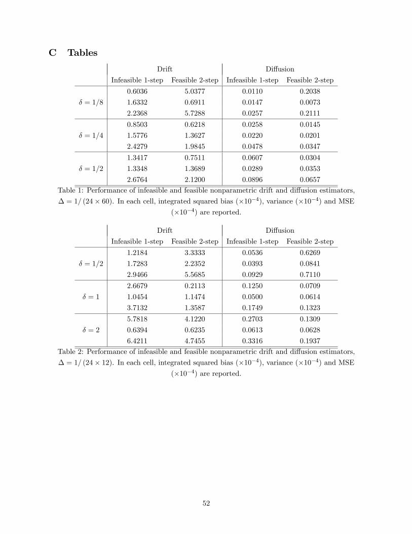
C Tables

Drift Diffusion

Infeasible 1-step Feasible 2-step Infeasible 1-step Feasible 2-step

0.6036 5.0377 0.0110 0.2038

δ = 1/8 1.6332 0.6911 0.0147 0.0073

2.2368 5.7288 0.0257 0.2111

0.8503 0.6218 0.0258 0.0145

δ = 1/4 1.5776 1.3627 0.0220 0.0201

2.4279 1.9845 0.0478 0.0347

1.3417 0.7511 0.0607 0.0304

δ = 1/2 1.3348 1.3689 0.0289 0.0353

2.6764 2.1200 0.0896 0.0657

Table 1: Performance of infeasible and feasible nonparametric drift and diffusion estimators,

∆ = 1/ (24× 60). In each cell, integrated squared bias (×10−4), variance (×10−4) and MSE

(×10−4) are reported.

Drift Diffusion

Infeasible 1-step Feasible 2-step Infeasible 1-step Feasible 2-step

1.2184 3.3333 0.0536 0.6269

δ = 1/2 1.7283 2.2352 0.0393 0.0841

2.9466 5.5685 0.0929 0.7110

2.6679 0.2113 0.1250 0.0709

δ = 1 1.0454 1.1474 0.0500 0.0614

3.7132 1.3587 0.1749 0.1323

5.7818 4.1220 0.2703 0.1309

δ = 2 0.6394 0.6235 0.0613 0.0628

6.4211 4.7455 0.3316 0.1937

Table 2: Performance of infeasible and feasible nonparametric drift and diffusion estimators,

∆ = 1/ (24× 12). In each cell, integrated squared bias (×10−4), variance (×10−4) and MSE

(×10−4) are reported.

52

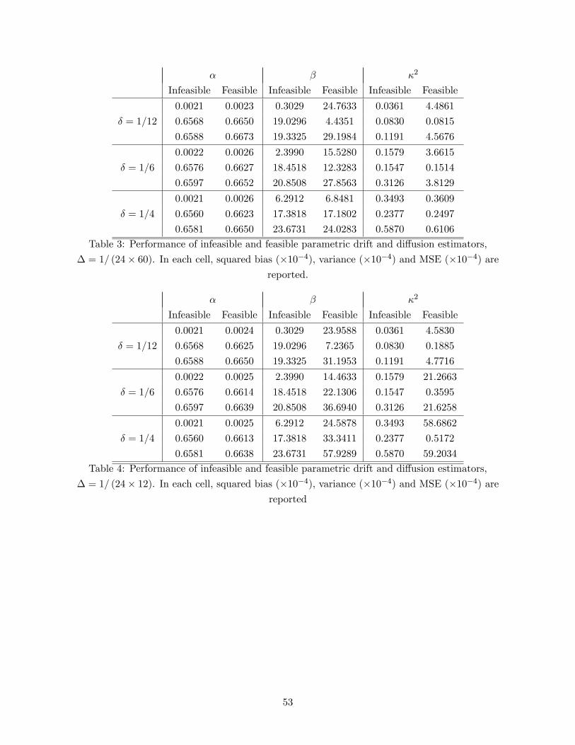
α β κ2

Infeasible Feasible Infeasible Feasible Infeasible Feasible

0.0021 0.0023 0.3029 24.7633 0.0361 4.4861

δ = 1/12 0.6568 0.6650 19.0296 4.4351 0.0830 0.0815

0.6588 0.6673 19.3325 29.1984 0.1191 4.5676

0.0022 0.0026 2.3990 15.5280 0.1579 3.6615

δ = 1/6 0.6576 0.6627 18.4518 12.3283 0.1547 0.1514

0.6597 0.6652 20.8508 27.8563 0.3126 3.8129

0.0021 0.0026 6.2912 6.8481 0.3493 0.3609

δ = 1/4 0.6560 0.6623 17.3818 17.1802 0.2377 0.2497

0.6581 0.6650 23.6731 24.0283 0.5870 0.6106

Table 3: Performance of infeasible and feasible parametric drift and diffusion estimators,

∆ = 1/ (24× 60). In each cell, squared bias (×10−4), variance (×10−4) and MSE (×10−4) are

reported.

α β κ2

Infeasible Feasible Infeasible Feasible Infeasible Feasible

0.0021 0.0024 0.3029 23.9588 0.0361 4.5830

δ = 1/12 0.6568 0.6625 19.0296 7.2365 0.0830 0.1885

0.6588 0.6650 19.3325 31.1953 0.1191 4.7716

0.0022 0.0025 2.3990 14.4633 0.1579 21.2663

δ = 1/6 0.6576 0.6614 18.4518 22.1306 0.1547 0.3595

0.6597 0.6639 20.8508 36.6940 0.3126 21.6258

0.0021 0.0025 6.2912 24.5878 0.3493 58.6862

δ = 1/4 0.6560 0.6613 17.3818 33.3411 0.2377 0.5172

0.6581 0.6638 23.6731 57.9289 0.5870 59.2034

Table 4: Performance of infeasible and feasible parametric drift and diffusion estimators,

∆ = 1/ (24× 12). In each cell, squared bias (×10−4), variance (×10−4) and MSE (×10−4) are

reported

53

D Figures

Figure 1: Infeasible 1-step estimator of α (x), ∆ = 1/ (24× 60) and δ = 1/4.

Figure 2: Feasible 2-step estimator of α (x), ∆ = 1/ (24× 60) and δ = 1/4.

54

Figure 3: Infeasible 1-step estimator of β2 (x), ∆ = 1/ (24× 60) and δ = 1/4.

Figure 4: Feasible 2-step estimator of β2 (x), ∆ = 1/ (24× 60) and δ = 1/4.

E Supplementary Material

We here provide proofs of some technical results, including Lemma D.1 and Theorem 7.1.

Proof of supt∈[0,T ] |Bt| = oa.s.(T1/2 log T ) as T → ∞ (Section 3.3). By the reflection principle

55

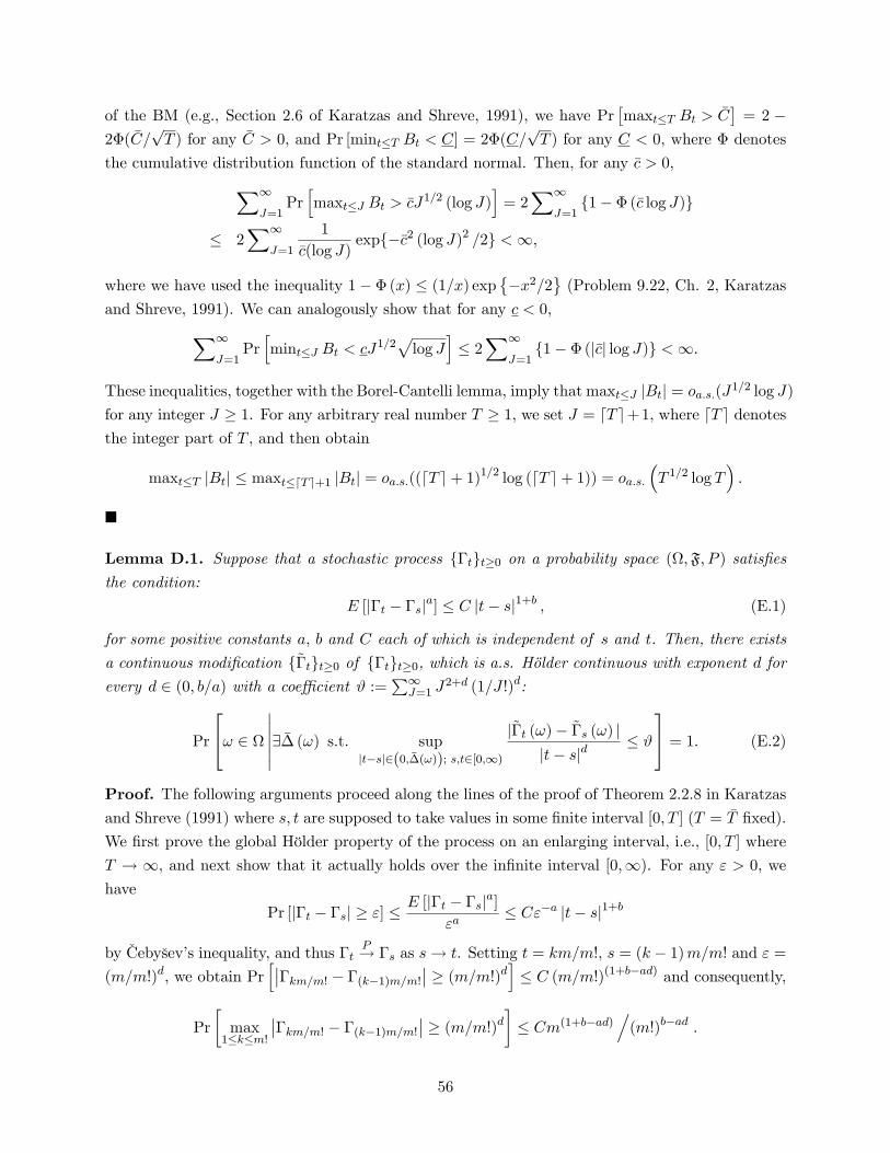
of the BM (e.g., Section 2.6 of Karatzas and Shreve, 1991), we have Pr[maxt≤T Bt > C

]= 2 −

2Φ(C/√T ) for any C > 0, and Pr [mint≤T Bt < C] = 2Φ(C/

√T ) for any C < 0, where Φ denotes

the cumulative distribution function of the standard normal. Then, for any c > 0,∑∞

J=1Pr[maxt≤J Bt > cJ1/2 (log J)

]= 2

∑∞

J=11− Φ (c log J)

≤ 2∑∞

J=1

1

c(log J)exp−c2 (log J)2 /2 <∞,

where we have used the inequality 1− Φ (x) ≤ (1/x) exp−x2/2

(Problem 9.22, Ch. 2, Karatzas

and Shreve, 1991). We can analogously show that for any c < 0,∑∞

J=1Pr[mint≤J Bt < cJ1/2

√log J

]≤ 2

∑∞

J=11− Φ (|c| log J) <∞.

These inequalities, together with the Borel-Cantelli lemma, imply thatmaxt≤J |Bt| = oa.s.(J1/2 log J)

for any integer J ≥ 1. For any arbitrary real number T ≥ 1, we set J = dT e+1, where dT e denotesthe integer part of T , and then obtain

maxt≤T |Bt| ≤ maxt≤dT e+1 |Bt| = oa.s.((dT e+ 1)1/2 log (dT e+ 1)) = oa.s.

(T 1/2 log T

).

Lemma D.1. Suppose that a stochastic process Γtt≥0 on a probability space (Ω,F, P ) satisfies

the condition:

E [|Γt − Γs|a] ≤ C |t− s|1+b , (E.1)

for some positive constants a, b and C each of which is independent of s and t. Then, there exists

a continuous modification Γtt≥0 of Γtt≥0, which is a.s. Hölder continuous with exponent d for

every d ∈ (0, b/a) with a coeffi cient ϑ :=∑∞

J=1 J2+d (1/J !)d:

Pr

ω ∈ Ω

∣∣∣∣∣∣∃∆ (ω) s.t. sup|t−s|∈(0,∆(ω)); s,t∈[0,∞)

|Γt (ω)− Γs (ω) ||t− s|d

≤ ϑ

= 1. (E.2)

Proof. The following arguments proceed along the lines of the proof of Theorem 2.2.8 in Karatzas

and Shreve (1991) where s, t are supposed to take values in some finite interval [0, T ] (T = T fixed).

We first prove the global Hölder property of the process on an enlarging interval, i.e., [0, T ] where

T → ∞, and next show that it actually holds over the infinite interval [0,∞). For any ε > 0, we

have

Pr [|Γt − Γs| ≥ ε] ≤E [|Γt − Γs|a]

εa≤ Cε−a |t− s|1+b

by Cebyšev’s inequality, and thus ΓtP→ Γs as s→ t. Setting t = km/m!, s = (k − 1)m/m! and ε =

(m/m!)d, we obtain Pr[∣∣Γkm/m! − Γ(k−1)m/m!

∣∣ ≥ (m/m!)d]≤ C (m/m!)(1+b−ad) and consequently,

Pr

[max

1≤k≤m!

∣∣Γkm/m! − Γ(k−1)m/m!

∣∣ ≥ (m/m!)d]≤ Cm(1+b−ad)

/(m!)b−ad .

56

By the fact that∑∞

m=1m(1+b−ad)/(m!)b−ad exists and the Borel-Cantelli lemma, there exists a set

Ω∗ ∈ F with Pr (Ω∗) = 1 such that

∀ω ∈ Ω∗, ∃m∗ (ω) , ∀m ≥ m∗ (ω) : max1≤k≤m!

∣∣Γkm/m! − Γ(k−1)m/m!

∣∣ < (m/m!)d (E.3)

, where m∗ is a positive and integer-valued random variable. For each integer m (≥ 1) and any

integer l ≥ m, consider the following sets, Eml := km/l! | k = 0, 1, . . . , l! and Em :=⋃∞l=1E

ml .

The set Eml consists of (l! + 1) points in [0,m], while Em consists of infinitely many points in [0,m].

Note that Em is dense in [0,m] for any m. Now fix ω (∈ Ω∗) and m (≥ m∗ (ω)). We shall show that

∀l > m, ∀t, s ∈ Eml with |t− s| ∈ (0,m/m!) : |Γt (ω)− Γs (ω)| ≤ 2

l∑J=m+1

J2 [J + 1/ ((J + 1)!)]d .

(E.4)

To show this, we use the inductive method. First, we prove that the claim is true for l = m + 1.

For any s, t ∈ Emm+1 with |t− s| ∈ (0,m/m!), there exist some k1, k2 ∈ 0, 1, . . . , (m+ 1)! with0 ≤ k2 − k1 ≤ m such that

|Γt (ω)− Γs (ω)| ≤∣∣Γk1(m+1)/(m+1)! (ω)− Γ(k1+1)(m+1)/(m+1)! (ω)

∣∣+∣∣Γ(k1+1)(m+1)/(m+1)! (ω)− Γ(k1+2)(m+1)/(m+1)! (ω)

∣∣+ · · ·+

∣∣Γ(k2−1)(m+1)/(m+1)! (ω)− Γk2(m+1)/(m+1)! (ω)∣∣ .

Each term on the right-hand side is bounded by m [(m+ 2) / (m+ 2)!]d, which is implied by

the fact Emm+1 ⊂ Em+2m+2 and the inequality eq. (E.3). Thus, by the triangle inequalities, we

have |Γt (ω)− Γs (ω)| ≤ m2 [(m+ 2) / (m+ 2)!]d. Second, suppose that eq. (E.4) is valid for

l = m + 1, . . . , L − 1. For s < t, (s, t ∈ EmL ) with |t− s| ∈ (0,m/m!), consider the num-

bers s1 := minu ∈ EmL−1 : u ≥ s

and t1 := max

u ∈ EmL−1 : u ≤ t

, and notice that s1, t1 ∈

EmL−1 ⊂ EmL ⊂ EL+1L+1 ; s, t ∈ EmL ⊂ EL+1

L+1 ; s1 − s < m/ (L− 1)!; and t − t1 < m/ (L− 1)!.

By the inequality eq. (E.3) with m = L + 1, |Γs1 (ω)− Γs (ω)| ≤ mL ((L+ 1) / (L+ 1)!)d and

|Γt (ω)− Γt1 (ω)| ≤ mL ((L+ 1) / (L+ 1)!)d. There are two possible relationships among s, t, s1

and t1: (i) if |t− s| ≥ m/ (L− 1)!, it holds that s ≤ s1 ≤ t1 ≤ t (with at least one inequality strict);(ii) if |t− s| < m/ (L− 1)!, either of |t− s| < |s1 − t1| = m/ (L− 1)! or |s1 − t1| = 0. Thus, we

have |t1 − s1| ≤ max m/ (L− 1)!, |t− s| ≤ m/m!, and use the induction assumption (E.4) with

l = L− 1:

|Γt1 (ω)− Γs1 (ω)| ≤ 2

L−1∑J=m+1

J2

[J + 1

(J + 1)!

]d. (E.5)

Therefore,

|Γt (ω)− Γs (ω)| ≤ 2mL ((L+ 1) / (L+ 1)!)d + 2L−1∑

J=m+1

J2

[J + 1

(J + 1)!

]d< 2

L∑J=m+1

J2

[J + 1

(J + 1)!

]d.

We have shown eq. (E.4) for any l (> m), as desired.

We can now show that Γt (ω) | t ∈ Em is uniformly Hölder in t for ∀ω ∈ Ω∗ for anym. Consider

any numbers s, t ∈ Em with m ≥ m∗ (= m∗ (ω)) and |t− s| < ∆ (ω) ≡ m∗/m∗!. Note that

57

Em ⊆ Em′ form ≤ m′. We can pick somem′ (≥ m) such that s, t ∈ Em′ with (m′ + 2) / (m′ + 2)! ≤t− s < (m′ + 1) / (m′ + 1)!. Then, by eq. (E.4), we obtain

|Γt (ω)− Γs (ω)| ≤ 2

∞∑J=m′+1

J2

[J + 1

(J + 1)!

]d≤[(m′ + 2

)/(m′ + 2

)!]d × ∞∑

J=1

J2+d (1/J !)d

and thus, |Γt (ω)− Γs (ω)|/ |t− s|d ≤ ch where ϑ :=∑∞

J=1 J2+d (1/J !)d. Note that the existence

of ϑ can be checked by d’Alembert’s criterion for any d (> 0).

We define Γtt≥0 as follows. For ω /∈ Ω∗, set Γt (ω) = 0, t ∈ [0,m]. For ω ∈ Ω∗ and t ∈ Em, setΓt (ω) = Γt (ω). For ω ∈ Ω∗ and t ∈ [0,m]∩ (Em)c, choose a sequence sn∞n=1with sn (∈ Em)→ t;

by the uniform continuity and the fact that sn is Cauchy, Γsn (ω)∞n=1 is also Cauchy, whose limit

depends of t but not on the particular sequence sn; and thus let Γt (ω) = limsn→t Γsn (ω). Thus,

the resulting process Γtt∈[0,m] is continuous, and is also uniformly Hölder in t ∈ [0,m]. We will

show Γt is a modification of Γt: observe that for t ∈ Em, Γt = Γt a.s.; for t ∈ [0,m] ∩ (Em)c

and sn with sn (∈ Em) → t, we have Γsn → Γt in probability (by eq. (E.1)) and Γsn → Γt a.s.,

which implies Γt = Γt a.s.

Let m = [T ] + 1 with [T ] denoting the largest integer less than or equal to T . Now, we have

proved that for any ω ∈ Ω∗, there exist some m∗ (ω) and ∆ (ω) (≡ m∗/m∗!) such that ∀m ≥ m∗ (ω)

sup|t−s|∈(0,∆(ω))

t,s∈[0,T ]

∣∣∣Γt (ω)− Γs (ω)∣∣∣/ |t− s|d ≤ sup

|t−s|∈(0,∆(ω))t,s∈[0,m]

∣∣∣Γt (ω)− Γs (ω)∣∣∣/ |t− s|d ≤ ϑ,

which implies that Pr (Ω1) = 1, where

Ω1 :=

∃∆ (ω) , ∃T ∗, ∀T (≥ T ∗) , sup|t−s|∈(0,∆(ω)); s,t∈[0,T ]

|Γt(ω)−Γs(ω)||t−s|d ≤ ϑ

. (E.6)

Note that

Ω1 ⊂

∃∆ (ω) , ∃T ∗, sup|t−s|∈(0,∆(ω)); s,t∈[0,T ∗]

|Γt(ω)−Γs(ω)||t−s|d ≤ ϑ

=

∃∆ (ω) , ∃T ∗, ∀T (≤ T∗) , sup|t−s|∈(0,∆(ω)); s,t∈[0,T ]

|Γt(ω)−Γs(ω)||t−s|d ≤ ϑ

=: Ω2. (E.7)

Since Pr (Ω1) = 1, we then have Pr (Ω2) = 1. For any events E,F ∈ F, we have the inequality:Pr (E ∩ F ) ≥ Pr (E) + Pr (F )− 1. With E = Ω1 and F = Ω2, we obtain Pr (Ω1 ∩ Ω2) = 1, which,

together with

Ω1 ∩ Ω2 =

ω ∈ Ω

∣∣∣∣∣∣∃∆ (ω) , ∀T, sup|t−s|∈(0,∆(ω)); s,t∈[0,T ]

|Γt(ω)−Γs(ω)||t−s|d ≤ ϑ

,

implies the desired result, eq. (E.2).

58

Proof of Theorem 7.1. Let

U1 (j) : = 2∂θ1α(σ2τ j ; θ

∗1)[α(σ2

τ j ; θ∗1)δ − (σ2

τ j+1 − σ2τ j )]

;

U2 (j) : = 2∂θ2β2(σ2

τ j ; θ∗2)[β2(σ2

τ j ; θ∗2)δ − (σ2

τ j+1 − σ2τ j )

2].

Then, we can then write

Sk(θ∗k, σ

2) = T−1∑N−1

j=1Uk (j) and

H∗−1k E

[Sk(θ

∗k, σ

2)Sk(θ∗k, σ

2)F]H∗−1k = BθkB

Fθk

+ Vθk + Cθk ,

where

Bθk : = −H∗−1k E

[Sk(θ∗k, σ

2)]

;

Vθk : = H∗−1k

(T−2

∑N−1

j=1E[(Uk (j)− E [Uk (j)]) (Uk (j)− E [Uk (j)])F

])H∗−1k ;

Cθk : = H∗−1k

(T−2

∑1≤i 6=j≤N−1

E[(Uk (i)− E [Uk (i)]) (Uk (j)− E [Uk (j)])F

])H∗−1k .

We below provide the proof for part (i) (k = 1) only. Part (ii) (k = 2) can be proved in the same

way, and its proof is omitted. Let L be the differential operator defined by Lf (x) = f ′ (x)α (x) +

f ′′ (x)β2 (x) /2 for any twice differentiable function f . We first consider the expression of Bθ1 :

E [Uk (j)] = −δ2E[∂θ1α(σ2

u; θ∗1)Lα(σ2u

)]+ 2

∫ τ j+1

τ j

∫ s

τ j

∫ u

τ j

E[L∂θ1α(σ2

v; θ∗1)Lα

(σ2u

)]dvduds

= −δ2E[∂θ1α(σ2

t ; θ∗1)Lα

(σ2t

)][1 +O (δ)] , (E.8)

uniformly over j, where we have applied the martingale property of stochastic integrals and Ito’s

lemma to α(σ2s

)− α(σ2

τ j ) and ∂θ1α(σ2u; θ∗1)− ∂θ1α(σ2

τ j ; θ∗1), and the last equality holds since

E[L∂θ1α(σ2

v; θ∗1)Lα

(σ2u

)]≤E[∣∣L∂θ1α(σ2

v; θ∗1)∣∣2]E [∣∣Lα (σ2

u

)∣∣2]1/2≤ E

[∣∣ψ (σ2t

)∣∣4] = O (1) ,

uniformly over any u and v, which follows from the moment conditions in Assumption C-SDR.

Now, the above definition of Bθk and eq. (E.8) implies eq. (7.3) of the main text. To find theexpression of Vθk , first note that

E[U1 (j)U1 (j)F

]= 4E

[∂θ1α(σ2

t ; θ∗1)∂θ1α(σ2

t ; θ∗1)F

×α2(σ2

τ j )δ2 − 2α(σ2

τ j )δ

(∫ τ j+1

τ j

α(σ2s

)ds+

∫ τ j+1

τ j

β(σ2s

)dZs

)

+2

∫ τ j+1

τ j

(∫ s

τ j

α(σ2u)du+

∫ s

τ j

β(σ2u)dZu

)α(σ2

s)ds

+2

∫ τ j+1

τ j

(∫ s

τ j

α(σ2u)du+

∫ s

τ j

β(σ2u)dZu

)β(σ2

s)dZs +

∫ τ j+1

τ j

β2(σ2s)ds

]= δE

[∂θ1α(σ2

t ; θ∗1)∂θ1α(σ2

t ; θ∗1)Fβ2

(σ2t

)]︸ ︷︷ ︸=Ω∗1

[1 +O (δ)] , uniformly over j

59

where Ito’s lemma is applied to (σ2τ j+1 − σ

2τ j )

2 in the first equality; and the second equality follows

from arguments similar to those in deriving eq. (E.8). By the definition of Vθk and the result thatE [Uk (j)] = O

(δ2)uniformly over j,

Vθk = H∗−1k

(T−2

∑N−1

j=1

[δΩ∗1 [1 + o (1)]−O

(δ4)])

H∗−1k = T−1H∗−1

k Ω∗1H∗−1k [1 +O (δ)] ,

as claimed. To find the expression of Cθk , we write

∂θ1α(σ2τ j ; θ

∗1

)[α(σ2

τ j ; θ∗1)δ − (σ2

τ j+1 − σ2τ j )] =: Υ1 (j) + Υ2 (j) ,

where Υ1 (j) := −∂θ1α(σ2τ j ; θ

∗1

) ∫ τ j+1τ j

∫ sτ jLα(σ2u

)duds and

Υ2 (j) := ∂θ1α(σ2τ j ; θ

∗1

)∫ τ j+1

τ j

∫ s

τ j

α′(σ2u

)β(σ2u

)dZuds−

∫ τ j+1

τ j

β(σ2s

)dZs

.

Then, by the martingale property of stochastic integrals, Fubini’s theorem and the conditions in (C-

SDR), E[Υ1 (i) Υ2 (j)F

]= 0 and E

[Υ2 (i) Υ2 (j)F

]= 0 for i 6= j. Given the moment conditions

in (C-SDR), we can show that E[Υ1 (i) Υ1 (j)F

]= O

(δ4)uniformly over any i 6= j, by using

arguments analogous to those for Bθk and Vθk . This, together with eq. (E.8),

E[(Uk (i)− E [Uk (i)]) (Uk (j)− E [Uk (j)])F

]= E[Υ1 (i) Υ1 (j)F]−E [Uk (i)]E [Uk (j)]F = O

(δ4),

which, together with the definition of Cθk , implies that Cθk = O(δ2). This completes the proof.

60