ESTIMATION OF SPEED OF SOUND

USING MEDICAL ULTRASOUND IMAGE

DECONVOLUTION

H.-C. Shin, R. W. Prager,

W. H. Gomersall, N. G. Kingsbury,

G. M. Treece and A. H. Gee

CUED / F-INFENG / TR 626

03 April 2009

Department of Engineering

University of Cambridge

Trumpington Street

Cambridge, CB2 1PZ

United Kingdom

Email:

hs338/rwp/whg21/ngk/gmt11/ahg@eng.cam.ac.uk

Estimation of Speed of Sound using Medical

Ultrasound Image Deconvolution

Ho-Chul Shin, Richard Prager, Henry Gomersall,

Nick Kingsbury, Graham Treece and Andrew Gee

Department of Engineering, University of Cambridge,

Trumpington Street, Cambridge, CB2 1PZ, United Kingdom

Abstract

In diagnostic ultrasound imaging the speed of sound is assumed to be 1540 m/s in soft

tissues. When the actual speed is different, the mismatch can lead to distortions in the

acquired images, and so reduce their clinical value. Therefore, the estimation of the true

speed has been pursued not only because it enables image correction but also as a way of

tissue characterisation. In this paper, we present a novel way to measure the average speed of

sound concurrently with performing image enhancement by deconvolution. This simultaneous

capability, based on a single acquisition of ultrasound data, has not been reported in previous

publications. Our algorithm works by conducting non-blind deconvolution of an ultrasound

image with point-spread functions based on different speeds of sound. Using a search strategy,

we select the speed that produces the best-possible restoration. Deconvolution allows the use

of ultrasound imaging machines almost without modification unlike most other estimation

methods. A conventional handling of a transducer array is all that is required in the data

acquisition part of our proposed method: the data can be collected freehand. We have tested

our algorithm with simulations, in vitro phantoms with known and unknown speeds, and an in

vivo scan. The estimation error was found to be +0.01 ± 0.60 % (mean ± standard deviation)

for in vitro in-house phantoms whose speeds were also measured independently. In addition to

the speed estimation, our method has also proved to be capable of simultaneously producing a

better restoration of ultrasound images than deconvolution by an assumed speed of 1540 m/s,

when this assumption is incorrect.

Keywords: Medical ultrasound image; Non-blind deconvolution; Point-spread function; Dual-

tree complex wavelet transform; Speed of sound; Sound estimation.

1 Introduction

Conventional ultrasound imaging assumes the speed of sound is 1540 m/s in soft tissue for the

design of the beamforming delay pattern. This potentially leads to errors in B-mode images and

in images restored by non-blind deconvolution when the actual speed of sound is different. The

1

effects of errors in the sound speed, such as degraded spatial resolution, have been widely reported,

and some of the consequences have been quantified [1].

Research on the speed of sound in the medical ultrasound community has mainly focused on

two aspects: estimation (in the context of tissue characterisation) and correction (in the context of

image perception). In most previous publications, both topics have been dealt with separately. In

this article, we propose a method of measuring an average speed of sound in broadly homogeneous

tissue with simultaneous image correction if the estimated speed is different from 1540 m/s. We

present this algorithm in a framework of ultrasound image deconvolution [2, 3, 4]. Therefore, our

approach to speed correction in the restored ultrasound images is different from the techniques

employed previously in the original B-mode images.

1.1 Literature survey

Initially, the speed of medical ultrasound was estimated using transmission methods, which mea-

sured the time taken while a pulse propagated between a transmitter and a receiver. Clinical

applications were limited to the breast [5]. Robinson et al. [6] carried out an extensive review of

pulse-echo sound-speed estimation techniques. Nine methods in three categories were examined in

detail. Despite using pulse-echo techniques, most of the reviewed methods were designed to em-

ploy multiple apertures of ultrasound transducers: one for transmission and the rest for reception,

and the use of paired transducer apertures increased the system complexity. A precise geometric

relation needs to be established between transducers and scanned regions of interest [6], and this

is vulnerable to estimation errors. In some methods [6], a pair of crystal elements in a single linear

array can replace a pair of transducer apertures, which however may suffer a low signal-to-noise

ratio. Several methods in [6] were also limited to tissues which have recognisable features in order

to have a geometric relation well-defined. However, there were a couple of methods which worked

using a single transducer aperture. The transaxial compression technique [6, 7] is among them,

but it involves a precise movement of a transducer which compresses the tissue surface plus the

acquisition of multiple scans after compression. In another technique called the dynamic focus

method ([5], p.637 in [6]), the speed of sound in the ultrasonic beamformer is varied by operators

until the clearest image is obtained, which is not systematic and effectively requires multiple scans.

Anderson and Trahey [8] estimated the average speed of sound in a homogeneous medium based

on the quadratic best-fit of the one-way geometric delay pattern acquired on individual elements

of a transducer array. Their method is closely related to those used in exploration seismology and

only requires a single scan of a medium with a single transducer array. Its accuracy and precision

are cited in later sections for comparison purposes with our approach. Later, such a time-delay

pattern was exploited by Pereira et al. [9] with application to bovine livers, but an additional

hydrophone was required as a receiver. Recently, an image registration technique was explored

to estimate the speed of sound [10]. A single transducer array was used, but multiple scans were

necessary following beam steering.

Most of the methods reviewed by Robinson et al. [6] produce the average speed of sound in

the scanned tissues. Only a handful of them were capable of local speed estimation, and the

demonstration of a mapping capability was very rare. Kondo et al. [11] reported mapping of

in vivo local sound-speed estimation. But, they conceded that an exact measurement of local

sound speed was difficult. Recently, a detailed local sound-speed mapping of biological tissue was

2

demonstrated using ultrasound [12]. However, this method using a scanning acoustic microscope

(SAM) is effectively a different modality from that with which we are concerned in this article. The

signal carrier frequency of their system reaches as high as 500 MHz, and as in other microscope

techniques, a non-invasive in vivo measurement is not possible.

Another ultrasound modality using the computed tomography (CT) has also been employed in

mapping the sound speed [13, 14, 15, 16, 17]. In a recent pre-clinical trial [17], a prototype trans-

mission ultrasound CT system was used to image a breast placed in a temperature-controlled water

bath. Transmitter and receiver arrays are rotated around 360◦ to collect 180 sets of tomographic

ultrasound data. The algorithm is based on full-wave non-linear inverse-scattering tomography [16]

and enables the detailed estimation of sound speed as well as attenuation in breast tissue. It demon-

strates the potential use of these acoustic properties in diagnostic breast imaging [17]. However,

the transmissional use of ultrasound in a computed tomographic modality is different from the

pulse-echo approach proposed in this paper and requires higher system complexity.

There is not much literature that describes a perceptual improvement in images associated with

estimating the speed of sound. Napolitano et al. [18] showed the B-mode images of in vitro and

in vivo scans after estimation and subsequent correction of the speed. Although they proposed

an automated algorithm (unlike the operator-dependent method in [5]) by analysing the spatial

frequency information in a B-mode image, the estimation was carried out by acquiring many images

with various trial sound speeds. This was achieved by adjusting the beamformer time delays in

the ultrasound machine.

The correction of wrong acoustic speed effects, especially due to inhomogeneity of tissues, has

been addressed via the correction of phase aberration in medical ultrasound images [8]. Numerous

methods have been proposed [19, 20, 21, 22]. They differ from one another in how they estimate

the aberration profile across the transducer elements, but most of them share the idea of changing

the time delays in individual elements according to the estimated aberration profile. During the

profile estimation process, many techniques require multiple acquisitions of the radio-frequency

(RF) signal. Most of all, previous work on phase aberration has focused on the reduction of

perceived image degradation.

In the category of medical ultrasound image restoration, uncertainty in the speed of sound

especially for in vivo applications may be addressed through blind deconvolution [23, 24, 25, 26,

27, 28], in which a point-spread function (PSF) based on an actual speed of sound is estimated

directly from the image to be restored. However, blind approaches are not used to estimate the

speed of sound because it is not easily parameterised. In contrast, non-blind deconvolution can

make such an estimation possible due to the parameterisation of the sound speed in the PSF.

Our research group has recently studied the effects of uncertainty in the PSF on non-blind

deconvolution [4]. The parameters of an ultrasound imaging PSF have been systematically in-

vestigated. In total, six parameters were examined: uncertainty in the ultrasound machine was

analysed by varying the axial depth of lateral focus and the radius of elevational focus alongside

the height and width of the transducer elements. Sensitivity to tissue influence was investigated

by varying the speed of sound and frequency-dependent attenuation. When the restoration re-

sults were judged visually, we discovered that the two most critical parameters for two-dimensional

deconvolution are the lateral focus and the speed of sound. As far as human perception is con-

cerned, we concluded that it is possible to restore in vivo ultrasound images using an assumed

3

PSF when its error is not significant. However, when the deconvolution results were quantified, we

also proved that there are always differences between restored images from various PSFs, which

human perception may be insensitive to, but which are identifiable through other metrics such as

improvement in the signal-to-noise ratio (ISNR) or correlation. In this article, we will exploit such

differences to estimate a PSF parameter which is the speed of sound in this case.

We briefly introduce our non-blind deconvolution algorithm in Section 2. The proposed estima-

tion method for the speed of sound is explained in Section 3. Subsequently, the applications of the

technique are featured in Section 4 (simulation), Section 5 (in vitro experiments), and Section 6

(in vivo scan). Discussions follow on our proposed technique in Section 7. Finally, conclusions are

drawn.

2 Deconvolution Algorithm

The paper is mainly concerned with the estimation of the sound speed in medical ultrasound

applications. But, the deconvolution of an ultrasound image is a pivotal part of our estimation

process, and is also an important outcome.

When using transducer array probes, the lateral focus is created by a delay profile across the

active aperture. But each calculated depth for lateral focus is only valid when the sound speed is

known and constant. Such an ideal scenario does not usually occur in real clinical scans, resulting

in worse lateral resolution and elevated off-axis response.

Such symptoms have been previously exploited in the estimation of the sound speed [5, 18],

where the delay profiles were repeatedly adjusted until the clearest images were achieved. By

using non-blind deconvolution, these symptoms can be explored but with simpler data acquisition.

Instead of adjusting the delay pattern for multiple image acquisitions, the non-blind deconvolution

enables the use of a single ultrasound scan. The necessary change is carried out off-line only in the

sound speed of a PSF. The comparison of numerous PSFs is conducted through the deconvolution

to figure out which PSF best suits the ultrasound image of interest and hence produces the clearest

restored image. The sound speed used for the best PSF is our estimation of the speed. The metric

to determine such best PSF is explained in Section 3.1.

Because of its importance in our approach, we begin by briefly recapitulating the key compo-

nents of our deconvolution algorithm for the benefit of readers who may not be familiar with it.

Complete details can be found in previous publications [2, 3].

2.1 Ultrasound image formation

The A-lines of an ultrasound imaging system can be mathematically modelled as a Fredholm inte-

gral of the first kind [2]. The wave propagation is assumed linear. Although non-linearity is present

in in vivo scans of clinical applications, our approach is still applicable to ultrasound images when

dominated by linearity. In medical ultrasound imaging, linearity is generally preserved in pulse

propagation and reflection, with higher order harmonic imaging as exceptions [25]. Without loss of

generality, if we adopt a discrete space-time formulation, the integral can be further simplified using

a vector-matrix notation with a complex random variable x as the field of scatterers (or reflectivity

4

function) and y as the complex analytic baseband counterpart of the measured ultrasound signal.

y = H x + n (1)

Potential measurement errors are taken into account as complex additive white Gaussian noise

(n). H is a block diagonal matrix along the lateral and elevational‡ dimensions. Each block

matrix maps from the axial depth dimension to the time domain at a given lateral and elevational

position. Here, multi-dimensional data (y,x,n) are rearranged into one-dimensional equivalents

by lexicographic ordering, and thus the sizes of the vectors and the matrix are: N × 1 for x, n,

and y, and N × N for H. Here, N is the total image size.

In traditional deconvolution algorithms including blind approaches, a blurring function is usu-

ally assumed to be spatially shift invariant. This tends to be true along the lateral and elevational

dimension of an ultrasound image, but the blurring function is significantly shift dependent in the

axial-depth direction. Our deconvolution algorithm is therefore designed to be capable of dealing

with the blurring operator (H) as spatially shift dependent in the axial direction and shift invariant

along the lateral and elevational dimensions [2].

2.2 Deconvolution under an EM framework

Our goal is to estimate a scatterer field x from a noisy and blurred image y. The algorithm

operates in a Bayesian context. Because the finite resolution cell of a PSF merges the responses

from neighbouring scatterers during the blurring process (H x), the deblurring procedure tends to

be ill-posed, and therefore a direct inverse approach is likely to fail. One of the standard solutions

to this problem is to incorporate regularisation in a maximum a posteriori framework (MAP, see

p.314 in [29]) with a prior on the scatterer field.

x = arg maxx

[

ln p(y | x, σ2n) + ln p(x)

]

(2)

Here, x is an estimate of the scatterer field, obtained from the deconvolution process, and σ2n

the variance of n. Possible priors could involve assuming Gaussian or Laplacian statistics for the

scatterer field. The Gaussian prior, in particular, leads to the well-known Wiener filter.

x = arg minx

[

1

2σ2n

‖y − H x‖2 +1

2xHC−1

x x

]

= (HHH + σ2nC−1

x )−1HHy (3)

In a further simplified case of Cx = σ2xIN , this is known as zero-order Tikhonov regularisation. The

superscript H denotes the Hermitian transpose. The term Cx represents the covariance matrix

E(xxH) of the complex random variable x, σ2x the variance of x, and IN the identity matrix with

size N . Instead of using this conventional prior for the entire tissue (x), we model the tissue

reflectivity as the product of microscopically randomised fluctuations (w) and a macroscopically

smooth tissue-type image called the echogenicity map (S) which shares the characteristics of natural

images [3].

x = S w (4)

‡The elevational dimension is included for the complete general formulation, even though the two-dimensionalultrasound images of the axial and lateral directions are the main concern in this article.

5

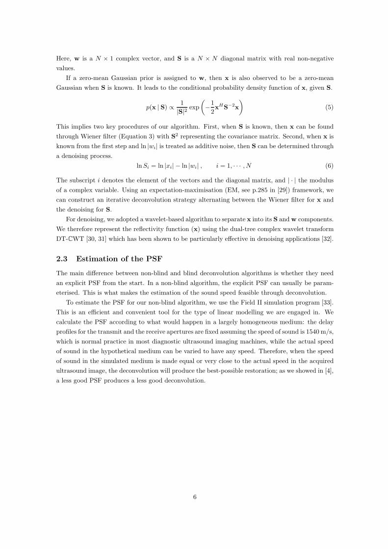
Here, w is a N × 1 complex vector, and S is a N × N diagonal matrix with real non-negative

values.

If a zero-mean Gaussian prior is assigned to w, then x is also observed to be a zero-mean

Gaussian when S is known. It leads to the conditional probability density function of x, given S.

p(x | S) ∝1

|S|2exp

(

−1

2xHS−2x

)

(5)

This implies two key procedures of our algorithm. First, when S is known, then x can be found

through Wiener filter (Equation 3) with S2 representing the covariance matrix. Second, when x is

known from the first step and ln |wi| is treated as additive noise, then S can be determined through

a denoising process.

lnSi = ln |xi| − ln |wi| , i = 1, · · · , N (6)

The subscript i denotes the element of the vectors and the diagonal matrix, and | · | the modulus

of a complex variable. Using an expectation-maximisation (EM, see p.285 in [29]) framework, we

can construct an iterative deconvolution strategy alternating between the Wiener filter for x and

the denoising for S.

For denoising, we adopted a wavelet-based algorithm to separate x into its S and w components.

We therefore represent the reflectivity function (x) using the dual-tree complex wavelet transform

DT-CWT [30, 31] which has been shown to be particularly effective in denoising applications [32].

2.3 Estimation of the PSF

The main difference between non-blind and blind deconvolution algorithms is whether they need

an explicit PSF from the start. In a non-blind algorithm, the explicit PSF can usually be param-

eterised. This is what makes the estimation of the sound speed feasible through deconvolution.

To estimate the PSF for our non-blind algorithm, we use the Field II simulation program [33].

This is an efficient and convenient tool for the type of linear modelling we are engaged in. We

calculate the PSF according to what would happen in a largely homogeneous medium: the delay

profiles for the transmit and the receive apertures are fixed assuming the speed of sound is 1540 m/s,

which is normal practice in most diagnostic ultrasound imaging machines, while the actual speed

of sound in the hypothetical medium can be varied to have any speed. Therefore, when the speed

of sound in the simulated medium is made equal or very close to the actual speed in the acquired

ultrasound image, the deconvolution will produce the best-possible restoration; as we showed in [4],

a less good PSF produces a less good deconvolution.

6

3 Method

3.1 Correlation metrics

The overall strategy of our speed estimation method is to run multiple deconvolutions using PSFs

with different speeds and to pick the speed which produces the best restoration. Therefore, a metric

capable of determining the best outcome is as crucial as the non-blind deconvolution algorithm

itself. In a previous paper [4], we showed that the deconvolution result could be quantified, and

demonstrated that the mean correlation length of the restored image is significantly smaller than

that of the original ultrasound image, for example, 0.32 and 0.61 mm, respectively [4]. To this

effect, the autocorrelation was evaluated and the half-energy width of the peak (a.k.a. FWHM)

was measured.

This correlation length worked well for separating the original ultrasound image from its decon-

volved image. However, we found that such a FWHM-based correlation length was not sensitive

enough to distinguish deconvolution results with close PSFs from one another (see Figure 1). A

possible explanation for this failure is that most restorations result in physically smaller speckle

(see deconvolution images in [4]). The FWHM approach depends on only a few lags relating to

neighbouring pixels and so does not take into account the rest of the longer lags. Therefore, once

the speckle (represented by smaller lags in the correlation) was reduced to similar sizes, restorations

with similar PSFs may not be easily discriminated through such a correlation metric.

In addressing this challenge, we subsequently discovered that accounting for all the lags in the

correlation could be more relevant than the FWHM metric. The same autocorrelation (Rxi[l]) is

calculated along the lateral line (xi) at each i-th axial depth as the case for the FWHM metric and

then a summation (∑

l|Rxi

[l]|) is made of the magnitude of all the l coefficients of the correlation.

To produce a single-valued representation, another summation (∑

i

∑

l|Rxi

[l]|) was taken of this

value for all axial depths. During the course of this paper, the correlation metric is evaluated

according to this summation-based strategy.

Figure 1 shows a graph of the aforementioned summation-based correlation metric for various

speeds of sound in a simulated phantom§. The values of the correlation are normalised for display

because the metric itself does not directly indicate a meaningful physical quantity but the relative

differences are most important. The same convention is followed throughout this article. To

produce the data in Figure 1, the PSFs for 49 different speeds were evaluated and the deconvolution

algorithm was run for each of them. The speeds of sound in the plot cover the range from −300 to

+300 m/s (the reference and correct speed being 1540 m/s) in 12.5 m/s steps denoted by discrete

marks. The curves in the graph indicate the correlation metric after different numbers of iterations

in the EM deconvolution algorithm. Increasing the number of iterations is observed to lower the

correlation, which indicates an improved restoration. The result illustrates that the correlation

metric returns the minimum value when the blurred ultrasound image is deconvolved with the

PSF with the correct speed of sound, and demonstrates the possibility of finding such a correct

value.

§The simulation process is explained later in Section 4.

7

−300 −200 −100 0 100 200 3001

1.05

1.1

1.15

1.2

1.25

Cor

rela

tion

met

ric

∆ speed of sound, m/s

−300 −200 −100 0 100 200 3000.3

0.35

0.4

0.45

FW

HM

cor

rela

tion

leng

th,

mm

iter. 1iter. 4iter. 7FWHM

Figure 1: Plot of correlation metrics vs. various speeds of sound in a simulated phantom forexemplar EM iteration stages. The summation-based correlation is normalised by its minimumfor display purposes and its scale is shown on the left. The FWHM-based correlation length forthe 4th EM iteration is shown for comparison and its scale is displayed on the right. The spacingbetween data points is 12.5 m/s, and the reference speed (∆ = 0) is 1540 m/s.

3.2 Iterative method under an EM structure

Perhaps, locating the correct speed of sound may be achieved by resorting to a “brute-force”

approach demonstrated in Section 3.1 and Figure 1. A method reported in [18] effectively adopts

such a strategy. Their core algorithm to determine the correct speed is different from ours, but

they essentially repeat their algorithm for as many different trial speeds as possible. Although

such an approach may be effective, it is not necessarily efficient. Even though the expected range

of speeds is widely known for particular types of tissue, the speed in an abnormal tissue may be

outside this range. A brute-force approach can also be computationally expensive depending on

the resolution between adjacent trial speeds.

The presence of a well-defined distinct minimum in Figure 1 enables us to adopt an optimi-

sation procedure to find the correct speed of sound. We implemented a gradient-descent based

approach to track down the optimum speed. As demonstrated in the figure, the local minimum

coincides with the global minimum, therefore, we use Newton’s method for the optimisation [34].

First, we start with three initial guesses: three different PSFs defined by three different speeds of

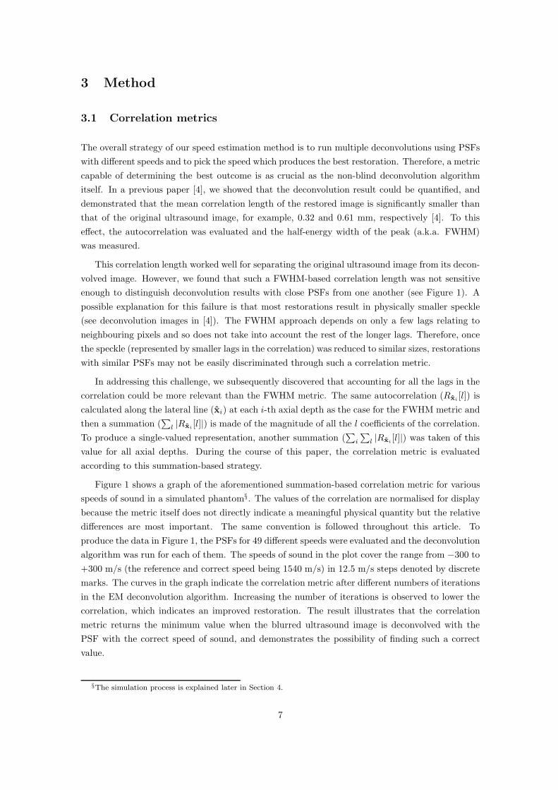
sound. The flow diagram in Figure 2 illustrates the search process. A single iteration of our EM

deconvolution algorithm [3] is carried out with these three PSFs. The correlation metrics of the

three deconvolutions are calculated, and a one-dimensional quadratic equation is formulated based

on the three pairs of sound speeds and corresponding correlation metrics: f(x) = Ax2 + B x + C,

where x is the speed of sound, f(x) the correlation metric, and A, B, C coefficients. Then, the next

search speed is determined from the first and second derivatives of f(x).

xi+1 = xi − αf

′

(xi)

f ′′ (xi)(7)

8

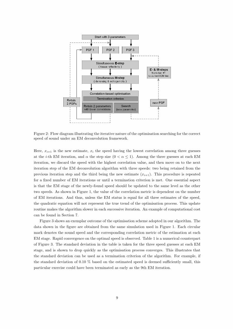
Figure 2: Flow diagram illustrating the iterative nature of the optimisation searching for the correctspeed of sound under an EM deconvolution framework.

Here, xi+1 is the new estimate, xi the speed having the lowest correlation among three guesses

at the i-th EM iteration, and α the step size (0 < α ≤ 1). Among the three guesses at each EM

iteration, we discard the speed with the highest correlation value, and then move on to the next

iteration step of the EM deconvolution algorithm with three speeds: two being retained from the

previous iteration step and the third being the new estimate (xi+1). This procedure is repeated

for a fixed number of EM iterations or until a termination criterion is met. One essential aspect

is that the EM stage of the newly-found speed should be updated to the same level as the other

two speeds. As shown in Figure 1, the value of the correlation metric is dependent on the number

of EM iterations. And thus, unless the EM status is equal for all three estimates of the speed,

the quadratic equation will not represent the true trend of the optimisation process. This update

routine makes the algorithm slower in each successive iteration. An example of computational cost

can be found in Section 7.

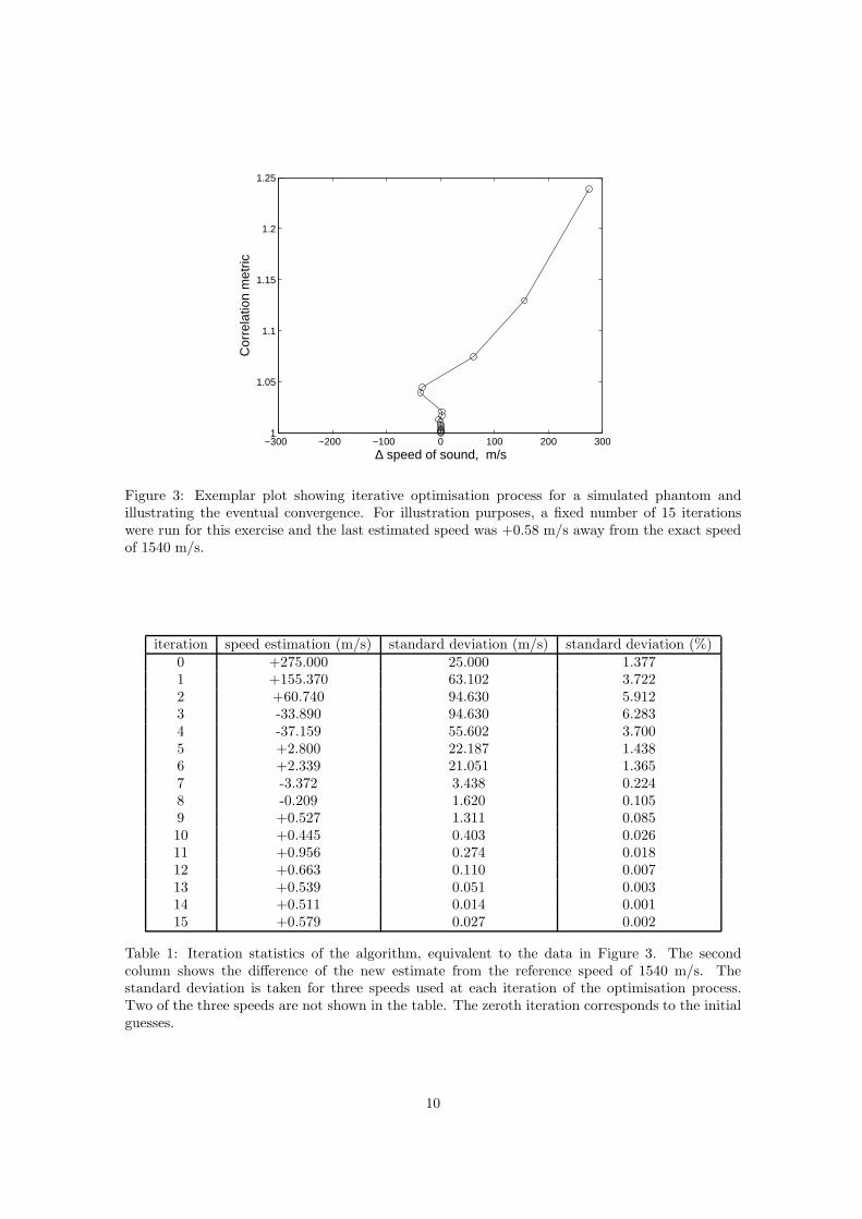
Figure 3 shows an exemplar outcome of the optimisation scheme adopted in our algorithm. The

data shown in the figure are obtained from the same simulation used in Figure 1. Each circular

mark denotes the sound speed and the corresponding correlation metric of the estimation at each

EM stage. Rapid convergence on the optimal speed is observed. Table 1 is a numerical counterpart

of Figure 3. The standard deviation in the table is taken for the three speed guesses at each EM

stage, and is shown to drop quickly as the optimisation process converges. This illustrates that

the standard deviation can be used as a termination criterion of the algorithm. For example, if

the standard deviation of 0.10 % based on the estimated speed is deemed sufficiently small, this

particular exercise could have been terminated as early as the 9th EM iteration.

9

−300 −200 −100 0 100 200 3001

1.05

1.1

1.15

1.2

1.25

∆ speed of sound, m/s

Cor

rela

tion

met

ric

Figure 3: Exemplar plot showing iterative optimisation process for a simulated phantom andillustrating the eventual convergence. For illustration purposes, a fixed number of 15 iterationswere run for this exercise and the last estimated speed was +0.58 m/s away from the exact speedof 1540 m/s.

iteration speed estimation (m/s) standard deviation (m/s) standard deviation (%)0 +275.000 25.000 1.3771 +155.370 63.102 3.7222 +60.740 94.630 5.9123 -33.890 94.630 6.2834 -37.159 55.602 3.7005 +2.800 22.187 1.4386 +2.339 21.051 1.3657 -3.372 3.438 0.2248 -0.209 1.620 0.1059 +0.527 1.311 0.08510 +0.445 0.403 0.02611 +0.956 0.274 0.01812 +0.663 0.110 0.00713 +0.539 0.051 0.00314 +0.511 0.014 0.00115 +0.579 0.027 0.002

Table 1: Iteration statistics of the algorithm, equivalent to the data in Figure 3. The secondcolumn shows the difference of the new estimate from the reference speed of 1540 m/s. Thestandard deviation is taken for three speeds used at each iteration of the optimisation process.Two of the three speeds are not shown in the table. The zeroth iteration corresponds to the initialguesses.

10

4 Simulations

First, we applied our sound-speed estimation technique to a two-dimensional simulated phantom.

The way the simulation was conducted is explained in this section.

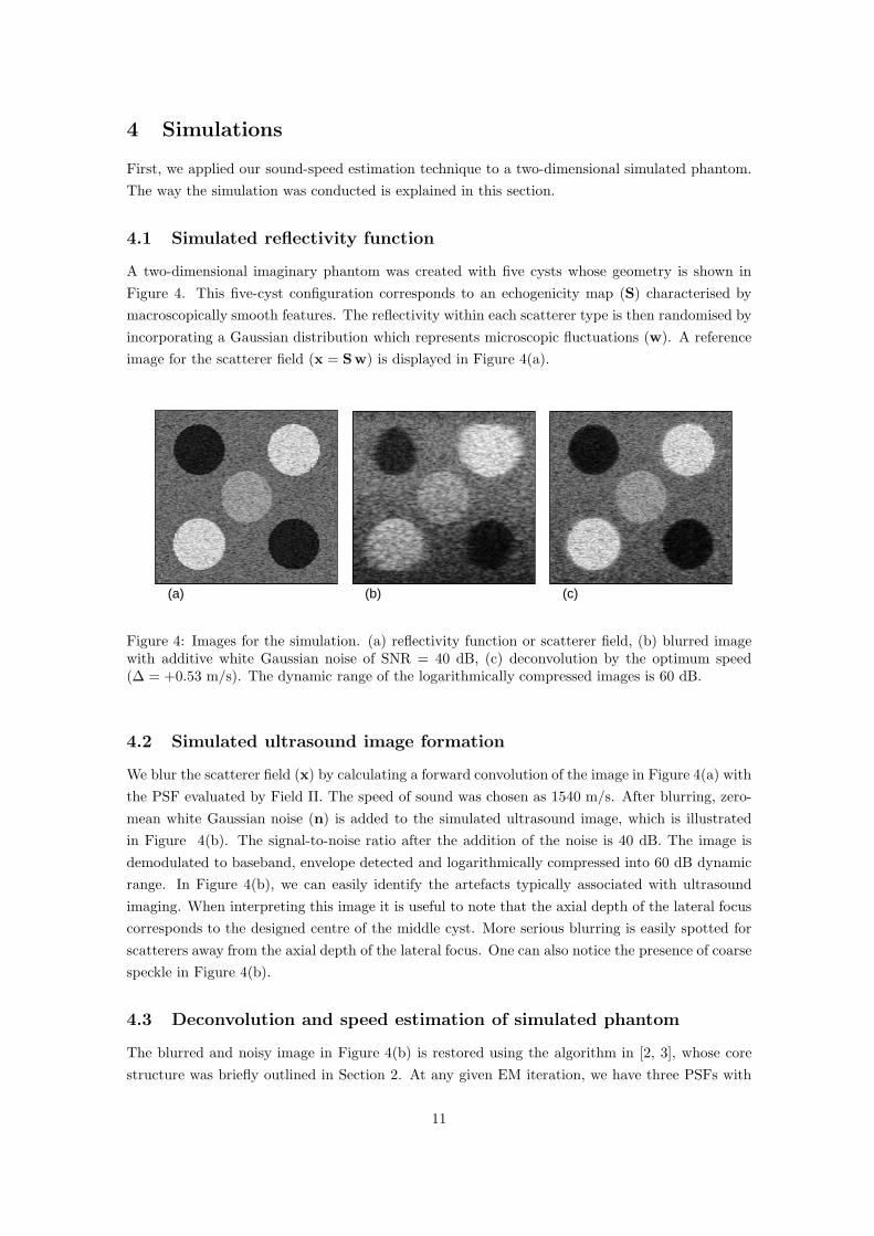
4.1 Simulated reflectivity function

A two-dimensional imaginary phantom was created with five cysts whose geometry is shown in

Figure 4. This five-cyst configuration corresponds to an echogenicity map (S) characterised by

macroscopically smooth features. The reflectivity within each scatterer type is then randomised by

incorporating a Gaussian distribution which represents microscopic fluctuations (w). A reference

image for the scatterer field (x = Sw) is displayed in Figure 4(a).

(a) (b) (c)

Figure 4: Images for the simulation. (a) reflectivity function or scatterer field, (b) blurred imagewith additive white Gaussian noise of SNR = 40 dB, (c) deconvolution by the optimum speed(∆ = +0.53 m/s). The dynamic range of the logarithmically compressed images is 60 dB.

4.2 Simulated ultrasound image formation

We blur the scatterer field (x) by calculating a forward convolution of the image in Figure 4(a) with

the PSF evaluated by Field II. The speed of sound was chosen as 1540 m/s. After blurring, zero-

mean white Gaussian noise (n) is added to the simulated ultrasound image, which is illustrated

in Figure 4(b). The signal-to-noise ratio after the addition of the noise is 40 dB. The image is

demodulated to baseband, envelope detected and logarithmically compressed into 60 dB dynamic

range. In Figure 4(b), we can easily identify the artefacts typically associated with ultrasound

imaging. When interpreting this image it is useful to note that the axial depth of the lateral focus

corresponds to the designed centre of the middle cyst. More serious blurring is easily spotted for

scatterers away from the axial depth of the lateral focus. One can also notice the presence of coarse

speckle in Figure 4(b).

4.3 Deconvolution and speed estimation of simulated phantom

The blurred and noisy image in Figure 4(b) is restored using the algorithm in [2, 3], whose core

structure was briefly outlined in Section 2. At any given EM iteration, we have three PSFs with

11

different speeds of sound, and the deconvolution algorithm is run concurrently for these three

estimations as described in Section 3. Graphs showing correlation metrics and the convergence

pattern have already been introduced in Figures 1 and 3.

An example result of the deconvolution is shown in Figure 4(c). The restored image is the

outcome of our speed estimation process. The estimated sound speed is +0.53 m/s away from the

correct speed of 1540 m/s, when the optimisation process is terminated at the 9th EM iteration

(see Table 1, using the standard deviation of 0.10 % and lower). A high degree of restoration

is observed. The cysts appear again as circles with sharp boundaries. Furthermore, the speckle

size is significantly reduced, but the speckle is retained, which is important because this textural

information can be usefully interpreted in clinical applications.

One may ask why the deconvolved result does not look perceptually the same as the designed

reflectivity function despite the use of almost the same PSF for both forward and backward op-

erations in the simulation. This is because of the presence of the additive Gaussian noise, and

because of the blurring which involves some loss of high frequency information and consequently

causes the deblurring problem to be ill-posed.

5 In vitro measurements

After verifying the operation of our sound-speed estimation technique in the simulation, we pro-

ceeded to apply the estimation algorithm to in vitro data sets. In this section, we present the

results obtained from laboratory phantoms with known and unknown speeds of sound. For the

phantoms of unknown sound speed, we have also conducted independent measurements of their

speeds.

5.1 Measurements on a phantom with a known speed of sound

First, we applied our speed-of-sound estimation method to an in vitro phantom with a known

speed of sound. The phantom has several cysts with back-scattering strengths different from

the background. It was manufactured by the Ultrasound Research Group at the University of

Wisconsin-Madison. The sound speed of the phantom is around 1545 m/s, which is based on

the speed measurements of its components conducted by the manufacturer. Due to some level of

diffusion between adjacent components, there could be uncertainty of approximately ±5 m/s in its

average speed of sound. In addition, no information is available on the temperature dependence

of its sound speed. Therefore, some error in our estimation method could be caused by these

uncertainties. Nonetheless we treat the speed of 1545 m/s as the ground truth for this phantom.

Throughout this article, the following ultrasound system was used to acquire the RF data for

in vitro and in vivo measurements. The system consisted of a General Electric¶ probe RSP6-12

and a Diasus ultrasound machine from Dynamic Imaging Ltd.‖, which was synchronised with a

Gage∗∗ Compuscope CS14200 digitiser. The digitisation process was linked to the locally-developed

Stradwin software††, which is a user-friendly cross-platform tool for medical ultrasound acquisition

and visualisation.

¶GE Healthcare, Pollards Wood, Nightingales Lane, Chalfont St Giles, BUCKS UK‖Dynamic Imaging used to be based near Edinburgh in Scotland, but they are no longer in business.

∗∗Gage, 900 N. State Street, Lockport IL 60441, USA††This is available free at http://mi.eng.cam.ac.uk/˜rwp/stradwin/ .

12

1240 1340 1440 1540 1640 1740 18401

1.02

1.04

1.06

1.08

1.1

1.12

Speed of sound, m/s

Cor

rela

tion

met

ric

iter. 10Optimisation

Figure 5: Exemplar plot showing iterative optimisation process for an in vitro phantom with aknown sound speed of 1545 m/s. The smooth curve was obtained by running the deconvolutionalgorithm with PSFs having 49 different speeds at the 10th EM iteration.

Figure 5 shows a result of the algorithm applied to the known-speed phantom. The speed

estimation of the last 15th iteration is +1.50 m/s away from the speed of 1545 m/s. The smooth

dashed curve in the graph is obtained by running the EM algorithm concurrently for 49 different

speeds of sound as shown in Figure 1. This process of parallel running is not required for our

speed optimisation procedure, but is shown additionally to demonstrate that our optimisation step

does converge to the minimum for an in vitro measurement as well. For this particular exercise,

the estimation error is +0.10 %. We have also conducted estimations for further data sets having

different lateral focus settings and using various sets of initial guesses. The overall estimation error

for this phantom turned out to be −6.82 ± 4.82 m/s (or −0.44 ± 0.31 %) in a notation of “mean

± standard deviation”.

5.2 Measurements on phantoms with unknown speeds of sound

Now we turn our attention to in vitro phantoms with speeds of sound which are not known a

priori .

5.2.1 In-house phantoms

We locally produced ultrasound tissue-mimicking phantoms by mixing agar powder, scatterers and

water [35]. The speed of sound is not known for these in-house phantoms a priori, and hence we

measured it independently of our deconvolution-based estimation method. We applied a time-of-

flight method by measuring the time for sound to travel between known positions. Wires were put

inside phantoms to determine travelling distances. The time-of-flight method was chosen over other

existing techniques because the same ultrasound data can be used for it and our deconvolution-

based method.

13

5.2.2 Time-of-Flight method

Although the time-of-flight method is well established in other branches of medical ultrasound

research [36], it may not have been widely used with multi-element focused pulse-echo ultrasound.

Therefore, we feel that such use in our particular configuration must be validated in order for it to

be used as an independent verification of our deconvolution-based estimation method.

To validate our version of the time-of-flight method, we conducted measurements in deionised

water with stretched wires and compared the speed measurements with published values. For the

time-of-flight technique, we chose an A-line with the least blurring of the target wires. Then,

its envelope was detected with the Hilbert transform and the peaks from the wires were selected

as known reference locations. The distance between wires was taken from their geometric design

but was not actually measured. The travelling time was then worked out from the number of

samples between wire peaks and the sampling rate of 66.67 MHz. Hence, the speed of sound

between the wires is easily estimated. In the literature, the speed of sound in water at various

temperatures and atmospheric pressures has been measured experimentally, and look-up tables

and numerical formulae have been proposed. In distilled water, we use the following simplified

version (Equation 5.22 in [37]) as our reference,

c (PG, t) = 1402.7 + 488t− 482t2 + 135t3 +(

15.9 + 2.8t + 2.4t2)

(PG/100) (8)

where PG is the gauge pressure in bars and t = T/100, with T in degrees Celsius. This equation

is accurate to within 0.05 % for 0 ≤ T ≤ 100◦C and 0 ≤ PG ≤ 200 bar.

We have acquired numerous readings of time-of-flight methods for different lateral focal depths

and wire alignments together with water temperature and atmospheric pressure. The mean tem-

−0.6

−0.4

−0.2

0

0.2

0.4

0.6

Err

or,

%

Lateral focus, mm

9.2

mm

12.

4 m

m

16.

0 m

m

19.

0 m

m

23.

3 m

m

30.

0 m

m

40.

0 m

m

un−

focu

sed

Figure 6: The error associated with the time-of-flight method of measuring the sound speed ofdeionised water. The three different levels of grey at each lateral focal depth indicate different wirealignments: parallel or perpendicular (and mixture of the two) to the B-mode image. The delayprofile for the lateral focus was set assuming a sound speed of 1540 m/s.

14

perature and pressure were 23.0◦C and 1010.3 mb, respectively, which makes a mean sound speed

of 1491.1 m/s according to Equation 8. The comparison of two methods is shown in Figure 6. The

overall error in the chart is +0.14 ± 0.16 %, when the values from Equation 8 are taken as the

ground truth. Perhaps, a trend in error may be noticed in the graph depending on the lateral focal

depth, but the magnitude of errors is found to be as small as those published via other methods

of speed-of-sound estimation. Anderson and Trahey [8] reported the accuracy of their estimation

technique was from +0.08 ± 0.07 % to +0.27 ± 0.05 % for distilled water (see Table 1 in [8]).

Therefore, we concluded that the time-of-flight method is also applicable to our configuration us-

ing pulse-echo focused ultrasound and can be used as an independent validation of our proposed

method in this article.

1240 1340 1440 1540 1640 1740 18401

1.04

1.08

1.12

1.16

1.2

Speed of sound, m/s

Cor

rela

tion

met

ric

0

1

2

3

4

5 ~ 15

iter. 10OptimisationTime−of−Flight

Figure 7: Exemplar plot showing the iterative optimisation process for an in vitro in-house phantomwith an unknown speed of sound. Integers next to circles indicate the iteration numbers, and thezeroth iteration corresponds to one of the initial guesses. The correlation metric obtained at the10th iteration of deconvolution with 49 PSFs is also shown in the smooth dashed curve. The speedwas also independently measured by the time-of-flight method denoted by the vertical dotted line,in which the y-axis value is irrelevant.

5.2.3 Speed-of-sound estimation of in-house phantoms

We have repeated the same set of exercises for the in-house phantoms as for the simulation (Sec-

tion 4) and the known-speed phantom (Section 5.1): finding the correct average speed via the

deconvolution-based optimisation and running multi-speed deconvolution for comparison purpose.

Figure 7 shows an exemplar result obtained from an in vitro in-house phantom measurement. One

interesting aspect of the optimisation curve is that there is a peculiar overshoot in the 4th iteration.

That is because the pairs of speed guesses and corresponding correlation metrics at this iteration

do not conform to our quadratic assumption but rather to a linear formulation having a very small

f′′

(xi) in Equation 7. However, the algorithm is robust enough to correct such odd behaviour.

In the figure, we also show an independent measurement of the sound speed by the time-of-flight

method (the vertical dotted line). The speed estimations for this example are 1455.89 m/s by

15

the deconvolution and 1460.46 m/s by the time-of-flight method. The error is −0.31 % when the

time-of-flight based estimation is taken as a reference.

More RF ultrasound data sets were acquired for in vitro in-house phantoms with various lat-

eral focal depths and different wire alignments. The graphical information is shown in Figure 8

illustrating the estimation errors of our algorithm when the time-of-flight estimations are taken as

the ground truth. The overall estimation error is +0.01 ± 0.60 %. Anderson and Trahey quoted

errors of −0.05 ± 0.44 % and −0.18 ± 0.52 % for phantoms composed of sponge and agar-graphite,

respectively (see Table 1 in [8]).

−2

−1.5

−1

−0.5

0

0.5

1

1.5

Err

or,

%

Lateral focus, mm

9.20

mm

12.4

0 m

m

16.0

0 m

m

19.0

0 m

m

23.3

0 m

m

30.0

0 m

m

40.0

0 m

m

Figure 8: The error associated with the sound-speed estimation for in vitro in-house phantomsusing deconvolution. The reference speeds were those measured by the time-of-flight method. Thefour different levels of grey at each lateral focal depth indicate different wire alignments: parallelor perpendicular (and mixture of the two) to the B-mode image. The delay profile for the lateralfocus was set assuming a sound speed of 1540 m/s.

Previously [4], we analysed the sensitivity of the ultrasound image deconvolution to the pa-

rameters of the PSF. The speed of sound is one of the parameters investigated in the study. It

was discovered that restored images by two different PSFs would be judged differently in human

perception when their parameters were significantly different. The finding served as one of the

motivations in this article: we may be able to produce a restored image better than that decon-

volved by the PSF having the assumed speed of 1540 m/s, when the original ultrasound image was

acquired from tissue having sound speed far away from 1540 m/s. So far, we have demonstrated

that our algorithm is capable of estimating the speed of sound in tissue-mimicking materials. Now,

in Figure 9, we provide the evidence of a further enhanced image by restoration with an optimum

speed of sound. The image in the left panel is the original ultrasound image acquired by an ul-

trasound system whose beamforming delay is set to the sound speed of 1540 m/s. The middle is

the restoration by a correct speed of sound (1455.89 m/s) estimated by our algorithm. The right

is the restored image by the PSF having the speed of 1540 m/s. It is clear that the deconvolution

result via 1540 m/s has smaller speckle sizes and smaller footprint of a wire in the centre than

those of the original image. However, it is observed that the deconvolution image by a correct

16

speed of sound has the best quality: the wire at the centre is restored to its original circular shape,

and speckle in the surrounding area is clearly smaller than that from both the original ultrasound

image and the deconvolution by a nominal speed of 1540 m/s.

Figure 9: Ultrasound images of an in vitro in-house phantom: (left) original ultrasound image,(middle) deconvolution by an optimum speed of 1455.89 m/s, (right) deconvolution by a nominalspeed of 1540 m/s. The size of the images is 14.6 mm × 17.5 mm, when the speed of sound isassumed as 1540 m/s for comparison purposes. The ultrasound data set is the same as that usedin Figure 7. The dynamic range of the logarithmically compressed images is 60 dB. The wire is inthe centre of each image. Note its size changes at each image.

6 In vivo measurements

We have also run our algorithm on an in vivo ultrasound image taken freehand from a human

testicle. The experimental protocol was reviewed by a local ethics committee and informed con-

sent of the subject was obtained. The result showing the convergence of the algorithm is displayed

in Figure 10 which also includes the output of deconvolution with 49 different PSFs for compar-

ison. Our optimisation algorithm converges to the minimum, and the estimated speed of sound

is 1521.37 m/s. The ultrasound images are illustrated in Figure 11. Unlike the stark perceptual

difference noticed in the in vitro phantom of Figure 9, the two restoration images from the middle

(using 1521.37 m/s) and right (using 1540 m/s) windows appear very similar. However it is clear

that both deconvolution solutions are enhanced greatly from the original ultrasound B-scan in the

left panel. The minimal perceptual dissimilarity may be attributed to the fact that the difference

of the speeds used for both deconvolutions is not very large. For example, the speed difference in

the in vitro case in Figure 9 is 84.11 m/s. In contrast, the difference for this in vivo example is

18.63 m/s. Such perceptual insensitivity in Figure 11 due to a small speed difference was also one

of the findings in our previous publication [4].

17

1240 1340 1440 1540 1640 1740 18401

1.01

1.02

1.03

1.04

1.05

1.06

1.07

1.08

Speed of sound, m/s

Cor

rela

tion

met

ric

iter. 10Optimisation

Figure 10: Exemplar plot showing the iterative optimisation process for an in vivo scan of a humantesticle. The correlation metric obtained at the 10th iteration of deconvolution with 49 PSFs isalso shown in the smooth dashed curve.

Figure 11: Ultrasound images of an in vivo human testicle: (left) original ultrasound image,(middle) deconvolution by an optimum speed of 1521.37 m/s, (right) deconvolution by a nominalspeed of 1540 m/s. The size of the images is 14.6 mm × 17.5 mm, when the speed of sound isassumed as 1540 m/s for comparison purposes. The ultrasound data set is the same as that usedin Figure 10. The dynamic range of the logarithmically compressed images is 60 dB.

18

7 Discussions

Although our proposed technique for medical ultrasound speed estimation has several advantages

over other methods reported in previous publications, there are still limitations and room for

further improvement in the approach. Perhaps, the greatest shortcoming of all is its inability

to handle inhomogeneous tissues. In addition, our algorithm is currently not equipped to deal

with the correction of phase aberration which is often created by irregular layers through which

ultrasound travels. There is a potential risk of estimating the speed incorrectly especially in vivo,

where the received RF signals usually have to pass through the human skin interface whose speed

may be different from the rest of the tissue. The situation could be more problematic when the

scanned tissue is indeed heterogeneous or at least multi-layered in its simpler form. In order to

address such a multi-layered soft tissue, the PSF estimated in a lower layer has to be constructed

with a propagation history of the upper tissues. Because the PSF we use in this article assumes

homogeneity, our correlation metric would select a speed of sound whose PSF and consequent

deconvolution would produce the average speed.

In a simple dual layer case of the skin and the remaining largely homogeneous layer, if the

thickness of the skin is much smaller than the area in the rest of the image, then the estimated

average speed of sound could be closer to the main tissue than that of the skin. The fact that the

deconvolved image (for example in Figure 11) is significantly improved from the original B-mode

image may suggest that the PSF used for the restoration is close to the exact but unknown PSF

inherent in the acquired ultrasound image. This is because, in our previous findings [4], we showed

that the image restoration could turn out degraded if the assumed PSF is far away from the true

one.

In a case where the effect of upper layers is not negligible, or in a truly heterogeneous case,

errors are likely to occur. When correlation metrics are plotted at different speeds, there may be

several local minima, or a plateau of minima rather than a dominant minimum. In these scenarios,

our particular use of an optimisation-based solution may have adverse implications because it

pursues a local minimum which is usually the nearest to the set of initial guesses. To reduce this

risk, the algorithm may be run again with a completely different set of initial speeds. Alternatively

a parallel run of deconvolution with a small number of PSFs based on different sound speeds may

be used to indicate such undesirable behaviour.

Another potential obstacle to clinical application could be the computational expense compared

to other published methods of speed estimation. In our previous publication [4], we reported

maximum computing costs of 160 seconds for a PSF and 50 seconds for deconvolution based on

two EM iterations. The figures were measured for an image size of 256 × 128 using Matlab on a 32

bit Windows XP platform at 2.40 GHz clock speed. Based on these values, our proposed method

may take approximately 160 (n − 1) + 25 (2 n +∑n

i=1i) seconds for n iterations when three PSFs

for the first iteration are pre-computed. For an early termination (n = 9) in Figure 4(c), which is

based on the image size of 256 × 128, it takes about 2855 (= 1280 + 1575) seconds including both

parts of PSFs and EM deconvolution. If we use pre-computed PSFs based on ‘rounded’ speeds of

sound, it could take less than 27 minutes.

In order to estimate the speed of sound accurately and reliably, the other parameters required

to build a PSF must be correct as well. We showed in [4] that those parameters‡‡ could be assigned

‡‡For the list of parameters, see the penultimate paragraph of Section 1.1.

19

to certain families according to their characteristics. For example, the speed of sound exhibited a

similar pattern of behaviour as the lateral focus did for two-dimensional images, and the elevational

focus was in the same group as the element height. Therefore, the accuracy of the sound-speed

estimation is most likely to be affected by that of the lateral focus. In our framework, what matters

for the lateral focus is not how the focus is realised through soft tissues, but the intended delay

profile applied to the imaging machine which is not disturbed by the tissue. Because we know the

delay profiles that were used, it is unlikely that our estimation of the sound speed is susceptible to

uncertainty in the lateral focus.

In future work, the development of a technique designed for multi-layered or heterogeneous soft

tissue would undoubtedly increase further the clinical value of our deconvolution-based estimation

method. The core challenge of such an additional improvement would be the creation of a PSF

model which truly reflects the inhomogeneous nature of soft tissue encountered clinically.

8 Conclusions

We have constructed an iterative algorithm using non-blind ultrasound image deconvolution capa-

ble of estimating the average speed of ultrasound in homogeneous tissues. The use of deconvolution

enables our technique to have simple data acquisition requirements compared to other reported

methods. No special equipment is required for the speed estimation process and the data can be

collected freehand through traditional use of a single transducer array in the ultrasound imaging

system.

Our estimation approach has been validated in simulations, in vitro phantoms with various

speeds of sound, and an in vivo scan. Its estimation error for in vitro in-house phantoms, for

example, was measured to be +0.01 ± 0.60 % (mean ± standard deviation). The speeds were also

measured independently by the time-of-flight method, whose own credentials were also verified for

the circumstances relevant to this article.

In addition to the speed estimation itself, our method has also proved to be capable of simulta-

neously producing a better restoration of the ultrasound images than deconvolution by an assumed

speed of 1540 m/s, when this assumption is incorrect.

9 Acknowledgements

The work was funded by the Engineering and Physical Sciences Research Council (reference

EP/E007112/1) in the United Kingdom.

20

References

[1] Anderson, M. E., McKeag, M. S., and Trahey, G. E., “The impact of sound speed errors on

medical ultrasound imaging,” Journal of the Acoustical Society of America, Vol. 107, No. 6,

June 2000, pp. 3540–3548.

[2] Ng, J., Prager, R., Kingsbury, N., Treece, G., and Gee, A., “Modeling Ultrasound Imaging

as a Linear Shift-Variant System,” IEEE Transactions on Ultrasonics, Ferroelectrics, and

Frequency Control , Vol. 53, No. 3, March 2006, pp. 549–563.

[3] Ng, J., Prager, R., Kingsbury, N., Treece, G., and Gee, A., “Wavelet Restoration of Medical

Pulse-Echo Ultrasound Images in an EM framework,” IEEE Transactions on Ultrasonics,

Ferroelectrics, and Frequency Control , Vol. 54, No. 3, March 2007, pp. 550–568.

[4] Shin, H.-C., Prager, R., Ng, J., Gomersall, H., Kingsbury, N., Treece, G., and Gee, A.,

“Sensitivity to point-spread function parameters in medical ultrasound image deconvolution,”

Ultrasonics , Vol. 49, 2009, pp. 344–357.

[5] Hayashi, N., Tamaki, N., Senda, M., Yamamoto, K., Yonekura, Y., Torizuka, K., Ogawa, T.,

Katakuraand, K., Umemura, C., and Kodama, M., “A New Method of Measuring In Vivo

Sound Speed in the Reflection Mode,” Journal of Clinical Ultrasound , Vol. 16, No. 2, 1988,

pp. 87–93.

[6] Robinson, D. E., Ophir, J., Wilson, L. S., and Chen, C. F., “Pulse-echo ultrasound speed

measurements: progress and prospects,” Ultrasound in Medicine & Biology, Vol. 17, No. 6,

1991, pp. 633–646.

[7] Ophir, J. and Yazdi, Y., “A transaxial compression technique (TACT) for localized pulse-echo

estimation of sound speed in biological tissues,” Ultrasonic Imaging, Vol. 12, 1990, pp. 35–46.

[8] Anderson, M. E. and Trahey, G. E., “The direct estimation of sound speed using pulse-echo

ultrasound,” Journal of the Acoustical Society of America, Vol. 104, No. 5, November 1998,

pp. 3099–3106.

[9] Pereira, F. R., Machado, J. C., and Pereira, W. C. A., “Ultrasonic wave speed measurement

using the time-delay profile of rf-backscattered signals: Simulation and experimental results,”

Journal of the Acoustical Society of America, Vol. 111, No. 3, March 2002, pp. 1445–1453.

[10] Krucker, J. F., Fowlkes, J. B., and Carson, P. L., “Sound Speed Estimation Using Automatic

Ultrasound Image Registration,” IEEE Transactions on Ultrasonics, Ferroelectrics, and Fre-

quency Control , Vol. 51, No. 9, September 2004, pp. 1095–1106.

[11] Kondo, M., Takamizawa, K., Hirama, M., Okazaki, K., Iinuma, K., and Takehara, Y., “An

evaluation of an in vivo local sound speed estimation technique by the crossed beam method,”

Ultrasound in Medicine & Biology, Vol. 16, No. 1, 1990, pp. 65–72.

[12] Saijo, Y., Filho, E. S., Sasaki, H., Yambe, T., Tanaka, M., Hozumi, N., Kobayashi, K.,

and Okada, N., “Ultrasonic Tissue Characterization of Atherosclerosis by a Speed-of-Sound

Microscanning System,” IEEE Transactions on Ultrasonics, Ferroelectrics, and Frequency

Control , Vol. 54, No. 8, 2007, pp. 1571–1577.

21

[13] Chenevert, T. L., Bylski, D. I., Carson, P. L., Meyer, C. R., Bland, P. H., Adler, D. D., and

Schmitt, R. M., “Ultrasonic Computed Tomography of the Breast,” Radiology, Vol. 152, 1984,

pp. 155–159.

[14] Andre, M. P., Janee, H. S., Martin, P. J., Otto, G. P., Spivey, B. A., and Palmer, D. A.,

“High-Speed Data Acquisition in a Diffraction Tomography System Employing Large-Scale

Toroidal Arrays,” International Journal of Imaging Systems and Technology, Vol. 8, No. 1,

1997, pp. 137–147.

[15] Duric, N., Littrup, P., Rama, O., and Holsapple, E., “Computerized ultrasound risk evalu-

ation (CURE): first clinical results,” Acoustical Imaging, edited by M. P. Andre, the 28th

International Symposium on Acoustical Imaging, Springer, March 2005, pp. 173–181.

[16] Wiskin, J., Borup, D. T., Johnson, S. A., Berggren, M., Abbott, T., and Hanover, R., “Full-

wave, non-linear, inverse scattering: high resolution quantitative breast tissue tomography,”

Acoustical Imaging, edited by M. P. Andre, the 28th International Symposium on Acoustical

Imaging, Springer, March 2005, pp. 183–193.

[17] Andre, M. P., Barker, C. H., Sekhon, N., Wiskin, J., Borup, D., and Callahan, K., “Pre-clinical

Experience with Full-Wave Inverse-Scattering for Breast Imaging: Sound Speed Sensitivity,”

Acoustical Imaging, edited by I. Akiyama, the 29th International Symposium on Acoustical

Imaging, Springer, Shonan, Japan, April 2007, pp. 73–80.

[18] Napolitano, D., Chou, C.-H., McLaughlin, G., Ji, T.-L., Mo, L., DeBusschere, D., and Steins,

R., “Sound speed correction in ultrasound imaging,” Ultrasonics , Vol. 44, 2006, pp. e43–e46.

[19] Flax, S. W. and O’Donnell, M., “Phase-Aberration Correction Using Signals From Point

Reflectors and Diffuse Scatterers: Basic Principles,” IEEE Transactions on Ultrasonics, Fer-

roelectrics, and Frequency Control , Vol. 35, No. 6, November 1988, pp. 758–767.

[20] Nock, L., Trahey, G. E., and Smith, S. W., “Phase aberration correction in medical ultrasound

using speckle brightness as a quality factor,” Journal of the Acoustical Society of America,

Vol. 85, No. 5, May 1989, pp. 1819–1833.

[21] Ng, G. C., Freiburger, P. D., Walker, W. F., and Trahey, G. E., “A Speckle Target Adap-

tive Imaging Technique in the Presence of Distributed Aberrations,” IEEE Transactions on

Ultrasonics, Ferroelectrics, and Frequency Control , Vol. 44, No. 1, January 1997, pp. 140–151.

[22] Ng, G. C., Worrell, S. S., Freiburger, P. D., and Trahey, G. E., “A Comparative Evaluation

of Several Algorithms for Phase Aberration Correction,” IEEE Transactions on Ultrasonics,

Ferroelectrics, and Frequency Control , Vol. 41, No. 5, September 1994, pp. 631–643.

[23] Abeyratne, U. R., Petropulu, A. P., and Reid, J. M., “Higher Order Spectra Based Deconvolu-

tion of Ultrasound Images,” IEEE Transactions on Ultrasonics, Ferroelectrics, and Frequency

Control , Vol. 42, No. 6, November 1995, pp. 1064–1075.

[24] Taxt, T. and Strand, J., “Two-Dimensional Noise-Robust Blind Deconvolution of Ultrasound

Images,” IEEE Transactions on Ultrasonics, Ferroelectrics, and Frequency Control , Vol. 48,

No. 4, July 2001, pp. 861–866.

22

[25] Taxt, T., “Three-Dimensional Blind Deconvolution of Ultrasound Images,” IEEE Transactions

on Ultrasonics, Ferroelectrics, and Frequency Control , Vol. 48, No. 4, July 2001, pp. 867–871.

[26] Adam, D. and Michailovich, O., “Blind Deconvolution of Ultrasound Sequences Using Non-

parametric Local Polynomial Estimates of the Pulse,” IEEE Transactions on Biomedical En-

gineering, Vol. 49, No. 2, February 2002, pp. 118–131.

[27] Wan, S., Raju, B. I., and Srinivasan, M. A., “Robust Deconvolution of High-Frequency Ultra-

sound Images Using Higher-Order Spectral Analysis and Wavelets,” IEEE Transactions on

Ultrasonics, Ferroelectrics, and Frequency Control , Vol. 50, No. 10, October 2003, pp. 1286–

1295.

[28] Michailovich, O. and Adam, D., “Phase Unwrapping for 2-D Blind Deconvolution of Ul-

trasound Images,” IEEE Transactions on Medical Imaging, Vol. 23, No. 1, January 2004,

pp. 7–25.

[29] Therrien, C. W., Discrete Random Signals and Statistical Signal Processing, Prentice Hall,

Inc, Englewood Ciffs, NJ, USA, 1992.

[30] Kingsbury, N., “Image processing with complex wavelets,” Philosophical Transactions of The

Royal Society of London Series A, Vol. 357, 1999, pp. 2543–2560.

[31] Kingsbury, N., “Complex wavelets for shift invariant analysis and filtering of signals,” Applied

and Computational Harmonic Analysis , Vol. 10, 2001, pp. 234–253.

[32] Sendur, L. and Selesnick, I. W., “Bivariate Shrinkage Functions for Wavelet-Based Denoising

Exploiting Interscale Dependency,” IEEE Transactions on Signal Processing, Vol. 50, No. 11,

2002, pp. 2744–2756.

[33] Jensen, J., “Field: A Program for Simulating Ultrasound Systems,” Medical & Biological

Engineering & Computing, Vol. 34, 1996, pp. 351–353.

[34] Press, W. H., Teukolsky, S. A., Vetterling, W. T., and Flannery, B. P., Numerical Recipes in

C, The Art of Scientific Computing, chap. 10. Minimization or Maximization of Functions,

Cambridge University Press, 2nd ed., 1992.

[35] Burlew, M. M., Madsen, E. L., Zagzebski, J. A., Banjavic, R. A., and Sum, S. W., “A New

Ultrasound Tissue-Equivalent Material,” Radiation Physics , Vol. 134, March 1980, pp. 517–

520.

[36] Strelitzki, R., Paech, V., and Nicholson, P., “Measurement of airborne ultrasonic slow waves

in calcaneal cancellous bone,” Medical Engineering & Physics , Vol. 21, 1999, pp. 215–223.

[37] Kinsler, L. E., Frey, A. R., Coppens, A. B., and Sanders, J. V., Fundamentals of Acoustics ,

John Wiley & Sons, New York, 3rd ed., 1982.

23