Estimation of species relative abundances and habitat

preferences using opportunistic data

Camille Coron ∗1, Clément Calenge2, Christophe Giraud1, and Romain Julliard3

1Laboratoire de Mathématiques d'Orsay, Univ. Paris-Sud, CNRS, Université

Paris-Saclay, 91405 Orsay, France.2O�ce national de la chasse et de la faune sauvage, Saint Benoist, BP 20. 78612 Le

Perray en Yvelines, France.3CESCO, UMR CNRS 7204, Muséum National d'Histoire Naturelle, 55 rue Bu�on,

75005 Paris, France

April 14, 2017

Keywords: Citizen science; opportunistic data; estimation of species relative abundances; habitat

selection; resource selection function

Abstract

We develop a new statistical procedure to monitor, with opportunist data, relativespecies abundances and their respective preferences for di�erent habitat types. FollowingGiraud et al. (2015), we combine the opportunistic data with some standardized datain order to correct the bias inherent to the opportunistic data collection. Our maincontributions are (i) to tackle the bias induced by habitat selection behaviors, (ii) to handledata where the habitat type associated to each observation is unknown, (iii) to estimateprobabilities of selection of habitat for the species. As an illustration, we estimate commonbird species habitat preferences and abundances in the region of Aquitaine (France).

1 Introduction

Citizen science programs have been increasingly developed for biodiversity monitoring duringthe last 20 years. These programs usually enroll a large number of volunteers to work on agiven scienti�c issue. For example, breeding bird surveys aim at estimating population trendsof bird species in a given area (Link and Sauer (1998)); the bird observations by the volunteersof the program populate a database describing the number of individuals of every focus speciesobserved at a given time and place. Since the observational e�ort is usually much larger incitizen science programs than in �professional� scienti�c programs, citizen science programsusually gather much more observations than classical programs.The issues tackled by citizen science programs can be very diverse, including the estimationof the spatial distribution of a set of species at di�erent spatial scales (Royle et al. (2005);

∗camille.coron@math.u-psud.fr, corresponding author

1

Fithian et al. (2014); Giraud et al. (2015)), the study of certain ecological behaviors such ashabitat selection (e.g., Biggs and Olden (2011)), or the monitoring of population trends ofendangered species (Link and Sauer (1998)). Although some citizen science programs relyon data collected with standardized protocol and sampling design (e.g. the North AmericanBreeding Bird Survey, Link and Sauer (1998)), many others rely on the opportunistic collectionof observations by the volunteers, with an unknown observation intensity. In the following, wewill refer to this sort of uncontrolled data collection by �opportunistic data collection�. In thispaper, we focus on the estimation of some relative abundances based on such opportunisticdata.The opportunistic nature of these data raises important statistical issues (Dickinson et al.(2010), Isaac et al. (2014)). A major issue is due to the non-uniform observation intensity:the collected data cannot be considered as an unbiased sample of the individuals present onthis area. Any statistical approach relying on such data must tackle this data collection biasin some way. Some recent papers (Giraud et al. (2015); Fithian et al. (2014)) proposed tohandle this bias by combining this biased opportunistic dataset with a (possibly much smaller)dataset collected in the same area by a more classical program with a known observationale�ort (hereafter called �standardized dataset�). Under some restrictive assumptions (discussedbelow), such a combination provides some unbiased estimates of the relative abundance forthe species monitored in at least one of the two programs. An attractive feature of theseestimation schemes is to provide relative abundance estimation for species monitored in theopportunistic dataset, but not in the standardized dataset. This allows, in principle, tomonitor with opportunistic data collection some rare species that would be much more costlyto monitor with a classical standardized program.The approach proposed in Giraud et al. (2015) provides, for a set of species, some relativeabundance estimates in a collection of sites. The statistical modeling accounts for unequal andunknown detectability and reporting rates for the monitored species, both in the opportunisticand the standardized dataset, and for the unequal and unknown observational intensity in theopportunistic dataset. Yet, a crucial hypothesis is that the animals are distributed uniformlywithin each site. When a site gathers several areas with di�erent habitat, and if the proportionsof these di�erent habitats di�er among sites, this assumption is likely to be violated due tohabitat selection behavior. Similarly the observational e�ort in opportunistic data is notequally distributed across the di�erent habitat types due to observer preference for somehabitats (Tulloch and Szabo (2012)). This lack of homogeneity induces some important biasin the estimation, as shown in Bellamy et al. (1998); Mason and Macdonald (2004); Fuller et al.(2005); Fithian et al. (2014). For example, if the volunteers participating to a bird monitoringprogram are mostly interested in waterbirds, they will strongly select for humid habitat withineach site. If humid habitat is rare yet present within a site, most of the observations in thissite will be performed in this rare habitat, and the resulting waterbird abundance in this sitewill be strongly overestimated.The aim of our paper is to extend the approach of Giraud et al. (2015) by handling (unknown)habitat preferences that might in�uence both observers and observed animal behaviors. Thewhole monitored area is described by several habitat categories for which both observersand animals have di�erent preferences. The habitat type associated to each observation isnot assumed to be known exactly (e.g. the exact location of the observation is only knownapproximately, or an observed species observation may not be attributed unambiguously to asurrounding habitat). It can be seen as a hidden variable. Preferences of the observers and ofeach species for each habitat types are also unknown. Our approach provides estimation for all

2

of them. Hence, by taking the habitat strati�cation into account, we produce (i) some moreaccurate relative abundance estimates; in particular, for given site, it allows to decomposea species relative abundance in a habitat-speci�c component (e.g., forest birds are relativelymore abundant because forests are over-represented in that site) and an additive site-speci�ccomponent, (ii) relative abundance maps at a �ner spatial scale, and (iii) some estimates of theresource selection functions of the species (Manly et al. (2002)), which has major implicationsfor biological conservation. To sum-up, our main contributions are:

• To incorporate habitat type preferences in the statistical modeling of Giraud et al.(2015);

• To handle data where the habitat type associated to each observation is unknown (whichallows to gather data at di�erent spatial scale);

• To estimate the relative probabilities of selection of habitat for the monitored species.

We develop our statistical modeling in Section 2. In this new model, the respective habitatselection behaviors of observers and animals are modeled using hidden variables. The spatialdistribution of observers in the sites, as well as the habitat selection within the sites is modeleddi�erently for the two datasets (opportunistic and standardized). On the other hand, animalsare assumed to distribute within a site according to their preferences for di�erent habitattypes. Then, we illustrate our approach using simulated data to demonstrate that it recoversthe parameters of the model that was used to simulate the data. Finally, using a real datasetcollected on birds in the Aquitaine region (France), we assess the performance of the modelfor estimating species relative abundances as well as their habitat selection parameters.

2 Model and parameters

In this section, we introduce our statistical modeling of available data. These data are theoutcome of some ecological features (species abundances) and some observational bias (de-tectability, partial reporting, heterogeneous observational e�ort, etc). Both the ecological fea-tures and the observational bias are a�ected by some ecological variables (for example habitattype, population and/or road density, altitude, as presented in Mair and Ruete (2016)), whichwill be called habitats, from now on. Our modeling takes into account this double source ofbias induced by the habitat. We �rst describe the ecological ingredients, which are indepen-dent from the considered datasets, and then the observational ingredients which are datasetdependent.

Species abundances and habitat selection probability The space-time is divided intounits, we call henceforth sites, which correspond to the scale at which we will predict therelative abundances. So, each site refers to the couple of a spatial domain and a time interval.We index the sites by j ∈ [[1, J ]]. The species we focus on, are indexed by i ∈ [[1, I]], and wedenote by Nij the number of individuals of species i in the site j. Our aim is to estimate therelative abundances Nij/Ni1 for all i and j.The habitat types of a given site j are not homogeneous. Each site j gathers several spatialdomains, each with a speci�c habitat type. We index by h ∈ [[1, H]] the habitat types. Thespecies i are not uniformly distributed in the spatial domain of j: The species i prefer somehabitat types to some others and hence are more or less frequent in the di�erent habitat types.

3

In order to avoid biases in our estimation, we must take this heterogeneity into account. Ourmodeling assumes that the fraction of the animals of the species i present in the habitat typeh inside the site j is proportional to the known area Vhj of the habitat type h inside the sitej weighted by a number Sih ∈ [0, 1] which represents the preference toward the habitat typeh for the species i. More precisely, we assume that the density of the species i at location xin the site j is given by

NijSih(x)∑h′ Sih′Vh′j

,

with h(x) the habitat type at location x. Following the concept de�nitions clari�ed in Leleet al. (2013), the parameters Sih can be interprated as the probability of selection of habitath by species i. These probabilities of selection of habitat are unknown and we will estimatethem.

Observations and reporting As in Giraud et al. (2015), our relative abundance estimationis based on two datasets : (i) a standardized dataset, labeled by k = 0, collected under aprogram with a known sampling e�ort and (ii) an opportunistic dataset, labeled by k = 1,characterized by a completely unknown sampling e�ort. The datasets gather counts of animalsfor all sites j. We emphasize that each site j must be surveyed by both datasets, and eachspecies i must be surveyed by at least one of the two datasets (at least one species must besurveyed in both datasets).We assume that we have informations about the locations of the observations at a �ner scalethan the site j. Each site j is divided into several (possibly many) cells indexed by c andfor each observation, we have the information in which cell c the observation occurred. Weemphasize that the cell paving can completely di�er between the two datasets. In each dataset,only a (possibly very small) fraction of the cells have been visited at least once by the observers,so we do not have counts for all cells c, but only for a (possibly very small) fraction of them.For a cell c visited in the dataset k, we denote by Xick the corresponding count for the speciesi. This count Xick is not homogeneously proportional to the abundance of the species i inc. Actually, the counts are biased by the inhomogeneous observational e�ort (total amountof observation time, number of observers, number or density of traps, etc) and the unequalprobability of reporting of the species i (varying detectability, partial reporting, etc). FollowingGiraud et al. (2015), we denote by Eck the observation intensity (or e�ort) in the cell c for thedataset k, and by Pik the probability of detection/reporting of the species i in the dataset k.When the species i are not monitored in the dataset k, the probability of detection/reportingPik is set to 0. The model of Giraud et al. (2015) does not take into account habitat typesand reads Xick ∼ Poisson(NijEckPik). For the sake of comparison with the models describedbelow, we scale the e�ort Eck by the area Vj of the site j by introducing Eck = EckVj . In termsof this scaled e�ort, the model of Giraud et al. (2015) is

Xick ∼ Poisson(NijEckPik/Vj). (1)

Within a cell c, the observers do not scan the space uniformly. Actually, they have somepreferences for some habitat types (which are not the same for the two datasets). Thesepreferences induce some speci�c biases, which must be properly addressed. Similarly as forthe probability of selection of habitat, the preference of the observers of the dataset k forthe habitat h is represented by a real number qhk ∈ [0, 1]. For the dataset k, we model the

4

observation intensity at location x within the cell c by

qh(x)kEck∑h′ qh′kVh′c

,

where Vhc is the known area of cell c covered by habitat h. Writing Ac for the spatial domainof the cell c and taking into account both the probabilities of selection of habitat and theobservers habitat preferences, we obtain the modeling for the count of the species i in the cellc for the dataset k

Xick ∼ Poisson

(∫Ac

Nij

Sih(x)∑h′ Sih′Vh′j

× Eck

qh(x)k∑h′ qh′kVh′c

× Pik dx

)= Poisson

(NijEckPik

∑h

qhk∑h′ qh′kVh′c

× Sih∑h′ Sih′Vh′j

Vhc

).

(2)

In the above model, recall that the volumes Vhj and Vhc are known. For the standardizeddataset, the observation intensities Ec0 are assumed to be known (up to a common multiplica-tive constant), and we assume that (i) either the habitat type associated to each observationXjc0 is known, (ii) or the ratios qh0/q10 are known for all h (generally equal to 1). All theother parameters are unknown. Their identi�ability and the implementation of model (2) aredetailed in Appendix A.2.We point out that, here, we do not take into account a dependence of the detectability withhabitat types (due notably to di�erent levels of visibility in di�erent types of habitat). Werefer to Section A.5.2 for an extension of this model, integrating a dependence of detectionprobability with habitat types.Note �nally that when neglecting di�erences in habitat selection probabilities both for ob-servers and observed individuals, the total number Xick of observations of individuals ofspecies i in cell c of domain j for the dataset k follows the model (1) issued from Giraudet al. (2015).

3 Numerical result

We test our modeling framework both with some simulated data and with some real data.The likelihood of (2) cannot be maximized easily, so we opt for a non-informative bayesianestimation computed with the Gibbs Sampler JAGS (Plummer (2003)). This program iscalled within R (R Core Team (2014)) using the rjags package (Plummer (2014). We chooseuninformative priors for the unknown parameters and the sampler JAGS provides samplesdistributed according to the posterior distributions for these parameters. The details aboutthe implementation of the estimation procedures are given in Appendix A.2.

3.1 Illustration with simulated data

We illustrate the ability of our estimation procedure to recover the actual parameter valueswith some simulated datasets. We compare the results of our procedure to those computedaccording to the model of Giraud et al. (2015), in order to check whether the gain in modelspeci�cation counterbalances favorably the in�ation of the number of parameters.We simulate two datasets according to the Model (2): A standardized one (k = 0) with knownrelative e�ort intensities Ej0/E10 and an opportunistic one (k = 1) with unknown relative

5

e�ort intensities. For this simulated dataset we consider 20 di�erent species on 30 di�erentsites that are covered by 2 types of habitat. For standardized (resp. opportunistic) data, 10(resp. 30) cells are visited in each site. The other parameters, such as species abundances,detection probabilities, habitat selection probabilities, or e�orts in the opportunistic datasetare sampled according to uniform distributions.In order to illustrate the impact of the habitat modeling and the gain of using opportunisticdata, we compare the three following estimation procedures:

[Opp+Stand with hab] Our model (2) with unknown habitat selection probabilities andusing both opportunistic and standardized data, denoted belowby [Opp+Stand with hab];

[Stand only with hab] Our model (2) with unknown habitat selection probabilities andusing only standardized data (which corresponds to Equation (2),with k = 0 only). It is denoted by [Stand only with hab];

[Opp+Stand no hab] The model (1) which neglects di�erences in selection probabilities,using both opportunistic and standardized data. This model isdenoted by [Opp+Stand no hab].

In Figure 1, we plot the posterior distributions of relative species abundances obtained forthese three models, and the reference relative species abundance values that we estimate aregiven in red. This �gure shows, as proved in Giraud et al. (2015), the improvements broughtby opportunistic data, since the estimation obtained by combining the two datasets is bothmore precise and more accurate. It also illustrates that neglecting habitat preferences canlead to biased estimation of species relative abundances. Figure 5 in Appendix A.4 also givesthe posterior distributions of habitat selection probabilities, that give good approximations ofthe real values given in red. Figure 2 gives the boxplots of the relative di�erences betweenthe estimated and real relative abundances, for each of the three models. Here, the estimatedrelative abundances is de�ned as the mean of the associated posterior distribution, and similarresults are obtained using the median of these distributions. Again, we observe that theestimation combining both datasets and taking habitat types into account produces betterresults; and ignoring habitat types induces a signi�cant bias.

3.2 Real data

3.2.1 Datasets and Habitats

Datasets To investigate whether taking the habitat types into account improves the esti-mation on real data, we consider the same datasets as in Giraud et al. (2015). These are twodi�erent datasets of common birds observations in Aquitaine (south-western French region):standardized data are provided by the French National Hunting and Wildlife Agency (ON-CFS, O�ce National de la Chasse et de la Faune Sauvage), by the French National Hunters'Association (FNC, Fédération Nationale des Chasseurs) and by the French DepartementalHunters' Associations (FDC, Fédérations Départementales des Chasseurs), while opportunis-tic data are provided by the French program Faune-Aquitaine, managed by the protectionassociation Ligue pour la Protection des Oiseaux (LPO). Our estimation is assessed using avalidation dataset, produced by the French Museum of Natural History.For the �rst (standardized) dataset we used the ACT monitoring survey (see Boutin et al.(2003) for more details concerning this dataset and its protocole) in which 13 species of birds

6

Figure 1: Posterior distributions of the relative abundances Ni2/Ni1 for all i, estimated with[Stand only with hab] (in black), [Opp+Stand with hab] (in blue) and [Opp+Stand no hab](dotted line). The reference values are given in red.

are monitored (see Table 3). The observers are professionals from the technical sta� of theparticipating organisms. The Aquitaine region was discretized into 66 quadrats, in which a4-km-long route was randomly placed in non-urban habitat (see Figure 3). Each route wastraveled twice between April and mid-June and included 5 points separated by exactly 1 km:at each travel, each point was visited for exactly 10 minutes. The species of every bird heardor seen was recorded, and for each point and each species, we have access to the maximum ofthe counts from the two visits (in order to take advantage of the maximum detectability and toavoid e�ects due to migration, as explained in Pollock (1982)). This protocol was repeated forseveral years and we use data from 2008 to 2011, which �nally leads to 239 visits of quadrats(some of the quadrats were not visited each year), therefore leading to 13 ∗ 5 ∗ 239 = 15535data, corresponding to the reporting of 7899 birds observations (some species are not alwaysdetected).For opportunistic data, we used the dataset collected by the website www.fauneaquitaine.org(handled by the LPO), on which anyone can register and report the species, number of detectedindividuals, date, and location associated to any bird observations made in Aquitaine. Thelevel of precision of the location is variable: exact location, locality indication, or communeindication. To deal with this inhomogeneity in location information, for numerical analyseswe will use the commune in which was made each observation, which is always given. Aspreviously, we selected all such records between April and mid-June for the years 2008�2011.This led to 693 581 birds observations in 1622 communes (see Figure 3), monitoring 34 species.Note that, to make their observations, observers can go anywhere, for an unknown amount of

7

Figure 2: Boxplots of the relative di�erences(N

[model]ij /N

[model]i1 )−(Nij/Ni1)

Nij/Ni1between the estimated

and "real" relative abundances, using data and models [Opp+Stand with hab], [Stand onlywith hab], and [Opp+Stand no hab].

time, and that they report their observations with an unknown probability (that might dependon the observed species); therefore these data do not provide any information concerningobservation e�ort.For the validation dataset used to assess the predictive power of our approach, we used the datafrom the STOC program (Suivi temporel des oiseaux communs), which is a French breedingbird survey carried out by the French Museum of Natural History (MNHN, Museum Nationald'Histoire Naturelle). The protocole of this survey (see Jiguet et al. (2012) for more details) isthe following: each observer is assigned a 2×2 km square whose position is uniformly randomlychosen within 10 km of his/her house. The observer then distributes on the considered square,10 observation points that have to be representative of the di�erent habitats areas on thesquare, and each point is visited twice between April and mid-June, during 5 minutes. Everyobservation of each species (hearing or seeing) is reported and the maximum count among thetwo visits is kept, as for the ACT program. As previously, we use all such records for the years2008�2011. This leads to 86526 birds observations in 38 squares (see Figure 3), monitoring 34species (the same than for the LPO dataset).

Figure 3: Positions of data collecting

8

Habitats Land use (habitat) types were based on corine landcover typologies that weregrouped in 7 categories in order to reduce complexity and ensure identi�ability (see Ap-pendix A.2): urbanized area, intensive agriculture with homogenous landscape (arable landor permanent crop), open natural landscape (natural or pasture), farmland with heterogenouslandscape, mixed forest, deciduous forest, and coniferous forest.

3.2.2 Assessing estimation performances

In this section, we compare the estimation performances of the same three statistical modelsas in the Section 3.1: [Opp+Stand with hab], [Stand only with hab] and [Opp+Stand no hab].We obtain estimation for the main parameters of interest of the model, namely the relativeabundances Nij/Ni1 for all i, j, and the habitat selection probabilities Sih/Si1 for all i, h andqh2/q12 for all h. Our goal here is to compare the three estimation schemes, so we do notto discuss the ecological aspects of our estimates. Yet, in Appendix A.5, we provide someabundances maps and some habitat selection probabilities for some species of interest.To assess the performances of the three models, we investigate their ability to predict the STOCobservations XSTOC

ij , in each quadrat surveyed in the STOC dataset. Since some species (21among 34, see Appendix A.1 for the exact list) are not surveyed in the ACT dataset, wesplit apart the results for the species surveyed in ACT and the results for the others. For eachspecies i and each of the three models, we compute a predictor Xmodel

ij (described in Appendix

A.3) of XSTOCij . Then for each species i and each model we compute the Pearson correlation

between the vector (Xmodelij )j and the vector (XSTOC

ij )j . The medians (as well as the �rstand third quartiles) of these correlations (calculated for each species i) are given in Table 1.We notice that the results for the Model (1) slightly di�er from the results from Giraud et al.(2015), this can be explained by the fact that we use non-informative Bayesian estimationperformed with JAGS instead of maximum likelihood estimation.

Data and model Correlations (In ACT) Correlations (not in ACT)[Opp+Stand with hab] 0.49 (0.30�0.54) 0.39 (0.12�0.54)[Stand only with hab] 0.29 (0.03�0.46) �[Opp+Stand no hab] 0.44 (0.32�0.68) 0.31 (0.19�0.42)

Table 1: Medians of Pearson correlation coe�cients (as well as �rst and third quartiles)between the STOC observations and the estimates of species relative abundances computedwith the models [Opp+Stand with hab], [Stand only with hab], and [Opp+Stand no hab].

Figure 4 shows the posterior distributions of the relative abundances N[model]ij /N

[model]i1 ob-

tained for the three considered situations.We observe an improvement of the predictions when we take the habitat into account. Ac-tually, when we move from the Model (1) without habitat modeling, to the Model (2) withhabitat modeling, the median of the correlations between the vectors (Xmodel

ij )j and (XSTOCij )j

increases from 0.44 to 0.49 for the species surveyed in the standardized dataset (ACT) andfrom 0.31 to 0.39 for the other species. So, the reduction of the bias obtained by modeling thehabitat is stronger than the increase of the variance induced by the in�ation of the number ofparameters. This feature is con�rmed by the di�erence between the BIC value for the model

9

Figure 4: Posterior of the relative abundances N[model]ij /N

[model]i1 of species i monitored in the

ACT program and j = 62, and using data and models [Opp+Stand with hab] (blue), [Standonly with hab] (black), and [Opp+Stand no hab] (dotted line).

[Opp+Stand with hab] and the model [Opp+Stand no hab]:

∆BIC = BIC(Opp + Stand with hab)−BIC(Opp + Stand no hab) = −8867.

This improvement can be explained by the strong di�erences in habitat selection parametersSih that we have estimated (see Figure 7), con�rming that habitat biases cannot be ignored.This feature is also supported by the shape of the posterior distribution of the model withhabitat [Opp+Stand with hab] which is much more spiked than the shape of the posteriordistribution of the model without habitat [Opp+Stand no hab].In addition, as in Giraud et al. (2015), we observe that adding the opportunist data in our es-timation improves the estimation. In particular, we observe that for our dataset, the improve-ment brought from the use of opportunistic data is stronger than the improvement broughtfrom habitat modeling. In the next paragraph, we investigate the importance of the habitatstructure in the spatial variation of abundance.

3.2.3 Models of spatial repartition

In our model (2), we incorporate two sources of abundance variation. Part of the variationin abundance is explained by the habitat structure. This part is driven by the habitat se-lection probability Sih. The remaining of the abundance variation comes from some otherfactors, acting di�erentially on the di�erent sites j. We investigate below whether the spatialrepartition of individuals is mainly explained by habitat structure, or if some other factorshave a major role. In the �rst case, most of the variation in the spatial variation would beexplained by the variations of the ratio Sih(x)/ (

∑h SihVhj); while in the second case, a major

part of the spatial variation would be explained by the variations with j of the Nij . In orderto compare the relative importance of both e�ects, we compare the models derived from (2)

10

by �rst neglecting the variation in the habitat selection probabilities Sih (setting them all to1); second by neglecting the variation in j of the Nij , replacing all of them by a single valueNi. As explained before, when all the habitat selection probabilities Sih are equal, the model(2) reduces to the model (1) of Giraud et al. (2015). So to investigate the relative importanceof the habitat types with respect to the other factors, we compare the model [Opp+Standwith hab] and [Opp+Stand no hab] with the [One Quadrat with hab] model where

[One Quadrat with hab] Xick ∼ Poisson

(NiEckPik

∑h

qhk∑h′ qh′kVh′c

Sih∑h′ Sih′Vh′

Vhc

),

where Vh is the total area of habitat h in the considered space.

For each model, we compute as previously the Pearson correlations between the observationsof the STOC dataset and the estimation of these observations using each of the three models.The median and the quartiles for all the species are given in Table 2.

Data and model Correlations[Opp+Stand with hab] 0.45 (0.23�0.54)[One Quadrat with hab] 0.15 (-0.03�0.36)[Opp+Stand no hab] 0.38 (0.26�0.52)

Table 2: Medians (as well as �rst and third quartiles) of Pearson correlation coe�cientsbetween estimation of species relative abundances using di�erent models of species spatialrepartition.

We observe that, in our case, the overall �t for the [one quadrat] model is poorer. This pointis con�rmed by the BIC values

∆BIC = BIC([Opp + Stand no hab])−BIC([One Quadrat with hab]) = −813853.

The habitat type therefore does not seem to be the main driver of the spatial variation formost of the considered species on the considered space (though this ecological result can bedi�erent when considering other species on an other space, notably with more diverse typesof habitats). The study of the impact of habitat structure on the estimates for each speciesrelative abundance is presented in Section 4.

4 Discussion

Main results. We have developed a new statistical approach relying on the joint use oftwo datasets collected respectively by an opportunistic data collection program and by aclassical standardized monitoring program with a known (and ideally controlled) observationintensity. By combining these two datasets, our approach estimates the relative abundance ofa set of species in a set of sites, while accounting for the di�erent detectability of the speciesin the two programs, variable habitat preferences by both the species and the observers,and unknown observation intensity in the opportunistic data collection program. The use ofopportunistic data in this approach results in a considerably increased precision in comparisonto the estimation that would be based only on the standardized data. Note also that ourapproach allows the estimation of the relative abundances of some species monitored only with

11

the opportunistic data collection program, as long as there are at least several other speciesmonitored by the two programs. Our approach extends the statistical modeling developed inGiraud et al. (2015), by taking into account the variable preferences of habitat types by boththe species and the observers. We show in the present paper that by accounting for habitatpreferences by both the species and the observers in the citizen science program, our approachresults in less bias and an increased performance of the relative abundances estimates. Thisis illustrated by a simulated dataset, as well as a practical case study.A useful byproduct of this approach is the estimation of the relative preferences of each speciesfor each habitat type: more precisely, the estimated value of the habitat selection parametersSih corresponds to the relative probability of selection of habitat h, which is exactly thede�nition of a resource selection function (RSF, Lele et al. (2013)), a tool widely used inbiological conservation and wildlife management to identify important habitat for a givenspecies on a study area (Boyce and McDonald (1999)). Existing statistical approaches for the�t of RSF rely on the comparison of an unbiased sample of the habitat used by the focusspecies, and an unbiased sample of either the unused habitat or the habitat available to thespecies (see a list of possible statistical approaches in Manly et al. (2002), especially chapter4 for the case where habitat is de�ned by several categories). The collection of such data canbe expensive, and when the study area is large and/or the focus species is rare it can becomeprohibitive (see the conclusion of MacKenzie (2005)). However, endangered rare species areprecisely those for which information on selected places is the most crucial. The situationis generally worsened when several rare and endangered species are under study. Citizenscience programs relying on opportunistic data collection are a very attractive alternativein this context because of the large observation e�ort carried out, but are often notoriously�awed by an unequal and unknown observation e�ort, which make their use in such studiesdi�cult (Phillips et al. (2009)). If at least a part of the species monitored in the opportunisticdata collection program are also monitored in a more classical standardized program, ourapproach provides a way to correct for the biases caused by the unequal observation e�ort inopportunistic data collection programs, and therefore to bene�t of the large observation e�ortfor the RSF estimation. Our approach therefore allows the batch estimation of the RSF forall species in the opportunistic data collection program.

Limitations. Our approach relies on the hypothesis that the preferences of a given speciesfor a given habitat type does not vary into space and time. Several authors have shown thatthis might not always be the case: animals sometimes show a functional response of habitatselection, i.e. an habitat selection pattern that depends on habitat availability (Mysterud andIms (1998)); an habitat type can therefore be preferred by a species in a context and avoidedin another (e.g. Calenge et al. (2005)). Similarly, our approach supposes that the observersin the citizen science program show a constant preference in space and time. However, theobservers preferences can also be characterized by functional responses. For example, in anopportunistic data collection program focusing on birds, observers may be more interestedby waterbirds in humid regions and therefore prefer to spend their time close to lakes andponds in such regions, as this is where they are more likely to observer the species of interest.On the other hand, in a mountainous region, observers might be more interested into raptorsand avoid lake and ponds. Such functional response of the observers can bias the resultingestimates, and should be seriously considered when �tting this model.

12

Possible extension. So far, we assumed that the detectability Pik of species i in dataset kdoes not depend on the habitat type, which might be unrealistic since, in particular, the rangeof vision of an observer can be di�erent from one habitat type to the other. If so, our esti-mation of habitat selection parameters Sih can be biased. Due to identi�ability constraints,we cannot include in the model and estimate an unknown list of parameters αh taking intoaccount the dependence of detectability to habitat (since they will be undistinguishable fromthe species habitat selection probabilities Sih). However, it is possible to include these pa-rameters in the model and de�ne an informative prior distribution on these detectabilities, ifinformation is available elsewhere. Another solution is to use additional data concerning thedetectability associated to each considered habitat. We demonstrate in Appendix A.5.2 howto implement this approach with the dataset used in this paper, by using additional data thatgive for di�erent kinds of habitats the respective numbers of observations made in di�erentranges of distances. Based on an idea similar to the statistical approach underlying the abun-dance estimation based on distance sampling (Buckland et al. (1993)), we demonstrate howto estimate and account for the variable detectability between habitat types when estimatingthe species relative abundance in each site.

Issues when implementing the model. Several issues must be carefully handled whenimplementing our model on some datasets. A key step in the implementation of our model liesin the choice of the habitat types and their number. This choice, which is dataset dependent,must be handled with care. First, the choice of the habitat types must be meaningful for themonitored species. For example, assume that some of the monitored species have a very dif-ferent selection probability for two given habitat types, say "deciduous forest" and "coniferousforest". If the proportion of "deciduous forest" and "coniferous forest" varies from one siteto the other, then the merging of these two habitat types into a single habitat type "forest"would induce a signi�cant bias in the estimation. To avoid such biases, we may be temptedto select a very large number of habitat types, ensuring a strong homogeneity of each type.Yet, the multiplication of the habitat types is limited by the number of available observationpoints in each habitat type. Actually, in order to avoid a detrimental increase of the variance,we need to have enough observation points in each habitat type. These observations canbe indi�erently in the opportunistic or in the standardized dataset. So, when choosing thehabitat types (and their number), one must �nd a good balance between de�ning meaningfulhabitat types for the monitored species and having enough observations in each habitat type.Another major degree of freedom in the implementation of the model, is the choice of the num-ber of species. On the one hand, increasing the number of species helps the estimation, sincethe ratio between the number of observations and the number of parameters then decreases.On the other hand, including some rare species, or including some species which require toadd some new habitat types, can harm the estimation by increasing the variance. So, again,a good balance must be found between the two phenomena.For a fair comparison of the statistical models with and without habitat modeling, we haveimplemented our model with very �at priors on all the parameters. In practice, we mayhave access to some existing estimates for some of the parameters. For example, for somespecies, we can have some estimates for some of the habitat probabilities of selection (Manlyet al. (2002)). In this case, it is worth to incorporate this knowledge by designing some moreinformative priors on the habitat probabilities of selection.Acknowledgements: The authors would like to thank Benjamin Auder for his contribution

13

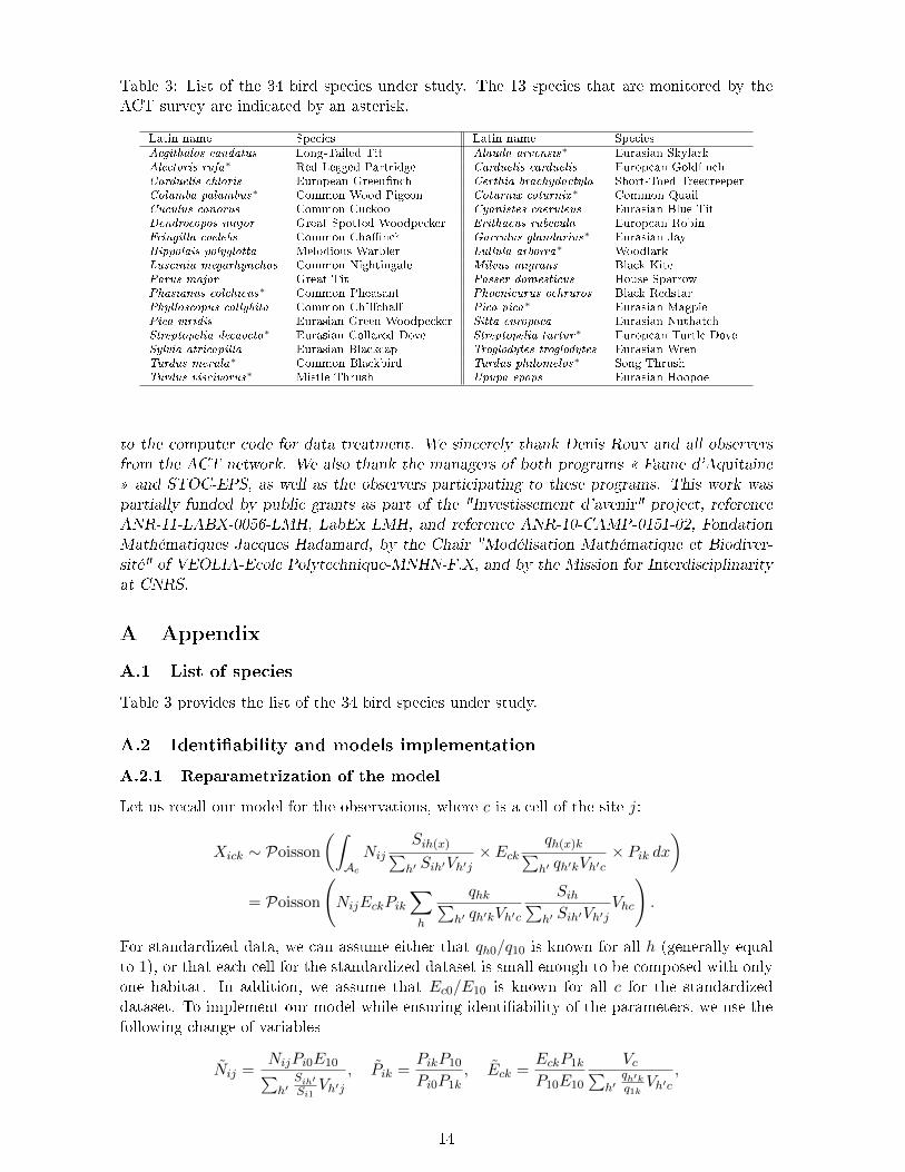
Table 3: List of the 34 bird species under study. The 13 species that are monitored by theACT survey are indicated by an asterisk.

Latin name Species Latin name Species

Aegithalos caudatus Long-Tailed Tit Alauda arvensis∗ Eurasian Skylark

Alectoris rufa∗ Red-Legged Partridge Carduelis carduelis European Gold�nch

Carduelis chloris European Green�nch Certhia brachydactyla Short-Toed Treecreeper

Columba palumbus∗ Common Wood Pigeon Coturnix coturnix∗ Common Quail

Cuculus canorus Common Cuckoo Cyanistes caeruleus Eurasian Blue Tit

Dendrocopos major Great Spotted Woodpecker Erithacus rubecula European Robin

Fringilla coelebs Common Cha�nch Garrulus glandarius∗ Eurasian Jay

Hippolais polyglotta Melodious Warbler Lullula arborea∗ Woodlark

Luscinia megarhynchos Common Nightingale Milvus migrans Black Kite

Parus major Great Tit Passer domesticus House Sparrow

Phasianus colchicus∗ Common Pheasant Phoenicurus ochruros Black Redstar

Phylloscopus collybita Common Chi�cha� Pica pica∗ Eurasian Magpie

Pica viridis Eurasian Green Woodpecker Sitta europaea Eurasian Nuthatch

Streptopelia decaocto∗ Eurasian Collared Dove Streptopelia turtur∗ European Turtle Dove

Sylvia atricapilla Eurasian Blackcap Troglodytes troglodytes Eurasian Wren

Turdus merula∗ Common Blackbird Turdus philomelos∗ Song Thrush

Turdus viscivorus∗ Mistle Thrush Upupa epops Eurasian Hoopoe

to the computer code for data treatment. We sincerely thank Denis Roux and all observers

from the ACT network. We also thank the managers of both programs � Faune d'Aquitaine

� and STOC-EPS, as well as the observers participating to these programs. This work was

partially funded by public grants as part of the "Investissement d'avenir" project, reference

ANR-11-LABX-0056-LMH, LabEx LMH, and reference ANR-10-CAMP-0151-02, Fondation

Mathématiques Jacques Hadamard, by the Chair "Modélisation Mathématique et Biodiver-

sité" of VEOLIA-Ecole Polytechnique-MNHN-F.X, and by the Mission for Interdisciplinarity

at CNRS.

A Appendix

A.1 List of species

Table 3 provides the list of the 34 bird species under study.

A.2 Identi�ability and models implementation

A.2.1 Reparametrization of the model

Let us recall our model for the observations, where c is a cell of the site j:

Xick ∼ Poisson

(∫Ac

Nij

Sih(x)∑h′ Sih′Vh′j

× Eck

qh(x)k∑h′ qh′kVh′c

× Pik dx

)= Poisson

(NijEckPik

∑h

qhk∑h′ qh′kVh′c

Sih∑h′ Sih′Vh′j

Vhc

).

For standardized data, we can assume either that qh0/q10 is known for all h (generally equalto 1), or that each cell for the standardized dataset is small enough to be composed with onlyone habitat. In addition, we assume that Ec0/E10 is known for all c for the standardizeddataset. To implement our model while ensuring identi�ability of the parameters, we use thefollowing change of variables

Nij =NijPi0E10∑h′

Sih′Si1

Vh′j, Pik =

PikP10

Pi0P1k, Eck =

EckP1k

P10E10

Vc∑h′

qh′kq1k

Vh′c,

14

qhk =qhkq1k

, Sih =SihSi1

where Vc =∑

h Vhc. Using this change of variables, we get that for all i, c and k,

Xick ∼ P

(NijEckPik

∑h

qhkSihVhc

)with

Nij

Ni1

=Nij

Ni1

∑h′ Sih′Vh′1∑h′ Sih′Vh′j

, Pi0 = 1, P11 = 1, ˜qh0 = 1, ˜q11 = 1, Si1 = 1

for all i, c, k, and Ec0 is known for all c.In particular for standardized data, for which we can assume that the habitat associated toeach cell c is known (denoted by h(c)), we get:

Xic0 ∼ P(NijEc0Sih(c)

),

where Ec0 is known for all cell c. This is a generalized linear model with IJ + I(H − 1)unknown parameters (the quantities Nij as well as habitat selection parameters Sih/Si1 forh > 1). These parameters are identi�able if and only if the matrix Y with size C×(J+H−1)giving for each cell c visited by the STOC dataset, the site and habitat associated to this cell(when this habitat is not the �rst habitat), has rank J +H − 1. More precisely, the matrix Yis such that for all c ∈ [[1, C]], Ycj(c) = 1, YcJ+(h(c)−1) = 1 if h(c) > 1, and Ycl = 0 elsewhere.

A.2.2 Implementation with JAGS

The computer code associated to the section 3.1 is given in the numerical Additional FileSimulatedData.Rnw. This program calls three models that are written in separate �les: onefor our model (Additional �le ModelSimulatedData.txt), one for the model in which we useonly standardized data (Additional �le ModelStandardizedSimulatedData.txt), and one forthe model in which di�erences in habitat preferences are neglected (Additional �le Model-WithoutHabitatSimulatedData.txt).The computer code associated to the section 2 is given in the numerical Additional File Real-Data.Rnw. This program calls four models that are written in separate �les: one for our model(Additional �le ModelWithHabitat.txt), one for the model in which we use only standardizeddata (Additional �le ModelStandardizedOnly.txt), one for the model in which di�erences inhabitat preferences are neglected (Additional �le ModelWithoutHabitat.txt), and one for themodel in space is considered as one single quadrat (Additional �le ModelOneQuadrat.txt).

A.3 Some details on the numerics: the prediction of the STOC data

Let CSTOCj denote the set of all the observation points c in the quadrat j surveyed in the

STOC dataset. The STOC counts for the species i in the quadrat j are

XSTOCij =

∑c∈CSTOC

j

XSTOCic .

15

Let us denote by h(c) the habitat type of the observation point c. In our model (2), theaverage number of individuals of the species i in the square c ∈ CSTOC

j is given by∫Ac

NijSih(c)∑h′ Sih′Vh′j

dx =NijSih(c)Vc∑

h′ Sih′Vh′j.

Taking into account a variable observational e�ort ESTOCc on each observation point c, we

then predict XSTOCij from the estimation based on our Model (2) by

Xmodelij = Nmodel

ij

∑c∈CSTOC

j

ESTOCc

Smodelih(c) Vc∑

h′ Smodelih′ Vh′j

,

where the observational e�ort ESTOCc is given by the number of years of observation at the

observation point c.For the one quadrat model with habitat [One Quadrat with hab] displayed in Table 2, theprediction is given by

Xmodelij = Nmodel

i

∑c∈CSTOC

j

ESTOCc

Smodelih(c) Vc∑

h′ Smodelih′ Vh′

,

with Vh′ the area of the habitat type h′ in the whole quadrat.When the Model (1) is used for estimation, then the predictions are given by

Xmodelij = Nij

∑c∈CSTOC

j

ESTOCc

VcVj.

A.4 Additional results on simulated data

In this section we provide additional results to the ones presented in Section 3.1 for simulateddata. Figure 5, as a complement to Figure 1, provides the posterior distributions of the habitatselection probabilities Si2 for all i, showing that these posterior are a good approximations tothe reference values that we wish to estimate. Figure ??, as a complement to Figure 1 givesthe boxplots of the mean of the squared di�erence between the posterior distribution and thereal value of relative abundances, for the di�erent considered models and datasets.

A.5 Additional results on real data

A.5.1 Some ecological results

In this section we provide additional results with ecological motivations.In Figure 6 we give a map of the estimated densities of the Grimpereau, with and withouthabitat struture. In Figure 7 we give the mean preferences of all considered species, for eachhabitat type.

16

Figure 5: Posterior distributions of the habitat selection probabilities Si2 for all i (Si1 = 1 forall i, each graph corresponds to a di�erent value of i). The reference values are given in red.

A.5.2 Taking into account habitat dependent detectability

We so far assumed that the detectability Pik of species i in dataset k does not depend onthe habitat, which might be unrealistic since, in particular, the range of vision (or hearing)can be di�erent from one habitat to the other. If so, our estimation of habitat selectionparameters Sih but also of species relative abundances can be biased. Due to identi�abilityconstraints, we cannot add and estimate an unknown list of parameters αh taking into accountthe dependence of detectability to habitat (since they will be undistinguishable from thespecies habitat selection probabilities Sih). Our proposition is to use an auxiliary dataset thatcan provide informations concerning the detectability associated to each considered habitat.We test this idea using a dataset provided by VigieNature that gives for di�erent kinds ofhabitats the respective numbers of observations made in di�erent ranges of distance. Theprogram associated to this section is given in the �le alpha.R.For each habitat h, we can assume that detection probability is equal to 1 when observedindividuals are "close enough" to the observer, since we only want to quantify the loss indetectability in each habitat due to the limitation in range of vision (or hearing) in thishabitat. More precisely, we assume that detection probability is equal to 1 when the observedindividual is less than 25 meters far from the observer. Then if we denote by Yh the number ofobserved individuals in habitat h and by Y1h the number of observed individuals in habitat h,at distance less than 25 meters from the observer, we can quantify the detectability in habitath by the quantity

αh =Yh/Y1hY1/Y11

.

The result of these calculations is given in Table 4. As expected, the detectability is lower

17

Figure 6: Relative density maps of the European nuthatch, without (left), and with (right)taking into account habitat structure. For each quadrat the gray level indicates the relative

densityNmodel

ij V1

Nmodeli1 Vj

where Vl is the area of quadrat l.

in urbanized area and forest than in open and agricultural landscapes. The impact of takinginto account habitat detectability is illustrated in Figure 7.

Corine land Cover Habitat Detectability αh

Urbanized area 1Intensive agriculture 1.72

Open natural landscape 1.71Farmland with heterogenous landscape 1.72

Mixed forest 1.47Deciduous forest 1.47Coniferous forest 1.47

Table 4: The detectability associated to each habitat, taking account di�erences in ranges ofvision.

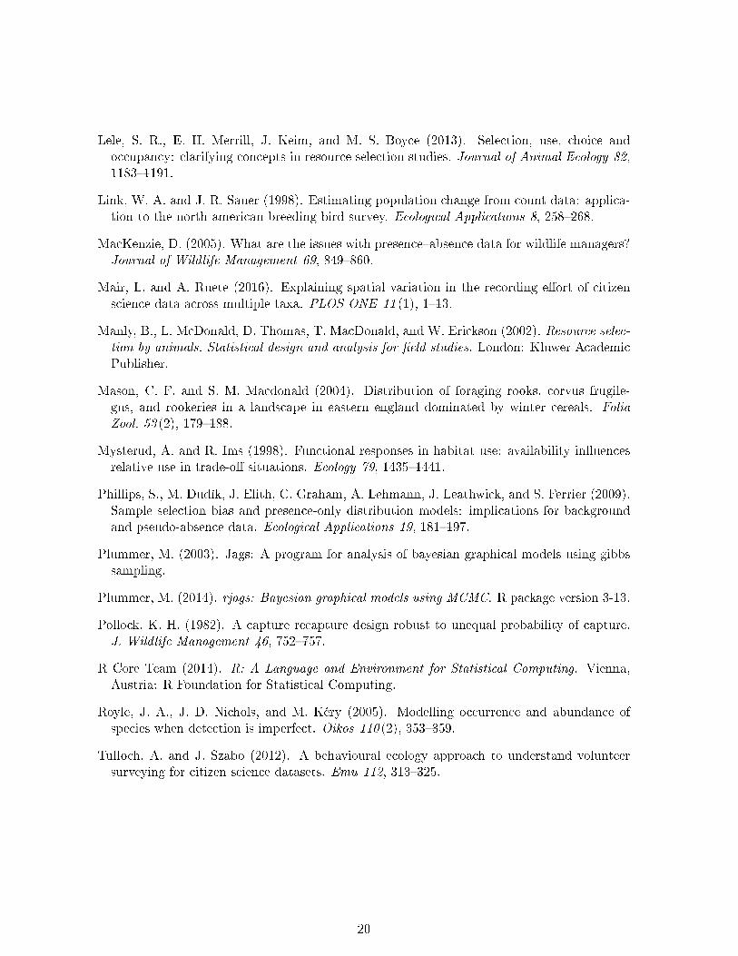
References

Bellamy, P. E., N. J. Brown, B. Enoksson, L. G. Firbank, R. J. Fuller, S. A. Hinsley, andA. G. M. Schotman (1998). The in�uences of habitat, landscape structure and climate onlocal distribution patterns of the nuthatch (sitta europaea l.). Oecologia 115 (1-2), 127�136.

18

Figure 7: Mean species estimated habitat selection probabilities, without (left) and with(right) habitat dependent detectability.

Biggs, C. R. and J. D. Olden (2011). Multi-scale habitat occupancy of invasive lion�sh (pteroisvolitans) in coral reef environments of roatan, honduras. Aquatic Invasions 6, 347�353.

Boutin, J., D. Roux, and C. Eraud (2003). Breeding bird monitoring in france: the act survey.Ornis Hungarica 12 (13), 1�2.

Boyce, M. and L. McDonald (1999). Relating populations to habitats using resource selectionfunctions. Trends in Ecology & Evolution 14, 268�272.

Buckland, S., D. Anderson, K. Burnham, and J. Laake (1993). Distance Sampling: EstimatingAbundance of Biological Populations. Chapman & Hall, New York.

Calenge, C., A. Dufour, and D. Maillard (2005). K-select analysis: a new method to analysehabitat selection in radio-tracking studies. Ecological Modelling 186, 143�153.

Dickinson, J. L., B. Zuckerberg, and D. N. Bonter (2010). Citizen science as an ecologicalresearch tool: Challenges and bene�ts. Annual Review of Ecology, Evolution, and System-

atics 41 (1), 149�172.

Fithian, W., J. Elith, T. Hastie, and D. Keith (2014). Bias correction in species distributionmodels: Pooling survey and collection data for multiple species. to appear in Methods for

Ecology and Evolution.

Fuller, R. M., B. J. Devereux, S. Gillings, G. S. Amable, and R. A. Hill (2005). Indices of bird-habitat preference from �eld surveys of birds and remote sensing of land cover: a study ofsouth-eastern england with wider implications for conservation and biodiversity assessment.Global Ecol. Biogeogr. 14, 223�239.

Giraud, C., C. Calenge, C. Coron, and R. Julliard (2015). Capitalizing on opportunistic datafor monitoring species relative abundances. Biometrics 72 (2), 649�58.

Isaac, N. J. B., A. J. van Strien, T. A. August, M. P. de Zeeuw, and D. B. Roy (2014). Statisticsfor citizen science: extracting signals of change from noisy ecological data. Methods in

Ecology and Evolution.

Jiguet, F., V. Devictor, R. Julliard, and D. Couvet (2012). French citizens monitoring ordinarybirds provide tools for conservation and ecological sciences. Acta Oecologica 44, 58 � 66.

19

Lele, S. R., E. H. Merrill, J. Keim, and M. S. Boyce (2013). Selection, use, choice andoccupancy: clarifying concepts in resource selection studies. Journal of Animal Ecology 82,1183�1191.

Link, W. A. and J. R. Sauer (1998). Estimating population change from count data: applica-tion to the north american breeding bird survey. Ecological Applications 8, 258�268.

MacKenzie, D. (2005). What are the issues with presence�absence data for wildlife managers?Journal of Wildlife Management 69, 849�860.

Mair, L. and A. Ruete (2016). Explaining spatial variation in the recording e�ort of citizenscience data across multiple taxa. PLOS ONE 11 (1), 1�13.

Manly, B., L. McDonald, D. Thomas, T. MacDonald, and W. Erickson (2002). Resource selec-tion by animals. Statistical design and analysis for �eld studies. London: Kluwer AcademicPublisher.

Mason, C. F. and S. M. Macdonald (2004). Distribution of foraging rooks, corvus frugile-gus, and rookeries in a landscape in eastern england dominated by winter cereals. Folia

Zool. 53 (2), 179�188.

Mysterud, A. and R. Ims (1998). Functional responses in habitat use: availability in�uencesrelative use in trade-o� situations. Ecology 79, 1435�1441.

Phillips, S., M. Dudík, J. Elith, C. Graham, A. Lehmann, J. Leathwick, and S. Ferrier (2009).Sample selection bias and presence-only distribution models: implications for backgroundand pseudo-absence data. Ecological Applications 19, 181�197.

Plummer, M. (2003). Jags: A program for analysis of bayesian graphical models using gibbssampling.

Plummer, M. (2014). rjags: Bayesian graphical models using MCMC. R package version 3-13.

Pollock, K. H. (1982). A capture recapture design robust to unequal probability of capture.J. Wildlife Management 46, 752�757.

R Core Team (2014). R: A Language and Environment for Statistical Computing. Vienna,Austria: R Foundation for Statistical Computing.

Royle, J. A., J. D. Nichols, and M. Kéry (2005). Modelling occurrence and abundance ofspecies when detection is imperfect. Oikos 110 (2), 353�359.

Tulloch, A. and J. Szabo (2012). A behavioural ecology approach to understand volunteersurveying for citizen science datasets. Emu 112, 313�325.

20