Estimation of Single Trial ERPs and EEG Phase ...epubs.surrey.ac.uk/804408/1/Jarchi2011.pdf ·...
144
University of Surrey Faculty of Engineering and Physical Sciences Department of Computing Computing Sciences Report PhD Thesis Estimation of Single Trial ERPs and EEG Phase Synchronization with Application to Mental Fatigue by Delaram Jarchi Supervisor: Dr Saeid Sanei Surrey, 2011 c 2011 Delaram Jarchi
Transcript of Estimation of Single Trial ERPs and EEG Phase ...epubs.surrey.ac.uk/804408/1/Jarchi2011.pdf ·...

University of Surrey
Faculty of Engineering and Physical Sciences
Department of Computing
Computing Sciences Report
PhD Thesis
Estimation of Single Trial ERPs and
EEG Phase Synchronization
with Application to Mental Fatigue
by
Delaram Jarchi
Supervisor: Dr Saeid Sanei
Surrey, 2011
c©2011 Delaram Jarchi

To my parents who grew me up without any expectation

Abstract
Monitoring mental fatigue is a crucial and important step for prevention of fatal
accidents. This may be achieved by understanding and analysis of brain electrical
potentials. Electroencephalography (EEG) is the record of electrical activity of
the brain and gives the possibility of studying brain functionality with a high
temporal resolution. EEG has been used as an important tool by researchers for
detection of fatigue state. However, their proposed methods have been limited
to classical statistical solutions and the results given by different researchers are
somehow conflicting. Therefore, there is a need for modification of the existing
methods for reliable analysis of mental fatigue and detection of fatigue state.
In addition to the raw EEG, event related potentials (ERPs), which are direct
measures of brain responses to the specified stimuli, have been used in mental
fatigue analysis since the attention related ERPs have shown to be effective for
detection of fatigue state. In this study we aim to extend and further develop
the existing signal processing methods for EEG- and ERP-based mental fatigue
analysis.
First, a new approach is proposed for measuring synchronization of EEG os-
cillations in different frequency bands across brain regions. The approach is used
to find the relevant and effective features for detection of the fatigue state. It uses
adaptive methods such as empirical mode decomposition (EMD) and adaptive
line enhancer (ALE) for extracting and de-noising the EEG oscillations. Then,
Hilbert transform (HT) is used for computing the linear and non-linear synchro-
nization measures. A new method based on particle filtering (PF) is proposed
for direct estimation of instantaneous phase of an oscillation. This method can
be developed more in future studies for phase synchronization analysis of the
EEG oscillations before and during the fatigue state.
ERP subcomponents are estimated using PF. Based on the proposed method,
ERP subcomponents are separated in temporal domain across different trials and
their inter-trial variability is tracked using a coupled PF. The method is applied
to mental fatigue data to show the potential use of the method in ERP subcom-
ponent estimation for detection of fatigue state. Then, a new spatio-temporal
i

filtering is designed for estimation of the correlated ERP subcomponents. The
method is robust against both temporal and spatial correlations of the ERP sub-
components. It is compared to the existing methods in different scenarios and
its superiority is confirmed by using simulated signals. It is also applied to real
data to show its potential use in ERP subcomponent estimation.
Finally, an auditory based paradigm is implemented to evaluate the effective-
ness of the designed mental fatigue detection system. By applying the proposed
methods for estimation of single trial P300 subcomponents and EEG phase syn-
chronization, it is demonstrated that the proposed auditory paradigm can be
effectively used in a mental fatigue detection system.

Acknowledgements
I would like to thank Dr. Sanei, my supervisor, for his many valuable sugges-
tions and continuous support during this research. His enthusiastic supervision,
invaluable input, great encouragement have provided a wonderful basis for the
present study. I very much appreciate his support from the beginning in all the
aspects.
I am thankful to Prof. Principe at University of Florida and Dr. Lorist
at Groningen University, Netherland for their valuable comments about ERP
detection and mental fatigue analysis respectively. I am also thankful to Mr
Dean at the Department of Psychology, University of Surrey, for his help in
EEG recording. I am also thankful to the Leverhulme Trust for its financial
support.
Guildford, Surrey Delaram Jarchi
June 2011
iii
Table of Contents
Abstract i
Acknowledgements iii
Table of Contents iv
List of Publications vii
List of Tables ix
List of Figures ix
List of Abbreviations xv
Nomenclatures xvii
1 Introduction 1
1.1 Aim and Objectives . . . . . . . . . . . . . . . . . . . . . . . . . 2
1.2 Thesis Outline . . . . . . . . . . . . . . . . . . . . . . . . . . . . 2
2 Overview of EEG and ERP 4
2.1 Electroencephalography . . . . . . . . . . . . . . . . . . . . . . . 4
2.1.1 EEG Recording . . . . . . . . . . . . . . . . . . . . . . . . 4
2.1.2 EEG versus fMRI, PET and MEG . . . . . . . . . . . . . 6
2.1.3 EEG Rhythmic Activities . . . . . . . . . . . . . . . . . . 7
2.2 Event Related Potentials . . . . . . . . . . . . . . . . . . . . . . . 8
2.2.1 P300 . . . . . . . . . . . . . . . . . . . . . . . . . . . . . . 9
2.3 Summary . . . . . . . . . . . . . . . . . . . . . . . . . . . . . . . 10
3 Recognition of Mental Fatigue: Tools and Algorithms 11
3.1 Fatigue and its Research Motivation . . . . . . . . . . . . . . . . 11
3.2 EEG-based Analysis of Mental Fatigue . . . . . . . . . . . . . . . 12
3.3 ERP-based Analysis of Mental Fatigue . . . . . . . . . . . . . . . 14
3.4 Fundamentals of KF, Basic PF, and RBPF . . . . . . . . . . . . 16
3.4.1 Problem Formulation in State Space . . . . . . . . . . . . 17
3.4.2 Kalman Filtering . . . . . . . . . . . . . . . . . . . . . . . 18
iv

3.4.3 Particle Filtering . . . . . . . . . . . . . . . . . . . . . . . 19
3.4.4 Rao-Blackwellised Particle Filtering . . . . . . . . . . . . 20
3.5 Summary . . . . . . . . . . . . . . . . . . . . . . . . . . . . . . . 22
4 Estimation of EEG Phase Synchronization with Application to
Mental Fatigue 23
4.1 Introduction . . . . . . . . . . . . . . . . . . . . . . . . . . . . . . 23
4.2 Empirical Mode Decomposition . . . . . . . . . . . . . . . . . . . 24
4.3 Adaptive Line Enhancer . . . . . . . . . . . . . . . . . . . . . . . 25
4.4 Synchronization Measures . . . . . . . . . . . . . . . . . . . . . . 27
4.4.1 Linear Measure of Synchronization . . . . . . . . . . . . . 27
4.4.2 Non-linear Measure of Synchronization . . . . . . . . . . . 28
4.5 Experimental Results . . . . . . . . . . . . . . . . . . . . . . . . . 28
4.5.1 Simulated Data . . . . . . . . . . . . . . . . . . . . . . . . 28
4.5.2 Real Data . . . . . . . . . . . . . . . . . . . . . . . . . . . 30
4.6 Instantaneous Phase Tracking of EEG Oscillations using EMD
and RBPF . . . . . . . . . . . . . . . . . . . . . . . . . . . . . . . 38
4.6.1 Problem Formulation using RBPF . . . . . . . . . . . . . 39
4.6.2 Application . . . . . . . . . . . . . . . . . . . . . . . . . . 44
4.6.2.1 Simulated Results . . . . . . . . . . . . . . . . . 44
4.6.2.2 Real Data Results . . . . . . . . . . . . . . . . . 45
4.7 Conclusions . . . . . . . . . . . . . . . . . . . . . . . . . . . . . . 46
5 Coupled RBPF for Single Trial Estimation of ERPs in Temporal
Domain with Application to Mental Fatigue 48
5.1 Introduction . . . . . . . . . . . . . . . . . . . . . . . . . . . . . . 48
5.2 Problem Formulation using PF . . . . . . . . . . . . . . . . . . . 50
5.3 Coupled RBPF Formulation . . . . . . . . . . . . . . . . . . . . . 51
5.4 Experimental Results . . . . . . . . . . . . . . . . . . . . . . . . . 56
5.4.1 Simulated Data . . . . . . . . . . . . . . . . . . . . . . . . 56
5.4.2 Real Data . . . . . . . . . . . . . . . . . . . . . . . . . . . 62
5.5 Conclusions . . . . . . . . . . . . . . . . . . . . . . . . . . . . . . 65
6 Spatio-temporal Filtering Method for Single Trial Estimation of
Correlated ERP Subcomponents 67
6.1 Introduction . . . . . . . . . . . . . . . . . . . . . . . . . . . . . . 67
6.2 Linear Generative EEG Model . . . . . . . . . . . . . . . . . . . 69
6.3 Spatio-temporal Filtering Method . . . . . . . . . . . . . . . . . . 71
6.4 Simulation Results . . . . . . . . . . . . . . . . . . . . . . . . . . 78
6.4.1 PCA, Temporal PCA, Spatial PCA, and Spatio-temporal
PCA . . . . . . . . . . . . . . . . . . . . . . . . . . . . . . 79
6.4.2 Comparison Study . . . . . . . . . . . . . . . . . . . . . . 85
6.5 Real Data Results . . . . . . . . . . . . . . . . . . . . . . . . . . 91
6.6 Conclusions . . . . . . . . . . . . . . . . . . . . . . . . . . . . . . 98

7 Implementation of EEG-based and ERP-based Approaches to
Detection of Mental Fatigue; an Auditory Based Paradigm 100
7.1 Introduction . . . . . . . . . . . . . . . . . . . . . . . . . . . . . . 100
7.2 Experimental Setup . . . . . . . . . . . . . . . . . . . . . . . . . 101
7.3 Estimation of Single Trial P300 Subcomponents . . . . . . . . . . 101
7.4 Estimation of EEG Phase Synchronization . . . . . . . . . . . . . 106
7.5 Conclusions . . . . . . . . . . . . . . . . . . . . . . . . . . . . . . 106
8 Summary, Conclusions and Future Works 109
8.1 Summary and Conclusions . . . . . . . . . . . . . . . . . . . . . . 109
8.2 Future Works . . . . . . . . . . . . . . . . . . . . . . . . . . . . . 111
Bibliography 112

List of Publications
Journal
[1] D. Jarchi, S. Sanei, J. C. Principe and B. Makkiabadi, “A new spatiotem-
poral filtering method for single-trial estimation of correlated ERP subcom-
ponents”, IEEE Transactions on Biomedical Engineering, Volume 58, Issue
1, January 2011.
[2] D. Jarchi, S. Sanei, H. R. Mohseni, and M. M. Lorist, “Coupled particle
filtering: A new approach for P300-based analysis of mental fatigue”, Journal
of Biomedical Signal Processing and Control, Volume 6, Issue 2, April 2011.
Conference
[1] D. Jarchi, B. Makkiabadi, and S. Sanei, “Instantaneous phase tracking of
oscillatory signals using EMD and Rao-blackwellised particle filtering”, In
proc. IEEE International Conf. on Acoustic, Speech and Signal Processing,
ICASSP 2011, Prague, Czech Republic.
[2] D. Jarchi, B. Makkiabadi, and S. Sanei, “A new spatiotemporal filtering
method for single trial ERP subcomponent estimation”, In proc. European
Signal Processing Conference, EUSIPCO 2010, Aalborg, Denmark.
[3] D. Jarchi, B. Makkiabadi, and S. Sanei, “Mental fatigue analysis by measur-
ing synchronization of brain rhythms incorporating empirical mode decom-
position”, In proc. 2nd International Workshop on Cognitive Information
Processing, CIP 2010, Elba, Italy.
[4] D. Jarchi, B. Makkiabadi, and S. Sanei, “Estimation of trial to trial variabil-
ity of P300 subcomponents by coupled Rao-blackwellised particle filtering”,
In proc. IEEE Workshop on Statistical Signal Processing, SSP 2009, Cardiff,
UK.
vii
[5] D. Jarchi, and S. Sanei, “Source Localization of Brain Rhythms by Empir-
ical Mode Decomposition and Spatial Notch Filtering” In proc. European
Signal Processing Conference, EUSIPCO 2009, Glasgow, Scotland.
[6] D. Jarchi, B. Makkiabadi, and S. Sanei, “Separating and tracking ERP
subcomponents using constrained particle filter,” In proc. 16th Int. Conf.
on Digital Signal Processing, DSP 2009, Santorini, Greece.
Contribution as Co-author
Journal
[1] J. Escudero, S. Sanei, D. Jarchi, D. Abasolo and R. Hornero, “Regional
coherence evaluation in mild cognitive impairment and Alzheimer’s disease
based on adaptively extracted magnetoencephalogram rhythms”, Physiolog-
ical measurement, Volume 32, Issue 8, August 2011.
Conference
[1] B. Makkiabadi, D. Jarchi and S. Sanei, “Simultaneous localization and
separation of biomedical signals by tensor factorization”, In proc. IEEE
Workshop on Statistical Signal Processing, SSP 2009, Cardiff, UK.
[2] B. Makkiabadi, A. Sarrafzadeh, D. Jarchi, V. Abolghasemi and S. Sanei,
“Semi-blind signal separation and channel estimation in MIMO communica-
tion systems by tensor factorization”, In proc. IEEE Workshop on Statistical
Signal Processing, SSP 2009, Cardiff, UK.
[3] V. Abolghasemi, D. Jarchi, and S. Sanei, “A robust approach for optimiza-
tion of measurement matrix in compressive sensing”, In proc. 2nd Inter-
national Workshop on Cognitive Information Processing, CIP 2010, Elba,
Italy.
[4] B. Makkiabadi, D. Jarchi, V. Abolghasemi, and S. Sanei, “A Time Do-
main Geometrically Constrained Multimodal Approach for Convolutive Blind
Source Separation”, In proc. EUSIPCO 2011, Barcelona, Spain.
[5] B. Makkiabadi, D. Jarchi and S. Sanei, “Blind Separation and Localiza-
tion of Correlated P300 Subcomponents Subcomponents from Single Trial
Recordings using Tensor Model”, In proc. EMBC 2011, Boston , MA, USA.

List of Tables
4.1 MSE of the phase in two SNR levels. . . . . . . . . . . . . . . . . 44
6.1 Scalp projection estimation for P300 subcomponents in different
SNRs for different methods. The values are mean correlation co-
efficients between the estimated and actual scalp projections in
40 trials . . . . . . . . . . . . . . . . . . . . . . . . . . . . . . . . 87
6.2 Amplitude estimation for P300 subcomponents in different SNRs
for different methods. The values are means and variances of the
ratios between the actual and estimated amplitudes in 40 trials. . 88
6.3 Latency estimation for P300 subcomponents in different SNRs
for different methods. The values are means and variances of the
estimated latencies in 40 trials. . . . . . . . . . . . . . . . . . . . 89
6.4 P300 subcomponents parameter estimation at SNR = 0 dB con-
sidering background EEG as noise. . . . . . . . . . . . . . . . . . 90
6.5 Effects of Mismatch in P300 subcomponents descriptor’s estimation. 91
ix

List of Figures
2.1 75-pin electrode positions based on extended 10-20 system [http://www-
psych.nmsu.edu/ jkroger/lab/principles.html]. . . . . . . . . . . . 5
4.1 Block diagram of an adaptive line enhancer system for denoising
and enhancing an IMF. . . . . . . . . . . . . . . . . . . . . . . . 26
4.2 (a) The noisy mixture signal (first), actual EEG oscillation in
beta frequency band (second), the extracted IMF (third), and the
line enhanced IMF (fourth). (b) The resulted HS of the actual
source (top), extracted IMF (middle) and the line enhanced IMF
(bottom). The colour bar represents the instantaneous amplitude. 29
4.3 Interhemisphere coherence of beta, alpha and theta rhythms, the
top row corresponds to the fatigue state and the bottom row cor-
responds to the alert state. . . . . . . . . . . . . . . . . . . . . . 32
4.4 Interhemisphere phase synchronization of beta (left), alpha (mid-
dle), and theta (right) rhythms. . . . . . . . . . . . . . . . . . . 33
4.5 Phase synchronization of beta (top), alpha (middle), and theta
(bottom) rhythms around stimulus onset. . . . . . . . . . . . . . 34
4.6 Coherence of alpha rhythm around stimulus onset for before fa-
tigue (top row) and during fatigue (bottom row). Dark blue colour
presents lack of coherence and dark red colour presents the max-
imum coherence. . . . . . . . . . . . . . . . . . . . . . . . . . . . 35
4.7 Coherence of beta rhythm around stimulus onset for before fatigue
(top row) and during fatigue (bottom row). Dark blue colour
presents lack of coherence and dark red colour presents the max-
imum coherence. . . . . . . . . . . . . . . . . . . . . . . . . . . . 36
4.8 Coherence of theta rhythm around stimulus onset for before fa-
tigue (top row) and during fatigue (bottom row). Dark blue colour
presents lack of coherence and dark red colour presents the max-
imum coherence. . . . . . . . . . . . . . . . . . . . . . . . . . . . 37
x

4.9 IP (top two rows) and IA (bottom two rows) estimation using the
proposed and HT methods in two SNR levels. . . . . . . . . . . . 45
4.10 IF estimation using the proposed (dotted line) and HT (bold red
line) methods in two SNR levels of 7.2dB (top) and 3dB (bottom). 46
4.11 IP (tow row) and IA (bottom row) estimation of C3 channel using
the proposed method. . . . . . . . . . . . . . . . . . . . . . . . . 47
4.12 IF estimation of C3 channel using the proposed method. . . . . . 47
5.1 The latency, amplitude, and width of the simulated P3a and P3b
at Fz are used as the states of RBPF1 and at Pz as the states of
RBPF2. Each particle pair has the same width value for P3a at
Fz and Pz channels, and has the same width value for P3b at Fz
and Pz channels. . . . . . . . . . . . . . . . . . . . . . . . . . . . 54
5.2 Tracking the latency, amplitude, and width of simulated P3a and
P3b on channels Fz (a,b,e,f) and Pz (c,d,g,h) using CRBPF; the
thick line connects the actual values while the dotted line is the
result of estimation and tracking using CRBPF. . . . . . . . . . 57
5.3 The corresponding MSE, (a) and (c), and SNR, (b) and (d), cal-
culated in different trials for the simulated data for Fz (top) and
Pz (bottom) channels. . . . . . . . . . . . . . . . . . . . . . . . . 59
5.4 Two Gamma waves are used for modelling P3a and P3b. Different
Gaussians approximating Gamma waves are also shown. . . . . . 60
5.5 The dotted lines are the results of tracking using CRBPF, (a)
latency variations of P3a (red line) and P3b (Blue line) on channel
Fz, (b) amplitude variations of P3a (red line) and P3b (Blue line)
on channel Fz, (c) MSE obtained at each trial for channel Fz, (d)
calculated SNR at each trial for channel Fz, (e) latency variations
of P3a (red line) and P3b (Blue line) on channel Pz, (f) amplitude
variations of P3a (red line) and P3b (Blue line) on channel Pz,
(g) MSE obtained at each trial for channel Pz, and (h) calculated
SNR at each trial for channel Pz. . . . . . . . . . . . . . . . . . 61

5.6 The dotted lines are the results of tracking using CRBPF, (a)
latency variations of P3a (red line) and P3b (Blue line) on channel
Fz, (b) amplitude variations of P3a (red line) and P3b (Blue line)
on channel Fz, (c) MSE obtained at each trial for channel Fz, (d)
calculated SNR at each trial for channel Fz, (e) latency variations
of P3a (red line) and P3b (Blue line) on channel Pz, (f) amplitude
variations of P3a (red line) and P3b (Blue line) on channel Pz,
(g) MSE obtained at each trial for channel Pz, and (h) calculated
SNR at each trial for channel Pz. . . . . . . . . . . . . . . . . . 63
5.7 Tracking variability of P3a and P3b before and during fatigue;
the left column corresponds to the before fatigue state (a,c,e,g,i,k)
while the right column to the during fatigue state (b,d,f,h,j,l). . . 64
6.1 Synthetic and presumed reference signals for P3a and P3b used
in the simulation study. The waveforms with dotted lines repre-
sent different approximations for actual signals and two of them
are selected as the presumed reference signals for simulating the
Mismatch case. . . . . . . . . . . . . . . . . . . . . . . . . . . . . 85
6.2 Locations of the simulated P3a and P3b inside the brain; (a)
transverse view, (b) sagittal view. . . . . . . . . . . . . . . . . . . 86
6.3 Comparison between three methods (spatial PCA, Exact Match
and Mismatch) with respect to the correlation coefficient between
the original and estimated scalp projections of P3a (left column)
and P3b (right column) in different spatial correlations and two
SNR levels of -5 dB (top row) and 0 dB (bottom row). . . . . . . 92
6.4 Comparison between three methods (temporal PCA, Exact Match
and Mismatch) with respect to the correlation coefficient between
the original and estimated scalp projections of P3a (left column)
and P3b (right column) in different temporal correlations and two
SNR levels of -5 dB (top row) and 0 dB (bottom row). . . . . . . 93
6.5 In the top row, the correlation coefficient between the original and
estimated scalp projections of P3a and P3b obtained by the three
methods (spatial PCA, Exact Match and Mismatch) in each trial
are shown. In the bottom row, single trial estimation of latencies
of P3a and P3b obtained by the three methods (spatial PCA,
Exact Match and Mismatch) in each trial are shown. . . . . . . . 94

6.6 In the top row, single trial estimation of amplitudes of P3a and
P3b obtained by the three methods (spatial PCA, Exact Match
and Mismatch) in each trial are shown. In the bottom row, SNR
and temporal correlations between P3a and P3b in each trial are
shown. . . . . . . . . . . . . . . . . . . . . . . . . . . . . . . . . . 95
6.7 Single Trial ERPs (40 trials related to the infrequent tones) and
their average from channel Fz. . . . . . . . . . . . . . . . . . . . 96
6.8 Selection of reference signals for P3a and P3b. In each row, the
reference signals for P3a and P3b with their estimated scalp pro-
jections are shown. By sliding the reference signals towards and
away from the averaged P300 and varying their shapes, the ob-
served changes in their estimated scalp projections are helpful for
reference selection. The reference signals shown in the middle row
which have high correlation with the averaged P300 are used as
good candidates for approximating the actual P3a and P3b. . . . 96
6.9 estimated amplitudes for P3a and P3b in different trials. . . . . . 97
6.10 Scalp projections of P3a in four selected progressive trials. . . . . 98
6.11 Scalp projections of P3b in four selected progressive trials. . . . . 98
7.1 The electrode names (left) and numbers (right) which used in the
experiment. . . . . . . . . . . . . . . . . . . . . . . . . . . . . . 102
7.2 This GUI generates two random integers any time the subject
presses ENTER key on the keyboard or ‘Submit’ button. . . . . 102
7.3 Forty single trial ERPs and their average from Cz channel before
fatigue. . . . . . . . . . . . . . . . . . . . . . . . . . . . . . . . . 104
7.4 Forty single trial ERPs and their average from Cz channel during
fatigue state. . . . . . . . . . . . . . . . . . . . . . . . . . . . . . 104
7.5 The averaged ERP of forty trials before and during fatigue state
from Cz channel. . . . . . . . . . . . . . . . . . . . . . . . . . . 104
7.6 The estimated P3a amplitudes in single trials before and during
fatigue state. . . . . . . . . . . . . . . . . . . . . . . . . . . . . . 105
7.7 The estimated P3b amplitudes in single trials before and during
fatigue state. . . . . . . . . . . . . . . . . . . . . . . . . . . . . . 105
7.8 The estimated scalp projections of P3a (top row) and P3b (bottom
row) before fatigue. . . . . . . . . . . . . . . . . . . . . . . . . . 105
7.9 The estimated scalp projections of P3a (top row) and P3b (bottom
row) during fatigue. . . . . . . . . . . . . . . . . . . . . . . . . . 106
7.10 Theta phase synchronization of F3-F4; (a) before stimulus and
(b) after stimulus . . . . . . . . . . . . . . . . . . . . . . . . . . . 107

7.11 Alpha phase synchronization of C3-C4; (a) before stimulus and
(b) after stimulus . . . . . . . . . . . . . . . . . . . . . . . . . . . 107
7.12 Beta phase synchronization of F3-F4; (a) before stimulus and (b)
after stimulus . . . . . . . . . . . . . . . . . . . . . . . . . . . . . 107

List of Abbreviations
ALE Adaptive Line Enhancer
ApEn Approximate Entropy
BCI Brain-Computer Interface
BSS Blind Source Separation
CRBPF Coupled RBPF
ECoG Electrocorticography
EEG Electroencephalography
EMD Empirical Mode Decomposition
EOG Electro-oculogram
ERP Event Related Potential
ERS Event Related Synchronization
fMRI Functional Magnetic Resonance Imaging
HMM Hidden Markov Model
HS Hilbert Spectrum
HT Hilbert Transform
IA Instantaneous Amplitude
ICA Independent Component Analysis
IF Instantaneous Frequency
IMF Intrinsic Mode Function
IP Instantaneous Phase
Kc Kolmogorov Complexity
KF Kalman Filtering
KPCA Kernel Principal Component Analysis
xv

LMS Least Mean Square
MAP Maximum A Posteriori
MEG Magnetoencephalography
MSE Mean Square Error
PCA Principal Component Analysis
PET Positron Emission Tomography
PF Particle Filtering
RBPF Rao-Blackwellized Particle Filtering
RF Random Forests
SNR Signal to Noise Ratio
SQUID Super Conducting Interference Device
SVD Singular Value Decomposition
WGN White Gaussian Noise
Nomenclatures
ai(t) Instantaneous amplitude of ith IMF at time t
at(i) Instantaneous amplitude of ith IMF at time t
ak(i) Amplitude of ith subcomponent at trial k
aik Amplitude of P3a in kth trial of ith RBPF
a(n)t Instantaneous amplitude of nth particle at time (trial) t
a(n)i
k nth particle for amplitude of P3a in kth trial of ith RBPF
aik Linear state of ith RBPF at trial k
a1 Scalp projection of ERP subcomponent
a2 Scalp projection of ERP subcomponent
aik Amplitude of P3b in kth trial of ith RBPF
a(n)i
k nth particle for amplitude of P3b in kth trial of ith RBPF
bk(i) Latency of ith subcomponent at trial k
bik Latency of P3a in kth trial of ith RBPF
b(n)i
k nth particle for latency of P3a in kth trial of ith RBPF
bk kth principal component
B Number of frequency bins
Bk−1(x1k−1) State transition for linear state variable of RBPF
bik Latency of P3b in kth trial of ith RBPF
b(n)i
k nth particle for latency of P3b in kth trial of ith RBPF
c Normalizing constant for Gamma waveform
ci(t) Analytic version of ith IMF at time t
Ck(x1k) Observation transition for linear state variable of RBPF
di(t) ith IMF at time t
dt(i) ith IMF at time t
diff(.) Differences between adjacent elements
e(t) Adaptation error of ALE at time t
xvii
exp(.) Exponential function
E. Expected value
f Observation transition function of PF
f State transition function of RBPF
fk General non-linear function
freq(n)t Instantaneous frequency of nth particle at time (trial) t
Fk State transition matrix in KF
f State transition function of RBPF
G Observation transition function of RBPF
G Observation transition function of RBPF
G′ Non-linear function
hk General non-linear function
hi(k, t) Hilbert transform of ith IMF at time t and kth frequency bin
Hk Observation transition matrix in KF
Hd[.] Discrete Hilbert transform
J√−1
k Shape parameter for Gamma waveform
kmax Number of trials
Kk Kalman gain
log(.) Logarithm function
M Number of IMFs
Ns Number of particles
nk−1 State noise of KF and PF
N (m,P) Gaussian distribution with mean m and covariance matrix P
N (x;m,P) Gaussian distribution with mean m and covariance matrix P evaluated at x
p Number of ERP subcomponents
Pk Covariance matrix of linear state vector variable of RBPF at trial k
p(.) Probability density function
p(.|.) Conditional probability density function
Psignal Power of signal
Pnoise Power of noise
q(.) Importance density function

Qw(ρi)k−1 Covariance matrix of state noise of non-linear state variable of ith RBPF
Qw(ai)k−1 Covariance matrix of state noise of linear state variable of ith RBPF
Qwt−1 Covariance matrix of state noise of RBPF
Qvt Covariance matrix of measurement noise of RBPF
Qnk−1 Covariance matrix of the state noise of KF
Qvk Covariance matrix of the measurement noise of KF and RBPF
Qwk−1 Covariance matrix of state noise for linear state variable of RBPF
r1 Temporal reference signal for ERP subcomponent
r2 Temporal reference signal for ERP subcomponent
Real(.) Real part of a complex variable
sik Width of P3a in kth trial of ith RBPF
s(n)i
k nth particle for width of P3a in kth trial of ith RBPF
sk(i) Width of ith subcomponent at trial k
sik Width of P3b in kth trial of ith RBPF
s(n)i
k nth particle for width of P3b in kth trial of ith RBPF
tmax Number of time points (trials)
Ts Sampling period
u(t− ∆) input vector of ALE at time t
unwrap(.) Phase unwrapping
vk Measurement noise of KF, PF and RBPF
vt Measurement noise of RBPF
Var Variance
w(t) Coefficient vector of ALE at time t
w(n)i
k Weight of nth particle of ith RBPF at trial k
w(n)t Weight of nth particle of RBPF at at time (trial) t
w(i)k Weight of ith particle at trial k
wρik−1 State noise of non-linear state variable of ith RBPF
wak−1 State noise of linear state variable of ith RBPF
w2k−1 State noise for linear state variable of RBPF
wt−1 State noise of RBPF
x(t) Signal (time series) value at time t
x1k Non-linear state of RBPF at trial k
x2k Linear state of RBPF at trial k
xk State of KF, PF and RBPF at trial k

xik ith particle at trial k
X Mixture matrix
zk Measurment at trial k
(.)T Transpose operation
δ(.) Dirac delta function
µ Step size in ALE
‖.‖2 Frobenious norm
θi(t) Instantaneous phase of ith IMF at time t
θt(i) Instantaneous phase of ith IMF at time t
χi,j(k) Cross spectrum of the ith and jth IMFs at kth frequency bin
ψi(k) Marginal power spectra of ith IMF at kth frequency bin
ζij(k) Coherence of ith and jth IMFs at kth frequency bin
γij Phase synchronization of ith and jth IMFs∂(.)∂wT Gradient with respect to wT
θ(n)t Instantaneous phase of nth particle at time (trial) t
ρ1t (i) Non-linear state of RBPF for ith IMF at time (trial) t
ρ2t (i) Linear state of RBPF for ith IMF at time (trial) t
µk Mean of linear state vector variable of RBPF at trial k
ρt State of RBPF at time (trial) t
ρ1t Non-linear state of RBPF at time (trial) t
ρ2t Linear state of RBPF at time (trial) t
ρt(i) State of RBPF for ith IMF at time (trial) t
ρik Non-linear state of ith RBPF at trial k
ρ(n)i
k nth particle of ith RBPF at trial k
θ Scale parameter for Gamma waveform
θestimate(t) Estimated phase at time t
θactual(t) Actual phase at time t
∆ Prediction depth of ALE
π Ratio of any circle’s circumference to its diameter (3.14159)
ωi(t) Instantaneous frequency of ith IMF at time t
Chapter 1
Introduction
Mental Fatigue refers to a state of the brain that is accompanied by reduced
mental performance. It has been a major cause for many accidents especially
in transportation (among drivers) and the aviation area such as military avia-
tion. Therefore, detection of fatigue state of a human operator is necessary for
prevention of disastrous accidents. Invention of electroencephalography (EEG)
for recording brain electrical activity has made it possible to have a deep and
comprehensive understanding of brain functionality. EEG is used as a technique
for analysing physiological based changes of the brain in the fatigue state [1].
However, evaluating EEG signal for mental fatigue analysis has been limited to
the classical signal processing methods. The development of signal processing
methods for a better detection of fatigue state from EEG signals is therefore
necessary. One research direction in this thesis is to extend and further develop
the existing signal processing methods for mental fatigue analysis using the EEG
signal.
There is a subgroup of electric signals from the brain using the EEG sys-
tems called event related potentials (ERPs). ERPs are responses of the brain to
specifically designed stimuli. Extracting and evaluating the ERPs lead to under-
standing of various brain functions. For mental fatigue analysis, different ERP
components and subcomponents are evaluated before and during the fatigue
state. It is reported that attention related ERPs can be helpful for identification
of the fatigue state [1]. Traditionally, ERPs are averaged over a number of trials
because of their low signal to noise ratio (SNR). However averaging ERPs over
a number of trials leads to the loss of information related to inter-trial variabil-
ity of ERPs. Inter-trial variability of ERPs can provide useful information for
detecting the fatigue state. Also, in the case of having correlated ERP subcom-
ponents in temporal or spatial domain the classical methods such as principal
component analysis (PCA), which is used for separation of correlated ERP sub-
components, fail. Therefore, another direction in this thesis is provision of new
1

1.1. AIM AND OBJECTIVES 2
methods for effective extraction of ERPs which exploit the inter-trial variability
of ERPs and overcome the problem of temporal/spatial correlation between the
ERP subcomponents. Then, the estimated ERPs can be used for detection of
fatigue state.
1.1 Aim and Objectives
In this thesis we aim to develop signal processing methods which are helpful for
better estimation of ERPs and EEG phase synchronization. The new insights
provided by the proposed methods for estimation of ERPs and EEG phase syn-
chronization are new effective basis for mental fatigue analysis and detecting the
fatigue state. Therefore, the main objective of this thesis has been on proposing
new methods to be used for reliable detection of the fatigue state. This thesis
represents significant contribution in the following areas:
• Estimation of EEG phase synchronization using combination of empiri-
cal mode decomposition (EMD) and adaptive line enhancer (ALE) with
application to mental fatigue for extracting the relevant features.
• Proposing a new method for phase tracking of the oscillatory signals based
on particle filtering (PF).
• Separation and tracking of P300 subcomponents overlapped in temporal
domain using a new formulation of PF.
• Proposing a new spatio-temporal filtering method for estimation of corre-
lated ERP subcomponents.
1.2 Thesis Outline
The layout of the thesis is as follows. In Chapter 2, the EEG recording procedure
is briefly described. Then, the EEG advantages and disadvantages in comparison
with other data acquisition modalities for recording brain activities are provided.
Some EEG specifications such as EEG rhythmic activities are also provided in
Chapter 2. Finally ERPs, particularly P300, are explained.
In Chapter 3, first, fatigue and its research motivation are described. Then,
two directions based on EEG and ERP for mental fatigue analysis including the
existing and newly proposed approaches are explained. This chapter ends with
description of the fundamentals of PF and Kalman filtering (KF) which are then
used in the next two chapters for two different purposes.

1.2. THESIS OUTLINE 3
In Chapter 4, a new approach for EEG phase synchronization is proposed.
This approach combines EMD and ALE for extracting and denoising EEG rhyth-
mic activity and then computes the linear and non-linear synchronization mea-
sures. As an application the approach is applied to mental fatigue data in order
to find and extract the effective features which can be employed for full mental
fatigue analysis in future studies. In addition, a new phase tracking method is
proposed at the end of this chapter. The new method can be used for tracking
the instantaneous phase of an EEG oscillation. The method should be refined
more and exploited for measuring synchronization of different EEG oscillations
for mental fatigue analysis in future studies.
In Chapter 5 a new temporal method for separation and tracking the vari-
ability of P300 subcomponents across different trials based on coupled particle
filtering is proposed. The method imposes physiological based constraints on the
PF for a more reliable estimation. Using the simulated signals, the performance
of the method is tested in different situations. The method is then applied to a
sample mental fatigue data to show its potential use for mental fatigue analysis
where the effects of each P300 subcomponent can be analysed separately in the
fatigue state.
In Chapter 6, a new spatio-temporal filtering method for ERP subcompo-
nent estimation is proposed. The proposed method is based on deflating one of
the correlated subcomponents in spatial domain while extracting another sub-
component in the temporal domain. Considering the mathematical framework
of the method and also based on the simulation results, it is shown that the
method is robust against both temporal and spatial correlations between the
ERP subcomponents. The performance of the method is compared with those
of different methods such as spatial PCA and temporal PCA in different sit-
uations using simulated data and its superiority is demonstrated. Finally, the
method is applied to a real data sample to show its potential use in ERP sub-
component estimation. The method can be used in different applications such
as differentiating schizophrenic patients and healthy subjects or determination
of fatigue state in mental fatigue analysis.
In Chapter 7 an auditory based paradigm is used and implemented when the
EEG is recorded before and during fatigue state. Then, the proposed methods
in Chapters 4 and 6 are used for estimation of single trial P300 subcomponents
and EEG phase synchronization before and during fatigue state. The results
demonstrate the potential use of the extracted features obtained in the auditory
based paradigm for detection of mental fatigue state.

Chapter 2
Overview of EEG and ERP
In this chapter, first, EEG along with its recording procedure and specifications
are explained. Then, ERPs particularly one of the main ERP components,
namely P300, are briefly described.
2.1 Electroencephalography
EEG is the recorded electrical activity of the brain over the scalp which is pro-
duced by the firing of neurons in the brain. EEG has been found to be useful in
the diagnosis of epilepsy, coma, encephalopathies, brain death and monitoring
the depth of anaesthesia [2]. In addition to the conventional and clinical use of
EEG, it is used for many other purposes such as brain-computer interface (BCI)
which aims at improving the life style of disabled people.
2.1.1 EEG Recording
In conventional recording of EEG from scalp, the electrodes are placed on the
scalp with a conductive gel or paste. In most systems each electrode is attached
to an individual wire. Usually in most clinical and research applications, the
international 10-20 system is used for specifying electrode locations and names.
The electrode locations of a 75-electrode EEG recording system using the ex-
tended 10-20 electrode positioning and their labels are illustrated in Fig. 2.1.
The recorded EEG signal is filtered in the preprocessing stage to remove
the noise and other artefacts. Normally, the EEG is highpass filtered with a
cutoff frequency between 0.5-1 Hz and is lowpass filtered with a cutoff frequency
between 35-70 Hz. The highpass filter is useful for filtering out the slow artefacts
like electrogalvanic signals and movement artefact [2] while lowpass filter is useful
for filtering out the high-frequency artefact like electromyographic interferences
[2, 3].
4

2.1. ELECTROENCEPHALOGRAPHY 5
Figure 2.1: 75-pin electrode positions based on extended 10-20 system [http://www-psych.nmsu.edu/ jkroger/lab/principles.html].
Sometimes it is necessary to place the electrodes near the surface of the brain
as it is typically needed for epilepsy surgery. These electrodes are referred to as
electrocorticography (ECoG), intracranial EEG (I-EEG) or subdural EEG (SD-
EEG) electrodes [2]. The ECoG signal is processed in the same way as the scalp
EEG. Since the subdural signal is composed of predominance of higher frequency
components, the ECoG is usually recorded at higher sampling rates than scalp
EEG to meet the Nyquist criterion. However since many of the artefacts which
affect scalp EEG do not have impact on ECoG, its filtering in the preprocessing
stage is not required. Most of the times an additional notch filtering is applied
in order to remove the artefacts which are generated by electrical power lines
(60 Hz in the United States and 50 Hz in many other countries including United
Kingdom).
One of the most common types of artefact is eye blink. EEG signal is usually
contaminated with eye blink artefact. For removal of the eye blink artefact,
conventionally independent component analysis (ICA) [4] is applied to the EEG
signal. Then, one of the resulted components which corresponds to the eye blink
is set to zero and all the components are projected back to the electrode space.
In this way a new set of EEG signals are generated which is free of eye blink
artefact.

2.1. ELECTROENCEPHALOGRAPHY 6
Electric potentials are measured with respect to a reference which is an ar-
bitrary chosen zero level. There are different choices for the reference which
depend on the recording purpose. In referential montage, the recorded potential
at each channel is the difference between the potential at that channel and a
specified reference electrode. There is not a unique and standard location for
the reference, however the reference should be in a different position than the
recording electrodes. Typically, the midline positions are used for reference since
they do not amplify the signal in one hemisphere of the head versus the other
hemisphere. There is another common reference called linked ears. This ref-
erence is a physical or mathematical average of the channels attached to both
earlobes or mastoids [2].
2.1.2 EEG versus fMRI, PET and MEG
EEG as a non-invasive, convenient and inexpensive tool which is used for analysing
brain activity. The main advantage of EEG is its high temporal resolution. How-
ever one limitation of EEG is its poor spatial resolution. Other methods such
as positron emission tomography (PET) [5] and functional magnetic resonance
imaging (fMRI) [6] have better spatial resolution while their temporal resolution
is low. The difference between EEG and these methods (PET and fMRI) is that
EEG directly measures the brain activity while fMRI records the changes in
blood flow and PET measures the changes in metabolic activity, both of which
are indirect markers of the brain activity. EEG can be recorded simultaneously
with the fMRI. In this case a high temporal resolution data is recorded at the
same time with a high spatial resolution data. However there are some diffi-
culties in such a multi-modal recording. One difficulty is that the data derived
from each of the tools occur at different times, therefore they do not necessarily
relate to the same brain activity.
Magnetoencephalography (MEG) is an imaging technique which is used to
measure the magnetic fields produced by the electrical activity in the brain. The
MEG is recorded using an extremely sensitive device such as super conducting
interference devices (SQUIDs) [7]. Magnetic fields are less distorted by the re-
sistivity of the skull and scalp in comparison with electrical fields used in EEG.
Therefore, MEG is less distorted by non-linearity of the head tissues but is more
noisy than EEG due to complexity of the measurements. The temporal resolu-
tion of EEG is higher than MEG. EEG can also be recorded at the same time
as MEG so the recorded data benefit from the high temporal resolution of EEG.

2.1. ELECTROENCEPHALOGRAPHY 7
2.1.3 EEG Rhythmic Activities
EEG is usually described with respect to its rhythmic activities. The rhyth-
mic activity is typically characterized by the frequency bands. It is noted that
the EEG rhythmic activity in a certain frequency interval (band) has a certain
scalp distribution and/or a certain biological importance. Traditionally spectral
methods are used in order to extract EEG rhythmic activity in a certain fre-
quency band. In the following the six most important EEG rhythmic activities
in different frequency bands are briefly described.
• Delta is a rhythmic activity in the range of 0.5-4 Hz which was found and
introduced by Walter [8] as a rhythmic activity below 8 Hz. However later
Walter and Dovey [9] established the rhythmic activity below 4 Hz as the
delta rhythmic activity. Delta rhythm contains the high amplitude waves.
It is usually seen in babies, adults in sleep and during some sustained
attention [10]. The location of the delta wave is in the frontal part of
the adult brain and posterior parts of the children brain. Delta rhythmic
activity is prominent over the anterior regions of the brain in the deep
stage of sleep [2].
• Theta is a rhythmic activity in the range of 4-8 Hz that was introduced
by Walter and Dovey [9]. It is usually seen in children and in the state
of drowsiness or arousal of the older children and adults. It also has been
found to be associated with the inhibition of the elicited responses [10].
It has been shown in [9] that theta activity is associated with emotional
processes and it appears at the interruption of a pleasurable stimulus.
Theta activity in the range of 6-7 Hz over the frontal regions of the brain
has been found to be correlated with mental activities [11, 12, 13].
• Alpha is a rhythmic activity in the range of 8-13 Hz. It has been found
in the state of relaxing, closing eyes, and relative mental inactivity [14].
Posterior parts of the head are the main generators of the alpha rhythm.
The alpha rhythm is expected to be blocked or attenuated by attention,
visual, and mental effort [14]. However, there are some reports that in most
cases the alpha rhythm is not attenuated or blocked by mental efforts such
as solving arithmetics [15]. Other factors such as difficulty of the task,
motivation of the subject to please the examiners play an important role
on blocking of alpha rhythm [2].
• Mu is a rhythmic activity in the range of 8-13 Hz. It is almost in the same
frequency as alpha rhythm and is sometimes confused with that. However
it is different from alpha rhythm in terms of topography and physiological

2.2. EVENT RELATED POTENTIALS 8
significance [2]. Mu rhythm is seen over the sensorimotor cortex. It is
significantly suppressed during contralateral motor acts [16, 17]. It is shown
that Mu rhythm is suppressed in somatic areas of the cortex when an
epileptic patient is observing the moving body parts [18].
• Beta is a rhythmic activity in the range of 13-30 Hz. It contains low
amplitude waves which are mostly evident in frontal and central parts of
the brain. The distribution of the beta rhythm is symmetrical and in both
sides of the head. The beta rhythm is most evident when the brain is active,
busy or in the state of concentration. Like Mu rhythm, beta rhythm can
be attenuated with the movement, especially contralateral movement, and
even with the thinking about carrying out the movement [2].
• Gamma is a rhythmic activity in the range of 30-100 Hz. The amplitude
of gamma rhythm is usually very low and its appearance is rare. The
gamma rhythmic activities around 40 Hz over brain central regions have
been observed around movement onset [19] which is associated with event
related synchronization (ERS). The ERS of gamma wave is used in [20] to
demonstrate the locus for right and left index finger movement, right toes,
and bilateral area for finger movement.
Effective and adaptive extraction of EEG rhythmic activities for estimation
of their synchronization across different brain regions and frequency bands is
exploited in Chapter 4.
2.2 Event Related Potentials
ERP is often considered as any stereotyped electrophysiological response to an
external or internal stimulus [21]. Although ERPs can be measured with EEG,
since EEG reflects thousands of simultaneously ongoing brain responses ERPs
are not usually visible in the EEG recording from a single trial. One conventional
method to extract ERPs is to average EEG over a large number of trials which
are the brain responses to the stimulus so that the non-ERP related activities
are filtered out and ERPs will become visible.
ERPs are useful for analysis of brain functional and mental abnormalities [2].
Single trial ERPs are of particular interest since the dynamics of brain responses
can be followed. Therefore, there has been a great interest in estimation of
ERPs. Estimation of single trial ERPs are considered in this thesis in Chapters
5 and 6.

2.2. EVENT RELATED POTENTIALS 9
2.2.1 P300
P300 is one of the main component of ERPs. It is a positive wave around
300 ms after the stimulus onset. It usually occurs after an auditory, visual, or
somatosensory stimulus. The acquisition of P300 is easy. P300 often has a large
amplitude (5-20µV). Amplitude of P300 is denoted as the largest peak of ERP
waveform within a time window around 300 ms. Latency of P300 is denoted at
the time from the stimulus onset to the timing of the largest positive peak of
P300 (e.g. P300 amplitude) [22]. P300 amplitude is usually larger in parietal
electrode sites [23].
P300 is typically elicited using an oddball paradigm. There are different vari-
ations of the oddball task. In an oddball task which contains only one stimulus
type, the infrequent stimulus is presented as the target. In a typical two-stimulus
oddball a number of infrequent targets are presented in a background of frequent
stimuli. In a typical three-stimulus oddball, a number of infrequent target are
presented in a background of frequent stimuli and also a number of infrequent
distractor stimuli.
In all types of oddball paradigms, the task of the subject is to respond to the
target stimulus often by pressing a button or by counting the number of target
stimuli. In single and two-stimulus oddball, the response of the subject to the
infrequent target stimulus does elicit a P300 [22]. However in the three-stimulus
oddball, the response of the subject to the infrequent target does elicit P3b and
the infrequent distractor causes elicitation of P3a [22].
P3a and P3b are subcomponents of P300. The scalp distribution of P3a usu-
ally has maximum amplitude in frontal/central regions while for P3b the scalp
distribution is maximum in parietal regions of the brain. P3a and P3b can also
be obtained by decomposing the P300 obtained in a single or two-stimulus odd-
ball paradigm to its constituent subcomponents. One popular method which
initially applied for decomposing P300 in a two-stimulus oddball paradigm is
principal component analysis (PCA) method [22]. Considering the inter-trial
variability of P300 and its subcomponents, the existence of correlated noise, the
temporal/spatial correlation between the P300 subcomponents, PCA method is
not a reliable method for estimation of P3a and P3b. Therefore, there is a need
for a reliable and robust method for single trial estimation of P300 subcompo-
nents that is one of the main objectives in this thesis and is exploited in Chapters
5 and 6.

2.3. SUMMARY 10
2.3 Summary
In this chapter a brief introduction about EEG and ERPs, which will be useful in
development of the rest of the thesis, is provided. The EEG recording procedure
is briefly described. Then, EEG is compared with other techniques such as
fMRI, PET, MEG. In addition, an important characteristic of EEG which is its
rhythmic activity is explored. Finally, ERPs including P300 subcomponents are
briefly described.
Chapter 3
Recognition of Mental Fatigue:
Tools and Algorithms
In this chapter first fatigue and the motivation for its recognition and monitoring
are described. Then, two main approaches for mental fatigue analysis that are
used in literature are explained. These approaches include ERP and EEG based
analysis of mental fatigue. New directions in both ERP and EEG based methods
for analysis of mental fatigue, which are the main objectives of this thesis, are
suggested. Since PF and KF approaches are used in two chapters for two different
purposes, their fundamentals are provided in the last section of this chapter.
3.1 Fatigue and its Research Motivation
FATIGUE is a common phenomenon that exists in our everyday life. It is defined
in medicine as “that state, following a period of mental or bodily activity, char-
acterized by a lessened capacity for work and reduced efficiency of accomplish-
ment, usually accompanied by a feeling of weariness, sleepiness, or irritability”
[24]. Therefore, fatigue can have physical or mental components. The concept of
mental fatigue is introduced in [25] where it is clearly distinguished from physi-
cal fatigue. Based on [25], physical fatigue is assumed to be related to reduced
muscular system performance while mental fatigue is related to reduced mental
performance and alertness. Based on some research on driver fatigue, it has been
found that there is a cortical deactivation in the mental fatigue state [26, 27, 28].
There are many occupations in aviation, military, aerospace, transportation,
medicine, and industrial settings in which the operators continuously perform
complex or exhaustive tasks. The state of reduced performance of the operators
as a result of fatigue has caused many disasters, mostly not well known to the
public. These disasters include the nuclear plant accidents at Three-Mile Island
and Chernobyl and grounding of the oil tanker Exxon Valdez that was a transport
11

3.2. EEG-BASED ANALYSIS OF MENTAL FATIGUE 12
disaster [29, 30]. There are also other evidences that the fatigued individuals
have contributed to the major incidents and accidents in industrial operations.
Recent investigation of crash data has provided a new insight which shows the
risk involved for the driver under fatigue is more than when using alcohol or cell-
phone [31]. Therefore, scientific interests in monitoring, assessing and predicting
the fatigued operator have been increasing recently.
As it is mentioned above, fatigue can be classified as physical and mental
fatigues. The focus in this thesis is on mental fatigue. Mental fatigue can
be analysed using EEG signals. Assessment of mental fatigue based on the
recorded EEG can be performed from two main directions. One is EEG-based
analysis of mental fatigue. Physiological based changes of EEG signal in the
fatigue state have been reported in mental fatigue analysis. This direction is
explained in Section 3.2. Another direction is to evaluate the changes in ERP
waves (which should be first separated from background EEG) usually in a time-
locked experiment about one second after stimulus onset in the fatigue state.
This direction is explained in Section 3.3.
3.2 EEG-based Analysis of Mental Fatigue
Using EEG, it is possible to examine the physiological changes related to mental
fatigue [1]. EEG is the electrical activity of the brain that enables the study of
brain functions with a high time resolution, although the spatial resolution is
relatively modest [32].
In traditional EEG-based analysis of mental fatigue, power spectrum of EEG
in different frequency bands is considered as the key EEG feature [1]. Then, the
observed changes of power spectrum of EEG in certain frequency bands and in
certain brain regions are reported for quantification of mental fatigue.
One of the most common findings in EEG studies of mental fatigue is that
when the level of alertness drops, the EEG signal contains more slow and high
amplitude waves than fast and low amplitude waves. More specifically, when the
level of arousal decreases, the low-frequency theta and alpha activities continu-
ously increase which can be due to the decrease in cortical activation [33, 34].
When subjects become fatigued, it is expected that the level of arousal drops
and this can be related to the increase in alpha and theta power spectrum [35,
36, 37, 38, 39]. Therefore, based on most previous studies, the amount of alpha
and theta power spectrum can provide an index of the level of mental fatigue
that subjects experience.
However, the reports of previous research on EEG changes regarding the
mental fatigue are varying and even are conflicting [40]. This can be due to

3.2. EEG-BASED ANALYSIS OF MENTAL FATIGUE 13
methodological limitation since most of them use classic statistical analysis, or
can be due to different experimental setup. Therefore, there is a challenge to
design an appropriate task and extract the key EEG features for EEG-based
monitoring and identification of mental fatigue.
Mental fatigue is assumed to be associated with cortical deactivation of the
functional lobes of the brain. This usually results in mis-communication between
brain regions [41]. Therefore, the experimental setup for monitoring mental fa-
tigue should satisfy several criteria in order to be able to examine brain changes
and mechanism of the modulating deactivation, activation, and information pro-
cessing between the functional lobes of the brain. The following criteria are
found to be effective [40]:
(i) The task should contain as many functional lobes as possible,
(ii) The task performance should be dependent on the correct information pro-
cessing such as decision making of the pre-frontal brain lobe and correct com-
munication among different functional brain lobes (e.g. working memory).
(iii) The task should require the subjects to attain constant attention and alert-
ness but contain little skill and learning effect.
In a three-hour experiment in [1] the increases in alpha, theta, and beta
powers were observed. In addition, the subjective measures acquired from the
subjects indicated that they became more fatigued during the task performance.
In [38] it has been discussed that the increase in lower-alpha power can be related
to increased efforts by the subjects to remain alert. In [1] it is reported that
observed increase in lower-alpha power has shown to be significantly correlated
with the increase in the level of fatigue reported by the subjects.
Since the development of machine learning algorithms, it has also been pos-
sible to benefit from the recently developed algorithms for monitoring mental
fatigue. Random Forests (RF) has shown superior performance for classification
and feature selection in many practical applications [42, 43]. In [44], the EEG-
based monitoring of fatigue in multi levels has been performed by exploiting RF.
Therefore, RF is used in [44] for extracting key EEG features and multi-level
monitoring of mental fatigue. The initial features are extracted by consider-
ing the calculated power spectral density in the four standard frequency bands
(delta, theta, alpha, beta) from 19 channels using fast Fourier transform with
Hanning window [45]. After feature reduction and classification, 17 key fea-
tures are found which most of them correspond to the electrodes in the frontal
and occipital regions of the brain. These key EEG features are related to all
four standard frequency bands. Therefore, all frequency bands play a role in
3.3. ERP-BASED ANALYSIS OF MENTAL FATIGUE 14
monitoring multi-level mental fatigue.
In a recent study on EEG-based analysis of mental fatigue, approximate
entropy (ApEn) and Kolmogorov complexity (Kc) [46, 47, 48] are used in order
to quantify the complexity of EEG signal under two mental fatigue states [49].
Then, kernel principal component analysis (KPCA) [50, 51] and Hidden Markov
Model (HMM) [52] are combined to classify the two mental fatigue states.
A functional relationship between different brain regions is generally associ-
ated with synchronous electrical activities in these regions [53]. Recorded EEGs
can be used for measuring synchronization of different brain regions. Analysis
of mental fatigue from EEG perspective in this thesis is devoted to measure-
ment of the linear and non-linear synchronization of different brain regions by
exploiting adaptive methods such as EMD [54] and ALE [55] algorithms. The
synchronization measures can reveal useful information about the changes in
the functional connectivity of brain regions during the fatigue state which are
evaluated in Chapter 4.
3.3 ERP-based Analysis of Mental Fatigue
One conventional approach to extraction and analysis of the ERP components is
by averaging the time-locked single trial ERPs. This approach assumes that the
ERP wave remains constant across trials and averaging over time-locked single
trials attenuates the background EEG which is considered as a random process.
In many real applications, this assumption is not realistic. For example, changes
in the degree of mental fatigue, habituation, or the level of attention, can af-
fect the ERP waveform; therefore, the inter-trial variability of ERP components
would be ignored by averaging the ERPs over a number of trials. Trial to trial
variability of ERP components is also an important key in order to investigate
some brain abnormalities such as schizophrenia and depression [56, 57].
An effective analysis of ERPs should thus be based on single trial estimation.
Several methods based on statistical signal processing including Wiener [58],
maximum a posteriori (MAP) [59] and KF approaches [60, 61] have been used in
single trial estimations. Other popular methods are proposed in [4, 62] and [63]
which are based on PCA and ICA. These methods are not suitable in low SNRs
or when there are possible dependency or correlation between the components.
Sparse component analysis also has been used for estimation of ERP com-
ponents [64]. The main focus of most of the above methods has been on single
trial estimations of ERP components. These methods often fail in many situa-
tions because of very low signal to background noise power ratios and inter-trial
variability of the recorded ERPs.

3.3. ERP-BASED ANALYSIS OF MENTAL FATIGUE 15
Inter-trial variability of ERPs has been considered in some other studies
[65, 66, 67]. In [67] single trial parameters of the ERP and the autoregressive
representation of the ongoing activity are obtained simultaneously. A recent
work in [68] formulates wavelet coefficients of the time-locked measured ERPs in
the state space and then estimates the ERP components by applying PF. It is
shown that the formulated PF outperforms KF. Although in these methods inter-
trial variability of ERP components are taken into account, they are appropriate
only for single trial estimation. These methods however fail in estimation of the
ERP subcomponents particularly when they overlap in temporal domain. In the
following it is explained that ERP subcomponents such as P300 subcomponents
are very useful and important for mental fatigue analysis. Therefore, some new
methods for ERP subcomponent estimation are demanded which consider the
correlations between the ERP subcomponents and enable their separation over
the temporal/spatial domain.
As explained in the previous chapter, one of the main ERP components is
P300 that contains two subcomponents; P3a and P3b. These subcomponents
usually have temporal correlation and overlap over the scalp [22]. The P300
component has been found to be useful in identifying the depth of cognitive in-
formation processing [69]. It has been reported that the P300 amplitude elicited
by mental task loading decreases with an increase in the perceptual/cognitive
difficulty of the task and its latency increases when the stimulus is cognitively
difficult to process [22, 70, 71, 72, 73, 74]. Therefore, extracting and analysing
P300 before and during fatigue state have been of great interest among men-
tal fatigue researchers. However, in more recent researches in mental fatigue
analysis in [69] and [70], it has been suggested to detect and evaluate the P300
subcomponents before and during fatigue state because it has been shown that
the averaged P300 does not always correspond to manifestation or appearance
of mental fatigue. Therefore, analysis of mental fatigue based on ERP must be
performed from multiple aspects using not only P300 amplitude and latency but
also feature parameters related to its subcomponents such as P3a and P3b.
Some research has been carried out using blind source separation (BSS) and
PCA for the estimation of P300 subcomponents [69, 75, 76, 77, 78] for decompo-
sition of the P300 into its subcomponents. In some studies PCA has been applied
to the averaged ERP [79, 80, 81]. These methods are suitable for stationary data
and therefore, not recommended for separation of ERP subcomponents, which
are generally non-stationary. The major problem with these methods is that
when there is a high temporal correlation between the subcomponents, low sig-
nal to noise ratio ERPs or in the case of existence of correlated noise, they fail to
produce correct results. In some cases they are able to estimate only one of the
3.4. FUNDAMENTALS OF KF, BASIC PF, AND RBPF 16
subcomponents. Therefore, a more reliable method for single trial estimation of
the P300 subcomponents which can be effectively used in mental fatigue analysis
is highly demanded.
One of the main directions in this thesis is to estimate P300 subcomponents
in single trial recordings. In Chapter 5, PF is used to track P300 subcompo-
nents in different trials. The proposed method is applied to a subject which goes
under fatigue in a visual based experiment. The method considers the temporal
variations of the P300 subcomponents in different trials. Therefore, some auxil-
iary methods should be employed in order to estimate spatial distribution of the
P300 subcomponents. In [82], a spatial notch filter is used to localize the ERP
subcomponents in the brain. In this approach although the correlation between
the desired ERP component and the background EEG has been exploited, the
correlation between the ERP subcomponents is ignored. This motivated us to
introduce a new spatio-temporal filtering method in Chapter 6 for robust single
trial estimation of the spatially or temporally correlated ERP subcomponents.
The method can be effectively used for P300 based analysis of mental fatigue in
future studies.
In this thesis PF is used for separation and tracking of P300 subcomponents
in single trials and also for phase tracking of oscillations in EEG signals. There-
fore, in the next section, fundamentals of PF, KF, and Rao-Blackwellised particle
filtering (RBPF) are explained.
3.4 Fundamentals of KF, Basic PF, and RBPF
In this study Basic PF (called PF from now on) and RBPF approaches are used
for proposing new methods for ERP subcomponent tracking and EEG phase
tracking. Since RBPF uses KF in order to estimate the linear state variables,
in this section PF, KF, and RBPF are explained. PF usually is suitable for
non-linear state space while KF is appropriate for a linear state space. RBPF,
on the other hand, is useful for the case that it is possible to partition the state
variables into linear and non-linear parts. The RBPF then estimates the linear
part by KF and the non-linear part by PF. In the following first in Section 3.4.2
KF is described. Then, PF and RBPF are explained in Sections 3.4.3 and 3.4.4
respectively.

3.4. FUNDAMENTALS OF KF, BASIC PF, AND RBPF 17
3.4.1 Problem Formulation in State Space
In order to define and formulate the problem of tracking [83], the state sequence
xk, k ∈ N of a target can be considered as:
xk = fk(xk−1,nk−1) (3.1)
where fk is generally a non-linear function of the state xk−1 and nk−1, k ∈ Nis an i.i.d. noise sequence. The objective of tracking is to use all available
observations zk and recursively estimate xk:
zk = hk(xk,vk) (3.2)
where hk is the non-linear function and vk, k ∈ N is an i.i.d. measurement
noise sequence. In particular, we search for the filtered estimates of xk based
on all available measurements z1:k = zi, i = 1, ..., k up to time k. Using the
Bayes theorem and assuming that the state xk and observation zk are Markov
processes, the observation at time iteration k which is zk is used in order to
recursively update the posterior density of the state:
p(xk|z1:k) =p(zk|xk)p(xk|z1:k−1)
p(zk|z1:k−1)(3.3)
Assuming that p(xk−1|z1:k−1) at iteration k − 1 is available, p(xk|z1:k) can be
computed using the Chapman-Kolmogorov as:
p(xk|z1:k−1) =
∫
all xk−1
p(xk|xk−1)p(xk−1|z1:k−1)dxk−1 (3.4)
In equation (3.3), p(zk|z1:k−1) is a normalizing constant and it only depends on
the observation model in equation (3.2) and the statistics of the noise nk:
p(zk|z1:k−1) =
∫
all xk
p(zk|xk)p(xk|z1:k−1)dxk (3.5)
Tracking and estimation of the state of the system is possible by solving the
above equations and recursions. However in real world applications, usually
it is difficult to compute the normalizing constant p(zk|z1:k−1), the marginal
posterior density p(xk|z1:k−1) and consequently the posterior density p(xk|z1:k).
The computations should be conducted in high-dimensional complex integrals.
Therefore, much effort has been done in order to solve the recursions in the above
equations. KF and PF are among popular approaches. As it is stated in the
beginning of the section, the KF is useful for analysis of linear systems and PF
for analysis non-linear systems. In the following subsections both of them are
described. Finally, the RBPF is explained briefly.

3.4. FUNDAMENTALS OF KF, BASIC PF, AND RBPF 18
3.4.2 Kalman Filtering
In KF the state space is assumed to be linear and by making a number of as-
sumptions which are explained below, the posterior density becomes Gaussian
[83]. Therefore, only the mean and covariance matrices are calculated in each
step. First, it is assumed that the state transition and observation functions are
known and linear functions. Therefore, equations (3.1) and (3.2) can be rewrit-
ten as:
xk = Fkxk−1 + nk−1 (3.6)
zk = Hkxk + vk (3.7)
nk−1 and vk are assumed to be mutually independent and are drawn from Gaus-
sian distributions. They are considered to be white Gaussian noise (WGN) with
known covariances Qnk−1 and Qv
k respectively. The initial distribution (prior dis-
tribution) p(x0) = N (x;m0,P0) is assumed to be Gaussian with known mean
m0 and covariance matrix P0, N (x;m,P) refers to a Gaussian distribution of
x with mean m and covariance P. Based on the above assumptions, the KF is
reduced to the following recursive equations:
p(xk−1|zk−1) = N (xk−1;mk−1,k−1,Pk−1,k−1)
p(xk|zk−1) = N (xk;mk,k−1,Pk,k−1)
p(xk|zk) = N (xk;mk,k,Pk,k)
(3.8)
where mi,j and Pi,j are the mean and covariance of the conditional density
p(xi|xj). The used parameters (mean and covariance in the above equations)
are calculated in two steps, namely KF prediction and update steps, as:
• Prediction step:
mk,k−1 = Fkmk−1,k−1
Pk,k−1 = Qnk−1 + FkPk−1,k−1F
Tk
(3.9)
• Update step:
mk,k = mk,k−1 + Kk(zk − Hkmk,k−1)
Pk,k = Pk,k−1 − KkHkPk,k−1
(3.10)

3.4. FUNDAMENTALS OF KF, BASIC PF, AND RBPF 19
where
Sk = HkPk,k−1HTk + Qv
k
Kk = Pk,k−1HTk S−1
k
(3.11)
are the covariance of the innovation term zk −Hkmk,k−1 and the Kalman gain,
respectively. Also, in the above equations (.)T denotes matrix transpose opera-
tion. If all the assumptions are hold for a system, the KF results in an optimal
solution. Therefore, in the linear Gaussian system where the state distribution
is Gaussian, KF is the best estimator.
3.4.3 Particle Filtering
PF is a powerful technique for sequential signal processing which has variety of
applications in array and video processing and target tracking. The key idea
behind PF is to represent the required posterior density function p(xk|z1:k) by
a set of random samples with their associated weights and then compute the
estimates based on these samples and weights. Therefore, the posterior distribu-
tion can be approximated by particles x(n), n = 1, . . . , Ns and their associated
weights w(n), n = 1, . . . , Ns as [83]:
p(xk|z1:k) ∝Ns∑
i=1
w(i)k δ(xk − x
(i)k ) (3.12)
Since it is not feasible to draw samples from the posterior density before it is
estimated, the samples are drawn from a so called importance density. This is the
principle of importance sampling [84] in which the samples are easily generated
from the importance density. Then, the weights in equation (3.12) are defined
by:
w(i)k =
p(xik|z1:k)
q(xik|z1:k)
(3.13)
where q(.) is the importance density. If the importance density is chosen such
that it can be factorized to:
q(xk|z1:k) = q(xk|xk−1, z1:k)q(xk−1|z1:k−1) (3.14)
then it is possible to obtain samples xik ∼ q(xk|z1:k) by augmenting each of the
existing samples xik−1 ∼ q(xk−1|z1:k−1) with the new state q(xk|xk−1, z1:k). Via
the Bayes rule p(xk|z1:k) is first expressed in terms of p(xk−1|z1:k−1), p(zk|xk),
and p(xk|xk−1) in order to derive the weight update equation [83]:
p(xk|z1:k) ∝ p(xk−1|z1:k−1)p(zk|xk)p(xk|xk−1) (3.15)

3.4. FUNDAMENTALS OF KF, BASIC PF, AND RBPF 20
By substituting equations (3.15) and (3.14) into equation (3.13), the weight
update equation can be obtained as:
w(i)k ∝
p(x(i)k−1|z1:k−1)p(zk|x(i)
k )p(x(i)k |x(i)
k−1)
q(x(i)k |x(i)
k−1, z1:k)q(x(i)k−1|z1:k−1)
= w(i)k−1
p(zk|x(i)k )p(x
(i)k |x(i)
k−1)
q(x(i)k |x(i)
k−1, z1:k)
(3.16)
The most popular choice for the importance density is the prior density. Selecting
the prior density as the importance density is simple and intuitive, however, this
selection leads to higher error in estimation in some applications especially when
low number of particles are used. Therefore, in [83] it is suggested to draw the
samples from the likelihood (rather than prior density) where applicable. In
this research a reasonable number of particles are used and therefore, the prior
density is used as the importance density:
q(x(i)k |x(i)
k−1, z1:k) = p(x(i)k |x(i)
k−1) (3.17)
Substitution of equation (3.17) into equation (3.16) yields:
w(i)k ∝ w
(i)k−1p(zk|x(i)
k ) (3.18)
Based on the above equation the weight of each particle is obtained from
its weight in the previous trial multiplied by the likelihood of the observation
given the current state by the corresponding particle. In the subsequent trials,
the weight of a large number of particles can become small. The contribution of
these particles to the estimation of posterior density is very trivial while large
computations are performed in order to update the weights of these particles.
The resampling technique [83] is proposed to avoid such situations by eliminating
the particles with small weights and replicating those with large weights. The
initial values for particle weights are usually the same and the particles are
generated randomly. However it can be useful to initialize the particles in order
to place them into the right part of the posterior density. Particle initialization
is effective in the case of having high dimensional state space. This can also
improve the speed of convergence.
3.4.4 Rao-Blackwellised Particle Filtering
The RBPFs are an extension of the PFs for which the state space is conditionally
linear. The RBPF reduces the size of the state space by marginalizing out some
of the variables analytically. Therefore, a reduced number of particles are needed

3.4. FUNDAMENTALS OF KF, BASIC PF, AND RBPF 21
for the RBPF to achieve the same performance as for the PF. Consider the case
that it is possible to partition the state vector xk as:
xk =
x1
k
x2k
(3.19)
where x1k denotes the non-linear state variable and x2
k denotes the state variable
with conditionally linear dynamics. In order to see how RBPF works, consider
the following linear Gaussian state space [85]:
x1k ∼ p(x1
k|x1k−1) (3.20)
x2k = Bk−1(x
1k−1)x
2k−1 + w2
k−1 (3.21)
zk = Ck(x1k)x
2k + vk (3.22)
where x1k is a Markov process, w2
k−1 ∼ N (0,Qwk−1),vk ∼ N (0,Qv
k) and N (m ,P)
is a Gaussian pdf of mean m and covariance P. In equation (3.21), Bk−1(x1k−1)
represents a state transition for the linear state variable. In equation (3.22), Ck
is a function of non-linear state variable that can be combined with the linear
state variable to model the observation. Subject to a given x1k,x
2k is a linear
Gaussian state space model.
Suppose the posterior density p(x1k,x
2k|z1:k) can be factorized as:
p(x1k,x
2k|z1:k) = p(x2
k|x1k, z1:k)p(x1
k|z1:k) (3.23)
Here p(x2k|x1
k, z1:k) is analytically tractable and can be computed by the KF.
In addition, p(x1k|z1:k) can be estimated using PF [83]. The RBPF results in a
lower variance of the estimates compared with that of the commonly used PF.
Given a conditionally linear Gaussian state space model and using the KF, the
mean (µk) and covariance (Pk) of the linear state variable x2k can be estimated
as follows [85]:
µk|k−1 = Bk−1(x1k−1)µk−1 (3.24)
µk = µk|k−1 + Kk(zk − Ck(x1k)µk−1) (3.25)
Pk = Pk|k−1 − KkCk(x1k)Pk|k−1 (3.26)
Kk = Pk|k−1CTk (x1
k)(Ck(x1k)Pk|k−1C
Tk (x1
k) + Qvk)
−1 (3.27)
Pk|k−1 = Bk−1(x1k−1)Pk−1B
Tk−1(x
1k−1) + Qw
k−1 (3.28)

3.5. SUMMARY 22
3.5 Summary
In this chapter the tools and algorithms for mental fatigue analysis considering
two directions based on EEG and ERP signals are explained in which new ap-
proaches for mental fatigue analysis are also suggested. These approaches are
exploited in the following chapters. Finally the fundamentals of PF, KF, and
RBPF are explained. These tracking based algorithms are used in the following
chapters for specific purposes.

Chapter 4
Estimation of EEG Phase
Synchronization with
Application to Mental Fatigue
4.1 Introduction
EEG is the recorded electrical activity of the brain that enables the study of
brain functions and it is a valuable source of information for the study of mental
fatigue. As it is stated in Chapter 3, Section 3.2, recorded EEGs can be used
for measuring synchronization of different brain regions and therefore evalua-
tion of mental fatigue. These measurements represent the connectivity among
various brain lobes. In this chapter we seek to measure the linear and non-
linear synchronization of different brain regions by exploiting EMD algorithm
[54]. Then, a new and effective approach for mental fatigue analysis based on
phase synchronization and coherence is presented.
EMD as a fully adaptive and data-driven method for analysing non-linear
systems and non-stationary time series, is presented for decomposing the single-
channel EEG signal into its oscillations. Based on the proposed approach, first
a brain region is selected and then the EMD algorithm, as a signal-dependent
decomposition method, is applied to one channel of the EEG time series in
the selected region to decompose it to a number of waveforms modulated in
amplitude and frequency. The iterative extraction of these components called
intrinsic mode functions (IMFs), is based on local representation of the signal as
sum of a local oscillating component and a local trend.
The IMFs can be considered as the reference signals for the brain rhythmic
activities. The EMD algorithm is applied to the desired channel and each time,
based on the resulted instantaneous frequencies as explained in Section 4.5.1, one
of the extracted IMFs is considered as the EEG activity in a certain frequency
23

4.2. EMPIRICAL MODE DECOMPOSITION 24
band. One important issue is that the extracted IMFs might be noisy. This noise
is more destructive for signals of higher frequencies since the noise distorts zero-
crossings of the signals, which are crucial in IMF estimation. In some researches,
some conventional filtering techniques are suggested to remove the noise from
the IMFs. This may result in loss of phase information which is crucial for our
application.
Among filtering methods, ALE is an established adaptive approach for restora-
tion of cyclic signals [86]. Here, we apply the ALE to the resulted IMF which
may contain wide-band noise. Since the ALE exploits the cyclic nature of the
IMFs, enhancement of the IMF by ALE is more effective than filtering it using
conventional filtering even if the filter is zero-phase. Therefore, the IMFs can
be filtered by an ALE algorithm. In addition, the superiority of using ALE to
conventional filtering has been tested using simulated signals.
Then, by applying Hilbert transform (HT) to several enhanced IMFs from
different parts of the brain, the linear and non-linear synchronization measures
are estimated. These measures can be estimated using the selected IMFs in
different brain regions for the subject before and during fatigue state. These
measures are important for detecting and evaluating the mental fatigue in real
world applications. The changes in linear and non linear synchronization levels
are estimated for determination of the fatigue state.
The remainder of the chapter is structured as follows. In Section 4.2 the EMD
is described. Then, in Section 4.3 the ALE method is briefly explained and in
Section 4.4, the linear and non-linear synchronization measures are explained.
Experimental results using EMD enhancement followed by the estimation of
synchronization measures are discussed in Section 4.5. In Section 4.6 a new
method for estimation and tracking of instantaneous phase (IP) of the EEG
oscillations is proposed. This method should be further developed in the future
studies in order to make it applicable for mental fatigue analysis. Finally, Section
4.7 concludes the chapter.
4.2 Empirical Mode Decomposition
EMD [54] is a non-linear technique which is applied to non-stationary signals
in order to represent them as sum of their IMFs. Each resulted IMF by the
EMD method satisfies two basic conditions: (i) in the complete data set, the
number of extrema and the number of zero crossings must be the same or differ
at most by one, (ii) at any point, the mean value of the envelope defined by the
local maxima and the envelope defined by the local minima is zero. The EMD
algorithm [87] for the signal z(t) can be summarized as follows:

4.3. ADAPTIVE LINE ENHANCER 25
1. Set g1(t) = z(t)
2. Detect the extrema (both local maxima and local minima) of g1(t)
3. Generate the upper and lower envelopes em(t) and el(t) respectively by con-
necting the maxima and minima separately with cubic spline interpolation
[88]
4. Determine the local mean as: m(t) = em(t)+el(t)2
5. IMF should have zero local mean; subtract m(t) from the original signal as:
g1(t) = g1(t) −m(t)
6. Decide whether g1(t) is an IMF or not by checking the two basic conditions
as described above
7. Repeat step 2 to 6 and stop when an IMF g1(t) is obtained.
Once the first IMF is derived, define d1(t) = g1(t), which is the smallest temporal
scale in z(t). For obtaining the rest of the IMF components, generate the residue
r1(t) of the data by subtracting d1(t) from the signal as: r1(t) = z(t) − d1(t).
r1(t) is considered as the new data and subjected to the sifting process (steps 1
to 5) as explained above. Here, the stopping criterion (for the sifting process)
proposed in [89] has been used. The process of extracting IMFs is terminated
when the final residue is a constant, monotonic function, or a function with only
one maxima and one minima that no more IMF can be obtained. At the end of
the decomposition the signal z(t) is represented as:
z(t) =
M∑
p=1
dp(t) + rM (t) (4.1)
where M is the number of IMFs and rM (t) is the final residue. The EMD
algorithm is applied to one channel of EEG data each time to decompose it to
different rhythms. In some cases, especially for the first generated IMFs, the
IMF is noisy and contains some wide-band noise. Here, it is suggested to use the
ALE in order to enhance the IMF. In the next section the adaptive line enhancer
algorithm is described briefly.
4.3 Adaptive Line Enhancer
The aim of an ALE is to retain the narrow-band components in the observed
data with the aim of reducing or removing any broadband components [86]. The
only assumption that is required for operation of the ALE is that the signal of
interest should be narrow-band [86]. Since the ALE is adaptive, it is able to track
non-stationary signals. There are many applications such as sonar, biomedical,
and speech signal processing which make use of ALE. A block diagram of an ALE
system considering its usage in our application, for denoising and enhancing the

4.3. ADAPTIVE LINE ENHANCER 26
Figure 4.1: Block diagram of an adaptive line enhancer system for denoising and en-hancing an IMF.
IMF, is shown in Fig. 4.1. The ALE can be considered as a degenerate form of
the adaptive noise canceller. The reference signal in the ALE, instead of being
generated separately as in the adaptive noise canceller, is a delayed version of
the input signal [55].
Therefore, the delay ∆ is considered as the prediction depth of the ALE
and is measured in units of the sampling period. A transversal filter is used to
process the reference input u(t − ∆) for generating the error signal e(t), which
is defined as the difference between the actual input u(t) and the ALE’s output.
In our application ∆ is equivalent to a multiple of the cycle period of the desired
IMF. The error signal is used in the adaptive algorithm to adjust the weights
of the transversal filter, mainly according to Widrow’s least mean square (LMS)
algorithm [55]. The tap-weight adaptation can be written as:
w(t+ 1) = w(t) + µu(t− ∆)e(t) (4.2)
where w(t) is the coefficient vector at time t, µ is the step size, e(t) is the
adaptation error and u(t − ∆) is the input vector, respectively, at time t. In
the case of a fixed step size LMS algorithm, µ is chosen as a constant. The
extracted IMFs by the EMD algorithm applied to the EEG signals, each varies
around certain frequency. So they are narrow-band. The mode change may
cause shift in the frequencies between nearby IMFs which still makes the IMF
narrow-band. Therefore, we can apply the ALE to those extracted IMFs which
are noisy. After applying the ALE to the IMFs, it is possible to compute the
synchronization measures of the different enhanced IMFs obtained from different
parts of the brain. In the next section the linear and non-linear synchronization

4.4. SYNCHRONIZATION MEASURES 27
measures are explained.
4.4 Synchronization Measures
4.4.1 Linear Measure of Synchronization
Suppose we have two IMFs simultaneously obtained from different channels.
Every IMF is a real valued signal. The discrete HT [54] is used to compute the
analytic signal for an IMF. The discrete HT denoted by Hd[.] of signal x(t) is
defined as:
Hd[x(t)] =
+∞∑
δ=−∞δ 6=t
x(δ)
t− δ(4.3)
The analytic version of the ith IMF di(t) is defined as:
ci(t) = di(t) + JHd[di(t)] = ai(t)eJθi(t) (4.4)
where J =√−1 and ai(t) and θi(t) are the instantaneous amplitude (IA) and
IP of the ith IMF respectively. The analytic signal is used for determining the
instantaneous quantities such as energy, phase, and frequency. The discrete time
instantaneous frequency (IF) of the ith IMF is then defined as the derivative of
the phase θi(t) calculated at t:
ωi(t) =dθi(t)
dt(4.5)
Distribution of the signal energy as a function of time and frequency is repre-
sented by the Hilbert Spectrum (HS). If we partition the frequency range into k
frequency bins, then, HS of the ith IMF can be defined as the IA of the IMF at
the kth frequency bin:
hi(k, t) = ai(t)vki (t) (4.6)
where the vki (t) takes the value 1 if ωi(t) falls within kth band, otherwise, vk
i (t) =
0. The marginal spectrum corresponding to the HS hi(k, t) of the ith IMF is
defined as:
ψi(k) =
T∑
t=1
hi(k, t) (4.7)
where T is the length of the data. Using this information, the coherence function,
which gives a measure of linear synchronization between the two IMFs, can be
defined as:
ζij(k) =|χi,j(k)|2ψi(k)ψj(k)
; k = 1, 2, ..., B (4.8)
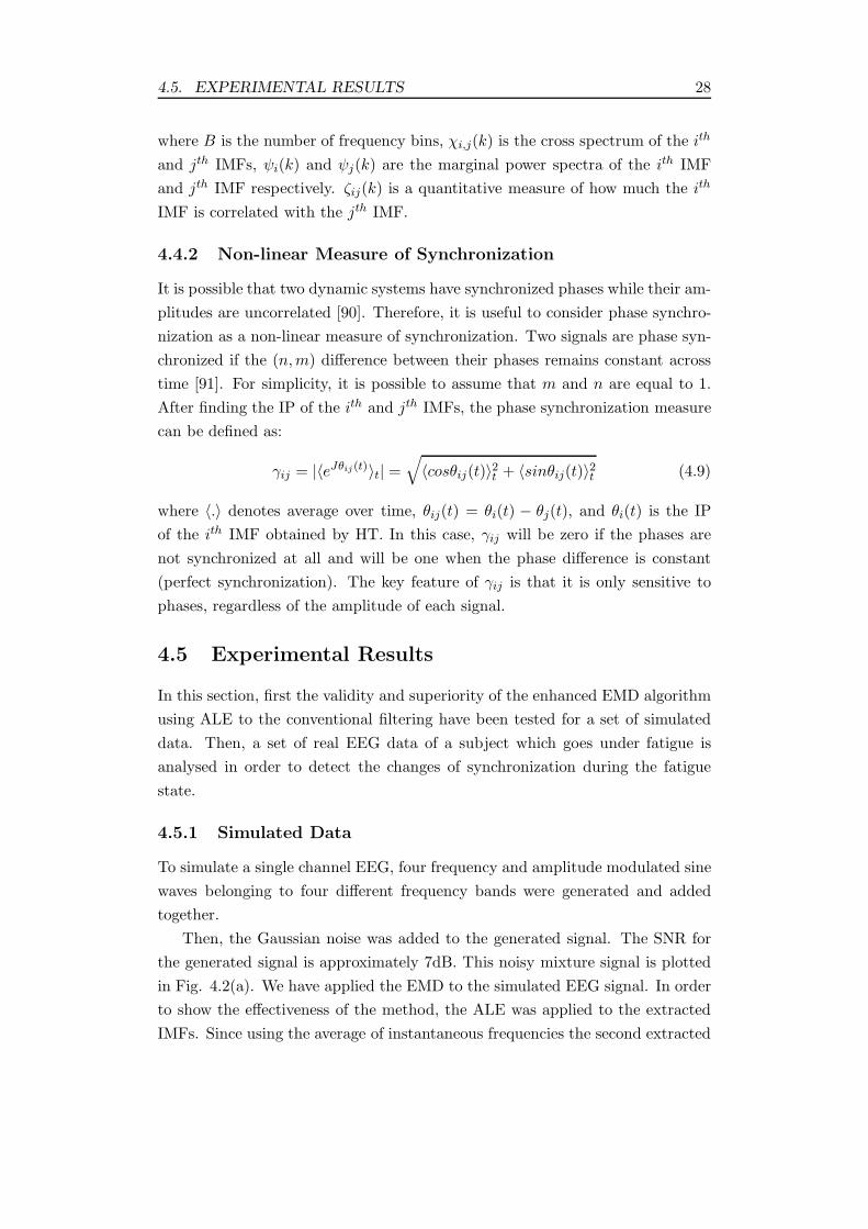
4.5. EXPERIMENTAL RESULTS 28
where B is the number of frequency bins, χi,j(k) is the cross spectrum of the ith
and jth IMFs, ψi(k) and ψj(k) are the marginal power spectra of the ith IMF
and jth IMF respectively. ζij(k) is a quantitative measure of how much the ith
IMF is correlated with the jth IMF.
4.4.2 Non-linear Measure of Synchronization
It is possible that two dynamic systems have synchronized phases while their am-
plitudes are uncorrelated [90]. Therefore, it is useful to consider phase synchro-
nization as a non-linear measure of synchronization. Two signals are phase syn-
chronized if the (n,m) difference between their phases remains constant across
time [91]. For simplicity, it is possible to assume that m and n are equal to 1.
After finding the IP of the ith and jth IMFs, the phase synchronization measure
can be defined as:
γij = |〈eJθij(t)〉t| =√
〈cosθij(t)〉2t + 〈sinθij(t)〉2t (4.9)
where 〈.〉 denotes average over time, θij(t) = θi(t) − θj(t), and θi(t) is the IP
of the ith IMF obtained by HT. In this case, γij will be zero if the phases are
not synchronized at all and will be one when the phase difference is constant
(perfect synchronization). The key feature of γij is that it is only sensitive to
phases, regardless of the amplitude of each signal.
4.5 Experimental Results
In this section, first the validity and superiority of the enhanced EMD algorithm
using ALE to the conventional filtering have been tested for a set of simulated
data. Then, a set of real EEG data of a subject which goes under fatigue is
analysed in order to detect the changes of synchronization during the fatigue
state.
4.5.1 Simulated Data
To simulate a single channel EEG, four frequency and amplitude modulated sine
waves belonging to four different frequency bands were generated and added
together.
Then, the Gaussian noise was added to the generated signal. The SNR for
the generated signal is approximately 7dB. This noisy mixture signal is plotted
in Fig. 4.2(a). We have applied the EMD to the simulated EEG signal. In order
to show the effectiveness of the method, the ALE was applied to the extracted
IMFs. Since using the average of instantaneous frequencies the second extracted
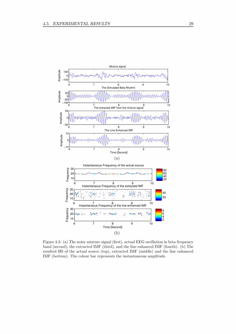
4.5. EXPERIMENTAL RESULTS 29
6 7 8 9 10−100
−50
0
50
Am
plit
ude
The Simulated Beta Rhythm 6 7 8 9 10
−100
0
100
Am
plit
ude
Mixture signal
6 7 8 9 10−50
0
50
Am
plit
ude
The extracted IMF from the mixture signal
6 7 8 9 10−10
0
10
Time [Second]
Am
plit
ude
The Line Enhanced IMF
(a)
Instantaneous Frequency of the extracted IMF
Fre
quency
6 7 8 9 10
10
20
30
20
40
Instantaneous Frequency of the line enhanced IMF
Time [Second]
Fre
quency
6 7 8 9 10
10
20
30
2468
Instantaneous Frequency of the actual source
Fre
quency
6 7 8 9 10
10
20
30
20406080
(b)
Figure 4.2: (a) The noisy mixture signal (first), actual EEG oscillation in beta frequencyband (second), the extracted IMF (third), and the line enhanced IMF (fourth). (b) Theresulted HS of the actual source (top), extracted IMF (middle) and the line enhancedIMF (bottom). The colour bar represents the instantaneous amplitude.
4.5. EXPERIMENTAL RESULTS 30
IMF belonged to the beta frequency band range around 20 Hz, we selected that
IMF as beta rhythm and plotted its HS in Fig. 4.2(b). From the HS it can be
seen that the IMF contains some wide-band components. We then applied the
ALE algorithm to the extracted IMF and computed the HS again and plotted
the results. Since a number of iterations are needed at the beginning for the
algorithm to converge, the ALE is applied to a window of longer size then the
resulted signal by the ALE is truncated. The HS of the actual EEG oscillation
in beta frequency band, extracted IMF, and the enhanced IMF are shown in
Fig. 4.2(b). From the plots in this figure it is evident that using the proposed
approach the wide-band noise has been reduced.
We calculated the correlation coefficient of the original simulated oscillation
with both the IMF and the enhanced IMF. In addition, we used a Butterworth
filter and a zero-phase filter of different degrees to filter the extracted IMF and
computed the correlation coefficients of the filtered IMF and the original oscilla-
tion. The highest correlation coefficient of 0.9137 was obtained by the IMF which
was filtered using the ALE. In the next section, we apply the enhanced EMD
algorithm to different channels and compute the synchronization measures of the
brain lobes before and during fatigue state in order to evaluate the corresponding
synchronization changes.
4.5.2 Real Data
The EEG data were recorded from participants who reported to be non-smokers,
to have normal sleep patterns, not to work night shifts, and not to use any pre-
scribed medication. From previous studies it is known that the participants
become more distracted by the information presented at irrelevant spatial lo-
cations with increasing mental fatigue (e.g. see [92]). Therefore, in each trial
a horizontal array of three uppercase letters was presented to the subjects in
which the central one was the relevant target letter and the remaining letters
were distractors. The participants were instructed to make a left-hand response
as quickly as possible if the target letter was an H and a right-hand response if
the central letter was an S and to ignore distractors. The letter array remained
on the screen until a response was given.
In the case that there was no response from the participants, the letter ar-
ray disappeared after 1200 ms. The focus of attention can be manipulated by
advance information [93]. To examine whether individuals still use available in-
formation to prepare for upcoming activities after a prolonged task performance,
an explicit cue was presented for 150 ms, 1000 ms before appearance of the three
letters specifying either the color of the target letter (the Dutch word for ‘red’
or ‘green’) or the response hand (the Dutch word for ‘left’ or ‘right’). The hand

4.5. EXPERIMENTAL RESULTS 31
and color cues were presented randomly with equal probability.
In half of the trials the distractors had the same identity and color as the
target letter (e.g., HHH or SSS: compatible) while in the other half of the trials
they had a different identity and color than the target letter (e.g., SHS or HSH:
incompatible). The stimuli of different types were presented randomly with
equal probability. During each trial a fixation mark remained visible on the
screen (an asterisk of 0.5 × 0.5 cm). The interval between the initial response
to one trial and the beginning of cue presentation on the following trial varied
randomly between 900 and 1100 ms. The subjects were instructed to have a fast
and accurate response and minimize the eye movements and blinking during the
task performance.
The task lasted as a two-hour experimental block without breaks preceded
by a practice block of 80 trials. EEG data was recorded from 22 scalp positions,
using Sn electrodes attached to an electrode cap. Electrode positions based on
extended 10-20 system were F7, F3, Fz, F4, F8, T7, C3, Cz, C4, T8, P7, P3,
Pz, P4, P8, O1, Oz, and O2. Additional intermediate positions were FC5, FC1,
FC2, and FC6. The electrodes were referenced to electronically linked earlobes.
Electro-oculograms (EOG) were recorded bipolarly with Sn electrodes from the
outer canthi of both eyes and from above and below the left eye. By adding gel,
electrode impedances were reduced to less than 5kΩ. The signals were lowpass
filtered with the cutoff frequency set at 30 Hz and sampled at a rate of 100 Hz.
Fifteen healthy young women with age ranging from 19 to 25 years partic-
ipated in the experiment. The EEG data of one of the subjects is selected.
Then, two separate segments of data from the first half an hour and last half an
hour are extracted. These segments are respectively, the representations of alert
and fatigue states. Each segment is analysed separately to measure the linear
synchronization (coherence) and non-linear synchronization (phase synchroniza-
tion) between the left and right hemispheres. F7, FC5, P7 channels from the left
hemisphere and F4, FC6, P8 from the right hemisphere are selected. The alpha
rhythm is extracted from F7 and F4, beta rhythm is extracted from FC5 and
FC6 and theta rhythm is extracted from P7 and P8. The overlapped windows
with the length of 4 seconds are considered for applying the HT and estimating
the coherence and phase synchronization.
Selection of the channels in each hemisphere for extracting each rhythm is
based on the HT of the resulted IMFs in several electrodes in the right and left
part of the brain. The IMF is selected from the channel that its resulted IMF
(in a certain frequency band) has frequency traces in time-frequency distribution
which are more continuous. Since the resulted beta rhythm was rather noisy,
the ALE was used to enhance it.

4.5. EXPERIMENTAL RESULTS 32
Alpha Coherence
Sample Number
Fre
quency
0 100 200 3000
5
10
15
20
25
30
0
0.2
0.4
0.6
0.8
1Theta Coherence
Sample Number
Fre
quency
0 100 200 3000
5
10
15
20
25
30
0
0.2
0.4
0.6
0.8
1
Alpha Coherence
Sample Number
Fre
quency
0 100 200 3000
5
10
15
20
25
30
0
0.2
0.4
0.6
0.8
1Theta Coherence
Sample Number
Fre
quency
0 100 200 3000
5
10
15
20
25
30
0
0.2
0.4
0.6
0.8
1
Sample Number
Fre
quency
Beta Coherence
0 100 200 3000
5
10
15
20
25
30
0
1
2
3
4
5
6x 10
−3
Sample Number
Fre
quency
Beta Coherence
0 100 200 3000
5
10
15
20
25
30
0
1
2
3
4
5
6x 10
−3
Figure 4.3: Interhemisphere coherence of beta, alpha and theta rhythms, the top rowcorresponds to the fatigue state and the bottom row corresponds to the alert state.
The results of the estimated coherence and phase synchronization values for
the two segments of the data are shown in Fig. 4.3 and Fig. 4.4. The algorithm
is repeated over more trials for alert and fatigue states. Approximately, in all of
the trials the coherence of beta rhythms between the left and right hemisphere
decreases and the coherencies for alpha and theta rhythms increase from the alert
to fatigue state. The estimated phase synchronization values between rhythms
have been shown to be different across different trials especially for theta rhythm.
However in most trials, the phase synchronization of beta rhythms decreases
while for alpha rhythms it increases from the alert to fatigue state.
In addition, we measured the phase synchronization and coherence around
stimulus onset before and during fatigue state. Since the segment of data around
stimulus onset is considered for measuring phase synchronization and coherence,
the length of the data segment is reduced to only one second before stimulus
onset and one second after stimulus onset. However for applying the EMD a
longer window size is considered while for measuring phase synchronization the
window size is reduced since the timing between the consecutive stimuli is very
short (from 1 second to 2 seconds).
We considered 3 seconds of the data segment after stimulus onset and applied
the EMD. For beta rhythm, ALE is applied to the resulted IMF. One second

4.5. EXPERIMENTAL RESULTS 33
0 100 200 3000
0.2
0.4
0.6
0.8
1
Sample Number
Synchro
niz
ation V
alu
e
Alpha Synchronization
0 100 200 3000
0.2
0.4
0.6
0.8
1
Sample Number
Synchro
niz
ation V
alu
e
Theta Synchronization
0 100 200 3000
0.2
0.4
0.6
0.8
1
Sample Number
Synchro
niz
ation V
alu
e
Beta Synchronization
During Fatigue
Before FatigueBefore Fatigue
During Fatigue
Before Fatigue
During Fatigue
Figure 4.4: Interhemisphere phase synchronization of beta (left), alpha (middle), andtheta (right) rhythms.
of data segment before stimulus onset and one second after stimulus onset are
considered for measuring phase synchronization. Beta and theta rhythms are
extracted from F3 and F4 channel and alpha rhythm is extracted from C3 and
C4 channels. The phase synchronization is measured for five trials one second
before and after stimulus onset. The results are shown in Fig. 4.5. The aver-
aged phase synchronization is also depicted as the thick line. From these figures
it can be seen that the best discrimination is obtained considering phase syn-
chronization of the alpha rhythm. Also as the frequency of the rhythm decreases
(e.g. from beta to theta rhythm) the variance of the consecutive measured phase
synchronization across time increases. The coherence of beta, alpha, and theta
rhythms are measured around the stimulus onset for five trials and the averaged
coherence for all the rhythms are shown in Fig 4.6, Fig 4.7 and Fig 4.8.
It can be seen from these figures that there is not a good discrimination
in coherence before and during fatigue state. Therefore, considering the above
experiments, the window length size plays an important role. Reduced window
length size (e.g. one second) is not effective when measuring coherence. The best
discrimination with respect to phase synchronization is obtained for the alpha
rhythm. However all the phase synchronization measures can have an important
role for detecting the fatigue state. This can be done by selecting a regression or a
classification method and using the extracted phase synchronization in different
frequency bands from different regions of the brain. The coherence measure, if
included, should not be considered around the stimulus onset and the window
size should not be small (e.g. one second).
In the next section, a new method is developed for estimation and tracking
the IP of the EEG oscillations. This method is in the initial stage and should be
improved in the future to be applied for estimation of EEG phase synchronization
with application to mental fatigue analysis.

4.5. EXPERIMENTAL RESULTS 34
0 20 40 60 80 100 120 140 160 180 2000
0.2
0.4
0.6
0.8
1
Time [Sample number]
Phase s
ynchro
niz
ation
Beta phase synchronization (F3−F4)
after stimulus − during fatigue
before stimulus − during fatigue
after stimulus − before fatigue
before stimulus − before fatigue
0 20 40 60 80 100 120 140 160 180 2000
0.2
0.4
0.6
0.8
1
Time [Sample number]
Phase s
ynchro
niz
ation
Theta phase synchronization (F3−F4)
before stimulus − before fatigue
before stimulus − during fatigue
after stimulus − before fatigue
after stimulus − during fatigue
0 20 40 60 80 100 120 140 160 180 2000
0.2
0.4
0.6
0.8
1
Time [Sample number]
Phase s
ynchro
niz
ation
Alpha phase synchronization (C3−C4)
after stimulus − before fatigue
before stimulus − during fatigue
before stimulus − before fatigue
after stimullus − during fatigue
Figure 4.5: Phase synchronization of beta (top), alpha (middle), and theta (bottom)rhythms around stimulus onset.

4.5. EXPERIMENTAL RESULTS 35
before stimulus − before fatigue
Time [sample number]
Fre
quency
0 20 40 60 80 1000
5
10
15
20
25
30
0
0.2
0.4
0.6
0.8
1
after stimulus − before fatigue
Time [sample number]
Fre
quency
0 20 40 60 80 1000
5
10
15
20
25
30
0
0.2
0.4
0.6
0.8
1
before stimulus − during fatigue
Time [sample number]
Fre
quency
0 20 40 60 80 1000
5
10
15
20
25
30
0
0.2
0.4
0.6
0.8
1
after stimulus − during fatigue
Time [sample number]
Fre
quency
0 20 40 60 80 1000
5
10
15
20
25
30
0
0.2
0.4
0.6
0.8
1
Alpha coherence C3−C4
Figure 4.6: Coherence of alpha rhythm around stimulus onset for before fatigue (toprow) and during fatigue (bottom row). Dark blue colour presents lack of coherence anddark red colour presents the maximum coherence.

4.5. EXPERIMENTAL RESULTS 36
before stimulus − before fatigue
Time [sample number]
Fre
quency
0 20 40 60 80 1000
5
10
15
20
25
30
0
0.2
0.4
0.6
0.8
1
after stimulus − before fatigue
Time [sample number]
Fre
quency
0 20 40 60 80 1000
5
10
15
20
25
30
0
0.2
0.4
0.6
0.8
1
before stimulus − during fatigue
Time [sample number]
Fre
quency
0 20 40 60 80 1000
5
10
15
20
25
30
0
0.2
0.4
0.6
0.8
1
after stimulus − during fatigue
Time [sample number]
Fre
quency
0 20 40 60 80 1000
5
10
15
20
25
30
0
0.2
0.4
0.6
0.8
1
Beta coherence F3−F4
Figure 4.7: Coherence of beta rhythm around stimulus onset for before fatigue (top row)and during fatigue (bottom row). Dark blue colour presents lack of coherence and darkred colour presents the maximum coherence.

4.5. EXPERIMENTAL RESULTS 37
before stimulus − before fatigue
Time [sample number]
Fre
quency
0 20 40 60 80 1000
5
10
15
20
25
30
0
0.2
0.4
0.6
0.8
1
after stimulus − before fatigue
Time [sample number]
Fre
quency
20 40 60 80 100
5
10
15
20
25
30
0
0.2
0.4
0.6
0.8
1
before stimulus − during fatigue
Time [sample number]
Fre
quency
0 20 40 60 80 1000
5
10
15
20
25
30
0
0.2
0.4
0.6
0.8
1after stimulus − during fatigue
Time [sample number]
Fre
quency
0 20 40 60 80 1000
5
10
15
20
25
30
0
0.2
0.4
0.6
0.8
1
Theta coherence F3−F4
Figure 4.8: Coherence of theta rhythm around stimulus onset for before fatigue (toprow) and during fatigue (bottom row). Dark blue colour presents lack of coherence anddark red colour presents the maximum coherence.

4.6. INSTANTANEOUS PHASE TRACKING OF EEG OSCILLATIONS
USING EMD AND RBPF 38
4.6 Instantaneous Phase Tracking of EEG Oscilla-
tions using EMD and RBPF
In this section, a new method for IP tracking of oscillatory signals in a narrow
band frequency range is proposed. EMD as an adaptive and data-driven method
for analysing non-linear and non-stationary time series, is applied to a mixture
of signals. Then, one of the resulted IMFs is used for estimating the IP of the
signal in a certain frequency band.
Since by applying EMD to the noisy signal, the noise is distributed over
the IMFs, the RBPF is used to track the actual IP of the noisy IMF. The
formulated RBPF operates based on smoothing the IF traces in Hilbert domain
and denoising the signal in time domain. Finally, the method is able to track the
IP across consecutive time points. The method is applied to both simulated and
real data. As an application, in future it can be used for mental fatigue analysis
based on the changes in phase synchronization of different brain rhythms in
different brain regions before and during the fatigue state.
Decomposition of signals into their constituent oscillatory components has
wide applications in various fields. This may be efficiently performed using EMD
and often to restore the resulted IMFs from noise. As stated in the first section
of this chapter, in some previous research conventional filtering is suggested for
removing the noise from the IMF which usually results in deteriorating the phase
information. In [94] a number of EMD-based denoising inspired by the standard
wavelet thresholding is proposed. In the previous section ALE was proposed
and applied to the IMF in order to enhance and de-noise it. HT is then used
for estimation of IP. In this section we propose a new method based on RBPF
in order to directly estimate the IP of the IMF. The method can be used as a
general de-noising algorithm but the focus in this section is to estimate the IP
from the noisy IMF. Since the algorithm requires setting a few parameters, for
measuring phase synchronization using the proposed method, the parameters
should be selected carefully.
EMD is applied to the EEG signal in order to extract its different oscillations.
Our proposed method in the first step uses the EMD in order to decompose
the EEG into the IMFs. The method tries to smooth the frequency traces
in Hilbert domain and estimate the phase. In the next subsections, first the
problem formulation using RBPF is provided and then the simulation and real
data results are presented.

4.6. INSTANTANEOUS PHASE TRACKING OF EEG OSCILLATIONS
USING EMD AND RBPF 39
4.6.1 Problem Formulation using RBPF
Suppose that EMD is applied to the mixture signal x to decompose it to its
corresponding IMFs. Then the HT is used to compute the analytic signal for
the IMFs (having the IMF as the real part and its HT as the imaginary part,
see equation (4.4)) as:
dt(i) + JHd[dt(i)] = at(i)eJθt(i) i = 1, ...,M (4.10)
where J =√−1 and at(i) and θt(i) are the IA and IP of the ith IMF respectively,
Hd[.] denotes the HT, and M is the number of IMFs. Then, the mixture signal
can be reconstructed as:
x(t) =M∑
i=1
dt(i) = Real(M∑
i=1
at(i)eJθt(i)) (4.11)
Now, it is possible to formulate the IA and IP of each IMF as the state variables
of the PF [83] and the mixture signal as the observation. Therefore, the state
transition and observation equations of the PF can be expressed as:
ρt = [θt(1) at(1) . . . θt(M) at(M)] (4.12)
ρt = f(ρt−1) + wt−1 (4.13)
x(t) = G(ρt) + vt (4.14)
where x(t) is the mixture signal, vt,wt−1 are WGN with known covariance ma-
trices Qvt and Qw
t−1 respectively, M is the number of IMFs and
G(ρt) = Real(M∑
i=1
at(i)eJθt(i)) (4.15)
From the above equations it can be seen that it is possible to partition the
state variables into linear and non-linear parts. Therefore, we formulate the
problem using the concept of RBPF [85]. The RBPF marginalizes out the linear
state variables in order to reduce the size of the state space. Therefore, a reduced
number of particles are required for the RBPF to achieve the same performance
as for the PF. We rewrite equation (4.12) as:
ρt = [ρ1t ρ
2t ] (4.16)
ρ1t = [θt(1) . . . θt(M)] (4.17)
ρ1t = [at(1) . . . at(M)] (4.18)

4.6. INSTANTANEOUS PHASE TRACKING OF EEG OSCILLATIONS
USING EMD AND RBPF 40
where ρ1t is the non-linear state variable and ρ
2t is the linear state variable.
Then, the state transition and observation equations can be written in the vector
form as:
ρt = f(ρt−1) + wt−1
x(t) = G(ρt) + vt
G(ρt) = ρ2tG
′(ρ1t )
= [at(1) . . . at(M)]
Real(eJθt(1))
. . .
Real(eJθt(M))
(4.19)
ρ2t is estimated using KF [83] and ρ
1t is estimated by PF. Considering the above
equations, if the state transition function f were available, it would be possi-
ble to track the IA and IP of each IMF and de-noise the mixture signal using
RBPF. However, the state transition function is not known and especially for
phase it cannot be modelled simply using a Markov process. Therefore, first we
utilize the RBPF in order to formulate the problem and then several equations
and constraints are employed to the RBPF algorithm in order to track the IP
effectively.
Here we focus on the phase tracking from one IMF. In future, the method
can be extended to track the IP and IA of multiple IMFs at each time point.
Suppose that we applied EMD to one channel of EEG signal as x(t). Usually
the first and second IMFs are noisy since they contain the highest frequency
available in the signal. If we compute the analytic signal using equation (4.10),
the IF of the IMF can be estimated using derivative of the phase (see equation
(4.5)). In the following it is shown that for the noisy IMF, the frequency trace
across time points is not smooth and the effect of wide band noise can be clearly
seen when there is a jump in the estimated IF of the time samples. We select
the ith IMF which is noisy. Therefore, the state variables, state transition, and
observation function can be considered as:
ρt(i) = [θt(i) at(i)], ρ1t (i) = θt(i), ρ
2t (i) = at(i) (4.20)
ρt(i) = f(ρt−1(i)) + wt−1
imft(i) = G(ρt(i)) + vt
G(ρt(i)) = at(i)Real(eJθt(i))
(4.21)
Our proposed method tries to smooth the IF traces in Hilbert domain and then

4.6. INSTANTANEOUS PHASE TRACKING OF EEG OSCILLATIONS
USING EMD AND RBPF 41
estimate the IP using the information provided by the IF. Each IMF belongs
to a specified frequency band. So, it is possible to determine the minimum and
maximum frequencies for the band in which IMF belongs to. By generating
some simulated signals, applying the EMD, and evaluating the IP of the IMF
using HT, it is evident that the phase sign suddenly changes across time points.
However, if we consider the absolute value of the phase, the phase change is not
significant. The IA is smooth across all time samples.
As shown in equation (4.20), we formulated the phase as the non-linear state
variable and the amplitude as the linear state variable of the RBPF. Both of
them are considered as the Markov process. We also save one variable as the
estimated IF. This variable does not have a direct role in estimating the phase,
however it is useful in updating the weight of some particles and deciding on
the phase transition. When we generate new particles corresponding to the
IP from the previous time point, we need to generate two phases. One phase
is obtained from the phase in the previous time sample plus the state noise.
Another phase is obtained from the negative of the phase in the previous time
sample plus noise. Then, we calculate IFs for both generated phases. We select
the generated phase in which the estimated IF smooths the frequency traces
across time samples (using the stored IF estimate in the previous time point).
When we tried to test and develop the method using simulated signal, there
was a situation that the phase in one time sample was close to zero and the
phase in the next time sample was also close to zero. In this case the calculated
frequency went out of the frequency range and became negative in the later
time samples. Although in consecutive time points, the IF traces return to the
actual track before becoming negative or going beyond the frequency range. In
this situation the method is not able to distinguish the correct generated phase
based on the frequency traces. We used some if-then-rules and detected the
situation that the estimated phase is close to zero. Therefore in that situation
the phase selection stems from considering the observation and the estimated
amplitude by KF.
Before deciding on the generated phase (from positive/negative of the phase
in previous time sample) we estimate the IA for both generated phases using
KF. We update the weight of each particle using two scales. One scale relates to
the frequency transition, the other scale relates to the weight given by using the
observation and the amplitude estimated by KF. In the case where the generated
frequency is out of band but still is a valid frequency and not related to noise
(i.e. due to the phase transition around zero), we estimate another frequency
from previous time point in order not to lose the frequency track.
Therefore, we cannot have an equivalent scale for frequency transition like

4.6. INSTANTANEOUS PHASE TRACKING OF EEG OSCILLATIONS
USING EMD AND RBPF 42
the case that frequency is inside the specific band. However, we set the second
scale equal to 1 to have better phase transition. Then, we select the generated
phase in which the estimated weight is higher. We do not store the generated
frequency which is negative or out of the frequency band. Instead, we generate
a new frequency which is equal to the stored frequency in the previous time
sample plus a Gaussian random generated number. In this case we do not lose
the frequency track inside the band in the later time points and have better
phase transition near zero.
In addition, our method involves some constraints. When the selected phase
is larger than π or smaller than −π the weight of the particle will be set to zero
in order not to have any contribution to the estimation of the posterior density.
In addition, when the estimated frequency is out of the frequency band range,
we set the weight of that particle to zero.
The pseudo-code of the proposed method for IP tracking of one IMF is shown
in Algorithm 4.1. τ is the threshold to determine when the phase transition is
near zero. In our simulation this was set to 0.15. We consider a window of
length T + 1 and apply the EMD. After one noisy IMF is selected, the HT is
applied to that IMF. We use the estimated IF, IP, and IA of the noisy IMF
at the first time point and initialize the particles. This initialization moves the
particles into the right part of posterior density and is helpful to speed up the
convergence of the RBPF. The method is applied to the rest of T time samples.

4.6. INSTANTANEOUS PHASE TRACKING OF EEG OSCILLATIONS
USING EMD AND RBPF 43
Algorithm 4.1 Pseudo-code for phase tracking of one IMF
select ith IMF as dt(i), n = 1, ..., Ns, Nsis the number of particles.
set t = 0 and generate random numbers θ(n)0 ,freq
(n)0
according to random uniform distribution considering the HT of the IMF.
Initialize σ, σ1, minf , maxf , Ts (Sampling period), τ
for t = 1 to tmax tmax is the number of all time samples- generate random numbers w
ρ(n)1t−1 ,w
ρ(n)2t−1 and q
ρ(n)t−1
- set θ(n)t = θ
(n)t−1 + w
ρ(n)1t−1
- set θ(n)t = −θ(n)
t−1 + wρ(n)2t−1
- Calculate freq1 = diff (unwrap [θ(n)t−1 θ
(n)t ])/Ts/(2 × π)
- Calculate freq2 = diff (unwrap [θ(n)t−1 θ
(n)t ])/Ts/(2 × π)
- Estimate frequency freq = freq(n)t−1 + q
ρ(n)t−1
- Set θ(n)t as the phase, estimate amplitude a
(n)1t by Kalman filtering
- Set f1 = a(n)1t ×Real(eJθ
(n)t ),
ws1 = exp (−(dt(i) − f1) × (dt(i) − f1)/(2 × σ21))
- Set θ(n)t as the phase, estimate amplitude a
(n)2t by Kalman filtering
- Set f2 = a(n)2t ×Real(eJθ
(n)t ),
ws2 = exp (−(dt(i) − f2) × (dt(i) − f2)/(2 × σ21))
- if (|θ(n)t | < τ and |θ(n)
t−1| < τ) or (|θ(n)t | < τ and |θ(n)
t−1| < τ)
weight1 = ws1, weight2 = ws2
freq1 = freq , freq2 = freq, ws1 = 1, ws2 = 1
- else
-weight1 = exp (−(freq − freq1) × (freq − freq1)/(2 × σ2))
-weight2 = exp (−(freq − freq2) × (freq − freq2)/(2 × σ2))
- end if
- if weight1 > weight2
θ(n)t = θ
(n)t ,a
(n)t = a
(n)1t , freq
(n)t = freq1, w
(n)t = w
(n)t−1 × ws1 × weight1
- else
θ(n)t = θ
(n)t ,a
(n)t = a
(n)2t , freq
(n)t = freq2, w
(n)t = w
(n)t−1 × ws2 × weight2
- end if
- if (θ(n)t > π) or (θ
(n)t < −π) w
(n)t = 0
- if (freq(n)t > maxf ) or (freq
(n)t < minf ) w
(n)t = 0
- Normalize particle weights w(n)t = w
(n)t /
∑Nn=1(w
(n)t )
- Resample
- end for

4.6. INSTANTANEOUS PHASE TRACKING OF EEG OSCILLATIONS
USING EMD AND RBPF 44
4.6.2 Application
4.6.2.1 Simulated Results
Four frequency and amplitude modulated sine waves which belong to four differ-
ent frequency bands are generated and WGN is added to sum of the sine waves.
The available signal to noise power is measured by SNR in dB unit which is
defined as:
SNR = 10log10(Psignal
Pnoise) (4.22)
We generated two simulated signals in which the SNR for the first and second
signal obtained as 3.0445dB and 7.2167dB respectively. Next, the EMD method
is applied to decompose the generated signals into a number of IMFs. In both
simulated signals, the second IMF belonged to the frequency range around 20Hz.
Since, the resulted IMF was noisy, the proposed method in this section is applied
to the IMF in order to track the actual IP of the signal in the frequency range
around 20Hz.
We computed the IP, IA, and IF of the actual generated sine wave using HT.
Then, we compared the results of tracking the IP, IA, and IF using our method
with the results obtained by the HT applied to the noisy IMF. The results are
provided in Fig. 4.9 and Fig. 4.10. The mean square error (MSE) of the phase is
calculated using the following equation and is shown in Table 4.1 for both SNR
levels.
MSE = 1/T
T∑
t=1
(θestimate(t) − θactual(t))2 (4.23)
where T is the number of time samples. It can be seen from Fig. 4.10 that
around the 10th time sample (the corresponding phase in Fig. 4.9 is around
0) the actual frequency decreases, becomes negative, and then it returns to the
previous track. However, our method can detect these changes in frequency
which is not related to the noise and smooths the frequency such that it does
not much affect the phase estimation. Therefore, in this case although we cannot
estimate the actual frequency we keep the frequency in a track that will not be
lost inside the specified frequency band and it can remove the wide-band noise
in other time points as well. In addition, since the estimated frequency does not
Table 4.1: MSE of the phase in two SNR levels.
SNR=3.0445dB SNR=7.2167dB
Proposed method 3.7634 2.6952
HT of the noisy IMF 5.7522 3.5871

4.6. INSTANTANEOUS PHASE TRACKING OF EEG OSCILLATIONS
USING EMD AND RBPF 45
0 20 40 60 80 100−4
−2
0
2
4
Time [Sample]
Ph
ase
Instantaneous phase (IP) estimation (SNR=3.0445dB)
Actual IP
IP of the noisy IMF
IP tracking using RBPF
0 20 40 60 80 100−4
−2
0
2
4
Time [Sample]
Ph
ase
Instantaneous phase (IP) estimation (SNR = 7.2167 dB)
Actual IP
IP of the noisy IMF
IP tracking using RBPF
0 20 40 60 80 1000
20
40
Time [Sample]
Am
plit
ud
e
Instantaneous amplitude (IA) estimation (SNR=3.0445dB)
Actual IA
IA of the noisy IMF
IA tracking using RBPF
0 20 40 60 80 1000
20
40
Time [Sample]
Am
plit
ud
e
Instantneous amplitude (IA) estimation (SNR=7.2167dB)
Actual IA
IA of the noisy IMF
IA tracking using RBPF
Figure 4.9: IP (top two rows) and IA (bottom two rows) estimation using the proposedand HT methods in two SNR levels.
have direct impact on phase estimation, still the phase estimation around zero is
very promising. It can be seen from the figures that when the SNR is lower, the
error in estimation is higher. However the overall performance of the method
depends also on the operation of EMD.
4.6.2.2 Real Data Results
The real EEG data of a subject in a continuous visual experiment, explained
in Section 4.5.2, is used to apply the proposed phase tracking method. Using
lowpass interpolation algorithm the sampling frequency was increased to 200Hz.
The corresponding algorithm is explained in [95]. We selected the C3 channel
and applied the EMD algorithm. The first IMF belonging to beta frequency
range was selected and the method applied. The results are provided in Fig.
4.11 and Fig. 4.12.
Therefore, the new proposed phase tracking method uses the IMF given
by the EMD algorithm in order to remove the wide-band noise by applying
a constrained version of RBPF. As a result, the frequency traces of the IMF
become smoother and a better estimation for the IP is achieved. The proposed
method is very demanding in order to better estimate the IP of the beta rhythm
of the EEG signal, which is usually noisy and contains wide-band noise. The
changes in phase synchronization of beta rhythm among different brain regions

4.7. CONCLUSIONS 46
0 20 40 60 80 100−20
0
20
40
60
80
Time [Sample]
Fre
qu
en
cy [
Hz]
Instantaneous Frequency (IF) estimation by different methods (SNR = 3.0445dB)
0 20 40 60 80 100−20
0
20
40
60
80
Time [Sample]
Fre
qu
en
cy [
Hz]
Instantaneous Frequency (IF) estimation by different method (SNR = 7.2167dB)
Actual IF
IF of the noisy IMF
IF smoothing using RBPF
Actual IF
IF of the noisy IMF
IF smoothing using RBPF
Figure 4.10: IF estimation using the proposed (dotted line) and HT (bold red line)methods in two SNR levels of 7.2dB (top) and 3dB (bottom).
before and during fatigue state, can play an important role in analysis of mental
fatigue. Another application of the method is in speech analysis. When the EMD
is applied to speech signals, the noise at each time point will be distributed to the
IMFs. Therefore, for enhancing several IMFs simultaneously and de-noising the
speech signal at each time point, the method should be extended and effectively
applied. Further, the method can be developed more in order to solve the mode
mixing problem in the EMD algorithm.
4.7 Conclusions
In this chapter a new approach for mental fatigue analysis is presented which
considers synchronization of brain lobes in different frequency bands. In order
to measure the synchronization, the EEG oscillations are extracted from the
EMD algorithm. Because often the first few extracted IMFs contain noise, it
is suggested to enhance the IMFs by using an ALE. By applying the proposed
method to the EEG data of a subject which goes under fatigue, changes in the
coherence and phase synchronization of the left and right brain hemispheres in
different frequency bands are detected.
In addition, a new method based on RBPF is proposed for IP estimation
of an oscillatory waveform. The proposed method can be used for measuring
phase synchronization of two oscillations in mental fatigue analysis. However
since the method uses RBPF and several constraints and parameters, there is
a need for optimal selection of the parameters. Therefore, the method needs to
be improved in future for more reliable analysis of mental fatigue based on the
changes in the estimated phase synchronization. In the next two chapters, two
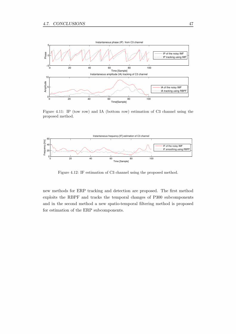
4.7. CONCLUSIONS 47
0 20 40 60 80 100−5
0
5
Time [Sample]
Phase
Instantaneous phase (IP) from C3 channel
0 20 40 60 80 1000
5
10
Time[Sample]
Am
plit
ude
Instantaneous amplitude (IA) tracking of C3 channel
IA of the noisy IMF
IA tracking using RBPF
IP of the noisy IMF
IP tracking using IMF
Figure 4.11: IP (tow row) and IA (bottom row) estimation of C3 channel using theproposed method.
0 20 40 60 80 1000
20
40
60
Time [Sample]
Fre
qu
en
cy [
Hz]
Instantaneous frequency [IF] estimation of C3 channel
IF of the noisy IMF
IF smoothing using RBPF
Figure 4.12: IF estimation of C3 channel using the proposed method.
new methods for ERP tracking and detection are proposed. The first method
exploits the RBPF and tracks the temporal changes of P300 subcomponents
and in the second method a new spatio-temporal filtering method is proposed
for estimation of the ERP subcomponents.

Chapter 5
Coupled RBPF for Single Trial
Estimation of ERPs in
Temporal Domain with
Application to Mental Fatigue
5.1 Introduction
In this chapter a new method for investigating mental fatigue based on P300
variability is presented. Based on this approach a new coupled PF for tracking
variability of P300 subcomponents i.e. P3a and P3b, is developed for single trial
recordings. Some research has been carried out using BSS and PCA for decom-
position of P300 into its subcomponents [69, 75, 76, 77, 78]. In some studies
PCA has been applied to the averaged ERP [79, 80, 81]. The PCA method
used in these studies is suitable for stationary data disregarding their trial-to-
trial variations. The major problem with these methods is that when there is a
high temporal correlation between the subcomponents, low signal to noise ratio
ERPs, or correlated noise, they may fail to produce correct results. In some
cases they are able to estimate only one of the subcomponents. A recent work
for single trial estimation of ERP components in [68] formulates wavelet coeffi-
cients of the time-locked measured ERPs in the state space and then estimates
the ERP components using PF. It is shown that the formulated PF outper-
forms KF. The method however fails to estimate ERP subcomponents (such as
P300 subcomponents). Therefore, a new modelling of ERP subcomponents is
demanded.
48

5.1. INTRODUCTION 49
In this chapter we propose a method based on RBPF [85] to track the dy-
namic changes of the amplitude, latency, and shape of P300 subcomponents
across trials. The proposed method considers the temporal correlation between
P300 subcomponents recorded from different sites of the brain and enables sep-
aration and identification of the subcomponents. The latency, amplitude, and
width of each subcomponent, as the main varying parameters, are modelled us-
ing state space systems. In this model the observation is modelled as a linear
function of amplitude and a non-linear function of latency and width. Because
of uncertainty in the estimation and tracking, two RBPFs are coupled and em-
ployed for recursive estimation of the system state across trials. By including
some physiological based constraints, the proposed technique prevents genera-
tion of invalid particles during estimation of the state.
The main advantage of the algorithm compared with other single trial based
methods is its robustness to low signal-to-noise ratios and temporal correlation
between the P300 subcomponents. The method is applied to both simulated data
and real mental fatigue data to track subtle changes of the P300 subcomponents
before and during fatigue state. The results demonstrate potential use of the
method in ERP based applications.
Some preliminary results of the method have been presented in [96]. The
method presented in this chapter can be considered as an extension of our pre-
vious work in [97], in which a constrained PF was employed for separation and
tracking the P300 subcomponents from only a single channel.
The designed coupled RBPF (CRBPF) has shown to be helpful and effective
in single trial estimation of P300 subcomponents and it can be employed for
single trial estimation of any other ERP subcomponents using the corresponding
physiological based constraints. The concept of the designed CRBPF is novel
and it is expected to be used in some applications where synchronous tracking
of states of two dependent systems is required.
The remainder of this chapter is structured as follows. In Section 5.2, a PF
formulation is developed for estimation of ERP subcomponents from single trial
EEG signals. Then, in Section 5.3, the CRBPF is proposed to track variations
of P300 subcomponent across different single trials. In Section 5.4 the method
is first applied to simulated data and then it is applied to real mental fatigue
data. Finally, Section 5.5 concludes the chapter.
5.2. PROBLEM FORMULATION USING PF 50
5.2 Problem Formulation using PF
In order to track the variations of P3a and P3b parameters within consecutive
time-locked trials of stimulated EEGs, PF can be effectively used. Since the aim
is to track the latency, amplitude, and width of the ERP subcomponents across
trials, the state vector of the PF can be formed as:
xk = [ak(1) bk(1) sk(1) . . . ak(p) bk(p) sk(p)]T (5.1)
where ak(i) is the amplitude, bk(i) is the latency, and sk(i) is the width of the ith,
i = 1, ..., p, subcomponent in the kth trial, and p is the number of subcomponents.
Based on the above definitions the state transition and observation equations are
expressed as:
xk = xk−1 + nk−1 (5.2)
zk = f(t;xk) + vk (5.3)
where zk is the time-locked single trial measurement and
f(t;xk) = f(t;ak,bk, sk) =
p∑
i=1
ak(i)e−
(t−bk(i))2
2s2k(i) for i = 1, ..., p (5.4)
Here t denotes the time index and varies from the beginning of the ERP com-
ponent to the end of ERP component. The whole time samples in a vector
format [f(1;xk) ... f(T;xk)] are used in the observation equation. Based on this
model, each ERP component is modelled as sum of its subcomponents and each
subcomponent is approximated by a Gaussian waveform.
In many studies (e.g. see [98, 99]) P300 subcomponents are modelled using
parametric functions. Among them Gaussian waveform is the most commonly
used type for modelling such subcomponents [82]. Although the actual ERP
subcomponents are not necessarily exactly Gaussian waveforms but modelling
them as Gaussians leads to a robust and fast estimation of the peak parameters
(latency and amplitude). This is what neurophysiologists and cognitive scientists
are primarily concerned with.
Using the concept of PF, the available measurements for tracking variabil-
ity of ERP subcomponents are time-locked single trials. The aim of tracking
is to recursively estimate the state of the system which contains the latency,
amplitude, and width of each ERP subcomponent.

5.3. COUPLED RBPF FORMULATION 51
5.3 Coupled RBPF Formulation
The objective here is to incorporate the topographic information of P3a and
P3b (locations) into the detection and tracking algorithm which can interlink
two trackers corresponding to P3a and P3b to work together. In this section the
problem of tracking ERP subcomponents using RBPF from a single channel is
formulated first and then the required conditions and measures for coupling two
RBPFs, in order to track P300 subcomponents, are described.
It can be seen from equation (5.4) that each ERP component is modelled
as sum of several Gaussian waveforms representing its subcomponents. It is
possible to factorize the observation model into amplitude information (as the
linear part) and exponentially varied waves (as the non-linear part). In this case
a linear relation between the observation and the vector of amplitudes has been
made while there is generally a non-linear relation with respect to other state
variables.
Regarding equations (5.1)–(5.4) and using the concept of RBPF, the state-
space and observation can be formulated respectively as:
x1k = [bk(1) sk(1) . . . bk(p) sk(p)]
T (5.5)
x2k = [ak(1) . . . ak(p)]
T (5.6)
zk = [f1(t;x1k) . . . fp(t;x
1k)][ak(1) . . . ak(p)]
T + vk (5.7)
where as in (5.4)
fi(t;x1k) = fi(t; bk(i), sk(i)) = e
−(t−bk(i))2
2s2k(i) for i = 1, ..., p (5.8)
According to the concept of RBPF, the state vector is partitioned into the vectors
of linear and non-linear variables. Based on equations (5.5) and (5.6), x1k is
the non-linear state vector which contains non-linear variables and x2k is the
linear state vector which contains the linear variables. Comparing the above
equations with equations (3.20), (3.21) and (3.22), it is evident that Ck(x1k) (in
equation (3.22)) is modelled as the matrix of exponentials fi(t; bk(i), sk(i)) which
contains the non-linear state variables (latency and width). Also for simplicity
Bk−1(x1k−1) (in equation (3.21)) is selected as the unitary matrix. In this case the
state transition for the linear state variables is independent from the non-linear
state variables.
It is possible to apply the RBPF to the single channel of the time-locked mea-
sured ERPs in order to track the dynamic changes in latency, amplitude, and
width of ERP subcomponents. In the initialization stage, instead of generating

5.3. COUPLED RBPF FORMULATION 52
random particles, we can use the averaged ERP of several consecutive trials and
generate some particles which contribute more to the posterior density. In the
subsequent trials, due to the existence of noise and artefact in the data, the
correct track of ERP subcomponent parameters may be lost. The use of some
physiological constraints on the state variables can be helpful in order to remove
the particles which are invalid while they have contribution to the estimation of
posterior density. The constraints can be set using the prior knowledge about the
ERP subcomponent specifications. In addition, it is possible to apply the track-
ing procedure to more channels and impose more meaningful constraints. Here,
we have designed the CRBPF for tracking the variability of P300 subcompo-
nents from two channels. The subcomponents (P3a and P3b) can be considered
spatially disjoint, however they usually overlap temporally on the scalp [22].
As we mentioned in Chapter 2, Section 2.2.1, P3a is located more towards
the frontal site while P3b is located more towards the parietal part of the brain.
Hence, P3a has larger amplitude over the frontal electrodes and P3b has larger
amplitude over the parietal electrodes. In addition, the electrodes on midline
are found to be more effective in detection of P300 [22]. We then select Fz
electrode in the frontal and Pz electrode in the parietal site. Two RBPFs are
formulated. The first one (RBPF1) is applied to the Fz channel while the second
one (RBPF2) is applied to the Pz channel. Since the aim is to track the two
P300 subcomponents from two channels, for simplicity of notation we rewrite
the equations for the state variables of RBPF1 and RBPF2 as follows:
x1k = ρ
ik = [bik si
k bik sik]
T (5.9)
and
x2k = ai
k = [aik ai
k]T (5.10)
Therefore, the state equations become:
ρik = ρ
ik−1 + w
ρik−1
aik = ai
k−1 + waik−1
(5.11)
where i = 1, 2 refers to RBPF1 and RBPF2 respectively and wρik−1 and wai
k−1
are zero mean WGN noises with known covariance matrices Qw(ρi)k−1 and Q
w(ai)k−1
respectively. In equation (5.9) bik and sik are respectively the latency and width
of P3a in the kth trial of ith RBPF and bik and sik are respectively the latency
and width of P3b in the kth trial of ith RBPF. In equation (5.10) aik and ai
k are
the amplitudes of P3a and P3b in the kth trial of ith RBPF.

5.3. COUPLED RBPF FORMULATION 53
Tracking two temporally correlated P300 subcomponents from a single chan-
nel is not always accurate. Since in the formulation using only one RBPF, sum
of two Gaussians and noise is considered, the RBPF tracks the changes of Gaus-
sian parameters across trials. The correct tracking trajectory can be lost because
of a sudden change in any one of the parameters of the Gaussians. Therefore,
tracking using two channels is expected to be more accurate. By considering
the relation between the two RBPFs, it is possible to prevent deviation of the
estimation from the actual values. In order to make a connection between the
two RBPFs, we assume that the original shapes of P3a and P3b sources are the
same at Fz and Pz channels and only the amplitudes can be different. This as-
sumption may not be exactly true in real applications, but it helps to couple the
two RBPFs in order to simultaneously track the changes in a system where there
is an uncertainty in the signal specifications as a result of very low amplitude
of the signal. Therefore, the benefit of simultaneous tracking is to reduce the
uncertainty in the system by considering some meaningful constraints.
In addition, we incorporate a small difference in the latencies of P3a and P3b
at Fz and Pz channels in our estimation. In the initialization stage, considering
the averaged ERP, we generate a rather large number of particles according to the
uniform distribution with relatively large variances for the latency, amplitude,
and width. These initial particles are the same for RBPF1 and RBPF2. In the
subsequent trials, the particles with small weights are replaced by the particles
with large weights.
In each trial, the required relation between the two RBPFs should be taken
into account for drawing samples from the prior density. As long as we assume
that the shapes of P3a or P3b are the same for Fz and Pz channels, we can
couple the pairs of particles with the same width for P3a and P3b. The basis
of the designed CRBPF is in coupling particle pairs. In Fig. 5.1 one pair of
particles has been shown.
Initialization of the particles for RBPF1 and RBPF2 is the same mainly be-
cause we want to have particle pairs. In particle pairs the width is the same for
P3a in RBPF1 and RBPF2, and also the same for P3b in RBPF1 and RBPF2.
Therefore, in each trial it is sufficient to assign the same width for each sub-
component in both RBPFs. However the amplitudes of the subcomponents are
different and the latencies differ in small delay. The width and latency values
of the subcomponents can be drawn from the prior density. Then, KF can be
applied for estimation of amplitudes of the subcomponents.
In this stage, some invalid particles may be generated. It is effective to detect
these particles and remove them by setting their weights to zero. Therefore,
invalid particles do not have any contribution in the estimation of the system

5.3. COUPLED RBPF FORMULATION 54
250 260 270 280 290 300 310 320 330 3400
0.1
0.2
0.3
0.4
0.5
Time[ms]
Am
plit
ud
e
Simulation of Noise free P300 on channel Fz
P3a
P3b
P300
P3b
P3a latency
Channel Fz
P3a amplitude
P3a
P300
250 260 270 280 290 300 310 320 330 3400
0.1
0.2
0.3
0.4
0.5
Time[ms]
Am
plit
ud
e
Simulation of Noise free P300 on channel Pz
P3a
P3b
P300
P300
Channel Pz
P3a
P3b
P3b latency
P3b amplitude
(a) (b)
Figure 5.1: The latency, amplitude, and width of the simulated P3a and P3b at Fz areused as the states of RBPF1 and at Pz as the states of RBPF2. Each particle pair hasthe same width value for P3a at Fz and Pz channels, and has the same width value forP3b at Fz and Pz channels.
state. One type of invalid particles is the one for which the estimated amplitude
of P3a at Pz channel is larger than the amplitude of P3a at Fz channel. Also,
the particles for which the estimated amplitude of P3b at Fz channel is larger
than the amplitude of P3b at Pz channel are considered invalid.
Usually P3a and P3b overlap over the scalp but P3a has a relatively shorter
latency than P3b, therefore, it is possible to have P3a and P3b latencies close
to each other. This can cause displacement of generated latencies for P3a and
P3b in a particle. The particles in which the latency of P3b is shorter than the
latency of P3a are marked invalid. The weight of all the invalid particles are set
to zero. The particle weights are then normalized separately. If the weight of
one particle is high and the weight of its pair is low or vice versa, we need to
decrease the weight of both particle pairs. Because the two RBPFs are working
together, an effective particle pair is the one in which both particles have high
weights. So, if one of the pairs has a low weight we decrease the weight of both
particle pairs.
Therefore, it is possible to update the weights of both particle pairs by in-
corporating a variable in order to have a better estimation for the width value.
Then, for the resampling, we can use a weight that is the scaled weight of both
particle pairs. The pseudo-code of the CRBPF is shown in Algorithm 5.1. In this
algorithm the optimal values for λ′ and λ can be obtained using some optimiza-
tion methods. However, we set λ′ to 1 and λ to 0.5 empirically and found them
satisfactory in our application based on the simulated data. The important issue
is the impact of these variables for better estimation of the weights of particle
pairs. τ is the difference between the latencies of P3a for RBPF1 and RBPF2.
In the same way, τ is the difference between the latencies of P3b for RBPF1 and

5.3. COUPLED RBPF FORMULATION 55
RBPF2. Next, we apply the proposed coupled RBPF to both simulated and real
EEG data.
Algorithm 5.1 Pseudo-code for CRBPF
set k = 0 and generate random numbers ρ(n)10 ,ρ
(n)20 according to random
uniform distribution considering the averaged ERP.
n = 1, ..., Ns, Ns is the number of particles.
i = 1, 2 denotes RBPF1 and RBPF2 respectively.
set µa(n)1k = 0, P
a(n)1k = I, µ
a(n)2k = 0 and P
a(n)2k = I
for k = 1 to kmax kmax is the number of trials
- generate random numbers wρ(n)1k−1 and w
ρ(n)2k−1
- set ρ(n)1k = ρ
(n)1k−1 + w
ρ(n)1k−1 and ρ
(n)2k = ρ
(n)2k−1 + w
ρ(n)2k−1 which satisfy the
following constraints:
- s(n)1k = s
(n)2k , s
(n)1k = s
(n)2k , |b(n)1
k − b(n)2k | ≤ τ , |b(n)1
k − b(n)2k | ≤ τ
- update µa(n)1k , µ
a(n)2k , P
a(n)1k and P
a(n)2k for each particle using
equations (3.24)-(3.28)
- calculate the weight of each particle using equation (3.18)
- if µa(n)1k < µ
a(n)2k or µ
a(n)1k > µ
a(n)2k or b
(n)1k > b
(n)1k or b
(n)2k > b
(n)2k
- set w(n)1k = 0 and w
(n)2k = 0
- end if
- normalize the weights w(n)1k = w
(n)1k /
∑Nn=1w
(n)1k and w
(n)2k = w
(n)2k /
∑Nn=1w
(n)2k
- set α(n) = 1 − |w(n)1k − w
(n)2k |
- update both weights of RBPF1 and RBPF2
- set w(n)1k = w
(n)1k × α(n) × λ′
- set w(n)2k = w
(n)2k × α(n) × λ′
- Resample particles of RBPF1 and RBPF2 using the scaled weight
- set w(n)k = λ×w
(n)1k + (1 − λ) × w
(n)2k
end for

5.4. EXPERIMENTAL RESULTS 56
5.4 Experimental Results
In this section, first, two sets of simulated signals are generated and the CRBPF
is applied to show the capability of the method for tracking the parameters of
ERP subcomponents. Then, the method is applied to real mental fatigue data
and the corresponding results are provided.
5.4.1 Simulated Data
In order to evaluate the method and quantify the detection error the method
is applied to some simulated data. In the first set of simulated signals two
Gaussian-shape waves representing P3a and P3b are generated. The state vari-
ables are latencies, amplitudes, and widths of the Gaussian waves. The uniform
distribution is used in order to generate the new state variables from the previous
trials. The observations are generated using the corresponding state variables.
These state variables share the same width value for the first and second sub-
components. The generated observations satisfy the required constraints for the
latency and amplitude of the P300 subcomponents as explained in Section 5.3.
This provides a realistic situation for application of the system.
As for real EEG, for the simulated signals the latency of P3a is smaller than
the latency of P3b, the amplitude of P3a in the first signal is larger than that of
the second signal, and the amplitude of P3b in the second signal is larger than
that of the first signal. The noise variance for the latency is 3, for the amplitude
is 0.1, and for the width is 1. In each trial the clean observations, which are sum
of two Gaussians, are added with a random noise of 0.3 variance. The simulated
signals contain 30 trials.
After generating these signals, CRBPF is applied to estimate and track the
simulated P300 subcomponents. In Fig. 5.2 the results of tracking of latencies
(Fig. 5.2(a,c)), amplitudes (Fig. 5.2(b,d)), and widths (Fig. 5.2(e,f,g,h)) of the
generated Gaussians for the first and second RBPF are shown.
Here, the number of particles is set to 10000. If we used PF instead of RBPF,
it would be necessary to increase the number of particles. Increasing the number
of particles does not necessarily increase the performance of the estimator since
there maybe a sudden change in one or more than one of the state variables.
By reducing the dimension of the state space and applying RBPF, the same or
better performance will be obtained in comparison with PF. In addition, the
proposed method involves several constraints which should be checked for each
particle. Therefore, the computation time is reduced when RBPF is used.
The rate of invalid particles varied in different trials. In average, 10% of the
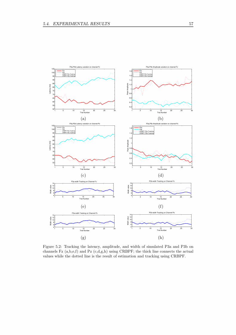
5.4. EXPERIMENTAL RESULTS 57
1 5 10 15 20 25 3050
55
60
65
70
75
80
85
90
95
100
105
Trial Number
La
ten
cy [
ms]
P3a,P3b Latency variation on channel Fz
P3a
P3b
CRBPF P3a Tracking
CRBPF P3b Tracking
1 5 10 15 20 25 30
0.2
0.4
0.6
0.8
1
1.2
1.4
1.6
1.8
Trial Number
Pe
ak A
mp
litu
de
P3a,P3b Amplitude variation on channel Fz
P3a
P3b
CRBPF P3a Tracking
CRBPF P3b Tracking
(a) (b)
1 5 10 15 20 25 30
55
60
65
70
75
80
85
90
95
100
105
Trial Number
La
ten
cy [
ms]
P3a,P3b Latency variation on channel Pz
P3a
P3b
CRBPF P3a Tracking
CRBPF P3b Tracking
1 5 10 15 20 25 30
0.2
0.4
0.6
0.8
1
1.2
1.4
1.6
Trial Number
Pe
ak A
mp
litu
de
P3a,P3b Amplitude variation on channel Pz
P3a
P3b
CRBPF P3a Tracking
CRBPF P3b Tracking
(c) (d)
1 5 10 15 20 25 304
6
8
10
12
14
Trial Number
Wid
th v
alu
e
P3a width Tracking on Channel Fz
1 5 10 15 20 25 304
6
8
10
12
14
Trial Number
Wid
th v
alu
e
P3b width Tracking on Channel Fz
(e) (f)
1 5 10 15 20 25 304
6
8
10
12
14
Trial Number
Wid
th v
alu
e
P3a width Tracking on Channel Pz
1 5 10 15 20 25 304
6
8
10
12
14
Trial Number
Wid
th v
alu
e
P3b width Tracking on Channel Pz
(g) (h)
Figure 5.2: Tracking the latency, amplitude, and width of simulated P3a and P3b onchannels Fz (a,b,e,f) and Pz (c,d,g,h) using CRBPF; the thick line connects the actualvalues while the dotted line is the result of estimation and tracking using CRBPF.

5.4. EXPERIMENTAL RESULTS 58
particles marked invalid in each trial. The average computational time for exe-
cution of CRBPF in each trial was about 0.7533 of a second (using Pentium(R)
4 CPU 3.00GHz, 3.00 GB of RAM).
The available SNR is measured in dB unit and defined as:
SNR = 10log10(Psignal
Pnoise) (5.12)
The MSE is defined as:
MSE =1
N
N∑
i=1
(zact(i) − zest(i))2 (5.13)
where zact is the original clean observation, zest is the estimated observation,
and N is the number of time samples. It can be seen from Fig. 5.2(e,g) that the
same width is estimated for P3a at Fz and Pz channels. The same width is also
estimated for P3b at Fz and Pz channels (see Fig. 5.2(f,h)). In the first 10 trials,
since the filter has not converged, the latency and amplitude estimations, as in
Fig. 5.2(a,c,b,d) are not accurate enough. In the subsequent trials the CRBPF
converges and has clearly better estimation.
In the last few trials, however, some deviations in the estimation of ERP
subcomponent parameters can be seen. This is due to the fact that in each trial,
the amplitudes, latencies, and widths, as the states, are generated randomly,
and the SNR values are also small. In Fig. 5.3 the calculated MSE and SNR
of each trial are shown for Fz and Pz channels in the top and bottom rows. It
can be seen from Fig. 5.3(d) that SNR value for the signal in channel Pz is
close to 1 and decreases slightly in the later trials. Therefore, in some trials the
exact track is lost because of low SNR. Similar to the first trials, however, as the
iterations continue, the estimated values are expected to converge to the actual
values again.
It can be seen from Fig. 5.3 that the SNR values are moderate in most of
realistic situations. On the other hand, the calculated MSE is very low and the
tracking is towards the actual values. Although the exact track may be lost in
some trials due to the low SNR or sudden change in one of the variables, we
still have a very good estimation for the parameters. The important issue is the
trend for variations of the parameters which is mostly preserved even after de-
viation from the actual values. The trend of variations is especially useful when
the SNR is negative in which almost all methods fail. However the advantage
of tracking across trials is that instead of direct estimation of the parameters,
the information from previous trials are taken into account. Therefore, using

5.4. EXPERIMENTAL RESULTS 59
1 5 10 15 20 25 300
0.01
0.02
0.03
0.04
0.05
0.06
0.07
0.08
Trial Number
Mean S
quare
Err
or
Channel Fz
1 5 10 15 20 25 300
1
2
3
4
5
Trial Number
SN
R [dB
]
Fz Channel
(a) (b)
1 5 10 15 20 25 300
1
2
3
4
5
6
7
8x 10
−3
Trial Number
Mean S
quare
Err
or
Channel Pz
1 5 10 15 20 25 300
0.5
1
1.5
2
2.5
3
3.5
Trial Number
SN
R [dB
]
Channel Pz
(c) (d)
Figure 5.3: The corresponding MSE, (a) and (c), and SNR, (b) and (d), calculated indifferent trials for the simulated data for Fz (top) and Pz (bottom) channels.
a tracking based system such as CRBPF, the trends for variations of the pa-
rameters will reveal important information such as increase or decrease of the
parameter values across trials. In order to see how the CRBPF works in very
low SNRs, in the second simulated signals negative SNRs are also considered.
Effect of Mismatch
In the first set of simulated signals the generated P3a and P3b were exact Gaus-
sian waveforms. However in the real case P3a and P3b may not be exactly
Gaussians. Therefore, in the second set of simulated signals we modelled the
P3a and P3b as another waveform to better generalize application of the method.
Gamma waveform defined as:
r(t) = ctk−1exp(− t
θ) (5.14)
where k > 0 is a shape parameter, θ > 0 is a scale parameter, and c is a
normalizing constant, is used as an appropriate alternative. The Gamma waves
for P3a and P3b are shown in Fig. 5.4. In this figure k = 3 and θ = 17 are used
for generating both Gamma waves. In this experiment 30 trials are generated.
The noise variance for the latency is 3 and for the amplitude is 0.1.

5.4. EXPERIMENTAL RESULTS 60
250 300 350 4000
0.2
0.4
0.6
0.8
1
1.2
Time[ms]
Am
plit
ud
e
Gaussians
Gamma
Figure 5.4: Two Gamma waves are used for modelling P3a and P3b. Different Gaussiansapproximating Gamma waves are also shown.
In each trial, the clean observations which are sum of two Gamma waves as
shown in Fig. 5.4 are added with a random noise of variance 0.3. The shape
of Gamma waveforms remains the same across all the trials. The aim of this
experiment is to verify whether the CRBPF is able to work in the case of having
other shapes rather than Gaussians for the original P3a and P3b signals. The
experiment is repeated two times and the results of tracking the latency and
amplitude variations of P3a and P3b at Fz and Pz channels are shown in Fig.
5.5 and Fig. 5.6. Also, in these figures the MSE and SNR are shown in each
trial for each channel.
In Fig. 5.5(a) and Fig. 5.5(e) latency variations of P300 subcomponents
(P3a and P3b) at Fz and Pz channels are shown respectively. In the last trials
a bias in latency estimation for P3b can be seen. However, from Fig. 5.5(d) and
Fig. 5.5(h), it can be seen that the SNR values in the last trials are very low. In
Fig. 5.5(b) and Fig. 5.5(f) the amplitude variations for the P300 subcomponents
(P3a and P3b) at Fz and Pz channels are shown respectively. From these figures
the total variability of the amplitudes are preserved while there are some error
in estimation.
In addition, since the estimated P300 signal is based on the Gaussian as-
sumption of the P3a and P3b while the actual P3a and P3b are Gamma waves,
it can be seen that the calculated MSE in each trial for Fz and Pz channels
shown in Fig. 5.5(c) and Fig. 5.5(g) are high. The estimated width for P3a and
P3b had some fluctuations at the initial trials but they remained constant over
time. The estimated width corresponds to the width of Gaussian waveform. This
however, may not refer to the width of a Gamma wave. The important point
is that we kept the width of Gamma waves the same across different trials and
the estimated width remained constant after the first few trials. The estimated

5.4. EXPERIMENTAL RESULTS 61
1 5 10 15 20 25 3050
60
70
80
90
Trial Number
Late
ncy [m
s]
1 5 10 15 20 25 30
0.5
1
1.5
Trial Number
Peak A
mplit
ude
(a) (b)
1 5 10 15 20 25 300
0.05
0.1
Trial Number
Mean S
quare
Err
or
1 5 10 15 20 25 30−6
−4
−2
0
2
4
Trial Number
SN
R [
dB
]
(c) (d)
1 5 10 15 20 25 3050
60
70
80
90
Trial Number
Late
ncy [m
s]
1 5 10 15 20 25 300
0.5
1
1.5
Trial Number
Peak A
mplit
ude
(e) (f)
1 5 10 15 20 25 300
0.05
0.1
Trial Number
Mean S
quare
Err
or
1 5 10 15 20 25 30−6
−4
−2
0
2
4
Trial Number
SN
R [
dB
]
(g) (h)
Figure 5.5: The dotted lines are the results of tracking using CRBPF, (a) latencyvariations of P3a (red line) and P3b (Blue line) on channel Fz, (b) amplitude variationsof P3a (red line) and P3b (Blue line) on channel Fz, (c) MSE obtained at each trial forchannel Fz, (d) calculated SNR at each trial for channel Fz, (e) latency variations ofP3a (red line) and P3b (Blue line) on channel Pz, (f) amplitude variations of P3a (redline) and P3b (Blue line) on channel Pz, (g) MSE obtained at each trial for channel Pz,and (h) calculated SNR at each trial for channel Pz.

5.4. EXPERIMENTAL RESULTS 62
width for each of Gamma-based P3a and P3b relates to the width of a Gaussian
that can best approximate them.
Therefore, based on the results of this experiment, in the case of Gamma
waveforms for P3a and P3b and despite very low SNRs, the CRPBF can still
track inter-trial variabilities of the P3a and P3b parameters with very good
approximations. This conclusion has been verified by repetition of the experi-
ment as shown in Fig. 5.6. In this figure the results of tracking P3a and P3b
amplitudes and latencies at Fz and Pz channels are shown (Fig. 5.6(a,b,e,f)).
The SNR and MSE in each trial for Fz and Pz channels are also shown (Fig.
5.6(c,d,g,h)). In this figure, the SNR value is very low in most of the trials
and the actual generated signals for P3a and P3b are Gamma waveforms. The
CRBPF nevertheless, is still able to track the inter-trial variabilities of the P3a
and P3b.
5.4.2 Real Data
The description of the real data is explained in Section 4.5.2. EEG data of
one of the subjects was selected. Using interpolation the sampling frequency
was increased to 1000Hz in order to increase the temporal resolution. So, for
example, a shift of less than 0.01 second in latency can be tracked. Previously,
this data set was being used for P300 detection by the averaging method [92].
The CRBPF was applied to Fz and Pz channels considering 50 trials from
the first and fourth half an hour. In the first half an hour the subject was not
under fatigue while in the fourth half an hour the subject was under fatigue. In
both cases, before and during fatigue, the averaged ERP of 20 trials was used
to initialize the particles of the CRBPF.
The results of tracking P3a and P3b variability are shown in Fig. 5.7. This
figure illustrates the variability of P3a and P3a amplitudes (Fig. 5.7(c,d,g,h)),
latencies (Fig. 5.7(a,b,e,f)), and widths (Fig. 5.7(i,j,k,l)) before and during
fatigue state. Based on the results it is possible to draw some conclusions about
the effect of mental fatigue on P300. Generally in the previous researches on
mental fatigue [70, 71, 72, 73, 74], the decrease in the overall P300 amplitude
and increase in its latency have been reported. But, using our method we could
separate P300 into its constituent subcomponents and evaluate the effect on each
subcomponent separately. Based on the results it is concluded that the latencies
of both P3a and P3b increase with time on task interval. During the fatigue
state the increase of the latency of P3a is slightly more than that for the P3b.
Indeed, the amplitude of P3a decreases with fatigue more than that of the P3b.
The width of P3b remains approximately constant in the fatigue state while the
width of P3a decreases.

5.4. EXPERIMENTAL RESULTS 63
1 5 10 15 20 25 30
50
60
70
80
90
100
Trial Number
Late
ncy [m
s]
1 5 10 15 20 25 300
0.5
1
1.5
Trial Number
Peak A
mplit
ude
(a) (b)
1 5 10 15 20 25 300
0.02
0.04
0.06
0.08
0.1
Trial Number
Mean S
quare
Err
or
1 5 10 15 20 25 30−6
−4
−2
0
2
Trial Number
SN
R [
dB
]
(c) (d)
1 5 10 15 20 25 30
50
60
70
80
90
100
Trial Number
Late
ncy [m
s]
1 5 10 15 20 25 300
0.5
1
1.5
Trial Number
Peak A
mplit
ude
(e) (f)
1 5 10 15 20 25 300
0.02
0.04
0.06
0.08
Trial Number
Mean S
quare
Err
or
1 5 10 15 20 25 30−6
−4
−2
0
2
Trial Number
SN
R [
dB
]
(g) (h)
Figure 5.6: The dotted lines are the results of tracking using CRBPF, (a) latencyvariations of P3a (red line) and P3b (Blue line) on channel Fz, (b) amplitude variationsof P3a (red line) and P3b (Blue line) on channel Fz, (c) MSE obtained at each trial forchannel Fz, (d) calculated SNR at each trial for channel Fz, (e) latency variations ofP3a (red line) and P3b (Blue line) on channel Pz, (f) amplitude variations of P3a (redline) and P3b (Blue line) on channel Pz, (g) MSE obtained at each trial for channel Pz,and (h) calculated SNR at each trial for channel Pz.
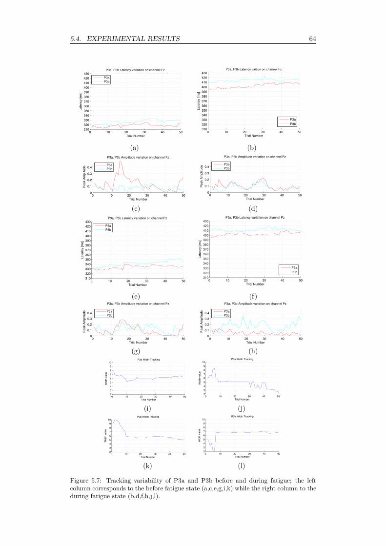
5.4. EXPERIMENTAL RESULTS 64
0 10 20 30 40 50310
320
330
340
350
360
370
380
390
400
410
420
430
Trial Number
Late
ncy [m
s]
P3a, P3b Latency variation on channel Fz
P3a
P3b
0 10 20 30 40 50310
320
330
340
350
360
370
380
390
400
410
420
430
Trial Number
Late
ncy [m
s]
P3a, P3b Latency vaition on channel Fz
P3a
P3b
(a) (b)
0 10 20 30 40 500
0.1
0.2
0.3
0.4
Trial Number
Peak A
mplit
ude
P3a, P3b Amplitude variation on channel Fz
P3a
P3b
0 10 20 30 40 500
0.1
0.2
0.3
0.4
Trial NumberP
eak A
mplit
ude
P3a, P3b Amplitude variation on channel Fz
P3a
P3b
(c) (d)
0 10 20 30 40 50310
320
330
340
350
360
370
380
390
400
410
420
430
Trial Number
Late
ncy [m
s]
P3a, P3b Latency variation on channel Pz
P3a
P3b
0 10 20 30 40 50310
320
330
340
350
360
370
380
390
400
410
420
430
Trial Number
Late
ncy [m
s]
P3a, P3b Latency variation on channel Pz
P3a
P3b
(e) (f)
0 10 20 30 40 500
0.1
0.2
0.3
0.4
Trial Number
Peak A
mplit
ude
P3a, P3b Amplitude variation on channel Pz
P3a
P3b
0 10 20 30 40 500
0.1
0.2
0.3
0.4
Trial Number
Peak A
mplit
ude
P3a, P3b Amplitude variation on channel Pz
P3a
P3b
(g) (h)
0 10 20 30 40 502
3
4
5
6
7
8
9
10
Trial Number
Wid
th v
alu
e
P3a Width Tracking
0 10 20 30 40 502
3
4
5
6
7
8
9
10
Trial Number
Wid
th v
alu
e
P3a Width Tracking
(i) (j)
0 10 20 30 40 502
3
4
5
6
7
8
9
10
Trial Number
Wid
th v
alu
e
P3b Width Tracking
0 10 20 30 40 502
3
4
5
6
7
8
9
10
Trial Number
Wid
th v
alu
e
P3b Width Tracking
(k) (l)
Figure 5.7: Tracking variability of P3a and P3b before and during fatigue; the leftcolumn corresponds to the before fatigue state (a,c,e,g,i,k) while the right column to theduring fatigue state (b,d,f,h,j,l).

5.5. CONCLUSIONS 65
The P3a amplitude seems to become smaller with time on the task, while
that of the P3b seems to increase somewhat. During the first half an hour a
clear difference between the P3a and P3b locations over scalp is observed. P3a
is more prominent at Fz as expected. During the last half an hour the P3a
became very small at Pz while the P3b was prominent at this position. P3a is
related to novelty. It is possible however that the decrease in the P3a amplitude
with time on the task is related to practice on or habituation to the task.
Therefore, mental fatigue can be related to increase in the P3a and P3b
latencies, and decrease in the P3a amplitude and width. Using the results of
this research the amplitude and width of P3a and latencies of P3a and P3b,
obtained by applying CRBPF, can be considered as useful features for detec-
tion of fatigue state. However, these features are not enough for distinguishing
between the different mental states and alarming the fatigue state. In future
studies a comprehensive analysis of mental fatigue can be performed by combi-
nation of these extracted features along with other useful features, from different
ERP components and subcomponents and the background EEG, and then giving
them as an input to a classifier in order to classify different mental states. In
addition, it is possible to use all the features obtained by applying the proposed
CRBPF in this chapter including latency, amplitude, and width of both P3a and
P3b. Then, an appropriate feature selection method can be used to mark and
remove the useless features.
5.5 Conclusions
In this chapter a new method is proposed to separate and track variability of
P300 subcomponents in different single trials. The method has been applied to
investigate mental fatigue. The coupled PF proposed in this chapter uses the
concept of RBPF, combines two RBPFs, and imposes some constraints on the
state variables to have a more reliable estimation and to use the required number
of particles effectively. The particle initialization with the help of averaged ERP
is useful to move the particles towards the right part of the posterior density.
Therefore, the algorithm is capable of estimating P300 component and its sub-
components P3a and P3b in single trials. Here, for the first time, all variations
of the P300 subcomponents (P3a and P3b) including latency, amplitude, and
width, have been considered from single trials and applied to the mental fatigue.
It is known that P3a is an attention related subcomponent and P3b is a memory
related subcomponent [22]. Therefore, during the fatigue state the attention to
the stimuli decreases more than the memory engagement with the stimuli.

5.5. CONCLUSIONS 66
This single trial estimation can reveal important information about the vari-
ability of P300 subcomponents which cannot be achieved by detection of aver-
aged P300 as in previous researches whereby the variability of the subcomponents
is ignored. Therefore, this new single trial estimation of ERP subcomponents
has shown to be favourably effective in mental fatigue analysis. In addition, the
designed coupled RBPF is able to synchronously and simultaneously character-
ize two dependent systems and therefore can be applicable for monitoring many
natural systems.
Although the proposed method is based on fitting Gaussians to ERP signals
and using application specific constraints, the risk of generating responses that
do not exist in the data is avoided by particle initialization using the averaged
ERP and especially by coupling the two measurement channels. The coupling
is possible since the P3a and P3b are expected to be statistically dependent
(e.g. temporal order, correlated amplitudes, etc). Using prior knowledge about
other ERP subcomponents, it is possible to use the method with appropriate
constraints. In addition, the method can be combined with beamforming algo-
rithms to introduce a spatio-temporal approach for analysis of ERP subcompo-
nents. The results achieved in this work are inline with clinical expectations.
They also verify previous reported outcomes by [70, 71, 72, 73, 74]. However,
the method has the ability to give more insight about the relative changes of
P300 subcomponents. The method presented in this chapter is useful for tem-
poral estimation of ERP subcomponents. In the next chapter, a new single trial
estimation method is proposed for spatio-temporal estimation of ERP subcom-
ponents.

Chapter 6
Spatio-temporal Filtering
Method for Single Trial
Estimation of Correlated ERP
Subcomponents
6.1 Introduction
In the previous chapter a method based on PF was proposed for tracking variabil-
ity of ERP subcomponents from two channels. The method only considers the
temporal variations of the ERP subcomponents across different trials whereas the
spatial relationships are ignored. Therefore, a new method for spatio-temporal
estimation of ERP subcomponents is demanded.
In this chapter a novel spatio-temporal filtering method is proposed for sin-
gle trial estimation of ERP subcomponents which can be mutually correlated.
The method can be specifically used for spatio-temporal estimation of P300 sub-
components (e.g. P3a and P3b). These subcomponents can be generated in
an oddball paradigm considering the target stimuli. It is hypothesized that the
discrimination between target and standard stimuli initiates the frontal lobe ac-
tivity that engages the attention focus demanded by the task performance [100].
P3a is supposed to be related to the neural changes in the anterior cingulate when
the incoming stimuli replace the contents of working memory [101]. P3b is then
generated from memory storage operations that are initiated in the hippocampal
formation in which the update output is transmitted to the parietal cortex [102].
Therefore, the P3a is generated when a demanding stimuli commands frontal
lobe attention and subsequently P3b is generated when the required attention
67

6.1. INTRODUCTION 68
resources are allocated for memory updating in association cortex. Based on
this model, the P300 component generation is due to the interaction between
frontal lobe and hippocampal/temporal-parietal function. Although the exact
neural origins of P3a and P3b are distinct, the generation of these subcompo-
nents involve interactions between them and as the result engages overlapping
neural activations [100]. Based on this, these subcomponents are correlated.
Throughout this study, the correlation of ERPs in temporal or spatial domain is
considered as the overlap in time or space domain which can be seen from statis-
tical point of view of the scalp projections and time domain series of the ERPs.
However, in general the overlap is the sign of neural generation/interactions of
the ERP components/subcomponents.
Recently a method for spatio-temporal estimation of ERP components has
been developed [103]. The advantage of this method is that instead of modelling
the whole ERP component, it models its descriptors (amplitude and latency)
based on the spatial diversity of multi-channel recordings and a user defined
template. This method has shown to be effective in ERP component estimation
even in negative SNRs. However, although this method can be used for single
trial estimation of ERP components, it is not suitable for estimation of the ERP
subcomponents particularly when they overlap in time.
Hence, in the case of having correlated components or subcomponents the
method cannot achieve correct results. Therefore, in this chapter we have signif-
icantly improved the method presented in [103] by developing a spatio-temporal
filtering method for single trial estimation of correlated ERP subcomponents. In
[82] a spatial notch filter is used to localize the ERP subcomponents in the brain.
In this approach the correlation between the desired component and the back-
ground EEG has been considered. In our proposed method for spatio-temporal
estimation of the ERP subcomponent descriptors two cost functions are defined
first. Following that, the latencies, amplitudes, and scalp projections of both
subcomponents are estimated. Each cost function can deflate one of the corre-
lated subcomponents and estimate the other one. In general, the subcomponents
are considered to be temporally/spatially correlated.
It is possible to generalize the method to be considered for the cases where
there are more than two subcomponents. In this chapter in Section 6.2, it is
shown mathematically that the method presented in [103] for estimation of the
ERP components is not suitable for ERP subcomponent estimation because of
temporal correlation between the subcomponents. The new method proposed
here however, can result in a very good estimation of ERP subcomponent de-
scriptors.

6.2. LINEAR GENERATIVE EEG MODEL 69
Therefore, unlike the previous works in ERP estimation [82, 103], the pro-
posed method is able to estimate the subcomponents such as P3a and P3b. The
method is applied to both simulated and real data and has shown to perform
very well even in low SNRs. The method has been compared with the spatial
PCA and its superiority confirmed by using simulated signals. In addition, the
two methods were compared in different spatial correlations. Finally it has been
compared with temporal PCA for different temporal correlations. The approach
can be useful in mental fatigue analysis where the relative variability of P300
subcomponents is the key factor in detecting the level of fatigue.
The remainder of this chapter is structured as follows. In Section 6.2 lin-
ear generative EEG model is described. Then, in Section 6.3, the new spatio-
temporal filtering method is proposed. In Section 6.4 the results of applying the
spatio-temporal filtering to simulated data following by a comparison study are
provided. The results of applying the method to the real data are provided in
Section 6.5. Finally, Section 6.6 concludes the chapter.
6.2 Linear Generative EEG Model
In this section a composite EEG model including two (generally correlated)
subcomponents is provided. For this we start with writing the linear generative
EEG model in matrix form as:
X = a s +
N∑
i=1
bini (6.1)
where X is a D × T matrix which represents the single trial EEG data of D
channels and T samples, s is a 1 × T vector that can represent the time course
of ERP component, ni denotes the 1×T noise in general, and N is the number
of noise components. The vectors aT and bTi are of dimension 1×D and can be
considered as the projections of the corresponding source and background EEG
plus noise to the electrodes respectively, X can also be modelled in terms of its
constituent normalized components as:
X = σs0a0s0 +N∑
i=1
σib0in0i (6.2)
where a0, s0, and n0i are the normalized versions of their counterparts in (6.1).
The scalars σs0 and σi are the overall contributions of the sources to the multi-
channel EEG data. It is expected that for a stable normalized scalp projection,
6.2. LINEAR GENERATIVE EEG MODEL 70
a0 is fixed for all the trials and the amplitude σs0 changes across trials. Now, con-
sider a new equivalent formulation with respect to ERP subcomponents which
are potentially correlated (at this stage it is assumed that there are two over-
lapped subcomponents as the case for P3a and P3b):
X = σ1a1s1 + σ2a2s2 +
N∑
i=1
σib0in0i (6.3)
where σ1, a1, and s1 are the amplitude, scalp projection, and time course of
the first ERP subcomponent, and σ2, a2, and s2 are those of the second ERP
subcomponent of the combined component described by σs0, a0, s0 in equation
(6.2). Suppose that we have an estimation of the first subcomponent that is nor-
malized as y1. If we post-multiply its transpose to both sides of equation (6.3),
the following relation will be obtained (the cross term n0i.yT1 nearly vanishes be-
cause it is assumed that the noise including the background EEG is uncorrelated
with the ERP subcomponents):
X.yT1 = σ1a1s1y
T1 + σ2a2s2y
T1 (6.4)
If we assume that the normalized estimated subcomponent y1 is exactly the same
as the first subcomponent, the first term will be equal to σ1a1 due to the normal-
ization operation, i.e. s1.yT
1 is equal to 1. The main concern is with the second
term in which s2.yT
1 becomes a scaling factor due to the existence of temporal
correlation between the subcomponents. If s2.yT
1 were zero (having no temporal
correlation), X.yT
1 could result in an estimation of a1. Therefore, multiplication
of one of the estimated subcomponents by X is not useful for estimation of its
corresponding scalp projection due to the nonzero nature of the second term in
equation (6.4) in the case that the subcomponents are temporally correlated.
The above approach has been proposed and used in [103] in order to have an
initial estimation of the scalp projection a of the ERP component which is un-
correlated with the noise. But we showed that in the case of having temporally
correlated ERP subcomponents the method is not able to estimate the scalp
projections of the subcomponents. Hence, it is necessary to extend the method
to work for estimation of the correlated ERP subcomponents. In the next sec-
tion, the proposed spatio-temporal filtering method for solving this problem is
explained.

6.3. SPATIO-TEMPORAL FILTERING METHOD 71
6.3 Spatio-temporal Filtering Method
The proposed spatio-temporal filtering method for estimation of correlated ERP
subcomponents suppresses one subcomponent in spatial domain while detecting
the other one in temporal domain. Now, consider the following constrained
problem:
min ||wTX− r1||22 subject to wTa2 = 0 (6.5)
where both wT and aT2 are 1×D vectors, r1 is a 1×T vector, D is the number
of channels, and T is the number of time samples. The constrained problem can
be converted to an unconstrained problem using Lagrange multipliers leading to
the following cost function:
F = ||wTX− r1||22 + wTa2q (6.6)
where q is the Lagrange multiplier. The gradient of F with respect to wT is:
∂F
∂wT=
∂
∂wTr1r
T1 − 2r1X
Tw + wTXXT w + wTa2q
= −2r1XT + 2wTXXT + qaT
2
(6.7)
By setting the above equation to zero and solving it for wT :
wT = 0.5(2r1XT − qaT
2 )C−1x (6.8)
where Cx = XXT . Since we are not sure if Cx is full rank, we used pseudo-
inverse for C−1x . If (6.8) is substituted into the constraint in (6.5), we obtain:
wTa2 = 0.5(2r1XT − qaT
2 )C−1x a2 = 0; (6.9)
This is solved for q which results in:
q =2r1X
TC−1x a2
aT2 C−1
x a2
(6.10)
Now, consider the main cost function in equation (6.5):
G = ||wT X− r1||22 (6.11)
By setting G to zero and solving it for w, the optimum solution given by wTopt
to extract r1 is given by:
wTopt = r1X
TC−1x (6.12)

6.3. SPATIO-TEMPORAL FILTERING METHOD 72
By pre-multiplying wTopt to both sides of equation (6.3), it can be seen that in
order to have an estimation of s1, in the case of having an appropriate reference
signal for s1 i.e. r1, wTopta1 will be 1/σ1 and wT
opta2 will be zero. Therefore, wTopt
should be orthogonal to a2. If a1 and a2 are orthogonal, then, wTopt can be in
the direction of a1 vector. But this does not necessarily mean that a1 and a2
should be orthogonal. Some simulations showed that even when a1 and a2 are
not orthogonal, wTopt is found in which wT
opta1 is 1/σ1 and wTopta2 is very close
to zero.
The only constraint is that a1 and a2 should not be exactly in the same
direction. This is true for the case of having different ERP subcomponents.
This is because the subcomponents originate from distinct regions of the brain
and therefore, they are spatially disjoint. The scalp projections can also be
described using a forward matrix. This matrix models the mixing process of
the sources at the electrodes. When two sources are from different parts of the
brain, their forward projection vectors and as the result, their scalp projections
are not the same.
Therefore, it is concluded that in the case of having an exact reference for
s1, wTopta1 = 1/σ1 and wT
opta2 = 0. Substituting wTopt from equation (6.12) into
wTopta2 = 0, the following equation will be obtained:
r1XTC−1
x a2 = 0 (6.13)
Equation (6.13) is equal to the numerator of equation (6.10) and therefore, the
Lagrange multiplier will be zero. This is obvious because this makes the cost
functions F and G equal. In other words, when it is reasonable to have wTopta2 =
0 there is no need to add the constraint wTa2 = 0 because as explained, this
holds implicitly.
Since it is shown that having wTa2 = 0 as the constraint in (6.5) is not
helpful, we define a new constrained problem which is similar to (6.5) but with
an alternative constraint. To do that, first a2 in the constraint term in (6.5) is
replaced with a2. Later a suitable choice for a2 is made and it is shown that
solving the new constrained problem leads to the estimation of scalp projection
for one of the correlated subcomponents. Therefore, in a similar manner, the
new constrained problem is defined as:
min ||wTX− r1||22 subject to wT a2 = 0 (6.14)
After converting the constrained problem into an unconstrained problem us-
ing Lagrange multiplier, the new cost function is obtained as:

6.3. SPATIO-TEMPORAL FILTERING METHOD 73
F = ||wTX− r1||22 + wT a2q (6.15)
Following equations (6.9) and (6.10) the following solution for the Lagrange
multiplier is achieved:
q =2r1X
TC−1x a2
aT2 C−1
x a2
(6.16)
With the help of equations (6.8) and (6.16) wT is calculated as follows:
wT = r1XTC−1
x − r1XTC−1
x a2
aT2 C−1
x a2
aT2 C−1
x (6.17)
or
w = C−1x XrT
1 − r1XTC−1
x a2
aT2 C−1
x a2
C−1x a2 (6.18)
We pre-multiply both sides of the above equation by XT to obtain the following
equation:
XTw = XTC−1x XrT
1 − r1XTC−1
x a2
aT2 C−1
x a2
XTC−1x a2 (6.19)
A suitable choice is made for a1 and a2 as:
a1 = XrT1
a2 = XrT2
(6.20)
Therefore, it is simple to derive the following equations using equations (6.3)
and (6.20):
a1 = σ1a1s1rT1 + σ2a2s2r
T1
a2 = σ1a1s1rT2 + σ2a2s2r
T2
a1 = σ1a1s1rT1 +
(a2 − σ1a1s1rT2 )
s2rT2
s2rT1
a1 = σ1a1s1rT1 + a2
s2rT1
s2rT2
− σ1a1s1r
T2 (s2r
T1 )
s2rT2
(6.21)
From the above equations, it can be seen that a1 and a2 are linear combinations
of the scaled a1 and a2. Having appropriate reference signals, when the correla-
tion between the subcomponents decreases, a1 tends towards σ1a1 and a2 tends
towards σ2a2.
In fact, even if by solving equation (6.5) we are able to estimate the scalp
projection for one subcomponent, having only the mixture matrix X, we do not

6.3. SPATIO-TEMPORAL FILTERING METHOD 74
have access to a1 or a2 (unless there is no correlation between the subcompo-
nents) in order to solve the constrained problem in (6.5). However, by using
the reference signals r1 and r2, as it is shown in (6.20) and (6.21), we can have
access to the linear combinations of the scaled scalp projections of both subcom-
ponents (a1,a2). Then, we can use any of the linear combinations and solve the
constrained problem in (6.14). In the following equations, we show that having
a2 as defined in (6.20) by solving the constrained problem in (6.14) the scalp
projection for the first subcomponent (a1) is estimated. The same procedure can
be implemented in order to find the scalp projection for the second subcompo-
nent (a2). By replacing a1 from equation (6.21) in equation (6.19), the following
equations can be derived:
XTw = XTC−1x XrT
1 − aT1 C−1
x a2
aT2 C−1
x a2
XTC−1x a2
= XTC−1x XrT
1
−[σ1s1r
T1 aT
1 +s2r
T1
s2rT2aT
2 − σ1s1r
T2 (s2rT
1 )
s2rT2
aT1 ]C−1
x a2
aT2 C−1
x a2
XTC−1x a2
(6.22)
At this stage it is desired to show that aT1 C−1
x a2 = 0. Consider equation (6.13)
and use it with swapped indices as:
r2XTC−1
x a1 = 0
aT2 C−1
x a1 = 0
aT1 C−1
x a2 = 0
(6.23)
These can be used to simplify equation (6.22) to:
XTw = XTC−1x XrT
1 −[s2r
T1
s2rT2aT
2 ]C−1x a2
aT2 C−1
x a2
XTC−1x a2
= XTC−1x XrT
1 − [s2r
T1
s2rT2
]XT C−1x a2
= XTC−1x [σ1a1s1r
T1 + σ2a2s2r
T1 ]
− XTC−1x [
s2rT1
s2rT2
][σ1a1s1rT2 + σ2a2s2r
T2 ]
= XTC−1x [σ1a1s1r
T1 + σ2a2s2r
T1 ]
− XTC−1x [
s2rT1
s2rT2
σ1a1s1rT2 + σ2a2s2r
T1 ]
(6.24)

6.3. SPATIO-TEMPORAL FILTERING METHOD 75
Then, XTw can be simplified more into:
XT w = XTC−1x [σ1a1s1r
T1 ] − XTC−1
x [s2r
T1
s2rT2
σ1a1s1rT2 ]
= XTC−1x σ1a1[s1r
T1 − s2r
T1
s2rT2
(s1rT2 )]
(6.25)
By pre-multiplying equation (6.25) by X,
XXTw = XXT C−1x σ1a1[s1r
T1 − s2r
T1
s2rT2
(s1rT2 )] (6.26)
Since Cx = XXT and XXTC−1x = I, the following equation is derived:
XXTw = σ1a1[s1rT1 − s2r
T1
s2rT2
(s1rT2 )] (6.27)
If XXTw is normalized to unit variance, a1 will be obtained. Therefore, following
(6.20) by using a2 = XrT2 , minimizing equation (6.15), solving it for w, and pre-
multiplying the resulted w, first by XT and then by X, we can have an estimate
of a1. This is the scalp projection of the first subcomponent whose corresponding
temporal reference signal is given by r1.
Therefore, equation (6.15) is shown to be useful in estimation of the scalp
projection of one of the correlated subcomponents. Considering equation (6.15)
and the results given by equation (6.27), the procedure for estimating the scalp
projection of the first subcomponent is illustrated in Algorithm 6.1.
Algorithm 6.1: ESP1 Estimation of the scalp projection
for the first subcomponent
a1 = ESP1 (X,r1,r2)
-Set C−1x = (XXT )−1
-Set a2 = XrT2 (see eq. 6.20)
-Find q = 2(r1XTC−1
x a2)/(aT2 C−1
x a2) (see eq. 6.16)
-Find w = C−1x XrT
1 − 0.5qC−1x a2 (see eq. 6.18)
-Estimate a1 = (XXT w)/norm(XXTw) see (eq. 6.27)
Return a1
Similarly, to enable estimation of the scalp projection for the second subcom-
ponent, equation (6.15) can be replaced by the following equation:
F = ||wTX− r2||22 + wT a1q (6.28)
Using the above equation, the same procedure can be followed in order to find the

6.3. SPATIO-TEMPORAL FILTERING METHOD 76
scalp projection of the second subcomponent. The Pseudo-code for estimating
the scalp projection of the second subcomponent is illustrated in Algorithm 6.2.
Algorithm 6.2: ESP2 Estimation of the scalp projection
for the second subcomponent
a2 = ESP2 (X,r1,r2)
-Set C−1x = (XXT )−1
-Set a1 = XrT1
-Find q = 2(r2XTC−1
x a1)/(aT1 C−1
x a1)
-Find w = C−1x XrT
2 − 0.5qC−1x a1
-Estimate a2 = (XXT w)/norm(XXTw)
Return a2
Incorporating and estimating the spatial projecting vectors a1 and a2 into
the temporal least square (6.15) and estimation of wT significantly improve the
results and enable separation of temporally or spatially correlated signals such
as P3a and P3b. One achievement which has also been confirmed by simulation
is that in the case of a mismatch between the reference signal and the actual
source the normalized vector of XXTw does not change (or because of different
noise level it changes very slightly). In other words, the estimation of scalp
projection of one of the ERP subcomponents is not exactly dependent on the
shape of the reference signals. These references, although reasonably similar to
the source signals, are not their exact replications. When there is a mismatch
between the actual source and the reference signal, we can still have a very good
approximation of scalp projections of the subcomponents. This is due to the
fact that the mismatch results in the change of the scale ([s1rT1 − s2r
T1
s2rT2(s1r
T2 )])
in equation (6.27) in the estimation. After normalization however, this has no
effect in estimation of the scalp projection.
In other words, the scale contains the dot product of the actual sources and
the reference signals. If the reference is not exactly the same as the source signal,
we have a different scale; however after normalization, the scale will not influence
estimation of the scalp projections. If both reference signals are uncorrelated
(or slightly correlated) with the source the vector XXT w tends to zero vector.
Therefore, we are able to check whether we are dealing with correct references
(or dealing with meaningful ranges of latencies for given references).
Nevertheless, in order to have a temporal estimation for each subcomponent,
we need to solve equation (6.11) to find wTopt given in (6.12) and then pre-multiply
it by X. Therefore, given a reference signal for each subcomponent, wToptX will
be the temporal estimation of that subcomponent.

6.3. SPATIO-TEMPORAL FILTERING METHOD 77
As stated in Chapter 5, Section 5.2, ERP subcomponents are modelled us-
ing parametric functions in many studies (e.g. see [98, 99]). The macroscopic
EEG electrical field is created from spike trains by a non-linear generator with
a second-order linear component with real poles as noted by Freeman [104].
According to this model, the impulse response of the system is a monophasic
waveform with a single mode, where the rising time depends on the relative
magnitude of the two real poles and can therefore vary compared to the falling
time. This means Gamma functions can best represent the brain activations.
Therefore, like the method in [103] we used Gamma wave as an approximation
to ERP subcomponents. Based on the defined algorithm, first, we generate two
references (r1, r2) which represent the first and second subcomponents using
Gamma functions expressed as:
r(t) = ctk−1exp(− t
θ) (6.29)
where k > 0 is a shape parameter, θ > 0 is a scale parameter, and c is a
normalizing constant. The Gamma function can be considered as a monophasic
waveform with its mode at t = (k − 1)θ, (k > 1). The Gamma wave has a short
rise time and a longer tail for small k, and for the large k it is a symmetric
waveform. The Pseudo-code for the new spatio-temporal filtering method is
shown in Algorithm 6.3. This algorithm uses the procedures in EPS1 and EPS2
algorithms. Gamma waves are used for generating the reference signals. Also
in this algorithm several cost functions are defined in order to have reliable
estimations for the subcomponent parameters.
After generating Gamma wave as a reference signal for each ERP subcom-
ponent, we slide each reference in a range of valid latencies to generate more
reference signals for both subcomponents. We represent the peak latency of
the reference as τ . Having generated references, the value of a1 and a2 can be
obtained using equation (6.20). Then, it is possible to solve the unconstrained
problems given in (6.15) and (6.28) considering each reference and ai (i=1,2)
that is obtained by using the reference for another subcomponent. Next, we
estimate w1(τ1) and w2(τ2) using equation (6.18) as shown in EPS1 and EPS2
Algorithms.
Then, considering three cost functions (J1(τ1), J2(τ2), and J(τ1, τ2)), we
choose the reference signals for which the sum of the three cost functions is
minimum. Finally, we are able to estimate a1, a2, σ1, and σ2. Practically, better
results are achieved in estimation of peak latency if we use J(τ1, τ2) cost function.
This cost function is obtained from equations (6.11) and (6.12) by considering
sum of the reference signals and also each reference signal separately. This is

6.4. SIMULATION RESULTS 78
not surprising since for temporal estimation of the subcomponents it is preferred
to use wopt given in equation (6.12) and for the estimation of scalp projection
and the amplitude it is better to use the constrained problem given in (6.14).
Therefore, for estimation of the peak latency we use wopt resulted when using the
reference signals for each subcomponent and considering J(τ1, τ2) cost function.
Algorithm 6.3 New spatio-temporal filtering method
-Generate r1(τ1),r2(τ2) considering reasonable ranges of peak
latencies [τ1 ∈ Ts1, τ2 ∈ Ts2] for the first and second
subcomponents using Gamma waves
-Set a1(τ1) = Xr1(τ1)T and a2(τ2) = Xr2(τ2)
T
-Find w1(τ1) = C−1x Xr1(τ1)
T − r1(τ1)XT C−1x a2(τ2)
aT2 (τ2)C−1
x a2(τ2)C−1
x a2(τ2)
w2(τ2) = C−1x Xr2(τ2)
T − r2(τ2)XTC
−1x a1(τ1)
aT1 (τ1)C−1
x a1(τ1)C−1
x a1(τ1)
-Set J1(τ1) = ||wT1 (τ1)X − r1(τ1)||22 + w1(τ1)
T a2(τ2)q
J2(τ2) = ||wT2 (τ2)X− r2(τ2)||22 + w2(τ2)
T a1(τ1)q
J(τ1, τ2) = ||(r(τ1) + r(τ2))[XT C−1
x X − I]||22+
||r(τ1)[XTC−1x X− I]||22 + ||r(τ2)[XTC−1
x X − I]||22[l1, l2] = argmin
τ1,τ2
(J1(τ1) + J2(τ2) + J(τ1, τ2))
-Estimate a1 = XXT w1(l1)norm(XXT w1(l1))
a2 = XXT w2(l2)norm(XXT w2(l2))
σ1 = 1/[(r1(l1)XTC−1
x )(a1)]
σ2 = 1/[(r2(l2)XTC−1
x )(a2)]
-Find the peak latencies as [τ1, τ2] = argminτ1,τ2
J(τ1, τ2)
6.4 Simulation Results
In this section, the method is applied to simulated data and the corresponding
results are demonstrated. The goal of the simulation study is to evaluate the
ability of the method in estimation of peak latency, amplitude, and scalp pro-
jection of the ERP subcomponents in single trials in different SNR levels. In
addition, the performance of the proposed method and the PCA method have
been compared. In the following, the PCA, spatial PCA, and temporal PCA

6.4. SIMULATION RESULTS 79
methods are briefly described. Then, a comparison study including the simula-
tion results is provided.
6.4.1 PCA, Temporal PCA, Spatial PCA, and Spatio-temporal
PCA
Statistical decomposition of ERPs has been of great interest among ERP re-
searchers over the past several decades. A variety of methods have been pro-
posed in which PCA [105, 106, 107] has been the simplest and most widely used
method. PCA uses eigenvalue decomposition to extract linear combinations of
variables from a data covariance matrix. Therefore, PCA can be performed by
eigenvalue decomposition of a data covariance matrix or by singular value de-
composition (SVD) of a data matrix. In SVD decomposition the data matrix is
usually mean centered for each variable.
The target outputs of a PCA algorithm are the component scores and load-
ings. The component scores are the transformed variable values corresponding
to a particular case in the data while the component loadings are the variance
each original variable would have if the data were projected onto a given PCA
axis. Mathematically, PCA can be considered as an orthogonal linear trans-
formation that transforms the data to a new coordinate system. In the new
coordinate system, the greatest variance by any projection of the data comes to
lie on the first coordinate in which is called the first principal component. Then,
the second greatest variance lie on the second coordinate as the second principal
component, and so on [106]. Suppose the data matrix XT is available; this data
matrix contains n rows, which represent n observations, and m columns which
represent m features. The SVD of X is given by:
X = BΣVT (6.30)
where B is the m × m matrix of the eigenvectors of XXT , Σ is the m × n
rectangular diagonal matrix with nonnegative real numbers on the diagonal,
and matrix V is n × n. When the same number of principal components as
original variables are obtained, then PCA has preserved the dimensionality as:
YT = XT B
= VΣT
(6.31)
In the cases where m < n− 1, V is not uniquely defined whereas Y is uniquely

6.4. SIMULATION RESULTS 80
defined. Each row of YT is a rotation of the corresponding row of XT . This is
due to the fact that by definition of the SVD of a real matrix, B is an orthogonal
matrix. The first column of YT consists of the scores with respect to the first
principal component, while the second column has the scores with respect to the
second principal component, and so on.
In a reduced-dimensionality representation, the data matrix X is projected
down into the reduced space defined by only the first L singular vector:
Y = BTLX
= ΣLVTL
(6.32)
Matrix B of eigenvectors of the observation covariances C = XXT matrix is
equivalent to matrix B of singular vectors of X:
XXT = BΣΣTBT (6.33)
If we consider a set of points in Euclidean space, the first extracted principal
component corresponds to a line that minimizes the square sum of the distances
of the points from the line. This line should pass through the multidimensional
mean. In a similar manner, the second extracted principal component corre-
sponds to a line that has the minimum square sum of the distances of the points
from that line. Before extracting the second principal component, all the cor-
relation with the first principal component should be subtracted out from the
points. The singular values in Σ are the square roots of the eigenvalues of matrix
XXT .
Each eigenvalue is proportional to the portion of the variance (square sum
of distances of the points from their multidimensional mean) that corresponds
to each eigenvector. Therefore, the sum of all the eigenvalues is equal to the
square sum of the distances of the points from their multidimensional mean.
PCA algorithm rotates the set of points around their mean in order to find the
principal components. Using an orthogonal transformation, the most variance
is moved into the first few dimensions. The other components which have small
variances can be removed without loss of information. The mean centering (mean
subtraction) of the data before applying PCA is necessary to ensure that the first
principal component represents the direction of maximum variance. If mean
subtraction is not performed, it is possible that the first principal component is

6.4. SIMULATION RESULTS 81
similar to the mean of the data. The first principal component is obtained as:
b1 = argmax‖b‖=1
Var bTX = argmax‖b‖=1
E(bTX)2 (6.34)
Having the first k− 1 extracted principal components, the kth principal compo-
nent can be obtained by subtracting the first k − 1 principal components from
the data matrix X:
Xk−1 = X −k−1∑
i=1
bibTi X (6.35)
By considering Xk−1 as the new data matrix, the next principal component will
be obtained as:
bk = argmax‖b‖=1
E(bT Xk−1)2 (6.36)
In ERP analysis, PCA has been used mainly for separation of the ERP com-
ponents/subcomponents from the background EEG [108, 109]. However, other
applications of PCA can be in data reduction or filtering. This is because PCA
can be used to simplify the analysis of complex data by compressing the impor-
tant information into small number of components.
Factor rotation
PCA is applied to the ERP data in two steps. The first step is principal com-
ponent extraction as explained above. From now on, for simplicity the principal
components are referred to as the factors. This initial extraction results in an
un-rotated solution [108]. The output of the first step is a factor loading matrix
and a factor score matrix. The factor loading matrix relates to the correlations
between the variables and the factor scores while the factor score matrix rep-
resents the magnitude of the factors for each of the observations. Therefore,
the factor score matrix represents the relationship between the factors and the
observations. Multiplication of factor loading and factor score matrices, will
reproduce the data matrix.
In ERP analysis, by applying PCA it is expected to extract ERP subcom-
ponents or components. However, there is not a one-by-one map between the
extracted principal components (factors) and ERP subcomponents/components.
The PCA generates those factors that account for maximum variance. These fac-
tors may be influenced by more than one ERP component/subcomponent after

6.4. SIMULATION RESULTS 82
the initial extraction in the first step [108]. For example a factor can be a hy-
brid of two ERP components (e.g 90% of the one ERP component and 10% of
another ERP component). Since the final goal in applying PCA is to have fac-
tors, each representing one ERP component/subcomponent, a post-processing
technique should be performed on the extracted factors. The used technique is
factor rotation. Factor rotation is used to restructure the allocation of variables
to those factors which are more likely to present the latent variables (ERP com-
ponents/subcomponents). The most common factor rotation is Varimax [110].
In Varimax, the factors are rotated pairwise iteratively, until the change in
the solution is trivial. The Varimax procedure rotates the two factors such that
the sum of the factor loadings is maximized. Therefore, new factors are generated
that are as close to zero for some variables as possible, while others are as large
as possible. It is expected that these generated factors closely correspond to a
single ERP component/subcomponent. This rotation process can be illustrated
as a scatterplot in which the axes are the factors and each point represents a
single variable. The rotation process rotates the axes of the coordinate system
such that the axes pass through the most concentrated groupings of the points.
In other words, the rotation arranges the factor loadings of each variable to be
as large for one factor and as small for the other factors as possible.
The Varimax rotation is sensitive to the correlations and overlap between
the ERP components/subcomponents. Therefore, it affects the accuracy of the
system [108]. In both steps i.e. the initial extraction and Varimax rotation,
the strict orthogonality is maintained between the factors (so the factors are
assumed to be uncorrelated). Therefore, the correlation between ERP compo-
nents/subcomponents violates the statistical uncorrelatedness assumptions. The
more the ERP components/subcomponents are correlated, the more the solu-
tion will be inaccurate and produce misallocation of variance among the factors.
However, component correlation is effectively addressed using oblique rotations
such as Promax [111]. In Promax rotation, the correlation between the factors
are allowed. Promax performs an initial Varimax rotation, then it relaxes the
orthogonality restrictions which allows the factors to become correlated. Con-
sidering the scatter plot, this is equivalent to the Varimax rotation. However
each axis is rotated separately and therefore, there is no need for the axes to be
perpendicular. Therefore, if ERP components/subcomponents are correlated,
using Promax rotation a more accurate solution will be obtained.
Temporal PCA
In temporal PCA, the data matrix is organized in a way that the variables are

6.4. SIMULATION RESULTS 83
the recorded potential at each time point, and the observations correspond to
different waveforms recorded at each channel [108, 109]. Therefore, the number
of variables is equal to the number of time points, and the number of observa-
tions is equal to the number of channels. After arrangement of the data matrix,
PCA is applied to the data matrix for initial component extraction. Then, a
factor rotation algorithm should be applied to the extracted factors. Previous
results suggest that when using the temporal PCA, it is preferred to use the
Promax rotation as the rotation algorithm [108]. The factor loadings which are
the output of the temporal PCA algorithm correspond to the time course of
each factor while the factor score corresponds to the magnitude of each factor
for different channels.
Since the variables in temporal PCA algorithm are the recorded potentials
at each time point, the output consists of the factors that are temporally uncor-
related. Therefore, if in an ERP dataset, the ERP components/subcomponents
are highly correlated in temporal domain, it is very difficult for the temporal
PCA to extract the factors which are uncorrelated in time domain. In this
case it is very likely to obtain only one factor which is a mixture of two cor-
related factors. However, temporal PCA is very effective for the case that the
ERP components/subcomponents are correlated in spatial domain while much
less correlated in temporal domain. Thus, temporal PCA makes use of tempo-
ral domain information in order to separate spatially correlated ERP compo-
nents/subcomponents. If the ERP components/subcomponents are more corre-
lated in temporal domain rather than spatial domain, another approach should
be applied. The previously suggested approach for decomposition of temporally
correlated ERP components/subcomponents is spatial PCA which is explained
in the following sub-section.
Spatial PCA
In spatial PCA, the data matrix is organized in a way that the variables consist
of potentials recorded at each channel and the observation corresponds to the
recorded potentials at each time point [108, 109]. Therefore, the number of vari-
ables is equal to the number of channels and the number of observations is equal
to the number of time points. After arrangement of the data matrix, the PCA is
applied to the data matrix for initial component extraction. Then, as for tempo-
ral PCA, a factor rotation algorithm should be applied to the extracted factors.
Previous results suggest that when using the spatial PCA, it is preferred to use
the Infomax rotation [112] as the rotation algorithm [108]. The factor loadings,
which are the output of the spatial PCA algorithm, correspond to the recorded

6.4. SIMULATION RESULTS 84
voltage at each channel for each factor while the factor scores correspond to the
magnitude of each factor at different time points.
Since the variables in spatial PCA algorithm are the measured voltage at
each channel, the output consists of the factors that are spatially uncorrelated.
Therefore, if in an ERP dataset, the ERP components/subcomponents are highly
correlated in spatial domain, it is very difficult for the spatial PCA to extract
factors which are uncorrelated in spatial domain. In this case it might have only
one factor mixture of two correlated factors, since it is very difficult to distinguish
between the factors in spatial domain. However, spatial PCA is very effective
for the cases where the ERP components/subcomponents are correlated in tem-
poral domain while much less correlated in spatial domain. Thus, spatial PCA
makes use of spatial domain in order to separate temporally correlated ERP
components/subcomponents. Therefore, the choice of applying spatial PCA or
temporal PCA depends on the specification of the ERP dataset. If the ERP
components/subcomponents are more correlated in temporal domain, the spa-
tial PCA should be applied. If the ERP components/subcomponents are more
correlated in spatial domain, temporal PCA should be applied.
Spatio-temporal PCA
To address limitations of temporal PCA and spatial PCA, a two step proce-
dure has been recently proposed [113]. In the two step procedure the spatial
PCA is applied in the first step while temporal PCA is applied in the second
step. The method is called spatio-temporal PCA. However, if in the first step
temporal PCA and in the second step spatial PCA is applied, then, the method
is called temporospatial PCA. In spatio-temporal PCA, after applying spatial
PCA (considering channels as variables) the resulted factor score should be re-
arranged. Since in the second step temporal PCA is applied to each resulted
factor scores, the factor scores should be rearranged in a way that the new
variables are the time points. In fact this two step method must be applied
to a dataset which consists of the multi-channel data matrix of several trials
and/or from several subjects. In this way in the second step, when rearrang-
ing the factor score in to the new variables, the new observation corresponds
to different trials from different subjects. It is obvious that the two-step PCA
(spatio-temporal/temporospatial PCA) is not suitable for single trial analysis of
ERP data from one subject, since in this case the number of observation in the
second step will be equal to one and the second PCA can not be performed.
It is also suggested to use the two-step PCA for general cases where the spec-
ification of ERP dataset is not known [113]. For example, if a dataset consists of

6.4. SIMULATION RESULTS 85
0 100 200 300 400 500 6000
0.2
0.4
0.6
0.8
1
Time [ms]
Am
plit
ude
Synthetic P3a subcomponent
Synthetic P3b subcomponent
Presumed P3a subcomponent
Presumed P3b subcomponent
Figure 6.1: Synthetic and presumed reference signals for P3a and P3b used in thesimulation study. The waveforms with dotted lines represent different approximationsfor actual signals and two of them are selected as the presumed reference signals forsimulating the Mismatch case.
mixtures of ERP components/subcomponents, which some of them can be sepa-
rated temporally and some of them spatially, the two-step PCA provides a gener-
ally applicable procedure. However, if the ERP components/subcomponents can
be clearly separated in spatial domain or in temporal domain, the corresponding
one-step approach is preferred to take advantage of the stronger statistical power.
Therefore, the two-step PCA algorithm is a general approach for a dataset hav-
ing mixtures of different ERP components/subcomponents also when the ERPs
are recorded from multiple trials or multiple subjects.
6.4.2 Comparison Study
In this section, a set of simulated data were generated to compare the results of
the proposed method with the existing methods. Two Gamma waves were gen-
erated as the representations of ERP subcomponents and the method is applied
in order to quantify the estimation error of their descriptors (latency, amplitude,
and scalp projections). For simplicity, we called the first subcomponent P3a and
the second subcomponent P3b. The Gamma waves were used as approximations
of the P300 subcomponents. The simulated subcomponents are shown in Fig.
6.1 as the synthetic P3a and P3b subcomponents. These subcomponents have
temporal correlation of 0.69 (0 refers to no temporal correlation and 1 to perfect
temporal correlation). So, they are highly correlated in the temporal domain.
We used a three layer spherical head model with conductivities of 0.33, 0.0042,
0.33 µS/cm, for scalp, skull, and brain, respectively [114].
Then, we placed P3a and P3b in frontal and posterior parts of the brain
respectively. The locations for simulated P3a and P3b are shown in Fig. 6.2.

6.4. SIMULATION RESULTS 86
P3a
P3b
y [m](a)
x [
m]
Transverse view
−0.1 −0.05 0 0.05 0.1
−0.1
−0.05
0
0.05
0.1
P3a
P3b
x [m](b)
z [
m]
P3a
P3b
Sagittal view
−0.1 −0.05 0 0.05 0.1
−0.1
−0.05
0
0.05
0.1
Figure 6.2: Locations of the simulated P3a and P3b inside the brain; (a) transverseview, (b) sagittal view.
Using the forward model obtained by the BrainStorm software [115] and setting
the moments for P3a and P3b in three different axes, scalp projections of P3a and
P3b are generated. These scalp projections are the results of multiplication of the
forward matrix and moments of each subcomponent. The spatial correlations
are considered as the correlation between the scalp projections. The spatial
correlation for the simulated P3a and P3b was set to 0.26 (0 refers to no spatial
correlation and 1 to perfect spatial correlation). Then, using equation (6.3), a
20 channel dataset was generated. Each channel included 40 trials. In all of the
trials the latency of P3a was fixed at 150 ms and the latency of P3b was fixed
at 200 ms as in Fig. 6.1. The amplitudes of P3a and P3b change in different
trials. The variance of the noise was fixed at all the trials.
First, we applied the method to the generated simulated data considering
the reference signal as the actual synthetic source. We called this method Exact
match. Then, we used other reference signals for P3a and P3b which were not
exactly the same as the actual synthetic sources. These waves for P3a and P3b
are shown in Fig. 6.1 as the presumed P3a and P3b subcomponents. The method
considering these references is called Mismatch.
As explained in the previous section, the spatial PCA is expected to be more
effective when the aim is separation of the components with similar time courses
while temporal PCA is expected to be more effective at separating components
with similar scalp topographies [108, 109]. Since in our simulation the temporal
correlation is high, it is reasonable to compare the results with spatial PCA
rather than temporal PCA. Then, we used spatial PCA from ERP PCA Toolkit
[116] in which the ICA Infomax [117] is used as the rotation algorithm. We
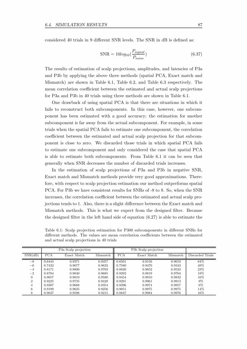
6.4. SIMULATION RESULTS 87
considered 40 trials in 9 different SNR levels. The SNR in dB is defined as:
SNR = 10log10(Psignal
Pnoise) (6.37)
The results of estimation of scalp projections, amplitudes, and latencies of P3a
and P3b by applying the above three methods (spatial PCA, Exact match and
Mismatch) are shown in Table 6.1, Table 6.2, and Table 6.3 respectively. The
mean correlation coefficient between the estimated and actual scalp projections
for P3a and P3b in 40 trials using three methods are shown in Table 6.1.
One drawback of using spatial PCA is that there are situations in which it
fails to reconstruct both subcomponents. In this case, however, one subcom-
ponent has been estimated with a good accuracy; the estimation for another
subcomponent is far away from the actual subcomponent. For example, in some
trials when the spatial PCA fails to estimate one subcomponent, the correlation
coefficient between the estimated and actual scalp projection for that subcom-
ponent is close to zero. We discarded those trials in which spatial PCA fails
to estimate one subcomponent and only considered the case that spatial PCA
is able to estimate both subcomponents. From Table 6.1 it can be seen that
generally when SNR decreases the number of discarded trials increases.
In the estimation of scalp projections of P3a and P3b in negative SNR,
Exact match and Mismatch methods provide very good approximations. There-
fore, with respect to scalp projection estimation our method outperforms spatial
PCA. For P3b we have consistent results for SNRs of -8 to 8. So, when the SNR
increases, the correlation coefficient between the estimated and actual scalp pro-
jections tends to 1. Also, there is a slight difference between the Exact match and
Mismatch methods. This is what we expect from the designed filter. Because
the designed filter in the left hand side of equation (6.27) is able to estimate the
Table 6.1: Scalp projection estimation for P300 subcomponents in different SNRs fordifferent methods. The values are mean correlation coefficients between the estimatedand actual scalp projections in 40 trials
P3a Scalp projection P3b Scalp projection
SNR(dB) PCA Exact Match Mismatch PCA Exact Match Mismatch Discarded Trials
−8 0.6444 0.9371 0.9357 0.6501 0.9156 0.9019 64%−6 0.7432 0.9677 0.9632 0.7580 0.9470 0.9343 48%−4 0.8171 0.9800 0.9703 0.8820 0.9652 0.9523 23%−2 0.8784 0.9840 0.9685 0.9292 0.9819 0.9704 18%0 0.9057 0.9810 0.9580 0.9454 0.9910 0.9832 16%2 0.9225 0.9735 0.9428 0.9291 0.9961 0.9913 9%4 0.9307 0.9688 0.9354 0.9296 0.9974 0.9957 6%6 0.9199 0.9625 0.9256 0.9051 0.9975 0.9975 14%8 0.9037 0.9598 0.9215 0.8847 0.9984 0.9976 16%

6.4. SIMULATION RESULTS 88
scaled scalp projection of one subcomponent, when we use the reference signals,
there is a change in that scale. In a low noise situation this has very little effect
(because of normalization of the left hand side of equation (6.27)).
However for P3a we have inconsistency in all methods. These inconsistencies
can be explained in terms of having 0.26 spatial correlation between the sub-
components. In Table 6.1 the increase in the correlation coefficient of the actual
and estimated P3a scalp projection with the increase in the noise level is mainly
because more noise can decrease the correlation between the subcomponents. In
Table 6.1, the noise effect in decreasing the correlation, and as a result, better
estimation can be seen in some ranges of SNRs for all the methods.
For confirmation of robustness we performed another experiment considering
two scalp projections which had a small spatial correlation of 0.1 and the results
were consistent for nearly all other methods. In Table 6.2 the mean and variance
of the ratio between the actual and estimated amplitudes in 40 trials are shown
considering all the methods. When SNR increases this ratio tends toward 1 for
all methods. In the amplitude estimation a bias can be seen for the Exact match
and Mismatch methods.
Regarding amplitude estimation, spatial PCA results in a better estimation.
In Table 6.3, the mean and variance of estimated latency in 40 trials is shown
considering the three methods. From this table, it can be seen that considering
Exact match method, the mean of estimated latency for P3a tends to 150 and
for P3b towards 200 with the increase in SNR. Also the variance of estimation
continuously decreases when the SNR increases. In the case of Mismatch, a bias
in latency estimation can be seen, however, the variance of estimation decreases
when the SNR increases.
Regarding latency estimation, the Exact match method outperforms the spa-
tial PCA and Mismatch methods. Since, with decrease in the SNR level, the
variance of estimation for spatial PCA increases, Mismatch method seems to
Table 6.2: Amplitude estimation for P300 subcomponents in different SNRs for differentmethods. The values are means and variances of the ratios between the actual andestimated amplitudes in 40 trials.
P3a Amplitude P3b Amplitude
SNR(dB) PCA Exact Match Mismatch PCA Exact Match Mismatch
−8 0.9872 ± 0.1130 1.9841 ± 0.1030 1.9882 ± 0.1785 1.3364 ± 0.1787 1.7276 ± 0.1506 1.8001 ± 0.1356−6 1.0130 ± 0.1000 1.6423 ± 0.1072 1.6691 ± 0.1030 1.3335 ± 0.0837 1.4022 ± 0.1436 1.4634 ± 0.1410−4 1.0857 ± 0.0873 1.5054 ± 0.0929 1.5434 ± 0.0909 1.4230 ± 0.1435 1.2766 ± 0.0922 1.3387 ± 0.0917−2 1.1309 ± 0.0708 1.3971 ± 0.0592 1.4509 ± 0.0508 1.4224 ± 0.1317 1.2119 ± 0.0796 1.2703 ± 0.07210 1.1349 ± 0.0540 1.3160 ± 0.0549 1.3857 ± 0.0648 1.3561 ± 0.1092 1.0941 ± 0.0688 1.1616 ± 0.06752 1.1179 ± 0.1110 1.2767 ± 0.0625 1.3534 ± 0.0630 1.2941 ± 0.0716 1.0239 ± 0.0416 1.0982 ± 0.04754 1.1302 ± 0.0301 1.2192 ± 0.0412 1.2956 ± 0.0437 1.2747 ± 0.0636 1.0012 ± 0.0459 1.0782 ± 0.04896 1.1085 ± 0.0703 1.2042 ± 0.0367 1.2858 ± 0.0406 1.2436 ± 0.0500 0.9668 ± 0.0296 1.0428 ± 0.02618 1.0927 ± 0.0538 1.1807 ± 0.0326 1.2678 ± 0.0381 1.2077 ± 0.0478 0.9464 ± 0.0282 1.0256 ± 0.0263

6.4. SIMULATION RESULTS 89
be more robust. If we evaluate and compare only Exact match and Mismatch
methods, we can see that the best approximation is for the scalp projections.
Therefore, in the case of Mismatch a bias in latency and amplitude estimation
can be seen. This is because we directly designed a filter for estimation of scalp
projections of one subcomponent considering two reference signals. Then, we
showed that in the case of having reference signals, which are not necessarily the
exact source signals, there is a scale change with no effect after normalization.
Therefore, the estimated scalp projection in the case of Mismatch in low noise
conditions is almost independent of the shape of reference signal. However, we
do not directly estimate the latencies and amplitudes of the subcomponents;
instead, we use the estimated scalp projections and some other cost functions
as shown in Algorithm 6.3. Therefore, in the case of Mismatch, the more the
reference signal is similar to the exact signal, the better estimation for latency
and amplitude is achieved.
Effect of real noise
In an experiment, we used 600ms pre-stimulus data as the background EEG
and used it as noise. Therefore, in SNR calculation the power of background
EEG is considered as the power of noise. For SNR close to 0, the results of
averaging over 40 trials are shown in Table 6.4.
The aim of this experiment was to compare the performance of three methods
in the case of having a non-Gaussian and non-linear noise which is more real-
istic. It can be seen that the Exact Match outperforms the Mismatch method
and both of them outperform PCA method. Also it seems that PCA method is
less robust in the case of having only background EEG as the noise.
Effect of reference mismatch
Table 6.3: Latency estimation for P300 subcomponents in different SNRs for differentmethods. The values are means and variances of the estimated latencies in 40 trials.
P3a Latency P3b Latency
SNR(dB) PCA Exact Match Mismatch PCA Exact Match Mismatch
−8 204.0667 ± 109.1588 153.3000 ± 2.6929 158.6333 ± 4.7885 187.2667 ± 42.0344 208.0333 ± 6.8857 193.5333 ± 10.9505−6 160.4333 ± 58.1903 154.6667 ± 2.0567 164.7000 ± 4.4346 199.5667 ± 31.1389 202.4333 ± 5.7816 184.6000 ± 8.4225−4 147.6000 ± 17.4111 154.6333 ± 1.9737 165.4667 ± 3.2667 217.7667 ± 24.8231 200.7333 ± 4.0166 182.2667 ± 6.3078−2 152.7000 ± 8.2927 153.6667 ± 1.5610 163.9000 ± 2.8569 213.2667 ± 19.6362 198.7667 ± 3.5495 184 ± 9.15760 148.2333 ± 6.7194 153.0667 ± 0.9072 163.6333 ± 2.1088 216.8667 ± 15.0143 197.3000 ± 4.0099 181.0333 ± 5.65982 150 ± 8.2838 151.9000 ± 0.8847 162.6000 ± 1.6316 213.8333 ± 19.8791 198.7333 ± 3.5227 189.5667 ± 14.88044 149.4000 ± 4.4458 151.2667 ± 0.6915 162.4333 ± 1.1651 220.2333 ± 13.9350 198.4000 ± 2.9431 208.4000 ± 14.48576 148.2667 ± 6.2474 150.7667 ± 0.5040 164.2667 ± 0.8277 217.8667 ± 13.7984 198.5667 ± 2.3146 218.0333 ± 1.18858 146.7667 ± 5.4815 150.4000 ± 0.4983 165.2333 ± 0.6261 216.8000 ± 10.7748 198.8667 ± 1.7564 219.2000 ± 0.6644

6.4. SIMULATION RESULTS 90
In Table 6.5 we tried to show the effects of different choices for reference sig-
nals. We changed the shape of P3a and P3b by changing their k and θ values in
equation (6.29) and generated different reference signals which are shown in Fig.
6.1 as dotted lines. From Table 6.5 it can be seen that with different degrees of
Mismatch we have different bias in estimation. When the Mismatch is very high
as it can be seen from the 15th row of Table 6.5, there is a high bias in latency
estimation. The estimations in Table 6.5 are the average estimation considering
15 trials at SNR 0. The bold row corresponds to our special reference choice for
P3a and P3b (presumed P3a and P3b in Fig. 6.1).
Effect of spatial correlation
In another experiment we kept the temporal correlation at 0.69 for P3a and
P3b as in Fig. 6.1. We then changed the locations and moments of P3a and P3b
in the brain in order to generate different levels of spatial correlations. In each
level, we generated 15 trials. By considering all the methods (and two different
SNR levels of -5 and 0), we calculated the average of correlation coefficients be-
tween the estimated and actual scalp projections which are shown in Fig. 6.3 for
both SNRs. The Exact match and Mismatch methods outperform the spatial
PCA in less than 0.9 spatial correlations. In both SNR levels the performances of
Exact match and Mismatch methods drop as the spatial correlation approaches
1. For spatial correlation less than 0.9, Exact match and Mismatch methods
outperform the spatial PCA.
Effect of temporal correlation
Our method is compared with temporal PCA from ERP PCA Toolkit [116]
in different temporal correlations considering two SNR levels of -5 and 0. In
temporal PCA algorithm, Promax is used as the rotation algorithm with the
rotation parameter 3, the relationship matrix type is covariance based, and the
loading normalization is Kaiser. The results are illustrated in Fig. 6.4. The spa-
tial correlation between the subcomponents is 0.26 and the result is the average
of the results for 15 trials. It is clear that the performance of the temporal PCA
Table 6.4: P300 subcomponents parameter estimation at SNR = 0 dB considering back-ground EEG as noise.
P3a P3b
Parameter PCA Exact Match Mismatch PCA Exact Match Mismatch
Scalp Projection 0.7044 0.8944 0.8614 0.8890 0.9620 0.9584Amplitude 0.7087 ± 0.0667 1.1759 ± 0.2063 1.1843 ± 0.2067 0.7968 ± 0.0306 0.9833 ± 0.1166 0.9600 ± 0.1263
Latency 136.0667 ± 19.8302 150.7000 ± 0.8367 165.6667 ± 2.2335 230.3667 ± 35.9976 200.6333 ± 3.6054 219.2333 ± 1.1943

6.5. REAL DATA RESULTS 91
degrades with the increase in the temporal correlation. In addition, low noise
situation has an adverse effect in temporal PCA. Clearly, our method, which
exploits both temporal and spatial domain and has no assumption on the un-
correlatedness or orthogonality of the subcomponents either in time or spatial
domain, outperforms the PCA/ICA based methods.
Finally, we tried to show a single trial estimation of scalp projection, ampli-
tude, and latency of P3a and P3b considering all three methods (spatial PCA,
Exact match and Mismatch). For these single trials, the latencies and amplitudes
of P3a and P3b change in different trials; therefore we have different temporal
correlations between P3a and P3b. In Fig. 6.5 the correlation coefficients of
estimated and actual scalp projections and latency estimation in the 30 single
trials are provided. In Fig. 6.6 the amplitude estimation is shown, in addition,
in this figure, the temporal correlation between P3a and P3b and SNR values in
each trial are shown. In the next section the method is applied to the real data
and the results are provided.
6.5 Real Data Results
The EEG data were recorded using a Nihon Kohden model EEG-F/G amplifier
and Neuroscan Acquire 4.0 software. The international 10 – 20 electrode setting
system was used to record EEG activity from 15 electrodes. The impedance for
all the electrodes was below 5kΩ. The sampling frequency (Fs) was 2kHz and
the data were bandpass filtered (0.1 – 70 Hz). This frequency range was chosen
to be consistent with [118]. In order to avoid any interference, the subjects were
required to sit alert with their eyes closed.
In addition, in order to avoid any muscle artefact, the neck was firmly sup-
ported by the back of the chair, feet were rested on a footstep, and stimuli
Table 6.5: Effects of Mismatch in P300 subcomponents descriptor’s estimation.
K - P3a K - P3b K P3a latency P3a amplitude P3a scalp K P3b Latency P3b amplitude P3b scalp
1 Fix decrease 22 156.3333 ± 1.0465 1.1814 ± 0.0532 0.9889 9 192.0667 ± 2.5204 1.2033 ± 0.0712 0.99222 Fix decrease 22 161.4667 ± 1.5055 1.1055 ± 0.0491 0.9892 4 190.5333 ± 2.0656 1.2641 ± 0.0695 0.99113 Fix increase 22 150.2667 ± 1.1629 1.2953 ± 0.0649 0.9619 19 208.1333 ± 4.1381 1.1752 ± 0.0846 0.99394 Fix increase 22 150.3333 ± 1.1751 1.3289 ± 0.0697 0.9496 24 213.6000 ± 2.9228 1.1705 ± 0.0865 0.9942
5 decrease Fix 17 155.2667 ± 0.9612 1.2618 ± 0.0619 0.9766 14 196.8000 ± 5.2807 1.1567 ± 0.0797 0.99146 decrease Fix 12 163.5333 ± 1.3020 1.3024 ± 0.0609 0.9753 14 189.6667 ± 5.2327 1.1015 ± 0.0757 0.99177 increase Fix 27 150.4000 ± 0.9103 1.2760 ± 0.0601 0.9766 14 198.3333 ± 4.5930 1.1522 ± 0.0786 0.99538 increase Fix 32 149.3333 ± 0.8997 1.2678 ± 0.0573 0.9765 14 197.7333 ± 4.6517 1.1688 ± 0.0806 0.9946
9 increase increase 27 148.3333 ± 1.1629 1.2909 ± 0.0621 0.9620 19 207.7333 ± 3.7315 1.1954 ± 0.0863 0.992010 increase increase 32 148.2000 ± 1.1464 1.3409 ± 0.0680 0.9498 24 211.9333 ± 2.8402 1.1616 ± 0.0856 0.994611 decrease decrease 17 160.2667 ± 1.3345 1.2794 ± 0.0543 0.9896 9 191.8000 ± 2.3361 1.1275 ± 0.0662 0.991212 decrease decrease 12 170.0000 ± 0 1.2229 ± 0.0510 0.9881 4 191.4000 ± 2.4437 1.2248 ± 0.0712 0.9901
13 decrease increase 17 153.0000 ± 1.0690 1.3481 ± 0.0635 0.9626 19 204.2000 ± 10.2901 1.0838 ± 0.0772 0.991114 decrease increase 12 159.0000± 1.4639 1.3561 ± 0.0696 0.9492 24 195.3333± 17.1159 1.0832± 0.0797 0.9916
15 decrease increase 7 170.0000 ± 0 1.4178 ± 0.0700 0.9419 27 180 ± 0 0.9834 ± 0.0750 0.958016 increase decrease 27 154.2000 ± 1.0823 1.1725 ± 0.0493 0.9891 9 191.4667 ± 2.5317 1.2178 ± 0.0715 0.989717 increase decrease 32 156.9333 ± 1.2799 1.0754 ± 0.0433 0.9895 4 188.8667 ± 2.1996 1.2820 ± 0.0688 0.9853

6.5. REAL DATA RESULTS 92
0.1 0.2 0.3 0.4 0.5 0.6 0.7 0.8 0.9 0.990
0.2
0.4
0.6
0.8
1
Spatial correlation
Corr
ela
tion C
oeffic
ient
Correlation coefficient between estimated andoriginal scalp projection for P3b (SNR = −5dB)
0.1 0.2 0.3 0.4 0.5 0.6 0.7 0.8 0.9 0.990
0.2
0.4
0.6
0.8
1
Spatial Correlation
Corr
ela
tion C
oeffic
ient
Correlation Coeffient between estimated and original Scalp Projections for P3a (SNR = −5dB)
0.1 0.2 0.3 0.4 0.5 0.6 0.7 0.8 0.9 0.990
0.2
0.4
0.6
0.8
1
Spatial Correlation
Corr
ela
tion C
oeffic
ient
Correlation coefficient between estimated and original scap projection for P3b (SNR = 0dB)
0.1 0.2 0.3 0.4 0.5 0.6 0.7 0.8 0.9 0.990
0.2
0.4
0.6
0.8
1
Spatial Correlation
Corr
ela
tion C
oeffic
ient
Correlation coefficient between estimated and original scalp projection for P3a (SNR = 0dB)
Spatial PCA
Exact Match
Mismatch
Spatial PCA
Exact Match
Mismatch
Spatial PCA
Exact Match
Mismatch
Spatial PCA
Exact Match
Mismatch
Figure 6.3: Comparison between three methods (spatial PCA, Exact Match and Mis-match) with respect to the correlation coefficient between the original and estimatedscalp projections of P3a (left column) and P3b (right column) in different spatial corre-lations and two SNR levels of -5 dB (top row) and 0 dB (bottom row).

6.5. REAL DATA RESULTS 93
0.1 0.2 0.3 0.4 0.5 0.6 0.7 0.8 0.90.980.4
0.5
0.6
0.7
0.8
0.9
1
Temporal Correlation
Corr
ela
tion C
oeffic
ient
Correlation coefficient between estimated and original scalp projections for P3a (SNR=0dB)
Temporal PCA
Exact Match
Mismatch
0.1 0.2 0.3 0.4 0.5 0.6 0.7 0.8 0.90.980.4
0.5
0.6
0.7
0.8
0.9
1
Temporal Correlation
Corr
ela
tion C
oeffic
ient
Correlation coefficient between estimated and original scalp projections for P3b (SNR=0dB)
Temporal PCA
Exact Match
Mismatch
0.1 0.2 0.3 0.4 0.5 0.6 0.7 0.8 0.90.980.2
0.4
0.6
0.8
1
Temporal Correlation
Corr
ela
tion C
oeffic
ient
Correlation coefficient between estimated and original scalp projections for P3a (SNR=−5dB)
Temporal PCA
Exact Match
Mismatch
0.1 0.2 0.3 0.4 0.5 0.6 0.7 0.8 0.90.980.2
0.4
0.6
0.8
1
Temporal Correlation
Corr
ela
tion C
oeffic
ient
Correlation coefficient between estimated and original scalp projections for P3b (SNR=−5dB)
Temporal PCA
Exact Match
Mismatch
Figure 6.4: Comparison between three methods (temporal PCA, Exact Match and Mis-match) with respect to the correlation coefficient between the original and estimatedscalp projections of P3a (left column) and P3b (right column) in different temporalcorrelations and two SNR levels of -5 dB (top row) and 0 dB (bottom row).

6.5. REAL DATA RESULTS 94
1 5 10 15 20 25 30
100
110
120
130
140
150
160
170
180
190
Trial Number
Late
ncy (
ms)
P3a Latency estimation
P3a actual value
Exact Match
Mismatch
Spatial PCA
1 5 10 15 20 25 30
160
180
200
220
240
260
280
300
320
Trial Number
Late
ncy (
ms)
P3b Latency estimation
P3b Actual Value
Exact Match
Mismatch
Spatial PCA
1 5 10 15 20 25 300.7
0.75
0.8
0.85
0.9
0.95
1
Trial Number
Corr
ela
tion c
oeffic
ient
Correlation coefficient of estimated andoriginal scalp projections for P3a
Spatial PCA
Exact Match
Mismatch
1 5 10 15 20 25 300.7
0.75
0.8
0.85
0.9
0.95
1
Trial Number
Corr
ela
tion c
oeffic
ient
Correlation coefficient of estimated and original scalp projection for P3b
Spatial PCA
Exact Match
Mismatch
Figure 6.5: In the top row, the correlation coefficient between the original and estimatedscalp projections of P3a and P3b obtained by the three methods (spatial PCA, ExactMatch and Mismatch) in each trial are shown. In the bottom row, single trial estimationof latencies of P3a and P3b obtained by the three methods (spatial PCA, Exact Matchand Mismatch) in each trial are shown.

6.5. REAL DATA RESULTS 95
1 5 10 15 20 25 30−0.5
0
0.5
1
1.5
2
2.5
3
3.5
Trial Number
SNR
(dB)
Signal to noise ratio values in different trials
1 5 10 15 20 25 300
0.2
0.4
0.6
0.8
1
Trial Number
Tem
pora
l cor
rela
tion
Temporal correlation of P3a and P3b in different trials
1 5 10 15 20 25 30
0.6
0.8
1
1.2
1.4
1.6
Trial Number
Ampl
itude
P3b Amplitudes in different trials
P3b Actual amplitude
Mismatch
Exact Match
Spatial PCA
1 5 10 15 20 25 30
0.2
0.4
0.6
0.8
1
1.2
1.4
1.6
1.8
Trial Number
Ampl
itude
P3a Amplitudes in different trials
P3a Actual amplitude
Exact Match
Mismatch
Spatial PCA
Figure 6.6: In the top row, single trial estimation of amplitudes of P3a and P3b obtainedby the three methods (spatial PCA, Exact Match and Mismatch) in each trial are shown.In the bottom row, SNR and temporal correlations between P3a and P3b in each trialare shown.
were presented through ear plugs inserted in the ear. Forty rare tones (1 kHz)
were randomly distributed amongst 160 frequent tones (2 kHz). Their intensity
was 65 dB with 10- and 50-milliseconds duration for rare and frequent tones,
respectively.
The subjects were asked to press a button as soon as they heard a low tone (1
kHz). Before the start of the experiment, the ability of the subject to distinguish
between low and high tones was confirmed. The basis of the designed task is to
assess basic memory processes. ERP components measured in this task included
N100, P200, N200, P3a and P3b. Forty trials from one subject related to the
infrequent (rare) tones were selected and the proposed method for estimation
of latency, amplitude and scalp projections of P3a and P3b was applied. These
trials and their average from channel Fz is shown in Fig. 6.7.
For selection of reference signals, we used the averaged P300 as it is shown
in Fig. 6.8. In the top row the selected reference signals have little overlap with
the average P300. The normalized estimated scalp projection using left hand
side of equation (6.27) is depicted for both P3a and P3b. It can be seen that
the scalp projection values for P3a are negative or very close to zero. This can
be explained from equation (6.27) because the term s1rT1 seems to be zero or
very close to zero. We slide the references (with slight changes in their shapes)

6.5. REAL DATA RESULTS 96
0 100 200 300 400 500 600 700−30
−20
−10
0
10
20
Time [ms]
Am
plit
ud
e
Single Trial ERPs from channel Fz
Averaged ERP
Figure 6.7: Single Trial ERPs (40 trials related to the infrequent tones) and their averagefrom channel Fz.
−0.5
0
0.5
−0.5
0
0.5
−0.5
0
0.5
−0.4
−0.2
0
0.2
0.4
−0.5
0
0.5
−0.5
0
0.5
100 150 200 250 300 350 400 450 500 550 600 650 700−10
−5
0
5
10
Am
plit
ude
Averaged P300
P3a reference
P3b reference
100 150 200 250 300 350 400 450 500 550 600 650 700−10
−5
0
5
10
Am
plit
ude
100 150 200 250 300 350 400 450 500 550 600 650 700−10
−5
0
5
10
Time [ms]
Am
plit
ude
Averaged P300
P3a reference
P3b reference
Averaged P300
P3a reference
P3b reference
P3a Scalp projection P3b Scalp projection
Figure 6.8: Selection of reference signals for P3a and P3b. In each row, the referencesignals for P3a and P3b with their estimated scalp projections are shown. By sliding thereference signals towards and away from the averaged P300 and varying their shapes, theobserved changes in their estimated scalp projections are helpful for reference selection.The reference signals shown in the middle row which have high correlation with theaveraged P300 are used as good candidates for approximating the actual P3a and P3b.

6.5. REAL DATA RESULTS 97
1 5 10 15 20 25 30 35 400
10
20
30
40
50
Trial Number
Am
plit
ud
e
Peak amplitude estimation in single trials
P3a
P3b
P3b Fitting
P3a Fitting
Figure 6.9: estimated amplitudes for P3a and P3b in different trials.
towards having more correlation with the average P300 as it is shown in the
middle row.
The estimated scalp projections seem to be more reasonable since they do
not contain only negative or very close to zero values. We can further slide
the references as it is shown in the bottom row and we can see that this time
the scalp projection for the second subcomponent has negative values in all the
entries. In the top row, the reference signal for P3a seems to have no correlation
(or very little correlation) with actual P3a so its estimated scalp projection has
negative or very close to zero values in all entries, however it seems that there
are some correlations between the reference signal and the actual signal for P3b.
In the bottom row, the reference signal for P3a seems to have overlap with the
actual P3b, therefore, in the first estimated subcomponent, P3b scalp projections
appeared. The reference signal for P3b seems to have no correlation with actual
P3b and the estimated scalp projection has negative values in all entries. It is
also possible to use arbitrary shapes for P3a and P3b to see which shapes are
more reasonable using the estimated scalp projections.
For our dataset, by testing different shapes for P3a and P3b, P3b shape was
more likely to be wider than P3a. We have used the selected reference signals
in middle row of Fig. 6.8 for P3a and P3b. After selecting the reference signals
we estimated the amplitude, latency, and scalp projections of P3a and P3b in
40 trials.
The amplitude variations of the P3a and P3b are shown in Fig. 6.9. We
fitted a polynomial with degree of 9 to P3a and P3b amplitudes in order to
see the total variability across trials. The mean latency of P3a was obtained as
283.3ms and the mean latency of P3b was obtained as 367.6ms. The estimated
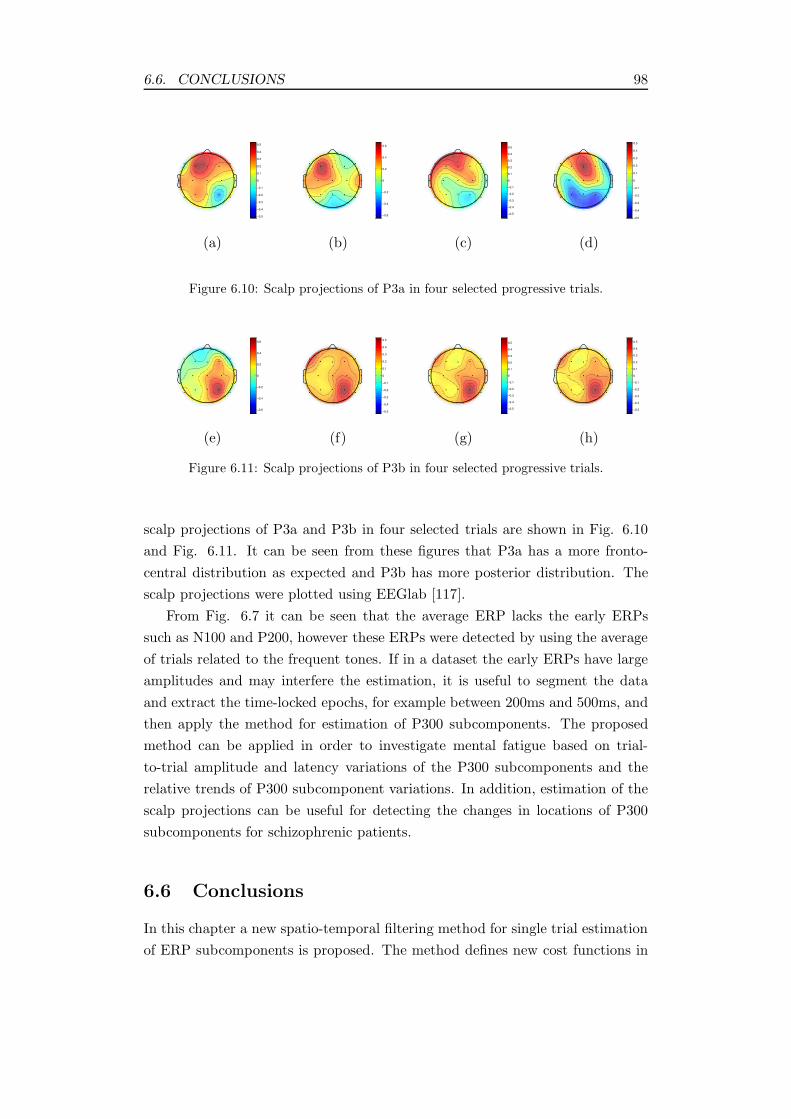
6.6. CONCLUSIONS 98
−0.5
−0.4
−0.3
−0.2
−0.1
0
0.1
0.2
0.3
0.4
0.5
−0.6
−0.4
−0.2
0
0.2
0.4
0.6
−0.5
−0.4
−0.3
−0.2
−0.1
0
0.1
0.2
0.3
0.4
0.5
−0.5
−0.4
−0.3
−0.2
−0.1
0
0.1
0.2
0.3
0.4
0.5
(a) (b) (c) (d)
Figure 6.10: Scalp projections of P3a in four selected progressive trials.
−0.6
−0.4
−0.2
0
0.2
0.4
0.6
−0.5
−0.4
−0.3
−0.2
−0.1
0
0.1
0.2
0.3
0.4
0.5
−0.5
−0.4
−0.3
−0.2
−0.1
0
0.1
0.2
0.3
0.4
0.5
−0.5
−0.4
−0.3
−0.2
−0.1
0
0.1
0.2
0.3
0.4
0.5
(e) (f) (g) (h)
Figure 6.11: Scalp projections of P3b in four selected progressive trials.
scalp projections of P3a and P3b in four selected trials are shown in Fig. 6.10
and Fig. 6.11. It can be seen from these figures that P3a has a more fronto-
central distribution as expected and P3b has more posterior distribution. The
scalp projections were plotted using EEGlab [117].
From Fig. 6.7 it can be seen that the average ERP lacks the early ERPs
such as N100 and P200, however these ERPs were detected by using the average
of trials related to the frequent tones. If in a dataset the early ERPs have large
amplitudes and may interfere the estimation, it is useful to segment the data
and extract the time-locked epochs, for example between 200ms and 500ms, and
then apply the method for estimation of P300 subcomponents. The proposed
method can be applied in order to investigate mental fatigue based on trial-
to-trial amplitude and latency variations of the P300 subcomponents and the
relative trends of P300 subcomponent variations. In addition, estimation of the
scalp projections can be useful for detecting the changes in locations of P300
subcomponents for schizophrenic patients.
6.6 Conclusions
In this chapter a new spatio-temporal filtering method for single trial estimation
of ERP subcomponents is proposed. The method defines new cost functions in

6.6. CONCLUSIONS 99
which the scalp projection of each subcomponent can be obtained. The proposed
method here overcomes the problem of the existence of temporal correlation
between the ERP subcomponents in the previous research [103].
Based on the simulation results the method is robust in the estimation of
latency, amplitude, and scalp projections. However, when there is a mismatch
between a reference signal and the actual source, an offset error in estimation
of the latency and amplitude occurs. This may not cause problems in some
applications. However, the scalp projections of both subcomponents have been
estimated with high accuracy even when there is a mismatch between the actual
source and the reference signal. This is obvious, because the designed filter for
estimation of the scalp projection is able to estimate the scaled scalp projection
of one of the subcomponents. When there is a mismatch between the actual
source and the reference signal, only the scale is changed. Therefore, the nor-
malized version of the estimated scalp projection vector does not change; this is
very important when we are dealing with localization of ERP subcomponents in
the brain. Using the simulated signals, it is shown that our proposed method
outperforms PCA/ICA based methods and a better approximation for scalp pro-
jections is obtained here. This leads to better localization of the subcomponents
in the brain which can be exploited in another research.
The method also has been applied to real data. It has been shown that it is
useful and effective for single trial estimation of P300 subcomponents. This is
very demanding for some applications such as mental fatigue where the relative
variability of ERP subcomponent descriptors is useful in order to determine the
level of fatigue.
Chapter 7
Implementation of EEG-based
and ERP-based Approaches to
Detection of Mental Fatigue;
an Auditory Based Paradigm
7.1 Introduction
In this chapter an auditory-based paradigm is proposed and implemented when
EEG data is recorded in two states of alert and fatigue. The EEG data is
recorded at the beginning of experiment while the subject is not fatigue. Then,
at the end of experiment when the subject has completed a mental arithmetic
task, EEG data is recorded in the fatigue state. The aim of this chapter is to
apply the proposed methods in the previous chapters for spatio-temporal esti-
mation of ERPs and EEG phase synchronization to the recorded EEG in an
auditory-based paradigm which can be used for detection of fatigue state. The
remainder of the chapter is structured as follows. In Section 7.2 the experimen-
tal setup is explained. Then, in Section 7.3 the results of applying the proposed
method in Chapter 6 to the recorded data is provided. In Section 7.4 the EEG
phase synchronization is estimated for the recorded data considering the pro-
posed method in Chapter 4. Finally, Section 7.5 concludes the chapter.
100

7.2. EXPERIMENTAL SETUP 101
7.2 Experimental Setup
The experiment was run in a quiet and normally illuminated room. The sub-
ject which was a 50 years old male was sitting comfortably in an armchair and
had given informed consent before the start of experiment. The EEG data was
recorded using a 32-channel QuickAmp amplifier and Ag/AgCl electrodes posi-
tioned according to the extended 10-20 system and re-referenced to linked ears.
In addition, vertical (VEOG) and horizontal (HEOG) electrooculographic sig-
nals were recorded bipolarly using electrodes above and below the left eye and
from the outer canthi. The EEG Data was recorded in DC mode at 1000 Hz
with respect to an average reference. The EEG data is also notch filtered at 50
Hz.
The electrode positions are shown in Fig. 7.1. By adding gel, electrode
impedances were reduced to less than 5kΩ. The EEG signal was recorded at the
start of the experiment during the auditory oddball task. The subject heard 180
tones, 40 of them were infrequent tones while 140 of them were frequent tones.
The subject was asked to respond to the infrequent tones by pressing a button.
Each trial duration was set to 4 seconds.
After completing the initial recoding of the EEG, the subject was asked to
perform a mental arithmetic task continuously for two hours. The subject had
also the option of stopping the mental arithmetic task if he felt that he is very
tired and is not willing to continue. The Matlab software was used to provide
a demo which generates two random integers between 1 and 10. The subject
had to enter the sum of the generated random numbers and then press ENTER
key on the keyboard or ‘Submit’ button in the demo. The demo is shown in
Fig. 7.2. After 2 hours performing the arithmetic task, the EEG data of the
subject was recorded during the same auditory oddball task in the beginning of
the experiment. In the next two sections the results of applying the proposed
methods in Chapters 6 and 4 to the recorded EEG signal are provided.
7.3 Estimation of Single Trial P300 Subcomponents
Considering the results provided in Chapter 6, it is expected the P300 to be
better elicited by infrequent tones. Therefore, using the spatio-temporal filtering
method proposed in Chapter 6, it is possible to estimate P300 subcomponent
parameters and evaluate their changes during the fatigue state considering the
infrequent tones. The spatio-temporal filtering method was applied to the 40
trials relating to the infrequent tones in order to estimate P300 subcomponent
parameters. One second of EEG signal after the stimulus onset in infrequent

7.3. ESTIMATION OF SINGLE TRIAL P300 SUBCOMPONENTS 102
Figure 7.1: The electrode names (left) and numbers (right) which used in the experiment.
Figure 7.2: This GUI generates two random integers any time the subject presses EN-TER key on the keyboard or ‘Submit’ button.

7.3. ESTIMATION OF SINGLE TRIAL P300 SUBCOMPONENTS 103
trials was segmented. The average of these trials (considering 600ms) from Cz
channel was used in order to select appropriate reference signals. Forty single
trial ERPs from channel Cz and their average before and during fatigue are
shown in Fig. 7.3 and Fig. 7.4 respectively. The two averaged ERPs are shown
separately in Fig. 7.5 for the two states of before and during fatigue. These
average ERPs are used in order to select an appropriate reference signal for P3a
and P3b. As it is shown in Chapter 6, the reference signals should have high
correlation with the averaged ERP.
It can be seen from the averaged ERPs that as expected in the fatigue state
there is a reduced amplitude and increased latency in the P300 wave. However
the reduction in amplitude is very trivial and this is not always a sign of fatigue
state. In addition the increased latency does not necessary correspond to the
increased latency in all single trials since it is averaged over only one channel
considering 40 trials. Therefore, there is a need for single trial estimation of the
ERPs.
The spatio-temporal filtering method proposed in Chapter 6 is applied to the
single trial ERPs before and during fatigue state to estimate P300 subcomponent
descriptors (latency, amplitude, and scalp projections). The mean latency of P3a
and P3b before fatigue state was obtained as 279.6 ms and 335.5 ms respectively.
The mean latency of P3a and P3b during fatigue state was obtained as 325.5 ms
and 372.2 ms respectively. As expected, the latency of P3a and P3b are increased
in the fatigue state. The estimated amplitudes of P3a and P3b are shown in Fig.
7.6 and Fig. 7.7. By fitting a polynomial of degree 10 to the estimated P3a and
P3b amplitudes before and during fatigue state, it can be seen that in the fatigue
state there is a less variability in P3a and P3b amplitudes in single trials. The
scalp projections of P3a and P3b for five selected trials are shown in Fig. 7.8
and Fig. 7.9 for before and during fatigue state respectively.
Although there is not a significant difference in the estimated scalp projec-
tions for P3a and P3b before and during fatigue state, the important issue is the
separation of these subcomponents and estimation of other parameters. The re-
sults obtained by considering one subject confirm that the suggested paradigm
can be a good option for designing a mental fatigue detection system in fu-
ture studies and the estimation of P300 subcomponent parameters can be good
features for discriminating the fatigue state. However, the full mental fatigue
analysis should be conducted using more subjects and more features which can
be obtained from both EEG and ERP. Other important features can be obtained
using phase synchronization measures. In the next section, the proposed adap-
tive methods in Chapter 4 are used to measure the EEG phase synchronization
to the recorded EEG data.

7.3. ESTIMATION OF SINGLE TRIAL P300 SUBCOMPONENTS 104
0 100 200 300 400 500 600−20
−15
−10
−5
0
5
10
15
20
Sample Number
Am
plit
ud
e
Averaged ERP before fatigue
Figure 7.3: Forty single trial ERPs and their average from Cz channel before fatigue.
0 100 200 300 400 500 600−20
−15
−10
−5
0
5
10
15
20
Sample Number
Am
plit
ud
e
Averaged ERP during fatigue
Figure 7.4: Forty single trial ERPs and their average from Cz channel during fatiguestate.
0 100 200 300 400 500 600−8
−6
−4
−2
0
2
4
Sample Number
Am
plit
ud
e
Averaged ERP during fatigue
Averaged ERP before fatigue
Figure 7.5: The averaged ERP of forty trials before and during fatigue state from Czchannel.

7.3. ESTIMATION OF SINGLE TRIAL P300 SUBCOMPONENTS 105
1 5 10 15 20 25 30 35 400
10
20
30
40
50
60
Trial Number
Am
plit
ude
P3a during fatigue
P3a fitting during fatigue
P3a before fatigue
P3a fitting before fatigue
Figure 7.6: The estimated P3a amplitudes in single trials before and during fatiguestate.
0 5 10 15 20 25 30 35 400
10
20
30
40
50
60
70
80
90
100
Trial Number
Am
plit
ud
e
P3b during fatigue
P3b fitting during fatigue
P3b before fatigue
P3b fitting before fatigue
Figure 7.7: The estimated P3b amplitudes in single trials before and during fatiguestate.
Figure 7.8: The estimated scalp projections of P3a (top row) and P3b (bottom row)before fatigue.
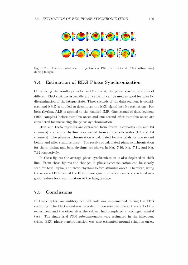
7.4. ESTIMATION OF EEG PHASE SYNCHRONIZATION 106
Figure 7.9: The estimated scalp projections of P3a (top row) and P3b (bottom row)during fatigue.
7.4 Estimation of EEG Phase Synchronization
Considering the results provided in Chapter 4, the phase synchronizations of
different EEG rhythms especially alpha rhythm can be used as good features for
discrimination of the fatigue state. Three seconds of the data segment is consid-
ered and EMD is applied to decompose the EEG signal into its oscillations. For
beta rhythm, ALE is applied to the resulted IMF. One second of data segment
(1000 samples) before stimulus onset and one second after stimulus onset are
considered for measuring the phase synchronization.
Beta and theta rhythms are extracted from frontal electrodes (F3 and F4
channels) and alpha rhythm is extracted from central electrodes (C3 and C4
channels). The phase synchronization is calculated for five trials for one second
before and after stimulus onset. The results of calculated phase synchronization
for theta, alpha, and beta rhythms are shown in Fig. 7.10, Fig. 7.11, and Fig.
7.12 respectively.
In these figures the average phase synchronization is also depicted in thick
line. From these figures the changes in phase synchronization can be clearly
seen for beta, alpha, and theta rhythms before stimulus onset. Therefore, using
the recorded EEG signal the EEG phase synchronization can be considered as a
good feature for discrimination of the fatigue state.
7.5 Conclusions
In this chapter, an auditory oddball task was implemented during the EEG
recording. The EEG signal was recorded in two sessions, one at the start of the
experiment and the other after the subject had completed a prolonged mental
task. The single trial P300 subcomponents were estimated in the infrequent
trials. EEG phase synchronization was also estimated around stimulus onset.
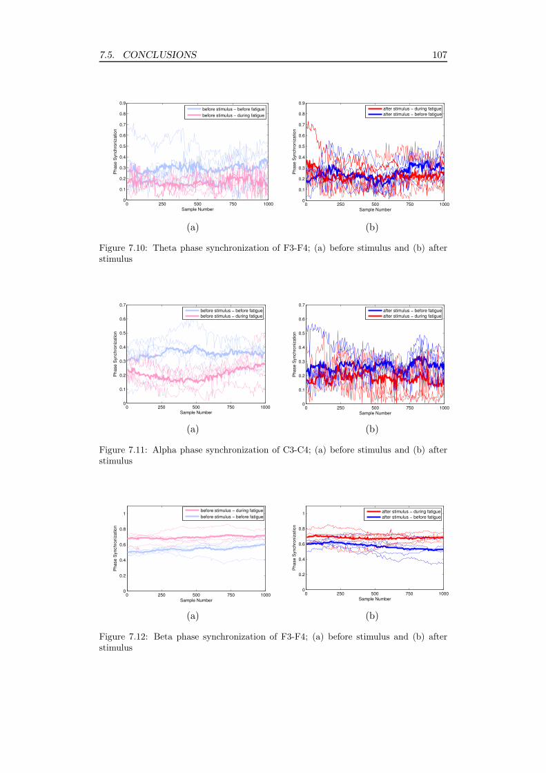
7.5. CONCLUSIONS 107
0 250 500 750 10000
0.1
0.2
0.3
0.4
0.5
0.6
0.7
0.8
0.9
Sample Number
Ph
ase
Syn
ch
ron
iza
tio
n
before stimulus − before fatigue
before stimulus − during fatigue
0 250 500 750 10000
0.1
0.2
0.3
0.4
0.5
0.6
0.7
0.8
0.9
Sample Number
Ph
ase
Syn
ch
ron
iza
tio
n
after stimulus − during fatigue
after stimulus − before fatigue
(a) (b)
Figure 7.10: Theta phase synchronization of F3-F4; (a) before stimulus and (b) afterstimulus
0 250 500 750 10000
0.1
0.2
0.3
0.4
0.5
0.6
0.7
Sample Number
Ph
ase
Syn
ch
ron
iza
tio
n
before stimulus − before fatigue
before stimulus − during fatigue
0 250 500 750 10000
0.1
0.2
0.3
0.4
0.5
0.6
0.7
Sample Number
Ph
ase
Syn
ch
ron
iza
tio
n
after stimulus − before fatigue
after stimulus − during fatigue
(a) (b)
Figure 7.11: Alpha phase synchronization of C3-C4; (a) before stimulus and (b) afterstimulus
0 250 500 750 10000
0.2
0.4
0.6
0.8
1
Sample Number
Ph
ase
Syn
ch
ron
iza
tio
n
before stimulus − during fatigue
before stimulus − before fatigue
0 250 500 750 10000
0.2
0.4
0.6
0.8
1
Sample Number
Ph
ase
Syn
ch
ron
iza
tio
n
after stimulus − during fatigue
after stimulus − before fatigue
(a) (b)
Figure 7.12: Beta phase synchronization of F3-F4; (a) before stimulus and (b) afterstimulus

7.5. CONCLUSIONS 108
The results demonstrate the effectiveness of applying the methods for the odd-
ball paradigm which can be considered as a vigilance test for detection of the
fatigue state. In addition by applying the proposed methods for spatio-temporal
estimation of P300 subcomponents and EEG phase synchronization, the results
demonstrate the use of estimated EEG phase synchronization and single trial
P300 subcomponents as appropriate and effective features for the analysis and
understanding of mental fatigue.

Chapter 8
Summary, Conclusions and
Future Works
8.1 Summary and Conclusions
Over the past decade, there has been increasing scientific interest in detection
of mental fatigue state. However the research in mental fatigue analysis using
EEG signals has been limited to classical methods whereby simple features from
the signals are compared or classified. In addition the analysis of mental fatigue
cannot be completed using only one type of biometric. The general strategy in
a mental fatigue detection system is to fuse as many features as possible. These
features can be obtained from different kinds of input signals (e.g. EEG, ECG)
and it is important to extract features which are most relevant. After designing
the mental fatigue detection system, an alarming signal may be produced to
indicate the warning of the fatigue state and prevent accidents.
In this study, analysis of mental fatigue is conducted by following two impor-
tant directions. One direction is using EEG signal and extracting its effective
features related to EEG phase synchronization. The other direction is using the
ERP signal and estimating its parameters in single trials. New methods for each
direction have been proposed in this study.
In the traditional methods, average ERP is used for evaluating the changes in
the ERP signal before and during fatigue state. However the average ERP does
not always correspond to the appearance of mental fatigue since the averaging
results in loss of information related to the trial to trial variability of ERPs.
The inter-trial variability of ERPs can change in the fatigue state. Therefore,
109

8.1. SUMMARY AND CONCLUSIONS 110
there is an essential need to apply the single trial-based method for estimation
of ERPs. In this study, two methods for single trial estimation of ERPs have
been proposed. One of them is a temporal method based on RBPF and the other
one a spatio-temporal filtering method based on constrained optimization. In the
temporal method, tracking of the ERPs in single trials has been considered while
in the spatio-temporal filtering method ERPs are estimated in both spatial and
temporal domains. In addition, the designed spatio-temporal filtering method
has been shown to be robust against both temporal and spatial correlations
between the ERP subcomponents.
For analysis of mental fatigue based on EEG signals, classical methods calcu-
late power spectrum of EEG in different frequency bands before and during the
fatigue state. To account for non-stationarity of the EEG signals, there is a need
for application of the recent adaptive methods which are suitable for analysing
non-stationary and non-linear signals. These methods include EMD and ALE.
In addition it is beneficial to measure synchronization of the brain activity in
different brain regions. EMD and ALE have been proposed for decomposing the
EEG signals into their oscillations and then denoising them. The phase syn-
chronization of different EEG oscillations over different parts of the brain are
calculated to observe the changes in the fatigue state. In addition, the RBPF
was proposed for estimation of instantaneous phase of an EEG oscillation. The
method has provided a new insight into the estimation of instantaneous phase
which can be extended for measuring phase synchronization in future studies.
The effect of mental fatigue relates to reduced performance and decreased
vigilance [119]. Through designing a vigilance test based paradigm it is possible
to detect the changes in the vigilance state of the subject during the fatigue
state. Auditory reaction time can be used as an objective assessment of vigilance.
Therefore, in Chapter 7 an auditory based paradigm has been used. Based on the
proposed paradigm, at the beginning of the experiment a vigilance test is taken
from the subject using an oddball task. Then, at the end of experiment, when
the subject has completed a prolonged mental task, the vigilance test is taken
again. The proposed methods have been applied to estimate the single trial P300
subcomponents and the EEG phase synchronization. The results demonstrate
the effectiveness of using the auditory oddball paradigm in a mental fatigue
detection system.

8.2. FUTURE WORKS 111
8.2 Future Works
The new methods proposed in this study for estimation of single trial ERPs
and EEG phase synchronization can be used for extracting reliable features in
a mental fatigue detection system. As it is emphasized in this study, compre-
hensive analysis of mental fatigue cannot be performed by relying on only few
features. In future studies, a classifier or a regression method can be used for
online detection of mental fatigue state considering the features that must be
obtained by applying the proposed methods in this study and also considering
more subjects.
The proposed method in Chapter 4 which combines EMD and RBPF and
estimates the instantaneous phase of the EEG oscillation should be further ex-
tended in order to estimate the EEG phase synchronization in real time effec-
tively. Since this method uses RBPF with several constraints, the parameters
should be selected appropriately and a reasonable number of particles should be
used for the method to be applicable in real time situations.
The proposed methods in this thesis can be used for the study of driver
fatigue. One of the major causes for driver fatigue based accidents is sleepiness
[120]. Since sleepiness or drowsiness reduces the reaction time and as the result
the vigilance state of the driver, the suggested auditory paradigm and estimation
of ERPs can be used in a driver fatigue detection scenario.
In some research, especially in driver fatigue, different types of fatigue are of-
ten considered the same and the drowsiness level of the driver or his/her fatigue
state is estimated. However, it is very crucial to distinguish between task-related
fatigue and sleep related fatigue by designing appropriate assessment or record-
ing paradigms. For example, in a paradigm for detection of mental fatigue, only
mental task related fatigue should be included and for the paradigm in sleepiness
detection both sleepiness and mental task effect should be considered. Evalua-
tion of mental fatigue can also depend on subject, age, sex, any possible brain
abnormality, recording time, environment, emotional and social engagement, and
many other parameters. A robust fatigue monitoring system should indeed take
all these factors into account.

Bibliography
[1] M. A. S. Boksem, T. F. Meijman, and M. M. Lorist. Effects of mental
fatigue on attention: an ERP study. Cognitive Brain Research, 25:107–
116, 2005.
[2] E. Niedermeyer and F. L. Da Silva. Electroencephalography: Basic prin-
ciples, clinical applications, and related fields. Lippincott Williams and
Wilkins, 1999.
[3] J. M. Stern and J. Engel. Atlas of EEG patterns. Lippincott Williams and
Wilkins, 2004.
[4] S. Makeig, A. J. Bell, T. P. Jung, and T. J. Sejnowski. Independent com-
ponent analysis of electroencephalographic data. Adv. Neural Inf. Proc.
Syst., 8:145–151, 1996.
[5] M. M. Ter-Pogossian, M. E. Phelps, E. J. Hoffman, and N. A. Mullani. A
positron-emission transaxial tomograph for nuclear imaging (PET). Radi-
ology, 114(1):89–98, 1975.
[6] J. W. Belliveau, D. N. Kennedy, R. C. McKinstry, B. R. Buchbinder,
R. M. Weisskoff, M. S. Cohen, J. M. Vevea, T. J. Brady, and B. R. Rosen.
Functional mapping of the human visual cortex by magnetic resonance
imaging. Science, 254:716–719, 1991.
[7] J. Clarke and A. I. Braginski. The SQUID Handbook, volume 1. Wiley-Vch,
2004.
[8] W. G. Walter and M. A. Camb. The location of cerebral tumours by
electro-encephalography. Lancet, 228:305–308, 1936.
[9] W. G. Walter and V. J. Dovey. Electro-encephalography in cases of sub-
cortical tumour. J. Neurol. Neurosurg. Psychiat., 7:57–65, 1944.
112

BIBLIOGRAPHY 113
[10] E. Kirmizi-Alsan, Z. Bayraktaroglu, H. Gurvit, Y. H. Keskin, M. Emre,
and T. Demiralp. Comparative analysis of event-related potentials during
Go/NoGo and CPT: decomposition of electrophysiological markers of re-
sponse inhibition and sustained attention. Brain Res., 1104(1):114–128,
2006.
[11] T. Ishihara and N. Yoshii. Multivariate analytic study of EEG and mental
activity in juvenile delinquents. Electroencephalogr. Clin. Neurophysiol.,
33(1):71–80, 1972.
[12] Y. Mizuki, M. Tanaka, H. Isozaki, H. Nishijima, and K. Inanaga. Periodic
appearance of theta rhythm in the frontal midline area during performance
of a mental task. Electroencephalogr. Clin. Neurophysiol., 49(3-4):345–351,
1980.
[13] Y. Mizuki. Frontal lobe: mental functions and EEG. Am. J. EEG Technol.,
27:91–101, 1987.
[14] G. E. Chatrian, L. Bergamini, and M. Dondey. A glossary of terms most
commonly used by clinical electroencephalographers. Electroencephalogr.
Clin. Neurophysiol., 37(5):538–548, 1974.
[15] E. Niedermeyer, G. L. Krauss, and C. E. Peyser. The electroencephalogram
and mental activation. Clin. Electroencephalogr., 20(4):215–227, 1989.
[16] G. E. Chatrian, M. C. Petersen, and J. A. Lazarte. The blocking of the
rolandic wicket rhythm and some central changes related to movement.
Electroencephalogr. Clin. Neurophysiol., 11(3):497–510, 1959.
[17] D. Klass and R. Bickford. Observations on the rolandic arceau rhythm.
Electroencephalogr. Clin. Neurophysiol., 9:570, 1957.
[18] S. Arroyo, R. P. Lesser, B. Gordon, S. Uematsu, D. Jackson, and R. Web-
ber. Functional significance of the mu rhythm of human cortex: an elec-
trophysiologic study with subdural electrodes. Electroencephalogr. Clin.
Neurophysiol., 87(3):76–87, 1993.
[19] G. Pfurtscheller and C. Neuper. Simultaneous EEG 10 Hz desynchroniza-
tion and 40 Hz synchronization during finger movements. Neuroreport.,
3(12):1057–1060, 1992.
[20] G. Pfurtscheller, D. Flotzinger, and C. Neuper. Differentiation between
finger, toe and tongue movement in man based on 40 Hz EEG. Electroen-
cephalogr Clin Neurophysiol., 90(6):456–460, 1994.

BIBLIOGRAPHY 114
[21] S. J. Luck. An Introduction to the Event-Related Potential Technique.
Cambridge, Mass.: The MIT Press, 2005.
[22] J. Polich. Updating P300: an integrative theory of P3a and P3b. Clin.
Neurophysiol., 118(10):2128–2148, 2007.
[23] R. Johnson. On the neural generators of the P300 component of the event-
related potential. Psychophysiology, 30:90–97, 1993.
[24] W. R. Hensyl. Stedman’s Medical Dictionary. Williams and Wilkins, Bal-
timore, MD, 25th edition, 1990.
[25] E. Grandjean. Fitting the Task to the Man. London: Taylor and Francis.
[26] G. Kecklund and T. Akerstedt. Sleepiness in long distance truck driving:
An ambulatory EEG study of night driving. Ergonomics, 36:1007–1017,
1993.
[27] K. A. Brookhius and D. D. Waard. The use of psychophysiology to assess
driver status. Ergonomics, 36(2):1099–1110, 1993.
[28] D. D. Waard and K. A. Brookhius. Assessing driver status: A demonstra-
tion experiment on the road. Accident Analysis and Prevention, 23:297–
307, 1991.
[29] D. F. Dinges. An overview of sleepiness and accidents. J. Sleep Res.,
4(S2):4–14, 1995.
[30] M. M. Mitler, M. A. Carskadon, C. A. Czeisler, W. C. Dement, D. F.
Dinges, and R. C. Graeber. Catastrophes, sleep and public policy an
overview of sleepiness and accidents. Consensus report. Sleep, 11:100–109,
1988.
[31] T. A. Dingus, S. G. Klauer, V. L. Neale, A. Petersen, S. E. Lee, J. Sud-
weeks, M. A. Perez, J. Hankey, D. Ramsey, S. Gupta, C. Bucher, Z. R.
Doerzaph, J. Jermeland, and R. R. Knipling. The 100-car naturalistic
driving study, phase II results of the 100-Car field experiment (DOT HS
810 593). Washington, DC: U.S. Department of Transportation, National
Highway Traffic Safety Administration, 2006.
[32] S. Sanei and J. Chambers. EEG signal Processing. John Wiley and Sons,
2007.

BIBLIOGRAPHY 115
[33] I. A. Cook, R. O’Hara, S. H. J. Uijtdehaage, M. Mandelkern, and A. F.
Leuchter. Assessing the accuracy of topographic EEG mapping for de-
termining local brain function. Electroencephalogr. Clin. Neurophysiol.,
107:408–414, 1998.
[34] A. Beyerle E. Eger A. Salek-Haddadi C. Preibisch H. Laufs, A. Klein-
schmidt and K. Krakow. EEG-correlated fMRI of human alpha activity.
NeuroImage, 19:1463–1476, 2003.
[35] R. D. Ogilvie. Physiological review: the process of falling asleep. Sleep
Medicine Reviews, 5(3):247–270, 2001.
[36] S. K. L. Lal and A. Craig. A critical review of the psychophysiology of
driver fatigue. Biological Psychology, 55:173–194, 2001.
[37] C. Lafrance and M. Dumont. Diurnal variations in the waking EEG: com-
parison with sleep latencies and subjective alertness. J. Sleep Res., 9:243–
248, 2000.
[38] W. Klimesh. EEG alpha and theta oscillations reflect cognitive and mem-
ory performance: a review and analysis. Brain Res. Rev., 29:169–195,
1999.
[39] B. S. Oken and M. Salinsky. Alertness and attention: basic science and
electrophysiologic correlates. J. Clin. Neurophysiol, 9(4):480–494, 1992.
[40] K. Q. Shen, X. P. Li, W. L. P. M. Pullens, H. Zheng, C. J. Ong, and
E. P. V. Wilder-Smith. Key feature extraction for fatigue identification
using random forests. Proceedings of the 27th Annual IEEE Conference on
Engineering in Medicine and Biology, 2005.
[41] A. Muzur, E. F. Pace-Schott, and J. A. Hobson. The prefrontal cortex in
sleep. Electroencephalogr. Clin. Neurophysiol., 6:475–481, 2002.
[42] L. Breiman. Random forests. Machine Learning, 45:5–32, 2001.
[43] I. Guyon, S. Gunn, A. B. Hur, and G. Dror. Result analysis of the NIPS
2003 feature selection challenge. Proceedings of the Eighteenth Annual Con-
ference on Neural Information Processing Systems, Vancouver, Canada,
2004.
[44] K. Q. Shen, C. J. Ong, X. P. Li, Z. Hui, and E. P. V.Wilder-Smith. A
feature selection method for multilevel mental fatigue EEG classification.
IEEE Trans. Biomed. Eng., 54(7):1231–1237, 2007.

BIBLIOGRAPHY 116
[45] A. V. Oppenheim and R. W. Schafer. Discrete-Time Signal Processing.
Upper Saddle River, NJ: Prentice-Hall, 1989.
[46] A. Lempel and J. Ziv. On the complexity of finite sequence. IEEE Trans-
actions on Information Theory, 22:75–81, 1976.
[47] S. M. Pincus. Approximate entropy as a measure of system complexity.
Proceedings of the National Academy of Science United States of America,
88:2297–2301, 1991.
[48] I. A. Rezek and S. J. Roberts. Stochastic complexity measures for phys-
iological signal analysis. IEEE Transactions on Biomedical Engineering,
45(9):1186–1191, 1998.
[49] J. Liu, C. Zhang, and C. Zheng. EEG-based estimation of mental fatigue
by using KPCA-HMM and complexity parameters. Biomedical Signal Pro-
cessing and Control, Elsevier, 5(2):124–130, 2010.
[50] B. Scholkopf, A. J. Smola, and K. R. Muller. Nonlinear component analysis
as a kernel eigenvalue problem. Neural Computation, 10:1299–1319, 1998.
[51] K. R. Muller, S. Mika, G. Ratsch, K. Tsuda, and B. Scholkopf. An intro-
duction to kernel-based learning algorithms. IEEE Transactions on Neural
Networks, 12:181–201, 2001.
[52] L. R. Rabiner. A tutorial on hidden markov models and selected applica-
tions in speech recognition. Proceedings of the IEEE, 77(2):257–286, 1989.
[53] F. Varela, J. P. Lachaux, E. Rodriguez, and J. Martinerie. The brainweb:
phase synchronization and large-scale integration. Nat. Rev. Neurosci.,
2(4):229–239, 2001.
[54] N. E. Huang, Z. Shen, S. R. Long, M. C. Wu, H. H. Shih, Q. Zheng,
N. C. Yen, C. C. Tung, and H. H. Liu. The empirical mode decomposition
and hilbert spectrum for nonlinear and non-stationary time series analysis.
Proc Roy Soc London A, 454:903–995, 1998.
[55] S. Haykin. Adaptive filter theory. Prentice-Hall, New Jersey, 2002.
[56] P. Wagner, J. Roschke, J. Fell, and C. Frank. Differential pathophysio-
logical mechanisms of reduced P300 amplitude in schizophrenia and de-
pression: a single trial analysis. Schizophrenia Research, 25(3):221–229,
1997.
BIBLIOGRAPHY 117
[57] P. Wagner, J. Roschke, M. Grozinger, and K. Mann. A replication study
on P300 single trial analysis in schizophrenia: confirmation of a reduced
number of ’true positive’ P300 waves. J. Psychiatr. Res., 34(3):255–259,
2000.
[58] S. Cerutti, V. Bersani, A. Carrara, and D. Liberati. Analysis of visual
evoked potentials through wiener filtering applied to a small number of
sweeps. J. Biomed. Eng., 9(1):3–12, 1987.
[59] W. Truccolo, K. H. Knuth, A. Shah, S. L. Bressler, C. E. Schroeder, and
M. Ding. Estimation of single-trial multicomponent ERPs: Differentially
variable component analysis (DVCA). Biol. Cybern., 89(6):426–438, 2003.
[60] M. V. Spreckelsen and B. Bromm. Estimation of single-evoked cerebral
potentials by means of parametric modeling and kalman filtering. IEEE
Trans. Biomed. Eng., 35(9):691–700, 1988.
[61] S. D. Georgiadis, P. O. Ranta-aho, M. P. Tarvainen, and P. A. Karjalainen.
Single-trial dynamical estimation of event-related potentials: a kalman
filter-based approach. IEEE Trans. Biomed. Eng., 52(8):1397–1406, 2005.
[62] R. M. Chapman and J. W. McCrary. EP component identification and
measurement by principal components analysis. Brain Cogn., 27(3):288–
310, 1995.
[63] A. C. Tang, B. A. Pearlmutter, N. A. Malaszenko, D. B. Phung, and B. C.
Reeb. Independent components of magnetoencephalography: Localization.
Neural Comput., 14(8):1827–1858, 2002.
[64] M. Zibulevsky and Y. Y. Zeevi. Extraction of a single source from mul-
tichannel data using sparse decomposition. Neurocomputing, 49:163–173,
2002.
[65] X. Wang, Y. Chen, and M. Ding. Estimating granger causality after stim-
ulus onset: A cautionary note. NeuroImage, 41(3):767–776, 2008.
[66] N. Fogelson, X. Wang, J. B. Lewis, M. M. Kishiyama, M. Ding, and R. T.
Knight. Multimodal effects of local context on target detection: evidence
from P3b. J. Cogn. Neurosci., 21(9):1680–1692, 2009.
[67] L. Xu, P. Stoica, J. Li, S. L. Bressler, X. Shao, and M. Ding. ASEO: A
method for the simultaneous estimation of single-trial event-related poten-
tials and ongoing brain activities. IEEE Trans. Biomed. Eng., 56(1):111–
121, 2009.

BIBLIOGRAPHY 118
[68] H. R. Mohseni, K. Nazarpour, E. Wilding, and S. Sanei. Application of
particle filters in single-trial event related potential estimation. Physiolog-
ical Measurements, 30(10):1101–1116, 2009.
[69] A. Murata and A. Uetake. Evaluation of mental fatigue in human-computer
interaction-analysis using feature parameters extracted from event-related
potential. Proceedings of 10th IEEE International Workshop on Robot and
Human Interactive Communication, pages 630–635, 2001.
[70] A. Murata, A. Uetake, and Y. Takasawa. Evaluation of mental fatigue us-
ing feature parameter extracted from event-related potential. International
Journal of Industrial Ergonomics, 35(8):761–770, 2005.
[71] U. Neumann, P. Ullsperger, H. G. Gille, and M. Pietschann. Effects of
graduated processing difficulty on P300 component of the event-related
potential. Psychology, 194:25–37, 1986.
[72] P. Ullsperger, A. M. Metz, X. Yu, and H. G. Gille. The P300 component of
the event-related brain potential and mental effort. Ergonomics, 31:1127–
1137, 1988.
[73] P. Ullsperger, U. Neumann, H. G. Gille, and M. Pietschann. P300 com-
ponent of ERP as an index of processing difficulty. Human Memory and
Cognitive Capabilities, pages 723–731, 1986.
[74] C. Zhang, C. Zheng, X. Yu, and Y. Ouyang. Estimating VDT mental
fatigue using multichannel linear descriptors and KPCA-HMM. EURASIP
Journal on Advances in Signal Processing, 2008:121. (11 pages).
[75] S. Debener, S. Makeig, A. Delorme, and A. K. Engel. What is novel in
the novelty oddball paradigm? functional significance of the novelty P3
event-related potential as revealed by independent component analysis.
Cognitive Brain Research, 22:309–321, 2005.
[76] J. Dien and K. M. Spencer E. Donchin. Localization of the event-related
potential novelty response as defined by principal components analysis.
Cognitive Brain Research, 17(3):637–650, 2003.
[77] A. Goldstein, K. M. Spencer, and E. Donchin. The influence of stimu-
lus deviance and novelty on the P300 and novelty P3. Psychophysiology,
39:781–790, 2002.

BIBLIOGRAPHY 119
[78] L. Spyrou, M. Jing, S. Sanei, and A. Sumich. Separation and localisation of
P300 sources and their subcomponents using constrained blind source sep-
aration. EURASIP Journal on Advances in Signal Processing, 2007(1):89.
(10 pages).
[79] A. Beauducel and S. Debener. Misallocation of variance in event-related
potentials: simulation studies on the effects of test power, topography, and
baseline-to-peak versus principal component quantifications. J. Neurosci.
Methods, 124:103–112, 2003.
[80] A. Beauducel, S. Debener, B. Brocke, and J. Kayser. On the reliability of
augmenting/reducing: peak amplitudes and principal components analysis
of auditory evoked potentials. J. Psychophysiol, 14:226–240, 2000.
[81] J. Dien. Addressing misallocation of variance in principal components
analysis of event-related potentials. Brain Topogr., 11:43–55, 1998.
[82] L. Spyrou and S. Sanei. Source localization of event-related potentials
incorporating spatial notch filters. IEEE Trans. Biomed. Eng., 55(9):2232–
2239, 2008.
[83] M. S. Arulampalam, S. Maskell, N. Gordon, and T. Clapp. A tutorial on
particle filters for online nonlinear/non-gaussian bayesian tracking. IEEE
Trans. Signal Processing, 50(2):174–188, 2002.
[84] A. Doucet. On sequential monte carlo methods for bayesian filtering. Dept.
Eng., Univ. Cambridge, UK, Tech. Rep., 1998.
[85] H. T. Su, T. P. Wu, H. W. Liu, and Z. Bao. Rao-blackwellised particle
filter based track-before-detect algorithm. IET Signal Processing, 2:169–
176, 2008.
[86] B. Widrow. Adaptive noise cancellation: Principles and applications. Proc.
IEEE, 63:1692–1716, 1975.
[87] P. Flandrin, G. Rilling, and P. Goncalves. Empirical mode decomposition
as a filter bank. Proc Roy Soc London A, 11:112–114, 2004.
[88] J. H. Ahlberg, E. N. Nilson, and J. L. Walsh. The theory of splines and
their applications. Academic Press, 1967.
[89] G. Rilling, P. Flandrin, and P. Gonalves. On empirical mode decomposi-
tion and its algorithms. Proc. of IEEE-EURASIP Workshop on Nonlinear
Signal and Image Processing NSIP03 Grado I, 3:8–11, 2003.

BIBLIOGRAPHY 120
[90] F. Mormann, K. Lehnertz, P. David, and C. Elger. Mean phase coherence
as a measure for phase synchronization and its application to the EEG of
epilepsy patients. Physica D, 144:358–369, 2000.
[91] R. Q. Quiroga, A. Kraskov, T. Kreuz, and P. Grassberger. Performance
of different synchronization measures in real data: A case study on elec-
troencephalographic signals. Phys. Rev. E, 65, 2002.
[92] M. M. Lorist, M. A. S. Boksem, and K. R. Ridderinkhof. Impaired cognitive
control and reduced cingulate activity during mental fatigue. Cognitive
Brain Research, 24:199–205, 2005.
[93] M. M. Lorist, M. Klein, S. Nieuwenhuis, R. De Jong, G. Mulder, and T. M.
Meijman. Mental fatigue and task control: planning and preparation.
Psychophysiology, 37(5):614–625, 2000.
[94] Y. Kopsinis and S. McLaughlin. Development of EMD-based denoising
methods inspired by wavelet thresholding. IEEE Trans. Signal Processing,
57(4):1351–1362, 2009.
[95] Programs for Digital Signal Processing. IEEE Press, New York, dsp com-
mittee ed. edition, 1979.
[96] D. Jarchi, B. Makkiabadi, and S. Sanei. Estimation of trial to trial variabil-
ity of P300 subcomponents by coupled Rao-Blackwellised particle filtering.
Proceedings of 15th IEEE/SP Workshop on Statistical Signal Processing,
pages 17–20, 2009.
[97] D. Jarchi, B. Makkiabadi, and S. Sanei. Separating and tracking ERP
subcomponents by constrained particle filtering. Proceedings of 16th In-
ternational Conference on Digital Signal Processing, pages 75–80, 2009.
[98] A. Dogandzic and A. Nehorai. Estimating evoked dipole responses in un-
known spatially correlated noise with EEG/MEG arrays. IEEE Trans.
Signal Processing, 48(1):13–25, 2000.
[99] M. Scherg and D. V. Cramon. Two bilateral sources of the late AEP
as identified by a spatio-temporal dipole model. Electroencephalogr. Clin.
Neurophysiol., 62(1):32–44, 1985.
[100] J. Polich and J. R. Criado. Neuropsychology and neuropharmacology of
P3a and P3b. International Journal of Psychophysiology, 60:172–185, 2006.

BIBLIOGRAPHY 121
[101] R. Desimone, E. Miller, L. Chelazzi, and A. Lueschow. Multiple mem-
ory systems in the visual cortex. In: The Cognitive Neurosciences, M.
Gazzaniga (Ed.), pages 475–486, 1995.
[102] R. Knight. Contribution of human hippocampal region to novelty detec-
tion. Nature, 383:256–259, 1996.
[103] R. Li, J. C. Principe, M. Bradley, and V. Ferrari. A spatiotemporal filtering
methodology for single-trial ERP component estimation. IEEE Trans. on
Biomed. Eng., 56(1):83–92, 2009.
[104] W. Freeman. Mass Action in the Nervous System. New York: Academic,
1975.
[105] K. Fukunaga. Introduction to Statistical Pattern Recognition. second ed.
Academic Press, 1990.
[106] I. T. Jolliffe. Principal component analysis. Springer-Verlag, 1986.
[107] R. Kramer. Chemometric techniques for quantitative analysis. CRC Press,
1998.
[108] J. Dien, W. Khoe, and G. R. Mangun. Evaluation of PCA and ICA of simu-
lated ERPs: Promax vs. infomax rotations. Hum. Brain Mapp., 28(8):742–
763, 2007.
[109] J. Dien. Addressing misallocation of variance in principal components
analysis of event-related potentials. Brain Topogr., 11(1):43–55, 1998.
[110] H. F. Kaiser. The varimax criterion for analytic rotation in factor analysis.
Psychometrika, 23:187–200, 1958.
[111] A. E. Hendrickson and P. O. White. Promax: a quick method for rotation
to orthogonal oblique structure. British Journal of Statistical Psychology,
17:65–70, 1964.
[112] A. J. Bell and T. J. Sejnowski. An information-maximisation approach to
blind separation and blind deconvolution. Neural Computation, 7:1129–
1159, 1995.
[113] J. Dien. Evaluating two-step PCA of ERP data with geomin, infomax,
oblimin, promax, and varimax rotations. Psychophysiology, 47(1):170–183,
2010.
BIBLIOGRAPHY 122
[114] J. C. Mosher, R. M. Leahy, and P. S. Lewis. EEG and MEG: forward
solutions for inverse methods. IEEE Trans. Biomed. Eng., 46(3):245–259,
1999.
[115] BrainStorm, Matlab Toolbox [Online]. Available: http://neuroimage.
usc.edu/brainstorm/.
[116] J. Dien. The ERP PCA toolkit: An open source program for advanced
statistical analysis of event-related potential data. J. Neurosci. Methods,
187(1):138–145, 2010.
[117] A. Delorme and S. Makeig. EEGLAB: An open source toolbox for analysis
of single-trial EEG dynamics including independent component analysis.
J. Neurosci. Methods, 134(1):9–21, 2004.
[118] B. Karoumi, A. Laurent, F. Rosenfeld, T. Rochet, A. M. Brunon, J. Dalery,
T. d’Amato, and M. Saoud. Alteration of event related potentials in sib-
lings discordant for schizophrenia. Schizophr. Res., 41(2):325–334, 2000.
[119] E. A. Schmidt, M. Schrauf, M. Simon, M. Fritzsche, A. Buchner, and
W. E. Kincses. Drivers’ misjudgement of vigilance state during prolonged
monotonous daytime driving. Accid. Anal. Prev., 41(5):1087–1093, 2009.
[120] M. Simon, E. A. Schmidt, W. E.Kincses, M. Fritzsche, A. Bruns, C. Auf-
muth, M. Bogdan, W. Rosenstiel, and M. Schrauf. EEG alpha spindle
measures as indicators of driver fatigue under real traffic conditions. Clin.
Neurophysiol., 122(6):1168–1178, 2011.