Advances in Water Resources 77 (2015) 37–43

Contents lists available at ScienceDirect

Advances in Water Resources

journal homepage: www.elsevier .com/ locate/advwatres

Estimation of ‘drainable’ storage – A geomorphological approach

http://dx.doi.org/10.1016/j.advwatres.2014.12.0090309-1708/� 2014 Elsevier Ltd. All rights reserved.

⇑ Corresponding author at: Department of Civil Engineering, Indian Institute ofTechnology Hyderabad, Yeddumailaram, Hyderabad 502205, India.

E-mail address: basudev02@gmail.com (B. Biswal).

Basudev Biswal a,b,⇑, D. Nagesh Kumar a,c

a Department of Civil Engineering, Indian Institute of Science, Bangalore 560012, Indiab Department of Civil Engineering, Indian Institute of Technology Hyderabad, Yeddumailaram, Hyderabad 502205, Indiac Centre for Earth Sciences, Indian Institute of Science, Bangalore 560012, India

a r t i c l e i n f o a b s t r a c t

Article history:Received 17 November 2013Received in revised form 1 September 2014Accepted 20 December 2014Available online 7 January 2015

Keywords:Drainable storageDischargeComplete recession curveActive drainage networkGRFM

Storage of water within a river basin is often estimated by analyzing recession flow curves as it cannot be‘instantly’ estimated with the aid of available technologies. In this study we explicitly deal with the issueof estimation of ‘drainable’ storage, which is equal to the area under the ‘complete’ recession flow curve(i.e. a discharge vs. time curve where discharge continuously decreases till it approaches zero). But amajor challenge in this regard is that recession curves are rarely ‘complete’ due to short inter-storm timeintervals. Therefore, it is essential to analyze and model recession flows meaningfully. We adopt the well-known Brutsaert and Nieber analytical method that expresses time derivative of discharge (dQ=dt) as apower law function of Q : �dQ=dt ¼ kQa. However, the problem with dQ=dt–Q analysis is that it is notsuitable for late recession flows. Traditional studies often compute a considering early recession flowsand assume that its value is constant for the whole recession event. But this approach gives unrealisticresults when a P 2, a common case. We address this issue here by using the recently proposed geomor-phological recession flow model (GRFM) that exploits the dynamics of active drainage networks. Accord-ing to the model, a is close to 2 for early recession flows and 0 for late recession flows. We then derive asimple expression for drainable storage in terms the power law coefficient k, obtained by consideringearly recession flows only, and basin area. Using 121 complete recession curves from 27 USGS basinswe show that predicted drainable storage matches well with observed drainable storage, indicating thatthe model can also reliably estimate drainable storage for ‘incomplete’ recession events to address manychallenges related to water resources.

� 2014 Elsevier Ltd. All rights reserved.

1. Introduction

Terrestrial water is a key entity that takes part in manyimportant roles like regulating regional climate, shaping naturallandscapes and maintaining fresh water ecosystems (e.g.,[1,13,21,22,25,28]). Its spatio-temporal distribution displays greatvariability, which is often studied in the context of river basins thatare commonly viewed as hydrologically independent units. Riverbasins receive water in the form of precipitation and release itthrough various mechanisms like evapotranspiration and surfaceoutflow. Thanks to their ability to hold water, they sustain flowin channels even during prolonged drought periods, ensuring con-tinuous supply of water for various human needs. The flow charac-teristics of a basin during drought periods will, of course, dependon physio-climatological features of the basin like basin-scalehydraulic conductivity, climate and drainage area [6,9–11,36].

Thus, to manage the limited freshwater resources more efficientlyit is necessary to accurately model storage and discharge for riverbasins using the measurable physio-climatological features (e.g.,[6,7,11,17,29,36]).

While discharge being routinely measured by governmentagencies, measurement of storage is not a straightforward job.The main problem being that it is not possible to measure storagein a basin ‘instantly’ because of our inability to access subsurfacesystems with the use of available technologies. For example,GRACE (Gravity Recovery and Climate Experiment) satellites canmeasure storage fluctuation, but cannot measure absolute storage(e.g., [21]). In fact, it is quite hard to define storage objectively. Upto what depth does a basin’s storage extend? To our knowledge,there is no objective answer for this question given in the hydro-logic literature. Generally, mass balance equation is used to definestorage for a basin in terms of its inflow and outflow components(see Fig. 1), which can be written as:

dSdt¼ P � ET � Q � LS ð1Þ

Precipita�on over the basin

Evapotranspira�on from the basin

from the basinDischarge atthe basin outlet

Discharge atLoss of subsurface water

PET

LS

Q

Fig. 1. A schematic diagram indicating mass balance for a hypothetical basin. Whileprecipitation is the only input term in the system, storage loss can occur due toevapotranspiration, discharge through the channel network and water flow viadeep subsurface flow pathways.

(a)

(b)

Fig. 2. (a) The recession event is ‘complete’, i.e. discharge during the recessionevent decreases till it approaches zero. Drainable storage for the complete recessioncurve can be estimated at any point of time t by computing area under the curvefrom t to T. (b) The recession event is ‘incomplete’, because the inter-storm timeinterval is not long enough to allow discharge decrease till it approaches zero.Drainable storage can not be computed for this event. However, a ‘pseudo-complete’ recession curve (dotted line) can be obtained by using a recession flowmodel and assuming that no rainfall occurred over the basin till dischargeapproached zero. Once we have the pseudo-complete recession curve, drainablestorage at any point can be obtained by following the same integration method.

38 B. Biswal, D. Nagesh Kumar / Advances in Water Resources 77 (2015) 37–43

S in Eq. (1) is the volume of water stored in the basin at time t. Pis the precipitation input rate, the only input term in the equation.ET is the rate of water loss from the basin through evapotranspira-tion. Q is discharge from the basin at the root of the channel net-work or the surface water outlet point of the basin. LS is the rateof loss of water from the basin via deep subsurface flow pathways.Note that Q will also be composed of water drained by subsurfacestorage units (e.g., [6]) into stream channels, but the component LSwill never pass through the surface water outlet of the basin. If pre-cipitation input stops completely, water stored in a basin will keepon depleting and, eventually, each of the outflow components(ET;Q and LS) will approach zero.

In this study, we exclusively focus on the issue of estimating thevolume of hydrologically active storage or water stored in a basinthat is drained by the channel network, which is also called ‘drain-able’ storage (SD) here. This is not because the other two outflowcomponents should not be of concern, but because it is beyondthe scope of the present study to consider them for the analysis.When precipitation is absent, the mass balance equation for SDbecomes quite simple:

dðSDÞdt¼ �Q ð2Þ

However, estimation of drainable storage can still be very challeng-ing. In this study, we fist discuss the problems one is supposed toface while using Eq. (2). We then use the recently proposed geomor-phological recession flow model (GRFM) and follow suitable analyt-ical methods to obtain a simple expression for drainable storage.Finally, using observed daily streamflow data from 27 USGS basinswe evaluate the predictability of the proposed model.

2. Recession flow analysis and the problem of a single storage–discharge relationship

Discharge during drought periods decreases continuously overtime till it approaches zero, which is also known as recession flow.If a drought event is sufficiently long, discharge will eventuallyapproach zero or the basin will stop flowing (see Fig. 2(a)). We callsuch a recession event as ‘complete’ recession event. Similarly, an

‘incomplete’ recession event is defined as a recession event whichis not long enough to allow discharge approach zero (see Fig. 2(b)).For a complete recession event, drainable storage at any point oftime can be computed by integrating Eq. (2) as (see Fig. 2(a)):

SDðtÞ ¼Z T

tQ � dt ð3Þ

where T is the timescale of the recession curve or the time periodfor which the recession event lasts, i.e. QðTÞ ¼ 0. A major problemin regard to estimation of drainable storage, however, is that mostof the times we do not observe a complete recession curve, becauseinter-storm time gaps are usually shorter than recession timescales,particularly in case of large basins (Fig. 2(b)). (Perennial basins bydefinition never dry up, i.e. they never witness a complete recessionevent.) In such a case, our only option is to estimate drainable stor-age using the incomplete recession curve. This can be achieved byobtaining a ‘pseudo-complete’ recession curve by assuming thatthe inter-storm time gap is sufficiently long and extending theincomplete recession curve till discharge equal to zero with the helpof a recession flow model (Fig. 2(b)). Drainable storage for theincomplete recession event can then be estimated by applying Eq.(3) for the pseudo-complete recession curve. Of course, the accuracyof drainable storage estimation by this method will depend on howwell recession flow curves are modeled.

A radical change in recession analysis was introduced byBrutsaert and Nieber [11] who expressed dQ=dt as a function ofQ, thus eliminating the necessity of defining a reference time.�dQ=dt vs. Q curves generally tend to follow a power law relation-ship (e.g., [3,6,11,12,32–36]):

�dQdt¼ kQa ð4Þ

(a)

(b)

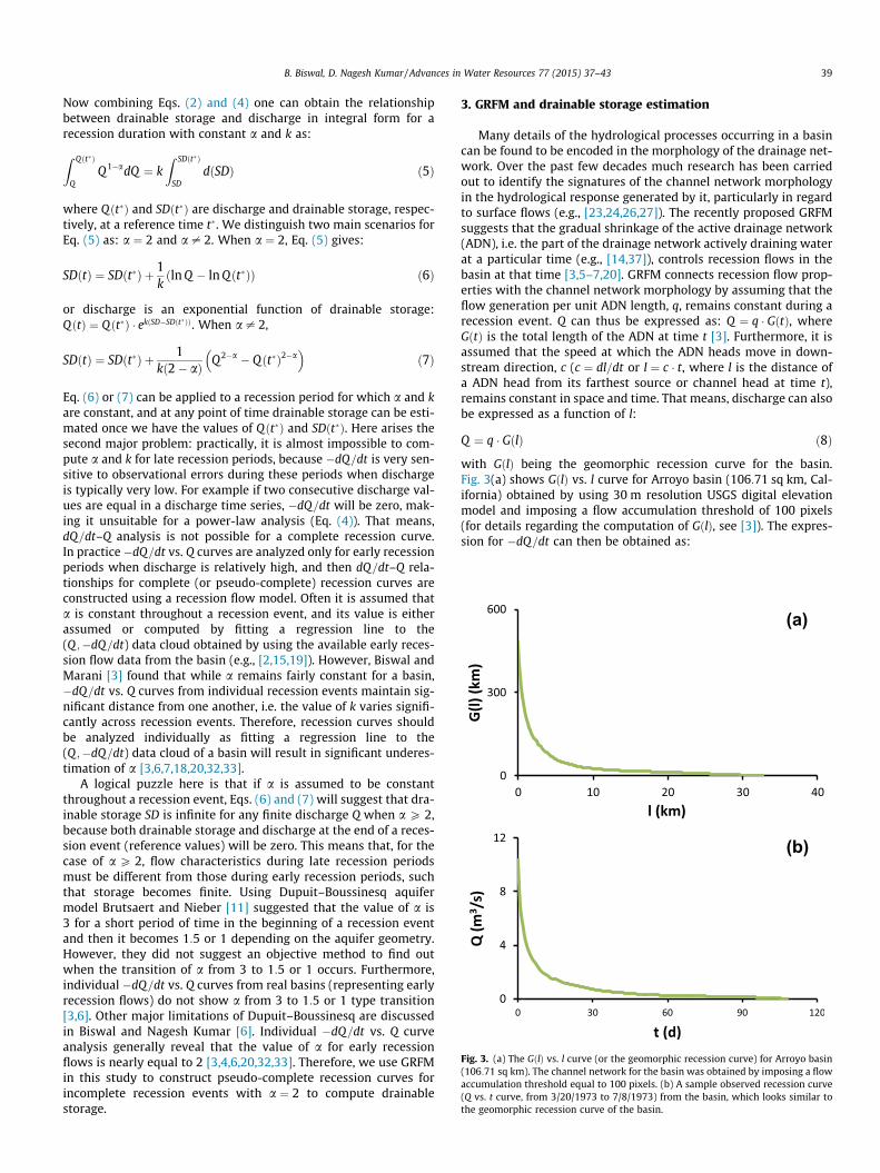
Fig. 3. (a) The GðlÞ vs. l curve (or the geomorphic recession curve) for Arroyo basin(106:71 sq km). The channel network for the basin was obtained by imposing a flowaccumulation threshold equal to 100 pixels. (b) A sample observed recession curve(Q vs. t curve, from 3/20/1973 to 7/8/1973) from the basin, which looks similar tothe geomorphic recession curve of the basin.

B. Biswal, D. Nagesh Kumar / Advances in Water Resources 77 (2015) 37–43 39

Now combining Eqs. (2) and (4) one can obtain the relationshipbetween drainable storage and discharge in integral form for arecession duration with constant a and k as:

Z Qðt�Þ

QQ 1�adQ ¼ k

Z SDðt�Þ

SDdðSDÞ ð5Þ

where Qðt�Þ and SDðt�Þ are discharge and drainable storage, respec-tively, at a reference time t�. We distinguish two main scenarios forEq. (5) as: a ¼ 2 and a – 2. When a ¼ 2, Eq. (5) gives:

SDðtÞ ¼ SDðt�Þ þ 1k

ln Q � ln Qðt�Þð Þ ð6Þ

or discharge is an exponential function of drainable storage:QðtÞ ¼ Qðt�Þ � ekðSD�SDðt�ÞÞ. When a – 2,

SDðtÞ ¼ SDðt�Þ þ 1kð2� aÞ Q 2�a � Qðt�Þ2�a

� �ð7Þ

Eq. (6) or (7) can be applied to a recession period for which a and kare constant, and at any point of time drainable storage can be esti-mated once we have the values of Qðt�Þ and SDðt�Þ. Here arises thesecond major problem: practically, it is almost impossible to com-pute a and k for late recession periods, because �dQ=dt is very sen-sitive to observational errors during these periods when dischargeis typically very low. For example if two consecutive discharge val-ues are equal in a discharge time series, �dQ=dt will be zero, mak-ing it unsuitable for a power-law analysis (Eq. (4)). That means,dQ=dt–Q analysis is not possible for a complete recession curve.In practice �dQ=dt vs. Q curves are analyzed only for early recessionperiods when discharge is relatively high, and then dQ=dt–Q rela-tionships for complete (or pseudo-complete) recession curves areconstructed using a recession flow model. Often it is assumed thata is constant throughout a recession event, and its value is eitherassumed or computed by fitting a regression line to the(Q ;�dQ=dt) data cloud obtained by using the available early reces-sion flow data from the basin (e.g., [2,15,19]). However, Biswal andMarani [3] found that while a remains fairly constant for a basin,�dQ=dt vs. Q curves from individual recession events maintain sig-nificant distance from one another, i.e. the value of k varies signifi-cantly across recession events. Therefore, recession curves shouldbe analyzed individually as fitting a regression line to the(Q ;�dQ=dt) data cloud of a basin will result in significant underes-timation of a [3,6,7,18,20,32,33].

A logical puzzle here is that if a is assumed to be constantthroughout a recession event, Eqs. (6) and (7) will suggest that dra-inable storage SD is infinite for any finite discharge Q when a P 2,because both drainable storage and discharge at the end of a reces-sion event (reference values) will be zero. This means that, for thecase of a P 2, flow characteristics during late recession periodsmust be different from those during early recession periods, suchthat storage becomes finite. Using Dupuit–Boussinesq aquifermodel Brutsaert and Nieber [11] suggested that the value of a is3 for a short period of time in the beginning of a recession eventand then it becomes 1:5 or 1 depending on the aquifer geometry.However, they did not suggest an objective method to find outwhen the transition of a from 3 to 1:5 or 1 occurs. Furthermore,individual �dQ=dt vs. Q curves from real basins (representing earlyrecession flows) do not show a from 3 to 1:5 or 1 type transition[3,6]. Other major limitations of Dupuit–Boussinesq are discussedin Biswal and Nagesh Kumar [6]. Individual �dQ=dt vs. Q curveanalysis generally reveal that the value of a for early recessionflows is nearly equal to 2 [3,4,6,20,32,33]. Therefore, we use GRFMin this study to construct pseudo-complete recession curves forincomplete recession events with a ¼ 2 to compute drainablestorage.

3. GRFM and drainable storage estimation

Many details of the hydrological processes occurring in a basincan be found to be encoded in the morphology of the drainage net-work. Over the past few decades much research has been carriedout to identify the signatures of the channel network morphologyin the hydrological response generated by it, particularly in regardto surface flows (e.g., [23,24,26,27]). The recently proposed GRFMsuggests that the gradual shrinkage of the active drainage network(ADN), i.e. the part of the drainage network actively draining waterat a particular time (e.g., [14,37]), controls recession flows in thebasin at that time [3,5–7,20]. GRFM connects recession flow prop-erties with the channel network morphology by assuming that theflow generation per unit ADN length, q, remains constant during arecession event. Q can thus be expressed as: Q ¼ q � GðtÞ, whereGðtÞ is the total length of the ADN at time t [3]. Furthermore, it isassumed that the speed at which the ADN heads move in down-stream direction, c (c ¼ dl=dt or l ¼ c � t, where l is the distance ofa ADN head from its farthest source or channel head at time t),remains constant in space and time. That means, discharge can alsobe expressed as a function of l:

Q ¼ q � GðlÞ ð8Þ

with GðlÞ being the geomorphic recession curve for the basin.Fig. 3(a) shows GðlÞ vs. l curve for Arroyo basin (106:71 sq km, Cal-ifornia) obtained by using 30 m resolution USGS digital elevationmodel and imposing a flow accumulation threshold of 100 pixels(for details regarding the computation of GðlÞ, see [3]). The expres-sion for �dQ=dt can then be obtained as:

(a)

(b)

Fig. 4. (a) NðlÞ vs. GðlÞ curve for Arroyo basin (106:71 sq km), which displays twodistinct scaling regimes: AB that corresponds to early recession flows (a ¼ 2) andBC that corresponds to late recession flows (a ¼ 0). The channel network for thebasin was obtained by imposing a flow accumulation threshold equal to 100 pixels.(b) AB part of an observed recession curve (lasting from 3/20/1973 to 7/8/1973)from the basin displaying �dQ=dt vs. Q power law relationship with power lawexponent nearly equal to 2. Note that BC parts of observed recession curves aregenerally dominated by significant errors (Red lines indicate slopes in the log–logplanes.). (For interpretation of the references to color in this figure legend, thereader is referred to the web version of this article.)

(a)

(b)

Fig. 5. (a) The KðlÞ vs. GðlÞ curve or the geomorphic storage–discharge curve ofArroyo basin (106:71 sq km) and (b) a selected observed recession curve from thebasin (from 3/20/1973 to 7/8/1973) displaying two distinct scaling relationships insemi logarithmic planes: exponential relationship for the regime AB and power lawrelationship for the regime BC (not clearly visible here).

40 B. Biswal, D. Nagesh Kumar / Advances in Water Resources 77 (2015) 37–43

� dQdt¼ �q � dl

dt� dGðlÞ

dl¼ q � c � NðlÞ ð9Þ

where NðlÞ is the number of ADN heads at distance l or time t. UsingEqs. (8) and (9), the expression for the geomorphic counterpart of�dQ=dt vs. Q curve (Eq. (4)) can be obtained as [3]:

NðlÞ ¼ q � GðlÞa ð10Þ

where q ¼ kqa�1=c.

The NðlÞ vs. GðlÞ curve of a basin typically displays two scalingregimes, AB and BC, easily distinguishable from one another ([3],also see Fig. 4(a)). The regime AB corresponds to early recessionflows, and for most basins the geomorphic a for this phase is alsonearly equal to 2, i.e. both geomorphic a and observed a are nearlyequal to 2 for the regime AB [3,6], suggesting that the model is ableto capture key details of a recession flow curve. Defining the geo-morphic storage KðlÞ as �dðKðlÞÞ=dl ¼ GðlÞ, the expression for thegeomorphic storage–discharge relationship in integral form fora ¼ 2 can be obtained by using Eq. (10):Z Gðl�Þ

GðlÞ

dGðlÞGðlÞ ¼ q

Z Kðl�Þ

KðlÞ� dKðlÞ ð11Þ

where l� ¼ c � t�, the reference distance. Now Eq. (11) produces thegeomorphic equivalent of drainable storage as:

KðlÞ ¼ Kðl�Þ þ 1q

ln GðlÞ � ln Gðl�Þð Þ ð12Þ

Eq. (12) suggests that the geomorphic storage–discharge relation-ship for part AB is exponential: GðlÞ ¼ Gðl�Þ � eqðKðlÞ�Kðl�ÞÞ. Fig. 5(a)

shows KðlÞ vs. GðlÞ curve for Arroyo basin displaying exponentialrelationship for its AB portion, with the transition point B being verynoticeable. Note that Eq. (6) can be easily retrieved fromEq. (12) using the relationships Q ¼ q � GðlÞ and SD ¼ �

RQdt ¼

�q �R

GðlÞ � dt=dl � dl ¼ q=c �KðlÞ. NðlÞ is always equal to 1 for thephase BC as only the mainstream of the channel network contrib-utes, which also means that a ¼ 0 for this phase (see Fig. 4(a)).GðlÞ for this phase is thus L� l, where L is the length of the main-stream of the channel network, and KðlÞ ¼ 1=2 � ðL� lÞ2. That means,

KðlÞ ¼ 12

GðlÞ2 ð13Þ

for the BC part of the recession curve. Fig. 6(a) separately shows BCportion of the KðlÞ vs. GðlÞ curve for Arroyo basin. Using the expres-sions for SD (SD ¼ q=c �KðlÞ, obtained from Eq. (2)) and Q(Q ¼ q � GðlÞ) it is found that drainable storage–discharge relation-ships for BC portions or late recession flows according to GRFMshould follow a power law relationship with exponent equal to 2:

SD / Q 2 ð14Þ

If the power law scaling transition (i.e. a changes from 2 to 0) takesplace at length l�, Eq. (10) suggests that Nðl�Þ ¼ 1 ¼ qGðl�Þ2 (i.e., BCphase starts at l� where Nðl�Þ is 1). We therefore find that ln GðlÞ�ln Gðl�Þ is lnðGðlÞ=Gðl�ÞÞ ¼ 1=2 � ln NðlÞ and Kðl�Þ is 1=2 � ðL� l�Þ2 ¼1=2 � Gðl�Þ2 ¼ 1=ð2qÞ. Thus, Eq. (12) can be expressed as:

KðlÞ ¼ 12qð1þ ln NðlÞÞ ð15Þ

According to Biswal and Marani [7], NðlÞ ¼ !ðlÞ � A for topologicallyrandom networks [31] when c is a constant. !ðlÞ is the constant ofproportionality and A is the basin area. We assume that the basinsselected here follow this criterion. Geomorphic storage KðlÞ canthus be written as:

(a)

(b)

Fig. 6. (a) The BC portion of the KðlÞ vs. GðlÞ curve of Arroyo basin (106:71 sq km) inlog–log plot displaying a power law relationship with exponent equal to 2(indicated by red line). (b) The BC portion of a selected observed recession curve(from 3/20/1973 to 7/8/1973) also displaying a power law relationship withexponent close to 2. (For interpretation of the references to color in this figurelegend, the reader is referred to the web version of this article.)

B. Biswal, D. Nagesh Kumar / Advances in Water Resources 77 (2015) 37–43 41

KðlÞ ¼ 12q

1þ ln Aþ wðlÞð Þ ð16Þ

where wðlÞ ¼ ln !ðlÞ. Recalling that storage SDðlÞ ¼ q=c �KðlÞ andk ¼ cq=q for a ¼ 2, the expression for drainable storage at any pointof time t can be obtained as

SDðtÞm ¼ SDðlÞm ¼ 12k

1þ ln Aþ wðlÞð Þ ð17Þ

The superscript m explicitly denotes that Eq. (17) gives modeleddrainable storage. Since wðlÞ is supposed to be constant acrossbasins, the variability of drainable storage SDðtÞ within a basin isrepresented by the variability of k only (17). It is interesting to notehere that Eq. (17) supports the earlier speculation that the dynamicparameter k is mainly controlled by the characteristic storage in thebasin [4,6,7,33].

In short, GRFM defines the shape of a recession curve. Thus, itcan be used to obtain a pseudo-complete recession curve for anincomplete recession event. As computation of k requires only afew early recession flow data points [3,6,32], Eq. (17) can be usedto estimate drainable storage for incomplete recession events oncewe have the value of the universal constant wðlÞ. However, the pre-dictability of Eq. (17) can be verified only when we have a com-plete recession curve, for which drainable storage can be directlyestimated using Eq. (3). In the next section we analyze completerecession curves from a number of basins compare observed drain-able storage (Eq. (17)) with modeled drainable storage (Eq. (3)).Note that even for a complete recession curve we use only earlyrecession flow data points (belonging to the AB part) to compute k.

4. Analysis of observed recession flow curves

We use daily average streamflow data and identify completerecession curves for 27 USGS basins that are relatively unaffected

by human activities (see Table S1 of the online supporting mate-rial). Theoretically, both Q and �dQ=dt should continuouslydecrease over time during a recession period. However, almostalways, this criterion is not satisfied due to errors (numericalerrors, measurement errors, etc.), particularly associated with laterecession flows (i.e. with the BC parts of recession curves). Here wevisually select relatively smooth looking recession curves startingfrom their respective peaks and lasting till discharge approachingzero (Fig. 3(b)). For convenience, we denote discharge in discreteform as Q z, the average discharge in the zth day during a recessionevent after the recession peak. For time t ¼ zþ 1=2 days, Q and�dQ=dt are computed by following Brutsaert and Nieber [11] as:Q ¼ ðQz þ Q zþ1Þ=2 and �dQ=dt ¼ ðQ z � Qzþ1Þ=Dt (here Dt is1 day). �dQ=dt often increases from t ¼ 1=2 day (z ¼ 0) toz ¼ 3=2 days (z ¼ 1), possibly because discharge during this periodis likely to be significantly controlled by storm flows, and then itkeeps on decreasing [3,6]. We thus discard the recession peakand compute drainable storage for z ¼ 1. Note that z ¼ 0 doesnot necessarily mean the beginning of a recession event. In fact,it is widely acknowledged that there is no objective definition forthe origin of a recession event (e.g., [11]). A recession curve is thenconsidered if at least 3 data points starting from z ¼ 1 (i.e. theybelong to the AB part, see Table S1) show a robust dQ=dt–Q powerlaw relationship (R2 > 0:7) with a ¼ 2� 0:25 (see, for e.g.,Fig. 4(b)). Note that BC phases of observational �dQ=dt vs. Q curvescannot be produced, even for the complete recession curves, as�dQ=dt is very sensitive to errors during late recession periods.In total, we select 121 complete recession curves from the 27basins for our analysis (see Table S1).

SDz, drainable storage in a basin in the zth day after the begin-ning of a complete recession event can be computed for a completerecession curve by discretizing Eq. (3) as:

SDoz ¼ Dt �

XZ

i¼z

Qi ð18Þ

where Z is the number of days for which the recession event lastsor the timescale of the recession curve (i.e. T ¼ Z days). The super-script o suggests that Eq. (18) deals with observed drainablestorage. The observed recession curves display drainable stor-age–discharge patterns very similar to those of the geomorphicrecession curves. The AB parts of observed recession curves dis-play exponential SD–Q relationship as predicted by Eq. (12) (seeFig. 5(b)). The BC parts exhibit power law SD–Q relationship withexponent nearly equal to 2 (see Fig. 6(b)), though not in all casesbecause of the dominance of errors during this phase. It should benoted here that the discontinuation of exponential SD–Q relation-ship was also reported in some past studies (e.g., [2,16]).However, none of those studies had investigated when and howthe discontinuation occurs and, more importantly, its physicalsignificance.

Now we focus our attention on evaluating the applicability ofEq. (17). Particularly, for each recession curve we obtain observedSD for z ¼ 1 (SDo

1) following Eq. (18). Then we follow least squarelinear regression method and compute k for each recession curveby fitting a line with slope a ¼ 2 to the selected early recession per-iod (Q ;�dQ=dt) data points (see Table S1) in the double logarith-mic plane [6,7]. Note that for modeling drainable storage forz ¼ 1 (SDm

1 ) using Eq. (17) the value of w needs to be determinedfrom recession flow data as we do not have information on the val-ues of NðlÞ and GðlÞ at z ¼ 1. Therefore, we compute the value of w1

(w for z ¼ 1) for each recession curve by putting SDo1 (computed by

using Eq. (18)) in Eq. (17). The mean value w1 obtained by consid-ering all the recession curves is found to be nearly equal to 1 (1:02),which gives the expression for SD1 as:

42 B. Biswal, D. Nagesh Kumar / Advances in Water Resources 77 (2015) 37–43

SDm1 ¼

1k

1þ 0:5 ln Að Þ ð19Þ

We thereafter use Eq. (19) to compute SDm1 for all the recession

curves (i.e. by considering that w1 ¼ 1 for all the recession curvesfrom all the basins). Fig. 7 shows the plot between SDm

1 and SDo1

for the selected recession curves with correlation R2 ¼ 0:96 andthe slope of SDm

1 vs. SDo1 line is 1:06, which is quite close to 1, indi-

cating that SDm1 � SDo

1 in general. Another convincing evidence isthat the condition w1 ¼ lnðN1=AÞ ¼ 1 (N1 being N1 at z ¼ 1), whichimplies that N1 ¼ e � A, is physically very plausible. According toShreve [31], for random networks A � 1=D2

1 � ð2N1 � 1), where D1 isthe active drainage density [7] at z ¼ 1. For real basins N1 is largeenough to consider that 2N1 � 1 � 2N1. Thus we obtainD1 ¼

ffiffiffiffiffiffiffiffiffi2 � ep

� 2:33 km�1, which is quite realistic (see, for e.g., [8]).These observations strongly suggest that the proposed model is quiterobust to predict drainable storage. Most importantly, Eq. (19) can beused to estimate drainable storage for incomplete recession events asit requires only the value of k, which can be computed by consideringa few days of early recession flow discharge data.

It should be noted that various errors and uncertainties mightaffect estimation of drainable storage with the use of Eq. (19).Errors associated with discharge measurements might affect thecomputation k. Spatial rainfall variation might also introduceerrors [4]. The value of w1 might vary across events and basins.Though Eq. (19) is valid for a ¼ 2, our analysis suggests computa-tion k by allowing some deviation for a, which might introducesome uncertainty. Thus, future studies need to estimate drainablestorage for scenarios when a shows large deviation from 2 as Eq.(19) is meant for scenarios when a is nearly equal to 2. Further-more, Eq. (19) is based on GRFM whose assumption that both qand c remain constant for a recession event might not be very accu-rate always. However, despite of all these limitations, the resultsobtained by using Eq. (19) seem to be promising. Potential implica-tions of the observations in this study, therefore, include moreaccurate prediction in ungauged basins for better management offresh water resources and ecosystems. The strong R2 correlationbetween SDm

1 and SDo1 may also be suggesting that the value of

w1 is universal, meaning that for a basin not considered in thisstudy SD1 can be estimated for any of its recession event by com-puting k from the early recession flow data and considering thatw1 ¼ 1. This aspect needs to be rigorously tested as our datasetincludes basins only from some selected parts of the US. Also notethat the present study uses data from relatively small and homoge-neous basins (drainage area ranging from 2:85 km2 to 595:70 km2)as it is not possible for us to obtain complete recession curves for

Fig. 7. Modeled drainable storage one day after the recession peak (SDm1 ) vs.

observed drainable storage one day after the recession peak (SDo1) for the 121

complete recession curves selected in this study. Good correlation (R2 ¼ 0:96)indicates that the predictions are reliable.

large basins (say the Mississippi river basin). Thus, further investi-gation is required to analyze drainable storage–discharge relation-ships of large river basins that can even witness spatial variation inclimate and geology (e.g., [30]). These objectives can possibly beachieved by introducing meaningful modifications to GRFM (e.g.,[5,20]) and then obtaining a more robust expression for drainablestorage.

5. Summary

The state of the art technologies do not enable us to instantlyestimate water stored within a drainage basin. Therefore, hydrolo-gists generally estimate storage by expressing it as a function ofbasin inflow and outflow components that are measurable. Ouraim in this study was to estimate only the part of basin storage thattransforms later into streamflows or ‘drainable’ storage. While it isstraightforward to estimate drainable storage when recessionevents are ‘complete’, the same cannot be done when recessionevents are ‘incomplete’ due to short inter-storm time intervals.One possible solution is to use a hydrological model to construct‘pseudo-complete’ recession curves from incomplete recessioncurves. Thus, it is essential to carefully analyze and model recessionflow curves. Brutsaert and Nieber [11] suggested to expresses timerate of change of discharge (dQ=dt) as a function of Q, which com-monly takes the form: �dQ=dt ¼ kQa. However, the problem is thatdQ=dt–Q analysis is not practically possible for late recession peri-ods when discharge is relatively low. Studies dealing with recessionflows often consider early discharge observations for a recessionevent to compute a and assume that its value is constant for thewhole recession period. Interestingly, a for early recession flowsfrom natural basins is generally close to 2, in which case the con-stant a assumption suggests that storage is infinite for any finite dis-charge. That means a for late recession flows must be different fromthat of early recession flows. We addressed this issue in this studyusing geomorphological recession flow model (GRFM).

GRFM suggests that a �dQ=dt vs. Q curve exhibits two distinctscaling regimes: AB, which corresponds to early recession flows,and BC, which corresponds to late recession flows. While theregime AB gives a � 2;a for the regime BC is 0 according to themodel. That means drainable storage–discharge relationshipaccording to GRFM is exponential for AB regimes and power lawwith exponent equal to 2 for BC regimes. The transition thus makesdrainable storage finite. Using data from 27 basins we found thatthe observed recession curves, like the modeled (geomorphic)recession curves, indeed display exponential discharge-storagerelationship for AB parts and power law relationships for BC parts.We then followed suitable analytical methods and obtained a sim-plified expression for drainable storage one day after a recessionpeak (SD1) as a function of k and basin area: SD1 ¼ 1=k 1þð0:5 ln AÞ. We observed that SDm

1 matches well with SDo1 (R2 ¼ 0:96

and the slope of the linear regression line being 1:06). Despitemany critical assumptions in the model formulation, the observa-tions in this study are quite encouraging. Another interestingobservation is that according to our model the active drainage den-sity one day after a recession peak (D1) should be approximatelyequal to 2:33 km�1, which is quite realistic. Results in this study,therefore, are suggestive of the possibility that the proposed modelcan be used to estimate drainable storage for various importantpurposes related to water resources management, particularlywhen the recession events are incomplete.

Acknowledgments

The authors are thankful to the three anonymous reviewers fortheir insightful comments and suggestions.

B. Biswal, D. Nagesh Kumar / Advances in Water Resources 77 (2015) 37–43 43

Appendix A. Supplementary data

Supplementary data associated with this article can be found, inthe online version, at http://dx.doi.org/10.1016/j.advwatres.2014.12.009.

References

[1] Alsdorf DE, Lettenmaier DP. Tracking fresh water from space. Science2003;301:1492–4. http://dx.doi.org/10.1126/science.1089802.

[2] Beven KJ, Kirkby MJ. A physically based variable contributing area model ofbasin hydrology. Hydrol Sci Bull 1979;24(1):43–69. http://dx.doi.org/10.1080/02626667909491834.

[3] Biswal B, Marani M. Geomorphological origin of recession curves. Geophys ResLett 2010;37:L24403. http://dx.doi.org/10.1029/2010GL045415.

[4] Biswal B, Nagesh Kumar D. Study of dynamic behaviour of recession curves.Hydrol Process 2014;28:784–92. http://dx.doi.org/10.1002/hyp.9604.

[5] Biswal B, Nagesh Kumar D. A general geomorphological recession flow modelfor river basins. Water Resour Res 2013. http://dx.doi.org/10.1002/wrcr.20379.

[6] Biswal B, Nagesh Kumar D. What mainly controls recession flows in riverbasins? Adv Water Resour 2014;65:25–33. http://dx.doi.org/10.1016/j.advwatres.2014.01.001.

[7] Biswal B, Marani M. ‘Universal’ recession curves and their geomorphologicalinterpretation. Adv Water Resour 2014;65:34–42. http://dx.doi.org/10.1016/j.advwatres.2014.01.004.

[8] Blyth K, Rodda JC. A stream length study. Water Resour Res1973;9(5):1454–61. http://dx.doi.org/10.1029/WR009i005p01454.

[9] Botter G, Porporato A, Rodriguez-Iturbe I, Rinaldo A. Nonlinear storage–discharge relations and catchment streamflow regimes. Water Resour Res2009;45:W10427. http://dx.doi.org/10.1029/2008WR007658.

[10] Botter G, Basso S, Rodriguez-Iturbec I, Rinaldo A. Resilience of river flowregimes. Proc Natl Acad Sci USA 2014;110(32):12925–30. http://dx.doi.org/10.1073/pnas.1311920110.

[11] Brutsaert W, Nieber JL. Regionalized drought flow hydrographs from a matureglaciated plateau. Water Resour Res 1977;13(3):637–44. http://dx.doi.org/10.1029/WR013i003p00637.

[12] Brutsaert W, Lopez JP. Basin-scale geohydrologic drought flow features ofriparian aquifers in the southern great plains. Water Resour Res1998;34:233–40. http://dx.doi.org/10.1029/97WR03068.

[13] Delworth TL, Manabe S. Climate variability and land-surface processes. AdvWater Resour 1993;16:3–20. http://dx.doi.org/10.1016/0309-1708(93)90026-C.

[14] Gregory KJ, Walling DE. The variation of drainage density within a catchment.Bull Int Assoc Sci Hydrol 1968;13(2):61–8. http://dx.doi.org/10.1080/02626666809493583.

[15] Kirchner JW. Catchments as simple dynamical systems: catchmentcharacterization, rainfall–runoff modeling, and doing hydrology backwards.Water Resour Res 2009;45:W02429. http://dx.doi.org/10.1029/2008WR006912.

[16] Lambert AO. Catchment models based on ISO functions. J Inst Water Eng1972;26(8):413–22.

[17] Marani M, Eltahir E, Rinaldo A. Geomorphic controls on regional baseflow.Water Resour Res 2001;37(10):2619–30. http://dx.doi.org/10.1029/2000WR000119.

[18] McMillan H, Gueguen M, Grimon E, Woods R, Clark M, Clark M, Rupp DE.Spatial variability of hydrological processes and model structure diagnostics ina 50 km2 catchment. Hydrol Process 2013. http://dx.doi.org/10.1002/hyp.9988.

[19] Moore RJ. The PDM rainfall–runoff model. Hydrol Earth Syst Sci2007;11:483–99. http://dx.doi.org/10.5194/hess-11-483-2007.

[20] Mutzner R, Bertuzzo E, Tarolli P, Weijs SV, Nicotina L, Ceola S, Tomasic N,Rodriguez-Iturbe I, Parlange MB, Rinaldo A. Geomorphic signatures onBrutsaert base flow recession analysis. Water Resour Res 2013;49:5462–72.http://dx.doi.org/10.1002/wrcr.20417.

[21] Papa F, Guntner A, Frappart F, Prigent C, Rossow WB. Variations of surfacewater extent and water storage in large river basins: a comparison of differentglobal data sources. Geophys Res Lett 2008;35:L11401. http://dx.doi.org/10.1029/2008GL033857.

[22] Reager JT, Famiglietti JS. Characteristic mega-basin water storage behaviorusing GRACE. Water Resour Res 2013;49:3314–29. http://dx.doi.org/10.1002/wrcr.20264.

[23] Rigon R, D’Odorico P, Bertoldi G. The geomorphic structure of the runoff peak.Hydrol Earth Syst Sci 2011;2011(15):1853–63. http://dx.doi.org/10.5194/hess-15-1853-2011.

[24] Rinaldo A, Botter G, Bertuzzo E, Uccelli A, Settin T, Marani M. Transport atbasin scales: 1. Theoretical framework. Hydrol Earth Syst Sci 2006;10:19–29.http://dx.doi.org/10.5194/hess-10-19-2006.

[25] Rinaldo A, Rigon R, Banavar JR, Maritan A, Rodriguez-Iturbe I. Evolution andselection of river networks: statics, dynamics, and complexity. Proc Natl AcadSci USA 2014;111(11):3900–2. http://dx.doi.org/10.1073/pnas.1322700111.

[26] Rodriguez-Iturbe I, Valdes JB. The geomorphologic structure of the hydrologicresponse. Water Resour Res 1979;15(6):1409–20. http://dx.doi.org/10.1029/WR015i006p01409.

[27] Rodrguez-Iturbe I, Rinaldo A. Fractal river basins: chance and selforganization. New York: Cambridge Univ Press; 1997.

[28] Rodriguez-Iturbe I, Muneepeerakul R, Bertuzzo E, Levin SA, Rinaldo A. Rivernetworks as ecological corridors: a complex systems perspective forintegrating hydrologic, geomorphologic, and ecologic dynamics. WaterResour Res 2009;45:W01413. http://dx.doi.org/10.1029/2008WR007124.

[29] Rupp DE, Woods RA. Increased flexibility in base flow modelling using a powerlaw transmissivity profile. Hydrol Process 2008;22:2667–71. http://dx.doi.org/10.1002/hyp.6863.

[30] Schaller MF, Fan Y. River basins as groundwater exporters and importers:implications for water cycle and climate modeling. J Geophys Res2009;114:D04103. http://dx.doi.org/10.1029/2008JD010636.

[31] Shreve R. Infinite topologically random channel networks. J Geol1967;75(2):178–86. http://dx.doi.org/10.1086/627245.

[32] Shaw SB, Riha SJ. Examining individual recession events instead of a datacloud: using a modified interpretation of dQ=dt-Q streamflow recession inglaciated watersheds to better inform models of low flow. J Hydrol 2012;434–435:46–54. http://dx.doi.org/10.1016/j.jhydrol.2012.02.034.

[33] Shaw SB, McHardy TM, Riha SJ. Evaluating the influence of watershed moisturestorage on variations in base flow recession rates during prolonged rain-freeperiods in medium-sized catchments in New York and Illinois, USA. WaterResour Res 2013;49:6022–8. http://dx.doi.org/10.1002/wrcr.20507.

[34] Stoelzle M, Stahl K, Weiler M. Are streamflow recession characteristics reallycharacteristic? Hydrol Earth Syst Sci 2013;17:817–28. http://dx.doi.org/10.5194/hess-17-817-2013.

[35] Troch PA, De Troch FP, Brutsaert W. Effective water table depth to describeinitial conditions prior to storm rainfall in humid regions. Water Resour Res1993;29:427–34. http://dx.doi.org/10.1029/92WR02087.

[36] Troch PA et al. The importance of hydraulic groundwater theory in catchmenthydrology: the legacy of Wilfried Brutsaert and Jean-Yves Parlange. WaterResour Res 2013;49:5099–116. http://dx.doi.org/10.1002/wrcr.20407.

[37] Weyman DR. Throughflow in hillslopes and its relation to stream hydrograph.Bull Int Assoc Sci Hydrol 1970;15(3):25–33. http://dx.doi.org/10.1080/02626667009493969.