Estimation in inverse problems and second-generation wavelets

Estimation in inverse problems and second-generationwavelets

Dominique Picard and Gérard Kerkyacharian

Abstract. We consider the problem of recovering a function f when we receive a blurred (by alinear operator) and noisy version: Yε = Kf + εW . We will have as guides 2 famous examplesof such inverse problems: the deconvolution and the Wicksell problem. The direct problem (Kis the identity) isolates the denoising operation. It cannot be solved unless accepting to estimatea smoothed version of f : for instance, if f has an expansion on a basis, this smoothing mightcorrespond to stopping the expansion at some stage m. Then a crucial problem lies in findingan equilibrium for m, considering the fact that for m large, the difference between f and itssmoothed version is small, whereas the random effect introduces an error which is increasingwithm. In the true inverse problem, in addition to denoising, we have to ‘inverse the operator’K ,an operation which not only creates the usual difficulties, but also introduces the necessity tocontrol the additional instability due to the inversion of the random noise. Our purpose here isto emphasize the fact that in such a problem there generally exists a basis which is fully adaptedto the problem, where for instance the inversion remains very stable: this is the singular valuedecomposition basis. On the other hand, the SVD basis might be difficult to determine andto numerically manipulate. It also might not be appropriate for the accurate description of thesolution with a small number of parameters. Moreover, in many practical situations the signalprovides inhomogeneous regularity, and its local features are especially interesting to recover.In such cases, other bases (in particular, localised bases such as wavelet bases) may be muchmore appropriate to give a good representation of the object at hand. Our approach here willbe to produce estimation procedures keeping the advantages of a localisation properly withoutloosing the stability and computability of SVD decompositions. We will especially considertwo cases. In the first one (which is the case of the deconvolution example) we show that afairly simple algorithm (WAVE-VD), using an appropriate thresholding technique performed ona standard wavelet system, enables us to estimate the object with rates which are almost optimalup to logarithmic factors for any Lp loss function and on the whole range of Besov spaces. Inthe second case (which is the case of the Wicksell example where the SVD basis lies in therange of Jacobi polynomials) we prove that a similar algorithm (NEED-VD) can be performedprovided one replaces the standard wavelet system by a second generation wavelet-type basis:the needlets. We use here the construction (essentially following the work of Petrushev andco-authors) of a localised frame linked with a prescribed basis (here Jacobi polynomials) usinga Littlewood–Paley decomposition combined with a cubature formula. Section 5 describes thedirect case (K = I ). It has its own interest and will act as a guide for understanding the ‘true’inverse models for a reader who is not familiar with nonparametric statistical estimation. It canbe read first. Section 1 introduces the general inverse problem and describes the examples ofdeconvolution and Wicksell’s problem. A review of standard methods is given with a specialfocus on SVD methods. Section 2 describes the WAVE-VD procedure. Section 3 and 4 give adescription of the needlets constructions and the performances of the NEED-VD procedure.

Mathematics Subject Classification (2000). 62G07, 62G20, 62C20.

Keywords. Nonparametric estimation, denoising, inverse models, thresholding, Meyer wavelet,singular value decomposition, Littlewood–Paley decomposition.

Proceedings of the International Congressof Mathematicians, Madrid, Spain, 2006© 2006 European Mathematical Society

714 Dominique Picard and Gérard Kerkyacharian

1. Inverse models

Let H and K be two Hilbert spaces. K is a linear operator: f ∈ H �→ Kf ∈ K. Thestandard linear ill-posed inverse problem consists of recovering a good approximationfε of f , solution of

g = Kf, (1)

when only a perturbation gε of g is observed. In this paper we will consider the casewhere this perturbation is an additive stochastic white noise. Namely, we observe Yεdefined by the following equation:

Yε = Kf + εW, H, K, (2)

where ε is the amplitude of the noise. It is supposed to be a small parameter whichwill tend to 0. Our error will be measured in terms of this small parameter.

W is a K-white noise: i.e. for any g, h in K, ξ(g) := (W, g)K, ξ(h) := (W, h)Kform a random gaussian vector, centered, with marginal variance ‖g‖2

K, ‖h‖2

K, and

covariance (g, h)K (with the obvious extension when one considers k functions insteadof 2).

Equation (2) means that for any g in K, we observe Yε(g) := (Yε, g)K =(Kf, g)K + εξ(g) where ξ(g) ∼ N(0, ‖g‖2), and Yε(g), Yε(h) are independentrandom variables for orthogonal functions g and h.

The case whereK is the identity is called the ‘direct model’ and is summarized asa memento in Section 5. The reader who is unfamiliar with nonparametric statisticalestimation is invited to consult this section, which will act as a guide for understandingthe more general inverse models. In particular it is recalled therein that the model(2) is in fact an approximation of models appearing in real practical situations, forinstance the case where (2) is replaced by a discretisation.

1.1. Two examples: the problem of deconvolution and Wicksell’s problem

1.1.1. Deconvolution. The following problem is probably one of the most famousamong inverse problems in signal processing. In the deconvolution problem weconsider the following operator. In this case let H = K be the set of square integrableperiodic functions with the standard L2([0, 1]) norm and consider

f ∈ H �→ Kf =∫ 1

0γ (u− t)f (t) dt ∈ H, (3)

where γ is a known function of H, which is generally assumed to be a regular function(often in the sense that its Fourier coefficients γk behave like k−ν). A very commonexample is also the box-car function: γ (t) = 1

2a I{[−a, a]}(k).The following figures show first four original signals to recover, which are well-

known test-signals of the statistical literature. They provide typical features which aredifficult to restore: bumps, blocks and Doppler effects. The second and third series of

Estimation in inverse problems and second-generation wavelets 715

pictures show their deformation after blurring (i.e. convolution with a regular function)and addition of a noise. These figures show how the convolution regularizes the signal,making it very difficult to recover, especially the high frequency features. A statisticalinvestigation of these signals can be found in [22].

A variant of this problem consists in observing Y1, . . . , Yn, n independent andidentically distributed random variables where eachYi may be written asYi = Xi+Ui ,whereXi andUi again are independent, the distribution ofUi is known and of densityγand we want to recover the common density of the Xi’s. The direct problem is thecase where Ui = 0, for all i, and is corresponding to a standard density estimationproblem (see Section 5.1) . Hence the variables Ui are acting as perturbations of theXi’s, whose density is to be recovered.

0 0.2 0.4 0.6 0.8 1 0. 5

0

0.5

1

1.5

2

2.5(a) Lidar

0 0.2 0.4 0.6 0.8 10

1

2

3

4

5

6(b) Bumps

0 0.2 0.4 0.6 0.8 1 0.5

0

0.5

1

1.5(c) Blocks

0 0.2 0.4 0.6 0.8 1 0.5

0

0.5(d) Doppler

__

_

0 0.2 0.4 0.6 0.8 10

0.5

1

1.5

2

2.5(a) Blurred LIDAR

0 0.2 0.4 0.6 0.8 1 0.5

0

0.5

1

1.5(b) Blurred Bumps

0 0.2 0.4 0.6 0.8 1 0.5

0

0.5

1

1.5(c) Blurred Blocks

0 0.2 0.4 0.6 0.8 1 0.5

0

0.5(d) Blurred Doppler

_

_

_

0 0.2 0.4 0.6 0.8 1 0. 5

0

0.5

1

1.5

2

2.5(a) Noisyblurred LIDAR

0 0.2 0.4 0.6 0.8 1 0.5

0

0.5

1

1.5(b) Noisyblurred Bumps

0 0.2 0.4 0.6 0.8 1 0.5

0

0.5

1

1.5(c) Noisyblurred Blocks

0 0.2 0.4 0.6 0.8 1 0.8

0.6

0.4

0.2

0

0.2

0.4

0.6(d) Noisyblurred Doppler

_

_

_

_

_

_

_

1.1.2. Wicksell’s problem. Another typical example is the following classicalWick-sell problem [42]. Suppose a population of spheres is embedded in a medium. Thespheres have radii that may be assumed to be drawn independently from a density f .A random plane slice is taken through the medium and those spheres that are inter-sected by the plane furnish circles the radii of which are the points of observationY1, . . . , Yn. The unfolding problem is then to infer the density of the sphere radiifrom the observed circle radii. This unfolding problem also arises in medicine, where


the spheres might be tumors in an animal’s liver [36], as well as in numerous othercontexts (biological, engineering,…), see for instance [9].

Following [42] and [23], Wicksell’s problem corresponds to the following opera-tor:

H = L2([0, 1], dμ) dμ(x) = (4x)−1dx,

K = L2([0, 1], dλ) dλ(x) = 4π−1(1 − y2)1/2dy

Kf (y) = π

4y(1 − y2)−1/2

∫ 1

y

(x2 − y2)−1/2f (x)dμ.

Notice, however, that in this presentation, again in order to avoid additional tech-nicalities, we handle this problem in the white noise framework, which is simplerthan the original problem expressed above in density terms.

1.2. Singular value decomposition and projection methods. Let us begin with aquick description of well-known methods in inverse problems with random noise.

Under the assumption that K is compact, there exist 2 orthonormal bases (SVDbases) (ek) of H and (gk) of K, respectively, and a sequence (bk), tending to 0 when kgoes to infinity, such that

Kek = bkgk, K∗gk = bkek

if K∗ is the adjoint operator.For the sake of simplicity we suppose in the sequel that K and K∗ are into.

Otherwise we have to take care of the kernels of these operators. The bases (ek)and (gk) are called singular value bases, whereas the bk’s are simply called singularvalues.

Deconvolution. In this standard case simple calculations prove that the SVD bases(ek) and (gk) both coincide with the Fourier basis. The singular values are corre-sponding to the Fourier coefficients of the function γ :

bk = γk. (4)

Wicksell. In this case, following [23], we have the following SVD:

ek(x) = 4(k + 1)1/2x2P0,1k (2x2 − 1),

gk(y) = U2k+1(y).

P0,1k is the Jacobi polynomial of type (0, 1) with degree k, and Uk is the second type

Chebyshev polynomial with degree k. The singular values are

bk = π

16(1 + k)−1/2. (5)


1.2.1. SVD method. The singular value decomposition (SVD) of K ,

Kf =∑k

bk〈f, ek〉gk,

gives rise to approximations of the type

fε =N∑k=0

b−1k 〈yε, gk〉ek,

where N = N(ε) has to be chosen properly. This SVD method is very attractivetheoretically and can be shown to be asymptotically optimal in many situations (seeMathé and Pereverzev [31], Cavalier and Tsybakov [6], Mair and Ruymgaart [29]). Italso has the big advantage of performing a quick and stable inversion of the operator.However, it suffers from different types of limitations. The SVD bases might bedifficult to determine as well as to numerically manipulate. Secondly, while thesebases are fully adapted to describe the operator K , they might not be appropriate forthe accurate description of the solution with a small number of parameters.

Also in many practical situations the signal provides inhomogeneous regularity,and its local features are especially interesting to recover. In such cases other bases(in particular localised bases such as wavelet bases) may be much more appropriateto give a good representation of the object at hand.

1.2.2. Projection methods. Projection methods which are defined as solutions of(1) restricted to finite dimensional subspaces HN and KN (of dimension N) also giverise to attractive approximations of f , by properly choosing the subspaces and thetuning parameterN (Dicken and Maass [10], Mathé and Pereverzev [31] together withtheir non linear counterparts Cavalier and Tsybakov [6], Cavalier et al. [7], Tsybakov[41], Goldenshluger and Pereverzev [19], Efromovich and Koltchinskii [16]). In thecase where H = K and K is a self-adjoint operator, the system is particularly simpleto solve since the restricted operatorKN is symmetric positive definite. This is the so-called Galerkin method. Obviously, restricting to finite subspaces has similar effectsand can also be seen as a Tychonov regularisation, i.e. minimizing the least squarefunctional penalised by a regularisation term.

The advantage of the Galerkin method is to allow the choice of the basis. Howeverthe Galerkin method suffers from the drawback of being unstable in many cases.

Comparing the SVD and Galerkin methods exactly states one main difficulty ofthe problem. The possible antagonism between the SVD basis where the inversionof the system is easy, and a ‘localised’ basis where the signal is sparsely represented,will be the issue we are trying to address here.

1.3. Cut-off, linear methods, thresholding. The reader may profitably look at Sub-sections 5.3 and 5.4, where the linear methods and thresholding techniques are pre-sented in detail in the direct case.


SVD as well as Galerkin methods are very sensitive with respect to the choice ofthe tuning parameter N(ε). This problem can be solved theoretically. However thesolution heavily depends on prior assumptions of regularity on the solution, whichhave to be known in advance.

In the last ten years, many nonlinear methods have been developed especially inthe direct case with the objective of automatically adapting to the unknown smooth-ness and local singular behavior of the solution. In the direct case, one of the mostattractive methods is probably wavelet thresholding, since it allies numerical simplic-ity to asymptotic optimality on a large variety of functional classes such as Besov orSobolev classes.

To adapt this approach in inverse problems, Donoho [11] introduced a wavelet-likedecomposition, specifically adapted to the operator K (wavelet–vaguelette-decom-position) and provided a thresholding algorithm on this decomposition. In Abramo-vitch and Silverman [1], this method was compared with the similar vaguelette–wavelet-decomposition. Other wavelet approaches, might be mentioned such as An-toniadis and Bigot [2], Antoniadis et al. [3] and, especially for the deconvolutionproblem, Penski and Vidakovic [37], Fan and Koo [17], Kalifa and Mallat [24], Nee-lamani et al. [34].

Later, Cohen et al. [8] introduced an algorithm combining a Galerkin inversionwith a thresholding algorithm.

The approach developed in the sequel is greatly influenced by these previousworks. The accent we put here is on constructing (when necessary) new generationwavelet-type bases well adapted to the operatorK , instead of sticking to the standardwavelet bases and reducing the range of potential operators covered by the method.

2. Wave-VD-type estimation

We explain here the basic idea of the method, which is very simple. Let us expand fusing a well-suited basis (‘the wavelet-type’ basis’, to be defined later):

f =∑

(f, ψλ)Hψλ.

Using Parseval’s identity we have βλ = (f, ψλ)H = ∑fiψ

iλ for fi = (f, ei)H and

ψiλ = (ψλ, ei)H. Let us put Yi = (Yε, gi)K. We then have

Yi = (Kf, gi)K +εξi = (f,K∗gi)K +εξi =( ∑

j

fj ej ,K∗gi

)H

+εξi = bifi+εξi,

where the ξi’s are forming a sequence of independent centered gaussian variables withvariance 1. Furthermore,

βλ =∑i

Yi

biψiλ


is such that E(βλ) = βλ (i.e. its average value is βλ). It is a plausible estimate of βλ.Let us now put ourselves in a multiresolution setting, taking λ = (j, k) for j ≥ 0, kbelonging to a set χj , and consider

f =J∑

j=−1

∑k∈χj

t (βjk)ψjk,

where t is a thresholding operator. (The reader who is unfamiliar with thresholdingtechniques is referred to Section 5.4.)

t (βjk) = βjkI {|βjk| ≥ κtεσj }, tε = ε√

log 1/ε, (6)

where I {A} denotes the indicator function of the setA∗. Here κ is a tuning parameterof the method which will be properly chosen later. A main difference here with thedirect case is the fact that the thresholding is depending on the resolution level throughthe constant σj which also will be stated more precisely later. Our main discussionwill concern the choice of the basis (ψjk). In particular, we shall see that coherenceproperties with the SVD basis are of special interest.

We will particularly focus on two situations (corresponding to the two examplesdiscussed in the introduction). In the first type of cases, the operator has as SVD basesthe Fourier basis. In this case, this ‘coherence’ is easily obtained with ‘standard’wavelets (still, not any kind of standard wavelet as will be seen). However, moredifficult problems (and typically Wicksell’s problem) require, when we need to mixthese coherence conditions with the desired property of localisation of the basis, theconstruction of new objects: second generation-type wavelets.

2.1. WAVE-VD in a wavelet scenario. In this section we take {ψjk, j ≥ −1,k ∈ χj } to be a standard wavelet basis. More precisely, we suppose as usual thatψ−1 stands for the scaling function and, for any j ≥ −1, χj is a set of order 2j

contained in N. Moreover, we assume that the following properties are true. Thereexist constants cp, Cp, dp such that

cp2j (p2 −1) ≤ ‖ψjk‖pp ≤ Cp2j (

p2 −1), (7)∥∥∥ ∑

k∈χjukψjk

∥∥∥pp

≤ Dp∑k∈χj

|upk |‖ψjk‖pp for any sequence uk. (8)

It is well known (see for instance Meyer [32]) that wavelet bases provide charac-terisations of smoothness spaces such as Hölder spaces Lip(s), Sobolev spaces Ws

p

as well as Besov spaces Bspq for a range of indices s depending on the wavelet ψ .For the scale of Besov spaces which includes as particular cases Lip(s) = Bs∞∞ (ifs ∈ N) and Ws

p = Bspp (if p = 2), the characterisation has the following form:

If f =∑j≥−1

∑k∈Z

βjkψjk, then ‖f ‖Bspq ∼ ∥∥(2j [s+

12 − 1

p]‖βj ·‖lp

)j≥−1

∥∥lq. (9)


As in Section 5, we consider the loss of a decision f if the truth is f as the Lp

norm ‖f − f ‖p, and its associated risk

E‖f − f ‖pp .Here E denotes the expectation with respect to the random part of the observation yε.The following theorem is going to evaluate this risk, when the strategy is the oneintroduced in the previous section, and when the true function belongs to a Besov ball(f ∈ Bsπ,r (M) ⇐⇒ ‖f ‖Bspq ≤ M). One nice property of this estimation procedureis that it does not need the a priori knowledge of this regularity to get a good rate ofconvergence. If (ek) is the SVD basis introduced in Section 1.2, bk are the singularvalues and ψijk = 〈ei, ψjk〉, we consider the estimator f defined in the beginning ofSection 2.

Theorem 2.1. Assume that 1 < p < ∞, 2ν + 1 > 0 and

σ 2j :=

∑i

[ψijk

bi

]2

≤ C22jν for all j ≥ 0. (10)

Put κ2 ≥ 16p, 2J = [tε] −22ν+1 . If f belongs to Bsπ,r (M) with π ≥ 1, s ≥ 1/π , r ≥ 1

(with the restriction r ≤ π if s = (2ν + 1)( p

2π − 12

)), then we have

E‖f − f ‖pp ≤ C log(1/ε)p−1[ε2 log(1/ε)]αp, (11)

with

α = s

1 + 2(ν + s)if s ≥ (2ν + 1)

( p2π − 1

2

),

α = s − 1/π + 1/p

1 + 2(ν + s − 1/π)if 1π

≤ s < (2ν + 1)( p

2π − 12

).

Remarks. 1. Condition (10) is essential here. As will be shown later, this condition islinking the wavelet system with the singular value decomposition of the kernelK . Ifwe set ourselves in the deconvolution case, the SVD basis is the Fourier basis in sucha way that ψijk is simply the Fourier coefficient of ψjk . If we choose as wavelet basisthe periodized Meyer wavelet basis (see Meyer [32] and Mallat [30]), conditions (7)and (8) are satisfied. In addition, as the Meyer wavelet has the remarkable propertyof being compactly supported in the Fourier domain, simple calculations prove that,for any j ≥ 0, k, the number of i’s such that ψijk = 0 is finite and equal to 2j . Thenif we assume to be in the so-called ‘regular’ case (bk ∼ k−ν , for all k), it is easy toestablish that (10) is true. This condition is also true for more general cases in thedeconvolution setting such as the box-car deconvolution, see [22], [27].

2. These results are minimax (see [43]) up to logarithmic factors. This meansthat if we consider the best estimator in its worst performance over a given Besov


ball, this estimator attains a rate of convergence which is the one given in (11) up tologarithmic factors.

3. If we compare these results with the rates of convergence obtained in the directmodel (see Subsections 5.3 and 5.4), we see that the difference (up to logarithmicterms) essentially lies in the parameter ν which acts as a reducing factor of the rateof convergence. This parameter quantifies the extra difficulty offered by the inverseproblem. It is often called coefficient of illposedness. If we recall that in the decon-volution case, the coefficients bk are the Fourier coefficients of the function γ , theillposedness coefficient then clearly appears to be closely related to the regularity ofthe blurring function.

This result has been proved in the deconvolution case in [22]. The proof of thetheorem is given in Appendix I.

2.2. WAVE-VD in Jacobi scenario: NEED-VD. We have seen that the results givenabove are true under the condition (10) on the wavelet basis.

Let us first appreciate how the condition (10) links the ‘wavelet-type’ basis to theSVD basis (ek). To see this let us put ourselves in the regular case:

bi ∼ i−ν.(By this we mean more precisely that there exist two positive constants c and c′ suchthat c′i−ν ≤ bi ≤ ci−ν .)

If (10) is true, we have

C22jν ≥∑m

∑2m≤i<2m+1

[ψijk

bi

]2

.

Hence, for all m ≥ j , ∑2m≤i<2m+1

[ψijk]2 ≤ c22ν(j−m).

This suggests the necessity to construct a ‘wavelet-type’ basis having support, atthe level j , with respect to the SVD basis (sum in i) concentrated on the integersbetween 2j and 2j+1 and exponentially decreasing after this band. This is exactly thecase of Meyer’s wavelet, when the SVD basis is the Fourier basis.

In the general case of an arbitrary linear operator giving rise to an arbitrary SVDbasis (ek), and if in addition to (10) we add a localisation condition on the basis, wedo not know if such a construction can be performed. However, in some cases, evenquite as far from the deconvolution as the Wicksell problem, one can build a ‘secondgeneration wavelet-type’ basis, with exactly these properties.

The following construction due to Petrushev and collaborators ([33], [39], [38])exactly realizes the paradigm mentioned above, producing a frame (the needlet basis)in the case of Jacobi polynomials (as well as in different other cases such as sphericalharmonics, Hermite functions, Laguerre polynomials) which has the property of beinglocalised.


3. Petrushev construction of needlets

Frames were introduced in the 1950s by Duffin and Schaeffer [15] to represent func-tions via over-complete sets. Frames including tight frames arise naturally in waveletanalysis on R

d . Tight frames which are very close to orthonormal bases are especiallyuseful in signal and image processing.

We will see that the following construction has the advantage of being easilycomputable and producing well-localised tight frames constructed on a specified or-thonormal basis.

We recall the following definition.

Definition 3.1. Let H be a Hilbert space. A sequence (en) in H is said to be a tightframe (with constant 1) if

‖f ‖2 =∑n

|〈f, en〉|2 for all f ∈ H.

Let now Y be a metric space, μ a finite measure. Let us suppose that we have thedecomposition

L2(Y, μ) =∞⊕k=0

Hk,

where the Hk’s are finite dimensional spaces. For the sake of simplicity we supposethat H0 is reduced to the constants.

Let Lk be the orthogonal projection on Hk:

Lk(f )(x) =∫

Yf (y)Lk(x, y)dμ(y) for all f ∈ L2(Y, μ),

where

Lk(x, y) =lk∑i=1

eki (x)eki (y),

lk is the dimension of Hk and (eki )i=1,...,lk is an orthonormal basis of Hk . Observethat we have the following property of the projection operators:∫

Lk(x, y)Lm(y, z)dμ(z) = δk,mLk(x, z). (12)

The construction, also inspired by the paper of Frazier, Jawerth and Weiss [18], isbased on two fundamental steps: Littlewood–Paley decomposition and discretization,which are summarized in the following two subsections.


3.1. Littlewood–Paley decomposition. Letϕ be aC∞ function supported in |ξ | ≤ 1such that 1 ≥ ϕ(ξ) ≥ 0 and ϕ(ξ) = 1 if |ξ | ≤ 1

2 . We define

a2(ξ) = ϕ(ξ/2)− ϕ(ξ) ≥ 0

so that ∑j

a2(ξ/2j ) = 1 for all |ξ | ≥ 1. (13)

We further define the operator

�j =∑k≥0

a2(k/2j )Lk

and the associated kernel

�j(x, y) =∑k≥0

a2(k/2j )Lk(x, y) =∑

2j−1<k<2j+1

a2(k/2j )Lk(x, y).

The following assertion is true.

Proposition 3.2. For all f ∈ H

f = limJ→∞L0(f )+

J∑j=0

�j(f ) (14)

and

�j(x, y)=∫Mj(x, z)Mj (z, y)dμ(z) for Mj(x, y)=

∑k

a(k/2j )Lk(x, y). (15)

Proof.

L0(f )+J∑j=0

�j(f ) = L0 +J∑j=0

( ∑k

a2(k/2j )Lk)

=∑k

ϕ(k/2J+1)Lk (16)

Hence ∥∥∥ ∑k

ϕ(k/2J+1)Lk(f )− f

∥∥∥2

=∑l≥2J+1

‖Ll(f )‖2 +∑

2J≤l<2J+1

‖Ll(f )(1 − ϕ(l/2J+1)‖2

≤∑l≥2J

‖Ll(f )‖2 −→ 0, when J → ∞.

(15) is a simple consequence of (12). �


3.2. Discretization. Let us define

Kk =k⊕

m=0

Hm,

and let us assume that some additional assumptions are true:

1. f ∈ Kk �⇒ f ∈ Kk .

2. f ∈ Kk , g ∈ Kl �⇒ fg ∈ Kk+l .

3. Quadrature formula: for all k ∈ N, there exists a finite subset χk of Y andpositive real numbers λξ > 0 indexed by the elements ξ of χk such that∫

f dμ =∑ξ∈χk

λξf (ξ) for all f ∈ Kk .

Then the operator Mj defined in the subsection above is such that Mj(x, z) =Mj(z, x) and

z �→ Mj(x, z) ∈ K2j+1−1.

Hencez �→ Mj(x, z)Mj (z, y) ∈ K2j+2−2,

and we can write

�j(x, y) =∫Mj(x, z)Mj (z, y) dμ(z) =

∑ξ∈χ2j+2−2

λξMj (x, ξ)Mj (ξ, y).

This implies

�jf (x) =∫�j(x, y)f (y) dμ(y) =

∫ ∑ξ∈χ2j+2−2

λξMj (x, ξ)Mj (ξ, y)f (y) dμ(y)

=∑

ξ∈χ2j+2−2

√λξMj (x, ξ)

∫ √λξMj (y, ξ)f (y) dμ(y).

This can be summarized in the following way if we put√λξMj (x, ξ) = ψj,ξ (x) and

χ2j+2−2 = Zj :

�jf (x) =∑ξ∈Zj

〈f,ψj,ξ 〉ψj,ξ (x).

Proposition 3.3. The family (ψj,ξ )j∈N,ξ∈Zjis a tight frame.


Proof. As

f = limJ→∞(L0(f )+

∑j≤J

�j (f )),

we have

‖f ‖2 = limJ→∞(〈L0(f ), f 〉 +

∑j≤J

〈�j(f ), f 〉),

but

〈�j(f ), f 〉 =∑ξ∈Zj

〈f,ψj,ξ 〉〈ψj,ξ , f 〉 =∑ξ∈Zj

|〈f,ψj,ξ 〉|2,

and if ψ0 is a normalized constant we have 〈L0(f ), f 〉 = |〈f,ψ0〉|2 so that

‖f ‖2 = |〈f,ψ0〉|2 +∑

j∈N, ξ∈Zj

|〈f,ψj,ξ 〉|2.

But this is exactly the characterization of a tight frame. �

3.3. Localisation properties. This construction has been performed in differentframeworks by Petrushev and coauthors giving in each situation very nice localisationproperties.

The following figure (thanks to Paolo Baldi) is an illustration of this phenomenon:it shows a needlet constructed as explained above using Legendre polynomials ofdegree 28. The highly oscillating function is a Legendre polynomial of degree 28,whereas the localised one is a needlet centered approximately in the middle of theinterval. Its localisation properties are remarkable considering the fact that bothfunctions are polynomials of the same order.

1.0 0.8 0.6 0.4 0.2 0.0 0.2 0.4 0.6 0.8 1.0150

100

50

0

50

100

150

200

____

_

_

__


In the case of the sphere of Rd+1, where the spaces Hk are spanned by spherical

harmonics, the following localisation property is proved in Narcowich, Petrushev andWard [33]: for any k there exists a constant Ck such that

|ψjη(ξ)| ≤ Ck2dj/2

[1 + 2j arccos < η, ξ >]k .

A similar result exists in the case of Laguerre polynomials on R+ [25].In the case of Jacobi polynomials on the interval with Jacobi weight, the following

localisation property is shown by Petrushev and Xu [38]. For any k there existconstants C, c such that

|ψjη(cos θ)| ≤ C2j/2

(1 + (2j |θ − arccos η|)k√wαβ(2j , cos θ)

,

wherewαβ(n, x) = (1−x+n−2)α+1/2(1+x+n−2)β+1/2, −1 ≤ x ≤ 1 if α > −1/2,β > −1/2.

4. NEED-VD in the Jacobi case

Let us now come back to the estimation algorithm.We consider the inverse problem (2) with

H = L2(I, dγ (x)), I = [−1, 1], dγ (x) = ωα,β(x)dx,

ωα,β(x) = (1 − x)α(1 + x)β; α > −1/2, β > −1/2.

For the sake of simplicity, let us suppose α ≥ β. (Otherwise we can exchange theparameters.)

LetPk be the normalized Jacobi polynomial for this weight. We suppose that thesepolynomials appear as SVD basis of the operator K , as it is the case for the Wicksellproblem with β = 0, α = 1, bk ∼ k−1/2.

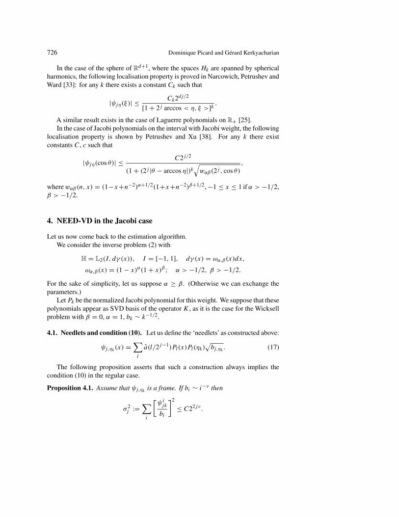
4.1. Needlets and condition (10). Let us define the ‘needlets’ as constructed above:

ψj,ηk (x) =∑l

a(l/2j−1)Pl(x)Pl(ηk)√bj,ηk . (17)

The following proposition asserts that such a construction always implies thecondition (10) in the regular case.

Proposition 4.1. Assume that ψj,ηk is a frame. If bi ∼ i−ν then

σ 2j :=

∑i

[ψijk

bi

]2

≤ C22jν .


Proof. Suppose the family ψj,ηk is a frame (not necessarily tight). As the elements ofa frame are bounded and the set {i, ψijk = 0} is included in the set {C12j , . . . , C22j },we have ∑

i

[ψijk

bi

]2

≤ C2jν‖ψj,ηk‖2 ≤ C′2jν . �

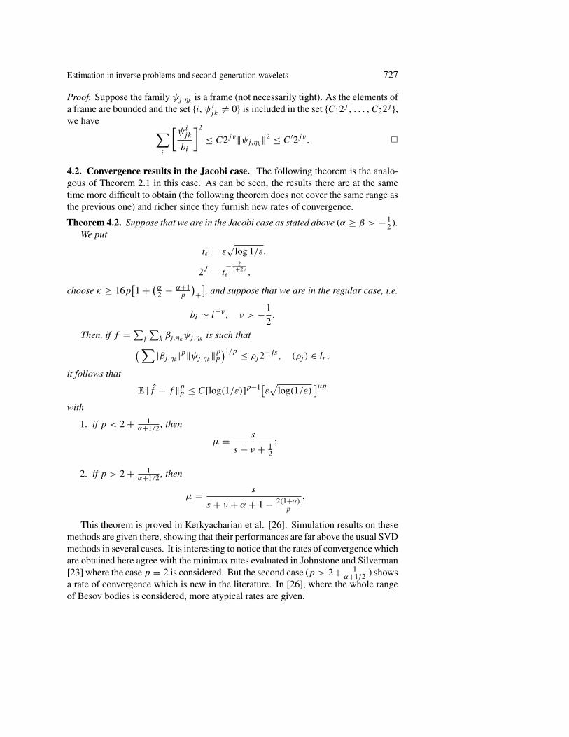
4.2. Convergence results in the Jacobi case. The following theorem is the analo-gous of Theorem 2.1 in this case. As can be seen, the results there are at the sametime more difficult to obtain (the following theorem does not cover the same range asthe previous one) and richer since they furnish new rates of convergence.

Theorem 4.2. Suppose that we are in the Jacobi case as stated above (α ≥ β > − 12 ).

We put

tε = ε√

log 1/ε,

2J = t− 2

1+2νε ,

choose κ ≥ 16p[1 + (

α2 − α+1

p

)+], and suppose that we are in the regular case, i.e.

bi ∼ i−ν, ν > −1

2.

Then, if f = ∑j

∑k βj,ηkψj,ηk is such that( ∑|βj,ηk |p‖ψj,ηk‖pp

)1/p ≤ ρj2−js, (ρj ) ∈ lr ,it follows that

E‖f − f ‖pp ≤ C[log(1/ε)]p−1[ε√log(1/ε)]μp

with

1. if p < 2 + 1α+1/2 , then

μ = s

s + ν + 12

;

2. if p > 2 + 1α+1/2 , then

μ = s

s + ν + α + 1 − 2(1+α)p

.

This theorem is proved in Kerkyacharian et al. [26]. Simulation results on thesemethods are given there, showing that their performances are far above the usual SVDmethods in several cases. It is interesting to notice that the rates of convergence whichare obtained here agree with the minimax rates evaluated in Johnstone and Silverman[23] where the case p = 2 is considered. But the second case (p > 2+ 1

α+1/2 ) showsa rate of convergence which is new in the literature. In [26], where the whole rangeof Besov bodies is considered, more atypical rates are given.


5. Direct models (K = I ): a memento

5.1. The density model. The most famous nonparametric model consists in observ-ing n i.i.d. random variables having a common density f on the interval [0, 1], andin trying to give an estimation of f .

A standard route to perform this estimation consists in expanding the density f inan orthonormal basis {ek, k ∈ N} of a Hilbert space H – assuming implicitly that fbelongs to H:

f =∑l∈N

θlel.

If H happens to be the space L2 = {g : [0, 1] �→ R, ‖g‖22 := ∫ 1

0 g2 < ∞}, we

observe that

θl =∫ 1

0el(x)f (x)dx = Eel(Xi).

Replacing the expectation by the empirical one leads to a standard estimate for θl :

θl = 1

n

n∑i=1

el(Xi).

At this step, the simplest choice of estimate for f is obviously:

fm =m∑i=1

θlel . (18)

5.2. From the density to the white noise model. Before analysing the properties ofthe estimator defined above, let us observe that the previous approach (representingf by its coefficients {θk, k ≥ 0}, leads to summarize the information in the followingsequence model:

{θk, k ≥ 0}. (19)

We can write θk =: θk + uk , with

uk = 1

n

n∑i=1

[ek(Xi)− θk],

The central limit theorem is a relatively convincing argument that the model (19) maybe approximated by the following one:{

θk = θk + ηk√n, k ≥ 0

}, (20)

where the ηk’s are forming a sequence of i.i.d. gaussian, centered variables with fixedvariance σ 2, say. Such an approximation requires more delicate calculations thanthese quick arguments and is rigourously proved in Nussbaum [35], see also Brown


and Low [5]. This model is the sequence space model associated to the followingglobal observation, the so-called white noise model (with ε = n−1/2):

dYt = f (t)dt + εdWt, t ∈ [0, 1],where for anyϕ ∈ L

2([0, 1], dt), ∫[0,1] ϕ(t)dYt = ∫[0,1] f (t)ϕ(t)dt+ε

∫[0,1] ϕ(t)dWt

is observable.(20) formally consists in considering all the observables obtained for ϕ = ek for

all k in N. Among nonparametric situations, the white noise model considered aboveis one of the simplest, at least technically. Mostly for this reason, this model hasbeen given a central place in statistics, particularly by the Russian school, followingIbraguimov and Has’minskii (see for instance their book [20]). However it arisesas an appropriate large sample limit to more general nonparametric models, such asregression with random design, or non independent spectrum estimation, diffusionmodels – see for instance [21], [4],. . . .

5.3. The linear estimation: how to choose the tuning parameter m? In (18), thechoice of m is crucial.

To better understand the situation let us have a look at the risk of the strategy fm.If we consider that, when deciding fm when f is the truth, we have a loss of order‖fm − f ‖2

2, then our risk will be the following mathematical expectation:

E‖fm − f ‖22.

Of course this way of measuring our risk is arguable since there is no particularreason for the L2 norm to reflect well the features we want to recover in the signal.For instance, an L∞-norm could be preferred because it is easier to visualize. Ingeneral, several Lp norms are considered (as it is the case in Sections 2.1 and 4.2).Here we restrict to the L2 case for sake of simplicity.

To avoid technical difficulties, we set ourselves in the case of a white noise model,considering that we observe the sequence defined in (20). Hence,

E(θl − θl)2 = 1

n

∫ 1

0el(x)

2dx = 1

n:= ε2.

We are now able to obtain

E‖fm − f ‖22 =

∑l≤m

(θl − θl)2 +

∑l>m

θ2l ≤ mε2 +

∑l>m

θ2l .

Now assume that f belongs to the following specified compact set of l2:∑l>k

θ2l ≤ Mk−2s for all k ∈ N∗, (21)


for some s > 0 which is here an index of regularity directly connected to the size ofthe compact set in l2 containing the function f . Then we obtain

E‖fm − f ‖22 ≤ mε2 +Mm−2s .

We observe that the RHS is the sum of two factors: one (called the stochastic term)is increasing inm and reflects the fact that because of the noise, the more coefficientswe have to estimate, the larger the global error will be. The second one (called thebias term or approximation term) does not depend on the noise and is decreasing inm.

The RHS is optimised by choosing m = m∗(s) =: c(s,M)ε −21+2s . Then

E‖fm∗(s) − f ‖2 ≤ c′(s,M)ε−4s

1+2s .

Let us observe that the more f is supposed to be regular (in the sense the larger sis), the less coefficients we need to estimate: a very irregular function (s close to 0)requires almost as much as ε−2 = n coefficients, which corresponds to estimate asmany coefficients as the number of available observations – in the density model forinstance. The rate obtained in (5.3) can be proved to be optimal in the following sense(minimax): if we consider the best estimator in its worst performance over the classof functions verifying (21), this estimator attains a rate of convergence which is (upto a constant) the one given in (5.3). See Tsybakov [40] for a detailed review of theminimax point of view.

5.4. The thresholding estimation. Let us now suppose that the constant s, whichplays an essential role in the construction of the previous estimator is not known.This is realistic, since it is extremely rare to know in advance that the function we areseeking has a specified regularity. Also, the previous approach takes very seriouslyinto account the order in which the basis is taken. Let us now present a very elegantway of addressing at the same time both of these issues. The thresholding techniqueswhich have been known for long by engineers in electronic and telecommunications,was introduced in statistics in Donoho and Johnstone [14] and later in a series ofpapers on wavelet thresholding [12], [13]. It allies numerical simplicity to asymptoticoptimality.

It starts from a different kind of observation. Let us introduce the followingestimate:

f =B∑k=0

θkI{|θk| ≥ κtε}ek. (22)

Here the point of view is the following. We choose B very large (i.e. almost corre-sponding to s = 0):

B = ε−2log 1/ε.

But instead of keeping all the coefficients θk such that k is between 0 and B, wedecide to kill those which are not above the threshold tε. The intuitive justification of


this choice is as follows. Assuming that f has some kind of regularity condition like(21) (unknown, but real...), essentially means that the coefficients θk of f are of smallmagnitude except perhaps a small number of them. Obviously, in the reconstructionof f , only the large coefficients will be significant. tε is chosen in such a way that thenoise θk − θk due to the randomness of the observation might be neglected:

tε = ε[log 1/ε]−1/2.

Now let us assume another type of condition on f – easily interpreted by thefact that f is sparsely represented in the basis (ek) – namely: there exists a positiveconstant 0 < q < 2 such that

supλ>0

λq#{k, |θk| ≥ λ} ≤ M for all k ∈ N∗, (23)

E‖f − f ‖22 =

∑l≤B(θlI{|θl| ≥ κtε} − θl)

2 +∑l>B

θ2l

≤∑l

(θl − θl)2I{|θl| ≥ κtε/2} +

∑l

θ2l I{|θl| ≤ 2κtε}

+∑l≤B

[(θl − θl)2 + θ2

l ]I{|θl − θl| ≥ κtε/2} +∑l>B

θ2l .

Now, using the probabilistic bounds

E(θl − θl)2 = ε2, P(|θl − θl| ≥ λ) ≤ 2 exp − λ2

2ε2 for all λ > 0,

and the fact that condition (23) implies∑l

θ2l I{|θl| ≤ 2κtε} ≤ Ct2−q

ε ,

we get

E‖f − f ‖22 ≤ Mε2t−qε + C′t2−q

ε + εκ2/8B +

∑l>B

θ2l .

It remains now to choose κ2 ≥ 32 in order to get

E‖f − f ‖22 ≤ C′t2−q

ε +∑l>B

θ2l ,

and if we assume in addition to (23) that∑l>k

θ2l ≤ Mk− 2−q

2 for all k ∈ N∗, (24)


then we get

E‖f − f ‖22 ≤ C"t2−q

ε

Note that the interesting point in this construction is that the regularity conditionsimposed on the function f are not known by the statistician, since they do not enterinto the construction of the procedure. This property is called adaptation.

Now, to compare with the previous section, let us take q = 21+2s . It is not difficult

to prove that as soon as f verifies (21), it automatically verifies (23) and (24). Hencef and fm∗(s) have the same rate of convergence up to a logarithmic term. If we neglectthis logarithmic loss, we substantially gain here the fact that we need not know theapriori regularity conditions on the aim function. It can also be proved that in factconditions (23) and (24) are defining a set which is substantially larger than the setdefined by condition (21): for instance its entropy is strictly larger (see [28]).

6. Appendix: Proof of Theorem 2.1

In this proof, C will denote an absolute constant which may change from one line tothe other.

We can always suppose p ≥ π . Indeed, if π ≥ p it is very simple to see

that Bsπ,r (M) is included into Bsp,r (M): as 2j [s+12 − 1

p]‖βj ·‖lp ≤ 2j [s+ 1

2 − 1π

]‖βj ·‖lπ(since χj is of cardinality 2j ).

First we have the following decomposition:

E‖f − f ‖pp ≤ 2p−1{E

∥∥∥ J∑j=−1

∑k∈χj

(t (βjk)− βjk)ψjk

∥∥∥pp

+∥∥∥ ∑j>J

∑k∈χj

βjkψjk

∥∥∥pp

}=: I + II.

The term II is easy to analyse: since f belongs toBsπ,r (M), using standard embeddingresults (which in this case simply follows from direct comparisons between lq norms)

we have that f also belong to Bs−( 1

π− 1p)+

p,r (M ′), for some constant M ′. Hence∥∥∥ ∑j>J

∑k∈χj

βjkψjk

∥∥∥p

≤ C2−J [¯s−( 1

π− 1p)+].

Then we only need to verify thats−( 1

π− 1p)+

1+2ν is always larger that α, which is notdifficult.

Bounding the term I is more involved. Using the triangular inequality together


with Hölder’s inequality and property (8) for the second line, we get

I ≤ 2p−1Jp−1J∑

j=−1

E

∥∥∥ ∑k∈χj

(t (βjk)− βjk)ψjk

∥∥∥pp

≤ 2p−1Jp−1Dp

J∑j=−1

∑k∈χj

E|t (βjk)− βjk|p‖ψjk‖pp .

Now, we separate four cases:

J∑j=−1

∑k∈χj

E|t (βjk)− βjk|p‖ψjk‖pp

=J∑

j=−1

∑k∈χj

E|t (βjk)− βjk|p‖ψjk‖pp{I {|βjk| ≥ κtεσj } + I {|βjk| < κtεσj }

}

≤J∑

j=−1

∑k∈χj

[E|βjk − βjk|p‖ψjk‖ppI {|βjk| ≥ κtεσj }{I{|βjk| ≥ κ

2tεσj

}+ I

{|βjk| < κ

2tεσj

}}+ |βjk|p‖ψjk‖ppI {|βjk| ≤ κtεσj }{I {|βjk| ≥ 2κtεσj } + I {|βjk| < 2κtεσj }

}]≤: Bb + Bs + Sb + Ss.

Notice that βjk − βjk = ∑iYi−bifibi

ψijk = ε∑i ξi

ψijkbi

is a centered gaussian random

variable with variance ε2 ∑i

[ψijkbi

]2. Also recall that we set σ 2j =: ∑

i[ψijkbi

]2 ≤ C22jν

and denote by sq the qth absolute moment of the gaussian distribution when centeredand with variance 1. Then, using standard properties of the gaussian distribution, forany q ≥ 1 we have

E|βjk − βjk|q ≤ sqσqj ε

q, P{|βjk − βjk| ≥ κ

2tεσj } ≤ 2εκ

2/8.

Hence

Bb ≤J∑

j=−1

∑k∈χj

spσpj ε

p‖ψjk‖ppI {|βjk| ≥ κ

2tεσj },

Ss ≤J∑

j=−1

∑k∈χj

|βjk|p‖ψjk‖ppI {|βjk| < 2κtεσj }


and

Bs ≤J∑

j=−1

∑k∈χj

[E|βjk − βjk|2p]1/2[P

{|βjk − βjk| ≥ κ

2tεσj

}]1/2

‖ψjk‖ppI{|βjk| < κ

2tεσj

}≤

J∑j=−1

∑k∈χj

s1/22p σ

pj ε

p21/2εκ2/16‖ψjk‖ppI

{|βjk| < κ

2tεσj

}

≤ C

J∑j=−1

2jp(ν+12 )εpεκ

2/16 ≤ Cεκ2/16.

Now, if we remark that the βjk’s are necessarily all bounded by some constant (de-pending on M) since f belongs to Bsπ,r (M), and using (7),

Sb ≤J∑

j=−1

∑k∈χj

|βjk|p‖ψjk‖ppP{|βjk − βjk| ≥ 2κtεσj }I {|βjk| ≥ 2κtεσj }

≤J∑

j=−1

∑k∈χj

|βjk|p‖ψjk‖pp2εκ2/8I {|βjk| ≥ 2κtεσj }

≤ C

J∑j=−1

2jp2 εκ

2/8 ≤ Cεκ28 − p

2(2ν+1) .

It is easy to check that in all cases, if κ2 ≥ 16p the terms Bs and Sb are smallerthan the rates given in the theorem.

Using (7) and condition (10), for any z ≥ 0 we have

Bb ≤ CεpJ∑

j=−1

2j (νp+ p2 −1)

∑k∈χj

I{|βjk| ≥ κ

2tεσj

}

≤ CεpJ∑

j=−1

2j (νp+ p2 −1)

∑k∈χj

|βjk|z[tεσj ]−z

≤ Ctεp−z

J∑j=−1

2j [ν(p−z)+ p2 −1] ∑

k∈χj|βjk|z.


Also, for any p ≥ z ≥ 0,

Ss ≤ C

J∑j=−1

2j (p2 −1)

∑k∈χj

|βjk|zσp−zj [tε]p−z

≤ C[tε]p−zJ∑

j=−1

2j (ν(p−z)+ p2 −1)

∑k∈χj

|βjk|z.

So in both cases we have the same bound to investigate. We will write this boundin the following form (forgetting the constant):

I + II = tεp−z1

[ j0∑j=−1

2j [ν(p−z1)+ p2 −1] ∑

k∈χj|βjk|z1

]

+ tεp−z2

[ J∑j=j0+1

2j [ν(p−z2)+ p2 −1] ∑

k∈χj|βjk|z2

].

The constants zi and j0 will be chosen depending on the cases.Let us first consider the case where s ≥ (

ν + 12

)(pπ

− 1). Put

q = p(2ν + 1)

2(s + ν)+ 1

and observe that, on the considered domain, q ≤ π and p > q. In the sequel it willbe used that we automatically have s = (

ν + 12

)(pq

− 1). Taking z2 = π we get

II ≤ tεp−π[ J∑

j=j0+1

2j [ν(p−π)+ p2 −1] ∑

k∈χj|βjk|π

].

Now, asp

2q− 1

π+ ν

(p

q− 1

)= s + 1

2− 1

π

and ∑k∈χj

|βjk|π = 2−j (s+ 12 − 1

π)τj

with (τj )j ∈ lr (this is a consequence of the fact that f ∈ Bsπ,r (M) and (6)), we canwrite

II ≤ tεp−π ∑

j=j0+1

2jp(1− πq)(ν+ 1

2 )τπj

≤ Ctεp−π2j0p(1− π

q)(ν+ 1

2 ).


The last inequality is true for any r ≥ 1 if π > q and for r ≤ π if π = q. Noticethat π = q is equivalent to s = (ν + 1

2 )(pπ

− 1). Now if we choose j0 such that

2j0pq(ν+ 1

2 ) ∼ tε−1 we get the bound

tεp−q

which exactly gives the rate asserted in the theorem for this case.As for the first part of the sum (before j0), we have, taking now z1 = q, with

q ≤ π , so that[ 1

2j∑k∈χj |βjk|q

] 1q ≤ [ 1

2j∑k∈χj |βjk|π

] 1π , and using again (6),

I ≤ tεp−q[ j0∑

−1

2j [ν(p−q)+ p2 −1] ∑

k∈χj|βjk|q

]

≤ tεp−q[ j0∑

−1

2j [ν(p−q)+ p2 − q

π] ∑k∈χj

|βjk|π ] qπ]

≤ tεp−q

j0∑−1

2j [(ν+12 )p(1− q

q)]τqj

≤ Ctεp−q2j0[(ν+ 1

2 )p(1− qq)]

≤ Ctεp−q .

The last two lines are valid if q is chosen strictly smaller than q (this is possible sinceπ ≥ q).

Let us now consider the case where s <(ν + 1

2

)(pq

− 1), and choose

q = p

2(s + ν − 1

π

) + 1

in such a way that we easily verify thatp−q = 2 s−1/π+1/p1+2(ν+s−1/π) , q−π = (p−π)(1+2ν)

2(s+ν− 1

π

)+1>

0, because s is supposed to be larger than 1π

. Furthermore we also have s + 12 − 1

π=

p2q − 1

q+ ν

(pq

− 1).

Hence taking z1 = π and using again the fact that f belongs to Bsπ,r (M),

I ≤ tεp−π[ j0∑

−1

2j [ν(p−π)+ p2 −1] ∑

k∈χj|βjk|π

]

≤ tεp−π

j0∑−1

2j [(ν+12 − 1

p)pq(q−π)]

τπj

≤ Ctεp−π2j0[(ν+ 1

2 − 1p)pq(q−π)]

.


This is true since ν + 12 − 1

pis also strictly positive because of our constraints. If we

now take 2j0pq(ν+ 1

2 − 1p) ∼ tε

−1 we get the bound

tεp−q

which is the rate stated in the theorem for this case.Again, for II, we have, taking now z2 = q > q (> π),

II ≤ tεp−q[ J∑

j=j0+1

2j [ν(p−q)+ p2 −1] ∑

k∈χj|βjk|q

]≤ Ctε

p−q ∑j=j0+1

2j [(ν+12 − 1

p)pq(q−q)]

zqπ

j

≤ Ctεp−q2j0[(ν+ 1

2 − 1p)pq(q−q)]

≤ Ctεp−q .

References

[1] Abramovich, F., and Silverman, B. W., Wavelet decomposition approaches to statisticalinverse problems. Biometrika 85 (1) (1998), 115–129 .

[2] Antoniadis, A., and Bigot, J., Poisson inverse models. Preprint, Grenoble 2004.

[3] Antoniadis, A., Fan,J., and Gijbels, I., A wavelet method for unfolding sphere size distri-butions. Canad. J. Statist. 29 (2001), 251–268.

[4] Brown, Lawrence D., Cai, T. Tony, Low, Mark G., and Zhang, Cun-Hui Asymptotic equiv-alence theory for nonparametric regression with random design. Ann. Statist. 30 (3) (2002),688–707.

[5] Brown, Lawrence D., and Low, Mark G., Asymptotic equivalence of nonparametric re-gression and white noise. Ann. Statist. 24 (6) (1996), 2384–2398.

[6] Cavalier, Laurent, and Tsybakov, Alexandre, Sharp adaptation for inverse problems withrandom noise. Probab. Theory Related Fields 123 (3) (2002), 323–354.

[7] Cavalier, L., Golubev, G. K., Picard, D., and Tsybakov., A. B., Oracle inequalities forinverse problems. Ann. Statist. 30 (3) (2002), 843–874.

[8] Cohen, Albert, Hoffmann, Marc, and Reiß, Markus, Adaptive wavelet Galerkin methodsfor linear inverse problems. SIAM J. Numer. Anal. 42 (4) (2004), 1479–1501 (electronic).

[9] Cruz-Orive, L. M., Distribution-free estimation of sphere size distributions from slabsshowing overprojections and truncations, with a review of previous methods. J. Microscopy131 (1983), 265–290.

[10] Dicken, V., and Maass, P., Wavelet-Galerkin methods for ill-posed problems. J. InverseIll-Posed Probl. 4 (3) (1996), 203–221.

[11] Donoho, David L., Nonlinear solution of linear inverse problems by wavelet-vaguelettedecomposition. Appl. Comput. Harmon. Anal. 2 (2) (1995), 101–126.


[12] Donoho, D. L., Johnstone, I. M., Kerkyacharian, G., and Picard, D., Wavelet shrinkage:Asymptopia? J. Royal Statist. Soc. Ser. B 57 (1995), 301–369.

[13] Donoho, D. L., Johnstone, I. M., Kerkyacharian, G., and Picard, D., Density estimation bywavelet thresholding. Ann. Statist. 24 (1996), 508–539.

[14] Donoho, D. L., Johnstone, I. M., Minimax risk over �p-balls for �q -error. Probab. TheoryRelated Fields 99 (1994), 277–303.

[15] Duffin, R. J., and Schaeffer, A. C., A class of nonharmonic Fourier series. Trans. Amer.Math. Soc. 72 (1952), 341–366.

[16] Efromovich, Sam, and Koltchinskii, Vladimir, On inverse problems with unknown opera-tors. IEEE Trans. Inform. Theory 47 (7) (2001), 2876–2894.

[17] Fan, J., and Koo, J. K., Wavelet deconvolution. IEEE Trans. Inform. Theory 48 (3) (2002),734–747.

[18] Frazier, M., Jawerth, B., and Weiss, G., Littlewood-Paley theory and the study of functionspaces. CBMS Reg. Conf. Ser. Math. 79, Amer. Math. Soc., Providence, RI, 1991.

[19] Goldenshluger, Alexander, and Pereverzev, Sergei V., On adaptive inverse estimation oflinear functionals in Hilbert scales. Bernoulli 9 (5) (2003), 783–807.

[20] Ibragimov, I. A., and Hasminskii, R. Z., Statistical estimation. Appl. Math. 16, Springer-Verlag, New York 1981.

[21] Jähnisch, Michael, and Nussbaum, Michael, Asymptotic equivalence for a model of inde-pendent non identically distributed observations. Statist. Decisions 21 (3) (2003), 197–218.

[22] Johnstone, Iain M., Kerkyacharian, Gérard, Picard, Dominique, and Raimondo, Marc,Wavelet deconvolution in a periodic setting. J. R. Stat. Soc. Ser. B Stat. Methodol. 66 (3)(2004), 547–573.

[23] Johnstone, Iain M., and Silverman, Bernard W., Discretization effects in statistical inverseproblems. J. Complexity 7 (1) (1991), 1–34.

[24] Kalifa, Jérôme, and Mallat, Stéphane, Thresholding estimators for linear inverse problemsand deconvolutions. Ann. Statist. 31 (1) (2003), 58–109.

[25] Kerkyacharian, G., Petrushev, P., Picard, D., and Xu,Y., Localized polynomials and framesinduced by laguerre functions. Preprint, 2005.

[26] Kerkyacharian, G., Picard, D., Petrushev, P., and Willer, T., Needvd: second generationwavelets for estimation in inverse problems. Preprint, LPMA 2006.

[27] Kerkyacharian, G., Picard, D., and Raimondo, M., Adaptive boxcar deconvolution on fulllebesgue measure sets. Preprint, LPMA 2005.

[28] Kerkyacharian, G., and Picard, D., Thresholding algorithms and well-concentrated bases.Test 9 (2) (2000).

[29] Mair, Bernard A., and Ruymgaart, Frits H., Statistical inverse estimation in Hilbert scales.SIAM J. Appl. Math. 56 (5) (1996), 1424–1444.

[30] Mallat, Stéphane, A wavelet tour of signal processing. Academic Press Inc., San Diego,CA, 1998.

[31] Mathé, Peter, and Pereverzev, Sergei V., Geometry of linear ill-posed problems in variableHilbert scales. Inverse Problems 19 (3) (2003), 789–803.

[32] Meyer,Yves, Ondelettes et opérateurs. I. Actualités Mathématiques. Hermann, Paris 1990.


[33] Narcowich, F. J., Petrushev, P., and Ward, J. M., Localized tight frames on spheres. SIAMJ. Math. Anal. 38 (2) (2006), 574–594.

[34] Neelamani, R., Choi, H., and Baranuik, R., Wavelet-based deconvolution for ill-condi-tioned systems. Preprint, 2000; http://www-dsp.rice.edu/publications/pub/neelsh98icassp.pdf.

[35] Nussbaum, Michael, Asymptotic equivalence of density estimation and Gaussian whitenoise. Ann. Statist. 24 (6) (1996), 2399–2430.

[36] Nyshka, D., Wahba, G., Goldfarb, S., and Pugh, T., Cross validated spline methods forthe estimation of three-dimensional tumor size distributions from observations on two-dimensional cross sections. J. Amer. Statist. Assoc. 79 (1984), 832–8464.

[37] Pensky, M., and Vidakovic, B., Adaptive wavelet estimator for nonparametric densitydeconvolution. Ann. Statist. 27 (1999), 2033–2053.

[38] Petrushev, P., and Xu,Y., Localized polynomials frames on the interval with jacobi weights.J. Fourier Anal. Appl. 11 (5) (2005), 557–575.

[39] Petrushev, P., and Xu, Y., Localized polynomials kernels and frames (needlets) on the ball.2005. IMI 2005.

[40] Tsybakov, Alexandre B., Introduction à l’estimation non-paramétrique. Math. Appl.(Berlin) 41, Springer-Verlag, Berlin 2004.

[41] Tsybakov, Alexandre, On the best rate of adaptive estimation in some inverse problems. C.R. Acad. Sci. Paris Sér. I Math. 330 (9) (2000), 835–840.

[42] Wicksell, S. D., The corpuscle problem: a mathematical study of a biometric problem.Biometrika 17 (1925), 84–99.

[43] Willer, T., Deconvolution in white noise with a random blurring effect. Preprint, LPMA2005.

LPMA, Universités Paris VII et Paris X, CNRS, 175 rue du Chevaleret, 75013 Paris, France

Estimation in inverse problems and second-generation wavelets

Documents

Transcript of Estimation in inverse problems and second-generation wavelets