Estimation for State-Space Models; anApproximate Likelihood Approach

Richard A. Davis and Gabriel Rodriguez-YamDepartment of Statistics, Colorado State University, Fort Collins, Colorado

October 22, 2003

Abstract

Typically, the likelihood function for non-Gaussian state-space modelscan not be computed explicitly and so simulation based procedures, suchas importance sampling or MCMC, are commonly used to estimate modelparameters. In this paper, we consider an alternative estimation procedurewhich is based on an approximation to the likelihood function. The approx-imation can be computed and maximized directly, resulting in a quick esti-mation procedure without resorting to simulation. Moreover, this approachis competitive with estimates produced using simulation-based procedures.The speed of this procedure makes it viable to fit a wide range of potentialmodels to the data and allows for bootstrapping the parameter estimates.

1 Introduction

The class of state-space models (SSM) provides a flexible framework for modelingand describing a wide range of time series in a variety of disciplines. The booksby Harvey (1989) and Durbin and Koopman (2001) contain extensive accounts ofstate-space models and their applications. One of the attractive features of state-space models is that many traditional models, such as ARMA and ARIMA, can beexpressed in a linear state-space system. For linear and/or Gaussian state-spacemodels, the Kalman filter can be used to compute predictors of the state-variablesand one-step-ahead predictors of the observations. This allows for straightforwardcalculation of the likelihood in the Gaussian case. However, in many applicationsin which the Gaussian assumption is not realistic, the likelihood function is difficultto calculate, which makes maximum likelihood estimation problematic.

The state-space model that we consider in this paper has the following formu-lation: If Y1, Y2, . . . , represent the time series of observations and α1, α2, . . . therespective “state variables”, then it is assumed that

p(yt|αt, αt−1, . . . , α1, yt−1, . . . , y1) = p(yt|αt) (1)

1

belongs to a known parametric family of distributions. In addition, the state processis assumed to follow an AR(p) model, given by

αt = γ + φ1αt−1 + . . . + φpαt−p + ηt, (2)

where p is an integer greater than zero and ηt ∼ iid N(0, σ2), t = 1, 2, . . .. Perhapsthe most important special case is when the conditional distribution in (1) is amember of the exponential family, an extremely rich class of distributions. Durbinand Koopman (1997) and Kuk (1999), consider the following form for this family

p(yt|αt) = e(xTt β+αt)yt−b(xT

t β+αt)+c(yt), (3)

where xt is a vector of covariates observed at time t; β is a vector of parameters;and b(.) and c(.) are known real functions.

One special application that we will consider in more detail, is the case in whichthe time series Y1, . . . , Yn consist of counts. Here, it might be plausible to modelYt by a Poisson distribution with rate λt := eαt+xT

t β in which case, p(yt|αt; β) is aparticular case of (3). Models of this type have been used for modeling counts ofindividuals infected by a rare disease, e.g., Zeger (1988); Campbell (1994); Chanand Ledolter (1995); Harvey and Fernandes (1989); Davis et al. (1998).

Another noteworthy application of the SSM that we will consider, is the stochas-tic volatility model (SVM), a frequently used model for returns of financial assets.In the basic SVM, the distribution of Yt|αt is Gaussian with mean 0 and varianceeαt . Applications, together with estimation for SVMs, can be found in Jacquier, etal. (1994); Briedt and Carriquiry (1996); Harvey and Streibel (1998); Sandmannand Koopman (1998); Geweke and Tanizaki (1999); Pitt and Shepard (1999).

Let y := (y1, . . . , yn) denote the vector of observations, α := (α1, . . . , αn) thevector of states and ψ := (θ, λ) the parameters in the state-space model. Here θ isthe vector of the parameters associated with the specification of p(yt|αt), which mayinclude the regression parameter β, and λ := (φ1, . . . , φp, γ, σ2) is the parametervector associated with the AR model in (2). With this specification, the likelihoodbased on the “complete data” (y, α) of the SSM becomes

L(ψ;y,α) = p(y|α, θ)p(α|λ) (4)

=

(n∏

t=1

p(yt|αt, θ)

)|V|1/2e−(α−µ)T V(α−µ)/2/(2π)n/2,

where V−1 := cov{α}, µ = γ/(1 − φ1 − . . . − φp)1 is the vector of means of thestate process, and 1 is a vector of ones. From (4) it follows that the likelihood ofthe observed data is

L(ψ;y) =

∫L(ψ;y,α)dα. (5)

Except in simple cases, the integral in (5) can not be computed explicitly,which makes maximum likelihood estimation difficult. There are several simulation

2

approaches in the literature for estimating and ultimately maximizing this likeli-hood. For example, Durbin and Koopman (1997, 2001) use importance samplingto estimate (5). The observation density p(y|α; θ) is approximated by selectinga Gaussian density g(y|α; θ) that best approximates p(y|α; θ). The Monte Carlointegration is computed using g(α|y; ψ), the conditional density of α relative tothe working model, as the importance density. This approach is known as “manysamples” because for distinct values of ψ, the importance function g(α|y; ψ) is up-dated during the optimization of the approximate observed likelihood. To overcomethe instability problem inherent with the “many samples” approach, Durbin andKoopman generate from the same noise. Kuk (1999) advocates a “single-sample”approach, which for a fixed ψ0, a sample is drawn from the importance densityg(α|y,ψ0) and then the relative likelihood function is optimized using these sam-ples. To get better approximations of the relative likelihood near the true maximumlikelihood estimate, Geyer (1996) suggests repeating the process several times, up-dating ψ0 with the new maximizer at each iteration.

A Monte Carlo EM algorithm treating the unobserved α’s as missing values wasproposed by Chan and Ledolter (1995). At the i -th iteration of the algorithm, theM -step is performed by Monte Carlo integration drawing a sample from the con-ditional distribution p(α|y,ψ(i−1)), where ψ(i−1) is the maximizer obtained in theprevious iteration. Kuk and Cheng (1997) proposed a Monte Carlo implementationof the Newton-Raphson (MCNR) as a viable alternative to the MCEM algorithm.All of these simulation based procedures can be computationally intense.

In this paper we will follow a different approach to obtain an approximation tothe distribution p(α|y; ψ). In Section 2 we will produce an analytical approxima-tion to (5) by obtaining an approximation pa(α|y; ψ) to the posterior distributionp(α|y; ψ). The innovations algorithm (Brockwell and Davis, 1991) can be usedto speed up the computation of these approximations. The approximation to theobserved likelihood can then be maximized to produce an estimate of ψ. In Section3 we demonstrate the good performance of this procedure via simulation studies.This procedure will also be applied to analyze two datasets; the monthly numberof U.S. cases of poliomyelitis for 1970 to 1983 (Zeger, 1988) is analyzed using aPoisson state-space model and a historical pound to dollar exchange rates (Harvey,et al., 1994) is analyzed using a stochastic volatility model.

The quality of our approximation depends, to a large extent, on the normalapproximation to the posterior, p(α|y; ψ). In a numerical example we assess thisapproximation in two ways. First, we notice the closeness between the posteriormode and posterior mean of p(α|y; ψ). As a second check of closeness we comparesamples generated from p(α|y; ψ) using sampling importance resampling (SIR)with the approximating normal distribution via a Chi-squared QQ-plot and a cor-relation test. These topics, together with bootstrap bias correction are consideredin Section 3. In Section 4 we summarize our findings. Application of the inno-vations algorithm to the problems considered in Sections 2 and 3 is given in theappendix.

3

2 Parameter Estimation

In this section we find an approximation to the observed likelihood L(ψ;y) givenin (5) that is based on an approximation La(ψ;y,α) to the likelihood L(ψ;y,α)using the complete data. For the latter, a Taylor series expansion of log p(y|α; θ)in a neighborhood of the posterior mode of p(α|y; ψ) is used.

To begin, let `(θ;y|α) := log p(y|α; θ). Note that the log of the observedlikelihood is given by

`(ψ;y,α) = −n

2log(2π) +

1

2log |V|+ `(ψ;y|α)− 1

2(α− µ)TV(α− µ). (6)

Now, let

k∗ :=∂

∂α`(θ;y|α)|α=α∗

where α∗ is the mode of `(ψ;y,α), which solves ∂∂α

`(ψ;y,α) = 0. From (4), itfollows that

k∗ = V(α∗ − µ),

hence, if T (α; α∗) denotes the second order Taylor expansion of `(θ;y|α) aroundα∗ and R(α; α∗) := `(θ;y|α)− T (α; α∗) the corresponding remainder, then

`(ψ;y|α) = T (α; α∗) + R(α; α∗),

= h∗ + (α−α∗)Tk∗ − 1

2(α−α∗)TK∗(α−α∗) + R(α; α∗),

= h∗ + (α∗ − µ)TV(α−α∗)− 1

2(α−α∗)TK∗(α−α∗) (7)

+ R(α; α∗),

where

h∗ := `(θ;y|α)|α=α∗ and K∗ := − ∂2

∂α∂αT`(θ;y|α)|α=α∗ . (8)

Thus, substituting (7) in (6), it follows that

`(ψ;y,α) = −n

2log(2π) +

1

2log |V|+ h∗ − 1

2(α∗ − µ)TV(α∗ − µ) (9)

−1

2(α−α∗)T (K∗ + V)(α−α∗) + R(α; α∗).

We note that the posterior p(α|y; ψ) satisfies p(α|y; ψ) ∝ L(ψ;y,α). Let pa(α|y; ψ)be the posterior based on the log likelihood given in (9) when the term R(α; α∗)is omitted, it follows that

pa(α|y; ψ) = φ(α; α∗, (K∗ + V)−1), (10)

where φ(.; µ,Σ) is the multivariate normal density with mean µ and covariancematrix Σ. Hence

L(ψ;y) =|V|1/2

|K∗ + V|1/2eh∗− 1

2(α∗−µ)T V(α∗−µ)

∫eR(α;α∗)pa(α|y; ψ)dα, (11)

= La(ψ;y)Era(ψ),

4

where La(ψ;y) is the approximation to L(ψ;y)

La(ψ;y) :=|V|1/2

|K∗ + V|1/2eh∗− 1

2(α∗−µ)T V(α∗−µ), (12)

that is obtained when the factor eR(α;α∗) is ignored in the integral in (11); andEra(ψ) is the approximation error

Era(ψ) :=

∫eR(α;α∗)pa(α|y; ψ)dα. (13)

Thus, if pa(α|y; ψ) is highly concentrated around α∗, the integral in (13) shouldbe close to 1.

Since the evaluation of (12) does not involve simulation, it can be maximizedto obtain an approximate MLE of ψ. In fact, we will see later that both thecomputation of α∗ and the evaluation of (12) can be accelerated with the aid ofthe innovations algorithm (Brockwell and Davis, 1991).

A second way to motivate our approximation La(ψ;y) is based on a Bayesianviewpoint. If we treat α as the parameters of the system with prior p(α|λ), then un-der regularity conditions and a fixed number of parameters, the posterior p(α|y; ψ)can be approximated by a normal density function for n large (e.g., Bernardo andSmith, 1994; page 287). This normal density matches the mode of the posteriorp(α|y; ψ) and has covariance matrix equal to the inverse of the information matrixof the posterior evaluated at the posterior’s mode. Notice that α∗ is the mode ofthe posterior p(α|y; ψ) and the observed information matrix is given by K∗ + V.Both assertions can be obtained from the fact that p(α|y; ψ) ∝ L(ψ;y, α). Thus,is this context, the normal approximation is, in fact, the same as pa(α|y; ψ) givenin (10).

We note that

L(ψ;y) =

∫p(y|α; θ)p(α|λ)dα,

=

∫p(y|α; θ)p(α|λ)

pa(α|y; ψ)pa(α|y; ψ)dα. (14)

So, pa(α|y; ψ) in (10) can be viewed as an importance density.Now, we provide a recursive algorithm to find α∗, the mode of p(α|y; ψ). Let

αj be the current iterate to the value of α∗. If

kj :=∂

∂α`(θ;y|α)|α=αj and Kj := − ∂2

∂α∂αT`(θ;y|α)|α=αj , (15)

then the Newton-Raphson algorithm gives

αj+1 = αj − (¨j)−1 ˙j, (16)

5

where

˙j :=∂

∂α`(ψ;y,α)|α=αj

= kj −V(αj − µ)

= kj + Kjαj + Vµ− (Kj + V)αj, (17)

¨j := (∂2

∂α∂αT`(ψ;y,α))−1|α=αj

= −Kj −V. (18)

Letyj := kj + Kjαj + Vµ. (19)

Substituting this, (17) and (18) into (16), we obtain

αj+1 = (Kj + V)−1yj. (20)

Application to the exponential family

Assume that the observation density function is from the exponential family givenby

p(y|α; θ) =n∏

t=1

p(yt|αt,θ) = e(xβ+α)T y−1T {b(xβ+α)−c(y)}, (21)

where b(xβ+α) := [b(xT1 β+α1), . . . , b(x

Tnβ+αn)]T and c(y) := [c(y1), . . . , c(yn)]T .

In this setting, the matrix K∗ in (8) becomes

K∗ = diag{ ∂2

∂α2t

b(xTt β + αt)|α∗t }. (22)

The approximation to the observed likelihood is then

La(ψ;y) =|V|1/2

|K∗ + V|1/2eyT (xβ+α∗)−1T {b(xβ+α∗)−c(y)}−(α∗−µ)T V(α∗−µ)/2. (23)

From (15) and (21), kj = y − bj, where

bj :=∂

∂α1Tb(xβ + α)|αj . (24)

Hence,yj := y − bj + Kjαj + Vµ, (25)

where Kj is defined in (15). ¤

Although at this point we can find an approximation to the likelihood, eachiteration of (20) needs the inversion of a matrix of dimension n × n, while each

6

evaluation of (12) requires calculation of the determinant of a matrix of similardimension. For small values of n, these computations can be carried out directly,but for large values, direct computations are impractical. Recursive predictionalgorithms, such as the Kalman recursions or the innovations algorithm acceleratethese calculations. Here we use the innovations algorithm, which seems to be ideallysuited for this problem. The implementation of the innovation algorithm in thiscontext is described in the Appendix.

As we noted from (14), pa(α|y; ψ) in (10) can be used as an importance density.In fact, as we show below for the case of the exponential family of distributions,pa(α|y; ψ) coincides with the importance density function of Durbin and Koop-man (1997) to estimate the likelihood in (5) via simulation. In order to describetheir method, let Lg(ψ) denote the likelihood of the Gaussian approximating modelof the state-space model proposed by Durbin and Koopman (1997). Such an ap-proximation is obtained when p(yt|αt; ψ) is replaced by a Gaussian distributiong(yt|αt; θ) = φ(yt; Ztαt + µt, Ht), where µt and Ht are found by solving iteratively

∂

∂αt

log p(yt|αt; ψ)|αt=αt −H−1t (yt − αt − µt) = 0 (26)

∂2

∂α2t

log p(yt|αt; ψ)|αt=αt + H−1t = 0. (27)

Here, the αt are found by routine application of the Kalman filtering and smoothingalgorithms. The iterations, initialized with µt = 0 and Ht arbitrary, must bestopped until convergence of µt and Ht. Let Eg denote the conditional expectationoperator under the approximating model. Durbin and Koopman (1997) found thatthe likelihood (5) can be expressed as

L(ψ) = Lg(ψ)Eg

{p(y|α,θ)

g(y|α, ψ)|y,ψ

}. (28)

Hence, with simulated values α(1), . . . , α(N) from the conditional density g(α|y; ψ)under the approximating model, the integral in (5) is estimated as

L(ψ) = Lg(ψ)1

N

N∑i=1

p(y|α(i),θ)

g(y|α(i), ψ). (29)

This method is called a “many samples” approach, because new simulatedvalues of the α(i)’s are needed for each value of ψ. To ensure stability in theirnumerical process, they generate from the noise only once.

Alternatively, Kuk (1999) proposes using the relative likelihood

L(ψ)

Lg(ψ0)= Eg

{p(y, α|ψ)

g(y,α|ψ0)|y,ψ0

}, (30)

where the conditional expectation is computed relative to the conditional densityg(α|y,ψ0) under the approximating model. Using simulated values α(1), . . . , α(N)

7

from the conditional density g(α|y,ψ0), an estimate of L(ψ) using (30) is

L(ψ) = Lg(ψ0)1

N

N∑i=1

p(y|α(i),θ)p(α(i)|λ)

g(y|α(i),θ0)p(α(i)|λ0). (31)

This approach is known as a “single-sample” procedure, since it involves sim-ulating from g(α|y,ψ0) instead of g(α|y; ψ). In order for this method to work, afew updatings of ψ0 to the optimizer of L(ψ) in (31) is recommended (Geyer, 1996;Kuk, 1999).

If p(yt|αt; ψ) is a member of the exponential family of distributions as givenin (3), then using the notation bt := ∂

∂αtb(xT

t β + αt)|αt=αt and bt := ∂2

∂α2tb(xT

t β +

αt)|αt=αt , Durbin and Koopman (1997) find that

H−1t = bt, µt = yt − αt − b−1

t (yt − bt). (32)

They comment that α := [α1, . . . , αn]T , obtained using the iterative proceduredescribed above, is the posterior mode of p(α|y; ψ). We conclude that α = α∗.Furthermore, from (32), it follows that the variance of the distribution g(α|y; ψ)computed under the approximating model until convergence is achieved is given by(K∗+V)−1, where K∗ is given in (22). Thus, pa(α|y; ψ) in (10) and g(α|y,ψ) areidentical. As a result, the observed likelihood Lg(ψ) of the Durbin and Koopman’sapproximate Gaussian model is given by

Lg(ψ) = (2π)−n/2|b∗|1/2e1T {b(xβ+α∗)−c(y)}−yT α∗−{y−b∗}T (b∗)−1{y−b∗}/2La(ψ;y),(33)

where b∗ := ∂∂α

1Tb(xβ + α)|α∗ , and b∗ := ∂2

∂α∂αT 1Tb(xβ + α)|α∗ .

To get a feel for how these two procedures perform, we consider the case whenthe observation density is Poisson with rate λt = e0.7+αt and the state processfollows the AR(1) model

αt = φαt−1 + ηt, (34)

where ηt ∼ iid N(0, 0.3), t = 1, . . . , n = 200. In this example, the state-space modelhas only one parameter, i.e., ψ = φ. Using φ = 0.5, one realization y1, . . . , y200 fromthis process was generated. In Figure 1 we show two estimates of the observedlikelihood of this process. In this figure, the solid line is the approximation to theobserved likelihood given in (23). Also, the lower and upper dotted lines, computedfor each value of φ in a grid of points, are the minimum and maximum, respectively,of 100 replicates of the estimated likelihood given in (29) using N = 1000. Thedashed line is an estimation of the likelihood using (29) for one of these realizations.The pair of dotted lines in this figure illustrate the randomness of the estimationof φ that is obtained by the maximization of (29). The shape of the dashed line inFigure 1, typical of the estimator in (29), comes from the “many samples” effect.The maximization of this random function to obtain an estimator of φ requires

8

phi

log

like

liho

od

0.3 0.4 0.5 0.6 0.7

-34

2-3

41

-34

0-3

39

Figure 1: (Many samples) For a grid of values of φ, the logarithm of the estimation ofthe likelihood of a Poisson SSM are shown. For the solid line, estimates were obtainedusing (23) while for the dashed line, (29) was used. The dotted lines are the minimumand maximum respectively, of 100 replicates using (29).

additional effort. In contrast, the approximation in (23) is smooth and can becomputed much faster.

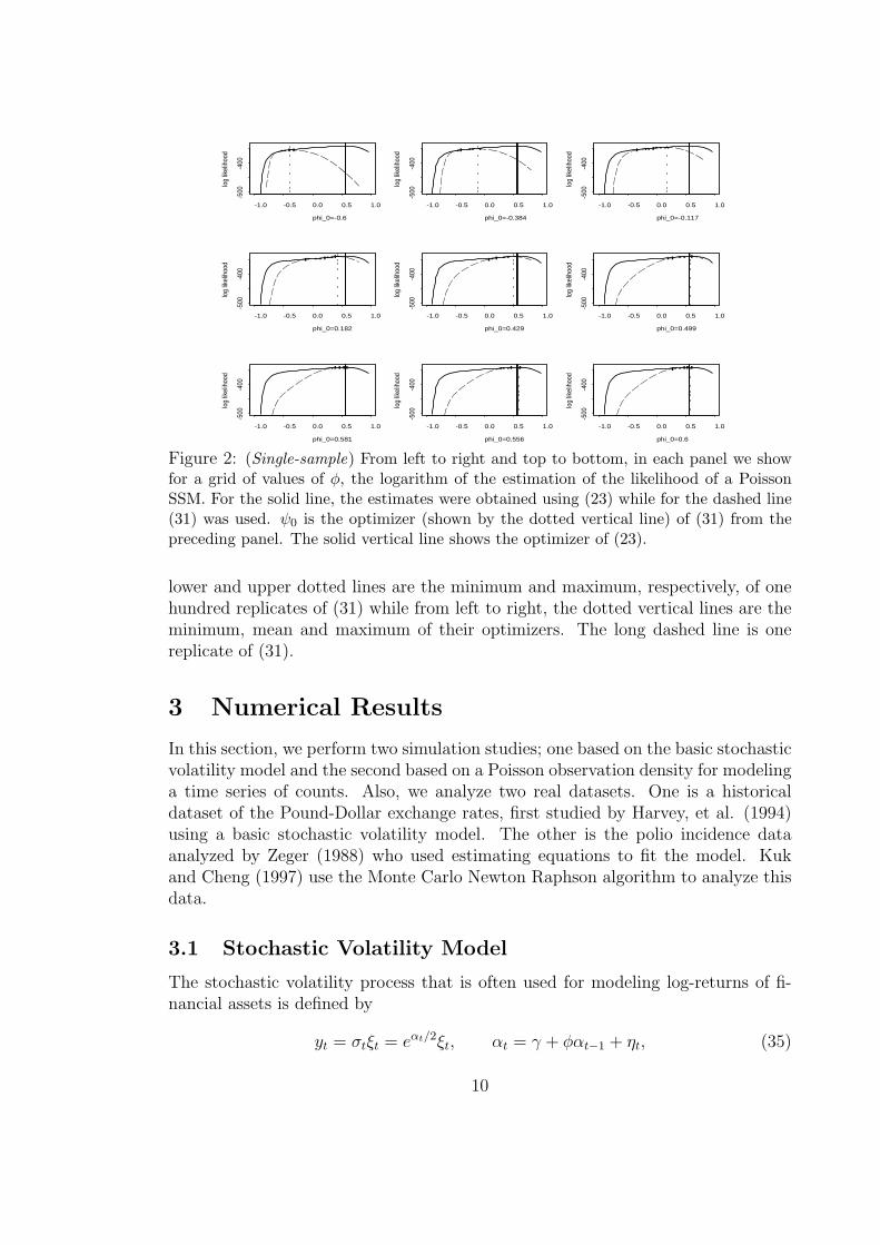
To compute the estimator of the observed likelihood in (31) using the approachdescribed by Kuk (1999), we need an initial value ψ0 and update it to the maximizerof (29) a “few times”. In Figure 2, we use an initial value of φ0 = −0.4, and performsix updatings of this parameter using N = 1000. In each panel of this figure,the solid line is the approximation (23) of the observed likelihood and the thickvertical line shows the maximizer 0.5098 of this function, i.e., the (approximate)ML estimate of φ. In the upper left panel, the long dashed line is the estimationgiven in (31) of the observed likelihood, while the vertical dotted line shows itsmaximizer -0.027. This value is then used as φ0 in the middle panel in the toprow, and so on. As φ0 is updated, the current maximizer of (31) moves “quickly”toward an estimate that is close to the true value. As expected, for given φ0, (31)approximates well the observed likelihood only in a neighborhood of ψ0. Unlike theestimator in (29), the estimator in (31) is smooth, but there is a price to pay forthis gain in terms of imposing a stopping rule. Note that in a vicinity of ψ0, theestimate in (31) is close to the approximate likelihood in (23).

In Figure 3, we show the randomness feature of (31). In each panel, a fixedvalue of φ0 is used. The solid line and vertical solid line are as in Figure 2. The

9

phi_0=-0.6lo

g lik

elih

ood

-1.0 -0.5 0.0 0.5 1.0

-500

-400

phi_0=-0.384

log

likel

ihoo

d

-1.0 -0.5 0.0 0.5 1.0

-500

-400

phi_0=-0.117

log

likel

ihoo

d

-1.0 -0.5 0.0 0.5 1.0

-500

-400

phi_0=0.182

log

likel

ihoo

d

-1.0 -0.5 0.0 0.5 1.0

-500

-400

phi_0=0.429

log

likel

ihoo

d

-1.0 -0.5 0.0 0.5 1.0

-500

-400

phi_0=0.499

log

likel

ihoo

d

-1.0 -0.5 0.0 0.5 1.0

-500

-400

phi_0=0.581

log

likel

ihoo

d

-1.0 -0.5 0.0 0.5 1.0

-500

-400

phi_0=0.556

log

likel

ihoo

d

-1.0 -0.5 0.0 0.5 1.0

-500

-400

phi_0=0.6

log

likel

ihoo

d

-1.0 -0.5 0.0 0.5 1.0

-500

-400

Figure 2: (Single-sample) From left to right and top to bottom, in each panel we showfor a grid of values of φ, the logarithm of the estimation of the likelihood of a PoissonSSM. For the solid line, the estimates were obtained using (23) while for the dashed line(31) was used. ψ0 is the optimizer (shown by the dotted vertical line) of (31) from thepreceding panel. The solid vertical line shows the optimizer of (23).

lower and upper dotted lines are the minimum and maximum, respectively, of onehundred replicates of (31) while from left to right, the dotted vertical lines are theminimum, mean and maximum of their optimizers. The long dashed line is onereplicate of (31).

3 Numerical Results

In this section, we perform two simulation studies; one based on the basic stochasticvolatility model and the second based on a Poisson observation density for modelinga time series of counts. Also, we analyze two real datasets. One is a historicaldataset of the Pound-Dollar exchange rates, first studied by Harvey, et al. (1994)using a basic stochastic volatility model. The other is the polio incidence dataanalyzed by Zeger (1988) who used estimating equations to fit the model. Kukand Cheng (1997) use the Monte Carlo Newton Raphson algorithm to analyze thisdata.

3.1 Stochastic Volatility Model

The stochastic volatility process that is often used for modeling log-returns of fi-nancial assets is defined by

yt = σtξt = eαt/2ξt, αt = γ + φαt−1 + ηt, (35)

10

phi_0=-.5

log

likel

ihoo

d

-0.5 0.0 0.5

-380

-370

-360

-350

-340

phi_0=-0.25

log

likel

ihoo

d

-0.5 0.0 0.5

-380

-370

-360

-350

-340

phi_0=0

log

likel

ihoo

d

-0.5 0.0 0.5

-380

-370

-360

-350

-340

phi_0=0.25

log

likel

ihoo

d

-0.5 0.0 0.5

-380

-370

-360

-350

-340

phi_0=0.50

log

likel

ihoo

d

-0.5 0.0 0.5

-380

-370

-360

-350

-340

phi_0=0.75

log

likel

ihoo

d

-0.5 0.0 0.5

-380

-370

-360

-350

-340

Figure 3: (Single-sample) From left to right and top to bottom, in each panel we showfor a grid of values of φ, the logarithm of the estimation of the likelihood of a PoissonSSM. For the solid line, estimates were obtained using (23). The solid vertical line showsits optimizer. For the dashed line, estimations were obtained using (31) with φ0 shownin the x axis. The dotted lines are the minimum and maximum respectively, of 100replicates using (31). From left to right, the dotted vertical lines are the minimum, meanand maximum of the optimizers of these replicates.

where ξt ∼ iid N(0, 1), ηt ∼ iid N(0, σ2), t = 1, . . . , n = 1000, and |φ| < 1. In thiscase, ψ = (γ, φ, σ2). The format for this simulation study is the same as the layoutconsidered in Jacquier, et al. (1994). They considered nine models, indexed by thecoefficient of variation CV of the conditional variance σ2

t := eαt . For convenience,the parameters of these models are reproduced in Table 1. Jacquier, et al. (1994)point out that the nine models are calibrated so that E(σ2

t ) = 0.0009. Also, fromempirical studies (e.g., Harvey and Shepard, 1993; Jacquier, et al. 1994) values ofφ between 0.9 and 0.98 are of primary interest.

φCV 0.90 0.95 0.9810.0 γ -0.821 -0.4106 -0.1642

σ 0.6750 0.4835 0.3081.0 γ -0.736 -0.368 -0.1472

σ 0.363 0.260 0.16570.1 γ -0.706 -0.353 -0.1412

σ 0.135 0.0964 0.0614

Table 1: Parameter values for a simulation experiment of nine stochastic volatility pro-cesses.

11

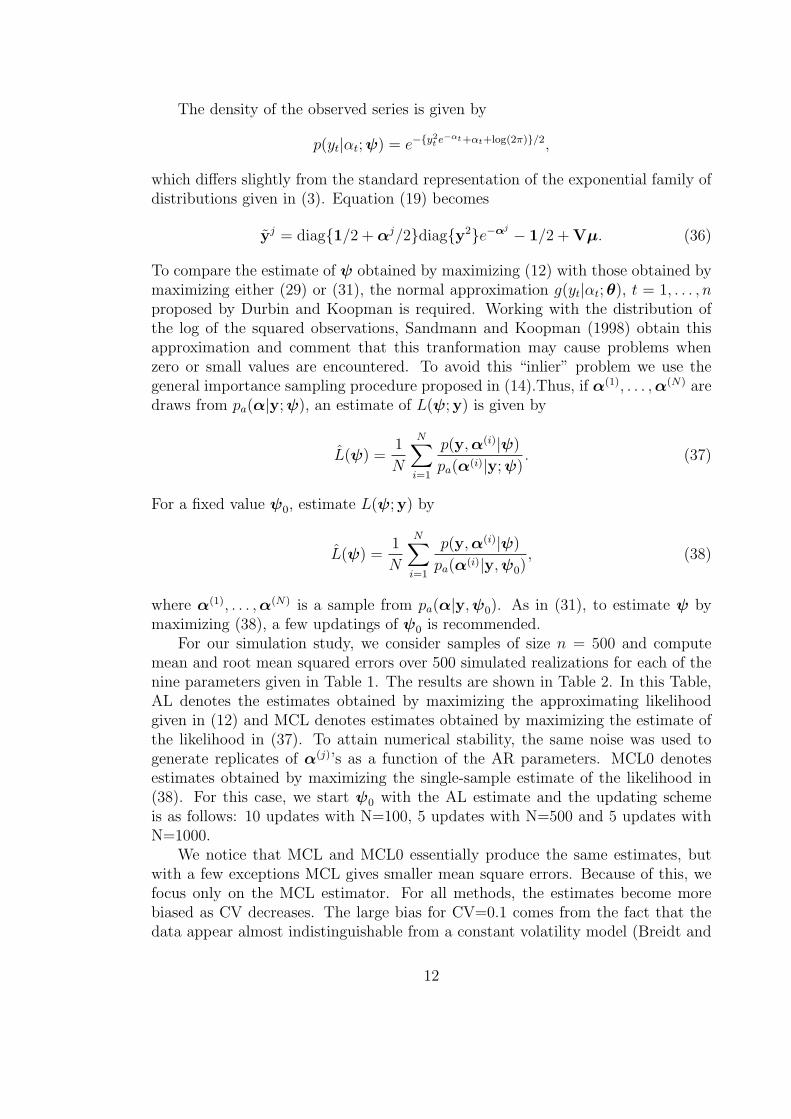
The density of the observed series is given by

p(yt|αt; ψ) = e−{y2t e−αt+αt+log(2π)}/2,

which differs slightly from the standard representation of the exponential family ofdistributions given in (3). Equation (19) becomes

yj = diag{1/2 + αj/2}diag{y2}e−αj − 1/2 + Vµ. (36)

To compare the estimate of ψ obtained by maximizing (12) with those obtained bymaximizing either (29) or (31), the normal approximation g(yt|αt; θ), t = 1, . . . , nproposed by Durbin and Koopman is required. Working with the distribution ofthe log of the squared observations, Sandmann and Koopman (1998) obtain thisapproximation and comment that this tranformation may cause problems whenzero or small values are encountered. To avoid this “inlier” problem we use thegeneral importance sampling procedure proposed in (14).Thus, if α(1), . . . , α(N) aredraws from pa(α|y; ψ), an estimate of L(ψ;y) is given by

L(ψ) =1

N

N∑i=1

p(y,α(i)|ψ)

pa(α(i)|y; ψ). (37)

For a fixed value ψ0, estimate L(ψ;y) by

L(ψ) =1

N

N∑i=1

p(y,α(i)|ψ)

pa(α(i)|y, ψ0), (38)

where α(1), . . . , α(N) is a sample from pa(α|y,ψ0). As in (31), to estimate ψ bymaximizing (38), a few updatings of ψ0 is recommended.

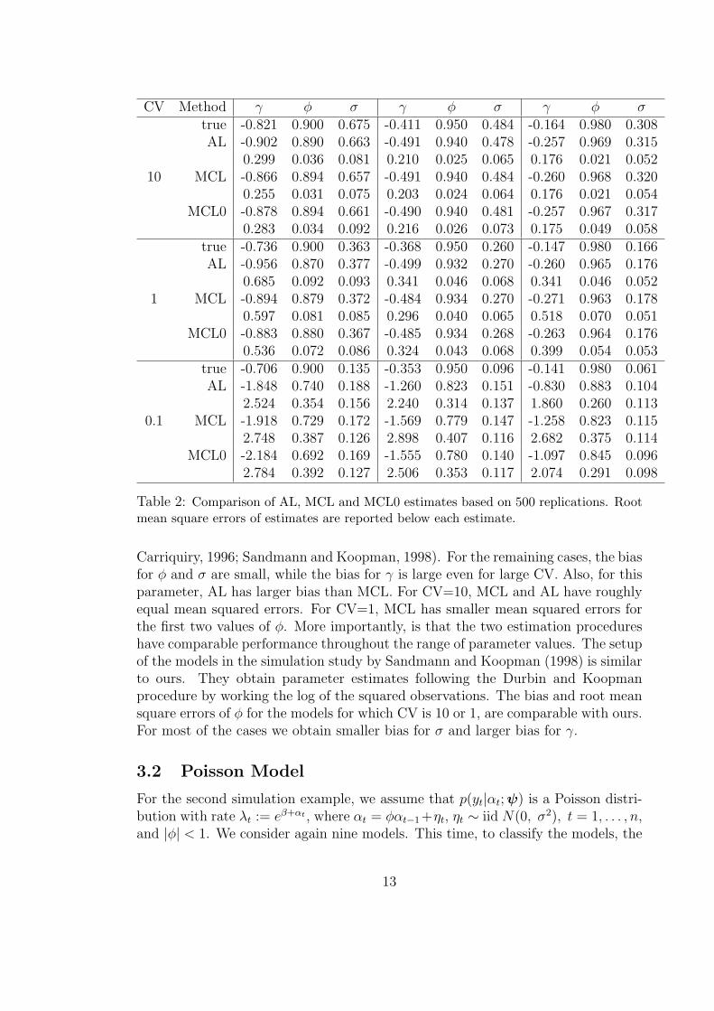
For our simulation study, we consider samples of size n = 500 and computemean and root mean squared errors over 500 simulated realizations for each of thenine parameters given in Table 1. The results are shown in Table 2. In this Table,AL denotes the estimates obtained by maximizing the approximating likelihoodgiven in (12) and MCL denotes estimates obtained by maximizing the estimate ofthe likelihood in (37). To attain numerical stability, the same noise was used togenerate replicates of α(j)’s as a function of the AR parameters. MCL0 denotesestimates obtained by maximizing the single-sample estimate of the likelihood in(38). For this case, we start ψ0 with the AL estimate and the updating schemeis as follows: 10 updates with N=100, 5 updates with N=500 and 5 updates withN=1000.

We notice that MCL and MCL0 essentially produce the same estimates, butwith a few exceptions MCL gives smaller mean square errors. Because of this, wefocus only on the MCL estimator. For all methods, the estimates become morebiased as CV decreases. The large bias for CV=0.1 comes from the fact that thedata appear almost indistinguishable from a constant volatility model (Breidt and

12

CV Method γ φ σ γ φ σ γ φ σtrue -0.821 0.900 0.675 -0.411 0.950 0.484 -0.164 0.980 0.308AL -0.902 0.890 0.663 -0.491 0.940 0.478 -0.257 0.969 0.315

0.299 0.036 0.081 0.210 0.025 0.065 0.176 0.021 0.05210 MCL -0.866 0.894 0.657 -0.491 0.940 0.484 -0.260 0.968 0.320

0.255 0.031 0.075 0.203 0.024 0.064 0.176 0.021 0.054MCL0 -0.878 0.894 0.661 -0.490 0.940 0.481 -0.257 0.967 0.317

0.283 0.034 0.092 0.216 0.026 0.073 0.175 0.049 0.058true -0.736 0.900 0.363 -0.368 0.950 0.260 -0.147 0.980 0.166AL -0.956 0.870 0.377 -0.499 0.932 0.270 -0.260 0.965 0.176

0.685 0.092 0.093 0.341 0.046 0.068 0.341 0.046 0.0521 MCL -0.894 0.879 0.372 -0.484 0.934 0.270 -0.271 0.963 0.178

0.597 0.081 0.085 0.296 0.040 0.065 0.518 0.070 0.051MCL0 -0.883 0.880 0.367 -0.485 0.934 0.268 -0.263 0.964 0.176

0.536 0.072 0.086 0.324 0.043 0.068 0.399 0.054 0.053true -0.706 0.900 0.135 -0.353 0.950 0.096 -0.141 0.980 0.061AL -1.848 0.740 0.188 -1.260 0.823 0.151 -0.830 0.883 0.104

2.524 0.354 0.156 2.240 0.314 0.137 1.860 0.260 0.1130.1 MCL -1.918 0.729 0.172 -1.569 0.779 0.147 -1.258 0.823 0.115

2.748 0.387 0.126 2.898 0.407 0.116 2.682 0.375 0.114MCL0 -2.184 0.692 0.169 -1.555 0.780 0.140 -1.097 0.845 0.096

2.784 0.392 0.127 2.506 0.353 0.117 2.074 0.291 0.098

Table 2: Comparison of AL, MCL and MCL0 estimates based on 500 replications. Rootmean square errors of estimates are reported below each estimate.

Carriquiry, 1996; Sandmann and Koopman, 1998). For the remaining cases, the biasfor φ and σ are small, while the bias for γ is large even for large CV. Also, for thisparameter, AL has larger bias than MCL. For CV=10, MCL and AL have roughlyequal mean squared errors. For CV=1, MCL has smaller mean squared errors forthe first two values of φ. More importantly, is that the two estimation procedureshave comparable performance throughout the range of parameter values. The setupof the models in the simulation study by Sandmann and Koopman (1998) is similarto ours. They obtain parameter estimates following the Durbin and Koopmanprocedure by working the log of the squared observations. The bias and root meansquare errors of φ for the models for which CV is 10 or 1, are comparable with ours.For most of the cases we obtain smaller bias for σ and larger bias for γ.

3.2 Poisson Model

For the second simulation example, we assume that p(yt|αt; ψ) is a Poisson distri-bution with rate λt := eβ+αt , where αt = φαt−1+ηt, ηt ∼ iid N(0, σ2), t = 1, . . . , n,and |φ| < 1. We consider again nine models. This time, to classify the models, the

13

index of dispersion D of the conditional variance of the observations σ2t = eβ+αt

appears to be a more useful characterization of the ability to extract informationin the signal αt than its coefficient of variation. The mean of σ2

t is held fixed at 1.5.The parameters of the models that result with this set up are shown in Table 3.

φD 0.90 0.95 0.98

10.0 β -0.6130 -0.6130 -0.6130σ 0.6221 0.4456 0.2840

1.0 β 0.1501 0.1501 0.1501σ 0.3115 0.2232 0.1422

0.1 β 0.3732 0.3732 0.3732σ 0.1107 0.0793 0.0506

Table 3: Parameter values for a simulation experiment of nine Poisson state-space models.

For this simulation, we consider samples of size n = 500 and compute meanand root mean squared errors over 1000 simulated realizations for each of the nineparameters given in Table 3. The results are shown in Table 4. In this table,AL denotes the estimates obtained by maximizing the approximated likelihoodgiven in (23) and MCL denotes estimates obtained by maximizing the estimate ofthe likelihood in (29). From this table, we notice that the estimates of φ and σ2

deteriorate as D decreases, with large bias for these parameters when D = 0.1.Except for a couple of cases, AL and MCL produce remarkably similar results.

3.3 Bias Correction via Bootstrap

In the two simulation studies that we considered, the approximate MLE of theparameters for the Poisson and stochastic volatility models can be slightly biased.Indeed, we will see in the two applications to real data, that the approximatelikelihood and importance sampling estimates can be very close to each other.Closeness here is “measured” via the Monte Carlo error. In this section, we willshow via simulation that the bias of the estimates can be reduced considerablyusing the bootstrap. Stoffer and Wall, 1991 uses the bootstrap to reduce the biasof the ML estimates of the parameters of a classical Gaussian state-space model.

To implement the bootstrap in our modeling setup, let y1 . . . , yn be observationsfrom a state-space model and let ψAL be the maximizer of the approximate likeli-hood in (12). Following Efron and Tibshirani (1993), the bootstrap bias correctionof the estimate ψAL of ψ is given by

ψAL = ψAL − bias, (39)

where bias = ψ∗−ψAL, and ψ

∗is the average of B bootstrap estimates ψ

∗1, . . . , ψ

∗B.

Here, the bootstrap estimate ψ∗j is the maximizer of the approximate likelihood in

14

D Method β φ σ β φ σ β φ σtrue -0.613 0.900 0.622 -0.613 0.950 0.446 -0.613 0.980 0.284AL -0.593 0.889 0.617 -0.629 0.940 0.444 -0.599 0.969 0.288

10 0.288 0.033 0.061 0.390 0.023 0.055 0.605 0.037 0.061MCL -0.592 0.892 0.614 -0.630 0.941 0.445 -0.600 0.969 0.289

0.287 0.030 0.059 0.390 0.022 0.054 0.603 0.030 0.049true 0.150 0.900 0.312 0.150 0.950 0.223 0.150 0.980 0.142AL 0.152 0.888 0.312 0.143 0.938 0.229 0.142 0.968 0.150

1 0.143 0.039 0.046 0.201 0.028 0.039 0.317 0.030 0.033MCL 0.151 0.889 0.313 0.142 0.938 0.230 0.142 0.968 0.150

0.143 0.037 0.046 0.201 0.027 0.039 0.317 0.022 0.031true 0.373 0.900 0.111 0.373 0.950 0.079 0.373 0.980 0.051AL 0.369 0.759 0.146 0.369 0.868 0.103 0.370 0.873 0.075

0.1 0.064 0.336 0.083 0.081 0.242 0.066 0.114 0.329 0.060MCL 0.371 0.774 0.136 0.369 0.864 0.102 0.370 0.855 0.076

0.063 0.327 0.070 0.080 0.248 0.063 0.114 0.353 0.060

Table 4: Comparison of AL and MCL estimates based on 500 replications. Root meansquare errors of estimates are reported below each estimate.

(12) computed with a realization y∗1 . . . , y∗n drawn from the state-space model thathas true parameters ψAL. The bootstrap estimate of the variance of the estimatorψAL is

var(ψAL) =1

B − 1

B∑j=1

(ψ∗j − ψ

∗)(ψ

∗j − ψ

∗)T . (40)

To assess the performance of the bootstrap bias correction, we conducted asimulation study on three Poisson models with parameters given in the secondrow of Table 3. As seen in Table 4, φ has a moderate bias in these models. Theresults of the simulation are given in Table 5. BC refers to the average of 1000 biascorrected estimates defined in (39) computed with B=100 bootstrap estimates. Thestandard errors of the 1000 bias corrected estimates are also shown in the table.The AL estimates were obtained from 1000 simulated realizations from the state-space model having true parameters given in the second row of Table 3. The rowlabeled AL is the average of the 1000 simulated ψAL estimates. Inspecting thistable, the bootstrap bias correction has done a good job in reducing the bias of theAL estimate of φ with only little alteration of the standard errors.

In Figure 4 we compare the estimated densities of the AL and BC estimatesof the parameters β and φ. Each column in this figure corresponds to the modelswith parameters (0.150, 0.900, 0.312), (0.150, 0.950, 0.223) and (0.150, 0.980, 0.142)respectively. As seen from these graphs, the BC estimates have essentially shiftedthe location of the AL estimates.

15

estimate β φ σ β φ σ β φ σtrue 0.150 0.900 0.312 0.150 0.950 0.223 0.150 0.980 0.142AL 0.153 0.887 0.313 0.147 0.938 0.227 0.140 0.967 0.147

S.E. 0.144 0.038 0.047 0.201 0.026 0.038 0.302 0.029 0.033BC 0.154 0.904 0.305 0.147 0.953 0.217 0.141 0.985 0.133

S.E. 0.144 0.034 0.048 0.202 0.023 0.040 0.303 0.025 0.036

Table 5: Simulation results of bias correction for three Poisson state-space models basedon 1000 replications. The rows labelled AL and BC are the average of the replications.Each AL estimate is the optimizer of the approximate likelihood in (23) and each BCestimate is the bootstrap bias correction estimate defined in (39).

beta

de

nsi

ty

-0.4 0.0 0.2 0.4 0.6 0.8

0.0

0.5

1.0

1.5

2.0

2.5

beta= 0.15

phi

de

nsi

ty

0.70 0.80 0.90

02

46

8

phi= 0.9

beta

de

nsi

ty

-0.5 0.0 0.5 1.0

0.0

0.5

1.0

1.5

beta= 0.15

phi

de

nsi

ty

0.80 0.85 0.90 0.95

05

10

15

phi= 0.95

betad

en

sity

-1.0 -0.5 0.0 0.5 1.0 1.5

0.0

0.2

0.4

0.6

0.8

1.0

1.2

beta= 0.15

phi

de

nsi

ty

0.2 0.4 0.6 0.8 1.0

02

46

phi= 0.98

Figure 4: Parameter densities for β (first row) and φ (second column) for estimationsAL (solid line) and BC (dotted line) for three Poisson state-space models.

3.4 Pound-Dollar Exchange Rates

The first dataset that we analyze is the Pound/Dollar exchange rates. The data,taken from the site http://staff.feweb.vu.nl/koopman/sv/ consists of the log dif-ferences yt of the daily observations of weekdays closing pound to dollar exchangerates zt, t = 1, . . . , 946 from 10/1/81 to 6/28/85. We use the basic stochasticvolatility model (35) to model yt := log(zt) − log(zt−1). Setting the parametervector ψ := (γ, φ, σ2), Table 6 shows various estimates of ψ. The second column,labeled as AL, contains the estimate of ψ obtained by maximizing (12). The col-umn labeled MCL contains the estimate of ψ obtained by maximizing (37). MCE

16

denotes Monte Carlo error and is obtained as the standard error of 1000 estimatesof ψ, using for each estimate the same observations y1, . . . , y945. The standard errorof the estimates AL and MCL are obtained using (40). The columns labeled as BCare bootstrap bias corrections of AL and MCL computed with B = 500 bootstrapestimates. Notice that the AL and MCL estimates are remarkably close. In fact, thedifference between these estimates is due to the randomness of the MCL estimate.For example, two distinct MCL estimates of σ2 are unlikely to differ more than fourtimes the Monte Carlo error, i.e., 0.0028, while the estimates AL and MCE of σ2

differ only by 0.0006. In other words, we would not be able to differentiate the ALestimate from a “cloud” of MCL replicates.

Parameter AL S.E. BC MCL MCE S.E. BCγ -0.0227 0.0198 -0.0140 -0.0230 0.0004 0.0173 -0.0153φ 0.9750 0.0194 0.9845 0.9747 0.0004 0.0166 0.9832

σ2 0.0267 0.0141 0.0228 0.0273 0.0007 0.0138 0.0228

Table 6: Parameter estimates for the Pound-Dollar exchange rates data. AL and MCEare the maximizers of (12) and (37), respectively. BC are bootstrap bias corrected es-timates (B = 500) and S.E. are bootstrap estimates of the standard errors of AL andMCL, respectively. MCE is the standard error of 1000 MCL replicates.

3.5 Polio data

The second dataset consists of the observed time series y1, . . . , y168 of the monthlynumber of U.S. cases of poliomyelitis for 1970 to 1983 that was first considered byZeger (1988). We adopt the same model used by Zeger in which the distribution ofYt, given the state αt, is Poisson with rate λt := eαt+xT

t β. Here, βT := (β1, . . . , β6),xt is the vector of covariates given by

xTt = (1, t/1000, cos(2πt/12), sin(2πt/12), cos(2πt/6), sin(2πt/6)),

and the state process is assumed to follow the AR(1) model given by, αt = φαt−1+ηt,where ηt ∼ iid N(0, σ2), t = 1, . . . , n = 1000, and |φ| < 1. The vector of parametersof this SSM is ψ = (β, φ, σ2). Table 7 contains the results of two estimationprocedures. Columns 2 and 5 labeled as AL and MCL respectively, contain theestimates of ψ obtained by maximizing (12) and (29), respectively. As in theprevious example, MCE denotes Monte Carlo error, based on 1000 replicates of theMCL estimates using for each replicate the same observations y1, . . . , y168.

Notice that only the AL and DK estimates for β2 differ more than the expecteddifference between two DK estimates (4 times MCE). In general the AL estimatesare very close to the DK estimates in spite of the fact that the length n of theobserved time series is not large. We obtain here larger Monte Carlo error thanin Table 6 even when we have used the same number of draws (N = 1000) tocompute the Monte Carlo integration in (37) and (29) respectively. This may not

17

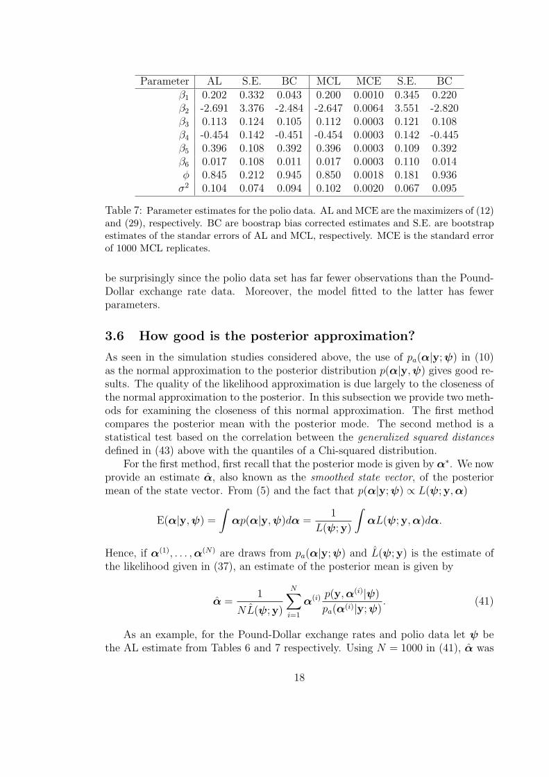
Parameter AL S.E. BC MCL MCE S.E. BCβ1 0.202 0.332 0.043 0.200 0.0010 0.345 0.220β2 -2.691 3.376 -2.484 -2.647 0.0064 3.551 -2.820β3 0.113 0.124 0.105 0.112 0.0003 0.121 0.108β4 -0.454 0.142 -0.451 -0.454 0.0003 0.142 -0.445β5 0.396 0.108 0.392 0.396 0.0003 0.109 0.392β6 0.017 0.108 0.011 0.017 0.0003 0.110 0.014φ 0.845 0.212 0.945 0.850 0.0018 0.181 0.936

σ2 0.104 0.074 0.094 0.102 0.0020 0.067 0.095

Table 7: Parameter estimates for the polio data. AL and MCE are the maximizers of (12)and (29), respectively. BC are boostrap bias corrected estimates and S.E. are bootstrapestimates of the standar errors of AL and MCL, respectively. MCE is the standard errorof 1000 MCL replicates.

be surprisingly since the polio data set has far fewer observations than the Pound-Dollar exchange rate data. Moreover, the model fitted to the latter has fewerparameters.

3.6 How good is the posterior approximation?

As seen in the simulation studies considered above, the use of pa(α|y; ψ) in (10)as the normal approximation to the posterior distribution p(α|y,ψ) gives good re-sults. The quality of the likelihood approximation is due largely to the closeness ofthe normal approximation to the posterior. In this subsection we provide two meth-ods for examining the closeness of this normal approximation. The first methodcompares the posterior mean with the posterior mode. The second method is astatistical test based on the correlation between the generalized squared distancesdefined in (43) above with the quantiles of a Chi-squared distribution.

For the first method, first recall that the posterior mode is given by α∗. We nowprovide an estimate α, also known as the smoothed state vector, of the posteriormean of the state vector. From (5) and the fact that p(α|y; ψ) ∝ L(ψ;y,α)

E(α|y,ψ) =

∫αp(α|y,ψ)dα =

1

L(ψ;y)

∫αL(ψ;y, α)dα.

Hence, if α(1), . . . , α(N) are draws from pa(α|y; ψ) and L(ψ;y) is the estimate ofthe likelihood given in (37), an estimate of the posterior mean is given by

α =1

NL(ψ;y)

N∑i=1

α(i) p(y, α(i)|ψ)

pa(α(i)|y; ψ). (41)

As an example, for the Pound-Dollar exchange rates and polio data let ψ bethe AL estimate from Tables 6 and 7 respectively. Using N = 1000 in (41), α was

18

computed. In Figures 5 and 6 the solid line shows the smoothed state vector, andthe dashed line shows the posterior mode α∗ of p(α|y,ψ) obtained as in (16). Inboth cases, the posterior mode and smoothed state vector are relatively close eventhough the number of observations of the polio data (n=168) is not large. Thisadds support to the goodness of the approximation to the posterior distributionp(α|y; ψ) by a multivariate normal density.

t

smoo

thed

sta

te v

ecto

r

0 200 400 600 800

-2-1

01

Figure 5: (smoothed state vector) For the Pound-Dollar exchange rates data, thesolid line shows estimate of the posterior mean of the state vector and the dashedline shows its posterior mode.

t

smoo

thed

sta

te v

ecto

r

0 50 100 150

-0.5

0.0

0.5

1.0

1.5

Figure 6: (smoothed state vector) For the Polio data, the solid line shows estimateof the posterior mean of the state vector and the dashed line shows its posteriormode.

19

For the second method, if an independent sample from p(α|y,ψ) can be gen-erated, then we could assess the compatibility of the samples with a normal pop-ulation. Such a sample can be obtained as follows: First generate an independentsample α(1),α(2), . . . , α(N) from the approximate distribution pa(α|y,ψ). For Nlarge, an iid sample from the discrete distribution that puts mass pi given by

pi :=wi∑Ni=1 wi

, wi =p(α(i)|y, ψ)

pa(α(i)|y,ψ)∝ L(ψ;y,αi)

pa(α(i)|y,ψ), (42)

is an (approximate) iid sample from p(α|y,ψ). In the Bayesian literature, thismethod is known as sampling importance-resampling (SIR), e.g., Bernardo andSmith (1994). Assume now that α(1), α(2), . . . , α(M) is an iid sample from p(α|y,ψ).If pa(α|y,ψ) in (10) were a good approximation to p(α|y, ψ), for M −n large, thesquared generalized distances

d2j := (α(j) −α∗)T (K∗ + V)(α(j) −α∗), j = 1, . . . , M, (43)

would resemble an iid sample from the chi-squared distribution with n degrees offreedom (Johnson and Wichern, 1998). Thus, a chi-squared QQ-plot of d2

1, . . . , d2M ,

should resemble a straight line through the origin with slope 1.

Observed quantile

chi-sq

ua

re q

ua

ntil

e

30 40 50 60 70 80

30

50

70

n=50, M=100

Observed quantile

chi-sq

ua

re q

ua

ntil

e

30 40 50 60 70 80

30

40

50

60

70

80

n=50, M=100

Observed quantile

chi-sq

ua

re q

ua

ntil

e

30 40 50 60 70 80

30

50

70

n=50, M=100

Observed quantile

chi-sq

ua

re q

ua

ntil

e

80 100 120 140

80

10

01

20

14

0

n=100, M=150

Observed quantile

chi-sq

ua

re q

ua

ntil

e

60 80 100 120 140

60

80

10

01

40

n=100, M=150

Observed quantile

chi-sq

ua

re q

ua

ntil

e

80 100 120 140

80

10

01

20

14

0

n=100, M=150

Observed quantile

chi-sq

ua

re q

ua

ntil

e

160 180 200 220 240 260

16

02

00

24

0

n=200, M=250

Observed quantile

chi-sq

ua

re q

ua

ntil

e

160 180 200 220 240 260

16

02

00

24

0

n=200, M=250

Observed quantile

chi-sq

ua

re q

ua

ntil

e

160 180 200 220 240 260

16

02

00

24

0

n=200, M=250

Figure 7: (Chi-squared QQ-plots) The QQ-plot from i-th row and j-th column wasobtained using a SIR sample α(1), α(2), . . . , α(M) from p(α|y, ψj) by resampling a sampleof size 5000 from the approximation pa(α|y, ψj).

To illustrate this techniques, consider the state-space model for which p(yt|αt; ψ)is the Poisson distribution with rate λt := eβ+αt ; αt = φαt−1 + ηt, ηt ∼ iid

20

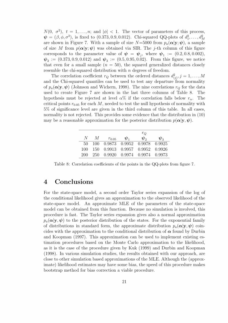
N(0, σ2), t = 1, . . . , n; and |φ| < 1. The vector of parameters of this process,ψ = (β, φ, σ2), is fixed to (0.373, 0.9, 0.012). Chi-squared QQ-plots of d2

1, . . . , d2M

are shown in Figure 7. With a sample of size N=5000 from pa(α|y; ψ), a sampleof size M from p(α|y; ψ) was obtained via SIR. The j-th column of this figurecorresponds to the parameter value of ψ = ψj, where ψ1 := (0.2, 0.8, 0.002),ψ2 := (0.373, 0.9, 0.012) and ψ3 := (0.5, 0.95, 0.02). From this figure, we noticethat even for a small sample (n = 50), the squared generalized distances closelyresemble the chi-squared distribution with n degrees of freedom.

The correlation coefficient rQ between the ordered distances d2(j), j = 1, . . . , M

and the Chi-squared quantiles can be used to test any departure from normalityof pa(α|y,ψ) (Johnson and Wichern, 1998). The nine correlations rQ for the dataused to create Figure 7 are shown in the last three columns of Table 8. Thehypothesis must be rejected at level α% if the correlation falls below rα. Thecritical points r0.05 for each M , needed to test the null hypothesis of normality with5% of significance level are given in the third column of this table. In all cases,normality is not rejected. This provides some evidence that the distribution in (10)may be a reasonable approximation for the posterior distribution p(α|y,ψ).

rQ

N M r0.05 ψ1 ψ2 ψ3

50 100 0.9873 0.9952 0.9978 0.9925100 150 0.9913 0.9957 0.9952 0.9926200 250 0.9920 0.9974 0.9974 0.9973

Table 8: Correlation coefficients of the points in the QQ-plots from figure 7.

4 Conclusions

For the state-space model, a second order Taylor series expansion of the log ofthe conditional likelihood gives an approximation to the observed likelihood of thestate-space model. An approximate MLE of the parameters of the state-spacemodel can be obtained from this function. Because no simulation is involved, thisprocedure is fast. The Taylor series expansion gives also a normal approximationpa(α|y,ψ) to the posterior distribution of the states. For the exponential familyof distributions in standard form, the approximate distribution pa(α|y,ψ) coin-cides with the approximation to the conditional distribution of α found by Durbinand Koopman (1997). This approximation can be used to implement existing es-timation procedures based on the Monte Carlo approximation to the likelihood,as it is the case of the procedure given by Kuk (1999) and Durbin and Koopman(1998). In various simulation studies, the results obtained with our approach, areclose to other simulation based approximations of the MLE. Although the (approx-imate) likelihood estimates may have some bias, the speed of this procedure makesbootstrap method for bias correction a viable procedure.

21

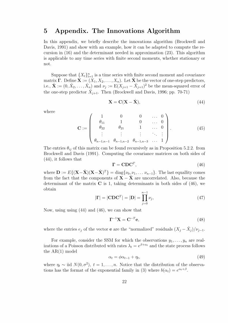
5 Appendix. The Innovations Algorithm

In this appendix, we briefly describe the innovations algorithm (Brockwell andDavis, 1991) and show with an example, how it can be adapted to compute the re-cursion in (16) and the determinant needed in approximation (23). This algorithmis applicable to any time series with finite second moments, whether stationary ornot.

Suppose that {Xt}nt=1 is a time series with finite second moment and covariance

matrix Γ. Define X := (X1, X2, . . . , Xn). Let X be the vector of one-step predictors,i.e., X := (0, X2, . . . , Xn) and νj := E(Xj+1 − Xj+1)

2 be the mean-squared error of

the one-step predictor Xj+1. Then (Brockwell and Davis, 1996; pp. 70-71)

X = C(X− X), (44)

where

C :=

1 0 0 . . . 0θ11 1 0 . . . 0θ22 θ21 1 . . . 0...

......

. . ....

θn−1,n−1 θn−1,n−2 θn−1,n−3 . . . 1

. (45)

The entries θij of this matrix can be found recursively as in Proposition 5.2.2. fromBrockwell and Davis (1991). Computing the covariance matrices on both sides of(44), it follows that

Γ = CDCT , (46)

where D := E{(X−X)(X−X)T} = diag{ν0, ν1, . . . νn−1}. The last equallity comesfrom the fact that the components of X − X are uncorrelated. Also, because thedeterminant of the matrix C is 1, taking determinants in both sides of (46), weobtain

|Γ| = |CDCT | = |D| =n−1∏j=0

νj, (47)

Now, using using (44) and (46), we can show that

Γ−1X = C−Te, (48)

where the entries ej of the vector e are the “normalized” residuals (Xj − Xj)/νj−1.

For example, consider the SSM for which the observations y1, . . . , yn are real-izations of a Poisson distributed with rates λt = eβ+αt and the state process followsthe AR(1) model

αt = φαt−1 + ηt, (49)

where ηt ∼ iid N(0, σ2), t = 1, . . . , n. Notice that the distribution of the observa-tions has the format of the exponential family in (3) where b(αt) = eαt+β.

22

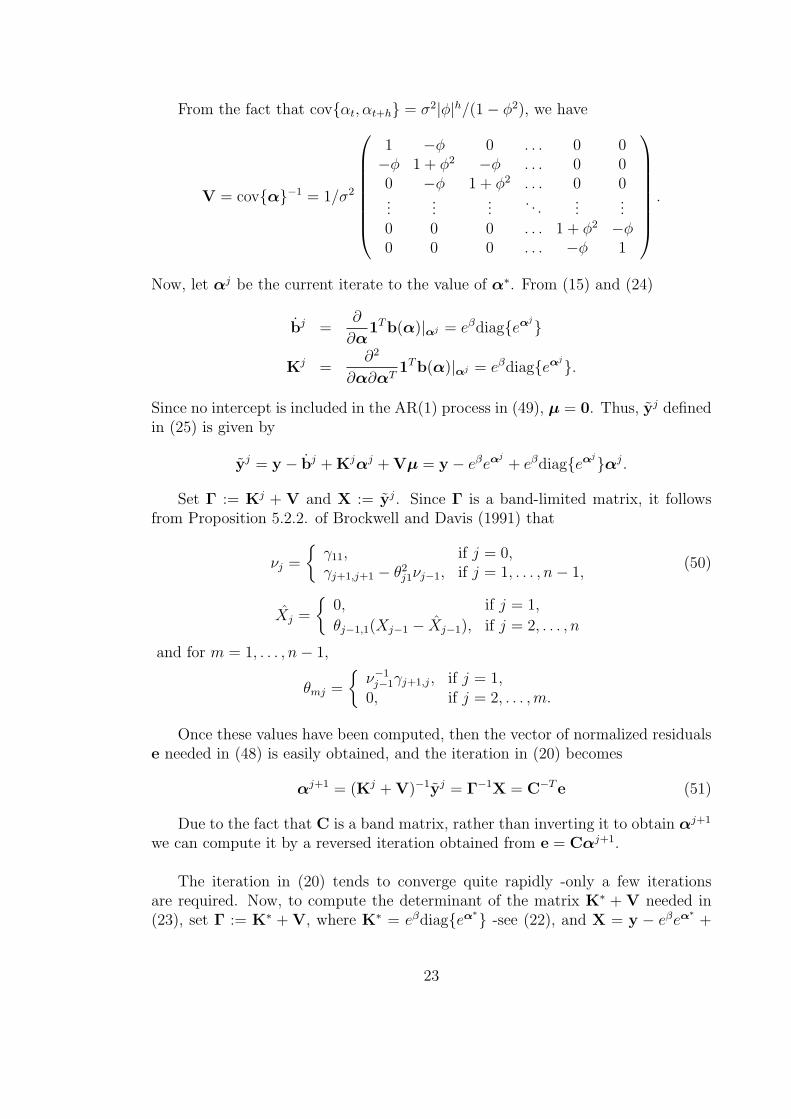
From the fact that cov{αt, αt+h} = σ2|φ|h/(1− φ2), we have

V = cov{α}−1 = 1/σ2

1 −φ 0 . . . 0 0−φ 1 + φ2 −φ . . . 0 00 −φ 1 + φ2 . . . 0 0...

......

. . ....

...0 0 0 . . . 1 + φ2 −φ0 0 0 . . . −φ 1

.

Now, let αj be the current iterate to the value of α∗. From (15) and (24)

bj =∂

∂α1Tb(α)|αj = eβdiag{eαj}

Kj =∂2

∂α∂αT1Tb(α)|αj = eβdiag{eαj}.

Since no intercept is included in the AR(1) process in (49), µ = 0. Thus, yj definedin (25) is given by

yj = y − bj + Kjαj + Vµ = y − eβeαj

+ eβdiag{eαj}αj.

Set Γ := Kj + V and X := yj. Since Γ is a band-limited matrix, it followsfrom Proposition 5.2.2. of Brockwell and Davis (1991) that

νj =

{γ11, if j = 0,γj+1,j+1 − θ2

j1νj−1, if j = 1, . . . , n− 1,(50)

Xj =

{0, if j = 1,

θj−1,1(Xj−1 − Xj−1), if j = 2, . . . , n

and for m = 1, . . . , n− 1,

θmj =

{ν−1

j−1γj+1,j, if j = 1,0, if j = 2, . . . , m.

Once these values have been computed, then the vector of normalized residualse needed in (48) is easily obtained, and the iteration in (20) becomes

αj+1 = (Kj + V)−1yj = Γ−1X = C−Te (51)

Due to the fact that C is a band matrix, rather than inverting it to obtain αj+1

we can compute it by a reversed iteration obtained from e = Cαj+1.

The iteration in (20) tends to converge quite rapidly -only a few iterationsare required. Now, to compute the determinant of the matrix K∗ + V needed in(23), set Γ := K∗ + V, where K∗ = eβdiag{eα∗} -see (22), and X = y − eβeα∗ +

23

eβdiag{eα∗}α∗, where α∗ is the converged value of the iteration in (51). Then,from (47),

|K∗ + V| = |Γ| =n−1∏j=0

νj,

where νj, j = 0, . . . , n − 1 must be computed as in (50). Extensions to state pro-cesses following an AR(p) model can be handled in a similar fashion.

Acknowledgments

This research was supported in part by NSF grant DMS-0308109 and EPA STARCR-829095, and a scholarship from Consejo Nacional de Ciencia y Tecnologia(CONACYT). The authors also wish thank W.T.M Dunsmuir for his commentsand helpful suggestions.

References

[1] Bernardo, J. M. and Smith, A. F. M (1994). “Bayesian Theory” J. Wiley, NewYork.

[2] Breidt, F. J. and Carriquiry, A. L. (1996). “Improved Quasi-Maximum Likeli-hood Estimation for Stochastic Volatility Models.” In: Zellner, A., Lee, J. S.(Eds.), Modeling and Prediction: Honouring Seymour Geisser. Springer, NewYork.

[3] Brockwell, P. J. and Davis, R. A. (1991). “Time Series: Theory and Methods.”(2nd ed.) Springer-Verlag, New York.

[4] Brockwell, P. J. and Davis, R. A. (1996). “Introduction to Time Series andForecasting.” Springer-Verlag, New York.

[5] Campbell, M. J. (1994) “Time Series Regression for Counts: an InvestigationInto the Relationship Between Sudden Infant Death Syndrome and Environ-mental Temperature.” J. R. Stat. Soc. Ser. A, 157, 191-208.

[6] Chan, K. S. and Ledolter, J. (1995). “Monte Carlo EM Estimation for TimeSeries Models Involving Counts.” J. Amer. Statist. Assoc., 90, 242-252.

[7] Davis, R. A., Dunsmuir, W. T. M. and Wang, Y. (1988). “Modelling TimeSeries of Count Data.” In Asymptotics, Nonparametrics and Time Series (edSubir Ghosh), Marcel Dekker.

[8] Durbin, J. and Koopman, S. J. (1997) “Monte Carlo Maximum LikelihoodEstimation for non-Gaussian State Space Models.” Biometrika, 84, 669-684.

24

[9] Durbin, J. and Koopman, S. J. (2001) “Time Series Analysis by State SpaceMethods.” Oxford, NY.

[10] Efron, B. and Tibshirani R. J. (1993) “An Introduction to the Bootstrap.”Chapman and Hall, NY.

[11] Geyer, C. J. (1996) “Estimation and optimization of functions.” In MarkovChain Monte Carlo in Practice (eds W. R. Gilks, S. Richardson and D. J.Spiegelhalter), Chapman & Hall, London, pp. 89-114.

[12] Geweke, J. and Tanizaki, H. (1999) “On Markov Chain Monte Carlo Methodsfor Nonlinear and Non-Gaussian State-Space Models.” Comm. Statist. Simula-tion Comput., 28, 867-894.

[13] Harvey, A. C. (1989) “Forecasting, Structural Time Series Models and theKalman Filter.” Cambridge: Cambridge University Press.

[14] Harvey, A. C. and Fernandes, C. (1989) “Time Series Models for Count orQualitative Observations.” J. Amer. Statist. Assoc., 7, 407-417.

[15] Harvey, A. C. and Streibel, M. (1998) “Testing for a slowly changing level withspecial reference to stochastic volatility.” J. Econometrics, 87, 167-189.

[16] Harvey, A. C. and Shepard, N. (1993) “Estimation and Testing of StochasticVariance Models.” Unpublished manuscript, The London School of Economics.

[17] Harvey, A. C., Ruiz, E. and Shepard, N. (1994) “Multivariate Stochastic Vari-ance Models.” Rev. Econom. Stud., 61, 247-264.

[18] Jacquier, E., Polson, N. G. and Rossi, P. E. (1994) “Bayesian analysis ofstochastic volatility models (with discussion).” J. Bus. Econom. Statist., 12,371-417.

[19] Kuk, A. Y. (1999) “The Use of Approximating Models in Monte Carlo Maxi-mum Likelihood Estimation.” Statist. Probab. Lett., 45, 325-333.

[20] Kuk, A. Y. and Cheng, Y. W. (1997) “The Monte Carlo Newton-RaphsonAlgorithm.” J. Stat. Comput. Simul., 59, 233-250.

[21] Pitt, M. K and Shepard N. (1999). “Filtering via Simulation: Auxiliary ParticleFilters.” J. Amer. Statist. Assoc., 94, 590-599.

[22] Sandmann, G. and Koopman, S. J. (1998) “Estimation of Stochastic VolatilityModels via Monte Carlo Maximum Likelihood.” J. Econometrics, 87, 271-301.

[23] Stoffer, D. S. and Wall, K. D. (1991) “Bootstrapping State-Space Models:Gaussian Maximum Likelihood and the Kalman Filter.” J. Amer. Statist. As-soc., 86, 1024-1032.

25

[24] Wichern, W. and Johnson, R. A. (1998) “Applied Multivariate Statistical Anal-ysis.” (Fourth ed.) Prentice Hall, New Jersey.

[25] Zeger, S. L. (1988) “A Regresion Model for Time Series of Counts.” Biometrika,75, 621-629.

26