Estimation and Control over Communication Networks
540
Transcript of Estimation and Control over Communication Networks


Control Engineering
Series EditorWilliam S. LevineDepartment of Electrical and Computer EngineeringUniversity of MarylandCollege Park, MD 20742-3285USA
Editorial Advisory BoardOkko BosgraDelft UniversityThe Netherlands
Graham GoodwinUniversity of NewcastleAustralia
Petar KokotovicUniversity of CaliforniaSanta BarbaraUSA
Manfred MorariETHZürichSwitzerland
William PowersFord Motor Company (retired)USA
Mark SpongUniversity of IllinoisUrbana-ChampaignUSA
Iori HashimotoKyoto UniversityKyotoJapan

Alexey S. MatveevAndrey V. Savkin
Estimation and Control overCommunication Networks
BirkhäuserBoston • Basel • Berlin

Alexey S. MatveevDepartment of Mathematics
and MechanicsSaint Petersburg University198504 PetrodovoretzSaint PetersburgRussia
Andrey V. SavkinSchool of Electrical Engineering
and TelecommunicationsUniversity of New South WalesNSW2052 SydneyAustralia
ISBN: 978-0-8176-4494-9 e-ISBN: 978-0-8176-4607-3DOI: 10.1007/978-0-8176-4067-3
Library of Congress Control Number: 2008929989
© +Business Media, LLCAll rights reserved. This work may not be translated or copied in whole or in part without the writ-ten permission of the publisher (Birkhäuser Boston, c/o Springer Science+Business Media, LLC,233 Spring Street, New York, NY 10013, USA), except for brief excerpts in connection with reviewsor scholarly analysis. Use in connection with any form of information storage and retrieval, electronicadaptation, computer software, or by similar or dissimilar methodology now known or hereafter de-veloped is forbidden.The use in this publication of trade names, trademarks, service marks, and similar terms, even if theyare not identified as such, is not to be taken as an expression of opinion as to whether or not they aresubject to proprietary rights.
Printed on acid-free paper.
9 8 7 6 5 4 3 2 1
www.birkhauser.com
2009 Birkhäuser Boston, a part of Springer Science

Preface
Rapid advances in communication technology have opened up the possibility oflarge-scale control systems in which the control task is distributed among severalprocessors and the communication among the processors, sensors, and actuators isvia communication channels. Such control systems may be distributed over large dis-tances and may use large numbers of actuators and sensors. The possibility of suchnetworked control systems motivates the development of a new chapter of controltheory in which control and communication issues are integrated, and all the limita-tions of communication channels are taken into account. There is an emerging litera-ture on this topic; however, at present there is no systematic theory of estimation andcontrol over communication networks. This book is concerned with the developmentof such a theory.
This book is primarily a research monograph that presents, in a unified man-ner, some recent research on control and estimation over communication channels.It is essentially self-contained and is intended both for researchers and advancedpostgraduate students working in the areas of control engineering, communications,information theory, signal processing or applied mathematics with an interest in theemerging field of networked control systems. The reader is assumed to be competentin the basic mathematical techniques of modern control theory.
By restricting ourselves to several selected problems of estimation and controlover communication networks, we are able to present and prove a number of resultsconcerning optimality, stability, and robustness that are of practical significance fornetworked control system design. In particular, various problems of Kalman filtering,stabilization, and optimal control over communication channels are considered andsolved. The results establish fundamental links among mathematical control theory,Shannon information theory, and entropy theory of dynamical systems. We hopethat the reader finds this work both useful and interesting and is inspired to explorefurther the diverse and challenging area of networked control systems. This book isone of the first research monographs on estimation and control over communicationnetworks.
The material presented in this book derives from a period of fruitful research col-laboration between the authors on the area of networked control systems beginning

vi Preface
in 1999 and is still ongoing. Some of the material contained herein has appeared asisolated results in journal papers and conference proceedings. This work presentsthis material in an integrated and coherent manner and presents many new results.Much of the material arose from joint work with students and colleagues, and the au-thors wish to acknowledge the major contributions made by Veerachai Malyavej, IanPetersen, Rob Evans, Teddy Cheng, Efstratios Skafidas, and Valery Ugrinovskii. Ourthanks for the help with some figures in the book go to Teddy Cheng and VeerachaiMalyavej. We are also grateful to our colleagues Girish Nair, Daniel Liberzon, Vic-tor Solo, Tamer Basar, David Clements, and Andrey Barabanov who have provideduseful comments and suggestions.
The authors wish to acknowledge the support they have received throughout thepreparation of this work from the School of Electrical Engineering and Telecommu-nications at the University of New South Wales, Sydney, and the Faculty of Math-ematics and Mechanics at the Saint Petersburg University. The authors are also ex-tremely grateful for the financial support they have received from the Australian Re-search Council, the Russian Foundation for Basic Research (grant 06-08-01386), andthe Research Council of the President of the Russian Federation (grant 2387.2008.1).
Furthermore, the first author is grateful for the enormous support he has receivedfrom his wife Elena and daughter Julia. Also, the second author is indebted to theendless love and support he has received from his wife Natalia and children Mikhailand Katerina.
Alexey S. Matveev Saint Petersburg, RussiaAndrey V. Savkin Sydney, Australia
March 2008

Contents
Preface . . . . . . . . . . . . . . . . . . . . . . . . . . . . . . . . . . . . . . . . . . . . . . . . . . . . . . . v
1 Introduction . . . . . . . . . . . . . . . . . . . . . . . . . . . . . . . . . . . . . . . . . . . . . . . . . . . 11.1 Control Systems and Communication Networks . . . . . . . . . . . . . . . . . 11.2 Overview of the Book . . . . . . . . . . . . . . . . . . . . . . . . . . . . . . . . . . . . . . . 3
1.2.1 Estimation and Control over Limited CapacityDeterministic Channels . . . . . . . . . . . . . . . . . . . . . . . . . . . . . . . 3
1.2.2 An Analog of Shannon Information Theory: Estimationand Control over Noisy Discrete Channels . . . . . . . . . . . . . . . 5
1.2.3 Decentralized Stabilization via Limited CapacityCommunication Networks . . . . . . . . . . . . . . . . . . . . . . . . . . . . . 6
1.2.4 H∞ State Estimation via Communication Channels . . . . . . . 61.2.5 Kalman Filtering and Optimal Control via Asynchronous
Channels with Irregular Delays . . . . . . . . . . . . . . . . . . . . . . . . . 71.2.6 Kalman Filtering with Switched Sensors . . . . . . . . . . . . . . . . . 71.2.7 Some Other Remarks . . . . . . . . . . . . . . . . . . . . . . . . . . . . . . . . . 8
1.3 Frequently Used Notations . . . . . . . . . . . . . . . . . . . . . . . . . . . . . . . . . . . 8
2 Topological Entropy, Observability, Robustness, Stabilizability, andOptimal Control . . . . . . . . . . . . . . . . . . . . . . . . . . . . . . . . . . . . . . . . . . . . . . . 132.1 Introduction . . . . . . . . . . . . . . . . . . . . . . . . . . . . . . . . . . . . . . . . . . . . . . . 132.2 Observability via Communication Channels . . . . . . . . . . . . . . . . . . . . 142.3 Topological Entropy and Observability of Uncertain Systems . . . . . . 152.4 The Case of Linear Systems . . . . . . . . . . . . . . . . . . . . . . . . . . . . . . . . . . 212.5 Stabilization via Communication Channels . . . . . . . . . . . . . . . . . . . . . 242.6 Optimal Control via Communication Channels . . . . . . . . . . . . . . . . . . 262.7 Proofs of Lemma 2.4.3 and Theorems 2.5.3 and 2.6.4 . . . . . . . . . . . . 28
3 Stabilization of Linear Multiple Sensor Systems via LimitedCapacity Communication Channels . . . . . . . . . . . . . . . . . . . . . . . . . . . . . . 373.1 Introduction . . . . . . . . . . . . . . . . . . . . . . . . . . . . . . . . . . . . . . . . . . . . . . . 37

viii Contents
3.2 Example . . . . . . . . . . . . . . . . . . . . . . . . . . . . . . . . . . . . . . . . . . . . . . . . . . 393.3 General Problem Statement . . . . . . . . . . . . . . . . . . . . . . . . . . . . . . . . . . 413.4 Basic Definitions and Assumptions . . . . . . . . . . . . . . . . . . . . . . . . . . . . 42
3.4.1 Transmission Capacity of the Channel . . . . . . . . . . . . . . . . . . . 423.4.2 Examples . . . . . . . . . . . . . . . . . . . . . . . . . . . . . . . . . . . . . . . . . . . 443.4.3 Stabilizable Multiple Sensor Systems . . . . . . . . . . . . . . . . . . . 453.4.4 Recursive Semirational Controllers . . . . . . . . . . . . . . . . . . . . . 463.4.5 Assumptions about the System (3.3.1), (3.3.2) . . . . . . . . . . . . 49
3.5 Main Result . . . . . . . . . . . . . . . . . . . . . . . . . . . . . . . . . . . . . . . . . . . . . . . 513.5.1 Some Consequences from the Main Result . . . . . . . . . . . . . . . 553.5.2 Complement to the Sufficient Conditions . . . . . . . . . . . . . . . . 553.5.3 Complements to the Necessary Conditions . . . . . . . . . . . . . . . 56
3.6 Application of the Main Result to the Example from Sect. 3.2 . . . . . 573.7 Necessary Conditions for Stabilizability . . . . . . . . . . . . . . . . . . . . . . . . 59
3.7.1 An Extension of the Claim (i) from Theorem 2.5.3 (on p. 26) 593.7.2 An Auxiliary Subsystem . . . . . . . . . . . . . . . . . . . . . . . . . . . . . . 603.7.3 Stabilizability of the Auxiliary Subsystem . . . . . . . . . . . . . . . 613.7.4 Proof of the Necessity Part (i)⇒ (ii) of Theorem 3.5.2 . . . . . 62
3.8 Sufficient Conditions for Stabilizability . . . . . . . . . . . . . . . . . . . . . . . . 623.8.1 Some Ideas Underlying the Design of the Stabilizing
Controller . . . . . . . . . . . . . . . . . . . . . . . . . . . . . . . . . . . . . . . . . . 633.8.2 Plan of Proving the Sufficiency Part of Theorem 3.5.2 . . . . . 653.8.3 Decomposition of the System . . . . . . . . . . . . . . . . . . . . . . . . . . 663.8.4 Separate Stabilization of Subsystems . . . . . . . . . . . . . . . . . . . . 683.8.5 Contracted Quantizer with the Nearly Minimal Number of
Levels . . . . . . . . . . . . . . . . . . . . . . . . . . . . . . . . . . . . . . . . . . . . . 773.8.6 Construction of a Deadbeat Stabilizer . . . . . . . . . . . . . . . . . . . 803.8.7 Stabilization of the Entire System . . . . . . . . . . . . . . . . . . . . . . 813.8.8 Analysis of Assumptions A1) and A2) on p. 81 . . . . . . . . . . . 833.8.9 Inconstructive Sufficient Conditions for Stabilizability . . . . . 853.8.10 Convex Duality and a Criterion for the System (3.8.34) to
be Solvable . . . . . . . . . . . . . . . . . . . . . . . . . . . . . . . . . . . . . . . . . 863.8.11 Proof of the Sufficiency Part of Theorem 3.5.2 for Systems
with Both Unstable and Stable Modes . . . . . . . . . . . . . . . . . . . 883.8.12 Completion of the Proof of Theorem 3.5.2 and the Proofs
of Propositions 3.5.4 and 3.5.8 . . . . . . . . . . . . . . . . . . . . . . . . . 893.9 Comments on Assumption 3.4.24 . . . . . . . . . . . . . . . . . . . . . . . . . . . . . 90
3.9.1 Counterexample . . . . . . . . . . . . . . . . . . . . . . . . . . . . . . . . . . . . . 913.9.2 Stabilizability of the System (3.9.2) . . . . . . . . . . . . . . . . . . . . . 93
4 Detectability and Output Feedback Stabilizability of NonlinearSystems via Limited Capacity Communication Channels . . . . . . . . . . . 1014.1 Introduction . . . . . . . . . . . . . . . . . . . . . . . . . . . . . . . . . . . . . . . . . . . . . . . 1014.2 Detectability via Communication Channels . . . . . . . . . . . . . . . . . . . . . 102
4.2.1 Preliminary Lemmas . . . . . . . . . . . . . . . . . . . . . . . . . . . . . . . . . 103

Contents ix
4.2.2 Uniform State Quantization . . . . . . . . . . . . . . . . . . . . . . . . . . . . 1054.3 Stabilization via Communication Channels . . . . . . . . . . . . . . . . . . . . . 1084.4 Illustrative Example . . . . . . . . . . . . . . . . . . . . . . . . . . . . . . . . . . . . . . . . 111
5 Robust Set-Valued State Estimation via Limited CapacityCommunication Channels . . . . . . . . . . . . . . . . . . . . . . . . . . . . . . . . . . . . . . . 1155.1 Introduction . . . . . . . . . . . . . . . . . . . . . . . . . . . . . . . . . . . . . . . . . . . . . . . 1155.2 Uncertain Systems . . . . . . . . . . . . . . . . . . . . . . . . . . . . . . . . . . . . . . . . . . 116
5.2.1 Uncertain Systems with Integral Quadratic Constraints . . . . . 1165.2.2 Uncertain Systems with Norm-Bounded Uncertainty . . . . . . 1175.2.3 Sector-Bounded Nonlinearities . . . . . . . . . . . . . . . . . . . . . . . . . 118
5.3 State Estimation Problem . . . . . . . . . . . . . . . . . . . . . . . . . . . . . . . . . . . . 1195.4 Optimal Coder–Decoder Pair . . . . . . . . . . . . . . . . . . . . . . . . . . . . . . . . . 1225.5 Suboptimal Coder–Decoder Pair . . . . . . . . . . . . . . . . . . . . . . . . . . . . . . 1235.6 Proofs of Lemmas 5.3.2 and 5.4.2 . . . . . . . . . . . . . . . . . . . . . . . . . . . . . 126
6 An Analog of Shannon Information Theory: State Estimation andStabilization of Linear Noiseless Plants via Noisy Discrete Channels . 1316.1 Introduction . . . . . . . . . . . . . . . . . . . . . . . . . . . . . . . . . . . . . . . . . . . . . . . 1316.2 State Estimation Problem . . . . . . . . . . . . . . . . . . . . . . . . . . . . . . . . . . . . 1346.3 Assumptions, Notations, and Basic Definitions . . . . . . . . . . . . . . . . . . 136
6.3.1 Assumptions . . . . . . . . . . . . . . . . . . . . . . . . . . . . . . . . . . . . . . . . 1366.3.2 Average Mutual Information . . . . . . . . . . . . . . . . . . . . . . . . . . . 1376.3.3 Capacity of a Discrete Memoryless Channel . . . . . . . . . . . . . . 1386.3.4 Recursive Semirational Observers . . . . . . . . . . . . . . . . . . . . . . 139
6.4 Conditions for Observability of Noiseless Linear Plants . . . . . . . . . . 1406.5 Stabilization Problem . . . . . . . . . . . . . . . . . . . . . . . . . . . . . . . . . . . . . . . 1436.6 Conditions for Stabilizability of Noiseless Linear Plants . . . . . . . . . . 145
6.6.1 The Domain of Stabilizability Is Determined by theShannon Channel Capacity . . . . . . . . . . . . . . . . . . . . . . . . . . . . 145
6.7 Necessary Conditions for Observability and Stabilizability . . . . . . . . 1476.7.1 Proposition 6.7.2 Follows from Proposition 6.7.1 . . . . . . . . . . 1486.7.2 Relationship between the Statements (i) and (ii) of
Proposition 6.7.1 . . . . . . . . . . . . . . . . . . . . . . . . . . . . . . . . . . . . . 1496.7.3 Differential Entropy of a Random Vector and Joint Entropy
of a Random Vector and Discrete Quantity . . . . . . . . . . . . . . . 1506.7.4 Probability of Large Estimation Errors . . . . . . . . . . . . . . . . . . 1526.7.5 Proof of Proposition 6.7.1 under Assumption 6.7.11 . . . . . . . 1556.7.6 Completion of the Proofs of Propositions 6.7.1 and 6.7.2:
Dropping Assumption 6.7.11 . . . . . . . . . . . . . . . . . . . . . . . . . . 1566.8 Tracking with as Large a Probability as Desired: Proof of the
c > H(A)⇒ b) Part of Theorem 6.4.1 . . . . . . . . . . . . . . . . . . . . . . . . . 1606.8.1 Error Exponents for Discrete Memoryless Channels . . . . . . . 1616.8.2 Coder–Decoder Pair without a Communication Feedback . . 162

x Contents
6.8.3 Tracking with as Large a Probability as Desired without aCommunication Feedback . . . . . . . . . . . . . . . . . . . . . . . . . . . . . 165
6.9 Tracking Almost Surely by Means of Fixed-Length Code Words:Proof of the c > H(A)⇒ a) part of Theorem 6.4.1 . . . . . . . . . . . . . . 1686.9.1 Coder–Decoder Pair with a Communication Feedback . . . . . 1686.9.2 Tracking Almost Surely by Means of Fixed-Length Code
Words . . . . . . . . . . . . . . . . . . . . . . . . . . . . . . . . . . . . . . . . . . . . . . 1706.9.3 Proof of Proposition 6.9.8 . . . . . . . . . . . . . . . . . . . . . . . . . . . . . 171
6.10 Completion of the Proof of Theorem 6.4.1 (on p. 140): DroppingAssumption 6.8.1 (on p. 161) . . . . . . . . . . . . . . . . . . . . . . . . . . . . . . . . . 179
6.11 Stabilizing Controller and the Proof of the Sufficient Conditionsfor Stabilizability . . . . . . . . . . . . . . . . . . . . . . . . . . . . . . . . . . . . . . . . . . . 1796.11.1 Almost Sure Stabilization by Means of Fixed-Length Code
Words and Low-Rate Feedback Communication . . . . . . . . . . 1806.11.2 Almost Sure Stabilization by Means of Fixed-Length
Code Words in the Absence of a Special FeedbackCommunication Link . . . . . . . . . . . . . . . . . . . . . . . . . . . . . . . . . 185
6.11.3 Proof of Proposition 6.11.22 . . . . . . . . . . . . . . . . . . . . . . . . . . . 1886.11.4 Completion of the Proof of Theorem 6.6.1 . . . . . . . . . . . . . . . 196
7 An Analog of Shannon Information Theory: State Estimation andStabilization of Linear Noisy Plants via Noisy Discrete Channels . . . . 1997.1 Introduction . . . . . . . . . . . . . . . . . . . . . . . . . . . . . . . . . . . . . . . . . . . . . . . 1997.2 Problem of State Estimation in the Face of System Noises . . . . . . . . 2027.3 Zero Error Capacity of the Channel . . . . . . . . . . . . . . . . . . . . . . . . . . . 2037.4 Conditions for Almost Sure Observability of Noisy Plants . . . . . . . . 2067.5 Almost Sure Stabilization in the Face of System Noises . . . . . . . . . . 2087.6 Necessary Conditions for Observability and Stabilizability: Proofs
of Theorem 7.4.1 and i) of Theorem 7.5.3 . . . . . . . . . . . . . . . . . . . . . . 2117.6.1 Proof of i) in Proposition 7.6.2 for Erasure Channels . . . . . . . 2117.6.2 Preliminaries . . . . . . . . . . . . . . . . . . . . . . . . . . . . . . . . . . . . . . . . 2147.6.3 Block Codes Fabricated from the Observer . . . . . . . . . . . . . . . 2187.6.4 Errorless Block Code Hidden within a Tracking Observer . . 2207.6.5 Completion of the Proofs of Proposition 7.6.2,
Theorem 7.4.1, and i) of Theorem 7.5.3 . . . . . . . . . . . . . . . . . 2237.7 Almost Sure State Estimation in the Face of System Noises: Proof
of Theorem 7.4.5 . . . . . . . . . . . . . . . . . . . . . . . . . . . . . . . . . . . . . . . . . . . 2237.7.1 Construction of the Coder and Decoder-Estimator . . . . . . . . . 2237.7.2 Almost Sure State Estimation in the Face of System Noises . 2277.7.3 Completion of the Proof of Theorem 7.4.5 . . . . . . . . . . . . . . . 232
7.8 Almost Sure Stabilization in the Face of System Noises: Proof of(ii) from Theorem 7.5.3 . . . . . . . . . . . . . . . . . . . . . . . . . . . . . . . . . . . . . 2337.8.1 Feedback Information Transmission by Means of Control . . 2337.8.2 Zero Error Capacity with Delayed Feedback . . . . . . . . . . . . . 235

Contents xi
7.8.3 Construction of the Stabilizing Coder andDecoder-Controller . . . . . . . . . . . . . . . . . . . . . . . . . . . . . . . . . . 236
7.8.4 Almost Sure Stabilization in the Face of Plant Noises . . . . . . 2417.8.5 Completion of the Proof of (ii) from Theorem 7.5.3 . . . . . . . 244
8 An Analog of Shannon Information Theory: Stable in ProbabilityControl and State Estimation of Linear Noisy Plants via NoisyDiscrete Channels . . . . . . . . . . . . . . . . . . . . . . . . . . . . . . . . . . . . . . . . . . . . . . 2478.1 Introduction . . . . . . . . . . . . . . . . . . . . . . . . . . . . . . . . . . . . . . . . . . . . . . . 2478.2 Statement of the State Estimation Problem . . . . . . . . . . . . . . . . . . . . . 2498.3 Assumptions and Description of the Observability Domain . . . . . . . . 2518.4 Coder–Decoder Pair Tracking the State in Probability . . . . . . . . . . . . 2538.5 Statement of the Stabilization Problem . . . . . . . . . . . . . . . . . . . . . . . . . 2568.6 Stabilizability Domain . . . . . . . . . . . . . . . . . . . . . . . . . . . . . . . . . . . . . . 2578.7 Stabilizing Coder–Decoder Pair . . . . . . . . . . . . . . . . . . . . . . . . . . . . . . . 258
8.7.1 Stabilizing Coder–Decoder Pair without a CommunicationFeedback . . . . . . . . . . . . . . . . . . . . . . . . . . . . . . . . . . . . . . . . . . . 258
8.7.2 Universal Stabilizing Coder–Decoder Pair ConsumingFeedback Communication of an Arbitrarily Low Rate . . . . . . 262
8.7.3 Proof of Lemma 8.7.1 . . . . . . . . . . . . . . . . . . . . . . . . . . . . . . . . 2638.8 Proofs of Lemmas 8.2.4 and 8.5.3 . . . . . . . . . . . . . . . . . . . . . . . . . . . . . 264
9 Decentralized Stabilization of Linear Systems via Limited CapacityCommunication Networks . . . . . . . . . . . . . . . . . . . . . . . . . . . . . . . . . . . . . . 2699.1 Introduction . . . . . . . . . . . . . . . . . . . . . . . . . . . . . . . . . . . . . . . . . . . . . . . 2699.2 Examples Illustrating the Problem Statement . . . . . . . . . . . . . . . . . . . . 2729.3 General Model of a Deterministic Network . . . . . . . . . . . . . . . . . . . . . 282
9.3.1 How the General Model Arises from a Particular Exampleof a Network . . . . . . . . . . . . . . . . . . . . . . . . . . . . . . . . . . . . . . . . 282
9.3.2 Equations (9.3.2) for the Considered Example . . . . . . . . . . . . 2849.3.3 General Model of the Communication Network . . . . . . . . . . . 2859.3.4 Concluding Remarks . . . . . . . . . . . . . . . . . . . . . . . . . . . . . . . . . 288
9.4 Decentralized Networked Stabilization with CommunicationConstraints: The Problem Statement and Main Result . . . . . . . . . . . . 2919.4.1 Statement of the Stabilization Problem . . . . . . . . . . . . . . . . . . 2919.4.2 Control-Based Extension of the Network . . . . . . . . . . . . . . . . 2939.4.3 Assumptions about the Plant . . . . . . . . . . . . . . . . . . . . . . . . . . . 2949.4.4 Mode-Wise Prefix . . . . . . . . . . . . . . . . . . . . . . . . . . . . . . . . . . . . 2959.4.5 Mode-Wise Suffix and the Final Extended Network . . . . . . . 2969.4.6 Network Capacity Domain . . . . . . . . . . . . . . . . . . . . . . . . . . . . 2979.4.7 Final Assumptions about the Network . . . . . . . . . . . . . . . . . . . 2989.4.8 Criterion for Stabilizability . . . . . . . . . . . . . . . . . . . . . . . . . . . . 300
9.5 Examples and Some Properties of the Capacity Domain . . . . . . . . . . 3019.5.1 Capacity Domain of Networks with Not Necessarily Equal
Numbers of Data Sources and Outputs . . . . . . . . . . . . . . . . . . 301

xii Contents
9.5.2 Estimates of the Capacity Domain from Theorem 9.4.27and Relevant Facts . . . . . . . . . . . . . . . . . . . . . . . . . . . . . . . . . . . 304
9.5.3 Example 1: Platoon of Independent Agents . . . . . . . . . . . . . . . 3089.5.4 Example 2: Plant with Two Sensors and Actuators . . . . . . . . 310
9.6 Proof of the Necessity Part of Theorem 9.4.27 . . . . . . . . . . . . . . . . . . 3239.6.1 Plan on the Proof . . . . . . . . . . . . . . . . . . . . . . . . . . . . . . . . . . . . 3249.6.2 Step 1: Network Converting the Initial State into the
Controls . . . . . . . . . . . . . . . . . . . . . . . . . . . . . . . . . . . . . . . . . . . . 3259.6.3 Step 2: Networked Estimator of the Open-Loop Plant
Modes . . . . . . . . . . . . . . . . . . . . . . . . . . . . . . . . . . . . . . . . . . . . . 3269.6.4 Step 3: Completion of the Proof of c) ⇒ d) Part of
Theorem 9.4.27 . . . . . . . . . . . . . . . . . . . . . . . . . . . . . . . . . . . . . . 3299.7 Proof of the Sufficiency Part of Theorem 9.4.27 . . . . . . . . . . . . . . . . . 330
9.7.1 Synchronized Quantization of Signals from IndependentNoisy Sensors . . . . . . . . . . . . . . . . . . . . . . . . . . . . . . . . . . . . . . . 330
9.7.2 Master for Sensors Observing a Given Unstable Mode . . . . . 3339.7.3 Stabilization over the Control-Based Extension of the
Original Network . . . . . . . . . . . . . . . . . . . . . . . . . . . . . . . . . . . . 3369.7.4 Completing the Proof of b) from Theorem 9.4.27:
Stabilization over the Original Network . . . . . . . . . . . . . . . . . 3489.8 Proofs of the Lemmas from Subsect. 9.5.2 and Remark 9.4.28 . . . . . 358
9.8.1 Proof of Lemma 9.5.6 on p. 303 . . . . . . . . . . . . . . . . . . . . . . . . 3589.8.2 Proof of Lemma 9.5.8 on p. 304 . . . . . . . . . . . . . . . . . . . . . . . . 3609.8.3 Proof of Lemma 9.5.10 on p. 306 . . . . . . . . . . . . . . . . . . . . . . . 3609.8.4 Proof of Remark 9.4.28 on p. 300 . . . . . . . . . . . . . . . . . . . . . . . 362
10 H∞ State Estimation via Communication Channels . . . . . . . . . . . . . . . 36510.1 Introduction . . . . . . . . . . . . . . . . . . . . . . . . . . . . . . . . . . . . . . . . . . . . . . . 36510.2 Problem Statement . . . . . . . . . . . . . . . . . . . . . . . . . . . . . . . . . . . . . . . . . 36610.3 Linear State Estimator Design . . . . . . . . . . . . . . . . . . . . . . . . . . . . . . . . 367
11 Kalman State Estimation and Optimal Control Based onAsynchronously and Irregularly Delayed Measurements . . . . . . . . . . . . 37111.1 Introduction . . . . . . . . . . . . . . . . . . . . . . . . . . . . . . . . . . . . . . . . . . . . . . . 37111.2 State Estimation Problem . . . . . . . . . . . . . . . . . . . . . . . . . . . . . . . . . . . . 37211.3 State Estimator . . . . . . . . . . . . . . . . . . . . . . . . . . . . . . . . . . . . . . . . . . . . 374
11.3.1 Pseudoinverse of a Square Matrix and Ensemble of Matrices 37411.3.2 Description of the State Estimator . . . . . . . . . . . . . . . . . . . . . . 37511.3.3 The Major Properties of the State Estimator . . . . . . . . . . . . . . 377
11.4 Stability of the State Estimator . . . . . . . . . . . . . . . . . . . . . . . . . . . . . . . 37811.4.1 Almost Sure Observability via the Communication
Channels . . . . . . . . . . . . . . . . . . . . . . . . . . . . . . . . . . . . . . . . . . . 37811.4.2 Conditions for Stability of the State Estimator . . . . . . . . . . . . 380
11.5 Finite Horizon Linear-Quadratic Gaussian Optimal ControlProblem . . . . . . . . . . . . . . . . . . . . . . . . . . . . . . . . . . . . . . . . . . . . . . . . . . 381

Contents xiii
11.6 Infinite Horizon Linear-Quadratic Gaussian Optimal ControlProblem . . . . . . . . . . . . . . . . . . . . . . . . . . . . . . . . . . . . . . . . . . . . . . . . . . 382
11.7 Proofs of Theorems 11.3.3 and 11.5.1 and Remark 11.3.4 . . . . . . . . . 38411.8 Proofs of the Propositions from Subsect. 11.4.1 . . . . . . . . . . . . . . . . . 38711.9 Proof of Theorem 11.4.12 on p. 380 . . . . . . . . . . . . . . . . . . . . . . . . . . . 38911.10 Proofs of Theorem 11.6.5 and Proposition 11.6.6 on p. 384 . . . . . . 397
12 Optimal Computer Control via Asynchronous CommunicationChannels . . . . . . . . . . . . . . . . . . . . . . . . . . . . . . . . . . . . . . . . . . . . . . . . . . . . . . 40512.1 Introduction . . . . . . . . . . . . . . . . . . . . . . . . . . . . . . . . . . . . . . . . . . . . . . . 40512.2 The Problem of Linear-Quadratic Optimal Control via
Asynchronous Communication Channels . . . . . . . . . . . . . . . . . . . . . . . 40712.2.1 Problem Statement . . . . . . . . . . . . . . . . . . . . . . . . . . . . . . . . . . . 40712.2.2 Assumptions . . . . . . . . . . . . . . . . . . . . . . . . . . . . . . . . . . . . . . . . 409
12.3 Optimal Control Strategy . . . . . . . . . . . . . . . . . . . . . . . . . . . . . . . . . . . . 41112.4 Problem of Optimal Control of Multiple Semi-Independent
Subsystems . . . . . . . . . . . . . . . . . . . . . . . . . . . . . . . . . . . . . . . . . . . . . . . 41512.4.1 Problem Statement . . . . . . . . . . . . . . . . . . . . . . . . . . . . . . . . . . . 41512.4.2 Assumptions . . . . . . . . . . . . . . . . . . . . . . . . . . . . . . . . . . . . . . . . 417
12.5 Preliminary Discussion . . . . . . . . . . . . . . . . . . . . . . . . . . . . . . . . . . . . . . 41812.6 Minimum Variance State Estimator . . . . . . . . . . . . . . . . . . . . . . . . . . . . 42112.7 Solution of the Optimal Control Problem . . . . . . . . . . . . . . . . . . . . . . . 42412.8 Proofs of Theorem 12.3.3 and Remark 12.3.1 . . . . . . . . . . . . . . . . . . . 42712.9 Proof of Theorem 12.6.2 on p. 424 . . . . . . . . . . . . . . . . . . . . . . . . . . . . 43512.10 Proofs of Theorem 12.7.1 and Proposition 12.7.2 . . . . . . . . . . . . . . . 438
12.10.1 Preliminaries . . . . . . . . . . . . . . . . . . . . . . . . . . . . . . . . . . . . . . . 43812.10.2 Proof of Theorem 12.7.1 on p. 426: Single Subsystem . . . . 44012.10.3 Proofs of Theorem 12.7.1 and Proposition 12.7.2: Many
Subsystems . . . . . . . . . . . . . . . . . . . . . . . . . . . . . . . . . . . . . . . . 443
13 Linear-Quadratic Gaussian Optimal Control via Limited CapacityCommunication Channels . . . . . . . . . . . . . . . . . . . . . . . . . . . . . . . . . . . . . . . 44713.1 Introduction . . . . . . . . . . . . . . . . . . . . . . . . . . . . . . . . . . . . . . . . . . . . . . . 44713.2 Problem Statement . . . . . . . . . . . . . . . . . . . . . . . . . . . . . . . . . . . . . . . . . 44813.3 Preliminaries . . . . . . . . . . . . . . . . . . . . . . . . . . . . . . . . . . . . . . . . . . . . . . 44913.4 Controller-Coder Separation Principle Does Not Hold . . . . . . . . . . . . 45013.5 Solution of the Optimal Control Problem . . . . . . . . . . . . . . . . . . . . . . . 45313.6 Proofs of Lemma 13.5.3 and Theorems 13.4.2 and 13.5.2 . . . . . . . . . 45613.7 Proof of Theorem 13.4.1 . . . . . . . . . . . . . . . . . . . . . . . . . . . . . . . . . . . . . 462
14 Kalman State Estimation in Networked Systems with AsynchronousCommunication Channels and Switched Sensors . . . . . . . . . . . . . . . . . . 46914.1 Introduction . . . . . . . . . . . . . . . . . . . . . . . . . . . . . . . . . . . . . . . . . . . . . . . 46914.2 Problem Statement . . . . . . . . . . . . . . . . . . . . . . . . . . . . . . . . . . . . . . . . . 47114.3 Assumptions . . . . . . . . . . . . . . . . . . . . . . . . . . . . . . . . . . . . . . . . . . . . . . 474

xiv Contents
14.3.1 Properties of the Sensors and the Process . . . . . . . . . . . . . . . . 47414.3.2 Information about the Past States of the Communication
Network . . . . . . . . . . . . . . . . . . . . . . . . . . . . . . . . . . . . . . . . . . . . 47514.3.3 Properties of the Communication Network . . . . . . . . . . . . . . . 475
14.4 Minimum Variance State Estimator for a Given Sensor Control . . . . 47614.5 Proof of Theorem 14.4.4 . . . . . . . . . . . . . . . . . . . . . . . . . . . . . . . . . . . . . 47814.6 Optimal Sensor Control . . . . . . . . . . . . . . . . . . . . . . . . . . . . . . . . . . . . . 48214.7 Proof of Theorem 14.6.2 on p. 484 . . . . . . . . . . . . . . . . . . . . . . . . . . . . 48514.8 Model Predictive Sensor Control . . . . . . . . . . . . . . . . . . . . . . . . . . . . . . 487
15 Robust Kalman State Estimation with Switched Sensors . . . . . . . . . . . . 49315.1 Introduction . . . . . . . . . . . . . . . . . . . . . . . . . . . . . . . . . . . . . . . . . . . . . . . 49315.2 Optimal Robust Sensor Scheduling . . . . . . . . . . . . . . . . . . . . . . . . . . . . 49415.3 Model Predictive Sensor Scheduling . . . . . . . . . . . . . . . . . . . . . . . . . . . 49815.4 Proof of Theorems 15.2.13 and 15.3.3 . . . . . . . . . . . . . . . . . . . . . . . . . 500
Appendix A: Proof of Proposition 7.6.13 . . . . . . . . . . . . . . . . . . . . . . . . . . . . . . 505
Appendix B: Some Properties of Square Ensembles of Matrices . . . . . . . . . 507
Appendix C: Discrete Kalman Filter and Linear-Quadratic GaussianOptimal Control Problem . . . . . . . . . . . . . . . . . . . . . . . . . . . . . . . . . . . . . . . 509
C.1 Problem Statement . . . . . . . . . . . . . . . . . . . . . . . . . . . . . . . . . . . 509C.2 Solution of the State Estimation Problem: The Kalman Filter 510C.3 Solution of the LQG Optimal Control Problem . . . . . . . . . . . 512
Appendix D: Some Properties of the Joint Entropy of a Random Vectorand Discrete Quantity . . . . . . . . . . . . . . . . . . . . . . . . . . . . . . . . . . . . . . . . . . 515
D.1 Preliminary technical fact. . . . . . . . . . . . . . . . . . . . . . . . . . . . . . 515D.2 Proof of (6.7.14) on p. 151. . . . . . . . . . . . . . . . . . . . . . . . . . . . . 517D.3 Proof of (6.7.12) on p. 151. . . . . . . . . . . . . . . . . . . . . . . . . . . . . 517
References . . . . . . . . . . . . . . . . . . . . . . . . . . . . . . . . . . . . . . . . . . . . . . . . . . . . . . . . . 519
Index . . . . . . . . . . . . . . . . . . . . . . . . . . . . . . . . . . . . . . . . . . . . . . . . . . . . . . . . . . . . . 531

1
Introduction
1.1 Control Systems and Communication Networks
Control and communications have traditionally been different areas with little over-lap. Until the 1990s it was common to decouple the communication issues from con-sideration of state estimation or control problems. In particular, in the classic controland state estimation theory, the standard assumption is that all data transmission re-quired by the algorithm can be performed with infinite precision in value. In such anapproach, control and communication components are treated as totally independent.This considerably simplifies the analysis and design of the overall system and mostlyworks well for engineering systems with large communication bandwidth. However,in some recently emerging applications, situations are encountered where observa-tion and control signals are transmitted via a communication channel with a limitedcapacity. For instance, this issue may arise with the transmission of control signalswhen a large number of mobile units needs to be controlled remotely by a singledecision maker. Since the radio spectrum is limited, communication constraints area real concern. In [199], the design of large-scale control systems for platoons ofunderwater vehicles highlights the need for control strategies that address reducedcommunications, since communication bandwidth is severely limited underwater.Other recent emerging applications are micro-electromechanical systems and mo-bile telephony.
On the other hand, for complex networked sensor systems containing a very largenumber of low-power sensors, the amount of data collected by the sensors is too largeto be transmitted in full via the existing communication channel. In these problems,classic control and state estimation theory cannot be applied since the controller/stateestimator only observes the transmitted sequence of finite-valued symbols. So it isnatural to ask how much transmission capacity is needed to achieve a certain controlgoal or a specified state estimation accuracy. The problem becomes even more chal-lenging when the system contains multiple sensors and actuators transmitting andreceiving data over a shared communication network. In such systems, each mod-ule is effectively allocated only a small portion of the network total communicationcapacity.
A.S. Matveev and A.V. Savkin, Estimation and Control over Communication Networks, 1 doi: 10.1007/978-0-8176-4607-3_1, © Birkhäuser Boston, a part of Springer Science + Business Media, LLC 2009

2 1 Introduction
Another shortcoming of the classic control and estimation theory is the as-sumption that data transmission and information processing required by the con-trol/estimation algorithm can be performed instantaneously. However, in complexreal-world networked control systems, data arrival times are often delayed, irregular,time-varying, and not precisely known, and data may arrive out of order. Moreover,data transferred via a communication network may be corrupted or even lost due tonoise in the communication medium, congestion of the communication network, orprotocol malfunctions. The problem of missing data may also arise from temporarysensor failures. Examples arise in planetary rovers, arrays of microactuators, andpower control in mobile communications. Other examples are offered by complexdynamic processes like advanced aircraft, spacecraft, and manufacturing processes,where time division multiplexed computer networks are employed for exchange ofinformation between spatially distributed plant components.
On the other hand, for many complex control systems, it can be desirable to dis-tribute the control task among several processors, rather than using a single centralprocessor. If these processors are not triggered by a common clock pulse, and theircomputation, sampling, and hold activities are not synchronized, we call them asyn-chronous controllers. In addition, these processors need not operate with the samesampling rate, and so-called multirate sampling in control systems has been of inter-est since the 1950s (see, e.g., [54,80,230]). The sampling rates of the controllers aretypically assumed to be precisely known and integrally proportional, and samplingis synchronized to make the sampling process periodic, with a period equal to an in-tegral multiple of the largest sampling period. However, in many practical situations,the sampling times are irregular and not precisely known. This occurs, for example,when a large-scale computer controller is time-shared by several plants so that con-trol signals are sent out to each plant at random times. It should be pointed out thatthe multitask allocation for large multiprocessor computers is a very complex andpractically nondeterministic process. In fact, the problem of uncertain and irregularsampling times often faces engineers when they use multiprocessor computer sys-tems and communication networks for operation and control of complex physicalprocesses. In all these applications, communication issues are of real concern.
Another rapidly emerging area is cooperative control of multiagent networkedsystems, especially formations of autonomous unmanned vehicles; see, e.g., [9, 51,76, 159, 160, 169]. The key challenge in this area is the problem of cooperation be-tween a group of agents performing a shared task using interagent communication.The system is decentralized, and decisions are made by each agent using limitedinformation about other agents and the environment. Applications include mobilerobots, unmanned aerial vehicles (UAVs), automated highway systems, sensor net-works for spatially distributed sensing, and microsatellite clusters. In all these ap-plications, the interplay between communication network properties and vehicle dy-namics is crucial. This class of problems represents a difficult and exciting challengein control engineering and is expected to be one of the most important areas of con-trol theory in the near future.

1.2 Overview of the Book 3
A slightly different approach was proposed in the signal processing communitywhere problems of parameter estimation in sensor networks with limited communi-cation capacity were studied (see, e.g., [6, 7] for a survey).
These new engineering applications have attracted considerable research interestin the last decade; however, the interplay between control and communication is afundamental topic, and its origins go back much earlier than that. For example, in1948 Wiener introduced the term cybernetics and defined it as control and communi-cation in the animal and the machine [218]. Furthermore, ideas on importance of theinformation-based approach to control can be found in the work of many researchersover several decades.
All these engineering applications and fundamental questions motivate devel-opment of a new chapter of mathematical electrical engineering in which controland communication issues are combined, and all the limitations of the communica-tion channels are taken into account. The emerging area of networked control sys-tems lies at the crossroads of control, information, communication, and dynamicalsystem theory. The importance of this area is quickly increasing due to the grow-ing use of communication networks and very large numbers of sensors in mod-ern control systems. There is now an emerging literature on this topic, (see, e.g.,[15, 27, 39, 42, 48, 58, 64, 74, 128, 133, 135]) describing a number of models, algo-rithms, and stability criteria. However, currently there is no systematic theory ofestimation and control over communication networks. This book is concerned withthe development of such a new theory that utilizes communications, control, infor-mation, and dynamical systems theory and is motivated by and applied to advancednetworking scenarios.
The literature in the field of control over communication networks is vast, andwe have limited ourselves to references that we found most useful or that containmaterial supplementing the text. The coverage of the literature in this book is by nomeans complete. We apologize in advance to the many authors whose contributionshave not been mentioned. Also, an excellent overview of the literature in the fieldcan be found in [142].
In conclusion, the area of networked control systems is a fascinating new disci-pline bridging control engineering, communications, information theory, signal pro-cessing, and dynamical system theory. The study of networked control systems rep-resents a difficult and exciting challenge in control engineering. We hope that thismonograph will help in some small way to meet this challenge.
1.2 Overview of the Book
In this section, we briefly describe the results presented in the book.
1.2.1 Estimation and Control over Limited Capacity Deterministic Channels
Chapter 2 provides basic results on connections between problems of estimation andcontrol over limited capacity communication channels and the entropy theory of dy-namical systems originated in the work of Kolmogorov [82, 83]. The paper [141]

4 1 Introduction
imported the concept of topological entropy into the area of control over communi-cation channels. In Chap. 2, we use the so-called “metric definition” of topologicalentropy and derive several important properties of it. In particular, we present a sim-ple proof of the well-known result asserting that the topological entropy of a discrete-time linear system is given by
H(A) =∑
i=1,2,...,n
log2(max1, |λi|), (1.2.1)
whereA is the matrix of the linear system and λ1, λ2, . . . , λn is the set of eigenval-ues of the matrix A. In this chapter, we give a necessary and sufficient condition forobservability over a limited capacity channel in terms of an inequality between thechannel capacity and the topological entropy of the open-loop plant. Furthermore,we show that the similar inequality
H(A) < R (1.2.2)
is a necessary and sufficient condition for stabilizability of a linear plant via a digitalchannel. Here H(A) is defined by (1.2.1) and R is the capacity of the determinis-tic digital channel. It should be pointed out that similar results were first proved inthe work of Nair and Evans [137, 138]. Furthermore, we prove that under the sameinequality (1.2.2) between the channel capacity and the topological entropy of theplant, the cost in the problem of linear-quadratic (LQ) optimal control via a digi-tal channel can be brought as close as desired to the cost in the classic LQ optimalcontrol problem.
Chapter 3 extends the stabilization result of Chap. 3 to the much more generalcase of linear plants with multiple sensors and multiple digital communication chan-nels. Moreover, it is not assumed that the channels are perfect; i.e., time-varyingdelays and data losses are possible.
In Chap. 4, we consider problems of detectability and output feedback stabiliz-ability via limited capacity communication channels for a class of nonlinear systems,with nonlinearities satisfying a globally Lipschitz condition. We derive sufficientconditions for stabilizability and detectability and present a constructive procedurefor the design of state estimators and stabilizing output feedback controllers. Finally,we present an illustrative example in which a stabilizing output feedback controlleris designed for a robotic flexible joint with video measurement transmitted to thecontroller location via a wireless limited capacity communication channel.
Chapter 5 addresses the problem of robust state estimation over limited capacitycommunication channels. Robustness is one key requirement for any control system.That is, the requirement that the control system will maintain an adequate level ofperformance in the face of significant plant uncertainty. Such plant uncertainties maybe due to variation in the plant parameters and to the effects on nonlinearities andunmodeled dynamics that have not been included in the plant model. In fact, therequirement for robustness is one of the main reasons for using feedback in controlsystem design. In this chapter, we consider a plant modeled by an uncertain systemwith uncertainties satisfying so-called integral quadratic constraint. This uncertainty

1.2 Overview of the Book 5
description was first introduced in the work of Yakubovich on absolute stability (see,e.g., [222]). A robust coder–decoder–estimator is designed for such uncertain plants.
Chapter 13 studies the problem of linear-quadratic Gaussian (LQG) optimal con-trol over a limited capacity communication channel. This problem is considered fora discrete-time linear plant and a finite time interval. We derive an optimal coding–decoding–control strategy for this problem. One consequence of the main result ofthis chapter is that an analog of the separation principle from linear stochastic controldoes not hold for problems of optimal Gaussian control via limited capacity chan-nels.
1.2.2 An Analog of Shannon Information Theory: Estimation and Controlover Noisy Discrete Channels
In Chaps. 6–8, we present several results that can be viewed as an analog of Shannoninformation theory for networked control systems. We consider problems of stabi-lization and state estimation of unstable linear discrete-time plants via stationary,memoryless, noisy discrete channels, which are common in classic information the-ory.
The main result of Chap. 6 is that stabilizability (detectability) with probability1 of a linear unstable plant without plant disturbances is “almost” equivalent to theinequality
H(A) < c, (1.2.3)
where c is the Shannon ordinary capacity of the channel andH(A) is the topologicalentropy of the open-loop plant defined by (1.2.1).
In Chap. 7, we address similar stabilization and state detection problems; how-ever, it is assumed that the plant is affected by disturbances. We prove that an “al-most” necessary and sufficient condition for existence of a coder–decoder pair suchthat solutions of the closed-loop system are bounded with probability 1 is the in-equality
H(A) < c0, (1.2.4)
where c0 is the zero error capacity of the channel. The Shannon ordinary capacity c
of the channel is the least upper bound of rates at which information can be transmit-ted with as small a probability of error as desired, whereas the zero error capacity c0is the least upper bound of rates at which it is possible to transmit information withzero probability of error. The concept of the zero error capacity was also introducedby Shannon in 1956 [189]. Unlike the Shannon ordinary capacity, the zero error ca-pacity may depend on whether the communication feedback is available. The generalformula for c is well known, whereas the general formula for c0 is still missing.
The results of these two chapters have significant shortcomings. The results ofChap. 6 do not guarantee any robustness subject to disturbances. On the other hand,the results of Chap. 7 are quite conservative. Indeed, usually, c0 is significantly lessthan c. Moreover, c0 = 0 for many channels. Also, despite 50 years of research ininformation theory started by Shannon, there is no general formula for c0.

6 1 Introduction
To overcome these shortcomings, in Chap. 8, we introduce the concept of stabi-lizability in probability. This kind of stabilizability means that one can find a coder–decoder pair such that the closed-loop system satisfies the following condition: Forany probability 0 < p < 1, a constant bp > 0 exists such that:
P [‖x(t)‖ ≤ bp] ≥ p ∀t = 1, 2, . . . . (1.2.5)
The main result of Chap. 8 is that stabilizability in probability is almost equivalentto the inequality (1.2.3).
Combining the results of Chaps. 6 and 8, it can be shown that if the inequality(1.2.4) holds, then the constants bp in (1.2.5) can be taken so that
supp→1
bp <∞.
On the other hand, if c0 < H(A) < c, then
supp→1
bp =∞.
Similar results were derived in Chaps. 7 and 8 for state estimation problems.It should be pointed out that the procedures for the design of controllers and state
estimators proposed in Chaps. 6–8 are quite constructive. Furthermore, it is veryimportant that all these coder–decoder pairs require uniformly bounded over infinitetime memory and computational power.
1.2.3 Decentralized Stabilization via Limited Capacity CommunicationNetworks
The advanced networking scenario is considered in Chap. 9. In this chapter, we studylinear plants with multiple sensors and actuators. The sensors and actuators are con-nected via a complex communication networks with a very general topology. Thenetwork contains a large number of spatially distributed nodes that receive and trans-mit data. Each node is equipped with a CPU. For some nodes, coding and decodingalgorithms are fixed, for other nodes, they need to be designed. Moreover, data mayarrive with delays, be lost, or become corrupted. The goal is to stabilize a linear plantvia such a network. We give a necessary and sufficient condition for stabilizability.This condition is given in terms of the so-called rate (capacity) domain of the com-munication network. Our results show that the problem of networked stabilization isreduced to the very hard long-standing problem of information theory: calculatingthe capacity domain of communication networks.
1.2.4 H∞ State Estimation via Communication Channels
In Chap. 10, a different approach to state estimation via communication channelsis presented. In this new problem statement, the channel transmits a continuous-time vector signal. The limited capacity of the channel means that the dimension

1.2 Overview of the Book 7
of the signal to be transmitted is smaller than the dimension of the plant measuredoutput. Our goal is to design a coder at the transmitting end of the channel and adecoder–estimator at the receiving end so that the state estimate produced by thecoder–decoder pair satisfies a standard requirement from H∞ filtering theory. Itshould be pointed out that the state estimator designed in Chap. 10 is linear andtime-invariant.
1.2.5 Kalman Filtering and Optimal Control via Asynchronous Channels withIrregular Delays
In Chaps. 11 and 12, discrete-time linear plants with Gaussian disturbances are con-sidered. The system under consideration has several sensors and measurements aretransmitted to the estimator or controller via parallel communication channels withindependent delays. Unlike Chaps. 2–9 where the communication channels transmitsymbols from finite alphabets, in these chapters we assume that transmissions areperformed with infinite precision in value; i.e., the channels transmit discrete-timesequences of real numbers or vectors. However, data may be lost or arrive out oforder.
In Chap. 11, we assume that the probability distributions of the channels delaysare known. Under this assumption, we derive an analog of the Kalman filter and solvethe LQG optimal control problem. In Chap. 12, we consider a more complicatedsituation where the control loop is not perfect and control signals arrive to severalactuators via asynchronous communication channels. Based on the results of theprevious chapter, we give a solution of the optimal control problem for such systems.It should be pointed out that unlike Chaps. 2–9, all the optimal state estimators andcontrollers of Chaps. 11 and 12 are linear.
1.2.6 Kalman Filtering with Switched Sensors
In Chaps. 14 and 15 we consider plants with multiple sensors communicating tothe state estimator via a set of independent channels. The bandwidth limitation con-straint is modeled in such a manner that the state estimator can communicate withonly one sensor at any time. So the state estimation problem is reduced to finding asuitable sensor scheduling algorithm. In Chap. 14 we consider the system with asyn-chronous communication channels between the sensors and the state estimator. As inChaps. 11 and 12, sensor data arrive with irregular delays and may be lost. Using theresults of Chap. 11, we derive an optimal sensor scheduling rule. The construction ofthe optimal state estimator is based on solving the Riccati equations and a dynamicprogramming equation.
Chapter 15 considers the sensor switching problem for uncertain plants, with un-certainties satisfying integral quadratic constraints. Such uncertain system modelswere studied in Chap. 5. Furthermore, we use robust state estimation results fromChap. 5. As in Chap. 14, our sensor switching algorithm requires solving a set ofRiccati equations and a dynamic programming equation. Because solving a dynamicprogramming equation is a computationally expansive procedure, in both Chaps. 14

8 1 Introduction
and 15, we propose suboptimal state estimators that are designed using ideas of so-called model predictive control. Such state estimators require much less computa-tional power and are more implementable in real time.
1.2.7 Some Other Remarks
The chapters of this book can be divided into two groups. In Chaps. 2–9, and 13,we consider communication channels that transmit a finite number of bits; in otherwords, elements form a finite set. On the other hand, in Chaps. 10–12, 14, and 15,transmissions are performed with infinite precision in value; i.e., the communicationchannels under consideration transmit real numbers or vectors.
It should be pointed out that the state estimation and control systems designed inChaps. 2–9, and 13–15 can be naturally viewed as so-called hybrid dynamical sys-tems; see, e.g., [104, 173, 174, 177, 185, 211]. The term “hybrid dynamical system”has many meanings, the most common of which is a dynamic system that involvesthe interaction of discrete and continuous dynamics. Such dynamic systems typi-cally contain variables that take values from a continuous set (usually the set of realnumbers) and symbolic variables that take values from a finite set (e.g., the set ofsymbols q1, q2, . . . , qk). A model of this type can be used to describe accurately awide range of real-time industrial processes and their associated supervisory controland monitoring systems. In Chaps. 2–9, and 13–15, the plant state variables are con-tinuous, whereas data transmitted via digital finite capacity channels can be naturallymodeled as symbolic variables.
Discrete-time plants are under consideration in Chaps. 2 and 3, 6–9, and 11–14.Chapters 4 and 5, 10 and 15 study continuous-time plants.
Stochastic models are addressed in Chaps. 6–8 and 10–14, whereas all otherchapters consider deterministic models.
The design procedures of Chaps. 10–12 result in linear state estimators and con-trollers. The state estimators and controllers in all other chapters are highly nonlinear.
Finally, plants with parametric uncertainties are studied in Chaps. 2, 5, and 15.
1.3 Frequently Used Notations
:= is defined (set) to be∧,& and∨ or⇒ implies⇔ is equivalent to←→ corresponds to, is associated with≡ is identical to⊓⊔ the end of proofe1, e2, . . . , en the set composed by the elements e1, e2, . . . , ene ∈ E : P(e) holds the set of all elements e ∈ E with the property P(e)

1.3 Frequently Used Notations 9
E = e this means that the elements of the set E are denoted by e∅ the empty set|S| the size (cardinality) of the set Sds the counting measure S′ ⊂ S 7→ |S′| if the set S = s is
finite, and the Lebesgue measure if S = Rk
f(·) the dot · in brackets underscores that the preceding symbolis used to denote a function
⊛ a ”void” symbol; it is used to symbolize that the contents ofsomething are null; for example, the memory is empty,no message is received (which may be interpreted asreceiving a message with the null content)
z the ”alarm” symbol; it is used to mark ”undesirable” eventsR, C, Z the sets of real, complex, and integer numbers, respectivelysgnx the sign of the real number xf(t+ 0) the limit of the function f(·) at the point t from the right
f(t+ 0) := limǫ>0, ǫ→0
f(t+ ǫ)
f(t− 0) the limit of the function f(·) at the point t from the leftf(t− 0) := lim
ǫ>0, ǫ→0f(t− ǫ)
Real interval Integer interval
with end points t0, t1 ∈ R with end points t0, t1 ∈ Z
a) [t0, t1] :=t ∈ R : t0 ≤ t ≤ t1
[t0 : t1] :=
t ∈ Z : t0 ≤ t ≤ t1
b) [t0, t1) :=t ∈ R : t0 ≤ t < t1
[t0 : t1) :=
t ∈ Z : t0 ≤ t < t1
c) (t0, t1] :=t ∈ R : t0 < t ≤ t1
(t0 : t1] :=
t ∈ Z : t0 < t ≤ t1
d) (t0, t1) :=t ∈ R : t0 < t < t1
(t0 : t1) :=
t ∈ Z : t0 < t < t1
t1 may equal +∞ in the cases b) and d).
t0 may equal −∞ in the cases c) and d).
limi→∞
xi = lim supi→∞
xi the upper limit of the real-valued sequence:
limi→∞
xi = lim supi→∞
xi := limk→∞
supi≥k
xi
limi→∞
xi = lim infi→∞
xi the lower limit of the real-valued sequence:
limi→∞
xi = lim infi→∞
xi := limk→∞
infi≥k
xi
ı the imaginary unitRez, Imz the real and imaginary parts of the complex number z

10 1 Introduction
⌈x⌉ := mink∈Z:k≥x
k: the integer ceiling of the real number x
⌊x⌋ := maxk∈Z:k≤x
k: the integer floor of the real number x
loga the logarithm base a ∈ (0, 1) ∪ (1,∞)loga 0 := −∞loga∞ := +∞ln the natural logarithm0 · (±∞) := 0xi ↑ ∞ this means that the real-valued sequence x1, x2, . . .
increases xi < xi+1 and xi →∞ as i→∞
x(·)|t1t0 the restriction of the function x(t) of ton [t0 : t1] if t is the integer variable andon [t0, t1] if t is the real variable
Brz the open ball centered at z with the radius rV k(S) the volume (Lebesgue measure) of the set S ⊂ Rk;
the index may be dropped if k is clear from the contextS the closure of the set SintS the interior of the set SdimL the dimension of a linear space Ldim(x) the dimension of the vector xT the transposecol (D1, . . . , Dp) :=
(D T
1 , . . . , DTp
) T, where Di is a qi × r matrix
‖ · ‖p the norm in Rn given by
‖x‖p :=
(∑ni=1 |x
pi |)
1p if p ∈ [1,∞)
maxi=1,...,n |xi| if p =∞for x = col (x1, . . . , xn)
‖ · ‖ the standard Eucledian norm ‖ · ‖ = ‖ · ‖2Lp the space of p ∈ [1,∞) power integrable vector-functions f(·):
‖f(·)‖p :=
(∫‖f(t)‖p dt
) 1p
<∞
⊕ the direct sum of linear subspaces; the direct sumof the empty group of subspaces is defined to be 0
〈·, ·〉 the standard inner product in the Eucledian space Rn
〈x, y〉 :=n∑
i=1
xiyi forx = col (x1, . . . , xn)y = col (y1, . . . , yn)

1.3 Frequently Used Notations 11
LinS the linear hull of a subset S of a linear spaceIm the unit m×m matrix;
the index may be dropped if m is clear from the context0m×n the zero m× n matrixkerA the kernel of the matrix (operator)A:
kerA := x : Ax = 0ImA the image of the matrix (operator)A:
ImA := y : ∃x, y = AxA|L the restriction of the operator (matrix) A
on the linear subspace LtrA the trace (the sum of the diagonal elements)
of the square matrix AdetA the determinant of the square matrix (operator)Aσ(A) the spectrum of Aσ+(A) := λ ∈ σ(A) : |λ| ≥ 1: the unstable part of the spectrumσ−(A) := σ(A) \ σ+(A): the stable part of the spectrumMσ(A) the invariant subspace of A
related to the spectrum set σ ⊂ σ(A)Mst(A) := Mσ−(A): the invariant subspace related to
the stable part of the spectrumMunst(A) := Mσ+(A) the invariant subspace related to
the unstable part of the spectrumdiag(A1, . . . , Ak) the diagonal block-matrix with the square matrices Ai
along the diagonal and zero blocks outside the diagonal‖A‖ the norm of the matrix (operator)A:
‖A‖ := supx6=0‖Ax‖∗‖x‖∗ = sup‖x‖∗=1 ‖Ax‖∗
where ‖ · ‖∗ is a given vector norm
∑ni=mQi := 0 wheneverm > n, where Qi are elements of a common
linear space, and 0 is the zero of this space∏ni=m Ai := Is wheneverm > n, where Ai are s× s-matrices
degϕ(·) the degree of the polynomial ϕ(·). the inequality up to a polynomial factor:
f(t) . g(t)⇔
a polynomial ϕ(·) existssuch that f(t) ≤ ϕ(t)g(t) ∀t
h the equality up to a polynomial factor:
f(r) h g(r)⇔ f(r) . g(r)& g(r) . f(r)

12 1 Introduction
P the propabilityE the mathematical expectationP (f) := P (F = f) for a random variable F ∈ F
and an element f ∈ F
P (·|F = f)= P (·|f)
the conditional probability given that F = f
P (E|f) := 0 whenever P (f) = 0PG(dg) the probability distribution of the random variable GPG(dg|F = f)= PG(dg|f)
the probability distribution of the random variable Ggiven that F = f
pV (·) the probability density of a random vector V ∈ Rs
pV (·|F = f)= pV (·|f)
the probability density of a random vector V ∈ Rs
given that F = fIE the indicator of the random event E:
IE = 1 if E holds, and IE = 0 otherwisea.s. ”almost surely, with probability 1”h(V ) the differential entropy of the random vector V
h(V ) := −∫pV (v) log2 pV (v) dv
In conclusion, we note that the capital script letters will be mostly used to denotedeterministic functions. The measurable space is a pair [V, Σ], where V is a set andΣ is a σ-algebra of subsets V ⊂ V.

2
Topological Entropy, Observability, Robustness,Stabilizability, and Optimal Control
2.1 Introduction
In this chapter, we study connections among observability, stabilizability, and op-timal control via digital channels on the one hand, and topological entropy of theopen-loop system on the other hand. The concept of entropy of dynamic systemswas originated in the work of Kolmogorov [82, 83] and was inspired by the Shan-non’s pioneering paper [188]. Kolmogorov’s work started a whole new research di-rection in which entropy appears as a numerical invariant of a class of deterministicdynamic systems (see also [162]). Later, Adler and his co-authors introduced topo-logical entropy of dynamic systems [2], which is a modification of Kolmogorov’smetric entropy. The paper [140] imported the concept of topological entropy into thetheory of networked control systems. The concept of feedback topological entropywas introduced, and the condition of a local stabilizability of nonlinear systems via alimited capacity channel was given. In this chapter, we extend the concept of topolog-ical entropy to the case of uncertain dynamic systems with noncompact state space.Unlike [140], we use a less common “metric”definition of topological entropy intro-duced by Bowen (see, e.g., [26]). The “metric definition” is, in our opinion, moresuitable to the theory of networked control systems. The main results of the chap-ter are necessary and sufficient conditions of robust observability, stabilizability, andsolvability of the optimal control problem that are given in terms of inequalities be-tween the communication channel data rate and the topological entropy of the open-loop system. The main results of the chapter were originally published in [171].Notice that the results on stabilizability of linear plants via limited capacity commu-nication channels were proved by Nair and Evans (see, e.g., [137, 138]).
The remainder of the chapter is organized as follows. Section 2.2 introduces theconcept of observability of a nonlinear uncertain system via a digital communica-tion channel. The definition of topological entropy and several conditions for ob-servability in terms of topological entropy are given in Sect. 2.3. In Sect. 2.4, wecalculate the topological entropy for some important classes of linear systems. Sec-tion 2.5 addresses the problem of stabilization of linear systems. The problem oflinear-quadratic (LQ) optimal control via a limited capacity digital channel is solved
A.S. Matveev and A.V. Savkin, Estimation and Control over Communication Networks,
© Birkhäuser Boston, a part of Springer Science + Business Media, LLC 200
13 doi: 10.1007/978-0-8176-4607-3_2,
9

14 2 Topological Entropy, Observability, Robustness, Stabilizability, Optimal Control
in Sect. 2.6. Finally, Section 2.7 presents the proofs of some results from Sects. 2.4,2.5, and 2.6.
2.2 Observability via Communication Channels
In this section, we consider a nonlinear, uncertain, discrete-time dynamic system ofthe form:
x(t+ 1) = F (x(t), ω(t)), x(1) ∈ X1, x(t) ∈ X, (2.2.1)
where t = 1, 2, 3, . . ., x(t) ∈ Rn is the state; ω(t) ∈ Ω is the uncertainty input;X ⊂ Rn is a given set; X1 ⊂ X is a given nonempty compact set; and Ω ⊂ Rm is agiven set. Notice that we do not assume that the function F (·, ·) is continuous.
In our observability problem, a sensor measures the state x(t) and is connected tothe controller that is at the remote location. Moreover, the only way of communicat-ing information from the sensor to that remote location is via a digital communicationchannel that carries one discrete-valued symbol h(jT ) at time jT , selected from acoding alphabet H of size l. Here T ≥ 1 is a given integer period, and j = 1, 2, 3, . . ..
This restricted number l of codewords h(jT ) is determined by the transmissiondata rate of the channel. For example, if µ is the number of bits that our channel cantransmit, then l = 2µ is the number of admissible codewords. We assume that thechannel is a perfect noiseless channel and that there is no time delay. Let R ≥ 0be a given constant. We consider the class CR of such channels with any period Tsatisfying the following transmission data rate constraint:
log2 l
T≤ R. (2.2.2)
The rate R = 0 corresponds to the case when the channel does not transmit data atall.
We consider the problem of estimation of the state x(t) via a digital communi-cation channel with a bit-rate constraint. Our state estimator consists of two com-ponents. The first component is developed at the measurement location by takingthe measured state x(·) and coding to the codeword h(jT ). This component willbe called a “coder.” Then the codeword h(jT ) is transmitted via a limited capacitycommunication channel to the second component, which is called a “decoder.” Thesecond component developed at the remote location takes the codeword h(jT ) andproduces the estimated states x((j− 1)T +1), . . . , x(jT − 1), x(jT ). This situationis illustrated in Fig. 2.1 (where y ≡ x now).
The coder and the decoder are of the following forms, respectively:
h(jT ) = Fj(x(·)|jT1
); (2.2.3)
x((j − 1)T + 1)...x(jT − 1)x(jT )
= Gj [h(T ), h(2T ), ..., h((j − 1)T ), h(jT )] . (2.2.4)

2.3 Topological Entropy and Observability of Uncertain Systems 15
NonlinearSystem Coder Decoder
channel
Fig. 2.1. State estimation via digital communication channel
Here j = 1, 2, 3, . . ..We recall that for a vector x = col
[x1 . . . xn
]from Rn,
‖x‖∞ := maxj=1,...,n
|xj |. (2.2.5)
Furthermore, ‖ · ‖ denotes the standard Euclidean vector norm:
‖x‖ :=
√√√√n∑
j=1
x2j .
Definition 2.2.1. The system (2.2.1) is said to be observable in the communicationchannel class CR if for any ǫ > 0, a period T ≥ 1 and a coder–decoder pair (2.2.3),(2.2.4) with a coding alphabet of size l satisfying the constraint (2.2.2) exist suchthat
‖x(t)− x(t)‖∞ < ǫ ∀t = 1, 2, 3, . . . (2.2.6)
for any solution of (2.2.1).
2.3 Topological Entropy and Observability of Uncertain Systems
In this section, we introduce the concept of topological entropy for the system (2.2.1).In general, we follow the scheme of [154]; however, unlike [154], we consider un-certain dynamic systems.
Notation 2.3.1. For any k ≥ 1, let Xk := x(1), x(2), . . . , x(k) be the set of solu-tions of (2.2.1) with uncertainty inputs from Ω.
Definition 2.3.2. Consider the system (2.2.1). For k ≥ 1 and ǫ > 0 we call a finiteset Q ⊂ Xk an (k, ǫ)−spanning set if for any xa(·) ∈ Xk, an element xb(·) ∈Q exists such that ‖xa(t) − xb(t)‖∞ < ǫ for all t = 1, 2, . . . , k. If at least onefinite (k, ǫ)−spanning set exists, then q(k, ǫ) denotes the least cardinality of any(k, ǫ)−spanning set. If a finite (k, ǫ)−spanning set does not exist, then q(k, ǫ) :=∞.
Now we are in a position to give a definition of topological entropy for the un-certain dynamic system (2.2.1).

16 2 Topological Entropy, Observability, Robustness, Stabilizability, Optimal Control
Definition 2.3.3. The quantity
H(F (·, ·),X1,X, Ω) := limǫ→0
lim supk→∞
1
klog2(q(k, ǫ)) (2.3.1)
is called the topological entropy of the uncertain system (2.2.1).
Remark 2.3.4. Notice that the topological entropy may be equal to infinity. In thecase of a system without uncertainty with continuous F (·, ·) and compact X, thetopological entropy is always finite [154].
Remark 2.3.5. We use Bowen’s “metric” definition of topological entropy that is dif-ferent from the more common “topological” definition (see, e.g., p. 20 of [154]).In the case of a continuous system without uncertainty, both definitions are equiva-lent [154].
Now we are in a position to present the main result of this section.
Theorem 2.3.6. Consider the system (2.2.1), and assume that X = X1 (hence, X iscompact). Let R ≥ 0 be a given constant. Then the following two statements hold:
(i) If R < H(F (·, ·),X1,X, Ω), then the system (2.2.1) is not observable in thecommunication channel class CR;
(ii) If R > H(F (·, ·),X1,X, Ω), then the system (2.2.1) is observable in the com-munication channel class CR.
In order to prove Theorem 2.3.6, we will need the following definition andlemma.
Definition 2.3.7. Consider the system (2.2.1). For k ≥ 1 and ǫ > 0, we call a finiteset S ⊂ Xk an (k, ǫ)−separated set if for distinct points xa(·), xb(·) ∈ S, we havethat ‖xa(t) − xb(t)‖∞ ≥ ǫ for some t = 1, 2, . . . , k. Let s(k, ǫ) denote the leastupper bound of the cardinality of all (k, ǫ)−separated sets. Notice that s(k, ǫ) maybe equal to infinity.
Lemma 2.3.8. For any system (2.2.1),
limǫ→0
lim supk→∞
1
klog2(s(k, ǫ)) = H(F (·, ·),X1,X, Ω). (2.3.2)
Proof of Lemma 2.3.8. We first observe that s(k, ǫ) ≥ q(k, ǫ). Indeed, if s(k, ǫ) =∞, then this inequality always holds. If s(k, ǫ) < ∞, then a finite (k, ǫ)−separatedset S of maximal cardinality exists and any such set must also be an (k, ǫ)−spanningset. Furthermore, we prove that s(k, 2ǫ) ≤ q(k, ǫ). Indeed, if q(k, ǫ) = ∞, then thisinequality obviously holds. If q(k, ǫ) < ∞, then a finite (k, ǫ)−spanning set Q ofcardinality q(k, ǫ) exists. Let S be any (k, 2ǫ)−separated finite set and s be its cardi-nality. We take s open balls of radius ǫ centered at the points of this (k, 2ǫ)−separatedset S. Then all these open balls do not intersect with each other. On the other hand,each of these balls must contain an element of the (k, ǫ)−spanning set Q. Since the
2.3 Topological Entropy and Observability of Uncertain Systems 17
balls do not intersect, we have s ≤ q(k, ǫ). It means we have proved that q(k, ǫ) is noless than the cardinality of any (k, 2ǫ)−separated set. Therefore,s(k, 2ǫ) ≤ q(k, ǫ).We have proved that
s(k, 2ǫ) ≤ q(k, ǫ) ≤ s(k, ǫ).This obviously implies that
limǫ→0
lim supk→∞
1
klog2(s(k, ǫ)) = lim
ǫ→0lim supk→∞
1
klog2(q(k, ǫ)).
Now the statement of the lemma immediately follows from the definition of the topo-logical entropy (2.3.1). ⊓⊔
Remark 2.3.9. Notice that q(k, ǫ) and s(k, ǫ) increase with decreasing ǫ. Therefore,the corresponding limits limǫ→0 in (2.3.1) and (2.3.2) may be replaced by supǫ>0.
Proof of Theorem 2.3.6. Statement (i). We prove this statement by contradiction.Indeed, assume that the system is observable in the communication channel classCR with R < H(F (·, ·),X1,X, Ω). Let α be any number such that R < α <H(F (·, ·),X1,X, Ω). Then, it follows from Lemma 2.3.8 that a constant ǫ > 0 existssuch that
lim supk→∞
1
klog2(s(k, 2ǫ)) > α. (2.3.3)
Consider a coder–decoder pair (2.2.3), (2.2.4) such that the condition (2.2.6) holds,and let T > 0 be its period. The inequality (2.3.3) implies that an integer k > 0 andan (k, 2ǫ)−separated set S of cardinality N exist such that
log2N
k> α (2.3.4)
andk
k + T>R
α. (2.3.5)
Notice that inequality (2.3.5) is satisfied for all large enough k. Let j > 0 be theinteger such that
(j − 1)T ≤ k < jT. (2.3.6)
Furthermore, let S be any set of solutions on the time interval t = 1, 2, . . . , jTcoinciding with S for t = 1, 2, . . . , k. Then S is obviously an (k, 2ǫ)−separated setof cardinality N . We now prove that
log2N
jT> R. (2.3.7)
Indeed, from (2.3.4)–(2.3.6), we obtain
log2N
jT=
log2N
k
k
jT> α
k
jT> α
k
k + T> R.

18 2 Topological Entropy, Observability, Robustness, Stabilizability, Optimal Control
Furthermore, let S be the set of all sequences x(1), x(2), . . . , x(jT ) producedby (2.2.3), (2.2.4). Then, the cardinality of S does not exceed lj . Since log2N
jT > R,
condition (2.2.2) implies that lj < N . Because condition (2.2.6) must be satisfied forany solution of (2.2.1) with some x(1), x(2), . . . , x(jT ) ∈ S, this implies that twoelements xa(·), xb(·) of S and an element x(·) of S exist such that condition (2.2.6)holds with x(·) = xa(·) and x(·) = xb(·). This implies that ‖xa(t)− xb(t)‖∞ < 2ǫfor all t = 1, 2, . . . , jT . However, the latter inequality contradicts to our assumptionthat the set S is (jT, 2ǫ)−separated. This completes the proof of this part of thetheorem.
Statement (ii). If the inequality R > H(F (·, ·),X1,X, Ω) holds, then for anyǫ > 0, an integer k > 1 and an (k, ǫ)−spanning set Q of cardinality N exist suchthat log2N
k ≤ R. Now introduce a coder–decoder pair of the form (2.2.3), (2.2.4) withT = k and l = N as follows. Because Q is an (k, ǫ)−spanning set, for any solution
x(·) of (2.2.1), an element x(1)a (·) of Q exists such that ‖x(1)
a (t) − x(t)‖∞ < ǫ forall t = 1, 2, . . . , k. Furthermore, because the system (2.2.1) is time-invariant andX = X1, for any solution x(·) of (2.2.1) and any j = 1, 2, . . ., an element x(j)
b (·) ofQ exists such that
‖x(j)b (t)− x(t)‖∞ < ǫ
∀t = (j − 1)k + 1, (j − 1)k + 2, . . . , jk. (2.3.8)
Let fj(x(·)) be the index of this element x(j)b in Q. Now introduce the following
coder–decoder pairh(jk) := fj(x(·)); (2.3.9)
x((j − 1)k + 1)...x(jk − 1)x(jk)
:=
x(j)b (1)
...
x(j)b (k − 1)
x(j)b (k)
. (2.3.10)
It follows immediately from (2.3.8) that the condition (2.2.6) holds. Furthermore, byconstruction, the coder–decoder pair satisfies the communication constraint (2.2.2).This completes the proof of the theorem. ⊓⊔
Remark 2.3.10. Theorem 2.3.6 gives an “almost” necessary and sufficient conditionfor observability in the communication channel class CR. Notice that in the criticalcase R = H(F (·, ·),X1,X, Ω), both possibilities can occur. Indeed, let F (x, ·) ≡ xfor any x; then it is obvious that H(F (·, ·),X1,X, Ω) = 0. However, if X1 = X =x0, then the corresponding system is observable in the communication channelclass C0. On the other hand, if X1 = X = x0, x1 where x0 6= x1, then thecorresponding system is not observable in the communication channel class C0.
Definition 2.3.11. The system (2.2.1) is said to be robustly stable if for any ǫ > 0,an integer k ≥ 1 exists such that

2.3 Topological Entropy and Observability of Uncertain Systems 19
‖x(t)‖∞ < ǫ ∀t ≥ k (2.3.11)
for any solution x(·) of the system (2.2.1).
Proposition 2.3.12. Consider the system (2.2.1), and assume that Ω is compact,F (·, ·) is continuous, and the system (2.2.1) is robustly stable. Then
H(F (·, ·),X1,X, Ω) = 0.
Proof of Proposition 2.3.12. Let ǫ > 0 be given and k ≥ 1 be an integersuch that (2.3.11) holds. Since X1, Ω are compact and F (·, ·) is continuous, a finite(k, ǫ)−spanning set Q exists. Let N be the cardinality of Q. For any j > k, intro-duce the set Qj by extension of solutions of (2.2.1) from Q with arbitrary ω(t) ∈ Ωfor t ≥ k. The cardinality of Qj is N for any j. The condition (2.3.11) obviouslyimplies that
‖x(t)− xb(t)‖∞ < 2ǫ ∀t ≥ kfor any solution x(·) of (2.2.1), any j, and any xb(·) from Qj . Therefore, for any j,Qj is a (j, 2ǫ)−spanning set. Hence, q(j, 2ǫ) ≤ N for any j, and by Definition 2.3.1,H(F (·, ·),X1,X, Ω) = 0. This completes the proof of the proposition. ⊓⊔
Definition 2.3.13. Let x(·) be a solution of (2.2.1). The system (2.2.1) is said to belocally reachable along the trajectory x(·) if a constant δ > 0 and an integerN ≥ 1exist such that for any k ≥ 1 and any a, b ∈ Rn such that
‖x(k)− a‖ ≤ δ‖x(k)‖, ‖x(k +N)− b‖ ≤ δ‖x(k +N)‖,
a solution x(·) of (2.2.1) exists with
x(k) = a, x(k +N) = b.
Definition 2.3.14. A solution x(·) of (2.2.1) is said to be separated from the origin,if a constant δ0 > 0 exists such that
‖x(t)‖ ≥ δ0 ∀t ≥ 1.
We will use the following assumptions.
Assumption 2.3.15. The system (2.2.1) is locally reachable along a trajectory sepa-rated from the origin.
Assumption 2.3.16. The system (2.2.1) is locally reachable along a trajectory x(·)such that ‖x(t)‖∞ →∞ as t→∞.
Theorem 2.3.17. Consider the system (2.2.1). The following two statements hold:
(i) If Assumption 2.3.15 is satisfied, then H(F (·, ·),X1,X, Ω) = ∞; hence, ac-cording to Theorem 2.3.6, the system (2.2.1) is not observable in the communi-cation channel class CR with any R;

20 2 Topological Entropy, Observability, Robustness, Stabilizability, Optimal Control
(ii) If Assumption 2.3.16 is satisfied, then for any coder–decoder pair of the form(2.2.3), (2.2.4) with any T,R
supt,x(·)
‖x(t)− x(t)‖∞ =∞,
where the supremum is taken over all times t and all solutions x(·) of the system(2.2.1).
Proof of Theorem 2.3.17. Statement (i). Suppose that Assumption 2.3.15 holds,and let N be the integer from Definition 2.3.13. It follows from Assumption 2.3.15that the system has a trajectory x(·) and a vector a0 6= 0 exists such that the follow-ing property holds: For any c1, c2, c3, . . . from the interval [0, 1], a solution x(·) of(2.2.1) exists with the property x(jN) = x(jN) + cja0 for j = 1, 2, 3, . . . . Nowfor any M ≥ 1 and j ≥ 1, consider the set SjM of such solutions over the inter-val t = 1, 2, . . . , jN with ci taking discrete values 0, 1
M , . . . , M−1M . Then SjM is(
jN, ‖a0‖∞M
)−separated and the cardinality of SjM is M j . Hence, by Lemma 2.3.8,
H(F (·, ·),X1,X, Ω) ≥ limM→∞
lim supj→∞
1
jNlog2(M
j)
= limM→∞
1
Nlog2(M) =∞.
This completes the proof of this part of the theorem.Statement (ii). Suppose that Assumption 2.3.16 holds, and let N be the inte-
ger from Definition 2.3.13. Furthermore, consider a coder–decoder pair of the form(2.2.3), (2.2.4) with some parameters l, T . It follows from Assumption 2.3.16 thatthe system has a trajectory x(·) and a vector a0 6= 0 and a sequence dj wheredj > 0, dj+1 ≥ dj , limj→∞ dj = ∞ exist such that the following property holds:For any sequence cj where cj ∈ [0, dj], a solution x(·) of (2.2.1) exists withthe property x(jNT ) = x(jNT ) + cja0 for j = 1, 2, 3, . . . . Now for someM > lN and any i ≥ 1, consider the set SiM of such solutions over the intervalt = iNT, iNT + 1, . . . , i2NT , with cj taking discrete values 0, 1
M dj , . . . ,M−1M dj .
Then SiM is(i2NT, di‖a0‖∞
M
)−separated and the cardinality of SiM is M (i2−i). On
the other hand, by the time i2NT , the channel can transmit li2N various symbolic
sequences. SinceM > lN ,M (i2−i) > li2N for large i. It means that for large i, there
will be at least two distinct elements of SiM coded by the same symbolic sequences.
Furthermore, the set SiM is(i2NT, di‖a0‖∞
M
)−separated and di → ∞ as i → ∞.
The statement (ii) follows immediately from this. ⊓⊔
Remark 2.3.18. Notice that it is not surprising in Theorem 2.3.17 that topologicalentropy is infinite for a large class of systems with disturbances, since the numberof unknowns in the system, i.e., initial state and disturbances, grows to infinity withtime.

2.4 The Case of Linear Systems 21
2.4 The Case of Linear Systems
In this section, we first consider a linear system without uncertainty:
x(t + 1) = Ax(t), x(1) ∈ X1, (2.4.1)
where t = 1, 2, 3, . . ., x(t) ∈ Rn is the state, X1 ⊂ Rn is a given compact set, andA is a given square matrix.
We will suppose that the following assumption holds.
Assumption 2.4.1. The origin is an interior point of the set X1: A constant δ > 0exists such that
‖a‖∞ < δ ⇒ a ∈ X1.
Furthermore, let S(A) = λ1, λ2, . . . , λn be the set of eigenvalues of the matrixA. Introduce the following value:
H(A) :=∑
λi∈S(A)
log2(max1, |λi|). (2.4.2)
Topological entropy of linear systems without uncertainty is described by thefollowing theorem.
Theorem 2.4.2. Consider the system (2.4.1), and suppose that Assumption 2.4.1holds. Then, the topological entropy of the system (2.4.1) is equal to H(A) whereH(A) is defined by (2.4.2).
To prove Theorem 2.4.2, introduce the following linear system:
x(t+ 1) = Ax(t), x(1) ∈ Rn. (2.4.3)
The only difference between this system and the system (2.4.1) is that in (2.4.3),initial conditions x(1) take values in the whole space Rn.
We will need the following lemma.
Lemma 2.4.3. Consider the system (2.4.1). Let α be a given constant such thatα > H(A), where H(A) is defined by (2.4.2), and let β ≥ 0 be a given con-stant. Then for any ǫ > 0, an integer k0 exists such that for any k ≥ k0, a setQǫ,k = x1(·), . . . , xN (·) of N solutions of the system (2.4.3) for t = 1, 2, . . . , kexists with the properties 1
k log2(N) ≤ α, and for any xa(·) ∈ Xk, an elementx(k)(·) ∈ Qǫ,k exists such that
β
k∑
t=1
‖xa(t)− x(k)(t))‖2 +
maxt=1,...,k
‖xa(t)− x(k)(t)‖∞ < ǫ. (2.4.4)

22 2 Topological Entropy, Observability, Robustness, Stabilizability, Optimal Control
The proof of Lemma 2.4.3 is given in Sect. 2.7.Proof of Theorem 2.4.2. LetH denote the entropy of the system (2.4.1). We prove
that H = H(A). First prove that if α > H(A), then H ≤ α. Lemma 2.4.3 withβ = 0 immediately implies the existence of an (k, ǫ)−spanning set of cardinality Nwhere 1
k log2(N) ≤ α for any ǫ > 0 and all large enough k. Now Definition 2.3.3of the topological entropy implies that H ≤ α. Since α is any number that is greaterthan H(A), we have proved that H ≤ H(A).
Now we prove by contradiction that H ≥ H(A). Indeed, assume that this is nottrue and H < H(A). This inequality can hold only for positive H(A). Therefore,the matrix A has at least one eigenvalue λ with |λ| > 1. By a linear change of statevariable, the matrix A can be transformed to the form:
A =
(A+ 00 A−
),
where all eigenvalues of A+ lie outside of the closed unit disk, and all eigenvaluesof A− lie inside of the closed unit disk. Then H(A+) = H(A). Furthermore, letx = col (x+, x−) be the corresponding partitioning of the state vector x, m+ > 0be the dimension of x+, and X+
1 := X1 ∩ col (x+, 0). Assumption 2.4.1 impliesthat a convex set Y ⊂ X+
1 exists with Vm(Y) > 0, where m := m+ and Vm(·)denotes the m-dimensional volume of a set. Moreover,
Vm(AkY) = Vm(A+kY) =
|detA+|kVm(Y) = 2kH(A)Vm(Y). (2.4.5)
On the other hand, the assumptionH < H(A) and Definition 2.3.3 of the topologicalentropy imply that an ǫ > 0, a constant H, a time sequence ki →∞, and a sequenceof (ki, ǫ)−spanning sets of cardinality Ni exist such that
1
kilog2(Ni) ≤ H < H(A). (2.4.6)
It follows from (2.4.5) and (2.4.6) that
limi→∞
1
NiVm(Aki−1Y) =∞. (2.4.7)
On the other hand, because we have an (ki, ǫ)−spanning set of cardinality Ni, anyelement of the set Aki−1Y must belong to one of Ni balls with radius ǫ in ‖ · ‖∞metric. This obviously contradicts to (2.4.7). This completes the proof of Theorem2.4.2. ⊓⊔
The following corollary immediately follows from Theorem 2.4.2.
Corollary 2.4.4. Consider the system (2.4.1), and suppose that Assumption 2.4.1holds. Then, the topological entropy of the system (2.4.1) is equal to 0 if and only if|λ| ≤ 1 for any eigenvalue λ of the matrix A.

2.4 The Case of Linear Systems 23
Remark 2.4.5. Theorem 2.4.2 together with Theorem 2.3.6 give an “almost” neces-sary and sufficient condition for observability of the system (2.4.1) in the communi-cation channel class CR.
Remark 2.4.6. Another proof of Theorem 2.4.2 is given in [216] (see Theorem 7.12).Notice that, in fact, results similar to Theorem 2.4.2, but stated in different terms,were derived in [115,137,140]. Also, Theorem 2.4.2 is a reminder of the well-knownresult on topological entropy of algebraic automorphisms of torus; see, e.g., [3].
Now consider a linear, uncertain, discrete-time dynamic system of the form:
x(t + 1) = [A+Bω(t)]x(t), x(1) ∈ X1, (2.4.8)
where t = 1, 2, 3, . . ., x(t) ∈ Rn is the state, ω(t) ∈ Ω is the uncertainty matrix,X1 ⊂ Rn is a given compact set, Ω ⊂ Rr×n is a given set, and A,B are givenmatrices of corresponding dimensions.
We suppose that the following assumptions hold.
Assumption 2.4.7. The matrix A has at least one eigenvalue λ outside the unit cir-cle: |λ| > 1.
Assumption 2.4.8. The pair (A,B) is reachable (see, e.g., [12], p.94).
Assumption 2.4.9. The origin is an interior point of the set Ω: a δ > 0 exits suchthat
‖ω‖∞ < δ ⇒ ω ∈ Ω.Here ‖ · ‖∞ is the induced matrix norm related to the vector norm (2.2.5).
Now we are in a position to present the following corollary of Theorem 2.3.17.
Proposition 2.4.10. Consider the system (2.4.8). If Assumptions 2.4.1 and 2.4.7–2.4.9 hold, then for any coder–decoder pair of the form (2.2.3), (2.2.4) with anyT,R
supt,x(·)
‖x(t)− x(t)‖∞ =∞,
where the supremum is taken over all times t and all solutions x(·) of the system(2.4.8).
Remark 2.4.11. Proposition 2.4.10 shows that any state estimator with bit rate con-straints for a linear unstable system is not robust. For example, all estimators from[204] will produce infinite error under any small parametric perturbation of the ma-trix A.
Proof of Proposition 2.4.10. This statement follows from the statement (ii) ofTheorem 2.3.17. Assumptions 2.4.1 and 2.4.7 imply that the system (2.4.8) has a so-lution x(·) such that ‖x(t)‖∞ tends to infinity as t tends to infinity and Assumptions2.4.8 and 2.4.9 imply that the system is locally reachable along any its trajectory thattends to infinity. This completes the proof of Proposition 2.4.10. ⊓⊔

24 2 Topological Entropy, Observability, Robustness, Stabilizability, Optimal Control
As an illustrative example, consider a linear, uncertain, discrete-time dynamicalsystem of the form:
x(t+ 1) = [A+Bω(t)] x(t) + b, x(1) ∈ X1, (2.4.9)
where t = 1, 2, 3, . . ., x(t) ∈ Rn is the state, ω(t) ∈ Ω is the uncertainty matrix,X1 ⊂ Rn is a given compact set, b ∈ Rn is a given vector, and A,B are givenmatrices of corresponding dimensions.
We will need the following assumptions.
Assumption 2.4.12. The uncertainty ω(t) satisfies the standard norm bound con-dition (see, e.g., [148, 151, 174, 178, 180]): ‖w(t)‖ ≤ c, where c > 0 is a givenconstant.
Assumption 2.4.13. The matrix A is stable; i.e., |λ| < 1 for any its eigenvalue λ.
Assumption 2.4.14. The following frequency domain condition holds:
maxz∈C:|z|=1
‖(zI −A)−1B‖ < 1
c. (2.4.10)
Proposition 2.4.15. Consider the uncertain system (2.4.9), and let c > 0 be a givenconstant. Suppose that Assumptions 2.4.8 and 2.4.12–2.4.14 are satisfied. Then thefollowing two statements hold:
(i) If b = 0, then the topological entropy of the system (2.4.9) is equal to 0;(ii) If b 6= 0, then the topological entropy of the system (2.4.9) is equal to∞.
Proof of Proposition 2.4.15. Statement (i). According to a discrete-time analog ofthe circle stability criterion from the theory of absolute stability (see, e.g., [144]), thefrequency domain inequality (2.4.10) implies that the uncertain system (2.4.9) withb = 0 and the uncertainty satisfying Assumption 2.4.12 is robustly stable. Therefore,this part of Proposition 2.4.15 follows from Proposition 2.3.12.
Statement (ii). It is obvious that if b 6= 0 then any trajectory of the system (2.4.9)is separated from the origin. Furthermore, Assumption 2.4.9 immediately followsfrom Assumption 2.4.12. Assumptions 2.4.9 and 2.4.8 imply that the system is lo-cally reachable along any trajectory separated from the origin. Therefore, Assump-tion 2.3.15 holds. Now the statement (ii) follows from Theorem 2.3.17. This com-pletes the proof of this proposition. ⊓⊔
2.5 Stabilization via Communication Channels
In this section, we consider a linear, discrete-time controlled system without uncer-tainty of the form:
x(t+ 1) = Ax(t) +Bu(t), x(1) ∈ X1, (2.5.1)

2.5 Stabilization via Communication Channels 25
where t = 1, 2, 3, . . ., x(t) ∈ Rn is the state, u(t) ∈ Rm is the control input,X1 ⊂ Rn is a given compact set, and A,B are given matrices of correspondingdimensions.
We consider the problem of stabilization of the linear system (2.5.1) via a dig-ital communication channel with a bit-rate constraint. Our controller consists oftwo components. The first component is developed at the measurement locationby taking the measured state x(·) and coding to the codeword h(jT + 1). Thiscomponent will be called “coder.” Then the codeword h(jT + 1) is transmittedvia a limited capacity communication channel to the second component, which iscalled a “decoder-controller.” The second component developed at a remote loca-tion takes the codeword h(jT + 1) and produces the sequence of control inputsu(jT +1), . . . , u((j+1)T −1), u((j+1)T ). This situation is illustrated in Fig. 2.2.
Linear Plant Coder Decoder-Controller
channel
Fig. 2.2. Control via digital communication channel
Our digital communication channel carries one discrete-valued symbol h(jT+1)at time jT + 1, selected from a coding alphabet H of size l. Here T ≥ 1 is a giveninteger period, and j = 0, 1, 2, . . ..
This restricted number l of codewords h(jT + 1) is determined by the trans-mission data rate of the channel. Let R ≥ 0 be a given constant. We consider theclass CR of such channels with any period T satisfying the transmission data rateconstraint (2.2.2).
The coder and the decoder-controller are of the following form:
h(jT + 1) = Fj(x(·)|jT+1
1
); (2.5.2)
u(jT + 1)...u((j + 1)T − 1)u((j + 1)T )
= Uj (h1, hT+1, ..., hjT+1) . (2.5.3)
We will need the following standard assumption.
Assumption 2.5.1. The pair (A,B) is stabilizable (see, e.g., [63]).
Definition 2.5.2. The linear system (2.5.1) is said to be stabilizable in the commu-nication channel class CR if a period T ≥ 1 and a coder–decoder-controller pair

26 2 Topological Entropy, Observability, Robustness, Stabilizability, Optimal Control
(2.5.2), (2.5.3) with a coding alphabet of size l satisfying the constraint (2.2.2) existsuch that the closed-loop system (2.5.1), (2.5.2), (2.5.3) is stable in the followingsense: For any ǫ0 > 0, an integer k ≥ 1 exists such that
‖x(t)‖∞ < ǫ0 ∀t ≥ k (2.5.4)
for any solution [x(·), u(·)] of the closed-loop system with initial condition x(1) ∈X1.
Now we are in a position to present the main result of this section.
Theorem 2.5.3. Consider the system (2.5.1). Let R ≥ 0 be a given constant andH(A) be the value (2.4.2). Suppose that Assumptions 2.4.1 and 2.5.1 are satisfied.Then the following two statements hold:
(i) If R < H(A), then the system (2.5.1) is not stabilizable in the communicationchannel class CR;
(ii) If R > H(A), then the system (2.5.1) is stabilizable in the communicationchannel class CR.
The proof of Theorem 2.5.3 is given in Sect. 2.7.
Remark 2.5.4. Theorem 2.5.3 gives an “almost” necessary and sufficient conditionfor stabilizability of linear systems in the communication channel class CR. Noticethat in the critical caseR = H(A), both possibilities can occur. Indeed, first considerthe system (2.5.1) with a stable matrix A. In this case, H(A) = 0 and the system isstabilizable in the communication channel class C0 because the open-loop system isstable.
On the other hand, if we take the system (2.5.1) with a matrixAwith all its eigen-values on the unit circle, then H(A) = 0 according to Corollary 2.4.4. However, thesystem is obviously not stabilizable in the communication channel class C0.
2.6 Optimal Control via Communication Channels
In this section, we address the problem of optimal control of the linear system (2.5.1)via a digital communication channel with a bit-rate constraint.
We will consider the following quadratic cost function associated with the linearsystem (2.5.1) and initial condition x(1):
J1,∞[x(1)] :=
+∞∑
t=1
[x(t) TC TCx(t) + u(t) TGu(t)], (2.6.1)
where C and G = G T are given matrices of corresponding dimensions.We will need the following assumptions that are standard for linear-quadratic
optimal control problems.

2.6 Optimal Control via Communication Channels 27
Assumption 2.6.1. The pair (A,C) has no unobservable nodes on the unit circle(see, e.g., [63]).
Assumption 2.6.2. The matrix G is positive definite.
In this section, we consider the following optimal control problem:
J1,∞[x(1)]→ min . (2.6.2)
If we do not have any limited capacity communication channel and the whole statex(·) is available to the controller, then the problem (2.5.1), (2.6.1), (2.6.2) is thestandard linear-quadratic optimal control problem and its solution is well known(see, e.g., [63]). Under Assumptions 2.5.1, 2.6.1, and 2.6.2, for any initial conditionx(1), the optimal control is given by
u(t) = Kx(t), (2.6.3)
whereK = −(G+B TPB)−1B TPA (2.6.4)
and the square matrix P is a solution of the discrete-time algebraic Riccati equation
A(P − PB(G+B TPB)−1B TP
)A+ C TC − P = 0 (2.6.5)
such that the matrix A+BK is stable (has all its eigenvalues inside the unit circle).Furthermore, the optimal value of the cost function is given by
Jopt1,∞[x(1)] = x(1) TPx(1). (2.6.6)
Definition 2.6.3. The optimal control problem (2.5.1), (2.6.1), (2.6.2) is said to besolvable in the communication channel class CR if for any ǫ > 0, a period T ≥ 1and a coder–decoder-controller pair (2.5.2), (2.5.3) with a coding alphabet of size lsatisfying the constraint (2.2.2) exist such that the following conditions hold:
(i) The closed-loop system (2.5.1), (2.5.2), (2.5.3) is stable in the following sense:For any ǫ0 > 0, an integer k ≥ 1 exists such that (2.5.4) is satisfied for anysolution [x(·), u(·)] of the closed-loop system with initial condition x(1) ∈ X1;
(ii) For any solution [x(·), u(·)] of the closed-loop system with initial conditionx(1) ∈ X1,
J1,∞[x(1)] ≤ Jopt1,∞[x(1)] + ǫ, (2.6.7)
where Jopt1,∞[x(1)] is given by (2.6.6).
Now we are in a position to present the main result of this section.
Theorem 2.6.4. Consider the system (2.5.1) and the cost function (2.6.1). Let R ≥ 0be a given constant and H(A) be the value (2.4.2). Suppose that Assumptions 2.4.1,2.5.1, 2.6.1, and 2.6.2 are satisfied. Then the following two statements hold:

28 2 Topological Entropy, Observability, Robustness, Stabilizability, Optimal Control
(i) If R < H(A), then the optimal control problem (2.5.1), (2.6.1), (2.6.2) is notsolvable in the communication channel class CR;
(ii) If R > H(A), then the optimal control problem (2.5.1), (2.6.1), (2.6.2) is solv-able in the communication channel class CR.
The proof of Theorem 2.6.4 is given in Sect. 2.7.
Remark 2.6.5. Theorem 2.6.4 gives an “almost” necessary and sufficient conditionfor solvability of the optimal control problem in the communication channel classCR. Notice that in the critical case R = H(A), both possibilities can occur. In-deed, consider the system (2.5.1) with a stable matrixA and nonzeroB. In this case,H(A) = 0. If we take the cost function
J1,∞[x(1)] :=+∞∑
t=1
‖u(t)‖2,
then the optimal control input is zero, and the optimal control problem is solvable inthe communication channel class C0.
On the other hand, if we take the cost function
J1,∞[x(1)] :=
+∞∑
t=1
‖x(t)‖2 + ‖u(t)‖2,
then the optimal control problem is obviously not solvable in the communicationchannel class C0.
Remark 2.6.6. Notice that according to the results of Chap. 3, the rate of exponentialdecay of the closed-loop system cannot be greater than R − H(A). However, therate of exponential decay of a linear optimal closed-loop system can be greater thanR−H(A). Our coder–decoder-controller closely approximates the trajectory of theoptimal linear system on the time interval t = 1, 2, . . . , T and guarantees just con-vergence to the origin for t → ∞. Roughly speaking, the closeness to the optimalcost is determined mostly by transient response, whereas the decay rate is determinedby behavior on infinity. That is why two closed-loop systems may have very closequadratic costs and completely different decay rates. It should also be pointed outthat when we decrease ǫ we have to increase the period T .
Comment 2.6.7. Notice that the problem of linear-quadratic optimal control via alimited capacity communication channel but with an instantaneous data rate wasexplicitly solved for scalar plants in [143].
2.7 Proofs of Lemma 2.4.3 and Theorems 2.5.3 and 2.6.4
We first prove Lemma 2.4.3 from Sect. 2.4.

2.7 Proofs of Lemma 2.4.3 and Theorems 2.5.3 and 2.6.4 29
Proof of Lemma 2.4.3. Consider the set A = a1, . . . , am, where 1 < a1 <. . . < am are defined by the following rule: ai ∈ A if and only if ai > 1 andthe matrix A has an eigenvalue λ such that |λ| = ai. In other words, A is the setof all possible magnitudes of unstable eigenvalues of A. Now we partition the setS(A) = λ1, λ2, . . . , λn of eigenvalues of the matrixA into groupsS0, S1, . . . , Smas follows. The set S0 consists of all eigenvalues λ such that |λ| ≤ 1. Furthermore,for any i = 1, . . . ,m, the set Si consists of all eigenvalues λ such that |λ| = ai.Without any loss of generality, we consider real matrices A of the form
A =
A0 0 . . . 00 A1 . . . 0...
... . . ....
0 . . . 0 Am
, (2.7.1)
where S(Ai) = Si for i = 0, 1, . . . ,m. Indeed, any matrix A can be transformedto the form (2.7.1) by a linear transformation, and the value H(A) and the propertystated by this lemma are obviously invariant under any linear transformation. Also,let Y1 be the corresponding linear transformation of the set X1. Obviously, Y1 isalso compact. Notice that H(A) = H(A0) +H(A1) + · · ·+H(Am), H(A0) = 0,and H(Ai) > 0 for any i > 0.
Furthermore, let ni > 0 be the number of elements in Si. For any i we takenumbers ci, bi satisfying the following rules: c0 > b0 > 1; ci > bi > ai for i =1, . . . ,m; and
∑mi=0 ni log2(ci) = α. Such numbers obviously exist because α >
H(A). Since the set Y1 is compact, for some d > 0, Y1 is a subset of the set
Yd := x ∈ Rn : ‖x‖∞ ≤ d. (2.7.2)
Consider the partitioning of the state vector x(t) corresponding to (2.7.1):
x(t) = col [y0(t), y1(t), . . . , ym(t)] ,
where yi(t) ∈ Rni . Furthermore, for any i, k introduce integersNi,k as follows:Ni,kis the largest integer such that Ni,k ≤ cki . Now consider the set Qk of solutions ofthe system (2.4.3) defined by initial conditions from Yd of the following form: nicomponents of the vector yi(1) take all possible values in the discrete set −d,−d+
2dNi,k−1 , . . . , d − 2d
Ni,k−1 , d. The cardinality Nk of the set Qk can be estimated asfollows:
Nk = Nn0
0,k ×Nn1
1,k × · · · ×Nnm
m,k
≤ ckn00 × ckn1
1 × · · · × cknmm .
By our construction,∑m
i=0 ni log2(ci) = α; hence, log2(Nk) ≤ α · k for any k.Now let
xa(t) = col [ya,0(t), ya,1(t), . . . , ya,m(t)]
be any solution of (2.4.1) with the matrix A of the form (2.7.1). Then we can take asolution

30 2 Topological Entropy, Observability, Robustness, Stabilizability, Optimal Control
x(k)(t) = col[y(k)0 (t), y
(k)1 (t), . . . , y(k)
m (t)]
of (2.4.3) from Qk such that
‖ya,i(1)− y(k)i (1)‖∞ ≤
d
Ni,k − 1∀i.
Now we prove that the condition (2.4.4) holds if k is large enough. Indeed, becausebi is strictly greater than the absolute value of any eigenvalue of Ai, a constant c > 0exists such that
‖yi(t)‖∞ ≤ cbt−1i ‖yi(1)‖∞; (2.7.3)
‖yi(t)‖ ≤ cbt−1i ‖yi(1)‖∞ (2.7.4)
for any i = 0, 1, . . . ,m. Furthermore, from (2.7.4) we have
k∑
t=1
‖xa(t)− x(k)(t))‖2 =k∑
t=1
m∑
i=0
‖ya,i(t)− y(k)i (t))‖2
≤ c2m∑
i=0
k∑
t=1
b2(t−1)i
d2
(Ni,k − 1)2. (2.7.5)
Because bi < ci and Ni,k
cki
→ 1 as k →∞, from (2.7.5) we obtain that
limk→∞
k∑
t=1
‖xa(t)− x(k)(t))‖2 = 0. (2.7.6)
Moreover, from (2.7.3) we have
maxt=1,...,k
‖xa(t)− x(k)(t)‖∞ =
maxt=1,...,k
maxi=0,...,m
‖ya,i(t) − y(k)i (t)‖∞ ≤
maxt=1,...,k
maxi=0,...,m
b(t−1)i
d
Ni,k − 1. (2.7.7)
Because bi < ci and Ni,k
cki
→ 1 as k →∞, from (2.7.7) we have
limk→∞
maxt=1,...,k
‖xa(t)− x(k)(t)‖∞ = 0. (2.7.8)
Finally, (2.7.6) and (2.7.8) immediately imply (2.4.4). This completes the proof ofthe lemma. ⊓⊔
Proof of Theorems 2.5.3 and 2.6.4. It is obvious from Definitions 2.5.2 and 2.6.3that the condition for solvability of the optimal control problem in the communi-cation channel class CR is stronger than that for stabilizability in the same class.

2.7 Proofs of Lemma 2.4.3 and Theorems 2.5.3 and 2.6.4 31
Therefore, it is enough to prove statement (i) of Theorem 2.5.3 and statement (ii) ofTheorem 2.6.4.
Statement (i) of Theorem 2.5.3. We prove this statement by contradiction. Indeed,assume that the linear system is stabilizable in the communication channel class CRwithR < H(A). From Theorem 2.4.2 we know thatH(A) is the topological entropyof the system (2.4.1). Therefore, it follows from Lemma 2.3.8 that a constant ǫ∗ > 0exists such that
lim supk′→∞
1
k′log2(s(k
′, ǫ∗)) > R. (2.7.9)
Consider a coder–decoder-controller pair (2.5.2), (2.5.3) such that the requirementsof Definition 2.5.2 hold, and let T > 0 be its period. Furthermore, let k ≥ 1 be aninteger from the condition (2.5.4) of Definition 2.5.2 corresponding to ǫ0 = 1
2ǫ∗.The inequality (2.7.9) implies that an integer j > 0 and an (jT, ǫ∗)−separatedset S of cardinality N exist such that log2N
jT > R. Moreover, we can take an
(jT, ǫ∗)−separated set S of cardinality N with log2NjT > R such that for distinct
points xa(·), xb(·) ∈ S, we have
‖xa(t)− xb(t)‖∞ ≥ ǫ∗ for some t = k, k + 1, . . . , jT. (2.7.10)
Furthermore, let S be the set of all possible control sequences u(1), u(2), . . . , u(jT )produced by (2.5.2), (2.5.3). Then, the cardinality of S does not exceed lj . Sincelog2NjT > R, the condition (2.2.2) implies that lj < N . Because the condition (2.5.4)
with ǫ0 = 12ǫ∗ must be satisfied for any solution of the closed-loop system (2.5.1)–
(2.5.3) with some control input from S and the cardinality of S is less than the cardi-nality of S, two elements xa(·), xb(· of S and an element u0(1), u0(2), . . . , u0(jT )of S exist such that the condition (2.5.4) holds with x(·) = xa(·) + xu(·) andx(·) = xb(·) + xu(·), where xu(·) is the solution of the system
xu(t+ 1) = Axu(t) +Bu0(t),
where xu(1) = 0. This implies that ‖xa(t) − xb(t)‖∞ < ǫ∗ for all t = k, k +1, . . . , jT . However, the latter inequality contradicts to (2.7.10). This completes theproof of this part of the theorem.
Statement (ii) of Theorem 2.6.4. Assume that R > H(A), and prove that theoptimal control problem is solvable via a communication channel with capacity R.Let ǫ > 0 be a given constant. We will build a coder–decoder-controller pair (2.5.2),(2.5.3) with the communication channel class CR such that the condition (2.6.7)holds.
Since the set X1 is compact, a constant D0 > 0 exists such that X1 ⊂ B0 :=x : ‖x‖∞ ≤ D0. Consider the system:
xa(t+ 1) = Axa(t), xa(1) ∈ B0. (2.7.11)
Introduce the following notation:
Jopt1,T [x(1)] :=
T∑
t=1
[x(t) TC TCx(t) + u(t) TGu(t)], (2.7.12)

32 2 Topological Entropy, Observability, Robustness, Stabilizability, Optimal Control
where the sum is taken for the solution of the optimal closed-loop system (2.5.1),(2.6.3)–(2.6.5) with the initial condition x(1).
It is obvious that a constant δ > 0 exists such that
|Jopt1,T [x(1)(1)]− Jopt
1,T [x(2)(1)]| < ǫ
4(2.7.13)
for anyT > 1 and for any x(1)(1), x(2)(1) fromB0 such that ‖x(1)(1)−x(2)(1)‖∞ ≤δ. Furthermore, a constant c > 0 exists such that
maxx(1)∈B0
Jopt1,∞[x(1)] ≤ c (2.7.14)
for any solution of the closed-loop optimal linear system (2.5.1), (2.6.3)–(2.6.5).Introduce the following constants:
a :=ǫ
2(c+ ǫ2 ), b :=
√a
1 + a. (2.7.15)
The closed-loop optimal linear system (2.5.1), (2.6.3)–(2.6.5) is exponentially stable.Hence, a time k0 exists such that for any k ≥ k0 the inequality
‖xopt(t+ k)‖∞ ≤b
2‖xopt(t)‖∞ (2.7.16)
holds for any solution of the closed-loop optimal linear system (2.5.1), (2.6.3)–(2.6.5) and t = 1, 2, . . . .
Now introduce
ǫ0 := min
δ,b
2,b
2D0,
ǫ
4
(2.7.17)
and let α be any constant such that H(A) < α < R. From (2.7.16) and Lemma2.4.3, we obtain that an integer k exists, satisfying (2.7.16) and the inequality
k >R
R− α, (2.7.18)
and such that a set Qǫ = x1(·), . . . , xN (·) of N solutions of the system (2.7.11)for t = 1, 2, . . . , k exists with the properties 1
k log2(N) ≤ α, and for any solutionxa(·) of (2.7.11), an element xmin(·) ∈ Qǫ exists such that
β
k∑
t=1
‖xa(t)− xmin(t))‖2 +
maxt=1,...,k
‖xa(t)− xmin(t)‖∞ < ǫ0, (2.7.19)
where we take β := ‖C TC‖.We will build a coder–decoder-controller with the period
T := k − 1. (2.7.20)

2.7 Proofs of Lemma 2.4.3 and Theorems 2.5.3 and 2.6.4 33
Let f0(x(1)) be the index of the element xmin(·) ∈ Qǫ such that (2.7.19) holdsfor the solution of (2.7.11) with the initial condition xa(1) = x(1). Moreover, letu(·) be the optimal control input in (2.5.1), (2.6.3)–(2.6.5) with the initial con-dition xopt(1) = xmin(1). Now introduce the following coder–decoder pair fort = 1, 2, . . . , T :
h(1) := f0(x(1)); (2.7.21)
u(1)...u(T − 1)u(T )
:=
u(1)...u(T − 1)u(T )
. (2.7.22)
Furthermore, for any j = 1, 2, . . ., introduce the constants Dj > 0 as follows:
Dj := bjD0. (2.7.23)
Also, introduce the set Bj := x : ‖x‖∞ ≤ Dj.We now prove that x(T + 1) ∈ B1 for any solution of the closed-loop system
(2.5.1), (2.7.21), (2.7.22) with the initial condition x(1) ∈ B0. Indeed, any solutionx(t) of (2.5.1), (2.7.21), (2.7.22) can be represented as
x(t) = xopt(t) + xa(t), (2.7.24)
where xopt is the solution of the optimal linear system (2.5.1), (2.6.3)–(2.6.5) withthe initial condition xopt(1) = xmin(1) and xa(t) is the solution of the linear system(2.7.11) with the initial condition xa(1) = x(1)− xopt(1). From (2.7.16) we have
‖xopt(T + 1)‖∞ ≤b
2D0. (2.7.25)
Furthermore, since ǫ0 ≤ b2D0 by (2.7.17), the inequality (2.7.19) implies that
‖xa(T + 1)‖∞ ≤ b2D0. From this and (2.7.25) we obtain
‖x(T + 1)‖∞ ≤ ‖xopt(T + 1)‖∞ + ‖xa(T + 1)‖∞ ≤ bD0.
Hence, x(T + 1) ∈ B1.Now introduce the following coder–decoder-controller for t = jT + 1, jk +
2, . . . , (j + 1)T and for x(jT + 1) ∈ Bj as follows:
h(jT + 1) := f0
(1
bjx(jT + 1)
); (2.7.26)
u(jT + 1)...u((j + 1)T − 1)u((j + 1)T )
:= bj
u(1)...u(T − 1)u(T )
. (2.7.27)
Here j = 1, 2, . . ..

34 2 Topological Entropy, Observability, Robustness, Stabilizability, Optimal Control
It is obvious that if (x(·), u(·)) is a solution of (2.5.1), (2.7.26), (2.7.27) for t =jT + 1, . . . , (j + 1)T with x(jT + 1) ∈ Bj , then ( 1
bj x(·), 1bj u(·)) is a solution of
(2.5.1), (2.7.21), (2.7.22) for t = 1, . . . , T with x(1) ∈ B0. Since we have provedthat x(T + 1) ∈ B1 for any solution of (2.5.1), (2.7.21), (2.7.22) with x(1) ∈ B0,we obtain by mathematical induction that x(jT + 1) ∈ Bj for all j. Hence, theclosed-loop system (2.5.1), (2.7.21), (2.7.22), (2.7.26), (2.7.27) is well defined forall t = 1, 2, . . ..
Because the cardinality of the set Qǫ is N and 1k log2N ≤ α < R, the condi-
tion (2.7.18) holds and T = k − 1, the coder–decoder-controller (2.7.21), (2.7.22),(2.7.26), (2.7.27) is from the communication channel class CR.
Now we prove that the closed-loop system (2.5.1), (2.7.21), (2.7.22), (2.7.26),(2.7.27) satisfies the condition (2.6.7) of Definition 2.6.3.
Introduce the following notation:
Ji,r[x(1)] :=
r∑
t=i
[x(t) TC TCx(t) + u(t) TGu(t)], (2.7.28)
where the sum is taken for the solution of the closed-loop system (2.5.1), (2.7.21),(2.7.22), (2.7.26), (2.7.27) with the initial condition x(1). Since ǫ0 ≤ δ by our defi-nition (2.7.17), inequality (2.7.19) implies that
‖x(1)− xmin(1)‖∞ ≤ δ.
From this and (2.7.13) we obtain
|Jopt1,T [x(1)]− Jopt
1,T [xmin(1)]| < ǫ
4. (2.7.29)
Moreover, (2.7.17) and (2.7.19) also imply that
T∑
t=1
‖C(xa(t)− xmin(t))‖2 ≤ǫ
4.
This and (2.7.29) imply that
|J1,T [x(1)]− Jopt1,T [x(1)]| ≤ ǫ
2. (2.7.30)
Now we derive an upper estimate for JjT+1,(j+1)T [x(1)] for any j = 1, 2, . . ..From (2.7.14) and (2.7.30) we obviously obtain that
J1,T [x(1)] ≤ c+ǫ
2. (2.7.31)
It is obvious that if (x(·), u(·)) is a solution of (2.5.1), (2.7.26), (2.7.27) for t =jT +1, . . . , (j+1)T , then ( 1
bj x(·), 1bj u(·)) is a solution of (2.5.1), (2.7.21), (2.7.22)
for t = 1, . . . , T . Therefore, (2.7.31) implies that
JjT+1,(j+1)T [x(1)] ≤ (c+ǫ
2)b2j . (2.7.32)

2.7 Proofs of Lemma 2.4.3 and Theorems 2.5.3 and 2.6.4 35
From this and (2.7.15) we have
JT+1,∞[x(1)] ≤ (c+ǫ
2)∞∑
j=1
b2j =
(c+ǫ
2)
b2
1− b2 = (c+ǫ
2)a =
ǫ
2. (2.7.33)
Furthermore,
J1,∞[x(1)]− Jopt1,∞[x(1)] ≤ |J1,T [x(1)]− Jopt
1,T [x(1)]|+JT+1,∞[x(1)]. (2.7.34)
This and the estimates (2.7.30) and (2.7.33) immediately imply (2.6.7).Finally, the Lyapunov stability condition (2.5.4) follows immediately from the
property proved above that x(jT + 1) ∈ Bj for any solution of the closed-loopsystem (2.5.1), (2.7.21), (2.7.22), (2.7.26), (2.7.27) with the initial condition x(1) ∈B0. This completes the proof of the statement. ⊓⊔

3
Stabilization of Linear Multiple Sensor Systems viaLimited Capacity Communication Channels
3.1 Introduction
In this chapter, we study a stabilization problem via quantized state feedback for alinear time-invariant partially observed system. We consider a multi-channel com-munication between multiple sensors and the controller, where each sensor is servedby its own finite capacity channel, and there is no information exchange between thesensors. Furthermore, there is no feedback communication from the controller to thesensors, and the sensors have no direct access to control. The objective is to estab-lish, first, the tightest lower bounds on the capacities of the channels for which thestabilization is possible and, second, the rate of exponential stability that is achiev-able for given capacities obeying those bounds. To this end, we obtain necessary andsufficient conditions for stabilizability.
Another crucial point is that we do not assume the channels to be perfect. Sensorsignals may incur independent and time-varying delays and arrive at the controllerout of order. There may be periods when the sensor is denied access to the chan-nel. Transmitted data may be corrupted or even lost. However, we assume that thecommunication noise is compensated, and so ultimately it reveals itself only in theform of decay of the channel information capacity. For example, employing errorcorrecting block codes [68, Chap. 12] means that the channel is partly engaged intransmission of redundant check symbols, which decreases the average amount ofthe primal messages carried from the sensors. We suppose that error correction isthe function of the channel; i.e., the corresponding coder and decoder are given andconsidered as part of what is termed “channel” in this chapter. The key assumptionis that the time-average number of bits per sample period that can be successfullytransmitted across the channel during a time interval converges to what we call thetransmission capacity as the length of the interval becomes large. The stabilizabilityregion is given in terms of these capacities. Note that bounded communication de-lays do not influence them and, thus the region, although they affect the design of thestabilizing controller.
In the particular case where the channels are perfect and the system is detectablevia each sensor, the conditions for stabilizability obtained in this chapter are in har-
A.S. Matveev and A.V. Savkin, Estimation and Control over Communication Networks,
© Birkhäuser Boston, a part of Springer Science + Business Media, LLC 200
37 doi: 10.1007/978-0-8176-4607-3_3,
9

38 3 Stabilization of Multiple Sensor Systems via Limited Capacity Channels
mony with those from Theorem 2.5.3. Thus we show that in this case, multiple com-municating sensors and channels with separate capacity constraints may be treatedas a single sensor and as a single channel with a united constraint, respectively.However, employing multiple sensors usually means that there are problems withdetectability by means of a single sensor, and then the model with nondetecting sen-sors is often a good option.
Stabilization with limited information feedback was studied in the presence oftransmission delays in [221]. Unlike the current chapter, the transmission time re-quired to transfer one bit was assumed constant, a continuous-time linear plant anda network with the simplest topology and constant access channels were considered,and conditions for nonasymptotic stability but a weaker property called containabil-ity were established.
Multiple sensor systems were examined in [204]. Considered were perfect (i.e.,noiseless and undelayed) channels under the assumption that the control is knownat the sensor sites. The arguments from [204] also presuppose that the system is re-ducible to the real-diagonal form so that any “mode” is in a simple relation with anysensor. The latter means that the mode either does not affect the sensor outputs orcan be completely determined from these outputs.1 A Slepian-Wolf-type stabilizationscheme was proposed and was shown to achieve stability under certain conditionson the channels data rates. The answer is given in terms of the controller parameterscalled the rate vectors. They are tuples of naturals, with each being the number of thequantizer levels with respect to a certain state coordinate. These conditions can bereformulated in terms of the capacities of the channels. The criterion for stabilizabil-ity via the above scheme reduces to solvability of some linear system of inequalitiesin integers. In [205], this result was extended to the case where the signals frommultiple sensors are transmitted to a single controller over a network of independentperfect channels with a fixed topology.
In this chapter, we show that stabilizable systems exist, which, however, cannotbe stabilized by means of the aforementioned control scheme. Moreover, insuffi-cient are all schemes that merely have some features in common with that one (seeSect. 3.9).2 This stresses that stabilizability should be tested in the class of all con-trollers with a given information pattern. Such an analysis is offered in this chapter,which gives rise to the additional job: to show that there is no gap between the neces-sary and sufficient conditions, where all and the specific controllers proposed in thischapter are concerned, respectively. To achieve this objective, not only time averag-ing but also convex duality techniques are employed. The final criterion is given interms of only the plant and channel parameters.
The case of multiple sensors and actuators, where each sensor is directly linkedwith every actuator by a separate perfect channel, was studied in [139] for real-
1The arguments from [204] do not much require the diagonal form. However, the assump-tion that the system can be decomposed into independent subsystems each in simple relationswith the sensors seems to be crucial.
2For example, stabilization may be due to a control scheme that is not recurrent but iscyclic (i.e., periodically varies in time).

3.2 Example 39
diagonalizable systems. Separate necessary and sufficient conditions for stabilizabil-ity were obtained. In general, they are not tight [139]. In the case where the system isstabiliazible by every actuator and detectable by every sensor, a common necessaryand sufficient criterion was established in [139].
In this chapter, we consider the case where the system is not necessarily reducibleto a diagonal form. It is shown that nontrivial Jordan blocks may make it impossibleto disintegrate the system into state-independent subsystems each in simple relationswith the sensors. To treat this case, we propose sequential stabilization based ontriangular decomposition of the system into state-dependent subsystems. They arestabilized separately and successively. In doing so, their interinfluence is interpretedas an exogenous disturbance. This disturbance can be treated as exponentially decay-ing since thanks to the triangular architecture of the system, disturbance of any givensubsystem is generated by the preceding ones, which are supposed to be alreadystabilized according to the sequential stabilization approach. The controller designemploys ideas related to those from [149] as well as [28, 135, 136, 204]. Other ideasconcern an account for transmission delays and disturbances decaying at a knownrate. No other characteristics of the disturbance (e.g., an upper bound) are assumedto be known. Apart from state-dependency, the subsystems are also dependent viacontrol. Since it is common, the control aimed to stabilize a particular subsystemmay disturb the others. We offer a method to cope with this problem.
The main results of this chapter were originally published in [115].The body of the chapter is organized as follows. We first illustrate the problem
statement and the main result by an example in Sect. 3.2. The general problem state-ment is given in Sect. 3.3. Section 3.4 offers basic definitions and assumptions. Themain result is presented in Sect. 3.5. Its proof is given in Sects. 3.7 and 3.8, wherenecessary and sufficient conditions for stabilizability are, respectively, justified. InSect. 3.6, the main result is applied to the example from Sect. 3.2. The concludingSect. 3.9 comments on an important assumption adopted in this chapter.
3.2 Example
We first illustrate the class of problems to be studied by an example.We consider a platoon composed of k vehicles moving along a line and enumer-
ated from right to left. The dynamics of the platoon are uncoupled, and the vehiclesare described by the equations
xi = vi, vi = ui, i = 1, . . . , k, (3.2.1)
where xi is the position of the ith vehicle, vi is its velocity, and ui is the controlinput. Each vehicle is equipped with a sensor giving the distance yi = xi − xi−1
from it to the preceding one for i ≥ 2 and the position y1 = x1 for i = 1. It is alsoserved by a digital communication channel over which the measurement yi is sentto the central controller. To this end, the sensor signals are sampled with a period∆ > 0. This channel is delayed, nonstationary, and lossy and transmits on average

40 3 Stabilization of Multiple Sensor Systems via Limited Capacity Channels
ci > 0 bits per sample period. Employing the data that arrive over all channels, thecentral controller produces the control inputs for all vehicles at the sample times. Theobjective is to stabilize the platoon motion about a given constant-velocity trajectory:vi = v0
i , xi(t) = x0i + v0
i t ∀i. This situation is illustrated in Fig. 3.1 for k = 4.
Channel1
Channel2
Channel3
Channel4
Fig. 3.1. Platoon of autonomous vehicles.
In this context, we pose the following questions:
(i) What is the minimum rate of the information transmission for which stabiliza-tion is possible?
(ii) Which rate of stability can be achieved for channels with given capacities cjand sample period ∆?
More precisely, we are interested in the rate µ at which the platoon is able to approachthe desired trajectory:
|vi(t)− v0i | ≤ Kv,iµ
t/∆, |xi(t)− x0i − v0
i t| ≤ Kx,iµt/∆.
As will be shown in Sect. 3.6, stabilization of the platoon is possible for anycapacities ci > 0 and at any rate
µ > µ0 :=√
2−cmin
, where cmin := mini=1,...,k
ci.
At the same time, no rate µ < µ0 is achievable.Now consider another situation where the sensor system accommodated by each
vehicle is able to give the distances to l < k vehicles to the right, as well as to lvehicles to the left. Then the platoon motion remains stabilizable for any capacities
ci. However, the above threshold stability rate µ0 is changed: µ0 =√
2−ck,l . Here

3.3 General Problem Statement 41
ck,l := minc(1)k,l , c
(2)k,l , c
(3)k,l
if 2l ≥ k,
and ck,l := minc(4)k,l , c
(5)k,l , c
(6)k,l
if 2l < k, where
c(1)k,l := min
i=1,...,k−l1
i
i∑
j=1
cj , c(2)k,l :=
1
k
k∑
j=1
cj , c(3)k,l := min
i=l+1,...,k−1
1
k − i
k∑
j=i+1
cj ,
c(4)k,l := min
i=1,...,l+1
1
i
i∑
j=1
cj , c(5)k,l := min
i=l+2,...,k−lci,
c(6)k,l := min
i=k−l,...,k−1
1
k − i
k∑
j=i+1
cj . (3.2.2)
In the situation at hand, every vehicle is equipped with several sensors, each pro-ducing data about its relative position with respect to some other vehicle. Due to thelimited capacity of the channel, the entire cumulative sensor data cannot be commu-nicated from the vehicle to the controller. This gives rise to two natural questions:
(iii) In which way should the bits of the message currently dispatched from everyvehicle be distributed over data from different sensors?
(iv) Which information should be carried by the bits assigned to every sensor?
The objective of this chapter is to present a general theory that enables one toobtain answers to the questions like those in (i)–(iv).
3.3 General Problem Statement
We consider linear discrete-time multiple sensor systems of the form
x(t+ 1) = Ax(t) +Bu(t); x(0) = x0; (3.3.1)
yj(t) = Cjx(t), j = 1, . . . , k. (3.3.2)
Here x(t) ∈ Rn is the state; u(t) ∈ Rnu is the control; and yj(t) ∈ Rny,j is theoutput of the jth sensor. The system is unstable: There is an eigenvalue λ of the
matrix A with |λ| ≥ 1. The objective is to stabilize the plant: x(t)t→∞−−−→ 0.
We consider a remote control setup. Each sensor is served by its own communi-cation channel capable of transmitting signals from a finite alphabet Ej . Over thischannel, the jth coder sends a message ej(t) ∈ Ej based on the prior measurements
ej(t) = Ej [t, yj(0), . . . , yj(t)]. (3.3.3)
On the basis of the data e(t) received over all channels up to the current time t, thedecoder selects the control
u(t) = U [t, e(t)] . (3.3.4)
In this situation illustrated by Fig. 3.2, the controller is constituted by the decoder

42 3 Stabilization of Multiple Sensor Systems via Limited Capacity Channels
Fig. 3.2. Feedback control via communication channels.
and the set of coders each serving a particular sensor
C :=[E1(·), . . . ,Ek(·),U(·)
]. (3.3.5)
Transmitted messages incur delays and may be lost: The message e(t) dispatchedat time t arrives at the decoder at the discrete time
t+ τj [t, e(t)] ≥ t,
where τj [t, e(t)] :=∞ if it is lost. So the data available to the decoder at time t are
e(t) :=[e1(t), . . . , ek(t)
], where ej(t) :=
[ej(θ1), . . . , ej(θσt
j)]
(3.3.6)
are the data that arrived via the jth channel by the time t:
θ1 < θ2 < · · · < θσtj = θ = 0, 1, . . . : θ + τj [θ, e(θ)] ≤ t .
The main question to be considered is what is the minimum rate of the infor-mation exchange in the system for which stabilization is possible? In other words,we look for necessary and sufficient conditions for stabilizability expressed in termsof the channels transmission capacities c1, . . . , ck, along with the plant-sensors pa-rameters A,B,Cj . Roughly speaking, such a capacity is the average number of bitstransmitted over the channel during the sample period, despite the losses and delays.The rigorous definition will be offered in Subsect. 3.4.1.
3.4 Basic Definitions and Assumptions
3.4.1 Transmission Capacity of the Channel
It should be remarked that there may be a difference between the number of bits thathappen to reach the decoder thanks to occasional favorable circumstances and the

3.4 Basic Definitions and Assumptions 43
number of bits that can be successfully transmitted under any circumstances. In fact,these numbers give rise to two concepts of capacity. The first and second of them areconcerned in the necessary and sufficient conditions for stabilizability, respectively.To simplify matters, we postulate that these capacities coincide: The discrepancybetween those numbers is considerably less than the time of a long experiment.
We also consider the case where there is an uncertainty about the channel. Specif-ically, its regime of operation given by the distribution of integer transmission delaysτj(t, e) over time t and dispatched messages e may not be known in advance. How-ever, we suppose that it satisfies certain assumptions, and the designer of the con-troller is aware of some lower and upper bounds for the number of bits transmittedacross the channel during a time interval of a given duration.
To specify the details, we start with the following.
Definition 3.4.1. We say that a message e(t) is transmitted within a time interval[t0 : t1] if it departs and arrives at times t and t+ τj [t, e(t)] from this interval:
t, t+ τj [t, e(t)] ∈ [t0 : t1].
The length or duration of a discrete time interval [t0 : t1] is defined to be t1− t0.
Assumption 3.4.2. For each channel, two integer functions b−j (r) and b+j (r) of timer exist such that
(i) no more than b+j (r) bits are brought by the transmissions that occur within anytime interval [t0 : t1] of length r;
(ii) given a time interval of duration r, a way exists to transmit without losses anderrors no less than b−j (r) bits of information within this interval;
(iii) as the length r of the interval increases, the averaged numbers b+j (r)/r andb−j (r)/r converge to a common limit
cj = limr→∞
b−j (r)
r= limr→∞
b+j (r)
r(3.4.1)
called the transmission capacity of the channel.
Explanation 3.4.3. Claim (i) means that3 the number of sequences ej(t1) from(3.3.6), where only messages dispatched after t0 are admitted, does not exceed
2b+j (t1−t0). In claim (ii), the “way” is constituted by encoding and decoding rules.
The former translates b-bit words β = (β1, . . . , βb), βi = 0, 1 into sequences ofmessages e ∈ Ej sent consecutively during the interval at hand. The decoder trans-forms the sequence of messages that arrived within this interval into a b-bit word β′.The overall transmission must be errorless: β′ = β.
We suppose that the designer of the controller is aware of these rules, along withthe functions b−j (r), b+j (r). A regime of the channel operation τj(·) compatiblewith these data is said to be possible.
3For a given regime of the channel operation.

44 3 Stabilization of Multiple Sensor Systems via Limited Capacity Channels
3.4.2 Examples
Now we offer examples of channels satisfying Assumption 3.4.2. (Other examplescan be found in [111].) In this subsection, Nj denotes the size of the jth channelalphabet Ej .
Noiseless instantaneous channel. The channel is constantly accessible; any trans-mission is successful and instantaneous. Then
b−j (r) = ⌊(r + 1) · log2Nj⌋, b+j (r) = ⌈(r + 1) · log2Nj⌉, cj = log2Nj .
Explanation 3.4.4. We recall that the symbols ⌊a⌋ and ⌈a⌉ stand for the integer floorand ceiling of a real number a, respectively; i.e.,
⌊a⌋ := maxk = 0,±1,±2, . . . : k ≤ a,⌈a⌉ := mink = 0,±1,±2, . . . : k ≥ a.
Periodic-access noiseless instantaneous channel. Within any time interval [ihj :(i+1)hj−1] with a given hj ≥ 1, the channel is open for transmission only at timest from the sliding window t ∈Wj + ihj , whereWj ⊂ [0 : hj −1] is a given set withdj ≤ hj elements. Any transmission is successful and instantaneous.4 Then
b+j (r) =
⌈dj
⌈r + 1
hj
⌉log2Nj
⌉, b−j (r) =
⌊dj
⌊r
hj
⌋log2Nj
⌋, cj =
djhj
log2Nj .
Aperiodic-access noiseless instantaneous channel. The channel is open for trans-mission occasionally at times t1 < t2 < . . .; any transmission is successful and in-stantaneous. The access rate stabilizes as the duration of the time interval increases:
µ(t′, t′′) := (t′′ − t′)−1 maxσ − η : t′ ≤ tη ≤ tσ ≤ t′′ → µ as t′′ − t′ →∞.
Then
b−j (r) =
⌊r log2Nj inf
t≥0µ(t, t+ r)
⌋,
b+j (r) =
⌈log2Nj
(r · sup
t≥0µ(t, t+ r) + 1
)⌉,
cj = µ log2Nj.
Noiseless instantaneous channel with periodically varying alphabet. At time t,only a part Ej(t) ⊂ Ej of the channel alphabet Ej can be used.5 This part variesperiodically Ej(t + hj) = Ej(t) and contains Nj(t) ≤ Nj elements. Transmissionof any message e ∈ Ej(t) is successful and instantaneous τ(t, e) = 0. In this case,
4This type of communication is typical for control networks [75, 153].5This can be modeled by dropout τj(t, e) = ∞ of messages e 6∈ Ej(t).

3.4 Basic Definitions and Assumptions 45
b+j (r) =
⌈r + 1
hj
⌉ hj∑
t=1
log2Nj(t)
, b−j (r) =
⌊r
hj
⌋ hj∑
t=1
log2Nj(t)
,
cj =1
hj
hj∑
t=1
log2Nj(t).
Noiseless instantaneous channel with aperiodically varying alphabet. In the previ-ous example, the available part of the channel alphabet varies not necessarily peri-odically. The average number of bits per unit time that can be communicated via thetransmission scheme at hand stabilizes as the length of the time interval increases
βj(t0, t1) := (t1 − t0)−1t1∑
t=t0
log2Nj(t)→ β∞j as t1 − t0 →∞.
In this case,
b−j (r) =
⌊r inft≥0
βj(t, t+ r)
⌋, b+j (r) =
⌈r supt≥0
βj(t, t+ r)
⌉, cj = β∞j .
Constant-access error-corrected instantaneous channel. The transmissions areinstantaneous, and the channel is constantly accessible. It is noisy and lossy, but theerrors are corrected by means of a block code [68, Ch.12]. Any block has length lj ,encodesmj < lj information messages, and contains lj −mj check symbols carry-ing no new information. Those messages will be received simultaneously when thelast symbol of the block arrives at the controller. While a current block is transmitted,the next block is being formed. In this case, we have
b+j (r) =
⌈mj
⌈r + 1
lj
⌉log2Nj
⌉, b−j (r) =
⌊mj
⌊r + 1
lj
⌋log2Nj
⌋,
cj =mj
ljlog2Nj .
Delayed channels. Suppose that in any of the above examples, the transmissiontime τj(t, e) ∈ [0 : τ+
j ]. (In the examples concerning time-varying alphabets, thisinclusion should hold only for e ∈ Ej(t).) Then the corresponding formulas for cjand b+j (t) remain true, whereas the function b−j (r) is transformed by the rule
b−j (r) := maxb−j (r − τ+j ); 0.
Conclusion 3.4.5. Bounded time delays do not alter the transmission capacities inthe above examples.
3.4.3 Stabilizable Multiple Sensor Systems
Now we introduce the concept of stabilizability examined in this chapter.

46 3 Stabilization of Multiple Sensor Systems via Limited Capacity Channels
Definition 3.4.6. We say that a controller (3.3.5) uniformly and exponentially sta-bilizes the system at the rate µ ∈ (0, 1) if the corresponding trajectories obey theinequalities
‖x(t)‖ ≤ Kxµt, ‖u(t)‖ ≤ Kuµ
t ∀t = 0, 1, 2, . . . (3.4.2)
whenever ‖x0‖ ≤ K0. This must be true irrespective of the possible regime of thechannels operation. The constants Kx and Ku must not depend on time t and thisregime. The above requirements should be satisfied for arbitrary K0, and the con-stants Kx and Ku may depend on K0.
Definition 3.4.7. The system is said to be uniformly and exponentially stabilizableat the rate µ ∈ (0, 1) if a controller (3.3.5) exists that uniformly and exponentiallystabilizes the system at this rate.
This controller may depend on µ, along with b+j (·), b−j (·), and A,B,Cj .
Definition 3.4.8. The system uniformly and exponentially stabilizable at some rateµ ∈ (0, 1) is said to be uniformly and exponentially stabilizable. The infimum valueof µ is called the rate of exponential stabilizability.
3.4.4 Recursive Semirational Controllers
Formulas (3.3.3) and (3.3.4) describe the widest reasonable class of controllers: Theonly requirement to them is nonanticipation. Study of this class is instructive withrespect to necessary conditions for stabilizability. At the same time, the complexityof the corresponding controllers is not bounded: They are formally permitted to carryout an asymptotically infinite amount of computations per sample period.
It will be shown that conditions necessary for stabilization by means of a nonan-ticipating controller are simultaneously sufficient for existence of a more realisticstabilizing controller that carries out a bounded (as time progresses) number of op-erations per unit time and employs a bounded memory. This subsection provides aformal description of the general class of the corresponding controllers.
We start with two preliminary technical definitions.
Definition 3.4.9. A map F(·) from a subset D of an Euclidean space Rs = ω intoa finite set F is said to be semialgebraic if the following two statements hold:
(i) The map acts by checking a given set of inequalities
lν(ω) ≥ 0, ν = 1, . . . , NF (3.4.3)
with (multivariate) rational functions lν(·) (whose domains include D) andforming the sequence of the answers A := [A1, . . . , ANF ], where Aν := 1if the νth inequality is satisfied and 0 otherwise;
(ii) The value F(ω) is uniquely determined by the distribution A of the answersover the set of inequalities:
F(ω) := G(A).

3.4 Basic Definitions and Assumptions 47
Explanation 3.4.10. If the set D is connected, the denominator of the rational func-tion lν(ω) from (3.4.3) does not change the sign as ω runs overD. So multiplying bythis denominator transforms (3.4.3) into an inequality with a polynomial left handside. This demonstrates that the level sets ω : F(ω) = f of the map F(·) aresemialgebraic [22], and explains the term introduced in Definition 3.4.9.
Definition 3.4.11. A map F(·) from the product D × G of a set D ⊂ Rs and afinite set G into another finite set F is said to be semialgebraic if the map F(·, g) issemialgebraic for any g ∈ G.
Definition 3.4.12. A map Z(·) from the product D × G of a set D ⊂ Rs and afinite set G into an Euclidean space Rp is said to be semirational if this map isrepresentable in the form
Z[z, g] = Z∗[z, g,F(z, g)] ∀z ∈ D, g ∈ G,
where the map F(·) : D×G→ F into a finite set F is semialgebraic and the functionZ(·, g, f) is rational for any g ∈ G, f ∈ F.
Explanation 3.4.13. A vector function is rational if all its scalar entries are ratios oftwo polynomials. These ratios should be well defined on D.
Remark 3.4.14. Definition 3.4.12 clearly concerns the case of a map Z(·) : D → Rp.
Definition 3.4.15. The coder (3.3.3) is said to be simple semirational r-step recur-sive (where r = 1, 2, . . .) if the following statements hold:
(i) At any time t = ir, the entire code word composed by all code symbols
Ei :=(ej [ir], ej [ir + 1], . . . , ej[(i+ 1)r − 1]
)
that will be consecutively emitted into the channel during the forthcoming op-eration epoch [ir : (i+ 1)r − 1) is generated by the coder;
(ii) This code word is produced via a recursion of the form:
Ei := Ej(ωi), zj[(i+ 1)r] := Zj[ωi] ∈ Rsj , zj(0) := z0
j , where
ωi := col(zj[ir], yj [(i− 1)r + 1], . . . , yj [ir]
),
(yj(t) := 0 ∀t < 0); (3.4.4)
(iii) The functions Ej(·) and Zj(·) are semialgebraic and semirational, respectively.
Explanation 3.4.16. It is assumed that the maps Ej(·) and Zj(·) are defined on the setDj ×Rr·ny,j , whereDj ⊂ Rsj , the function Zj(·) takes values in Dj , and z0
j ∈ Dj .
Definition 3.4.17. The decoder (3.3.4) is said to be simple semirational r-step recur-sive if the following statements hold:

48 3 Stabilization of Multiple Sensor Systems via Limited Capacity Channels
(i) At any time t = ir, the decoder generates the control program
Ui = col(u[ir], . . . , u[(i+ 1)r − 1]
)
for the entire forthcoming operation epoch;(ii) This program is produced via a recursion of the form:
Ui = U
[z(ir), e r(ir)
], z[(i+ 1)r] = Z
[z(ir), e r(ir)
]∈ R
s, z(0) = z0.
Here e r(ir) is the data arrived at the decoder during the previous epoch:
e r(ir) :=[e r1 (ir), . . . , e rk (ir)
], e rj (ir) :=
[ej(θ
r1), . . . , ej(θ
rσr
j)],
where θr1 < θr2 < · · · < θrσrj = θ : (i− 1)r ≤ θ + τj [θ, e(θ)] < ir .6
(iii) The maps U(·) and Z(·) ∈ D are semirational functions of z ∈ D and er. HereD ⊂ Rs is some set, and z0 ∈ D.
Remark 3.4.18. Since the functions Zj(·),Ej(·),U(·),Z(·) do not vary as time pro-gresses, the coders and decoders introduced by these definitions perform a limited(as t runs over t = 0, 1, . . .) number of operations per step.
Remark 3.4.19. The special coders and decoder that will be proposed in this chapterto stabilize the plant (3.3.1), (3.3.2) exhibit stable behaviour of the controller innerdynamical variables zj and z.
Explanation 3.4.20. Definitions 3.4.15 and 3.4.17 are not intended to describe theentire class of controllers with limited algebraic complexities. Their purpose is tounderscore critical features of the controller to be proposed that ensure its member-ship in this class, while omitting many details.
Remark 3.4.21. In fact, Definitions 3.4.15 and 3.4.17 permit both encoding and de-coding rules to be altered finitely many times. For example, the recursion from (3.4.4)may be of the form
zj[(i+ 1)r] :=
Zj(ωi) if i ≥ kZj,i(ωi) if i < k
, (3.4.5)
where the functions Zj ,Zj,i(·) are semirational. To embed this case into the formal-ism from Definition 3.4.15, it is sufficient to add one more scalar component ζ ∈ R
to the vector zj , which evolves as the counter: ζi+1 := ζi+1, ζ0 := 0. Correspondingto ζ is the set A(ζ) = (A1, . . . , Ak) of the “answers” Aν resulting from checkingthe set of the inequalities ζi ≥ −1/2+ν, ν = 1, . . . , k. It remains to note that (3.4.5)is reduced to the form from (3.4.4) by picking in (3.4.4)
6If this set is empty (which necessarily holds for i = 0), then e rj (ir) := ⊛, where ⊛ is a
special “void” symbol.

3.4 Basic Definitions and Assumptions 49
Zj [ω, ζ] :=
Zj,0(ω) if A(ζ) = (0, . . . , 0)
Zj(ω) if A(ζ) = (1, . . . , 1)
Zj,ν(ω) otherwise
,
where ν is the serial number of the last affirmative answer: Aν = 1, Aν+1 = 0.
3.4.5 Assumptions about the System (3.3.1), (3.3.2)
Assumption 3.4.22. The pair (A,B) is stabilizable.
The next assumption concerns the subspaces that are not observed and detected,respectively, by a given sensor:
L−oj := x ∈ Rn : CjA
νx = 0 ∀ν ∈ [0 : n− 1] ,L−j := Munst(A) ∩ L−oj . (3.4.6)
Here Munst(A) is the unstable subspace of the matrix A, i.e., the invariant subspacerelated to the unstable part σ+(A) := λ ∈ σ(A) : |λ| ≥ 1 of the spectrum σ(A).
Definition 3.4.23. A spectral set σ ⊂ σ(A) is said to be elementary if it consists ofeither one real eigenvalue or a couple of conjugate complex ones.
Any such set is associated with one or more Jordan blocks in the real Jordan repre-sentation of the matrix A. These blocks are of the form
Λ I 0 0 · · · 00 Λ I 0 · · · 00 0 Λ I · · · 00 0 0 Λ · · · 0...
......
......
...0 0 0 0 · · · I0 0 0 0 · · · Λ
.
If σ consists of one real eigenvalue λ, all entries have the size 1 × 1 and Λ = λ. Ifσ is composed by a couple of conjugate complex eigenvalues d(cosϕ± ı sinϕ), the
size of all entries is 2× 2 and Λ = d(
cosϕ sinϕ− sinϕ cosϕ
).
The symbol Mσ stands for the invariant subspace of A related to σ. We alsointroduce the subspace L−oj ∩ Mσ (= L−j ∩ Mσ if σ ⊂ σ+(A)) of states x ∈Mσ ignored by the jth sensor. All sensors altogether give rise to a whole varietyL−oj ∩Mσkj=1 of subspaces.
Assumption 3.4.24. Consider an elementary subset σ ⊂ σ+(A) of the unstable partof the spectrum that gives rise to more than one real Jordan block. The followingstatement holds for any such a subset:

50 3 Stabilization of Multiple Sensor Systems via Limited Capacity Channels
(i) The variety L−j ∩Mσkj=1 of unobservable subspaces of Mσ has the atomicstructure: The space Mσ can be decomposed into a direct sum
Mσ = M1σ ⊕ · · · ⊕Mmσ
σ (3.4.7)
of atom subspacesM iσ so that any unobservable subspace L−j ∩Mσ is the sum
of several atoms
L−j (σ) := L−j ∩Mσ = ⊕i∈I(j)M iσ, where I(j) ⊂ [1 : mσ]. (3.4.8)
Here the set I(j) may be empty.7 Assumption 3.4.24 is trivially satisfied wheneverthere is no elementary spectral set σ with the properties described in its preamble. Inother words, the following claim holds.
Remark 3.4.25. Assumption 3.4.24 is valid whenever any elementary subset σ ⊂σ+(A) of the unstable part of the spectrum gives rise to only one real Jordan block.
This clearly holds if the matrixA has no multiple unstable eigenvalues. As is wellknown, the last property is true for almost all (with respect to the Lebesgue measure)matrices A. So Assumption 3.4.24 is valid for most square matrices A.
At the same time, the matrix A has multiple unstable eigenvalues for interestingapplication examples. Among them, there is the simplest dynamical system x = u.Indeed, suppose that the control is constant on any sample period of duration ∆,denote v := x, and consider the trajectory only at sample times:
x(τ) := x(τ∆), v(τ) := v(τ∆), u(τ) := u(τ∆ + 0). (3.4.9)
Then
x(τ + 1) = x(τ) + ∆ · v(τ) +∆2
2u(τ), v(τ + 1) = v(τ) + ∆ · u(τ).
So the matrix A = ( 1 ∆0 1 ) has the eigenvalue 1 of multiplicity 2. Observe that this
eigenvalue gives rise to only one Jordan block. So Assumption 3.4.24 is fulfilled,although the matrix has multiple unstable eigenvalues.
Remark 3.4.26. Assumption 3.4.24 also holds if sensor detects or ignores any of theaforementioned subspaces Mσ only completely:
either Mσ ∩ L−j = 0 or Mσ ⊂ L−j (3.4.10)
for any “unstable” σ ⊂ σ+(A) elementary set σ and sensor j.
In this case, the decomposition (3.4.7) is trivial: mσ = 1,M1σ = Mσ.
It should be noted that the condition (3.4.10) is sufficient but not necessary forAssumption 3.4.24 to hold, as is demonstrated by the following.
7The direct sum over the empty set is defined to be the trivial subspace 0.

3.5 Main Result 51
Example 3.4.27. Consider the system whose dynamical matrix is a Jordan block
x1(t+ 1) = λx1(t) + 0 + b T1u(t)
x2(t+ 1) = λx2(t) + x1(t) + b T2u(t)
...xd(t+ 1) = λxd(t) + xd−1(t) + b T
du(t)
,
y1(t) = x1(t)y2(t) = x2(t)
...yd(t) = xd(t)
, |λ| > 1. (3.4.11)
The system is served by d sensors. Their unobservable subspaces are, respectively,
L−1 := x : x1 = 0, L−2 = x : x1 = x2 = 0, . . . ,. . . , L−d−1 = x : x1 = · · · = xd−1 = 0, L−d = 0. (3.4.12)
So (3.4.10) does not hold for the only elementary set σ = λ and any sensor exceptfor the dth one. At the same time, Assumption 3.4.24 is true by Remark 3.4.25.
It should be noted that the statement (i) from Assumption 3.4.24 necessar-ily holds for any elementary set σ ⊂ σ+(A) giving rise to only one real Jordanblock.8 This observation, first, explains why such sets are not considered in Assump-tion 3.4.24, and, second, it demonstrates that the property (i) is natural.
A typical example of the situation forbidden by this assumption is as follows:
x(t+ 1) = λx(t) + u(t) ∈ R2, λ > 1, where x = (x1, x2). (3.4.13)
There are three sensors
y1(t) = x1(t), y2(t) = x2(t), y3(t) = x1(t)− x2(t), (3.4.14)
whose nondetectable subspaces equal the following lines, respectively,
L−1 = x : x1 = 0, L−2 = x : x2 = 0, L−3 = x : x1 = x2
(see Fig. 3.3). There is only one elementary spectral set σ = λ, which gives riseto two Jordan blocks of size 1 × 1. It is easy to see that the plane Mσ = R2 cannotbe decomposed into a direct sum (3.4.7) so that its special partial sub-sums give eachof the three lines L−i , i = 1, 2, 3 from Fig. 3.3, as is required by Assumption 3.4.24.
Assumption 3.4.24 is technical and is imposed to simplify matters. The casewhere this assumption is violated will be addressed in Sect. 3.9.
3.5 Main Result
The stabilizability conditions to be presented are constituted by a set of inequali-ties. These inequalities can be enumerated by groups of sensors J ⊂ [1 : k]. Theinequality depends on the group via the space of states nondetectable by this group:
8See Lemma 3.8.3 on p. 66.
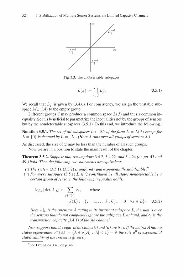
52 3 Stabilization of Multiple Sensor Systems via Limited Capacity Channels
Fig. 3.3. The unobservable subspaces.
L(J) :=⋂
j∈JL−j . (3.5.1)
We recall that L−j is given by (3.4.6). For consistency, we assign the unstable sub-space Munst(A) to the empty group.
Different groups J may produce a common space L(J) and thus a common in-equality. So it is beneficial to parametrize the inequalities not by the groups of sensorsbut by the nondetectable subspaces (3.5.1). To this end, we introduce the following.
Notation 3.5.1. The set of all subspaces L ⊂ Rn of the form L = L(J) except forL = 0 is denoted by L = L. (Here J runs over all groups of sensors J .)
As discussed, the size of L may be less than the number of all such groups.Now we are in a position to state the main result of the chapter.
Theorem 3.5.2. Suppose that Assumptions 3.4.2, 3.4.22, and 3.4.24 (on pp. 43 and49 ) hold. Then the following two statements are equivalent:
(i) The system (3.3.1), (3.3.2) is uniformly and exponentially stabilizable;9
(ii) For every subspace (3.5.1) L ∈ L constituted by all states nondetectable by acertain group of sensors, the following inequality holds:
log2 | detA|L| <∑
j 6∈J(L)
cj , where
J(L) := j = 1, . . . , k : Cjx = 0 ∀x ∈ L . (3.5.2)
Here A|L is the operator A acting in its invariant subspace L, the sum is overthe sensors that do not completely ignore the subspace L at hand, and cj is thetransmission capacity (3.4.1) of the jth channel.
Now suppose that the equivalent claims (i) and (ii) are true. If the matrixA has nostable eigenvalues σ−(A) := λ ∈ σ(A) : |λ| < 1 = ∅, the rate µ0 of exponentialstabilizability of the system is given by
9See Definition 3.4.8 on p. 46.

3.5 Main Result 53
log2 µ0 = max
L∈L
1
dimL
(log2 | detA|L| −
∑
j 6∈J(L)
cj
). (3.5.3)
Moreover, this formula is true whenever σ−(A) 6= ∅ and the quantity in the right-hand side is no less than maxλ∈σ−(A) |λ|.
The proof of this theorem will be given in Sects. 3.7 and 3.8. In Sect. 3.7, weprove its necessity part (i)⇒ (ii). The converse (i)⇐ (ii) is established in Sect. 3.8,where formula (3.5.3) is also justified.
Remark 3.5.3. The quantity log2 | detA|L| from (3.5.2) and (3.5.3) equals the topo-logical entropy10 of the linear system
x(t+ 1) = Ax(t), x(t) ∈ L, x(1) ∈ X1 ⊂ L,
where X1 ⊂ L is an arbitrary compact set for which 0 is an interior (in L) point.
This holds thanks to Theorem 2.4.2 (on p. 21), since the subspaces L ∈ L are A-invariant and all eigenvalues λ of A|L are unstable |λ| ≥ 1 by (3.4.6) and (3.5.1).
By Remark 3.5.3, the quantity log2 | detA|L| represents the unit time incrementof the number of bits required to describe the state of the open-loop (u(·) ≡ 0)system (3.3.1) considered on the invariant subspace L. At the same time, the right-hand side of the inequality from (3.5.2) can be interpreted as the joint capacity of allchannels except for those carrying no information about the state x ∈ L. (The latterchannels serve the sensors that completely ignore such states Cjx = 0 ∀x ∈ L.)Thus the condition (3.5.2) means that the amount of information concerning the statex ∈ L that the decoder may receive over all channels for the unit time exceedsthe unit time growth of the number of bits required to describe the state to a givenhigh accuracy. It should be noted here that some bits counted in (3.5.2) characterizethe state x ∈ L only partly. They correspond to any sensor whose outputs are notsufficient to reconstruct the entire state x ∈ L. Moreover all sensors may be of sucha kind. Nevertheless, when inequalities (3.5.2) are taken for all subspaces L ∈ L,they constitute a sufficient and necessary criterion for stabilizability.
In general, the number of inequalities (3.5.2) does not exceed that of “unstable”invariant subspaces. It also does not exceed the number 2k of all groups J of sensors.Moreover, the inequalities may be directly parameterized by these groups:
log2
∣∣detA|L(J)
∣∣ <∑
j 6∈Jcj . (3.5.4)
Here L(J) is given by (3.5.1) and J ranges over all subsets J ⊂ [1 : k] exceptthose for which L(J) = 0. As discussed, (3.5.4) may contain more inequalitiesthan (3.5.2) does. Indeed, if L(J1) = L(J2) for J1 6= J2, then L(J1) = L(J2) =L(J1∪J2) and so the sets J1, J2, J1∪J2 are served by a single inequality in (3.5.2).At the same time, they give rise to three inequalities in (3.5.4), with those for J = J1
and J = J2 being trivial consequences of the inequality with J = J1 ∪ J2.
10See Definition 2.3.3 on p. 16.

54 3 Stabilization of Multiple Sensor Systems via Limited Capacity Channels
Generally speaking, relations (3.5.2) are not independent. However, revealing“superfluous” inequalities is usually a harder task than direct verification of the entireinequality set (3.5.2).
In general, the conditions for exponential stabilizability at the rate µ are structurallyaltered as µ passes any element ρν of the set
|λ| : λ ∈ σ−(A)
=ρ1 > ρ2 > . . . > ρp
, (3.5.5)
while continuously running over [0, 1). The point is that the “modes” x ∈Mσν fromthe invariant subspace Mσν related to the spectral set
σν :=λ ∈ σ(A) : |λ| = ρν
are stabilized at any rate µ > ρν “for free.” At the same time, their stabilization ata rate µ < ρν requires special efforts and so demands communication resources,which causes alteration of the stabilizability conditions as µ passes ρν .
To extend formula (3.5.3) to the general case, we introduce the following analogsof the subspaces (3.5.1):
Lν(J) := Mσν ∩⋂
j∈JL−oj ,
where the unobservable subspace L−oj of the jth sensor is given by (3.4.6) (on p.49).For consistency, we assign Lν(∅) := Mσν and put L0(J) := L(J).
An exhaustive characterization of the rate of exponential stabilizability is offeredby the following proposition. To simplify notations, its statement proceeds from thestabilizability criterion in the form (3.5.4).
Proposition 3.5.4. Suppose that Assumption 3.4.2 (on p. 43) and (i) of Theorem 3.5.2(on p. 52 ) hold, the pair (A,B) is controllable, and Assumption 3.4.24 (on p. 49) istrue for any elementary spectral set σ ⊂ σ(A). Let ν∗ denote the maximal integerν = 1, . . . , p for which the following set of inequalities holds:
(ν−1∑
α=0
dimLα(J)
)log2 ρν >
ν−1∑
α=0
log2
∣∣detA|Lα(J)
∣∣−∑
j 6∈Jcj
∀J ∈ Ξν :=J ⊂ [1 : k] : L0(J)⊕ L1(J)⊕ · · · ⊕ Lν(J) 6= 0
, (3.5.6)
and ν∗ := 0 if such an integer does not exist.11
The rate µ0 of the exponential stabilizability of the system is given by
log2 µ0 = max
J∈Ξν∗
1∑ν∗α=0 dimLα(J)
ν∗∑
α=0
log2
∣∣detA|Lα(J)
∣∣−∑
j 6∈Jcj
. (3.5.7)
11We suppose that the last case holds whenever σ−(A) = ∅.
Formula (3.5.3) holds only under special circumstances described in Theorem3.5.2.
3.5 Main Result 55
The proof of this proposition will be given in Sect. 3.8.
Remark 3.5.5. It is easy to see that log2
∣∣detA|Lα(J)
∣∣ = dimLα(J) · log2 ρα forα ≥ 1. It follows that, first, whenever (3.5.6) holds for some ν ≥ 1, it also is true forall lesser ν and, second, µ0 ≤ ρν∗ , where ρ0 := 0.
3.5.1 Some Consequences from the Main Result
Remark 3.5.6. The conditions (3.5.2) imply that the system is detectable via the en-tire set of the sensors.
Indeed, otherwise (3.5.2) fails to be true for
L :=
k⋂
j=1
L−j 6= 0
since then the sum in (3.5.2) is over the empty set, which is defined to be 0.
Remark 3.5.7. If the system is detectable by each sensor L−j = 0 ∀j, the set L
contains only one unstable space Munst(A) and so (ii) reduces to only one inequality,
log2 |A|Munst(A)| < c :=
k∑
j=1
cj .
The sum c can be interpreted as the capacity of the channel composed of all channelsat hand. At the same time, log2 |A|Munst(A)| equals the topological entropy H(A)of the open-loop plant (3.3.1) by Theorem 2.4.2 (on p. 21). So the inequality is inharmony with Theorem 2.5.3 (on p. 26) concerning the case of one perfect channel.
3.5.2 Complement to the Sufficient Conditions
The sufficiency part (ii)⇒ (i) of Theorem 3.5.2 can be enhanced by the following.
Proposition 3.5.8. Suppose that Assumptions 3.4.2, 3.4.22, and 3.4.24 (on pp. 43and 49 ) hold and (ii) of Theorem 3.5.2 (on p. 52) is true. Then the system (3.3.1),(3.3.2) is uniformly and exponentially stabilizable by means of simple semirationalr-step recursive coders and a decoder.12
Moreover, coders and decoders of such a kind fit to uniformly and exponentiallystabilize the system at any rate µ exceeding the rate µ0 of exponential stabilizabilityµ > µ0, which is given by (3.5.3).
The proof of this proposition will be given in Sect. 3.8, where a stabilizing controllerwill be described explicitly. It will be shown that the controller exhibits stable behav-ior of its inner dynamical variables zj and z from (3.4.4) and (ii) of Definition 3.4.17(see p. 47).
Remark 3.5.9. The step r can be chosen common for all coders and the decoder.
12See Definitions 3.4.15 and 3.4.17 on p. 47.

56 3 Stabilization of Multiple Sensor Systems via Limited Capacity Channels
3.5.3 Complements to the Necessary Conditions
The (i)⇒ (ii) part of Theorem 3.5.2 can be complemented by the following facts.
Remark 3.5.10. The implication (i) ⇒ (ii) remains true even if Assumption 3.4.24(on p. 49) is dropped.
This easily follows from the proof of this implication presented in Sect. 3.7.If in (3.5.2) the nonstrict inequality sign is substituted in place of the strict one,
the resultant inequalities form necessary conditions for the property that is weakerthan stabilizability. The rigorous statement of this fact is given by the following.
Lemma 3.5.11. Let a controller (3.3.5) exist that makes the trajectories of theclosed-loop system bounded
sup‖x0‖≤K0,t=0,1,...
‖x(t)‖ <∞ ∀K0 > 0. (3.5.8)
Then (ii) of Theorem 3.5.2 holds with < replaced by ≤ in (3.5.2).
Proof. We first show that the property (3.5.8) can be extended on the control:
sup‖x0‖≤K0,t=0,1,...
‖u(t)‖ <∞ ∀K0 > 0. (3.5.9)
To this end, we modify the decoder (3.3.4) by putting U(·) := πU(·), where π is theorthogonal projection from Rnu onto the orthogonal complementMu := (kerB)⊥ tothe kernel kerB := u : Bu = 0. This modification does not alter the action of thecontroller on the plant since B = Bπ. So (3.5.8) is kept true. At the same time, aconstant c > 0 exists such that ‖u‖ ≤ c‖Bu‖ whenever u ∈Mu. So
‖u(t)‖ ≤ c‖Bu(t)‖ (3.3.1)=== c ‖x(t+ 1)−Ax(t)‖ ≤ c ‖x(t+ 1)‖+ c ‖A‖ ‖x(t)‖ .
Thus we see that (3.5.8) entails (3.5.9).Now we pick µ ∈ (0, 1). The transformation
z(t) := µtx(t), v(t) := µtu(t) (3.5.10)
establishes a one-to-one correspondence between the trajectories x(t), u(t) andz(t), v(t) of the open-loop systems given by, respectively, (3.3.1) and the equation
z(t+ 1) = µAz(t) + µBv(t), z(0) = x0. (3.5.11)
We equip the latter with the sensors yj = Cjz, j ∈ [1 : k], the coders
ej(t) = Ej [t, yj(0), µ−1yj(1), µ−2yj(2), . . . , µ−tyj(t)],
and the decoderv(t) = µtU [t, e(t)] .
Here Ej(·) and U(·) are the parts of the controller making the trajectories of theoriginal system bounded. It is easy to see that (3.5.10) still holds for the closed-loop systems. Then Definition 3.4.6 (on p. 46) implies that the proposed coders anddecoder uniformly and exponentially stabilize the system (3.5.11) at the rate µ. Theproof is completed by applying the (i) ⇒ (ii) part of Theorem 3.5.2 to the system(3.5.11) and letting µ→ 1− 0. ⊓⊔

3.6 Application of the Main Result to the Example from Sect. 3.2 57
3.6 Application of the Main Result to the Example from Sect. 3.2
In this section, we justify the statements from Sect. 3.2. We recall that they concerna platoon of k vehicles described by (3.2.1). Each of them is equipped with a sensorgiving the distance yi = xi − xi−1 from it to the preceding vehicle for i ≥ 2 andthe position y1 = x1 for i = 1. It is also served by a communication channel withthe transmission capacity ci > 0 carrying signals to the controller with the sampleperiod ∆ > 0. The objective is to stabilize the platoon motion about a given constant-velocity trajectory: vi = v0
i , xi(t) = x0i + v0
i t ∀i.The substitution of the variables
vi := vi − v0i , xi := xi − x0
i − v0i t
keeps the dynamics equations unchanged and shapes the control goal into xi =0, vi = 0. To put the problem into the discrete-time framework adopted in this chap-ter, we consider the trajectory only at sample times; i.e., we introduce the variables(3.4.9), where now x, v, and u are marked by the lower index i. We also modify thesensor output by subtracting the sensor signal corresponding to the desired trajectory.Then
xi(τ + 1) = xi(τ) + ∆ · vi(τ) +∆2
2ui(τ), vi(τ + 1) = vi(τ) + ∆ · ui(τ),
yi(τ) = xi(τ) − xi−1(τ), (3.6.1)
where x0 := 0. Now
A =
A1 0 0 · · · 00 A2 0 · · · 00 0 A3 · · · 0...
......
......
0 0 0 · · · Ak
, Ai = A = ( 1 ∆
0 1 ) .
The unique elementary spectral set σ = 1 gives rise to k Jordan blocks. Thenonobservable and nondetectable subspaces (3.4.6) coincide and equal
L−j = x := col (z1, w1, . . . , zk, wk) : zj = 0, wj = 0,where zi := xi − xi−1, wi := vi − vi−1,
and x0 := v0 := 0. Assumption 3.4.24 holds with
M iσ := x : zj = 0, wj = 0 ∀j 6= i, i = 1, . . . ,mσ := k.
Assumption 3.4.22 is immediate from (3.6.1). Since | detA|L| = 1 for any invariantsubspace L, Theorem 3.5.2 guarantees that
The platoon is uniformly and exponentially stabilizable under arbitrary transmis-sion capacities ci > 0.

58 3 Stabilization of Multiple Sensor Systems via Limited Capacity Channels
To determine the rate of stabilizability µ0, note that the states nondetectable by(maybe, empty) group J ⊂ [1 : k] of sensors constitute the subspace
L(J) := x : zj = 0, wj = 0 ∀j ∈ J.
Since dimL(J) = 2(k − |J|), where |J| is the size of J, relation (3.5.3) shapes into
log2 µ0 = max
J
1
2(k − |J|)
(−∑
j 6∈J
cj
)= −1
2cmin,
where cmin := minj=1,...,k
cj . (3.6.2)
It follows that
For the platoon at hand, the rate of the exponential stabilizability equals√
2−cmin
per sample period.
Now consider the situation where the sensor system accommodated by each ve-hicle gives the distances to l < k vehicles to the right, as well as to l vehicles to theleft. (We assume an imaginary vehicle that is numbered by 0 and stays at the origin.)Then clearly
L−j =x : zi = 0, wi = 0 ∀i = maxj − l + 1, 1, . . . ,minj + l, k
.
Assumption 3.4.24 remains true with the same subspaces M iσ , and the platoon evi-
dently remains uniformly and exponentially stabilizable. What can be said about therate of stabilizability? Now the collection L introduced in Notation 3.5.1 (on p. 52)consists of spaces L(J) related to sets J, which along with any element j ∈ J containa certain interval of the form
[i− l + 1 : i+ l] ∩ [1 : k] ∋ j, i = 1, . . . , k.
Such sets are said to be wide. To proceed, we consider separately two cases.1. Let 2l ≥ k. Then any two aforementioned intervals contain a common point.
It follows that apart from J = ∅, the wide sets J are only intervals of the form
[1 : i], i ≥ l + 1, or [i : k], i ≤ k − l + 1.
By retracing (3.6.2), we see that µ0 =√
2−ck,l , where ck,l is given by (3.2.2) (on
p. 41).2. Now let 2l < k. Then the sets
[1 : i− 1] ∪ [i+ 1 : k], i = l + 2, . . . , k − l,[i : k], i = 2, . . . , l+ 2,
[1 : i], i = k − l, . . . , k − 1
3.7 Necessary Conditions for Stabilizability 59
are wide. By restricting the maximum in (3.6.2) to only these sets J, we see that
µ0 ≥√
2−ck,l , where ck,l is given by (3.2.2) (on p. 41). In fact, µ0 =
√2−ck,l . To
prove this, it suffices to show that
1
k − |J|∑
j 6∈J
cj ≥ ck,l (3.6.3)
for any wide set J. To this end, we put
i− := minj : j ∈ J and i+ := maxj : j ∈ J.
Then
i− ≤ l + 1⇒ [i− : l + 1] ⊂ J and i+ ≥ k − l + 1⇒ [k − l + 1 : i+] ⊂ J
by the definition of the wide set. Hence
j : j 6∈ J = J1 ∪ · · · ∪ Js,
where the sets Jν are pairwise disjoint and each of them has the form
Jν = i, i = l + 2, . . . , k − l, or
Jν = [1 : i], i = 1, . . . , l + 1, or
Jν = [i : k], i = k − l + 1, . . . , k.
By (3.2.2) (on p. 41),1
|Jν |∑
j∈Jν
cj ≥ ck,l.
This implies (3.6.3) as follows:
1
k − |J|∑
j 6∈J
cj =1
k − |J|
s∑
ν=1
|Jν |1
|Jν |∑
j∈Jν
cj ≥ ck,l.
3.7 Necessary Conditions for Stabilizability
3.7.1 An Extension of the Claim (i) from Theorem 2.5.3 (on p. 26)
This theorem deals with an instantaneous and lossless channel. Now we show that itsstatement (i) remains true for delayed and lossy channels considered in this chapter.For technical reasons, which will become clear soon, we extend the class of systemsand consider ones of the following form
x(t + 1) = Ax(t) + B[t, u(0), . . . , u(t)], (3.7.1)
where B(·) is a given function. We also recall that the matrix A is unstable.

60 3 Stabilization of Multiple Sensor Systems via Limited Capacity Channels
Lemma 3.7.1. Suppose that there is only one channel k = 1. Then H(A) < c := c1whenever the system (3.7.1) is uniformly and exponentially stabilizable. Here H(A)is the topological entropy (2.4.2) (see p. 21) of the open-loop system (3.3.1).
Proof. Suppose first that H(A) > c. By putting
v(t) := B[t, u(0), . . . , u(t)], X1 := x : ‖x‖ ≤ 1, and B := I,
we shape (3.7.1) into (2.5.1) (on p. 24) with u(t) := v(t). From this point, the proofproceeds by merely retracing the arguments from the proof of (i) from Theorem 2.5.3(see p. 30), where T := 1 and R ∈ (c, H(A)) are taken. However when the set Sof all possible control sequences v(0), . . . , v(T ) is examined, it should be noted thatnow its size |S| does not exceed 2b
+1 (T ) by (i) of Assumption 3.4.2 (on p. 43). At the
same time, limT→∞ b+1 (T )/T = c < R due to (3.4.1) (on p. 43). So log2 |bS|T < R if
T is large enough, which keeps all arguments from the proof of (i) of Theorem 2.5.3true and so entails a contradiction to the stabilizability of the system.
Thus H(A) ≤ c. To prove the strict inequality H(A) < c, we employ the hintsimilar to that from the proof of Lemma 3.5.11 (on p. 56). In other words, we con-sider the process x∗(t) := κtx(t). It clearly satisfies the equation of the form (3.7.1)
x∗(t+ 1) = κAx∗(t) + κt+1B[t, u(0), . . . , u(t)].
To keep this system stable, the constant κ > 1 is chosen so that κµ < 1, where µ istaken from (3.4.2) (on p. 46). Then by the foregoing,H(κA) ≤ c. It remains to notethat H(κA) > H(A) owing to (2.4.2) (on p. 21). ⊓⊔
Lemma 3.7.1 evidently remains true if the regime of the channel operation (givenby τ1(·)) is known in advance.
3.7.2 An Auxiliary Subsystem
To prove (3.5.2) (on p. 52), we revert to the system (3.3.1) and pick a subspaceL ∈ L
constituted by the states not detectable by a certain group of sensors. Then we restrictourselves to trajectories x(t)∞t=0 starting at x0 ∈ L and apply Lemma 3.7.1 tothem. More precisely, we take into account that x(t) may leave L due to controls,and we consider xL(t) := πx(t). Here π is a projector from Rn onto L. It is easy tocheck that the evolution of xL is governed by the equation of the form (3.7.1):
xL(t+ 1) = A|LxL(t) + πBu(t) +t−1∑
i=0
(πA−Aπ)At−1−iBu(i),
xL(t) ∈ L, xL(0) = x0. (3.7.2)
Remark 3.7.2. The first equation simplifies if πA = Aπ. However, such a projectorπ exists if and only if an A-invariant subspace exists that is complementary to L,which is not true in general.

3.7 Necessary Conditions for Stabilizability 61
Notation 3.7.3. For I ⊂ [1 : k], the symbol CI denotes the block matrix that resultsfrom arranging the blocks Ci with i ∈ I into a column.
For any entities vi enumerated by i ∈ [1 : k], the symbol vI is defined likewise.
We interpret (3.7.2) as equations of an imaginary system and equip it with the sensor
yL(t) = CJcxL(t). (3.7.3)
Here Jc := j : j 6∈ J is the complement to the set
J = j : Cjx = 0 ∀x ∈ L
of sensors ignoring the subspace L. We also suppose that all channels with j 6∈ J arecommissioned to transmit yL.
The sum in the right-hand side of (3.5.2) (on p. 52) equals the capacity of theunion of these channels. Hence (3.5.2) follows from Lemma 3.7.1 applied to thesystem (3.7.2), (3.7.3). To complete the proof, it suffices to show that this systemis stabilizable whenever the original one (3.3.1), (3.3.2) can be stabilized. In doingso, one must cope with the fact that the trajectory of the original closed-loop system(3.3.1)–(3.3.4) may leave the subspace L. So the observations (3.3.2) and the entriesof (3.7.3) may differ. Moreover, the sensors omitted in (3.7.3) may see the state x(t)for t ≥ 1. It should be shown that they are yet useless and can be dropped.
3.7.3 Stabilizability of the Auxiliary Subsystem
Lemma 3.7.4. Let the system (3.3.1), (3.3.2) be exponentially stabilized by somecontroller, and let the regime of the channels operation be known in advance. Thenthe system (3.7.2), (3.7.3) is also exponentially stabilizable.
Proof. We first show that for x0 ∈ L, the process in the original closed-loop systemobeys the relations
eJ(t) = E′j[t, eJc(t− 1)
],
yJ(t) = Y′[t, eJc(t− 1)
], yJc(t) = yL(t) + Y′′
[t, eJc(t− 1)
]. (3.7.4)
We recall that the data ej(t) that arrived via the jth channel by time t is given by(3.3.6) (on p. 42). The observation yL(t) is defined by (3.7.2) and (3.7.3) for thesequence of controls u(t) identical to that driving the original system.
For t = 0, we have
x(0) ∈ L⇒ yJ(0) = 0 and yJc(0) = yL(0).
So (3.7.4) with t = 0 follows from (3.3.3). Now suppose that (3.7.4) with t := θholds for all θ ≤ t. Then
eJ (θ) = E′[θ, eJc(t− 1)
]

62 3 Stabilization of Multiple Sensor Systems via Limited Capacity Channels
and so
e(θ) = [eJ (θ), eJc(θ)] = E[θ, eJc(t)
] (3.3.4)==⇒ u(θ) = U′
[θ, eJc(t)
](3.7.5)
for θ ≤ t. Now we invoke (3.3.1) and note that
x0 ∈ L⇒ At+1x0 ∈ L⇒ CJAt+1x0 = 0 and (I − π)At+1x0 = 0.
As a result, we see that
yJ(t+ 1) = CJAt+1x0︸ ︷︷ ︸
=0
+
t∑
θ=0
CJAt−θBu(θ) =: Y′
[t+ 1, eJc(t)
],
yJc(t+ 1)− yL(t+ 1) = CJc
[x(t+ 1)− πx(t + 1)
]= CJc(I − π)At+1x0︸ ︷︷ ︸
=0
+ CJc
t∑
θ=0
(I − π)At−θBu(θ) =: Y′′[t+ 1, eJc(t)
];
i.e., the last two relations from (3.7.4) do hold with t := t+ 1. Then the first relationfollows from (3.3.3).
It follows from (3.3.3) and (3.7.4) that the signal eJc(t) is determined by theprior measurements from (3.7.3),
eJc(t) = EL[t, yL(0), . . . , yL(t)].
Now we interpret this as the equation of the coder and the last relation from (3.7.5)(where θ := t) as that of the decoder for the system (3.7.2), (3.7.3). By the forego-ing, this coder–decoder pair generates the trajectory πx(t), u(t), t = 0, 1, . . ., wherex(t), u(t) is the trajectory of the original closed-loop system. So the inequalities(3.4.2) (on p. 46) are inherited by the system (3.7.2), (3.7.3), which completes theproof. ⊓⊔
3.7.4 Proof of the Necessity Part (i) ⇒ (ii) of Theorem 3.5.2
As discussed, this implication is immediate from Lemmas 3.7.1 and 3.7.4.
3.8 Sufficient Conditions for Stabilizability
In this section, we suppose that the assumptions and (ii) of Theorem 3.5.2 (on p. 52)hold, and until stated otherwise, adopt one more assumption.
Assumption 3.8.1. The system (3.3.1) has no stable |λ| < 1 eigenvalues λ.
In the general case, a stabilizing controller will be obtained by applying that pre-sented below to the unstable part of the system.

3.8 Sufficient Conditions for Stabilizability 63
3.8.1 Some Ideas Underlying the Design of the Stabilizing Controller
To stabilize the system, we employ the scaled quantization scheme (see, e.g., [28,73,135,136,149,184,204]). It was mainly developed for only one channel and is brieflyas follows. Both coder and decoder compute a common upper bound δ of the currentstate norm ‖x‖∞ := maxi |xi|. They are also given a partition of the unit ball intomballs (cubes) with small radii ≤ ς(m). The number m matches the channel capacityso that the serial number of the cube can be communicated to the decoder. The coderdetermines the current state from the observations and notifies the decoder whichcube contains this state divided by δ. Since the decoder knows δ, it thus becomesaware of a ball B with the radius ≤ δς(m) containing the current state. Then itselects a control that drives the system from the center of this ball to zero. The ballitself is expanded because of the unstable dynamics of the system and transformedinto a set D+(B) centered about zero: D+(B) ⊂ Bα0 . So the radius α can be takenas a new upper bound δ. Here α ≤ δς(m)µ, where µ characterizes the expansionrate of the system. If ς(m)µ < 1, the bound δ is thus improved δ := δς(m)µ < δand by continuing likewise, it is driven to zero δ → 0, along with the state x.
In the context of this paper, a problem with the above scheme is that no coder maybe aware of the entire state x. So a natural idea [204] is to disintegrate the system(3.3.1) into subsystems each observable by some sensor. Then each subsystem can bestabilized by following the above lines, provided the stability condition ς(m)µ < 1holds for it. In fact, this condition means that there is a way to communicate a suffi-ciently large amount of information from the subsystem to the decoder: the smallerthe radius ς(m), the larger the size m of the partition, and so the larger the numberof bits required to describe which of m cubes contains the state.
No channel in itself may meet the above stability condition. At the same time,this condition may be met if several channels are commissioned to transmit infor-mation about a given subsystem. Then each channel may carry only a part of thisinformation, whereas the decoder assembles these parts, thus getting the entire mes-sage (see Fig. 3.4). Certainly, these channels should be chosen among those servingthe sensors that observe the subsystem at hand.
Fig. 3.4. Distribution of data over parallel channels.

64 3 Stabilization of Multiple Sensor Systems via Limited Capacity Channels
Since a given sensor may observe several subsystems, the above scheme meansthat each channel must transmit a set of messages each concerning a particular sub-system (see Fig. 3.5a). As a result, each subsystem is served by a variety of channels,whereas every channel is fed by several subsystems (see Fig. 3.5b). This gives rise to
Subsystems Channels
Fig. 3.5(a). Data transfer over a givenchannel.
Fig. 3.5(b). Data transfer over all chan-nels.
the question: Is it possible to distribute the required information about each particularsubsystem over parallel channels in such a way that the total amount of informationcarried via every channel meets its capacity? It will be shown via convex dualityarguments that the answer is in the affirmative whenever (ii) of Theorem 3.5.2 holds.
Another problem is how to employ a sensor observing the subsystem only partly.Certainly, this problem does not hold if there are no such sensors and subsystems:The state of each subsystem either is completely determined from or does not af-fect the outputs of any given sensor. Decomposition into a set of such subsystemsis possible. However, in general, these subsystems are dependent. The reasons forthis are twofold. First, the control is common. Second, Jordan blocks may entail anunavoidable interinfluence between the states of the subsystems.
To illustrate the last claim, we invoke the system (3.4.11) (on p. 51) whose dy-namical matrix is the standard Jordan block. The unobservable subspaces of the sen-sors are given by (3.4.12). There are no other invariant proper subspaces.13 So thissystem cannot be decomposed into subsystems with independent open-loop dynam-ics. At the same time, any sensor except for the last one observes the state x onlypartly. So to exclude such a partial vision, disintegration into state-dependent sub-systems is unavoidable.
To deal with them, we employ sequential stabilization. We define the sth subsys-tem as that described in the sth row from (3.4.11). Its state is xs. Then we stabilizethe first subsystem, which is independent of the others. This makes x1 exponentiallydecaying. In the equations of the second subsystem, we interpret x1 as an exogenousdisturbance. By constructing a device stabilizing this subsystem under any exponen-tially vanishing disturbances, we make x2 exponentially decaying. The entire systemis stabilized by continuing likewise.
These arguments, however, do not take into account that the control affects allsubsystems, and some of them may be unstabilizable (although the entire system
13See the proof of Lemma 3.8.3 on p. 66.

3.8 Sufficient Conditions for Stabilizability 65
is controllable). For example, the subsystems with s ≥ 2 are unstabilizable if b1 =1, b2 = · · · = bd = 0 in (3.4.11). This obstacle can be easily overcome via increasingthe sample period.
Indeed, let us pick r = 1, 2, . . .. The state xi := x(ir) evolves as follows:
xi+1 = Arxi + BU i, (3.8.1)
where
U i := col[u(ir), u(ir + 1), . . . , u(ir + r − 1)
]and
BU :=
r−1∑
j=0
Ar−1−jBuj (3.8.2)
is the state to which the control program U = col[u0, . . . , ur−1
]drives the system
at time t = r from x(0) = 0. Since the system (3.3.1) with no stable modes iscontrollable by Assumption 3.4.22 (on p. 49), the operator B is onto if r ≥ n.Related to the decomposition of the system state x = col (x1, . . . , xd) into the statesxi of subsystems is a block partition
BU = col[B1U , . . . ,BdU
].
Since all operators Bs have full rank, any subsystem is controllable. Moreover, anycontrol action y = BsU in the sth subsystem can be implemented by a control U
that does not disturb the other subsystems: BjU = 0 ∀j 6= s.
3.8.2 Plan of Proving the Sufficiency Part of Theorem 3.5.2
Summarizing, we adopt the following plan.
Step 1. We decompose the system so that, first, for any given sensor, the state of eachsubsystem either does not affect or is determined from the sensor outputsand, second, the decomposition is triangular. The latter permits us to employthe sequential stabilization approach.
Step 2. We increase the sample period and, for each subsystem, offer a class of con-trollers stabilizing it under any exponentially decaying disturbance. In doingso, we assume that the coder is aware of the current state at any sample timet = ir, and there is a way to communicate as much information as desiredfrom the coder to the decoder.
Step 3. Within the above class, we point out the controller that requires a nearlyminimum bit-rate of such a communication.
Step 4. We show that if all subsystems are equipped with these controllers, the entiresystem is stabilized.
Step 5. We obtain conditions under which the entire set of these controllers can beimplemented14 by means of real channels and sensors. These conditions arenot constructive and require that a linear system of inequalities be solvablein integers.
14In particular, the required information traffic can be arranged.

66 3 Stabilization of Multiple Sensor Systems via Limited Capacity Channels
Step 6. By employing convex duality arguments, we show that these conditions areequivalent to (ii) of Theorem 3.5.2.
Step 7. We drop Assumption 3.8.1 and show that (ii) of Theorem 3.5.2 suffices tostabilize the system with both unstable and stable eigenvalues (modes).
3.8.3 Decomposition of the System
Now we perform step 1 of the above plan. In other words, we represent the systemas a set of subsystems interacting in a special manner. The main result is as follows.
Proposition 3.8.2. Suppose that Assumption 3.8.1 (on p. 62) holds. Then after aproper one-to-one linear transformation and partition of the state
x = col (x1, . . . , xd) (3.8.3)
into several blocks xs ∈ Rns interpreted as the states of subsystems, the followingstatements hold:
(i) The unobservable subspace (3.4.6) (see p. 49) L−oj = L−j of any sensor iscomposed of several blocks:
L−j = x : xs = 0 ∀s ∈ Oj , where Oj ⊂ [1 : d];
(ii) The block representation of the dynamics equations (3.3.1) is lower triangular:
xs(t+ 1) =s∑
i=1
Asixi(t) +Bsu(t), s = 1, . . . , d. (3.8.4)
By (i), the states xs of subsystems s 6∈ Oj do not affect the outputs of the jthsensor, whereas the states xs with s ∈ Oj are uniquely determined from these out-puts.
The remainder of the subsection is devoted to the proof of Proposition 3.8.2. Westart with two technical facts.
Lemma 3.8.3. The claim (i) of Assumption 3.4.24 (on p. 49) holds for any elemen-tary spectral set σ.
Proof. In view of Assumption 3.4.24, it suffices to prove the lemma assuming thatthe set σ gives rise to only one real Jordan block. We putM := Mσ, Aσ := A|M andnote that det[λI−Aσ] = ϕ(λ)p, where the polynomialϕ is irreducible over the fieldof real numbers. By employing the basis in M reducing Aσ to the real Jordan form,it is easy to see that the formula L(ν) := ker
[ϕ(Aσ)
]νproduces (p+ 1) distinct
0 = L(0) ⊂ L(1) ⊂ · · · ⊂ L(p) = M
invariant subspaces and dimL(ν) = ν degϕ. We are going to show that there are noother invariant subspaces.

3.8 Sufficient Conditions for Stabilizability 67
Indeed let L be such a subspace and ψ be the minimal annihilating polynomialof L. Then ψ is a divisor of ϕp and so ψ = ϕν , ν = 0, . . . , p. Hence
L ⊂ ker[ϕ(Aσ)
]ν= L(ν).
At the same time, Theorem 2 of [61, p. 180] implies that dimL = degψ. ThusdimL = ν degϕ = dimL(ν), and so L = L(ν).
As a result, we see that all invariant subspaces L−j ∩Mσ are among L(0), . . .,L(p). It remains to pick M1
σ := L(1),mσ := p, and for i = 2, . . . , p, choose M iσ so
that L(i− 1)⊕M iσ = L(i). ⊓⊔
The next lemma plays the key role in the proof of Proposition 3.8.2.
Lemma 3.8.4. In Assumption 3.4.24 (on p. 49), the atoms M iσ, i = 1, . . . ,mσ , can
be chosen so that all partial direct sums of the form
M1σ ⊕ · · · ⊕M i
σ, i = 1, . . . ,mσ,
are A-invariant.
Proof. We consider the set of atoms with the minimal sizemσ. We also introduce theundetectable subspaces Lj := L−j ∩Mσ of Mσ, then we form all their intersections
L∩ = Lj1 ∩ · · · ∩ Ljp ,
and then we form all algebraic sums (not necessarily direct) of such intersections
LΣ = L∩i1 + · · ·+ L∩ir .
Here p, r and the subspaces Ljν , L∩iµ are chosen arbitrarily. Let M denote the set ofall LΣ’s. It is clear that
1) Any space L ∈ M is invariant and decomposable into a direct sum of severalatoms;
2) L ∈M⇒ L ∩ Lj ∈M ∀j;3) Mσ ∈M;4) L′, L′′ ∈M⇒ L′ + L′′ ∈M;5) The set M is finite.
Now we pick a minimal element Lmin among L ∈M, L 6= 0, i.e., such that
L ⊂ Lmin & L ∈M & L 6= 0 ⇒ L = Lmin.
By trying here L := Lmin ∩ Lj , we see that either Lmin ⊂ Lj or Lmin ∩ Lj = 0.Hence any Lj contains either all atoms constituting Lmin or none of them. So theseatoms can be replaced by their sum in (i) of Assumption 3.4.24. Since the numberof all atoms is minimal, only one atom is concerned:Lmin = Mν
σ . By permuting theatoms, we set ν = 1. Then the claim of the lemma does hold for i = 1 by 1).

68 3 Stabilization of Multiple Sensor Systems via Limited Capacity Channels
Now let Lmin denote a minimal element among L ∈ M such that L ⊃ M1σ and
L 6= M1σ . By 2) and 4),
L := M1σ + Lj ∩ Lmin ∈M.
So the minimum property yields that either L = M1σ or Lmin ⊂ L. In terms of the
decomposition from 1)Lmin = M1
σ ⊕Mmin ∈M
(where Mmin is the sum of several atoms), this means that either Mmin ∩ Lj = 0or Mmin ⊂ Lj . Like above, this implies that Mmin consists of only one atom Mν
σ .By permuting the atoms, we set ν = 2, thus making the claim of the lemma true fori = 2 by 1). The proof is completed by continuing likewise. ⊓⊔
Proof of Proposition 3.8.2. We decompose the spectrum
σ(A) = σ1 ∪ · · · ∪ σp
into the union of disjoint elementary sets. Then
Rn = Mσ1 ⊕ · · · ⊕Mσp ,
and any invariant subspace L−j is decomposed
L−j = L−j (1)⊕ · · · ⊕ L−j (p)
into the invariant subspaces L−j (ν) := L−j ∩Mσν . So it suffices to show that, for anyν, linear coordinates in Mσν and their block partition exist for which any subspaceL−j (ν), j = 1, . . . , k, is the direct sum of several “blocks” and the operator A|Mσν
has a lower triangular form with respect to this partition. These blocks zi are in factgiven by Lemma 3.8.4:
zi ∈Mmσν−i+1σν .
More precisely, it suffices to pick a basis in each subspace M iσν , i = 1, . . . ,mσν ,
unite them to produce a basis in Mσν , and then consider the coordinates with respectto this basis and their partition that corresponds to the partition z = z1 + · · ·+ zmσν
of z into zi ∈Mmσν−i+1σν . ⊓⊔
3.8.4 Separate Stabilization of Subsystems
In this subsection, we perform step 2 (see p. 65) of the plan from Subsect. 3.8.2.
Introducing Subsystems
We pick an integer parameter r and focus attention only on the states at times τi =i · r. The evolution of these states is given by (3.8.1) (on p. 65), which evidentlyinherits the lower triangular structure from (3.8.4),
3.8 Sufficient Conditions for Stabilizability 69
xsi+1 =s∑
ν=1
A(r)sν x
νi + BsUi (3.8.5)
for s = 1, . . . , d. Here
xsi := xs(τi), Ui = col[u(τi), . . . , u(τi + r − 1)
],
and the diagonal coefficients from (3.8.5) are the rth powers of the matching coeffi-cients from (3.8.4), A(r)
ss = Arss.The sth subsystem is described by the following equations:
xsi+1 = Arssxsi + BsUi + ξs,i, i = 0, 1, . . . . (3.8.6)
Here in accordance with (3.8.5),
ξs,i(t) ≡ 0 for s = 1 and ξs,i(t) =
s−1∑
ν=1
A(r)sν x
νi otherwise. (3.8.7)
In this subsection, we ignore this rule and interpret ξs,i(t) as an exogenous dis-turbance. This permits us to study each subsystem independently of the others. Wealso suppose that the disturbance decays at a known rate ρξ:
|ξs,i| ≤ Kξρiξ, ρξ ∈ [0, 1), i = 0, 1, . . . (3.8.8)
with Kξ unknown, and offer a controller that stabilizes the sth subsystem under allsuch disturbances. In doing so, we assume that the current state xsi is measured on-line. The proposed controller uses only finitely many bits of information about xsi .
Remark 3.8.5. The controller will be mainly based on the ideas from [28, 73, 77,135, 136, 149, 184, 201, 204]. Major distinctions concern two points. First, we takeinto account exogenous disturbances decaying at a known rate. Second, we considerthe case where the transmission of the above bits to the decoder takes some time(specifically, r units of time). This implies complements to the stabilization scheme,e.g., the need to quantize not the current state but the state prognosis.
We first introduce components of which the coder and the decoder will be assembled.
Quantizer
To communicate a continuous sensor data over a discrete (digital) channel, an analog-to-digital converter is required.
Definition 3.8.6. An m-level quantizer Qs in Rns is a partition of the closed unitballB1
0 ⊂ Rns with respect to some norm ‖ ·‖ intom disjoint setsQ1, . . . , Qm eachequipped with a centroid qQi ∈ Qi.Such a quantizer converts any vector xs ∈ Qi into its quantized value Qs(xs) := qQi
and any vector xs 6∈ B10 outside the unit ball into an alarm symbol Qs(xs) := z.

70 3 Stabilization of Multiple Sensor Systems via Limited Capacity Channels
Definition 3.8.7. The quantizer is said to be r-contracted (for the sth subsystem) if
Arss(Q− qQ
)⊂ ρQsB1
0 ∀Q = Qi, i = 1, . . . ,m, where ρQs ∈ (0, 1). (3.8.9)
The constant ρQs ∈ (0, 1) is called the contraction rate.
Definition 3.8.8. The quantizer is said to be polyhedral if the quantizer map Qs(·)is semialgebraic15 with linear functions li(xs) = a T
i xs + bi, i ∈ [1 : M s] in (3.4.3)
(on p. 46).
In other words, such a quantizer acts by checking the linear inequalities li(xs) ≥0, i ∈ [1 : Ms] and forming the tuple A(xs) whose ith entry is 1 (yes) if the inequal-ity is satisfied and 0 (no) otherwise. The quantizer output is uniquely determined bythe distribution of answers (yes, no) over the set of inequalities, i.e., by this tuple.
Remark 3.8.9. Not only nonstrict but also strict inequalities can be considered here.This holds since the results of checking the strict li(xs) > 0 and nonstrict−li(xs) ≥0 inequalities, respectively, are uniquely determined from each other by the negation.
Remark 3.8.10. For polyhedral quantizers, any level domain Qi (along with Qz :=xs : Qs(xs) = z) is the union of a finite number of convex polyhedra.
Note also that for such quantizers, the ball from Definition 3.8.6 is a convex polytop.
Example 3.8.11. One of the simplest examples of a quantizer is given by the uniformpartition of the square with the side length 2 into m = N2 congruent subsquares(see Fig. 3.6, where N = 12). The norm in Definition 3.8.6 is given by ‖x‖∞ =max|x1|, |x2|, x = col (x1, x2). The centroid is the center of the correspondingsubsquare. This quantizer is polyhedral and served by 2(N + 1) linear inequalities:
x1 ≥ −1 + (i− 1)2
N, i = 1, . . . , N, x1 > 1,
x2 ≥ −1 + (i− 1)2
N, i = 1, . . . , N, x2 > 1. (3.8.10)
In this case, it is convenient to split the tuple A(x) of answers into two subtuplesA1(x) and A2(x) related to the first and second subsets of inequalities, respectively.If all entries of either A1(x) or A2(x) equal each other (all are 1 or all are 0), thequantizer output is z. Otherwise
Qs(x) = col(−1 + [i1 − 1]
2
N+
1
N,−1 + [i2 − 1]
2
N+
1
N
),
where iν (for ν = 1, 2) is the maximal serial number of the inequality for which theaffirmative answer 1 is written in the tuple Aν(x).
15See Definition 3.4.9 on p. 46.

3.8 Sufficient Conditions for Stabilizability 71
Fig. 3.6. Uniform square quantizer.
Explanation 3.8.12. In (3.8.10), the strict inequalities are taken for i = N to makethe quantizer’s effective domain x : Qs(x) 6= z closed, as is required by Defini-tion 3.8.6.
Remark 3.8.13. Example 3.8.11 is easily generalized on the case of the general Eu-clidean space Rns . Then the uniform partition of the cube with side length 2 intoNns congruent subcubes is performed. The centroid is the center of the correspond-ing subcube. This quantizer is still polyhedral.
Remark 3.8.14. The last example entails that for any r, a polyhedral r-contractedquantizer exists.
Indeed, the set Q − qQ, Q = Qi from (3.8.9) is the cube with side length 2/Ncentered about zero. Equivalently, this is the ball of radius 1/N with respect to thenorm
‖xs‖∞ := max|xs1|, . . . , |xsns
|, xs = col
(xs1, . . . , x
sns
). (3.8.11)
So to ensure (3.8.9), it suffices to pick N > ‖Arss‖∞, where ‖ · ‖∞ is the matrixnorm matching (3.8.11): ‖A‖∞ := max‖xs‖∞=1 ‖Axs‖∞.
Assumption 3.8.15. In the remainder of this subsection, we suppose that a polyhe-dral r-contracted quantizer is given (for any r).
As will be shown, the number of its levels determines the communication bit raterequired for stabilization. So an r-contracted quantizer with the minimal number oflevels is of special interest. Such a quantizer will be offered in Subsect. 3.8.5.
Deadbeat Stabilizer
This is a linear transformation N of an initial state xs0 into a control program U thatdrives the unperturbed ξs,i ≡ 0 subsystem (3.8.6) to zero,

72 3 Stabilization of Multiple Sensor Systems via Limited Capacity Channels
0 = xs1(= xs(r)) = Arssxs0 + BsU for U := Nxs0 and any xs0. (3.8.12)
A particular deadbeat stabilizer with advanced properties16 will be proposed in Sub-sect. 3.8.6.
Assumption 3.8.16. In the remainder of this subsection, we suppose that a deadbeatstabilizer is given.
Parameters
Apart from r, the controller employs two more parameters ρ and γ chosen so that
r > n, γ > ‖Ass‖r, and 1 > ρ > maxρξ, ρQs, (3.8.13)
where Ass, ρξ, and ρQs are taken from (3.8.4), (3.8.8), and (3.8.9), respectively.
Description of the Coder and Decoder
Both coder and decoder compute controls U ci , U d
i and upper bounds δci , δdi for the
state norm ‖xsi ‖, respectively. Actually, acting upon the plant is the control U di . The
initial bounds are common: δc0 = δd0 = δ0 > 0. (The inequality δ0 ≥ ‖xs0‖ may beviolated.) At any time τi = ir, the coder selects a finite-bit message based on xsi andsends it to the decoder. We suppose that this message arrives by time τi+1.
Specifically, the coder and decoder operate as follows.
The sth coder (at the times t = τi, i = 1, 2, . . .)
c.1) Proceeding from the knowledge of the current state xsi , computes the prognosisxsi+1 of the state at t = τi+1,
xsi+1 := Arssxsi + BsU
ci ; (3.8.14)
c.2) Employs the r-contracted quantizer Qs to compute the quantized value qi ofthe scaled state at t = τi+1,
εi :=[δci]−1
xsi+1, qi := Qs[εi]; (3.8.15)
c.3) Encodes this quantized value qi for transmission and sends it to the decoder;c.4) Computes the next control program by means of the deadbeat stabilizer N and
corrects the upper bound,
U ci+1 := N
[δci
⋆qi], δci+1 := δci × 〈qi〉ρ,γ , where (3.8.16)
⋆q:=
q if q 6= z,
0 otherwise,〈q〉ρ,γ :=
ρ if q 6= z,γ otherwise,
. (3.8.17)
16These properties are beneficial when all subsystems are stabilized simultaneously.

3.8 Sufficient Conditions for Stabilizability 73
The sth decoder (at the times t = τi, i = 2, 3, . . .)
d.1) Decodes the newly received data and thus acquires qi−1;d.2) Computes the current control program and corrects the upper bound,
U di := N
[δdi
⋆qi−1
], δdi+1 := δdi × 〈qi−1〉ρ,γ . (3.8.18)
Remark 3.8.17. For definiteness, the initial control programs U c0 ,U
d0 ,U
c1 ,U
d1 are
taken to be zero.
Explanation 3.8.18. We introduced separate controls U ci ,U
di and bounds δci , δ
di to
stress that the coder and decoder compute them independently. However, it easilyfollows from (3.8.16), (3.8.18) and induction on i that they in fact coincide,
δdi = δci−1, Udi = U
ci , i = 1, 2, . . . . (3.8.19)
Remark 3.8.19. The second relation from (3.8.19) implies that the error in the stateprognosis (3.8.14) is equal to the disturbance from (3.8.6),
xsi+1 = xsi+1 − ξs,i. (3.8.20)
Explanation 3.8.20. To be communicated across the channel, the quantized value qishould be encoded into a code word
(es[ir], es[ir + 1], . . . , es[(i+ 1)r − 1]
)∈ Ers,
whose symbols are consecutively emitted into the sth channel during the forthcomingoperation epoch [ir : (i+ 1)r).
Remark 3.8.21. Letm denote the number of the quantizer levels.17 By c.3), the codersends on average log2(m+1)
r bits per unit time to the decoder.
In Subsect. 3.8.5, the minimum of this ratio over r-contracted quantizers will bestudied.
Observation 3.8.22. As follows from Definitions 3.4.15 and 3.4.17 (on p. 47), theproposed coder and decoder are simple semirational one-step recursive.
We recall that the sample period was increased so that now one step is equivalent tor former ones.
Remark 3.8.23. The inner dynamical variables zs(= zs) and z of the coder and de-coder (see Definitions 3.4.15 and 3.4.17) can be defined as zsi := (δci ,U
ci ), zi := δdi .
Stabilizing Properties of the Coder and Decoder
These properties are revealed by the following main result of the subsection.
Proposition 3.8.24. Suppose that Assumption 3.8.1 (on p. 62) and (3.8.13) hold, andthe disturbance in the sth subsystem (3.8.6) satisfies (3.8.8). Then the above coder–decoder pair uniformly and exponentially stabilizes this subsystem:
‖xsi‖ ≤ Kxρi, ‖U d
i ‖ ≤ Kuρi ∀i ≥ 0 whenever ‖xs0‖ ≤ K0. (3.8.21)
Here ρ < 1 is the parameter of the controller from (3.8.13), and the constantsKx,Ku may depend on Kξ from (3.8.8) and K0.
17Hence with regard to the extra alarm symbol, the quatizer output can take m + 1 values.

74 3 Stabilization of Multiple Sensor Systems via Limited Capacity Channels
Proof of Proposition 3.8.24
The remainder of the subsection is devoted to this proof, which is broken into thestring of several lemmas. We start with rough estimates of concerned variables.
Lemma 3.8.25. The following inequalities hold for all i ≥ 1, h ≥ 0, and p ≥ h:
δ0ρi−1 ≤ δci ≤ δ0γi−1, ‖U d
i ‖ ≤ ‖N‖δci−1,
‖xsp‖ ≤ ar(p−h)s
[‖xsh‖+K ′ξρ
hξ
]+Kγγ
p|I(p, h)|, (3.8.22)
where K ′ξ := Kξ/(ars − 1) and as is an arbitrary constant such that
as > ‖Ass‖, (3.8.23)
|I(p, h)| is the size of the set
I(p, h) := j = h, . . . , p− 1 : j ≥ 2 & qj−1 6= z,
and the constant Kγ does not depend on x0,K0, h, p,Kξ.
Remark 3.8.26. Due to Assumption 3.8.1 (on p. 62), ‖Ass‖ ≥ 1. Hence as > 1 by(3.8.23) and so the constant K ′ξ is well defined.
Explanation 3.8.27. If ‖Ass‖ > 1, the lemma remains true with as := ‖Ass‖.The constant as is introduced for uniformity of the formulas concerning the cases‖Ass‖ > 1 and ‖Ass‖ = 1, respectively.
Proof of Lemma 3.8.25. The first formula is immediate from (3.8.16) and (3.8.17)since ρ < 1 < γ by (3.8.13). The second one results from (3.8.18) and (3.8.19) since
‖ ⋆q ‖ ≤ 1 due to (3.8.17). To prove the last formula, we first note that
U dj = 0 ∀j 6∈ I(p, h), h ≤ j ≤ p− 1,
by (3.8.17) and (3.8.18). Hence
‖xsp‖(3.8.6)===
∥∥∥∥∥∥Ar(p−h)ss xsh +
p−1∑
j=h
Ar(p−1−j)ss
[BsU
dj + ξs,j
]∥∥∥∥∥∥
(3.8.8)≤ ‖Ass‖r(p−h)‖xsh‖+ ‖Bs‖‖N‖δ0
∑
j∈I(p,h)
‖Ass‖r(p−1−j)︸ ︷︷ ︸≤γp−1−jby (3.8.13)
γj−2
+Kξ ρjξ︸︷︷︸≤ρh
ξby (3.8.8)
p−1∑
j=h
‖Ass‖r(p−1−j)︸ ︷︷ ︸≤ar(p−1−j)
s by (3.8.23)
≤ ar(p−h)s ‖xsh‖+ ‖Bs‖‖N‖δ0|I(p, h)|γp−3 +Kξρ
hξ
ar(p−h)s − 1
ars − 1,
3.8 Sufficient Conditions for Stabilizability 75
which yields the last formula from (3.8.22). ⊓⊔To justify stability, it suffices to show that δci are true bounds for the state prog-
nosis‖xsi+1‖ ≤ δci for all large i.
Indeed, then ‖εi‖ ≤ 1 ∀i ≈ ∞ by (3.8.15). Hence (3.8.16) and (3.8.17) ensure thatthe bound δci and thus xsi+1 decay exponentially δci+1 = ρδci for i ≈ ∞. Then sodoes the state xsi+1 thanks to (3.8.8) and (3.8.20); i.e., the system is stable. We startby showing that even if the bound δci is incorrect for some i, it becomes correct later.
Lemma 3.8.28. For any K0,Kξ, and i0, an integer p0 ≥ i0 exists such that thebound δci is correct ‖xsi+1‖ ≤ δci for at least one index i ∈ [i0 : p0] whenever‖xs0‖ ≤ K0 and (3.8.8) holds.
Proof. With regard to (3.8.13), we pick a constant as in (3.8.23) so that
ars < γ. (3.8.24)
The symbol K (with possible indices) is used to denote a constant that depends onK0,Kξ but not xs0 and ξs,i. By putting h := 0 and the estimate |I(p, h)| ≤ p − hinto the last inequality from (3.8.22), we see that
‖xsp+1‖ ≤ K(p)
whenever ‖xs0‖ ≤ K0 and (3.8.8) holds. (3.8.25)
Now suppose that the bound δci is incorrect for all i from some interval [i0 : i1]with the left end i0. To estimate i1, we note that I(p, h) = ∅ for h := i0 + 1 andp := i1 + 1 due to (3.8.15). So the last inequality from (3.8.22) yields
‖xsi1+1‖ ≤ ar(i1−i0)s
[K
i0+K ′ξρ
i0+1ξ
]; ‖xsi1+1‖
(3.8.20)=== ‖xsi1+1 − ξs,i1‖
(3.8.8)≤ ar(i1−i0)
s
[K
i0+K ′ξρ
i0+1ξ
]+Kξρ
i1ξ
ρξ<1
≤ ar(i1−i0)s
[K
i0+K ′ξ
]+Kξ
1<as≤(K
i0+K ′ξ +Kξ
)ar(i1−i0)s .
At the same time, (3.8.16) and (3.8.17) entail that δci+1 = γδci for i ∈ [i0 : i1]. So
δci1 = γi1−i0δci0 ≥ γi1−i0ρi0−1δ0,
where the last inequality is based on (3.8.22). Since the bound δci1 is incorrect, itfollows that
1 ≤ ‖xsi1+1‖δci1
≤(arsγ
)i1−i0 K i0+K ′ξ +Kξ
ρi0−1δ0.
By invoking (3.8.24), we conclude that i1 ≤ i0 + ν, where
76 3 Stabilization of Multiple Sensor Systems via Limited Capacity Channels
ν :=
log2
(K
i0+K ′ξ +Kξ
)− (i0 − 1) log2 ρ− log2 δ0
log2 γ − r log2 as
.
So one may pick p0 := i0 + 1 + maxν, 0. The claim of the lemma remains truewith the same p0 if the interval [i0 : i1] does not exist, because then the bound δci0 iscorrect. ⊓⊔
The next lemma in fact completes the proof of Proposition 3.8.24.
Lemma 3.8.29. Suppose that ‖xs0‖ ≤ K0 and (3.8.8) holds. Whenever the boundδci becomes correct ‖xsi+1‖ ≤ δci , it is kept correct afterward, provided that i ≥ i0.Here i0 is taken so that
ρQs
ρ+‖Ass‖rKξ
δ0
(ρξρ
)i< 1 ∀i ≥ i0. (3.8.26)
Remark 3.8.30. Such an i0 exists due to the last inequality from (3.8.13).
Proof of Lemma 3.8.29. By (3.8.15), ‖εi‖ ≤ 1. So (3.8.16) and (3.8.17) implythat
εi ∈ Q, qi = qQ for some Q ∈ Q1, . . . , Qm;Uci+1 = N
[δci qi
], δci+1 = ρδci , (3.8.27)
where Qj are the level sets of the quantizer. By (3.8.12), the third relation yields
δciArssqi + BsU
ci+1 = 0.
Hence
(δci+1
)−1 ∥∥xsi+2
∥∥ (3.8.14)===
(δci+1
)−1 ∥∥Arssxsi+1 + BsUci+1
∥∥
=(δci+1
)−1 ∥∥Arssxsi+1 − δciArssqi∥∥ (3.8.20)
===(δci+1
)−1 ∥∥Arss[xsi+1 + ξs,i
]− δciArssqi
∥∥(3.8.15)≤ δci
δci+1
∥∥Arss[εi − qi
]∥∥+(δci+1
)−1 ‖Arssξs,i‖ .
It follows from (3.8.9) and the first two relations in (3.8.27) that∥∥Arss
[εi − qi
]∥∥ ≤ρQs . We proceed by invoking (3.8.8) and the last relation from (3.8.27), along withthe first inequality from (3.8.22),
(δci+1
)−1 ∥∥xsi+2
∥∥ ≤ ρQs
ρ+ ‖Ass‖rKξ
ρiξδci+1
≤ ρQs
ρ+‖Ass‖rKξ
δ0
(ρξρ
)i(3.8.26)< 1.
Thus the bound δci+1 is true, which completes the proof. ⊓⊔Proof of Proposition 3.8.24. Consider the number p0 from Lemma 3.8.28, where
i0 is taken from Lemma 3.8.29. By these lemmas, the bound δci is true ‖xci+1‖ ≤ δci

3.8 Sufficient Conditions for Stabilizability 77
whenever i≥ p0. Then δci+1 = ρδci ∀i ≥ p0 thanks to (3.8.15), (3.8.16), and (3.8.17).With regard to the first relation from (3.8.22), we see that
δci ≤ δ0γi for i ≤ p0, δci = δcp0ρi−p0 ≤ δ0
(γ/ρ
)p0ρi for i ≥ p0
⇓δci ≤ Kδρ
i ∀i, where Kδ := δ0(γ/ρ
)p0.
(3.8.28)This and the second formula from (3.8.22) give the second inequality in (3.8.21). Toprove the first one, we note that
∥∥xsi+1
∥∥ (3.8.20)====
∥∥xsi+1 + ξs,i∥∥ (3.8.8)≤ δci +Kξρ
iξ
(3.8.13)≤ K
0
xρi+1 ∀i ≥ p0,
where K0
x := ρ−1(Kδ +Kξ
).
For i ≤ p0 + 1, inequality (3.8.25) yields
‖xsi ‖ ≤ K(i−1) ≤ K ′ := max
max
j=1,...,p0K
(j);K0
.
Thus the first inequality in (3.8.21) does hold with Kx := maxK0
x;K′ρ−p0−1.
⊓⊔In conclusion, we observe that the coder and decoder inner dynamical variables
zsi and zi exponentially decay to zero thanks to Remark 3.8.23, (3.8.28), and thesecond formulas from (3.8.19) and (3.8.22).
3.8.5 Contracted Quantizer with the Nearly Minimal Number of Levels
Now we in fact perform step 3 (on p. 65) from the plan described in Subsect. 3.8.2.Letm denote the number of quantizer levels. Due to Remark 3.8.21 (on p. 73), the
r-contracted18 quantizer with the minimal value of the ratio log2(m+1)r is of special
interest. For a given sample period r, such a quantizer is that with the minimumnumber of levels. We start with obtaining a simple lower bound on this number.
Lemma 3.8.31. For any r-contracted quantizer,19 the following inequality holds:
m > | detAss|r. (3.8.29)
Proof. Due to (3.8.9),
| detAss|rV (Qi) = | detAss|rV [Qi − qQi ] = V[Arss(Qi − qQi)
]
≤ ρns
QsV[B1
0
]< V
[B1
0
].
Summing over i = 1, . . . ,m results in (3.8.29). ⊓⊔18See Definition 3.8.7 on p. 70.19Strictly speaking, we restrict ourselves to quantizers with measurable level domains.
78 3 Stabilization of Multiple Sensor Systems via Limited Capacity Channels
In fact, the lower bound (3.8.29) is tight. To show this we introduce the following.
Notation 3.8.32. The symbols . and h stand for inequality and equality up to apolynomial factor. In other words,
f(r) . g(r)⇔ f(r) ≤ ϕ(r)g(r) ∀r = 1, 2, . . . ,
where ϕ(r) is a polynomial in r, and
f(r) h g(r)⇔ f(r) . g(r)& g(r) . f(r).
When f(r) and g(r) depend on some other variables, the polynomial is assumed tobe independent of them.
Proposition 3.8.33. For any natural r, an r-contracted polyhedral20 quantizer Qs
exists with the number of levels
msr . | detAss|r. (3.8.30)
Remark 3.8.34. To implement the controller introduced in Subsect. 3.8.4, it is re-quired to communicate on average R := log2(m+1)
r bits per unit time from the coderto the decoder by Remark 3.8.21. Lemma 3.8.31 and Proposition 3.8.33 imply that
R ≥ log2 | detAss|+ αr, where αr → 0 as r →∞,
and for large r, the rateR can be made close to the asymptotic bound log2 | detAss|.So the quantizer from that proposition can be viewed as almost optimal.
The proof of Proposition 3.8.33 employs the following technical observations.
Lemma 3.8.35. The following two statements hold:
(i) Whenever the claim of Proposition 3.8.33 is true for some matrixAss, it is validfor any similar matrix A′ss = UAssU
−1;(ii) Whenever this claim is true for two square matrices A′ss andA′′ss, it is also true
for the block matrix Ass =(A′ss 0
0 A′′ss
).
Proof. Statement (i). Given r, consider a polyhedral r-contracted (for Ass) quan-tizer with ms
r ≤ ϕ(r)| detAss|r levels, where ϕ(·) is a polynomial. We also con-sider the corresponding ball B1
0 and norm ‖ · ‖ from Definition 3.8.6 (on p. 69).Evidently, U rB1
0 is the unit ball with respect to the norm ‖xs‖∗ := ‖U−rxs‖. Sothe partition U rQ1, . . . , U
rQmsr
of U rB10 , where the centroid of U rQi is defined to
be U rqi, is a quantizer. Since(A′ss)r
= U rArssU−r, (3.8.9) for A′ss is immediate
from this formula written for Ass. Consider the linear functions li(xs) from Defini-tion 3.8.8 (on p. 70) applied to the original quantizer. Then it is easy to see that thenew quantizer is also polyhedral and served by the functions li(U−rxs). The proof is
20See Definition 3.8.8 on p. 70.

3.8 Sufficient Conditions for Stabilizability 79
completed by observing that these quantizers have a common number of levels anddetAss = detA′ss.
Statement (ii). Given r, the matricesA′ss andA′′ss can be supplied with polyhedralquantizers
Qs1 =
[Q′1 ∼ q′1, . . . , Q′m′r ∼ q
′m′r
]and Qs
2 =[Q′′1 ∼ q′′1 , . . . , Q′′m′′r ∼ q
′′m′′r
],
respectively, such that mνr ≤ ϕν(r)| detAνss|r for both ν = ′ and ν = ′′. Here ϕ′(r)
and ϕ′′(r) are polynomials. Let x be vectors of dimension matching the size of Ass.We partition them x = col (x′, x′′) in accordance with the block partition of thematrix. We also introduce the norm ‖x‖ = max‖x′‖′, ‖x′′‖′′, where ‖ · ‖′ and‖ · ‖′′ are the norms from Definition 3.8.6 (on p. 69) applied to the first and secondof the above quantizers, respectively. It is easy to see that the sets
Qij :=x : x′ ∈ Q′i, x′′ ∈ Q′′j
, i = 1, . . . ,m′r, j = 1, . . . ,m′′r
equipped with the centroids qij := col (q′i, q′′j ) form a quantizer Qs. Formulas
(3.8.9) written for A′ss and A′′ss, respectively, imply (3.8.9) for Ass (with ρQs :=maxρQs
1, ρQs
2 < 1). By considering the sets of linear functions li(x′), i =
1, . . . ,Ms1 and lj(x′′), j = 1, . . . ,Ms
2 from Definition 3.8.8 applied to Qs1 and Qs
2,respectively, it is easy to see that the quantizer Qs is polyhedral and served by theunion of these sets with li(x′) and lj(x′′) interpreted as functions of x = col (x′, x′′).For the numberms
r of the levels of the quantizer Qs, we have
msr = m′r ·m′′r ≤ ϕ′(r)ϕ′′(r)︸ ︷︷ ︸
ϕ(r)
| detA′ss|r| detA′′ss|r = ϕ(r)| detAss|r. ⊓⊔
Proof of Proposition 3.8.33. By employing the real Jordan form of Ass andLemma 3.8.35, the proof is reduced to the case where the matrix is a real Jordanblock. Let ns denote its size, λ its eigenvalue, and ω := |λ|. Then (see, e.g., [213,Lemma 3.1, p. 64]) a polynomial ϕ(·) exists such that
Ξ(r) := ω−rϕ(r)−1Arss → 0 as r →∞.
So ‖Ξ(r)‖ < ρ < 1 for r ≈ ∞. Here ‖ · ‖ is the operator norm associated withthe norm ‖z‖∞ := maxi |zi| in Rns = z = col (z1, . . . , zns). Balls with respectto this norm are geometrically cubes. Multiplying ϕ(r) by a sufficiently large scalarfactor makes the inequality ‖Ξ(r)‖ < ρ true for all r. Now consider the uniformquantizer Qs (see Example 3.8.11 and Remark 3.8.13 on pp. 70 and 71) partitioningthe cube B1
0 into msr := kns congruent subcubes Qi with the side length 2
k , wherek := ⌈ωrϕ(r)⌉. The centroid qQi is the center of Qi. Then
‖Ξ(r)‖ < ρ⇒ Ξ(r)[Qi − qQi ] ⊂ ρ[Qi − qQi ]
=ρ
kB1
0 ⇒ Arss[Qi − qQi ] ⊂ ρωrϕ(r)
kB1
0 ⊂ ρB10 .

80 3 Stabilization of Multiple Sensor Systems via Limited Capacity Channels
Thus the quantizer is r-contracted. The proof is completed by observing that
msr = kns ≤ [ωrϕ(r) + 1]ns ≤ 2ns−1
([ωrϕ(r)]ns + 1
)
= 2ns−1(| detAss|rϕ(r)ns + 1
) 1≤| detAss|≤ 2ns−1| detAss|r
[ϕ(r)ns + 1
].⊓⊔
In Proposition 3.8.33, the contraction rate ρQs of the concerned quantizer is notspecified. At the same time, this rate can be made geometrically decreasing in rprovided that the number of levels ms
r is slightly increased.
Lemma 3.8.36. Let η > H(A) = log2 | detAss| be given. Then for any r =1, 2, . . ., an r-contracted polyhedral quantizer Qs exists with the contraction rateρQs = κ2r and ms
r . 2rη levels, where κ = κη,Ass ∈ (0, 1) does not depend on r.
Proof. In the above proof of Proposition 3.8.33, one should alter the choice of kby k := ⌈αrωrϕ(r)⌉. Here α > 1 is a parameter to be adjusted. This evidentlyprovides the rate of contraction ρQs ≤ ρα−r ≤ α−r and gives rise to a quantizerwith ms
r ≈ αnsrωnsr = 2r[H(A)+ns log2 α] levels. Then the statement of the lemmaresults from properly adjusting the value of α > 1. ⊓⊔
Remark 3.8.37. Proposition 3.8.33 and Lemma 3.8.36 hold for an arbitrary squarematrix Ass with no stable |λ| < 1 eigenvalues λ.
3.8.6 Construction of a Deadbeat Stabilizer
When all subsystems are equipped with the proposed controllers, the stability of aparticular subsystem may be violated by the controllers serving other subsystemssince the control is common. To avoid this, it suffices to choose the controls in sucha way that they influence only the subsystem for which they are intended. For thebasic (unit) sample period, this may be impossible. Now we show that this can bedone if the sample period r is properly increased: The controls generated for a givensubsystem do not affect the states of the other ones at times t = i · r, i = 0, 1, . . ..
Common controls give rise to another trouble. The sth coder will be implementedat the sites of all sensors observing the sth subsystem. To compute the states xsi =xs(τi) used by this coder, not only the observations but also controls must be knownat these sites. However, the sth coder may know the control only partly. It is aware ofits own summand in the overall control, which is the sum of the controls generatedfor all subsystems. At the same time, it cannot determine the summands based on themodes xj invisible at its site. To overcome this obstacle, it suffices to note that thecontrols must be known for only n times t preceding τi. So it suffices to ensure thatall controllers produce zero controls at these times.
Now we show that deadbeat stabilizers with the above properties do exist.
Lemma 3.8.38. Whenever r > n, a deadbeat stabilizer N for the sth subsystemexists. Moreover, it can be chosen so that it generates control programs U =

3.8 Sufficient Conditions for Stabilizability 81
col (u0, . . . , ur−1) vanishing since the time t = n, i.e., un = · · · = ur−1 = 0,and does not disturb the other subsystems, i.e.,
BjU = 0 for j 6= s, U = Nxs, and any xs.
Proof. By (3.8.12), a deadbeat stabilizer is the right inverse to the operator DU :=−A−rss BsU . In (3.8.1), BU is the state to which the control program U drives thesystem (3.3.1) at time t = r from x(0) = 0. By Assumption 3.8.1 (on p. 62), thissystem has no stable modes. So it is controllable thanks to Assumption 3.4.22 (onp. 49). It follows that the operator B is onto. Moreover, B|M is onto, where
M := U : un = · · · = ur−1 = 0.
Indeed for any x, it suffices to pick the control program u0, . . . , un−1 that drives thesystem from 0 at t = 0 to An−rss x at t = n and to extend it by zeros to form U ∈M .Then evidently BU = x. Now consider x such that in (3.8.3) all blocks are zerosexcept for xs ∈ Rns . Since this block can be chosen arbitrarily, it follows that theoperator Bs maps L := U ∈M : BjU = 0 ∀j 6= s onto Rns . So evidently doesD. It remains to define N as the right inverse to D|L. ⊓⊔
3.8.7 Stabilization of the Entire System
Now we perform step 4 (on p. 65) from the plan described in Subsect. 3.8.2. Werevert to considering all subsystems in their actual relationship. In particular, thismeans that the disturbance in (3.8.6) is given by (3.8.7). We also pick r > n andsuppose that the following assumptions hold for any s:
A.1) The block xs(τi) of the state can be determined at any time τi = i · r at a certainsite (called the sth site);
A.2) There is a way to transfer the quantized value qsi generated by the sth coder at thestep c.3) (on p.72) from the sth site to the decoder site during the time interval[τi : τi+1).
Explanation 3.8.39. In A.2), considered is the site where the actual decoder (seeFig. 3.2 on p. 42) should be situated.
Architecture of the Stabilizing Controller
Now we suppose that
SC.1) The sth coder from Subsect. 3.8.4 (starting on p. 68) is implemented at thesth site from A.1) for every s;
SC.2) For all s, the sth decoder from Subsect. 3.8.4 is implemented at the site fromExplanation 3.8.39.
Remark 3.8.40. Assumption A1) makes SC.1) possible since the sth coder is drivenby the sequence of states xsi = xs(τi). Since the sth decoder is driven only by thesequence of quantized values qsi , i = 0, 1, . . ., SC.2) is possible thanks to A.2).

82 3 Stabilization of Multiple Sensor Systems via Limited Capacity Channels
Each decoder produces its own sequence of controls
U di = col
[us(ir), us(ir + 1), . . . , us(ir + r − 1)
].
These sequences are summed over all decoders to produce the control sequence act-ing upon the plant:
u(t) := u1(t) + u2(t) + · · ·+ ud(t).
Specifying the Coders and Decoders
To complete their description, a quantizer, deadbeat stabilizer, and parameters r, γ, ρfrom (3.8.13) should be chosen for each coder.
The parameter r > n has already been picked.For any subsystem s, the quantizer and deadbeat stabilizer are taken from Propo-
sition 3.8.33 and Lemma 3.8.38, respectively.The parameter γ = γs is chosen to satisfy the second relation from (3.8.13).As for the third relation, it is indefinite under the circumstances since ρξ from
(3.8.8) is not given. So now we pick the parameter ρ = ρs in another way. It ischosen successively for s = 1, 2, . . . , d and so that
1 > ρ1 > ρQ1 , 1 > ρ2 > maxρQ2 ; ρ1, 1 > ρ3 > maxρQ3 ; ρ2, . . . ,. . . , 1 > ρd > maxρQd ; ρd−1, (3.8.31)
where ρQs is taken from (3.8.9).
Stabilizing Properties of the Proposed Control Scheme
They are described by the following.
Proposition 3.8.41. Let assumptions A.1) and A.2) be true. Then the controller pro-posed in this subsection uniformly and exponentially stabilizes21 the entire system(3.3.1) at the rate µ = ρ
1/rd .
The remainder of the subsection is devoted to the proof of this proposition. Wepreface it with a simple technical fact.
Lemma 3.8.42. Suppose that a trajectory of the system (3.3.1) satisfies the estimates
‖xi‖ ≤ Kxρi, ‖Ui‖ ≤ Kuρ
i, i = 0, 1, 2, . . . , (3.8.32)
where
xi := x(τi), τi := i · r, ρ ∈ [0, 1),U i := col [u(τi), u(τi + 1), . . . , u(τi + r − 1)].
Then (3.4.2) (on p.46) holds, where µ := ρ1/r and the constants Kx,Ku are deter-mined by Kx,Ku, and ρ (for a given system).
21See Definition 3.4.6 on p. 46.

3.8 Sufficient Conditions for Stabilizability 83
Proof. Whenever t ∈ [τi : τi+1), we have
ρi = µτi = µτi−tµt ≤ µ−rµt = ρ−1µt.
So‖u(t)‖ ≤ ‖Ui‖ ≤ Kuρ
i ≤ Kuρ−1µt;
i.e., the second inequality from (3.4.2) does hold. We denote χ := 1 + ‖A‖. Then
‖x(t)‖ =
∥∥∥∥∥∥At−τix(τi) +
t−1∑
j=τi
At−1−jBu(j)
∥∥∥∥∥∥
≤ ‖A‖t−τi‖x(τi)‖ +
t−1∑
j=τi
‖A‖t−1−j‖B‖‖u(j)‖
≤
‖A‖t−τi + ‖B‖
t−1∑
j=τi
‖A‖t−1−j
×
[‖x(τi)‖+ ‖Ui‖
]
≤
χr + ‖B‖
τi+1−1∑
j=τi
χτi+1−1−j
[Kx +Ku
]ρi,
where ρi ≤ ρ−1µt. The index substitution j := τi + ν in the last sum proves that(3.4.2) is true. ⊓⊔
Proof of Proposition 3.8.41. Suppose that ‖x(0)‖ ≤ K0, where K0 is given.The controls us with s ≥ 2 do not disturb the first block x1
i := x1(τi) of the stateat times τi = i · r since the deadbeat stabilizers are taken from Lemma 3.8.38. Sothis block x1
i , i = 0, 1, . . ., evolves just as in the first subsystem (3.8.6) driven bythe first coder and decoder and perturbed by the noise ξ1,i, which is zero by (3.8.7).Then Proposition 3.8.24 and the first inequality from (3.8.31) imply that the firstsubsystem s = 1 is uniformly exponentially stabilized (3.8.21) at the rate ρ := ρ1.This and (3.8.7) imply that the noise ξ2,i in the second subsystem (3.8.6) (wheres = 2) exponentially decays (3.8.8) at the rate ρ1.
Now we retrace the above arguments with respect to this subsystem and employthe second relation from (3.8.31). As a result, we establish that this subsystem isstabilized at the rate ρ2; i.e., (3.8.21) holds for s = 2 and ρ := ρ2. By continuinglikewise, we see that for any s, inequalities (3.8.21) are true with ρ := ρs and properconstants Kx,Ku (depending on s) whenever ‖x(0)‖ ≤ K0. Since ρd ≥ ρs ∀s by(3.8.31), it follows that (3.8.32) holds with ρ := ρd and some constants Kx,Ku
depending onK0. Lemma 3.8.42 and Definition 3.4.6 (on p. 46 ) complete the proof.⊓⊔
3.8.8 Analysis of Assumptions A1) and A2) on p. 81
Our next goal is to show that these assumptions stated in the previous subsection aresatisfied whenever r > 2n and (3.5.2) (on p. 52) holds. This in fact will complete theproof of Theorem 3.5.2. In this subsection, we perform the first step to this end.
84 3 Stabilization of Multiple Sensor Systems via Limited Capacity Channels
We start with assumption A1). By (i) of Proposition 3.8.2 (on p. 66), the unob-servable subspace (3.4.6)L−oj = L−j of the jth sensor is composed of several blocksxs, s 6∈ Oj of the state (3.8.3). These blocks do not affect its outputs yj , whereas allother blocks xs, s ∈ Oj , can be determined from these outputs.
Lemma 3.8.43. Whenever r > 2n, assumption A1) holds. For any s, the site of anysensor j with Oj ∋ s can be taken as the sth site in A1).
Proof. We recall that the deadbeat stabilizers were taken from Lemma 3.8.38. Sothey produce control programs with zeros at any place i ≥ n:
U = col (u0, . . . , ur−1), ui = 0 ∀i ≥ n.
For r > 2n, this means that the corresponding controls u(t), t = 0, 1, . . ., vanishu(t) = 0 for at least n times t preceding each τi = i · r, i = 0, 1, . . .. The proof iscompleted by invoking the remarks from the paragraph prefacing Lemma 3.8.38. ⊓⊔
Remark 3.8.44. As is well known, the current state xs can be generated as a linearfunction of n previous observations.
Now we turn to analysis of A.2). We recall that in A.2), the value qsi is given byanms
r-level quantizer Qs. Description of such a value (which may equal z) requiresbs = ⌈log2(m
sr + 1)⌉ bits. This number may exceed the capacity of the channel
that serves any particular sensor j observing the block xs. So we employ all suchchannels. Specifically, the following scheme of transmission qsi to the decoder site isused for each subsystem s = 1, . . . , d:
T.1) The sth coder is implemented at the sites of all sensors j observing the state xs,i.e., such that s ∈ Oj ;
T.2) By employing a common encoding rule, the value qsi produced at each of thesesites is then transformed into a bs-bit sequence βsi = (β1, β2, . . . , βbs) of binarydigits βν = 0, 1;
T.3) By applying a common rule, this sequence β is split up into several subse-quences β
s,ji each associated with one of the concerned sensors j, i.e., such
that s ∈ Oj ;T.4) Each of these sensors j sends only its own subsequence β
s,ji over the attached
channel to the decoder site;T.5) At the decoder site, the required value qsi is reconstructed by reversing the rules
from T.2) and T.3).
We assume that the rules from T.2) and T.3) do not change as i progresses and areknown at the decoder site. Furthermore, the rule from T.2) is lossless: The value qsican be reconstructed from β. This makes T.5) possible.
Remark 3.8.45. The claims T.1)–T.4) can be interpreted as if the sth site from A.1)is distributed over the sites of all sensors j such that s ∈ Oj .
Notation 3.8.46. We denote by bsj the number of bits in βs,ji whenever s ∈ Oj , and
put bsj := 0 otherwise.

3.8 Sufficient Conditions for Stabilizability 85
The above scheme means that several binary words βs,ji , s ∈ Oj must be trans-
mitted over the common jth channel during any time interval [τi : τi+1) of durationr − 1. By (ii) of Assumption 3.4.2 (on p. 43), this is possible if the total length ofthese words does not exceed b−j (r − 1). Summarizing, we arrive at the followinglemma.
Lemma 3.8.47. Assumption A.2) is satisfied whenever nonnegative integer numbersbsj , s = 1, . . . , d, j = 1, . . . , k exist such that the following relations hold:
k∑
j=1
bsj = bs = ⌈log2(msr + 1)⌉ ∀s,
d∑
s=1
bsj ≤ b−j (r − 1) ∀j,
and bsj = 0 whenever s 6∈ Oj . (3.8.33)
Here k and d are the numbers of sensors and subsystems, respectively; msr is the
number of levels for the r-contracted quantizer taken from Proposition 3.8.33; andb−j (·) and Oj are taken from (ii) of Assumption 3.4.2 (on p. 43) and (i) of Proposi-tion 3.8.2 (on p. 66), respectively.
3.8.9 Inconstructive Sufficient Conditions for Stabilizability
These conditions are immediate from Proposition 3.8.41 and Lemmas 3.8.43 and3.8.47. Obtaining them amounts to carrying out step 5 (on p. 65) from Subsect. 3.8.2.
Proposition 3.8.48. Suppose that the following system of relations:
log2 | detAss| <k∑
j=1
αsj ∀s,d∑
s=1
αsj < cj ∀j, αsj ≥ 0 ∀s, j,
αsj = 0 whenever s 6∈ Oj (3.8.34)
is solvable in real numbers αsj . Here Ass is taken from (ii) of Proposition 3.8.2 (onp. 66) and cj is the transmission capacity (3.4.1) of the jth channel. Then the system(3.3.1), (3.3.2) is uniformly and exponentially stabilizable.22
Proof. It suffices to show that for all large r, the system (3.8.33) is solvable in non-negative integers bsj . Indeed such an r can be clearly chosen so that r > 2n. ThenLemmas 3.8.43 and 3.8.47 ensure that assumptions A.1) and A.2) (on p. 81) hold.Then Proposition 3.8.41 completes the proof.
We note first that in (3.8.33), the first relation can be replaced by the inequality
k∑
j=1
bsj ≥ ⌈log2(msr + 1)⌉. (3.8.35)
22See Definition 3.4.8 on p. 46.

86 3 Stabilization of Multiple Sensor Systems via Limited Capacity Channels
Indeed, if after this the system is solvable, then a solution for the original relationcan be obtained by properly decreasing the non-negative integers bsj . Specifically,they are decreased to satisfy the first relation from (3.8.33), which may only enhancethe second relation and keep the third relation true.
We are going to show that a solution is given by bsj := ⌊r · αsj⌋, providedr ≈ ∞. Indeed the third relation in (3.8.33) follows from the last one in (3.8.34).Furthermore,
1
r
k∑
j=1
bsjr→∞−−−→
k∑
j=1
αsj(3.8.34)=== log2 | detAss|+ κs, where κs > 0,
1
r⌈log2(m
sr + 1)⌉ ≤ 1
r[log2(m
sr + 1) + 1]
(3.8.30)≤ 1
r
[log2
(ϕs(r)| detAss|r + 1
)+ 1]r→∞−−−→ log2 | detAss|,
where ϕs(r) is a polynomial in r. It follows that (3.8.35) does hold for all r ≈ ∞.Likewise,
1
r
d∑
s=1
bsjr→∞−−−→
d∑
s=1
αsj(3.8.34)=== cj − ηj , where ηj > 0,
b−j (r − 1)
r
(3.4.1)−−−→ cj as r→∞.
Thus the second relation from (3.8.33) is also true for all r ≈ ∞. ⊓⊔
3.8.10 Convex Duality and a Criterion for the System (3.8.34) to be Solvable
Now we perform step 6 (on p. 66) in the proof of the sufficiency part of Theo-rem 3.5.2 by justifying the following claim.
Proposition 3.8.49. The system (3.8.34) is solvable in real numbers αsj if and onlyif (ii) of Theorem 3.5.2 (on p. 52) holds.
Then by invoking Proposition 3.8.48, we arrive at the following corollary.
Corollary 3.8.50. Let Assumption 3.8.1 hold. Then (ii) of Theorem 3.5.2 implies (i).
We preface the proof of Proposition 3.8.49 with a useful reformulation of (ii)from Theorem 3.5.2 in terms of the decomposition from Proposition 3.8.2 (on p. 66).
Lemma 3.8.51. Along with the sets Oj from (i) of Proposition 3.8.2, consider alltheir unions O =
⋃j∈J Oj , where J ranges over all groups of sensors. (The union
of the empty group of sets Oj is included and interpreted as the empty set.) Then (ii)of Theorem 3.5.2 is true if and only if for any such a union O 6= [1 : d],
∑
s6∈Olog2 | detAss| <
∑
j:Oj 6⊂Ocj . (3.8.36)

3.8 Sufficient Conditions for Stabilizability 87
Proof. Due to (i) of Proposition 3.8.2, the sets (3.5.1) L =⋂j∈J L
−j have the form
L = x : xs = 0 ∀s ∈ O , where O =⋃
j∈JOj .
So (3.8.4) implies detA|L =∏s6∈O detAss. Hence the left-hand sides in (3.5.2)
(on p. 52) and (3.8.36) coincide. The proof is completed by observing that so do theright-hand ones since in (3.5.2) J(L) = j : Oj ⊂ O owing to (3.4.6), (3.5.1), and(i) of Proposition 3.8.2. ⊓⊔
Proof of Proposition 3.8.49. Necessity. Let (3.8.34) have a solution αsj . Then
∑
s6∈Olog2 | detAss|
(3.8.34)<
∑
s6∈O
k∑
j=1
αsj =
k∑
j=1
∑
s6∈Oαsj
(3.8.34)===
∑
j:Oj 6⊂O
∑
s6∈Oαsj ≤
∑
j:Oj 6⊂O
d∑
s=1
αsj(3.8.34)<
∑
j:Oj 6⊂Ocj ;
i.e., (3.8.36) holds. By Lemma 3.8.51, so does (3.5.2) (on p. 52).Sufficiency. Now suppose that (ii) of Theorem 3.5.2 is true. By Lemma 3.8.51,
this means that (3.8.36) holds for the union O of any sets Oj , provided O 6= [1 : d].It should be shown that (3.8.34) is solvable in real numbers αsj .
Suppose the contrary. Then the following convex polyhedra in the space of ma-trices α = (αsj) are disjoint:
C1 :=
α : log2 | detAss| <
k∑
j=1
αsj ∀s
,
C2 :=
α :
d∑
s=1
αsj < cj ∀j, αsj ≥ 0 ∀s, j, αsj = 0 if s 6∈ Oj.
Hence they can be separated by a hyperplane: A nonzero matrix γ = (γsj) existssuch that
infα∈C1
∑
s,j
γsjαsj ≥ supα∈C2
∑
s,j
γsjαsj . (3.8.37)
The definition of C1 implies that
infα∈C1
∑
s,j
γsjαsj =
d∑
s=1
inf(αj):
Pkj=1 αj>log2 | detAss|
k∑
j=1
γsjαj .
Every infimum on the right is that of a linear functional over a half-space of (αj)bounded by a hyperplane with the normal vector (1, . . . , 1). This infimum is finiteonly if the functional is generated by a vector colinear with the normal vector. Soγsj = θs ∀j for some θs ≥ 0 and
∑s θs > 0. It follows that

88 3 Stabilization of Multiple Sensor Systems via Limited Capacity Channels
infα∈C1
∑
s,j
γsjαsj =
d∑
s=1
θs log2 | detAss|.
At the same time, the definition of C2 implies that
supα∈C2
∑
s,j
γsjαsj = supαsj≥0,
Ps αsj<cj,
s6∈Oj⇒αsj=0
∑
sj
θsαsj =k∑
j=1
maxαs≥0,
Ps αs≤cj
∑
s∈Oj
θsαs
=
k∑
j=1
cj maxs∈Oj
θs.
By (3.8.37), the cone
K := θ = (θ1, . . . , θd) ∈ Rd : θs ≥ 0
contains a nonzero solution of the inequality
d∑
s=1
θs log2 | detAss| ≥k∑
j=1
cj maxs∈Oj
θs. (3.8.38)
This cone can be partitioned into a finite number of convex polyhedral subconessuch that the right-hand side of (3.8.38) is linear on any subcone. It follows that(3.8.38) must be satisfied on some extreme ray of some subcone. Any of them isbounded by a finite number of hyperplanes, each described by an equation of theform either θν = 0 or θµ = θν , where ν 6= µ and ν, µ ∈ Oj for some j. Thisimplies [147, p. 104] that the extreme ray is described by a finite system of suchequations, which determines its solution uniquely up to multiplication by a scalar. Itis easy to see that the solution of such a system looks as follows: θs = θ whenevers 6∈ O, and θs = 0 otherwise. Here O ⊂ [1 : d] is some set, O 6= [1 : d]. For vectorson the above extreme ray, we have θ > 0, and (3.8.38) shapes into
∑
s6∈O
log2 | detAss| ≥∑
j:Oj 6⊂O
cj .
ChangingO := O :=
⋃
j:Oj⊂O
Oj
does not alter the right-hand side, and possibly increases the left-hand one, whichkeeps the inequality true, in violation of (3.8.36). The contradiction obtained provesthat the system (3.8.34) is solvable in real numbers αsj . ⊓⊔
3.8.11 Proof of the Sufficiency Part of Theorem 3.5.2 for Systems with BothUnstable and Stable Modes
Now we do the final step 7 (on p.66) from Subsect. 3.8.2 by showing that in Corol-lary 3.8.50, Assumption 3.8.1 can be dropped.

3.8 Sufficient Conditions for Stabilizability 89
Proposition 3.8.52. The statement (ii) of Theorem 3.5.2 implies (i).
Proof. Consider the system (3.3.1) (on p. 41) with both unstable and stable modesthat satisfies (ii). It is clear that it suffices to stabilize only its unstable part
x+(t+ 1) = A+x+(t) + π+Bu(t), x+(0) := π+x0 ∈ L+,
y+(t) = Cx+(t). (3.8.39)
Here L+ := Munst(A) and L− := Mst(A) are the invariant subspaces of A relatedto the unstable and stable parts of its spectrum, π+ and π− are the projectors ontoL+ parallel to L− and vice versa, respectively, and A± := A|L± . Thanks to thesecond relation from (3.4.6) (on p. 49), (ii) still holds for the system (3.8.39). Bythe foregoing, this system can be uniformly and exponentially stabilized by somecontroller. While constructing it, we employed the parameter r > 2n. Now we applythis controller to the primal system (3.3.1). In doing so, the proof of possibility ofA.1) (on p. 81) from Subsect. 3.8.8 (starting on p. 83) should be revisited. Indeedthe sth coder can be implemented at the jth sensor site (where s ∈ Oj) only ifxs(τi), τi := i ·r can be determined there. Formerly this was done on the basis of thepast measurements from (3.8.39). Now we must employ the measurements (3.3.2)(on p. 41). This is possible due to (3.4.6) (on p. 49) and (i) of Proposition 3.8.2 (onp. 66) since the dynamics of the system (3.3.1) (on p. 41) is free u(t) = 0 at least ntime steps before τi.
By Definition 3.4.6 (on p. 46), a constant µ ∈ [0, 1) exists such that whenever aconstant K0 is given and ‖x0‖ ≤ K0, the following relations hold:
‖π+x(t)‖ ≤ K+x µ
t, ‖u(t)‖ ≤ Kuµt ∀t = 0, 1, 2, . . . .
The evolution of x−(t) := π−x(t) is described by the first two equations from(3.8.39), where the index + is switched to −. Since the operatorA− is stable and thecontrols u(t) exponentially decay, so do the states ‖x−(t)‖ ≤ K−x ρt. Here ρ ∈ (0, 1)does not depend on K0. Since
‖x(t)‖ = ‖x−(t) + x+(t)‖ ≤ ‖x−(t)‖+ ‖x+(t)‖,
increasing µ := maxµ, ρ yields (3.4.2) (on p. 46). Definitions 3.4.6– 3.4.8 (onp. 46) complete the proof. ⊓⊔
3.8.12 Completion of the Proof of Theorem 3.5.2 and the Proofs ofPropositions 3.5.4 and 3.5.8
Proof of Theorem 3.5.2 (on p. 52). It was shown in Sect. 3.7 that (i) ⇒ (ii). Theconverse (ii)⇒ (i) is given by Proposition 3.8.52. So it remains to justify (3.5.3) (onp. 53). To this end, we note that the transformation
z(t) := µ−tx(t), v(t) := µ−tu(t)

90 3 Stabilization of Multiple Sensor Systems via Limited Capacity Channels
establishes a one-to-one correspondence between the trajectories x(t), u(t) andz(t), v(t) of the systems given by, respectively, (3.3.1) (on p. 41) and the equation
z(t+ 1) = µ−1Az(t) + µ−1Bv(t).
We equip the latter with the sensors yj = Cjz, j ∈ [1 : k]. It easily follows fromDefinitions 3.4.6 and 3.4.7 (on p. 46) that the initial system is uniformly and expo-nentially stabilizable at a rate µ′ ∈ (0, µ) if and only if the second one is uniformlyand exponentially stabilizable. By applying the (i) ⇔ (ii) part of Theorem 3.5.2 tothe second system in the case where σ−(A) = ∅, we get
− dimL · log2 µ+ log2 | detA|L| <∑
j 6∈J(L) cj ∀L ∈ L,
mlog2 µ > maxL∈L
1dimL
(log2 | detA|L| −
∑j 6∈J(L) cj
).
To arrive at (3.5.3), we note that the rate of exponential stabilizability µ0 is the infi-mum of all such µ.
The last claim of Theorem 3.5.2 (on p. 52) follows from Proposition 3.5.4, whichwill be justified next. ⊓⊔
Proof of Proposition 3.5.4 (on p. 54). When applied to the second system in thegeneral case, the criterion (3.5.4) (on p. 53) for stabilizability takes the form
−ν∑
α=0
dimLα(J) log2 µ+
ν∑
α=0
log2
∣∣detA|Lα(J)
∣∣ <∑
j 6∈Jcj ∀J ∈ Ξν , (3.8.40)
where ν = νµ = 0, . . . , p is determined by the inequalities ρν+1 < µ ≤ ρν andρp+1 := 0. We recall that ρ0 := 1 and ρν , ν = 1, . . . , p are defined in (3.5.5) (onp. 54). It follows that the rate µ0 of the exponential stabilizability of the primal sys-tem is the infimum of all µ’s satisfying (3.8.40). The arguments from Remark 3.5.5(on p. 55) show that this infimum lies in the interval
[ρν∗+1, ρν∗
]. Hence (3.5.7) (on
p. 54) is straightforward from (3.8.40). ⊓⊔Proof of Proposition 3.5.8 (on p. 55). This proposition is straightforward from
Observation 3.8.22 and Remark 3.8.44. ⊓⊔
3.9 Comments on Assumption 3.4.24
Now we explain why this assumption has such a big impact on the controller de-sign. We also briefly discuss ideas underlying such a design in the case where thisassumption does not hold.
To start with, we illuminate the role of Assumption 3.4.24 (on p. 49).
Definition 3.9.1. A “subsystem” arising from (3.8.3) (on p. 66) is said to be in asimple relation with the jth sensor if
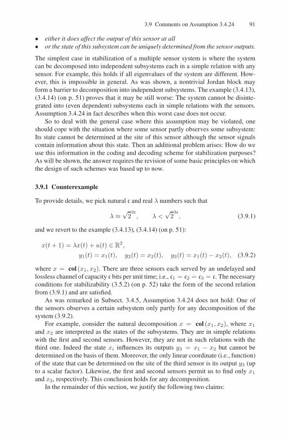
3.9 Comments on Assumption 3.4.24 91
• either it does affect the output of this sensor at all• or the state of this subsystem can be uniquely determined from the sensor outputs.
The simplest case in stabilization of a multiple sensor system is where the systemcan be decomposed into independent subsystems each in a simple relation with anysensor. For example, this holds if all eigenvalues of the system are different. How-ever, this is impossible in general. As was shown, a nontrivial Jordan block mayform a barrier to decomposition into independent subsystems. The example (3.4.13),(3.4.14) (on p. 51) proves that it may be still worse: The system cannot be disinte-grated into (even dependent) subsystems each in simple relations with the sensors.Assumption 3.4.24 in fact describes when this worst case does not occur.
So to deal with the general case where this assumption may be violated, oneshould cope with the situation where some sensor partly observes some subsystem:Its state cannot be determined at the site of this sensor although the sensor signalscontain information about this state. Then an additional problem arises: How do weuse this information in the coding and decoding scheme for stabilization purposes?As will be shown, the answer requires the revision of some basic principles on whichthe design of such schemes was based up to now.
3.9.1 Counterexample
To provide details, we pick natural c and real λ numbers such that
λ ≈√
23c, λ <
√23c, (3.9.1)
and we revert to the example (3.4.13), (3.4.14) (on p. 51):
x(t+ 1) = λx(t) + u(t) ∈ R2,
y1(t) = x1(t), y2(t) = x2(t), y3(t) = x1(t)− x2(t), (3.9.2)
where x = col (x1, x2). There are three sensors each served by an undelayed andlossless channel of capacity c bits per unit time; i.e., c1 = c2 = c3 = c. The necessaryconditions for stabilizability (3.5.2) (on p. 52) take the form of the second relationfrom (3.9.1) and are satisfied.
As was remarked in Subsect. 3.4.5, Assumption 3.4.24 does not hold: One ofthe sensors observes a certain subsystem only partly for any decomposition of thesystem (3.9.2).
For example, consider the natural decomposition x = col (x1, x2), where x1
and x2 are interpreted as the states of the subsystems. They are in simple relationswith the first and second sensors. However, they are not in such relations with thethird one. Indeed the state xi influences its outputs y3 = x1 − x2 but cannot bedetermined on the basis of them. Moreover, the only linear coordinate (i.e., function)of the state that can be determined on the site of the third sensor is its output y3 (upto a scalar factor). Likewise, the first and second sensors permit us to find only x1
and x2, respectively. This conclusion holds for any decomposition.In the remainder of this section, we justify the following two claims:

92 3 Stabilization of Multiple Sensor Systems via Limited Capacity Channels
1. The system (3.9.2) is stabilizable;2. It cannot be stabilized by a controller with the following features F.1)–F.5).
Before specifying them, we note that they are characteristic for most of the relevantcontrollers based on the design ideas presented in the literature (see, e.g., [28,89,90,135–138, 149, 184, 202, 204, 221] and the literature therein). We also recall that forthe system (3.9.2), the controller consists of three coders and a decoder.
F.1) Not only the “mode” yi but also its upper (maybe incorrect) bound δi is deter-mined at the sensor site;
F.2) The state x and these bounds in fact constitute the state of the closed-loop sys-tem, which is time-invariant;
F.3) At the decoder site, the information about the “mode” yi(t) comes to its quan-tized scaled value ei(t) = Qi[δi(t)
−1yi(t)] given by a static quantizer Qi(·)with convex level sets and the number mi of levels matching mi + 1 ≤ 2c thechannel capacity23;
F.4) The next bound δi(t+1) is determined from δi(t) and the knowledge of whetherei(t) = z;
F.5) Whenever all bounds are true δi(t) ≥ |yi(t)| ∀i, they remain true afterward.
It is clear that these features mainly concern the coding algorithm.In the remainder of this subsection, we prove claim 2. Claim 1 (i.e., stabilizability
of the system) will be justified in the next subsection.
Lemma 3.9.2. Let c ≥ 2 and a controller satisfying F.1)–F.5) be given. Then theclosed-loop system (3.9.2) is not stable. Moreover,
lim supt→∞
supx0∈Bχ
0
‖x(t)‖ =∞ (3.9.3)
for all χ > 0 and initial bounds δ0i > 0.
Proof. By F.2) and F.4), δi(t+ 1) = Di[δi(t)] whenever ei(t) 6= z. We are going toestimate Di(·) from below. Due to F.3), any quantizer Qi is related to a partition ofthe interval [−1, 1] into mi subintervals (level sets)
∆(i)1 , . . . ,∆(i)
mi.
Let α(i)j and β(i)
j denote the left and right end points of ∆(i)j , respectively. Since
mi ≤ 2c − 1, one of them has the length
β(i)ji − α(i)
ji > 2 · 2−c.
Now we pick δ > 0, set the initial bounds δ1(0) = δ2(0) = δ, δ3(0) = 2δ, and notethat all initial states from the segment
23We recall that mi is the number of the quantizer outputs different from z. So the totalnumber of outputs is mi + 1.

3.9 Comments on Assumption 3.4.24 93
S := x0 = col (δα(1)j1 + θ, δα
(2)j2 + θ) : 0 < θ ≤ 2δ2−c
give rise to common outputs for each quantizer i = 1, 2, 3 at t = 0. So they giverise to a common control u(0) = col (u1, u2). For all these states, the above initialbounds are correct. Then F.5) ensures that for i = 1, 2
δi(1) = Di[δi(0)] = Di[δ] ≥ |yi(1)| = |λxi(0) + ui|.
Here λxi(0)+ ui runs over an interval of length 2λδ2−c as x0 ranges over S. Hence
Di(δ) ≥ λδ2−c (3.9.4)
for i = 1, 2. This inequality is extended on i = 3 by putting
δ1(0) = δ3(0) = δ, δ2(0) = 2δ,
S := x0 = (δα(1)j1 + θ, δα
(1)j1 − δα
(3)j3 ) : 0 ≤ θ ≤ 2δ2−c
and retracing the above arguments.Now we suppose that (3.9.3) violates for some δ0i > 0 and χ > 0
c := supx0∈Bχ
0 ,t=0,1,...
‖x(t)‖ <∞.
By decreasing χ, one can ensure that χ < minδ01 , δ02 , 12δ
03. Then for all initial
states x0 ∈ Bχ0 , the bounds δi are correct for t = 0. Thanks to F.4) and F.5), theyremain correct for all t and common for all x0 ∈ Bχ0 . Then (3.9.4) yields
δi(t) ≥ χ(λ
2c
)t.
Here λ ≈√
23c
by (3.9.1). So δi(t) → ∞ as t → ∞. As a result, the interval[−2c, 2c] is covered by at most two intervals of the form δi(t)∆
(i)j for each i =
1, 2, 3, provided t is large enough. Since
‖x(t)‖ ≤ c⇒ |yi(t)| ≤ 2c, i = 1, 2, 3,
this and F.3) mean that for x0 ∈ Bχ0 each Qi in fact acts as a binary quantizer(i.e., that with only two outputs) at any large time. Thus the decoder receives in factno more than one bit of information about the processes with x0 ∈ Bχ0 via eachchannel. By treating three channels as one and invoking Lemma 3.5.11 (on p. 56),we arrive at the inequality λ2 ≤ 23 ⇔ λ ≤ 23/2. At the same time, c ≥ 2 and so
λ ≈√
23c> 23/2. The contradiction obtained proves the lemma. ⊓⊔
3.9.2 Stabilizability of the System (3.9.2)
Now we show that despite Lemma 3.9.2, the system (3.9.2) is yet stabilizable. Thestabilizing controller will lack the properties F.2) and F.3). It will employ a 2-periodicquantization scheme applied to not only scaled but also shifted observations.

94 3 Stabilization of Multiple Sensor Systems via Limited Capacity Channels
We offer only a sketch of the proof. This is because our objective is to highlightthe design ideas, whereas (3.9.2) is of little interest by its own right.
We equip every sensor with a coder (see Fig. 3.7). At any time, the jth coderselects a code-symbol ej(t) from the c-bits channel alphabet and sends it over thejth channel to the decoder. Furthermore, this coder computes recursively an upperbound δj(t) for the current observation
−δj(t) ≤ yj(t) < δj(t). (3.9.5)
This computation is driven by the sequence of messages sent from the jth coder tothe decoder, so that the decoder be able to compute δj(t) by itself.
Fig. 3.7. Stabilization of the system (3.9.2).
We start to consider the stabilization process since the moment (treated as t = 0)when all bounds are correct. This may be due to the knowledge of such bounds forthe initial state. Otherwise this may be achieved during a preparatory stage of thestabilization process via successive multiplying δj by a sufficiently large factor, likein Subsect. 3.8.4 (see p. 68). As will be shown, these bounds are kept true afterwardby the algorithm to be proposed. It will be designed so that the following relationsbetween the bounds δj are also kept true:
δ1(t) = δ2(t), δ3(t) = δ1(t) + δ2(t) at odd times tδ2(t) = δ1(t) + δ3(t), δ3(t) = 2δ1(t)
N at even times t, (N := 2c). (3.9.6)
Description of the Controller
The coders and decoder act in different ways at odd and even times t.At odd times, the state x(t) lies in the following square by (3.9.5):
x(t) ∈M(t) := x : −δj(t) ≤ yj < δj(t), j = 1, 2. (3.9.7)
1) By acting independently on and via their own observation and channel, respec-tively, the first and second (j = 1, 2) coders in fact apply the uniform N2-level

3.9 Comments on Assumption 3.4.24 95
quantization scheme (see Example 3.8.11 on p. 70) to the square (3.9.7) and no-tify the decoder which of the level domains contains the state (see Fig. 3.8a).Formally, for j = 1, 2, the jth coder determines which interval
[µ(j)i′ , µ
(j)i′+1), where µ
(j)i := i
2δj(t)
N, i′ = 0, . . . , N − 1,
containsyj(t) := yj(t) + δj(t)
and notifies the decoder about its serial number i′ = i(j);
Fig. 3.8(a). Uniform square quantizer. Fig. 3.8(b). Location of the state.
2) At the same time, the third coder (j = 3) does the following:a) finds which of 2N intervals
[ωi, ωi+1), where ωi := iδj(t)
N, (3.9.8)
contains yj(t);b) uniformly partitions this interval into N/2 subintervals
[ω(ν)i , ω
(ν+1)i ), ω
(ν)i := ωi + 2ν
ωi+1 − ωiN
(3.9.9)
and notifies the decoder which of them ν = 0, . . . , N/2 − 1 contains yj(t),and
c) uses the remaining bit to make the decoder aware of whether i is odd or even.
Explanation 3.9.3. In fact, the third sensor displays the orthogonal projection of thepoint x = col (x1, x2) onto the line x1 = −x2. The embedding square (3.9.7)is projected onto its diagonal. The set of the intervals (3.9.8) can be interpreted asthe uniform partition of the diagonal into 2N segments (see Fig. 3.8b). It is easy

96 3 Stabilization of Multiple Sensor Systems via Limited Capacity Channels
to check that the shadowed square from Fig. 3.8a (the quantizer level domain) isprojected onto the union of two neighboring segments. So the decoder can determinethis union from the data provided by the first and second coders. The bit from c)enables the decoder to select the segment (3.9.8) that contains the projection fromthe above two neighboring ones.
Hence except for one bit, the remaining bits available to the third coder can beused to improve the precision in location of the projection within the segment (3.9.8),which is done by b).
Remark 3.9.4. In the more formal analytical way, the above arguments look as fol-lows. It is easy to check that
(i(1) + i(2)∗ )
δ3(t)
N< y3(t) < (i(1) + i
(2)∗ + 2)
δ3(t)
N, i
(2)∗ := N − i(2) − 1.
So either i = i(1) + i(2)∗ or i = i(1) + i
(2)∗ + 1. Hence i can be found from the data
i(1), i(2) given by the first and second sensors, and the bit from c).
3). Based on the data i(1) from the first sensor, the decoder finds the strip
x : y1 ∈ −δ1(t) + [µ(1)
i(1), µ
(1)
i(1)+1)
that contains x(t). By finding i on the basis of the data from the first and secondsensors, along with the bit from 2.c), and using the data ν described in 2.b), itfinds another such strip (which is N/2-times ”narrower” than the first one)
x : y3 ∈ −δ3(t) + [ω(ν)i , ω
(ν+1)i ).
Then the decoder selects a control driving the system from the center of theintersection of the strips (the shadowed domain in Fig. 3.9a) to zero.
Fig. 3.9(a). Location of the state: the viewof the decoder.
Fig. 3.9(b). Domain transformation at anodd step.

3.9 Comments on Assumption 3.4.24 97
Explanation 3.9.5. In fact, the decoder might locate the state better by computing theshadowed domain from Fig. 3.8b. We make use of the domain from Fig. 3.9a sincethis ensures stability by employing simpler formulas.
Remark 3.9.6. By invoking (3.9.2) and (3.9.7), it is easy to check that the selectedcontrol drives the system to the state
x(t + 1) ∈M(t+ 1) := x : −ε′ ≤ y1 < ε′, −ε′′ ≤ y3 < ε′′,
where
ε′ := λδ1(t)N−1 (3.9.1)≈ δ1(t)2
3/2c2−c = δ1(t)2c/2
c≥2> δ1(t),
ε′′ := 2λδ1(t)N−2 (3.9.1)≈ 2δ1(t)︸ ︷︷ ︸
=δ3(t) by (3.9.6)
2−c/2 < δ3(t).
Thus, for one step, the domain M(t) locating the state M(t) ∋ x(t) is stretched inone direction and tightened in the other (see Fig. 3.9b).
It is easy to see that the area of the set M(t) progresses by multiplying by 2λ2
23c
per odd step. So it decreases if λ < 1√223/2c. This is a bit more restrictive than
the condition λ < 23/2c from (3.9.1). This gap can be discarded by increasing thesample period to r time units. Indeed, this “transforms” λ into λr, c into rc, and theabove condition λ < 2
32 c− 1
2 into λ < 232 c− 1
2r ≈ 23/2c for r ≈ ∞.
4). Both the jth coder and the decoder define the next number δj as the upper boundfor yj when x ranges over M(t+ 1); i.e.,
δ1(t+ 1) := λN−1δ1(t),
δ3(t+ 1) := λN−2δ3(t),
δ2(t+ 1) := λδ2(t)N−1
[1 +
2
N
].
Observation 3.9.7. This keeps (3.9.6) true at the next (even) time t := t+ 1.
Remark 3.9.8. For odd steps, the first and second coders use the available c bits inorder to increase the accuracy of the state description by 2c bits per step. Due tothe state dynamics, this is insufficient even to keep the accuracy at a given level.Indeed the required number of bits is no less than the topological entropy of thesystem at hand, which equals 2 log2 λ ≈ 3c by (3.9.1). This insufficiency can becompensated by the bits available to the third sensor. However this sensor cannotdistinguish between points lying on lines parallel to x1 = x2. So the correspondingbits can aid in refining the state description only in the perpendicular direction.
This explains why the state location domain is tightened in this direction andstretched along the above line x1 = x2. Another conclusion is that repeating of theabove scheme (where the first and second sensors supply a primary “rough” infor-mation about the state and the third sensor is used to refine it) will stretch the state

98 3 Stabilization of Multiple Sensor Systems via Limited Capacity Channels
location domain along the line x1 = x2 further and will not result in stabilization. Sothe roles of the sensors should be interchanged. This is done at the even steps. Thenthe first and third sensors supply primary data, whereas the second one refines it.
At even times, the state x(t) lies in the following parallelogram by (3.9.5):
x(t) ∈M(t) := x : −δi(t) ≤ yi < δi(t), i = 1, 3, (3.9.10)
where δ3(t) = 2δ1(t)N and δ2(t) = δ1(t) + δ3(t) by (3.9.6) (see Fig. 3.10a).
aaaaaaaaaaaaaaaa
aaaaaaaaaaaaaaaaaaaaaaaaaaaaaaaaaaaaaaaaaaaaaaaaaaaaaaaaaaaaaaaaaaaaaaaaaaaaaaaaaaaaaaaaaaaaaaaaaaaaaaaaaaaaaaaaaaaaaaaaaaaaaaaaaaaaaaaaaaaaaaaaaaaaaaaaaaaaaaaaaaaaaaaaaaaaaaaaaaaaaaaaaaaaaaaaaaaaaaaaaaaaaaaaaaaaaaaaaaaaaaaaaaaaaaaaaaaaaaaaaaaaaaaaaaaaaaaaaaaaaaaaaaaaaaaaaaaaaaaaaaaaaaaaaaaaaaaaaaaaaaaaaaaaaaaaaaaaaaaaaaaaaaaaaaaaaaaaaaaaaaaaaaaaaaaaaaaaaaaaaaaaaaaaaaaaaaaaaaaaaaaaaaaaaaaaaaaaaaaaaaaaaaaaaaaaaaaaaaaaaaaaaaaaaaaaaaaaaaaaaaaaaaaaaaaaaaaaaaaaaaaaaaaaaaaaaaaaaaaaaaaaaaaaaaaaaaaaaaaaaaaaaaaaaaaaaaaaaaaaaaaaaaaaaaaaaaaaaaaaaaaaaaaaaaaaaaaaaaaaaaaaaaaaaaaaaaaaaaaaaaaaaaaaaaaaaaaaaaaaaaaaaaaaaaaaaaaaaaaaaaaaa
Fig. 3.10(a). Location of the state: the viewof the first and third sensors.
Fig. 3.10(b). Location of the state: the viewof the decoder.
5). The operation 1) is carried out by the first and third coders j = 1, 3, and 2) isdone by the second one j = 2 with ωi altered: ωi := i 2δ2(t)N .
Explanation 3.9.9. By acting independently on and via their own observation andchannel, respectively, the first and third coders in fact apply the N2-level quantiza-tion scheme to the parallelogram (3.9.10) and notify the decoder which of the sub-parallelograms contains the state (see the shadowed parallelogram in Fig. 3.10a).
By projecting this sub-parallelogram on the line x1 = 0, the decoder can deter-mine a segment of length ∆ := 2δ2(t)
N containing the measurement y2(t) = x2(t)from the second sensor. This segment intersects at most two intervals (3.9.8) of thesame length ∆. The interval (3.9.8) found by the second coder is among these twoones. So the decoder can uniquely restore this interval by using the bit from c).
In the more formal analytical way, the above arguments look as follows. It is easyto check that i(1), i(3) ∈ [0 : N − 1] and

3.9 Comments on Assumption 3.4.24 99
−δ2(t) + 2δ2(t)N
[i(1) + 2
N+2
(N − 1− i(3) − i(1)
)]< y2(t)
< −δ2(t) + 2δ2(t)N
[i(1) + 2
N+2
(N − 1− i(3) − i(1)
)+ 1]
⇓either − δ2(t) + 2δ2(t)
N
⌊a(i(1), i(3))
⌋< y2(t)
< −δ2(t) + 2δ2(t)N
(⌊a(i(1), i(3))
⌋+ 1)
or − δ2(t) + 2δ2(t)N
(⌊a(i(1), i(3))
⌋+ 1)≤ y2(t)
< −δ2(t) + 2δ2(t)N
(⌊a(i(1), i(3))
⌋+ 2)
where
a(i(1), i(3)) :=2
N + 2
(N − 1− i(3) − i(1)
)+ i(1).
It follows that the serial number i = 1, 2 of the interval [ωi, ωi+1) (with ωi :=
i 2δ2(t)N ) containing y2(t) equals either⌊a(i(1), i(3))
⌋or⌊a(i(1), i(3))
⌋+ 1. So it can
be found by the decoder on the basis of the data i(1), i(3) from the first and thirdsensors and the information from 2.c).
So by using the data from b), the decoder can also determine the correspondingsubinterval (3.9.9) of length 4δ2(t)
N2 .
Remark 3.9.10. The definition of the quantityωi from 3) is altered at even steps sincethe projections of the quantizer level domains from Fig. 3.10a on the line x1 = 0 arearranged in a less regular way, as compared with Fig. 3.8a. In the case from Fig. 3.8a,all projections can be obtained via successive displacement of one of them by exactlythe half length. In the case from Fig. 3.10a, the displacement should be by 2
N+2×length.
6) The decoder finds a domain containing x(t) by intersecting two strips:
x : y3 ∈ −δ3(t) + [µ
(3)
i(3), µ
(3)
i(3)+1),
x : y2 ∈ −δ2(t) + [ω
(ν)i , ω
(ν+1)i )
.
Then the decoder selects a control driving the system from the center of thisdomain to zero (see Fig. 3.10b).
Remark 3.9.11. By invoking (3.9.2), it is easy to check that the selected control drivesthe system to the state
x(t+ 1) ∈M ′(t+ 1) :=x : −ε′ ≤ y3 < ε′, −ε′′ ≤ y2 < ε′′
,
where
ε′ := λδ3(t)N−1, ε′′ := 1/2[ω
(ν+1)i − ω(ν)
i ]
=2λδ2(t)
N2= λ
N + 2
N2δ3(t) ≤ 3λδ3(t)N
−1.

100 3 Stabilization of Multiple Sensor Systems via Limited Capacity Channels
The set M ′(t+ 1) is covered by the square
M(t+ 1) :=
x : |x1|, |x2| ≤ 3λ
δ3(t)
N
.
7) Both the jth coder and the decoder define the next number δj so that δ1 = δ2become the half length of the edge of M(t+ 1) and δ3 = δ1 + δ2; i.e.,
δ1(t+ 1) :=6λ
N2δ1(t),
δ2(t+ 1) :=6λ
N(N + 2)δ2(t),
δ3(t+ 1) := 6λδ3(t)N−1.
Thus the description of the stabilization process is completed.
Observation 3.9.12. For two steps, the square M(t) ∋ x(t) with the edge 2δ1(t)(where t is odd) is transformed into the square M(t+ 2) with the edge
2δ1(t)×6λ2
N3.
So the system is stabilized if
6λ2
N3< 1⇔ λ <
1√623/2c. (3.9.11)
Remark 3.9.13. The condition (3.9.11) is a bit worse than the necessary condition forstabilizability λ < 23/2c from (3.9.1). This gap can be discarded by increasing thesample period to r time units, where r is large enough. Indeed, this “transforms” λinto λr, c into rc, and the sufficient condition (3.9.11) for stabilizability into
λr < 6−12 2
32 rc ⇔ λ < 2
32 c6−
12r ≈ 23/2c for r ≈ ∞.
Thus we see that even for a very simple system, violation of Assumption 3.4.24(on p. 49) complicates the coding–decoding scheme.

4
Detectability and Output Feedback Stabilizability ofNonlinear Systems via Limited CapacityCommunication Channels
4.1 Introduction
In the previous chapter, the problem of stabilizability via limited capacity commu-nication channels was studied for linear systems. In this chapter, we consider theproblem of stabilizability for nonlinear networked systems with a globally Lipschitznonlinearity that is common in absolute stability and robust control theories; see,e.g., [144, 151, 222]. Furthermore, we obtain a criterion of detectability of a non-linear system via limited capacity communication channels. Several results on statefeedback stabilization of uncertain plants via communication channels were obtainedin [150]. The problem of local stabilization of singular points of nonlinear networkedcontrol systems was addressed in [140, 141]. Unlike [140, 141, 150], we consider amuch more difficult case of output feedback stabilization. A criterion for output feed-back stabilization of networked nonlinear systems was given in [41]. However, thesystems considered in [41] are required to be transformable into some triangularform, whereas the nonlinear systems studied in this chapter are not assumed to sat-isfy such a strong requirement. The results of this chapter are given in terms of analgebraic Riccati inequality that originates in the theory of robust and H∞ control;see, e.g., [148, 151, 174, 178–180].
It should be pointed out that unlike Chaps. 2 and 3, which considered discrete-time systems, this chapter deals with a continuous-time plant.
The remainder of the chapter is organized as follows. Section 4.2 addresses theproblem of detectability of a nonlinear system via a digital communication channel.The output feedback stabilizability problem is studied in Sect. 4.3. As an illustration,Sect. 4.4 presents simulation results on the output feedback control of a flexible jointrobotic system.
The main results of the chapter were originally published in [170]. The illus-trative example from Sect. 4.4 was first presented in the paper [172], which alsocontains an extension of the results of [170]. Moreover, further extensions of the re-sults of this chapter to the case of nonlinear systems with monotonic nonlinearitieswere obtained in [32].
A.S. Matveev and A.V. Savkin, Estimation and Control over Communication Networks,
© Birkhäuser Boston, a part of Springer Science + Business Media, LLC 200
101 doi: 10.1007/978-0-8176-4607-3_4,
9

102 4 Detectability and Stabilizability of Nonlinear Systems
4.2 Detectability via Communication Channels
In this section, we consider nonlinear continuous-time dynamical systems of theform:
x(t) = Ax(t) +B1f(z(t));
z(t) = Kx(t);
y(t) = Cx(t), (4.2.1)
where x(t) ∈ Rn is the state; z(t) ∈ Rq is a linear output; y(t) ∈ Rk is the measuredoutput; A,B1,K , and C are given matrices of the corresponding dimensions, andf(z(t)) ∈ Rp is a given continuous nonlinear vector function. We also assume thatinitial conditions of the system (4.2.1) lie in a known bounded set X0:
x(0) ∈ X0. (4.2.2)
We assume that the vector function f(·) satisfies the following globally Lipschitzcondition:
‖f(z1)− f(z2)‖2 ≤ ‖z1 − z2‖2 ∀z1, z2. (4.2.3)
The requirement (4.2.3) is a special case of a typical sector-type constraint from theabsolute stability theory; see, e.g., [144, 151, 222]. A simple common example ofsuch a constraint is a scalar nonlinearity satisfying conditions f(0) = 0 and
−1 ≤ f(z1)− f(z2)
z1 − z2≤ 1 ∀z1, z2.
In our detectability problem, a sensor measures the state x(t) and is connected tothe controller, which is at the remote location. Moreover, the only way of commu-nicating information from the sensor to that remote location is via a digital commu-nication channel that carries one discrete-valued symbol h(jT ) at time jT , selectedfrom a coding alphabet H of size l. Here T > 0 is a given period, and j = 1, 2, 3, . . ..
This restricted number l of code words h(jT ) is determined by the transmissiondata rate of the channel. For example, if µ is the number of bits that our channel cantransmit at any time instant, then l = 2µ is the number of admissible code words. Weassume that the channel is a perfect noiseless channel and that there is no time delay.
We consider the problem of estimation of the state x(t) via a digital communi-cation channel with a bit-rate constraint. Our state estimator consists of two compo-nents. The first component is developed at the measurement location by taking themeasured output y(·) and coding to the codeword h(jT ). This component will becalled “coder.” Then the codeword h(jT ) is transmitted via a limited capacity com-munication channel to the second component, which is called “decoder.” The secondcomponent developed at the remote location takes the codeword h(jT ) and producesthe estimated state x(t). This situation is illustrated in Fig. 2.1 (on p. 15).
The coder and the decoder are of the following forms:

4.2 Detectability via Communication Channels 103
Coder:
h(jT ) = Fj(y(·)|jT0
); (4.2.4)
Decoder:
x(t)|(j+1)TjT = Gj (h(T ), h(2T ), ..., h((j − 1)T ), h(jT )) . (4.2.5)
Here j = 1, 2, 3, . . ..
Definition 4.2.1. The system (4.2.1), is said to be detectable via a digital commu-nication channel of capacity l if a coder–decoder pair (4.2.4), (4.2.5) exists with acoding alphabet of size l such that
limt→∞
‖x(t)− x(t)‖∞ = 0 (4.2.6)
for any solution of (4.2.1), (4.2.2), and (4.2.3). A coder–decoder pair (4.2.4), (4.2.5)satisfying condition (4.2.6) is said to be detecting.
4.2.1 Preliminary Lemmas
We will consider the following pair of Riccati algebraic inequalities
(A− αI) TX +X(A− αI) +K TK +XB1BT1X < 0; (4.2.7)
Y A+A TY + Y B1BT1Y +K TK − α1C
TC < 0, (4.2.8)
where I is the identity square matrix, and α > 0 and α1 > 0 are given numbers.In this subsection, we prove two preliminary lemmas.
Lemma 4.2.2. Suppose that for some α > 0, a solution X > 0 of the Riccati in-equality (4.2.7) exists. Then a time T0 > 0 exists such that for any T ≥ T0 andany two solutions x1(·), x2(·) of the system (4.2.1), (4.2.2), (4.2.3), the followinginequality holds:
‖x1(t+ T )− x2(t+ T )‖∞ ≤ eαT ‖x1(t)− x2(t)‖∞ (4.2.9)
for all t ≥ 0.
Proof of Lemma 4.2.2. Let
x(t) := e−αt(x1(t)− x2(t));
φ(t) := e−αt(f(Kx1(t))− f(Kx2(t))). (4.2.10)
Then x(·), φ(·) obviously satisfy the equation
˙x(t) = (A− αI)x(t) +B1φ(t);
z(t) = Kx(t), (4.2.11)

104 4 Detectability and Stabilizability of Nonlinear Systems
and the constraint‖φ(t)‖2 ≤ ‖z(t)‖2. (4.2.12)
Then according to the strict bounded real lemma (see, e.g., Lemma 3.1.2 of [151]the system (4.2.11), (4.2.12) is quadratically stable. This implies that a time T0 > 0exists such that for any T ≥ T0 and any solution x(·) of the system (4.2.11), (4.2.12),the following inequality holds:
‖x(t+ T )‖∞ ≤ ‖x(t)‖∞ ∀t ≥ 0. (4.2.13)
The properties (4.2.13) and (4.2.10) immediately imply (4.2.9). This completes theproof of Lemma 4.2.2. ⊓⊔
Now consider the following state estimator that will be a part of our proposedcoder:
˙x(t) = (A−GC)x(t) +Gy(t) +B1f(z(t));
z(t) = Kx(t), x(0) = 0. (4.2.14)
Furthermore, we introduce the gain G by
G :=α1
2Y −1C T, (4.2.15)
where Y > 0 is a solution of (4.2.8).
Lemma 4.2.3. Suppose that for some α1 > 0, a solution Y > 0 of the Riccatiinequality (4.2.8) exists. Then a time T0 > 0 and a constant α0 > 0 exist such that
‖x(t+ T )− x(t+ T )‖∞ ≤ e−α0T ‖x(t)− x(t)‖∞ (4.2.16)
for any t ≥ 0, T > T0 and any solution of (4.2.1)–(4.2.3), (4.2.14), and (4.2.15).
Proof of Lemma 4.2.3 Let
ξ(t) := x(t) − x(t)); ζ(t) := Kξ(t);
φ(t) := f(z(t))− f(z(t)). (4.2.17)
Then ξ(·), φ(·) obviously satisfy the equation
ξ(t) = (A−GC)ξ(t) +B1φ(t) (4.2.18)
and the constraint‖φ(t)‖2 ≤ ‖ζ(t)‖2. (4.2.19)
Since Y > 0 is a solution of (4.2.8) and G is defined by (4.2.15), the matrix Y isalso a positive-definite solution of the Riccati inequality
(A−GC) TY + Y (A−GC) +K TK + Y B1BT1 Y < 0.
Therefore, according to the strict bounded real lemma (see, e.g., Lemma 3.1.2 of[151]), the system (4.2.17), (4.2.18), (4.2.19) is quadratically stable. Now the state-ment of the lemma immediately follows from quadratic stability. This completes theproof of Lemma 4.2.3. ⊓⊔

4.2 Detectability via Communication Channels 105
4.2.2 Uniform State Quantization
Our proposed coder–decoder pair uses uniform quantization of the states x of thesystem (4.2.14) in which the same number of bits is used to quantize each statevariable. The corresponding quantizer was introduced in Remark 3.8.13 (on p. 71).For the convenience of the reader, now we recall the basic formulas describing thisquantizer. Furthermore, now we consider the case where the effective quatizationdomain is an arbitrary cube, whereas only the cube with side length 2 was consideredin Remark 3.8.13.
To quantize the state space of the estimator (4.2.14), let a > 0 be a given constantand consider the set:
Ba := x ∈ Rn : ‖x‖∞ ≤ a .
The state space of the system (4.2.14) is quantized by dividing the set Ba into qn
hypercubes, where q is a specified integer. Indeed, for each i ∈ 1, 2, . . . , n, wedivide the corresponding component of the vector xi into q intervals as follows:
Ii1(a) :=
xi : −a ≤ xi < −a+
2a
q
;
Ii2(a) :=
xi : −a+
2a
q≤ xi < −a+
4a
q
;
...
Iiq(a) :=
xi : a− 2a
q≤ xi ≤ a
. (4.2.20)
Then for any x ∈ Ba, unique integers i1, i2, . . . , in ∈ 1, 2, . . . , q exist such that
x ∈ I1i1 (a)× I2
i2(a)× . . .× Inin(a).
Also, corresponding to the integers i1, i2, . . . , in, we define the vector
η(i1, i2, . . . , in) :=
−a+ a(2i1 − 1)/q−a+ a(2i2 − 1)/q
...−a+ a(2in − 1)/q
. (4.2.21)
This vector is the center of the hypercube I1i1
(a)× I2i2
(a)× . . .× Inin(a) containingthe original point x.
Note that the regions I1i1
(a)× I2i2
(a)× . . .× Inin(a) partition the region Ba intoqn regions; e.g., for n = 2 and q = 3, the region Ba would be divided into nineregions as shown in Fig. 4.1.
In our proposed coder–decoder pair, each of these regions will be assigned a codeword and the coder will transmit the code word corresponding to the current state ofthe system (4.2.14) x(jT ). The transmitted code word will correspond to the integersi1, i2, . . . , in. In order that the communication channel be able to accomplish this

106 4 Detectability and Stabilizability of Nonlinear Systems
Fig. 4.1. Uniform quantization of the state space.
transmission, the number qn of quantizer outputs should not exceed the size l of thechannel alphabet H
qn ≤ l. (4.2.22)
The above quantization of the state space of the system (4.2.14) depends on thescaling parameter a > 0. In our proposed coder–decoder pair, this parameter will bethe quantization scaling a(jT ), where j = 1, 2, . . ..
We now suppose that the assumptions of Lemmas 4.2.2 and 4.2.3 are satisfied.Then let T > 0 be a time such that the conditions (4.2.9) and (4.2.16) hold. Further-more, introduce
m0 := supx0∈X0
‖x0‖∞; a(T ) := (eαT + e−α0T )m0;
a(jT ) := eαTa((j − 1)T )
q+
(e(α−α0(j−1))T + e−α0jT )m0 ∀j = 2, 3, . . . . (4.2.23)

4.2 Detectability via Communication Channels 107
Introduce now our proposed coder–decoder pair:Coder:
h(jT ) = i1, i2, . . . , in (4.2.24)
for
(x(jT )− x(jT − 0) ∈ I1i1 (a(jT ))× I2
i2 (a(jT ))× . . .× Inin(a(jT )) ⊂ Ba(jT );
Decoder:
x(0) = 0; z(t) = Kx(t),˙x(t) = Ax(t) +B1f(z(t)) ∀t 6= jT ;
x(jT ) = x(jT − 0) + η(i1, i2, . . . , in)
for h(jT ) = i1, i2, . . . , in ∀j = 1, 2, . . . . (4.2.25)
We recall that ν(t − 0) denotes the limit of the function ν(·) at the point t from theleft. Notice that our decoder is described by a differential equation with jumps.
Also notice that equations (4.2.25) are a part of both coder and decoder, and itfollows immediately from (4.2.9), (4.2.16) and initial condition x(0) = 0 that
x(T ) ∈ Ba(T ); x(jT )− x(jT − 0) ∈ Ba(jT ) (4.2.26)
for all j = 2, 3, . . . and for any solution of (4.2.1), (4.2.2), and (4.2.3).The main requirement for our coding–decoding scheme is as follows:
q > eαT . (4.2.27)
Now we are in a position to present the main result of this section.
Theorem 4.2.4. Suppose that for some α > 0, a solution X > 0 of the Riccati in-equality (4.2.7) exists and for some α1 > 0, a solution Y > 0 of the Riccati inequal-ity (4.2.8) exists. Furthermore, suppose that for some T > 0 satisfying conditions(4.2.9), (4.2.16) and some positive integer q, the inequality (4.2.27) holds. Supposealso that the size l of the channel alphabet meets the requirement (4.2.22). Then thecoder–decoder pair (4.2.14), (4.2.15), (4.2.23), (4.2.24), (4.2.25) is detecting for thesystem (4.2.1), (4.2.2), (4.2.3).
Proof of Theorem 4.2.4. Condition (4.2.27) implies that
limj→∞
a(jT ) = 0.
Hencelimj→∞
[η(i1, i2, . . . , in)− (x(jT )− x(jT ))
]= 0,

108 4 Detectability and Stabilizability of Nonlinear Systems
where h(jT ) = i1, i2, . . . , in. This implies that
limj→∞
(x(jT )− x(jT )) = 0.
From this and Lemma 4.2.3 we obtain that
limj→∞
(x(jT )− x(jT )) = 0
for any solution of the system (4.2.1), (4.2.2), (4.2.3). Detectability now immediatelyfollows from this and (4.2.25). This completes the proof of Theorem 4.2.4. ⊓⊔
4.3 Stabilization via Communication Channels
In this section, we consider a nonlinear continuous-time dynamic system of the form:
x(t) = Ax(t) +B1f(z(t)) +B2u(t);
z(t) = Kx(t);
y(t) = Cx(t), (4.3.28)
where x(t) ∈ Rn is the state; u(t) ∈ Rm is the control input; z(t) ∈ Rq is a linearoutput; y(t) ∈ Rk is the measured output; A,B1, B2,K , and C are given matricesof the corresponding dimensions, and f(z(t)) ∈ Rp is a given continuous nonlinearvector function.
We also assume that initial conditions of the system (4.3.28) lie in a knownbounded set X0 (4.2.2). Furthermore, we suppose that the nonlinearity f(z) satis-fies the constraint (4.2.3).
We consider the problem of output feedback stabilization of the nonlinear sys-tem (4.3.28), (4.2.2), (4.2.3) via a digital communication channel with a bit-rate con-straint. Our controller consists of two components. The first component is developedat the measurement location by taking the measured output y(·) and coding to thecodeword h(jT ). This component will be called “coder.” Then the codeword h(jT )is transmitted via a limited capacity communication channel to the second compo-nent, which is called “decoder-controller.” The second component developed at a re-mote location takes the codeword h(jT ) and produces the control input u(t) wheret ∈ [jT, (j + 1)T ). This situation is illustrated in Fig. 2.2 (on p. 25), where now anonlinear plant is considered.
The coder and the decoder are of the following forms:Coder:
h(jT ) = Fj(y(·)|jT0
); (4.3.29)
Decoder-Controller:
u(t)|(j+1)TjT = Gj (h(T ), h(2T ), ..., h((j − 1)T ), h(jT )) . (4.3.30)
Here j = 1, 2, 3, . . ..

4.3 Stabilization via Communication Channels 109
Definition 4.3.1. The system (4.3.28) is said to be stabilizable via a digital commu-nication channel of capacity l if a coder–decoder-controller pair (4.3.29), (4.3.30)exists with a coding alphabet of size l such that
limt→∞
‖x(t)‖∞ = 0; limt→∞
‖u(t)‖∞ = 0 (4.3.31)
for any solution of the closed-loop system (4.3.28), (4.2.2), (4.2.3). A coder–decoderpair (4.3.29), (4.3.30) satisfying condition (4.3.31) is said to be stabilizing.
We will need the following Riccati algebraic inequality:
A TR+RA+K TK +R (B1BT1 − α2B2B
T2 )R < 0 (4.3.32)
and a related state feedback controller
u(t) = −α2
2B T
2Rx(t). (4.3.33)
Lemma 4.3.2. Suppose that for some α2 > 0, a solution R > 0 of the Riccatiinequality (4.3.32) exists. Then the closed-loop system (4.3.28), (4.2.3), (4.3.33) isglobally asymptotically stable; i.e.,
limt→∞
‖x(t)‖∞ = 0. (4.3.34)
Proof of Lemma 4.3.2 The system (4.3.28), (4.3.33) can be rewritten as
x(t) = (A− α2
2B2B
T2R)x(t) +B1f(z(t)) (4.3.35)
and the constraint (4.2.19). Since R > 0 is a solution of (4.3.32), it is also a solutionof the Riccati inequality
(A− α2
2B2B
T2R) TR+R(A− α2
2B2B
T2R)
+K TK +RB1BT1R < 0.
Therefore, according to the strict bounded real lemma (see, e.g., Lemma 3.1.2 of[151] the system (4.3.35), (4.3.33), (4.2.19) is quadratically stable. Now the state-ment of the lemma immediately follows from quadratic stability. This completes theproof of Lemma 4.3.2. ⊓⊔
Now consider the following state estimator that will be a part of our proposedcoder:
˙x(t) = (A−GC)x(t) +Gy(t)
+B1f(z(t)) +B2u(t);
z(t) = Kx(t), x(0) = 0, (4.3.36)
where the gain G is introduced by (4.2.15).

110 4 Detectability and Stabilizability of Nonlinear Systems
We now suppose that the assumptions of Lemmas 4.2.2 and 4.2.3 are satisfied.Then let T > 0 be a time such that conditions (4.2.9) and (4.2.16) hold. Furthermore,introduce a(jT ) by (4.2.23).
Introduce now our proposed coder–decoder-controller pair:Coder:
h(jT ) = i1, i2, . . . , in (4.3.37)
for (x(jT )− x(jT − 0)) ∈ I1i1 (a(jT ))× I2
i2(a(jT ))× . . .× Inin(a(jT )) ⊂ Ba(jT );Decoder-Controller:
x(0) = 0; z(t) = Kx(t);˙x(t) = Ax(t) +B1f(z(t)) +B2u(t) ∀t 6= jT ;
x(jT ) = x(jT − 0) + η(i1, i2, . . . , in)
for h(jT ) = i1, i2, . . . , in ∀j = 1, 2, . . . ;
u(t) = −α2
2B T
2Rx(t). (4.3.38)
Similar to the coder–decoder pair proposed for the detectability problem inSect. 4.2, the equations (4.3.38) are a part of both coder and decoder-controller. Itthen follows immediately from (4.2.9), (4.2.16) and initial condition x(0) = 0 that
x(T ) ∈ Ba(T ); x(jT )− x(jT − 0) ∈ Ba(jT ) (4.3.39)
for all j = 2, 3, . . . and for any solution of (4.3.28), (4.2.2), and (4.2.3).Now we are in a position to present the main result of this section.
Theorem 4.3.3. Suppose that for some α > 0, a solution X > 0 of the Riccatiinequality (4.2.7) exists; for some α1 > 0, a solution Y > 0 of the Riccati inequality(4.2.8) exists; and for some α2 > 0, a solution R > 0 of the Riccati inequality(4.3.32) exists. Furthermore, suppose that for some T > 0 satisfying conditions(4.2.9), (4.2.16) and some positive integer q, the inequality (4.2.27) holds. Supposealso that the size l of the channel alphabet meets the requirement (4.2.22). Thenthe coder–decoder-controller pair given by (4.3.36), (4.2.15), (4.2.23), (4.3.37), and(4.3.38) is stabilizing for the system (4.3.28), (4.2.2), (4.2.3).
Proof of Theorem 4.3.3 Condition (4.2.27) implies that limj→∞ a(jT ) = 0.Hence
limj→∞
[η(i1, i2, . . . , in)− (x(jT )− x(jT ))
]= 0,
where h(jT ) = i1, i2, . . . , in. This implies that
limj→∞
(x(jT )− x(jT )) = 0.
From this and Lemma 4.2.3 we obtain that
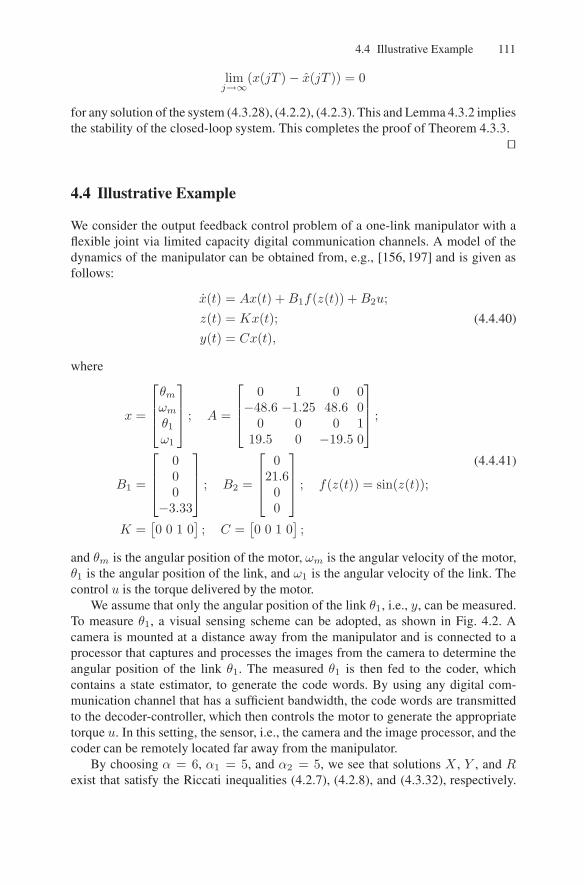
4.4 Illustrative Example 111
limj→∞
(x(jT )− x(jT )) = 0
for any solution of the system (4.3.28), (4.2.2), (4.2.3). This and Lemma 4.3.2 impliesthe stability of the closed-loop system. This completes the proof of Theorem 4.3.3.
⊓⊔
4.4 Illustrative Example
We consider the output feedback control problem of a one-link manipulator with aflexible joint via limited capacity digital communication channels. A model of thedynamics of the manipulator can be obtained from, e.g., [156, 197] and is given asfollows:
x(t) = Ax(t) +B1f(z(t)) +B2u;
z(t) = Kx(t);
y(t) = Cx(t),
(4.4.40)
where
x =
θmωmθ1ω1
; A =
0 1 0 0−48.6 −1.25 48.6 0
0 0 0 119.5 0 −19.5 0
;
B1 =
000
−3.33
; B2 =
021.600
; f(z(t)) = sin(z(t));
K =[0 0 1 0
]; C =
[0 0 1 0
];
(4.4.41)
and θm is the angular position of the motor, ωm is the angular velocity of the motor,θ1 is the angular position of the link, and ω1 is the angular velocity of the link. Thecontrol u is the torque delivered by the motor.
We assume that only the angular position of the link θ1, i.e., y, can be measured.To measure θ1, a visual sensing scheme can be adopted, as shown in Fig. 4.2. Acamera is mounted at a distance away from the manipulator and is connected to aprocessor that captures and processes the images from the camera to determine theangular position of the link θ1. The measured θ1 is then fed to the coder, whichcontains a state estimator, to generate the code words. By using any digital com-munication channel that has a sufficient bandwidth, the code words are transmittedto the decoder-controller, which then controls the motor to generate the appropriatetorque u. In this setting, the sensor, i.e., the camera and the image processor, and thecoder can be remotely located far away from the manipulator.
By choosing α = 6, α1 = 5, and α2 = 5, we see that solutions X , Y , and Rexist that satisfy the Riccati inequalities (4.2.7), (4.2.8), and (4.3.32), respectively.

112 4 Detectability and Stabilizability of Nonlinear Systems
Motor
CoderDecoder/
Controller
Camera & Image Processor
Flexible Joint
Link
Communication Channel
Fig. 4.2. Schematic of the vision-based control system.
The respective T0 values in Lemmas 4.2.2 and 4.2.3 are 0.94 and 0.91, and the valueα0 in (4.2.16) is 3.1. Therefore, we choose the sampling period T = 1.0 secondso that both inequalities (4.2.9) and (4.2.16) hold. As for the value q, we pickedq = 2001 and this value satisfies the inequality (4.2.27); i.e., q > eαT .
By using (4.2.15) and (4.3.33), the corresponding state estimator gain and controllaw are
G =[0.85 1.13 0.04 1.39
] T × 103;
u(t) =[−2.05 −0.36 −1.28 −0.90
]x(t).
(4.4.42)
For simulation purposes, the initial value of x is chosen as x(0) = [1 1 1 1] T,and the value m0 is defined as m0 = 5. Finally, a simulation result is shown inFigs. 4.3 and 4.4, and it agrees with the conditions (4.3.31).

4.4 Illustrative Example 113
0 1 2 3 4 5 6 7 8 9 10−2.5
−2
−1.5
−1
−0.5
0
0.5
1
1.5
Time (sec)
x1
x2
x3
x4
Fig. 4.3. Evolution of the state x(t).
0 1 2 3 4 5 6 7 8 9 10−1
−0.5
0
0.5
1
1.5
2
Time (sec)
Con
trol
u
Fig. 4.4. Evolution of the control input u(t).

5
Robust Set-Valued State Estimation via LimitedCapacity Communication Channels
5.1 Introduction
In this chapter, we consider the problem of robust state estimation via a limited ca-pacity digital communication channel. Many recent advances in the area of robustcontrol system design assume that the system to be controlled is modeled as an un-certain system; e.g., see [46, 148, 151]. There are many different types of uncertainsystem models. The class of time-varying uncertain systems considered in this chap-ter contains uncertainty that is defined by a certain integral quadratic constraint. Thisclass of uncertain systems originated in the work of Yakubovich on absolute stabilitytheory (see, e.g., [222, 223]) and is a particularly rich uncertainty class allowing fornonlinear, time-varying, dynamic uncertainties. Furthermore, a number of new ro-bust control system design methodologies have recently been developed for uncertainsystems with integral quadratic constraints; e.g., see [148, 151, 174, 178–180, 182].In this chapter, we adopt the approach to the robust state estimation problem pro-posed in [181] (also, see [148, 183]). Reference [181] builds on the deterministicinterpretation of Kalman filtering presented in [21]. This deterministic approach toKalman filtering also forms the launching point for the results of this chapter. As inthe previous chapter, we consider the case of continuous-time plants.
In [21], the following deterministic state estimation problem is considered: Givenoutput measurements from a time-varying linear system with noise inputs subjectedto an L2 norm bound, find the set of all states consistent with these measurements.Such a problem is referred to as a set-valued state estimation problem. The solutionto this problem was found to be an ellipsoid in the state space that is defined bythe standard Kalman filter equations. Thus, the results of [21] give an alternativeinterpretation of the standard Kalman filter. In [148,181,183] the results of [21] wereextended to the case of uncertain systems with integral quadratic constraints. In thischapter, we employ the set-valued approach to the state estimation problem and thedeterministic interpretation of Kalman filtering from [148,181] in the situation wherestate estimation is to be performed via a limited capacity communication channel.
In such a context, state estimation results for linear systems with bounded orGaussian noise were obtained in [45, 133, 220]. Some state estimation scheme rel-
A.S. Matveev and A.V. Savkin, Estimation and Control over Communication Networks,
© Birkhäuser Boston, a part of Springer Science + Business Media, LLC 200
115 doi: 10.1007/978-0-8176-4607-3_5,
9

116 5 Robust Set-Valued State Estimation via Communication Channels
evant to the problem of stabilization via a limited capacity communication channelwas proposed in [70]. Also, in [70], the case of a linear system without uncertaintyover an infinite time interval was considered.
The remainder of the chapter is organized as follows. In Sect. 5.2, we introducethe class of uncertain systems under investigation. Section 5.3 presents the statementof the optimal robust state estimation problem and some preliminary results on ro-bust set-valued state estimation originally published in [181]. In Sect. 5.4, we give asolution to an optimal state estimation problem via limited capacity digital communi-cation channels for the class of uncertain systems under consideration. Furthermore,in Sect. 5.5, we propose a suboptimal state estimation algorithm that is computation-ally nonexpansive and easily implementable in real time. Finally, in Sect. 5.6, proofsof two lemmas on set-valued state estimation can be found.
The main results presented in this chapter originally appeared in the paper [100].An analog of these results for systems without uncertainty was published before thatin [184], where some of the main ideas of the chapter were introduced. Also, someversions of technical results on robust state estimation that are used in this chapterwere first obtained in [174, 176, 181, 183]. The uncertain system framework of thischapter was presented in the monographs [148, 151, 174]. In [99], the results of thischapter were successfully applied to the problem of precision missile guidance basedon radar/video sensor fusion. An extension of the results of the chapter can be foundin [33].
5.2 Uncertain Systems
In designing robust state estimation systems, one must specify the class of uncertain-ties against which the state estimator is to be robust. The most common approach incontrol engineering is to begin with a plant model that not only models the nominalplant behavior but also models the type of uncertainties that are expected. Such aplant model is referred to as an uncertain system.
There many various types of uncertain system models; e.g., see [46]. In thischapter, we deal with uncertain plants with uncertainties satisfying so-called inte-gral quadratic constraints.
5.2.1 Uncertain Systems with Integral Quadratic Constraints
Consider the time-varying uncertain system defined over the finite time interval[0, NT ] :
x(t) = A(t)x(t) +B(t)w(t);
z(t) = K(t)x(t);
y(t) = C(t)x(t) + v(t), (5.2.1)
where N > 0 is an integer; T > 0 is a given constant; x(t) ∈ Rn is the state;w(t) ∈ Rp and v(t) ∈ Rl are the uncertainty inputs; z(t) ∈ Rq is the uncertainty

5.2 Uncertain Systems 117
output and y(t) ∈ Rl is the measured output; and A(·), B(·),K(·), and C(·) arebounded piecewise continuous matrix functions.
The uncertainty in (5.2.1) is described by an equation of the form:[w(t)v(t)
]=
[φ1(t, z(t))φ2(t, z(t))
], (5.2.2)
where the following integral quadratic constraint is satisfied.Let X0 = XT
0 > 0 be a given matrix, x0 ∈ Rn be a given vector, d > 0 be agiven constant, and Q(·) = Q(·) T and R(·) = R(·) T be given bounded piecewisecontinuous matrix weighting functions satisfying the following condition: A constantδ > 0 exists such thatQ(t) ≥ δI, R(t) ≥ δI for all t . For a given finite time interval[0, s], we will consider the uncertainty inputsw(·) and v(·) and initial conditionsx(0)such that
(x(0)− x0)TX0(x(0)− x0) +
∫ s
0
(w (t)
TQ (t)w (t) + v (t)
TR (t) v (t)
)dt
≤ d+
∫ s
0
‖z (t)‖2 dt. (5.2.3)
The uncertainty input in (5.2.2) can be regarded as the feedback interconnectionwith the uncertainty output z(t) as shown in Fig. 5.1. The inequality (5.2.3) givessome constraint on the sizes of the uncertainty inputs w(·), v(·) and on the size ofuncertainty in the initial condition.
Nominal system
Fig. 5.1. Uncertain system.
This class of uncertainties was introduced in the theory of absolute stability byYakubovich (e.g., see [222]), and extensively studied in the theory of robust control(e.g., see [148, 151, 174, 178–181]).
5.2.2 Uncertain Systems with Norm-Bounded Uncertainty
An important class of uncertain systems satisfying the integral quadratic constraint(5.2.3) consists of linear uncertain systems with uncertainties satisfying a standardnorm-bounded constraint. In this case, the uncertain system is described by the rela-tionships

118 5 Robust Set-Valued State Estimation via Communication Channels
x = [A(t) +B(t)∆1(t)K(t)]x(t);
y = [C(t) +∆2(t)K(t)]x (t) , (5.2.4)
where ∆1(t), ∆2(t) are uncertainty matrices such that∥∥∥∥∆1(t)∆2(t)
∥∥∥∥ ≤ 1 (5.2.5)
for all t.Also, the initial conditions are required to satisfy the following inequality:
(x (0)− x0)TX0 (x (0)− x0) ≤ d. (5.2.6)
The block-diagram of such a system is shown in Fig. 5.2.
NominalSystem
+
Fig. 5.2. Uncertain system with norm-bounded uncertainty.
To verify that such uncertainty is admissible for the uncertain system (5.2.1),(5.2.3), let w(t) := ∆1(t)K(t)x(t), v(t) := ∆2(t)K(t)x(t), and z(t) := K(t)x(t).Then the condition (5.2.3) is satisfied with Q(·) ≡ I and R(·) ≡ I.
5.2.3 Sector-Bounded Nonlinearities
This class of uncertainties arose from the celebrated theory of absolute stability; e.g.,see [144, 222, 224]. Consider the time-invariant uncertain system (5.2.1) with scalaruncertainty input w and uncertainty output z, and the uncertainty is described by theequation
w(t) = φ(z(t)), (5.2.7)
where φ(·) : R→ R is an uncertain nonlinear mapping.This system is represented in the block diagram shown in Fig. 5.3.We will suppose that the uncertain nonlinearity φ(·) satisfies the following sector
bound (e.g., see [144]):
0 ≤ φ(z)
z≤ k, (5.2.8)

5.3 State Estimation Problem 119
-
-
zw
y
φ(·)
System
Nominal
Fig. 5.3. Uncertain system with a single nonlinear uncertainty.
where 0 < k ≤ ∞ is a given constant associated with the system. Using the changeof variables z = k/2z, w = φ(2/kz)− z, this system is transformed into the system
x(t) = (A+k
2BK)x(t) +Bw(t);
z(t) =k
2Kx(t).
The bound (5.2.8) on the uncertainty in this system then becomes a standard boundon the norm of the uncertainty input:
|w(t)| ≤ |z(t)|. (5.2.9)
This observation motivates us to think of sector bounded uncertainty as a special caseof norm-bounded uncertainty.
Remark 5.2.1. Notice that the nonlinear system with a nonlinearity satisfying theglobally Lipschitz condition (4.2.3) (on p. 102) that was studied in Chap. 4 is aspecial case of the system with norm-bounded nonlinearity.
5.3 State Estimation Problem
We consider the set-valued state estimation problem for the system (5.2.1), (5.2.3)that can be stated as follows. Let y(t) = y0(t) be a fixed measured output of theuncertain system (5.2.1), and let s ∈ [0, NT ] be given time. Then find the corre-sponding set Xs [x0, y0 (·) |s0, d] of all possible states x(s) at time s for the uncertainsystem (5.2.1), with the uncertainty input and initial states satisfying the constraint(5.2.3). The state estimator will be defined by the differential equation

120 5 Robust Set-Valued State Estimation via Communication Channels
˙x(s) = [A(s) + P (s) [K(s) TK(s)− C(s) TR(s)C(s)]] x(s)
+ P (s)C(s) TR(s)y(s), x(0) = x0, (5.3.10)
where P (s) is the solution of the following Riccati differential equation:
P (s) = A(s)P (s) + P (s)A(s) T
+ P (s)[K (s)
TK(s)− C(s) TR(s)C(s)
]P (s) +B(s)Q(s)−1B(s) T,
P (0) = X−10 . (5.3.11)
Definition 5.3.1. The uncertain system (5.2.1), (5.2.3) is said to be robustly observ-able on [0, NT ], if for any vector x0 ∈ Rn, any time s ∈ [0, NT ], any constantd > 0, any fixed measured output y(t) = y0(t), the setXs [x0, y0(·)|s0, d] is bounded.
The following result offers an exhaustive criterion for the system to be robustlyobservable.
Lemma 5.3.2. Let X0 = X T0 > 0 be a given matrix, and let Q(·) = Q(·) T and
R(·) = R (·) T be given matrix functions such that Q(·) ≥ δI, R (·) ≥ δI , whereδ > 0. Consider the system (5.2.1) and the constraint (5.2.3) . Then the followingstatements hold:
(i) The system (5.2.1), (5.2.3) is robustly observable on [0, NT ] if and only if thesolution P (·) to the Riccati equation (5.3.11) is defined and positive-definite onthe interval [0, NT ] ;
(ii) If the system (5.2.1), (5.2.3) is robustly observable on [0, NT ], then for anyvector x0 ∈ Rn, any s ∈ [0, NT ], any constant d > 0, and any fixed measuredoutput y(t) = y0(t), the set Xs [x0, y0 (·) |s0, d] of all possible states x(s) attime s is given by
Xs [x0, y0 (·) |s0, d]
=
xs ∈ R
n :(xs − x(s)) T
P (s)−1 (xs − x(s))≤ d+ ρs [y0 (·)]
, (5.3.12)
where
ρs [y0 (·)]
:=
∫ s
0
[‖K(t)x(t)‖2 − (C(t)x(t)− y0(t)) T R(t) (C(t)x(t)− y0(t))
]dt.
(5.3.13)
The proof of Lemma 5.3.2 is given in Sect. 5.6.
Remark 5.3.3. The state estimator defined by (5.3.10) and (5.3.11) is of the sameform as the state estimator, which occurs in the output feedback H∞ control prob-lem; e.g., see [91, 130].

5.3 State Estimation Problem 121
In our state estimation problem, the state x(s) should be estimated. Now considerthe case where the only way of communicating information from the measured out-put y is via a digital communication channel with the following bit-rate constraint.This channel can transmit codesymbols h = hk at the time instants of the form kT .The channel gives a limited finite number of admissible codesymbols h. This re-stricted number of codesymbols h is determined by the data rate of the channel. IfN is the number of admissible codesymbols, thenN = 2l, where l is the number ofbits that our channel can transmit at any time kT . We assume that the channel is aperfect noiseless channel and that there is no time delay in the channel. In this chap-ter, we propose algorithms for state estimation via a digital communication channelwith the above bit-rate constraint. Our algorithms consist of two components. Thefirst component is developed at the measurement location by taking the measuredoutput signal y and coding it into the codesymbol hk at time kT . This componentwill be called coder. Then the codesymbol hk is transmitted via a limited capacitycommunication channel to the second component, which is called decoder. The de-coder takes the codesymbols hi, i ≤ k and produces the estimated state x(kT ) thatis an approximation of the center of all possible states of the system at time kT . Thissituation is illustrated in Fig. 5.4.
UncertainSystem Coder Decoder
channel
Fig. 5.4. State estimation via digital communication channel.
The coder and decoder are defined by the following equations:Coder:
h (kT ) = Fk(x0, d, y (·) |kT0
); (5.3.14)
Decoder:x (kT ) = Gk (x0, d, h0, h1, . . . , hk) . (5.3.15)
We recall that ‖x‖∞ := maxi|xi| for x = col [x1, x2, . . . , xn].
Definition 5.3.4. Consider the system (5.2.1), (5.2.3) with a given d > 0. Let ǫ > 0be a given constant, and let N > 0 and 0 < M ≤ N be given integers. The coder–decoder pair (5.3.14), (5.3.15) is said to solve the state estimation problem via adigital communication channel with the admissible number of codesymbols N onthe time interval [MT,NT ] with the precision level ǫ if
‖x(kT )− x(kT )‖∞ ≤ ǫ (5.3.16)
for all x0, y (·) , k = M,M + 1, . . . , N. Here x(kT ) is defined by (5.3.10).Moreover, if the constant ǫ in (5.3.16) is the infimum over all precision levels
that can be achieved by coder–decoder pairs of the form (5.3.14), (5.3.15) with the

122 5 Robust Set-Valued State Estimation via Communication Channels
admissible number of codesymbols N , the coder–decoder pair is said to be opti-mal for the state estimation problem via a digital communication channel with theadmissible number of codesymbolsN on the time interval [MT,NT ].
Our problem is to design an optimal coder–decoder pair.
5.4 Optimal Coder–Decoder Pair
In this section, we construct an optimal coder–decoder pair for the problem of stateestimation with bit-rate constraints. To formulate the main results of the section,we need to introduce the concept of strong robust observability that is close to theconcept of uniform robust observability from Chap. 15.
Definition 5.4.1. Consider the uncertain system (5.2.1), (5.2.3). Let Xs[d] be the setof all possible states x(s) at time s ∈ (0, NT ], defined by (5.3.10) with all possibleinitial conditions x0 ∈ Rn and all possible measured outputs y0(·) of the system(5.2.1), (5.2.3). The uncertain system (5.2.1), (5.2.3) is said to be strongly, robustlyobservable on [0, NT ] if it is robustly observable and for any time s ∈ (0, NT ] andconstant d > 0, the set Xs[d] is bounded.
Consider the following Riccati equation:
− X(s) = A(s) TX(s) +X(s)A(s)
−X(s)B(s)R−1(s)B(s) TX(s)−K(s) TK(s), X(0) = 0, (5.4.17)
whereA(t) := A(t) + P (t)K(t) TK(t) (5.4.18)
andB(t) := −P (t)C(t) TR(t). (5.4.19)
Lemma 5.4.2. The uncertain system (5.2.1), (5.2.3) is strongly, robustly observableon [0, NT ] if and only if the solution P (·) to the Riccati equation (5.3.11) is de-fined and positive-definite on [0, NT ] and the solution X(·) to the Riccati equation(5.4.17) is defined on [0, NT ] and positive-definite on (0, NT ]. Furthermore, if thesystem (5.2.1), (5.2.3) is strongly, robustly observable, then the set Xs[d] is given by
Xs[d] = xs ∈ Rn : x T
sX(s)xs ≤ d. (5.4.20)
The proof of Lemma 5.4.2 is given in Sect. 5.6.
Definition 5.4.3. Let X ⊂ Rn be a convex bounded set and N > 0 be a giveninteger. Furthermore, assume that X is partitioned into N nonintersecting sub-sets I1, I2, . . . , IN equipped with points η1 ∈ I1, . . . , ηN ∈ IN . The collectionV [X,N ] = I1, . . . , IN , η1, . . . , ηN is called an l∞ Voronoi structure on the set X
if ‖x− ηi‖∞ ≤ ‖x− ηs‖∞ for any i = 1, . . . ,N , any x ∈ Ii and any s 6= i.

5.5 Suboptimal Coder–Decoder Pair 123
Notation 5.4.4. Let V [X,N ] be an l∞ Voronoi structure. Then
D(V [X,N ]) := supi=1,...,N , x∈Ii
‖x− ηi‖∞. (5.4.21)
Definition 5.4.5. Let X be a given convex bounded set andN > 0 be a given integer.Then V [X,N ] is said to be an optimal l∞ Voronoi structure on X if D(V [X,N ]) ≤D(V∗[X,N ]) for any other l∞ Voronoi structure V∗[X,N ].
It is obvious that an optimal l∞ Voronoi structure exists on any convex boundedset. Constructing optimal Voronoi structures has been the subject of much research inthe field of vector quantization theory and computational geometry; see, e.g., [23,62].
The Coder–Decoder Pair
Let Vk[XkT [d],N ] = Ik1 , . . . , IkN , ηk1 , . . . , ηkN be the l∞ optimal Voronoistructure on the set XkT [d] defined by (5.4.20), where k = M,M + 1, . . . , N . Weare now in a position to describe our proposed optimal coder–decoder pair of theform (5.3.14), (5.3.15) associated with these structures.
Let x(0) = x0. For any k = M,M + 1, . . . , N , we consider (5.3.10) on[(k − 1)T, (kT )]. Then, for all k = M,M + 1, . . . , N , we define our coder–decoderpair as follows:Coder:
h(k) = i if x(k) ∈ Iki ⊂ XkT [d]; (5.4.22)
Decoder:x(kT ) = ηki if h(k) = i. (5.4.23)
Now we are in a position to present the main result of this chapter.
Theorem 5.4.6. Consider the uncertain system (5.2.1), (5.2.3). Let d > 0 be a givenconstant, and N > 0 and 0 < M ≤ N be given integers. Suppose that this systemis strongly, robustly observable and that the sets XkT [d] are defined by (5.4.20).
Then the coder–decoder pair (5.4.22), (5.4.23) is optimal for the state estima-tion problem via a digital communication channel with the admissible number ofcodesymbolsN on the time interval [MT,NT ].
Proof. According to Theorem 5.4.2, strong, robust observability implies that XkT [d]is the set of all possible x(kT ). Furthermore, it follows from Definition 5.4.5 that thecoding scheme that is based on a Voronoi optimal structure gives an optimal stateestimate. This completes the proof of this theorem. ⊓⊔
5.5 Suboptimal Coder–Decoder Pair
In the previous section, we proposed an optimal coder–decoder pair. The result wasgiven in terms of Voronoi structures. However, this method is computationally ex-pensive. In this section, we describe another state estimation algorithm that is notoptimal but well suited to real time implementation.

124 5 Robust Set-Valued State Estimation via Communication Channels
In this section, we propose a coder–decoder pair that uses the uniform quan-tization of the estimated states introduced in the two previous chapters. Also, thequantization parameters may be updated at every instant time kT .
To quantize the state space of (5.3.10), let a(k) > 0 be a given number and con-sider the set Ba(k) := x(kT ) ∈ Rn : |xi(kT )| ≤ a(k) ∀i . We propose to quan-tize each state component xi(kT ) by means of q(k) intervals, where q(k) is a spec-ified integer. Therefore, for n-dimensional state, the set Ba(k) will be divided intoq(k)n hypercubs. For each i ∈ 1, 2, . . . , n , we divide the corresponding compo-nent of the state vector xi(kT ) into q(k) intervals as follows:
Ii1(a(k)) :=
xi(kT ) : −a(k) ≤ xi(kT ) < −a(k) +
2a(k)
q(k)
;
Ii2(a(k)) :=
xi(kT ) : −a(k) +
2a(k)
q(k)≤ xi(kT ) < −a(k) +
4a(k)
q(k)
;
...
Iiq(k)(a(k)) :=
xi(kT ) : a(k)− 2a(k)
q(k)≤ xi(kT ) ≤ a(k)
. (5.5.24)
Then for any x(kT ) ∈ Ba(k), unique integers
i1 ∈ 1, 2, . . . , q(k) , i2 ∈ 1, 2, . . . , q(k) , . . . , in ∈ 1, 2, . . . , q(k)
exist such that
x(kT ) ∈ I1i1(a(k))× I
2i2(a(k)) × . . .× I
nin(a(k)). (5.5.25)
Also, corresponding to the integers i1, i2, . . . , in, we define the vector
η (i1, i2, . . . , in) :=
−a(k) + a(k)(2i1 − 1)/q(k)−a(k) + a(k)(2i2 − 1)/q(k)
...−a(k) + a(k)(2in − 1)/q(k)
. (5.5.26)
This vector is the center of the hypercube
I1i1(a(k))× I
2i2(a(k))× . . .× I
nin(a(k))
containing the original point x(kT ).Note that the regions I
1i1
(a(k))× I2i2
(a(k))× . . .× Inin
(a(k)) partitionBa(k) intoq(k)n regions.
In the proposed coder–decoder pair, each region will be represented by a codesym-bol, and the codesymbol corresponding to the vector x(kT ) will be transmitted via alimited capacity channel.
The Coder–Decoder Pair
We are now in a position to describe our proposed coder–decoder pair of the form(5.3.14), (5.3.15).

5.5 Suboptimal Coder–Decoder Pair 125
Let x(0) = x0. For any k = M,M + 1, . . . , N , we consider (5.3.10) on[(k − 1)T, (kT )]. Then, for all k = M,M + 1, . . . , N , we define our coder–decoderpair as follows:Coder:
h(k) := i1, i2, . . . , infor x(k) ∈ I
1i1(a(k))× I
2i2(a(k)) × . . .× I
nin(a(k)) ⊂ Ba(k); (5.5.27)
Decoder:
x(kT ) = η (i1, i2, . . . , in) for h(k) = i1, i2, . . . , in . (5.5.28)
Here the vector η (i1, i2, . . . , in) is defined in (5.5.26).The block-diagram of the uncertain system with a suboptimal coder–decoder pair
is shown in Fig. 5.5.
Stateestimator
Quantizer
Decoder
Nominal system
Coder
chan
nel
Fig. 5.5. Uncertain system with the suboptimal coder–decoder pair.
Remark 5.5.1. It should be pointed out that by our construction, the state estimatex(k) necessarily belongs to Ba(k).
Now we are ready to present the main result of the section. This will require thefollowing notation.

126 5 Robust Set-Valued State Estimation via Communication Channels
Notation 5.5.2. Let Z(·) := X(·)−1, where X(·) is the solution to (5.4.17). Letzij(·) be the corresponding element of the matrix Z(·). Then we define a constantci(k) > 0 by the following equation:
ci(k) :=√zii(kT ) for all i = 1, 2, . . . , n, k = M,M + 1, . . . , N. (5.5.29)
Note that zii(kT ) > 0 for all i, t > 0 because Z(t) is positive-definite.
Theorem 5.5.3. Consider the uncertain system (5.2.1), (5.2.3). Let d > 0 , ǫ > 0 begiven constants,N > 0 and 0 < M ≤ N be given integers. Suppose that this systemis strongly, robustly observable and
ci(k)√d
q(k)≤ ǫ, (5.5.30)
for all i = 1, 2, . . . , n and k = M,M + 1, . . . , N . Then the coder–decoder pair(5.5.27), (5.5.28) with
a(k) := maxi=1,...,n
ci(k)√d (5.5.31)
solves the state estimation problem via a digital communication channel with theadmissible number of codesymbols q(k)n ≤ N on the time interval [MT,NT ] withthe precision level ǫ.
Proof. We will prove that x(kT ) ∈ Ba(k) and inequality (5.3.16) holds for anyk = M,M+1, . . . , N . Indeed, let x(·) be a solution of the system (5.2.1) with someuncertainty input w(·) and v(·) satisfying (5.2.3), and let x(·) be the correspondingestimated state. It follows from the strong, robust observability and Theorem 5.4.2that the ellipsoid (5.4.20) is the set of all possible estimated states x(s). Thus wehave that
‖x(kT )‖∞ ≤ maxi=1,...,n
ci(k)√d. (5.5.32)
Therefore, x(kT ) ∈ Ba(k) with a(k) defined by (5.5.31). Now the condition (5.3.16)follows from (5.5.30) with a suitable q(k). This completes the proof of the theorem.
Remark 5.5.4. Notice that in [100], a slightly more general result was obtained. Acoder–decoder pair from [100] uses non-uniform quantization of the estimated statesin which different numbers of bits may be used to quantize various state variables.In this chapter, for the sake of simplicity, we consider a coder–decoder pair that isbased on uniform quantization.
5.6 Proofs of Lemmas 5.3.2 and 5.4.2
Proof of Lemma 5.3.2. Statement (i): Necessity. In this case, we must establish theexistence of a positive-definite solution to the Riccati equation (5.3.11). This willbe achieved by showing that the cost function in a corresponding linear quadraticoptimal control problem is bounded from below.

5.6 Proofs of Lemmas 5.3.2 and 5.4.2 127
Given a measured output y0(·), we have by the definition of Xs[x0, y0(·)|s0, d],that xs ∈ Xs[x0, y0(·)|s0, d] if and only if there exist vector functions x(·), w(·) andv(·) satisfying equation (5.2.1) and such that x(s) = xs, the constraint (5.2.3) holds,and
y0(t) = C(t)x(t) + v(t) (5.6.33)
xs∈Xs[x0, y0(·)|s0, d]if and only if an input w(·) ∈ L2[0, s] exists such that
J [xs, w(·)] ≤ d, (5.6.34)
where J [xs, w(·)] is defined by
J [xs, w(·)] ∆= (x(0)− x0)TX0(x(0)− x0)
+
∫ s
0
(w(t) TQ(t)w(t) − x(t) TK(t) TK(t)x(t)+(y0(t)− C(t)x(t)) TR(t)(y0(t)− C(t)x(t))
)dt (5.6.35)
and x(·) is the solution to (5.2.1) with the inputw(·) and boundary condition x(s) =xs.
Now consider the functional (5.6.35) with x0 = 0 and y0(·) ≡ 0. In this case, Jis a homogeneous quadratic functional with an end-point cost term. Also, considerthe set Xs[0, 0, 1] corresponding to x0 = 0, y0(·) ≡ 0 and d = 1. Since Xs[0, 0, 1]is bounded, a constant hs > 0 exists such that all vectors xs ∈ Rn with ‖xs‖ = hsdo not belong to the set Xs[0, 0, 1]. Hence,
J [xs, w(·)] > 1 (5.6.36)
for all xs ∈ Rn such that ‖xs‖ = hs and for all w(·) ∈ L2[0, s]. Since, J is a homo-geneous quadratic functional, we have J [axs, aw(·)] = a2J [xs, w(·)] and (5.6.36)implies that
infw(·)∈L2[0,s]
J [xs, w(·)] > 0 (5.6.37)
for all s ∈ [0, T ] and all xs 6= 0.The problem of minimizing the functional from (5.6.37) subject to the constraint
defined by the system (5.2.1) is a linear quadratic optimal control problem in whichtime is reversed. In this linear quadratic optimal control problem, a sign indefinitequadratic cost function is considered. Using a known result from the linear quadraticoptimal control theory, we conclude that the condition (5.6.37) implies that thereexists a solution Ξ(·) to the Riccati equation
− Ξ(s) = Ξ(s)A(s) +A(s) TΞ(s) +Ξ(s)B(s)Q(s)−1B(s) TΞ(s)
+K(s) TK(s)− C(s) TR(s)C(s) (5.6.38)
with the initial condition Ξ(0) = X0; e.g., see p. 23 of [34]. Furthermore, thissolution is positive-definite on [0, T ]. From this, it follows that the solution to the
for all t ∈ [0, s]. Substitution of (5.6.33) into (5.2.3) implies that

128 5 Robust Set-Valued State Estimation via Communication Channels
Riccati equation (5.3.11) is given by P (·) := Ξ(·)−1. This completes the proof ofthis part of the lemma.
Statement (ii) and the sufficiency part of statement (i). We have shown abovethat xs ∈ Xs[x0, y0(·)|s0, d] if and only if an input w(·) ∈ L2[0, s] exists such thatthe condition (5.6.34) holds for the functional (5.6.35). Now consider the followingminimization problem:
minw(·)∈L2[0,s]
J [xs, w(·)], (5.6.39)
where the minimum is taken over all x(·) and w(·) connected by (5.2.1) with theboundary condition x(s) = xs. This problem is a linear quadratic optimal trackingproblem in which the system operates in reverse time. The solution to this trackingproblem is well known (e.g., see [87]). Indeed if the solution to the Riccati equation(5.3.11) exists, then the matrix function Ξ(·) = P (·)−1 > 0 is the solution to theRiccati equation (5.6.38) with initial condition Ξ(0) = X0. From this, it followsthat the minimum in (5.6.39) is achieved for any x0 and any y0(·). Furthermore asin [21], we can write
minw(·)∈L2[0,s]
J [xs, w(·)] = (xs − x(s)) TΞ(s)(xs − x(s))− ρs,
where ρs is defined as in (5.3.13) and x(s) is the solution to (5.3.10) with the initialcondition x(0) = x0. From this we can conclude that the set
Xs[x0, y0(·)|s0, d] = xs ∈ Rn : min
w(·)∈L2[0,s]J [xs, w(·)] ≤ d
is given by (5.3.12). This completes the proof of the lemma. ⊓⊔Proof of Lemma 5.4.2. Necessity. It is obvious that strong robust observability
implies robust observability. Therefore, according to Lemma 5.3.2, the solution P (·)to the Riccati equation (5.3.11) is defined and positive-definite on [0, NT ]. We nowprove that the solutionX(·) to the Riccati equation (5.4.17) is defined on [0, NT ] andpositive-definite on (0, NT ]. It is obvious from (5.3.12) that the setXs [x0, y0(·)|s0, d]is not empty if and only if
d+ ρs [y0 (·)] ≥ 0, (5.6.40)
where ρs [y0 (·)] is defined by (5.3.13). Thus we can compose the following con-straint is satisfied by all solutions to the linear system (5.3.10):∫ s
0
[−‖K(t)x(t)‖2 + (C(t)x(t)− y0(t)) T
R(t) (C(t)x(t)− y0(t))]dt ≤ d.
(5.6.41)By using the linear substitution
y(t) := C(t)x(t)− y0(t), (5.6.42)
the constraint (5.6.41) can be rewritten as∫ s
0
[y (t) T Ry(t)− ‖K(t)x(t)‖2
]dt ≤ d, (5.6.43)

5.6 Proofs of Lemmas 5.3.2 and 5.4.2 129
where this constraint is satisfied by all solutions to the following linear system:
˙x(t) = A(t)x(t) + B(t)y(t), x(0) = x0, (5.6.44)
where A(t) and B(t) are defined by (5.4.18) and (5.4.19), respectively.In this case, we must prove that a positive-definite solution to the Riccati equation
(5.4.17) exists. By the definition of Xs[d], we have that xs ∈ Xs[d] if and only ifthere exist vector functions x(·) and y0(·) satisfying the system equation (5.3.10) andsuch that x(s) = xs and the constraint (5.6.41) holds. If we treat y0(·) as the controlinput of the system (5.3.10), it implies that xs ∈ Xs[d] if and only if y0(·) ∈ L2[0, s]exists such that
J [xs, y0(·)] ≤ d, (5.6.45)
where J [xs, y0(·)] is defined by
J [xs, y0(·)] =
∫ s
0
[(C(t)x(t)− y0(t)) T R(t) (C(t)x(t)− y0(t))
−‖K(t)x(t)‖2]dt. (5.6.46)
By using the linear substitution (5.6.42), we can rewrite (5.6.46) as
J [xs, y(·)] := J [xs, y0(·)] =
∫ s
0
[y(t) TR(t)y(t)− ‖K(t)x(t)‖2
]dt. (5.6.47)
Now x(·) is the solution to (5.6.44) with the control input y(·) and boundary con-dition x(s) = xs. From (5.6.47), J is a homogeneous quadratic functional. Nowconsider the set Xs[1] corresponding to d = 1. Since Xs[1] is bounded, a constanths > 0 exists such that all vectors xs ∈ Rn with ‖xs‖ = hs do not belong to the setXs[1]. Hence,
J [xs, y(·)] > 1 (5.6.48)
for all xs ∈ Rn such that ‖xs‖ = hs and for all y(·) ∈ L2[0, s]. Since J is ahomogeneous quadratic functional, we have that J [αxs, αy(·)] = α2J [xs, y(·)] and(5.6.48) implies that
infy(·)∈L2[0,s]
J [xs, y(·)] > 0 (5.6.49)
for all xs 6= 0. The problem of minimizing the functional from (5.6.49) subject tothe constraint defined by the system (5.6.44) is a linear quadratic optimal controlproblem in which time is reversed. In this linear quadratic optimal control problem,a sign indefinite quadratic cost function is considered. By using a known result fromthe linear quadratic optimal control theory, we conclude that the condition (5.6.49)implies that there exists a solution X(·) to the Riccati equation
−X(s) = A(s) TX(s)+X(s)A(s)−X(s)B(s)R−1(s)B(s) TX(s)−K(s) TK(s),
with the initial condition X(0) = 0, for all s ∈ (0, NT ], such that X(s) > 0; e.g.,see p. 23 of [34]. This completes the proof of this part of the lemma.
Sufficiency. We have already shown that xs ∈ Xs[d] if and only if y0(·) ∈L2[0, s] exists such that (5.6.45) is satisfied. Now consider the following optimiza-tion problem:

130 5 Robust Set-Valued State Estimation via Communication Channels
infy(·)∈L2[0,s]
J [xs, y(·)],
where the infimum is taken over all solutions to (5.6.44) with the boundary conditionx(s) = xs. This optimal control problem is the standard linear quadratic optimalcontrol problem with a sign indefinite cost function. Using the standard result fromthe theory of linear quadratic optimal control (e.g., see [34]), we obtain that
infy(·)∈L2[0,s]
∫ s
0
[y(t) TR(t)y(t)− ‖K(t)x(t)‖2
]dt = x T
sX(s)xs. (5.6.50)
From (5.6.50) and (5.6.43), we have that
x TsX(s)xs ≤ d.
From this we can conclude that the set Xs[d] is given by
Xs[d] = xs ∈ Rn : x T
sX(s)xs ≤ d .
This completes the proof of the lemma. ⊓⊔
6
An Analog of Shannon Information Theory: StateEstimation and Stabilization of Linear Noiseless Plantsvia Noisy Discrete Channels
6.1 Introduction
In this chapter, we continue to consider the problems of state estimation and stabi-lization for discrete-time linear partially observed time-invariant systems. We stillexamine a remote control setup, where the sensors and decision maker (either ob-server or controller) are physically distant and connected by a noisy digital com-munication link. The critical feature of this chapter as compared with the previousones is the account for channel errors by adopting the stochastic discrete memory-less channel model from the classic information theory. The objective is to examinehow the channel quantization effects and errors limit the capacity for stabilizationand reliable state estimation. The focus is on stabilizability and observability withprobability 1. In other words, the estimation/stabilization error should be made smallalong (almost) any trajectory.1
In this chapter, we confine ourselves to consideration of the case where the uncer-tainties in the system model can be neglected. This is a natural initial step in devel-oping the theory. Its generalizations on the case of systems with additive exogenousdisturbances will be offered in Chaps. 7 and 8.
The main results of this chapter have points of similarity with the classic Shan-non’s noisy channel coding theorem [188] and are partly based on it. This theoremstates that it is possible to ensure an errorless communication of information acrossthe channel with as large a probability as desired if and only if the source producesdata at the rate less than the fundamental characteristic of the noisy channel, in-troduced by Shannon [188] and called the capacity c. Similarly it is shown in thischapter that in order that the system be stabilizable/observable with as large a prob-ability as desired or almost surely, it is sufficient and almost necessary that the unit
1A natural alternative approach deals with mth moment observability/stabilizability; see,e.g., [72,77,101–103,132–138, 164–166, 192]. With the strong law of large numbers in mind,this approach can be viewed as aimed at making the time-average estimation/stabilization errorsmall along (almost) any trajectory. This formally permits the error at a given time to be largebut requires that large errors occur with a small frequency.
A.S. Matveev and A.V. Savkin, Estimation and Control over Communication Networks,
© Birkhäuser Boston, a part of Springer Science + Business Media, LLC 200
131 doi: 10.1007/978-0-8176-4607-3_6,
9

132 6 State Estimation and Stabilization of Noiseless Plants via Noisy Channels
time increment h (in bits) of the open-loop system state uncertainty be less than thechannel capacity c. This increment is given by the topological entropy of the system.So the results of this chapter can also be viewed as natural extensions of the resultsof Chaps. 2 and 3 on the case of a noisy channel. We also specify the necessity of thebound c by showing that whenever it is trespassed h > c, any estimation/stabilizationalgorithm almost surely exponentially diverges. We also show that the inequalityc ≥ h is necessary for certain weaker forms of observability/stabilizability. Forexample, it holds whenever the time-average estimation/stabilization error is keptbounded with a nonzero probability.
By following the lines of the classic information theory, we examine the roleof a possible communication feedback. This feedback holds where there is a way tocommunicate data in the direction opposite to that of the feedforward communicationchannel. As is known, even perfect (i.e., undelayed and noiseless) and complete (i.e.,notifying the informant about the entire result of the transmission across the channel)feedback does not increase the rate at which the information can be communicatedover the feedforward channel with as small probability of error as desired [44, 190].In this chapter, we show that the communication feedback similarly does not alterthe stabilizability/observability domain. However, such a feedback aids to improvethe performance of the state estimator.
Specifically, we show that in the absence of a feedback communication, the es-timation error can be made decaying to zero with as large a probability as desiredby a proper design of the observer. However, this is achieved at the expense of usingcode words whose lengths grow as the estimation process progresses.2 At the sametime, the increasing code words lengths mean that the memories of the coder and de-coder should increase accordingly, and the per-step complexity of the observer maybe unlimited. At the same time, we show that these disadvantages can be discardedif a perfect and complete feedback link is available. The main result of the chapterconcerning the state estimation problem states that then it is possible to design analmost surely converging observer of limited complexity that employs fixed-lengthcode words, provided that c > h. This is achieved via complete synchronization ofthe coder and decoder, within which the coder duplicates the state estimate generatedby the decoder by employing the data received over the feedback link.
Unlike state estimation, stabilization needs far less feedback communication. Wefirst show that to design an almost surely stabilizing controller with limited complex-ity employing fixed-length code words, a feedback link of arbitrarily small capacityis sufficient, and a complete synchronization of the coder and decoder is not needed.Second, we demonstrate that in fact such a feedback communication requires nospecial means (like a special feedback link) since it can be implemented by meansof control. The feedback communication can be arranged thanks to the fact that onthe one hand, the decoder-controller influences the motion of the system and on theother hand, the sensor observes this motion and feeds the coder by the observation.So the controller can encode a message by imparting the motion of a certain specific
2Despite of this, the observer produces an asymptotically exact state estimate online, i.e.,with no delay. In other words, the estimate of the state at time t is generated at time t.

6.1 Introduction 133
feature. In its turn, the coder can receive the message by observing the motion anddetecting this feature.
The main results of the chapter were originally published in [107, 108, 120].In [201], the necessity of the inequality c ≥ h for almost sure observabil-
ity/stabilizability was established for channels more general than discrete and mem-oryless. The sufficiency of the strict inequality c > h was justified for a particularexample of a discrete memoryless channel: the erasure channel with a perfect andcomplete feedback.
Observability and stabilizability of unstable linear plants over noisy discretechannels were also addressed in, e.g., [77, 101–103, 164–166, 192, 229]. The rele-vant problem of design of optimal sequential quantization schemes for uncontrolledMarkov processes was addressed in [24, 204]. In [77, 164–166, 192], the focus ison scalar noisy linear systems and mean-square (and more generally, mth moment)observability/stabilizability. Both sufficient and necessary criteria for such an observ-ability/stabilizability were given in [164–166] in terms of a new parametric notionof the channel capacity (called anytime capacity) introduced in [164]. An encoder–decoder pair for estimating the state of a scalar noisy linear system via a noisy binarysymmetric channel was proposed in [77]. It was shown by simulation that the esti-mation error is bounded. Another such a pair was constructed in [192] for such achannel with a perfect feedback. Conditions ensuring that the mathematical expec-tation of the estimation error is bounded were obtained. In [229], the focus is onstabilizability by means of memoryless controllers in the case where the channelstransmitting both observations and controls are noisy and discrete, and the plant isscalar, linear, and stochastic. A stochastic setting for the stabilization problem wasinvestigated in [138], where an important fundamental result on minimum data rateswas obtained. However, the paper [138] deals with a noiseless deterministic chan-nel. In [101, 103], the robust rth moment stability of uncertain scalar linear plantswith bounded additive disturbances was examined in the case where the signals arecommunicated over the so-called truncation channel. It transmits binary code wordswith dropping a random number of concluding (i.e., least important) bits. This par-ticular example of the discrete memoryless channel generalizes the classic erasurechannel and is motivated by certain wireless communication applications in [101].Minimum data rates for stabilization and state estimation via such channels werealso studied in many other papers in the area. With no intent to be exhaustive, wemention [28, 48, 70, 73, 133, 135–137, 149, 184, 202, 204, 220, 221, 227, 228]. Opti-mization problems for noisy Gaussian channels with power constraints and perfectfinite alphabet channels were studied in, e.g., [127, 203, 204, 206].
The observers and controllers considered in this chapter are based on quantizerswith adjusted sensitivity [28,204] implemented in the multi-rate fashion [149]. Sucha quantizer can be regarded as a cascade of a multiplier by an adjustable factor and ananalog-to-digital converter. To be transmitted across the channel, the outputs of thisconverter are encoded by using low error block codes, whose existence is ensured bythe classic Shannon channel coding theorem. This is in the vein of the classic source-channel separation principle [20, 60, 68]. In the context of estimating the state of anunstable plant via a noisy channel, a similar approach was considered in [164] in the

134 6 State Estimation and Stabilization of Noiseless Plants via Noisy Channels
form of the following separation of the source and channel. At first, a coder–decoderpair is designed under the assumption that the channel is perfect. Then another coder–decoder pair is constructed to carry the outputs of the first coder reliably across thechannel. Various issues concerning stabilization and state estimation by means ofquantizers with adjusted sensitivity were addressed in, e.g., [28, 70, 88, 90,204].
The view of the control loop as a link transmitting information was in fact con-cerned in [47] in its “a posteriori” component. This means that the control loop doestransmit information, although its contents may not be not clearly specified a priori.The “constructive” part of the same view is the idea that the control signals can beemployed as carriers of a priori prespecified information from the decoder-controllerto the coder. In some details, this issue was addressed in [166, 201] (see also [167]for a general discussion).
The body of the chapter is organized as follows. Sections 6.2, 6.5 and 6.4, 6.6contain the statements of the state estimation and stabilization problems and presenttheir solutions, respectively. Section 6.3 establishes the notation and offers basic defi-nitions and assumptions. The proofs of the main results are scattered over Sects. 6.7–6.11.
6.2 State Estimation Problem
We consider unstable discrete-time invariant linear systems of the form:
x(t+ 1) = Ax(t), x(0) = x0, y(t) = Cx(t). (6.2.1)
Here x(t) ∈ Rn is the state and y(t) ∈ Rny is the measured output. The instabilitymeans that there is an eigenvalue λ of the matrix A with |λ| ≥ 1. The initial state x0
is a random vector. The objective is to estimate the current state on the basis of theprior measurements.
We consider the case where this estimate is required at a remote location. Theonly way to communicate information from the sensor to this location is via a givenrandom noisy discrete channel. So to be transmitted, measurements should be firsttranslated into a sequence of symbols e from the finite input alphabet E of the chan-nel. This is done by a special system’s component, referred to as the coder. Its outputse are then transmitted across the channel and transformed by some sort of randomdisturbance or noise into a sequence of channel’s outputs s from a finite output al-phabet S. By employing the prior outputs s, the decoder(-estimator) produces anestimate x of the current state x. In this situation illustrated in Fig. 6.1, an observeris constituted by a coder–decoder pair.
The decoder is described by an equation of the form:
x(t) = X [t, s(0), s(1), . . . , s(t)] . (6.2.2)
We consider two classes of coders each giving rise to a particular problem setup.

6.2 State Estimation Problem 135
State estimate
Plant
Decoder -
estimator
Discrete
ChannelCoder
Sensor
Feedback communication link
Fig. 6.1. Estimation via a limited capacity communication channel.
Coders with a Communication Feedback
The first class is related to feedback communication channels [190]: The result s(t)of the current transmission across the “feedforward” channel becomes known at thecoder site by the next time t + 1. The coders from this class are said to be with afeedback and given by an equation of the form:
e(t) = E[t, y(0), . . . , y(t), s(0), . . . , s(t− 1)] ∈ E. (6.2.3)
Coders without a Communication Feedback
The second class deals with the case where no such feedback is available. The cor-responding coders are said to be without a feedback and given by an equation of theform:
e(t) = E[t, y(0), . . . , y(t)] ∈ E. (6.2.4)
Objective of State Estimation
The information received by the decoder is limited to a finite number of bits at anytime. So the decoder is hardly able to restore the state with the infinite exactnessx(t) = x(t) for a finite time. In view of this, we pursue a more realistic objective ofdetecting the unstable modes of the system and accept that an observer succeeds if
‖x(t)− x(t)‖ → 0 as t→∞. (6.2.5)
Definition 6.2.1. The coder–decoder pair is said to detect or track the state whenever(6.2.5) is true, and to keep the estimation error (or time-average error) bounded if thefollowing weaker properties hold, respectively:
limt→∞
‖x(t)− x(t)‖ <∞, limt→∞
1
t
t−1∑
θ=0
‖x(θ) − x(θ)‖ <∞. (6.2.6)
Remark 6.2.2. The estimate x(t) of the current state x(t) should be produced at thecurrent time t; no delay is permitted.

136 6 State Estimation and Stabilization of Noiseless Plants via Noisy Channels
The main question to be discussed is as follows:
How low can the data rate of the channel be made before the construction of acoder–decoder pair detecting the state becomes impossible?
Explanation 6.2.3. Since the initial state is random, the process in the system isstochastic. So the objective (6.2.5) or (6.2.6) may be achieved for some elementaryrandom events and fail to hold for others.
In this chapter, we focus on the cases where “detecting” means either “detectingwith as large probability as desired” or “detecting almost surely.”
Comments on Communication Feedback
The communication feedback enables the coder (6.2.3) to be aware of the actions ofthe decoder via duplicating them in accordance with (6.2.2). This gives the coder theground to try to compensate for the previous channel errors. However, this feedbackdoes not increase the rate at which the information can be communicated across thechannel with as small probability of error as desired [44, 188]. At the same time, itmay increase the rate at which information can be transmitted with the zero proba-bility of error [189]. The feedback also may increase the reliability function [233]and simplify the coding and decoding operations [214]. For further discussion of thisissue and a detailed survey, we refer the reader to [214].
A discussion of the role of communication feedback in control and state estima-tion was offered in, e.g., [201, 202, 204, 206, 219].
The perfect feedback communication link may model a situation where there isa bi-directional data exchange between the coder and the decoder, and the transmis-sion power of the decoder essentially exceeds that of the coder, so that the feedbackcommunication errors are negligible. Examples concern data exchange between asatellite and Earth surface station, or underwater autonomous sensors and the basestation. For control systems, feedback communication of data from the decoder tothe coder does not require special means (like a special link) since transmission of asmuch information as desired can be arranged by means of control (see Sect. 6.11).
6.3 Assumptions, Notations, and Basic Definitions
6.3.1 Assumptions
In this chapter, the noisy communication channel between the coder and the decoderis interpreted as a stochastic map transforming input channel symbols into outputones e 7→ s. We suppose that the previous transmissions across the channel do notaffect the current one, and the channel is time-invariant. These properties are sum-marized by the following.
Assumption 6.3.1. Given a current channel input e(t), the current output s(t) isstatistically independent of the other inputs and outputs e(j), s(j), j < t, and theprobability of receiving s given that e is sent does not depend on time:

6.3 Assumptions, Notations, and Basic Definitions 137
W (s|e) := P [s(t) = s|e(t) = e], s ∈ S, e ∈ E.
Remark 6.3.2. This means that we consider a discrete memoryless channel [38, 50,68, 188, 190].
Remark 6.3.3. The above model incorporates the effect of message dropout by in-cluding a special “void” symbol ⊛ in the output alphabet S. Then s(t) = ⊛ meansthat the message e(t) is lost by the channel.
Other assumptions concern mainly the system (6.2.1).
Assumption 6.3.4. The system (6.2.1) does not affect the operation of the channel:Given an input e(t), the output s(t) is statistically independent of the initial state x0
(along with the other channel inputs and outputs e(j), s(j), j < t).
Assumption 6.3.5. The initial state x0 has a probability density p0(x).
Assumption 6.3.6. The pair (A,C) is detectable.
To state the results of the chapter, we need the notion of the Shannon’s capacityof the channel. To recall it, we start with the following.
6.3.2 Average Mutual Information
Let F ∈ F = f and G ∈ G = g be two random quantities defined on acommon probability space and with respective probability distributions P (df) andP (dg).3 The average mutual information between F and G is defined to be (see,e.g., [38, 50, 65, 68, 152,188])
I(F,G) =
∫P (df, dg) log2
P (df, dg)
P (df)⊗ P (dg). (6.3.1)
Here P (df, dg) is the joint distribution of F and G, and P (df,dg)P (df)⊗P (dg) stands for
the density of this distribution with respect to the product measure P (df) ⊗ P (dg).Formula (6.3.1) holds if this density does exist; i.e., the joint distribution is absolutelycontinuous with respect to the product measure. Otherwise I(F,G) :=∞.
We recall that log2 0 := −∞ and ±∞ · 0 := 0.
Remark 6.3.7. It can be shown that (either finite or infinite) integral from (6.3.1)exists, and I(F,G) ∈ [0,+∞] [65].
The entropy of a random quantity is defined as self-information: H(F ) :=I(F, F ). It can be interpreted as an average amount of information (in bits) that onereceives when the result f of a random experiment becomes known [38, 50, 65, 68,
3For technical reasons, we suppose that F and G are separable metric spaces endowed withthe Borel σ-algebras, and the quantities F and G are measurable as maps from the probabilityspace into F and G, respectively.

138 6 State Estimation and Stabilization of Noiseless Plants via Noisy Channels
188]. An equivalent contrapositive statement is that the entropy is an average amountof information that one lacks before the experiment to uniquely and correctly foreseeits result. In other words, the entropy can be viewed as a measure of uncertainty. Inboth cases, it is tacitly assumed that available is an apriorial statistical knowledgeabout the experiment in the form of the probability distribution P (df).
The conditional entropy Hg(F ) = HG=g(F ) is defined as the entropy producedby the conditional distribution of F given G = g, and the averaged conditional en-tropy (equivocation)H(F |G) := EHG(F ). The latter can be viewed as an averageuncertainty about the result of the experiment F provided that the result of G isknown.
If the sets F,G are finite, then the above formulas can be rewritten in terms ofthe probability mass functions
pF (f) := P (F = f), pG(g) := P (G = g), pFG(f, g) := P (F = f ∧G = g)
as follows:
H(F ) := −∑
f∈F
pF (f) log2 pF (f),
HG=g(F ) = −∑
f∈F
P (F = f |G = g) log2 P (F = g|G = g)
= −∑
f∈F
pF,G(f, g)
pG(g)log2
pF,G(f, g)
pG(g),
H(F |G) = −∑
f∈F,g∈G
pF,G(f, g) log2
pF,G(f, g)
pG(g). (6.3.2)
I(F,G) =∑
f∈F,g∈G
pF,G(f, g) log2
pF,G(f, g)
pF (f)pG(g)
= H(F )−H(F |G) = H(G)−H(G|F ).
Remark 6.3.8. By the last two relations, I(F,G) can be viewed as the number ofbits by which the uncertainty about the result of one of two experiments decreaseswhen the result of the other experiment becomes known. This supports the name ofI(F,G) as a mutual information.
6.3.3 Capacity of a Discrete Memoryless Channel
The Shannon capacity of such a channel is defined to be the maximum mutual in-formation between the input and output of the channel (see, e.g., [38, 50, 65, 68,188,190]):
c = maxP E
I(E,S). (6.3.3)

6.3 Assumptions, Notations, and Basic Definitions 139
Here the maximum is over all probability distributions PE on the input channelalphabet E = e. Whereas PE is interpreted as the probability distribution of arandom channel input E, the joint distribution of the channel input E and output Sis taken to be that of (e, s) when s results from sending e over the channel:
PE,S(e, s) := W (s|e)pE(e).
6.3.4 Recursive Semirational Observers
In the above problem statement, the complexity of an observer is not limited: It ispermitted to carry out an asymptotically infinite amount of computations per sampleperiod. At the same time, it will be shown that the conditions necessary for observ-ability by means of such an observer are “almost sufficient” for existence of a morerealistic observer, which performs only finitely many operations per step.4 This ob-server consists of a semirational coder and decoder. They are basically defined inSubsect. 3.4.4 (starting on p. 46) up to formalities caused by the difference in thesituations considered in this chapter and Chap. 3, respectively. (This difference con-cerns mainly the channel model.) In this subsection, we adjust the correspondingdefinitions from Subsect. 3.4.4 to the context of the current chapter. Moreover, withthe needs of Chap. 7 in mind, we extend these definitions by permitting the currentoutputs of the coder and decoder to depend on the messages received during notonly the previous but also the current operation epoch. This feature is addressed bydropping the attribute “simple” in the definitions.
Definition 6.3.9. The feedback coder (6.2.3) (on p. 135) is said to be semirationalr-step recursive (where r = 1, 2, . . .) if the following statements hold:
(i) The coder starts working at t = r and at any time t ∈[ir : (i + 1)r
)(where
i = 1, 2, . . .) generates the current output by equations of the form:
e(t) := Et−irzc[ir], y[(i− 1)r + 1], . . . , y[t], s[(i− 1)r], . . . , s[t− 1]
,
zc[ir] := Zc
(zc[(i− 1)r], Yi, Si
)∈ R
s, zc(0) := z0c , (6.3.4)
where i = 1, 2, . . . and
Yi := col(y[(i− 1)r + 1], . . . , y[ir]
),
Si :=(s[(i− 1)r], . . . , s[ir − 1]
)(6.3.5)
are the sequences of messages arrived at the coder from the sensor and decoder,respectively, during the previous operation epoch;
(ii) The functions Zc(·) and E0(·), . . . ,Er−1(·) are semirational and semialgebraic,respectively.5
4This holds in the presence of a feedback communication link.5See Definitions 3.4.9 and 3.4.12 on pp. 46 and 47, respectively.
140 6 State Estimation and Stabilization of Noiseless Plants via Noisy Channels
The coder (6.2.4) (on p. 135) without a feedback is said to be semirational r-steprecursive if it meets the requirements (i) and (ii) with the arguments of the forms s(θ)and Si dropped from the right-hand sides in (6.3.4).
A particular case of the situation from this definition is where, like in Defini-tion 3.4.15 (on p. 47), the entire code word composed by all code symbols
Ei :=(e[ir], e[ir + 1], . . . , e[(i+ 1)r − 1]
)
that will be emitted into the channel during the forthcoming operation epoch [ir :(i + 1)r − 1] is generated by the coder at the beginning t = ir of the epoch via anequation of the form: Ei = E
[z(ir), Yi
]with a semialgebraic function E(·).
Definition 6.3.10. The decoder (6.2.2) (on p. 134) is said to be semirational r-steprecursive if at any time t ∈
[ir : (i + 1)r
), i = 1, 2, . . . , the current estimate is
generated by equations of the form:
x(t) := Xt−irzd[ir], s[(i− 1)r], . . . , s[t− 1]
,
zd[ir] := Zd(zd[(i− 1)r], Si
)∈ R
σ, zd(0) = z0d, (6.3.6)
where the functions Zd(·) and X0(·), . . . ,Xr−1(·) are semirational and Si is givenby (6.3.5).
A particular case of the situation from this definition is where the entire sequenceof estimates
Xi = col(x[ir], . . . , x[(i+ 1)r − 1]
)(6.3.7)
for the forthcoming operation epoch is generated via an equation of the form: Xi =X(zd[ir], Si
)with a semirational function X(·).
As in Remark 3.4.18 (on p. 48), it should be noted that the coders and decodersfrom the classes introduced by these definitions perform a limited (as t runs overt = 0, 1, . . .) number of operations per step. Explanation 3.4.20 and Remark 3.4.21(on p. 48) also extend to these coders and decoders.
6.4 Conditions for Observability of Noiseless Linear Plants
These conditions are given by the following theorem, which constitutes the mainresult of this chapter with respect to the state estimation problem.
Theorem 6.4.1. Suppose that Assumptions 6.3.1 and 6.3.4–6.3.6 hold. Denote by
λ1, . . . , λn
the eigenvalues of the system (6.2.1) repeating in accordance with their algebraicmultiplicities, and by c the capacity (6.3.3) of the communication channel. Then thefollowing implications are true:

6.4 Conditions for Observability of Noiseless Linear Plants 141
c > H(A) =∑
λj :|λj|≥1
log2 |λj |
⇓ ⇓a) A semirational finite-step
recursive decoder (6.3.6) andcoder with a feedback (6.3.4)exist that detect the state (i.e.,(6.2.5) holds) almost surely.
b) For the arbitrary probability valuep ∈ (0, 1), a coder–decoder pair
without a feedback (6.2.2), (6.2.4)exists that detects the state with the
probability p or better.
⇓ ⇓c) For any probability value p ∈ (0, 1), a coder–decoder pair with a
feedback (6.2.2), (6.2.3) exists that keeps the estimation error bounded (i.e.,the first relation from (6.2.6) holds) with the probability p or better.
⇓d) A coder–decoder pair with a feedback (6.2.2), (6.2.3) exists that keepsthe estimation time-average error bounded (i.e., the second relation from
(6.2.6) holds) with a nonzero probability .
⇓c ≥ H(A)
The proof of this theorem will be given in Sects. 6.7–6.10.
Explanation 6.4.2. The implications a)∨ b) ⇒ c)⇒ d) are evident. They are men-tioned to stress that the claims a), b), c), and d) are included in the chain of implica-tions with approximately identical extreme terms. Thus these statements are “almostequivalent,” and the inequality c > H(A) is sufficient and “almost necessary” for thesystem (6.2.1) to be observable via the noisy communication channel.
Remark 6.4.3. The implication c > H(A) ⇒ a) means that whenever the abovesufficient condition is met and a feedback communication is available, a reliable stateestimation can be accomplished by an observer with a limited complexity, whichperforms a limited number of operations per step.
Remark 6.4.4. The corresponding observer (coder and decoder) will be explicitlyconstructed in Subsect. 6.9.1 (see p. 168). However, the scheme (coding and decod-ing rules) for transmission of information across the channel will not be described indetail. The point is that the proposed observer employs block codes transmitting dataat a given rate below the channel capacity c with a given probability of error. Classicinformation theory guarantees existence of such a code. Moreover, invention of such

142 6 State Estimation and Stabilization of Noiseless Plants via Noisy Channels
codes is the standard long-standing task in information sciences. It is supposed thata relevant solution should be borrowed to construct the observer.
Thus in the case where a perfect feedback communication link is available, the chap-ter demonstrates that whenever almost sure observability holds, it can be ensuredby realistic observers with bounded (as time progresses) algebraic complexity andmemory consumption per step, which are based on classic block coding–decodingschemes of communication.
Remark 6.4.5. By Theorem 2.4.2 (on p. 21), the quantity H(A) is the topologicalentropy of the linear system (6.2.1). Hence for such systems, Theorem 6.4.1 can beviewed as an extension of Theorem 2.3.6 (on p. 16) to the case of a noisy channeland linear plant.
Comment 6.4.6. The paper [201] proves that the inequality c ≥ η(A) is necessary forexistence of a coder–decoder pair tracking the state almost surely via noisy channelsmore general than discrete memoryless. The sufficiency of the inequality c > η(A)for almost sure observability was justified in [201] for a particular discrete memory-less channel: the erasure channel with a finite alphabet.
Comparison with Shannon’s Channel Coding Theorem
In spirit, Theorem 6.4.1 resembles the celebrated Shannon’s channel coding theo-rem [50, 60, 68, 188]. Indeed, the latter states that whenever the source producesinformation at the rate R < c bits per unit time, the success, i.e., errorless transmis-sion, can be ensured with as large a probability as desired. If conversely R > c, thisis impossible. Here the means to ensure success are the rules to encode and decodeinformation before and after transmission, respectively. Theorem 6.4.1 asserts justthe same provided the “success” is understood as asymptotic tracking (6.2.5) of thestate, the “means” are the coder and decoder-estimator, and R is replaced by H(A).
This analogy is enhanced by the similarity between the quantities R and H(A).Each of them can be interpreted as the unit-time increment of the number of bitsrequired to describe the entity that the receiver wants to know. Indeed in the contextof Shannon’s theorem, this entity is abstract information generated by a source at therate R, and the interpretation is apparent. In the case considered in this chapter, thisentity is the state, and the interpretation follows from Remark 3.5.3 (on p. 53).
Another point of similarity between Theorem 6.4.1 and the classic informationtheory concerns the communication feedback. Whereas the classic theory states thatthis feedback does not increase the rate R at which the information can be trans-mitted with as small a probability of error as desired, Theorem 6.4.1 shows that thefeedback does not extend the class of systems for which state tracking (6.2.5) is pos-sible with as small a probability of failure as desired. However, this concerns trackingby means of arbitrary non-anticipating observers. At the same time, Theorem 6.4.1states that feedback allows for tracking the state by means of an observer with a lim-ited computational power and not only with as large a probability as desired but alsoalmost surely.

6.5 Stabilization Problem 143
6.5 Stabilization Problem
Now we consider a controlled version of the plant (6.2.1). In other words, we dealwith unstable linear discrete-time invariant linear systems of the form:
x(t+ 1) = Ax(t) +Bu(t), x(0) = x0, y(t) = Cx(t), (6.5.1)
where u(t) ∈ Rnu is the control. The objective is to design a controller that asymp-totically stabilizes the system:
x(t)→ 0 and u(t)→ 0 as t→∞.
We examine a remote control setup: The site where the control is produced isphysically distant from the sensor site. The only way to communicate data from thesecond site to the first one is via a given discrete memoryless channel. Based on theprior observations, the coder selects a message e from the input channel alphabetE and emits e into the channel. In the channel, this message is transformed into asymbol s from the output channel alphabet S. Proceeding from the messages s up tothe current time t, the decoder(-controller) selects a control u(t) (see Fig. 6.2).
Fig. 6.2. Stabilization via a limited capacity communication channel.
Remark 6.5.1. In this situation, the controller is assembled of the coder and decoder.
In fact, the decoder is still given by an equation of the form (6.2.2). However,now its output is not a state estimate but the control:
u(t) = U [t, s(0), s(1), . . . , s(t)] . (6.5.2)
We also still consider two classes of coders, each giving rise to a particular prob-lem statement. The first class corresponds to the case where a feedback communica-tion link from the decoder to the coder is available (see Fig. 6.3). The second classis considered when there is no such feedback link (see Fig. 6.2). The coders fromthese two classes are still described by equations of the forms (6.2.3) and (6.2.4),respectively.
Remark 6.5.2. As will be shown in the next section, the feedback communicationlink is of much lesser importance for the stabilization problem than for the stateestimation one. Only in order to demonstrate this explicitly, we continue to considercoders with a communication feedback.

144 6 State Estimation and Stabilization of Noiseless Plants via Noisy Channels
Fig. 6.3. Stabilization under a communication feedback.
Definition 6.5.3. A coder–decoder pair is said to stabilize the system if
‖x(t)‖ → 0 and ‖u(t)‖ → 0 as t→∞, (6.5.3)
and to keep the stabilization error (or time-average error) bounded if the followingweaker properties hold, respectively:
limt→∞
‖x(t)‖ <∞, limt→∞
1
t
t−1∑
θ=0
‖x(θ)‖ <∞. (6.5.4)
The main question to be studied is as follows:
What is the tightest bound on the data rate of the channel above which a stabi-lizing coder–decoder pair exists?
Explanation 6.5.4. Since the initial state is random, the process in the system isstochastic. So the objective (6.5.3) or (6.5.4) may be achieved for some elementaryrandom events and fail to hold for others.
In this chapter, we focus on the cases where “stabilizing” means either “stabiliz-ing with as large probability as desired” or “stabilizing almost surely.”
Assumptions
Apart from Assumptions 6.3.1 and 6.3.4–6.3.6, now one more assumption is adopted.
Assumption 6.5.5. The pair (A,B) is stabilizable.
Recursive Semirational Controllers
In the above problem statement, the controller is formally permitted to carry out anasymptotically infinite amount of computations per sample period. At the same time,it will be shown that the conditions necessary for stabilizability by means of such acontroller are “almost sufficient” for existence of a more realistic controller, whichperforms only a limited number of operations per step.

6.6 Conditions for Stabilizability of Noiseless Linear Plants 145
Remark 6.5.6. Such a controller exists irrespective of whether a feedback communi-cation link is available, unlike the state estimation problem.
The aforementioned more realistic controller consists of a semirational coderand decoder. Such a coder is introduced by Definition 6.3.9 (on p. 139). As for thedecoder, Definition 6.3.10 (on p. 140) serving the state estimation problem should beslightly modified since now the decoder output is the control.
Definition 6.5.7. The decoder (6.5.2) is said to be r-step semirational recursive ifat any time t ∈
[ir : (i + 1)r
), i = 1, 2, . . ., the current control is generated by
equations of the form:
u(t) := Ut−irzd[ir], s[(i− 1)r], . . . , s[t− 1]
,
zd[ir] := Zd(zd[(i− 1)r], Si
)∈ R
σ, zd(0) = z0d, (6.5.5)
where the functions Zd(·) and U0(·), . . . ,Ur−1(·) are semirational6 and Si is givenby (6.3.5) (on p. 139).
A particular case of the situation from this definition is where like in Defini-tion 3.4.17 (on p. 47), the control program
Ui = col(u[ir], . . . , u[(i+ 1)r − 1]
)(6.5.6)
for the entire forthcoming operation epoch is generated via an equation of the form:
Ui = U(zd[ir], Si
)
with a semirational function U(·).
6.6 Conditions for Stabilizability of Noiseless Linear Plants
6.6.1 The Domain of Stabilizability Is Determined by the Shannon ChannelCapacity
Theorem 6.6.1. Suppose that Assumptions 6.3.1, 6.3.4–6.3.6, and 6.5.5 hold. De-note by λ1, . . . , λn the eigenvalues of the system (6.5.1) repeating in accordancewith their algebraic multiplicities, and by c the Shannon capacity (6.3.3) of the com-munication channel. Then the following implications are true:
c > H(A) =∑
λj :|λj|≥1
log2 |λj |
⇓6See Definition 3.4.12 on p. 47.

146 6 State Estimation and Stabilization of Noiseless Plants via Noisy Channels
⇓a) A semirational finite-step recursive decoder (6.5.5) and coder (3.4.4) (on
p. 47) without a communication feedback exist that stabilize the systemalmost surely.
⇓b) A coder with a communication feedback (6.2.3) and a decoder (6.5.2)
exist that stabilize the system almost surely.
⇓c) For the arbitrary probability value p ∈ (0, 1), a coder with a
communication feedback (6.2.3) and a decoder (6.5.2) exist that stabilizethe system with the probability p or better.
⇓d) A coder with a communication feedback (6.2.3) and a decoder (6.5.2)
exist that keep the time-average stabilization error bounded with a nonzeroprobability .
⇓c ≥ H(A)
The proof of this theorem will be given in Sects. 6.7 and 6.11.
Explanation 6.6.2. The evident implications a)⇒ b)⇒ c)⇒ d) are included in thestatement of the theorem due to the reasons commented on in Explanation 6.4.2.
Remark 6.6.3. The implications d) ⇒ c ≥ H(A) and c > H(A) ⇒ a) mean thatthe condition c ≥ H(A) necessary for stabilizability with a nonzero probability inthe weak sense (6.5.4) by means of a controller with unlimited complexity, whichemploys a perfect communication feedback, is simultaneously “almost sufficient”for stabilizability with probability 1 in the strong sense (6.5.3) and in the absence ofany communication feedback by means of a realistic controller with limited compu-tational power.
Explicit constructions of the coder and decoder constituting this more realisticcontroller will be offered in Subsects. 6.11.1 and 6.11.2 (see p. 185). This controlleris still concerned by the notes from Remark 6.4.4 (on p. 141) that address the coding–decoding scheme of information transmission across the channel.

6.7 Necessary Conditions for Observability and Stabilizability 147
Thus in particular, this chapter demonstrates that whenever almost sure stabi-lizability holds, it can be ensured by realistic controllers with bounded (as time pro-gresses) algebraic complexity and memory consumption per step, which are based onclassic block coding decoding schemes of communication. This is true irrespectiveof whether a communication feedback is available.
Remark 6.6.4. As was remarked in Sect. 6.4, the quantityH(A) is the topological en-tropy of the linear system (6.5.1) by Theorem 2.4.2 (on p. 21). Hence Theorem 6.6.1can be interpreted as an extension of Theorem 2.5.3 (on p. 26) to the case of a noisychannel.
Remark 6.6.5. In the case of the noiseless channel (E = S and W (e|e) = 1), Theo-rem 6.6.1 is also in harmony with Theorem 3.5.2 (on p. 52), where an undelayed andlossless channel is considered.
Comment 6.6.6. In [201], the implication b)⇒ c ≥ H(A) was proved for channelsmore general than discrete memoryless. The sufficiency of the inequality c > η(A)for almost sure stabilizability was justified in [201] for a special discrete memorylesschannel: the erasure channel with a finite alphabet.
The comments from Sect. 6.4 on the similarity between Theorem 6.4.1 and theclassic Shannon’s channel coding theorem equally concern Theorem 6.6.1.
6.7 Necessary Conditions for Observability and Stabilizability
In this section, we prove the d)⇒ c ≥ H(A) parts of both Theorems 6.4.1 and 6.6.1.So Assumptions 6.3.1 and 6.3.4–6.3.6 (and Assumption 6.5.5 in the case of Theo-rem 6.6.1) are supposed to hold throughout the section. The proof is accomplishedvia justifying the following two stronger statements.
Proposition 6.7.1. Let c < H(A). Then the state cannot be observed with a boundederror: For any coder (6.2.3) and decoder (6.2.2), the following two claims hold:
(i) The estimation error is almost surely unbounded
limt→∞
‖x(t)− x(t)‖ =∞ a.s. (6.7.1)
(ii) This divergence is as fast as exponential. Specifically, pick α > 1 so that
log2 α <H(A)− c
dim(x). (6.7.2)
Thenlimt→∞
α−t‖x(t)− x(t)‖ =∞ a.s. (6.7.3)
The second statement is similar and concerns the stabilization problem.

148 6 State Estimation and Stabilization of Noiseless Plants via Noisy Channels
Proposition 6.7.2. Let c < H(A). Then the plant cannot be stabilized with abounded error: For any coder (6.2.3) and decoder (6.5.2), the following two claimshold:
(i) The state is almost surely unbounded
limt→∞
‖x(t)‖ =∞ a.s. (6.7.4)
(ii) This divergence is as fast as exponential. Specifically, pick α > 1 so that (6.7.2)holds. Then
limt→∞
α−t‖x(t)‖ =∞ a.s. (6.7.5)
Remark 6.7.3. Propositions 6.7.1 and 6.7.2 entail that d)⇒ c ≥ H(A) in both The-orems 6.4.1 (on p. 140) and 6.6.1 (on p. 145).
For both theorems, the arguments underlying this remark are similar. For thedefiniteness, we focus on the case of Theorems 6.4.1. Let d) be true. Suppose thatc < H(A). Then by (6.7.3), random times 0 < τ1 < τ2 < . . . exist such that
‖x(τi)− x(τi)‖ ≥ ατi for all i a.s.
Then
1
τi + 1
τi∑
θ=0
‖x(θ)− x(θ)‖ ≥ ‖x(τi)− x(τi)‖τi + 1
≥ ατi
τi + 1→∞ as i→∞ a.s.,
in violation of d). The contradiction obtained proves that c ≥ H(A). ⊓⊔The remainder of the section is devoted to the proofs of Propositions 6.7.1 and
6.7.2. We start by revealing relations between them, as well as their parts (i) and (ii).This will show that the proofs ultimately reduce to proving (i) of Proposition 6.7.1.
6.7.1 Proposition 6.7.2 Follows from Proposition 6.7.1
This is justified by the following simple observation.
Lemma 6.7.4. Consider a controller consisting of a coder (6.2.3) and decoder(6.5.2). Then there exist another coder and decoder-estimator of the form (6.2.2)
e(t) = Eun[t, yun(0), . . . , yun(t), s(0), . . . , s(t− 1)],
xun(t) = X [t, s(0), s(1), . . . , s(t)] , (6.7.6)
which generate an estimate xun(t) of the state of the uncontrolled system (6.2.1)
xun(t+ 1) = Axun(t), xun(0) = x0, yun(t) = Cxun(t) (6.7.7)
and produce the estimation error identical to the stabilization error of the originalcoder–decoder pair:
‖xun(t)− xun(t)‖ = ‖x(t)‖. (6.7.8)

6.7 Necessary Conditions for Observability and Stabilizability 149
Proof. Let in (6.7.6) the decoder generate the estimate via the recursion
xun(t+ 1) = Axun(t)−Bu(t), u(t) := U [t, s(0), s(1), . . . , s(t)] , xun(0) = 0,
where U(·) is taken from (6.5.2), and let the coder be defined by the formula
e(t) := E[t, yun(0)− Cxun(0), . . . , yun(t)− Cxun(t), s(0), . . . , s(t− 1)],
where E(·) is taken from (6.2.3). This formula presupposes that the coder also com-putes the estimate xun(t).
Now we consider the process x(t), u(t)∞t=0 generated in the system (6.5.1) bythe original coder and decoder. Arguing by induction on t, it is easy to see that, first,both coder–decoder pairs give rise to common sequences e(t), s(t), u(t), andsecond, y(t) = yun(t)− Cxun(t) and (6.7.8) does hold. ⊓⊔
Corollary 6.7.5. Proposition 6.7.2 follows from Proposition 6.7.1.
6.7.2 Relationship between the Statements (i) and (ii) of Proposition 6.7.1
This relation is revealed by the following.
Lemma 6.7.6. The statement (ii) of Proposition 6.7.1 follows from (i).
Proof. Note that (6.7.3) results from applying (6.7.1) to the process
x∗(t) := α−tx(t), x∗(t) := α−tx(t), e(t), s(t).
This is possible since the process is generated by (6.2.1), (6.2.2), and (6.2.3), where
A := α−1A, X∗[t, ·] := α−tX[t, ·],
and [y(0), . . . , y(t)] is replaced by
x∗(0), αx∗(1), . . . , αtx∗(t).
The conditionH(α−1A) > c holds since
H(α−1A) =∑
λj
maxlog2(α−1|λj |), 0 =
∑
λj
[maxlog2 |λj |, log2 α−log2 α
]
≥∑
λj
maxlog2 |λj |, 0 − n log2 α = H(A)− n log2 α > c,
where n = dim(x) and the last inequality follows from (6.7.2). ⊓⊔
Corollary 6.7.5 and Lemma 6.7.6 permit us to focus on proving (i) of Proposi-tion 6.7.1. In doing so, we employ the concepts described in the next subsection.

150 6 State Estimation and Stabilization of Noiseless Plants via Noisy Channels
6.7.3 Differential Entropy of a Random Vector and Joint Entropy of aRandom Vector and Discrete Quantity
Differential Entropy
To describe a random vector V ∈ Rs = v with the known probability densitypV (·), the infinite number of bits is required. So strictly speaking, its entropy isinfinite. At the same time, approximately
h(V ) + sb+ log2 V(B1
0
)(6.7.9)
bits suffice to describe V ∈ Rs to the b-bit accuracy [40]. Here the quantity h(V )characterizes the vector at hand, is called the differential entropy of V, and is definedas
h(V ) := −E log2 pV (V ) = −∫
Rs
pV (v) log2 pV (v) dv. (6.7.10)
Remark 6.7.7. The differential entropy can take either negative or infinite values.
Remark 6.7.8. If the accuracy is high b ≈ ∞ and h(V ) ∈ R, the second addendin (6.7.9) dominates the others. At the same time, this addend is common for allrandom vectors. In view of this, the differential entropy is not so much absolute as acomparative measure of uncertainty. Indeed, h(V2) − h(V1) is approximately equalto the difference in the numbers of bits required to describe V2 and V1, respectively,to any common accuracy.
Now consider a random quantity F ∈ F assuming a finite number of values|F| < ∞. Note that the conditional distribution of V given F = f ∈ F has adensity pV (·|f).7 The conditional differential entropy hf (V ) = hF=f (V ) is definedas the differential entropy produced by the conditional probability density of V givenF = f , and the averaged conditional differential entropy
h(V |F ) := EhF (V ) = −∑
f∈F
P (F = f)
∫
Rs
pV (v|f) log2 pV (v|f) dv.
Explanation 6.7.9. We put pV (·|f) ≡ 0 whenever P (F = f) = 0.
Joint Entropy of a Random Vector and Discrete Quantity
Observe first that the following formula is immediate from (6.3.2):
H(F,G) = H(G|F ) +H(F ).
7Indeed for any measurable set M ⊂ Rs and f such that P (F = f) > 0, one has
P (V ∈ M |F = f) = P (F = f)−1P (V ∈ M ∧ F = f) ≤ P (F = f)−1P (V ∈ M) =P (F = f)−1
R
MpV (v) dv. So V(M) = 0 ⇒ P (V ∈ M |F = f) = 0; i.e., the conditional
distribution is absolutely continuous with respect to the Lebesgue measure.

6.7 Necessary Conditions for Observability and Stabilizability 151
Here both random quantities F,G assume only finitely many values.This formula can be extended on the case where one of the quantifies is a random
vector to define the joint entropy of a random vector V and discrete quantity F as
H(V, F ) := h(V |F ) +H(F ). (6.7.11)
The joint conditional entropy HG=g(V, F ) = Hg(V, F ) =: H(g) is the joint en-tropy of V and F with respect to the probability given G = g, and H(V, F |G) :=EH(G) is the averaged joint conditional entropy. The conditional mutual informa-tion IG=g(V, F ) and the averaged conditional mutual information I(V, F |G) aredefined likewise.
Some Properties of the Entropy and Mutual Information
Now we list general facts concerning the entropy and information that are required toprove the necessity part of Theorem 6.4.1. In doing so, we suppose that the symbolF(possibly, with indices) stands for random quantities assuming finitely many values,either V := V or V := (V, F1), V is a deterministic function, and h(V ) ∈ R.
−∞ < H(V |F ) ≤ H(V ) < +∞; (6.7.12)
I(V, F ) = h(V )−h(V |F ) ∈ R; I[V, (F, F1)] = I[V, F ]+ I[V, F1|F ]; (6.7.13)
H(V, F1|F ) = h(V |F1, F ) +H(F1|F ) ≥ h(V |F ); (6.7.14)
h(V ) ≤ s
2log2
(2πeE‖V ‖2
); (6.7.15)
h(V |F ) = h[V − V(F )|F
]. (6.7.16)
Remark 6.7.10. Inequality (6.7.15) expresses the maximizing property of the Gaus-sian distribution: among all random vectors with zero mean and given variance, thosewith symmetric Gaussian distribution have the maximum differential entropy [40].
Whenever the random variables V, F1, F2 form a Markov chain (i.e., V and F2
are independent given F1), the following data processing inequality holds:
I(V, F2) ≤ I(F1, F2). (6.7.17)
Justification of the listed properties can be found in many textbooks and mono-graphs on information theory, see, e.g., [38, 40, 50, 60, 65, 68, 152, 188, 190]. At thesame time, though the joint entropy (6.7.11) is defined in terms of the classic entropyof a discrete random quantity and the differential entropy of a random vector, it isnot as conventional and well studied a tool as the last two kinds of entropy. In viewof this, the formal justification of the properties (6.7.12) and (6.7.14) concerning thejoint entropy is offered in Appendix D.

152 6 State Estimation and Stabilization of Noiseless Plants via Noisy Channels
6.7.4 Probability of Large Estimation Errors
So far as asymptotic tracking does not concern the stable modes, it seems more orless clear that the proof can be confined to systems with only unstable ones. Thisfact will be formally justified in Subsect. 6.7.6 (starting on p. 156). It will also beshown that without the loss of generality, one can assume that the initial state is a.s.bounded and has a finite differential entropy. So from this point and until otherwisestated, we adopt one more assumption.
Assumption 6.7.11. The system (6.2.1) has no stable |λ| < 1 eigenvalues λ. Theinitial state x0 has a finite differential entropy. A (deterministic) constant b0 ∈ (0,∞)exists such that ‖x0‖ ≤ b0 a.s.
In this subsection, we show that whenever the capacity (6.3.3) of the channel c
is less c < H(A) than the topological entropy H(A) = log2 | detA| of the system(6.2.1), arbitrarily large estimation errors unavoidably occur with the probability ≈1− c
H(A) (for large t). Specifically, the following claim holds.
Proposition 6.7.12. Let c < H(A). Then for any coder (6.2.3) and decoder (6.2.2),
P[‖x(t)− x(t)‖ > b
]≥ 1− c
H(A)
− 1
t× 1− h(x0) + c + n
2 log2
(2πemaxb2, b20
)
H(A)∀b > 0, t ≥ 1, (6.7.18)
where b0 is the constant from Assumption 6.7.11 and n = dim(x).For any sequence b(t) > 0∞t=0 such that log2 b(t)
t → 0 as t→∞, we have
limt→∞
P[‖x(t)− x(t)‖ > b(t)
]≥ 1− c
H(A). (6.7.19)
Remark 6.7.13. In particular, (6.7.19) holds whenever b(t) is a constant or polyno-mial in t.
Remark 6.7.14. It is easy to see that (6.7.19) is a simple corollary of (6.7.18).
Remark 6.7.15. Relation (6.7.19) implies that c ≥ η(A) whenever coder and decoderexist that keep the mathematical expectation of the error (or at least the time average1t
∑t−1θ=0 E‖x(θ)− x(θ)‖ ) bounded.
Comment 6.7.16. An inequality similar to (6.7.18) can be obtained from Lemma 3.2[201].
By means of Lemma 6.7.4, Proposition 6.7.12 can easily be extended on thestabilization problem. This results in the following.

6.7 Necessary Conditions for Observability and Stabilizability 153
Corollary 6.7.17. Let c < H(A). Then for any controller consisting of a coder(6.2.3) and decoder (6.5.2), the statements of Proposition 6.7.12 remain true, pro-vided that in (6.7.18) and (6.7.19),
P[‖x(t)‖ > b
]and P
[‖x(t)‖ > b(t)
]
are substituted in place of, respectively,
P[‖x(t)− x(t)‖ > b
]and P
[‖x(t)− x(t)‖ > b(t)
].
The remainder of the subsection is devoted to the proof of Proposition 6.7.12.We start with a technical fact. To state it, we denote by Et0 := e(θ)tθ=0 and St0 :=s(θ)tθ=0 the total data injected into and received over the channel, respectively, upto time t.
Lemma 6.7.18. For any coder–decoder pair with a feedback (6.2.2), (6.2.3), the con-ditional differential entropy h
[x(t)|St0
]is finite and
h[x(t)|St0
]≥ h
[x0
]+ t[H(A)− c
]− c. (6.7.20)
Proof. Due to (6.2.1), the probability density pt(·|θ) of x(t) given Sθ0 evolves asfollows:
pt(x|θ) = | detA|−t × p0(A−tx|θ).
By (6.7.10), this implies
h[x(t)
∣∣Sθ0]
= h[x0
∣∣Sθ0]+ t log2 | detA|, (6.7.21)
where log2 | detA| = H(A) due to Assumption 6.7.11.Since, thanks to Assumption 6.3.4, the random quantities x0, e(t), s(t) form a
Markov chain given St−10 , they satisfy (6.7.17):
I[x0, s(t)|St−1
0
]≤ I[e(t), s(t)|St−1
0
].
Here I[e(t), s(t)|St−1
0
]≤ c by (6.3.3) (on p. 138). So with regard to the second
relation from (6.7.13), we get
I[x0, St0] = I
[x0, (s(t), S
t−10 )
]= I[x0, S
t−10 ] + I
[x0, s(t)|St−1
0
]
≤ I[x0, St−10 ] + c.
Iterating the obtained inequality yields that
I[x0, St0] ≤ c(t+ 1).
To complete the proof, we note that
I[x0, S
t0
]= h[x0]− h
[x0
∣∣St0]
by (6.7.13), and employ (6.7.21) with θ := t. ⊓⊔

154 6 State Estimation and Stabilization of Noiseless Plants via Noisy Channels
Proof of Proposition 6.7.12. Pick t and denote by Ω the random event
Ω ≡‖x(t)− x(t)‖ ≤ b
,
by p its probability, and by I its indicator: I = 1 if Ω holds and I = 0 otherwise.Then
H[x(t), I
∣∣St0] (6.7.14)≥ h
[x(t)
∣∣St0] (6.7.20)≥ h[x0]− c + t
[H(A)− c
]. (6.7.22)
The random variable I takes only two values. So its entropy (given any event) doesnot exceed 1. Hence
H[x(t), I
∣∣St0] (6.7.14)
=== h[x(t)
∣∣I, St0]+H
[I∣∣St0]≤ 1+
∑
σ=0,1
P (I = σ)hI=σ
[x(t)
∣∣St0].
Repeating the arguments underlying (6.7.21) shows that
hI=0
[x(t)
∣∣St0]
= hI=0
[x0
∣∣St0]+ tH(A).
Hence
H[x(t), I
∣∣St0]≤ 1 + (1− p)hI=0
[x0
∣∣St0]+ (1− p)tH(A) + phI=1
[x(t)
∣∣St0]
(6.7.12)≤ 1 + (1− p)hI=0
[x0
]+ (1 − p)tH(A) + phI=1
[x(t)
∣∣St0].
Here ‖x0‖ ≤ b0 a.s. by Assumption 6.7.11. So
hI=0
[x0
] (6.7.15)≤ n
2log2
[2πeE
(|x0|2
∣∣J = 0)]≤ n
2log2
[2πeb20
].
Furthermore,
hI=1
[x(t)
∣∣St0] (6.2.2),(6.7.16)
====== hI=1
[x(t) − x(t)
∣∣St0] (6.7.12)≤ hI=1
[x(t)− x(t)
]
(6.7.15)≤ n
2log2
[2πeE
(‖x(t)− x(t)‖2︸ ︷︷ ︸≤b2 whenever Ω holds
∣∣Ω)]≤ n
2log2
[2πeb2
].
Thus we see that
H[x(t), I
∣∣St0]≤ 1+(1−p)tH(A)+
n
2
[(1− p) log2
(2πeb20
)+ p log2
(2πeb2
)]
≤ 1 + (1− p)tH(A) +n
2log2
(2πemaxb20, b2
).
By combining this with (6.7.22), we get the following formula:
t[
1− (1− p)]H(A)− c
≤ 1 +
n
2log2
(2πemaxb20, b2
)− h(x0) + c .
It clearly implies (6.7.18). Remark 6.7.14 completes the proof. ⊓⊔

6.7 Necessary Conditions for Observability and Stabilizability 155
6.7.5 Proof of Proposition 6.7.1 under Assumption 6.7.11
By Lemma 6.7.6, it suffices to prove the statement (i). Consideration can evidentlybe confined to the system with full observation: y = x,C = I in (6.2.1). Supposeto the contrary to (i) that a coder–decoder pair exists that keeps the estimation errorbounded with a positive probability. By sacrificing a small probability, the error canbe made uniformly bounded: a constant b > 0 exists such that
P[∥∥x(t) − x(t)
∥∥ ≤ b ∀t]> 0. (6.7.23)
Since H(A) > c by the hypotheses of Proposition 6.7.1, it follows from Propo-sition 6.7.12 that for any 1 > ρ > c
H(A) , a non-random time τ1 > 0 exists suchthat
P[∥∥x(t)− x(t)
∥∥ ≤ b]≤ ρ ∀t ≥ τ1.
Now we consider the tail of the process
x(t), x(t), e(t), s(t), t ≥ τ1 + 1
in the conditional probability space given that ‖x(τ1) − x(τ1)‖ ≤ b and S|τ10 = S.Here we employ an S ∈ Sτ1+1 such that
P[Ω1
S
]> 0, where Ω1
S:=‖x(τ1)− x(τ1)‖ ≤ b ∧ S|τ10 = S
.
The initial state x(τ1 + 1) = Aτ1+1x0 of this tail is a.s. bounded and
h(x0) ∈ R(6.7.12),(6.7.21)======⇒ h
[x(τ1 + 1)|Ω1
S
]∈ R.
At the same time, the above conditioning does not alter the channel (considered fort > τ1) due to Assumptions 6.3.1 and 6.3.4 (on pp. 136 and 137). The signals
x(t), e(t), s(t), t ≥ τ1 + 1
are still generated by (6.2.2) and (6.2.3), where S and
A−τ1−1x(τ1 + 1), A−τ1x(τ1 + 1), . . . , A−1x(τ1 + 1)
are substituted for[s(0), . . . , s(τ1)
]and
[y(0), . . . , y(τ1)
],
respectively. Thus Proposition 6.7.12 can be applied once more. It follows that
P[∥∥x(t)− x(t)
∥∥ ≤ b∣∣Ω1
S
]≤ ρ ∀t ≥ τ2(S).
For τ2 := maxS τ2(S), we have

156 6 State Estimation and Stabilization of Noiseless Plants via Noisy Channels
P[∥∥x(τ2)− x(τ2)
∥∥ ≤ b∣∣∣‖x(τ1)− x(τ1)‖ ≤ b
]
=∑
S
P[S|τ10 = S
∣∣∣‖x(τ1)− x(τ1)‖ ≤ b]P[∥∥x(τ2)− x(τ2)
∥∥ ≤ b∣∣∣Ω1
S
]
≤ ρ∑
S
P[S|τ10 = S
∣∣∣‖x(τ1)− x(τ1)‖ ≤ b]
= ρ.
Now we repeat the above arguments with respect to the tail on t > τ2 and condi-tioning given that
‖x(τ1)− x(τ1)‖ ≤ b, ‖x(τ2)− x(τ2)‖ ≤ b, S|τ20 = S.
By continuing likewise, we get a sequence 0 < τ1 < τ2 < . . . such that
pi+1|1,...,i :=
:= P[∥∥x(τi+1)−x(τi+1)
∥∥ ≤ b∣∣∣‖x(τ1)−x(τ1)‖ ≤ b, . . . , ‖x(τi)−x(τi)‖ ≤ b
]≤ ρ
for all i. Hence
P[∥∥x(t)− x(t)
∥∥ ≤ b ∀t]≤ P
[∥∥x(τi)− x(τi)∥∥ ≤ b ∀i
]
= limk→∞
P[∥∥x(τi)− x(τi)
∥∥ ≤ b ∀i = 1, . . . , k]
= limk→∞
P[∥∥x(τ1)− x(τ1)
∥∥ ≤ b]×
k∏
i=2
pi|1,...,i−1 ≤ limk→∞
k∏
i=1
ρρ<1== 0,
in violation of (6.7.23). The contradiction obtained proves (6.7.1). ⊓⊔
6.7.6 Completion of the Proofs of Propositions 6.7.1 and 6.7.2: DroppingAssumption 6.7.11
We do not suppose any longer that Assumption 6.7.11 (on p. 152) holds.Extension of Proposition 6.7.1 (on p. 147) on systems with both unstable and
stable modes is based on the following proposition. To state it, we introduce theinvariant subspace Munst of the matrix A related to the unstable part σ+ := λ ∈σ(A) : |λ| ≥ 1 of its spectrum, and the restriction A+ of A on Munst viewed as anoperator in Munst.
Proposition 6.7.19. Suppose that some coder (6.2.3) and decoder (6.2.2) keep theestimation error bounded8 with the probability better than p for the primal system(6.2.1). Then such coder and decoder can be constructed for the following system:
x+(t+1) = A+x+(t), x+(t) ∈Munst, x+(0) = x+0 , y+(t) = Cx+(t) (6.7.24)
with some initial random vector x+0 ∈ Munst that satisfies Assumptions 6.3.4 and
6.3.5 (on p. 137) and is a.s. bounded and has a finite differential entropy.
8See Definition 6.2.1 on p. 135.

6.7 Necessary Conditions for Observability and Stabilizability 157
Remark 6.7.20. Generally speaking, the system (6.7.24) is considered on a new un-derlying probability space. However, Assumptions 6.3.1 and 6.3.4–6.3.6 are still trueand the channel parametersW (s|e) remain unchanged.
Explanation 6.7.21. Equations (6.7.24) describe the processes in the primal system(6.2.1) starting at x(0) = x+
0 ∈ Munst. A certain technical nontriviality of Proposi-tion 6.7.19 comes from the fact that due to Assumption 6.3.5, the probability to startat x(0) ∈ Munst is zero (if Munst 6= Rn). At the same time, the assumptions of thelemma allow the initial coder–decoder pair to produce asymptotically infinite estima-tion errors with not only zero but also a positive probability. To keep the estimationerror bounded for the processes in the system (6.7.24), this pair will be modified.
Remark 6.7.22. Proposition 6.7.1 follows from Lemma 6.7.6 (on p. 149), Proposi-tion 6.7.19, and the fact established in Subsect. 6.7.5.
Indeed, it suffices to prove (i) of Proposition 6.7.1 by Lemma 6.7.6. Suppose tothe contrary that (i) is violated: A coder–decoder pair exists that keeps the estimationerror bounded with a nonzero probability for the original system (6.2.1). Then byProposition 6.7.19, such a pair also exists for the auxiliary system (6.7.24). Howeverthis contradicts the fact established in Subsect. 6.7.5 since H(A) = H(A+). Thecontradiction obtained proves that (i) does hold.
Remark 6.7.23. Proposition 6.7.2 (on p. 148) follows from Proposition 6.7.1 (onp. 147) by Corollary 6.7.5 (on p. 149).
Thus it remains to prove Proposition 6.7.19. We start with a simple computation.
Lemma 6.7.24. Suppose that Assumptions 6.3.1 and 6.3.4 (on pp. 136 and 137) holdand that a decoder (6.2.2) and a feedback coder (6.2.3) are taken. Then the jointdistribution of the variables x0, E
t0 = (e0, . . . , et), and St0 = (s0, . . . , st) is given
by
P [dx, dSt0, dEt0]
=
t∏
j=0
W (sj |ej)δ[ej,Ex
(j, x, Sj−1
0
)]dsjdejP 0(dx), (6.7.25)
where Ex(·) is obtained from the right-hand side of the coder equation (6.2.3):
Ex[t, x0, St−10 ] := E[t, Cx0, . . . , CA
tx0, St−10 ]
((6.2.1),(6.2.3)======= e(t)
). (6.7.26)
Furthermore, P 0(dx) is the probability distribution of x0, and δ(e, e′) := 1 if e = e′
and δ(e, e′) := 0 otherwise.
Proof. The proof will be by induction on t. For t = 0,
P [dx, dSt0, dEt0] = P [dx, ds0, de0] = P [dx, ds0|e0]P (de0)
Assumptions 6.3.1, 6.3.4=========== P [dx|e0]P [ds0|e0]P (de0)
Assumption 6.3.1========
= W (s0|e0)P [dx, de0]ds0(6.7.26)==== W (s0|e0)δ
[e0,Ex(0, x)
]ds0de0P 0(dx);

158 6 State Estimation and Stabilization of Noiseless Plants via Noisy Channels
i.e., (6.7.25) does hold for t = 0. Suppose that it holds for some t = 0, 1, . . .. Then
P[dx, dSt+1
0 , dEt+10
]= P
[dx, dSt0, dst+1, dE
t0, det+1
]
= P[dx, dSt0, dst+1, dE
t0
∣∣et+1
]P[det+1
]
Assumptions 6.3.1, 6.3.4=========== P
[dx, dSt0, dE
t0
∣∣et+1
]P[dst+1
∣∣et+1
]P[det+1
]
= W (st+1|et+1)P[dx, dSt0, dE
t0, det+1
]dst+1
(6.7.26)==== W (st+1|et+1)δ
[et+1,Ex(t+ 1, x, St0)
]P[dx, dSt0, dE
t0,]dst+1det+1.
This and the induction hypothesis show that (6.7.25) does hold for t = t+ 1. ⊓⊔
Corollary 6.7.25. Given a coder and a decoder-estimator, we denote by Ω the ran-dom event of keeping the error bounded (see the first formula in (6.2.6) on p. 135).The conditional probability of this event given x(0) = x can be chosen so that it doesnot depend on the distribution of the initial state x(0) provided Assumption 6.3.4holds. This is true irrespective of whether this distribution has a probability density.
Indeed thanks to Lemma 6.7.24, the conditional distribution
P[dS|t0
∣∣x(0) = x]
=∑
E|t0
t∏
j=0
dsjW (sj |ej)δ[ej ,Ex(j, x, S|j−1
0 )]
=
t∏
j=0
dsjW[sj |Ex(j, x, S|j−1
0 )]
does not depend on the distribution of the initial state. The proof is completed byobserving that
P (Ω|x) = limk→∞
liml→∞
∫Sl
0:|Atx−X(t,S|t0)|<k ∀t=0,...,lP
[dS|l0
∣∣x(0) = x],
where X(·) is the function from (6.2.2) (on p. 134).We proceed with the following simple observation.
Lemma 6.7.26. Any random vector V ∈ Rs with a bounded probability densitypV (v) ≤ p∞ and a finite variance has a finite differential entropy h(V ) ∈ R.
Proof. The inequality h(V ) <∞ follows from from (6.7.15). At the same time,
h(V ) = −E log2 pV (V ) ≥ − log2 p∞ > −∞. ⊓⊔
Proof of Proposition 6.7.19. Consider a coder (6.2.3) and a decoder (6.2.2) that keepthe estimation error bounded with the probability better than p for the primal system(6.2.1). By invoking the notation p0(·) from Assumption 6.3.5 (on p. 137) and Ωfrom Corollary 6.7.25 and putting

6.7 Necessary Conditions for Observability and Stabilizability 159
Q>p := x ∈ Rn : P (Ω|x) > p,
we get
p < P (Ω) =
∫
Rn
P (Ω|x)p0(x) dx⇒∫
Q>p
p0(x) dx = P (x0 ∈ Q>p) > 0⇒
⇒ ∃c > 0 : P (x0 ∈ Q) > 0, where Q := x ∈ Q>p : p0(x) ≤ c.
Then a compact subsetQ⊂ Q exists such that [57, Sec.134Fb]
P [x0 ∈Q] =
∫Q
p0(x) dx > 0.
Now we pass to the probability space related to the probability given x0 ∈Q. This
evidently keeps Assumptions 6.3.1 and 6.3.4–6.3.6 true and the channel parametersW (s|e) unchanged. We assume that all random variables inherit their initial nota-tions. Note also that in the new probability space, the initial vector x0 is a.s. boundedand has a bounded density.
Now we denote by Mst the invariant subspace of A related to the stable partσ− := λ ∈ σ(A) : |λ| < 1 of its spectrum σ(A). We also introduce the projector
π+ onto Munst parallel to Mst and the compact set Q+ := π+
Q⊂ Munst, and we
define the initial vector in (6.7.24) to be x+0 := π+x0. This vector evidently has a
bounded probability density,
x+0 ∈ Q+ almost surely, (6.7.27)
and so the second moment of x0 is finite. Then Lemma 6.7.26 yields h(x+0 ) ∈ R.
The multivalued function
x+ ∈ Q+ 7→ V(x+) := x− ∈ L− : x+ + x− ∈Q
has a closed graphQ and so is upper-hemicontinuous. Thus there exists a single-
valued measurable selector [217, Sec.I.7]
x+ ∈ Q+ 7→ χ−(x+) ∈ V(x+).
By extending this selector as a measurable function on Munst and putting
χ(x+) := x+ + χ−(x+),
we get
x+ ∈ Q+ ⇒ χ(x+) ∈Q⊂ Q⇒ P
[Ω|χ(x+)
]> p. (6.7.28)
Now we are in a position to transform the original coder–decoder pair (6.2.3),(6.2.2) serving the primal system into that keeping the estimation error bounded for

160 6 State Estimation and Stabilization of Noiseless Plants via Noisy Channels
the auxiliary one (6.7.24). We note first that the system (6.7.24) is observable thanksto Assumption 6.3.6 (on p. 137). So for any t ≥ n − 1, there exists a deadbeatobserver, i.e., a linear transformation
[y+(0), . . . , y+(t)]St7→ x+(0),
where y+(i) are taken from (6.7.24). We define a new coder and decoder as follows.For t = 0, . . . , n− 1, they in fact do nothing. However, for the sake of definiteness,we pick e∗ ∈ E and put
E+[t, y(0), . . . , y(t), St−10 ] := e∗, X+[t, St0] := 0.
For t ≥ n, the new coder and decoder act as follows:
ω =[y+(0), . . . , y+(t), St−1
0
] St7→[x+(0), St−1
0
]7→ E+[t, ω]
:= Et− n,Cχ[x+(0)], . . . , CAt−nχ[x+(0)], St−1
n
,
x+(t) := X+
[t, St0
]:= π+A
nX[t− n, Stn
].
Now consider the process
ξ(t) = [x(t), y(t), e(t), s(t), x(t)], t = 0, 1, . . .
generated by the original coder–decoder pair in the primal system (6.2.1) whenstarted with the initial random state χ[x+
0 ]. It is easy to see that
π+x(t), y+(t) = Cπ+x(t), e(t− n), s(t− n), π+Anx(t− n)
is a process generated by the new coder and decoder in the auxiliary system (6.7.24).Here x(t) := 0, e(t) := e∗ for t < 0, and s(−n), . . . , s(−1) are mutually indepen-dent and independent of ξ(t), t = 0, 1, . . . random quantities each with the distribu-tion W (s|e∗). Hence for t ≥ n,
‖x+(t)− x+(t)‖ = ‖π+x(t) − π+Anx(t− n)‖ ≤ ‖π+‖‖x(t)−Anx(t− n)‖
= ‖π+‖‖Anx(t− n)−Anx(t− n)‖ ≤ ‖π+‖‖An‖‖x(t− n)− x(t− n)‖.
So for the new coder–decoder pair and the system (6.7.24), the probability of keepingthe estimation error bounded is no less than that for the process ξ(t), t = 0, 1, . . ..The proof is completed by noting that the latter is given by
P (Ω) = EP [Ω|χ(x+0 )]
(6.7.27),(6.7.28)======⇒ P (Ω) > p. ⊓⊔
6.8 Tracking with as Large a Probability as Desired: Proof of thec > H(A) ⇒ b) Part of Theorem 6.4.1
In this section, we suppose that the assumptions of Theorem 6.4.1 (on p. 140) holdand c > H(A). The objective is to construct coder–decoder pairs that ensure b) ofTheorem 6.4.1. In doing so, one more assumption is adopted until otherwise stated.

6.8 Tracking with as Large Probability as Desired 161
Assumption 6.8.1. The system (6.2.1) has no stable |λ| < 1 eigenvalues λ.
In the general case, a tracking observer will be constructed in Sect. 6.10 by apply-ing that presented below to the unstable part of the system, like in Subsect. 3.8.11(starting on p. 88).
Observation 6.8.2. Due to Assumption 6.8.1,H(A) = log2 | detA| and so the coni-dition c > H(A) takes the form
log2 | detA| < c. (6.8.1)
We start with preliminaries concerning some well known facts and constructionsfrom the classic information theory (see, e.g., [37, 38, 50, 59, 190]).
6.8.1 Error Exponents for Discrete Memoryless Channels
Block Code
A block code with block length r is a finite number N of the channel input codewords, each of length r,
E1, . . . , EN , Ei = (ei0, . . . , eir−1), eij ∈ E. (6.8.2)
This code is used to notify the recipient which choice ofN possibilities, labeled by i,is taken by the informant by sending the corresponding word Ei across the channel.The average number of bits per channel use that can be communicated in this way
R :=log2N
r(6.8.3)
is called the rate of the code. The decoding rule is a method to associate a unique iwith any output word of length r, that is, a map Dr : Sr → [1 : N ], where
Sr =S = (s0, . . . , sr−1) : sj ∈ S ∀j
is the set of all such output words. The probability of incorrect decoding given thatthe word Ei is sent over the channel is as follows:
erri := P[Dr(S) 6= i
∣∣∣Ei]
=∑
S:Dr(S)6=i
r−1∏
j=0
W (sj |eij), (6.8.4)
where W (s|e) are the channel transition probabilities from Assumption 6.3.1 (onp. 136). The maximum probability of error is given by
ERR = ERR[E1, . . . , EN ,Dr(·), r
]:= max
i=1,...,Nerri. (6.8.5)

162 6 State Estimation and Stabilization of Noiseless Plants via Noisy Channels
Error Exponent
One of the basic results of the Shannon theory [188, 190, 214] is the following.
Theorem 6.8.3. For any probability value p ∈ (0, 1) and block length r, letR(r, p) :=maxR denote the maximum rate (6.8.3) achievable over block codes with blocklength r and the error probability ERR ≤ p . Then
limr→∞
R(r, p) = c ∀p ∈ (0, 1),
where c is the capacity (6.3.3) of the channel.
This yields that it is possible to send information at any rate R < c through thechannel with as small a probability of error as desired by means of a proper blockcode. This claim is not true if R > c.
In the first caseR < c, the error probability decreases exponentially as a functionof the block length. For a rigorous statement, we employ the symbols . and h in-troduced in Notation 3.8.32 (on p. 78). The following result is straightforward from,e.g., Lemma IV.1 and Theorem IV.1 [37] (see also [50, 52, 59]).
Theorem 6.8.4. For any 0 < R < c and r = 1, 2, . . . , there exist N h 2rR inputcode words (6.8.2) and a decoding rule Dr(·) such that the maximum probability oferror (6.8.5) obeys the bound
ERR . 2−rF (R,W ), F (R,W ) > 0. (6.8.6)
Here F (R,W ) is independent of r but depends on the rate R and the channel W .
6.8.2 Coder–Decoder Pair without a Communication Feedback
Now we introduce a coder–decoder pair (6.2.4), (6.2.2) that underlies the c >H(A) ⇒ b) part of Theorem 6.4.1 (on p. 140). This pair resembles that from Sub-sect. 3.8.4. In particular, it employs a contracted quantizer.9 The major difference isthat now the operation epochs [τi : τi+1) of the observer are of increasing duration:τi+1−τi = ri →∞ as i→∞, whereas this duration was constant in Subsect. 3.8.4.
Remark 6.8.5. This difference will be discarded in the case where a communicationfeedback is available (see Subsect. 6.9.1 starting on p. 168).
To construct an observer, we pick
1) two numbers η and R such that
log2 | detA| = H(A) < η < R < c;
2) a parameter γ > ‖A‖;and then for any r = 1, 2, . . ., we choose
9See Definition 3.8.7 on p. 70, where Ass := A.

6.8 Tracking with as Large Probability as Desired 163
3) a code book Er with N = N ′r h 2rR input code words (6.8.2) each of length rand a decoding rule Dr(·) with the properties described in Theorem 6.8.4; and
4) an r-contracted quantizer Qr from Lemma 3.8.36 (on p. 80) applied to Ass :=A.10.
Explanation 6.8.6. Inequality (6.8.1) makes 1) possible.
Explanation 6.8.7. In 2), ‖A‖ = maxx:‖x‖=1 ‖Ax‖ is the matrix norm associatedwith the vector norm ‖ · ‖ from Definition 3.8.6 (on p. 69).
Observation 6.8.8. Whenever r is large enough r ≥ r∗, the quantizer outputs in-cluding the alarm signal z can be encoded by code words from the code book Er.
Indeed, this holds whenever N ′′r + 1 ≤ N ′r, where N ′′r denotes the number of thequantizer levels. By Lemma 3.8.36, N ′′r . 2rη, whereas N ′r h 2rR and η < R. Itfollows that the inequality N ′′r + 1 ≤ N ′r does hold for r ≈ ∞.
Finally, we introduce the sequence of integers
ri := i+ r0 i = 0, 1, . . . , (6.8.7)
wherer0 ≥ maxn, r∗ (6.8.8)
is an integer parameter of the observer and r∗ is taken from Observation 6.8.8.
Description of the Coder and Decoder
Both coder and decoder compute their own estimates xc(t), xd(t) and bounds for theestimate exactness δc(t), δd(t), respectively. Initially, they are given common andarbitrarily chosen values of
xc(0) = xd(0) = x0 and δc(0) = δd(0) = δ0 > 0.
Remark 6.8.9. The inequality δ0 ≥ ‖x0 − x(0)‖ may be violated.
At any time t, both coder and decoder compute the next estimates and the boundsvia the recursions
xc(t+ 1) := Axc(t), xd(t+ 1) := Axd(t),
δc(t+ 1) := δc(t), δd(t+ 1) := δd(t). (6.8.9)
However, at the times t = τi, where
τi := r0 + · · ·+ ri−1 = i · r0 +i(i− 1)
2(6.8.10)
and ri is given by (6.8.7), they preface (6.8.9) by the following operations.
The coder (at the times t = τi, i = 1, 2, . . .)
10We also invoke Remark 3.8.37 on p. 80 here.
164 6 State Estimation and Stabilization of Noiseless Plants via Noisy Channels
c.1) Proceeding from the previous measurements, calculates the current state x(τi);c.2) Employs the quantizer Qri and computes the quantized value qc(τi) of the cur-
rent scaled estimation error
ε(τi) :=[δc(τi)
]−1[x(τi)− xc(τi)
]; (6.8.11)
c.3) Encodes the quantized value qc(τi) by means of the code book Eri . The ob-tained code word of length ri is transmitted across the channel during the nextoperation epoch [τi : τi+1);
c.4) Finally, corrects the estimate and then the exactness bound
xc(τi) := xc(τi) + δc(τi)⋆qc (τi), δc(τi) := δc(τi)×
(〈qc(τi)〉κ,γ
)ri
,
where⋆q:=
q if q 6= z
0 otherwise, 〈q〉
κ,γ :=
κ if q 6= z
γ otherwise, (6.8.12)
and κ ∈ (0, 1) is the parameter from Lemma 3.8.36 (on p. 80).
Only after this, the coder performs the computations in accordance with (6.8.9).
Explanation 6.8.10. The step c.1) is possible since the system (6.2.1), which has nostable modes by Assumption 6.8.1, is observable thanks to Assumption 6.3.6 (onp. 137).
Remark 6.8.11. We recall that the quantized value of any vector outside the unit ballis the alarm symbol z.
Observation 6.8.12. The above coder does not employ the communication feedback,i.e., has the form (6.2.4) (on p. 135).
The decoder (at times t = τi, i = 2, 3, . . .)
d.1) Applies the decoding rule Dri−1 to the data received within the previous op-eration epoch [τi−1 : τi) and thus computes the decoded value qd(τi) of thequantized and scaled estimation error qc(τi−1);
d.2) Then corrects successively the estimate and the exactness bound
xd(τi) := xd(τi) + δd(τi)Ari−1
⋆qd (τi),
δd(τi) := δd(τi)×(〈qd(τi)〉κ,γ
)ri−1
. (6.8.13)
Only after this does it perform the computations from (6.8.9).
Remark 6.8.13. The quantized valued qd(τi) determined by the decoder may be in-correct qd(τi) 6= qc(τi−1) because of communication errors.
Remark 6.8.14. Instead of multiplying δc(τi) by κri or γri at the time τi with keep-ing δc(t) constant during the next operation epoch [τi : τi+1), the coder can con-stantly multiply δc(t) by κ or γ at each step. Computing the large power Ari−1
employed in (6.8.13) can be distributed over the epoch [τi−1 : τi) in the same way.

6.8 Tracking with as Large Probability as Desired 165
Remark 6.8.15. The hint from the previous remark cannot be directly extended onthe decoder and quantity δd since the decoder becomes aware of the multiplier (κ orγ) only at the end of the current epoch [τi−1 : τi). However, the decoder can performboth computations and at time τi choose between δd(τi−1)κ
ri−1 and δd(τi−1)γri−1 .
Remark 6.8.16. To communicate information across the channel, the proposed coder–decoder pair employs block codes with increasing block lengths ri. At the same time,the estimate x(t) of the current state x(t) is produced at the current time t.
6.8.3 Tracking with as Large a Probability as Desired without aCommunication Feedback
Now we show that the above coder–decoder pair fits to track the state with as large aprobability as desired.
Proposition 6.8.17. For the arbitrary probability value p ∈ (0, 1), the coder–decoder pair described in Subsect. 6.8.2 tracks (6.2.5) the state with probability por better provided that the parameter r0 from (6.8.7) is large enough r0 ≥ r0(p).Corollary 6.8.18. Suppose that Assumption 6.8.1 holds and that H(A) < c. Thenthe statement b) from Theorem 6.4.1 (on p. 140) is true.
The remainder of the subsection is devoted to the proof of Proposition 6.8.17.The values of the quantities xd, xc, δc, δd before and after the update at the time
τi are marked by − and +, respectively . We start with the following key fact.
Lemma 6.8.19. At any event where the decoder always decodes the data correctly
qd(τi) = qc(τi−1) ∀i ≥ 2,
the coder–decoder pair ensures asymptotic tracking (6.2.5) (on p. 135). Furthermore∥∥x(τi)− x−c (τi)
∥∥ ≤ Kκτi , i = 1, 2, . . . , (6.8.14)
where the constant K does not depend on i (but may depend on the event).
Proof. We start with showing that an index i = 1, 2, . . . exists for which
‖ε(τi)‖ ≤ 1, (6.8.15)
where the scaled error ε(τi) is defined in (6.8.11). Indeed otherwise,
qc(τi) = z, δ−c (τi+1) = δ−c (τi)γri ∀i ≥ 1; xc(t+ 1) = Axc(t) ∀t.
So for i ≥ 2, we have
‖ε(τi)‖ =[γ
Pi−1j=1 rjδ0
]−1∥∥∥Aτi[x0 − x0
]∥∥∥ (6.8.10)===
γr0
δ0γ−τi
∥∥∥Aτi[x0 − x0
]∥∥∥
≤(‖A‖
γ
)τi
γr0‖x0 − x0‖
δ0
γ>‖A‖−−−−→ 0 as i→∞

166 6 State Estimation and Stabilization of Noiseless Plants via Noisy Channels
in violation of the hypothesis ‖ε(τi)‖ > 1 ∀i. Thus (6.8.15) does hold for some i.Now consider an index i such that (6.8.15) holds. Then (6.8.15) is still true for
i := i+ 1. Indeed
‖ε(τi+1)‖ (6.8.11)===
[δ−c (τi+1)
]−1∥∥x(τi+1)− x−c (τi+1)∥∥
(6.2.1),(6.8.10),(6.8.12)========== κ
−ri[δc(τi)
]−1 ×∥∥∥Arix(τi)−Ari
[x−c (τi) + δ−c (τi)qc(τi)
]∥∥∥
= κ−ri
∥∥∥Ari
δ−c (τi)
]−1[x(τi)− x−c (τi)
]︸ ︷︷ ︸
v
−qc(τi)∥∥∥.
Here qc(τi) is the quantized value of the vector v. So far as the quantizer is takenfrom Lemma 3.8.36 (on p. 80), it is ri-contracted with the contraction rate κ2ri . So(3.8.9) (on p. 70) yields
‖ε(τi+1)‖ ≤ κri < 1; (6.8.16)
i.e., (6.8.15) does hold for i := i+ 1.It follows that (6.8.15) is true for all i ≥ i, where i is large enough. By (6.8.12),
δ−c (τi) = δ−c (τi)κPi−1
j=irj .
We proceed by taking into account (6.8.11) and (6.8.15)
∥∥x(τi)− x−c (τi)∥∥ ≤ δ−c (τi) = δκ
Pi−1j=0 rj
(6.8.10)== δκτi ,
where δ := δc(τi)κ−Pi−1
j=0 rj .
This evidently implies (6.8.14) and shows that the coder tracks the state.As for the decoder, observe that
x+d (τi) = x−c (τi), i = 1, 2, . . . . (6.8.17)
Indeed for i = 1, this relation is evident. Suppose that this relation is true for somei ≥ 1. Due to the absence of transmission errors,
δ±d (τj) = δ±c (τj−1), j = 2, 3, . . . .
So
x+d (τi+1)
(6.8.13)=== x−d (τi+1) + δ−d (τi+1)A
ri⋆qd (τi+1)
(6.8.9)=== Ari x+
d (τi) + δ−c (τi)Ari
⋆qc (τi)
(6.8.17)=== Ari
[x−c (τi) + δ−c (τi)
⋆qc (τi)
]
(6.8.12)=== Ari x+
c (τi)(6.8.9)=== x−c (τi+1);
i.e., (6.8.17) holds for i := i+ 1. Thus this relation is true for all i ≥ 1.Whenever τi < t ≤ τi+1, we have by (6.8.9)

6.8 Tracking with as Large Probability as Desired 167
∥∥x(t) − xd(t)∥∥ =
∥∥∥At−τi[x(τi)− x+
d (τi)]∥∥∥
(6.8.17)≤ ‖A‖t−τi
∥∥x(τi)− x−c (τi)∥∥,
maxτi<t≤τi+1
∥∥x(t) − xd(t)∥∥ (6.8.14)≤ K‖A‖riκ
τi = K2ri log2 ‖A‖+τi log2 κ
(6.8.7),(6.8.10)====== K2(i+r0) log2 ‖A‖+
[i·r0+ i(i−1)
2
]log2 κ . (6.8.18)
So far as log2 κ < 0, this maximum converges to 0 as i→∞; i.e., (6.2.5) (on p. 135)does hold with x(t) := xd(t). ⊓⊔
Now we show that the assumption of Lemma 6.8.19 holds with high probabilityprovided the parameter r0 in (6.8.7) is large enough.
Lemma 6.8.20. The probability perr that the decoder decodes at least one messageincorrectly does not exceed
perr ≤ KR,W,F 2−r0F .
Here the constant KR,W,F does not depend on r0 and the inequality holds with anyF ∈ (0, F (R,W )), where F (R,W ) is taken from (6.8.6).
Proof. Denote by Ei and Si the messages of length ri−1 formed by the coder attime τi−1 and received by the decoder at time τi, respectively. For simplicity ofnotations, we assume that the map Dr(·) from Theorem 6.8.4 takes values directlyin the input code book. The symbol perr(i) stands for the probability that decodingof Si is wrong: perr(i) = P
Dri [Si] 6= Ei
. Since the estimate (6.8.6), along with
(6.8.4) and (6.8.5), implies that
maxE∈Eri−1
PDri−1 [Si] 6= Ei
∣∣∣Ei = E≤ cR,W,F 2−ri−1F ,
we have
perr(i) =∑
E∈Eri−1
P[Ei = E
]P
Dri−1 [Si] 6= Ei
∣∣∣Ei = E
≤ cR,W,F∑
E∈Eri−1
P[Ei = E
]2−ri−1F (6.8.7)
=== cR,W,F 2−(i−1+r0)F ;
perr ≤∞∑
i=1
perr(i+ 1) ≤ cR,W,F∞∑
i=1
2−(i+r0)F =cR,W,F2F − 1
2−r0F . ⊓⊔
Comment 6.8.21. As was shown in [164], the probability of error cannot be madesmall when stationary fixed-length block coding–decoding schemes are employed.
Proof of Proposition 6.8.17. It results from Lemmas 6.8.19 and 6.8.20. ⊓⊔

168 6 State Estimation and Stabilization of Noiseless Plants via Noisy Channels
6.9 Tracking Almost Surely by Means of Fixed-Length CodeWords: Proof of the c > H(A) ⇒ a) part of Theorem 6.4.1
The observer from the previous section employs code words whose lengths increasewithout limits as the estimation process progresses. So the complexities of the coderand decoder should increase accordingly.11 In this section, we show that whenevera communication feedback is available, asymptotic state tracking can be ensuredby a coder and decoder that perform a limited number of operations per step andcommunicate information by means of fixed-length code words. Moreover, the statecan be tracked almost surely, whereas a weaker tracking with as large a probabilityas desired was ensured in the previous section.
In doing so, we still consider the system (6.2.1) with no stable modes, i.e., adoptAssumption 6.8.1, until otherwise stated. Extensions on systems with both stable andunstable modes will be given in Sect. 6.10. We also suppose that the assumptions ofTheorem 6.4.1 (on p. 140) hold and that c > H(A).
6.9.1 Coder–Decoder Pair with a Communication Feedback
To ensure almost sure state tracking, the coder–decoder pair from Subsect. 6.8.2 ismodified as follows:
i) The operation epochs are chosen to be of equal and fixed duration r0; i.e., (6.8.7)and (6.8.10) are replaced by, respectively,
ri := r0 and τi := ir0;
ii) Instead of forming its own sequences of state estimates xc(t) and exactnessbounds δc(t), the coder duplicates those generated by the decoder.
Explanation 6.9.1. To accomplish ii), the coder should be aware about the resultss(t) of transmission across the channel. This becomes possible thanks to the com-munication feedback.
Specifically, now the coder prefaces (6.8.9) by the following actions at times t =τi, i = 1, 2, . . .:
• It carries out the step c.1) (see p. 164) of the previous coder;• Then it duplicates the steps d.1) and d.2) of the decoder;• After this, the steps c.2) and c.3) of the previous coder are carried out.
Explanation 6.9.2. Now step c.4) of the previous coder is in fact accomplished bycarrying out step d.2) of the decoder.
For the convenience of the reader, now we describe the operation of the newcoder in a more systematic way.
The coder (at the times t = τi, i = 1, 2, . . .)
11The same feature is characteristic for anytime coding–decoding schemes considered in[164, 166].

6.9 Tracking Almost Surely by Means of Fixed-Length Code Words 169
cc.1) Proceeding from the measurements obtained during the previous operationepoch, calculates the current state x(τi);
cc.2) Applies the decoding rule Dr0 to the data received within the previous epoch[τi−1 : τi] via the feedback communication channel and thus gets aware of thedecoded value qd(τi) produced by the decoder at time τi;
cc.3) Corrects successively the estimate and the exactness bound by duplicating theactions of the decoder:
xc(τi) := xc(τi) + δc(τi)Ar0
⋆qd (τi),
δc(τi) := δc(τi)×(〈qd(τi)〉κ,γ
)r0; (6.9.1)
cc.4) Employs the quantizer Qr0 and computes the quantized value qc(τi) of thecurrent scaled estimation error
ε(τi) :=[δc(τi)
]−1[x(τi)− xc(τi)
]; (6.9.2)
cc.5) Encodes the quantized value qc(τi) by means of the code book Er0 . The ob-tained code word of the fixed length r0 is transmitted across the channel duringthe next operation epoch [τi : τi+1).
Only after this does the coder perform the computations in accordance with (6.8.9).The decoder is not altered. In other words, it still operates as follows.
The decoder (at times t = τi, i = 2, 3, . . .)
d.1) Applies the decoding rule Dr0 to the data received within the previous oper-ation epoch [τi−1 : τi) and thus computes the decoded value qd(τi) of thequantized and scaled estimation error qc(τi−1);
d.2) Corrects successively the estimate and the exactness bound in accordance with(6.9.1), where xd and δd are substituted in place of xc and δc, respectively.
Only after this does the decoder perform the computations from (6.8.9).
Explanation 6.9.3. For technical convenience, we put qc(τ0) := qd(τ1) := z andsuppose that at times t = τ0, τ1 the coder and decoder act accordingly.
Remark 6.9.4. As follows from the foregoing, the coder and decoder generate com-mon state estimates and their upper bounds:12
x±c (τi) = x±d (τi) and δ±c (τi) = δ±d (τi). (6.9.3)
Remark 6.9.5. Step cc.1) is possible by the arguments from Explanation 6.8.10 sincethe duration of the operation epoch r0 ≥ n by (6.8.8). Moreover, the current statecan be obtained as a linear function of n previous measurements.
12We recall that their values before and after the update are marked by − and +, respec-tively.

170 6 State Estimation and Stabilization of Noiseless Plants via Noisy Channels
Observation 6.9.6. The coder and decoder introduced in this section are semira-tional r0-step recursive.13
This is straightforward from the description of the coder and decoder with regardto the fact that the employed quantizer is taken from Lemma 3.8.36 (on p. 80) and sois polyhedral.14
Explanation 6.9.7. In (6.3.4) (on p. 139) and (6.3.6) (on p. 140), the states of thecoder and decoder can be defined as zc := [x+
c , δ+c ] and zd := [x+
d , δ+d ], respectively.
6.9.2 Tracking Almost Surely by Means of Fixed-Length Code Words
The main result of the section is as follows.
Proposition 6.9.8. The coder–decoder pair introduced in Subsect. 6.9.1 detects thestate (i.e., (6.2.5) on p. 135 holds) almost surely, provided that the duration of theoperation epoch is large enough r0 ≥ r(A,κ,W, γ,R).
Here κ is taken from Lemma 3.8.36 (on p. 80), W (·|·) is the matrix of the channeltransition probabilities, and R, γ are the observer parameters from 1) and 2) (onp. 162).
The value of r(A,κ,W, γ,R) will be specified in Lemma 6.9.20 (on p. 177).By taking into account Observation 6.9.6, we arrive at the following.
Corollary 6.9.9. Suppose that Assumption 6.8.1 (on p. 161) holds and that H(A) <c. Then the statement a) from Theorem 6.4.1 (on p. 140) is true.
The remainder of the section is devoted to the proof of Proposition 6.9.8.
Ideas and Facts Underlying the Proof of Proposition 6.9.8
We start with an informal discussion. The operation epoch [τi−1 : τi) is said to beregular if during it a message different from the alarm one is correctly transmittedfrom the coder to the decoder
qd(τi) = qc(τi−1) 6= z
and δ+d (τi−1) is a true bound for the estimation error:
δ+d (τi−1) ≥ ‖x(τi−1)− x+d (τi−1)‖.
Then the update (6.8.13) at time t = τi improves the error bound via multiplying byκr0 < 1, while keeping it correct for the updated estimate, which can be proved like(6.8.16).
Unfortunately, not each epoch is regular. First, the initial bound δ0 may be in-correct. This reason is weak since the algorithm would make the bound correct for a
13See Definitions 6.3.9 and 6.3.10 on pp. 139 and 140.14See Definition 3.8.8 on p. 70.

6.9 Tracking Almost Surely by Means of Fixed-Length Code Words 171
finite time in the absence of decoding errors (see the proof of Lemma 6.8.19). Sec-ond, the epoch may be irregular due to such errors. Any of them may make not onlythe current epoch irregular but also launch a whole “tail” of irregular epochs evenif the messages transmitted across the channel during the subsequent epochs weredecoded correctly. This holds if the transmission error makes the upper bound δ in-correct. During this tail, the error bound would increase via multiplying by γr0 > 1in order to become correct once more. So any error has an after-effect, which evi-dently remains true in the real circumstances where the subsequent epochs are notnecessarily “errorless.” A priori, it is not clear even that the chain of irregular epochswill be broken and that a regular one will occur.
The proof is based on the fact that the probability of the decoding errors can bemade as small as desired by properly picking the duration of the operation epoch r0.By the strong law of large numbers, this entails that the average frequency of thedecoding errors is small almost surely. In other words, the errors are rarely encoun-tered. The next step is to evaluate the duration of the after-effect of each error and toshow that the average frequency ωirr of the irregular epochs does not exceed the av-erage frequency of the above errors multiplied by a fixed factor. So ωirr is also small.Hence not only regular epochs do follow any irregular one but also the average fre-quency of regular epochs ωreg >> ωirr. By taking into account that at any irregularepoch, the bound δd is increased at most by multiplying by γr0 , we conclude that(approximately)
δ−d (τi) ≤ δ0κir0ωregγir0ωirr → 0 as i→∞.
This convergence is extended on the estimation error on the grounds that δ−d (τi) isthe correct bound for this error for most of the i’s.
Strong Law of Large Numbers
To carry out the first step of this plan, we shall use the following variant of the stronglaw of large numbers [95, §32, p.53] (see also [145, 161]).
Theorem 6.9.10. Suppose that Fi is a flow of nondecreasing σ-algebras in a prob-ability space, the random variable Ji is Fi-measurable, and bi ↑ ∞, bi > 0, i =1, 2, . . .. Suppose also that E|Ji| <∞ and
∞∑
i=1
1
b2iE[Ji −E(Ji|Fi−1)
]2<∞. (6.9.4)
Then with probability 1,
1
bk
k∑
i=1
[Ji −E(Ji|Fi−1)
]→ 0 as k→∞. (6.9.5)
6.9.3 Proof of Proposition 6.9.8
We start with estimating the average frequency with which the decoding errors occur.

172 6 State Estimation and Stabilization of Noiseless Plants via Noisy Channels
Frequency of Decoding Errors
We consider the stochastic process generated by the coder–decoder pair in connec-tion with the system (6.2.1). The symbolsEi and Si stand for the code words formedby the coder at time τi−1 and received by the decoder at time τi, respectively. We alsointroduce the error indicator function:
Ierr(i) :=
1 if Dr0 [Si] 6= Ei, i ≥ 2,
0 otherwise. (6.9.6)
Lemma 6.9.11. We pick 0 < F < F (R,W ), where F (R,W ) is taken from (6.8.6).Then the following relation holds almost surely, provided that the duration r0 of theoperation epoch is sufficiently large:
limk→∞
1
k
k∑
i=1
Ierr(i) ≤ 2−Fr0 . (6.9.7)
Proof. We are going to apply Theorem 6.9.10 to Ji := Ierr(i) and b(i) := i. Theσ-algebra Fi is taken to be that generated by the random quantities
x0, S0, . . . , Si.
Due to the construction of the coder,
Ei = E∗[i, x0, S0, . . . , Si−1],
where E∗(·) is a deterministic function. It follows that Ierr(i) is Fi-measurable. Fur-thermore,
0 ≤ Ierr(i) ≤ 1⇒ 0 ≤ E[Ierr(i)|Fi−1] ≤ 1 a.s.,
which implies (6.9.4). So by Theorem 6.9.10,
limk→∞
1
k
k∑
i=1
Ierr(i)−E[Ierr(i)|Fi−1]
= 0 a.s. (6.9.8)
Now we are going to estimate E[Ierr(i)|Fi−1]. Let IΩ denote the indicator of therandom eventΩ. By invoking Assumptions 6.3.1 and 6.3.4 (on pp. 136 and 137), weget
E[Ierr(i)|Fi−1] = EIerr(i)
∣∣x0, S0, . . . , Si−1, Ei = E∗[i, x0, S0, . . . , Si−1]
=∑
E
P[Dr0 [Si] 6= E
∣∣x0, S0, . . . , Si−1, Ei = E]IEi=E
=∑
E
P[Dr0 [Si] 6= E
∣∣Ei = E]IEi=E
(6.8.6). 2−r0F (R,W ).

6.9 Tracking Almost Surely by Means of Fixed-Length Code Words 173
Since F < F (R,W ), this implies
E[Ierr(i)|Fi−1] ≤ 2−Fr0 ∀i whenever r0 ≈ ∞. (6.9.9)
So by invoking (6.9.8), we see that almost surely
limk→∞
1
k
k∑
i=1
Ierr(i)
= limk→∞
1
k
k∑
i=1
E[Ierr(i)|Fi−1]+ limk→∞
1
k
k∑
i=1
Ierr(i)−E[Ierr(i)|Fi−1]
≤ 2−Fr0 . ⊓⊔
Influence of the Channel Errors on the Estimation Process
Our next goal is to discover how the channel noise affects the estimation errors. Tothis end, we introduce the indicator functions of the following events:
I0(i) ←→ qd(τi) = qc(τi−1) 6= z;Iz(i) ←→ qd(τi) = qc(τi−1) = z;Ierr
cz (i)←→ qd(τi) 6= qc(τi−1) = z;Ierr
dz(i)←→ z = qd(τi) 6= qc(τi−1);
Ierr0 (i)←→ z 6= qd(τi) 6= qc(τi−1) 6= z.
(6.9.10)
Remark 6.9.12. It is easy to see that
Ierrcz (i) + Ierr
dz(i) + Ierr0 (i) = Ierr(i) and I0(i) + Iz(i) = 1− Ierr(i). (6.9.11)
We first examine the evolution of the following quantities:
δi := δ+c (τi) and zi := ‖x+c (τi)− x(τi)‖. (6.9.12)
Lemma 6.9.13. The following relations hold for any i ≥ 1:
δi = δi−1
κr0[I0(i) + Ierr
0 (i) + Ierrcz (i)
]+ γr0
[Iz(i) + Ierr
dz(i)]
; (6.9.13)
zi ≤ zi−1‖A‖r0[Iz(i) + Ierr
dz(i)]+ δi−1κ
2r0I0(i)
+ ‖A‖r0(zi−1 + δi−1)[Ierr0 (i) + Ierr
cz (i)]. (6.9.14)
Here κ ∈ (0, 1) is taken from Lemma 3.8.36 (on p. 80) and γ > ‖A‖ is the parameterof the estimator from 2) on p. 162.
Proof. To prove (6.9.13), we note that
δi(6.9.12)=== δ+c (τi)
(6.9.1)=== δ−c (τi)
(〈qd(τi)〉κ,γ
)r0 (6.9.12)=== δi−1
(〈qd(τi)〉κ,γ
)r0.

174 6 State Estimation and Stabilization of Noiseless Plants via Noisy Channels
So (6.9.13) is immediate from (6.9.10) and the definition of 〈·〉κ,γ from (6.8.12). To
justify (6.9.14), we observe that
zi(6.9.12)=== ‖x+
c (τi)− x(τi)‖ (6.9.1)=== ‖x−c (τi) + δ−c (τi)A
r0⋆qd (τi)− x(τi)‖
(6.2.1),(6.8.9)======
∥∥∥Ar0[x+c (τi−1) + δ+c (τi−1)
⋆qd (τi)− x(τi−1)
]∥∥∥(6.9.12)===
∥∥∥Ar0[x+c (τi−1)− x(τi−1) + δi−1
⋆qd (τi)
]∥∥∥ .
If Iz(i) + Ierrdz
(i) = 1, then qd(τi) = z and⋆qd (τi) = 0 by (6.8.12). So
zi ≤ ‖A‖r0‖x+c (τi−1)− x(τi−1)‖ (6.9.12)
=== ‖A‖r0zi−1.
If I0(i) = 1, then z 6= qc(τi−1) = qd(τi) =⋆qd (τi). So
zi = δi−1 ‖Ar0 [ε(τi−1)− qc(τi−1)]‖
due to (6.8.11), where qc(τi−1) is the quantized value of ε(τi−1). Hence by invoking(3.8.9) (on p. 70), where ρQ = κ2r0 thanks to Lemma 3.8.36 (on p. 80), we get
zi ≤ κ2r0δi−1. Finally, let Ierr0 (i) + Ierr
cz (i) = 1. Then ‖ ⋆qd (τi)‖ ≤ 1 and so
zi ≤ ‖A‖r0(‖x+
c (τi−1)− x(τi−1)‖+ δi−1
) (6.9.12)=== ‖A‖r0 (zi−1 + δi−1) .
Summarizing, we arrive at (6.9.14). ⊓⊔
Lemma 6.9.13 entails an important conclusion about the evolution of the ratioξi := zi/δi, which determines whether z is sent over the channel:
qc(τi) = z⇔ ξi = zi/δi > 1. (6.9.15)
Corollary 6.9.14. For i ≥ 1, the following inequality holds:
ξi ≤ρξi−1 if ξi−1 > 1κr0 if ξi−1 ≤ 1
[1− Ierr(i)
]+ b/2
[ξi−1 + 1
]Ierr(i), (6.9.16)
where Ierr(i) is the error indicator function (6.9.6), and
ρ :=
(‖A‖γ
)r0, b := 2
(‖A‖κ
)r0. (6.9.17)
The proof is by merely checking (6.9.16) on the basis of (6.9.13) and (6.9.14).
How Often the Bound δc Generated by the Coder Is Incorrect?
The corresponding event can be also equivalently described in each of the followingtwo ways:

6.9 Tracking Almost Surely by Means of Fixed-Length Code Words 175
• The alarm symbol z is emitted into the channel;• The inequality ξi > 1 holds.
We are interested in the average frequency of this event.The following lemma reveals an important relationship between this event and
the channel errors.
Lemma 6.9.15. Whenever ξi > 1 for i = i+1, . . . .i+k, the number l of the channelerrors within the interval [i+ 1 : i+ k] obeys the lower bound
l :=∣∣j = i+ 1, . . . .i+ k : Ierr(j) = 1
∣∣
≥ k log2[ρ−1]
log2 b+ log2[ρ−1]−
log2 maxξi,
ξi+12
log2 b+ log2[ρ−1]
. (6.9.18)
Proof. If ξi ≤ 1 and Ierr(i + 1) = 0, then (6.9.16) implies ξi+1 = κr0 < 1 inviolation of the hypotheses of the lemma. Thus
ξi ≤ 1⇒ Ierr(i+ 1) = 1.
By invoking (6.9.16) once more, we get for i = i+ 1, . . . , i+ k,
ξi≤ρξi−1[1− Ierr(i)] + bξi−1Ierr(i) +
b
2[1− ξi−1]I
err(i)
≤ ξi−1
ρ[1− Ierr(i)] + bIerr(i)
+b
2max1− ξi−1, 0Ierr(i).
The last summand may not vanish only if i = i+ 1 and Ierr(i+ 1) = 1. Hence
1 < ξi+k ≤ ξiρk−lbl +b
2max1− ξi, 0ρk−lbl−1 = ρk−lbl max
ξi,
ξi + 1
2
,
0 < (l − k) log2[ρ−1] + l log2 b+ log2 max
ξi,
ξi + 1
2
∣∣∣ ⇒ (6.9.18). ⊓⊔
Now we are in a position to give an answer to the question posed.
Corollary 6.9.16. For the indicator function Iξ>1(i) ←→ ξi > 1, the followingrelation holds almost surely:
limk→∞
1
k
k∑
i=1
Iξ>1(i− 1) ≤ β := µ−1 limk→∞
1
k
k∑
i=1
Ierr(i), (6.9.19)
where
µ :=log2[ρ
−1]
log2 b+ log2[ρ−1]
.
Remark 6.9.17. The lim in the right-hand side of (6.9.19) is estimated by (6.9.7).
176 6 State Estimation and Stabilization of Noiseless Plants via Noisy Channels
Proof of Corollary 6.9.16. If β ≥ 1, the claim is obvious. Suppose that β < 1.Then ξi ≤ 1 for some i = i∗. Indeed otherwise, Lemma 6.9.15 with i := 0 andarbitrary k yields
limk→∞
1
k
k∑
i=1
Ierr(i) ≥ µ+ limk→∞
−1
k
log2 maxξ0, ξ0+12
log2 b+ log2[ρ−1]
= µ,
which implies β ≥ 1 in violation of the hypothesis. For k > i∗, the set
i∗ ≤ i ≤ k : Iξ>1(i) = 1
disintegrates into several intervals of respective sizes k1, . . . , ks, which do not con-tain i∗ and are separated by intervals where ξi ≤ 1. Now we apply Lemma 6.9.15 tothe jth interval, picking i to be the integer preceding its left end. Then ξi ≤ 1, thesecond ratio in (6.9.18) is nonpositive, and so the number lj of errors contained bythe interval at hand is no less than kjµ. Hence
limk→∞
1
k
k∑
i=1
Ierr(i) ≥ limk→∞
1
k
s∑
i=j
lj ≥ µ limk→∞
1
k
s∑
i=j
kj
= µ limk→∞
1
k
k∑
i=i∗
Iξ>1(i) = µ limk→∞
1
k
k∑
i=1
Iξ>1(i− 1)∣∣∣ ⇒ (6.9.19). ⊓⊔
Corollary 6.9.18. The indicator function I(i) ←→ Ierr(i) = 1 ∨ Iξ>1(i − 1) = 1a.s. obeys the inequality
limr→∞
1
k
k∑
i=1
I(i) ≤
2 +log2 b
log2[ρ−1]
× limk→∞
1
k
k∑
i=1
Ierr(i)(6.9.7)≤ p, (6.9.20)
where
p := 2−Fr0
2 +log2 b
log2[ρ−1]
. (6.9.21)
Indeed, this is immediate from Corollary 6.9.16, (6.9.7), and the apparent inequality
I(i) ≤ Ierr(i) + Iξ>1(i− 1).
Observation 6.9.19. It is easy to see that the first inequality in (6.9.20) is a directconsequence of (6.9.16). In other words, it holds for any nonnegative solution ξi ofthe recursive inequalities (6.9.16) with i = 1, 2, . . ., where Ierr(i) is an arbitrarysequence of reals Ierr(i) = 0, 1, and ρ,κ ∈ (0, 1), b > 1 are arbitrary numbers.
Sufficient Conditions for Almost Sure Tracking
Now we bring the pieces together. We start with conditions, which can be used to pickthe duration r0 of the operation epoch in order to ensure almost sure state tracking.

6.9 Tracking Almost Surely by Means of Fixed-Length Code Words 177
Lemma 6.9.20. The coder–decoder pair introduced in Subsect. 6.9.1 tracks the statea.s. whenever
ω := log2[κ−1]− p
log2 γ + log2[κ
−1]> 0 and
χ := ω(1− p)− p log2 ‖A‖ > 0. (6.9.22)
Here κ ∈ (0, 1) is the constant from Lemma 3.8.36 (on p. 80), γ is the parameterfrom 2) on p. 162, and p is given by (6.9.17) and (6.9.21).
Proof. The symbol c (with a possible index) will be used to denote random constantsindependent of i and r0. For any α > 0, (6.9.20) implies
I(k) :=
k∑
i=1
I(i) ≤ k(p+ α) for k ≈ ∞.
By 2) on p. 162, γ > ‖A‖, where ‖A‖ ≥ 1 due to Assumption 6.8.1 (on p. 161).Thus κ < 1 < γ. So (6.9.10) and (6.9.13) yield
δi ≤ δi−1
κr0 [1− I(i)] + γr0I(i)
∀i ≥ 1 ⇒ δk ≤ δ0κ
kr0
k∏
i=1
( γκ
)r0I(i)
= δ0κkr0( γ
κ
)r0I(k) k≈∞≤ δ0κ
kr0( γ
κ
)kr0(p+α)
= δ02−kr0ωα ,
where
ωα := log2[κ−1]− [p+ α]
log2 γ + log2[κ
−1] α→0−−−→ ω > 0.
Thus for α ≈ 0, we have ωα > 0 and
δi ≤ c′2−ir0ωα → 0 as i→∞. (6.9.23)
Now we note that due to (6.9.14),
zi ≤ δi−1κ2r0[1−I(i)
]+‖A‖r0(zi−1 +δi−1)I(i) ≤ ‖A‖r0zi−1I(i)+c2
−ir0ωα ,
zk ≤ z0k∏
i=1
[‖A‖r0I(i)
]+ c
k∑
i=1
2−ir0ωα
k∏
j=i+1
[‖A‖r0I(j)
].
The first relation from (6.9.22) implies p < 1. So
i ≥ 1 : I(i) = 1 6= i = 1, 2, . . .
due to (6.9.20). It follows that for k ≈ ∞, the first summand vanishes and
zk ≤ ck∑
i=k−l2−ir0ωα‖A‖r0(k−i),

178 6 State Estimation and Stabilization of Noiseless Plants via Noisy Channels
where [k − l + 1 : k] is the largest subinterval of the set
Ωk := 1 ≤ i ≤ k : I(i) = 1
containing k. (If k 6∈ Ωk, then l := 0.) We proceed by taking into account theinequality l ≤∑k
i=1 I(i) = I(k) ≤ k(p+ α) ∀k ≈ ∞:
zk ≤ c2−kr0ωα
k∑
i=k−l2(k−i)r0ωα‖A‖r0(k−i) = c2−kr0ωα
l∑
i=0
(2ωα‖A‖
)r0i
≤ c2−kr0ωα
(2ωα‖A‖
)r0l
1−(2ωα‖A‖
)−r0k≈∞≤ c
2−kr0ωα(2ωα‖A‖
)r0k(p+α)
1−(2ωα‖A‖
)−r0
=c
1−(2ωα‖A‖
)−r0 2−kr0χα ,
whereχα := ωα[1− (p+ α)]− (p+ α) log2 ‖A‖
(6.9.22)−−−−→α→0
χ > 0.
Thus χα > 0 for α ≈ 0. So
zk(6.9.12)=== ‖x+
c (τk)− x(τk)‖ → 0 as k →∞.
Here x+c (τk) = x+
d (τk) thanks to (6.9.3). To complete the proof, we note that forτk < t ≤ τk+1 = τk + r0, we have
‖xd(t)− x(t)‖ (6.2.1),(6.8.9)======
∥∥At−τk [x+d (τk)− x(τk)]
∥∥
≤ ‖A‖r0‖x+d (τk)− x(τk)‖ t→∞−−−→ 0,
since k →∞ as t→∞. ⊓⊔
Completion of the Proof of Proposition 6.9.8
By Lemma 6.9.20, it suffices to show that (6.9.22) does hold whenever r0 is largeenough. In its turn, this is true if p → 0 as r0 → ∞. The required property isestablished as follows:
p(6.9.20)=== 2−Fr0
2 +
log2 b
log2[ρ−1]
(6.9.17)=== 2−Fr0
2 +
1 + r0[log2 ‖A‖+ log2 κ−1]
r0 (log2 γ − log2 ‖A‖)
→ 0 as r0 →∞. ⊓⊔

6.11 Stabilizing Controller and the Proof of the Sufficient Conditions for Stabilizability 179
6.10 Completion of the Proof of Theorem 6.4.1 (on p. 140):Dropping Assumption 6.8.1 (on p. 161)
The implication c > H(A) ⇒ a) ∧ b) has been already justified for systems withno stable modes. Now we consider the general case. Suppose that c > H(A), andconsider the matrix A+ from (6.7.24) (on p. 156), i.e., the “unstable part” of A.Since H(A) = H(A+), the claims a) and b) are true for the system (6.7.24) withx+
0 := π+x0 by Corollaries 6.8.18 (on p. 165) and 6.9.9 (on p. 170).Now we apply the corresponding coder–decoder pair to the primal system (6.2.1).
In doing so, we also alter the coder’s step c.1) (see p. 164) or cc.1) (see p. 169),where it determines the current state x+(τi) of (6.7.24). Formerly this step was doneon the basis of the past measurements from (6.7.24). Now we employ the observa-tions from (6.2.1). Then thanks to Assumption 6.3.6 (on p. 137), it is possible tocompute π+x(τi) as a linear function of the measurements received during the pre-vious operation epoch, provided that r0 ≥ n. Since evidently x+(t) := π+x(t), thisdoes not alter the operation of the observer. To complete the proof of the implicationc > H(A)⇒ a) ∧ b), we note that so far as x−(t) := x(t)− x+(t)→ 0 as t→∞,this observer tracks that state of (6.2.1)
‖x(t)− x+(t)‖ = ‖x−(t)+x+(t)− x+(t)‖ ≤ ‖x−(t)‖+‖x+(t)− x+(t)‖ t→∞−−−→ 0
whenever it detects the state of (6.7.24): ‖x+(t)− x+(t)‖ → 0 as t→∞.The implications a) ∨ b)⇒ c)⇒ d) are apparent, whereas d)⇒ c ≥ H(A) was
justified in Sect. 6.7. ⊓⊔
6.11 Stabilizing Controller and the Proof of the SufficientConditions for Stabilizability
In this section, we prove the c > H(A) ⇒ a) part of Theorem 6.6.1 (on p. 145). Sowe suppose that the assumptions of Theorem 6.6.1 hold and that c > H(A). Like inSect. 6.8, we first assume that the plant (6.5.1) (on p. 143) has no stable eigenvalues;i.e., we adopt Assumption 6.8.1 (on p. 161) until otherwise stated. In the generalcase of the plant with both unstable and stable modes, stabilization will be achievedby applying the controller presented below to the unstable part of the system, like inSubsect. 3.8.11 (starting on p. 88) and Sect. 6.10.
Remark 6.11.1. Assumptions 6.3.6, 6.5.5, and 6.8.1 (on pp. 137, 144, and 161) implythat the pairs (A,B) and (A,C) are controllable and observable, respectively.
For the problem of state estimation via a noisy channel, two algorithms wereproposed in Sects. 6.8 and 6.9, respectively. The first of them works in the absenceof the feedback communication link, employs code words whose lengths increase asthe estimation process progresses, and ensures observability with as large a proba-bility as desired. The second algorithm uses fixed-length code words, has a limitedcomplexity, and guarantees almost sure observability, but it relies on the complete

180 6 State Estimation and Stabilization of Noiseless Plants via Noisy Channels
communication feedback. This feedback makes the coder aware about the result ofthe transmission across the channel by the time of the next transmission.
In this section, we show that an almost sure stabilizing controller with the featureslike those of the second observer can be constructed even if no special feedbackcommunication link is available. This will be accomplished via two steps.
Step 1. We show that such a controller can be designed whenever a feedback link isyet available but has an arbitrarily small capacity.
Step 2. We show that in fact even such a low-capacity special link is not neededsince the required low-rate feedback information flow can be arranged bymeans of proper control actions.
Remark 6.11.2. The feedback link concerned at step 1 should transmit one bit peroperation epoch by notifying the coder whether the signal received by the decoderat the end of the previous epoch was the alarm one z. The average rate of thiscommunication can be made arbitrarily small by taking the duration of the operationepoch large enough.
Explanation 6.11.3. Communication of information can be arranged by means ofcontrol thanks to the fact that the controller influences the plant motion, whereas thesensor observes this motion. So the controller can encode a message by imparting themotion of a certain specific feature. In its turn, the sensor can receive the message byobserving the motion and detecting this feature.
Remark 6.11.4. In the context of this section, only one bit per operation epoch shouldbe communicated by means of control. At the same time, communication of as muchinformation as desired can be arranged in such a way without violating the mainobjective of stabilization [114].
6.11.1 Almost Sure Stabilization by Means of Fixed-Length Code Words andLow-Rate Feedback Communication
In this subsection, we do step 1 and introduce the corresponding stabilizing con-troller.
Components Used to Assemble the Coder and Decoder
The first four components are basically those chosen in Subsect. 6.8.2 to constructan observer.
Specifically, we pick
1) two numbers η and R such that
log2 | detA| < η < R < c;
2) a parameter γ > ‖A‖ and a duration r = 1, 2, . . . of the operation epoch;

6.11 Stabilizing Controller and the Proof of the Sufficient Conditions for Stabilizability 181
3) a code book Er withN = N ′r h 2rR input code words (6.8.2) (on p. 161) each oflength r and a decoding rule Dr(·) with the properties described in Theorem 6.8.4(on p. 162);
4) the r-contracted quantizer Qr from Lemma 3.8.36 15 applied to Ass := A;5) A deadbeat stabilizer,16 i.e., a linear transformation of an initial state
x(0) = xN−→ U = [u(0), u(1), . . . , u(n− 1), 0, 0, . . .] (6.11.1)
into a sequence of controls driving the state to zero x(n) = 0;6) An alarm control sequence
Uz = [u0, . . . , us−1, 0, 0, . . .],
which drives the system from x(0) = 0 to x(s) = 0.
Explanations 6.8.6 and 6.8.7 (on p. 163) concerning 1) and 2), respectively, re-main active.
Remark 6.11.5. Due to Remark 6.11.1, a deadbeat stabilizer does exist [10, p. 253].
Explanation 6.11.6. The control sequence is extended by zeros from [0 : n− 1] onto[0 :∞) in (6.11.1) for technical convenience.
Explanation 6.11.7. The alarm control sequence and its active length s will be spec-ified further. The role of this sequence will be elucidated in the next subsection.
Notation 6.11.8. We extend the deadbeat stabilizer on the alarm symbol z by putting
N(z) := Uz. (6.11.2)
Definition 6.11.9. The number L(N) := maxn, s is called the length of the dead-beat stabilizer.
Explanation 6.11.10. We pick the duration r from 2) so large r ≥ r∗ that
r > n+ L(N) (6.11.3)
and the quantizer outputs including the alarm symbol z can be encoded by codewords from the code book Er. The latter is possible by Remark 6.8.8 (on p. 163).
Operation Epochs and an Intermediate Temporary Assumption
Like in the case of the observer from Subsect. 6.9.1, the controller operation is orga-nized into epochs
[τi : τi+1), τi := ir (6.11.4)
15See p. 80; we also invoke Remark 3.8.37 from p. 80 here.16See p. 72 for the definition.

182 6 State Estimation and Stabilization of Noiseless Plants via Noisy Channels
of equal duration r. A fixed and independent of epoch sequence of operations is ex-ecuted within any of them. In particular, at the beginning of any epoch, the coderconverts a quantizer output (which may equal the alarm symbol z) into a code wordof length r. This word is then transmitted across the channel during the operationepoch. At the end of the epoch, the decoder decodes the sequence of messages re-ceived within the epoch, thus trying to determine the original quantizer output.
Until the next subsection, we suppose that a low-rate feedback communication isavailable by adopting the following.
Assumption 6.11.11. By the end τi+1 of the current operation epoch, the coder al-most surely gets aware of whether the message received by the decoder as a result ofdecoding at the beginning τi of this epoch was the alarm one z.
Remark 6.11.12. This feedback communication has the size of a one-bit-per-operation-epoch. By increasing the epoch duration r, the average bit rate of this communicationcan be made arbitrarily small.
Remark 6.11.13. Assumption 6.11.11 may be true due to not only the presence of aspecial feedback communication link but also the fact that the alarm signal is trans-mitted over an especially reliable feedforward subchannel.
Remark 6.11.14. As will be shown in Subsect. 6.11.2, Assumption 6.11.11 can al-ways be ensured by means of control via a proper choice of the alarm control se-quence and epoch duration.
Coder–Decoder Pair Consuming a Low-Rate Communication Feedback
Both coder and decoder compute controls uc(t), ud(t) and upper bounds for the statenorm δc(t), δd(t), respectively. Actually acting upon the plant is the control ud(t).The initial bound is common:
δc(0) = δd(0) = δ0 > 0.
Remark 6.11.15. The bounds δc(t) and δd(t) may be incorrect. In particular, the in-equality δ0 ≥ ‖x(0)‖ may be violated.
Within any operation epoch [τi : τi+1), the coder consecutively emits into the chan-nel the symbols of the code word of the length r formed at time τi, and the decodercarries out the control program
U di := col
[ud(τi), ud(τi + 1), . . . , ud(τi+1 − 1)
](6.11.5)
generated at time τi. These actions are prefaced at the times t = τi by the followingoperations.
The coder (at the times t = τi, i = 1, 2, . . .)
cs.1) Proceeding from the previous measurements, calculates the current state x(τi);

6.11 Stabilizing Controller and the Proof of the Sufficient Conditions for Stabilizability 183
cs.2) Computes the prognosis of the state at the time t = τi+1:
xc(t) := Arx(τi) +
t−1∑
j=τi
At−1−jBuc(j); (6.11.6)
cs.3) If i ≥ 3, corrects the state norm upper bound:
δc(τi) := δc(τi)〈qd(τi−1)〉rκ,γ〈qc(τi−2)〉rκ,γ
= δc(τi)×
(γκ
)rif qd(τi−1) = z & qc(τi−2) 6= z,(
κ
γ
)rif qd(τi−1) 6= z & qc(τi−2) = z,
1 ifqd(τi−1) = z & qc(τi−2) = z,
orqd(τi−1) 6= z & qc(τi−2) 6= z,
. (6.11.7)
Here γ is the parameter of the controller (from 2) on p. 180), κ ∈ (0, 1) is theconstant from Lemma 3.8.36 (on p. 80), which determines the contraction rateof the quantizer at hand, and 〈q〉
κ,γ is defined in (6.8.12); i.e.,
〈q〉κ,γ =
κ if q 6= z
γ otherwise. (6.11.8)
cs.4) Employs the quantizer Qr and computes the quantized value qc(τi) of thescaled state prognosis at the time τi+1:
ε(τi) :=[δc(τi)
]−1xc(τi+1), qc(τi) := Qr
[ε(τi)
]; (6.11.9)
cs.5) Encodes this quantized value qc(τi) by means of the code book Er and thusobtains the code word to be transmitted over the channel during the next oper-ation epoch [τi : τi+1);
cs.6) Finally, the coder computes the control program
U ci+1 = col
[uc(τi+1), . . . , uc(τi+2 − 1)]
for the operation epoch [τi+1 : τi+2) following the next one [τi : τi+1) andthen corrects the state upper bound:
U ci+1 := δc(τi)N
[qc(τi)
], δc(τi) := δc(τi)× 〈qc(τi)〉rκ,γ , (6.11.10)
where 〈q〉κ,γ is given by (6.11.8) and N is the deadbeat stabilizer.
The decoder (at the times t = τi, i = 2, 3, . . .)
ds.1) Applies the decoding rule Dr(·) to the data received within the previous oper-ation epoch [τi−1 : τi) and thus acquires the decoded value qd(τi) of qc(τi−1);

184 6 State Estimation and Stabilization of Noiseless Plants via Noisy Channels
ds.2) Computes the control program (6.11.5) for the next operation epoch [τi : τi+1)and corrects the state upper bound
Udi := δd(τi)N
[qd(τi)
], δd(τi) := δd(τi)× 〈qd(τi)〉rκ,γ . (6.11.11)
Remark 6.11.16. For uniformity of subsequent formulas, we assume that
qc(τk) := qd(τ1+k) := z ∀k ≤ 0,
and that the coder at time t = τ0 performs cs.6) and the decoder at time t = τ1accomplishes ds.2) accordingly. Then (6.11.7) is in fact active for i = 1, 2 and U c
1 =U d
1 = δ0Uz. For consistency, we also put U c0 := U d
0 := δ0Uz.
Explanation 6.11.17. Although the coder is unaware of the entire sequence of con-trols ud(t) actually acting upon the plant, the operation cs.1) is possible. Moreover,the current state x(τi) can be found as a linear function of n previous observations.
This holds since the dynamics of the closed-loop system (6.5.1) (on p. 143) is freeu(t) = 0 for at least n time steps before τi thanks to Definition 6.11.9 and Re-mark 6.11.1, along with (6.11.1), (6.11.3), (6.11.4), (6.11.11), and Definition 6.11.9.
Remark 6.11.18. The decoded value qd(τi) from ds.1) may be incorrect qd(τi) 6=qc(τi−1) due to the channel errors.
Explanation 6.11.19. The operation cs.3) is possible thanks to Assumption 6.11.11.
Remark 6.11.20. The operation cs.3) makes the bounds δc and δd identical wheneverthe transmission across the channel is errorless.
This claim is more rigorously specified by the lemma to follow. To state it, wemark the values of δc and δd after and just before the updates in accordance with(6.11.10) and (6.11.11) with the + and − indices, respectively. So the value δ−c (τi)is taken after the correction (6.11.7).
Lemma 6.11.21. The step cs.3) ensures that whenever the current transmission iserrorless, the next state norm upper bounds produced by the coder and decoder,respectively, are identical:
qc(τi−1) = qd(τi) =⇒ δ−c (τi) = δ−d (τi+1), i = 1, 2, . . . . (6.11.12)
Proof. It suffices to show that for i = 1, 2, . . .
δ−c (τi) = δ−d (τi+1)
[〈qc(τi−1)〉κ,γ〈qd(τi)〉κ,γ
]r. (6.11.13)
The proof will be by induction on i. For i = 1, the claim is evident. Suppose that(6.11.13) holds for some i ≥ 1. Then

6.11 Stabilizing Controller and the Proof of the Sufficient Conditions for Stabilizability 185
δ−c (τi+1)(6.11.7)=== δ+c (τi)
〈qd(τi)〉rκ,γ〈qc(τi−1)〉rκ,γ
(6.11.10)=== δ−c (τi) 〈qc(τi)〉rκ,γ
〈qd(τi)〉rκ,γ〈qc(τi−1)〉rκ,γ
(6.11.13)==== δ−d (τi+1) 〈qc(τi)〉rκ,γ
(6.11.11)==== δ−d (τi+2)
〈qc(τi)〉rκ,γ〈qd(τi+1)〉rκ,γ
;
i.e., (6.11.13) with i := i+ 1 does hold. ⊓⊔
Stabilization by the Coder–Decoder Pair Consuming a Low-RateCommunication Feedback
The main property of the above coder–decoder pair is given by the following propo-sition.
Proposition 6.11.22. Suppose that Assumption 6.11.11 holds. The coder–decoderpair introduced in this subsection stabilizes the system almost surely, provided thatthe duration r of the operation epoch is large enough: r ≥ r(A,B,κ,W, γ,R).
Explanation 6.11.23. Here κ is taken from Lemma 3.8.36 (on p. 80), W (·|·) is thematrix of the channel transition probabilities, and R, γ are the controller parametersfrom 1), 2) (on p. 180).
The proof of Proposition 6.11.22 will be given in Subsect. 6.11.3. The boundr(A,B,κ,W, γ,R) can be specified from this proof (see Lemma 6.11.40 on p. 193).
Remark 6.11.24. Proposition 6.11.22 holds for any choice of the alarm control se-quence Uz.
6.11.2 Almost Sure Stabilization by Means of Fixed-Length Code Words in theAbsence of a Special Feedback Communication Link
Now we show that Assumption 6.11.11 can be always ensured, even if there is nospecial feedback communication link. This means that almost sure stabilization bymeans of fixed-length code words and a controller with a limited computationalpower can be ensured in the absence of a special feedback communication link.
Communication Feedback by Means of Control
We start with an informal discussion. Assumption 6.11.11 to be ensured means thatat time τi+1, the coder can recognize whether the message determined by the decoderas a result of decoding at time τi was the alarm one z.
The idea is roughly as follows. In the first case qd(τi) = z, the plant is affectedby a scaled (i.e., multiplied by the scalar positive factor) alarm control sequence Uz
during the epoch [τi : τi+1) by (6.11.2) and (6.11.11). In the second case, it is drivenby a control program Ui produced by the deadbeat stabilizer Ui = N(q) from avector q := δd(τi)qd(τi) ∈ Rn. So it suffices that the coder be able to recognize at

186 6 State Estimation and Stabilization of Noiseless Plants via Noisy Channels
time τi+1 whether the control program U that acted upon the plant during the epochwas the scaled alarm one or of the kind N(q), q ∈ Rn. In doing so, the coder shouldproceed from the sequence of observations received within this epoch:
Yi := col [y(τi), . . . , y(τi+1 − 1)]. (6.11.14)
Now we show that the coder can correctly accomplish this if the alarm controlsequence and the duration r of the operation epoch are chosen properly. Indeed, let usfirst observe that the tuple of observations (6.11.14) is a linear function of the controlsequence and n-dimensional state x(τi). In the case where Ui = N(q), q ∈ Rn, thissequence lies in an n-dimensional space Im N as well, since the operator N is linear.It follows that whenever qd(τi) 6= z, the tuple (6.11.14) lies in a certain specific 2n-dimensional linear subspace L of the space of all possible observation sequences.However, this space may be of larger dimension for large r. This makes it possible topick the alarm control sequence so that it generates the sequence of observations notin L. Then the coder may recognize the event qd(τi) = z by checking the relation
Yi 6∈ L.To be specific, now we offer a particular example of this scheme.
Picking the Alarm Control Sequence
We first pick
• A control u∗ such that Bu∗ 6= 0 and• A control sequence U− := col [u−0 , . . . , u
−n−1] that drives the system from the
state x(0) = AnBu∗ to x(n) = 0.
The alarm control sequence is defined as follows:
Uz := col[0, . . . , 0︸ ︷︷ ︸
2n
, u∗, 0, . . . , 0︸ ︷︷ ︸n
, u−0 , . . . , u−n−1, 0, . . .
], s := 4n+ 1.
(6.11.15)
Remark 6.11.25. It is easy to see that this sequence drives the system from x(0) = 0to x(s) = 0, as is required.
As will be shown (see Remark 6.11.27), this alarm control sequence does ensurecorrect recognition of the event qd(τi) = z.
Coder–Decoder Pair with No Communication Feedback
This is exactly the coder–decoder pair introduced in Subsect. 6.11.1 in which thecoder acquires the knowledge about qd(τi−1) to perform the step cs.3) (see p. 183)in such a way that no special feedback communication link is employed.
So the description of the decoder (see p. 183) is not altered, whereas two moresteps are inserted into the description of the coder between steps cs.2) and cs.3).
Specifically, the coder first carries out steps cs.1) and cs.2) (see p. 183), thenprefaces step cs.3) with the following two ones to recognize the event qd(τi−1) = z,and proceeds by executing steps cs.3)–cs.6) (see pp. 183 and 183 ), as before.

6.11 Stabilizing Controller and the Proof of the Sufficient Conditions for Stabilizability 187
Additional Intermediate Steps
cs.2-31) Proceeding from the previous measurements, the coder computes the statesx(τi−1 + 2n) and x(τi−1 + 3n+ 1);
cs.2-32) The coder decides that qd(τi−1) = z if and only if
x(τi−1 + 3n+ 1) 6= An+1x(τi−1 + 2n).
Remark 6.11.26. The step cs.2-31) is possible. Moreover, the required states can bedetermined as linear functions of n previous measurements.
This is basically justified by the arguments underlying Explanation 6.11.17 sincethe dynamics of the system is free u(t) = 0 for at least n time steps before the timesτi−1 + 2n and τi−1 + 3n+ 1 due to (6.11.1) and (6.11.15).
Remark 6.11.27. The steps cs.2-31) and cs.2-32) ensure correct recognition of theevent qd(τi−1) = z.
Indeed, it suffices to note that due to (6.11.1) and (6.11.15),
x(τi−1+3n+1)−An+1x(τi−1+2n) =
δd(τi−1)A
nBu∗ 6= 0 if qd(τi−1) = z
0 otherwise.
Since the coder and decoder at hand are in fact those from the previous subsec-tion, Proposition 6.11.22 remains true for them with Assumption 6.11.11 dropped.This gives rise to the following.
Proposition 6.11.28. The coder–decoder pair introduced in this subsection stabi-lizes the system almost surely, provided that the duration r of the operation epoch islarge enough: r ≥ r(A,B,κ,W, γ,R).
Explanation 6.11.29. Explanation 6.11.23 equally concerns the case under currentconsideration.
Observation 6.11.30. The coder and decoder considered in this subsection are semi-rational r-step recursive.17
This is straightforward from the constructions of the coder and decoder withtaking into account that the employed quantizer is taken from Lemma 3.8.36 (onp. 80) and so is polyhedral,18 and cs.2-32) consists of checking a system of linearinequalities.
Remark 6.11.31. The inner dynamic variables zc and zd of the coder and decoder,respectively, from (6.3.4) (on p. 139) and (6.5.5) (on p. 145) can be chosen as
zc(ir) :=[δ−c (τi), δ
−c (τi−1), xc(τi+1), xc(τi), xc(τi−1)
], zd(ir) := δ−d (τi).
17See Definitions 6.3.9 and 6.5.7 on pp. 139 and 145.18See Definition 3.8.8 on p. 70.

188 6 State Estimation and Stabilization of Noiseless Plants via Noisy Channels
As will be shown (see Remark 6.11.41 on p. 195), these inner variables a.s. con-verge to 0 as t→∞ under the assumptions of Proposition 6.11.28.
The following claim is immediate from Proposition 6.11.28 and Observa-tion 6.11.30.
Corollary 6.11.32. Suppose that Assumption 6.8.1 (on p. 161) holds and thatH(A)<c. Then the statement a) from Theorem 6.6.1 (on p. 145) is true.
The remainder of the section is devoted to the proof of Proposition 6.11.22 andto the completion of the proof of Theorem 6.6.1.
6.11.3 Proof of Proposition 6.11.22
The proof resembles that of Proposition 6.9.8.19 However there are important dif-ferences. They basically proceed from the fact that now the coder and decoder arenot completely synchronized via the communication feedback, which is contraryto Proposition 6.9.8. More precisely, the coder and decoder considered in Propo-sition 6.9.8 produce common error upper bounds δc, δd and state estimates xc, xd.Now only the bounds δc, δd are synchronized in a weaker sense: They are not alwayscommon but only when the previous transmission across the channel is errorless (seeLemma 6.11.21). At the same time, the controls produced by the coder are not putin harmony with those generated by the decoder. In fact, the goal of the proof is todemonstrate that being properly adjusted to the current circumstances, the argumentsfrom Subsect. 6.9.3 are not destroyed by these differences.
To start with, we rewrite the state prognosis (6.11.6) in a form more convenientfor further analysis.
Another Formula for the State Prognosis Generated by the Coder
Lemma 6.11.33. The state prognosis (6.11.6) obeys the following equation:
xc(τi+1) = δ−c (τi−1)Ar[ε(τi−1)−
⋆qc (τi−1)
]
+Arτi−1∑
j=τi−1
Aτi−1−jB[ud(j)− uc(j)
], i ≥ 2. (6.11.16)
Here⋆q is given by (6.8.12) (on p. 164) and ε(τi−1) is defined by (6.11.9), where
i := i− 1 and δc(τi−1) = δ−c (τi−1).
Proof. Suppose first that qc(τi−1) 6= z. Due to the first formula from (6.11.10) withi := i− 1 and the definition of the deadbeat stabilizer, the sequence of controls
uc(τi), . . . , uc(τi+1 − 1) (6.11.17)
19See Subsect. 6.9.3 starting at p. 171.

6.11 Stabilizing Controller and the Proof of the Sufficient Conditions for Stabilizability 189
drives the system from the state δ−c (τi−1)qc(τi−1) at time τi to the state 0 at timeτi + n. Since uc(t) = 0 for t = τi + n, . . . , τi+1 − 1, the state 0 is kept unchangeduntil the time τi+1 = τi + r0. Hence
δ−c (τi−1)Ar ⋆qc (τi−1) +
τi+1−1∑
j=τi
Aτi+1−1−jBuc(j) = 0. (6.11.18)
This is still true if qc(τi−1) = z. Indeed, then⋆qc (τi−1) = 0, whereas (6.11.17) is
the alarm control sequence up to a scalar multiplier and so it drives the system fromthe state x(τi) = 0 to x(τi+1) = 0.
Subtraction (6.11.6) and (6.11.18) yields
xc(τi+1) = Ar[x(τi)− δ−c (τi−1)
⋆qc (τi−1)
]
= δ−c (τi−1)Ar[δ−c (τi−1)
−1xc(τi)−⋆qc (τi−1)
]+Ar
[x(τi)− xc(τi)
].
Here by (6.11.6) with i := i− 1 and (6.5.1) (on p. 143),
xc(τi) = Arx(τi−1) +
τi−1∑
j=τi−1
Aτi−1−jBuc(j),
x(τi) = Arx(τi−1) +
τi−1∑
j=τi−1
Aτi−1−jBud(j).
As a result, we arrive at (6.11.16) by taking into account (6.11.9). ⊓⊔
Frequency of Decoding Errors
Now we consider the stochastic process generated by the coder and decoder in con-nection with the system (6.5.1) (on p. 143). The symbols Ei and Si stand for thecode words formed by the coder at time τi−1 and received by the decoder at time τi,respectively. We also invoke the indicator function (6.9.6) (on p. 172) of the decod-ing error Dr[Si] 6= Ei, and we pick 0 < F < F (R,W ), where F (R,W ) is takenfrom (6.8.6) (on p. 162).
Observation 6.11.34. Lemma 6.9.11 (on p. 172) is still true with r0 := r.
This can be easily seen by retracing the arguments from the proof of this lemma.
Corollary 6.11.35. For the indicator function
Ierr(i)↔ Ierr(i) = 1 ∨ Ierr(i− 1) = 1 ∨ Ierr(i− 2) = 1, (6.11.19)
the following inequality holds a.s.:
limk→∞
1
k
k∑
i=1
Ierr(i) ≤ 3 · 2−Fr. (6.11.20)
Indeed, this is immediate from (6.9.7) (on p. 172) and the inequality
Ierr(i) ≤ Ierr(i) + Ierr(i− 1) + Ierr(i− 2).

190 6 State Estimation and Stabilization of Noiseless Plants via Noisy Channels
Influence of the Channel Errors on the Evolution of the Closed-Loop System
To analyze this influence, we first introduce the following linear operators by em-ploying the deadbeat stabilizer (6.11.1) and its length L(N)20:
C[ col (u0, . . . , uL(N)−1)] :=
L(N)−1∑
j=0
A−1−jBuj;
x ∈ Rn N−→
[u(0), . . . , u(n− 1), 0, 0, . . .
] C−→ B(x). (6.11.21)
We also put τ−1 := −1 and invoke Remark 6.11.16 (on p. 184) and the indicatorfunctions (6.9.10).
We first study the evolution of
δi := δ−c (τi) and zi := ‖xc(τi+1)‖. (6.11.22)
Lemma 6.11.36. The following relations hold for j ≥ 1 and i ≥ 2:
δj = δj−1
κr[I0(j) + Ierr
0 (j) + Ierrdz(j)
]+ γr
[Iz(j) + Ierr
cz (j)]×
×( γ
κ
)rIerr
dz(j − 1) +
(κ
γ
)rIerr
cz (j − 1)
+ [1− Ierrdz(j − 1)− Ierr
cz (j − 1)]
; (6.11.23)
zi ≤ zi−1‖A‖r[Iz(i) + Ierr
cz (i)]
+ δi−1κ2r[I0(i) + Ierr
0 (i) + Ierrdz(i)
]+ δi−2d(r)I
err(i). (6.11.24)
Here κ ∈ (0, 1) and Ierr(i) are taken from Lemma 3.8.36 (on p. 80) and Corol-lary 6.11.35, respectively; γ > ‖A‖ is the parameter of the controller from 2) onp. 180; I0, Iz, Ierr
0 , Ierrdz, Ierr
cz are defined by (6.9.10) (on p. 173); and
d(r) := ‖A‖2r[1 +
( γκ
)r]max
‖B‖, ‖CUz‖
, (6.11.25)
where Uz is the alarm control sequence and B,C are given by (6.11.21).
Proof. We start with proving (6.11.23):
δj(6.11.22)==== δ−c (τj)
(6.11.7)==== δ+c (τj−1)
〈qd(τj−1)〉rκ,γ〈qc(τj−2)〉rκ,γ
(6.11.10),(6.11.22)======== δj−1 〈qc(τj−1)〉rκ,γ
〈qd(τj−1)〉rκ,γ〈qc(τj−2)〉rκ,γ
.
20See Definition 6.11.9 on p. 181.

6.11 Stabilizing Controller and the Proof of the Sufficient Conditions for Stabilizability 191
Due to (6.9.10) (on p. 173) and (6.11.8), here the second multiplier and the ratio inthe last expression equal the first and second expressions in the curly brackets from (6.11.23), respectively.
To justify (6.11.24), we denote by s′ and s′′ the first and second summands from(6.11.16), respectively. Since in (6.11.16), qc(τi−1) is the quantized value of ε(τi−1)by means of the r-contracted quantizer Qr with the contraction rate ρQr = κ2r ,relation (3.8.9) (on p. 70) yields
‖s′‖ ≤ δi−1 ×
κ2r if qc(τi−1) 6= z‖A‖r‖ε(τi−1)‖ if qc(τi−1) = z
(6.9.10)=== δi−1κ
2r[I0(i)+I
err0 (i)+Ierr
dz(i)]+δ−c (τi−1)‖ε(τi−1)‖‖A‖r
[Iz(i)+Ierr
cz (i)].
Hereδ−c (τi−1)‖ε(τi−1)‖ = ‖xc(τi)‖ = zi−1
by (6.11.9) and (6.11.22). As a result, we see that ‖s′‖ does not exceed the sum ofthe first two summands from (6.11.24).
The second summand s′′ from (6.11.16) can be rewritten in the following formdue to (6.11.10), (6.11.11), and (6.11.21):
s′′ = A2rδ−d (τi−1)β
[qd(τi−1)
]− δ−c (τi−2)β
[qc(τi−2)
],
where β(q) :=
B(q) if q 6= z
CUz otherwise;
s′′(6.11.13),(6.11.22)========= δi−2A
2r
〈qd(τi−2)〉rκ,γ〈qc(τi−3)〉rκ,γ
β[qd(τi−1)
]− β
[qc(τi−2)
].
(6.11.26)
Whenever Ierr(i) = 0, we have by (6.9.6) (on p. 172) and (6.11.19),
qd(τi−1) = qc(τi−2), qd(τi−2) = qc(τi−3),
and so the expression embraced by the last curly brackets in (6.11.26) vanishes.In any case,
‖β(q)‖ ≤ max‖B‖, ‖CUz‖ for q := qd(τi−1), qc(τi−2),
sinceq 6= z⇒ ‖q‖ ≤ 1⇒ ‖β(q)‖ ≤ ‖B‖.
At the same time,〈qd(τi−2)〉κ,γ〈qc(τi−3)〉κ,γ
≤ γ/κ
due to (6.11.8). As a result, we see that ‖s′′‖ does not exceed the last summand from(6.11.24), which completes the proof. ⊓⊔

192 6 State Estimation and Stabilization of Noiseless Plants via Noisy Channels
Now we focus on the evolution of the ratio ξi := zi/δi determining whether thealarm message z is dispatched over the channel:
qc(τi) = z⇔ ξi = zi/δi > 1. (6.11.27)
Lemma 6.11.37. For i ≥ 2, the following inequality holds:
ξi ≤ρξi−1 if ξi−1 > 1κr if ξi−1 ≤ 1
[1− Ierr(i)
]+ b/2
[ξi−1 + 1
]Ierr(i), (6.11.28)
where the indicator function Ierr(i) was introduced by (6.11.19) and
ρ :=
(‖A‖γ
)r, b := 2
( γκ2
)2r [1 + d(r)
]. (6.11.29)
Proof. Thanks to (6.11.23), (6.11.24), and (6.11.29)
ξi ≤ξi−1ρ
[Iz(i) + Ierr
cz (i)]+ κ
r[I0(i) + Ierr
0 (i) + Ierrdz(i)
]×
×(
κ
γ
)rIerr
dz(i− 1) +( γ
κ
)rIerr
cz (i− 1) + [1− Ierrdz(i− 1)− Ierr
cz (i− 1)]
︸ ︷︷ ︸
+δi−2
δid(r)Ierr(i).
By (6.11.23),δj−1
δj≤ γrκ−2r ⇒ δi−2
δi≤ γ2r
κ−4r.
Due to (6.9.6) (on p. 172), (6.9.10) (on p. 173), and (6.11.19),
≤( γ
κ
)rIerr(i) + 1− Ierr(i), I(i)[1− Ierr(i)] = 0,
for I := Ierr0 , Ierr
dzIerr
cz . Hence
ξi ≤[ξi−1ρIz(i) + κ
rI0(i)][
1− Ierr(i)]
+[ξi−1ρ
Iz(i) + Ierr
cz (i)
+ κrIerr0 (i) + Ierr
dz(i) + I0(i)]×( γ
κ
)rIerr(i)
+ γ2rκ−4rd(r)Ierr(i) ≤
[ξi−1ρIz(i) + κ
rI0(i)][
1− Ierr(i)]
+( γ
κ
)r [ξi−1ρ+ κ
r]+ γ2r
κ−4rd(r)
Ierr(i).
Here ρ < 1 owing to (6.11.29) and 2) on p. 180, and κ < 1. So the factor multiplyingIerr(i) in the last summand does not exceed
(ξi−1+1)( γ
κ
)r+( γ
κ2
)2r
d(r) ≤( γ
κ2
)2r
[1+d(r)](ξi−1+1)(6.11.29)==== b/2(ξi−1+1).
Summarizing, we arrive at (6.11.28). ⊓⊔

6.11 Stabilizing Controller and the Proof of the Sufficient Conditions for Stabilizability 193
Remark 6.11.38. By (6.11.22) and (6.11.27), ξi =[δ−c (τi)
]−1‖xc(τi+1)‖. Since thestate prognosis xc(τi+1) is computed by the coder only for i ≥ 1, the quantityξi is defined only for such i’s. Nevertheless, we pick ξ0 ∈ (1,∞) for technicalconvenience: This makes the equivalence from (6.11.27) true for all i due to Re-mark 6.11.16 (on p. 184).
Corollary 6.11.39. The indicator function
I(i)←→ Ierr(i) = 1 ∨ ξi−1 > 1 (6.11.30)
almost surely obeys the inequality
limk→∞
1
k
k∑
i=1
I(i) ≤ p := 3 · 2−Fr
2 +log2 b
log2[ρ−1]
, (6.11.31)
where F is taken from (6.11.20).
Indeed, thanks to Lemma 6.11.37 and Observation 6.9.19 (on p. 176),
limk→∞
1
k
k∑
i=1
I(i) ≤
2 +log b
log[ρ−1]
× limk→∞
1
k
k∑
i=1
Ierr(i)(6.11.20)
====⇒ (6.11.31).
Sufficient Conditions for Almost Sure Stability
Now we bring the pieces together. We start with conditions, which can be used topick the duration r of the operation epoch in order to ensure almost sure stability ofthe closed-loop system.
Lemma 6.11.40. The coder and decoder at hand stabilize the system a.s. whenever
ω := log2[κ−1]− 2p
log2 γ + log2[κ
−1]> 0 and
χ := ω(1− p)− p log2 ‖A‖ > 0. (6.11.32)
Here κ ∈ (0, 1) is the constant from Lemma 3.8.36 (on p. 80), γ is the parameterof the controller from 2) on p. 180, and p is given by (6.11.31), along with (6.11.25)and (6.11.29).
Proof. The symbol c (with a possible index) will be used to denote random constantsindependent of i and r. For any α > 0, (6.11.31) implies
I(k) :=
k∑
i=1
I(i) ≤ k(p+ α)
for k ≈ ∞. Since κ < 1 < γ, (6.9.10) (on p. 173), (6.11.19), (6.11.23), and (6.11.30)yield

194 6 State Estimation and Stabilization of Noiseless Plants via Noisy Channels
δi ≤ δi−1
κr[1− I(i)] +
(γ2
κ
)rI(i)
∀i ≥ 1⇒δk ≤ δ0κ
rkk∏
i=1
( γκ
)2rI(i)
= δ0κrk( γ
κ
)2rI(k) k≈∞≤ δ0κ
rk( γ
κ
)2rk(p+α)
=δ02−rkωα ,
where ωα := log2[κ−1]− 2[p+ α]
log2 γ + log2[κ
−1] α→0−−−→ ω > 0.
Thus for α ≈ 0, we have ωα > 0 and
δi ≤ c′2−irωα → 0 as i→∞. (6.11.33)
This along with (6.11.10), (6.11.11), (6.11.13), and (6.11.22) imply that
uc(t)→ 0, u(t) = ud(t)→ 0 as t→∞. (6.11.34)
In particular, the second relation from (6.5.3) (on p. 144) holds.To prove the first one, we note that due to (6.11.24) and (6.11.33)
zi ≤ zi−1‖A‖rI(i) + c′′[δi−1 + δi−2] ≤ zi−1‖A‖rI(i) + c2−irωα ∀i ≥ 2;
zk ≤ z1k∏
i=2
[‖A‖rI(i)
]+ c
k∑
i=2
2−irωα
k∏
j=i+1
[‖A‖rI(j)
].
(We recall that∏βj=α . . . := 1 whenever β < α.) The first relation from (6.11.32)
implies p < 1. So an index i ≥ 2 exists such that I(i) = 0 due to (6.11.31). Itfollows that for k ≈ ∞, the first summand vanishes and
zk ≤ ck∑
i=k−l2−irωα‖A‖r(k−i),
where k − l + 1, . . . , k is the largest subinterval of the set
Ωk := 2 ≤ i ≤ k : I(i) = 1
containing k. (If k 6∈ Ωk, then l := 0.) Now we take into account that
l ≤k∑
i=1
I(i) = I(k) ≤ k(p+ α) ∀k ≈ ∞
and proceed as follows:

6.11 Stabilizing Controller and the Proof of the Sufficient Conditions for Stabilizability 195
zk ≤ c2−krωα
k∑
i=k−l2(k−i)rωα‖A‖r(k−i) = c2−krωα
l∑
i=0
(2ωα‖A‖
)ri
≤ c2−krωα
(2ωα‖A‖
)rl
1−(2ωα‖A‖
)−rk≈∞≤ c
2−krωα(2ωα‖A‖
)rk(p+α)
1−(2ωα‖A‖
)−r
=c
1−(2ωα‖A‖
)−r 2−krχα ,
where χα := ωα[1− (p+ α)] − (p+ α) log2 ‖A‖(6.11.32)−−−−→α→0
χ > 0.
Thus χα > 0 for α ≈ 0. So
zk(6.11.22)==== ‖xc(τk+1)‖ → 0 as k →∞. (6.11.35)
This and (6.11.6), (6.11.34) yield
Arx(τi)→ 0 as i→∞.
Since the matrix A has no stable modes by Assumption 6.8.1 (on p. 161), the matrixA−r is well defined and so x(τi) → 0 as i → ∞. To obtain the first relation from(6.5.3) (on p. 144), we note that for τi ≤ t < τi+1 = τi + r,
‖x(t)‖ =
∥∥∥∥∥∥At−τix(τi) +
t−1∑
j=τi
At−1−jBud(j)
∥∥∥∥∥∥
≤ ‖A‖r‖x(τi)‖+ ‖B‖
τi+1−1∑
j=τi
‖ud(j)‖
and invoke (6.11.34). ⊓⊔
Remark 6.11.41. As follows from Remark 6.11.31, (6.11.13), and (6.11.33)–(6.11.35),the inner dynamical variables of the coder and decoder converge to 0 almost surely.
Proof of Proposition 6.11.22
By Lemma 6.11.40, it suffices to show that (6.11.32) does hold whenever r is largeenough. Owing to (6.11.25) and (6.11.29),

196 6 State Estimation and Stabilization of Noiseless Plants via Noisy Channels
1
rlog2[1+d(r)] =
1
r
log2 d(r)+log2
[1+
1
d(r)
]= 2 log2 ‖A‖+log2 γ+log2
1
κ
+1
rlog2
[1 +
(κ
γ
)r]+
1
rlog2 max‖B‖, ‖CUz‖+
1
rlog2[1 + d(r)−1]
r→∞−−−→ ∆∞ := 2 log2 ‖A‖+ log2 γ + log2 κ−1,
log2 b
log2[ρ−1]
=1 + 2r[log2 γ + 2 log2 κ−1] + log2[1 + d(r)]
r[log2 γ − log2 ‖A‖]r→∞−−−→ 2[log2 γ + 2 log2 κ−1] + ∆∞
log2 γ − log2 ‖A‖.
This and (6.11.31) yield p → 0 as r → ∞, and we see that (6.11.32) does hold forr ≈ ∞. ⊓⊔
6.11.4 Completion of the Proof of Theorem 6.6.1
By Corollary 6.11.32, the implication c > H(A) ⇒ a) is true for systems with nostable modes. Now we consider the general case of systems with both unstable andstable modes.
Suppose that c > H(A), consider the invariant subspaces Munst and Mst of thematrix A related to the unstable λ : |λ| ≥ 1 and stable λ : |λ| < 1 parts of itsspectrum, respectively, and denote by π+ and π− the projector onto Munst parallel toMst and vice versa, respectively, and by A+ and A− the operator A acting in Munst
and Mst, respectively. The claim a) is true for the system
x+(t+ 1) = A+x+(t) + π+Bu(t), x+(0) := π+x0, y+(t) = Cx+(t) (6.11.36)
by Corollary 6.11.32 since H(A) = H(A+).Let us consider a coder and decoder stabilizing this system. While constructing
them, let us employ the state dimension n of the original system in (6.11.3) and thealarm control sequence (6.11.15). Now we apply this coder and decoder to the primalsystem (6.5.1). In doing so, we also alter the coder’s steps cs.1) (on p. 182) and cs.2-31) (on p. 187), where it determines the state x+(τ) for τ = τi, τi + 2n, τi + 3n+1. Formerly this was done on the basis of the past measurements from (6.11.36).Now we employ the observations from (6.5.1). Then thanks to Assumption 6.3.6 (onp. 137), it is possible to compute π+x(τi) = x+(τi) because the dynamics of thesystem (6.5.1) is free u(t) = 0 at least n time steps before τi. Hence the coder anddecoder at hand can be applied to the primal system indeed.
As a result, we see that for the corresponding closed-loop system,
‖π+x(t)‖ → 0 and ‖u(t)‖ → 0 as t→∞ a.s. (6.11.37)
So to complete the proof, it suffices to show that x−(t) := π−x(t) → 0 whenever(6.11.37) holds. To this end, we note that
x−(t+ 1) = A−x−(t) + π−Bu(t), ‖Am−‖ ≤ cµm, m = 0, 1, 2, . . .

6.11 Stabilizing Controller and the Proof of the Sufficient Conditions for Stabilizability 197
for some µ ∈ (0, 1). Hence for any given t∗ and t > t∗, we have
‖x−(t)‖ =∥∥∥At−x−(0) +
t−1∑
j=0
At−1−j− π−Bu(j)
∥∥∥ ≤ cµt‖x−(0)‖
+ c‖B‖‖π−‖
t∗∑
j=0
µt−1−j‖u(j)‖+
t−1∑
j=t∗
µt−1−j‖u(j)‖
,
limt→∞
‖x−(t)‖ = c‖B‖‖π−‖ limt→∞
t−1∑
j=t∗
µt−1−j‖u(j)‖
≤ c‖B‖‖π−‖1− µ sup
t≥t∗‖u(t)‖ → 0 as t∗ →∞,
where the last relation follows from (6.11.37). Thus a) does hold.The implications a) ⇒ b) ⇒ c) ⇒ d) are apparent, whereas d) ⇒ c ≥ H(A)
holds by Remark 6.7.3 (on p. 148). ⊓⊔

7
An Analog of Shannon Information Theory: StateEstimation and Stabilization of Linear Noisy Plantsvia Noisy Discrete Channels
7.1 Introduction
In this chapter, we continue to address state estimation and stabilization over noisychannels for discrete-time linear partially observed systems. As compared with theprevious chapter, the critical feature of this one is the account for the plant distur-bances and sensor noises. The major points concern the case where these distur-bances are uniformly and arbitrarily small (at any sample and time). We demonstratethat in the face of both channel and system noises, the strong objective of trajectory-wise (i.e., almost sure) stability or observability cannot be achieved by any meansand under any circumstances for many discrete memoryless channels of practicalinterest, although it may yet be achieved for rather special channels.
We offer an exhaustive description of these two classes of channels. This descrip-tion results from showing that the capability of the noisy channel to ensure almostsure stability/observability of the plant is identical to its capability to transmit infor-mation with the zero probability of error. The latter capability is studied in the zeroerror information theory.1 This theory reveals noisy channels capable of errorlesstransmission of information and offers the corresponding coding–decoding schemes.The zero error capacity c0 [189] is the standard parameter characterizing the maxi-mum rate at which data can be transmitted over the channel with no error. The resultsof this chapter state that the boundary of the almost sure stabilizability/observabilitydomain is given by the channel zero error capacity.
We also show that if this boundary is trespassed, an unstable linear system cannever be stabilized or observed: The error is almost surely unbounded for all nonan-ticipating time-varying algorithms of stabilization/observation (with infinite mem-ories). It should be stressed once more that this holds under uniformly small plantdisturbances. So this phenomenon has nothing in common with, e.g., the well-knownfact that for the stable linear plant affected by the Gaussian white noise, the stabiliza-tion error is yet a.s. unbounded. Indeed, the latter unboundedness ultimately resultsfrom the fact that the sample sequences of the white noise are a.s. unbounded. On the
1We refer the reader to [84] for an excellent survey of this area.
A.S. Matveev and A.V. Savkin, Estimation and Control over Communication Networks,
© Birkhäuser Boston, a part of Springer Science + Business Media, LLC 200
199 doi: 10.1007/978-0-8176-4607-3_7,
9
200 7 State Estimation and Stabilization of Noisy Plants via Noisy Discrete Channels
contrary, we show that in the face of channel errors, external disturbances obeying acommon and arbitrarily small deterministic bound at any sample and time unavoid-ably accumulate and cause, sooner or later, arbitrarily large stabilization/estimationerrors.
Although noisy channels with a positive zero error capacity exist, the zero errorcapacity of many communication channels of practical interest is equal to zero [84,214]. For example, this holds for the erasure channel with the probability of erasuresp > 0, as well as for the binary symmetric channel with the crossover probability0 < p < 1. The above negative result implies that an asymptotically unstable linearplant can be neither stabilized nor observed with a bounded error over a discretememoryless channel whose zero error capacity is zero.
A negative fact similar in spirit was established in [164] for a simple scalarstochastic process (random walk) and binary channel. This fact concerns a small andspecial class of estimation/stabilization schemes that employ block encoders with afixed block length and static decoders producing only a finite number of outputs. Thisstrong simplification played a crucial role in the proof from [164]. On the contrary,the results of this chapter deal with all time-varying nonanticipating deterministicalgorithms of stabilization/estimation. They enjoy unlimited memories and produceoutputs (estimates/controls) whose number may go to infinity as time progresses.Furthermore, we examine general linear plants and discrete memoryless channels.
The works [102, 103] deal with the channel that transmits binary code wordswith dropping a random number of concluding bits. This particular case of a dis-crete memoryless channel generalizes the erasure channel and is motivated by cer-tain wireless communication applications in [101]. It was shown in [102, 103] thatfor a noise-free LTI plant to be uniformly stabilizable (i.e., with an error uniformlybounded over the initial states from the unit ball), it is necessary that a certain num-ber rmin of bits is not lost under any circumstances (i.e., with probability 1), andthis number rmin exceeds the topological entropy H(A) of the open-loop system.Since rmin equals the zero error capacity of the channel at hand, this claim is in har-mony with the results of this chapter. However there is a difference. It concerns notonly the fact that this chapter examines general discrete memoryless channels withdata distortion more complicated than dropout of several bits. As compared with thecurrent chapter, the works [102, 103] justify the necessity of the zero error capacitybound for stability in a stronger sense. To illustrate this, we note that the lack ofuniform stability does not exclude that the worst case, where the error is unbounded,holds only with a very small (up to negligible) probability (given by the probabil-ity density of the initial state). Moreover, the results of Chap. 6 state that exactlythis situation holds whenever the necessary condition H(A) < rmin [102, 103] forthe uniform stability is violated but H(A) is less than the Shannon ordinary capac-ity of the channel at hand. Then the stabilization error can be made almost surelyconverging to zero, as was shown in Chap. 6. This implies that the plant can beuniformly stabilized with as large a probability as desired,2 even if the necessary
2In other words, the error is bounded uniformly over all initial states except for those froma set with an arbitrarily small probability measure.
7.1 Introduction 201
condition from [102, 103] is violated. In contradistinction to [102, 103], the resultsof this chapter show that the violation of the zero error capacity bound implies thatthe stabilization error is unbounded with probability 1. It should be also stressed thatthe above results from [102, 103] concern noise-free plants, whereas this chapter isdevoted to the study of phenomena related to the interplay of an additive noise in theplant with the channel errors.
Mean-square (and more generally mth moment) stabilizability/observability un-der communication capacity constraints and exhogenous additive stochastic distur-bances was studied in, e.g., [77, 102, 103, 138, 164–166, 192, 193] for scalar linearplants and noisy channels [77, 102, 103, 164–166, 192, 193] and multidimensionallinear plants and noiseless channels [138]. The stronger trajectory-wise stabilizabil-ity/observability was examined in, e.g., [202, 204, 215] for noiseless channels in adeterministic setting. The observers/controllers proposed in [77, 138, 164, 165, 192,193, 202, 204, 215] use some parameters of the system noise.
Unlike these works, the observer/controller proposed in this chapter does notrely on the knowledge of parameters of the plant noises. In other words, the sameobserver/controller ensures bounded estimation/stabilization error under arbitrarybounded noise, although the accuracy of estimation/stabilization depends on thenoise level. This is of interest, e.g., in the cases where statistical knowledge of thenoise is not available or the noise properties may change during the system operation.
Traditionally, the zero error capacity is considered in both cases where the (feed-forward) communication channel is and is not equipped with a (perfect) feedbackcommunication link, respectively. Via such a link, the informant gets aware aboutthe results of the previous transmissions across the erroneous feedforward channel.The zero error capacity may in some cases, be greater with feedback than with-out [189]. The relationship between these two kinds of the zero error capacity andthe observability domain is rather straightforward: This domain is given by the zeroerror capacity with or without a feedback, depending on whether this feedback is infact available. On the contrary, the domain of stabilizability is given by the channelzero error capacity with a feedback link, irrespective of whether such a link is in factavailable.
The reason for this was basically illuminated in Subsect. 6.11.2 (starting onp. 185): No special feedback communication link is needed since the required feed-back information flow from the controller to the sensor site can be arranged by meansof control actions upon the plant. However the algorithm proposed in Subsect. 6.11.2ensures feedback data transmission at only a small rate (one bit per potentially longoperation epoch). This is not enough to fabricate a controller of a (feedforward) datatransmission scheme relaying on a complete communication feedback: To make sucha scheme work properly, the entire previous transmission result should be sent backto the sensor site at each time step. In view of this, we offer another algorithm ofdata transmission by means of control in this chapter. This algorithm ensures feed-back data transmission at an arbitrarily large rate without violating the main objectiveof keeping the stabilization error a.s. bounded.
The main results of the chapter were originally published in [112, 113, 116, 117,121].

202 7 State Estimation and Stabilization of Noisy Plants via Noisy Discrete Channels
The remainder of the chapter is organized as follows. Sections 7.2 and 7.4 offerthe statement of the state estimation problem and the corresponding main results,respectively. These results employ the concept of the zero error capacity of the noisychannel, which is discussed in Sect. 7.3. In Sect. 7.5, a stabilization problem is posedand the corresponding results are stated. Sections 7.6 and 7.7 are devoted to theproofs of, respectively, the necessary and sufficient conditions (for observability andstabilizability).
7.2 Problem of State Estimation in the Face of System Noises
In Chap. 6, we studied noiseless linear plants. Now we pass to the case where theplant is affected by additive exogenous disturbances ξ(t) and the sensor is noisy:
x(t+ 1) = Ax(t) + ξ(t), x(0) = x0, y(t) = Cx(t) + χ(t). (7.2.1)
Here x(t) ∈ Rn is the state; ξ(t) ∈ Rn is the exogenous disturbance; y(t) ∈ Rny isthe measured output; χ(t) ∈ Rny is the sensor noise, and t = 0, 1, . . .. The noisesχ(t) and ξ(t) are deterministic and bounded:
‖ξ(t)‖ ≤ D, ‖χ(t)‖ ≤ Dχ ∀t. (7.2.2)
The initial state x0 is a random vector. Like in Chap. 6, the plant (7.2.1) is unstable,and Assumptions 6.3.1 and 6.3.4–6.3.6 (on pp. 136, 137) are supposed to hold. Theobjective is to estimate the current state on the basis of the prior measurements.
This estimate is still required at a remote location, where data from the sensor canbe communicated only via a given noisy discrete memoryless channel with inputs eand outputs s. So like in Chap. 6, the observer consists of a decoder
x(t) = X [t, s(0), s(1), . . . , s(t)] ∈ Rn (7.2.3)
and coder. We still consider two classes of coders depending on whether a commu-nication feedback is available. We recall that the coders with and without a feedbackare described by equations of the following forms, respectively:
e(t) = E[t, y(0), . . . , y(t), s(0), . . . , s(t− 1)]; (7.2.4)
e(t) = E[t, y(0), . . . , y(t)]. (7.2.5)
Is it possible to design a coder–decoder pair keeping the estimation error bounded?
Explanation 7.2.1. Because of the noise, the estimation error cannot be made decay-ing to zero (6.2.5) (on p. 135), like in Chap. 6. At the same time, this error can bemade bounded whenever the decoder has access to the entire observation y(t), andthe pair (A,C) is detectable [8, 12].
To specify the above question, we introduce two concepts of observability: theweak and strong ones.

7.3 Zero Error Capacity of the Channel 203
Definition 7.2.2. The coder–decoder pair is said to keep the estimation error boundedunder (D,Dχ)-bounded noises if
limt→∞
‖x(t)− x(t)‖ <∞ (7.2.6)
for any noises ξ(t) and χ(t) satisfying (7.2.2) with the given boundsD andDχ.
Remark 7.2.3. Such a coder–decoder pair may depend on the boundsD and Dχ andfail to ensure (7.2.6) for bounded noises tresspassing these bounds.
Explanation 7.2.4. Since the initial state x0 is random, the event (7.2.6) of keepingthe estimation error bounded is also random.
Definition 7.2.5. The coder–decoder pair is said to uniformly keep the estimationerror bounded under bounded noises if (7.2.6) holds uniformly over all noises satis-fying (7.2.2) with some D and Dχ and irrespective of the values of D and Dχ:
limt→∞
supξ(t),χ(t)
‖x(t)− x(t)‖ <∞ ∀D ≥ 0, Dχ ≥ 0, (7.2.7)
where sup is over all noises that obey (7.2.2) with the boundsD andDχ considered.
Remark 7.2.6. Such a pair does not depend on the noise bounds and ensures observ-ability under all bounded noises.
A practical difference between the coder–decoder pairs considered in Defini-tions 7.2.2 and 7.2.5, respectively, is that unlike the second pair, the first one requiresa knowledge of an estimate of the noises levels.
Remark 7.2.7. In (7.2.6) and (7.2.7), limt→∞ can be evidently replaced by supt≥0.
In this chapter, we examine the border between the cases where the state of thenoisy plant can and, respectively, cannot be observed in the sense introduced byeither Definition 7.2.2 or 7.2.5. We show that the border is common for these twodefinitions. Unlike Chap. 6, it is constituted by not the ordinary capacity (6.3.3) (onp. 138) of the channel. Instead, it is given by another fundamental characteristic ofthe noisy channel, introduced by Shannon [189] and discussed in the next section.
7.3 Zero Error Capacity of the Channel
By Theorem 6.8.3 (on p. 162), the capacity (6.3.3) (on p. 138) employed in Chap. 6is the least upper bound of rates at which it is possible to transmit information acrossthe channel with as small a probability of error as desired. The zero error capacityis the least upper bound of rates at which it is possible to transmit information withzero probability of error. Unlike the former, the latter may depend on whether thecommunication feedback is available [189].

204 7 State Estimation and Stabilization of Noisy Plants via Noisy Discrete Channels
Zero Error Capacity of Channels without a Feedback Link
Consider a block code (6.8.2) (on p. 161) with block length r
E1, . . . , EN , Ei = (ei0, . . . , eir−1), eij ∈ E (7.3.1)
endowed with a decoding rule D(·) : Sr → [1 : N ]. Here Sr is the set of all outputr-words S = (s0, . . . , sr−1). This rule is errorless if D(S) = i for any i and anyoutput word S that can be received with a positive probability
P (S|Ei) =N−1∏
ν=0
W (sν |eiν) > 0
given that Ei is sent.3 The zero error capacity
c0 := supR, R :=log2N
r,
where R is the rate of the code and sup is over all block codes of arbitrary lengths rfor which errorless decoding is possible. If no such code exists, c0 := 0.
Definition 7.3.1. Two input code words E′ and E′′ are distinguishable at the receiv-ing end of the channel if they cannot both result in a common output word S with apositive probability. In other words, the following two sets are disjoint:
S : P (S|E′) > 0 and S : P (S|E′′) > 0.Remark 7.3.2. It is easy to see that a block code (7.3.1) can be endowed with anerrorless decoding rule if and only if it consists of mutually distinguishable words.
It follows that the zero error capacity of the channel
c0 = supr=1,2,...
1
rlog2Nmax(r), (7.3.2)
where Nmax(r) is the maximal number of mutually distinguishable code words oflength r.
Remark 7.3.3. In (7.3.2), supr can be replaced by limr→∞, where the limit doesexist [84].
To pave the way to channels with feedback, we start with the following.
Remark 7.3.4. For channels with no feedback, encoding by block codes is identi-cal to encoding i via block functions; i.e., recursive rules of the form i 7→ Ei =[e(0), . . . , e(r − 1)], where
e(0) := E∗[0, i], e(t) := E∗[t, e(0), . . . , e(t−1), i], t = 1, . . . , r−1. (7.3.3)
Indeed, such a rule does nothing but associates every i with an r-word Ei. Con-versely, any block code (7.3.1) can be generated in such a way by putting
E∗[t, ·, i] := eit.
3Here W (s|e) are the channel transition probabilities from Assumption 6.3.1 on p. 136.

7.3 Zero Error Capacity of the Channel 205
Zero Error Capacity of Channels with Complete and Perfect Feedback
In this case, the block function (7.3.3) with block length r takes the form [189]
e(t) = E∗[t, e(0), . . . , e(t− 1), s(0), . . . , s(t− 1), i], t = 1, . . . , r − 1;
e(0) = E∗[0, i] (7.3.4)
and is still used to encode messages labeled by i = 1, . . . , N for transmission overthe channel. The other particulars in the definition of the zero error capacity remainunchanged; the corresponding capacity is denoted by c0F .
Remark 7.3.5. The zero error capacity may, in some cases, be greater with feedbackthan without c0F > c0 [189].
Remark 7.3.6. Similarly to Remark 7.3.3, c0F = limr→∞Rmax(r), where Rmax(r)is the maximal rate of errorless block functions with block length r [84].
The general formula for c0 is still missed [84], whereas for c0F , it is well known [189]
2−c0F = min maxs∈S
∑
e∈Es
P (e).
Here min is over all probability distributions P (e) on the input channel alphabetE, and Es is the set of all input symbols e that cause the output symbol s with apositive probability W (s|e) > 0. The above formula for 2−c0F is true if there is apair e′, e′′ of distinguishable input symbols: W (s|e′)W (s|e′′) = 0 ∀s. Otherwise,c0F = c0 = 0. Moreover, each of the inequalities c0F > 0 and c0 > 0 holds if andonly if there is a pair of distinguishable input symbols [189].
Remark 7.3.7. The ordinary capacity (6.3.3) (on p. 138) is typically nonzero, whereas
c0F = c0 = 0
for many discrete memoryless channels of practical interest [214].
The simplest examples are as follows.
• Erasure channel with an arbitrary alphabet E of size K = 2, 3, . . .. Such a chan-nel transmits a message e ∈ E correctly with probability 1 − p and loses it withprobability p ∈ (0, 1]. The output alphabet S = E ∪ ⊛ (where s(t) = ⊛ ⇔the message e(t) is lost). Since W (⊛|e) = p > 0 ∀e, any two input letters areindistinguishable and so c0F = c0 = 0: There is no way to transmit data withoutan error. However, data can be transmitted across this channel with as small aprobability of error as desired at any rate R < c = (1− p) log2K > 0 [190].
• Binary symmetric channel with crossover probability 0 < p < 1. This channelhas binary input and output alphabets E = S = 0, 1, flips bits with probabilityp ∈ (0, 1), and transmits them correctly with probability 1− p :

206 7 State Estimation and Stabilization of Noisy Plants via Noisy Discrete Channels
W (i|j) =
1− p if i = j
p otherwise.
Since W (1|0) > 0 and W (1|1) > 0, the input letters 0 and 1 are indistinguish-able and so c0F = c0 = 0. The ordinary capacity (6.3.3) (on p. 138) is givenby [190]
c = 1 + p log2 p+ (1 − p) log2(1− p) (> 0 if p 6= 1/2).
• General discrete memoryless channel with positive transition probabilitiesW (s|e) > 0 ∀s, e has 0 zero error capacity by the same argument. Moreover
∃s : W (s|e) > 0 ∀e ⇒ c0F = c0 = 0.
An opposite example of a noisy channel with a positive zero error capacity isany discrete memoryless channel with the pentagon characteristic graph. Its verticesare associated with the symbols from the input channel alphabet E. Two vertices(in fact, input symbols) are linked with a (nonoriented) edge if and only if thesesymbols are indistinguishible. The zero error capacity is completely determined bythe characteristic graph [189]. The pentagon graph is depicted in Fig. 7.1 and relatedto channels with five input symbols. The zero error capacity of any channel withpentagon characteristic graph equals c0 = 1
2 log2 5 > 0 [96].
Fig. 7.1. Pentagon graph.
Remark 7.3.8. In [189], the zero error capacity was calculated for all discrete mem-oryless channels with input alphabets containing no more than four elements.
This capacity is long studied in the so-called zero error information theory. We referthe reader to [84] for an excellent survey of this area.
7.4 Conditions for Almost Sure Observability of Noisy Plants
We start with the necessary conditions for observability.
Theorem 7.4.1. Suppose that Assumptions 6.3.1 and 6.3.4 (on pp. 136 and 137) holdand that the noise does occur in the plant: D > 0 and Dχ ≥ 0 in (7.2.2) (on

7.4 Conditions for Almost Sure Observability of Noisy Plants 207
p. 202). Consider the zero error capacities c0F and c0 of the channel with and withouta communication feedback, respectively, and the topological entropy H(A) of theopen-loop plant with the noise removed:
H(A) =∑
λj :|λj |≥1
log2 |λj |. (7.4.1)
Here λ1, . . . , λn are the eigenvalues of the system (7.2.1) (on p. 202) repeating inaccordance with their algebraic multiplicities.
Let some coder-decoder pair without (with) a feedback produce estimates of thestates of the noisy plant (7.2.1). If this pair keeps the estimation error bounded under(D,Dχ)-bounded noises4 with a nonzero probability, then c0 ≥ H(A) in the case ofthe pair without a feedback and c0F ≥ H(A) in the case of the pair with a feedback.
The proof of this theorem will be given in Sect. 7.6.
Corollary 7.4.2. Asymptotically unstable plants H(A) > 0 can never be observedwith a bounded error over channels whose zero error capacity is equal to zero: Theestimation error is almost surely unbounded, irrespective of which estimation schemeis employed.
This in particular holds for the binary symmetric channel with crossover probability0 < p < 1 and erasure channel with arbitrary alphabet (of size ≥ 2) and positiveerasure probability.
Explanation 7.4.3. In Corollary 7.4.2, the phrase “is almost surely unbounded”means that with probability 1, noise sequences ξ(·), χ(·) obeying the prescribedbound (7.2.2) (on p. 202) exist for which the estimation error is unbounded. As willbe specified by Proposition 7.6.2 (on p. 211), this is true with the zero sensor noise.
Remark 7.4.4. The level D > 0 of the exogenous disturbance is immaterial for theconclusions of Theorem 7.4.1 and Corollary 7.4.2 to hold. In particular, this levelmay be arbitrarily small.
In view of this, Corollary 7.4.2 means that arbitrarily and uniformly small plantdisturbances unavoidably accumulate and cause arbitrarily large estimation errors.
The next theorem demonstrates that the necessary conditions given by Theo-rem 7.4.1 are “almost” sufficient.
Theorem 7.4.5. Suppose that Assumptions 6.3.1, 6.3.4, and 6.3.6 (on pp. 136 and137) hold. If c0 > H(A) ( or c0F > H(A)), then a semirational finite-step re-cursive5 coder–decoder pair without (respectively, with) a feedback exists that withprobability 1 uniformly keeps the estimation error bounded under bounded noises.6
The proof of this theorem will be given in Sect. 7.7. An explicit description ofthe observer will be offered in Subsect. 7.7.1 (starting on p. 223).
4See Definition 7.2.2 on p. 203.5See Definitions 6.3.9 and 6.3.10 on pp. 139 and 140.6See Definition 7.2.5 on p. 203.

208 7 State Estimation and Stabilization of Noisy Plants via Noisy Discrete Channels
Remark 7.4.6. The coder–decoder pair from Theorem 7.4.5 does not depend on thenoise bounds from (7.2.2) (on p. 202) and ensures state tracking with uniformlybounded error (7.2.7) (on p. 203) irrespective of these bounds.
Remark 7.4.7. In Theorem 7.4.5, the coder–decoder pair can be chosen so that when-ever the initial state x0 is bounded ‖x0‖ ≤ Dx a.s., this pair ensures that the estima-tion error is bounded uniformly over almost all samples assumed by the initial state:The lim in (7.2.7) is a.s. upper bounded by a constant, which does not depend on theelementary random event and depends only on Dx, D,Dχ.
If detA 6= 0, this claim is straightforward from Theorem 7.4.5. Indeed, it suf-fices to consider the process started at t = −1 at x(−1) := 0 under ξ(−1) :=A−1x0, χ(−1) := 0. The required minor comments concerning the case of singularmatrix A will be given in the footnote on p. 231.
Comment 7.4.8. For noiseless discrete channels, the statement of Theorem 7.4.5 wasestablished in [204] (see also [215]) in the case, where the observation is noiselessand complete y(t) = x(t) and an upper bound of the initial state is known, withrespect to a weaker form of observability: (7.2.7) was ensured only for given noisebounds from (7.2.2). In particular, the observers proposed in [204, 215] depend onthe noises bounds D,Dχ with no guarantee of convergence in the case where thebounds employed in the observer design are trespassed.
Remark 7.4.9. By properly increasing the sample period in the vein of Subsect. 3.8.4(starting on p. 68), the case of a noisy channel with the zero error capacity > H(A)can be reduced to the case of a noiseless discrete channel with capacity > H(A)considered in [204, 215].
7.5 Almost Sure Stabilization in the Face of System Noises
In this section, we show that Theorems 7.4.1 and 7.4.5 basically remain true for thestabilization problem. However, in this case, there is a difference as compared withthe observation problem, which concerns the communication feedback.
In this section, we consider a controlled version of the plant (7.2.1) (on p. 202):
x(t+1) = Ax(t)+Bu(t)+ξ(t), x(0) = x0, y(t) = Cx(t)+χ(t), (7.5.1)
where u(t) ∈ Rnu is the control. This plant is unstable, and the objective is tostabilize it.
We examine a remote control setup: The controls are generated at a remote loca-tion, where data from the sensor can be communicated only via a given noisy discretememoryless channel with inputs e and outputs s. So the controller is constituted bya coder and decoder(-controller):
u(t) = U [t, s(0), s(1), . . . , s(t)] ∈ Rnu . (7.5.2)

7.5 Almost Sure Stabilization in the Face of System Noises 209
We still consider two classes of coders: those with (7.2.4) and without (7.2.5) a com-munication feedback, respectively.
Similarly to Definitions 7.2.2 and 7.2.5 (on p. 203), we introduce two conceptsof stabilizability in the face of system noises.
Definition 7.5.1. The coder–decoder pair is said to stabilize the plant under (D,Dχ)-bounded noises if
limt→∞
‖x(t)‖ <∞ (7.5.3)
for any noises ξ(t) and χ(t) satisfying (7.2.2) with the given boundsD andDχ.
Definition 7.5.2. The coder–decoder pair is said to uniformly stabilize the plant un-der bounded noises if (7.5.3) holds uniformly over all noises satisfying (7.2.2) andirrespective of the values of D and Dχ:
limt→∞
supξ(t),χ(t)
‖x(t)‖ <∞ ∀D ≥ 0, Dχ ≥ 0, (7.5.4)
where sup is over all noises that obey (7.2.2) with the boundsD andDχ considered.
Remarks 7.2.3, 7.2.6, and 7.2.7 and Explanation 7.2.4 (on p. 203) remain truewith respect to Definitions 7.5.1 and 7.5.2.
Now we are in a position to state the main result of the section.
Theorem 7.5.3. Suppose that Assumptions 6.3.1, 6.3.4–6.3.6, and 6.5.5 (on pp. 136,137, and 144) hold. Consider the zero error capacity c0F of the channel with a com-munication feedback and the topological entropy H(A) of the uncontrolled open-loop plant with the noise removed (7.4.1) (on p. 207). Then the following two claimsare true:
i) If the plant disturbance does occur D > 0 and a coder–decoder pair existsthat with a nonzero probability, stabilizes the noisy plant (7.5.1) under (D,Dχ)-bounded noises, then c0F ≥ H(A);
ii) Conversely, if c0F > H(A), a semirational finite-step recursive coder–decoderpair7 without a feedback exists that almost surely uniformly stabilizes the plantunder bounded noises.
The proof of this theorem will be given in Sects. 7.6 and 7.8. A coder–decoder pairensuring ii) will be described in Subsect. 7.8.3 (starting on p. 236).
Explanation 7.5.4. Claim i) holds for coder–decoder pairs both with (7.2.4) and with-out (7.2.5) a feedback.
Remark 7.5.5. By ii), the condition c0F > H(A) on the channel zero error capacitywith a feedback ensures existence of a stabilizing coder–decoder pair without afeedback.
7See Definitions 6.3.9 and 6.5.7 on pp. 139 and 145, respectively.

210 7 State Estimation and Stabilization of Noisy Plants via Noisy Discrete Channels
This is in contrast with the state estimation problem, where the conditions on thechannel zero error capacities with c0F and without c0 a feedback are sufficient andalmost necessary for observability with and without a feedback link, respectively.
Explanation 7.5.6. The phenomenon concerned in Remark 7.5.5 is underlyed by thefact discussed in Subsect. 6.11.1 (starting on p. 185): In control systems, data can becommunicated by means of control, and so a special feedback communication linkis not required.
As is known, c0F ≥ c0 and for some channels, c0F > c0 [189].
Observation 7.5.7. In the absence of a feedback communication link, noisy plants(7.5.1) with
c0F > H(A) > c0
are a.s. stabilizible but are not observable in the open loop (u(t) ≡ 0).
This is in contrast with the results of Chap. 6, where the conditions for stabiliz-ability and observability are common.
Comment 7.5.8. Theorem 7.5.3 remains true for stochastic plant disturbances [121] .
Specifically, they remain true in the case where the disturbances are identicallydistributed according to some probability density with a bounded support,8 mutuallyindependent, and independent of the channel and initial state.
The important Corollary 7.4.2 (along with Remark 7.4.4 on p. 207) evidently re-mains true for the stabilization problem: Arbitrarily and uniformly small plant distur-bances unavoidably accumulate and cause arbitrarily large stabilization errors. Morepresicely, the following claim holds.
Corollary 7.5.9. Asymptotically unstable plants H(A) > 0 can never be stabilizedwith a bounded error over channels whose zero error capacity equals zero: The sta-bilization error is almost surely unbounded, no matter what stabilization scheme isemployed.
Explanation 7.4.3 (on p. 207) extends on this corollary.
Remark 7.5.10. The phenomenon addressed by Corollary 7.5.9 has nothing in com-mon with the well-known fact that for the stable linear plant affected by the Gaussianwhite noise, the stabilization error is yet a.s. unbounded. Indeed, this unbounded-ness ultimately results from the facts that first, the sample sequences of the whitenoise are a.s. unbounded and second, an unpredictable external disturbance cannotbe compensated. On the contrary, we show that in the face of channel errors, exter-nal disturbances obeying a common and arbitrarily small deterministic bound at anysample and time unavoidably accumulate and cause, sooner or later, arbitrarily largestabilization errors.
Remark 7.4.6 and Comment 7.4.8 (on p. 208) with “ii) of Theorem 7.5.3” sub-stituted in place of “Theorem 7.4.5” remain valid for the stabilization problem.
8The bounded support assumption is required only for part ii) of Theorem 7.5.3.

7.6 Necessary Conditions for Observability and Stabilizability 211
7.6 Necessary Conditions for Observability and Stabilizability:Proofs of Theorem 7.4.1 and i) of Theorem 7.5.3
In this section, Assumptions 6.3.1 and 6.3.4 (on pp. 136 and 137) of these theoremsare supposed to hold. So far as necessary conditions are concerned, we can confineourselves to consideration of certain specific noises satisfying (7.2.2) (on p. 202).Specifically, we shall consider the zero sensor noise throughout the section:
χ(t) ≡ 0.
We also consider a certain specific disturbance boundD > 0 in (7.2.2).
Definition 7.6.1. A disturbance ξ(t) satisfying (7.2.2) is said to be admissible.
In the remainder of the section, we focus on proving the following proposition, whichevidently implies Theorem 7.4.1 and i) of Theorem 7.5.3.
Proposition 7.6.2. The following two claims hold:
i) Suppose that H(A) > c0 (or H(A) > c0F ) and for the uncontrolled plant(7.2.1) (on p. 202), consider arbitrary coder and decoder-estimator without (re-spectively, with) a feedback. Then with probability 1, an admissible disturbanceexists for which the estimation error is unbounded:
limt→∞
‖x(t)− x(t)‖ =∞. (7.6.1)
ii) Suppose that H(A) > c0F and for the controlled plant (7.5.1), consider arbi-trary coder and decoder-controller. Then with probability 1, an admissible dis-turbance exists for which the stabilization error is unbounded:
limt→∞
‖x(t)‖ =∞. (7.6.2)
Remark 7.6.3. In the particular case where H(A) > 0 and the zero error capacity ofthe channel is zero, this proposition comes to Corollaries 7.4.2 and 7.5.9 (on pp. 207and 210).
Remark 7.6.4. The statement ii) follows from i).
This holds since Lemma 6.7.4 (on p. 148) clearly remains true for the noisy plant(7.5.1), provided that the noises are introduced in the equations of the system (6.7.7).
Remark 7.6.4 permits us to focus on proving i) of Proposition 7.6.2.
7.6.1 Proof of i) in Proposition 7.6.2 for Erasure Channels
We start with a particular case where the proof is especially simple. Specifically, wesuppose that communication from the coder to decoder is over an erasure channelwith arbitrary finite alphabet E of size ≥ 2. We recall that this channel transmits amessage e ∈ E correctly with probability 1−p and loses it with probability p ∈ (0, 1].

212 7 State Estimation and Stabilization of Noisy Plants via Noisy Discrete Channels
Thus, the only form of data distorion is dropout.9 This channel has 0 zero errorcapacity. So i) of Proposition 7.6.2 means that (7.6.1) holds almost surely for anycoder and decoder-estimator, whenever the plant is asymptotically unstable.
In this subsection, we prove the following claim.
Proposition 7.6.5. Let the matrix A from (7.2.1) (on p. 202) have an unstable eigen-value |λ| ≥ 1, the erasure probability p > 0, and the plant disturbance does occurD > 0. Then for arbitrary coder and decoder-estimator, the conclusion of i) inProposition 7.6.2 holds.
Remark 7.6.6. In fact, this claim is a bit stronger than i) of Proposition 7.6.2 projectedon the case of the erasure channel.
Indeed, i) concerns matrices A with H(A) > 0, which implies that A has aneigenvalue λ with |λ| > 1.
The proof of Proposition 7.6.5 is prefaced by two simple technical facts.
Lemma 7.6.7. Let λ be an unstable |λ| ≥ 1 eigenvalue of A. Given a time τ =1, 2, . . . and an initial state x0, an admissible disturbance exists such that
‖xτ − x0τ‖ ≥ Dν|λ|(τ), where νa(τ) :=
aτ−1a−1 if a > 1
τ if a = 1. (7.6.3)
Here xτ and x0τ stand for the states to which the system (7.2.1) (on p. 202) is driven
from the initial state x0 under the above and zero disturbances, respectively.
Proof. Suppose first that λ is real. The required admissible disturbance is given by
ξ(t) = D(sgnλ)tζλ,
where ζλ is a normalized ‖ζλ‖ = 1 eigenvectorAζλ = λζλ. Indeed,
xτ = Aτx0︸ ︷︷ ︸x0
τ
+q, where q :=
τ−1∑
t=0
Aτ−1−tξ(t) = D
τ−1∑
t=0
(sgnλ)tAτ−1−tζλ
= D
τ−1∑
t=0
(sgnλ)tλτ−1−tζλ = (sgnλ)τ−1Dν|λ|(τ)ζλ,
which implies (7.6.3).If the eigenvalue is not real
λ = |λ|(cosϕ+ ı sinϕ), ϕ 6= 0,±π,±2π, . . . ,
we consider disturbances
9This may be due to the activity of a filter at the receiving end of the channel, which blocksany message suspicious as damaged.

7.6 Necessary Conditions for Observability and Stabilizability 213
ξ(t) = D|λ|−tAtζ(θ)depending on the parameter θ ∈ R. Here
ζ(θ) := ζ1λ cos θ − ζ2
λ sin θ = Re(eıθζλ
),
where ζλ ∈ Cn is a λ-eigenvector Aζλ = λζλ and ζ1λ, ζ
2λ ∈ Rn are its real and
imaginary parts ζλ = ζ1λ + ıζ2
λ. The vector ζλ is normalized so that
maxθ‖ζ(θ)‖ = 1.
It is easy to see that then
q = Dν|λ|(τ)ζ[θ + (τ − 1)ϕ].
After picking θ such that ‖ζ[θ + (τ − 1)ϕ]‖ = 1, the proof is completed just as inthe case of the real eigenvalue. ⊓⊔
Notation 7.6.8. Denote by It the indicator function of the erasure:
It =
1 if the message e(t) is lost
0 otherwise.
Lemma 7.6.9. Let k = 1, 2, . . . be given. Then k + 1 successive erasures occurduring some time interval It−k = It−k+1 = · · · = It = 1 of duration k almostsurely. Moreover, this happens infinitely many times with the average frequency
1
r
r∑
i=1
Ji → pk+1 > 0 as r →∞ a.s..
Here
Ji :=
1 if It−k = It−k+1 = · · · = It = 1 for t := (k + 1)i
0 otherwise.
Proof. Due to Assumption 6.3.1 (on p. 136), the random quantities It are indepen-dent and identically distributed with P (It = 1) = p > 0, hence, so are the quantitiesJi, and P (Ji = 1) = pk+1. The proof is completed by the strong law of large num-bers (see Theorem 6.9.10 on p. 171). ⊓⊔
Proof of Proposition 7.6.5. By Lemma 7.6.9, a.s. k+1 successive erasures It−k =· · · = It = 1 are encountered infinitely many times for any given k. It follows that asequence of random times 0 = τ0 < τ1 < τ2 < . . . exists such that
τi > τi−1+i and Iτi−i = Iτi−i+1 = · · · = Iτi = 1 for all i = 1, 2, . . . a.s.
The admissible disturbance ensuring (7.6.1) will be constructed by consecutiveextension of the sequence ξ(t) from [0 : τi] on [0 : τi+1] via induction on i. The

214 7 State Estimation and Stabilization of Noisy Plants via Noisy Discrete Channels
induction is started at i = 0 by putting ξ(0) := 0. Suppose that the sequence ξ(t)has been already constructed for t = 0, . . . , τi−1. For τi−1 < t < τi − i, we putξ(t) := 0. Since all messages carried across the channel at times t = τi − i, . . . , τiare lost, the decoder is unable to notice any difference between the cases wheredifferent continuations of the chosen disturbance sequence are applied on the interval[τi − i : τi]. Thus the decoder produces a common sequence of estimates
x(τi − i), . . . , x(τi)
for all such continuations.Now we apply Lemma 7.6.7 to τ := i and x0 := x(τi − i). Then we prolong the
sequence of disturbances from [0 : τi−1 − i) onto [0 : τi] in two ways: first, by thedisturbace taken from Lemma 7.6.7 and second, by zeros. Due to (7.6.3), these twoextensions drive the system to the states x(τi)+ and x(τi)0, respectively, such that
‖x(τi)+ − x(τi)0‖ ≥ Dν|λ|(i).
It follows that ‖x − x(τi)‖ ≥ 12Dν|λ|(i) for either x := x(τi)
+ or x := x(τi)0. In
other words,
‖x(τi)− x(τi)‖ ≥1
2Dν|λ|(i) (7.6.4)
for one of these extensions. It is this extension that is put in use.Relation (7.6.1) is immediate from (7.6.4) since ν|λ|(i) → ∞ as i → ∞ due to
the last formula from (7.6.3). ⊓⊔
Remark 7.6.10. For general discrete memoryless channels, some forms of data dis-tortion different from mere dropout may occur, whereas the pure dropout may nothold.
In this case, the proof of i) from Proposition 7.6.5 requires more sophisticated argu-ments. This proof is offered in the remainder of the section.
7.6.2 Preliminaries
Three technical facts are established in this subsection. First, we state a variant ofthe strong law of large numbers required for the proof of Proposition 7.6.2. Second,we show that in this proof, the attention can be switched from the weak to uniformobservability. Third, we demonstrate that exogenous additive disturbances make thesystem state more and more distributed over the space as time progresses.
Preliminaries from the Probability Theory
Let Fk∞k=0 be a nondecreasing Fk ⊂ Fk+1 flow of σ-algebras in a probabilityspace.

7.6 Necessary Conditions for Observability and Stabilizability 215
Definition 7.6.11. A random variable τ ∈ 0, 1, . . . ,∞ is called a Markov time(moment) with respect to this flow if
τ = k ∈ Fk ∀k <∞.
Notation 7.6.12. For two Markov times τ1 and τ2, we write
τ1 ≺ τ2
if and only if with probability 1,
either τ1 = τ2 =∞ or τ1 < τ2.
To prove Proposition 7.6.2, we need the following fact.
Proposition 7.6.13. Suppose that τ1 ≺ τ2 ≺ . . . is an infinite sequence of Markovtimes with respect to the flow Fk, and V0, V1, . . . are random variables with val-ues in a measurable space [V, Σ], identically distributed according to a probabilitydistribution P (dv). Suppose also that Vk is Fk+1-measurable but independent of Fkfor all k = 0, 1, . . .. Then for any V ∈ Σ,
1
k
k∑
ν=1
IVτν∈V∧τν<∞ − P (V)1
k
k∑
ν=1
Iτν<∞ → 0 as k →∞ a.s. (7.6.5)
Explanation 7.6.14. Here IR is the indicator of the random event R:
IR =
1 if R holds
0 otherwise.
The proof of Proposition 7.6.13 is given in Appendix A.
Corollary 7.6.15. If P (V) > 0, then the sequence Vτ0 , Vτ1 , Vτ2 , . . . a.s. visits the setV infinitely many times with the average frequency P (V), given that τk <∞∀k.
Switching Attention to Uniform Observability in the Proof of Proposition 7.6.2
A possibility to do so is justified by the following lemma.
Lemma 7.6.16. Suppose that for any initial state distribution satisfying Assump-tion 6.3.4 (on p. 137), arbitrary coder and decoder-estimator without (with) a feed-back almost surely do not uniformly keep the estimation error bounded:
limt→∞
supξ(t):|ξ(t)|≤D ∀t
‖x(t)− x(t)‖ =∞ a.s. (7.6.6)
Then the conclusion of i) in Proposition 7.6.2 holds.

216 7 State Estimation and Stabilization of Noisy Plants via Noisy Discrete Channels
Proof. Consider arbitrary coder and decoder-estimator without (with) a feedback,and pick a sequence
bi > 0∞i=1, bi ↑ ∞.Thanks to (7.6.6), there exists a random time τ1 and random admissible disturbance
ξ(t), t = 0, . . . , τ1 − 1
such that‖x(τ1)− x(τ1)‖ ≥ b1 a.s.
Let us take the least such a time τ1. Then τ1 is the Markov time with respect tothe flow of σ-algebras generated by x0, s(0), . . . , s(k) for k = 0, 1, . . .. The abovedisturbance extended ξ(t) := 0 on t = τ1 is a function of these random variables andτ1. Now we consider the tail t ≥ τ1 + 1 of the process
x(t), y(t), x(t), e(t), s(t)
in the (regular [94]) probability space obtained by conditioning over
τ1 = k, x0 = x, s(0) = s0, . . . , s(k) = sk.
Employed is consistent data d = [k,x, s0, . . . , sk]. It uniquely determines the statex(τ1 + 1) = xk+1 and the observations y(0) = y0, . . . , y(k) = yk. Hence the tailstarts at t = k + 1 at x(k + 1) = xk+1 and is governed by the coder and decoderthat are obtained from putting
y(0) := y0, . . . , y(k) := yk and s(0) := s0, . . . , s(k) := sk
into (7.2.4) or (7.2.5) and (7.2.3) (on p. 202), respectively. Since the above condi-tioning does not alter the transition probabilities of the channel by Assumption 6.3.4(on p. 137), (7.6.6) still holds for the process at hand. So by repeating the startingarguments of the proof, we see that there exist a random time ∆τd
2 and disturbance
ξd(t), t = k + 1, . . . , k + ∆τd
2 − 1
for which‖x(k + ∆τd
2 )− x(k + ∆τd
2 )‖ ≥ b2.Now we put
τ2 := τ1 + ∆ττ1,x0,s(0),...,s(τ1)2
and continue the disturbance
ξ(t) := ξτ1,x0,s(0),...,s(τ1)(t) on t = τ1 + 1, . . . , τ2 − 1.
After this, we have‖x(τ2)− x(τ2)‖ ≥ b2 a.s.
By continuing likewise, we construct a sequence τi of random times and a randomadmissible disturbance such that
‖x(τi)− x(τi)‖ ≥ bi a.s. for all i,
which clearly implies (7.6.1). ⊓⊔

7.6 Necessary Conditions for Observability and Stabilizability 217
Estimate of the Rate of the State Uncertainty Caused by Disturbances
Note first that by the assumptions of Proposition 7.6.2,H(A) =∑
j:|λj |≥1 log2 |λj | >0. It follows that the strictly unstable part
σ⊕ := λ ∈ σ(A) : |λ| > 1
of the spectrum σ(A) of A is not empty. Let Ms−unst denote the invariant subspaceof A related to σ⊕, and A⊕ the operatorA acting in Ms−unst. It is easy to see that
H(A) = log2 | detA⊕|.
The following definition extends Definition 2.3.7 (on p. 16) on the case wherethe set is not necessarily that constituted by trajectories of a dynamical system.
Definition 7.6.17. A set V ⊂ Rn is called b-separated if ‖v1 − v2‖ ≥ b for any twoelements v1 6= v2 ∈ V .
The maximal number of elements in a b-separated set can be viewed as a lower esti-mate of uncertainty about the vector v if the available knowledge about it is expressedby the inclusion v ∈ V .
Lemma 7.6.18. For any b > 0 and time interval [0 : r − 2] of arbitrary durationr − 1, there exist
N ≥(D
b
)dimMs−unst
2(r−2)H(A) (7.6.7)
admissible disturbances Ξ1, . . . ,ΞN defined on this interval
Ξi = [ξi(0), . . . , ξi(r − 2)]
that drive the system (7.2.1) (on p. 202) from the zero initial state to the states xi(r−1)
Ξi←− 0 forming a b-separated set:
‖xi′(r − 1)− xi′′(r − 1)‖ ≥ b whenever i′ 6= i′′.
Proof. We shall look for the required disturbances among those of the form
ξi(0) ∈Ms−unst, ξi(1) = · · · = ξi(r − 2) = 0.
For them,xi(r − 1) = Ar−2
⊕ ξi(0).
Among the subsets of the closed ball BD0 ⊂ Ms−unst transformed by Ar−2⊕ into b-
separated sets, we pick one Z = ξ1(0), . . . , ξN (0) with the maximal cardinalityN . It is clear that
Ar−2⊕ BD0 ⊂
N⋃
i=1
Bbxi(r−1) ,

218 7 State Estimation and Stabilization of Noisy Plants via Noisy Discrete Channels
where all balls are in Ms−unst: Otherwise, one more point can be put in Z . Hence
| detA⊕|r−2V(BD0)
= V[Ar−2⊕ BD0
]≤
N∑
i=1
V[Bbxi(r−2)
]= NV
(Bb0),
N ≥ | detA⊕|r−2 V(BD0)
V(Bb0) = 2(r−2)H(A)
(D
b
)dimMs−unst
. ⊓⊔
7.6.3 Block Codes Fabricated from the Observer
Now we in fact start the direct proof of i) from Proposition 7.6.2. So we suppose that
H(A) > c0 (or H(A) > c0F ) (7.6.8)
and consider a coder and decoder-estimator without (respectively, with) a feedback.In view of Lemma 7.6.16, it should be demonstrated that (7.6.6) holds.
The plan of the proof is as follows.
1. We argue by contradiction; i.e., suppose that (7.6.6) fails to be true;2. From the above coder and decoder, we fabricate infinitely many block codes
transmitting information at rates R ≈ H(A);3. We show that there is an errorless code among the above infinitely many ones;4. By the definition of the zero error capacity, this contradicts (7.6.8). This contra-
diction proves that (7.6.6) is yet correct.
Comment 7.6.19. In [164, 166], a stabilizing coder–decoder pair was transformedinto a data communication device, which at any time produces updated estimatesof all messages dispatched over the channel since the initial until the current time.This was accomplished by converting the incoming bit stream into a “simulated”plant disturbance. As was shown, the resultant device ensures that the probability oferror in decoding the early messages decays to zero fast enough as the time elapsedsince the message dispatch becomes large. In this section, it is required to establishthe stronger fact: A (finite-length) block code exists that produces no error at all.
In this subsection, we introduce the infinite variety of block codes mentioned in2. In the next subsection, we prove that this variety contains an errorless code.
From now and until otherwise stated, we adopt the following temporary assump-tion matching 1 of the above plan.
Assumption 7.6.20. Relation (7.6.6) fails to be true.
Explanation 7.6.21. This means that with a nonzero probability, the estimation erroris bounded; i.e., (7.2.7) (on p. 203) holds for givenD and Dχ := 0.
Remark 7.6.22. By sacrificing a small probability, the error can be made uniformlybounded over elementary random events in the sense that
supξ(t):‖ξ(t)‖≤D
‖x(t)− x(t)‖ < b∗ for all t ≥ t∗ (7.6.9)
with a positive probability for some nonrandom t∗ and b∗ > 0.

7.6 Necessary Conditions for Observability and Stabilizability 219
Construction of Block Codes
To create a block code with block length r ≥ 2, we do the following.
• Consider the constants t∗ and b∗ from (7.6.9) and pick b > 2b∗;• Take the disturbances Ξ1, . . . ,ΞN from Lemma 7.6.18;• Introduce the time instants tk∗ := t∗ + kr enumerated by k = 1, 2, . . .;• For any i = 1, . . . , N and k = 1, 2, . . ., consider the process
xki (t), yki (t), xki (t), eki (t), ski (t), t = 0, 1, . . . , tk+1∗ − 1 (7.6.10)
in the system (7.2.1) (on p. 202) endowed by the observer.
Explanation 7.6.23. This process is generated by the disturbance that is zero untilt = tk∗ − 1 and identical to Ξi (up to the shift in time) on the interval [tk∗ : tk+1
∗ − 2].
Comment 7.6.24. The choice of the disturbance on the interval [0 : tk∗−1] is immate-rial. However, the disturbance should be common on this interval for all i and givenk.
Remark 7.6.25. The process (7.6.10) does not depend on i, k on the interval [0 : tk∗∗ ],provided that k∗ ≤ k.
Notation 7.6.26. In (7.6.10), the indices ki are further dropped whenever t ≤ tk∗ .
Remark 7.6.27. The process (7.6.10) is stochastic since the initial state and the chan-nel noise are random.
The codes to be introduced are enumerated by k = 1, 2, . . ..
The kth block code (7.3.3) or (7.3.4) encodes i = 1, . . . , N by acting just asthe coder (7.2.4), respectively, (7.2.5) (on p. 202) does under the disturbance Ξiapplied on [tk∗ : tk+1
∗ − 2]:
Ek∗[t, e0, . . . , et−1, s0, . . . , st−1, i
]= Ek∗
[t, s0, . . . , st−1, i
]
:= E
[t+ tk∗ , y(0), . . . , y(tk∗), y
ki (t
k∗ + 1), yki (t
k∗ + 2), . . . ,
. . . , yki (tk + t− 1), yki (t
k + t), s(0), . . . , s(ti∗ − 1), s0, . . . , st−1
](7.6.11)
for t = 0, . . . , r − 1.
Explanation 7.6.28. For t = 0, all arguments of the forms sθ, yki (θ) are dropped onthe right. The dashed expressions are omitted in the case where no communicationfeedback is available.

220 7 State Estimation and Stabilization of Noisy Plants via Noisy Discrete Channels
Remark 7.6.29. By (7.6.7), the rate R of this block code obeys the lower bound:
R =log2N
r≥ dimMs−unst
r[log2D − log2 b] +H(A)
[1− 2
r
]. (7.6.12)
The acompanying kth decoding rule Dk : Sr → [1 : N ] is fabricated from thedecoder (7.2.3) (on p. 202):
Dk[s0, . . . , sr−1] :=
:=
i
if the ball in Rn with the radius b∗ centered at
X[tk+1∗ − 1, s(0), . . . , s(tk∗ − 1), s0, . . . , sr−1]
contains xki (tk+1∗ − 1)
and does not contain xki′(tk+1∗ − 1) with any i′ 6= i
1 otherwise
. (7.6.13)
Explanation 7.6.30. Here 1 is taken for the definiteness; in the “otherwise” case, noreasonable decision can be made.
Remark 7.6.31. The kth coding–decoding pair
Pkcd := [Ek∗(·),Dk(·)]
is random due to Remark 7.6.27.
We consider the variety of all deterministic samples assumed by these randomblock codes as k runs over k = 1, 2, . . .. In doing so, the block length r is fixed.
7.6.4 Errorless Block Code Hidden within a Tracking Observer
Now we show that the above variety contains a deterministic erorrless block code.To this end, it will be convenient to think about the channel as a sequence of
independent and identically distributed random maps Gt from the input E into theoutput S channel alphabet such that
P [Gt(e) = s] = W [s|e],
where W (·|·) are the channel transition probabilities from Assumption 6.3.1 (onp. 136). Then
s(t) = Gt[e(t)],
and the coding–decoding pair Pkcd is clearly determined by x0 and G0, . . . , Gtk∗−1.
We also introduce the channel block maps Grk. They act componentwise on thecode words of length r:
Grk(E) :=[Gtk∗ (e0), Gtk∗+1(e1) . . . , Gtk+1
∗ −1(er−1)], E = [e0, . . . , er−1].

7.6 Necessary Conditions for Observability and Stabilizability 221
Notation 7.6.32. When a block coding–decoding pair Pcd with block length r isused to transmit a message i during the time interval [tk∗ : tk+1
∗ − 1], the result itrdepends on not only this pair but also Grk. With a slight abuse of notation, we writethis as follows:
itr = Pcd[i, Grk].
Now we are in a position to state the key property of the coding–decoding pair Pkcd
introduced in the previous subsection.
Lemma 7.6.33. Whenever (7.6.9) holds, decoding is errorless
i = Pkcd[i, G
rk] ∀i = 1, . . . , N and k = 1, 2, . . . . (7.6.14)
Proof. By construction, the rule Ek∗ encodes i into
Eki := [eki (tk∗), . . . , e
ki (t
k∗ + r − 1)].
Furthermore,
Grk[Eki ] = [ski (t
k∗), . . . , s
ki (t
k∗ + r − 1)], xki (tk+1
∗ − 1)
= X[tk+1∗ − 1, s(0), . . . , s(tk∗ − 1), ski (t
k∗), . . . , s
ki (t
k+1∗ − 1)]. (7.6.15)
Since the state at t = tk∗ is common for all i by Remark 7.6.25, the setxk1(tk+1
∗ − 1), . . . , xkN (tk+1∗ − 1)
is a displacement of the setx1(r − 1), . . . , xN (r − 1)
from Lemma 7.6.18. Since the latter is b-separated, so is the former. It follows thatany ball of radius b∗ < b/2 contains no more than one point of the form
xki′ (tk+1∗ − 1).
At the same time, (7.6.9) ensures that the ball centered at xki (tk+1∗ − 1) contains
xki (tk+1∗ − 1). This and (7.6.13), (7.6.15) imply (7.6.14). ⊓⊔
Remark 7.6.34. Lemma 7.6.33 does not mean that (7.6.13) is an errorless decodingrule for the block code (7.6.11).
Indeed, this lemma states that this rule does not make an error for only a particularsample assumed by the random channel block map Gr. At the same time, the ruleis errorless if it does not make errors for any sample that is assumed with a nonzeroprobability.
Now we are going to show that the variety of samples assumed by the randomcoding–decoding pairs Pk
cd, k = 1, 2, . . . contains an errorless deterministic pair.We start with the following simple fact.

222 7 State Estimation and Stabilization of Noisy Plants via Noisy Discrete Channels
Observation 7.6.35. In any sample sequence of the stochastic process Pkcd, k =
1, 2, . . ., some particular coding–decoding pair is encountered infinitely many times.
This holds since there are only finitely many such pairs with a given block lengthr and the number N of messages.
With this argument in mind, let us observe all sample sequences that correspondto elementary events for which (7.6.9) holds. Then we arrive at the following.
Observation 7.6.36. A particular (deterministic) pair Pcd exists such that with apositive probability, both (7.6.9) is true and Pcd is encountered in the sample se-quence Pk
cd∞k=1 infinitely many times.
In other words, a random sequence 1 ≤ τ1 < τ2 < . . . exists such that with anonzero probability,
Pτk
cd = Pcd ∀k and (7.6.9) holds. (7.6.16)
The following fact plays a key role in the proof of Proposition 7.6.2.
Lemma 7.6.37. The coding–decoding pair Pcd is errorless.
Proof. It is convenient to pick τk as a Markov time10 with respect to the flow Fk,where Fk is the σ-algebra generated by
x0, G0, . . . , Gtk∗−1. (7.6.17)
To this end, we put τ0 := 0, and given that τj has already been chosen, we define τj+1
as the least index τ > τj for which Pτcd = Pcd if such a τ exists; otherwise, τj+1 :=
∞. Clearly, the event τj = k is recognizable from the knowledge of P1cd, . . . ,P
kcd,
which are the functions of (7.6.17). Hence τj = k ∈ Fk; i.e., τj is a Markov time.Furthermore, τ1 ≺ τ2 ≺ . . . by Notation 7.6.12 (on p. 215).
Putting k := τj into (7.6.14) yields
i = Pcd[i, Grτj
] ∀i, j whenever (7.6.16) holds.
To complete the proof, it suffices to show that here Grτj, j = 1, 2, . . . a.s.11 runs over
all samples assumed by the random block map Gr with nonzero probabilities.To this end, we pick such a sample g(·) and apply Corollary 7.6.15 (on p. 215)
to Vk := Grk and V := g(·). This is possible since Grk is clearly Fk+1-measurableand independent of Fk. By this corollary, Grτj
, j = 1, 2, . . . does run through g(·)infinitely many times as j runs over j = 1, 2, . . ., which completes the proof. ⊓⊔
10See Definition 7.6.11 on p. 215.11Given that (7.6.16) holds.

7.7 Almost Sure State Estimation in the Face of System Noises 223
7.6.5 Completion of the Proofs of Proposition 7.6.2, Theorem 7.4.1, and i) ofTheorem 7.5.3
Now we bring the pieces together. By Remark 7.6.4 (on p. 211) and Lemma 7.6.16(on p. 215), it suffices to justify (7.6.6) (on p. 215). We supposed to the contrarythat (7.6.6) fails to be true for some coder–decoder pair without (with) a feedbackby adopting Assumption 7.6.20 (on p. 218). Lemma 7.6.37 shows that then this pairhides an errorless block code without (with) a feedback with the rate R satisfying(7.6.12) (on p. 220). The block length r can be chosen arbitrariry. By letting r →∞ in (7.6.12) and invoking the definition of the zero error capacity, we get c0 ≥H(A) or c0F ≥ H(A), in violation of the assumptions of Proposition 7.6.2. Thisdemonstrates that (7.6.6) does hold, which completes the proof. ⊓⊔
Proof of Theorem 7.4.1 (on p. 206) and i) of Theorem 7.5.3 (on p. 209). As wasremarked, these claims are immediate from Proposition 7.6.2. ⊓⊔
7.7 Almost Sure State Estimation in the Face of System Noises:Proof of Theorem 7.4.5
In this section, we suppose that the assumptions of Theorem 7.4.5 (on p. 207) holdand the channel zero error capacity exceeds the topological entropy of the system:
c0 > H(A) (or c0F > H(A)). (7.7.1)
The objective is to construct a coder–decoder pair without (respectively, with) a feed-back that (with probability 1) uniformly keeps the estimation error bounded underbounded noises.12 As in Chaps. 3 and 6, such a pair will be first constructed underthe following additional assumption and then extended on the general case of a plantwith both unstable and stable modes.
Assumption 7.7.1. The system (7.2.1) has no stable |λ| < 1 eigenvalues λ.
7.7.1 Construction of the Coder and Decoder-Estimator
The coder and decoder to be considered are basically built on the ideas from Sub-sect. 3.8.4 (starting on p. 68) subjected to the following two modifications.
m.1) At the beginning τi of each operation epoch, the coder determines not the exactstate x(τi) but its estimate x(τi) proceeding from the previous measurements;
m.2) The coder and decoder update the upper bound δ for the estimation error insuch a way that this bound does not approach zero as time progresses.
Explanation 7.7.2. The coder is unable to determine the exact state due to the plantand sensor noises. At the same time, it is able to estimate it with an accuracy, whichis determined by the noise level and so is bounded in time.
12See Definition 7.2.5 on p. 203.

224 7 State Estimation and Stabilization of Noisy Plants via Noisy Discrete Channels
Explanation 7.7.3. Since the estimation error cannot be made decaying to zero be-cause of the system noises, it is not natural to employ, like in Subsects. 3.8.4, 6.8.2,and 6.9.1, an algorithm making the upper bound δ of this error converging to zero.
We recall that previously the basic rule to update δ was of the form:
δ(τi) := δc(τi)× µi,
where µi := γ > 1 if the alarm message was received at time τi and µi := ρ ∈(0, 1) otherwise. Here γ and ρ are the parameters of the observer. If the alarm is notfrequent, this rule makes δ converging to zero.
Now the rule to update δ will be modified as follows:
δ(τi) := δc(τi)× µi + δ∗, (7.7.2)
where δ∗ > 0 is one more parameter. This prevents δ from approaching zero.For the convenience of the reader, we offer a systematic description of the coder
and decoder. As discussed, they are reminiscent of those previously considered.
Components of the Observer
To construct an observer, we pick
1) two numbers η and R∗ such that
H(A) < η < R∗ < c0 (or c0F ); (7.7.3)
2) two parametersγ > ‖A‖ and δ∗ > 0; (7.7.4)
3) an r-contracted quantizer Qr from Lemma 3.8.36 (on p. 80) applied to Ass := A(we also invoke Remark 3.8.37 on p. 80 here) for any r = 1, 2, . . .;
4) a block code (7.3.1) (or block function (7.3.4)) with block length r, rate R ≥ R∗,and an errorless decoding rule Dr(·) for all sufficiently large r;
5) a particular sufficiently large r such that all outputs of the quantizer (including thealarm symbol) can be encoded by means of this block-code (or block function);
6) a deadbeat observer; i.e., a device producing an estimate x(t) of the current statex(t) with a bounded error
∥∥x(t)− x(t)∥∥ ≤ D <∞ ∀t (7.7.5)
in the form of a sliding average of n− 1 past observations
x(t) =
t∑
θ=t−n+1
Ft−θy(θ).
Explanation 7.7.4. • 1) is possible thanks to (7.7.1).

7.7 Almost Sure State Estimation in the Face of System Noises 225
• In 2), ‖A‖ = maxx:‖x‖=1 ‖Ax‖ is the matrix norm associated with the vectornorm ‖ · ‖ from Definition 3.8.6 (on p. 69).
• 4) is possible due to Remarks 7.3.3 and 7.3.6 (on pp. 204 and 205).• 5) is possible since the number of quantizer outputs (including the alarm symbol)
N ′ . 2rη + 1 by Lemma 3.8.36 (on p. 80), whereas the block code is capable ofencodingN ′′ = 2Rr ≥ 2R∗r messages for errorless transmission, and N ′′ > N ′
for all r ≈ ∞ by (7.7.3).• In 6), a deadbeat observer does exist since the pair (A,C) is observable by As-
sumptions 6.3.6 and 7.7.1 (on pp. 137, 223) [8]. It can be chosen so that theestimate accuracy linearly depends D = kA,C(D + Dχ) on the noise boundsfrom (7.2.2) (on p. 202) [8].
Finally, we introduce the operation epochs of the common duration r:
[τi : τi+1), τi := ir.
Description of the Coder and Decoder
The decoder computes not only a state estimate x(t) but also an upper (and maybeincorrect) bound δ(t) of its exactness. To do so, it employs the recursion
x(t+ 1) = Ax(t), δ(t+ 1) = δ(t) (7.7.6)
at any time. However at times t = τi, this recursion is prefaced by correcting x(t) andδ(t)13 on the basis of the message received from the coder over the channel duringthe previous operation epoch. The errorless block code (function) is employed toserve this transmission. So the coder is aware of the message driving the decoder andis thus able to duplicate its operations and thus to compute x(t) and δ(t) by itself.
Finally, both coder and decoder carry out the recursion (7.7.6) at any time andpreface it by the following operations at times t = τi.
The coder (at times t = τi, i = 1, 2, . . .)
c.1) Proceeding from the previous measurements, calculates the estimate x(τi) ofthe current state by means of the deadbeat observer;
c.2) Computes the corrected values x+(τi) and δ+(τi) by duplicating the operationsof the decoder;
c.3) Employs the quantizer Qr and computes the quantized value q(τi) of the currentscaled discrepancy between the estimates produced by the coder–decoder pairand the deadbeat observer, respectively:
ε(τi) :=[δ+(τi)
]−1[x(τi)− x+(τi)
]; (7.7.7)
c.4) Encodes this value by means of the block code (function) and transmits theobtained code word of length r across the channel during the next operationepoch [τi : τi+1).
13The values before and after correction are marked by the indices − and +, respectively.

226 7 State Estimation and Stabilization of Noisy Plants via Noisy Discrete Channels
Only after this, does the coder perform the current step (7.7.6).
The decoder (at times t = τi, i = 2, 3, . . .)
d.1) Applies the errorless decoding rule Dr(·) to the data received within the pre-vious operation epoch [τi−1 : τi) and thus computes the quantized and scaleddiscrepancy q(τi−1);
d.2) Corrects successively the estimate and the exactness bound:
x+(τi) := x−(τi) + δ−(τi)Ar ⋆q (τi−1),
δ+(τi) := δ−(τi)×[〈q(τi−1)〉κ,γ
]r+ δ∗. (7.7.8)
Here κ ∈ (0, 1) is the parameter from Lemma 3.8.36 (on p. 80) and
⋆q:=
q if q 6= z
0 otherwise, 〈q〉
κ,γ :=
κ if q 6= z
γ otherwise. (7.7.9)
Only after this does the decoder perform the step (7.7.6).
Remark 7.7.5. Initially, the coder and decoder are given common and arbitrarily cho-sen values
x(0) = x0 and δ(0) = δ0 ≥ δ∗. (7.7.10)
The bound δ0 may be incorrect; i.e., the inequality δ0 ≥ ‖x0 − x0‖ may be violated.
Remark 7.7.6. For technical convenience, we put q(τ0) := z and suppose that thecoder and decoder act accordingly.
Explanation 7.7.7. The step c.2) of the coder comes to carrying out d.2).
Observation 7.7.8. The coder and decoder do not employ the noise bounds D,Dχ
from (7.2.2) (on p. 202).
Remark 7.7.9. Although the coder and decoder compute x(t) and δ(t) independently,they generate common sequences x(t) and δ(t), t = 0, 1, . . ..
Observation 7.7.10. The coder and decoder introduced in this Subsection are semi-rational finite-step recursive.14
This is straightforward from the description of the coder and decoder with regardto the fact that in c.3) the quantizer is taken from Lemma 3.8.36 (on p. 80) and sois polyhedral.15 In (6.3.4) (on p. 139) and (6.3.6) (on p. 140), the states of the coderand decoder can be defined as zc := [x+, x, δ+] and zd := [x+, δ+], respectively.
Observation 7.7.11. Due to (7.7.6), (7.7.8), and (7.7.10),
δ(t) ≥ δ∗ > 0 ∀t ≥ 0. (7.7.11)
14See Definitions 6.3.9 and 6.3.10 on pp. 139 and 140, respectively.15See Definition 3.8.8 on p. 70.

7.7 Almost Sure State Estimation in the Face of System Noises 227
7.7.2 Almost Sure State Estimation in the Face of System Noises
The main result of the subsection is as follows.
Proposition 7.7.12. Suppose that Assumption 7.7.1 (on p. 223) holds. The coder–decoder pair introduced in Subsect. 7.7.1 uniformly keeps the estimation errorbounded under bounded noises16 with probability 1.
The temporary additional Assumption 7.7.1 can be dropped by applying thecoder–decoder pair at hand to the unstable part of the plant, like in Chaps. 3 and6. This gives rise to the following.
Remark 7.7.13. Modulo the arguments from Sect. 6.10 (starting on p. 179), Proposi-tion 7.7.12 implies Theorem 7.4.5 (on p. 207).17
The remainder of the subsection is devoted to the proof of Proposition 7.7.12.
Estimating the Quantities Generated by the Observer
Now we study the process in the system equipped by the coder and decoder, withfocusing attention on
δi := δ+(τi), zi :=∥∥x+(τi)− x(τi)
∥∥ , ςi :=ziδi. (7.7.12)
Here δi is the exactness bound generated by the coder–decoder pair, zi is the discrep-ancy between the estimates produced by this pair and the deadbeat observer, and ςidetermines whether the alarm symbol z is sent over the channel:
ςi > 1⇔ q(τi) = z.
Explanation 7.7.14. To make zi and ςi defined for i := 0, we choose x+(0) to beequal to the initial state estimate x0 and x(0) 6= x0 so that (7.7.5) be true for t = 0,and we pick ς0 := 1 + z0/δ0.
We stress that these conventions do not concern the operation of the coder and de-coder. They establish notation that makes subsequent formulas more homogeneous.
We are going to show that the following quantities:
Wi := δσi maxςi; κr (7.7.13)
satisfy recursive inequalities of the form
Wi ≤ µrWi−1 + gr, i = 1, 2, . . . . (7.7.14)
Here σ ∈ (0, 1) is an arbitrarily chosen parameter, r is the duration of the operationepoch, and κ ∈ (0, 1) is taken from Lemma 3.8.36 (on p. 80). To this end, we put
16See Definition 7.2.5 on p. 203.17See Subsect. 7.8.5 starting on p. 244 for details.

228 7 State Estimation and Stabilization of Noisy Plants via Noisy Discrete Channels
ρ :=‖A‖γ
(7.7.4)< 1, Dr := D(1 + ‖A‖r) +D
r−1∑
j=0
‖A‖j ; (7.7.15)
µr := max
κσr ; (γr + 1)σ maxρr,κr
,
gr := κr(κr + 1)σδσ∗ +
Dr
δ1−σ∗, (7.7.16)
where γ and δ∗ are the parameters of the observer from 2) (on p. 224), D is theexactness of the deadbeat observer from (7.7.5), andD is the plant noise upper boundfrom (7.2.2) (on p. 202).
Proposition 7.7.15. For any i ≥ 1 and σ ∈ (0, 1), inequalities (7.7.14) hold.
Corollary 7.7.16. If σ ∈ (0, 1) is chosen so that
σ < −rmaxlog2 ρ; log2 κlog2(γ
r + 1)=−maxlog2 ρ; log2 κlog2 γ log2(1 + γ−r)
, (7.7.17)
then µr < 1 and so (7.7.14) means that W (δ, ς) := δσ maxς; κr is a Lyapunovfunction.
By the standard arguments, this implies that the quantities (7.7.13) are boundedas i runs over i = 1, 2, . . .. As will be shown, it follows from this that δi, zi andhence the estimation error x(t) − x(t) are also bounded, which completes the proofof Proposition 7.7.12.
Remark 7.7.17. The right-hand side of (7.7.17) is positive since ρ < 1 by (7.7.15)and κ < 1 by Lemma 3.8.36 (on p. 80). Hence σ ∈ (0, 1) can be chosen to satisfy(7.7.17).
The proof of Proposition 7.7.15 is prefaced by a technical lemma. To state it, weintroduce the indicator functions of the following events:
I0(i)←→ ςi−1 ≤ 1, Iz(i)←→ ςi−1 > 1. (7.7.18)
Lemma 7.7.18. The following relations hold for any i ≥ 1:
δi = δi−1
[κrI0(i) + γrIz(i)
]+ δ∗; (7.7.19)
zi ≤ zi−1‖A‖rIz(i) + δi−1κ2rI0(i) +Dr. (7.7.20)
Proof. Equation (7.7.19) is immediate from (7.7.6), (7.7.8), (7.7.9), and (7.7.18).To justify (7.7.20), we observe that
zi(7.7.12)=== ‖x+(τi)− x(τi)‖ (7.7.8)
=== ‖x−(τi) + δ−(τi)Ar ⋆q (τi−1)− x(τi)‖
(7.7.6)===
∥∥∥Ar [x+(τi−1)− x(τi−1)
]+ δ+(τi−1)
⋆q (τi−1)
+Arx(τi−1)− x(τi)
∥∥∥≤ a1 + a2,

7.7 Almost Sure State Estimation in the Face of System Noises 229
where
a1 :=∥∥∥Ar
[x(τi−1)− x+(τi−1)
]− δ+(τi−1)
⋆q (τi−1)
∥∥∥ ;
a2 :=∥∥∥Arx(τi−1)− x(τi)
∥∥∥ =∥∥∥Ar
[x(τi−1)− x(τi−1)
]+[x(τi)− x(τi)
]
+[Arx(τi−1)− x(τi)
]∥∥∥(7.2.1),(7.7.5)≤ D + ‖A‖rD +
∥∥∥∥∥∥
τi−1∑
θ=τi−1
Aτi−1−θξ(θ)
∥∥∥∥∥∥
(7.2.2)≤ D
(1 + ‖A‖r
)+D
r−1∑
j=0
‖A‖j (7.7.15)=== Dr.
If Iz(i) = 1, then
q(τi−1) = z(7.7.9)
====⇒ ⋆q (τi−1) = 0
and soa1 ≤ ‖A‖r‖x+(τi−1)− x(τi−1)‖ (7.7.12)
=== ‖A‖rzi−1.
If I0(i) = 1, then
z 6= q(τi−1)(7.7.9)===
⋆q (τi−1),
where q(τi−1) is the quantized value of ε(τi−1) given by (7.7.7). So (3.8.9) (on p. 70)(where ρQ = κ2m by Lemma 3.8.36 on p. 80) implies
a1 = δ+(τi−1) ‖Ar [ε(τi−1)− q(τi−1)]‖(7.7.12)≤ δi−1κ
2r .
Summarizing, we arrive at (7.7.20). ⊓⊔
With regard to the last and first formulas from (7.7.12) and (7.7.15), respectively,and (7.7.18), Lemma 7.7.18 yields the following.
Corollary 7.7.19. For i ≥ 1, the following inequality holds:
ςi ≤ρrςi−1 + Dr
δiif ςi−1 > 1
κr + Dr
δiif ςi−1 ≤ 1
. (7.7.21)
Proof of Proposition 7.7.15. If ςi−1 ≤ 1, then
Wi(7.7.13)=== δσi max
ςi; κ
r (7.7.21)≤ δσi max
κr +
Dr
δi; κr
= δσi κ
r +Dr
δ1−σi
(7.7.11)≤ δσi κ
r +Dr
δ1−σ∗
(7.7.19)=== κ
r(κrδi−1 + δ∗
)σ+
Dr
δ1−σ∗.
It is easy to check that the function
ϕ(δ) := (κrδ + δ∗)σ − κ
σrδσ

230 7 State Estimation and Stabilization of Noisy Plants via Noisy Discrete Channels
decreases for δ > 0. So ϕ(δ) ≤ ϕ(δ∗) for δ ≥ δ∗, which implies
(κrδ + δ∗)σ ≤ κ
σrδσ + ϕ(δ∗) ≤ κσrδσ + (κr + 1)σδσ∗ .
Hence
Wi ≤ κrκσrδσi−1 + κ
r(κr + 1)σδσ∗ +Dr
δ1−σ∗(7.7.13)≤ κ
σrWi−1 + κr(κr + 1)σδσ∗ +
Dr
δ1−σ∗
(7.7.16)≤ µrWi−1 + gr;
i.e., (7.7.14) is valid.Now consider the case where ςi−1 > 1. Then
Wi(7.7.13)=== δσi max
ςi; κ
r (7.7.21)≤ δσi max
ρrςi−1 +
Dr
δi; κr
ςi−1>1
≤
δσi max
ρrςi−1 +
Dr
δi; κrςi−1
≤ δσi
[max
ρr; κr
ςi−1 +
Dr
δi
]
≤ δσi maxρr; κr
max
ςi−1; κ
r
+Dr
δ1−σi
(7.7.19)=== (γrδi−1 + δ∗)
σmax
ρr; κr
max
ςi−1; κ
r
+Dr
δ1−σi
(7.7.11)≤ (γr + 1)σ δσi−1 max
ρr; κr
max
ςi−1; κ
r
+Dr
δ1−σ∗(7.7.13), (7.7.16)≤ µrWi−1 + gr;
i.e., (7.7.14) is true. ⊓⊔
Lemma 7.7.20. The quantities ςi, zi, δi are bounded as i runs over 0, 1, . . .:
ςi ≤ ς, δi ≤ δ, zi ≤ z. (7.7.22)
Here all upper bounds are uniquely determined by
δ0, δ∗, r, Dr, κ, ‖A‖, γ (7.7.23)
and an arbitrary upper bound on z0.
Proof. By invoking Corollary 7.7.16 and Remark 7.7.17 (on p. 228), we pick σ ∈(0, 1) so that µr < 1 in (7.7.14). By induction on i, it is easy to check that
Wi ≤ µirW0 + gr1− µir1− µr
(7.7.12), (7.7.13)≤ µirδ
σ0 max
z0δ0
+ 1; κr
+gr
1− µr.
Here the last inequality holds thanks to Explanation 7.7.14. It follows that

7.7 Almost Sure State Estimation in the Face of System Noises 231
Wi ≤W := δσ0 max
z0δ0
+ 1; κr
+gr
1− µr.
Due to (7.7.11) and (7.7.13),
Wi ≥ δσ∗ ςi, Wi ≥ δσi κr .
Hence
ςi ≤ ς := δ−σ∗ W, δi ≤ δ :=(κ−rW
) 1σ , zi
(7.7.12)=== δiςi ≤ z := δς. ⊓⊔
Observation 7.7.21. As follows from the proof, (7.7.22) is a consequence of (7.7.18)–(7.7.20); the last and first formulas from (7.7.12) and (7.7.15), respectively; and theinequality δi ≥ δ∗.
Proof of Proposition 7.7.12: Concluding Part
Thanks to Explanation 7.7.14,
z0 = ‖x0 − x(0)‖ ≤ ‖x0‖+ ‖x0‖+D.
So (7.7.22) holds with the upper bounds determined by ‖x0‖, ‖x0‖, D, and the pa-rameters from (7.7.23).18 Hence the estimation error at time t = τi is also bounded:
erri :=∥∥x(τi)− x+(τi)
∥∥ ≤ ‖x(τi)− x(τi)‖+∥∥x(τi)− x+(τi)
∥∥(7.7.5), (7.7.12)≤ D + zi ≤ D + z.
It remains to extend this conclusion on all t = 0, 1, . . .. For any t 6= τj ∀j, anindex i exists such that τi < t < τi+1. Then
‖x(t) − x(t)‖ (7.2.1),(7.7.6)======
∥∥∥∥∥At−τix(τi) +
t−1∑
θ=τi
At−1−θξ(θ)−At−τi x+(τi)
∥∥∥∥∥
≤ ‖A‖t−τi∥∥x(τi)− x+(τi)
∥∥+
t−1∑
θ=τi
‖A‖t−1−θ‖ξ(θ)‖
(7.2.2),‖A‖≥1,τi+1−τi=r
≤ ‖A‖r(D + z
)+D
r−1∑
θ=0
‖A‖θ,
where the inequality ‖A‖ ≥ 1 holds by Assumption 7.7.1 (on p. 223). Defini-tion 7.2.5 (on p. 203) completes the proof. ⊓⊔
18 If the initial state is bounded ‖x0‖ ≤ Dx a.s., then ‖x0‖ can be replaced by Dx here.Modulo the arguments to follow, this proves Remark 7.4.7 (on p. 208).
232 7 State Estimation and Stabilization of Noisy Plants via Noisy Discrete Channels
7.7.3 Completion of the Proof of Theorem 7.4.5
For systems with no stable modes (i.e., under Assumption 7.7.1 on p. 223), thistheorem is justified by Proposition 7.7.12. Thus completion of the proof comes todropping Assumption 7.7.1. This is accomplished just like in Subsects. 3.8.11 and6.7.6 (starting on pp. 88 and 156, respectively) by estimating only the “unstable” partof the state.
Thus we do not suppose any longer that Assumption 7.7.1 holds. At the sametime, we assume that (7.7.1) is true and, temporarily, that the initial state is bounded‖x0‖ ≤ Dx a.s. We also focus on the unstable part of the system (7.2.1) (on p. 202);i.e., the noisy analog of the system (6.7.24) (on p. 156)
x+(t+ 1) = A+x+(t) + π+ξ(t), x+(t) := π+x(t) ∈Munst;
x+(0) = x+0 := π+x0, y(t) = Cx+(t) + χ+(t). (7.7.24)
We recall that Munst and Mst are the invariant subspaces of A related to the unstableand stable parts of its spectrum, respectively, and π+, π− are the projections ontoMunst parallel to Mst and vice versa. Furthermore,
χ+(t) := χ(t) + Cx−(t), where x−(t) := π−x(t).
Our immediate goal is to show that the noise χ+(t) is bounded. To this end, wedenote byA− the operatorA acting on its stable invariant subspaceMst and note thatA− is asymptotically stable: ‖At−‖ ≤ cυt ∀t, where c > 0 and υ ∈ (0, 1). Hence
‖x−(t)‖ = ‖π−x(t)‖ (7.2.1)===
∥∥∥∥∥At−π−x0 +
t−1∑
θ=0
At−1−θ− π−ξ(θ)
∥∥∥∥∥
≤ ‖π−‖[‖At−‖‖x0‖+
t−1∑
θ=0
‖At−1−θ− ‖‖ξ(θ)‖
](7.2.2)≤ c‖π−‖
[υtDx +D
t−1∑
θ=0
υt−1−θ]
≤ c− := c‖π−‖[Dx +
D
1− υ
], ‖χ+(t)‖
(7.2.2)≤ Dχ + c−‖C‖. (7.7.25)
Thus the sensor noise in (7.7.24) is bounded.As was shown in Subsect. 6.7.6 (starting on p. 156), Assumptions 6.3.1, 6.3.4,
6.3.6 (on pp. 136 and 137), and inequality (7.7.1) (on p. 223) remain true for the re-duced plant (7.7.24), which also satisfies Assumption 7.7.1 (on p. 223). Thus Propo-sition 7.7.12 is true for the plant (7.7.24). Now we apply the corresponding observerto the primal system (7.2.1) (on p. 202) and interpret its output x+(t) as an estimatex(t) := x+(t) of the state x(t) of the primal plant. By invoking (7.7.25), we see that
‖x(t)− x(t)‖ = ‖x−(t) + x+(t)− x+(t)‖ ≤ ‖x−(t)‖ + ‖x+(t)− x+(t)‖≤ ‖x+(t)− x+(t)‖ + c−.
It follows that relation (7.2.7) (on p. 203) is true for the primal plant (7.2.1) since itholds for x(t) := x+(t) and x(t) := x+(t) by Proposition 7.7.12.

7.8 Almost Sure Stabilization in the Face of System Noises 233
To complete the proof, the assumption that x0 is bounded should be dropped.This is accomplished by considering the process in the conditional probability spacegiven that ‖x0‖ ≤ Dx, along with letting Dx →∞. ⊓⊔
7.8 Almost Sure Stabilization in the Face of System Noises: Proofof (ii) from Theorem 7.5.3
In this section, we suppose that the assumptions of Theorem 7.5.3 (on p. 209) holdand that the channel zero error capacity exceeds the topological entropy of the sys-tem:
c0F > H(A). (7.8.1)
The objective is to construct a coder–decoder pair without a feedback that (with prob-ability 1) uniformly keeps the stabilization error bounded under bounded noises.19
As in the previous section, such a pair will be first constructed for systems with nostable modes and then extended on the general case, where both unstable and stablemodes may occur. So we adopt Assumption 7.7.1 (on p. 223), until otherwise stated.Modulo the assumptions of Theorem 7.5.3, this implies that the pairs (A,B) and(A,C) are controllable and observable, respectively.
The coder and decoder to be considered are basically those from Subsect. 3.8.4(starting on p. 68) subjected to the modifications m.1), m.2) (on p. 223). The stabilityof the closed-loop system will be proved along the lines from the previous section.The major new issue to be addressed now proceeds from the fact that in (7.8.1),the zero error capacity with a complete feedback is concerned, whereas no feedbackcommunication link is in fact available. It should be shown that nevertheless, thecontroller is able to make the sensor aware about the previous result of transmissionacross the erroneous feedforward communication channel at each time step. We showthat this may be accomplished by means of control actions upon the plant.
7.8.1 Feedback Information Transmission by Means of Control
In this subsection, we show that as much information as desired can be transmittedin such a way during a time step. Specifically, we bear in mind that the controllermakes a choice from a set of N possibilities (with N arbitrary) and has to make thesensor aware about the choice, provided that the set is known at the sensor site.
Remark 7.8.1. Feedback data communication scheme from Subsect. 6.11.2 (startingon p. 185) does not achieve this objective since it ensures transmission of only asmall average amount of data per unit time (one bit per potentially long operationepoch).
We start with a well-known technical fact [8].
19See Definition 7.5.2 on p. 209.

234 7 State Estimation and Stabilization of Noisy Plants via Noisy Discrete Channels
Lemma 7.8.2. Given r = 0, 1, . . ., the controls u(t− n+ 1), . . . , u(t+ r − 1) andobservations y(t− n+ 1), . . . , y(t), the prognosis20 x(t+ r|t) of the state x(t+ r)can be constructed as a linear function of the available data
x(t+ r|t) =t∑
θ=t−n+1
F[r]t−θy(θ) +
t+r−1∑
θ=t−n+1
G[r]t−θu(θ) (7.8.2)
so that the error does not exceed a boundD〈r〉x <∞, which does not depend on timet, controls, and observations.
Remark 7.8.3. The estimation accuracy linearly dependsD〈r〉x = kA,C,B,r ·(D+Dχ)on the noise bounds from (7.2.2) (on p. 202).
The next lemma displays the key fact that enables one to establish the feedbackcommunication by means of control. To state it, we denote
d := minj = 1, 2, . . . : CAj−1B 6= 0. (7.8.3)
Since the pairs (A,B) and (A,C) are controllable and observable, respectively, theinteger d is well defined.
Lemma 7.8.4. For any N ≥ 1, there exists an ordered set of N different controls
U = u1, . . . , uN ⊂ Rnu (7.8.4)
with the following property. Given
t ≥ n+ d, y(t− n− d+ 1), . . . , y(t), u(t− n− d+ 1), . . . , u(t− 1− d)
and that u(t− d) = u+ uν , where u is known but ν is not known, there is a way todetermine ν from these data.
Remark 7.8.5. At time t, the observations y(t − n − d + 1), . . . , y(t) are known atthe sensor site. If the controls u(t− n− d+ 1), . . . , u(t− 1− d), u and the orderedset (7.8.4) are also known there, the value of ν can be determined at this site. Thusby applying the control u+ uν , the controller can communicate ν to the sensor site.
Definition 7.8.6. The set (7.8.4) is called the feedback control alphabet.
Proof of Lemma 7.8.4. We first observe that
y(t) = CAdx(t− d) +
t−1∑
θ=t−dCAt−1−θ[Bu(θ) + ξ(θ)
]
(7.8.3)=== CAdx(t− d) + CAd−1Bu(t− d) +
t−1∑
θ=t−dCAt−1−θξ(θ).
20Estimate for r = 0.

7.8 Almost Sure Stabilization in the Face of System Noises 235
By employing the state estimate x(t− d|t− d) given by Lemma 7.8.2, we get
∥∥y(t)− CAdx(t− d|t− d)− CAd−1Bu(t− d)∥∥
=∥∥∥CAd[x(t − d)− x(t− d|t− d)] +
t−1∑
θ=t−dCAt−1−θξ(θ)
∥∥∥ ≤ D〈0〉x∥∥CAd
∥∥
+D
t−1∑
θ=t−d
∥∥CAt−1−θ∥∥ j:=t−1−θ====== b∗ := D〈0〉x
∥∥CAd∥∥+D
d−1∑
j=0
∥∥CAj∥∥ . (7.8.5)
We proceed by invoking that u(t− d) = u+ uν∥∥z(t)− CAd−1Buν
∥∥ < b∗ + 1, (7.8.6)
wherez(t) := y(t)− CAdx(t− d|t− d)− CAd−1Bu
is computable from the given data. Let us pick the set uν so that the points yν :=CAd−1Buν be (2b∗ + 3)-separated: ‖yν′ − yν′′‖ ≥ 2b∗ + 3 if ν′ 6= ν′′. This ispossible since CAd−1B 6= 0 by (7.8.3). Then inequality (7.8.6) holds for the uniqueν and so can serve as an errorless decision rule to determine ν. ⊓⊔Remark 7.8.7. By employing the Euclidean norm ‖·‖ and taking the second power ofthe left- and right-hand sides of (7.8.6), we see that ν can be determined by checkingfinitely many inequalities with rational (in available data) terms. In other words, thedecision map y(t−n− d+ 1), . . . , y(t), u(t−n− d+ 1), . . . , u(t− 1− d), u 7→ νis semialgebraic.21
7.8.2 Zero Error Capacity with Delayed Feedback
By Lemma 7.8.4, the feedback communication by means of control suffers from thedelay given by (7.8.3). In this subsection, we show that this delay does not influencethe zero error capacity of the channel.
According to (7.3.4) (on p. 205), the notion of the zero error capacity with afeedback given in Sect. 7.3 assumes that the feedback link provides the unit delay.Now suppose that in this link, the messages incur the delay of d ≥ 1 units of time.Then the definition of the zero error capacity should be modified by reducing the setof “feedforward” messages consumed by the block function (7.3.4):
s(0), . . . , s(t− 1) 7→ s(0), . . . , s(t− d) .
By keeping the other particulars in the definition unchanged, we arrive at the notionof the zero error capacity with d-delayed feedback c0F [d].
More formally, suppose that the informant takes a choice from N prespecifiedpossible messages labeled by ν and notifies the recipient about this choice by emit-ting a code word [e(0), . . . , e(r − 1)] with a given length r into the channel. Let
21See Definition 3.4.9 (on p. 46).

236 7 State Estimation and Stabilization of Noisy Plants via Noisy Discrete Channels
this word be produced by a block function (code) employing a d-delayed feedbackcommunication link (d ≥ 1); i.e., a recursive rule of the form:
e(t) = E∗[t, e(0), . . . , e(t− 1), s(0), . . . , s(t− d), ν],t = d, . . . , r − 1, e(t) = E∗[t, ν], t ≤ d− 1. (7.8.7)
As before, the ratio R := log2Nr is called the rate of the code. To recognize the
choice of the informant, a decoding rule, i.e., a map D : Sr → [1 : N ], is appliedto the received code word [s(0), . . . , s(r − 1)], s(t) ∈ S. Such a rule is errorlessif D(S) = ν for any ν and any output word S that may be received with a positiveprobability given that ν is encoded and sent over the channel. The zero error capacitywith a d-delayed feedback c0F [d] := supR, where sup is over all block codes (7.8.7)of arbitrary lengths r for which errorless decoding is possible.
Observation 7.8.8. The zero error capacity c0F introduced on p. 205 and employedin the main Theorems 7.4.5, 7.5.3 is that with the unit delay: c0F = c0F [1].
Now we are in a position to present the main result of the subsection.
Lemma 7.8.9. The zero error capacity does not depend on the delay in the feedbacklink: c0F [d] = c0F ∀d = 1, 2, . . ..
Proof. The inequality c0F [d] ≤ c0F is evident. To establish the converse, we pickR < c0F . Then a block code (7.3.4) (on p. 205) exists with block length r, the inputcode book of a size N , and the unit delay in the feedback link for which log2N
r ≥ Rand errorless decoding by a rule D is possible. Now let this code operate (i.e., formmessages e(t) and send them over the channel) at times t = 0, d, 2d, . . . , (r − 1)d.This is possible by means of the d-delayed feedback link since it makes the coderaware about the result of the previous transmission by the time of the next one,as is required. By applying D to s[0], s[d], . . . , s[(r − 1)d], one acquires the wayto transmit one message µ1 from the set of N ones without errors. Another copyof this code operating at times t = 1, d + 1, 2d + 1, . . . , (r − 1)d + 1 makes itpossible to transmit one more µ2 message chosen independently of the previous one.By continuing likewise, we see that there is a way to transmit without errors anyof Nd messages (µ1, µ2, . . . , µd) during the time interval [0 : rd − 1] of duration
rd using the d-delayed feedback. Thus c0F [d] ≥ log2Nd
rd = log2Nr ≥ R. Letting
R→ c0F − 0 completes the proof. ⊓⊔
7.8.3 Construction of the Stabilizing Coder and Decoder-Controller
The coder and decoder inherit many features of those described in Subsect. 3.8.4and 7.7.1 (starting on pp. 68 and 223). The major novelty concerns a machinery forfeedback data transmission from the controller to the sensor.
From now on, we assume that the condition c0F > H(A) from ii) of Theo-rem 7.5.3 (on p. 209) holds.

7.8 Almost Sure Stabilization in the Face of System Noises 237
Components of the Controller
We pick
1) two numbers η and R∗ such that
H(A) < η < R∗ < c0F ; (7.8.8)
2) two parametersγ > ‖A‖ and δ∗ > 0; (7.8.9)
3) an r-contracted quantizer Qr from Lemma 3.8.36 (on p. 80) applied to Ass := A(we also invoke Remark 3.8.37 on p. 80 here) for any r = 1, 2, . . .;
4) for all large r, a d-delayed, where d is given by (7.8.3), block function (7.8.7)with block length r − n, n := dim(x), rate R ≥ R∗, and an errorless decodingrule Dr(·), which is capable of encoding all outputs of the quantizer Qr;
5) a feedback control alphabet auss∈S (see Lemma 7.8.4 and Definition 7.8.6)of size equal to that of the output alphabet S of the channel; the elements of thecontrol alphabet are labeled by the channel output symbols;
6) the predictor (7.8.2);7) a deadbeat stabilizer
x(0)N−→ U =
[u(0), u(1), . . . , u(n− 1), 0, . . .
]. (7.8.10)
Explanation 7.8.10. • In 2), ‖A‖ = maxx:‖x‖=1 ‖Ax‖ is the matrix norm associ-ated with the vector norm ‖ · ‖ from Definition 3.8.6 (on p. 69).
• In 4), the block length is n time units less than that r of the operation epoch.This permits us to withdraw the block function from service and so do not apply“communication” controls ensuring the feedback transmission of data from thecontroller to the sensor during concluding n time steps of any epoch. These stepsare used to cancel the detrimental influence of the previous “communication”controls on the plant by producing a proper correcting control sequence.
• We recall that the deadbeat stabilizer (7.8.10) is a linear transformation producinga control sequence that drives the unperturbed (ξ(t) ≡ 0) plant (7.5.1) (on p. 208)from the initial state x(0) to 0 at time t = n. For technical convenience, we define
N(z) := [0, 0, 0, 0, . . .]. (7.8.11)
• To show that 4) is possible, we invoke that the number of the quantizer levels(including z) N ′r . 2rη + 1 by Lemma 3.8.36 (on p. 80). Thanks to (7.8.8) andLemma 7.8.9, a d-delayed feedback block function with a block length r∗ existsfor which errorless decoding is possible, and log2N
r∗≥ R0 > R∗, where N is
the number of encoded messages. By applying this coding–decoding rule i :=⌊(r−n)/r∗⌋ times (where r > r∗+n is given) on the consecutive time intervals[0 : r∗), [r∗ : 2r∗), . . . , [(i−1)r∗ : ir∗) and doing nothing on [ir∗ : r−n), we geta block code with block length r−n, which makes it possible to transmit withoutan error any message from a specific set of N ′′r = N i ≥ 2ir∗R0 ≥ 2(r−n−r∗)R0

238 7 State Estimation and Stabilization of Noisy Plants via Noisy Discrete Channels
ones. The rate of this code R = (r−n−r∗)R0
r ≈ R0 > R∗ for r ≈ ∞. It remainsto pick the number r so large that R > R∗ and N ′′r ≥ N ′r + 1, which is possibleby (7.8.8).
Remark 7.8.11. The block function from 4) will be used to communicate outputs qof the quantizer from 3). So from now on, we assume that ν ≡ q in (7.8.7).
To make the subsequent formulas more homogeneous, we assume that r > n+d.
Description of the Coder and Decoder
As before, their operation is organized into epochs [τi = ir : τi+1) of duration rchosen to meet the requirement from 4) on p. 237. Both coder and decoder computecontrols uc(t), ud(t) and upper bounds for the state norm δc(t), δd(t), respectively.Acting upon the plant is the control ud(t). The initial bound is common δc(0) =δd(0) = δ0 ≥ δ∗ and not necessarily correct.
The control ud(t) is produced as the sum ud(t) = ubd(t) + ucomd (t) of two parts.
The basic control ubd(t) aims to stabilize the plant, whereas the communication con-trol ucom
d (t) serves the feedback communication of s(t) from the decoder to the coder.The basic controls are generated at times τi in the form of a control program forthe entire epoch [τi : τi+1). The current communication control is generated at thecurrent time t and encodes the message s(t) currently received over the channel:ucomd (t) := aus(t). This ensures d-delayed communication of s(t) to the coder, as is
required by the block code at hand.The coder employs this code to transmit the quantized value of the state prog-
nosis. This value is determined at the beginning of the operation epoch τi, theprognosis concerns the state at its end τi+1, and transmission is during the epoch[τi : τi+1). However since the length r − n of the block code is less than the epochduration r, the transmission will be completed at time τi+1 − n − 1. During theremainder [τi+1 − n : τi+1), the coder sends nothing over the channel. Hence fort ∈ [τi+1 − n − d : τi+1 − 1], there is no need to communicate s(t) from the de-coder to the coder and thus employ the rule ucom
d (t) := aus(t). The decoder usesthis to cancel the influence of the previously generated sequence of communica-tion controls ucom
d (τi), . . . , ucomd (τi+1 − n− d− 1) on the plant. To this end, it puts
ucomd (τi+1 − d) := · · · := ucom
d (τi+1 − 1) := 0 and picks
ucomd (τi+1 − n− d), . . . , ucom
d (τi+1 − d− 1) (7.8.12)
so that the entire sequence ucomd (t)τi+1−1
t=τidrives the noiseless plant from 0 at time
τi to 0 at time τi+1:
x(τi) = 0ucom
d (τi),...,ucomd (τi+1−1)−−−−−−−−−−−−−−−→ x(τi+1) = 0 (7.8.13)
provided that u(t) := ucomd (t) and ξ(t) ≡ 0 in (7.5.1) (on p. 208).
Specifically, the decoder computes the state

7.8 Almost Sure Stabilization in the Face of System Noises 239
xucom
d (τi),...,ucomd (τi+1−n−d−1)←−−−−−−−−−−−−−−−−−−− 0
(assuming that ξ(t) ≡ 0) and then applies the deadbeat stabilizer (7.8.10) to x.Then given x(τi), only the basic controls ubd(t) determine the state x(τi+1) (pro-vided ξ(t) ≡ 0). So at time t = τi, the coder is able to compute a reliable prognosisof the state x(τi+1) from the available measurements and knowledge of the basiccontrols ubd(θ) at times θ ∈ [τi : τi+1), along with the entire real controls ud(θ) attimes θ = t− n+ 1, . . . , t.
The coder generates the controls uc(t) so that they be replicas of ud(t). To thisend, it calculates the basic controls by itself with overtaking the decoder by oneepoch. For t ∈ [τi : τi+1 − n − d − 1], it gets aware of s(t) and thus ucom
d (t) attime t+ d. So at time τi+1 − n, the coder knows all communication controls that docommunicate information; i.e., it knows
U comi := col
[ucomd (τi), . . . , u
comd (τi+1 − n− d− 1)
].
Hence at time τi+1 − n, the coder is able to compute the “canceling tail” (7.8.12),which is uniquely determined by U com
i . It follows that the coder acquires the controlsud acting upon the plant with delay d at any time t, and with no delay at t = τi.
Whereas the foregoing described the ideas, now we come to formal details. Theactions of the coder and decoder are described first for times t = τi and then fortimes within the operation epochs.
The coder (at the times t = τi, i = 1, 2, . . .)
cs.1) Calculates the state prognosis x(τi+1|τi) by means of (7.8.2);cs.2) Computes the quantized value qc(τi) of the scaled state prognosis:
ε(τi) :=x(τi+1|τi)δc(τi)
, qc(τi) := Qr
[ε(τi)
]; (7.8.14)
This value is to be transmitted to the decoder within the next epoch [τi : τi+1);cs.3) Computes the basic control program
Uc,bi+1 = col
[ubc(τi+1), . . . , u
bc(τi+2 − 1)]
for the operation epoch [τi+1 : τi+2) following the forthcoming one [τi : τi+1)and then corrects the state upper bound:
Uc,bi+1 := δc(τi)N
[qc(τi)
],
δc(τi) := δc(τi)×(〈qc(τi)〉κ,γ
)r+ δ∗ . (7.8.15)
Here N is the deadbeat stabilizer (7.8.10), 〈q〉κ,γ := κ if q 6= z and 〈q〉
κ,γ :=γ otherwise, where γ, δ∗ are the parameters from (7.8.9) and κ ∈ (0, 1) istaken from Lemma 3.8.36 (on p. 80).
The decoder (at the times t = τi, i = 2, 3, . . .)

240 7 State Estimation and Stabilization of Noisy Plants via Noisy Discrete Channels
ds.1) Applies the decoding rule from 4) on p. 237 to the code word [s(τi−1), . . . ,s(τi − n− 1)] and thus acquires the decoded value qd(τi) of qc(τi−1);
ds.2) Computes the basic control program
Ud,bi = col
[ubd(τi), . . . , u
bd(τi+1 − 1)]
for the next operation epoch [τi : τi+1) and corrects the bound δd:
Ud,bi := δd(τi)N
[qd(τi)
],
δd(τi) := δd(τi)(〈qd(τi)〉κ,γ
)r+ δ∗. (7.8.16)
Remark 7.8.12. For the technical convenience, the initial basic programs Uc,b0 ,U d,b
0
are taken to be zero. We also suppose that qc(τ0) := qd(τ1) := z and the coder (att = τ0) and decoder (at t = τ1) act accordingly. This implies that U
c,b1 = U
d,b1 = 0.
Within any epoch t ∈ [τi : τi+1), i ≥ 1, the decoder
ds.3) Generates the current communication control ucomd (t):
ucomd (t) :=
aus(t) if τi ≤ t < τ−i+1
the(t− τ−i+1
)th term
of the sequence (7.8.10) given by
U :=
N
[∑τ−i+1−1
θ=τiAτ−i+1−1−θBucom
d (θ)
],
if τ−i+1 ≤ t < τi+1,
where τ−i+1 := τi+1 − n− d;ds.4) applies the control ud(t) := ubd(t) + ucom
d (t) to the plant;
whereas the coder
cs.4) for τi ≤ t ≤ τi + d − 1, determines the message to the decoder e(t) :=E∗[t− τi, qc(τi)] by means of the code (7.8.7), and emits e(t) into the channel;
cs.5) for τi+d ≤ t < τi+1−n, employs the decision rule (7.8.6) with u := ubc(t−d)to determine s(t − d) and thus ucom
d (t − d), puts uc(t − d) := ubc(t − d) +ucomd (t− d), then employs the code (7.8.7) and dispatches the message
e(t) := E∗[t− τi, e(τi), . . . , e(t− 1), s(τi), . . . , s(t− d), qc(τi)];
cs.6) at time t = τi+1 − n, calculates both the communication controls ucomd (θ)
and controls uc(θ) := ubc(θ) + ucomd (θ) (actually acting upon the plant) for all
θ = τi+1 − n− d, . . . , τi+1 − 1 by applying the formula from ds.3)
U := N
[t−d−1∑
θ=τi
At−1−d−θBucomd (θ)
]
to determine ucomd (θ);

7.8 Almost Sure Stabilization in the Face of System Noises 241
For consistency, we put ucomc (θ) := ucom
d (θ) := 0 ∀θ < τ1.
Observation 7.8.13. Thanks to ds.3), the sequence of communication controls pro-duced within a given epoch [τi : τi+1) drives the unperturbed plant (ξ(t) ≡ 0) from0 at t = τi to 0 at t = τi+1; i.e., (7.8.13) does hold.
By induction on i and t ∈ [τi : τi+1), the foregoing implies the following.
Lemma 7.8.14. The above coder–decoder pair is well defined: The coder has accessto all data required to compute the state prognosis at step cs.1) and to apply the de-cision rule (7.8.6) at step cs.5). This rule does determine s(t − d). The feedforwardtransmission across the channel is errorless qd(τi) = qc(τi−1). The coder and de-coder generate common controls U
c,bi = U
d,bi , uc(t) = ud(t) and state norm upper
bounds δ+d (τi) = δ−c (τi).
As before, the indices − and + mark the bound before and after the update attime τi, respectively.
Observation 7.8.15. The coder and decoder introduced in this subsection are semi-rational finite-step recursive.22
This is straightforward from the description of the coder and decoder with regardto the fact that in cs.2) the quantizer is taken from Lemma 3.8.36 (on p. 80) and sois polyhedral.23 In (6.3.4) (on p. 139) and (6.5.5) (on p. 145), the states of the coderand decoder can be defined as follows:
zc(ir) :=[δ−c (τi), δ
−c (τi−1), x(τi+1|τi), x(τi|τi−1),U
ci−1
], zd(ir) := δ−d (τi),
whereUci−1 := col
[uc(τi−1), . . . , uc(τi − 1)
].
7.8.4 Almost Sure Stabilization in the Face of Plant Noises
The main result of the subsection is as follows.
Proposition 7.8.16. Suppose that Assumption 7.7.1 (on p. 223) holds and c0F >H(A). Then the coder–decoder pair described in the previous subsection on pp. 239–240 uniformly stabilizes the plant under bounded noises.24
Like in Subsect. 7.7.3 (starting on p. 232), the temporary additional Assump-tion 7.7.1 will be dropped by applying the coder–decoder pair at hand to the unstablepart of the plant. This gives rise to the following.
Remark 7.8.17. Modulo the arguments from Sect. 6.10 (starting on p. 179), Proposi-tion 7.8.16 implies (ii) of Theorem 7.5.3 (on p. 209). (For details, see Subsect. 7.8.5starting on p. 244.)
The remainder of the subsection is devoted to the proof of Proposition 7.8.16.Basically, the proof follows the lines of Subsect. 7.7.2 (starting on p. 227).
22See Definitions 6.3.9 and 6.5.7 on pp. 139 and 145, respectively.23See Definition 3.8.8 on p. 70.24See Definition 7.5.2 on p. 209.

242 7 State Estimation and Stabilization of Noisy Plants via Noisy Discrete Channels
Estimating the Quantities Generated by the Controller
As in that subsection, we study the process in the system equipped by the coder anddecoder, with focusing attention on
δi := δ−c (τi), zi := ‖x(τi+1|τi)‖ , ςi :=
δ−1i zi if i ≥ 1
δ−10 z0 + 1 for i = 0
. (7.8.17)
By cs.2), ςi determines whether the alarm symbol z is sent over the channel:
ςi > 1⇔ qc(τi) = z. (7.8.18)
Explanation 7.8.18. To make this formula true for all i, the quantity ςi is definedby an exclusive rule for i = 0 since always qc(τ0) = z by Remark 7.8.12. Fur-thermore, x(τ1|τ0) cannot be defined by formula (7.8.2) since no observations hasbeen received by t = τ0 = 0. In the subsequent considerations, we suppose thatx(τ1|τ0) 6= 0 is some vector satisfying the exactness bound ‖x(τ1|τ0) − x(τ1)‖ ≤D〈r〉x from Lemma 7.8.2 (on p. 234).
Lemma 7.8.19. For any i ≥ 1, the quantities (7.8.17) satisfy relations (7.7.19) and(7.7.20) (on p. 228), where I0(i), Iz(i) are given by (7.7.18) (on p. 228) and
Dr := D〈r〉x (1 + ‖A‖r) +D
r−1∑
θ=0
‖A‖θ. (7.8.19)
Here D and D〈r〉x are taken from (7.2.2) (on p. 202) and Lemma 7.8.2 (on p. 234),respectively.
Proof. Equation (7.7.19) is straightforward from (7.7.18), (7.8.15), (7.8.17), and(7.8.18). To justify (7.7.20), we observe that
zi(7.8.17)=== ‖x(τi+1|τi)‖ = ‖x(τi+1|τi)− x(τi+1)‖+ ‖x(τi+1)‖
a)≤ D〈r〉x +‖x(τi+1)‖ (7.5.1)
=== D〈r〉x +
∥∥∥∥∥Arx(τi) +
τi+1−1∑
θ=τi
Aτi+1−1−θ [Bud(θ) + ξ(θ)]
∥∥∥∥∥
≤ D〈r〉x + ‖Ar [x(τi)− x(τi|τi−1)]‖
+
∥∥∥∥∥Arx(τi|τi−1) +
τi+1−1∑
θ=τi
Aτi+1−1−θ [Bud(θ) + ξ(θ)]
∥∥∥∥∥
b)≤ (1 + ‖A‖r)D〈r〉x +D
τi+1−1∑
θ=τi
‖A‖τi+1−θ−1
+
∥∥∥∥∥Arx(τi|τi−1) +
τi+1−1∑
θ=τi
Aτi+1−1−θB[ubd(θ) + ucomd (θ)
]∥∥∥∥∥
(7.8.13), (7.8.19)======== Dr +
∥∥∥∥∥Arx(τi|τi−1) +
τi+1−1∑
θ=τi
Aτi+1−1−θBubd(θ)
∥∥∥∥∥ =: a.

7.8 Almost Sure Stabilization in the Face of System Noises 243
Here a) holds by Lemma 7.8.2 (on p. 234); and b) holds by this lemma, (7.2.2) (onp. 202), and ds.4). By Lemma 7.8.14,
a = Dr +
∥∥∥∥∥Arx(τi|τi−1) +
τi+1−1∑
θ=τi
Aτi+1−1−θBubc(θ)
∥∥∥∥∥ .
If Iz(i) = 1, then ubc(θ) = 0 for all θ concerned due to (7.7.18) (on p. 228), (7.8.11),(7.8.15), and (7.8.18). Hence a ≤ Dr + ‖A‖rzi−1 owing to (7.8.17). Now supposethat I0(i) = 1. Then by (7.7.18), (7.8.10), and (7.8.15), we have
δc(τi−1)Arqc(τi−1) +
τi+1−1∑
θ=τi
Aτi+1−1−θBubc(θ) = 0.
So
a = Dr + ‖Arx(τi|τi−1)− δc(τi−1)Arqc(τi−1)‖
(7.8.14), (7.8.17)======== Dr + δi−1 ‖Ar [ε(τi−1)− qc(τi−1)]‖ .
We recall that qc(τi−1) is the quantized value of ε(τi−1) by means of the κ2r-contracted quantizer Qr. So (3.8.9) (on p. 70) (where ρQ = κ2m by Lemma 3.8.36on p. 80) implies that a ≤ Dr + κ2rδi−1. Summarizing, we arrive at (7.7.20) (onp. 228). ⊓⊔
Now we observe that δi ≥ δ∗ thanks to (7.8.15) and (7.8.17). So with regard toObservation 7.7.21 (on p. 231), we arrive at the following.
Corollary 7.8.20. Lemma 7.7.20 (on p. 230) remains true for the quantities (7.8.17).
Proof of Proposition 7.8.16: Concluding Part
Thanks to (7.8.17) and Explanation 7.8.18,
z0 = ‖x(τ1|τ0)‖ ≤ ‖x(τ1|τ0)− x(τ1)‖+ ‖x(τ1)‖
≤ D〈r〉x + ‖x(τ1)‖ Remark 7.8.12======= D〈r〉x +
∥∥∥∥∥Arx0 +
r−1∑
θ=0
Ar−1−θξ(θ)
∥∥∥∥∥
(7.2.2)≤ D〈r〉x + ‖A‖r ‖x0‖+D
r−1∑
θ=0
‖A‖θ.
So (7.7.22) (on p. 230) holds with the upper bounds determined by ‖x0‖, D〈r〉x andthe quantities from (7.7.23) (on p. 230). Hence the stabilization error at time t = τiis also bounded:

244 7 State Estimation and Stabilization of Noisy Plants via Noisy Discrete Channels
erri := ‖x(τi)‖ ≤ ‖x(τi)− x(τi|τi−1)‖+ ‖x(τi|τi−1)‖Lemma 7.8.2≤ D〈r〉x + ‖x(τi|τi−1)‖ (7.8.17)
=== D〈r〉x + zi−1
(7.7.22)≤ D〈r〉x + z.
Since the quantized value qc(τi) lies in the unit ball whenever qc(τi) 6= z
and N(z) = 0 by (7.8.11) (on p. 237), it follows from (7.8.15) that ‖U ci ‖ ≤
δ−c (τi−1)‖N‖. By taking into account the second inequality from (7.7.22) (onp. 230), we see that the sequence U c
i ∞i=0 is bounded. The communication controlsucomc (t) are taken from a finite (and so bounded) control alphabet. Hence ds.4) (on
p. 240) and Lemma 7.8.14 (on p. 241) imply that the sequence of controls ud(t)∞t=0
produced by the decoder is also bounded
‖ud(t)‖ ≤ u ∀t.
To complete the proof, we consider arbitrary t and pick i such that τi < t ≤ τi+1.Then
‖x(t)‖ (7.5.1)===
∥∥∥∥∥At−τix(τi) +
t−1∑
θ=τi
At−1−θ [Bud(θ) + ξ(θ)]
∥∥∥∥∥
≤ ‖A‖t−τi ‖x(τi)‖+
t−1∑
θ=τi
‖A‖t−1−θ[‖B‖‖ud(θ)‖ + ‖ξ(θ)‖
]
(7.2.2),‖A‖≥1,τi+1−τi=r
≤ ‖A‖r(D〈r〉x + z
)+ (D + ‖B‖u)
r−1∑
θ=0
‖A‖θ, (7.8.20)
where the inequality ‖A‖ ≥ 1 holds by Assumption 7.7.1 (on p. 223). Defini-tion 7.5.2 (on p. 209) completes the proof. ⊓⊔
7.8.5 Completion of the Proof of (ii) from Theorem 7.5.3
For systems with no stable modes (i.e., under Assumption 7.7.1 on p. 223), the claim(ii) is justified by Proposition 7.8.16. Thus to complete the proof, one should dropAssumption 7.7.1. This will be accomplished just like in Subsects. 3.8.11 and 6.11.4(starting on pp. 88 and 196) by stabilizing the “unstable” part of the system.
We do not suppose any longer that Assumption 7.7.1 holds. We also assume thatc0F > H(A) and focus attention on the unstable part of the plant (7.5.1) (on p. 208):
x+(t+ 1) = A+x+(t) + π+Bu(t) + π+ξ(t), x+(0) = x+0 := π+x0. (7.8.21)
The notations are as follows: x±(t) := π±x(t); Munst and Mst are the invariantsubspaces of A related to the unstable and stable parts of its spectrum, respectively;π+, π− are the projections onto Munst parallel to Mst and vice versa; and A+, A−denote the operator A acting in Munst and Mst, respectively.
The plant (7.8.21) is controllable thanks to Assumption 6.5.5 (on p. 144), andH(A+) = H(A) > c0F . So by the foregoing, the system (7.8.21) can be uni-formly stabilized under bounded noises by the coder and decoder constructed in

7.8 Almost Sure Stabilization in the Face of System Noises 245
Subsect. 7.8.3 (starting on p. 236). This is true provided that the coder has access toproper observations. The idea is to feed the coder serving the artificial plant (7.8.21)by the real measurements y(θ) from (7.5.1) (on p. 208). This is possible and altersneither operation of the coder nor the conclusion of Proposition 7.8.16 applied to theplant (7.8.21) if the following two statements hold:
p.1) To perform step cs.1) (on p. 239), future states x+ can be prognosticated witha bounded error on the basis of y(θ);
p.2) To perform step cs.5) (on p. 240), the message s(t− d) can be correctly recog-nized by an analog of the decision rule (7.8.6) (on p. 235) applied to y(θ).
To prove these claims, we note that since the pairs (A,C) and (A,B) are de-tectable and stabilizable by Assumptions 6.3.6 (on p. 137) and 6.5.5 (on p. 144), re-spectively, the integer d is still well defined by (7.8.3) (on p. 234). Moreover, a linearprognosis (7.8.2) (on p. 234) of the state x(t+ r) can be constructed so that the errormodulo the unobservable subspace of (A,C) is bounded by a constant D(D,Dχ)determined by the noise levels D,Dχ from (7.2.2) (on p. 202) [8]. Due to Assump-tion 6.3.6, this subspace lies in Mst. It follows that π+x(t+ r|t) estimates x+(t+ r)with a bounded error, and so p.1) does hold. Since the unobservable subspace lies inkerCAj for any j = 0, 1, . . . , the discrepancy CAd[x(t − d) − x(t − d|t − d)] isbounded as t → ∞. This keeps the arguments from (7.8.5) (on p. 235) and thus theentire Lemma 7.8.4 (on p. 234) true, which proves p.2).
Finally, the stabilizing coder–decoder pair for the plant (7.8.21) is constructedin correspondence with Subsect. 7.8.3 up to the above alterations concerning stepscs.1) and cs.5). The duration of the operation epoch is taken so that r > dim(x)+ d.By the foregoing, this pair uniformly stabilizes the unstable part of the primal plant(7.5.1) (on p. 208) under bounded noises:
‖x+(t)‖ + ‖u(t)‖ ≤ D+(D,Dχ) ∀t = 0, 1, . . . .
To extend this conclusion on the entire state x(t) = x+(t) + x−(t), we notethat the operator A− is asymptotically stable: ‖At−‖ ≤ cυt ∀t, where c > 0 andυ ∈ (0, 1). Hence
‖x−(t)‖ = ‖π−x(t)‖ =
∥∥∥∥∥At−π−x0 +
t−1∑
θ=0
At−1−θ− π− [Bu(θ) + ξ(θ)]
∥∥∥∥∥
≤ ‖π−‖(‖At−‖‖x0‖+
t−1∑
θ=0
‖At−1−θ− ‖
[‖B‖‖u(θ)‖+ ‖ξ(θ)‖
])
≤ c‖π−‖[υt‖x0‖+ [D +D+(D,Dχ)]
t−1∑
θ=0
υt−1−θ]
≤ D− := c‖π−‖[‖x0‖+
D +D+(D,Dχ)
1− υ
],
‖x(t)‖ = ‖x+(t)‖ + ‖x−(t)‖ ≤ D+(D,Dχ) +D−. (7.8.22)
The proof is completed by Definition 7.5.2 (on p. 209). ⊓⊔

8
An Analog of Shannon Information Theory: Stable inProbability Control and State Estimation of LinearNoisy Plants via Noisy Discrete Channels
8.1 Introduction
In this chapter, we proceed with study of problems of state estimation/stabilizationinvolving communication errors and capacity constraints. Discrete-time partially ob-served linear systems perturbed by stochastic additive disturbances are still exam-ined. The sensor signals are communicated to the estimator/controller over a limitedcapacity noisy link modeled as a stochastic discrete memoryless channel.
As was shown in the previous chapter, the strong objective of almost sure sta-bility or observability cannot be achieved in such a context by any means and underany circumstances for many channels of practical interest. In other words, arbitrarilylarge estimation/stabilization errors are encountered systematically with probability1. In this chapter, the focus is on the weaker form of stability/observability. The ob-jective is to ensure only that the probability of large observation/stabilization errorsbe small. With the strong law of large numbers in mind, this gives an evidence thatunavoidable large errors occur rarely.
It is shown that the capability of the noisy channel to ensure reliable in this sensestate estimation/stabilization is identical to its capability to transmit information withas small a probability of error as desired. In other words, the classic Shannon capac-ity1 c of the channel constitutes the boundary of the observability/stabilizability do-main. Since this capacity is typically nonzero [214], most communication channelsfit to achieve this weaker form of observability/stability.
The necessity of the Shannon capacity bound is justified with respect to thewidest class of observers/controllers that are causal and restricted by no further re-quirements. This result basically can be derived from Proposition 6.7.12 (on p. 152).2
The major results of the chapter concern the sufficiency of the Shannon ca-pacity bound. They show that whenever this bound is met, a reliable observa-
1See Subsect. 6.3.3 starting on p. 138.2By Comment 6.7.16 (on p. 152), it can also be derived from Lemma 3.2 [201]. A similar
result that concerns a stronger uniform (with respect to bounded plant disturbances) stabilityand scalar plants is contained in [166].
A.S. Matveev and A.V. Savkin, Estimation and Control over Communication Networks,
© Birkhäuser Boston, a part of Springer Science + Business Media, LLC 200
247 doi: 10.1007/978-0-8176-4607-3_8,
9

248 8 Stable in Probability Control and State Estimation
tion/stabilization can be ensured by means of an observer/controller consuming anuniformly bounded (as time progresses) computational complexity and memory perunit time. Moreover, traditional block encoding–decoding procedures can be em-ployed for its implementation. The corresponding state estimator/controller is con-structed explicitly. However, the scheme (coder and decoder) for transmission of in-formation across the channel is not described in detail. The point is that the proposedobserver/controller employs block codes transmitting data at a given rate below thechannel capacity c with a given probability of error. Classic information theory guar-antees existence of such a code. Moreover, invention of such codes is the standardlong-standing task in information sciences. It is supposed that a relevant solutionshould merely be employed.
For the state estimation problem, we assume a complete feedback communica-tion link. Unlike Chap. 7, the noises are not supposed to be bounded. The proposedobserver is universal in the sense that it does not depend on the noise parameters. Inother words, the same observer ensures reliable state estimation under an arbitrarynoise, although the accuracy of the estimation depends on the noise level. This isof interest if, e.g., the statistical knowledge of the noise is not available or the noiseproperties change during the system operation.
We consider two statements of the stabilization problem. The first setup supposesthat the noises are bounded but does not assume any communication feedback. Inthis case, the proposed controller depends on the parameters (upper bounds) of theplant noises. The second problem setup deals with unbounded noises and assumesthat a perfect communication feedback at an arbitrarily small data rate is available.In this case, the proposed controller is universal (i.e., does not depend on the noiseparameters).
Stabilizability in probability and σth moment stabilizability of scalar linearplants with bounded additive disturbances over noisy limited capacity communica-tion channels were examined in [166]. It is shown that the boundary of the domain ofstabilizability in probability is given by the Shannon capacity of the channel. Unlikethis chapter, the proposed controllers consume unlimited (as time progresses) mem-ory and complexity per step and rely on the novel “anytime” approach to informationtransmission over a noisy channel proposed in [164], whereas the controllers fromthis chapter are based on the well-developed classic block coding procedures. 3
Another advance was made in [101, 103], where robust rth moment stability ofuncertain scalar linear plants with bounded additive disturbances was examined in
3Related to this approach is a novel concept of anytime capacity. It is argued in [164,166]that this capacity is the correct figure of merit whenever the moment stability is concerned.Specifically, the moment stabilizability by means of arbitrary causal controllers (includingones consuming unlimited memories and complexities per step) is equivalent to possibility totransmit data across the channel at a sufficiently large rate (depending on the moment degree)by means of the so-called anytime encoder and decoder. The anytime decoder is defined asa device that keeps all previously decoded messages in memory and monitors and updatesthe entire stock, including the ancient messages, at any time when a new message arrives.On contrary to the Shannon capacity, a simple expression amenable to computation is not ingeneral known for the anytime capacity [142].

8.2 Statement of the State Estimation Problem 249
the class of realistic controllers. By letting r→ +0, these works show that wheneverthe Shannon capacity bound is met, stability in probability can be ensured by meansof explicitly-described controllers with uniformly limited complexity. At the sametime, this result concerns only the particular case of discrete memoryless channel(DMC): The truncation channel, which transmits binary code words with droppinga random number of concluding bits. This example of DMC generalizes the clas-sic erasure channel and is motivated by certain wireless communication applicationsin [101]. The proposed control algorithm and coding–decoding scheme rely on spe-cific features of this channel. In this chapter, we examine general noisy DMC andmultidimensional linear plants with additive stochastic disturbances that are not nec-essarily bounded.
Unlike the other chapters of this book, the proofs of the main results of this oneare not presented. The reason is that during this book preparation, these results withcomplete proofs were under review as parts of articles submitted to internationaljournals. A preliminary version of the main results of the chapter was originallypublished in the conference paper [119].
The body of the chapter is organized as follows. Section 8.2 presents the setupof the state estimation problem. Section 8.3 offers the related assumptions and adescription of the observability domain. The explicit contruction of the reliable stateestimator is given in Sect. 8.4. In Sects. 8.5 and 8.6, the stabilization problem isposed and the stabilizability domain is described, respectively. Stabilizing coder–decoder pairs are offered in Sect. 8.7. The concluding Sect. 8.8 contains the proofsof auxiliary illustrative facts.
8.2 Statement of the State Estimation Problem
We consider unstable discrete-time invariant linear systems of the form:
x(t+ 1) = Ax(t) + ξ(t), x(0) = x0, y(t) = Cx(t) + χ(t). (8.2.1)
Here x ∈ Rn is the state; y ∈ Rny is the measured output; ξ(t) ∈ Rn is the exoge-nous disturbance; χ(t) ∈ Rny is the sensor noise, and t = 0, 1, . . .. The instabilitymeans that there is an eigenvalue λ of the matrix A with |λ| ≥ 1. The initial state x0
and the noises ξ(t), χ(t) are random vectors. The objective is to estimate the currentstate x(t) on the basis of the prior measurements y(0), . . . , y(t).
This estimate is required at a remote location. The sensor signals are communi-cated to this location via a given discrete (digital) noisy channel. So to be transmit-ted, they should be first translated by a coder into a sequence of messages e from afinite input alphabet E of the channel. During transmission, these messages are trans-
formed enoise−−−→ s by some sort of random disturbance into a sequence of channel’s
outputs s from a finite output alphabet S. Proceeding from the prior outputs s, thedecoder(-estimator) generates an estimate x of the current state x. In this situationillustrated in Fig. 8.1, the observer is constituted by the coder and decoder.
The decoder is defined by an equation of the form:

250 8 Stable in Probability Control and State Estimation
State estimate
Plant
Decoder -
estimator
Discrete
ChannelCoder
Sensor
Feedback communication link
Fig. 8.1. Estimation via a limited capacity communication channel.
x(t) = X [t, s(0), s(1), . . . , s(t)] . (8.2.2)
We also assume a feedback communication link [190, 219] from the decoder to thecoder. Via this link, the result s(t) of the current transmission across the “feedfor-ward” channel becomes known at the coder site by the next time t+ 1. So the coderis described by an equation of the form:
e(t) = E[t, y(0), . . . , y(t), s(0), . . . , s(t− 1)] ∈ E. (8.2.3)
In the face of the plant and sensor errors, a reasonable option is to accept that anobserver succeeds if it keeps the estimation error bounded. We examine one of theweakest probabilistic specifications of this property. To introduce it, we start with thefollowing analog of the standard definition of convergence in probability.
Definition 8.2.1. The infinite sequence of random vectors Xi ∈ Rs, i = 1, 2, . . . issaid to be bounded in probability if for arbitrary probability value p ≈ 1, p < 1, abound b = bp ≥ 0 exists such that any vector Xi obeys this bound with probability por better:
P [‖Xi‖ ≤ b] ≥ p ≈ 1 ∀i = 1, 2, . . . .
Definition 8.2.2. An observer is said to track the state in probability if the estimationerror x(t) − x(t) is bounded in probability.
The following claim is evident.
Observation 8.2.3. The observer tracks the state in probability whenever at leastone of the following statements hold:
(i) The estimation error is almost surely bounded;(ii) supt E‖x(t)− x(t)‖r <∞ for some r ∈ (0,∞);
(iii) supt Eψ[x(t)−x(t)] <∞, where ψ(·) : Rn → [0,∞) is a continuous functionsuch that ψ(x)→∞ as ‖x‖ → ∞.
The objective is to discover the requirements to the noisy channel that are nec-essary and sufficient for existence of a coding–decoding pair tracking the state inprobability via this channel. A reliable and realistic observer should be explicitlyconstructed in the case where these requirements are met.

8.3 Assumptions and Description of the Observability Domain 251
Comments on the Problem Statement
Within the above problem setup, the issue of complexity is not addressed. In par-ticular, coders and decoders with unlimited memories are allowed. It will be shownthat whenever the observability conditions are met, tracking the state in probabilitycan be ensured by means of a coder and decoder that consume limited (as t → ∞)memory and perform a limited number of (algebraic) operations per unit time.
Comments on the communication feedback assumption were given on p. 136.Tracking in probability is a weak performance criterion. However, it suffices to
distinguish between reliable and unreliable observers in the classic problem setup.To illustrate this, let us examine the time-invariant Luenberger-type observers
with the Kalman filter structure. They generate the state estimate x(t) via a recursionof the form
x(t+ 1) = Ax(t) +K[y(t+ 1)− y(t+ 1|t)
],
where y(t+ 1|t) := CAx(t), (8.2.4)
and K is the observer gain matrix. The initial estimate x(−1) is a deterministicvector (e.g., Ex0 if Ex0 is known). As is well known, such an observer produces areliable (in various reasonable senses) state estimate if and only if the eigenvalues ofthe matrix A−KCA lie in the open unit disk of the complex plane. In its turn, thisholds if and only if the observer tracks the state in probability, as is shown by thefollowing lemma.
Lemma 8.2.4. Let the system and sensor noise sequences be mutually independentand independent of the initial state, and let each of them be formed by mutuallyindependent, identically distributed, and a.s. bounded random vectors. Suppose alsothat the system noises ξ(t) have a probability density and that the initial state is a.s.bounded. Then the observer (8.2.4) tracks the state in probability if and only if theeigenvalues of the matrix A−KCA lie in the open unit disk of the complex plane.
The proof of this illustrating fact will be given in Sect. 8.8 (starting on p. 264).
8.3 Assumptions and Description of the Observability Domain
The assumptions to follows have much in common with those from Chaps. 6 and 7.
Assumption 8.3.1. The communication channel is stationary, discrete, and memory-less. In other words, given a current input e(t), the current output s(t) is statisticallyindependent of other inputs and outputs e(j), s(j), j < t, and the conditional prob-ability W (s|e) := P [s(t) = s|e(t) = e] does not depend on time t.
Assumption 8.3.2. The system (8.2.1) does not affect the channel: Given an inpute(t), the output s(t) is independent of the initial state x0 and the plant ξ(θ) andsensor χ(θ) noises (along with other channel inputs and outputs e(j), s(j), j < t).

252 8 Stable in Probability Control and State Estimation
The next two assumptions are essential only for necessary conditions for observabil-ity.
Assumption 8.3.3. The current plant disturbance ξ(t) is independent of the pastones ξ(0), . . . , ξ(t−1), both current χ(t) and past χ(0), . . . , χ(t−1) sensor noises,and the initial state x0.
Assumption 8.3.4. The initial state x0 has a probability density p0(x) and finitedifferential entropy4 h(x0) ∈ R.
Conversely, the last assumption is important only for sufficient conditions. To stateit, we put
mσ(X) :=
[E‖X‖σ] 1
σ if σ <∞infc : ‖X‖ ≤ c a.s. otherwise
(8.3.1)
for any random vector X . We also introduce the following definition.
Definition 8.3.5. Let σ ∈ (0,∞]. A random vectorX and an infinite sequence Xiof such vectors are said to be σ-bounded if the following relations hold, respectively:
mσ(X) <∞, supi
mσ(Xi) <∞. (8.3.2)
Assumption 8.3.6. The initial state x0 and the noises in both plant ξ(t)∞t=0 andsensor χ(t)∞t=0 are σ-bounded.
If σ = ∞, this means that the noises are a.s. uniformly bounded and that the initialstate is distributed over a bounded set. If σ <∞, relations (8.3.2) mean that this stateand noises have finite σth moments, and the moments of the noises do not grow with-out limits as t→∞. It is clear that the larger the σ, the stronger Assumption 8.3.6.
As the following theorem shows, the conditions necessary for observability underAssumption 8.3.6 with σ =∞ are “almost sufficient” for observability in the widerclass of noises and initial states satisfying Assumption 8.3.6 with some σ > 0.
Theorem 8.3.7. Suppose that Assumptions 8.3.1 and 8.3.2 hold, and consider theordinary Shannon capacity c of the communication channel, which is given by (6.3.3)(on p. 138). LetH(A) denote the topological entropy of the open-loop system (8.2.1):
H(A) :=∑
λj :|λj |≥1
log2 |λj |, (8.3.3)
where λ1, . . . , λn are the eigenvalues of the system (8.2.1) repeating in accordancewith their algebraic multiplicities.
The following two statements are true:
(i) If a coder (8.2.3) and decoder (8.2.2) exist that track the state in probabilityunder some random noises and initial state satisfying Assumptions 8.3.3, 8.3.4,and 8.3.6 with σ :=∞, then the following inequality holds:
H(A) ≤ c; (8.3.4)
4See the definition on p. 150.

8.4 Coder–Decoder Pair Tracking the State in Probability 253
(ii) Conversely, let (8.3.4) hold with the strict inequality sign H(A) < c, and let thepair (A,C) be detectable. Then there exists a semirational finite-step recursive5
coder–decoder pair (8.2.3), (8.2.2) that tracks the state in probability under anyrandom noises and initial state satisfying Assumption 8.3.6 with some σ > 0.
Thus inequality (8.3.4) is necessary and almost sufficient for observability inprobability. The coder–decoder pair from (ii) will be explicitly described in the nextsection. This pair consumes a bounded (as time progresses) computational powerand memory per step.
The proof of Theorem 8.3.7 is not presented in this text due to the reason ex-plained on p. 249.
8.4 Coder–Decoder Pair Tracking the State in Probability
So far as asymptotic tracking does not concern the stable modes, it is clear that ana-lysis can be focused on systems with only unstable ones. Extension on systems withboth unstable and stable modes can be performed by applying the observer proposedin this section to the unstable part of the system, like in Sect. 6.10 and Subsect. 7.7.3(starting on pp. 179 and 232, respectively). So the further consideration is focusedon the case where the following assumption holds.
Assumption 8.4.1. All eigenvalues of the matrix A lie outside the closed unit disk ofthe complex plane.
We also suppose that the assumptions of (ii) from Theorem 8.3.7 hold. ThenH(A) < c and the pair (A,C) is observable in view of Assumption 8.4.1.
The observer to be proposed is in fact nothing but a combination of those fromSubsects. 6.9.1 and 7.7.1 (described by cc.1)–cc.5), d.1), d.2) on pp. 169 and c.1)–c.4), d.1), d.2) on p. 225 and 226, respectively). In order to compensate for the chan-nel errors, the coder will use the communication feedback to duplicate the actionsof the decoder, like in Subsect. 6.9.1 (see cc.3) on p. 169). At the same time, theaccount for plant noises is like in Subsect. 7.7.1. In particular, the features describedin m.1) and m.2) on p. 223 are inherited, and the rule to update the exactness upperbound δ will be of the form (7.7.2) (on p. 224) and so not forcing δ to decay to zero.
For the convenience of the reader, now we offer a systematic description of thecoder–decoder pair. To construct it, we pick
1) two parametersδ∗ > 0 and γ > ‖A‖; (8.4.1)
2) two numbers η and R such that
H(A) < η < R < c; (8.4.2)
5See Definitions 6.3.9 and 6.3.10 on pp.139 and 140, respectively.

254 8 Stable in Probability Control and State Estimation
3) a code book E1, . . . , EN with N = N ′r h 2rR input code words Ei eachof length r and a decoding rule Dr(·) with the properties described in Theo-rem 6.8.4 (on p. 162);
4) an r-contracted quantizer Qr from Lemma 3.8.36 (on p. 80) applied toAss := A(we also invoke Remark 3.8.37 on p. 80 here);
5) a particular sufficiently large r such that all outputs of the quantizer (includingthe alarm symbol) can be encoded by means of the code book from 3);
6) a deadbeat observer, i.e., a device producing an estimate x(t) of the current statex(t) in the form of a sliding average of n− 1 past observations
x(t) =
t∑
θ=t−n+1
Ft−θy(θ) (8.4.3)
so that this estimate is correct x(t) = x(t) for t ≥ n = dim(x) in the absence ofthe noises ξ(t) ≡ 0, χ(t) ≡ 0.
Explanation 8.4.2. • 2) is possible since H(A) < c.• 5) is possible by Observation 6.8.8 (on p. 163).• 6) is possible since the pair (A,C) is observable.
As before, the coder and decoder perform major operations only at times τi :=ir, i = 0, 1, . . .. The decoder computes a state estimate x(t) and an upper (and maybeincorrect) bound δ(t) of its exactness. Specifically, it executes the recursion
x(t+ 1) = Ax(t), δ(t+ 1) = δ(t) (8.4.4)
at any time. However at times t = τi, this recursion is prefaced by correcting x(t)and δ(t) on the basis of the code word received during the previous operation epoch[τi−1 : τi). (The values before and after correction are marked by the upper indices− and +, respectively.) Thanks to the communication feedback, the coder becomesaware of this code word at time τi. This enables the coder to duplicate the operationsof the decoder and thus to compute x(t) and δ(t) by itself.
Specifically, the coder and decoder act as follows.The coder (at times t = τi, i = 1, 2, . . .)
c.1) Proceeding from the previous measurements, calculates the estimate x(t) of thecurrent state by (8.4.3);
c.2) Computes the corrected values x+(τi) and δ+(τi) by duplicating the operationsof the decoder;
c.3) Employs the quantizer Qr and computes the quantized value qc(τi) of the cur-rent scaled discrepancy between the estimates produced by the coder–decoderpair and the deadbeat observer, respectively:
ε(τi) :=[δ+(τi)
]−1[x(τi)− x+(τi)
]; (8.4.5)
c.4) Encodes this value by means of the code book Er and emits the obtained r-wordinto the channel during the next operation epoch [τi : τi+1).

8.4 Coder–Decoder Pair Tracking the State in Probability 255
Only after this, does the coder perform the current step (8.4.4).The decoder (at times t = τi, i = 2, 3, . . .)
d.1) Applies the decoding rule Dr to the data received within the previous operationepoch [τi−1 : τi) and thus acquires the decoded value qd(τi) of the quantizedand scaled discrepancy qc(τi−1);
d.2) Corrects successively the estimate and the exactness bound:
x+(τi) := x−(τi) + δ−(τi)Ar⋆qd (τi),
δ+(τi) := δ−(τi)×(〈qd(τi)〉κ,γ
)r+ δ∗. (8.4.6)
Here
⋆q:=
q if q 6= z
0 otherwise, 〈q〉
κ,γ :=
κ if q 6= z
γ otherwise, (8.4.7)
κ is the constant from Lemma 3.8.36 (on p. 80), and γ, δ∗ are taken from(8.4.1).
Only after this does the decoder perform the step (8.4.4).
Remark 8.4.3. 1. The decoded value qd(τi) may differ from the true one qc(τi−1)due to transmission errors.
2. The step c.2) of the coder consists in carrying out d.1) and d.2). This is possi-ble since at time τi, the coder knows the data received by the decoder within[τi−1 : τi) thanks to the communication feedback.
3. The coder and decoder do not employ any characteristics of the noises.4. The complexity of the coder and decoder per step is basically determined by the
parameter r of the algorithm and does not increase as time progresses. Specifi-cally, the coder and decoder are semirational r-step recursive6.
5. The coder and decoder compute x(t) and δ(t) independently.
Initially, they are given common and arbitrarily chosen values x(0) = x0 andδ(0) = δ0 ≥ δ∗. (The bound δ0 may be incorrect; i.e., the inequality δ0 ≥ ‖x0− x0‖may be violated.) For consistency, we put qc(τ0) := qd(τ1) := z and suppose thatat times t = τ0, τ1 the coder and decoder act accordingly. It is easy to check that thecoder and decoder do compute common sequences x(t) and δ(t), t = 0, 1, . . ..
The following proposition in fact justifies (ii) of Theorem 8.3.7.
Proposition 8.4.4. Suppose that the assumptions of (ii) from Theorem 8.3.7 andAssumption 8.4.1 hold. If the duration of the operation epoch is large enoughr ≥ r(A,C,κ, δ∗,W, γ,R), the above coder–decoder pair tracks the state in prob-ability under any random noises and the initial state that are σ-bounded for someσ > 0.
It should be stressed that the threshold duration r(A,C,κ, δ∗,W, γ,R) is notaffected by the moment degree σ and the parameters of the noises.
The proof of Proposition 8.4.4 is not given due to the reason explained on p. 249.6See Definitions 6.3.9 and 6.3.10 on pp.139 and 140.

256 8 Stable in Probability Control and State Estimation
8.5 Statement of the Stabilization Problem
Now we consider the controlled version of the plant (8.2.1) (on p. 249):
x(t+ 1) = Ax(t) +Bu(t) + ξ(t), x(0) = x0;
y(t) = Cx(t) + χ(t), t = 0, 1, . . . , (8.5.1)
where u ∈ Rnu is the control. The plant is still unstable and should be stabilized.The sensor signals are still communicated to the decision-maker (controller) via
a given discrete noisy channel and prepared for transmission by a coder. UnlikeSect. 8.2, we do not assume a feedback communication link (see Fig. 8.2). The cur-
Fig. 8.2. Stabilization via a limited capacity communication channel.
rent control is generated by the decoder(-controller) on the basis of the prior channeloutputs s. In this situation, the controller is constituted by the coder and decoder,which are given by equations of the following forms, respectively:
e(t) = E[t, y(0), . . . , y(t)], (8.5.2)
u(t) = U [t, s(0), s(1), . . . , s(t)] . (8.5.3)
Explanation 8.5.1. These formulas describe the class of all nonanticipating (causal)controllers. Its study is instructive for necessary conditions for stabilizability. How-ever, this class includes unrealistic controllers of unlimited complexity, which carryout an asymptotically infinite amount of computations per step. As will be shown, theconditions necessary for stabilization by means of such a controller are “almost” suf-ficient for stabilization by a realistic controller with a limited computational power,which is based on classic block encoding–decoding procedures of data transmissionacross the channel.
Like in Sect. 8.2, we assume that a coder–decoder pair succeeds if it keeps the(stabilization) error bounded in probability.
Definition 8.5.2. A controller is said to stabilize the plant in probability if the timesequence of states x(t), t = 0, 1, . . . is bounded in probability.7
7See Definition 8.2.1 on p. 250.

8.6 Stabilizability Domain 257
Observation 8.2.3 naturally extends on the property introduced in this definition.In particular, almost sure stability ( supt ‖x(t)‖ < ∞ a.s.) clearly implies stabilityin probability. The last property also holds if supt E‖x(t)‖σ <∞ for some σ > 0.
Although stability in probability is a weak performance criterion, it suffices todistinguish between stable and unstable systems in the classic problem setup. Toillustrate this, let us examine the static linear controller
u(t) = Ky(t). (8.5.4)
As is known, it stabilizes the system (in various reasonable senses) if and only if theeigenvalues of the matrix A + BKC lie in the open unit disk. In its turn, this holdsif and only if the controller (8.5.4) stabilizes the plant in probability, as is shown bythe following analog of Lemma 8.2.4 (on p. 251).
Lemma 8.5.3. Suppose that the assumptions of Lemma 8.2.4 are true. Then the con-troller (8.5.4) stabilizes the plant in probability if and only if the eigenvalues of thematrix A+BKC lie in the open unit disk of the complex plane.
The proof of this illustrating fact will be given in Sect. 8.8 (starting on p. 264).
8.6 Stabilizability Domain
Theorem 8.6.1. Let Assumptions 8.3.1, 8.3.2, and 8.3.6 with σ =∞ (on pp. 251 and252) be valid. Then the following claims hold:
(i) If a coder (8.5.2) and decoder (8.5.3) exist that stabilize the plant in probabilityunder some random noises and initial state satisfying Assumptions 8.3.3 and8.3.4 (on p. 252), then inequality (8.3.4) (on p. 252) holds;
(ii) Conversely, suppose that (8.3.4) holds with the strict inequality signH(A) < c;the pairs (A,C) and (A,B) are detectable and stabilizable, respectively; andestimates D,Dχ of the noises in the system and sensor are known
‖ξ(t)‖ ≤ D, ‖χ(t)‖ ≤ Dχ ∀t a.s. (8.6.1)
Then a semirational finite-step recursive8 coder–decoder pair (8.5.2), (8.5.3)exists that stabilizes the plant in probability.
Thus the inequality H(A) ≤ c is necessary and “almost sufficient” for stabiliz-ability in probability. We recall that Theorem 8.6.1 concerns the case where there isno feedback communication link. It can be shown that if such a link is yet availableand so the coder equation (8.5.2) can be taken in the form (8.2.3) (on p. 250), theabove inequality remains necessary.
A stabilizing coder–decoder pair will be described in the next section. This pairdepends on the noise parametersD,Dχ.
8See Definitions 6.3.9 and 6.3.10 on pp.139 and 140, respectively.

258 8 Stable in Probability Control and State Estimation
Remark 8.6.2. If a perfect communication feedback of an arbitrarily small rate isavailable, a universal stabilizing pair can be offered. This pair does not depend onthe noise parameters (like the estimates D,Dχ) and stabilizes the plant under allnoises that are σ-bounded9 with some σ > 0.
The details will be specified, and the corresponding pair will be described in Sub-sect 8.7.2 (starting on p. 262). This pair consumes a bounded (as time progresses)computational power and memory per step.
The proof of Theorem 8.6.1 is not presented due to the reason explained onp. 249.
8.7 Stabilizing Coder–Decoder Pair
Like in Sect. 8.4 and by the reasons stated there, the focus is on systems with only un-stable modes. In other words, we adopt Assumption 8.4.1 (on p. 253) in this section.We also suppose that the assumptions of (ii) from Theorem 8.6.1 hold. It follows thatH(A) < c and the pairs (A,C), (A,B) are observable and controllable, respectively.
8.7.1 Stabilizing Coder–Decoder Pair without a Communication Feedback
This pair can be viewed as a modification of that from Subsect. 6.11.2 (described bycs.1)–cs.6), ds.1), ds.2), cs.2-31), cs.2-31), on pp. 182, 183, and 187). Modificationis caused by accounting for the plant noises and basically follows the lines of m.1)and m.2) on p. 223. In particular, the rule to update the bound δ will be of the form(7.7.2) (on p. 224) and so not forcing δ to decay to zero. The major point of noveltyconcerns the alarm control sequence (6.11.15) (on p. 186). We recall that by applyingthis sequence to the plant, the decoder notifies the coder about receiving the alarmsignal z. The construction of this sequence should be altered in order to make itwork in the presence of the plant noises. This will be the only point in the subsequentconsiderations where the knowledge of the noise boundsD,Dχ is used.
Components of the Coder and Decoder
To construct a stabilizing coder–decoder pair, we need a deadbeat stabilizer;10 i.e., alinear transformation of an initial state
x(0) = xN−→ U = [u(0), u(1), . . . , u(n− 1), 0, 0, . . .] (8.7.1)
into a sequence of controls driving the state to zero x(n) = 0 in the absence of thenoise ξ(t) ≡ 0.
The alarm control sequence is introduced in the following lemma.
9See Definition 8.3.5 on p. 252.10See p. 72 for the definition.

8.7 Stabilizing Coder–Decoder Pair 259
Lemma 8.7.1. There exists a control sequence
Uz = [u0, . . . , u4n, 0, 0, . . .] (8.7.2)
with the following two properties:
(i) It drives the unperturbed (ξ(t) ≡ 0) system from x(0) = 0 to x(4n+ 1) = 0;(ii) A constantD∗ > 0 exists such that any control sequence produced by the dead-
beat stabilizer (8.7.1) is distinguishable from the sequence δUz with δ ≥ D∗on the basis of observations y(0), . . . , y(4n+ 1) resulting from action of thesesequences on the noisy plant (8.5.1).
The proof of this technical fact is given in Subsect. 8.7.3 (on p. 263).As will be shown in the proof, the sequences from (ii) can be distinguished by
means of a semialgebraic map11 taking two values.
Remark 8.7.2. The constant D∗ depends on D,Dχ from (8.6.1).
Remark 8.7.3. We extend the deadbeat stabilizer on z by putting N(z) := Uz, andwe define its length to be L(N) := 4n+ 1.
Finally, we pick the components described in 1)–6) on pp. 253 and 254.
Remark 8.7.4. (i) In 5), the epoch duration r should be chosen so that r > L(N)+n, like in Subsect. 6.11.2 (starting on p. 185).
(ii) In 1), the constant δ∗ should be chosen large enough δ∗ > D∗, where D∗ is theconstant from (ii) of Lemma 8.7.1.
(iii) The conditions under which the estimate (8.4.3) (on p. 254) produced by thedeadbeat observer from 6) is exact should be extended by the requirement thatthe controls are zero: u(θ) ≡ 0 for θ ∈ (t− n : t) in (8.5.1).
Description of the Coder and Decoder
Like in Subsects. 6.11.1 and 6.11.2 (starting on pp. 180 and 185, respectively), bothcoder and decoder compute controls uc(t), ud(t) and upper bounds for the statenorm δc(t), δd(t), respectively. Acting upon the plant is ud(t). The initial bound iscommon: δc(0) = δd(0) = δ0 ≥ δ∗ and may be incorrect.
The coder (at the times t = τi := ir, i = 1, 2, . . .)
cs.1) Calculates the estimate x(t) of the current state by means of the deadbeat ob-server (8.4.3) (on p. 254);
cs.2) Computes the prognosis xc(τi+1) of the state at time t = τi+1:
xc(τi+1) := Arx(τi) +
τi+1−1∑
θ=τi
At−1−θBuc(θ);
11See Definition 3.4.9 on p. 46.

260 8 Stable in Probability Control and State Estimation
cs.3) For i = 3, 4, . . ., corrects the state norm upper bound δc(τi) by the rule to bespecified further on p. 261;
cs.4) Computes the quantized value qc(τi) of the scaled state prognosis:
ε(τi) :=[δc(τi)
]−1xc(τi+1), qc(τi) := Qr
[ε(τi)
],
where Qr is the quantizer from 4) on p. 254;cs.5) Employs the block code from 3) on p. 254 to convert qc(τi) into a code word
Ei to be sent over the channel during the next epoch [τi : τi+1);cs.6) Computes the control program
Uci+1 = col
[uc(τi+1), . . . , uc(τi+2 − 1)]
for the operation epoch [τi+1 : τi+2) following the next one [τi : τi+1) andthen corrects δc:
U ci+1 := δc(τi)N
[qc(τi)
], δc(τi) := δc(τi) · 〈qc(τi)〉rκ,γ + δ∗, (8.7.3)
where 〈q〉κ,γ is defined by (8.4.7) (on p. 255), κ is the constant from
Lemma 3.8.36 (on p. 80), γ, δ∗ are taken from (8.4.1) (on p. 253), and N isthe deadbeat stabilizer (8.7.1).
The decoder (at the times t = τi, i = 2, 3, . . .)
ds.1) Applies the decoding rule Dr to the data received within the previous epoch[τi−1 : τi) and thus acquires the decoded value qd(τi) of qc(τi−1);
ds.2) Computes the control program
U di = col
[ud(τi), . . . , ud(τi+1 − 1)]
for the next epoch [τi : τi+1) and corrects the state upper bound
U di := δd(τi)N
[qd(τi)
], δd(τi) := δd(τi) · 〈qd(τi)〉rκ,γ + δ∗. (8.7.4)
Remark 8.7.5. The decoded value qd(τi) may differ from the true one qc(τi−1) dueto transmission errors.
Like in Remark 6.11.16 (on p. 184), we assume that qc(τk) := qd(τ1+k) := z
for k ≤ 0 and that the coder at time t = τ0 performs cs.6) and the decoder at timet = τ1 accomplishes ds.2) accordingly. Then U c
1 = U d1 = δ0Uz. For consistency,
we also put U c0 := U d
0 := δ0Uz.To specify cs.3), we need the following.
Observation 8.7.6. Proceeding from the observations y(t) during the operationepoch [τi−1 : τi], i ≥ 3, the coder is able to recognize whether the code wordreceived by the decoder at the beginning τi−1 of this epoch was z.
Indeed, by (ii) of Remark 8.7.4 and the second formula from (8.7.4), δd(τi) ≥ δ∗ >D∗ for any i. In view of this, the observation is immediate from the first formula in(8.7.4) , (ii) in Lemma 8.7.1, and (i) of Remark 8.7.4.
Observation 8.7.6 explains why the following specification of the step cs.3) iswell defined.

8.7 Stabilizing Coder–Decoder Pair 261
cs.3) The correction is as follows:
δc(τi) :=
([δc(τi)− δ∗〈qc(τi−1)〉rκ,γ
− δ∗]λi + δ∗
)〈qc(τi−1)〉rκ,γ + δ∗, (8.7.5)
where
λi :=
(γκ
)rif qd(τi−1) = z & qc(τi−2) 6= z(
κ
γ
)rif qd(τi−1) 6= z & qc(τi−2) = z
1 otherwise
(8.4.7)===
〈qd(τi−1)〉rκ,γ〈qc(τi−2)〉rκ,γ
. (8.7.6)
Remark 8.7.7. Like in Subsect. 6.11.1, the operation cs.3) makes the bounds δc andδd identical whenever the transmission across the channel is errorless.
This claim is rigorously specified by the lemma to follow. To state it, we mark thevalues of δc and δd after and just before the updates in accordance with (8.7.3) and(8.7.4) with the + and − indices, respectively. So the value δ−c (τi) is taken after thecorrection (8.7.5). The following lemma is an analog of Lemma 6.11.21 (on p. 184).
Lemma 8.7.8. The step cs.3) ensures that whenever the current transmission is er-rorless, the next state norm upper bounds produced by the coder and decoder, re-spectively, are identical:
qc(τi−1) = qd(τi) =⇒ δ−c (τi) = δ−d (τi+1), i = 1, 2, . . . . (8.7.7)
Proof. It suffices to show that for i ≥ 1, the following formula holds:
δ−c (τi)− δ∗ =[δ−d (τi+1)− δ∗
][〈qc(τi−1)〉κ,γ〈qd(τi)〉κ,γ
]r. (8.7.8)
The proof will be by induction on i. For i = 1, the claim is evident. Supposethat (8.7.8) holds for some i ≥ 1. Note that due to the conventions following Re-mark 8.7.5, formula (8.7.5) is true for not only i ≥ 3 but also i = 1, 2. Then
δ−c (τi+1)− δ∗ (8.7.5)===
([δ+c (τi)− δ∗〈qc(τi)〉rκ,γ
− δ∗]λi+1 + δ∗
)〈qc(τi)〉rκ,γ
(8.7.3)===
([δ−c (τi)− δ∗
]λi+1 + δ∗
)〈qc(τi)〉rκ,γ
(8.7.6)===
([δ−c (τi)− δ∗
] 〈qd(τi)〉rκ,γ〈qc(τi−1)〉rκ,γ
+ δ∗
)〈qc(τi)〉rκ,γ
(8.7.8)=== δ−d (τi+1) 〈qc(τi)〉rκ,γ
(8.7.4)===
[δ−d (τi+2)− δ∗
] 〈qc(τi)〉rκ,γ〈qd(τi+1)〉rκ,γ
;
i.e., (8.7.8) with i := i+ 1 does hold. ⊓⊔

262 8 Stable in Probability Control and State Estimation
Remark 8.7.9. (i) The proposed coder and decoder are semirational r-step recur-sive.12 Their complexity per step is basically determined by the parameter r ofthe algorithm and does not increase as time progresses.
(ii) For δ∗ := 0, the above coder and decoder are identical to those from Sub-sect. 6.11.2 (starting on p. 185). So by Proposition 6.11.28 (on p. 187), theyensure a.s. stabilization x(t) → 0 of the noiseless plant ξ(t) ≡ 0, χ(t) ≡ 0provided that the epoch duration r is large enough.
Stabilization in Probability in the Absence of a Feedback Communication Link
Proposition 8.7.10. Suppose that the assumptions of (ii) from Theorem 8.6.1 (onp. 257) and Assumption 8.4.1 (on p. 253) hold. Then the above coder–decoder pairstabilizes the plant in probability, provided that the duration r of the operation epochis large enough r ≥ r(A,B,C,κ, δ∗,W, γ,R).
The proof of this proposition is not given due to the reason explained on p. 249.
8.7.2 Universal Stabilizing Coder–Decoder Pair Consuming FeedbackCommunication of an Arbitrarily Low Rate
The controller introduced in the previous subsection deals with uniformly boundednoises (8.6.1) (on p. 257) and depends on their upper bounds D,Dχ. Specifically,these bounds determine the constant D∗ by Remark 8.7.2 (on p. 259), whereas theparameter δ∗ of the controller should exceed D∗ by (ii) of Remark 8.7.4 (on p. 259).
Now we show that if an arbitrarily small perfect communication feedback isavailable (see Fig. 8.3), a universal stabilizing coder–decoder pair can be offered.This pair does not depend on the noise parameters (like D,Dχ) and stabilizes theplant under all noises that are σ-bounded13 with some σ > 0.
Fig. 8.3. Stabilization with arbitrarily small communication feedback.
One more assumption is adopted in this subsection.
12See Definitions 6.3.9 and 6.5.7 on pp. 139 and 145, respectively.13See Definition 8.3.5 on p. 252.

8.7 Stabilizing Coder–Decoder Pair 263
Assumption 8.7.11. There is a feedback communication link capable of transmit-ting one bit of information without an error from the decoder-controller to the sensorsite during any time interval of sufficiently large duration.
The average data rate of this link R = 1bit/(large interval duration) ≈ 0.Let the bit from Assumption 8.7.11 be transmitted during the operation epoch
(which thus should be chosen to be large enough) and used to notify the coderwhether the code word received by the decoder at the beginning τi−1 of the epoch[τi−1 : τi) was z. The notification is received at t = τi. Then Observation 8.7.6 andthe alarm control sequence become useless. So is the inequality δ∗ > D∗ from (ii)of Remark 8.7.4, whose role is confined to serving Observation 8.7.6. This permitsus to relax this inequality into δ∗ > 0. After this, no controller parameters relatedto the noise uniform upper boundsD,Dχ from (8.6.1) (on p. 257) remain in use. Inother words, the controller becomes independent of the noises. At the same time, itstabilizes the plant, as is shown by the following.
Proposition 8.7.12. Suppose that Assumptions 8.3.1, 8.3.2, 8.4.1 (on pp. 251 and253), and 8.7.11 are valid, H(A) < c, and the pairs (A,C), (A,B) are detectableand stabilizable, respectively. Let us employ the zero alarm control sequence Uz :=0 and an arbitrary positive parameter δ∗ > 0 in the controller cs.1)–cs.6), ds.1),ds.2) (see pp. 259 and 261) modified as was described in this subsection.
If the duration r of the epoch is large enough r ≥ r(A,B,C,κ, δ∗,W, γ,R),this controller stabilizes the plant in probability under any noises that are σ-boundedwith some σ > 0.
The proof of this proposition is not given due to the reason explained on p. 249.
8.7.3 Proof of Lemma 8.7.1
We recall that the estimate produced by the deadbeat observer (8.4.3) (on p. 254) isexact provided that the noises are removed and the controls are zero. So elementaryestimates based on (8.6.1) (on p. 257) give rise to the following.
Observation 8.7.13. In the presence of the noises, the error produced by the ob-server (8.4.3) is bounded by a constant determined by the noise levels from (8.6.1):
∥∥x(t) − x(t)∥∥ ≤ D = D(D,Dχ) <∞
whenever t ≥ n, and u(θ) = 0 ∀θ ∈ (t− n : t). (8.7.9)
Now we pass to the immediate proof of Lemma 8.7.1. The alarm control sequence(8.7.2) is constructed in the form (6.11.15) (on p. 186):
Uz := col[0, . . . , 0︸ ︷︷ ︸
2n
, u∗, 0, . . . , 0︸ ︷︷ ︸n
, u−0 , . . . , u−n−1, 0, . . .
].
Here u∗ is taken so thatBu∗ 6= 0, and u−0 , . . . , u−n−1 is a control sequence that drives
the unperturbed (ξ(t) ≡ 0) system from x(0) = AnBu∗ to x(n) = 0. (It exists since

264 8 Stable in Probability Control and State Estimation
the pair (A,B) is controllable.) As a result, the entire sequence Uz drives the systemfrom x(0) = 0 to x(4n+ 1) = 0, as is required by (i) from Lemma 8.7.1.
For both U := δUz and any control sequence U generated by the deadbeatstabilizer (8.7.1) (on p. 258), the controls are zero within n time steps before bothτi−1 + 2n and τi−1 + 3n + 1. So the estimates produced by the deadbeat observer(8.4.3) (on p. 254) at times t = τi−1 + 2n, τi−1 + 3n+ 1 in the presence of the plantnoises obey the exactness bound (8.7.9). Now we put
w(U ) :=
δAnBu∗ for U = δUz
0 for U produced by the deadbeat stabilizer(8.7.10)
and note that
∥∥ x(τi−1 + 3n+ 1)−An+1x(τi−1 + 2n)︸ ︷︷ ︸
−w(U )∥∥
≤∥∥x(τi−1 +3n+1)−x(τi−1+3n+1)
∥∥+∥∥An+1
[x(τi−1 +2n)−x(τi−1 +2n)
]∥∥+∥∥x(τi−1 + 3n+ 1)−An+1x(τi−1 + 2n)− w(U )
∥∥(8.7.9)≤ D
(1 + ‖A‖n+1
)+∥∥x(τi−1 + 3n+ 1)−An+1x(τi−1 + 2n)− w(U )
∥∥
(8.5.1)=== D
(1 + ‖A‖n+1
)+
∥∥∥∥∥∥
τi−1+3n∑
θ=τi−1+2n
Aτi−1+3n−θξ(θ)
∥∥∥∥∥∥(8.6.1)≤ D
(1 + ‖A‖n+1
)+D
n∑
θ=0
‖A‖θ =: D0.
Thus by computing, the coder gets to know w(U ) with the exactnessD0. Thanksto (8.7.10), this knowledge suffices to distinguish between Uz and any control se-quence produced by the deadbeat stabilizer if δ > D∗ := 2D0/(‖AnBu∗‖). ⊓⊔
8.8 Proofs of Lemmas 8.2.4 and 8.5.3
It is easy to see that in the case of Lemma 8.2.4 (on p. 251), the estimation error∆(t) := x(t)− x(t) evolves as follows:
∆(t+ 1) = M∆(t) + ζ(t), ∆(0) = ∆0, (8.8.1)
where
M := A−KCA, ζ(t) := (I −KC)ξ(t)−Kχ(t+ 1),
∆0 := (I −KC)x0 −Mx(−1)−Kχ(0).
By substituting (8.5.4) (on p. 257) into (8.5.1) (on p. 256), we see that in the case ofLemma 8.5.3 (on p. 257), the evolution of ∆(t) := x(t) is given by (8.8.1) with

8.8 Proofs of Lemmas 8.2.4 and 8.5.3 265
M := A+BKC, ζ(t) := ξ(t) +BKχ(t), ∆0 := x0.
In both cases, the noise sequence ζ(t) is independent of the initial state ∆0 andformed by mutually independent random vectors, which are identically distributed inaccordance with a common probability density p(ζ). Furthermore, these vectors andthe initial state are a.s. bounded:
‖ζ(t)‖ ≤ Dζ ∀t, ‖∆0‖ ≤ D0 a.s. (8.8.2)
Thus both lemmas follow from the following.
Lemma 8.8.1. The sequence ∆(t) generated by the recursion of the form (8.8.1)is bounded in probability if and only if the eigenvalues of the matrix M lie in theopen unit disk.
The remainder of the section is devoted to the proof of this lemma. We start witha technical claim. In fact, it states nothing but that in the absence of control, the stateof the stochastically disturbed unstable plant grows without limits. Moreover, thestate becomes more and more distributed over the space: The probability that it liesin a ball vanishes as t→∞ uniformly over all balls of a common and fixed radius.
Lemma 8.8.2. Suppose that the system (8.8.1) is unstable: There is an eigenvalue λof M with |λ| ≥ 1. Then for any given b > 0, the following relation holds:
ωt(b) := supφ∈Rn
P‖∆−ct + φ‖ ≤ b
→ 0 as t→∞, (8.8.3)
where ∆−ct :=∑t−1θ=0M
t−1−θζ(θ) is the state at time t, provided that the systemstarts at zero ∆(0) = 0.
Proof. We start with a simple observation. Let M =(M11 M12
0 M22
), where M11 and
M22 are square matrices of respective dimensions n1 and n2, and the conclusion of
the lemma be true forM := M22, n := n2, and ζ(t) := ζ′′(t). Here ζ =(ζ′
ζ′′
)is the
partition of ζ ∈ Rn matching the above partition of the matrix. Then this conclusionholds for the primal matrix M and disturbances ζ(t).
Indeed, it is easy to see that
[∆−ct
]′′=
[t−1∑
θ=0
M t−1−θζ(θ)
]′′=
t−1∑
θ=0
M t−1−θ22 ζ′′(θ).
Furthermore a constant c > 0 exists such that ‖∆′′‖ ≤ c‖∆‖ for any ∆. So ‖∆−ct +
φ‖ < b⇒ ‖(∆−ct
)′′+ φ′′‖ < cb, and
supφ∈Rn
P‖∆−ct + φ‖ < b
≤ sup
φ′′∈Rn2
P‖(∆−ct
)′′+ φ′′‖ < cb
→ 0
as t→∞. Thus (8.8.3) does hold for the primal matrix M .

266 8 Stable in Probability Control and State Estimation
By reducing the matrix M to the real Jordan form and employing the aboveobservation, we see the the proof can be focused on the case where for some ρ ≥ 1,
either n = 1 and M = ±ρ or n = 2 and M = ρ(
cosϕ − sinϕsinϕ cosϕ
), ϕ 6= 0,±π, . . . .
We shall consider separately two cases.1. Suppose first that ρ > 1. By denoting ∆−c1,t := ∆−ct −M t−1ζ(0), we get
supφ
P‖∆−ct + φ‖ < b
= sup
φ
∫P‖∆−ct + φ‖ < b
∣∣∆−c1,t = ∆
P ∆−c1,t
(d∆)
≤∫
supφ
P‖M t−1ζ(0) + ∆ + φ‖ < b
∣∣∆−c1,t = ∆
P ∆−c1,t
(d∆)
a)=
∫supψ
P‖M t−1ζ(0) + ψ‖ < b
∣∣∆−c1,t = ∆
P ∆−c1,t
(d∆)
b)=
∫supψ
P‖M t−1ζ(0) + ψ‖ < b
P ∆−c
1,t(d∆)
= supψ
P‖M t−1[ζ(0) +M1−tψ]‖ < b
= supψ
P‖ζ(0) +M1−tψ‖ < bρ−(t−1)
c)= sup
α
∫
ζ:‖ζ+α‖<bρ−(t−1)p(ζ)dζ.
Here a) is justified by ψ := ∆ + φ, b) holds since M t−1ζ(0) and ∆−c1,t =∑t−1θ=1M
t−1−θζ(θ) are independent, and c) results from putting α := M1−tψ andinvoking that p(ζ) is the probability density of ζ(θ). The proof is completed by not-ing that the last integral goes to 0 as t→∞ uniformly over α ∈ Rn because so doesthe volume of the set ζ : ‖ζ + α‖ < bρ−(t−1) (see, e.g., [191, Theorem 10.3.2]).
2. Now let ρ = 1. We focus on the case where M is the rotation matrix M =(cosϕ − sinϕsinϕ cosϕ
); in the case M = ±1, the proof is similar.
Let η−ct denote the first component of ∆−ct and ζ(θ) = col[ζ(1)(θ), ζ(2)(θ)
].
The distribution of
η−ct =
t−1∑
θ=0
[cos(θϕ)ζ(1)(t− 1− θ)− sin(θϕ)ζ(2)(t− 1− θ)
]
is equal to that of
η−ct =
t−1∑
θ=0
(θ), where (θ) := cos(θϕ)ζ(1)(θ)− sin(θϕ)ζ(2)(θ)
are mutually independent random quantities with zero mean and
µ3(θ) := E∣∣(θ)
∣∣3 ≤ E[∣∣ζ(1)(θ)
∣∣+∣∣ζ(2)(θ)
∣∣]3
a)
≤ 23/2E([ζ(1)(θ)
)2+(ζ(2)(θ)
]2)3/2= 23/2
∫
R2
‖ζ‖3p(ζ) dζ =: µb)<∞.

8.8 Proofs of Lemmas 8.2.4 and 8.5.3 267
Here a) follows from the elementary inequality (a+b)3 ≤ 23/2(a2+b2)3/2 ∀a, b ≥ 0and b) holds by (8.8.2). Since the function
ψ 7→ f(ψ) :=
∫ ∣∣ζ1 cosψ − ζ2 sinψ∣∣2p(ζ1, ζ2) dζ1dζ2 ∈ (0,+∞)
is continuous due to the Lebesgue’s dominated convergence theorem, we have
σ2− := min
ψf(ψ) > 0, σ2
θ := E(θ)2 = f(θϕ) ≥ σ2−.
By the central limit theorem, the normalized sum s−1t η−ct , s2t = σ2
0 + · · ·+ σ2t−1
of independent unbiased variables (0), . . . , (t − 1) is distributed approximatelynormally. Moreover by a variant of the Berry–Esseen theorem (see [53, Theorem 2,Sec. 5, Ch. XVI]), the distribution function of this sum Ft(η) := P s−1
t η−ct <η = P s−1
t η−ct < η approaches the distribution function N(η) of the normaldistribution with zero mean and variance 1 uniformly over η ∈ R:
|Ft(η)−N(η)| ≤ 6µ3(0) + · · ·+ µ3(t− 1)
s3t≤ 6
tµ
t3/2σ3−
=6µ√tσ3−.
This implies that
P η− < s−1t η−ct < η+ ≤
12µ√tσ3−
+1√2π
∫ η+
η−
e−y2
2 dy (8.8.4)
whenever η− ≤ η+. The proof is completed as follows:
supφ∈R2
P‖∆−ct + φ‖ < b
a)
≤ supφ1∈R
P|η−ct + φ1| < b
= supφ1∈R
P|s−1t η−ct + s−1
t φ1| < s−1t b η:=s−1
t φ1====== sup
η∈R
P|s−1t η−ct + η| < s−1
t b
b)
≤ supη∈R
P
|s−1t η−ct + η| < b√
tσ−
(8.8.4)≤ 12µ√
tσ3−
+1√2π
supη∈R
∫ η+ b√tσ−
η− b√tσ−
e−y2
2 dy.
Here a) holds since ‖∆−ct + φ‖ < b ⇒ |η−ct + φ1| < b, where φ1 is the firstcomponent of φ, and b) follows because s−1
t b ≤ b√tσ−
. The proof is completed by
noting that the last integral converges to 0 as t → ∞ since so does the Lebesguemeasure 2b√
tσ−of the interval
[xη − b√
tσ−; η + b√
tσ−] and the function y 7→ e−y
2/2
is summable with respect to this measure (see, e.g., [191, Theorem 10.3.2]). ⊓⊔Proof of Lemma 8.8.1. Sufficiency. Let the eigenvalues of M lie in the open unit
disk. Then ‖M t‖ ≤ cρt, t = 0, 1, . . . for some c > 0 and ρ ∈ (0, 1). It follows that
‖∆(t)‖ =
∥∥∥∥∥Mt∆0 +
t−1∑
θ=0
M t−1−θζ(θ)
∥∥∥∥∥
≤∥∥M t
∥∥ ‖∆0‖+t−1∑
θ=0
∥∥M t−1−θ∥∥ ‖ζ(θ)‖ ≤ cD0 +Dζ
1− ρ <∞.

268 8 Stable in Probability Control and State Estimation
Thus the sequence ∆(t) is bounded almost surely and so in probability.Necessity. Now we suppose that the sequence ∆(t) is bounded in probability.
We need to show that the eigenvalues ofM lie in the open unit disk. Suppose the con-trary. Then by Lemma 8.8.2, relation (8.8.3) holds. Note that ∆(t) = M t∆0 + ∆−ct ,where the addends are independent. We denote by P (d∆) the probability distribu-tion of ∆0 and for any b > 0, have
P[‖∆(t)‖ ≤ b
]= P
[‖M t∆0 + ∆−ct ‖ ≤ b
]
=
∫
Rn
P[‖M t∆0 + ∆−ct | ≤ b
∣∣∆0 = ∆]P (d∆)
(a)≤∫
Rn
supφ∈Rn
P[‖φ+ ∆−ct ‖ ≤ b
∣∣∆0 = ∆]P (d∆)
(8.8.3)== ωt(b).
Here (a) results from putting φ := M t∆. Thus P[‖∆(t)‖ ≤ b
]→ 0 as t → ∞
for any b, in violation of Definition 8.2.1. The contradiction obtained proves that theeigenvalues of M lie in the open unit disk. ⊓⊔

9
Decentralized Stabilization of Linear Systems viaLimited Capacity Communication Networks
9.1 Introduction
In the previous chapters, the issue of state estimation and control under communica-tion constraints was addressed for networks with the simplest topologies. Basically,they contained only one “sensor-controller” and “controller-actuator” channel. InChap. 3, the centralized stabilization problem was examined, where multiple sensorswere linked via direct channels with a controller, which directly acts on the plant.However, many modern control systems are implemented in a decentralized fashion,which results in a less trivial topology with multiple spatially distributed sensors,controllers, and actuators communicating over a serial digital network.
Such a situation is examined in this chapter. We consider a general network withspatially distributed communicating elements. Any element is endowed with a com-puting capability, which is used to convert the incoming information streams intooutgoing data flows. Some elements are also endowed with a sensing capability:They are able to partially observe an outer (with respect to the network) unstableprocess. These elements are called sensors. Some other elements are able to directlyaffect the process; they are called actuators. The remaining elements act as inter-mediate controllers taking part in transformation of the sensor data into controls ina decentralized and distributed fashion. The algorithms of data processing at the el-ements should be designed so that the closed-loop system is stable. This system iscomposed by the outer process and the elements communicating via the network.
We suppose that the network is given. This means that it is indicated betweenwhich elements information can be communicated, at which rates, and in which way.Considered are the cases where the transmitted messages may incur delays, be lostand corrupted, interfere, and collide with each other. So messages arriving at a givenelement may depend on the packets dispatched from many (up to all) elements, in-cluding one at hand. In other words, we examine general networks with arbitrarytopology. Moreover, we assume that this topology may be dynamically altered byauthorized elements. A simple example is a switch of a communication channel fromservice (connection) of one pair of elements to service of some other pair.
A.S. Matveev and A.V. Savkin, Estimation and Control over Communication Networks,
© Birkhäuser Boston, a part of Springer Science + Business Media, LLC 200doi: 10.1007/978-0-8176-4607-3_9,
269
9

270 9 Decentralized Stabilization via Limited Capacity Communication Networks
We consider the case where arbitrary restrictions are imposed on data processingalgorithms admissible by the controllers. These restrictions may express limitationson the memory size, variety of executable operations, the processor speed, etc. Notexcluded is the case where the set of admissible algorithms contains only one algo-rithm. Then the corresponding controller is given. An example is a network with adata storage dynamically served in accordance with an a priori given rule. Anotherexample is a switching channel with a given protocol of switching. At the same time,we suppose that the sensors and actuators accept arbitrary causal algorithms.
We still consider the case where the outer process is described by linear discrete-time equations. The process is subjected to a bounded additive exogenous distur-bance, and there are bounded noises in the sensors. The objective is to find the con-ditions under which the elements can be equipped with admissible data processingalgorithms so that the closed-loop system is stable. In the case where these conditionsare satisfied, these algorithms should be explicitly described.
We provide an evidence that this problem is reduced to the long-standing standardproblem of the information sciences: Finding the so-called rate (capacity) domain ofthe network as well as block codes (functions) transmitting data at the rates from thisdomain. We recall that the capacity domain describes how much information canbe transmitted from an element (network node) or set of nodes to another node orset of nodes. The necessary and sufficient conditions for stabilizability establishedin this chapter are given in terms of this domain. These conditions are tight: Forstabilizablity, it is necessary and sufficient that a certain vector characterizing the rateof instability of the outer process belongs to this domain and its interior, respectively.Design of the stabilizing algorithm is ultimately reduced to construction of the blockfunction transmitting data at the rates matching the entries of this vector.
We show that the rate domain of the original network cannot be put in use hereand another network should be employed. It is obtained by including new nodesand infinite capacity channels into the original network. These channels are of threekinds. The channels of the first kind go from every actuator to all sensors influencedby this actuator. These channels explicitly express the view of the control loop asa link transmitting information (see Subsects. 6.11.2 and 7.8.1 starting on pp. 185and 233, respectively). The channels of the second kind broadcast messages fromartificial data sources associated with the unstable modes of the process to all sen-sors detecting the corresponding mode. The channels of the third kind are additiveinterference channels delivering data to a set of new nodes each associated with anunstable mode as well. Via such a channel, every such node collects data from all ac-tuators that affect the corresponding mode. The decoding algorithms at these nodesare limited to merely projecting the received real signal onto the integer grid. Theabove capacity domain answers the question: How much data can be transmittedfrom the sources to the respective new nodes?
The material of this chapter is technically extensive. In order to avoid furthercomplications and highlight the ideas, the exposition does not concern certain pointsthat were discussed in the previous chapters. Unlike Chaps. 6–8, we do not deal withstochastic phenomena in communication and focus attention on deterministic net-works. Unlike Chaps. 7 and 8, we suppose that the bounds on the initial state and the

9.1 Introduction 271
plant and sensor noises are known. This permits us to simplify the design of the sta-bilizing controller by omitting the “zoom-out”–“zoom-in” procedure. As comparedwith Chap. 3, we impose more restrictive assumptions on the plant, which permitsus to avoid the technically demanding sequential stabilization approach (see p. 64).The simplest way to achieve this goal would be to assume that all unstable eigen-values of the plant are real and distinct. Unfortunately, this casts away at the outletmany very natural cases, like the discrete-time counterparts of the systems x = u andx + x = u. So we had no courage to impose such a strong assumption and adopteda weaker one. However, the reader interested more in ideas than in generality is wel-comed to project the exposition onto that simplest case, which makes many technicalfacts evident. Certainly, the above simplifications in the problem statement could bediscarded by uniting the approaches from this and the previous chapters. This how-ever would make this rather large chapter much larger. For the same reason, we donot focus attention on the possibility of achieving stability by means of a controllerwith a limited algebraic complexity, unlike the previous chapters. In the design ofthe stabilizing decentralized controller, attention is focused on a method to generatea synchronized quantized data based on observations from sensors with independentnoises (see Subsects. 9.7.1 and 9.7.2 starting on pp. 330 and 333, respectively).
A survey of the literature concerned with stabilization of systems with many sen-sors each linked by its own communication channel to a common controller wasoffered in Sect. 3.1 (starting on p. 37). The case of multiple sensors and actuators,where each sensor is linked with every actuator by a limited capacity perfect channelwith time-varying data rate, was considered in [139] for real-diagonalizable systems.Separate necessary and sufficient conditions for stabilizability were obtained. In gen-eral, they are not tight [139]. In the case where the system is stabilizable by every ac-tuator and detectable by every sensor, a single necessary and sufficient criterion wasestablished in [139]. Stabilization over switching channels with unlimited capacitieswas addressed in, e.g., [71, 75]. In [86], minimum necessary data rates required topermit reconstruction of the global track estimates to a given level of accuracy arepresented in the case when the state can be represented by a Gauss–Markov process.
The main results of this chapter were originally published in [114]. Also, somerelevant results can be found in [122].
The body of the chapter is organized as follows. We first illustrate the generalmodel of a deterministic network to be considered by examples in Sect. 9.2. Themodel itself is presented in Sect. 9.3. Section 9.4 offers the statements of the stabi-lization problem and the main result. In Sect. 9.5, this result is illustrated by exam-ples, and several simple technical facts supporting computation of capacity domainsare given. Sections 9.6 and 9.7 are devoted to the proofs of the necessity and suffi-ciency parts of the main result, respectively. The concluding Sect. 9.8 contains theproofs of supporting technical facts.

272 9 Decentralized Stabilization via Limited Capacity Communication Networks
9.2 Examples Illustrating the Problem Statement
We start with the particular samples of the problem to be studied. Their main pur-pose is to illustrate both the general model of the network, which will be formallydescribed in Sect. 9.3 and employed throughout the chapter, and the variety of par-ticular cases encompassed by this model.
Example 1. Let multiple spatially distributed sensors observe a common unstableprocess affected by a set of spatially distributed actuators. The locations of the actua-tors differ from those of the sensors. Data from a given sensor are communicated to avariety of actuators; this variety depends on the sensor (see Fig. 9.1). Communicationis via limited capacity channels each connecting a sensor with a particular actuator.There is no information exchange within both the sensor and the actuator sets. So agiven actuator has no direct knowledge about the actions of the other actuators. Thechannels are given. The objective is to stabilize the process.
Sensors
Actuators
1 2 3 4 5 6
2 3 4 51
Fig. 9.1. Control over the simplest communication network.
In this example, we consider both perfect and delayed channels. For the unit time,the perfect channel correctly transmits messages e taken from the channel alphabetE; i.e., s(t) = e(t− 1), where e and s is the input and output of the channel, respec-tively. The d-delayed channel does the same with the delay d; i.e., s(t) = e(t − d).Every channel is given by its alphabet and delay d 1 (see Fig. 9.2, where the channelsfrom sensors 1 and 2 to actuators 3 and 4, respectively, are delayed.) The capacity ofthe channel equals c = log2 |E| and is finite if |E| <∞.
We assume that the sensor outputs are vectors from Euclidean spaces. They can-not be transmitted in full via finite capacity channels. To be sent, the measurementsshould be first converted into time sequences of symbols from the alphabets of thechannels. This is done by special system components called the coders. Every sen-sor is equipped with its own coder. Based on the prior observations from this sensor,the coder generates messages dispatched over the outgoing channels. Each actuatorproduces its own control on the basis of the prior messages received over the incom-ing channels. The control strategy is the set of the encoding and control algorithms.It endows every sensor and actuator with an algorithm of producing messages to be
1The default delay value d = 1.

9.2 Examples Illustrating the Problem Statement 273
Fig. 9.2. Alphabets and delays of the channels.
emitted into the channels and controls, respectively. This strategy should be designedto achieve stability of the closed-loop system.
Remark 9.2.1. The important channel parameter (namely, the channel capacity) isdetermined by the number of elements in the channel alphabet, whereas the “physicalnature” of these elements is inessential for the problems to be considered. So thechannel will often be specified by indicating only its capacity or the above number.
Explanation 9.2.2. In Figs. 9.1 and 9.2 and throughout this chapter, the sensors andactuators are symbolized by squares and hexagons, respectively.
Remark 9.2.3. The d-delayed channel can be viewed as a recursive channel.
Indeed, define the current channel memory content (state) to be
n(t) := [e(t− 1), . . . , e(t− d+ 1)] (9.2.1)
(see Fig. 9.3). Then the channel operation is in accordance with recursive equations
s(t+ 1) = S[n(t), e(t)] (:= e[t− d+ 1]),
n(t+ 1) = N[n(t), e(t)] (:= [e(t), . . . , e(t− d+ 2)]). (9.2.2)
The initial state is given by n(0) = [⊛, . . . ,⊛], where ⊛ is the “void” symbol. So“nothing” arrives at the receiving end of the channel at times t = 0, 1, . . . , d− 1.
Fig. 9.3. Delayed channel.
Example 2: Network of perfect and delayed channels. This is an extension ofthe previous situation. Unlike Example 1,
• data are not directly sent from the sensors to actuators, but they pass throughintermediate processors, which transform incoming data flows, distribute themover outgoing channels, and can be viewed as spatially distributed controllers;

274 9 Decentralized Stabilization via Limited Capacity Communication Networks
• the information goes not necessarily only in one direction (from sensors to actu-ators through controllers): There may be backward data flows (from actuators tocontrollers and sensors, as well as from controllers to sensors) and an informationexchange within the sets of sensors, controllers, and actuators.
Remark 9.2.4. In this case, the sensors generate outgoing messages on the basis ofnot only observations but also information received over the incoming channels.
Formally, let a directed finite graph be given. Its nodes represent spatially dis-tributed elements, each endowed with a memory as well as with computing andcommunicating capabilities. Some elements (sensors) also have a sensing capability,whereas some other elements (actuators) are able to influence the unstable externalprocess at hand. The elements different from sensors and actuators are interpreted asintermediate data processors or controllers. The edges of the graph represent com-munication channels transmitting data only in one direction. Each channel is eitherperfect or delayed; these channels are given. This situation is illustrated in Fig. 9.4,where specifications of the channels (capacity and delay) are omitted for simplicity.
Fig. 9.4. Communication network.
Explanation 9.2.5. Intermediate controllers are symbolized by circles.
Remark 9.2.6. The situation where two elements are connected with several equallydirected channels is not excluded.
The control strategy is given by endowing each element with an algorithm to generateits current output O from the prior inputs I . This strategy should be chosen so thatthe closed-loop system is stable.
Explanation 9.2.7. For all elements, the output O lists the messages dispatched overall channels outgoing from this element and also includes the control if the elementis an actuator. The input I is constituted by the messages received over all incomingchannels and, if the element is a sensor, the measurement.

9.2 Examples Illustrating the Problem Statement 275
Remark 9.2.8. For technical convenience, we suppose that O and I belong to setswhose cardinalities do not exceed that of the real numbers 2ℵ0 .
Example 3: Network with multiple access and broadcasting channels andinterference. The multiple access channel [5] models the situation where mul-tiple informants send messages to a common recipient by means of a commoncommunication medium or facility. The recipient receives something that is differ-ent from the dispatched messages due to their collisions and interference: s(t) =R[e1(t − 1), . . . , ep(t − 1)], where ei is the message from the ith informant (seeFig. 9.5a, where p = 5).
Explanation 9.2.9. Stars symbolize arbitrary elements; i.e., those not specified to beeither sensors, controllers, or actuators.
Fig. 9.5(a). Multiple access channel. Fig. 9.5(b). Interfering messages.
The same model is relevant to the case where on the way from the informant tothe recipient, the message is corrupted due to collisions with messages from otherinformants, which are addressed to other recipients. This situation is illustrated inFig. 9.5b, where each informant has its own intended recipient.
An extreme extension of these examples is the deterministic network with inter-ference [158, Sec. 1]. It can be viewed as the network from Example 2 (see Fig. 9.4),where, however, the output sj of any channel is a deterministic function of not onlythe input ej of this channel but also the inputs ei of all other channels in the network:
sj(t) = Rj [e1(t− 1), . . . , eK(t− 1)]. (9.2.3)
A particular instance of the multiple access channel is the additive channel[16, 31, 207]: ei are elements of a commutative group (typically Rs or the groupof integers modm) and s(t) = e1(t− 1) + · · ·+ eK(t− 1). Another instance is thebinary switching multiple access channel [212]: Two senders dispatch binary dataei = 0, 1, whereas s(t) = e1(t−1)
e2(t−1) (and e0 := ⊛ ∀e).
The broadcasting channel delivers a common message to several recipientssj(t) = e(t − 1), j ∈ J (see Fig. 9.6a). The model (9.2.3) captures the effect ofbroadcasting since several functions Rj(·) may be identical and depend on not allbut a single input ei. This model also accounts for broadcasting with interference.
The formal setup of the stabilization problem is the generalization of that fromExample 2, where the network is not assumed to be composed of perfect and delayed

276 9 Decentralized Stabilization via Limited Capacity Communication Networks
Fig. 9.6(a). Broadcasting channel. Fig. 9.6(b). Two-way channel.
channels any longer but, instead, is deterministic with interference (9.2.3). A furthergeneralization concerns such a network with after-effects
sj(t) = Rj[e1(θ)|t−1
θ=t−d, . . . , eK(θ)|t−1θ=t−d
].
Example 4: Network with switching channels. The two-way switching chan-nel is able to transmit messages e ∈ E between two elements in both directions.However, only one direction may be activated at a given time. This direction is asso-ciated with a control variable cd = ± and dynamically chosen by a certain elementcalled the channel administrator (see Fig. 9.6b). The value of cd is generated fromthe knowledge currently available to the administrator and is a part of its output O.
Fig. 9.7. Network with two-way channels.
A network with two-way channels is illustrated in Fig. 9.7. Controllers 1, 5, and7 are pure administrators, whereas controller 3 and actuator 2 are also engaged inprimal data processing. The two-way channel between actuators 1 and 2 is admin-istered by one of the connected elements. All other such channels are administeredby side elements. Controller 5 judges between requests for service from the end ele-ments of the channel.2 Controller 3 does the same using a side information received
2If the capacity of the channel is large enough, the end element may append a “justifica-tion” to its request.

9.2 Examples Illustrating the Problem Statement 277
from sensor 1. This controller may notify controller 2 about the state of the two-waychannel. Controller 1 uses only side information. Sensors 2 and 3 are able to detectthe current state (direction) of the channel. Controller 7 administers the channel inaccordance with a given program in the open-loop fashion.
The two-way channel is a particular sample of the switching channel. Such achannel serves a finite set of possible informant–recipient pairs of elements. At anytime, only one pair selected by the administrator is in fact connected. In other words,the output of the administrator includes the control variable whose value determineswhich possible pair is served by the channel. Fig. 9.8a illustrates a switching chan-nel with disjoint sets of informants and recipients in which any informant can beconnected with any recipient. In general, these two features may fail to hold. Forexample, for the two-way channel, the sets of informants and recipients are the samea, b, and the possible connections a 7→ b, b 7→ a do not include a 7→ a, b 7→ b.
Switching
channel
Administrator
Administrator
F
FF
F
Fig. 9.8(a). Switching channel. Fig. 9.8(b). Multipath switching channel.
A more general situation holds for the multipath switching channel. Suppose thatseveral “possible” communication channels (e.g., channels from Fig. 9.4) share acommon facility or medium so that only a special selection of them can be activatedat a given time. (The channels outside the selected group are out of service.) Notevery selection is possible; the current selection from the set of possible ones istaken by the administrator. A particular example concerns the case where there are ppossible channels of equal capacity c, and at any time arbitrary q < p channels canbe activated. This may be due to the fact that these possible (or virtual) channels usea common “physical” channel with capacity c q, which is thus able to accommodatesimultaneously only q data streams each of the rate c.
Fig. 9.8b illustrates a multipath switching channel with two possible selectionsof active channels (indicated with different arrows). Note that both top and bottomelements are connected under both selections, although the capacities of the corre-sponding channels may depend on the selection.

278 9 Decentralized Stabilization via Limited Capacity Communication Networks
The multipath switching channel can be described by equations of the form(9.2.3),3 where sj and ei range over the outputs and inputs, respectively, of all “pri-mal” channels concerned by the multipath switching one. It is also supposed that thecontrol signals generated by the administrators are among the ei’s, which formallymay be arranged by interpreting these signals as input messages for special “networkcontrol” channels.
Example 5: Multimode channels and networks.3 The multimode (multistate)channel is that operating in several modes, symbolized by µ. The mode determineschannel characteristics (e.g., the capacity, level of data distortion, etc.) and is chosendynamically by an administrator. For example, there may be a choice between largerchannel alphabets with more message corruption during transmission and smalleralphabets with lesser corruption. A more general situation is where a common modesimultaneously determines the characteristics of several channels. An example isdepicted in Fig. 9.9a, where the combinationC := (c1, c2, c3, c4, c5) of the capacitiesof five channels depends on the mode C = C(µ) and there is a choice betweenseveral possible combinations.
Fig. 9.9(a). Multimode channels. Fig. 9.9(b). Data storage with sorting.
A further generalization is a multimode network. In such a network, the modedetermines parameters of not only separate channels but also the entire network,e.g., its topology (routes of data transfer) or types of channels (perfect, switched,with interference, etc.). Formally, the situation can be viewed as if each mode isassociated with its own network. The networks associated with different modes havea common set of elements (nodes) but are not correlated in any other sense. Theremay be several current administrators (if, e.g., the mode is composed by severalindependent submodes each concerning its own part of the network). It is supposedthat the mode activated at time t−1 is in service until t. (We recall that by assumption,data transmissions across the channels are completed for the unit time.) If such anetwork is deterministic, data transfer within it can still be described by equations ofthe form (9.2.3).
Example 6: Types of elements. The problem to be considered is to ensure sta-bility of the closed-loop system by endowing each element in the network with aproper algorithm of producing its outputsO from the prior inputs I:
O(t) = O[I(0), . . . , I(t), t]. (9.2.4)
3To simplify matters, we do not discuss delay effects in this example.

9.2 Examples Illustrating the Problem Statement 279
The type is given by specifying the memory and computing capabilities of the ele-ment. Formally, this looks like putting forward certain requirements to the algorithm(9.2.4). The general problem statement to be adopted allows for confining each con-troller to a certain type. Now we give several illustrating examples of types.
⋆ An element with unlimited memory and computational power. No limitations onthe right-hand side of (9.2.4) are imposed. This model is apposite if the restric-tions on the memory and computational power of the element are neglectable.
⋆ Memoryless element: O(t) = O[I(t), t], where O[·] is taken from a given set O.⋆ Memoryless stationary element: O(t) = O[I(t)].⋆ Element with data storage of a limited size. The state of the data storage device is
represented by a symbol m from a given memory alphabet M. This symbol alsodetermines the memory content. Operation of the element is in accordance withequations of the form
O(t) = O[m(t), I(t), t], m(t+ 1) = M[m(t), I(t), t]. (9.2.5)
In this example, the computational power (the variety of executable operations,the number of basic operations per unit time, the size of the processor registersinvolved, the speed of the memory access, etc.) is not limited.
⋆ Element with a limited memory and computational power. The input is first con-verted into the form acceptable by the processor i(t) := C[I(t)]. (For example,numerical data are quantified to match the numeral system adopted by the pro-cessor.) The conversion rule C[·] is given. The processing algorithm is of the form
O(t) = O[m(t), i(t), t], m(t+ 1) = M[m(t), i(t), t]. (9.2.6)
The choice of this algorithm is limited by the requirement(O[m, i, t],M[m, i, t]
)∈ R(m, i) ∀m, i, t. (9.2.7)
Here R(m, i) is the set of all possible results that may be obtained by meansof the processing unit at hand for the unit time, provided that its state is m andthe input equals i. This set is determined by, e.g., the variety of basic commands(including memory access ones) and their sequences executable for the unit time,the sizes of the processor registers, etc.
⋆ Multimode element. The element may operate in several modes, which deter-mine its computing capabilities and the size and organization of the memory.The mode, denoted by a symbol p ∈ P, cannot be changed dynamically andthus is a time-invariant design parameter. It should be chosen to achieve a certainobjective. An example of such a situation is the case where the arithmetic usedin the processor is not given a priori, and there is a choice between more and lessmemory consuming and precise arithmetics.Within each mode, let the element operate like in the previous example. Then theprocessing algorithm is of the form
O(t) = O[m(t), i(t), p, t], m(t+ 1) = M[m(t), i(t), p, t], i(t) = C[I(t), p],
m(t) ∈M(p), p ∈ P,(O[m, i, p, t],M[m, i, p, t]
)∈ R(m, i, p). (9.2.8)

280 9 Decentralized Stabilization via Limited Capacity Communication Networks
⋆ Semirational element. This is a time-invariant element of the form (9.2.5), whereI,m, and O belong to products of certain Euclidean spaces and finite sets, thefunctions do not in fact depend on t, and their “finite-state” and “Euclidean” com-ponents are semialgebraic and semirational, respectively (see Definitions 3.4.11and 3.4.12 on p. 47).
Now we revert to the general discussion. We assume that the type of the elementis formally given by, first, the memory alphabet M of the element and, second, theset A of admissible data processing algorithms A. In doing so, we suppose that theelement acts in accordance with equations of the form (9.2.5), and so
A ≡ [O(·),M(·),m0], (9.2.9)
where m0 is the initial memory state. (Thus A gives the set M0 of admissible initialstates.) It is clear that A uniquely determines the operation of the element providedthat the time sequence of inputs is given.
Remark 9.2.10. For technical convenience, we suppose that the cardinality of thememory alphabet M does not exceed that of the real numbers 2ℵ0 .
Now we discuss how the above examples fit this formalism.In the case (9.2.4), the memory alphabet is constituted by all finite sequences of
inputs S = [I0, I1, . . . , Ik], including the “empty” one ⊛. The set A of admissiblealgorithms consists of all A for which ⊛ is the initial state and the function M(·) ofS, I, t acts by adding I to S from the right and by possible dropout of several entriesof the resultant sequence. If the set A is confined by the requirement that any entryoutside the group of k concluding ones should be dropped necessarily, we get thedescription (type) of elements with the memory of length k.
Remark 9.2.11. It is easy to see that elements with unlimited memory and compu-tational power (9.2.4) can also be characterized as elements (9.2.5) for which thememory alphabet has the maximal possible cardinality (that of the real numbers) andthere are no restrictions on the right-hand sides of equations from (9.2.5).
For memoryless elements, the memory alphabet has size 1. For stationary suchelements, admissible algorithms are given by time-invariant functions.
In the case (9.2.6), the admissible algorithms are associated with functionsO(·),M(·) that satisfy (9.2.7) and can be represented in the form
O[m, I, t] = O[m,C(I), t], M[m, I, t] = M[m,C(I), t] ∀m, I, t.
In the case of multimode element (9.2.8), the formal memory alphabet is definedto be Mf := mf = (m, p) : p ∈ P,m ∈ M(p). Thus m should be replacedby mf in (9.2.5). The function m′f = M(m, p, I, t) from (9.2.5) should not alter p;i.e., M(m, p, I, t) = [M∗(m, p, I, t), p]. In (9.2.9), the initial state should be takenfrom the set mf : p ∈ P,m ∈ M0(p), where M0(p) is a (given) set of initialstates admissible in the mode p. The other particulars of embedding this case intothe formalism at hand are like in the previous example.

9.2 Examples Illustrating the Problem Statement 281
In the case of the semirational element, the memory alphabet is not prescribedand may equal any set of the form Rs ×G, where k := |G| <∞. Since the “physi-cal nature” of the elements g ∈ G is of no importance, G can be replaced by [1 : k]without any loss of generality. Then the semirational element can be regarded asmultimode element with the modes p = (s, k) and M(p) = Rs × [1 : k]. (The cases = 0 is not excluded, R0 := 0 ∈ R.) The functions in (9.2.5) are limited tothose whose “finite-state” and “Euclidean” components are semialgebraic and semi-rational, respectively, within any mode.
Explanation 9.2.12. Certain requirements will be imposed on the types of the ele-ments (see Assumptions 9.3.4, 9.4.20, and 9.4.22 on pp. 285, 298, and 299). Briefly,the network should be stationary and controllers should be able to reset their memo-ries to the initial state (after a proper transient). At the same time, it will be assumedthat the sensors and actuators have unlimited memories and computational powers.
Remark 9.2.13. The set of data processing algorithms A (determining the type) maycontain only one element A.
Assigning such a type to a controller is identical to giving the controller. So in thediscussed problem statement, some intermediate data processors (controllers) maybe given a priori, provided they satisfy the requirements mentioned in Explana-tion 9.2.12. We conclude the section with two examples of such processors.
Autonomous stationary automaton, i.e., a time-invariant element with no input:
O(t) = O[m(t)], m(t+ 1) = M[m(t)].
The output sequence O(t) becomes periodic since some time instant; any peri-odic sequence can be generated in this way. This element fits to model compulsoryperiodic changes in the network, e.g., a switching channel with prescribed periodicswitching program (O determines the position of the switch) or a channel with a peri-odically varying alphabet (O determines the channel mode, which in turn determinesthe alphabet).
Explanation 9.2.14. To meet the requirements mentioned in Explanation 9.2.12, theinitial memory state m0 should be a recurrent element with respect to the map M(·),i.e., such that Mp(m0) = m0 for some p = 1, 2, . . .. Then the reset to the initial stateoccurs automatically at any time that is a multiple of p.
Data storage with sorting. Consider a data storage (buffer) of a finite sizeB (seeFig. 9.9b on p. 278). It collects packages e1, . . . , ek constantly arriving over k chan-nels. Any package ei is characterized by the size b(ei) (typically the number of bits)and priority ♯(ei) = 1, 2, . . .. Within the storage, packages are organized in numer-ical order (a sequence P = p1, . . . , ps). The new data e1(t), . . . , ek(t) are addedto P from the left if the buffer size is not exceeded
∑i b[ei(t)]+
∑j b[pj ] ≤ B; oth-
erwise these data are dropped. Packages leave the storage in the order ps 7→ ps−1 7→· · · 7→ p1 at the constant data rate c. Thus ps/c units of time are required for thepackage ps to be completely dispatched. Within the storage, packages are sorted to

282 9 Decentralized Stabilization via Limited Capacity Communication Networks
move those with higher priorities closer to the exit. The sorting algorithm comparesa pair of adjacent packages and swaps them if the priority of the first package ex-ceeds that of the second one. The pair is chosen via successive one-step shift alongP from the left to the right until ps−1 is involved, then from the right to left untilp1 is concerned, and so on. The sort rate is r steps per unit time. We omit ratherapparent technical consideration showing that this device can be formally describedas a stationary automaton with inputs E = (e1, . . . , ek).
9.3 General Model of a Deterministic Network
Now we introduce a general model of a deterministic network. It encompasses allexamples considered in the previous section and will be employed further to posethe stabilization problem and state the main result.
9.3.1 How the General Model Arises from a Particular Example of a Network
We start with demonstrating this in order to promote comprehension of the model.Let us revert to Example 2 (starting on p. 273); i.e., consider a network of perfectand delayed channels. It is given by a finite directed graph whose nodes h ∈ H anddirected edges J ∈ J are associated with elements and communication channels,respectively (see Fig. 9.4 on p. 274). Within the set of elements, the subsets Hs andHa of sensors and actuators, respectively, are given.
Every element h receives messages from some other elements of the network.Taken as a whole, these messages constitute the inner (with respect to the network)input Ih of this element (see Fig. 9.10). Any sensor also has access to an outer input:the measurement yh ∈ Rny,h . Furthermore, any element emits messages to someother elements. These messages constitute the inner output Oh. Any actuator alsoproduces an outer output: the control uh ∈ Rnu,h .
Fig. 9.10. Operation of an element.
Now we introduce four united ensembles of the inner and outer inputs and out-puts, respectively:

9.3 General Model of a Deterministic Network 283
O := Ohh∈H , I := Ihh∈H , Y := yhh∈Hs, U := uhh∈Ha
.
The roles of the network (communication facility) and control strategy (endowing ofevery element with a data processing algorithm) are as follows:
Onetwork−−−−→ I, [I,Y ]
control strategy−−−−−−−−→ [O,U ]. (9.3.1)
The channels J are represented in the form (9.2.2) (on p. 273); i.e., as recursivechannels with memories nJ ∈ NJ . We suppose that the type of every element h isspecified; i.e., its memory alphabet Mh with elementsmh and the set Ah of admissi-ble data processing algorithms Ah are given. Now we form the compound ensemblescharacterizing the memories of all channels and elements, and the control strategy,respectively:
N := nJJ∈J , M := mhh∈H , (control strategy) ∼ A := Ahh∈H .
Then (9.3.1) can be specified and complemented as follows:
Onetwork−−−−→
N
I, [I,Y ]A−−→M
[O,U ], Onetwork−−−−→
N
N+, [I,Y ]A−−→M
M+,
where + symbolizes the value at the next time instant. Thanks to the deterministicnature of the network, these relations can be specified in the form
I(t+1) = I[O(t),N (t)], N(t+1) = N[O(t),N (t)], I(0) = I0, N(0) = N 0;
O(t) = O[I(t),Y (t),M (t),A, t],U(t) = U[I(t),Y (t),M (t),A, t],
M(t+ 1) = M[I(t),Y (t),M (t),A, t],M(0) = M0(A), A ∈ A. (9.3.2)
Here the penultimate relation results from (9.2.9) (on p. 280).Roughly speaking, the controlled network will be further regarded as a facility
transforming the time sequence of outer inputs Y (0),Y (1),Y (2), . . . into the timesequence of outer outputs U(0),U(1),U(2), . . . in accordance with equations ofthe form (9.3.2), where A is a control parameter and all functions denoted by capitalscript letters are given. The parameter A should be chosen from a given set A toachieve a certain objective, e.g., to stabilize an outer process. Formally, such a facilityis given by the above functions, the set A, the initial states I0 and N 0, and the setswithin which the variables from (9.3.2) range.
Remark 9.3.1. This point of view means that what is called the “network” describesnot only the way to transmit information but also restrictions on the memory andcomputing capabilities of the elements.
Explanation 9.3.2. The relations from the first row in (9.3.2) describe how data aretransmitted within the network, and they are called communication equations. Therest of the equations describe how data are processed by the elements and are calleddata processing equations.

284 9 Decentralized Stabilization via Limited Capacity Communication Networks
9.3.2 Equations (9.3.2) for the Considered Example
The major purpose of this subsection is to prove formally that the network from theexample at hand is described by equations of the form (9.3.2) indeed. The readerthat does not need such a proof may skip this subsection since the particulars of thecorresponding equations will be of minor importance for the subsequent discussion.
For any element (graph node) h, we denote by IN(h) and OUT(h) the sets ofchannels (graph edges) incoming to and outgoing from h, respectively. For any chan-nel J , the symbols dJ ,EJ , and eJ(t) denote the channel delay, alphabet, and themessage emitted into it at time t, respectively. With regard to (9.2.1) (on p. 273), thevariables in (9.3.2) are of the form
O(t) = Oh(t)h∈H , Oh(t) = eJ(t)J∈OUT(h) ;
I(t) := Ih(t)h∈H , Ih(t) = eJ(t− dJ )J∈IN(h) ;
N(t) = nJ(t)J∈J , nJ (t) = [eJ(t− 1), . . . , eJ(t− dJ + 1)];
M (t) := mh(t)h∈H , Y (t) := yh(t)h∈Hs, U(t) := uh(t)h∈Ha
.
Explanation 9.3.3. If dJ = 1, the channel memory is void: nJ = ⊛. We also assumethat eJ(t) = ⊛ for t < 0.
Let LAST(S) denote the last (right) entry of the sequenceS, and let DROPLAST(S)denote the result of dropping this entry. Note that for every channel, eJ = eJ(t) is apart (component) of O = O(t) : eJ = PJ [O]. For any h, the algorithm A = Ah hasthe form (9.2.9) (on p. 280), where O(·) encompasses both inner and outer output ofthe element. In other words,
Ah ≡
[Oh(·),Uh(·),Mh(·),m0h] if h is an actuator
[Oh(·),Mh(·),m0h] otherwise
. (9.3.3)
Particular equations from (9.3.2) disintegrate into systems of equations.
I(t+ 1) = I[O(t),N (t)]⇐⇒ Ih(t+ 1) = IJ [O(t),N (t)]J∈IN(h) ∀h ∈ H,
where IJ [O,N ] :=
LAST[nJ ] if dJ > 1
PJ [O] otherwise;
N(t+ 1) = N[O(t),N (t)]⇐⇒ nJ(t+ 1) = NJ [O(t),N (t)] ∀J,
where NJ [O,N ] :=
DROPLAST[PJ [O], nJ ] if dJ > 1
⊛ otherwise;
O(t) = O[I(t),Y (t),M(t),A, t]⇐⇒ Oh(t) = O[h][Ih(t),Y (t),mh(t),Ah, t]
(9.2.5), (9.3.3)======
Oh[mh(t), Ih(t), yh(t), t] if h is a sensor
Oh[mh(t), Ih(t), t] otherwise∀h ∈ H;

9.3 General Model of a Deterministic Network 285
U(t) = U[I(t),Y (t),M (t),A, t]⇐⇒ uh(t) = U[h][Ih(t),Y (t),mh(t),Ah, t]
(9.2.5), (9.3.3)======
Uh[mh(t), Ih(t), yh(t), t] if h is a sensor
Uh[mh(t), Ih(t), t] otherwise∀h ∈ Ha;
M (t+ 1) = M[I(t),Y (t),M (t),A, t]⇐⇒ mh(t+ 1)
= M[h][Ih(t),Y (t),mh(t),Ah, t]
(9.2.5), (9.3.3)======
Mh[mh(t), Ih(t), yh(t), t] if h is a sensor,
Mh[mh(t), Ih(t), t] otherwise∀h ∈ H.
Furthermore in (9.3.2), N 0 = n0JJ∈J, where n0
J is the void sequence (⊛, . . . ,⊛)of the proper length, I0 = Ih,0h∈H, Ih,0 = ⊛J∈IN(h), A ∈ A⇔ Ah ∈ Ah ∀h,and mhh∈H = M0(A) ⇔ mh = m0
h ∀h, where m0h is the last component of Ah
from (9.3.3).
9.3.3 General Model of the Communication Network
To obtain substantial results, we need to focus attention on a particular case of the ex-tremely general model (9.3.2). First, we cannot ignore the difference among sensors,actuators, and controllers. Second, we shall basically deal with sensors and actuatorswith unlimited memories and computational powers. Formally, this results in view-ing the network as a composition of sensors, actuators, and the “rest of the network”called its interior (see Fig. 9.11). We assume that these components process dataseparately, and the network outer input Y and output U from (9.3.2) are directly ac-cessed and generated by the sensors and actuators, respectively. This imposes somestructure on the processing equations from (9.3.2), whereas the communication onesmay be arbitrary. All causal algorithms of data processing at the sensors and actuatorsare adopted, whereas restrictions may be imposed on the algorithm for the interiorpart of the network.
Formally, we shall consider networks described by equations of the form (9.3.2)and satisfying the following.
Assumption 9.3.4. The following statements hold:
A) Two finite sets Hs and Ha are given;B) To any h ∈ H+ := Hs∪Ha, assigned are the memory, input, and output alphabets
Mh, Ih, and Oh with elements denoted by mh, Ih, and Oh, respectively;C) Any h ∈ Ha is also endowed with the outer output alphabet with elements uh;D) The network outer input Y consists of finitely many parts Y = yσσ∈S; each
part yσ is generated by an independent source as an element of a given sourcealphabet and is distributed among the nodes h ∈ Hs in accordance with a givendata injection scheme (prefix) H←σσ∈S: The message yσ is immediately ac-cessible at the nodes h ∈ H←σ ⊂ Hs or, equivalently, the outer input of any nodeh ∈ Hs is given by
yh(t) = yσ(t)σ:h∈H←σ;

286 9 Decentralized Stabilization via Limited Capacity Communication Networks
Fig. 9.11. Components of the network.
E) The variables O, I,M , and U from (9.3.2) have the special structure:
O =[Ohh∈H+
,O−], I =
[Ihh∈H+
, I−],
M =[mhh∈H+
,M−], U = uhh∈Ha
,
where O−, I−, and M− belong to given sets O−, I−, and M−, respectively;F) The data processing part of (9.3.2) disintegrates into separate equations con-
cerning each sensor, each actuator, and the rest of the network, respectively:
Oh(t) =
Oh[Ih(t), yh(t),mh(t),A, t] if h ∈ Hs
Oh[Ih(t),mh(t),A, t] if h ∈ Ha \ Hs;
mh(t+ 1) =
Mh[Ih(t), yh(t),mh(t),A, t] if h ∈ Hs
Mh[Ih(t),mh(t),A, t] if h ∈ Ha \ Hs;
mh(0) = M0h(A) ∀h ∈ H+;
uh(t) =
Uh[Ih(t),mh(t),A, t] if h ∈ Ha \ Hs
Uh[Ih(t), yh(t),mh(t),A, t] if Ha ∩ Hs; (9.3.4)
O−(t) = O−[I−(t),M−(t),A, t],
M−(t+ 1) = M−[I−(t),M−(t),A, t], M−(0) = M−0 (A); (9.3.5)
G) The dependence of the right-hand sides of the equations from (9.3.4) on the con-trol parameter A ∈ A does not imply any restrictions on them: As A runs over

9.3 General Model of a Deterministic Network 287
A, these sides independently range over all functions (of the arguments indicatedin (9.3.4) except for A). Moreover, this holds even if the run of A is confined bythe requirement to keep equations (9.3.5) of the inner part unchanged;
H) For any h ∈ H+, the memory alphabets Mh has the maximal possible cardinality(that of the real numbers due to Remark 9.2.8 on p. 275).
Remark 9.3.5. a) The sets Hs and Ha may contain common elements.b) The variables O−, I−, M− represent the united ensembles of outputs, inputs,
and memories of the elements from the interior part of the network, respectively.c) The last claim from G) should hold with respect to equations (9.3.5) in their arbi-
trary possible form, i.e., form taken for at least one A ∈ A.d) The assumptions G and H) mean that A in fact influences only the algorithm of
data processing within the interior part of the network, whereas the algorithms atsensors and actuators may be arbitrary.
e) Assumption 9.3.4 does not restrict the communication equations in any way.f) Typically, any sensor node h ∈ Hs is endowed with its own source and has access
to the data from only this source: S = Hs, σ = h,H←h = h, and yh = yhis the measurement of the outer process. In general, the data injection prefix canbe viewed as an ensemble of channels, each instantaneously broadcasting the datafrom a particular source σ to all nodes h ∈ H←σ (see Fig. 9.12).
Fig. 9.12. Data injection prefix with three sources.
Definition 9.3.6. The elements h ∈ H+ = Hs ∪ Ha through which the networkcontacts its exterior are called the contact nodes.
Since these nodes accept all causal algorithms of data processing due to G and H),any change of the outer alphabets from C and D) keeps the network well defined.This shows that in fact the network can accept input data and produce outputs inany form. In other words, yσ and uh may be elements of arbitrary given sets, notnecessarily Euclidean spaces. So such a network can be used not only to generatecontrols from the sensor signals in order to stabilize the outer process, but can alsobe employed to transmit abstract information. The main result of the chapter statesthat the capacity of the network to stabilize the process is identical to its capacity forreliable information transmission.

288 9 Decentralized Stabilization via Limited Capacity Communication Networks
Since the network will be regarded as not only a stabilizing but also a commu-nicating facility, it is convenient to call the nodes from Hs and Ha not the “sensors”and “actuators,” as before, but more neutrally input and output nodes, respectively.Similarly, A will be called data processing strategy.
Observation 9.3.7. Let a time sequence yσ(t)t≥0 of messages be given for anysource σ. Then given a data processing strategy A, the output sequence U(t)t≥0
is determined uniquely.
Definition 9.3.8. A network described by equations of the form (9.3.2) and satisfyingAssumption 9.3.4 is said to be with unconstrained contact nodes.
9.3.4 Concluding Remarks
In the light of e) from Remark 9.3.5, it is clear that Examples 1–5 from Sect. 9.2are particular cases of the network introduced in the previous subsection. It alsoencompasses the cases where the interior of the network includes elements of alltypes considered in Example 6.
In the remainder of the subsection, we discuss some formal operations with net-works. In doing so, we consider only networks satisfying the requirements from Def-inition 9.3.8.
Deleting a contact is depriving the contact node of the outer input, output, orboth. Then the node loses the status of an input, output, or both, respectively. As aresult, the node may lose the status of the contact one. In this case, it should be con-sidered as an element of the interior part of the network. So its processing equationsshould be removed to (9.3.5) within the system of equations from F) of Assump-tion 9.3.4.
If the outer input yh (output uh) is composed of several components, only one orsome of them may be deleted. In this case, node h may keep its status unchanged.
Restricting the type of an inner node by imposing more restrictions on thememory and processing algorithm. Consider the case where the node from the previ-ous consideration becomes inner. Then its memory and the set of admissible process-ing algorithms can be restricted arbitrarily without violation of Assumption 9.3.4.
Free union is interpreting several independent networks with disjoint sets ofcontact nodes as a single network. This situation is illustrated in Fig. 9.13a, wherethe resultant network has four input and three output nodes.
Ne
two
rk 2
Ne
two
rk 1
inte
rior
Inte
rior
Ne
two
rk 2
Ne
two
rk 1
Inte
rior
Inte
rior
Fig. 9.13(a). Free union. Fig. 9.13(b). Welding two nodes.

9.3 General Model of a Deterministic Network 289
Welding several contact nodes is interpreting them as parts of a common nodehw (see Fig. 9.13b). The knowledge available to any of the original nodes is ac-cessible by hw. In other words, its memory and input encompasses the memoriesand inputs, respectively, of constituting nodes. (This concerns both inner and outerinputs.) Similarly, the output of hw is the ensemble of outputs for all original nodes.
Explanation 9.3.9. Like for the original nodes, no restrictions are imposed on theprocessing algorithm for hw. So any component of its output, say the output of anoriginal node h, can be generated from the entire knowledge accessible by hw, i.e.,from the data available to all original nodes. This makes the difference with thesituation before welding, where only the data available to h could be employed.
Remark 9.3.10. If the set of welded nodes contains an input (output) one, hw is an in-put (output) node for the resultant network. So if this set contains both input and out-put nodes, hw is simultaneously an input and output contact node, like in Fig. 9.13b.
Proceeding with the example in Fig. 9.13b, one may deprive this node of bothcontacts, thus making it inner (see Fig. 9.14a). The resultant node admits all data
Ne
two
rk 2
Ne
two
rk 1
Inte
rior
Inte
rior
The interior part of the resultant network
Ne
two
rk 2
Ne
two
rk 1
Inte
rior
Inte
rior
Fig. 9.14(a). Deleting contacts. Fig. 9.14(b). Restricting the type.
processing algorithms and enjoys unlimited memory. Let us restrict its type to thememoryless node with the single admissible algorithm, i.e., merely forwarding thereceived message further. This in fact transforms the node into a part of a new deter-ministic compound communication channel (see Fig. 9.14b).
Now we consider three more operations that will be of special interest.Connecting two contact nodes with an additional channel. This operation in-
serts one more channel into the network. The channel should go from a given contactnode A to another given contact node B (see Fig. 9.15). For the definiteness, let thisbe the d-delayed channel with the alphabet E. It may be regarded as a simple networkwith one input and output node A′ and B′, respectively. The operation consists in 1)forming the free union of two networks, 2) welding A with A′ and B with B′, and3) deleting the outer input of the former node A′ and the outer output of the formernode B′. In the sequel, the case where the alphabet E has the maximum possible car-dinality 2ℵ0 is of most interest. Then the additional channel makes the data availableto node A at time t accessible by node B at time t+ d.
Attaching a prefix is, in general, a change of the scheme of information ex-change between the exterior of the network and its input nodes h ∈ Hs. This may
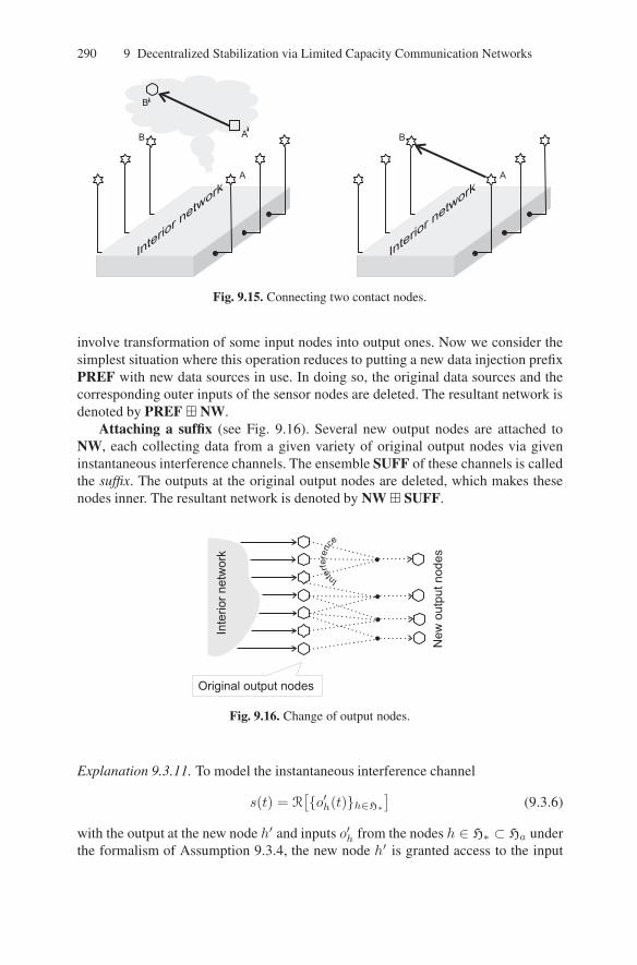
290 9 Decentralized Stabilization via Limited Capacity Communication Networks
Fig. 9.15. Connecting two contact nodes.
involve transformation of some input nodes into output ones. Now we consider thesimplest situation where this operation reduces to putting a new data injection prefixPREF with new data sources in use. In doing so, the original data sources and thecorresponding outer inputs of the sensor nodes are deleted. The resultant network isdenoted by PREF ⊞ NW.
Attaching a suffix (see Fig. 9.16). Several new output nodes are attached toNW, each collecting data from a given variety of original output nodes via giveninstantaneous interference channels. The ensemble SUFF of these channels is calledthe suffix. The outputs at the original output nodes are deleted, which makes thesenodes inner. The resultant network is denoted by NW ⊞ SUFF.
Fig. 9.16. Change of output nodes.
Explanation 9.3.11. To model the instantaneous interference channel
s(t) = R[o′h(t)h∈H∗
](9.3.6)
with the output at the new node h′ and inputs o′h from the nodes h ∈ H∗ ⊂ Ha underthe formalism of Assumption 9.3.4, the new node h′ is granted access to the input

9.4 Decentralized Networked Stabilization: The Problem Statement and Main Result 291
data of all nodes h ∈ H∗. The memory of h′ is structured mh′ =[mhh∈H∗ ,mh′
]
to include the counterparts of the memory contents of all nodes h ∈ H∗. For h′, theadmissible data processing algorithms are confined to those that first process datarelated to a given h ∈ H∗, independently of all other accessible data, to generate asignal o′h(t) and update mh(t) and then produce the node output uh′(t) and updatemh′(t) in such a way that the use of the data associated with the nodes h ∈ H∗ isrestricted to the use of the quantity (9.3.6).4
9.4 Decentralized Networked Stabilization with CommunicationConstraints: The Problem Statement and Main Result
This section offers the formulation of the main problem and results of this chapter.
9.4.1 Statement of the Stabilization Problem
The main problem addressed in this chapter is as follows. We consider lineardiscrete-time multiple sensor and actuator systems of the form:
x(t+ 1) = Ax(t) +l∑
i=1
Biui(t) + ξ(t), x(0) = x0; (9.4.1)
yj(t) = Cjx(t) + χj(t), j = 1, . . . , k. (9.4.2)
Here l and k are the numbers of the actuators and sensors, respectively, and thevariables are as follows:
• x ∈ Rdim(x) – the state,• ui ∈ Rdim(ui) – the output of the ith actuator,• yj ∈ Rdim(yj) – the output of the jth sensor,• ξ(t) ∈ Rdim(x) – the exogenous disturbance,• χj(t) ∈ Rdim(yj) – the noise in the jth sensor.
The system is unstable: There is an eigenvalue λ of the matrix A with |λ| ≥ 1. Theobjective is to stabilize the plant.
This should be accomplished by means of multiple decentralized controllers.Along with sensors and actuators, they are spatially distributed and linked via a givencommunication network. The algorithms of data processing at controllers, sensors,and actuators are to be designed so that the closed-loop system is stable.5
4At first sight, one more requirement is that the node h′ should produce the memorycontent mh identical to that generated at the node h. In fact, this requirement is superfluous.It can be always ensured by reorganizing the memory and data processing at h and h′ so thatboth h and h′ acquire two copies of mh processed in accordance with the algorithms originallyimplemented at h and h′, respectively.
5In this chapter, the term “actuator” denotes a device that is able not only to apply a givencontrol to the plant but also to generate controls. So it may be more correct to call these devices“controllers directly acting upon the plant.”

292 9 Decentralized Stabilization via Limited Capacity Communication Networks
Formally, we suppose that a network NW with unconstrained contact nodes6
is given. Its input and output nodes are associated with the sensors and actuators,respectively (see Fig. 9.17a). The jth sensor acts as the data source for the associatedinput node whose current outer input is thus equal to yj(t). Similarly, the controlui(t) is the current outer output generated by the corresponding output node. Werecall that the algorithm of data processing within the network is denoted by theparameter A in (9.3.2). This parameter should be chosen from the given set A ofadmissible algorithms so that the closed-loop system is stable. The algorithm A willbe also called the (decentralized) control strategy.
Fig. 9.17(a). Decentralized control. Fig. 9.17(b). Control-based extension.
Remark 9.4.1. It follows that in (9.3.2) (on p. 283), the compound vectors of thenetwork inputs and outputs, respectively, are given by
Y (t) = col [y1(t), . . . , yk(t)] , U(t) = col [u1(t), . . . , ul(t)] .
The control strategy A, sequences of noises ξ(t), χj(t), and initial state x0 from(9.4.1) uniquely determine a process in the closed-loop system.
We consider bounded noises and initial states x0:
‖ξ(t)‖ ≤ D <∞, ‖χj(t)‖ ≤ Dyj <∞ ∀t, j, ‖x0‖ ≤ Dx <∞, (9.4.3)
where D,Dyj , Dx > 0, and accept that a control strategy succeeds if it keeps the
stabilization error bounded:
supt
supξ(θ),χj(θ) , x0
‖x(t)‖ <∞. (9.4.4)
Here the second sup is over noises and initial states satisfying (9.4.3).
6See Definition 9.3.8 (on p. 288).

9.4 Decentralized Networked Stabilization: The Problem Statement and Main Result 293
Definition 9.4.2. A decentralized control strategy ensuring (9.4.4) is said to stabilizethe system. If in addition (9.4.4) holds for any iwith ui(t) substituted in place of x(t),the strategy is said to regularly stabilize the system.
Remark 9.4.3. We recall that arbitrary restrictions on the admissible algorithms forthe controllers can be imposed within this problem statement. What is called the“network” captures not only the available ways to transmit information but also therestrictions on the possible ways of data processing by the controllers.
Which networks fit to stabilize a given unstable linear plant under a proper de-sign of the control strategy?
The main result of the chapter is that this question is reducible to the followingstandard question studied in the traditional information sciences.
How much data may be communicated from the input to output nodes across thenetwork that results from a certain extension of the original one?
All limitations on not only communication but also the data processing algorithmsare inherited by the extended network. So the second question concerns communica-tion under the restrictions imposed in the original network.
Remark 9.4.4. The extended network is an artificial and auxiliary object serving theanswer to the primal question.
In the next four subsections, this network is introduced via three steps.
9.4.2 Control-Based Extension of the Network
As was shown in Subsect. 7.8.1 (on p. 233), there is a way to communicate as muchinformation as desired via the plant. In this way, the information can be transmittedfrom any actuator to any sensor that is able to detect the actions of this actuator. Tothis end, the actuator should encode a message by producing a control that impartsto the system motion a certain specific feature. The sensor receives the message byobserving the motion and detecting this feature.
The above phenomenon can be interpreted as if the plant hides several external7
communication channels. The first step to extend the network is explicit incorpora-tion of all these channels into it (see Fig. 9.17b). After this, the resultant network willbe considered in the open loop (out of connection with the plant).
Now we come to details. To start with, we introduce the subspaces of states thatare controllable and nonobservable by the ith actuator and jth sensor, respectively:
L+ci := Lin
[n−1⋃
ν=0
Im (AνBi)
], L−oj :=
n−1⋂
ν=0
x : CjAνx = 0 , (9.4.5)
where n := dim(x). The set of actuator–sensor pairs communicating via the plant is
7With respect to the network given in the problem statement.

294 9 Decentralized Stabilization via Limited Capacity Communication Networks
CVP :=(i, j) : L+c
i 6⊂ L−oj. (9.4.6)
Since control ui influences yj with the delay
di→j := mind = 0, 1, . . . : CjAdBi 6= 0+ 1, (9.4.7)
data transmitted from the ith actuator to the jth sensor incur the same delay.Now let us run over all pairs (i, j) from (9.4.6). For every pair, let us connect
the network contact node associated with the ith actuator with that associated withthe jth sensor. The connection is by means of di→j -delayed channel Ri→j calledthe feedback tunnel (i.e., hidden channel) with the infinite alphabet of the maximalpossible cardinality 2ℵ0 .
Insertion of all these tunnels gives rise to a new network called the control-basedextension CBE(NW) of the original one.
Remark 9.4.5. The input and output nodes of CBE(NW) are identical to those of theoriginal network.
9.4.3 Assumptions about the Plant
To proceed, we need some assumptions about the plant. They in fact come to astrengthened form of Assumption 3.4.24 (on p. 49) with respect to the sensors, andadopting its dual counterpart with respect to the actuators. The reason for imposingAssumption 3.4.24 was discussed in Sect. 3.9 (starting on p. 90). Its strengthening ismotivated by the wish to simplify the design of the stabilizing strategy by avoidingthe technically demanding sequential stabilization approach (see p. 64).
We first state the assumption about the plant in a preliminary form, which is easyto comprehend. Then we give its basic formulation, which is more complicated. Thereader interested in rather ideas than generality may confine himself to the first form.
Assumption 9.4.6.∗ (Restricted form.) The unstable |λ| ≥ 1 eigenvalues λ ofA aredistinct.
Assumption 9.4.6. The unstable subspace Munst(A) of A can be decomposed intothe direct sum Munst(A) =
⊕gν=1Mν of A-invariant (real) subspaces Mν such that
the following two claims hold:
i) For any ν, the spectrum of A|Mν consists of only either one real eigenvalue λ[ν]
or a couple of conjugate complex ones λ[ν] = λ[ν];ii) The subspace Mν is in simple relations with the sensors and actuators: Every
subspace of the form L = L+ci ∩Munst(A) or L−oj ∩Munst(A) is a direct sum of
several subspaces of the form Mν .
We recall that the direct sum of the empty group of subspaces is defined to be 0.Observation 9.4.7. Assumption 9.4.6∗ clearly implies 9.4.6, with Mν being the realinvariant subspaces related to unstable eigenvalues.

9.4 Decentralized Networked Stabilization: The Problem Statement and Main Result 295
Due to Assumption 9.4.6, a proper linear change of the variables shapes x into
x = col(x−s, . . . , x0︸ ︷︷ ︸∼Mst(A)
, x1, . . . , xg1︸ ︷︷ ︸∼M1
, . . .︸︷︷︸∼M2
, . . .︸︷︷︸∼M3
, . . . , . . . xn+︸ ︷︷ ︸∼Mg
), (9.4.8)
where n+ := dimMunst(A). In other words, Mst(A) is the set of all x with xα =0 ∀α ≥ 1, and Mν is the set of all x with zeros at all positions outside a certaingroup of coordinates. With a slight abuse of terminology, xα with α ≥ 1 will becalled unstable modes.
Remark 9.4.8. Any unstable mode xα is related to a unique subspace Mν , whereν = ν(α). So by i), it is associated with an eigenvalueλα := λ[ν(α)]. This associationis unique up to the conjugation in the case of the complex eigenvalue; the modulus|λα| is determined uniquely.
Remark 9.4.9. Given an unstable mode xα and a sensor, this mode is either observedor ignored by this sensor. Similarly, a given actuator either controls the mode or doesnot affect it at all.
More specifically, the claim ii) implies that for any sensor j, the nondetectablesubspace L−oj ∩ Munst(A) is the set of all x with zero coordinates at all positionsoutside a certain groupAj with elements α ≥ 1. Any unstable mode xα with α ∈ Ajdoes not affect the outputs of this sensor. Conversely, it can be restored from theseoutputs (the sensor observes the mode xα) if α 6∈ Aj . Similarly, the stabilizablesubspace L+c
i ∩Munst(A) of any actuator i is the set of all x with zero coordinatesat all positions outside a certain group A[i] with elements α ≥ 1 thanks to ii). Anyunstable mode xα with α 6∈ A[i] is not affected by this actuator. Conversely, thismode is controlled by this actuator if α ∈ A[i].
Remark 9.4.10. Assumption 9.4.6 is true whenever the system is detectable by eachsensor and stabilizable by every actuator.
Indeed, then ii) holds for the decomposition of Munst(A) into the real invariant sub-spaces related to the unstable eigenvalues.
9.4.4 Mode-Wise Prefix
The next step to the new network is a change of the scheme of data injection intoCBE(NW). We introduce new data sources, each associated with a particular unsta-ble mode xα. The data related to mode xα are instantaneously delivered to all sensorsj that observe this mode, i.e., those from the set
Jmw←α :=j = 1, . . . , k : Mν(α) ∩ L−oj = 0
. (9.4.9)
The mode-wise prefix PREFmw is the described scheme of data injection (seeFig. 9.18a).

296 9 Decentralized Stabilization via Limited Capacity Communication Networks
Fig. 9.18(a). Mode-wise prefix. Fig. 9.18(b). Mode-wise suffix.
9.4.5 Mode-Wise Suffix and the Final Extended Network
This suffix displays similar dual relations between the actuators and unstable modes,and it is used to change the output nodes of the network. The new output nodes arealso associated with unstable modes and attached to CBE(NW) via related interfer-ence channels (see Fig. 9.16 on p. 290). The channel related to xα collects data fromall actuators i that control this mode, i.e., those from the set
Imw→α := i : Mν(α) ⊂ L+ci
. (9.4.10)
This channel is instantaneous and additive with the real alphabet R. The mode-wisesuffix is the ensemble SUFFmw of all these additive real channels (see Fig. 9.18b).The mode-wise suffix with quantization SUFFq
mw results from restriction the admis-sible algorithms at any terminal node (associated with an unstable mode) to thoseforming the current outer output as the projection of the currently transmitted realsignal s into the nearest integer.8
Explanation 9.4.11. The locations of the source and the output node associated witha common unstable mode are regarded as different.
This is motivated by the double role of every unstable mode: It is an object of obser-vation on the one hand and control on the other hand.
Explanation 9.4.12. The additive channel is chosen since the cumulative effect of theactuators on the plant (9.4.1) results from summation of the effects caused by eachactuator.
The final extended network that will be of interest further results from attachingboth the mode-wise prefix and mode-wise suffix with quantization
PREFmw ⊞ CBE(NW) ⊞ SUFFqmw (9.4.11)
to the control-based extension CBE(NW) of the original network NW (see Fig. 9.19).
8In the case of uncertainty (v − 1/2 is an integer), the void output ⊛ is produced.

9.4 Decentralized Networked Stabilization: The Problem Statement and Main Result 297
Fig. 9.19. Extended network.
Remark 9.4.13. The network (9.4.11) is disconnected with the plant.
Remark 9.4.14. Due to (9.4.6), (9.4.9), and (9.4.10), any pair (actuator node i)-(sensor node j) affecting and observing, respectively, at least one common unstablemode xα is linked by a feedback tunnel:
CVP ⊃ (i, j) : ∃α = 1, . . . , n+ such that i ∈ Imw→α and j ∈ Jmw←α . (9.4.12)
9.4.6 Network Capacity Domain
As was remarked on p. 293, criterion for stabilizability involves an answer to thequestion: How much data can be communicated across the network (9.4.11)? Specif-ically, data from the informant associated with the unstable mode xα should be sentto the output node related to the same mode.9 The answers to such questions are tra-ditionally given in terms of a fundamental concept of the classic information theory:The capacity (rate) domain.
Now we recall this notion for the particular situation at hand. Its critical feature isthat the network data sources σα and output nodes outα are marked by the commonindex α ∈ [1 : n+]. The sources produce messages yα independently. For any α,the message yα should be transmitted to the equally enumerated node outα, where itappears in the form of the outer output uα of this node. The transmission is arrangedby choosing an admissible algorithm A ∈ A of data processing within the network.
Definition 9.4.15. A networked block code with block length N is an admissibledata processing algorithm A that acts only during the time interval [0 : N − 1],serves sources producing constant message sequences yα(t) ≡ yα ∈ [1 : Fα] ∀t,
9The data streams related to various α should go through the network simultaneously.
298 9 Decentralized Stabilization via Limited Capacity Communication Networks
and generates the outputs in the matching form uα(t) ∈ [1 : Fα] ∪ ⊛.10 The ratevector of this code is defined to be
rcode := col(
log2 F1
N, . . . ,
log2 Fn+
N
). (9.4.13)
Definition 9.4.16. A networked block code is errorless if at the terminal time it cor-rectly recognizes the messages from all sources uα(N − 1) = yα ∀α irrespective ofwhich messages yα ∈ [1 : Fα] were dispatched.
Definition 9.4.17. A vector r ∈ Rn+
is called the achievable rate vector if for ar-bitrarily large N and small ǫ > 0, an errorless networked block code with blocklength N ≥ N exists whose rate vector (9.4.13) approaches r with accuracy ǫ; i.e.,‖rcode − r‖ < ǫ. The capacity domain CD is the set of all achievable rate vectors.
Finding such a domain is a long-standing standard problem in the informationtheory. We refer the reader to [49, 214] for an excellent overview of achievementsand troubles in its solution.
Remark 9.4.18. To underscore the capacity domain of which network is considered,the notation (in brackets) of the network may be added to CD from the right.
Remark 9.4.19. Since the suffix SUFFqmw with quantization admits a smaller range
of data processing algorithms than SUFFmw, the following inclusion holds:
CD (PREFmw ⊞ CBE(NW) ⊞ SUFFqmw)
⊂ CD (PREFmw ⊞ CBE(NW) ⊞ SUFFmw) . (9.4.14)
In some cases, these domains are equal. One of them will be discussed in Re-mark 9.5.20 (on p. 323).
9.4.7 Final Assumptions about the Network
In addition to Assumption 9.3.4 (on p. 285), we need more assumptions about theprimal network NW involved in the stabilization problem setup. They basically meanthat the network is stationary and can be reset to the initial state.
Assumption 9.4.20. For any admissible data processing strategy A ∈ A and timeinstant T = 0, 1, . . ., another admissible strategy Ares ∈ A exists such that thefollowing properties hold:
i) These strategies are identical until t = T ; i.e.,
F(·,A, t) ≡ F(·,Ares, t) for all t = 0, . . . , T and F := O,U,M
and M0(A) = M0(Ares), where O(·),U(·),M(·), and M0(·) are the functionsfrom (9.3.2) (on p. 283);
10The output ⊛ means “no decision.”

9.4 Decentralized Networked Stabilization: The Problem Statement and Main Result 299
ii) The strategy Ares ∈ A resets the network to the initial state at a time T∗ > T :
N(T∗) = N0, I(T∗) = I0, M (T∗) = M0(A)
and can be chosen so that T∗ − T ≤ δTmax, where the constant δTmax does notdepend on A. Moreover, the memory content M can be driven to the state M0(A1)initial for any other a priori chosen strategy A1 ∈ A provided that it is equivalent toA modulo a given finite partition (i.e., ∃ν : A1,A ∈ Mν ) of the memory alphabetM = M = M1 ∪ . . . ∪MQ.
Explanation 9.4.21. It is tacitly assumed that ii) should be true irrespective of theouter inputs of the network. Typically, this means that the strategy Ares ignores theinputs on the interval [T + 1 : T∗].
Assumption 9.4.22. For any two admissible data processing strategies Ai ∈ A, i =1, 2 and time instant T = 0, 1, . . . such that the network driven by the strategy A1
arrives at time T at the state initial for A2
N(T ) = N 0, I(T ) = I0, M(T ) = M0(A2),
another admissible strategy A ∈ A exists that is identical to A1 and A2 on the timeinterval [0 : T − 1] and afterward, respectively: M0(A) = M0(A1) and
F(·,A, t) ≡
F(·,A1, t) for all t = 0, . . . , T − 1
F(·,A2, t− T ) for all t ≥ T , where F := O,U,M.
Explanation 9.4.23. With respect to the data processing algorithms hosted by thecontact nodes, these properties are partly ensured by Assumption 9.3.4 (on p. 285).
To state the last assumption, we start with a technical definition.
Definition 9.4.24. The data processing strategy A ∈ A is said to be τ -periodic(τ = 1, 2, . . .) if in (9.3.2), the functions O(·,A, t),U(·,A, t), and M(·,A, t) areτ -periodic in time: F(·,A, t+ τ) ≡ F(·,A, t+ τ) for all t and F := O,U,M.
The last assumption means that any data processing strategy that drives the networkinto the initial state at some time instant τ can be extended from the interval [0 : τ−1]on [0 :∞) as a τ -periodic strategy.
Explanation 9.4.25. The possibility of τ -periodic extension on any finite interval ofthe form [0 : rτ ], r = 1, 2, . . . follows from Assumption 9.4.22.
Assumption 9.4.26. For any admissible data processing strategy A ∈ A and timeinstant τ = 1, 2, . . . such that the network is in the initial state N(τ) = N0, I(τ) =I0,M(τ) = M0(A) at time τ , a τ -periodic admissible data processing strategyAper ∈ A exists that is identical to A on the time interval [0 : τ − 1].

300 9 Decentralized Stabilization via Limited Capacity Communication Networks
9.4.8 Criterion for Stabilizability
This criterion concerns the stabilization problem posed in Subsect. 9.4.1. We recallthat intS is the interior of the set S.
Theorem 9.4.27. Suppose that Assumptions 9.3.4 (on p. 285), 9.4.6 (on p. 294),9.4.20, 9.4.22, and 9.4.26 hold. We consider the representation (9.4.8) of the statevector and associate any unstable mode xα, α ≥ 1 from (9.4.8) with an unstableeigenvalue λα in accordance with Remark 9.4.8. We also introduce the vector
Λ := col(
log2 |λ1|, . . . , log2 |λn+ |). (9.4.15)
Then the following implications are true:
a) Λ ∈ int CD[PREFmw ⊞ CBE(NW) ⊞ SUFFq
mw
].
⇓b) The network NW hosts a time-periodic admissible control strategy
that regularly stabilizes11the plant.
⇓c) The network NW hosts an admissible control strategy that stabilizes the plant.
⇓d) Λ ∈ CD
[PREFmw ⊞ CBE(NW) ⊞ SUFFq
mw
].
The proof of this theorem will be given in Sects. 9.6 and 9.7. A stabilizing controlstrategy is described in Sect. 9.7.
The implication b) ⇒ c) is evident. It is mentioned to stress that the claims b)and c) are included in a chain of implications with approximately identical extremeterms. So all claims from this chain are “almost equivalent.”
The necessity part of Theorem 9.4.27 can also be slightly improved in the casewhere the vector (9.4.15) contains zero entries: |λα| = 1 for some α.
Remark 9.4.28. If claim c) holds, the concerned capacity domain contains a vectorwith nonzero entries.
The proof of this minor remark will be given in Subsect. 9.8.4 (starting on p. 362).
Corollary 9.4.29. Whenever c) holds, the plant is detectable and stabilizable by theentire set of sensors and actuators, respectively.
Indeed otherwise, there would be an unstable mode xα such that the correspond-ing either data source or output node of PREFmw ⊞ CBE(NW) ⊞ SUFFq
mw is notlinked with the interior network CBE(NW). Then it is impossible to transmit in-formation between these nodes, and so rα = 0 for any achievable rate vector, inviolation of Remark 9.4.28.
11See Definition 9.4.2 (on p. 293).
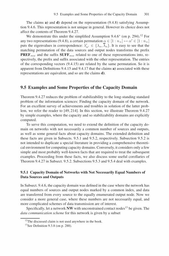
9.5 Examples and Some Properties of the Capacity Domain 301
The claims a) and d) depend on the representation (9.4.8) satisfying Assump-tion 9.4.6. This representation is not unique in general. However its choice does notaffect the contents of Theorem 9.4.27.
We demonstrate this under the simplified Assumption 9.4.6∗ (on p. 294).12 Forany two representations (9.4.8), a certain permutation α ∈ [1 : n+] 7→ α′ ∈ [1 : n+]puts the eigenvalues in correspondence: λ′α′ ∈ λα, λα. It is easy to see that thematching permutation of the data sources and output nodes transforms the prefixPREFmw and the suffix SUFFmw related to one of these representations into, re-spectively, the prefix and suffix associated with the other representation. The entriesof the corresponding vectors (9.4.15) are related by the same permutation. So it isapparent from Definitions 9.4.15 and 9.4.17 that the claims a) associated with theserepresentations are equivalent, and so are the claims d).
9.5 Examples and Some Properties of the Capacity Domain
Theorem 9.4.27 reduces the problem of stabilizability to the long-standing standardproblem of the information sciences: Finding the capacity domain of the network.For an excellent survey of achievements and troubles in solution of the latter prob-lem, we refer the reader to [49, 214]. In this section, we illustrate Theorem 9.4.27by simple examples, where the capacity and so stabilizability domains are explicitlycomputed.
To serve this computation, we need to extend the definition of the capacity do-main on networks with not necessarily a common number of sources and outputs,as well as some general facts about capacity domains. The extended definition andthese facts are given in Subsects. 9.5.1 and 9.5.2, respectively. Subsection 9.5.2 isnot intended to duplicate a special literature in providing a comprehensive theoreti-cal environment for computing capacity domains. Conversely, it considers only a fewsimple and most probably well-known facts that are required to treat the subsequentexamples. Proceeding from these facts, we also discuss some useful corollaries ofTheorem 9.4.27 in Subsect. 9.5.2. Subsections 9.5.3 and 9.5.4 deal with examples.
9.5.1 Capacity Domain of Networks with Not Necessarily Equal Numbers ofData Sources and Outputs
In Subsect. 9.4.6, the capacity domain was defined in the case where the network hasequal numbers of sources and output nodes marked by a common index, and dataare transferred from every source to the equally enumerated output node. Now weconsider a more general case, where these numbers are not necessarily equal, andmore complicated schemes of data transmission are of interest.
Specifically, let a network NW with unconstrained contact nodes13 be given. Thedata communication scheme for this network is given by a subset
12The discussed claim is not used anywhere in the book.13See Definition 9.3.8 (on p. 288).

302 9 Decentralized Stabilization via Limited Capacity Communication Networks
T ⊂ S× Ha, (9.5.16)
where S and Ha are the sets of data sources output nodes, respectively. The set T
lists the pairs that need communication (see Fig. 9.20a). In other words, data shouldbe transmitted from every source σ to all output nodes
out ∈ T←[σ] :=
out : T := (σ, out) ∈ T
=
out1σ, . . . , outsσσ
. (9.5.17)
Fig. 9.20(a). Scheme of communicationacross the network.
Fig. 9.20(b). The simplest scheme.
Explanation 9.5.1. • If T←[σ] = ∅, there are no data to be sent from σ.• Respective independent messages µ1
σ, . . . , µsσσ should be sent from σ to the out-
put nodes listed in (9.5.17).• Any output node outiσ from (9.5.17) should decode and receive only its own
message µiσ from σ: All other messages µjσ, j 6= i are of no interest for outiσ.• In total, any output node out should receive messages from the sources
σ ∈ T→[out] :=σ : (σ, out) ∈ T
. (9.5.18)
• If T→[out] = ∅, the node out should receive nothing.
Remark 9.5.2. The entire ensemble of transmitted messages can be enumeratedµTT∈T
by the elements of the set (9.5.16).
How much data can be transmitted across the network in accordance with a givencommunication scheme, provided that the data streams related to various communi-cating pairs go through the network in parallel? The answer concerns transmittingensembles M =
µTT∈T
of messages of the form µT ∈ [1 : FT ]. Associated withsuch an ensemble is a constant time sequence of messages from any source σ:
yσ(t) ≡ yσ :=
µ(σ,out)
out∈T←[σ]
if T←[σ] 6= ∅⊛ otherwise
.
The transmission is arranged by choosing an admissible algorithm A ∈ A of dataprocessing within the network.

9.5 Examples and Some Properties of the Capacity Domain 303
Definition 9.5.3. A networked block code with block lengthN serving the communi-cation scheme (9.5.16) is an admissible data processing algorithm A that acts onlyduring the time interval [0 : N − 1], deals with input data produced in the aboveway, and generates the outputs in the matching form
uout(t) =
µ′(σ,out)(t)
σ∈T→[out]
, µ′T (t) ∈ [1 : FT ] ∪ ⊛ if T→[out] 6= ∅⊛ otherwise
.
The rate ensemble of this code is defined to be
rcode :=
log2 FTN
T∈T
. (9.5.19)
Definition 9.5.4. A networked block code is errorless if at the terminal time it cor-rectly recognizes the messages for all communicating pairs: µT = µ′T (N−1) ∀T ∈T, irrespective of which messages µT ∈ [1 : FT ] were dispatched.
Definition 9.5.5. An ensemble r =rT ≥ 0
T∈T
is called the achievable rate en-
semble if for arbitrarily largeN and small ǫ > 0, an errorless networked block codewith block length N ≥ N exists whose rate ensemble (9.5.19) approaches r withaccuracy ǫ; i.e., the matching entries differ at most by ǫ. The set of all achievablerate vectors is called the capacity domain for the communication scheme (9.5.16)and denoted by CD[NWT].
In Subsect. 9.4.6, considered was the case where the numbers of sources andoutput nodes are equal, they are enumerated by a common index α, and the commu-nication scheme dictates to transmit data from every source to the equally enumer-ated node (see Fig. 9.20b). Then the pairs from T can be evidently enumerated by thesame indexα, and the definitions from this section come to those from Subsect. 9.4.6.
Conversely, the situation and definitions from this subsection can be reducedto those from Subsect. 9.4.6 up to minor formalities by enumerating the pairs fromT = Tα and attaching a special prefix and suffix to the network NW. The channelsfrom these prefix and suffix are enumerated by the same index and are instantaneousperfect channels with the alphabets of the maximal possible cardinalities coming toand departing from the first and second entries of the pair Tα from and to the sourceand output node associated with α, respectively.
We close the subsection with useful technical facts about the capacity domain.
Lemma 9.5.6. Suppose that a network NW with unconstrained contact nodes14 sat-isfies Assumptions 9.4.20 and 9.4.22 (on p. 298), and a data communication scheme(9.5.16) is given. Then the following claims are true:
(i) The capacity domain CD[NWT] is a closed set, which along with any ele-ment r, contains all elements 0 ≤ r′ ≤ r, where the inequalities are meantcomponent-wise;
14See Definition 9.3.8 (on p. 288).

304 9 Decentralized Stabilization via Limited Capacity Communication Networks
(ii) Whenever there exists an errorless block code whose rate ensemble has nonzeroentries at the positions from some subset T∗ ⊂ T, the capacity domain containsan achievable rate ensemble with nonzero entries at the same positions;
(iii) Let ε > 0 be given. Any r ∈ CD[NWT] can be approximated with accuracyε by the rate ensembles (9.5.19) of errorless networked block codes Am,m =1, 2, . . . of arbitrarily large block lengths N(m)
m→∞−−−−→ ∞ starting at a com-mon initial state: In (9.3.2) (on p. 283), M0(Am′) = M0(Am′′) ∀m′,m′′.
The proof of this lemma is given in Subsect. 9.8.1 (starting on p. 358). The argu-ments of the proof of (iii) also justify the following claim.
Remark 9.5.7. Statement (iii) holds for the capacity domain concerned in Theo-rem 9.4.27.
9.5.2 Estimates of the Capacity Domain from Theorem 9.4.27 and RelevantFacts
This domain is that of the network (9.4.11) (on p. 296), which results from attachingthe mode-wise prefix and suffix to the control-based extension of the primal networkNW. This suffix is composed by interference channels, which are not easy to dealwith when computing the capacity domain. In this subsection, we give simple esti-mates of the above domain by domains related to networks with no new interferencechannels except for those that may be hidden in the original network NW.
The lower estimate to follow concerns the network
PREFmw ⊞ CBE(NW) (9.5.20)
(see Fig. 9.21 on p. 305) whose sources and output nodes are associated with the un-stable modes and actuators, respectively. It is supplied with the transmission scheme
Tmw :=(α, i) : i ∈ Imw→α
(9.5.21)
according to which data from every source ∼ xα should be transmitted to all actua-tors i controlling the corresponding mode xα.
The upper estimate deals with the network PREFmw ⊞ CBE(NW) ⊞ SUFF+mw.
Here the suffix SUFF+mw is obtained from the mode-wise one SUFFmw (see Sub-
sect. 9.4.5) by replacing every additive channel in SUFFmw by several indepen-dent instantaneous channels with the alphabets of the maximal possible cardinalities.These channels connect the input nodes i ∈ Imw→α of the former additive channel withits output node ∼ xα. After this replacement, data going from these input nodes donot incur interference and so arrive at the output node uncorrupted and in full.
In the remainder of this subsection, the assumptions of Theorem 9.4.27 are as-sumed to hold.
Lemma 9.5.8. The following inclusions are true:

9.5 Examples and Some Properties of the Capacity Domain 305
Fig. 9.21. PREFmw ⊞ CBE(NW).
rαn
+
α=1 : rα =∑
i∈Imw→α
rα,i for some
r = rα,i(α,i)∈Tmw ∈ CD[PREFmw ⊞ CBE(NW)Tmw
]
⊂ CD[PREFmw ⊞ CBE(NW) ⊞ SUFFq
mw
]
⊂ CD[PREFmw ⊞ CBE(NW) ⊞ SUFF+
mw
]. (9.5.22)
The proof of this lemma is given in Subsect. 9.8.2 (starting on p. 360).
Corollary 9.5.9. Suppose that different actuators do not influence common unstablemodes Imw→α′ ∩ Imw→α′′ = ∅ ∀α′ 6= α′′. Then SUFF+
mw can be put in place of SUFFqmw
in the statement of Theorem 9.4.27.
This holds since in (9.5.22), the first and third domains are in fact the same under thecircumstances.
Capacity Domain in the Case of Cloned Channels
Now we consider the case where PREFmw and SUFF+mw contain cloned channels.
Specifically, the unstable modes are partitioned into several groups
[1 : n+] = G1 ∪ . . . ∪Gs, Gν′ ∩Gν′′ = ∅ ∀ν′ 6= ν′′ (9.5.23)
such that
Imw→α′ = Imw→α′′ and Jmw←α′ = Jmw←α′′ ∀α′, α′′ ∈ Gν . (9.5.24)
Then the corresponding channels from PREFmw broadcast from the sources ∼ xα′
and ∼ xα′′ , respectively, to a common set of sensor nodes. Similarly, the channelsfrom SUFF+
mw transfer data to the output nodes∼ xα′ and∼ xα′′ , respectively, from

306 9 Decentralized Stabilization via Limited Capacity Communication Networks
a common set of actuator nodes. In this case, the individual data rates rα of communi-cation α 7→ α between the clones α ∈ Gν are obtained by dividing
∑α∈Gν
rα = rνthe data rate rν achievable in the case where in each group of cloned channels, allchannels except for one are discarded (see Fig. 9.22). Now we come to details.
Fig. 9.22(a). Network with cloned channels. Fig. 9.22(b). Reduced network.
Lemma 9.5.10. Let (9.5.23) and (9.5.24) hold.
(i) Consider the prefix PREFmw and suffix SUFF+
mw obtained from PREFmw andSUFF+
mw, respectively, by discarding all channels except for one in every groupGν and marking the remaining source and output node by the index ν. Then
CD[PREFmw ⊞ CBE(NW) ⊞ SUFF+
mw
]=
rαn
+
α=1 : rα ≥ 0;
∑
α∈Gν
rα
s
ν=1
∈ CD[PREFmw ⊞ CBE(NW) ⊞ SUFF
+
mw
]
; (9.5.25)
(ii) Consider the transmission scheme Tmw for the network PREFmw ⊞ CBE(NW)obtained from (9.5.21) by discarding all pairs except for one in every group ofthe form (α, i), α ∈ Gν and marking the remaining pair by the index (ν, i).Then
CD[PREFmw ⊞ CBE(NW)Tmw
]=
rα,i(α,i)∈Tmw : rα,i ≥ 0;
∑
α∈Gν
rα,i
(ν,i)∈Tmw
∈ CD[PREFmw ⊞ CBE(NW)Tmw
].
The proof of this lemma is given in Subsect. 9.8.3 (starting on p. 360).
Aggregated Form of the Stabilizability Criterion
In some cases, the criterion from Theorem 9.4.27 can be rewritten in a more compactform on the basis of Lemma 9.5.10. Specifically, let we be given a decomposition

9.5 Examples and Some Properties of the Capacity Domain 307
Munst(A) =
g⊕
ν=1
Mν (9.5.26)
that satisfies the requirements of Assumption 9.4.6 (on p. 294) except for (i). As-sumption 9.4.6 gives one such decomposition. However there may be other decom-positions with a lesser number of subspaces.
Remark 9.5.11. Suppose that the plant is stabilizable and detectable by any actuatorand sensor, respectively. Then the trivial decomposition Munst(A) = M1 with onlyone subspace can be employed.
The decomposition with the above properties gives rise to a partition (9.5.23)satisfying (9.5.24). Indeed, it is clear that any invariant subspace Mν can be decom-posed into invariant sub-subspaces satisfying (i) from Assumption 9.4.6.15 Then forthe corresponding state mode-wise representation (9.4.8) (on p. 295), every subspaceMν is described as consisting of all vectors such that xα = 0 for all α outside a cer-tain group Gν of unstable modes. Then (9.5.23) and (9.5.24) evidently hold.
In this case,
• PREFmw is composed by the channels associated with the subspaces from(9.5.26) and enumerated by ν = 1, . . . , g. The νth channel broadcasts from thesource∼Mν to all sensors j that observe the subspace: Mν ∩ L−oj = 0.
• SUFF+
mw is composed by g groups of channels associated with the subspacesfrom (9.5.26) and enumerated by ν = 1, . . . , g. The channels of the νth grouparrive at a common output node∼Mν and depart from, respectively, all actuatorsi ∈ I→ν := i : Mν ⊂ L+c
i that control the subspace at hand. These channelsare instantaneous and have the alphabets of the maximal possible cardinalities.
• Tmw consists of all pairs (ν, i) such that the actuator i controls the subspace Mν .
By observing that for the vector r = log2 |λα|n+
α=1 from Theorem 9.4.27,∑
α∈Gν
rα = log2 | detA|Mν |,
we arrive at the following corollary of Lemmas 9.5.8 and 9.5.10.
Corollary 9.5.12. Let a decomposition (9.5.26) satisfying Assumption 9.4.6 with (i)dropped be given. Then the sufficient a) and necessary d) conditions for stabilizabil-ity from Theorem 9.4.27 are ensured by and imply the following claims, respectively:
a′) log2 | detA|Mν | =∑
i∈I→νrν,i ∀ν for some ensemble
rν,i ∈ int CD[PREFmw ⊞ CBE(NW)Tmw
];
d′) The vector
Λred := col(
log2 | detA|M1 |, log2 | detA|M2 |, . . . , log2 | detA|Mg |)
(9.5.27)belongs to CD
[PREFmw ⊞ CBE(NW) ⊞ SUFF
+
mw
].
15Hence, the existence of such a decomposition is equivalent to this assumption.

308 9 Decentralized Stabilization via Limited Capacity Communication Networks
Similarly, we get the following corollary of Lemma 9.5.10 and Corollary 9.5.9.
Corollary 9.5.13. Suppose that different actuators do not influence common unsta-ble modes Imw→α′ ∩ Imw→α′′ = ∅ ∀α′ 6= α′′, and a decomposition (9.5.26) satisfyingAssumption 9.4.6 with (i) dropped is given. Then in Theorem 9.4.27, the followinginclusions a′′) and d′′) can be substituted in place of a) and d), respectively:
a′′) Λred ∈ int CD[PREFmw ⊞ CBE(NW) ⊞ SUFF
+
mw
];
d′′)Λred ∈ CD[PREFmw ⊞ CBE(NW) ⊞ SUFF
+
mw
].
9.5.3 Example 1: Platoon of Independent Agents
The main purpose of this rather special example is to highlight the typical phenomenathat are encountered in networked stabilization and are caused by the possibility ofinformation transmission by means of control.
We consider a platoon of s unstable controllable agents AAi with independentdynamics
xi(t+ 1) = Aixi(t) +Biui(t) + ξi(t), i = 0, . . . , s− 1,
each equipped by a separate controller Ci (with an unlimited memory and computingcapability) and subjected to a bounded exogenous disturbance ξi(t). So the agentscould stabilize their motions about the required trajectories, provided each of themobserves its own state. However, any agent AAi has access to noisy data only aboutthe state of its “cyclic follower” AAi− , i− := i−1( mod s). These data are enoughto detect the state of the follower with a bounded error and are sent to AAi via adigital perfect channel with capacity ci− (see Fig. 9.23a, where s = 4). The agentsdo not communicate with each other. Is it possible to stabilize the platoon motion?
AA
C0
0
C1 AA 1
C2
AA 2
AA 3 3C
c
c
0
2
c1
c3
Fig. 9.23(a). Stabilization of autonomousagents.
Fig. 9.23(b). Control-based extension.
Since none of the agents observes its own state, the answer seems to be in thenegative at first sight. However, the following claim holds.

9.5 Examples and Some Properties of the Capacity Domain 309
Proposition 9.5.14. The platoon is stabiliazible whenever the unstable parts A+i :=
Ai|Munst(Ai) of the matrices Ai satisfy the inequality
log2 | detA+0 |+ · · ·+ log2 | detA+
s−1| < mini=0,...,s−1
ci.
This inequality is necessary for stabilizability, provided that ≤ is put in place of <.
This proposition is underlaid by the fact that data can be transmitted by meansof controls. This possibility is explicitly displayed by the control-based extension ofthe network at hand (see Fig. 9.23b). It follows that data about the ith agent can bedelivered to its controller Ci via the route depicted by dotted arrows in Fig. 9.24.
Fig. 9.24. The information exchange in the system.
Proof of Proposition 9.5.14. It is easy to see that Assumptions 9.3.4, 9.4.6,9.4.20, 9.4.22, and 9.4.26 (on pp. 285, 294, 298, and 299) are satisfied. (The sen-sor and actuator nodes are associated with AAi and Ci, respectively. Initially, thememories of these nodes are empty.) The entire state of the system consists ofthe states of the agents x = col (x0, . . . , xs−1), and its dynamical matrix equalsA = diag(A0, . . . , As−1). By putting Mν := x : xi = 0 ∀ i 6= ν − 1, xν−1 ∈Munst(Aν−1), we clearly get a decomposition (9.5.26) (with g := s) satisfying therequirements of Assumption 9.4.6 (on p. 294) except for (i). Since different actua-tors do not influence common unstable modes, we see that the situation is like inCorollary 9.5.13. By this corollary, it suffices to show that the capacity domain ofthe control-based extension of the network at hand (see Fig. 9.23b) is given byr = ris−1
i=0 : ri ≥ 0 ∀i, r0 + r1 + · · ·+ rs−1 ≤ mini=0,...,s−1
ci. (9.5.28)
Here ri is the rate at which data can be transmitted from AAi to Ci.Sufficiency. If
∑i ri < mini ci and ri ≥ 0, the control-based extension is evi-
dently able to accommodate simultaneously s continuous stationary fluid flows alongthe dotted directed arcs from Fig. 9.24 of respective intensities r0, . . . , rs−1. Then thearguments from the first part of the proof of Theorem 3.1 [69] (based on a proper timedivision multiplexing) show that r is an achievable rate vector. Then Lemma 9.5.6(on p. 303) implies that (9.5.28) is a subset of the capacity domain.

310 9 Decentralized Stabilization via Limited Capacity Communication Networks
Necessity. The above “fluid” consideration is not relevant any longer.16 Let r bean achievable rate vector. By Definition 9.4.17 (on p. 298), for any ε > 0, an errorlessnetworked block code with block lengthN and input alphabets [1 : Fi] = µi existssuch that |ri − N−1 log2 Fi| < ε ∀i. Let Ai and Ci stand for the sequences of allinput signals received by AAi and Ci, respectively, since t = 0 until t = N − 1. Asfollows from Fig. 9.23b,
Ci+ = Ci(Ai), where i+ := i+ 1 mod s, Ai = Ri(Ci, µi) ∀i.
(We recall that capital script letters denote deterministic functions.) Since the codeis errorless, µi = Mi(Ci). Thus Ci+ = Ci
Ri[Ci,Mi(Ci)]
∀i; i.e., Cjs−1
j=0 =
Fi(Ci)∀i and so (µj)s−1j=0 = Pi(Ci) for all i and µi ∈ [1 : Fi]. Since Ci+ is received
over the channel of capacity ci, it follows that∑
j log2 Fj ≤ Nci ∀i. So∑
i ri ≤sε+
∑j N−1 log2 Fj ≤ sε+mini ci. Letting ε→ 0 shows that the vector r belongs
to (9.5.28). ⊓⊔
9.5.4 Example 2: Plant with Two Sensors and Actuators
In this subsection, we consider a particular case of the linear system (9.4.1), (9.4.2)(on p. 291) with two both sensors and actuators (l = k = 2), which are directly linkedby perfect channels with given finite capacities (see Fig. 9.25a, where the sensors andactuators are marked by S1, S2 and A1, A2, respectively). The case where some ofthese channels do not occur is not excluded and identified with the situation wherethe corresponding capacity is zero cji = 0. The plant is assumed to be detectable andstabilizable by the entire sets of the sensors and actuators, respectively.
Actuators with Nonintersecting Zones of Influence
We start with the case where the actuators affect no common unstable mode. As-sumption 9.4.6 (on p. 294) is still supposed to hold. Then the unstable subspace ofthe plant can be decomposed as follows:
Munst(A) = M11 ⊕Mb1 ⊕M21 ⊕M12 ⊕Mb2 ⊕M22, (9.5.29)
where
• Mji, j 6= b is the subspace of states controllable by the ith actuator, observableby the jth sensor, and nonobservable by the companion sensor;
16In [69], the existence of the continuous fluid flows with intensities matching the datarates of a given coding decoding scheme was justified only for the case of one recipient. Thepaper [4] offers extensions on the case where a single informant broadcasts to several recipi-ents over a network and data processing strategies are restricted to the so-called alpha-codes.The authors are unaware of research, where relevant facts concerning the fluid-like treatmentof information streams were justified for the case of several informants and recipients, as isrequired now.

9.5 Examples and Some Properties of the Capacity Domain 311
Fig. 9.25(a). System with two sensors and ac-tuators.
Fig. 9.25(b). Control-based extension.
• Mbi is the subspace of states controllable by the ith actuator and observable byboth sensors.
The topological entropy of the related part of the open-loop system is denoted by
hνi := log2 | detA|Mνi | ν = 1, 2, b, i = 1, 2.
These notations are also explained in Table 9.1.
Controllable byObservable by Actuator 1 Actuator 2Only sensor 1 h11 h12
Both sensors hb1 hb2
Only sensor 2 h21 h22
Table 9.1. Entropies of various parts of the system.
Explanation 9.5.15. It is not excluded that some of the above parts may degenerateMνi = 0. Then hνi := 0.
To state conditions for stabilizability, we introduce the following operations over2× 2-matricesM = (m11 m12
m21 m22):
• [M ]↔ := m11 +m12 — the sum of the elements from the first row;• [M ]↔ := m21 +m22 — the sum of the elements from the second row;• l[M ] := m11 +m21 — the sum of the elements from the first column;• [M ]l := m12 +m22 — the sum of the elements from the second column;
• Σij−(M) :=∑
(i′,j′)6=(i,j) mi′,j′ — the sum of all entries except for (i, j)th one.
We also introduce the following matrices of entropies and capacities:
H :=
(h11 h12
h21 h22
), C :=
(c11 c12c21 c22
).
We start with the situation where the following property holds.

312 9 Decentralized Stabilization via Limited Capacity Communication Networks
Assumption 9.5.16. Any sensor is able to detect the actions of every actuator:L+ci 6⊂ L−oj ∀i, j.
Proposition 9.5.17. Let Assumption 9.5.16 be true. Whenever the plant is stabiliz-able via the network at hand, the following relations hold:
[H ]↔ ≤ [C]
↔, [H ]↔ ≤ [C]↔
l[H + diag(hb1,hb2)] ≤l [C] , [H + diag(hb1,hb2)]l ≤ [C]l
Σij−(H) + hbj′ ≤ Σij−(C) ∀i, j = 1, 2, (9.5.30)
where j′ := 1 if j = 2 and j′ = 2 if j = 1.Conversely, if relations (9.5.30) hold with the strict inequality signs, the plant is
regularly stabilizable.17
Proof of Proposition 9.5.17
By Corollary 9.5.13, the proof is reduced to computation of the capacity domainCD[PREFmw ⊞ CBE(NW) ⊞ SUFF
+
mw
]with respect to the decomposition (9.5.29).
Thanks to Assumption 9.5.16, the control-based extension CBE(NW) looks as de-
picted in Fig. 9.25b. The reduced both prefix PREFmw and suffix SUFF+
mw involvesix sources and output nodes, respectively. The source data and outputs are associ-ated with the subspaces from (9.5.29) and marked by the corresponding indices νi.The components of the rate vectors r are enumerated similarly rνi, and the matrix
R = ( r11 r12r21 r22 ) is associated with r. The network PREFmw ⊞ CBE(NW) ⊞ SUFF+
mwis shown in Fig. 9.26, where for conciseness, the cloned channels from the suffix andprefix are depicted as one channel with compound input or output. Due to Corol-lary 9.5.13, it suffices to show that the capacity domain of this network is describedby the following set of inequalities, which the main part results from (9.5.30) byputting rνi in place of hνi:
[R]↔ ≤ [C]
↔, [R]↔ ≤ [C]↔
l[R+ diag(rb1, rb2)] ≤l [C] , [R+ diag(rb1, rb2)]l ≤ [C]l
Σij−(R) + rbj′ ≤ Σij−(C) ∀i, j = 1, 2, rνi ≥ 0.
In the expanded form, this system looks as follows:
r11 + r12 ≤ c11 + c12, r21 + r22 ≤ c21 + c22;
r11 + r21 + rb1 ≤ c11 + c21, r12 + r22 + rb2 ≤ c12 + c22;
r11 + r12 + r21 + rb1 ≤ c11 + c12 + c21;
r22 + r12 + r21 + rb2 ≤ c22 + c12 + c21;
r11 + r22 + r12 + rb2 ≤ c11 + c22 + c12;
r11 + r22 + r21 + rb1 ≤ c11 + c22 + c21, rνi ≥ 0. (9.5.31)

9.5 Examples and Some Properties of the Capacity Domain 313
Fig. 9.26. PREFmw ⊞ CBE(NW) ⊞ SUFF+mw.
Sufficiency. We are going to show that any vector r satisfying (9.5.31) is anachievable rate vector. Modulo the arguments from the first part of the proof ofTheorem 3.1 [69] (based on a proper time division multiplexing), this goal will beachieved if we show that the network from Fig. 9.26 is able to transmit simultane-ously six continuous stationary fluid flows of respective intensities yνi ∼ rνi, ν =1, 2, b, i = 1, 2. This will be accomplished via two steps. At the first step, we provethis claim assuming that the “central” input flows are discarded: ybi := 0. Thisshapes (9.5.31) into
r11 + r12 ≤ c11 + c12, r21 + r22 ≤ c21 + c22;
r11 + r21 ≤ c11 + c21, r12 + r22 ≤ c12 + c22;
r11 + r12 + r21 ≤ c11 + c12 + c21, r22 + r12 + r21 ≤ c22 + c12 + c21;
r11 + r22 + r12 ≤ c11 + c22 + c12;
r11 + r22 + r21 ≤ c11 + c22 + c21, rij ≥ 0. (9.5.32)
At the second step, we consider the general case of nonzero central flows.Step 1. Consider a matrix R satisfying (9.5.32) and the distribution
rij = r′ij + r′′ij , r′ij ≥ 0, r′′ij ≥ 0 (9.5.33)
of the input flows along the arcs of the network depicted in Fig. 9.27. For example,the flow r11 is divided into two subflows. One of them r′11 goes directly from S1 toA1. The other r′′11 goes first to A2, then to S2 over the feedback tunnel, and ultimatelyfrom S2 to A1. The conditions necessary and sufficient for the network to be able toaccommodate the subflows are as follows:
r′11 + r′′12 + r′′21 ≤ c11, r′22 + r′′12 + r′′21 ≤ c22;r′12 + r′′11 + r′′22 ≤ c12, r′21 + r′′11 + r′′22 ≤ c21. (9.5.34)
17See Definition 9.4.2 (on p. 293).

314 9 Decentralized Stabilization via Limited Capacity Communication Networks
Thus it should be demonstrated that whenever (9.5.32) holds, the quantities rij canbe splitted (9.5.33) into addends satisfying (9.5.34).
Fig. 9.27. Distribution of the flows.
We shall argue by contradiction. Suppose that this claim fails to be true. Then theconvex cone
K := R : rij ≤ cij ∀i, j = 1, 2does not intersect the image P of the set described by (9.5.33) (where rij are givenand satisfy (9.5.32)) under the linear operator
(r′ij , r
′′ij)i,j=1,2
7→ R :=
(r′11 + r′′12 + r′′21 r
′12 + r′′11 + r′′22
r′21 + r′′11 + r′′22 r′22 + r′′12 + r′′21
). (9.5.35)
It follows that the convex coneK and compact convex set P can be strictly separatedby a hyperplane: numbers θij , i, j = 1, 2 exist such that
supR∈K
∑
ij
θijrij < infR∈P
∑
ij
θijrij (9.5.36)
and∑ij |θij | > 0. Since sup is finite, we have θij ≥ 0. Hence
supR∈K
∑
ij
θijrij =∑
ij
θijcij .
To compute inf , we expand R in the form (9.5.35), invoke (9.5.33), and take intoaccount that minr′,r′′≥0:r′+r′′=r θ
′r′+θ′′r′′ = rminθ′, θ′′. It follows that (9.5.36)shapes into
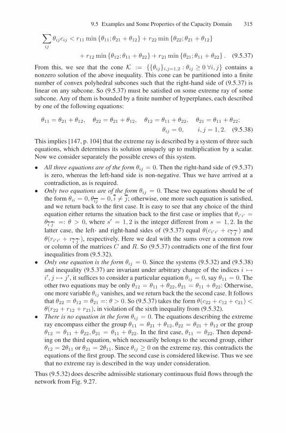
9.5 Examples and Some Properties of the Capacity Domain 315
∑
ij
θijcij < r11 min θ11; θ21 + θ12+ r22 min θ22; θ21 + θ12
+ r12 min θ12; θ11 + θ22+ r21 min θ21; θ11 + θ22 . (9.5.37)
From this, we see that the cone K := θiji,j=1,2 : θij ≥ 0 ∀i, j contains anonzero solution of the above inequality. This cone can be partitioned into a finitenumber of convex polyhedral subcones such that the right-hand side of (9.5.37) islinear on any subcone. So (9.5.37) must be satisfied on some extreme ray of somesubcone. Any of them is bounded by a finite number of hyperplanes, each describedby one of the following equations:
θ11 = θ21 + θ12, θ22 = θ21 + θ12, θ12 = θ11 + θ22, θ21 = θ11 + θ22;
θij = 0, i, j = 1, 2. (9.5.38)
This implies [147, p. 104] that the extreme ray is described by a system of three suchequations, which determines its solution uniquely up to multiplication by a scalar.Now we consider separately the possible crews of this system.
• All three equations are of the form θij = 0. Then the right-hand side of (9.5.37)is zero, whereas the left-hand side is non-negative. Thus we have arrived at acontradiction, as is required.
• Only two equations are of the form θij = 0. These two equations should be ofthe form θii = 0, θij = 0, i 6= j; otherwise, one more such equation is satisfied,and we return back to the first case. It is easy to see that any choice of the thirdequation either returns the situation back to the first case or implies that θi′i′ =θi′j′ =: θ > 0, where s′ = 1, 2 is the integer different from s = 1, 2. In thelatter case, the left- and right-hand sides of (9.5.37) equal θ(ci′i′ + ci′j′) andθ(ri′i′ + ri′j′), respectively. Here we deal with the sums over a common rowor column of the matrices C and R. So (9.5.37) contradicts one of the first fourinequalities from (9.5.32).
• Only one equation is the form θij = 0. Since the systems (9.5.32) and (9.5.38)and inequality (9.5.37) are invariant under arbitrary change of the indices i 7→i′, j 7→ j′, it suffices to consider a particular equation θij = 0, say θ11 = 0. Theother two equations may be only θ12 = θ11 + θ22, θ21 = θ11 + θ22: Otherwise,one more variable θij vanishes, and we return back the the second case. It followsthat θ22 = θ12 = θ21 =: θ > 0. So (9.5.37) takes the form θ(c22 + c12 + c21) <θ(r22 + r12 + r21), in violation of the sixth inequality from (9.5.32).
• There is no equation in the form θij = 0. The equations describing the extremeray encompass either the group θ11 = θ21 + θ12, θ22 = θ21 + θ12 or the groupθ12 = θ11 + θ22, θ21 = θ11 + θ22. In the first case, θ11 = θ22. Then depend-ing on the third equation, which necessarily belongs to the second group, eitherθ12 = 2θ11 or θ21 = 2θ11. Since θij ≥ 0 on the extreme ray, this contradicts theequations of the first group. The second case is considered likewise. Thus we seethat no extreme ray is described in the way under consideration.
Thus (9.5.32) does describe admissible stationary continuous fluid flows through thenetwork from Fig. 9.27.

316 9 Decentralized Stabilization via Limited Capacity Communication Networks
Step 2. Now we revert to the general case, where the central flows are not neces-sarily zero (see Fig. 9.26). The idea is to split these flows
rbi = r′bi + r′′bi, r′bi, r′′bi ≥ 0 (9.5.39)
into subflows r′bi, r′′bi to the nodes S1 and S2, respectively. At these nodes, these sub-
flows are added to the main flows from these nodes to the corresponding recipients:
r11 := r11 + r′b1, r12 := r12 + r′b2, r21 := r21 + r′′b1, r22 := r22 + r′′b2.
By making these substitutions in (9.5.32), we get the conditions under which thestatic flow can be accommodated by the network from Fig. 9.26:
r11 + r12 + r′b1 + r′b2 ≤ c11 + c12, r21 + r22 + r′′b1 + r′′b2 ≤ c21 + c22;
r11 + r21 + rb1 ≤ c11 + c21, r12 + r22 + rb2 ≤ c12 + c22;
r11 + r12 + r21 + rb1 + r′b2 ≤ c11 + c12 + c21;
r22 + r12 + r21 + rb2 + r′′b1 ≤ c22 + c12 + c21;
r11 + r22 + r12 + rb2 + r′b1 ≤ c11 + c22 + c12;
r11 + r22 + r21 + rb1 + r′′b2 ≤ c11 + c22 + c21. (9.5.40)
Thus it should be shown that whenever (9.5.31) holds, the central flows can be de-composed (9.5.39) in such a way that (9.5.40) is true. The conditions imposed by(9.5.39) and the four last relations from (9.5.40) are equivalent to
max
0; r22 + r12 + r21 + rb2 + rb1 − c22 − c12 − c21≤ r′b1
≤ minrb1; c11 + c22 + c12 − r11 − r22 − r12 − rb2
;
max0; r11 + r22 + r21 + rb1 + rb2 − c11 − c22 − c21
≤ r′b2
≤ minrb2; c11 + c12 + c21 − r11 − r12 − r21 − rb1
.
Here in both chains of inequalities, the starting term does not exceed the terminalone due to (9.5.31). So it should be checked that the last system of inequalities has asolution r′b1, r
′b2 common with the first two inequalities from (9.5.40):
r21 + r22 + rb1 + rb2 − c21 − c22 ≤ r′b1 + r′b2 ≤ c11 + c12 − r11 − r12.
This holds if and only if

9.5 Examples and Some Properties of the Capacity Domain 317
max
0; r22 + r12 + r21 + rb2 + rb1 − c22 − c12 − c21
+ max0; r11 + r22 + r21 + rb1 + rb2 − c11 − c22 − c21
≤ c11 + c12 − r11 − r12 and
r21 + r22 + rb1 + rb2 − c21 − c22≤ min
rb1; c11 + c22 + c12 − r11 − r22 − r12 − rb2
+ minrb2; c11 + c12 + c21 − r11 − r12 − r21 − rb1
.
At the same time, it is easy to check that these inequalities follow from (9.5.31). Thiscompletes the proof of the sufficiency part.
Necessity. Let r be an achievable rate vector. By Definition 9.4.17 (on p. 298),for any ε > 0, an errorless networked block code with block length N and inputalphabets [1 : Fνi] (with elements yνi) exists such that
|rνi −N−1 log2 Fνi| < ε ∀ν = 1, 2, b, i = 1, 2.
According to Fig. 9.26, data about p = (y11, y12) are injected into the networkvia the perfect channels S1 7→ A1 and S1 7→ A2 of the total capacity c11 + c12.So if the total number of such pairs exceeds 2N(c11+c12), there are pairs that cannotbe distinguished from the information taken from the network. Hence F11 × F12 ≤2N(c11+c12) and so
r11 + r12 ≤ N−1 [log2 F11 + log2 F12] + 2ε ≤ c11 + c12 + 2ε. (9.5.41)
Letting ε → 0 results in the first inequality from (9.5.31). The second one is estab-lished likewise.
The third inequality is obtained via similar argument with focusing attention onthe node A1, where y11, y21, yb1 are correctly decoded, and noting that all data ac-cessible at this node ultimately arrive via two channels S1 7→ A1 and S2 7→ A1 ofthe total capacity c11 + c21. The fourth inequality is established likewise.
To justify the fifth inequality, we consider data transmission under the assumptiony22 ≡ 1, yb2 ≡ 1. Let Sji stand for the sequence of all messages received over thechannel Sj 7→ Ai since t = 0 until t = N − 1. As follows from Fig. 9.26,
y11 = Y11[S11, S21], y12 = Y12[S12, S22]y21 = Y21[S11, S21]yb1 = Yb1[S11, S21]
, S22 = S22[y21, yb1S11, S12, S21].
(We recall that capital script letters denote deterministic functions.) It follows that
S22 = S22 Y21[S11, S21],Yb1[S11, S21], S11, S12, S21 ,and hence (y11, y12, y21, yb1) is a function of (S11, S12, S21). The first sequenceranges over the set of the size F11×F12×F21×Fb1, whereas the second one belongsto a set of the size≤ 2N(c11+c12+c21). ThusF11×F12×F21×Fb1 ≤ 2N(c11+c12+c21),which results in the fifth inequality from (9.5.31).
The remaining inequalities are established likewise. ⊓⊔

318 9 Decentralized Stabilization via Limited Capacity Communication Networks
Two Independent Agents
Up to this point, it was assumed that any sensor is able to detect the actions of everyactuator. This implies four feedback tunnels in Fig. 9.25b (on p. 311). There also maybe the cases where only three or two such tunnels occur. (One tunnel and no tunnelsare impossible since the unstable plant is detectable and stabilizable by the entire setsof sensors and actuators, respectively.)18 Now we consider the case of two feedbacktunnels, still assuming that the zones of influence of the actuators are disjoint. Bychanging enumeration of the sensors, if necessary, this case can be reduced to thesituation where sensor Si detects the actions of only the matching actuator Ai. Thenthe unstable subspace of the plant can be decomposed as follows:
Munst(A) = M1 ⊕M2, (9.5.42)
where
• Mi is the subspace of states controllable by the ith actuator, observable by theith sensor, and nonobservable by the companion sensor.
The observations are still transmitted via the network from Fig.9.25a.The situation can be interpreted as if there are two independent agents with the
state spaces M1 and M2, respectively, each equipped with its own actuator and sen-sor measuring the state of the owner. At first sight, it may seem that then the crosschannels S1 7→ A2 and S2 7→ A1 are useless, and the conditions for stabilizabilitydisintegrate into
log2 | detA|Mi | ≤ cii, i = 1, 2.
However, the next proposition shows that this is not the case, and the system can bestabilized even if c11 = c22 = 0.
Proposition 9.5.18. Whenever the plant is stabilizable via the network at hand, thefollowing relations hold:
log2 | detA|M1 | ≤ c11+minc12, c21, log2 | detA|M2 | ≤ c22+minc12, c21;log2 | detA|Munst(A)| ≤ c11 + c22 + minc12, c21. (9.5.43)
Conversely, if relations (9.5.43) hold with the strict inequality signs, the plant isregularly stabilizable.19
Proof of Proposition 9.5.18
By Corollary 9.5.13 (on p. 308), the proof is reduced to computation of the capac-
ity domain CD[PREFmw ⊞ CBE(NW) ⊞ SUFF
+
mw
]with respect to the decompo-
sition (9.5.42). The control-based extension CBE(NW) is depicted in Fig. 9.28a.
18It is tacitly assumed that no actuator or sensor is useless for stabilization: L+ci 6⊂
Mst(A), L−oj 6⊃ Munst(A) ∀i, j.
19See Definition 9.4.2 (on p. 293).

9.5 Examples and Some Properties of the Capacity Domain 319
The reduced prefix PREFmw and suffix SUFF+
mw contain two sources and outputnodes, respectively. The data from these sources and outputs at these nodes are as-sociated with the subspaces from (9.5.42) and marked by the corresponding indicesyi. The components of the rate vectors r are enumerated similarly ri. The network
PREFmw ⊞ CBE(NW) ⊞ SUFF+
mw is shown in Fig. 9.28b.
Fig. 9.28(a). Control-based extension. Fig. 9.28(b). The network with the pre-fix and suffix.
Due to Corollary 9.5.13, it suffices to show that the capacity domain of this net-work is described by the following set of inequalities:
r1 ≤ c11 + minc12, c21, r2 ≤ c22 + minc12, c21;r1 + r2 ≤ c11 + c22 + minc12, c21. (9.5.44)
Sufficiency. We are going to show that any vector r satisfying (9.5.44) is an achiev-able rate vector. As before, this is reduced to showing that the network fromFig. 9.28b is able to transmit simultaneously two continuous stationary fluid flows ofrespective intensities yi ∼ ri, i = 1, 2. Consider the distribution
ri = r′i + r′′i , r′i, r′′i ≥ 0 (9.5.45)
of the input flows along the arcs of the network depicted in Fig. 9.29. The conditionsnecessary and sufficient for the network to be able to accommodate the subflows are
r′1 ≤ c11, r′2 ≤ c22, r′′1 + r′′2 ≤ minc12, c21. (9.5.46)
Let us pickr′i := mincii, ri and r′′i := ri − r′i.
Then (9.5.45) and the first two relations from (9.5.46) are true. The third one takesthe form
r1 −minc11, r1+ r2 −minc22, r2= maxr1 − c11, 0+ maxr2 − c22, 0 ≤ minc12, c21

320 9 Decentralized Stabilization via Limited Capacity Communication Networks
Fig. 9.29. Distribution of the flows.
and is immediate from (9.5.44).Necessity. Let r be an achievable rate vector. By Definition 9.4.17 (on p. 298),
for any ε > 0, an errorless networked block code with block length N and inputalphabets [1 : Fi] (with elements yi) exists such that |ri − N−1 log2 Fi| < ε ∀i =1, 2. Let Sji stand for the sequence of all messages received over the channel Sj 7→Ai since t = 0 until t = N − 1. According to Fig. 9.28b,
S11 = S11[y1, S21], S12 = S12[y1, S21],S21 = S21[y2, S12], S22 = S22[y2, S12],
y1 = Y1[S11, S21];y2 = Y2[S12, S22].
Under the assumption y2 ≡ 1,
S12 = S12 [Y1[S11, S21], S21] =: S12[S11, S21], S21 = S21[1, S12] =: S21[S12].
Thus given S11, the sequences S12 and S21 are computable from each other. Theybelong to sets of the sizes 2Nc12 and 2Nc21 , respectively. Hence every of them in factlies in a set of cardinality 2N minc12,c21. It follows that the pair [S11, S21] takes nomore than 2Nc11×2N minc12,c21 values. Since y1 ∈ [1 : F1] is a function of this pair,we arrive at the first relation from (9.5.44) by letting ε→ 0, just like in (9.5.41). Thesecond relation is established likewise by putting y1 ≡ 1 and considering arbitraryy2 ∈ [1 : F2]. The third relation is justified by the same argument applied to arbitraryyi ∈ [1 : Fi], i = 1, 2 by noting that then S12 and S21 are computable from eachother given both S11 and S22. ⊓⊔
Actuators with Identical Zones of Influence
In this case, the plant is stabilizable by any actuator (since the entire set of actuatorsstabilizes it). We still suppose that no sensor is useless for stabilization: L−oj 6⊃Munst(A). The unstable subspace is decomposed as follows:

9.5 Examples and Some Properties of the Capacity Domain 321
Munst(A) = M1 ⊕Mb ⊕M2, (9.5.47)
where
• Mj, j 6= b is the subspace of states observable by the jth sensor and nonobserv-able by the companion sensor;
• Mb is the subspace of states observable by both sensors.
Proposition 9.5.19. Whenever the plant is stabilizable via the network at hand, thefollowing relations hold:
log2 | detA|M1 | ≤ c11 + c12, log2 | detA|M2 | ≤ c21 + c22;
log2 | detA|Munst(A)| ≤ c11 + c22 + c12 + c21. (9.5.48)
Conversely, if relations (9.5.48) hold with the strict inequality signs, the plant isregularly stabilizable.20
Proof of Proposition 9.5.19
Now there are four feedback tunnels, and the control-based extension of the networkis depicted in Fig. 9.25b (on p. 311). We are going to employ Corollary 9.5.12 (onp. 307) related to the decomposition (9.5.47).
Sufficiency. Let (9.5.48) be true with the strict inequality signs. To prove stabiliz-ability, it suffices to show that a′) of Corollary 9.5.12 (on p. 307) holds. In service ofthe data transmission scheme Tmw (see p. 307), the network PREFmw ⊞ CBE(NW)from a′) is depicted in Fig. 9.26 (on p. 313). So the capacity domain CD
[PREFmw ⊞
CBE(NW)Tmw]
is described by (9.5.31). So it suffices to show that the numbersri := log2 | detA|Mi |, rb := log2 | detA|Mb | can be decomposed
ri := ri1 + ri2, ri1, ri2 ≥ 0, i = 1, 2, b (9.5.49)
into addends satisfying (9.5.31) with the strict inequality signs. Note that the initialassumption of this part of the proof means that
r1 ≤ c11 + c12, r2 ≤ c21 + c22, r1 + r2 + rb ≤ c11 + c22 + c12 + c21, (9.5.50)
where all signs are strict. However, it suffices to show that (9.5.50) implies (9.5.31)in the case of nonstrict inequalities. (Then the claim for the strict inequalities followsby a small perturbation of cij’s.)
We decompose r1 and r2 as follows:
r11 := minr1; c11, r12 := max0; r1 − c11;r21 := max0; r2 − c22, r22 := minr2; c22. (9.5.51)
This is a decomposition indeed since
20See Definition 9.4.2 (on p. 293).

322 9 Decentralized Stabilization via Limited Capacity Communication Networks
ri1+ri2 = minri; cii+max0; ri−cii = minri; cii+ri+max−ri;−cii= minri; cii+ ri −minri; cii = ri.
Thanks to (9.5.49), the first two inequalities in (9.5.31) and (9.5.50) are identical. Werewrite the remaining inequalities from (9.5.31) as conditions on rb1 and rb2:
0 ≤ rb1 ≤ minc11 + c21 − r11 − r21;
c11 + c12 + c21 − r11 − r12 − r21;c11 + c22 + c21 − r11 − r22 − r21
;
0 ≤ rb2 ≤ minc12 + c22 − r12 − r22;
c22 + c12 + c21 − r22 − r12 − r21;c11 + c22 + c12 − r11 − r22 − r12
.
Here the expressions on the right are non-negative, since due to (9.5.51),
rii ≤ cii, r12 := max0; r1 − c11(9.5.50)≤ max0; c11 + c12 − c11 = c12;
and r21 ≤ c21 (9.5.52)
by the similar argument. It follows that rb can be decomposed into rb1 and rb2 sothat the remaining inequalities from (9.5.31) are satisfied if and only if
rb ≤ minc11 + c21 − r11 − r21;
c11 + c12 + c21 − r1 − r21;c11 + c22 + c21 − r11 − r2
+ minc12 + c22 − r12 − r22;
c22 + c12 + c21 − r2 − r12;c11 + c22 + c12 − r1 − r22
.
Thus it should be shown that rb does not exceed any sum of the form Pi+Qj, i, j =1, 2, 3, where Pi andQi is the ith expression in the first and second min, respectively.
• For i = j = 1, the inequality rb ≤ Pi + Qj is a reformulation of the thirdinequality in (9.5.50).
• For i = j = 2, 3, the inequality results from estimating r with the double indexby (9.5.52) and the third inequality in (9.5.50).

9.6 Proof of the Necessity Part of Theorem 9.4.27 323
• In any sum of the form P1 +Qj or Q1 + Pj with j ≥ 2, there are three r’s withdouble indices. The sum of two of them equals either r1 or r2. The inequalityresults from estimating the remaining r with the double index by (9.5.52) and thethird inequality in (9.5.50).
• P2 +Q3 = c11 + c12 + c21 − r1 − r21 + c11 + c22 + c12 − r1 − r22[c11 + c12 − r1
]+[c11 + c22 + c12 + c21 − r1 − r2
] (9.5.50)≥ rb.
• The sum P3 +Q2 is estimated likewise. ⊓⊔Necessity. Suppose that the plant is stabilizable via the network at hand. By
d′) of Corollary 9.5.12 (on p. 307), it suffices to show that the capacity domainCD[PREFmw ⊞ CBE(NW) ⊞ SUFF
+
mw
]related to the decomposition (9.5.47) lies
in the set described by (9.5.50). The concerned network is depicted in Fig. 9.30. Thefirst inequality in (9.5.50) holds since the data stream with the rate r1 is injected intothe network via the perfect channels S1 7→ A1 and S1 7→ A2 of the total capacityc11 +c12. The second inequality is established likewise. The third one holds since allinput data are correctly decoded from the messages received by A1 and A2 over fourchannels from Fig. 9.25a (on p. 311) of the total capacity c11 + c12 + c21 + c22. ⊓⊔
Fig. 9.30. PREFmw ⊞ CBE(NW) ⊞ SUFF+mw.
Remark 9.5.20. It follows that in the last example, the three domains from (9.5.22)(on p. 305) are identical, although the actuators have intersecting zones of influence.This also implies that (9.4.14) (on p. 298) holds with = substituted in place of ⊂.
Remark 9.5.21. The general situation in the case of four feedback tunnels, as well asthe case of three tunnels can be considered likewise.
9.6 Proof of the Necessity Part of Theorem 9.4.27
In this section, we prove the c) ⇒ d) part of this theorem stated on p. 300. So weassume that c) holds; i.e., a control strategy A ∈ A exists that makes the closed-loop

324 9 Decentralized Stabilization via Limited Capacity Communication Networks
system stable. To justify d), this strategy will be transformed into a data processingstrategy for the modified network, which ensures an errorless communication of datafrom multiple informants at the rates close to those from (9.4.15) (on p. 300). Indoing so, we consider the closed-loop system with no noises and initial state x0 withzero stable modes:
ξ(t) ≡ 0, χj(t) ≡ 0, x0α = 0 whenever α ≤ 0. (9.6.1)
9.6.1 Plan on the Proof
The above transformation will be via three steps.
Step 1) We consider the network PREFmw ⊞ CBE(NW) (see Fig. 9.31) assumingthat
i) Its sources (associated with unstable modes xα) produce constant mes-sages yα(t) ≡ x0
α, which are the modes of the initial state x0;ii) The outputs of PREFmw ⊞ CBE(NW) are controls ui(t), like in NW.
Fig. 9.31. Intermediate network.
We show that PREFmw ⊞ CBE(NW) can be endowed with an admissibledata processing strategy, which at any time t generates just the same controlsas NW produces in the closed-loop interconnection with the plant.
Step 2) We consider the network PREFmw⊞CBE(NW)⊞SUFFmw (see Fig. 9.19 onp. 297) assuming that i) still holds and the output nodes (associated with un-stable modes xα) produce estimates xα(t) of the current diagonalized modesxdα(t) related to the open-loop plant (ui ≡ 0). We show that this network canbe endowed with an admissible data processing strategy for which the esti-mation error grows no faster than polynomially as time progresses.
Explanation 9.6.1. For the open-loop plant, the diagonalized unstable modexdα(t) is defined to be

9.6 Proof of the Necessity Part of Theorem 9.4.27 325
xdα(t) :=λα t x0α, where λ:=
λ if λ is real
|λ| otherwise. (9.6.2)
Whenever the unstable eigenvalues are real and distinct, these modes areidentical to the ordinary ones xdα(t) ≡ x0
α(t), where x0(t) := Atx0.
Step 3) We convert this strategy into an errorless networked block code (for the net-work from d) on p. 300) with the rate vector arbitrarily close to that fromd).
After this, the proof of d) is completed by Definition 9.4.17 (on p. 298).
9.6.2 Step 1: Network Converting the Initial State into the Controls
The network NW1 := PREFmw ⊞ CBE(NW) consists of
• The interior part of the original network NW;• The sources of NW1 associated with the unstable modes xα;• The output actuator nodes of the original network;• The input sensor nodes of the original network.
By Assumption 9.3.4 (on p. 285), operation algorithms for all these parts can bechosen separately. Specifically, we pick them as follows.
For the interior part of the original network NW, the algorithm of data pro-cessing is kept unchanged as compared with the original network NW.
Every source of NW1 constantly produces the mode value x0α. Thus all related
sensor nodes of NW (given by (9.4.9) on p. 295) become aware of x0α.
Observation 9.6.2. As follows from ii) of Assumption 9.4.6 and (9.4.5), (9.4.8),(9.4.9), and (9.6.1) (on pp. 293–295, and 324), the jth sensor node does not receiveonly the modes that are ignored by this sensor.
In other words, let x0j be the vector of the data received by the jth sensor node from
all sources of NW1. This vector has the form (9.4.8) (on p. 295), where all missingdata are replaced by zeros and all received modes are put in the proper places. Then
CjAtx0 = CjA
tx0j ∀t = 0, 1, . . . . (9.6.3)
For every output node of the original network, the algorithm is kept un-changed with respect to the memory update, the outer output (control ui(t)), andthe signal emitted into the original NW. Furthermore, the current control is emittedinto all feedback tunnels (see Fig. 9.17b on p. 292) outgoing from this node.21
For every input node of the original network, the incoming data flows are likein the original network NW minus the former outer input yj(t) but plus x0
j and datareceived over the feedback tunnels. Via these tunnels, the node receives ui with thedelay di→j for any i : (i, j) ∈ CVP, where CVP and di→j are given by (9.4.6) and
21This can be accomplished since the tunnel alphabet has the maximal possible cardinality.

326 9 Decentralized Stabilization via Limited Capacity Communication Networks
(9.4.7) (on p. 294), respectively. The idea is to design a data processing algorithm sothat despite the changes in the incoming data, the output produced by this node andits memory do not change as compared with NW. To this end, it suffices to computeyj(t) from the available data.
This is possible since
yj(t)(9.4.1), (9.4.2), (9.6.1)========== CjA
tx0 +t−1∑
θ=0
l∑
i=1
CjAt−1−θBiui(θ)
(9.4.5), (9.4.6)======= CjA
tx0 +∑
i:(i,j)∈CVP
t−1∑
θ=0
CjAt−1−θBiui(θ)
(9.4.7), (9.6.3)====== CjA
tx0j + Cj
∑
i:(i,j)∈CVP
t−di→j∑
θ=0
At−1−θBiui(θ)
. (9.6.4)
Remark 9.6.3. More formally, the memory of the node is reorganized to encompassthe former one and accommodate two vectors x0
j (t), xuj (t) ∈ Rdim(x). Initially,
x0j (0) := x0
j , xuj (0) := 0. These vectors are updated recursively:
x0j (t+1) := Ax0
j (t), xuj (t+1) := Axuj (t)+∑
i:(i,j)∈CVP
Adi→j−1Biui(t+1−di→j),
where ui(θ) := 0 ∀θ < 0. The contentmj of the former memory and the node outputare generated by the former rules (9.3.4) (on p. 286). To accomplish this, the formerexternal input is computed in correspondence with (9.6.4)
yj(t) := Cj [x0j (t) + xuj (t)].
Thus the data processing strategy for the network PREFmw ⊞CBE(NW) is com-pletely defined. Its properties are described by the following.
Lemma 9.6.4. Whenever (9.6.1) holds, the process in the original network NW iscoherent with that in PREFmw ⊞ CBE(NW). Specifically, the controls ui(t) are thesame, and both networks produce equal time sequences of variables related to theinterior part O−, I−,M− and any contact node Ih, Oh,mh of the original network.
Proof. The proof is by merely checking via the induction on t. ⊓⊔
9.6.3 Step 2: Networked Estimator of the Open-Loop Plant Modes
Preliminaries. We start with an explicit formula giving the relation between theinitial state x0 and the diagonalized unstable modes (9.6.2). In the case where theunstable eigenvalues are real and distinct, this relation is trivial xdα(t) = [Atx0]α.Here [x]α is the corresponding coordinate from the representation (9.4.8) (on p. 295)of the vector x. So the following lemma is of interest only if this case does not hold.

9.6 Proof of the Necessity Part of Theorem 9.4.27 327
Lemma 9.6.5. Put n := dim(x). An n×n-matrixW exists such that [(WA)tx0]α =xdα(t) ∀α ∈ [1 : n+], the spectrum of W is a subset of the unit circle λ ∈ C : |λ| =1 of the complex plane, WA = AW , and any subspace Mν from Assumption 9.4.6(on p. 294) is W -invariant.
Proof. It suffices to define the linear operator W by putting
Wx := λν (A|Mν )−1x for x ∈Mν , ν = 1, . . . , g,
Wx := x for x ∈Mst(A). ⊓⊔
Data processing strategy for the network NW2 := PREFmw ⊞ CBE(NW) ⊞
SUFFmw should be designed so that its outputs (associated with unstable modes)uα(t) =: xα(t) track the diagonalized open-loop modes (9.6.2).
This network includes that NW1 considered at Step 1: NW2 = NW1⊞SUFFmw.However, the output nodes of NW1 (associated with actuators and producing controlsui) are inner for NW2 and thus produce no outer outputs for NW2.
Within the NW1 part of NW2, the data processing strategy is inherited fromStep 1 with adding the following extra operations at the actuator nodes.
For any actuator node, the memory is reorganized to include the former onemi
and accommodate a vector xu,i ∈ Rdim(x) updated recursively by the rule
xu,i(t+ 1) = WAxu,i(t)−W t+1Biui(t), xu,i(0) = 0. (9.6.5)
The vector xu,i(t) is decomposed into modes in accordance with (9.4.8) (on p. 295).Into every additive channel (from SUFFmw) that concerns this node, the correspond-ing mode xu,iα (t) is emitted. (By the definition of SUFFmw, these channels are enu-merated by α such that i ∈ Imw→α, where Imw→α is given by (9.4.10) on p. 296.)
The output node of NW2 associated with the mode xα merely emits the signalreceived over the attached additive channel (from SUFFmw) as its outer output xα(t).
Thus the data processing strategy for the network NW2 is completely defined. Itsproperties are described by the following.
Lemma 9.6.6. Whenever (9.6.1) holds, the outputs xα(t) of NW2 track the diago-nalized open-loop unstable modes with errors of polynomial growths in time:
sup|x0
1|≤Dx,...,|x0n+ |≤Dx
∣∣λα t x0α − xα(t)
∣∣ ≤ cαtsα ∀ t ≥ 0, α ≥ 1, (9.6.6)
where Dx is the constant from (9.4.3) (on p. 292)
Explanation 9.6.7. Here and throughout the section, we employ the norm of a vector‖x‖ := maxα |xα|, where xα are taken from the representation (9.4.8) (on p. 295),and the related matrix norm ‖M‖ := max‖x‖=1 ‖Mx‖. The estimates (9.4.3) (onp. 292) on the plant noises and initial state remain true for this norm with, maybe,increased upper bounds.

328 9 Decentralized Stabilization via Limited Capacity Communication Networks
Proof of Lemma 9.6.6. By Assumption 9.4.6 and (9.4.5) and (9.4.10) (on pp. 293and 296), the mode xα(t) is not influenced by controls ui with i 6∈ Imw→α. Moreover,this property extends on [W tx(t)]α due to ii) of Assumption 9.4.6 and the last claimfrom Lemma 9.6.5. So
[W tx(t)]α(9.4.1)=== [W tAtx0]α +
∑
i∈Imw→α
t−1∑
θ=0
W tAt−1−θBiui(θ)
α
Lemma 9.6.5======
=λα t x0α +
∑
i∈Imw→α
[t−1∑
θ=0
(WA)t−1−θW θ+1Biui(θ)
]
α
(9.6.5)===λα t x0
α −∑
i∈Imw→α
xu,iα (t) =λα t x0α − xα(t), (9.6.7)
where the last equality follows from the definition of SUFFmw. So∣∣λα t x0
α − xα(t)∣∣ ≤ ‖W t‖‖x(t)‖.
The proof is completed by noting that ‖x(t)‖ is bounded by (9.4.4) (on p. 292),whereas ‖W t‖ is of a polynomial growth since the spectrum of W is a subset of theunit circle (see, e.g., [213]). ⊓⊔
Remark 9.6.8. As follows from the proof, the error is bounded, i.e., sα = 0 in (9.6.6)whenever the geometric and algebraic multiplicities of the eigenvalue λα are equal.
The next observation is required to prove Remark 9.4.28 (on p. 300) and is notused elsewhere.
Observation 9.6.9. Suppose that the operations (9.6.5) at the actuator nodes arealtered as follows:
xu,i(t+ 1) = Axu,i(t)−Biui(t), xu,i(0) = 0.
Then the arguments from the proof of Lemma 9.6.6 show thatAtx0 −
∑
i∈Imw→α
xu,i(t)
α
∈ [−D∞, D∞] ∀α, t,
where D∞ denotes the supremum (9.4.4) (on p. 292).
Modified strategy for the network NW2. The rate vector from d) of Theo-rem 9.4.27 assumes that the communication within any informant–recipient pair re-lated to a mode xα with |λα| = 1 is at the zero rate. By Definition 9.4.15 (on p. 297),this is ensured by any strategy serving the constant output 1 at the source ∼ xα.
Now we modify the strategy to make xα(t) ≡ 1 for α : |λα| = 1. To this end,the signal emitted from any actuator node i ∈ Imw→α to the aditive channel coming tothe output node∼ xα is changed into |Imw→α|−1. Note that this keeps (9.6.6) true.

9.6 Proof of the Necessity Part of Theorem 9.4.27 329
9.6.4 Step 3: Completion of the Proof of c) ⇒ d) Part of Theorem 9.4.27
Now we convert the modified data processing algorithm introduced at Step 2 intoa networked block code hosted by the network NW3 = PREFmw ⊞ CBE(NW) ⊞
SUFFqmw. It differs from that NW2 = PREFmw ⊞CBE(NW)⊞SUFFmw considered
at Step 2 only by the suffix. The conversion will be via
• altering the data produced by the sources,• changing the algorithms at the actuator nodes of NW,• altering the algorithms at the output nodes of SUFFmw.
To start the conversion, we pick a time τ ≥ 1, which determines the length τ + 1 ofthe networked block code to be constructed.
Change of data from the sources. The new signal yα(t) from the source ∼xα is chosen as an integer yα(t) ≡ yα ∈ [1 : Fα] to meet the requirements ofDefinition 9.4.15 (on p. 297). Here Fα := 1 if |λα| = 1, and otherwise, Fα :=⌊(|λα| − κα)τ ⌋, where 0 < κα < |λα| − 1,κα ≈ 0. If |λα| = 1, we set κα := 0.When getting the signals yα ∈ [1 : Fα], the sensor nodes of NW convert theminto the inputs x0
α(yα) := yα(|λα| − κα)−τDx ≤ Dx acceptable by NW2. Thenthese inputs are processed in accordance with the modified strategy of NW2 with thefollowing alterations at the output nodes.
At the ith actuator node of NW, the signal emitted into the additive channel toany output node ∼ xα with |λα| > 1 is amplified via multiplying by
(|λα| − κα
)τ× λα −τ D−1
x . This changes the output xα(t) of this output node:
original [xα(t)] = new [xα(t)]×(
λα
|λα| − κα
)τDx. (9.6.8)
For any output node ∼ xα the algorithm is altered in accordance with the defi-nition of SUFFq
mw. In other words, the output uα(t) of NW3 is obtained by projectingthe output xα(t) of NW2 into the nearest integer (with producing the “no decision”output ⊛ if xα(t)− 1/2 is integer).
By the definition of the modified strategy for NW2, this ensures correct recogni-tion uα(τ) = 1 of the input message 1 if |λα| = 1. The same is true if |λα| > 1 andτ is large enough. Indeed, by invoking (9.6.6) and (9.6.8), we have
∣∣∣∣λα τ x0α(yα)− xα(τ) ×
(λα
|λα| − κα
)τDx
∣∣∣∣ ≤ cατsα .
With regard to the definition of x0α(yα), this implies that
|yα − xα(τ)| ≤ cατsα
Dx×( |λα| − κα
|λα|
)τ→ 0 as τ →∞.
Thus for all sufficiently large τ the right-hand side of the last inequality is less than1/2. So the projection uα(τ) of xα(τ) into the nearest integer equals yα. This meansthat NW3 considered on [0 : τ ] is an errorless networked block code. Thus we seethat the rate vector of this code

330 9 Decentralized Stabilization via Limited Capacity Communication Networks
col(
log2⌊(|λ1| − κ1)τ⌋
τ + 1, . . . ,
log2⌊(|λn+ | − κn+)τ ⌋τ + 1
)
τ→∞−−−−→ col (log2[|λ1| − κ1], . . . , log2[|λn+ | − κn+ ]) .
Letting κα → 0 whenever |λα| > 1 and taking into account Definition 9.4.17 (onp. 298) completes the proof of d) from Theorem 9.4.27 (on p. 300). ⊓⊔
9.7 Proof of the Sufficiency Part of Theorem 9.4.27
Now we prove the a)⇒ b) part of this theorem stated on p. 300. So we assume that(9.6.1) (on p. 324) does not hold any longer and a) is true. The latter means that thereis a networked block code BC hosted by PREFmw ⊞ CBE(NW) ⊞ SUFFq
mw whoserate vector (9.4.13) (on p. 298)22 dominates the vector (9.4.15) (on p. 300)
log2 FαN + 1
> log2 |λα|+ δ ∀α = 1, . . . , n+, where δ > 0. (9.7.1)
To stabilize the system, this code will be used to communicate data from the sen-sors to actuators. The code accepts only discrete data, which every sensor should ex-tract from its own measurements. Moreover the definition of PREFmw (see Fig. 9.18aon p. 296) assumes that the transmission by means of the block code is successfulonly if all sensors observing a given unstable mode xα extract identical discrete dataabout xα.
Is this possible in the case of independent sensor noises? This question is ad-dressed in Subsect. 9.7.1. We show that the answer is in the negative if there is noinformation exchange between the sensors. However it is reversed to the affirmativeif at least one of the above sensors is able to communicate 2 bits of information to theothers. In Subsect. 9.7.2, we show that the last possibility does occur and is ensuredby the very existence of the block code BC with the mentioned properties. The mainof them is that the rate vector has nonzero entries.
Subsection 9.7.3 offers a stabilizing control strategy hosted by the networkcontrol-based extension CBE(NW). We recall that CBE(NW) is an artificially con-structed network, which includes the real one NW but also contains imaginary chan-nels (the feedback tunnels). These channels are not real beings but symbols to expressthe possibility to communicate data by means of control (see Subsect. 7.8.1 startingon p. 233). In concluding Subsect. 9.7.4, this possibility is explicitly employed, andthe stabilizing strategy is converted into one hosted by the real network NW, whichcompletes the proof of b).
9.7.1 Synchronized Quantization of Signals from Independent Noisy Sensors
To highlight the ideas, we start with a simplified situation. It deals with several sen-sors observing yj = x+ χj a common scalar signal x ∈ R with independent noises
22In this section, N stands for the termination time of BC, which length is thus N + 1.

9.7 Proof of the Sufficiency Part of Theorem 9.4.27 331
|χj | ≤ Dyj , D
yj > 0. (With a slight abuse, we employ the notations from the stabiliza-
tion problem statement in the new but coherent senses.) We show first that when act-ing independently, the sensors cannot generate common quantized data Qj(yj) ∈ Q,where Q is a finite set.23
Lemma 9.7.1. Whenever j′ 6= j′′ and Qj′(x + χj′ ) = Qj′′(x + χj′′) for all x andχj′ , χj′′ within the noise bounds |χj| ≤ Dy
j , j = j′, j′′, both quantizers assumeonly a single value: Qj(x) ≡ q ∀x, j = j′, j′′.
Proof. By picking q such that Eqj′ := x : Qj′ (x) = q 6= ∅, we have Eqj′ +
[−Dyj′ , D
yj′ ] ⊂ E
qj′ ⇒ Eqj′ = R⇒ Qj′ (x) ≡ q ≡ Qj′′(x) ∀x. ⊓⊔
Now we show that synchronized quantization is possible if one of the sensorsis able to communicate 2 bits of information to the others. Moreover, the commonquantized data may contain as much information as desired. To this end, we introduce
(Γ, d, F )-quantizer QΓ,d,F (y). Here y is the measurement and
• Γ gives the quantizer effective domain [−Γ, Γ ] (see p. 71);• F determines the number of the quantizer levels;• d ∈
(0, F−1Γ
)is the “thickness” of the boundary zone of any level set.
The interval [−Γ, Γ ] is partitioned into F subintervals ∆s :=[−Γ+2F−1Γs,−Γ+
2F−1Γ (s+ 1))
(∪Γ if s = F − 1), where s = 0, . . . , F − 1. Within any inter-val ∆s, the central ∆0
s and two boundary zones ∆±s are introduced as is shown inFig. 9.32. If |y| ≤ Γ , the interval ∆s ∋ y is found and then the output q = QΓ,d,F (y)is generated by the rule from Fig. 9.32. If |y| > Γ , the quantizer output is the alarmsymbol z.
Fig. 9.32. The zones of the quantizer level domain.
Observation 9.7.2. If |y − x| < d and |y| ≤ Γ , the quantized value q := QΓ,d,F (y)gives the interval ∆x
q := ∪∆s of length 4ΓF containing x. Here ∪ is over s from q.
By Lemma 9.7.1, two copies of this quantizer may transform the observations y1and y2 of two independent noisy sensors into different outputs, even if y1, y2 ≈ x.However if one of these sensors (say that fed by y1) is aware of 2-bit information
23More precisely, the only common data are trivial and carry 0 bits of information.

332 9 Decentralized Stabilization via Limited Capacity Communication Networks
about the companion measurement y2, it is able to generate exactly the output of thecompanion quantizer. This information is given by β := β(y2), where
β(y) :=
− if y lies in the left boundary zone ∆−s0 if y lies in the central zone ∆0
s
+ if y lies in the right boundary zone ∆+s
z if y lies outside the effective domain [−Γ, Γ ]
. (9.7.2)
The above generation is accomplished via employing the following.(Γ, d, F )-quantizer QΓ,d,F (y, β) with side data. For y from its effective domain
[−Γ, Γ ], this quantizer first determines ∆s ∋ y, as before, and proceeds as follows:
QΓ,d,F (y, β) :=
(s− 1, s) if
β = 0 orβ = − and y ∈ ∆−s ∪∆0
s orβ = + and y ∈ ∆−s
(s, s+ 1) if
β = − and y ∈ ∆+
s orβ = + and y ∈ ∆0
s ∪∆+s
z if β = z or |y| > Γ
.
Lemma 9.7.3. If |yi− x| < d/2, |yi| ≤ Γ, i = 1, 2, and 2F−1Γ > 3d, the quantizerwith the side data β = β(y2) transforms y1 into the quantized value of y2; i.e.,
QΓ,d,F[y1, β(y2)
]= QΓ,d,F (y2) =: q, and x ∈ ∆x
q .
Proof. Note that |y1 − y2| < d. Let β = 0; i.e., y2 ∈ ∆0s′ for some s′. Since the
interval ∆s ∋ y1 is separated from any ∆0s′ with s′ 6= s by a distance ≥ d, we have
s = s′ ⇒ q1 := QΓ,d,F[y1, β(y2)
]= q2 := QΓ,d,F (y2).
Let β = −; i.e., y2 ∈ ∆−s′ . Since ∆−s ∪∆0s is separated from ∆−s′ by a distance
≥ d for any s′ 6= s, we have
y1 ∈ ∆−s ∪∆0s ⇒ s′ = s⇒ q1 = q2.
Since V(∆0s
)= 2F−1Γ−2d > d by the assumptions of the lemma, ∆+
s is separatedfrom ∆−s′ by a distance≥ d if s′ 6= s+1. Hence y1 ∈ ∆+
s ⇒ s′ = s+1⇒ q1 = q2.The case β = + is considered likewise. Observation 9.7.2 yields x ∈ ∆x
q . ⊓⊔Remark 9.7.4. For |y| ≤ Γ , the output q of both introduced quantizers is a pair (s−1, s), where s = 0, . . . , F . From now on, we identify q with s; i.e., q = 0, . . . , F . Thecenter of the interval ∆x
q is then given by −Γ + 2ΓF q. This shapes the last inclusionin Lemma 9.7.3 into ∣∣∣∣−Γ + 2
Γ
Fq − x
∣∣∣∣ ≤ 2F−1Γ. (9.7.3)
To meet the first requirement from Lemma 9.7.3, the parameter d should exceedthe doubled noise level Dy
j of all sensors. The third one is ensured by picking F :=⌊2Γ3d
⌋− 1. Letting Γ →∞ makes the number of levels F + 1 arbitrarily large. Note
that the distortion 2F−1Γ ≈ 3d for Γ ≈ ∞.

9.7 Proof of the Sufficiency Part of Theorem 9.4.27 333
2
2) bits are required. Let them be distributed over the sensors so that only a group ofbj bits is dispatched from the jth sensor site, where
∑j bj = b. If the quantized value
is common for all sensors, such a way of transmission does not alter the distortion.
It should be remarked that conversely, the distortion may drastically degrade if somenatural schemes of sensor cooperation in transmitting the bits of a common measuredsignal are employed. We close the subsection with a corresponding example.
Example 9.7.6. Let the observations y1 = x+χ1, y2 = x from two sensors lie in theinterval [0, 1). The noise χ1 is small Dy
1 ≈ 0 but nonzero Dy1 > 0. Let every sensor
represent its measurement in the binary form and retain only the first r = r1 + r2bits on the right of the binary point and let the first and second sensors dispatchthe first r1 and the next r2 bits, respectively, to a remote recipient. It reconstructsthe measurement by gathering the bits and putting them on proper positions (seeFig. 9.33).
Fig. 9.33. A natural cooperation of two sensors.
Before transmission, the discrepancy between the true and quantized values doesnot exceed 2−r for the second sensor and 2−r+Dy
1(≈ 2−r ifDy1 ≪ 2−r) for the first
one. In the case from Fig. 9.33, the discrepancy after transmission and reconstruction≈ 2−r1 , which is 2r2 times worse than before the transmission.
Definition 9.7.7. A member of a group of sensors that is able to and does transmitinformation to all other members of the group is called the master of this group.
9.7.2 Master for Sensors Observing a Given Unstable Mode
Now we revert to the sensors j from the stabilization problem setup. The group Jmw←αof sensors able to observe (compute from their measurements with a bounded error)a given unstable mode xα is described by (9.4.9) (on p. 295). Now we show that anysuch group contains a master sensor jmα , which can transmit as much information asdesired to all other sensors from this group.
Remark 9.7.5. To communicate the quantized value to a remote location, b = log (F+

334 9 Decentralized Stabilization via Limited Capacity Communication Networks
In this subsection, we deal with transmissions via CBE(NW). It will be shownin Subsect. 9.7.4 (starting on p. 348) that they can also be arranged via the originalnetwork NW, provided that it interacts with the plant.
The transmissions of interest concern the network CBE(NW) modified as fol-lows.
• All actuator nodes lose the status of output ones and are considered as inner. Thismay be viewed as attaching the “void” suffix to the network (see Fig. 9.34);
• All sensor nodes outside the group Jmw←α lose the status of input ones and areconsidered as inner. The status of any node j ∈ Jmw←α \ jmα is reversed fromthe input to output node. Thus there remains only one input node jmα gettingdata from a single source. These operations can be interpreted as attaching themaster–slave prefix PREFαm-s (see Fig. 9.35).
Fig. 9.34(a). Control-based extension. Fig. 9.34(b). Attaching the void suffix.
Lemma 9.7.8. A choice of the master node jmα ∈ Jmw←α exists under which the net-work PREFαm-s ⊞ CBE(NW) ⊞ hosts an errorless block code broadcasting onebit of information from the master jmα to all its slaves j ∈ Jmw←α, j 6= jmα . This blockcode can be picked so that the initial memory contents of the network elements24 areequal to those for the code BC mentioned at the beginning of the section (see p. 330).
Proof. The required block code for the network PREFαm-s ⊞ CBE(NW) ⊞ will beobtained via transformation of the block code BC. The latter is hosted by the networkPREFmw ⊞ CBE(NW) ⊞ SUFFq
mw and fed by external inputs yα′ ∈ [1 : Fα′ ].LetN denote the length of BC, and oi→α(y1, . . . , yn+) the signal emitted by BC
at time N − 1 from the ith actuator node into the additive channel (from SUFFqmw)
going to the output node∼ xα. This channel combines data from the actuator nodes
24Given by M0(A) in (9.3.2) (on p. 283).

9.7 Proof of the Sufficiency Part of Theorem 9.4.27 335
Fig. 9.35. Attaching the master-slave prefix.
i ∈ Imw→α described by (9.4.10) (on p. 296). Since the code BC is errorless, yα can berecognized from the knowledge of
∑i∈Imw→α
oi→α(1, . . . 1, yα, 1, . . . , 1). So there is
an actuator i0 ∈ Imw→α for which the related addend is not constant in yα ∈ [1 : Fα].Now we consider the operation of BC in the situation where yα′ := 1 for all
α′ 6= α. By Assumption 9.3.4 (on p. 285), the sensor nodes process data separately. Itfollows that though the nodes j ∈ Jmw←α get a common input signal yα, they might op-erate in the situation where each of them deals with its own input yjα. This would re-sult in emitting a signal o
(yjαj∈Jmw
←α
)from the actuator node i0 into the above addi-
tive channel at timeN . It is clear that oi0→α(1, . . . 1, yα, 1, . . . , 1) = o(yαj∈Jmw
←α
).
Since the function on the left assumes at least two different values, so does o(·). Itfollows that a sensor jmα ∈ Jmw←α and inputs yjα ∈ [1 : Fα] for all other sensorsj ∈ Jmw←α exist such that the function o
(yjαj 6=jm
α, yαj=jm
α
)also assumes two
different values for yα = y[1]α , y
[2]α ∈ [1 : Fα], respectively.
The desired block code hosted by the network PREFαm-s ⊞ CBE(NW) ⊞ isas follows. After the sensor node ∼ jmα accesses the single outer input µ = 1, 2 ofthis network, the elements of CBE(NW) act until t = N − 1 just like they do in theinitial block code BC when processing yα′ := 1 ∀α′ 6= α, yjα ∀j ∈ Jmw←α \ jmα ,and y
jmαα = y
[µ]α . It follows from the foregoing that the actuator node i0 is able to
recognize the input µ at t = N . Since this node influences xα, it is linked with allsensor nodes j ∈ Jmw←α observing xα by the feedback tunnels of CBE(NW) due toRemark 9.4.14 (on p. 297). The value of µ is emitted into each of these feedbacktunnels except for that going to jmα . So µ will be received by all sensor nodes j ∈Jmw←α after the delay d := max di0→j , where di0→j is the delay in the correspondingtunnel and max is over all tunnels concerned. It remains to increase the block lengthfrom N to N + d. ⊓⊔

336 9 Decentralized Stabilization via Limited Capacity Communication Networks
Corollary 9.7.9. For any natural b, the conclusion of Lemma 9.7.8 remains true if“b bits” is substituted in place of “one bit” in its statement.
Indeed, the first bit may be transmitted by the block code from this lemma. Then thenetwork should be reset to the initial state, which is possible by Assumption 9.4.20(on p. 298). Then by Assumption 9.4.22 (on p. 299), the block code can be employedonce more to transmit the second bit, and so on.
Being applied to the bits concerning different unstable modes xα, the same argu-ment gives rise to the following.
Corollary 9.7.10. For any ensemble of naturals bα, α = 1, . . . , n+, there exists ablock code broadcasting without errors bα bits of information from the master sensornode jmα to its slaves j ∈ Jmw←α, j 6= jmα for all α = 1, . . . , n+. This code can bepicked so that both initial and terminal states of the network equal the initial statefor the code BC mentioned at the beginning of the section (see p. 330).
Explanation 9.7.11. Formally, this corollary deals with the network that results fromCBE(NW) by attachment of the suffix and the prefix PREFαm-s for all α. Theoperations related to differentα’s do not overwrite each other: Their results are com-bined.
9.7.3 Stabilization over the Control-Based Extension of the Original Network
Description of the Core Problem to be Solved
Modulo the discussions in Sects. 3.8 and 7.8 (starting on pp. 62 and 233), the coreproblem in design of a stabilizing control strategy concerns the networked blockcode BC mentioned at the beginning of this section. This code is what is given by a)in the implication a)⇒ b) to be proved. So this code is the basement on which thestabilizing control strategy should be constructed.
The core problem to be addressed further arises from the fact that this codeis a data processing algorithm for the artificially constructed network PREFmw ⊞
CBE(NW) ⊞ SUFFqmw. Along with the real part NW, it includes imaginary chan-
nels, which do not exist in fact and serve only to explicitly express certain relationsor possibilities. These are as follows:
1. The channels from PREFmw broadcasting signals from imaginary informants;2. The channels from SUFFq
mw communicating signals to imaginary recipients;3. The feedback tunnels introduced to construct the control-based extension and to
explicitly express the possibility of data communication by means of control.
It should be demonstrated that everything required for stabilization and performedby BC via these imaginary channels can be done by real means. Specifically,
• Data received via each channel from PREFmw and feedback tunnel can be ac-cessed by the channel terminal element (sensor) in another and realistic way.
• The signals emitted from the actuator nodes into the imaginary channels fromSUFFq
mw should be used by actuators to generate controls.

9.7 Proof of the Sufficiency Part of Theorem 9.4.27 337
This objective will be achieved successively with respect to channels mentionedin 1, 2, and 3. In this subsection, we deal with the first and second groups of channels.The result will be a control strategy stabilizing the plant via CBE(NW). The channelsfrom the third group will be treated in the next subsection. This will result in the finalcontrol strategy stabilizing the plant via the real network NW.
Outline of the Control Strategy Design
In design of the stabilizing strategy, we follow the lines of Sects. 3.8, 6.11, and 7.8.Within this framework, the role of the block code BC is to communicate quantizedinformation about the unstable modes xα from the sensors to actuators within a mul-tirate stabilization scheme. The latter means that the time horizon is partitioned intooperation epochs of equal duration r, and the major operations are performed onlyat the beginning of every epoch. These operations result in the control program andthe quantized values of the modes x+
α of the state prognosis for the end of the epoch.The program and the value are carried out and communicated, respectively, withinthe forthcoming epoch. The role of BC is to serve this communication.
To make this possible, all sensors j ∈ Jmw←α observing the mode xα should com-pute a common quantized value of the prognosis x+
α . In its turn, the latter is possibleif every sensor computes the prognosis with a bounded error depending on the sen-sor, as was shown in Subsects. 9.7.1 and 9.7.2. We start with a technical discussionaimed to show how this computation can be accomplished and with which error.
Prediction of the Values of Unstable Modes at the End of the Epoch
Now we revert to the plant equations (9.4.1) and increase the sample period up to r:
x[(θ + 1)r] = Arx[θr] + v(θ) + ζ(θ), v(θ) :=l∑
i=1
vi(θ);
vi(θ) :=r−1∑
t=0
Ar−1−tBiui[θr + t], ζ(θ) :=r−1∑
t=0
Ar−1−tξ[θr + t]. (9.7.4)
Here vi and v express the action on the plant of, respectively, the ith and all controlprograms applied during the θth epoch, and ζ accounts for the plant noise. We recallthat the operator [·]α extracts the αth coordinate from the vector (9.4.8) (on p. 295),and ν = ν(α) indicates the group of coordinates from (9.4.8) containing xα.
To proceed, we adopt the following two temporary assumptions, which will beultimately ensured by the design of the control strategy.
Assumption 9.7.12. Put n := dim(x). During n − 1 concluding time steps of anyepoch, all controls are zero
ui(t) = 0 ∀t = rθ − n+ 1, . . . , rθ − 1, i = 1, . . . , l.

338 9 Decentralized Stabilization via Limited Capacity Communication Networks
Assumption 9.7.13. At the beginning θr of any epoch, all sensors j ∈ Jmw←α observ-ing the mode xα have access to the quantities [vi(θ)]α from (9.7.4) expressing theinfluence on this mode of all actuators i that do affect it. (In other words, i runs overthe set Imw→α given by (9.4.10) on p. 296.)
Then these sensors can predict xα[(θ+1)r] with bounded independent errors. Specif-ically, the following claim holds.
Proposition 9.7.14. Suppose that Assumptions 9.7.12 and 9.7.13 hold. Then at thestart rθ of any epoch θ ≥ 1 any sensor j observing xα (i.e., j ∈ Jmw←α) can computean estimate xjα[(θ + 1)r] of xα[(θ + 1)r] with the exactness
∣∣xjα[(θ + 1)r] − xα[(θ + 1)r]∣∣ ≤ ϕν(α)(r)|λ[ν(α)]|r, (9.7.5)
where ϕν(·) is a polynomial, and the notation λ[ν] is taken from (i) of Assump-tion 9.4.6 (on p. 294).
To prove this claim, we note that by Assumption 9.4.6, xα is among the nonzerocomponents of the vectors from the A-invariant subspace Mν , ν = ν(α). The spec-trum ofA|Mν lies in the circle of the radius |λ[ν]|. Hence for some polynomialψν(·),we have [213] ∥∥∥[A|Mν ]t
∥∥∥ ≤ ψν(t)|λ[ν]|t ∀t = 0, 1, . . . . (9.7.6)
Explanation 9.7.15. Here and throughout the section, we employ the norm of a vec-tor ‖x‖ := maxα |xα|, where xα are taken from the representation (9.4.8) (onp. 295), and the related matrix norm ‖M‖ := max‖x‖=1 ‖Mx‖.
Remark 9.7.16. The estimates (9.4.3) (on p. 292) on the plant noises and initial stateremain true for this norm with, maybe, altered upper bounds.
Let x[ν] be the projection of x ∈ Rn onto Mν in correspondence with the de-composition Rn = Mst(A)⊕⊕g
ν′=1Mν′ from Assumption 9.4.6 (on p. 294).To prove Proposition 9.7.14, we first estimate the noise from (9.7.4).
Lemma 9.7.17. For any ν = 1, . . . , g, a polynomial φν(r) exists such that
‖ζ[ν](θ)‖ ≤ φν(r)|λ[ν]|r ∀θ, r. (9.7.7)
Proof. We have
∥∥ζ[ν](θ)∥∥ (9.7.4)
===
∥∥∥∥∥
r−1∑
t=0
(A|Mν )r−1−t
ξ[ν][θr + t]
∥∥∥∥∥(9.4.3)≤ D
r−1∑
t=0
∥∥∥(A|Mν )r−1−t
∥∥∥
(9.7.6)≤ D
r−1∑
t=0
ψν(t)|λ[ν]|t|λ[ν]|≥1
≤ D|λ[ν]|rr−1∑
t=0
ψν(t) ≤ |λ[ν]|rφν(r).
Here φν(r) is a polynomial in r, and the inequalities∑r−1
t=0 tk ≤ (k + 1)−1rk+1 are
employed to estimate the sum in the penultimate expression. ⊓⊔

9.7 Proof of the Sufficiency Part of Theorem 9.4.27 339
Proof of Proposition 9.7.14. By Assumption 9.4.6 (on p. 294), the subspacesMν′
are A-invariant, and the unobservable subspace of the jth sensor is the direct sum ofseveral Mν′’s. By applying the last remark from Explanation 7.7.4 (on p. 224) tothe operator A acting in the sum of the remaining Mν′’s and taking into accountAssumption 9.7.12, we see that proceeding from the observations yj(t), t = rθ −n + 1, . . . , rθ, the jth sensor can compute an estimate xj[ν](rθ) of the current statex[ν](rθ) (ν := ν(α)) with an error bounded by a constant c0 independent of r, j, α:
∥∥∥xj[ν](rθ) − x[ν](rθ)∥∥∥ ≤ c0 ∀θ = 1, 2, . . . .
The prognosis for the end of the epoch is generated as follows:
xjα[(θ + 1)r] :=[(A|Mν )
rxj[ν](rθ)
]α
+∑
i∈Imw→α
[vi(θ)]α . (9.7.8)
Now we observe that
∣∣xjα[(θ + 1)r] − xα[(θ + 1)r]∣∣ =
∣∣∣[(A|Mν )
rxj[ν](rθ) + v[ν](θ) − x[ν][(θ + 1)r]
]α
∣∣∣
≤∥∥∥(A|Mν )r xj[ν](rθ) + v[ν](θ)− x[ν][(θ + 1)r]
∥∥∥(9.7.4)===
∥∥∥(A|Mν )r[xj[ν](rθ) − x[ν](rθ)
]− ζ[ν](θ)
∥∥∥
≤ ‖(A|Mν )r‖∥∥∥xj[ν](rθ) − x[ν](rθ)
∥∥∥ +∥∥ζ[ν](θ)
∥∥
≤ c0 ‖(A|Mν )r‖+
∥∥ζ[ν](θ)∥∥ (9.7.6)≤ c0ψν(r)|λ[ν]|r +
∥∥ζ[ν](θ)∥∥ .
It remains to take into account (9.7.7). ⊓⊔
Description of the Control Strategy for CBE(NW)
We start with a partial description with the focus on the actions at the sensor nodes.
A) At the beginning of every epoch θ ≥ 1,1) Any sensor j calculates the prognosis xjα[(θ+1)r] for any observed unstable
mode xα (i.e., such that j ∈ Jmw←α) from the measurements yj(t)|rθt=rθ−n+1;2) For any unstable mode α, the corresponding master sensor node jmα applies
the (Γ, d, Fα − 1)-quantizer25 (see p. 331) to its prognosis, thus producingthe quantizer output qjα, j := jmα , and also calculates the companion 2-bitsside data (9.7.2);
25Here Fα is the parameter of the initial block code BC, i.e., the number of its xα-inputs.By Remark 9.7.4, the (Γ, d, F )-quantizer produces F + 1 outputs to say nothing of z. Nowwe convert z into 1, thus reducing the number of outputs to exactly F + 1. (This will becommented in Explanation 9.7.18.) To meet the code rate capability, we pick F := Fα − 1.

340 9 Decentralized Stabilization via Limited Capacity Communication Networks
Fig. 9.36. Organization of the operation epoch with the focus on the sensors.
B) These side data are transmitted from every master to all its slaves by means ofthe networked block code from Corollary 9.7.10 (where bα := 2 ∀α) during thetime interval of duration Nm→s;
C) After receiving the side data at time rθ +Nm→s, any slave sensor j applies the(Γ, d, Fα− 1)-quantizer with side data (see p. 332) to the related prognosis, thusproducing the quantized value qjα;
D) The quantized data obtained by all sensor nodes are used to initiate the operationof the networked block code BC from the beginning of the section (see p. 330),which operates until t = rθ + Nm→s + N , where N + 1 is the length of thecode;
E) The operation epoch is concluded with a service interval of durationNserv (to bespecified further), during which auxiliary technical operations are carried out.1) In particular, the network is reset to the initial state at the end (θ + 1)r of the
epoch so that the above operations can be recursively iterated.
Explanation 9.7.18.• In Fig. 9.36, the controls are taken to be zero during concluding (n − 1) time
steps of the epoch to ensure Assumption 9.7.12.• In A.1), the prognosis from Proposition 9.7.14 is computed. This is possible
thanks to Assumptions 9.7.12 and 9.7.13.• In A.2) and C), the parameters Γ, d are taken common for all sensors and modes
to simplify the notations. Their choice will be discussed further.• A given sensor may act as a master for one mode and a slave for some other one.• As will be shown, the quantizer output z does not occur if the parametersΓ, d,N
are chosen properly. This output was yet taken into account and converted intothe form 1 acceptable by the block code for the sake of formal completeness ofpresentation.
• D) is possible thanks to Assumption 9.4.22 (on p. 299), since the block code fromB) drives the network to the state initial for BC by Corollary 9.7.10.
• E.1) is possible due to Assumption 9.4.20 (on p. 298).
Remark 9.7.19. Let for all α, the assumptions of Lemma 9.7.3 (on p. 332) be satisfiedwhen the sensors j ∈ Jmw←α are interpreted as devices producing noisy observations

9.7 Proof of the Sufficiency Part of Theorem 9.4.27 341
xjα[(θ+1)r] of xα[(θ+1)r]. Then the slave sensors produce the quantized output qαof the master: qjα = qα. So the common value qα appears at all nodes observing xα.This is the situation under which the block code BC communicates data correctly.
To complete the description of the control strategy, it remains to specify the ac-tions of the actuator nodes. To this end, we introduce the following.
Notation 9.7.20. When BC completes the data transmission at time θr+Nm→s+Nwithin the above scheme, every actuator node i generates a message to any affectedunstable mode xα (i.e., such that i ∈ Imw→α). This message is denoted by oi→α ∈ R.
Formerly, the signals oi→α with i ∈ Imw→α were emitted into the imaginary additivechannel going to the imaginary output node∼ xα. The output of this channel
∑
i∈Imw→α
oi→α
was projected at the nearest integer to form the output of this node by the definitionof the mode-wise suffix with quantization (see p. 296). Under the assumption ofRemark 9.7.19, the last output equals qα. So the distance from the above sum to qαdoes not exceed 1/2. With regard to (9.7.3), this gives rise to the inequality
∣∣∣∣∣∣−Γ + 2
Γ
Fα − 1
∑
i∈Imw→α
oi→α − xα[(θ + 1)r]
∣∣∣∣∣∣≤ 3Γ
Fα − 1.
Thus we arrive at the following.
Observation 9.7.21. Whenever the assumption of Remark 9.7.19 holds,∣∣∣∣∣∣
∑
i∈Imw→α
[2Γ
Fα − 1oi→α −
Γ
|Imw→α|
]− xα[(θ + 1)r]
∣∣∣∣∣∣≤ 3Γ
Fα − 1. (9.7.9)
We do not consider any longer the imaginary additive channel into which themessage oi→α was emitted before. Now this message will be used by the ith actuatornode to produce the control program for the next operation epoch. To this end, thismessage should be stored in the node memory until the start of the next epoch.
To specify the control, we denote by 〈x〉α the vector x given by (9.4.8), wherex is put at the position α and the remaining ones are filled by zeros. By (9.4.8) and(9.4.10) (on pp. 295 and 296),
〈x〉α ∈ L+ci ∀x whenever i ∈ Imw→α,
where L+ci is the subspace of states controllable by the ith actuator.
We also pick a deadbeat stabilizer, i.e., a linear transformation
x ∈ L+ci
Li7→ U = [ui(0), ui(1), . . . , ui(n− 1), 0, 0, . . .] (9.7.10)

342 9 Decentralized Stabilization via Limited Capacity Communication Networks
Fig. 9.37. Organization of the operation epoch with the focus on the actuators.
of the initial state x into a control program that drives the unperturbed (ξ(t) ≡ 0)plant (9.4.1) (on p. 291) with all actuators except for the ith one switched off from xat time t = 0 to 0 at time t = n.
Now we complete the description of the control strategy (see Fig. 9.37).
F) At the start θr of any epoch θ ≥ 2, any actuator node i generates the controlprogram Ui(θ) = col [ui(θr), . . . , ui(θr + r − 1)] to be carried out during thisepoch. The generation is via two steps.1) For all affected unstable modes α : i ∈ Imw→α, the node produces the control
program Uαi that in the absence of the noise ξ(·) ≡ 0 and actions of the
companion actuators ui′ ≡ 0 ∀i′ 6= i simultaneously drives• this mode to 0 at time t = θr + n provided that it starts at t = θr at the
value given by the corresponding addend in (9.7.9);26
• All other modes (including the stable ones) from 0 to 0:
Uαi (θ) := Li
⟨2Γ
Fα − 1oi→α −
Γ
|Imw→α|
⟩
α
; (9.7.11)
2) The generated control programs are summed up over the affected modes:
Ui(θ) :=∑
α:i∈Imw→α
U αi (θ). (9.7.12)
G) At time θr +Nm→s +N, θ ≥ 1 when the block code BC completes its servicefor the current epoch, any actuator node i dispatches each of the newly gener-ated signals oi→α to all sensor nodes j connected with i by feedback tunnelsof CBE(NW); i.e., such that (i, j) ∈ CVP, where CVP given by (9.4.6) (onp. 294). All these signals will reach the destinations no more than d time unitslater, where
d := max(i,j)∈CVP
di→j
and di→j is the delay in the tunnel, which is given by (9.4.7) (on p. 294).
26Since oi→α is the signal generated within the previous epoch, now θ := θ − 1 in (9.7.9).

9.7 Proof of the Sufficiency Part of Theorem 9.4.27 343
H) At time θr+Nm→s+N+d after receiving these signals oi→α, any sensor nodej calculates the quantity [vi(θ+1)]α from Assumption 9.7.13 for the next epochfor any observed unstable mode xα : j ∈ Jmw←α and every actuator i that doesinfluence this mode i ∈ Imw→α.27 This is accomplished via two steps:1) The program U α
i (θ+1) = uαi (τ)τ≥0 is computed by duplicating (9.7.11);2) In correspondence with (9.7.4),
[vi(θ + 1)]α :=
[r−1∑
t=0
Ar−1−tBiuαi (t)
]
α
.
Explanation 9.7.22.• H.1) is possible since the feedback tunnel connecting the concerned actuator and
sensor nodes does exist due to (9.4.12) (on p. 297) and has the alphabet of themaximal possible cardinality 2ℵ0 .
• The initial control programs Uαi (0),U α
i (1) are taken to be zero. The ensuresAssumption 9.7.13 for θ = 0, 1.
Note that A)–H) provide a complete description of a control strategy for thecontrol-based extension CBE(NW) of the primal network NW during an epoch.Thanks to Assumption 9.4.26 (on p. 299), a periodic admissible strategy exists thatoperates over the infinite horizon and behaves as was described during any epoch.
Remark 9.7.23. Thanks to F)–H), at the start of any epoch θr any sensor node j isable to compute all control programs Ui(θ) that will affect its observations duringthis epoch, i.e., such that (i, j) ∈ CVP, where CVP is given by (9.4.6) (on p. 294).
Remark 9.7.24. Due to (9.7.10)–(9.7.12), ui(t) = 0 for all t ∈ [θr + n : (θ + 1)r).Hence Assumption 9.7.12 is satisfied if in Figs. 9.36 and 9.37
Nserv > d+ 2n, (9.7.13)
which is assumed to hold from now on.28
Observation 9.7.25. Assumptions 9.7.12 and 9.7.13 are necessarily fulfilled for thecontrol strategy A)–H).
This strategy depends of the quantizer parameters Γ, d, as well as the durationNserv of the service interval and the length N + 1 of of the primal block code BC.
Remark 9.7.26. The lengthN can be chosen arbitrarily large with keeping (9.7.1) (onp. 330) true, whereas Nm→s and Nserv can be kept independent of N and boundedNserv ≤ N∗, respectively.
27We recall that [vi(θ + 1)]α is the position to which the mode will be driven at the end ofthe next epoch from 0 at its start by the controls from the ith actuator if the plant noise is zeroand the other actuators are switched off.
28This inequality will also be commented on in Explanation 9.7.35 and Remark 9.7.36 (onp. 352).

344 9 Decentralized Stabilization via Limited Capacity Communication Networks
This follows from Remark 9.5.7 (on p. 304) and (ii) from Assumption 9.4.20 (onp. 298) provided that the block codes BC in Corollary 9.7.10 (on p. 336) and D) aretaken from the common sequence mentioned in (iii) of Lemma 9.5.6 (on p. 303).
Remark 9.7.27. We recall that ν = ν(α) is the serial number of the group of coor-dinates from (9.4.8) (on p. 295) containing xα, and λα = λ[ν(α)]. So in (9.7.1) (onp. 330), the right hand side does not change as α ranges so that ν = ν(α) is keptconstant. So without any loss of generality, it can be assumed that the left-hand sidesof (9.7.1) are also common for such α’s:
Fα = Fν whenever ν(α) = ν. (9.7.14)
We close this subsection with the conditions under which the proposed strategystabilizes the plant.
Proposition 9.7.28. Suppose that for any ν ∈ [1 : g], the following inequalities hold:
2(Fν − 1)−1Γ > 3d, ϕν(r)|λ[ν]|r <d
2,
[3Γ
Fν − 1ψν(r) +D∗νψν(r) + 2φν(r) + ϕν(r)
]|λ[ν]|r < Γ,
where D∗ν := |λ[ν]|r [Dxψν(r) + φν(r)] . (9.7.15)
Here ϕν(·), ψν(·), and φν(·) are the polynomials from (9.7.5), (9.7.6), and (9.7.7),respectively, and Dx is the bound on the initial state from (9.4.3) (on p. 292). Thenthe strategy A)–H) regularly stabilizes29 the plant.
The proof of this proposition is given in the next part of the text. Then it will beshown (see p. 347) that whenever a) of Theorem 9.4.27 (on p. 300) holds, the condi-tions (9.7.15) can be satisfied by the proper choice of the parameters Γ, d,N , and sothe strategy A)–H) does stabilize the plant via the artificial network CBE(NW). InSubsect. 9.7.4 (starting on p. 348), this strategy will be converted into the stabilizingcontrol policy for the real network NW.
Proof of Proposition 9.7.28
We recall that the choice of the norm ‖x‖ was commented in Explanation 9.7.15(on p. 338); x[ν] is the projection of x ∈ Rn onto Mν in correspondence with thedecomposition Rn = Mst(A) ⊕⊕g
ν′=1Mν′ from Assumption 9.4.6 (on p. 294).
Lemma 9.7.29. The conclusion of Proposition 9.7.28 is true if numbers
D+ν > |λ[ν]|r
[ψν(r)D
∗ν + φν(r)
]ν = 1, . . . , g (9.7.16)
exist such that the following claim holds:
29See Definition 9.4.2 on p. 293.

9.7 Proof of the Sufficiency Part of Theorem 9.4.27 345
i) Whenever at the end of some epoch θ ≥ 1
|xα[(θ + 1)r]| < D+ν for ν = ν(α) and all α = 1, . . . , n+, (9.7.17)
the same relations hold at the end of the next epoch (θ := θ + 1 in (9.7.17)).
Proof. We first prove that the states x[ν](θr) are bounded over θ ≥ 0 for all ν. Inview of i) and (9.4.3) (on p. 292), it suffices to show that under the conditions (9.4.3),‖x[ν](r)‖ is bounded and ‖x[ν](2r)‖ < D+
ν . By Explanation 9.7.22 (on p. 343), thecontrols are zero for the first and second epochs. So with regard to (9.7.4) (on p. 337),we have for θ = 0, 1
∥∥x[ν][(θ + 1)r]∥∥ =
∥∥(A|Mν )rx[ν](θr) + ζ[ν](θ)
∥∥
≤ ‖(A|Mν )r‖∥∥x[ν](θr)
∥∥+∥∥ζ[ν](θ)
∥∥ (9.7.6), (9.7.7)≤ |λ[ν]|r
[ψν(r)
∥∥x[ν](θr)∥∥+φν(r)
];
∥∥x[ν][r]∥∥ (9.4.3)≤ |λ[ν]|r [Dxψν(r) + φν(r)]
(9.7.15)=== D∗ν ,
∥∥x[ν][2r]∥∥ ≤ |λ[ν]|r
[ψν(r)D
∗ν + φν(r)
] (9.7.16)< D+
ν .
The controls are also bounded. Indeed, they are given by (9.7.11) and (9.7.12),where the signals oi→α are produced by the deterministic block code BC from quan-tized data qjα ∈ [1 : Fα] assuming only finitely many values. Hence the controlprograms Ui(θ) range over finite sets and so ‖ui(t)‖ ≤ Du
i <∞ ∀t, i.Thus all controls ui(t) and the unstable parts of the state x(θr) are bounded
over t ≥ 0 and θ ≥ 0, respectively. The standard arguments (see, e.g., (7.8.20) and(7.8.22) on pp. 244 and 245) show that then the states x(t) are bounded over t ≥ 0.Definition 9.4.2 (on p. 293) completes the proof. ⊓⊔
Thus it suffices to justify i). To this end, we pick the numbersD+ν such that
[3Γ
Fν − 1ψν(r) + φν(r)
]|λ[ν]|r < D+
ν , D+ν + ϕν(r)|λ[ν]|r < Γ ;
[D∗νψν(r) + φν(r)] |λ[ν]|r < D+ν ∀ν. (9.7.18)
This is possible. Indeed, let us take D+ν greater but approximately equal to the max-
imum of the left-hand sides in the first and third inequalities. Then the second onefollows from the third relation in (9.7.15).
Lemma 9.7.30. The claim i) of Lemma 9.7.29 does hold.
Proof. Let (9.7.17) hold for θ ≥ 1. Then the assumption of Remark 9.7.19 (onp. 340) is true due to (9.7.5), the first two inequalities in (9.7.15), and the estimates
∣∣xjα[(θ + 1)r]∣∣ ≤
∣∣xjα[(θ + 1)r]− xα[(θ + 1)r]∣∣+ |xα[(θ + 1)r]|
(9.7.5), (9.7.17)≤ ϕν(r)|λ[ν]|r +D+
ν < Γ,

346 9 Decentralized Stabilization via Limited Capacity Communication Networks
where ν = ν(α) and the last inequality is taken from (9.7.18). So by Observa-tion 9.7.21 (on p. 341), the signals oi→α generated within the epoch at hand satisfy(9.7.9).
For the control program Uαi = uαi [(θ + 1)r], uαi [(θ + 1)r + 1], . . . given by
(9.7.11), we have due to the definition of the deadbeat stabilizer Li and (9.7.14),
Ar⟨
2Γ
Fν − 1oi→α −
Γ
|Imw→α|
⟩
α
+r−1∑
t=0
Ar−1−tBiuαi [(θ + 1)r + t] = 0.
Summing up over both modes α : i ∈ Imw→α affected by the actuator i and actuators igives with regard to (9.7.12),
Arn+∑
α=1
∑
i∈Imw→α
⟨2Γ
Fν − 1oi→α −
Γ
|Imw→α|
⟩
α
︸ ︷︷ ︸z(α)
+l∑
i=1
r−1∑
t=0
Ar−1−tBiui[(θ + 1)r + t] = 0. (9.7.19)
By (9.7.9), ‖z(α)− 〈xα[(θ + 1)r]〉α‖ ≤ 3ΓFα−1 . Hence we have for the first sum
∣∣∣∣∣∣
Ar
n+∑
α′=1
z(α′)−Arx[(θ + 1)r]
α
∣∣∣∣∣∣
=
∣∣∣∣∣∣
n+∑
α′=1
Ar z(α′)− 〈xα′ [(θ + 1)r]〉α′
α
∣∣∣∣∣∣
≤
∥∥∥∥∥∥∥
n+∑
α′=1
Ar z(α′)− 〈xα′ [(θ + 1)r]〉α′
[ν]
∥∥∥∥∥∥∥
=
∥∥∥∥∥∥
∑
α′:ν(α′)=ν
(A|Mν )r z(α′)− 〈xα′ [(θ + 1)r]〉α′
∥∥∥∥∥∥
=
∥∥∥∥∥∥(A|Mν )
r∑
α′:ν(α′)=ν
z(α′)− 〈xα′ [(θ + 1)r]〉α′
∥∥∥∥∥∥
≤ ‖(A|Mν )r‖
∥∥∥∥∥∥
∑
α′:ν(α′)=ν
z(α′)− 〈xα′ [(θ + 1)r]〉α′
∥∥∥∥∥∥

9.7 Proof of the Sufficiency Part of Theorem 9.4.27 347
= ‖(A|Mν )r‖ maxα′:ν(α′)=ν
‖z(α′)− 〈xα′ [(θ + 1)r]〉α′‖
(9.7.9)≤ ‖(A|Mν )
r‖ maxα′:ν(α′)=ν
3Γ
Fα′ − 1
(9.7.14)=== ‖(A|Mν )
r‖ 3Γ
Fν − 1
(9.7.6)≤ 3Γ
Fν − 1ψν(r)|λ[ν]|r.
The proof is completed as follows:
|xα[(θ + 2)r]|
(9.7.4)===
∣∣∣∣∣
[Arx[(θ + 1)r] +
l∑
i=1
r−1∑
t=0
Ar−1−tBiui[(θ + 1)r + t] + ζ(θ + 1)
]
α
∣∣∣∣∣
(9.7.19)===
∣∣∣∣∣∣
Arx[(θ + 1)r]−Ar
n+∑
α′=1
z(α′) + ζ(θ + 1)
α
∣∣∣∣∣∣
≤ 3Γ
Fν − 1ψν(r)|λ[ν]|r +
∥∥ζ[ν](θ + 1)∥∥
(9.7.7)≤
[3Γ
Fν − 1ψν(r)| + φν(r)
]|λ[ν]|r < D+
ν ,
where the last inequality is taken from (9.7.18). ⊓⊔
Proposition 9.7.28 is immediate from Lemmas 9.7.29 and 9.7.30.
Analysis of the Sufficient Conditions for Stability (9.7.15)
Now we prove the following claim, which is the main result of the current subsection.
Proposition 9.7.31. Whenever a) of Theorem 9.4.27 (on p. 300) holds, a choice ofthe parameters Γ, d,N exists under which the control strategy A)–H) (see pp. 339–343) regularly stabilizes the plant via the network CBE(NW).
Proof. By Proposition 9.7.28, it suffices to show that (9.7.15) can be ensured by aproper choce of the parameters. We first observe that (9.7.15) is true whenever
2
3Γ minν=1,...,g
(Fν − 1)−1 > d > 2 maxν=1,...,g
ϕν(r)|λ[ν]|r,
Γ
[1− 3
ψν(r)|λ[ν]|rFν − 1
]> [D∗νψν(r) + 2φν(r) + ϕν(r)] |λ[ν]|r ∀ν.
These inequalities can clearly be ensured by picking first Γ to be large enough andthen d within the indicated bounds provided that
ψν(r)|λ[ν]|rFν − 1
<1
3∀ν. (9.7.20)
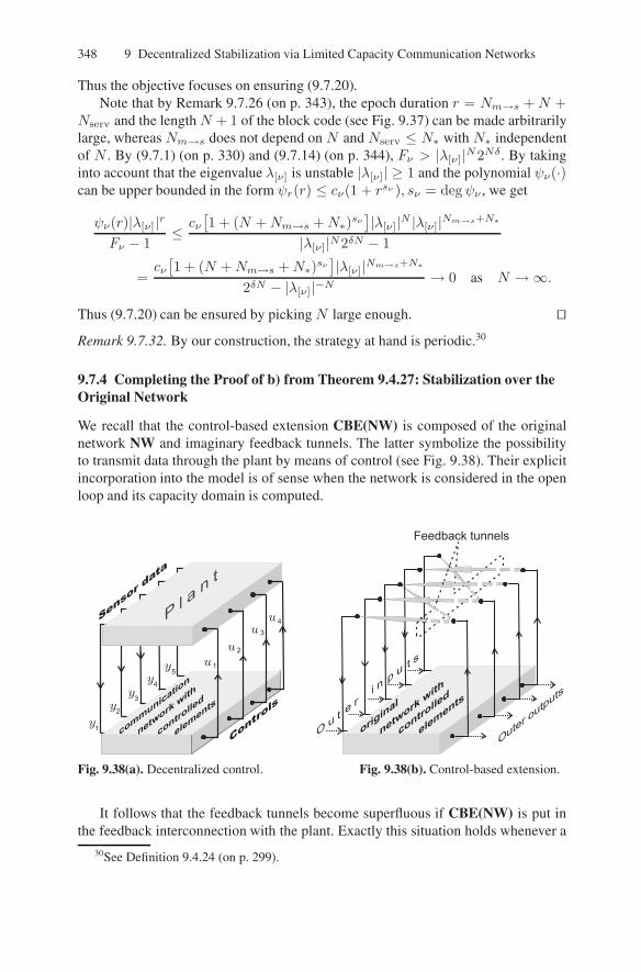
348 9 Decentralized Stabilization via Limited Capacity Communication Networks
Thus the objective focuses on ensuring (9.7.20).Note that by Remark 9.7.26 (on p. 343), the epoch duration r = Nm→s +N +
Nserv and the length N + 1 of the block code (see Fig. 9.37) can be made arbitrarilylarge, whereas Nm→s does not depend on N and Nserv ≤ N∗ with N∗ independentof N . By (9.7.1) (on p. 330) and (9.7.14) (on p. 344), Fν > |λ[ν]|N2Nδ. By takinginto account that the eigenvalue λ[ν] is unstable |λ[ν]| ≥ 1 and the polynomial ψν(·)can be upper bounded in the form ψr(r) ≤ cν(1 + rsν ), sν = degψν , we get
ψν(r)|λ[ν]|rFν − 1
≤ cν[1 + (N +Nm→s +N∗)sν
]|λ[ν]|N |λ[ν]|Nm→s+N∗
|λ[ν]|N2δN − 1
=cν[1 + (N +Nm→s +N∗)sν
]|λ[ν]|Nm→s+N∗
2δN − |λ[ν]|−N→ 0 as N →∞.
Thus (9.7.20) can be ensured by picking N large enough. ⊓⊔Remark 9.7.32. By our construction, the strategy at hand is periodic.30
9.7.4 Completing the Proof of b) from Theorem 9.4.27: Stabilization over theOriginal Network
We recall that the control-based extension CBE(NW) is composed of the originalnetwork NW and imaginary feedback tunnels. The latter symbolize the possibilityto transmit data through the plant by means of control (see Fig. 9.38). Their explicitincorporation into the model is of sense when the network is considered in the openloop and its capacity domain is computed.
Fig. 9.38(a). Decentralized control. Fig. 9.38(b). Control-based extension.
It follows that the feedback tunnels become superfluous if CBE(NW) is put inthe feedback interconnection with the plant. Exactly this situation holds whenever a
30See Definition 9.4.24 (on p. 299).

9.7 Proof of the Sufficiency Part of Theorem 9.4.27 349
stabilizing control strategy for CBE(NW) is considered. Then all data streams thatare interpreted as going through the imaginary feedback tunnels and so virtual can bearranged as real data transmissions by control actions upon the plant (see Fig. 9.39).The corresponding arrangements are proposed in this subsection and result in a sta-bilizing control strategy for the original network NW.
Fig. 9.39(a). Control over CBE(NW). Fig. 9.39(b). Embedding the feedback tun-nels back into the plant.
In this subsection, the stabilizing control strategy for CBE(NW) proposed in theprevious one is said to be initial. When doing the above arrangements, the idealobjective might be to convert this strategy into a control strategy for the originalnetwork NW without any alteration in network outputs (controls) and inputs (ob-servations). Unfortunately, this is impossible since the very idea of communicationby means of control dictates to alter the controls by adding “information carrier”addends:
ui(t) := ubi (t) + ucom
i (t), (9.7.21)
where ubi (t) are initially generated controls organized into control programs Ui(θ).
This also alters the sensor signals.To state the realistic objective, we recall that for the initial control strategy,
• The sensor data are collected during n time steps before the start t = θr of anyepoch θ ≥ 1 and utilized at t = θr by the sensor nodes to compute the prognosisof the observed unstable modes xjα[(θ + 1)r];

350 9 Decentralized Stabilization via Limited Capacity Communication Networks
• The actuator nodes generate control programs
Ui(θ) = colubi [θr], u
bi [θr + 1], . . . , ub
i [(θ + 1)r − 1]
(9.7.22)
for the entire epoch at its beginning θr.
There is no other interaction between the network CBE(NW) and plant.The objective that will be pursued is to alter the control strategy so that
S] The sensor nodes1. Still compute the prognosis xjα[(θ + 1)r] at t = θr;2. Get access to the data initially received over the imaginary feedback tunnels
in another and realistic way; to serve this access, the processing algorithmsat these nodes can be supplemented by additional operations;
3. Process the above data, estimates xjα[(θ + 1)r], and data received via theoriginal network NW just like for the initial strategy;
I] The interior part of the network processes data just like the initial strategy;A] The actuator nodes
1. Process the received data just like for the initial strategy in order to generatethe control programs Ui(θ) at the start of any epoch;
2. Do not send signals into imaginary feedback tunnels but instead, use thesesignals to generate the “communication” addends ucom
i (t) to the controlsfrom A.1];
3. Generate these addends in such a way thata) Their influence on the plant is annihilated at the end of the current epoch:
the controlsucomi [θr], . . ., ucom
i [(θ+1)r−1] drive the unperturbed (ξ(·) ≡0) plant from 0 at t = θr to 0 at t = (θ + 1)r provided that all actuatorsexcept for the ith one are inactive;
b) They are bounded ‖ucomi (t)‖ ≤ cu by a constant cu independent of t, i;
c) The overall controls given by (9.7.21) are zero n time steps before thestart of any epoch.
Remark 9.7.33. Note that S.1] is possible whenever S.2], A.3.a], and A.3.c] hold.
Indeed, A.3.c) implies Assumption 9.7.12 (on p. 337). At the same time, S.2] meansthat at t = θr +Nm→s +N + d (see Fig. 9.37), the sensors still have access to thedata that make them aware about the required controls from A.1]. Due to A.3.a], theireffect on the plant during the entire epoch is identical to that of the overall controls(9.7.21). Thus the latter effect is computable by the sensor nodes, as is required byAssumption 9.7.13 (on p. 338). Hence the remark follows from Proposition 9.7.14(on p. 338).
Lemma 9.7.34. Any control strategy with the features S], I], A] regularly stabilizes31
the plant via the original network NW.
31See Definition 9.4.2 on p. 293.

9.7 Proof of the Sufficiency Part of Theorem 9.4.27 351
Proof. By S], I], and A], this strategy generates just the same control programs Ui(θ)as the initial strategy. At the same time, the “communication addends” from (9.7.21)dot not influence the states x(θr) due to A.3.a]. Since the initial strategy is regularlystabilizing, it follows that the states x(θr) and control programs Ui(θ) are boundedover θ ≥ 0. Thanks to A.3.b], this conclusion is extended on the overall controlsui(t) given by (9.7.21) and t = 0, 1, . . .. Then the standard argument (see, e.g.,(7.8.20) on p. 244) shows that the states x(t) are bounded over t ≥ 0, which com-pletes the proof. ⊓⊔
Converting the initial control strategy into one with the features S], I], and A]comes to arrangements for S.2] and A.2]. To this end, we recall that for the initialstrategy, transmissions over the feedback tunnels were used to communicate (seeFig. 9.40)
1. Side data from the master sensor nodes to their slaves;2. Quantized state prognosis from the sensor nodes to actuator nodes by means of
the basic networked block code BC hosted by CBE(NW);3. Data oi→α driving control generation from the actuators to sensors.
Fig. 9.40. Where the feedback tunnels are used.
Formally, these data are represented by, respectively,
1. A map associating every master sensor with the side data dispatched from thisnode and represented by a binary word of length 2;
2. A map associating every pair sensor-(observed unstable mode xα) with a quan-tized data from the set [1 : Fα];
3. A map associating every pair (actuator i)-(affected unstable mode xα) with areal-valued signal oi→α.
In each case, these data are generated before the transmission is commenced andbelong to a priori known finite sets. (In case 3, this holds since the signals oi→α aregenerated as outputs of the deterministic block code BC driven by the data from 2.)
Since the network CBE(NW) is deterministic, its operation during any of theabove transmissions is uniquely determined by the transmitted data. It follows thatat any time t the message emitted into any feedback tunnel belongs to an a priori

352 9 Decentralized Stabilization via Limited Capacity Communication Networks
known finite set Ri,j(t). Here the pair (i, j) enumerates the tunnel and belongs tothe set (9.4.6) (on p. 294). The corresponding tunnel transmits messages from theactuator node i to the sensor node j with the delay di→j given by (9.4.7) (on p. 294).
Thus the required arrangements focus on making the sensor j aware about thechoice from a known finite set Ri,j(t) that was made by the ith actuator di→j timesteps before. This should be accomplished via generating a proper control ucom
i .A method to achieve this goal was proposed in Subsect. 7.8.1 (starting on p. 233)
for the case of one sensor and actuator. Generalization on the case of several sensorsand actuators is straightforward; the required details are offered further (see p. 353).
According to this method, the initial control strategy hosted by CBE(NW) isconverted into a control strategy hosted by the original NW as follows:
C1) The transmissions over the imaginary feedback tunnels are replaced by• Generating controls at the actuator nodes in the form (9.7.21), where the
first addend on the right is the corresponding entry of the control programfrom A.1], and the second addend is taken from a finite control alphabet andencodes the message initially transmitted over the feedback tunnel;
• Decoding these messages at the sensor nodes on the basis of the prior ob-servations and previously decoded messages.
C2) After the transmissions of all these messages are completed at time tθ = θr +Nm→s +N + d (see Fig. 9.40), the influence of the generated communicationcontrols
U comi = col (ucom
i [θr], . . . , ucomi [tθ − 1])
on the plant is compensated by producing the “remainder” ucomi (t)
∣∣(θ+1)r−1
t=tθso
that A.3.a) be satisfied.
Explanation 9.7.35. The latter is possible due to (9.7.13) (on p. 343). Moreover likein ds.3) on p. 240, the “remainder” can be produced as a function of U com
i so thatucomi [tθ + n] = 0, . . . , ucom
i [(θ + 1)r − 1] = 0.
Remark 9.7.36. Thanks to (9.7.13), the last property implies that the overall controls,i.e., the right-hand sides of (9.7.21), are zero n time steps before the start of anyepoch, which ensures A.3.c) and so by Remark 9.7.33 (on p. 350), S.1].
Remark 9.7.37. The “remainder” from Explanation 9.7.35 assumes finitely manyvalues since it is a function of the element U com
i taken from a finite set. This en-sures A.3.b].
Observation 9.7.38. For the strategy obtained via the above conversion, the claimsS], I], and A] are true. So this strategy regularly stabilizes the plant via the originalnetwork by Lemma 9.7.34.
Observation 9.7.39. By our construction, this strategy is r-periodic.32
Remark 9.7.40. These two observations complete the proof of the a) ⇒ b) part ofTheorem 9.4.27 (on p. 300), provided that C1) is ensured.
We close the section with specifying the technical details related to C.1).32See Definition 9.4.24 (on p. 299).

9.7 Proof of the Sufficiency Part of Theorem 9.4.27 353
Feedback Information Transmission by Means of Control in the Case ofMultiple Sensors and Actuators
Now we deal with not necessarily the above control strategy but any strategy thatsatisfies the following requirements:
R.1) The controls are generated in the form (9.7.21);R.2) At time t = θr, every sensor node j can compute the control programs (9.7.22)
for all actuators i : (i, j) ∈ CVP that affect the observations of this sensor;33
R.3) The claim A.3.c) on p. 350 holds.
The following technical fact [8] is immediate from A.3.c] and (9.4.3) (on p. 292).
Remark 9.7.41. At time θr, θ ≥ 1, any sensor node j can compute the state x(θr)modulo the unobservable subspace L−oj with an accuracyD−oj that depends only onA,Cj and the bounds from (9.4.3).
The following lemma extends Lemma 7.8.4 (on p. 234) on the case of multi-ple sensors and actuators and displays the key fact that enables one to establish therequired feedback communication by means of control.
Lemma 9.7.42. Suppose that R.1)–R.3) hold and a natural numberNi,j is assignedto any feedback tunnel (i.e., any (i, j) ∈ CVP, where CVP is given by (9.4.6) onp. 294). Then for any given sensor j, the related feedback tunnels can be equippedwith finite control alphabets of the respective sizes Ni,j
Ui,j =ui,j(1), . . . , ui,j(Ni,j)
⊂ R
dim(ui) (9.7.23)
so that the following property holds.
• Whenever at a time t = θr + τ ≤ (θ + 1)r − n, θ ≥ 1 the sensor node j isaware of the controls ui(θr), . . . , ui(t − di→j − 1) for all actuators i : (i, j) ∈CVP affecting the observations of this sensor, this node is able to determinethe second addend ucom
i (t − di→j) in (9.7.21) for all concerned i provided thatucomi (t− di→j) ∈ Ui,j ∀i : (i, j) ∈ CVP.
It follows that the sensor is able to determine the serial number s of the correspondingelement ui,j(s) = ucom
i (t−di→j) of the alphabet (9.7.23). Thus the ith actuator cancommunicate any message s ∈ [1 : Ni,j ] to the jth sensor with delay di→j .
Explanation 9.7.43. It is tacitly assumed that the communication controls are chosenfrom Ui,j at not only time t − di,j but also at all previous times to ensure priorcommunications. Then the knowledge of ui(θr), . . . , ui(t − di,j − 1) results fromR.1) and R.2), along with previous decoding.
Proof of Lemma 9.7.42. By Remark 9.7.41, the jth sensor is able to compute anestimate xj(θr) of x(θr) such that
33See Remark 9.7.23 (on p. 343).

354 9 Decentralized Stabilization via Limited Capacity Communication Networks
‖CjAs[xj(θr) − x(θr)]‖ ≤ D−j := ‖Cj‖(‖A‖+ 1)rD−oj (9.7.24)
whenever s ∈ [0 : r]. Now we observe that owing to (9.4.1) and (9.4.2) (on p. 291),
yj(t) = CjAτx(θr)+
τ−1∑
s=0
CjAτ−1−s
[l∑
i=1
Biui(θr + s) + ξ(θr + s)
]+Cjχj(t)
(9.4.6), (9.4.7)====== CjA
τx(θr) +∑
i:(i,j)∈CVP
τ−di→j∑
s=0
CjAτ−1−sBiui(θr + s)
+
τ−1∑
s=0
CjAτ−1−sξ(θr + s) + Cjχj(t)
(9.7.21)===
CjAτ xj(θr) +
∑
i:(i,j)∈CVP
τ−1−di→j∑
s=0
CjAτ−1−sBiui(θr + s)
+∑
i:(i,j)∈CVP
CjAdi→j−1Biu
bi (t− di→j)
+
∑
i:(i,j)∈CVP
CjAdi→j−1Biu
comi (t− di→j)
+
CjA
τ [x(θr) − xj(θr)] +
τ−1∑
s=0
CjAτ−1−sξ(θr + s) + Cjχj(t)
.
Here the discrepancyHj between yj(t) and the first expression in the curly bracketsis computable at the jth sensor node at time t. The norm of the third one is strictlybounded by a constant D[0]
∗ that does not depend on t, θ, j due to (9.4.3) (on p. 292)and (9.7.24). Hence
∥∥∥∥∥∥Hj −
∑
i:(i,j)∈CVP
CjAdi→j−1Biu
comi (t− di→j)
∥∥∥∥∥∥< D
[0]∗ . (9.7.25)
Note that here CjAdi→j−1Bi 6= 0 due to (9.4.7) (on p. 294).Now we put the set i : (i, j) ∈ CVP in order
i1, . . . , ipj
and pick the alpha-
bets (9.7.23) successively for i = i1, . . . , ipj . For i = i1, a finite alphabet (9.7.23)(where i := i1) is chosen so that the points
CjAdi1→j−1Bi1ui1,j(1), . . . , CjA
di1→j−1Bi1ui1,j(Ni1,j)
are 2D[0]∗ -separated.34 Then the control ucom
i1 (t − di1→j) from this alphabet can beuniquely determined from the knowledge of a vector Hj,1 such that
∥∥∥Hj,1 − CjAdi1→j−1Bi1ucomi1 (t− di1→j)
∥∥∥ < D[0]∗ .
34See Definition 7.6.17 (on p. 217).

9.7 Proof of the Sufficiency Part of Theorem 9.4.27 355
After the first alphabet is chosen, (9.7.25) implies
∥∥∥∥∥∥Hj −
∑
i=i2,...,ipj
CjAdi→j−1Biu
comi (t− di→j)
∥∥∥∥∥∥< D
[1]∗
:= D[0]∗ + max
s=1,...,Ni1,j
‖CjAdi1→j−1Bi1ui1,j(s)‖. (9.7.26)
For i = i2, the alphabet (9.7.23) is chosen so that the points
CjAdi2→j−1Bi2ui2,j(1), . . . , CjA
di2→j−1Bi2ui2,j(Ni2,j)
are 2D[1]∗ -separated. Then the control ucom
i2 (t − di2→j) from this alphabet can beuniquely determined from the knowledge of a vector Hj,2 such that
∥∥∥Hj,2 − CjAdi2→j−1Bi2ucomi2 (t− di2→j)
∥∥∥ < D[1]∗ .
Note that (9.7.26) implies
∥∥∥∥∥∥Hj −
∑
i=i3,...,ipj
CjAdi→j−1Biu
comi (t− di→j)
∥∥∥∥∥∥< D
[2]∗
:= D[1]∗ + max
s=1,...,Ni2,j
‖CjAdi2→j−1Bi2ui2,j(s)‖.
By continuing likewise, we construct a sequence D[0]∗ ≤ D
[1]∗ ≤ . . . ≤ D
[pj−1]∗
and the alphabets (9.7.23) for all i = i1, . . . , ipj such that for any s = 1, . . . , pj ,
i) the control ucomis (t − dis→j) from the alphabet Uis→j can be uniquely deter-
mined from the knowledge of a vector Hj,s such that
∥∥Hj,s − CjAdis→j−1Bisucomis (t− dis→j)
∥∥ < D[s−1]∗ . (9.7.27)
ii) the following inequality holds:∥∥∥∥∥∥Hj −
∑
i=is,...,ipj
CjAdi→j−1Biu
comi (t− di→j)
∥∥∥∥∥∥< D
[s−1]∗ . (9.7.28)
For s := pj , (9.7.28) has the form (9.7.27) withHj,pj := Hj known. So ucomis (t−
dis→j) with s = pj can be determined. Then for s = pj − 1, (9.7.28) takes the form(9.7.27) with known
Hj,pj−1 := Hj − CjAdipj→j
−1Bipj ucomipj (t− dipj→j).
This permits us to determine ucomis (t − dis→j) with s = pj − 1. Then we subtract
from Hj the found addends

356 9 Decentralized Stabilization via Limited Capacity Communication Networks
Hj,pj−2 := Hj −∑
i=ipj−1,ipj
CjAdi→j−1Biu
comi (t− di→j)
and find ucomis (t − dis→j) with s = pj − 2. All required controls can be found by
continuing likewise. ⊓⊔Lemma 9.7.42 shows that the actuators can send as much information as desired
by means of control and with the required delays to any given sensor. The next lemmaextends this conclusion to the case where all sensors should receive data simultane-ously.
Lemma 9.7.44. Suppose that R1)–R3) hold and a finite set of messages Mi,j is as-signed to any feedback tunnel, which are enumerated by (i, j) ∈ CVP, where CVPis given by (9.4.6) (on p. 294). Let at any time t ∈ [θr : (θ+1)r−n−d], where θ ≥ 1and d := max(i,j)∈CVP di→j , every actuator i picks messages µi→j(t) ∈ Mi,j toall concerned sensors j, i.e., such that (i, j) ∈ CVP.35
Then each actuator i can be equipped with a rule converting the set of relatedmessages
µi→j(t)j:(i,j)∈CVP
7→ ucomi (t) (9.7.29)
into the second addend from (9.7.21) (on p. 349) so that at any time t ∈ [θr :(θ + 1)r − n] every sensor j can recognize all required messages
µi→j(t− di→j
), i : (i, j) ∈ CVP, t− di→j ≥ θr (9.7.30)
from the knowledge available to this sensor. The conversion rules and the algorithmsof recognition can be chosen independent of θ and t.
Remark 9.7.45. Since the required transmissions from C1) (on p. 352) concern mes-sages taken from a priori-known finite sets according to the discussion precedingC1), Lemma 9.7.44 justifies the possibility of C1) and completes the proof of the a)⇒ b) part of Theorem 9.4.27 (on p. 300) by Remark 9.7.40.
Proof of Lemma 9.7.44. Let every actuator i first convert the set of all dispatchedmessages from (9.7.29) into a compound message µi(t), so that any original messageµi→j(t) from the set and its indices i, j are uniquely reconstructable from µi(t). Thiscompound message will be delivered to every concerned sensor j, where the properpart will be extracted. The message µi(t) can be taken from a specific finite set Mi.
The remainder of the proof involves merely adjusting the arguments from theproof of Lemma 9.7.42 to the current context. In so doing, we pick the control alpha-bets (9.7.23) in a special way. We first observe that due to (9.4.7) (on p. 294),
CjAdi→j−1Bi 6= 0⇔ Li,j := kerCjA
di→j−1Bi 6= Rdim(ui), ∀(i, j) ∈ CVP.
Hence the Lebesgue measure of the linear subspace Li,j is zero; and so is that of theunion
⋃j:(i,j)∈CVP Li,j . Thus for any i, a control ui ∈ Rdim(ui) exists such that
35It is assumed that every message µi→j(t) should be delivered to sensor j with the delaydi→j given by (9.4.7) (on p. 294). We set µi→j(t) := ⊛ for t ∈
`
(θ+1)r−n−d : (θ+1)r´
.

9.7 Proof of the Sufficiency Part of Theorem 9.4.27 357
CjAdi→j−1Biu
i 6= 0, ∀j : (i, j) ∈ CVP. (9.7.31)
To any actuator i = 1, . . . , l, we assign a finite control alphabet Ui =uiµµ∈Mi
whose elements are in a one-to-one correspondence with the messages from Mi andhave the following form:
uiµ = aiµui, where aiµ ∈ R. (9.7.32)
As in the proof of Lemma 9.7.42, these alphabets will be chosen successively fori = 1, . . . , l. For i = 1, the numbers a1
µ, µ ∈M1 are chosen so that the set
CjA
d1→j−1B1u1µ
µ∈M1
is 2D[0]∗ -separated for any sensor j such that (1, j) ∈ CVP. HereD[0]
∗ is the constantfrom (9.7.25). This is possible thanks to (9.7.31) and (9.7.32). The numbers a2
µ, µ ∈M2 are chosen so that the set
CjA
d2→j−1B2u2µ
µ∈M2
is 2D[1]∗ -separated for any sensor j : (2, j) ∈ CVP. Here D[1]
∗ is defined as in(9.7.26) with iν := ν:
D[1]∗ := D
[0]∗ + max
j=1,...,kmaxµ∈M1
∥∥CjAd1→j−1B1u1µ
∥∥ .
Here and throughout, we assume that di→j := 1 if (i, j) 6∈ CVP and note that
CjAdi→j−1Bi = 0, ∀ (i, j) 6∈ CVP (9.7.33)
due to (9.4.6) (on p. 294). The numbers a3µ, µ ∈M3 are chosen so that the set
CjA
d3→j−1B3u3µ
µ∈M3
is 2D[2]∗ -separated for any sensor j : (3, j) ∈ CVP, where
D[2]∗ := D
[1]∗ + max
j=1,...,kmaxµ∈M2
∥∥CjAd2→j−1B2u2µ
∥∥ .
By continuing likewise, we construct a sequence D[0]∗ ≤ · · · ≤ D
[l−1]∗ , control
alphabets Ui =uiµµ∈Mi
for all actuators i, and ensure that the following claimshold:
i) For any actuator i = 1, . . . , l, any control ui ∈ Ui can be uniquely recognizedby any sensor j : (i, j) ∈ CVP from the knowledge of a vector Hi,j such that
∥∥Hi,j − CjAdi→j−1Biui∥∥ < D
[i−1]∗ ;

358 9 Decentralized Stabilization via Limited Capacity Communication Networks
ii) The numbersD[i]∗ are related by the recursion
D[i]∗ := D
[i−1]∗ + max
j=1,...,kmaxµ∈Mi
∥∥CjAdi→j−1Biuiµ
∥∥ . (9.7.34)
Finally, we introduce the following conversion rule of the form (9.7.29)µi→j(t)
j:(i,j)∈CVP
7→ µi(t) 7→ ucomi (t) := uiµi(t)
(t) ∈ Ui. (9.7.35)
To complete the proof, we show that for any t ∈ [θr : (θ + 1)r − n], anysensor can recognize all required messages (9.7.30) and the controls ui(t − di→j)with (i, j) ∈ CVP from the knowledge available to this sensor. The proof will be byinduction on t = θr, θr + 1, . . ..
For t = θr, the claim is evident: Since n ≥ di→j ≥ 1 by (9.4.7) (on p. 294),no message from (9.7.30) should be recognized and ui(t − di→j) = 0 by R3) (onp. 353). Let the claim be true for all times t′ ≥ θr not exceeding t − 1, wheret ∈ (θr : (θ + 1)r − n]. By retracing the arguments underlying (9.7.25) with regardto (9.7.33), we see that
∥∥∥∥∥Hj −l∑
i=1
CjAdi→j−1Biu
comi (t− di→j)
∥∥∥∥∥ < D[0]∗ ,
where Hj is a vector computable from the knowledge available to sensor j. Then(9.7.34) and (9.7.35) imply that
∥∥Hi,j − CjAdi→j−1Biucomi (t− di→j)
∥∥ < D[i−1]∗ ,
whereHi,j := Hj −
∑
i′>i
CjAdi′→j−1Bi′u
comi′ (t− di′→j).
By putting i := l here with regard to (9.7.33) and i), we see that sensor j can recog-nizeCjAdl→jBlu
coml (t−dl→j) and if (l, j) ∈ CVP, the control ucom
l (t−dl→j). Af-ter this, the sensor acquires the knowledge ofHl−1,j . Then by considering i := l−1likewise, we see that sensor j can compute CjAd(l−1)→jBl−1u
coml−1 (t − d(l−1)→j)
and if (l− 1, j) ∈ CVP, the control ucoml−1 (t− d(l−1)→j). The proof is completed by
continuing likewise. ⊓⊔
9.8 Proofs of the Lemmas from Subsect. 9.5.2 and Remark 9.4.28
9.8.1 Proof of Lemma 9.5.6 on p. 303
(i) is immediate from Definition 9.5.5 (on p. 303).(ii) Let BC denote the corresponding networked block code, and N and rcode =
rT T∈T stand for its length and rate ensemble, respectively. We recall that BCis an admissible data processing strategy A ∈ A considered on the time interval
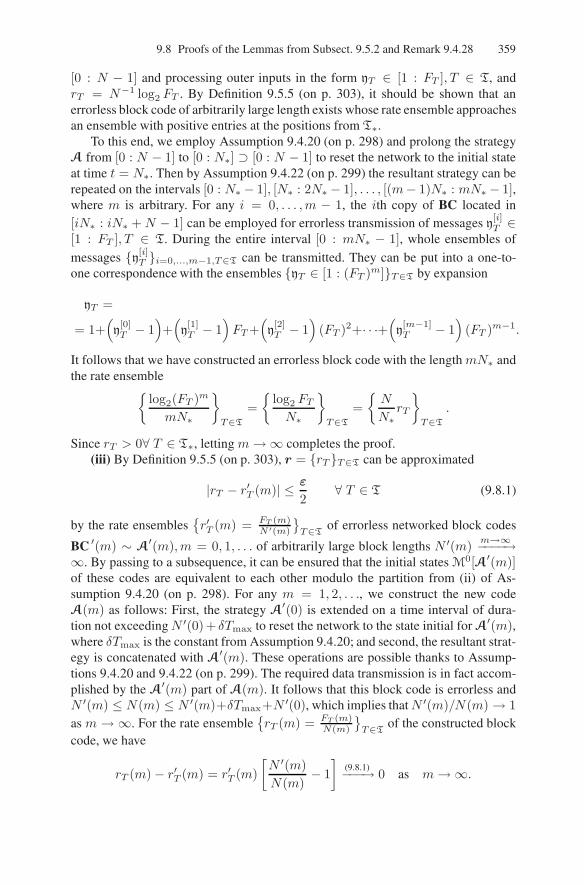
9.8 Proofs of the Lemmas from Subsect. 9.5.2 and Remark 9.4.28 359
[0 : N − 1] and processing outer inputs in the form yT ∈ [1 : FT ], T ∈ T, andrT = N−1 log2 FT . By Definition 9.5.5 (on p. 303), it should be shown that anerrorless block code of arbitrarily large length exists whose rate ensemble approachesan ensemble with positive entries at the positions from T∗.
To this end, we employ Assumption 9.4.20 (on p. 298) and prolong the strategyA from [0 : N − 1] to [0 : N∗] ⊃ [0 : N − 1] to reset the network to the initial stateat time t = N∗. Then by Assumption 9.4.22 (on p. 299) the resultant strategy can berepeated on the intervals [0 : N∗ − 1], [N∗ : 2N∗ − 1], . . . , [(m− 1)N∗ : mN∗ − 1],where m is arbitrary. For any i = 0, . . . ,m − 1, the ith copy of BC located in[iN∗ : iN∗ +N − 1] can be employed for errorless transmission of messages y
[i]T ∈
[1 : FT ], T ∈ T. During the entire interval [0 : mN∗ − 1], whole ensembles of
messages y[i]T i=0,...,m−1,T∈T can be transmitted. They can be put into a one-to-
one correspondence with the ensembles yT ∈ [1 : (FT )m]T∈T by expansion
yT =
= 1+(y[0]T − 1
)+(y[1]T − 1
)FT+
(y[2]T − 1
)(FT )2+· · ·+
(y[m−1]T − 1
)(FT )m−1.
It follows that we have constructed an errorless block code with the lengthmN∗ andthe rate ensemble
log2(FT )m
mN∗
T∈T
=
log2 FTN∗
T∈T
=
N
N∗rT
T∈T
.
Since rT > 0∀ T ∈ T∗, letting m→∞ completes the proof.(iii) By Definition 9.5.5 (on p. 303), r = rT T∈T can be approximated
|rT − r′T (m)| ≤ ε
2∀ T ∈ T (9.8.1)
by the rate ensemblesr′T (m) = FT (m)
N ′(m)
T∈T
of errorless networked block codes
BC ′(m) ∼ A′(m),m = 0, 1, . . . of arbitrarily large block lengths N ′(m)
m→∞−−−−→∞. By passing to a subsequence, it can be ensured that the initial states M0[A′(m)]of these codes are equivalent to each other modulo the partition from (ii) of As-sumption 9.4.20 (on p. 298). For any m = 1, 2, . . ., we construct the new codeA(m) as follows: First, the strategy A
′(0) is extended on a time interval of dura-tion not exceedingN ′(0)+ δTmax to reset the network to the state initial for A
′(m),where δTmax is the constant from Assumption 9.4.20; and second, the resultant strat-egy is concatenated with A
′(m). These operations are possible thanks to Assump-tions 9.4.20 and 9.4.22 (on p. 299). The required data transmission is in fact accom-plished by the A
′(m) part of A(m). It follows that this block code is errorless andN ′(m) ≤ N(m) ≤ N ′(m)+δTmax+N ′(0), which implies thatN ′(m)/N(m)→ 1
as m → ∞. For the rate ensemblerT (m) = FT (m)
N(m)
T∈T
of the constructed blockcode, we have
rT (m)− r′T (m) = r′T (m)
[N ′(m)
N(m)− 1
](9.8.1)−−−→ 0 as m→∞.

360 9 Decentralized Stabilization via Limited Capacity Communication Networks
Since the block codes ∼ A(m) have a common initial state by construction, theproof is completed by invoking (9.8.1). ⊓⊔
9.8.2 Proof of Lemma 9.5.8 on p. 304
The second inclusion from (9.5.22) (on p. 305) is evident. To prove the first one, wepick an element rα from the set on the left. By (9.5.22), an ensemble
r = rα,i(α,i)∈Tmw ∈ CD[PREFmw ⊞ CBE(NW)Tmw
]
exists such that rα =∑i∈Imw→α
rα,i ∀α. Let 0 < δ < min(α,i):rα,i 6=0 rα,i and N =1, 2, . . . be given. By Definition 9.5.5 (on p. 303), there exists an errorless networkedblock code BC hosted by and serving the above network and transmission scheme,respectively, with block length N ≥ N whose rate ensemble (9.5.19) (on p. 303)approaches r with accuracy δ.
Now we construct a block code BCnew serving PREFmw⊞CBE(NW)⊞SUFFqmw
and transmitting constant messages µα ∈ [1 : Fα] from the source to the output node∼ xα for all α. Here Fα :=
∏i∈Imw→α
Fα,i. Specifically when receiving the messageµα from the source ∼ xα, any sensor node j ∈ Jmw←α expands it in the form
µα = µα,i1α + Fα,i1α(µα,i2α − 1) + Fα,i1αFα,i2α(µα,i3α − 1) + · · ·· · ·+ Fα,i1α · · ·Fα,ipα−1
α(µα,ipα
α− 1), µα,iσα ∈ [1 : Fα,iσα ] (9.8.2)
and interprets µα,iσ as the individual message from the source ∼ xα to the outputnode i = iσ, thus creating the situation where BC can operate. Here i1α, . . . , ipα
α is an enumeration of Imw→α. The signals µα,i are processed by the rules of BC. Soevery signal µα,i is correctly decoded at time N − 1 at the actuator node i. Intothe additive channel from SUFFq
mw going to the output node ∼ xα, the actuatornode emits the corresponding addend from (9.8.2). The addition is performed by thechannel. So the correct message arrives at the output node ∼ xα, and an errorlessBCnew is constructed. The entries of its rate vector (9.4.13) (on p. 298)
log2 FαN
=∑
i∈Imw→α
log2 Fα,iN
approach those rα =∑i∈Imw→α
rα,i of rα with accuracy≤ δ|Imw→α|, where δ > 0 isarbitrary. The proof is completed by invoking Definition 9.4.17 (on p. 298). ⊓⊔
9.8.3 Proof of Lemma 9.5.10 on p. 306
(i) Let r = rαn+
α=1 belong to the set in the left-hand side of (9.5.25), and δ >0, N = 1, 2, . . . be given. By Definition 9.4.17 (on p. 298), an errorless BC hostedby PREFmw ⊞ CBE(NW) ⊞ SUFF+
mw with block length N ≥ N exists whose ratevector (9.4.13) (on p. 298) approaches r with accuracy δ.

9.8 Proofs of the Lemmas from Subsect. 9.5.2 and Remark 9.4.28 361
We are going to transform it into a code BCnew serving PREFmw ⊞CBE(NW)⊞SUFF
+
mw. To this end, we introduce an enumeration Gν = i1ν, . . . , ipνν for any ν.
For BCnew, the νth source produces a constant message µν ∈ [1 : F ν ], whereF ν :=
∏α∈Gν
Fα and Fα is the size of the alphabet of the source ∼ xα. On gettingaccess to this message, each sensor node j ∈ Jmw←α (with α ∈ Gν) expands it in theform (9.8.2) (where α := ν and Fν,i := Fi). The quantities µν,iφν are interpreted
as messages from the node α = iφν , φ = 1, . . . , pν of BC. These messages are thenprocessed by the rules of the original BC. So at t = N − 1, the message µν,α iscorrectly decoded by the output node∼ xα. This node collects information from theactuator nodes i ∈ Imw
→α, which are common for all modes α ∈ Gν within a givengroup. Since the channels from SUFF+
mw have the maximal possible cardinalities,all data from the above actuator nodes can be removed to the single representativeof the group of output nodes ∼ xα, α ∈ Gν retained in SUFF
+
mw as compared withSUFF+
mw. It follows that all messages µν,α with α ∈ Gν can be correctly decoded atthis node. The original message µν is restored by (9.8.2). Thus an errorless BC
new
is constructed.The entries of its rate vector (9.4.13) (on p. 298)
log2 F νN
=∑
α∈Gν
log2 FαN
approach those of the vector∑
α∈Gνrαsν=1
with accuracy ≤ δmaxν |Gν |. Let-ting δ → 0 shows that the domain in the left-hand side of (9.5.25) (on p. 306) is asubset of that in the right-hand side by Definition 9.4.17 (on p. 298).
Conversely, let r = rαn+
α=1 belong to the set in the right-hand side of (9.5.25)(on p. 306), and let 0 < δ < minα:rα>0 rα, N = 1, 2, . . . be given. By Def-inition 9.4.17 (on p. 298), an errorless block code BC hosted by PREFmw ⊞
CBE(NW)⊞SUFF+
mw
log2 Fν
N
sν=1
approaches the vector∑
α∈Gνrα
sν=1
with accuracy δ. We are going to transform
it into a code BCnew hosted by PREFmw ⊞ CBE(NW) ⊞ SUFF+mw.
Let the source∼ α of PREFmw produce constant messages µα ∈ [1 : Fα], whereFα := max
⌊2(rα−δ)N⌋; 1
. Any sensor node j ∈ Jmw
←α, α ∈ Gν has access to allmessages µα′ coming from the same group of input nodes α′ ∈ Gν . So all thesesensor nodes may convert these messages into the common natural µν by (9.8.2)(modified just as in the first part of the proof). Then µν is interpreted as a commonmessage broadcasted from the source ∼ ν, as is required by PREFmw. Moreover,this message is a legal input for BC since
µν ≤∏
α∈Gν
Fα ≤∏
α∈Gν
⌊2(rα−δ)N
⌋≤⌊2N(
Pα∈Gν
rα−δ|Gν |)⌋≤ F ν .
The messages µν are then processed by the rules of BC and thus are correctly de-coded at the output node∼ ν from the data received over the corresponding channel
with block lengthN≥ N exists whose rate vector

362 9 Decentralized Stabilization via Limited Capacity Communication Networks
of SUFF+
mw. The clones of this channel are all channels from SUFF+mw arriving at the
nodes∼ xα, α ∈ Gν . So at any of the latter nodes, µν can also be correctly decodedand thus µα can be correctly restored via the expansion (9.8.2). Thus an errorlessBCnew is constructed.
For the entries of its rate vector (9.4.13) (on p. 298), we have
log2 FαN
= max
log2⌊2(rα−δ)N⌋
N; 0
∈[
log2 max2(rα−δ)N − 1; 1
N,max rα − δ; 0
].
Since δ < rα whenever rα > 0, the ends of this interval are close to rα for N ≈ ∞and δ ≈ 0. It follows that the domain in the right-hand side of (9.5.25) is a subset ofthat in the left-hand side by Definition 9.4.17, which completes the proof.
(ii) Modulo apparent technical details, the proof is similar to that of (i). ⊓⊔
9.8.4 Proof of Remark 9.4.28 on p. 300
To prove this remark, we basically repeat the arguments from the proof of the ne-cessity part of Theorem 9.4.27 (on p. 300) given in Sect. 9.6. This proof derived therequired claim d) from stability under zero noises and stable modes. In other words,the stability assumption of c) was utilized only partly. Now we consider a more gen-eral situation where the plant noises may be nonzero within the first m time steps:
ξ(t) ≡ 0 ∀t ≥ m, χj(t) ≡ 0, ξα(t) = 0, x0α = 0 ∀t ≥ 0, α ≤ 0. (9.8.3)
So the sequence of the plant noises is of the form
Ξ = ξ(0), ξ(1), . . . , ξ(m− 1), 0, 0, . . ., ξ(t) ∈Munst(A). (9.8.4)
Retracing Steps 1 and 2 of the Initial Proof
They are retraced with the following modifications.Step 1 (see Subsect. 9.6.2 starting on p. 325).
m.1) Unlike (i) on p. 324, the sources (associated with unstable modes xα) producenot only the matching mode x0
α of the initial state but also the relevant partΞ[ν] := [ξ(t)][ν]t≥0 of the noise sequence (9.8.4). Here ν := ν(α) is theserial number of the group from (9.4.8) (on p. 295) containing xα.
m.2) The rule (9.6.4) (on p. 326) to restore the observation from the data currentlyavailable at the jth sensor node is modified as follows:
yj(t) = Cj
Atx0
j+
∑
i:(i,j)∈CVP
t−di→j∑
θ=0
At−1−θBiui(θ)
+
t−1∑
θ=0
At−1−θξj(θ)
.

9.8 Proofs of the Lemmas from Subsect. 9.5.2 and Remark 9.4.28 363
Explanation 9.8.1. We recall that x0j is the vector of the data received by the jth
sensor node from all initial sources of NW1. This vector has the form (9.4.8) (onp. 295), where all missing data are substituted by zeros and all modes received fromthe sourcers are put in the proper places. The vector ξj(θ) is the similar partial re-construction of the entry ξ(t) from (9.8.4) based on the available source data.
Observation 9.8.2. Since the above formula restores the observations correctly,Lemma 9.6.4 (on p. 326) remains true with (9.8.3) substituted in place of (9.6.1).
Step 2 (see Subsect. 9.6.3 starting on p. 326).
• The operation of the actuator nodes is changed as was discussed in Observa-tion 9.6.9 (on p. 328).
With regard to the necessity to take into account the extra term
t−1∑
θ=0
At−1−θξ(θ)
in (9.6.7), the conclusion of this observation now transforms as follows:Atx0 +
t−1∑
θ=0
At−1−θξ(θ) −∑
i∈Imw→α
xu,i(t)
α
∈ [−D∞, D∞] ∀α, t. (9.8.5)
We recall that D∞ denotes the supremum (9.4.4) (on p. 292).As a result, the following claim is established.
Lemma 9.8.3. Suppose that the network NW 1 := PREFmw ⊞ CBE(NW) is fedby the inputs described in m.1) on p. 362. Then this network can be equipped withan admissible data processing strategy such that the outputs xu,i(t) of the actuatornodes (marked by i) satisfy (9.8.5) whenever (9.8.3) holds and ‖x0‖ ≤ Dx, ‖ξ(t)‖ ≤D, where Dx, D are taken from (9.4.3) (on p. 292).
Errorless Block Code for the Network PREFmw ⊞ CBE(NW) with theCommunication Scheme Tmw
Now we consider the prefix PREFmw and the data communication scheme Tmw in-troduced on p. 307. We recall that the data sources of this prefix are associated withthe subspaces from (9.5.26) (on p. 307) and enumerated by ν = 1, . . . , g. In accor-dance with the scheme Tmw, data should be transmitted from any such source∼Mν
to all actuators i that control the subspace Mν .
Lemma 9.8.4. For any ν, there exists i = iν such that (ν, iν) ∈ Tmw and the capac-ity domain CD[PREFmw ⊞ CBE(NW)Tmw] contains a rate ensemble rT T∈Tmw
with rν,iν > 0∀ ν.

364 9 Decentralized Stabilization via Limited Capacity Communication Networks
Proof. Let ν be chosen. By applying Lemma 7.6.7 (on p. 212) to the plant x[ν](t +1) = A|Mνx[ν](t) + ξ[ν](t), we see that m and two admissible disturbances
Ξs[ν] = ξs[ν](0), ξs[ν](1), . . . , ξs[ν](m− 1), 0, 0, . . ., ‖ξs[ν](θ)‖ ≤ D, s = 1, 2
exist that drive this plant from 0 at t = 0 to the states xs[ν](m) at t = m such that
‖x1[ν](m) − x2
[ν](m)‖ > 2D∞. Since we deal with the norm ‖ · ‖ := ‖ · ‖∞in thischapter, an unstable mode xα exists such that
‖x1α(m)− x2
α(m)‖ > 2D∞, ν(α) = ν. (9.8.6)
Note that Imw→α = Imw→ν(α), where Imw→ν is the set of actuators controlling thesubspace Mν (see p. 307). So thanks to (9.8.5) and (9.8.6), the number s = 1, 2 isrecognizable from the knowledge of
∑
i∈Imw→ν
xu,i(t) (9.8.7)
provided that the block code from Lemma 9.8.3 is fed by x0 := 0 and Ξs[ν] at anyinput node∼ xα such that ν(α) = ν, whereas all other nodes are fed by Ξ[ν(α)] := 0.Then all input nodes from any group in (9.4.8) (on p. 295) are fed by identical data.These nodes are departing points for the cloned channels from PREFmw. So all thesechannels except for one may be discarded, which transforms PREFmw into PREFmw.The source ∼ ν produces s = 0, 1; the conversion s 7→ Ξs[ν] is performed at therelated sensor nodes. All other sources produce the output 1, which is converted intothe zero sequence at any concerned sensor node.
Since s is recognizable from the sum (9.8.7), it can be also recognized from theknowledge of some addend xu,i(t), i = iν ∈ I→ν . By doing so, we obtain a blockcode transmitting without an error one bit from ν to iν , and zero bits from ν′ to i′ forall other pairs (ν′, i′) ∈ Tmw. The network initial state for this code is identical tothat for the strategy from Lemma 9.8.3. By invoking Assumption 9.4.20 (on p. 298),we prolong the block code to reset the network to this initial state. After this the blockcodes related to ν = 1, . . . , g can be concatenated to form a block code transmittingwithout an error one bit from ν to iν for all ν, and zero bits from ν′ to i′ for the otherpairs (ν′, i′) ∈ Tmw. The proof is completed by (ii) of Lemma 9.5.6 (on p. 303). ⊓⊔
Completion of the Proof of Remark 9.4.28 on p. 300
By (ii) of Lemma 9.5.10 (on p. 306) and Lemma 9.8.4, the capacity domainCD[PREFmw ⊞ CBE(NW)Tmw
]contains a rate ensemble rα,i(α,i)∈Tmw such
that rα,iν > 0 for all α ∈ Gν and ν = 1, . . . , g. Here Gν is the νth group of modesfrom (9.4.8) (on p. 295). Then the first inclusion from (9.5.22) (on p. 305) impliesthat CD
[PREFmw ⊞ CBE(NW) ⊞ SUFFq
mw
]contains a rate vector with positive en-
tries, which completes the proof. ⊓⊔

10
H∞ State Estimation via Communication Channels
10.1 Introduction
One approach to the problem of state estimation via limited capacity communicationchannels was proposed in [220] and developed in [45, 100, 132, 133, 184] (see alsoChaps. 2–7 of this book). In this framework, the observation must be coded intoa sequence of finite-valued symbols and transmitted via a digital communicationchannel. With the approach of [45, 100, 133, 184], classic Kalman and H∞ stateestimation theory cannot be applied since the estimator only observes the transmittedsequence of finite-valued symbols. In fact, we need to design a hybrid dynamicalsystem that consists of two subsystems. The first subsystem, which is called coder,receives real-valued measurements and converts them into a finite-valued symbolicsequence that is sent over the limited capacity communication channel. The secondsubsystem (decoder) receives this symbolic sequence and converts it into a real-valued state estimate. In other words, such state estimators with bit-rate constraintsform an important subclass of so-called hybrid dynamic systems. In general, hybridsystems are those that combine continuous and discrete event dynamics and involveboth real and symbolic variables; see, e.g., [104, 174, 177, 185, 211].
Another approach was proposed in [175] where the bandwidth limitation con-straint was modeled in a manner that the state estimator can communicate withonly one of several sensors at any time instant (this approach will be presented inChaps. 14 and 15 of this book). The main disadvantage of both these approaches isthat the state estimation systems proposed in [45, 100, 132–135, 175, 184, 220, 221]are highly nonlinear and contain symbolic variables. In this chapter, we propose anew problem statement. In our new problem statement, the communication chan-nel transmits a continuous time vector signal. The limited capacity of the channelmeans that the dimension of the signal transmitted by the channel is smaller thanthe dimension of the measured output of the system. Our goal is to design a lineartime-invariant coder that transforms the measured output into the signal to be trans-mitted and a linear time-invariant decoder that transforms the transmitted signal intothe state estimate. This approach simplifies the problem and allows for obtainingmore constructive and understandable results. The main advantage is that estimation
A.S. Matveev and A.V. Savkin, Estimation and Control over Communication Networks,
© Birkhäuser Boston, a part of Springer Science + Business Media, LLC 200
365 doi: 10.1007/978-0-8176-4607-3_10,
9

366 10 H∞ State Estimation via Communication Channels
system obtained in this chapter is linear and time-invariant. This allows for applyingconventional linear control theory to the problem of state estimation with bandwidthlimitation constraints. Unlike [45,132,133,220] where the Kalman filtering problemwas considered and [100, 175, 184] where the set-valued approach to state estima-tion was employed, in this chapter we consider the case of H∞ state estimation.The main result of the chapter shows that the linear H∞ control theory when suit-ably modified provides a good framework for the problem of limited communicationstate estimation. This result was originally published in [168].
It should be pointed out that the proposed state estimation method is computa-tionally nonexpansive and easy to implement in real time. The obtained results canbe extended to the case of uncertain linear systems.
The remainder of the chapter is organized as follows. In Sect. 10.2, we introducethe class of systems under consideration. The main results of the chapter and theirproofs are given in Sect. 10.3.
10.2 Problem Statement
We consider the linear system defined on the infinite time interval [0,∞):
x(t) = Ax(t) +Bw(t); x(0) = 0;
z(t) = Kx(t);
y(t) = Cx(t) + v(t), (10.2.1)
where x(t) ∈ Rn is the state; w(t) ∈ Rp and v(t) ∈ Rl are the disturbance in-puts; z(t) ∈ Rq is the estimated output, and y(t) ∈ Rl is the measured output, andA,B,K , and C are given matrices.
The state estimation problem is to find an estimate z of z in some sense usingthe measurement of y. One of the most common frameworks for the state estima-tion problem is based on the H∞ theory. More precisely, the problem of H∞ stateestimation can be stated as follows; e.g., see [14, 66, 130]:
Given a constant γ > 0, find a causal unbiased filter z(t) = F [t, y(·) |t0] if itexists such that
J := sup[w(·),v(·)]∈L2[0,∞)
‖z(·)− z(·)‖22‖w(·)‖22 + ‖v(·)‖22
< γ2. (10.2.2)
Let m < l be given. We will consider the problem of H∞ state estimation via acommunication channel of dimension m.
Suppose estimates of the output z(t) are required at a distant location and areto be transmitted via a limited capacity communication channel such that only mreal numbers may be sent at each time t. We consider a system that consists of thecoder, the transmission channel, and the decoder. Using the measurement y(·) |t0,the coder produces a vector y(t) of dimension m that is transmitted via the channeland then received by the decoder. In its turn, the decoder produces an estimate z(t)
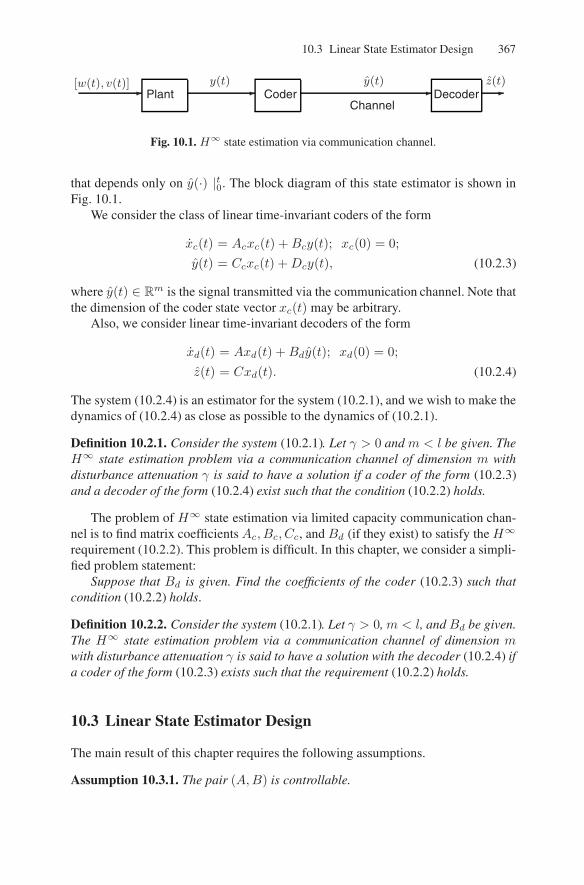
10.3 Linear State Estimator Design 367
-
[w(t), v(t)]Plant -
y(t)Coder -
y(t)
ChannelDecoder -
z(t)
Fig. 10.1. H∞ state estimation via communication channel.
that depends only on y(·) |t0. The block diagram of this state estimator is shown inFig. 10.1.
We consider the class of linear time-invariant coders of the form
xc(t) = Acxc(t) +Bcy(t); xc(0) = 0;
y(t) = Ccxc(t) +Dcy(t), (10.2.3)
where y(t) ∈ Rm is the signal transmitted via the communication channel. Note thatthe dimension of the coder state vector xc(t) may be arbitrary.
Also, we consider linear time-invariant decoders of the form
xd(t) = Axd(t) +Bdy(t); xd(0) = 0;
z(t) = Cxd(t). (10.2.4)
The system (10.2.4) is an estimator for the system (10.2.1), and we wish to make thedynamics of (10.2.4) as close as possible to the dynamics of (10.2.1).
Definition 10.2.1. Consider the system (10.2.1). Let γ > 0 and m < l be given. TheH∞ state estimation problem via a communication channel of dimension m withdisturbance attenuation γ is said to have a solution if a coder of the form (10.2.3)and a decoder of the form (10.2.4) exist such that the condition (10.2.2) holds.
The problem of H∞ state estimation via limited capacity communication chan-nel is to find matrix coefficientsAc, Bc, Cc, and Bd (if they exist) to satisfy the H∞
requirement (10.2.2). This problem is difficult. In this chapter, we consider a simpli-fied problem statement:
Suppose that Bd is given. Find the coefficients of the coder (10.2.3) such thatcondition (10.2.2) holds.
Definition 10.2.2. Consider the system (10.2.1). Let γ > 0,m < l, andBd be given.The H∞ state estimation problem via a communication channel of dimension mwith disturbance attenuation γ is said to have a solution with the decoder (10.2.4) ifa coder of the form (10.2.3) exists such that the requirement (10.2.2) holds.
10.3 Linear State Estimator Design
The main result of this chapter requires the following assumptions.
Assumption 10.3.1. The pair (A,B) is controllable.

368 10 H∞ State Estimation via Communication Channels
Assumption 10.3.2. The pair (A,K) is observable.
Assumption 10.3.3. The pair (A,C) is observable.
Our solution to the above problem involves the following Riccati algebraic equa-tions:
AY + Y A T + Y
[1
γ2K TK − C TC
]Y +BB T = 0, (10.3.5)
A TXǫ +XǫA+Xǫ
[1
ǫBdB
Td −
1
γ2BB T
]Xǫ +K TK = 0. (10.3.6)
Now we are in a position to present the main result of this chapter.
Theorem 10.3.4. Consider the system (10.2.1), suppose that Assumptions 10.3.1–10.3.3 hold, and that the coefficient Bd of the decoder (10.2.4) is given. Let γ > 0be a given constant and m be a given integer. Then, the following statements areequivalent:
(i) The H∞ state estimation problem via a communication channel of dimensionm with disturbance attenuation γ has a solution with the decoder (10.2.4).
(ii) A constant ǫ > 0 exists such that the algebraic Riccati equations (10.3.5) and(10.3.6) have stabilizing solutions Y ≥ 0 and Xǫ ≥ 0 such that ρ(Y Xǫ) < γ2
where ρ(·) denotes the spectral radius of a matrix.
Furthermore, suppose that condition (ii) holds. Then, the coder (10.2.3) with
Ac =
(Ac −BcC−BCc A
); Bc =
(Bc0
); Cc =
(Cc 0
);
Ac = A+BCc − BcC +1
γ2BB TXǫ;
Bc =
[I − 1
γ2Y Xǫ
]−1
Y C T, Cc =1
ǫB TdXǫ (10.3.7)
solves the H∞ state estimation problem via a communication channel of dimensionm with disturbance attenuation γ with the decoder (10.2.4).
Proof of Theorem 10.3.4: Statement (i)⇒ (ii). Assume that condition (i) holds,and consider the decoder (10.2.4). Introduce a new vector variable x := x(t)−xd(t).Then x(t) satisfies the equation
˙x(t) = Ax(t) +By(t) +Bw(t); x(0) = 0. (10.3.8)
Furthermore, introduce
z(t) := Kx(t); y(t) := Cx(t) + v(t). (10.3.9)
Now consider the linear system (10.3.8), (10.3.9) and suppose that y(t) is the controlinput, w(t) and v(t) are the disturbance inputs, y(t) is the measured output, and z(t)is the controlled output. The requirement (10.2.2) can now be rewritten as

10.3 Linear State Estimator Design 369
J := sup[w(·),v(·)]∈L2[0,∞)
‖z(·)‖22‖w(·)‖22 + ‖v(·)‖22
< γ2. (10.3.10)
Now the coder (10.2.3) can be considered as an output feedback controller withinput y(·) and output y(·). Furthermore, this controller solves the output feedbackH∞ control problem (10.3.10). Note that the H∞ control problem (10.3.10) is asingular problem. The approach taken to solve this singular problem is a perturbationapproach such as contained in [81]. As it was shown in [81], since the controller(10.2.3) solves the H∞ control problem (10.3.10), a small ǫ > 0 exists such that thesame controller solves the nonsingularH∞ control problem
J := sup[w(·),v(·)]∈L2[0,∞)
‖z(·)‖22 + ǫ‖y(·)‖22‖w(·)‖22 + ‖v(·)‖22
< γ2. (10.3.11)
Now condition (ii) follows from the standard H∞ control theory; e.g., see [151],p.73. This completes the proof of this part of the theorem.
Statement (ii)⇒ (i). Suppose that condition (ii) holds. Then, it follows from thestandard H∞ control theory (e.g., see [151], pp. 73 and 78) that the linear outputfeedback controller
˙xc(t) = Acxc(t) + Bcy(t); xc(0) = 0;
y(t) = Ccxc(t) (10.3.12)
with the coefficients defined by (10.3.7) solves theH∞ control problem (10.3.11) forthe system (10.3.8), (10.3.9). Since z = z− z, the H∞ requirement (10.2.2) followsfrom (10.2.2). Furthermore, since y(t) = y(t) − Cxd(t) and xd(t) is defined by(10.2.4), (10.3.12) can be rewritten in the form (10.2.3) with the coefficients definedby (10.3.7). This completes the proof of Theorem 10.3.4.

11
Kalman State Estimation and Optimal Control Basedon Asynchronously and Irregularly DelayedMeasurements
11.1 Introduction
In this chapter, we study discrete-time linear partially observed systems with Gaus-sian disturbances. Various sensor signals or even parts of a sensor output are com-municated to the observer or controller over parallel channels with independent de-lays. Messages may arrive out of order; there may be periods when no informationis received. Data transferred via a channel may be corrupted or even lost due to,e.g., noise in the communication medium and protocol malfunctions. The situationis complicated by the fact that many communication channels do not satisfy the timeinvariance condition [208, 232]. The reasons for it vary depending on the type of thechannel. In some cases, this may be due to the relative motion of the transmitter andthe receiver, as well as due to oscillator drifts and phase noise coupled with multipatheffects [208]. For digital networked channels, the origins of the phenomenon may betraced back, in particular, to competition between channels for the network resources.As a result, the prognosis of the future states of the communication medium is often ahard task; and we suppose that the statistics of the transmission delays is not known.At the same time, it is characteristic of many channels that each message transferredis marked with a “time stamp” indicating the moment of the transfer beginning; andwe assume this.
The minimum variance state estimation problem is solved and an analog of theKalman filter is proposed. For a finite horizon linear-quadratic Gaussian (LQG) op-timal control problem, we obtain the solution in the form of the above filter coupledwith the controller optimal in the deterministic linear-quadratic optimization prob-lem. We also derive the solution for the infinite-horizon problem of minimizing theaverage cost per unit time. To this end, we introduce a concept of observability viacommunication channels that may lose data. A number of criteria for such an ob-servability are offered. The main results of this chapter were originally presentedin [105, 106].
When dealing with the state estimation problem, we suppose that the controlstrategy is given. We also assume that there may be a difference between the controlcurrently produced by the controller and that acting upon the plant. This difference
A.S. Matveev and A.V. Savkin, Estimation and Control over Communication Networks,
© Birkhäuser Boston, a part of Springer Science + Business Media, LLC 200
371 doi: 10.1007/978-0-8176-4607-3_11,
9

372 11 Kalman State Estimation and Optimal Control Based on Delayed Measurements
may be caused by a variety of reasons, e.g., the noise, delays, and data dropout in thecontrol loop. At the same time, this chapter addresses the optimal control problems inthe case where the control loop is perfect; i.e., the control generated by the controlleracts upon the plant immediately and with no distortion. Generalizations on the caseof nonperfect control loop will be considered in the next chapter, and in doing so, theresults on the state estimation from this chapter will be employed.
The issue of state estimation and control over communication channels with datadropouts and delays was addressed in, e.g., [13, 72, 92, 93, 97, 98, 131, 146, 163, 186,187, 194–196, 209, 210, 225, 226, 231] (see also the literature therein). In [194, 195],the data losses are interpreted as sharp increases of the sensor noise level, which oc-cur independently as time progresses and with a given probability. In [13], dropout inboth observation and control loops was treated, and it was assumed that data losseshappen independently and are equivalent to receiving the zero signal. An overviewof practical advances in the area of estimation and control under data losses is of-fered in [196]. The paper [92] discusses a design of a dropout compensator. In [98],observability of linear systems is studied in the situation where the probability ofloss of no more than m packets in every lot of k > m ones is kept above a certainlevel. In [225, 226, 231], stabilization problems were considered under the assump-tion that the durations of the chains of successive packet losses are upper bounded.The paper [72] studies problems of optimal control over communication links withdata dropout in the cases where the dropout acknowledgment signal is and is notavailable, respectively. The case of randomly delayed measurements was systemat-ically studied by Ray et al. (see [93, 97, 209, 210] and the literature therein) underthe assumption that the sensor delays τ do not exceed the sampling rate (i.e., theyare binary τ ∈ 0, 1 in the discrete-time setting) and form a stationary sequenceof mutually independent random quantities with a priori known statistics, and thecommunication channels do not lose signals.
The body of the chapter is organized as follows. In Sect. 11.2, the state esti-mation problem is posed. Its solution is given by the state estimator described inSect. 11.3. Section 11.4 offers conditions for stability of this estimator. Sections 11.5and 11.6 are devoted to finite and infinite horizon optimal control problems, respec-tively. Sections 11.7, 11.9, and 11.10 contain the proofs of the main results fromSects. 11.3, 11.5, 11.4, and 11.6. Section 11.8 offers the proofs of several proposi-tions from Sect. 11.4, which in fact constitute criteria for observability via commu-nication channels.
11.2 State Estimation Problem
We consider multiple sensor discrete-time linear systems of the form:
x(t+1) = A(t)x(t)+B(t)u(t)+ξ(t) t = 0, . . . , T−1, x(0) = a; (11.2.1)
yν(t) = Cν(t)x(t) + χν(t) ν = 1, . . . , l, t = 0, . . . , T. (11.2.2)
Here x(t) ∈ Rn is the state; u(t) ∈ Rm is the control; ξ(t) ∈ Rn is a processdisturbance; yν(t) ∈ Rkν is a sensor output; and χν(t) is a noise. The measurement

11.2 State Estimation Problem 373
yν(t) produced at a time t is sent to the estimator via a communication channel andarrives at the time t + τν(t) ≥ t. We put τν(t) := ∞ if the signal yν(t) is lost.Otherwise the estimator receives the signal yν(t)+λν (t) at the time t+τν(t), whereλν(t) is the transfer error. We however shall not make an explicit use of λν(t) andmerely add λν(t) to χν(t) in (11.2.2). So χν(t) is interpreted as the sum of themeasurement and transfer errors. A particular vector yν may equal either the entireoutput of a sensor or only a part of it.
Denote by Y (t) the vector incorporating all the observation signals that arrive atthe estimator at the time t:
Y (t) :=(yν [θ]
)(ν,θ)∈S(t)
, where S(t) :=(ν, θ) : θ + τν(θ) = t
. (11.2.3)
(If no signal arrives, i.e., S(t) = ∅, the vector Y (t) is defined to be 0 ∈ R forconsistency.) We assume that the producer (sensor) of any measurement received isrecognizable. If the sensor output was partitioned into several portions to be trans-ferred over parallel channels, there is a way to recognize which part of the output isrepresented by the message arrived. With regard to the messages time stamps, theseassumptions mean that the set S(t) becomes known at the time t. We also supposethat at this time the estimator is aware of the control u(t− 1). The problem is to findthe minimum variance estimate of the state x(t) based on the available data:
Y(t) := [Y (0), Y (1), . . . , Y (t)], S(t) := [S(0), S(1), . . . , S(t)],
U(t− 1) := col [u(0), . . . , u(t− 1)]. (11.2.4)
This problem will be examined in the case where the control is generated by agiven rule of the form
u(t) = U [t,Y(t),S(t), h(t)] . (11.2.5)
The variable h(t) is introduced to express a possible difference between the currentcontrol generated by the controller and that acting upon the plant. For example, for-mula (11.2.5) may shape into
u(t) = U∗ [t,Y(t),S(t)] + h(t),
where the first and second addends on the right stand for the control generated by thecontroller and additive noise in the control loop, respectively. Another example is
u(t) = v[t− h(t)], v(t) = V [t,Y(t),S(t), v(0), . . . , v(t− 1)] ,
where v(t) is the control currently generated by the controller and h(t) is the delay inthe control loop. The case where h(t) takes only two values 0, 1 and u(t) = h(t)v(t)models data dropout in the control loop.
The problem of state estimation will be studied under the following assumptions.
Assumption 11.2.1. In (11.2.1) and (11.2.2), the random vectors a, ξ(t), and χν(t),ν = 1, . . . , l are Gaussian and independent with Eξ(t) = 0 and Eχν(t) = 0. Themean Ea and the correlation matrices

374 11 Kalman State Estimation and Optimal Control Based on Delayed Measurements
Raa := E[a−Ea][a−Ea] T, Rξξ(t) := Eξ(t)ξ(t) T,
Rνχχ(t) := Eχν(t)χν(t)T (where ν = 1, . . . , l) (11.2.6)
are known. So are the matrices A(t), B(t), and Cν(t).
and χν(t) and bounded by a known constant: τν(t) ≤ σ whenever τν(t) 6=∞.
Assumption 11.2.3. At any time t, the estimator gets aware of the control u(t− 1).
Assumption 11.2.4. In (11.2.5), the random variables h(t) take values in a commonfinite set and, along with the transmission delays, are independent of a, ξ(t), χν(t).
In particular, this means that through the knowledge of u(t − 1), the estimator doesnot acquire an additional information about x(t), as compared with that contained inY(t) and S(t). Note in conclusion that (almost surely)
S(t1) ∩ S(t2) = ∅ whenever t1 6= t2, and (ν, θ) ∈ S(t)⇒ θ ≤ t. (11.2.7)
11.3 State Estimator
11.3.1 Pseudoinverse of a Square Matrix and Ensemble of Matrices
To describe the state estimator, we need some preliminaries. As is well known, anynonsingular k × k square matrix M has a unique inverse M−1, i.e., an k × k matrixsuch that MM−1 = M−1M = I . In some applications, an analog of the inversematrix is required in the case where the initial matrix M is singular detM = 0.
One of such analogs is the pseudoinverse [25, 30, 157] of M , which is the matrix+
Massociated with the linear operator M−1
0 πM . Here πM is the orthogonal projectionof Rk onto ImM , the space Rk is equipped with the standard inner product
〈a, b〉 =k∑
i=1
aibi a = col (a1, . . . , ak), b = col (b1, . . . , bk),
and the operator M0 : (kerM)⊥ → ImM is obtained by restricting M on(kerM)⊥, where ⊥ stands for the orthogonal complement.
For any nonsingular matrix M , the pseudoinverse clearly equals the inverse.More generally, for any block matrix of the form
M =
(M 00 0
)(11.3.1)
with the square nonsingular block M, the following relation evidently holds:
+
M =
(M−1 0
0 0
).
Assumption 11.2.2. The measurement transmission delays are independent of a, ξ(t),

11.3 State Estimator 375
This observation aids to compute the pseudoinverse of any normal M TM = MM T
(in particular, self-adjoint M T = M ) matrix M . To this end, it suffices to note thatfirst, such a matrix can be reduced to the form (11.3.1) by a similarity transformationM 7→MU := UMU−1 with an orthogonal matrix U and, second, the pseudoinverseis invariant with respect to this transformation:
MU = UMU−1 ⇒+
M = U−1+
MUU. (11.3.2)
Now we proceed to the case introduced in the following.
Definition 11.3.1. A square ensemble Λ of matrices over a finite set S = s iscomposed of several matrices Λs2s1 enumerated by the pairs (s1, s2) with s1, s2 ∈ S,each of the size k(s1)× k(s2), where k(s) are some natural numbers.
By picking an enumeration s(1), . . . , s(q) of S, such ensembles can be put in theone-to-one correspondence Λ↔M with square k × k block matrices
M =
Λs(1)s(1) Λ
s(2)s(1) Λ
s(3)s(1) . . . Λ
s(q)s(1)
Λs(1)s(2) Λ
s(2)s(2) Λ
s(3)s(2) . . . Λ
s(q)s(2)
· · · · · · ·· · · · · · ·
Λs(1)s(q) Λ
s(2)s(q) Λ
s(3)s(q) . . . Λ
s(q)s(q)
, k :=
∑
s∈Sk(s). (11.3.3)
The ensemble+
Λ corresponding to+
M is called the pseudoinverse of Λ, and inverse if
the matrix M is nonsingular. In the latter case,+
Λ is also denoted by Λ−1.The matricesM produced by various enumerations can clearly be obtained from
each other by a similarity transformation with a permutation matrix U . Since such a
matrix U is orthogonal, the property (11.3.2) implies that the pseudoinverse+
Λ doesnot depend on the enumeration of S.
Some further properties of the pseudoinverses are discussed in Appendix B.
11.3.2 Description of the State Estimator
We denote by x(j|t) the minimum variance estimate of the state x(j) based on
Y (0), . . . , Y (t), S(0), . . . , S(t), u(0), . . . , u(t− 1),
where Y (θ) and S(θ) are given by (11.2.3). Being coupled with certain n×n matri-ces
Pij(t), P ij(t), i, j = 0, . . . , σ
(where σ is taken from Assumption 11.2.2), the tuple of the estimates
X(t) =[x(t|t), x(t− 1|t), . . . , x(t− σ|t)
](11.3.4)
may be generated recursively by the following analog of the Kalman filter.
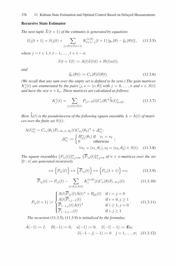
376 11 Kalman State Estimation and Optimal Control Based on Delayed Measurements
Recursive State Estimator
The next tuple X(t+ 1) of the estimates is generated by equations
x(j|t+ 1) = x(j|t) +∑
(ν,θ)∈S(t+1)
K(ν,θ)t+1−j(t+ 1) [yν(θ) − yν(θ|t)] , (11.3.5)
where j = t+ 1, t, t− 1, . . . , t+ 1− σ,
x(t+ 1|t) := A(t)x(t|t) +B(t)u(t),
andyν(θ|t) := Cν(θ)x(θ|t). (11.3.6)
(We recall that any sum over the empty set is defined to be zero.) The gain matricesKsj (t) are enumerated by the pairs [j, s = (ν, θ)] with j = 0, . . . , σ and s ∈ S(t)
and have the size n× kν . These matrices are calculated as follows:
Ksj (t) =
∑
(ν,θ)∈S(t)
Pj,t−θ(t)Cν(θ)T+
Λ(t)s(ν,θ). (11.3.7)
Here+
Λ(t) is the pseudoinverse of the following square ensemble Λ = Λ(t) of matri-ces over the finite set S(t):
Λ(t)s2s1 = Cν1(θ1)Pt−θ1,t−θ2(t)Cν2 (θ2)T +∆s2
s1 ;
∆s2s1 :=
Rν1χχ(θ1) if s1 = s20 otherwise
;
∀s1 = (ν1, θ1), s2 = (ν2, θ2) ∈ S(t). (11.3.8)
The square ensembles Pij(t)σi,j=0, P ij(t)σi,j=0 of n × n-matrices over the set[0 : σ] are generated recursively
7→
Pij(t)
7→
P ij(t)
7→
Pij(t+ 1)
7→; (11.3.9)
P ij(t) := Pij(t)−∑
(ν,θ)∈S(t)
K(ν,θ)i (t)Cν (θ)Pt−θ,j(t); (11.3.10)
Pij(t+ 1) :=
A(t)P ij(t)A(t) T +Rξξ(t) if i = j = 0
A(t)P i,j−1(t) if i = 0, j ≥ 1
P i−1,j(t)A(t) T if i ≥ 1, j = 0
P i−1,j−1(t) if i, j ≥ 1
. (11.3.11)
The recursion (11.3.5), (11.3.9) is initialized by the formulas:
A(−1) := I, B(−1) := 0, u(−1) := 0, x(−1| − 1) := Ea;
x(−1− j| − 1) := 0 j = 1, . . . , σ; (11.3.12)

11.3 State Estimator 377
Pij(0) =
0 if i ≥ 1 or j ≥ 1
Raa if i = j = 0. (11.3.13)
Note that in (11.3.5), (11.3.7), and (11.3.10), the sums are over the signals arrivedat the moment under consideration.
If no information is received at time t+ 1, the recursion step (11.3.5), (11.3.10)becomes much simpler:
P ij(t+ 1) = Pij(t+ 1), x(t+ 1|t+ 1) = A(t)x(t|t) +B(t)u(t);
x(j|t+ 1) = x(j|t) for j = t, t− 1, . . . , t+ 1− σ.Remark 11.3.2. Since the above estimator generates estimates of not only the currentbut also past states, it has points of similarity with the fixed-lag smoother [125,129].
11.3.3 The Major Properties of the State Estimator
Theorem 11.3.3. Suppose that Assumptions 11.2.1–11.2.4 hold. Then the above es-timator generates the sequence of minimum variance estimates; i.e.,
x(j|t) = E [x(j)|Y(t),S(t),U(t − 1)] (11.3.14)
whenever t − σ ≤ j ≤ t and j ≥ 0. Here Y(t), S(t), and U(t − 1) are defined by(11.2.4), and σ is the constant from Assumption 11.2.2.
The matrices Pij(t), P ij(t), i, j = 0, . . . , σ generated by the estimator are theconditional covariance matrices of the estimation errors
e(θ|s) := x(θ|s)− x(θ). (11.3.15)
More precisely, the following relations hold whenever t− i ≥ 0 and t− j ≥ 0:
P ij(t) := E[e(t− i|t)e(t− j|t) T
∣∣S(t)];
Pij(t) := E[e(t− i|t− 1)e(t− j|t− 1) T
∣∣S(t− 1)].
(11.3.16)
Furthermore, the estimation errors (11.3.15) do not depend on the control(11.2.5) (on p. 373).
The proof of this theorem and the remark to follow will be given in Sect. 11.7.The following remark presents useful technical facts.
Remark 11.3.4. (i) An access of the estimator to the quantity h(t) from (11.2.5) andmoreover, the knowledge of the entire sequences S(θ), 0 ≤ θ ≤ T and h(θ), 0 ≤θ ≤ T − 1 at any time t do not alter the minimum variance state estimate:
x(j|t) = E [x(j)|Y(t),S(t),U(t − 1)]
= E [x(j)|Y(t),S(t), h(0), . . . , h(t− 1)]
= E [x(j)|Y(t),S(T ), h(0), . . . , h(T − 1)] (11.3.17)
whenever t− σ ≤ j ≤ t and j ≥ 0.(ii) Given S(0), . . . , S(T ), h(0), . . . , h(T − 1), the estimation errors (11.3.15)
(where maxs−σ, 0 ≤ θ ≤ s) are independent of the observationsY (0), . . . , Y (s).

378 11 Kalman State Estimation and Optimal Control Based on Delayed Measurements
11.4 Stability of the State Estimator
The stability of the estimator is essential when estimation is performed over a longperiod of time. As is well known, the observation delays are the source of potentialinstability [93,97,209,210]. In this section, we show that the proposed state estimatoris stable provided natural assumptions hold. For the sake of conciseness, we confineourselves to the case when the system (11.2.1), (11.2.2) (but not the communicationchannels) is stationary.
We start with definitions required to state the assumptions under which the sta-bility issues will be addressed.
11.4.1 Almost Sure Observability via the Communication Channels
Definition 11.4.1. Consider the plant (11.2.1), (11.2.2) (on p. 372) with the noisesand control removed
x(t+ 1) = Ax(t), yν(t) = Cνx(t) ν = 1, . . . , l. (11.4.1)
This system is said to be observable via the communication channels on the interval[t0, t1] (for a given realization of the random delays τν(t)) if every state x(t0) canbe determined from the knowledge of the observations that are both dispatched andreceived within this interval.
Proposition 11.4.2. The system (11.4.1) is observable via the communication chan-nels on the interval [t0, t1] (for a given realization of the random delays τν(t)) ifand only if the following symmetric nonnegative n× n-matrix is positive-definite:
M(t0, t1) :=∑
(ν,θ):t0≤θ,θ+τν(θ)≤t1
(Aθ−t0
) TC TνCνA
θ−t0 . (11.4.2)
The proofs of the results formulated in this section will be given in Sect. 11.8.If a realization of τν(t) is not fixed, the matrix (11.4.2) is random.
Definition 11.4.3. Let an integer σ∗ = 0, 1, . . . exist such that M(t0, t1) > 0 almostsurely for some, possibly random, time instant t0 = t0(t1) ∈ [t1 − σ∗, t1] whenevert1 ≥ σ∗. Then the system (11.4.1) is said to be almost surely observable via thecommunication channels.
In fact, the matrix M(t0, t1) can be replaced here by the easier computable matrix
M(t0, t1) :=
t1∑
θ=t0
l∑
ν=1
αν(θ)(Aθ−t0
) TC TνCνA
θ−t0 ; (11.4.3)
αν(t) :=
0 if the signal yν(t) is lost, i.e., τν(t) =∞1 otherwise

11.4 Stability of the State Estimator 379
since M(t0, t1) ≤ M(t0, t1) ≤ M(t0, t1 + σ) due to Assumption 11.2.2. Thusverification of the above observability requires only the statistics of the data dropouts.It can be shown that whenever detA 6= 0, the system (11.4.1) is observable via thecommunication channels if and only if M(T − σ∗, T ) > 0 ∀T ≥ σ∗ almost surelyfor some σ∗ = 0, 1, . . .. Note that the random time instant t0 is not employed here.
Observability via the communication channels apparently implies that
The system (11.4.1) is observable in the standard sense.
In the remainder of this subsection we consider only such systems. Then the systemis clearly observable via the communication channels whenever they do not losesignals. To state other criteria, we say that a finite nonempty set
T ⊂(ν, t) : ν = 1, . . . , l, t = 0, 1, . . .
(11.4.4)
is representative for the system (11.4.1) if and only if
⋂
(ν,t)∈T
kerCνA(t−t−) = 0, where t− := mint : (ν, t) ∈ T. (11.4.5)
Proposition 11.4.4. The system (11.4.1) is observable via the communication chan-nels if and only if an integer σ∗ = 0, 1, . . . exists such that the set
T(T ) :=(ν, t) : T − σ∗ ≤ t ≤ T and the signal yν(t) is not lost
contains a representative subset almost surely for all T ≥ σ∗.Now we offer a number of facts concerning representative sets.
Proposition 11.4.5. Denote by O the collection of all matricesA such that the system(11.4.1) is observable in the standard sense. For almost all A ∈ O (with respect tothe Lebesgue measure), any finite set (11.4.4) such that the set Tν := t : (ν, t) ∈ Tcontains n elements (the νth sensor output is not lost n times) for all ν = 1, . . . , l isrepresentative.
By combining Propositions 11.4.4 and 11.4.5, we see that almost all observable (inthe standard sense) systems are observable via the communication channels with“low rates” of data dropout. The last property means that for some integer σ∗ > n,each channel does not lose (almost surely) at least n messages in every set of σ∗consecutively dispatched messages.
Proposition 11.4.6. Any finite set of the form
T = (ν, θ) : ν = 1, . . . , l, θ = t, t+ 1, . . . , t+ n− 1
(the channels lose no sensor signal dispatched within some time interval of durationn) is representative.

380 11 Kalman State Estimation and Optimal Control Based on Delayed Measurements
Thus an observable (in the standard sense) system is observable via the communi-cation channels if for some σ∗ > n, any time interval of duration σ∗ contains asubinterval of duration n − 1 such that all messages sent via the channels within itarrive (sooner or later) at the destination point. Note that this subinterval is commonfor all channels. The next proposition shows that if detA 6= 0, this subinterval maydepend on the channel.
Proposition 11.4.7. Suppose that detA 6= 0. Any finite set T such that the set Tν isan interval tν , tν + 1, . . . , tν + n − 1 of the length n (consequent n outputs of theνth sensor are not lost) for all ν = 1, . . . , l is representative.
Proposition 11.4.8. Let a(λ) := det(λI − A) be the characteristic polynomial ofthe matrix A. For t = 0, 1, . . ., we denote by pt(λ) the remainder of λt when dividedby a(λ). Suppose that for any ν = 1, . . . , l, the set Tν consists of n elements Tν =t1 < t2 < . . . < tn and the polynomials
pt1−t−(λ), pt2−t−(λ), . . . , ptn−t−(λ),
where t− is defined in (11.4.5), are linearly independent. Then the set T is represen-tative.
11.4.2 Conditions for Stability of the State Estimator
Now we suppose that the following three additional assumptions hold.
Assumption 11.4.9. The coefficients of the system (11.2.1), (11.2.2) (on p. 372) donot vary in course of time: A(t) ≡ A, Cν(t) ≡ Cν .
Assumption 11.4.10. The process disturbance in (11.2.1) and the noises in (11.2.2)are statistically stationary and nonsingular:
Rξξ(t) ≡ Rξξ > 0, Rνχχ(t) ≡ Rνχχ > 0.
Assumption 11.4.11. The system (11.4.1) is either almost surely observable via thecommunication channels (see Definition 11.4.1) or stable.
The following theorem is the main result of this section.
Theorem 11.4.12. Suppose that Assumptions 11.2.1– 11.2.4 (on pp. 373 and 374),and 11.4.9–11.4.11 hold. Then the state estimator described in Subsect. 11.3.2 (start-ing on p. 375) is a.s. uniformly exponentially stable; i.e.,
σ∑
j=0
‖e(t− j|t)‖ ≤ cρt−t0σ∑
j=0
‖e(t0 − j|t0)‖ (11.4.6)
whenever t ≥ t0. Here e(θ|t) are the errors (11.3.15) that occur provided the noisesare removed from (11.2.1) and (11.2.2) (on p. 372). The constants c > 0 and ρ ∈(0, 1) do not depend on t, t0 and the initial states of both the system and the estimator.

11.5 Finite Horizon Linear-Quadratic Gaussian Optimal Control Problem 381
It is tacitly assumed that the estimator gain matrices from (11.3.5) are calculated inthe presence of the noises for a specific initial data of the recursion (11.3.9) and fixed.
The proof of Theorem 11.4.12 will be given in Sect. 11.9.
Remark 11.4.13. Consider two initial random vectors a1 and a2 in (11.2.1). By(11.3.13), each of them ai gives rise to its own sequence of the estimator gain ma-
tricesi
Ksj(t). It follows from (11.4.6), along with (11.3.15), (11.3.16) and (11.3.7),
(11.3.8), that the discrepancy between these matrices is exponentially small∥∥∥∥
2
Ksj(t)−
1
Ksj(t)
∥∥∥∥ ≤ c∗(a1, a2)ρt∗ a.s.,
where ρ∗ ∈ (0, 1). Thus the influence of the initial state a on the proposed stateestimator vanishes in course of time.
11.5 Finite Horizon Linear-Quadratic Gaussian Optimal ControlProblem
Now we revert to the controlled system (11.2.1), (11.2.2) (on p. 372) and considerthe problem of minimizing the quadratic cost functional over a finite horizon
IT := E
T−1∑
t=0
[x(t + 1) TQ(t+ 1)x(t+ 1) + u(t) TΓ(t)u(t)] . (11.5.1)
Here Q(t + 1) ≥ 0 and Γ(t) > 0 are symmetric n × n and m × m matrices,respectively.
Now the observations are sent to not the observer but to the controller. In thisand the next sections, we consider the case where the control acts upon the plantimmediately and with no distortion. This means that in (11.2.5) (on p. 373), thevariable h(t) takes only one value and so can be dropped. Hence the natural class ofcontrol strategies is given by
u(t) = U [t,Y(t),S(t),U(t− 1)] , (11.5.2)
where U(·) is a deterministic function and Y(t),S(t),U(t−1) are defined in (11.2.3)and (11.2.4) (on p. 373). It should be remarked that by recursive excluding u(θ) fromthe right-hand side, (11.5.2) can be shaped into the form u(t) = Ψ [t,Y(t),S(t)]similar to (11.2.5).
In the other respects, the situation does not change. In particular, the measure-ment signals still incur random irregular delays and are sealed with time stamps.
To present the solution, we consider first the problem of minimizing the func-tional (11.5.1) subject to the constraints (11.2.1) in the case where the process dis-turbances are removed (ξ(t) ≡ 0) and the entire state x(t) is immediately accessibleby the controller. As is well known (see Appendix C), the solution of this simplifiedproblem is given by the linear feedback u(t) = −L(t)x(t), where

382 11 Kalman State Estimation and Optimal Control Based on Delayed Measurements
L(t) = F (t)−1B(t) T [Q(t+ 1) +H(t+ 1)]A(t); (11.5.3)
F (t) := Γ(t) +B(t) T [Q(t+ 1) +H(t+ 1)]B(t), (11.5.4)
and the symmetric n×n-matricesH(T ), H(T − 1), . . . , H(0) are calculated recur-sively in accordance with the following difference Ricatti equation:
H(t) = L(t) TΓ(t)L(t) +AL(t) T [Q(t+ 1) +H(t+ 1)]AL(t)
where AL(t) := A(t)−B(t)L(t). (11.5.5)
Here t = T − 1, T − 2, . . . , 0 and the recursion is initialized by putting H(T ) := 0.It is easy to see that H(t) ≥ 0 ∀t. So the matrix F (t)−1 in (11.5.3) does exist since
F (t) = Γ(t) +B(t) TQ(t+ 1)B(t) +B(t) TH(t+ 1)B(t) ≥ Γ(t) > 0. (11.5.6)
Now we are in a position to state the main result of the section.
Theorem 11.5.1. Suppose that Assumptions 11.2.1 and 11.2.2 (on p. 374) hold. Thenthe optimal strategy (11.5.2) exists and is given by the formula
u(t) = −L(t)x(t|t) for t = 0, 1, . . . , T − 1. (11.5.7)
Here the gain matrices L(t) are determined by (11.5.3)–(11.5.5), and x(t|t) is theestimation of the current state x(t) generated by the estimator from Subsect. 11.3.2.
Now this estimator should be implemented at the controller site.The proof of Theorem 11.5.1 will be given in Sect. 11.7.
11.6 Infinite Horizon Linear-Quadratic Gaussian OptimalControl Problem
In this section, we consider the infinite-horizon time-invariant system (11.2.1),(11.2.2) and deal with the problem of minimizing the average cost per unit time
limT→∞
T−1IT . (11.6.1)
Here IT is defined by (11.5.1). Apart from Assumptions 11.2.1 and 11.2.2 (onp. 374), several additional assumptions are adopted. The first of them extends As-sumption 11.4.9 (on p. 380).
Assumption 11.6.1. The coefficients of both the system (11.2.1), (11.2.2) (on p. 372)and the functional (11.5.1) (on p. 381) do not vary as time progresses:
A(t) ≡ A, B(t) ≡ B, Cν(t) ≡ Cν , Q(t) ≡ Q, Γ(t) ≡ Γ.
Assumption 11.6.2. The pairs (A,B) and (A,Q) are stabilizable and detectable,respectively.

11.6 Infinite Horizon Linear-Quadratic Gaussian Optimal Control Problem 383
The next assumption relaxes Assumption 11.4.10 (on p. 380) by dropping the re-quirement that the noises should be nonsingular.
Assumption 11.6.3. The noises in (11.2.1) and (11.2.2) are statistically stationary:
Rξξ(t) ≡ Rξξ, Rνχχ(t) ≡ Rνχχ.
Assumption 11.6.4. A constant p ∈ (0,+∞) exists such that
E tr [P00(t)− P 00(t)] ≤ p ∀t = 0, 1, 2, . . . . (11.6.2)
Here Pij(t), P ij(t) are the symmetric n × n matrices generated by the estimatorfrom Subsect. 11.3.2 (starting on p. 375).
It should be remarked that the matrices Pij(t), P ij(t) are generated by formulas(11.3.7)–(11.3.11), (11.3.13), which do not employ controls. So they are well definedin the current situation, where the controls have not been specified yet.
An informal interpretation of Assumption 11.6.4 proceeds from the fact that by(11.3.14), (11.3.15), and (11.3.16), P00(t) and P 00(t) are the covariance matricesof the current state estimation errors that occur, respectively, before and after thearrival of the current observation message. So the quantity E tr [P00(t) − P 00(t)]from (11.6.2) evaluates to what extent this message improves the accuracy of theestimate. In view of this, we call this quantity the efficiency of the tth message. ThusAssumption 11.6.4 means that there is no observation message with arbitrarily highefficiency.
A criterion for Assumption 11.6.4 to hold will be offered at the end of this sec-tion.
Now we consider the algebraic Ricatti equation
H = L THΓLH + (A−BLH) T(Q+H)(A−BLH) (11.6.3)
with respect to the unknown n× n symmetric matrix H . Here
LH := F−1H B T(Q+H)A, FH := Γ +B T(Q+H)B. (11.6.4)
Under the circumstances, this equation is well known to have a solutionH for whichthe matrix
AH := A−BLH (11.6.5)
is asymptotically stable:
‖(AH)t‖ ≤ cρt t = 0, 1, 2, . . . (11.6.6)
for some c > 0, ρ ∈ (0, 1). This solution is unique and nonnegative. In particular,the last property implies that the inverse matrix F−1
H in (11.6.4) does exist.Now we are in a position to state the main result of the section.

384 11 Kalman State Estimation and Optimal Control Based on Delayed Measurements
Theorem 11.6.5. Suppose that Assumptions 11.2.1, 11.2.2 and 11.6.1–11.6.4 (onpp. 373 and 382) hold. Then the feedback
u(t) = −LH x(t|t) (11.6.7)
furnishes the minimum of the average cost for unit time (11.6.1) over all controlstrategies (11.5.2). In (11.6.7), the estimate x(t|t) is generated by the state estimatorfrom Subsect. 11.3.2 (starting on p. 375).
The proof of this theorem will be given in Sect. 11.10.As will be shown in Sect. 11.10 (for details, see Lemma 11.10.1 on p. 397), the
stationary control gain (11.6.7) can be viewed as the limit of the optimal nonstation-ary gain (11.5.7). At the same time, both gains are fed by the state estimate producedby the common and nonstationary estimation algorithm.
We close the section with sufficient conditions for Assumption 11.6.4 to hold andthe control strategy (11.6.7) to stabilize the system.
Proposition 11.6.6. Suppose that Assumptions 11.2.1, 11.2.2 and 11.6.1–11.6.3 (onpp. 373 and 382) are true. Assumption 11.6.4 (on p. 383) holds, and the controlstrategy (11.6.7) stabilizes the system
supt=0,1,...
E‖x(t)‖2 <∞
whenever at least one of the following claims is true:
(i) The uncontrolled plant (11.2.1), (11.2.2) (on p. 372) is asymptotically stable:‖At‖ ≤ γµt for t = 0, 1, 2, . . . and some γ > 0, µ ∈ (0, 1);
(ii) This plant is almost surely observable via the communication channels.1
The proof of this proposition will be given in Sect. 11.10.
11.7 Proofs of Theorems 11.3.3 and 11.5.1 and Remark 11.3.4
Proof of Theorem 11.3.3 and Remark 11.3.4 (on p. 377). Consider the linear space
Z :=Z = zν,jlν=1
σj=0 : zν,j ∈ R
kν ∀ν, j.
We recall that l is the number of sensors, kν is the dimension of the νth sensor output,and σ is taken from Assumption 11.2.2 (on p. 374). We also set
x(−σ) := x(−σ + 1) := · · · := x(−1) := 0
and introduce the vectors
1See Definition 11.4.3 on p. 378.

11.7 Proofs of Theorems 11.3.3 and 11.5.1 and Remark 11.3.4 385
X(t) := col[x(t), x(t − 1), . . . , x(t− σ)
];
Z(t) :=zν,j∈ Z, where zν,j :=
yν(t− j) if (ν, t− j) ∈ S(t)0 otherwise
.
(11.7.1)
The vector Z(t) can be interpreted as composed of the currently arrived observationsY (t) from (11.2.3) (on p. 373) supplemented with several zeros. In terms of X(t)and Z(t), relations (11.2.1) and (11.2.2) (on p. 372) take the forms, respectively:
X(t+ 1) = A(t)X(t) + B(t)u(t) + E ξ(t) t = 0, . . . , T − 1; (11.7.2)
X(0) = a := col (a, 0, . . . , 0); (11.7.3)
Z(t) = C[t, S(t)
]X(t) + Ξ
[t, S(t)
]t = 0, . . . , T. (11.7.4)
Here
A(t) :=
A(t) 0 0 · · · 0 0I 0 0 · · · 0 00 I 0 · · · 0 00 0 I · · · 0 0· · · · · · · ·· · · · · · · ·0 0 0 · · · I 0
andE := col
[I, 0, . . . , 0
]
B(t) := col[B(t), 0, . . . , 0
] .
(11.7.5)Furthermore for any t ≤ T , S ⊂ (ν, j) : ν = 1, . . . , l, j = 0, . . . , σ, and X =col (x0, x1, . . . , xσ) ∈ R(σ+1)n, the following relations hold:
C[t, S]X := zν,jlν=1σj=0 ∈ Z,
where zν,j :=
Cν(t− j)xj if (ν, t− j) ∈ S0 otherwise
; (11.7.6)
Ξ[t, S] := ζν,jlν=1σj=0 ∈ Z,
where ζν,j :=
χν(t− j) if (ν, t− j) ∈ S0 otherwise
. (11.7.7)
Formula (11.2.5) (on p. 373) shapes into
u(t) = U [t, Z(0), . . . , Z(t), S(0), . . . , S(t), h(t)] .
By Assumptions 11.2.2 and 11.2.4 (on p. 374), the quantities τν(t) and h(t)are independent of a, ξ(t), and χν(t). So evidently are the random sets S(t)defined by (11.2.3) (on p. 373). Then (11.2.7) (on p. 374) implies that the vectorsa, ξ(t), and Ξ[t, S(t)] conditioned over
S(0), . . . , S(T ), h(0), . . . , h(T − 1) (11.7.8)

386 11 Kalman State Estimation and Optimal Control Based on Delayed Measurements
are (singular) Gaussian and independent. This yields that conditioning all randomvectors over (11.7.8) reduces the system to that considered in the classic Kalmanfiltering theory. This theory gives the expression for the minimum variance estimateX(t|t) ofX(t) based onZ(0), . . . , Z(t), and due to the preliminary conditioning, thequantities from (11.7.8). This estimate is generated recursively by the correspondingKalman filter so that only the sets S(0), . . . , S(t) from (11.7.4) and u(0), . . . , u(t−1) are required to compute X(t|t). This implies (i) of Remark 11.3.4 (on p. 377) andmeans that X(t|t) is in fact the minimum variance estimate of X(t) based on
Z(0), . . . , Z(t), S(0), . . . , S(t), and u(0), . . . , u(t− 1).
Theorem 11.3.3 (on p. 377) results from putting (11.7.5)–(11.7.7) into the equa-tions giving the solution of the classic minimum variance estimation problem; i.e.,formulas (C.8)–(C.13) (on pp. 510 and 511), along with elementary transformationsof the resultant formulas. This also gives the last claim of Theorem 11.3.3 and (ii) ofRemark 11.3.4 (on p. 377) thanks to (ii)–(iv) of Theorem C.2 (on p. 511).
Proof of Theorem 11.5.1 (on p. 382). In terms of the vectors (11.7.1), the problemunder consideration takes the form:
minimize E
T−1∑
t=0
[X(t+ 1) TQ(t+ 1)X(t+ 1) + u(t) TΓ(t)u(t)] ; (11.7.9)
where Q(t) :=
Q(t) 0 · · · 00 0 · · · 00 0 · · · 0· · · · · ·0 0 · · · 0
, (11.7.10)
subject to the constraints (11.7.2)–(11.7.4) and
u(t) = U [t, Z(0), . . . , Z(t), S(0), S(1), . . . , S(t), u(0), . . . , u(t− 1)] . (11.7.11)
Now in (11.7.8), h(t) take only one value and so may be ignored. As was shown, thevectors a, ξ(t), andΞ[t, S(t)] conditioned overS(0), . . . , S(T−1) are Gaussian andindependent. This yields that the problem resulting from (11.7.2)–(11.7.4), (11.7.9),and (11.7.11) by expanding the class of admissible controls as follows:
u(t) = U [t, Z(0), . . . , Z(t), S(0), . . . , S(T − 1), u(0), . . . , u(t− 1)]
reduces to a particular case of the standard LQG optimal control problem (see Ap-pendix C starting on p. 509). By Theorem C.5 (on p. 513) from this appendix, thesolution of the latter problem is given by the linear feedback u(t) = −F(t)X(t)that is optimal for the problem of minimizing the functional (11.7.9) subject to theconstraints (11.7.2) and (11.7.3) in the case where ξ(t) ≡ 0 and the entire state X ismeasured. This controller is fed by the minimum variance estimate X(t|t) of X(t)based on the observationsZ(0), . . . , Z(t) and the known controls u(0), . . . , u(t−1).

11.8 Proofs of the Propositions from Subsect. 11.4.1 387
This estimate is generated recursively by the Kalman filter so that only the setsS(0), . . . , S(t) from (11.7.4) are in fact required to compute X(t|t). Calculating thegain matrix F(t) employs the coefficients of the functional (11.7.9) and the equation(11.7.2) for the time instants t, t + 1, . . . , T . Since these coefficients do not dependon the sets S(0), . . . , S(T − 1) and are known in advance, the control appears tobe of the form (11.7.11). So it furnishes the optimum over the strategies given by(11.7.11).
Theorem 11.5.1 (on p. 382) results from putting the expressions (11.7.5)–(11.7.7)and (11.7.10) into the equations giving the solutions of the minimum variance stateestimate and the standard LQG control problems, respectively (i.e., formulas (C.8)–(C.13) and (C.18)–(C.21) on pp. 510–512 from Appendix C), along with elementarytransformations of the resultant formulas.
11.8 Proofs of the Propositions from Subsect. 11.4.1
Proof of Proposition 11.4.2 (on p. 378). Given two processes
pi =([xi(t)]
t1t=t0 , [Yi(t)]
t1t=t0
), i = 1, 2
in the system (11.4.1) (here Yi(t) is given by (11.2.3) (on p. 373), where S(t) isreplaced by S(t) := (ν, θ) ∈ S(t) : θ ≥ t0), we have thanks to (11.2.3), (11.4.1),and (11.4.2),
[x2(t0)− x1(t0)]T
M(t0, t1)[x2(t0)− x1(t0)] =
t1∑
t=t0
‖Y2(t)− Y1(t)‖2.
So(Y1(t) = Y2(t)∀t = t0, . . . , t1
)⇒ p1 = p2 if and only if M(t0, t1) > 0. ⊓⊔
Proof of Proposition 11.4.4 (on p. 379). Note first that whenever t0 ≥ t1 − σ∗,(11.4.3) (on p. 378) yields
z TM(t0, t1)z =∑
(ν,θ)∈T(t1):θ≥t0
∥∥CνAθ−t0z∥∥2. (11.8.1)
If T(t1) contains a representative subset T, then putting here t0 := t− the constantt− from (11.4.5) (on p. 379) makes the sufficiency part of the proposition apparent.
Conversely, let the system (11.4.1) be observable via the communication chan-nels; i.e., there is σ∗ ≥ 0 such that M(t0, t1) > 0 for some t0 ∈ [t1 − σ∗, t1] almostsurely. Then (11.8.1) implies that the set T := (ν, θ) ∈ T(t1) : θ ≥ t0 is represen-tative since t0 < t− ⇒ detA 6= 0. ⊓⊔
Proposition 11.4.6 (on p. 379) is evident.Proof of Proposition 11.4.8 (on p. 380). By the definition of p t(λ),
λt = bt(λ)a(λ) + p t(λ), (11.8.2)

388 11 Kalman State Estimation and Optimal Control Based on Delayed Measurements
where bt(λ) is a polynomial. Thanks to the assumptions of the proposition, p s1(λ),. . . , p sn(λ) (where si := ti − t−) is the basis in the space of all polynomials ofdegree≤ n− 1. So for j = 0, . . . , n− 1,
λj =
n∑
i=1
γ(j)i p si(λ) =
n∑
i=1
γ(j)i λsi −
[n∑
i=1
γ(j)i bsi(λ)
]a(λ)
for some γ(j)i ∈ R. Since a(A) = 0, we get
CνAj =
n∑
i=1
γ(j)i CνA
ti−t− ,⋂
t∈Tν
kerCνAt−t− =
n⋂
i=1
kerCνAti−t−
⊂n−1⋂
j=0
kerCνAj ,
⋂
(ν,t)∈T
kerCνAt−t− ⊂
n−1⋂
j=0
l⋂
ν=0
kerCνAj = 0. ⊓⊔
Proof of Proposition 11.4.7 (on p. 380). Pick ν = 1, . . . , l. Suppose that
n−1∑
j=0
γjp tν+j−t−(λ) ≡ 0
for some γj ∈ R, and denote γ(λ) := γ0 + γ1λ+ · · · γn−1λn−1. Then by (11.8.2)
γ(λ)λtν−t− =
n−1∑
j=0
γjbtν+j−t−(λ)
a(λ).
Since a(0) 6= 0, the polynomials a(λ) and λtν−t− are coprime. So the polynomiala(λ) of degree n must divide the polynomial γ(λ) of degree≤ n−1. Hence γ(λ) ≡0, γ0 = · · · = γn−1 = 0; i.e., the polynomials p tν−t−(λ), . . . , p tν+n−1−t−(λ) arelinearly independent. Proposition 11.4.8 completes the proof. ⊓⊔
Proof of Proposition 11.4.5 (on p. 379). Since
P(A) := det
l∑
ν=1
n−1∑
j=0
AjCνCTν (A T)
j
is evidently a nonzero polynomial in the entries of the matrix A, and O = A :P(A) 6= 0, the set O is of full Lebesgue measure in the space of all n× n matricesA. Now let a tuple t = t1, . . . , tn of integers ti ≥ 0, ti 6= tj ∀ i 6= j be given. It iseasy to see that for any t = 0, 1, . . ., the coefficients of the polynomial
p t(λ) = p t(0) + · · ·+ p t(n− 1)λn−1
from Proposition 11.4.8 (on p. 380) are polynomials in the entries of A. So is
pt(A) := det
(p t1 (0) ... p t1 (n−1)... ... ...
p tn (0) ... p tn (n−1)
).

11.9 Proof of Theorem 11.4.12 389
Note that pt(A) 6≡ 0. Indeed, otherwise, any polynomial a(λ) = λn + · · · of degreen would divide some nonzero polynomial of the form γ1λ
t1 + · · ·+ γnλtn . In terms
of the roots λ1, . . . , λn of a(λ), this implies
q(λ1, . . . , λn) := det
(λ
t11 ... λt1
n... ... ...λtn1 ... λtn
n
)= 0.
This relation holds at least for all real λi. At the same time,
q(λ1, . . . , λn) =∑
α
(−1)inv(α)λtα(1)
1 · · ·λtα(n)n
(the sum is over all permutations α = [α(1), . . . , α(n)] of 1, 2, . . . , n andinv(α) is the number of inversions in the permutation) a nonzero polynomial andso q(λ1, . . . , λn) 6= 0 for some real λi. The contradiction obtained proves thatpt(A) 6≡ 0. Hence the set Rt := A ∈ O : pt(A) 6= 0 is of full measure. So isthe set R :=
⋂t Rt.
Now let A ∈ R. It is easy to see that any set T with the properties describedin Proposition 11.4.5 (on p. 379) satisfies the hypotheses of Proposition 11.4.8 (onp. 380), which completes the proof. ⊓⊔
11.9 Proof of Theorem 11.4.12 on p. 380
The state estimator introduced in Subsect. 11.3.2 (starting on p. 375) is in fact theconventional Kalman filter related to the representation of the system in the aug-mented form (11.7.2)–(11.7.4) (on p. 385). However in the vast literature on theKalman filter, the authors failed to find a reference that proves Theorem 11.4.12. Thereason is that the nonstationary (in the sensor part) system (11.7.2), (11.7.4) loses ob-servability due to the state augmentation. In the case of unstable but observable inthe sense of Assumption 11.4.11 (on p. 380) system (11.4.1), this causes violationof assumptions under which the stability of the Kalman filter was established in thestudies known to the authors. In view of this, we adduce an independent proof. Itemploys a slightly refined standard technique.
From now on, Assumptions 11.2.1–11.2.4 (on pp. 373 and 374), and 11.4.9–11.4.11 (on p. 380) are supposed to hold. Introduce the following vector and matri-ces:
E(t) :=
e(t|t)...
e(t− σ|t)
, P(t) :=
P00(t) · · ·P0σ(t)
...Pσ0(t) · · ·Pσσ(t)
,
P(t) :=
P 00(t) · · ·P 0σ(t)
...P σ0(t) · · ·Pσσ(t)
. (11.9.1)

390 11 Kalman State Estimation and Optimal Control Based on Delayed Measurements
Here e(θ|t) are the estimation errors (11.3.15) (on p. 377), Pij(t), P ij(t) are thematrices generated by the estimator, and σ is taken from Assumption 11.2.2 (onp. 374). By Theorem 11.3.3 (on p. 377) and (11.3.7)–(11.3.11), (11.3.13) (on p. 376),these errors and matrices do not depend on the control (11.2.5) (on p. 373). Forsimplicity, we assume that u(t) ≡ 0. In the remainder of the section, “constant”means “deterministic constant.”
Lemma 11.9.1. Constants β > 0, β > 0 exist such that P(t) ≤ βI and P(t) ≤ βIalmost surely for all t.
Proof. Suppose that the first case from Assumption 11.4.11 (on p. 380) holds; i.e.,the system (11.4.1) (on p. 378) is almost surely observable via the communicationchannels.2 In view of (11.2.3) (on p. 373) and (11.4.2) (on p. 378), one can supposethat in Definition 11.4.3, t0(t1) is a deterministic function of t1, S(0), . . . , S(t1).Furthermore, the matrixM [t0(t1), t1] is determined by the sample sequence assumedby τν(t) over the time interval [t0(t1), t1] of a bounded duration t1 − t0(t1) ≤ σ∗.There are no more than finitely many such sample sequences (up to the change ofthe variable t 7→ t− t0(t1)) even if t1 is not fixed. This implies that for some µ > 0,
∥∥M [t0(t1), t1]−1∥∥ ≤ µ a.s. whenever t1 ≥ σ∗. (11.9.2)
Choose t1 ≥ σ∗ and denote
t0 := t0(t1), S(t0, t1) := (ν, θ) : t0 ≤ θ, θ + τν(θ) ≤ t1.
By (11.2.1) and (11.2.2) (on p. 372),
x(t) = At−t0x(t0) +
t−1∑
p=t0
At−1−pξ(p) whenever t > t0; (11.9.3)
yν(t) = CνAt−t0x(t0) + Cν
t−1∑
p=t0
At−1−pξ(p) + χν(t) whenever t ≥ t0;
∑
(ν,θ)∈S(t0,t1)
(A T)θ−t0 C Tν yν(θ) =
∑
(ν,θ)∈S(t0,t1)
(A T)θ−t0C TνCνA
θ−t0
︸ ︷︷ ︸M(t0,t1)
x(t0)
+∑
(ν,θ)∈S(t0,t1)
(A T)θ−t0C Tν
Cν
θ−1∑
j=t0
Aθ−1−jξ(j) + χν(θ)
. (11.9.4)
Put s := t1 +σ+1 and for j = 0, . . . , σ, consider the following estimate of x(s−j):
x(s− j) := As−j−t0M(t0, t1)−1
∑
(ν,θ)∈S(t0,t1)
(A T)θ−t0C Tν yν(θ).
2See Definition 11.4.3 on p. 378.

11.9 Proof of Theorem 11.4.12 391
Now we invoke the notation S(s − 1) from (11.2.4) (on p. 373). Then (11.3.14)–(11.3.16) (on p. 377) imply
trPjj(s) = E[‖e(s− j|s− 1)‖2
∣∣S(s− 1)]
≤ E[‖x(s− j)− x(s− j)‖2|S(s− 1)
]. (11.9.5)
We recall that the symbol tr stands for the trace of a matrix. By (11.9.3) and (11.9.4),
x(s− j)− x(s− j) =
s−1−j∑
i=t0
As−1−i−jξ(i)
−As−t0−jM(t0, t1)−1
∑
(ν,θ)∈S(t0,t1)
(A T)θ−t0C Tν
Cν
θ−1∑
j=t0
Aθ−1−jξ(j) + χν(θ)
.
We note that t1 − t0 = t1 − t0(t1) ≤ σ∗ by Definition 11.4.3 (on p. 378), and wedenote
a := max‖At‖ : t = 0, . . . , σ∗ + σ + 1, c := max‖Cν‖ : ν = 1, . . . , l.Then in view of (11.9.2),
1/2E[‖x(s− j)− x(s− j)‖2|S(s− 1)
]≤ [σ∗ + σ]a2 trRξξ
+ a4µ2c2σ∗l[c2a2σ2
∗l trRξξ + maxν=1,...,l
trRνχχ].
Here s = t1 + σ + 1 and t1 ≥ σ∗ is arbitrary. Thus trPjj(t) is bounded above. Tocomplete the proof, we note that P jj(t) ≤ Pjj(t) thanks to (11.3.16) (on p. 377) andemploy (11.9.1).
Now suppose that the second case from Assumption 11.4.11 (on p. 380) holds;i.e., the system (11.4.1) (on p. 378) is stable. By taking x(s′) := 0 ∀s′ in (11.9.5)and invoking Assumption 11.2.2 (on p. 374), we see that trPjj(t) is still boundedabove. After this, the proof is completed as in the previous case. ⊓⊔
From now on, we consider the vectors E(t) given by (11.9.1) in the case wherethe noises are removed from the plant equations (11.2.1) and (11.2.2) (on p. 372).
Lemma 11.9.2. Constants α, α, β, β > 0, and t∗ exist such that for t ≥ t∗,αI ≤ P(t) ≤ βI, αI ≤ P(t) ≤ βI a.s.; (11.9.6)
E(t+ 1) = AE(t) + V (t+ 1) a.s.,
where V (t+ 1) :=[P(t+ 1)P(t+ 1)−1 − I
]AE(t); (11.9.7)
E(t) TP(t)−1E(t)− E(t − 1) TP(t− 1)−1E(t− 1) ≤ −V (t) TP(t)−1V (t)
−∑
(ν,θ)∈S(t)
e(θ|t) TC Tν
[Rνχχ
]−1
Cνe(θ|t) a.s. (11.9.8)

392 11 Kalman State Estimation and Optimal Control Based on Delayed Measurements
Proof. The upper bounds from (11.9.6) are established by Lemma 11.9.1. To obtainthe lower ones, let us fix a realization of τν(t) by conditioning all random quantitiesover τν(t). It follows from (11.3.14)–(11.3.16) (on p. 377) and (11.9.1) that the errorcovariance matrices are no less P(t) ≥ P f (t),P(t) ≥ P f (t) than those in the casewhere the observations are received without losses and delays; i.e., S(t) = (ν, t) :ν = 1, . . . , l. Then with regard to Assumptions 11.2.1 and 11.4.10 (on pp. 373 and380) and well-known facts about the asymptotic behaviour of the classic Kalmanfilter [123, p.100] applied to the augmented system, we conclude that the matricesP f (t) and P f (t) are bounded from below by constant positive-definite matrices forlarge t. This completes the proof of (11.9.6).
Relations (11.9.7) and (11.9.8) are immediate from, e.g., (54)–(56) and (58) [43].It was assumed in [43] that the noise Ξ in (11.7.4) (on p. 385) is nonsingular, and thematrix A in (11.7.2) is invertable. The first requirement can be met by substitutingχν(t) in place of zeros in (11.7.7) (on p. 385). Here χν(t) ∈ Rkν are Gaussian mu-tually independent and independent of τν(t), ξ(t), χν (t) zero-mean random vectorswith Eχν(t)χν(t)
T = I . It is easy to check that this does not alter the Kalman filterformulas. The invertability of A was employed in (57) [43] to ensure that
D ≥ 0 & P > 0 & APA T +D > 0 ⇒ A T[APA T +D]−1A ≤ P−1.
However this implication holds for any matrix A, which can be proved by consider-ing a nonsingular perturbation Aε, detAε 6= 0,Aε → A as ε → 0 of A and lettingε→ 0 in the above inequality. ⊓⊔
By (11.9.6) and (11.9.8),
β −1‖E‖2 ≤W (t,E) := E TP(t)−1E ≤ α−1‖E‖2 a.s. whenever t ≥ t∗,(11.9.9)
W [t+ 1,E(t+ 1)] ≤W [t,E(t)] a.s. whenever t ≥ t∗. (11.9.10)
This implies that the state estimator is Lyapunov stable. The following lemma showsthat the additional estimate
λW [t+ r,E(t + r)] ≤W [t,E(t)] a.s. whenever t ≥ t (11.9.11)
implies the exponential stability. Here λ > 1, t = t∗, t∗+1, . . ., and r = 1, 2, . . . areconstants.
(on p. 380) is true.
Proof. By (11.9.6) and (11.9.7),
‖E(t+ 1)‖ ≤ βα−1‖A‖‖E(t)‖ a.s.
whenever t ≥ t∗. For t ≤ t∗, (11.2.1), (11.2.2), and (11.3.5)–(11.3.11) (on pp. 372,376) yield E(t + 1) = R(t)E(t), where R(t) = R[t, S(0), . . . , S(t + 1)] and R isa deterministic function. The random sequence S(0), . . . , S(t∗ + 1) assumes only
Lemma 11.9.3. Suppose that (11.9.11) holds. Then the conclusion of Theorem 11.4.12

11.9 Proof of Theorem 11.4.12 393
finitely many samples. Hence ‖R(t)‖ ≤ f ∀t = 0, . . . , t∗ a.s. for some constant f .By the foregoing, there is µ > 1 such that
‖E(t2)‖ ≤ µt2−t1‖E(t1)‖ a.s. whenever t2 ≥ t1. (11.9.12)
Thanks to (11.9.10), (11.9.11), λW [t,E(t)] ≤ W [θ,E(θ)] a.s. whenever t − r ≥θ := maxt0, t. Then invoking (11.9.9) gives
‖E(t)‖ ≤√βα−1λ−j/2‖E(θ)‖ a.s. whenever t− jr ≥ θ = maxt0, t.
Now let t ≥ t0. By employing the above inequality with j ≥ r−1(t− θ)− 1 if t ≥ tand (11.9.12) otherwise, and putting κ :=
√βα−1λ, ρ := λ−r
−1/2 < 1, we get
‖E(t)‖ ≤
κρt−θ‖E(t0)‖ if t0 ≥ t,‖E(t )‖
(11.9.12)≤ µbt−t0‖E(t0)‖ if t0 < t,
and t ≥ t,
µt−t0‖E(t0)‖ if t < t
≤
κ if t0 ≥ t and t ≥ t,κρt0−btµbt if t0 < t and t ≥ t,µbtρt0−bt if t < t
ρt−t0‖E(t0)‖.
This clearly implies (11.4.6) (on p. 380) with a properly chosen constant c. ⊓⊔
The remainder of the section is devoted to proving (11.9.11). In so doing, thefollowing fact will play a key role.
Lemma 11.9.4. Deterministic sequences κ(i)∞i=0, d(i)∞i=0 ⊂ (0,∞) exist suchthat
W [t+ k,E(t+ k)] ≤ κ(k)‖e(t|t)‖2 + d(k)
t+k∑
j=t+1
V (j) TP(j)−1V (j) (11.9.13)
a.s. whenever k ≥ σ and t ≥ t∗. If the system (11.4.1) (on p. 378) is stable, thesesequences can be chosen so that
κ(k)→ 0 as k →∞ and d := supkd(k) <∞. (11.9.14)
Proof. Owing to (11.9.7) and (11.9.9),
E(t+ k) = AkE(t) +
t+k∑
j=t+1
At+k−jV (j);
αW [t+ k,E(t+ k)] ≤ ‖E(t+ k)‖2 ≤ 2‖AkE(t)‖2 + 2
k−1∑
i=0
∥∥Ai∥∥2
t+k∑
j=t+1
‖V (j)‖2.

394 11 Kalman State Estimation and Optimal Control Based on Delayed Measurements
Here ‖V (j)‖2 ≤ βV (j) TP(j)−1V (j) by (11.9.6), and due to (11.7.5) (on p. 385),
Ak =
(Ak 0···0...
...Ak−σ 0···0
).
So ‖AkE(t)‖ ≤ ‖Ak‖‖e(t|t)‖ thanks to (11.9.1). Thus (11.9.13) does hold with
κ(k) := 2α−1∥∥Ak
∥∥2, d(k) := 2α−1β
k−1∑
i=0
∥∥Ai∥∥2. (11.9.15)
If the system (11.4.1) (on p. 378) is stable, so evidently is (11.7.2) (on p. 385). Then(11.9.14) is immediate from (11.9.15). ⊓⊔
Proof of (11.9.11) in the case of stable system (11.4.1). Pick t ≥ t∗ + 1 andk ≥ σ. By neglecting the last summand on the right in (11.9.8) and summing theresultant inequalities over t = t, . . . , t+ k, we get
W [t+ k,E(t+ k)] +
t+k∑
t=t
V (t) TP(t)−1V (t) ≤W [t− 1,E(t− 1)]
a.s. Here thanks to (11.9.13) and (11.9.14),
t+k∑
t=t
V (t) TP(t)−1V (t) ≥ d−1 W [t+ k,E(t+ k)]− κ(k)‖e(t− 1|t− 1)‖2
a.s. Furthermore, due to (11.9.1) and (11.9.9),
‖e(t− 1‖t− 1)‖2 ≤∥∥E(t− 1)
∥∥2 ≤ βW [t− 1,E(t− 1)] a.s.
Thusλ(k)W [t+ k,E(t+ k)] ≤W [t− 1,E(t− 1)] a.s.,
where
λ(k) := (1 + d−1)[1 + d−1βκ(k)]→ 1 + d−1 > 1 as k →∞
by (11.9.14). Picking k such that λ(k) > 1 yields (11.9.11) with r := k + 1.
In the case where the system (11.4.1) is not stable, we need more preliminaries.
Lemma 11.9.5. Suppose that Q1(z) and Q2(z) are nonnegative quadratic forms inz ∈ Rp, and Q2(z) = 0 whenever Q1(z) = 0. A constant γ > 0 exists such that
Q1(z) ≥ γQ2(z) ∀z.

11.9 Proof of Theorem 11.4.12 395
Proof. For i = 1, 2, introduce the symmetric p × p matrix Ωi related to Qi(z) =z TΩiz, and denote by π the orthogonal projection onto L := (kerΩ1)
⊥. SinceQi(z) = 0⇔ Ωiz = 0, then z − πz ∈ kerΩ1 ⊂ kerΩ2 ∀z. So
Qi(z) = [(z − πz) + πz] TΩi[(z − πz) + πz] = (πz) TΩi(πz) = Qi(πz).
The form Q1(z) is positive-definite on L and hence Q1(z) ≥ γQ2(z) ∀z ∈ L forsome γ > 0. Thus Q1(z) = Q1(πz) ≥ γQ2(πz) = γQ2(z) ∀z. ⊓⊔
Lemma 11.9.6. A constant γ > 0 exists such that
It :=t+σ∑
t=t0(t)
1
2V (t) TP(t)−1V (t) +
∑
(ν,θ)∈S(t)
e(θ|t) TC Tν
[Rνχχ
]−1Cνe(θ|t)
≥ γ∥∥e[t0(t)|t0(t)
]∥∥2a.s. ∀t ≥ t∗ + σ∗ + 1. (11.9.16)
Here σ∗, t0(t), and t∗ are the time instants from Definition 11.4.3 (on p. 378) andLemma 11.9.2.
Proof. In view of (11.9.6) and the inequality t− t0(t) ≤ σ∗ from Definition 11.4.3,V TP(t)−1V ≥ β−1‖V ‖2 in (11.9.16). Furthermore χ T[Rνχχ]−1χ ≥ υ−1‖χ‖2,
where υ := maxν ‖Rνχχ‖. Hence It is no less than the minimum value of the costfunctional in the following optimization problem:
minimize1
2β
t∑
t=t0(t)+1
‖V (t)‖2+υ−1t∑
t=t0(t)
∑
(ν,θ)∈S(t):θ≥t0(t)εt−θ(t)
TC TνCνεt−θ(t)
subject to
E(t) = col[ε0(t), . . . , εσ(t)
]= AE(t− 1) + V (t), t = t0(t) + 1, . . . , t
and E[t0(t)] = E[t0(t)]. The change of the variable t 7→ t− t0(t) shapes it into
minimize I :=1
2β
k∑
t=1
‖V (t)‖2+υ−1k∑
t=0
∑
(ν,θ):θ≥0,
[ν,θ+t0(t)]∈S[t+t0(t)]
εt−θ(t)TC T
νCνεt−θ(t)
subject to
E(t) = AE(t− 1) + V (t), t = 1, . . . , k, E(0) = Z.
Here k := t−t0(t) ≤ σ∗ andZ = col (z0, . . . , zσ) = E[t0(t)]. As is well known, theabove minimum value is a nonnegative quadratic form Q1(Z) in Z . Let Q1(Z) = 0for some Z . Then V (t) = 0 for t = 1, . . . , k. So (11.7.5) (on p. 385) imply εj(t) =At−jz0 whenever t− j ≥ 0. Whence

396 11 Kalman State Estimation and Optimal Control Based on Delayed Measurements
0 = υI =
k∑
t=0
∑
(ν,θ):θ≥0,
[ν,θ+t0(t)]∈S[t+t0(t)]
z T0 (A T)θC T
νCνAθz0
(11.2.3)===
t∑
t=t0(t)
∑
(ν,θ):θ≥t0(t),τν(θ)+θ≤t
z T0 (A T)θ−t0(t)C T
νCνAθ−t0(t)z0
(11.4.2)=== z T
0M [t0(t), t]z0.
Due to Definition 11.4.3 (on p. 378), z0 = 0 and so Q2(Z) := ‖z0‖2 = 0. ByLemma 11.9.5, Q1(Z) ≥ γ‖z0‖2 ∀Z . The number γ may depend on the sampleassumed by the sequence S(0), . . . , S(k), where
S(t) :=(ν, θ) : θ ≥ 0, [ν, θ + t0(t)] ∈ S[t+ t0(t)]
.
Since k ≤ σ∗ and S(t) ⊂ (ν, θ) : 0 ≤ θ ≤ σ∗, 1 ≤ ν ≤ l, there are only finitelymany such samples. By minimizing γ over them, we arrive at the assertion of thelemma. ⊓⊔
Proof of (11.9.11) in the case where the system (11.4.1) is observable viathe communication channels. Let t ≥ σ∗ + t∗ + 1. By summing (11.9.8) overt = t0(t), . . . , t+ σ, we get
W [t+σ,E(t+σ)]+1
2
t+σ∑
t=t0(t)
V (t) TP(t)−1V (t)+It ≤W(t0(t)− 1,E
[t0(t)− 1
]).
By Lemma 11.9.6, the sum of the second and third summands on the left is no lessthan
1
2
t+σ∑
t=t0(t)
V (t) TP(t)−1V (t) + γ∥∥e[t0(t)|t0(t)
]∥∥2
≥ γω[t+ σ − t0(t)
]W [t+ σ,E(t + σ)].
Here ω(j) := (κ[j] + d[j])−1, γ := minγ, 1/2 and the inequality holds byLemma 11.9.4. Since t− t0(t) ≤ σ∗ by Definition 11.4.3,
ω[t+ σ − t0(t)] ≥ ω := minj=σ,σ+σ∗
ω(j) > 0.
With regard to (11.9.10), we see that
(1+γ ω)W [t+σ,E(t+σ)] ≤W [t0(t)−1,E(t0(t)−1)] ≤W [t−σ∗−1,E(t−σ∗−1)].
Thus (11.9.11) does hold with r := σ + σ∗ + 1. ⊓⊔

11.10 Proofs of Theorem 11.6.5 and Proposition 11.6.6 397
11.10 Proofs of Theorem 11.6.5 and Proposition 11.6.6 on p. 384
Throughout the section, Assumptions 11.2.1, 11.2.2 (on pp. 373 and 374), and11.6.1–11.6.4 (on p. 383) are assumed to hold. We start with recalling well-knownfacts concerning Ricatti equations [8, 30, 85]. In so doing, we equip the solution ofthe Ricatti difference equation (11.5.5) (on p. 382) and the corresponding matrices(11.5.3) and (11.5.4) with the index T : HT (t), LT (t), FT (t).
Lemma 11.10.1. (i) Infinite sequences ofm×n andm×m matrices L(0), L(1), . . .and F (0), F (1), . . . , respectively, exist such that
LT (t) = L(T − t), FT (t) = F (T − t)
whenever t ≤ T . Furthermore
L(t)→ LH , F (t)→ FH as t→∞.
Here LH and FH are given by (11.6.4) (on p. 383), where H is the solution of thealgebraic Ricatti equation (11.6.3) (on p. 383) for which the matrix A − BLH isasymptotically stable.
(ii) Let x ∈ Rn, u ∈ Rm, T = 1, 2, . . ., and t = 0, . . . , T − 1. Put x+ :=Ax+Bu. Then the following relation holds:
x T+HT (t+ 1)x+ − x THT (t)x + x T
+Qx+ + u TΓu
=[u+ LT (t)x
] TFT (t)
[u+ LT (t)x
]. (11.10.1)
We preface the proof of Theorem 11.6.5 (on p. 384) with three lemmas. The first ofthem gives a useful representation of the functional (11.5.1) (on p. 381).
Lemma 11.10.2. Suppose that a control strategy (11.5.2) (on p. 381) is chosen. Con-sider the corresponding process and the output
X(t),Pij(t)
σi,j=0
,P ij(t)
σi,j=0
t = 0, 1, . . . (11.10.2)
of the state estimator described in Subsect. 11.3.2 (starting on p. 375). Then for anyT = 1, 2, . . ., the value of the cost functional (11.5.1) is given by the formula
IT = E
T−1∑
t=0
[u(t) + LT (t)x(t|t)
] T
FT (t)[u(t) + LT (t)x(t|t)
]+ ∆T . (11.10.3)
Here x(t|t) is the first component of the output (11.3.4) (on p. 375) of the estimatorand
∆T :=
T−1∑
t=0
tr [HT (t+ 1) +QRξξ] + tr [HT (0)Raa]
+ E
T−1∑
t=0
tr[LT (t) TFT (t)LT (t)P 00(t)
]. (11.10.4)

398 11 Kalman State Estimation and Optimal Control Based on Delayed Measurements
Remark 11.10.3. It follows from (11.3.7), (11.3.8), (11.3.10), (11.3.11), and (11.3.13)(on p. 376) that the quantity (11.10.4) does not depend on the control strategy(11.5.2).
Proof of Lemma 11.10.2. For t = 0, . . . , T − 1, put x := x(t) and u := u(t) into(11.10.1). By (11.2.1) (on p. 372), x+ = x(t+ 1)− ξ(t) in (11.10.1). Summing theresultant formulas over t gives
E
T−1∑
t=0
[x(t+ 1)− ξ(t)] T[HT (t+ 1) +Q]︸ ︷︷ ︸
NT (t)
[x(t+ 1)− ξ(t)]
−E
T−1∑
t=0
[x(t) THT (t)x(t) − u(t) TΓu(t)]
=
T−1∑
t=0
E [u(t) + LT (t)x(t)]TFT (t) [u(t) + LT (t)x(t)]︸ ︷︷ ︸
κ(t)
. (11.10.5)
Here
[x(t+ 1)− ξ(t)] TNT (t) [x(t+ 1)− ξ(t)] = x(t+ 1) TNT (t)x(t + 1)
− [x(t+ 1)− ξ(t)] TNT (t)ξ(t)−ξ(t) TNT (t) [x(t+ 1)− ξ(t)]−ξ(t) TNT (t)ξ(t)
andx(t+ 1)− ξ(t) = Ax(t) +BU[t,Y(t),S(t),U(t− 1)]
is independent of ξ(t). So
E [x(t+ 1)− ξ(t)] TNT (t) [x(t+ 1)− ξ(t)] = Ex(t+ 1) TNT (t)x(t + 1)
−Eξ(t) TNT (t)ξ(t) = Ex(t+ 1) TNT (t)x(t + 1)− tr [NT (t)Rξξ].
This and (11.2.1), (11.5.1) (on pp. 372 and 381) shape (11.10.5) into
IT −T−1∑
t=0
tr [NT (t)Rξξ]−Ea THT (0)a︸ ︷︷ ︸tr [HT (0)Raa]
=
T−1∑
t=0
κ(t).
By (11.3.15) (on p. 377),
u(t) + LT (t)x(t) = d(t)− LT (t)e(t|t),
where d(t) := u(t) + LT (t)x(t|t). So
κ(t) = Ed(t) TFT (t)d(t) −Ee(t|t) TLT (t) TFT (t)d(t)
−Ed(t) TFT (t)LT (t)e(t|t) + Ee(t|t) T LT (t) TFT (t)LT (t)︸ ︷︷ ︸ΩT (t)
e(t|t). (11.10.6)

11.10 Proofs of Theorem 11.6.5 and Proposition 11.6.6 399
Due to (11.5.2) and (11.3.14) (on pp. 381 and 377),
d(t) = D[t,Y(t),S(t),U(t− 1)],
wherease(t|t) = E
[x(t)|Y(t),S(t),U(t − 1)
]− x(t)
by (11.3.15) (on p. 377). This implies that in (11.10.6), the second and third sum-mands on the right equal 0 [30][Lemma 1.9.9]. The last summand amounts to
trΩT (t)E
[e(t|t)e(t|t) T
]= tr
ΩT (t)EE
[e(t|t)e(t|t) T
∣∣∣S(t)]
(11.3.16)==== tr
[ΩT (t)EP 00(t)
].
Summarizing, we arrive at (11.10.3). ⊓⊔The next lemma establishes a technical fact about the matrices (11.3.7) and
(11.3.8) (on p. 376).
Lemma 11.10.4. For any t = 0, 1, . . .,
∑
s1,s2∈S(t)
Ks10 (t)Λ(t)s2s1K
s20 (t) T = P00(t)− P 00(t). (11.10.7)
Proof. In the proof, we employ properties of the pseudoinverse+
Λ(t) listed in Ap-pendix B (starting on p. 507). Due to (11.3.7) (on p. 376),
∑
s1∈S(t)
Ks10 (t)Λ(t)ss1 =
∑
s1,(ν2,θ2)∈S(t)
P0,t−θ2(t)CTν2
+
Λ(t)s1(ν2,θ2)Λ(t)ss1
(a)=
∑
(ν2,θ2)∈S(t)
P0,t−θ2(t)CTν2 [Λπ(t)]
s(ν2,θ2)
.
Here (a) holds by the first formula from (B.1) (on p. 508) and Λπ is defined in Ap-pendix B. Furthermore,
∑
s2∈S(t)
Ks20 (t) [Λπ(t)]
ss2
(11.3.7)===
∑
(ν1,θ1),s2∈S(t)
P0,t−θ1(t)CTν1
+
Λ(t)s2(ν1,θ1) [Λπ(t)]ss2
(b)=
∑
(ν1,θ1)∈S(t)
P0,t−θ1(t)CTν1
+
Λ(t)s(ν1,θ1)(11.3.7)=== Ks
0(t). (11.10.8)
Here (b) holds by the third formula from (B.1) (on p. 508). By taking into accountthe second one and summarizing, we see that the left-hand side of (11.10.7) amountsto

400 11 Kalman State Estimation and Optimal Control Based on Delayed Measurements
∑
s2∈S(t)
∑
(ν,θ)∈S(t)
P0,t−θ(t)CTν [Λπ(t)]
s2(ν,θ)K
s20 (t) T
=
∑
(ν,θ)∈S(t)
∑
s2∈S(t)
Ks20 (t) [Λπ(t)]
(ν,θ)s2
CνP0,t−θ(t)
T
T
(11.10.8),(11.3.16)========
∑
(ν,θ)∈S(t)
K(ν,θ)0 (t)CνPt−θ,0(t)
T
(11.3.10),(11.3.16)======== P00(t)−P 00(t).⊓⊔
Lemma 11.10.5. Consider the feedback (11.6.7) (on p. 384), the corresponding pro-cess, and the output (11.3.4) (on p. 375) of the state estimator described in Sub-sect. 11.3.2 (starting on p. 375) . Then
ω := supt=0,1,...
E‖x(t|t)‖2 <∞. (11.10.9)
Proof. Pick t = 0, 1, . . . and denote
S := S(t+ 1), K(ν,θ) := K(ν,θ)0 (t+ 1).
By (11.3.5), (11.6.5), and (11.6.7) (on pp. 376, 383, and 384),
x(t+ 1|t+ 1) = AH x(t|t) +∑
(ν,θ)∈SK(ν,θ)
[yν(θ)− yν(θ|t)
]
(11.2.1),(11.2.2),(11.3.6)============ AH x(t|t) +
∑
(ν,θ)∈S:θ≤tK(ν,θ)
[Cν
(x(θ) − x(θ|t)
)+ χν(θ)
]
+∑
ν:(ν,t+1)∈SK(ν,t+1)
[CνAx(t) +Bu(t) + ξ(t)
+ χν(t+ 1)
− CνAx(t|t) +Bu(t)
] (11.3.15)=== AH x(t|t)− η(t). (11.10.10)
Here η(t) := η1(t) + η2(t) + η3(t) + η4(t) and
η1(t) := −∑
(ν,θ)∈SK(ν,θ)χν(θ), η2(t) := −
∑
ν:(ν,t+1)∈SK(ν,t+1)Cνξ(t),
η3(t) :=∑
(ν,θ)∈S:θ≤tK(ν,θ)Cνe(θ|t), η4(t) :=
∑
ν:(ν,t+1)∈SK(ν,t+1)CνAe(t|t).
Let the symbol Ec stand for the conditional mathematical expectation with respect toS(t+1) = [S(0), . . . , S(t+1)]. From the point of view of their conditional distribu-tions with respect to S(t+1), the vectors e(θ′|t) with θ′ ≤ t and both ξ(t) and χν(θ)with θ ∈ S(t + 1) are independent due to (11.2.7), along with (11.2.1), (11.2.2),(11.3.14), and (11.3.15) (on pp. 372, 374, and 377). So for i = 1, 2 and j = 3, 4, wehave Ecηi(t)ηj(t)
T = Ecηi(t)Ecηj(t)T = 0. Likewise Ecη1(t)η2(t)
T = 0. Since

11.10 Proofs of Theorem 11.6.5 and Proposition 11.6.6 401
the errors e(θ|t) with θ ≤ t are functions of S(t) and the vectors a, ξ(i), χν(i) thatare independent of S(t+ 1) =
[S(t), S(t+ 1)
], we have
Ece(θ′|t)e(θ′′|t) T = E
[e(θ′|t)e(θ′′|t) T
∣∣∣S(t)]
(11.3.16)==== P t−θ′,t−θ′′(t)
for θ′, θ′′ = maxt− σ, 0, . . . , t. Hence putting
S := ν : (ν, t+ 1) ∈ S(t+ 1),
we get
Ecη(t)η(t)T =
4∑
i=1
Ecηi(t)ηi(t)T + Ecη3(t)η4(t)
T + Ecη4(t)η3(t)T
=∑
(ν,θ)∈SK(ν,θ)Rνχχ
[K(ν,θ)
] T+
∑
ν1,ν2∈SK(ν1,t+1)Cν1RξξC
Tν2
[K(ν2,t+1)
] T
+∑
(ν1,θ1),(ν2,θ2)∈S:θi≤tK(ν1,θ1)Cν1P t−θ1,t−θ2(t)C
Tν2
[K(ν2,θ2)
] T
+∑
ν1,ν2∈SK(ν1,t+1)Cν1AP 00(t)A
TC Tν2
[K(ν2,t+1)
] T
+∑
ν1∈S,(ν,θ)∈S:θ≤tK(ν1,t+1)Cν1AP 0,t−θ(t)C
Tν
[K(ν,θ)
] T
+∑
ν1∈S,(ν,θ)∈S:θ≤tK(ν,θ)CνP t−θ,0(t)A
TC Tν1
[K(ν1,t+1)
] T
.
By invoking (11.3.11) (on p. 376), we get
Ecη(t)η(t)T =
∑
(ν1,θ1),(ν2,θ2)∈SK(ν1,θ1)Cν1Pt+1−θ1,t+1−θ2(t+1)C T
ν2
[K(ν2,θ2)
] T
+∑
(ν,θ)∈SK(ν,θ)Rνχχ
[K(ν,θ)
] T
(11.3.8)====
∑
s1,s2∈SKs1Λ(t+1)s2s1
[Ks2
] T (11.10.7)==== P00(t+1)−P 00(t+1) =: ∆P (t+1).
Then (11.6.2) (on p. 383) yields
E‖η(t)‖2 = tr Eη(t)η(t) T = E tr Ecη(t)η(t)T
= E tr ∆P (t+ 1) ≤ p. (11.10.11)
To complete the proof, note that (11.10.10) and (11.6.6) (on p. 383) imply

402 11 Kalman State Estimation and Optimal Control Based on Delayed Measurements
‖x(t|t)‖ ≤ cρt‖x(0|0)‖+ c
t−1∑
j=0
ρt−1−j‖η(j)‖
≤ cρt‖x(0|0)‖+ c
t−1∑
j=0
ρt−1−j
1/2
︸ ︷︷ ︸≤(1−ρ)−1/2
t−1∑
j=0
ρt−1−j‖η(j)‖2
1/2
.
We finish by employing (11.10.11) and the apparent inequality (a+b)2 ≤ 2(a2+b2)
E‖x(t|t)‖2 ≤ 2c2
ρ2tE‖x(0|0)‖2 + (1− ρ)−1p
t−1∑
j=0
ρt−1−j
≤ 2c2[E‖x(0|0)‖2 +
p
(1− ρ)2]<∞. ⊓⊔
Proof of Theorem 11.6.5. Due to (11.5.6) (on p. 382) and (11.10.3),
limT→∞
T−1IT ≥ limT→∞
T−1∆T
for any control strategy (11.5.2) (on p. 381). So in view of Remark 11.10.3, it sufficesto show that
d(T ) :=1
TE
T−1∑
t=0
[u(t) + LT (t)x(t|t)
] T
FT (t)[u(t) + LT (t)x(t|t)
]→ 0
as T →∞ for the feedback (11.6.7) (on p. 384). Pick ε > 0. By (i) of Lemma 11.10.1,
‖LT (t)− LH‖ ≤ γ <∞, ‖FT (t)‖ ≤ f <∞for all T = 1, 2, . . . , t = 0, 1, . . . , T , and an integer N ≥ 1 exists such that
‖LT (t)− LH‖ ≤ εwhenever t = 0, 1, . . . , T − N and T = N,N + 1, . . .. For T ≥ N + 1, relation(11.6.7) implies
d(T ) =1
T
T−1∑
t=0
Ex(t|t) T[LT (t)− LH
] TFT (t)
[LT (t)− LH
]x(t|t)
≤ 1
T
T−1∑
t=0
‖FT (t)‖‖LT (t)− LH‖2E‖x(t|t)‖2a)≤ ω
T
T−N∑
t=0
‖FT (t)‖︸ ︷︷ ︸≤f
‖LT (t)− LH‖2︸ ︷︷ ︸≤ε2
+ω
T
T−1∑
t=T−N+1
‖FT (t)‖︸ ︷︷ ︸≤f
‖LT (t)− LH‖2︸ ︷︷ ︸≤γ2
≤ ωf[ε2(
1− N
T
)+N
Tγ2
],
limT→∞
d(T ) ≤ ωfε2.

11.10 Proofs of Theorem 11.6.5 and Proposition 11.6.6 403
Here a) holds due to (11.10.9). The proof is completed by letting ε→ 0. ⊓⊔Proof of Proposition 11.6.6. Statement (i). By the last claim from Theorem 11.3.3
(on p. 377), the estimation errors (11.3.15) (on p. 377) are not affected by the control(11.5.2) (on p. 381). Put U(·) ≡ 0 in (11.5.2). Then (11.2.1) (on p. 372) implies
E[x(t)−Ex(t)][x(t) −Ex(t)] T = AtRaa (A T)t +t−1∑
j=0
At−1−jRξξ (A T)t−1−j .
As is well known,
E[x−E(x|V)][x −E(x|V)] T ≤ E[x−Ex][x −Ex] T
for any random vector x and quantity V. By putting here
x := x(s), V := [Y(t),S(t),U(t− 1)]
and invoking (11.3.15) (on p. 377), we get
Ee(s|t)e(s|t) T ≤ E[x(s)−Ex(s)][x(s) −Ex(s)] T
≤ P :=
∞∑
j=0
[Aj (Raa +Rξξ) (A T)
j].
Then (11.3.16) (on p. 377) yields
0 ≤ EP 00(t) ≤ P, 0 ≤ EP00(t) ≤ P.
In view of (11.3.15), (11.3.16), and (11.10.9) this completes the proof in the case (i).Statement (ii). We still assume that U(·) ≡ 0 in (11.5.2) (on p. 381). In view of
(11.2.3) and (11.4.2) (on pp. 373 and 378), one can assume that in Definition 11.4.3(on p. 378), t0(t1) is a deterministic function of t1, S(0), . . . , S(t1). Furthermore, thematrix M [t0(t1), t1] is determined by the realization of τν(t) over the time interval[t0(t1), t1] of a bounded duration t1 − t0(t1) ≤ σ∗. There are no more than finitelymany such realizations up to the change of the variable t 7→ t − t0(t1) even if t1 isnot fixed. This implies that for some constant µ > 0,
∥∥M [t0(t1), t1]−1∥∥ ≤ µ a.s. whenever t1 ≥ σ∗. (11.10.12)
Choose t1 ≥ σ∗ and denote
t0 := t0(t1), S(t0, t1) := (ν, θ) : t0 ≤ θ, θ + τν(θ) ≤ t1.
Put s := t1 + σ + 1 and for j = 0, . . . , σ, consider the following estimation ofx(s− j):
x(s− j) := As−j−t0M(t0, t1)−1
∑
(ν,θ)∈S(t0,t1)
(A T)θ−t0C Tν yν(θ).

404 11 Kalman State Estimation and Optimal Control Based on Delayed Measurements
Then (11.3.14)–(11.3.16) (on p. 377) imply
trPjj(s) = E[‖e(s− j|s− 1)‖2|S(s− 1)
]
≤ E[‖x(s− j)− x(s− j)‖2|S(s− 1)
].
Here S(s− 1) is given by (11.2.4) (on p. 373). By (11.9.3) and (11.9.4) (on p. 390),
x(s− j)− x(s− j) =
s−1−j∑
i=t0
As−1−i−jξ(i)
−As−t0−jM(t0, t1)−1
∑
(ν,θ)∈S(t0,t1)
(A T)θ−t0C Tν
Cν
θ−1∑
j=t0
Aθ−1−jξ(j) + χν(θ)
.
Note that t1 − t0 = t1 − t0(t1) ≤ σ∗ by Definition 11.4.3 (on p. 378). Denote
a := max‖At‖ : t = 0, . . . , σ∗ + σ + 1, c := max‖Cν‖ : ν = 1, . . . , l.
Then in view of (11.10.12),
1/2E[‖x(s− j)− x(s− j)‖2|S(s− 1)
]≤ [σ∗ + σ + 1]a2 trRξξ
+ a4µ2c2(σ∗ + 1)l[c2a2(σ∗ + 1)2l trRξξ + max
ν=1,...,ltrRνχχ
]. (11.10.13)
Here s = t1 +σ+1 and t1 ≥ σ∗ is arbitrary. Thus trPjj(t) is bounded from above.To complete the proof, we note that EP jj(t) ≤ EPjj(t) thanks to (11.3.16) (onp. 377) and invoke (11.3.15) and (11.10.9) (on pp. 377 and 400). ⊓⊔

12
Optimal Computer Control via AsynchronousCommunication Channels
12.1 Introduction
In this chapter, we proceed with studying problems of optimal control via delayed,lossy, and asynchronous communication channels. In the previous chapter we ad-dressed such a problem under the assumption that unlike the observation channels,the control loop is perfect, and so the controller output acts upon the plant immedi-ately. Now we focus on the case where the control loop is delayed and lossy. As forthe observations transmission and plant, the situation is just like in Chap. 11.
Specifically, we consider finite-horizon linear-quadratic optimal control prob-lems for discrete-time partially observed systems perturbed by white noises. Dataare sent from the sensors and controller to the controller and actuators, respectively,over parallel randomly delayed channels. Various signals are transferred with in-dependent and a priori unknown transmission times. The signals may arrive out oforder; there may be periods where no signal is received. The transmitted data maybe lost due to, e.g., noise in the communication medium and protocol malfunctions.
We still suppose that any transmitted message is equipped with a time stamp in-dicating the moment of the transfer beginning. Hence the observations transmissiontimes become known to the controller at the moments when the messages arrive at it.Likewise, the control signal transmission times become known at the actuators sites.We also suppose that this information is sent back, maybe, with delays and not con-tinuously to the controller via special feedback control channels. As a result, thereis an awareness about the bygone states of the communication medium, whereas itsfuture states are unknown.
In this chapter, the solution of an analog of the classic finite-horizon linear-quadratic Gaussian (LQG) optimal control problem (see Appendix C starting onp. 509) is obtained for two different problem settings.
In the first one, the actuators are basically capable only to execute the currentlyreceived control signal. (In other words, they are not equipped with computing ormemory modules.) So the (central) controller bears the entire responsibility forachieving the optimal performance. In this case, we suppose that this controller isgiven an additional information: The statistics of the data delays and dropouts in
A.S. Matveev and A.V. Savkin, Estimation and Control over Communication Networks,
© Birkhäuser Boston, a part of Springer Science + Business Media, LLC 200
405 doi: 10.1007/978-0-8176-4607-3_12,
9

406 12 Optimal Computer Control via Asynchronous Communication Channels
the control channels is known in advance. However no such information is availablefor the channels carrying data from the sensors. Furthermore, we suppose that thefeedback control channels do not drop data and provide delays not exceeding thesample period. Under certain technical assumptions, an optimal strategy to controlthe plant is obtained. It is shown that the optimal control results from feeding a linearfeedback with a minimum variance state estimate, along with several past controls.To generate this estimate, the recursive state estimator from Subsect. 11.3.2 (startingon p. 375) is employed. Explicit formulas for the gain matrices of the optimal feed-back are offered. The core of them is constituted by a finite set of coupled differenceRiccati equations.
It should be remarked that many communication channels do not satisfy the timeinvariance condition, and a reliable prognosis of the future states of the communi-cation medium is often a hard problem (see, e.g., [208], [232]). This is taken intoaccount in the second setup of the LQG optimal control problem considered in thischapter. It is not assumed any longer that the statistics of data delays and dropoutsis known in advance. Moreover, no restrictions on this statistics are imposed. Sim-ilarly, it is not assumed any longer that the delays in the feedback control channelsdo not exceed the sample period: These delays may be arbitrary. Another distinctionwith the previous problem setup is that now each actuator is endowed with a ratherpowerful computing module, which can be viewed as a local controller. The centralcontroller remains in use. It collects data from the sensors and sends messages to thelocal controllers. We also suppose that the system disintegrates into multiple semi-independent subsystems. Each local controller serves its own subsystem, which donot interact. There also is an uncontrolled subsystem affecting all controlled ones.
We have in mind the situation where due to the limited bandwidths of the controlchannels, the local controllers cannot have access to the entire sensor data. This givesrise to the role of the central controller as a processor and compressor of these data.Ideally, this controller might generate the control for each subsystem. However itsunawareness about the time that will be taken to transmit the control restricts itsability to achieve the best performance without an aid of the local controllers.
We show that this performance can be achieved via certain distribution of con-trol functions between the central and local controllers. More precisely, we considerthe performance best under the artificial assumption that all sensor data are resentfrom the central controller to the local ones. An outline of this distribution is as fol-lows. Proceeding from the sensor data, the central controller forms a whole packageof controls for any subsystem at each sampling time and sends these packages viathe control channels. On arrival of such a package at a subsystem, its local controllerchooses the proper member of the package, proceeding from its time stamp, and thencorrects this member. The correction is generated recursively by the local controller.In doing so, it employs the information about the past actuator inputs for the corre-sponding subsystem but does not utilize the sensor data. As a result, the performanceoptimal in the idealized circumstances where the control channels bandwidths con-straints are neglected is achieved without transmission the entire sensor data to thesubsystems. The sizes of the control packages are determined explicitly. The crucialpoint is that under certain circumstances, these sizes may be far less than those in

12.2 The Problem of Linear-Quadratic Optimal Control via Asynchronous Channels 407
the case where all observations are actually transmitted to the subsystems. Anyhowthese sizes must be compared with the actual bandwidths of the channels to decidewhether the above scheme is acceptable. Furthermore, the influence of the packagelength on the transmission time should be also taken into account.
More specifically, we offer an explicit description of the optimal control strategyfor the corresponding LQG optimal control. This strategy consumes minimum vari-ance estimates of the current and several past system states, along with the states ofan auxiliary random process. These estimates are produced by a filter similar in spiritto that from Subsect. 11.3.2 (starting on p. 375). However in view of the differencecaused by the concern for the auxiliary process, we offer an independent descriptionof the corresponding state estimator, as well as the proof of its optimality.
The main results of this chapter were originally presented in [105, 109].The body of the chapter is organized as follows. Sections 12.2 and 12.4 present
the first and second setups of the LQG optimal control problem, respectively. Thecorresponding optimal control strategies are described in Sects. 12.3 and 12.7, re-spectively. The strategy from Sect. 12.7 employs a minimum variance state estima-tor offered in Sect. 12.6, which is prefaced by an informal discussion of ways todistribute estimation functions over the central and local controllers in Sect. 12.5.The proofs of the results stated in Sects. 12.3, 12.6, and 12.7 are given in Sects. 12.8,12.9, and 12.10, respectively.
12.2 The Problem of Linear-Quadratic Optimal Control viaAsynchronous Communication Channels
12.2.1 Problem Statement
In this section, we proceed with studying discrete-time linear systems of the forms:
x(t+ 1) = A(t)x(t) +B(t)u(t) + ξ(t) t = 0, . . . , T − 1;
x(0) = a; (12.2.1)
yν(t) = Cν(t)x(t) + χν(t) ν = 1, . . . , l, t = 0, . . . , T. (12.2.2)
We recall that x(t) ∈ Rn is the state; u(t) ∈ Rm is the control; ξ(t) ∈ Rn is aprocess disturbance; yν(t) ∈ Rkν is a sensor output; and χν(t) ∈ Rkν is a noise. Aparticular vector yν may equal either the entire output of a sensor or only a part of it.
Measurements transmission. Like in Sect. 11.2, the observations yν are com-municated from the sensors to the controller via noisy, lossy, and delayed observationchannels. We do not specify a policy to deal with messages that simultaneously ar-rive at the controller via parallel observation channels. This policy may consist ineither accepting all messages or choosing a selection of them in accordance with acertain algorithm. However, we assume that no signal is accepted twice. As a result,the controller consumes the observations yν(θ) with (ν, θ) ∈ S(t) at the current timet. Here set S(t) of signals accepted at time t may be empty and satisfies (11.2.7):

408 12 Optimal Computer Control via Asynchronous Communication Channels
S(t1) ∩ S(t2) = ∅ whenever t1 6= t2,
and (ν, θ) ∈ S(t)⇒ θ ∈ 0, 1, . . . , t. (12.2.3)
Typically it consists of all pairs (ν, θ) for which the observation signal yν(θ) pro-duced at time θ arrives at the controller at time t.
Transmission of control signals. The system contains several actuators. So u =col(u1, . . . , uq
), where ui is the input of the ith actuator. Unlike Sects. 11.5 and
11.6, this input is transmitted from the controller via a randomly delayed ith controlchannel (see Fig. 12.1). If several messages arrive out of order over this channel,accepted is the most updated (i.e., produced at the latest moment) of them. If nomessage arrives, the last accepted one is kept employed. Hence in (12.2.1),
u(t) = col [u1(t), . . . , uq(t)], ui(t) = vi[t− θi(t)] ∈ Rmi . (12.2.4)
Here vi(t) is the output currently emitted by the controller into the ith control chan-nel. Furthermore, θi(t) ≥ 0 and
t1 − θi(t1) ≤ t2 − θi(t2) whenever t1 ≤ t2. (12.2.5)
(We assume that ui(t) := 0 and so θi(t) := t + 1, vi(−1) := 0 in (12.2.4) if nomessage has arrived until t.)
Fig. 12.1. Multiple sensor and actuator control system.
The problem is to minimize the quadratic cost functional
IT := E
T−1∑
t=0
G[t, x(t + 1), v(t)],
where G[t, x, v] := x TQ(t+ 1)x+ v TΓ(t)v. (12.2.6)

12.2 The Problem of Linear-Quadratic Optimal Control via Asynchronous Channels 409
Here Q(t + 1) ≥ 0 and Γ(t) > 0 are symmetric n × n and m × m matrices,respectively, and
v := col(v1, . . . , vq
). (12.2.7)
The time taken by the communication channel to transfer a message becomesknown a posteriori due to the time stamp. The producer of any measurement receivedis supposed to be recognizable. If the sensor output was partitioned into several por-tions, there is a way to recognize which part of the entire output is brought by themessage arrived. In brief, this means that the set S(t) and the delay θi(t) becomeknown to the controller and at the ith actuator site, respectively, at time t.
Feedback control channels. The information about θi(t) is sent back to thecontroller via feedback control channels. This transmission may be with delays andnot continuous. As a result, the controller becomes aware of θi(s) with (i, s) ∈ T(t)at time t, where
T(t) ⊂ (i, s) : i = 1, . . . , q, s = 0, . . . , t.
The controller may also have access to a side information about the past states of thecommunication medium. This information received at the time t is represented by anelement p(t) of a finite set P. The natural class of control strategies is as follows:
v(t) = col [v1(t), . . . , vq(t)] = U [t,Y(t),S(t), η(0), . . . , η(t)] , where
Y(t) := [Y (0), Y (1), . . . , Y (t)], Y (τ) :=yν [θ]
(ν,θ)∈S(τ)
;
S(t) := [S(0), S(1), . . . , S(t)];
η(τ) :=[T(τ), θi(s)(i,s)∈T(τ), p(τ)
], (12.2.8)
and U(·) is a deterministic function. (As before, S(t) = ∅ ⇒ Y (t) := 0 ∈ R.)
12.2.2 Assumptions
Now we state the assumptions under which the problem posed in the previous sub-section will be studied. The first of them is a mere replica of Assumption 11.2.1 (onp. 373). We adduce it here once more for the convenience of the reader.
Assumption 12.2.1. The random vectors a, ξ(t), and χν(t), ν = 1, . . . , l from(12.2.1) and (12.2.2) are Gaussian and independent with Eξ(t) = 0 and Eχν(t) =0. The mean Ea and the correlation matrices
Raa := E[a−Ea][a−Ea] T, Rξξ(t) := Eξ(t)ξ(t) T,
Rνχχ(t) := Eχν(t)χν(t)T, ν = 1, . . . , l (12.2.9)
are known. So are the matrices A(t), B(t), and Cν(t).
The following assumption generalizes the first part of Assumption 11.2.2 and, in fact,specifies and expends Assumption 11.2.4 (on p. 374).

410 12 Optimal Computer Control via Asynchronous Communication Channels
Assumption 12.2.2. The transmission delays in all communication channels as wellas the side information accessible by the controller are independent of the plant.The measurement transmission delays are independent of those in feedforward andfeedback control channels and the side information.
In other words, the random sets S(θ) and quantities η(t) from (12.2.8) areindependent of a, ξ(τ), and χν(τ). The sets S(θ) are independent of η(t).The last claim implies that the side information represented by p(t) characterizesonly the control channels and does not concern the observation ones.
The next assumption is similar to the second part of Assumption 11.2.2.
Assumption 12.2.3. The delays in the communication channels are bounded byknown constants: t−θ ≤ σ if (ν, θ) ∈ S(t) and θi(t) ≤ σ∗ for all t and i = 1, . . . , q.
Assumption 12.2.4. The delays in the feedback control channels do not exceed thesample period, and these channels do not lose signals:
(i, t) ∈ T(t) ∪ T(t+ 1) for all t and i = 1, . . . , q.
Thus the currently received information about the control channels can be repre-sented by the tuple
κ(t) :=[I(t), θ+(t), θ−(t), p(t)
]. (12.2.10)
HereI(t) := i = 1, . . . , q : (i, t) ∈ T(t)
and the vectors θ±[t] := col(θ±1 [t], . . . , θ±q [t]
)are given by
θ+i (t) :=
θi(t) if i ∈ I(t)0 otherwise
;
θ−i (t) :=
θi(t− 1) if i 6∈ I(t− 1)
0 otherwise. (12.2.11)
Notation 12.2.5. The symbol Υ stands for the set of the values that can be taken bythe tuple (12.2.10).
Remark 12.2.6. We pick p∗ ∈ P and put p(s) := p∗, I(s) := ∅, θi(s) := 0 for s < 0.Then the second formula from (12.2.11) is of sense for t = 0.
Remark 12.2.7. In terms of the tuples (12.2.10), the strategies (12.2.8) take the form
v(t) = V [t,Y(t),S(t),κ(0), . . . ,κ(t)] . (12.2.12)
The last assumption to follow means that the control channels are systems with afinite aftereffect.

12.3 Optimal Control Strategy 411
Assumption 12.2.8. A known constant σ = 0, 1, . . . exists such that the conditionaldistribution of the quantities (12.2.10) satisfies the following relation:
P[κ(t+ 1) = κ
∣∣κ(t) = κt, . . . ,κ(0) = κ0
]
= P[κ(t+ 1) = κ
∣∣κ(t) = κt, . . . ,κ(t− σ) = κt−bσ],
where σ := minσ, t, (12.2.13)
for any κ,κ0, . . . ,κt ∈ Υ, t = 0, 1, . . .. This distribution is known in advance.
Remark 12.2.9. For t ≤ σ, the right-hand side of (12.2.13) is necessarily identical toits left-hand side.
Notation 12.2.10. For any κ = [I, θ+, θ−, p] ∈ Υ, we set θ±(κ) := θ±.
Remark 12.2.11. It follows from (12.2.11) that the probability (12.2.13) equals 0whenever the ith coordinate of both θ−(κ) and θ+(κt) is nonzero for some i.
Note that the side information p(t) from (12.2.8) may, for example, concern thetransmission times of the control signals overtaken by other ones in the course oftransfer via control channels. Since any actuator employs the most updated control,this information is not incorporated into the sequences θi(0), θi(1), . . .. However, itmay be transmitted via the feedback control channels to the controller and be usefulfor statistical prognosis of future delays in the control channels.
12.3 Optimal Control Strategy
In this section, we present the solution of the problem posed in Subsect. 12.2.1. Themain result of this section states that the strategy optimal in the class (12.2.12) existsand can be implemented by a feedback of the form:
v(t) = −L[t,κ(t), . . . ,κ(t − σ)]x(t|t)
−σ∗∑
j=1
Lj [t,κ(t), . . . ,κ(t − σ)]v(t− j). (12.3.1)
Here v is the controller output (12.2.7), σ∗ and σ are the constants from Assump-tions 12.2.3 and 12.2.8, respectively, v(s) := 0 ∀s < 0, and the tuple κ(t) is definedby (12.2.10). Furthermore, x(t|t) is the estimate of the current state x(t) generatedby the estimator from Subsect. 11.3.2 (starting on p. 375). This estimator is imple-mentable at the controller site since Assumption 12.2.4 implies that the controlleris aware of the controls u(θ) with θ ≤ t − 1 at the current time t. (In other words,Assumption 11.2.3 on p. 374 holds.)
Remark 12.3.1. Under the circumstances, the conclusions of Theorem 11.3.3 (onp. 377) hold. In particular, the estimator from Subsect. 11.3.2 produces minimumvariance estimates x(j|t) of x(j) with maxt− σ, 0 ≤ j ≤ t based on Y(t),S(t),and u(0), . . . , u(t− 1).

412 12 Optimal Computer Control via Asynchronous Communication Channels
The proofs of the claims stated in this section will be given in Sect. 12.8.In (12.3.1), them×nmatrixL(t,κ) andm×mmatrices L1(t,κ), . . . ,Lσ∗(t,κ)
are the functions of t = 0, . . . , T − 1 and the parameter
κ = (κ0, . . . ,κσ) ∈ Υσ+1. (12.3.2)
We recall that Υ is the set of the values that can be taken by the tuple (12.2.10). Thematrix-functions corresponding to the optimal strategy can be calculated in advance.To this end, a certain κ-parametric system of difference Riccati equations should besolved. This system is with respect to the following matrices H(t,κ), t = 0, . . . , T :
H(t,κ) =
Hxx(t,κ) Hx1(t,κ) . . . Hxσ∗(t,κ)H1x(t,κ) H11(t,κ) . . . H1σ∗(t,κ)H2x(t,κ) H21(t,κ) . . . H2σ∗(t,κ)
......
......
Hσ∗x(t,κ) Hσ∗1(t,κ) . . . Hσ∗σ∗(t,κ)
. (12.3.3)
Here the sizes of the blocks are as follows:
Hxx(t,κ) Hxj(t,κ) Hjx(t,κ) Hij(t,κ)n× n n×m m× n m×m
Specifically, computation of the gain matrices from (12.3.1) follows the diagram
(12.3.4)
Here for any matrix functionD(κ) of κ ∈ Υ and the tuple (12.3.2),
Pt,κ D(·):=∑
κ∈Υ
P[κ(t+ 1) = κ
∣∣κ(t) = κ0, . . . ,κ(t− σ) = κσ]D(κ), (12.3.5)

12.3 Optimal Control Strategy 413
where P [κ(t+ 1) = κ| . . .] is the conditional distribution from Assumption 12.2.8.The other calculations depicted in (12.3.4) by arrows employ the matrix Bi(t)(i =
1, . . . , q) expressing the influence of the ith actuator on the dynamics:
Bi(t) := B(t)Ji,
Ji := col [0m1×mi , . . . , 0mi−1×mi , Imi , 0mi+1×mi , . . . , 0mq×mi ], (12.3.6)
wherem1, . . . ,mq are the respective dimensions of the actuators inputs from (12.2.4)and Imi occupies the ith position. We also put for κ ∈ Υ and the tuple (12.3.2),
κ ⊕ κ := (κ,κ0, . . . ,κσ−1); (12.3.7)
Bjθ(t) :=
∑
i:θi=j
Bi(t) θ = col [θ1, . . . , θq] ∈ Rq, j = 0, . . . , σ∗; (12.3.8)
Hxp(t,κ) := 0n×m, Hpx(t,κ) := 0m×n, Hip(t,κ) := Hpi(t,κ) := 0m×m
for p := σ∗ + 1. We also invoke Notation 12.2.10 and set
θ(κ,κ) := θ−(κ) + θ+(κ0), (12.3.9)
where κ0 is the first component of the tuple (12.3.2). Then in (12.3.4),
F (t,κ,κ) := Γ(t) +H11(t+ 1,κ ⊕ κ)
+ B0θ(κ,κ)(t)
T [Hxx(t+ 1,κ ⊕ κ) +Q(t+ 1)]B0θ(κ,κ)(t)
+H1x(t+ 1,κ ⊕ κ)B0θ(κ,κ)(t) + B0
θ(κ,κ)(t)THx1(t+ 1,κ ⊕ κ); (12.3.10)
M(t,κ,κ) := N(t+ 1,κ,κ)A(t), where
N(t+ 1,κ,κ) := B0θ(κ,κ)(t)
T [Hxx(t+ 1,κ ⊕ κ) +Q(t+ 1)]
+H1x(t+ 1,κ ⊕ κ); (12.3.11)
Mj(t,κ,κ) := N(t+ 1,κ,κ)Bjθ(κ,κ)(t) +H1(j+1)(t+ 1,κ ⊕ κ)
+ B0θ(κ,κ)(t)
THx(j+1)(t+ 1,κ ⊕ κ). (12.3.12)
Here Q(t),Γ(t) are the coefficients of the cost functional (12.2.6).The matrices H(T,κ), H(T − 1,κ), . . . , H(0,κ) are generated recursively in
accordance with the scheme

414 12 Optimal Computer Control via Asynchronous Communication Channels
(12.3.13)
More precisely,
Hij(t,κ) = Pt,κ
Hij(t, ·,κ))
∀i, j = x, 1, . . . , σ∗, (12.3.14)
where the operator Pt,κ is defined by (12.3.5) and
Hxx(t,κ,κ) = AL(t,κ,κ) T [Hxx(t+ 1,κ ⊕ κ) +Q(t+ 1)]AL(t,κ,κ)
−AL(t,κ,κ) THx1(t+ 1,κ ⊕ κ)L(t,κ)
− L(t,κ) TH1x(t+ 1,κ ⊕ κ)AL(t,κ,κ)
+ L(t,κ) T [H11(t+ 1,κ ⊕ κ) + Γ(t)]L(t,κ); (12.3.15)
Hxj(t,κ,κ) = AL(t,κ,κ) T [Hxx(t+ 1,κ ⊕ κ) +Q(t+ 1)] BjL(t,κ,κ)
−AL(t,κ,κ) THx1(t+1,κ⊕κ)Lj(t,κ)−L(t,κ) TH1x(t+1,κ⊕κ)BjL(t,κ,κ)
+L(t,κ) T [H11(t+ 1,κ ⊕ κ) + Γ(t)] Lj(t,κ)+AL(t,κ,κ) THx(j+1)(t+1,κ,κ)
− L(t,κ) TH1(j+1)(t+ 1,κ ⊕ κ;
Hjx(t,κ,κ) = Hxj(t,κ,κ) T; (12.3.16)
Hij(t,κ,κ) = BiL(t,κ,κ) T [Hxx(t+ 1,κ ⊕ κ) +Q(t+ 1)] Bj
L(t,κ,κ)
−BiL(t,κ,κ) THx1(t+1,κ⊕κ)Lj(t,κ)−Li(t,κ) TH1x(t+1,κ⊕κ)Bj
L(t,κ,κ)
+Li(t,κ) T [H11(t+ 1,κ ⊕ κ) + Γ(t)] Lj(t,κ)+BiL(t,κ,κ) THx(j+1)(t+1,κ⊕κ)
+H(i+1)x(t+ 1,κ ⊕ κ)BjL(t,κ,κ)− Li(t,κ) TH1(j+1)(t+ 1,κ ⊕ κ)
−H(i+1)1(t+ 1,κ ⊕ κ)Lj(t,κ) +H(i+1)(j+1)(t+ 1,κ ⊕ κ). (12.3.17)
Here i, j = 1, . . . , σ∗. The recursion is initialized by putting H(T,κ) := 0.
Remark 12.3.2. The matrix F (t,κ) given by (12.3.4) and (12.3.10) is positive-definite for all t and κ. Hence the inverse matrix F (t,κ)−1 employed in (12.3.4)does exist.
Now we are in a position to formulate the main result of the section.
Theorem 12.3.3. Suppose that Assumptions 12.2.1–12.2.4, and 12.2.8 hold. Then astrategy optimal in the class (12.2.8) exists. This strategy is given by formula (12.3.1).

12.4 Problem of Optimal Control of Multiple Semi-Independent Subsystems 415
12.4 Problem of Optimal Control of Multiple Semi-IndependentSubsystems
12.4.1 Problem Statement
In this section, we continue to treat the problem of minimizing the quadratic costfunctional (12.2.6) for the linear plant (12.2.1), (12.2.2). However, now we deal witha different situation, as compared with the previous two sections of this chapter. Themajor distinctions are as follows:
(d1) We do not assume any longer that the statistics of the data delays in the controlchannels is known in advance. Moreover, now there are no assumptions aboutthe statistical properties of these channels.
(d2) We do not assume any longer that the delays in the feedback control channelsare less or equal to the sample period. Now arbitrary delays are admitted.
(d3) We suppose that the system consists of multiple subsystems, either controlledor uncontrolled. Thus in (12.2.1),
x = col (x0, x1, . . . , xq), xi ∈ Rni ,
u = col (u1, . . . , uq), ui ∈ Rmi , (12.4.1)
where x0 corresponds to the uncontrolled part, and xi, ui are the state and controlfor the ith subsystem. Every controlled subsystem does not influence any othersubsystem.
(d4) As before, there is a central controller receiving data over the observation andfeedback control channels and emitting messages into the (feedforward) controlchannels (see Fig. 12.2). However, now every controlled subsystem is equippedwith its own local controller. Its output ui acts upon the subsystem immediately.
The claims (d1) and (d2) mean that Assumptions 12.2.8 and 12.2.4 are dropped andrelaxed, respectively. So with respect to the points concerned in these assumptions,now a more general situation is considered. At the same time, the situation is morespecial in another respect owing to (d3).
The properties (d1) and (d2) make a prognosis of the future delays in the controlchannels impossible and thus the side information p(t) from (12.2.8) meaningless.So we do not assume any longer that it is available.
It should be also remarked that the last claim from (d3) concerns only the dynam-ics and is not extended on the observations. In particular, the sensors may producecharacteristics of the relative motion of the subsystems.
Other features of the data transfer remain unchanged. In particular, the data re-ceived by the central controller at time t are represented by S(t) and
Y (t) =yν [θ]
(ν,θ)∈S(t)
, (12.4.2)

416 12 Optimal Computer Control via Asynchronous Communication Channels
Fig. 12.2. Platoon of semi-independent subsystems.
where the set S(t) of signals accepted at time t satisfies (12.2.3) (on p. 408). Themessages vi dispatched by the central controller via the ith control channel incurrandom delays. So at time t the ith local controller receives
uri (t) = vi[t− θi(t)], (12.4.3)
where θi(t) ≥ 0. If several messages arrive out of order, accepted is the most updatedof them, as before. If no message arrives, the last accepted one is kept employed. So(12.2.5) still holds. (Now we put uri (t) := 0 and so θi(t) := t + 1, vi(−1) := 0 in(12.4.3) if no message has arrived until t. This choice of control will be altered sinceit is not optimal.) Thanks to the time stamps, the delay θi(t) becomes known to theith local controller at time t. This information is sent back to the central controllervia the delayed feedback control channels. Thus at the current time t, this controllergets aware of some delays θi(s) with s ≤ t. The corresponding pairs (i, s) constitutea certain set, which is denoted by T(t).
To complete the problem statement, information constraints should be specified.If the local controllers do not take part in control generating, the following class ofcontrol strategies is natural:
vi(t) = Vi [t,Y(t),S(t),T(0), . . . ,T(t),Θ(0), . . . ,Θ(t)] i = 1, . . . , q,
where Θ(t) :=θi(s)
(i,s)∈T(t)
, (12.4.4)
Y(t) and S(t) are defined in (12.2.8) and Vi(·) are deterministic functions. But weshall in fact consider the opposite extreme in the problem statement. It results from

12.4 Problem of Optimal Control of Multiple Semi-Independent Subsystems 417
ignoring the control channels bandwidths constraints and assuming that all sensordata can be resent from the central controller to the local ones. Furthermore, it issupposed that there is an instantaneous exchange of information about the delaysθi(t) in the control channels between the local controllers. In such artificial circum-stances, these controllers acquire crucial advantage over the central one by havingaccess to more information. (The central controller is not aware of the times that willbe taken to transmit its outputs to the subsystems.) So it is beneficial to commissionthe local controllers to generate controls. We also suppose here that these controllersare able to manage it, having enough computational power to process the entire bulkof the sensor data. Then the delays in the control channels become in effect a part ofthe observation delays, and the following class of strategies is natural:
ui(t) = Ui
[t,Y(τ),S(τ),
(θj [s]
)qj=1
t
s=0
]τ := t− θi(t), i ∈ [1 : q]. (12.4.5)
As will be shown, the corresponding optimal strategy can be implemented in sucha way that the bandwidth constraints are not violated (at least in some cases), andthe above imaginary exchange of information about θi(t), along with other artificialassumptions, is not employed. Thus it can be implemented in the real circumstances.
In conclusion, we recall that if no message has arrived via the ith control channeluntil t, then τ = −1 in (12.4.5) by the definition of θi(t). In view of this, we putS(−1) := ∅, Y(−1) := 0 ∈ R in order that (12.4.5) be true for all t.
12.4.2 Assumptions
Now we state the assumptions adopted to deal with the problem posed in the previoussubsection. In particular, they more formally specify the properties (d1)–(d4) (onp. 415).
We suppose that Assumption 12.2.1 (on p. 409) is valid. So is Assumption 12.2.2(on p. 410) with the references to the “side information” dropped (since now it isvoid).1 The following assumption extends Assumptions 12.2.3 and 12.2.4.
Assumption 12.4.1. The times taken by the communication channels to transmitmessages are bounded from above by a known constant σ for any observation chan-nel and σi for the ith control channel. A constantσf ≥ 1 exists such that (i, θ) ∈ T(t)whenever θ ≤ t− σf and i = 1, . . . , q. This constant is known a priori.
Due to the last claim, at the time t the central controller is aware of the localcontrols ui(s) with s ≤ t − σf , e.g., by duplicating the calculations in accordancewith (12.4.5). Furthermore
t− s ≤ σ whenever (ν, s) ∈ S(t). (12.4.6)
Assumption 12.4.2. The delays in the feedback control channels do not exceed thosein the observation ones:
1The variable p(τ ) is also dropped in the last formula from (12.2.8) (on p. 409).

418 12 Optimal Computer Control via Asynchronous Communication Channels
t− s ≥ σf − 1 whenever (ν, s) ∈ S(t).
At least one of any µi messages dispatched successively within a time interval ofduration µi − 1 via the ith control channel is not lost. Here µi ≥ 1 is a knownconstant for any i.
Assumption 12.4.3. The nominal model of the plant
x(t + 1) = A(t)x +B(t)u
disintegrates into an uncontrolled and q independent controlled parts affected by theuncontrolled one:
x0(t+ 1) = A0(t)x0(t),
xi(t+ 1) = Ai(t)xi(t) +Ai(t)x0(t) +Bi(t)ui(t). (12.4.7)
Neither the observations nor the noises disintegrate in a similar way. In particu-lar, some characteristics of the relative motion of the subsystems may be observed.
Assumption 12.4.4. The performance index (12.2.6) has a special structure:
G(t, x, u) =
q∑
i=1
Gi(t, x, u), where
Gi(t, x, u) =[x TiQi(t+ 1)xi + 2x T
0Qi(t+ 1)xi + u Ti Γi(t)ui
]. (12.4.8)
Here Qi(t) ≥ 0, Qi(t), Γi(t) > 0 are matrices of matching dimensions withQi(t),Γi(t) symmetric.
12.5 Preliminary Discussion
As will be shown, the optimal control is determined, in harmony with Theorem C.5(on p. 513), on the basis of the minimum variance estimate of the current state x(t).In accordance with (12.4.5), the estimate is based on Y(τ),S(τ), τ = t − θi(t),and (θj [s])
qj=0
ts=0. This section offers an informal discussion of ways to distribute
estimation functions over the central and local controllers.The central controller receives the sensor data but is not aware of all controls (and
delays θi) affecting the current state. On contrary, the local controllers are aware ofthese controls but have no direct access to the sensor data. So it seems reasonable tosplit the dynamics into “control-induced” part given by
xc(t+ 1) = A(t)xc(t) +B(t)u(t), xc(0) = 0
and the remainder xu(t) := x(t)− xc(t). Assumption 12.4.3 implies that for the ithsubsystem, the first part of the dynamics obeys the equations

12.5 Preliminary Discussion 419
xci (t+ 1) = Ai(t)xci (t) +Bi(t)ui(t), xci (0) = 0 (12.5.1)
and can be computed by the ith local controller. Hence the role of the central one canbe confined to estimating xu(t) given, in particular, Y(τ),S(τ), where τ = t−θi(t).
To reach the ith subsystem at time t, the estimate must be dispatched at timeτ . Thus at the moment τ , the central controller should produce a prognosis of thestate xu(t). Unfortunately the time t is unknown at this moment. A way to copewith this trouble is to estimate the states for all t = τ, . . . , τ + σ, where σ is aknown upper bound for θi, and to send all estimates to the subsystems, where theproper one can be chosen on the basis of the time stamp. The set of the estimatesmust be extended still further since the estimator (Kalman filter) compares currentlyarrived observations with their estimates. Now these observations yν(s), (ν, s) ∈S(τ) concern time instants s in the past. This and (12.4.6) imply that the estimatesof the states at t = τ − σ, . . . , τ − 1 should be also produced.
The above scheme has at least two drawbacks. Firstly, the Kalman filter requiresthe estimates of x(θ) (not xu(θ)). Secondly, the local controllers are endowed withinfinite dynamics, which may cause instability. Indeed, let, e.g., ξ(t) ≡ 0 in (12.2.1)and Ai(t) = 0 in (12.4.7). Then the closed-loop ith subsystem is described by equa-tions (12.4.5), (12.5.1), and
xi(t+ 1) = Ai(t)xi(t) +Bi(t)ui(t).
This subsystem may be stable only if the uncontrolled ith subsystem is stable sinceδxi(t+ 1) = Ai(t)δxi(t) for δxi(t) := xi(t)− xci (t).
A way to get rid of the above infinite dynamics is to commission the centralcontroller to estimate the auxiliary process ω(t, τ) that follows the uncontrolled dy-namics only since some moment σ−(τ) ≤ τ , i.e., u(t) := 0 for t ≥ σ−(τ) and isidentical to x(t) until it
ω(t, τ) := x(t) −t−1∑
j=σ−[τ ]
t−1∏
ν=j+1
A(ν)B(j)u(j). (12.5.2)
The above moment must be chosen so that
supτ
[τ − σ−(τ)] <∞.
The corresponding estimates ω(t|τ) can actually be produced if the process ω(t, τ)is not affected by the controls unknown to the central controller. By the remark fol-lowing Assumption 12.4.1, this is true if
σ−(τ) ≤ maxτ − σf + 1, 0.
So the central controller sends the following package of the estimates to the ith sub-system:
col(ωi[0], . . . , ωi[σ]
), ωi[j] := ωi[τ + j|τ ]. (12.5.3)

420 12 Optimal Computer Control via Asynchronous Communication Channels
On its arrival at a time t ≥ τ , the estimate xi(t) of xi(t) can be computed by theith local controller in accordance with (12.5.2), where t = τ + θi(t), and Assump-tion 12.4.3
xi(t) = ωi[θi(t)] +
t−1∑
j=σ−[t−θi(t)]
t−1∏
ν=j+1
Ai(ν)Bi(j)ui(j). (12.5.4)
The second summand in (12.5.4) can be generated especially simply if
σ−(τ) := maxf(τ)− f, 0, f(t) := max if : if ≤ t, i = 0, 1, . . . ,(12.5.5)
where f ≥ σf is an upper bound for the delays θi(t). Indeed then the lower limit inthe sum equals f(t)− f if t− θi(t) ≥ f(t) and f(t)− 2f otherwise. (The case t ≤ 2fis neglected here.) Thus
xi(t) = ωi[θi(t)] + x(η)i (t),
where η = 1 if θi(t) ≤ t− f(t) and η = 2 otherwise, and the vector
xi(t) := col [x(0)i (t), x
(1)i (t), x
(2)i (t)]
is given by
x(η)i (t) :=
t−1∑
j=f(t)−ηf
t−1∏
ν=j+1
Ai(ν)Bi(j)ui(j). (12.5.6)
Like xci (t), this vector can be generated by the ith local controller recursively:
x(η)i (t+ 1) = Ai(t)x
(η)i (t) +Bi(t)ui(t) whenever t+ 1 6= f(t+ 1),
otherwise, x(0)i (t+ 1) = 0,
x(j+1)i (t+ 1) = Ai(t)x
(j)i (t) +Bi(t)ui(t), j = 0, 1. (12.5.7)
The disturbance of the state xi(t) does not influence xi(θ) for θ ≥ t+3f thanks tothe second equation from (12.5.7). In this sense, the dynamics of (12.5.7) are finite.
To supply the Kalman filter with the estimates of the currently arrived observa-tions, the estimates x(s|τ) of the states x(s) at s : ∃ν, (ν, s) ∈ S(τ) are required.By Assumptions 12.4.1 and 12.4.2, τ − σ ≤ s ≤ τ − σf + 1. So these states areaffected by the controls u(0), . . . , u(τ − σf ) known to the central controller at timeτ by the remark following Assumption 12.4.1. Thus their estimates can actually begenerated. Summarizing, we conclude that it is reasonable to commission the centralcontroller to generate at time t the estimates
X(t) = col[x(t− σ|t), . . . , x(t− σf + 1|t), ω(t|t), . . . , ω(t+ σ|t)
](12.5.8)
and focus the local controllers on producing the correction terms by (12.5.7).

12.6 Minimum Variance State Estimator 421
As will be shown, the optimal control depends on the state estimates linearly withthe coefficients known in advance. Since the dimension of the control is typically lessthan that of the state, it is beneficial to replace the estimates by their multiples by theabove coefficients in the packages transferred via the control channels. After this,the entries of the packages can be considered as components of future controls. Toform the ultimate control, each of them should be assembled with a complementarycomponent generated by the local controller. With a slight abuse of exactness, it canbe said that the control components generated by the central and local controllersare those determined by the observations and the history of the subsystem control,respectively.
The above distribution of estimation functions is not unique, and other schemescan be proposed. For example, it is easy to see that thanks to (12.4.7) and (12.5.2),the members of the package (12.5.3) are related with a simple recursion
ω0(s+ 1|τ) = A0(s)ω0(s|τ), ωi(s+ 1|τ) = Ai(s)ωi(s|τ)+Ai(s)ω0(s|τ), s ≥ τ.
So only the launching members ωi(τ |τ) and ω0(τ |τ) may be sent over the ith con-trol channel. On their arrival at time t, the above recursion should be executed fors = τ = t− θi(t), τ +1, . . . , t−1 by the ith local controller to produce the estimateωi(t|τ) required. This approach may reduce the traffic over the control channel espe-cially if the dimensions of the states xi and x0 are small enough. However this is forthe expense of a larger amount of computations carried out by the local controller,which must execute the above recursion with renewed initial data at any time whennew message arrives. This may be especially troublesome whenever the dimensionn0 of x0 is large. In this chapter, we bear in mind the case where n0 >> 1 and thelocal controllers have low computational powers. This forces avoidance of controlalgorithms for which the local controllers must process a large amount of data. Inview of this, we focus on the packaged control scheme.
12.6 Minimum Variance State Estimator
In this section, we present a recursive algorithm by which the central controller cangenerate the estimates (12.5.8). It has much in common with the algorithm fromSubsect. 11.3.2 (starting on p. 375).
Let a control strategy (12.4.5) and an integer f ≥ σf be chosen, where σf istaken from Assumption 12.4.1. We define σ−(t) by (12.5.5) and put
δη(j|t) :=
mint−σf ,j−1∑
i=σ−(t)+(η−1)f
j−1∏
ν=i+1
A(ν)B(i)u(i) η = 1, 2,
j = σ−(t) + f + 1, . . . , t+ σ + 1, t ≥ maxf − σ, 0, (12.6.1)
where σ is taken from (12.5.8). Coupled with these vectors and certain n×n-matrices
Pij(t), P ij(t), i, j = −σ, . . . , σ,

422 12 Optimal Computer Control via Asynchronous Communication Channels
the estimations (12.5.8) may be generated by the following analog of the Kalmanfilter.
Recursive State Estimator.
The next set X(t+ 1) of the estimates is given by equations
x(i|t+1) = x(i|t)+γt+1−i(t+1)+α(i|t), i = t+1−σ, . . . , t+2−σf ; (12.6.2)
ω(j|t+1) = ω(j|t)+γt+1−j(t+1)+
0 if t+ 1 6= νf ∀ν = 2, 3, . . .δ1(j|t)− δ2(j|t) otherwise
(12.6.3)
for j = t+ 1, . . . , t+ 1 + σ.Here
x(t+ 2− σf |t) := A(t+ 1− σf )x(t+ 1− σf |t),ω(t+ 1 + σ|t) := A(t+ σ)ω(t+ σ|t) (12.6.4)
is the state prognosis without taking into account the newly arrived data,
γr(t+ 1) :=∑
(ν,θ)∈S(t+1)
K(ν,θ)r (t+ 1) [yν(θ)− Cν(θ)x(θ|t)] (12.6.5)
is the correction of the (t+ 1− r)th state estimation on the basis of these data, and
α(j|t) :=
∏j−1ν=t−σf +2A(ν)B(ϑ)u(ϑ) if j − 1 ≥ ϑ := t+ 1− σf
0 otherwise. (12.6.6)
The gain matrices Ksj (t) are indexed by pairs [j, s] with j = −σ, . . . , σ and s =
(ν, θ) ∈ S(t) and have the dimension n×kν . Their computation is discussed further.The next set of the vectors (12.6.1) is generated by the following equations, where
j = σ−(t+ 1) + f + 1, . . . , t+ σ + 2
andδη(t+ σ + 2|t) := A(t+ σ + 1)δη(t+ σ + 1|t);
t+ 1 6= νf∀ν = 2, 3, . . .
∣∣∣∣⇒
∣∣∣∣∣∣∣∣∣∣∣∣
δ1(j|t+ 1) =
δ1(j|t) + α(j|t) if 0 ≤ t+ 1− σf0 otherwise
δ2(j|t+ 1) =
δ2(j|t) + α(j|t) if
σ−(t) + f
≤ t+ 1− σf
0 otherwise
.
∃ν = 2, 3, . . . : t+ 1 = νf∣∣∣⇒ δ1(j|t+ 1) = δ2(j|t) + α(j|t), δ2(j|t+ 1) = 0.
(12.6.7)

12.6 Minimum Variance State Estimator 423
The gain matrices from (12.6.5) are calculated as follows:
Ksj (t) =
∑
(ν,θ)∈S(t)
Pj,t−θ(t)Cν(θ)T+
Λ(t)s(ν,θ). (12.6.8)
Here+
Λ(t) is the pseudoinverse of the square ensemble of matrices2 Λ(t) = Λ overthe finite set S(t) that is given by
Λs2s1 = Cν1(θ1)Pt−θ1,t−θ2(t)Cν2 (θ2)T +
Rν1χχ(θ1) if s1 = s20 otherwise
, (12.6.9)
where si = (νi, θi) ∈ S(t). The matrices Pij(t), P ij(t) are generated recursively
· · · 7→ Pij(t) 7→ P ij(t) 7→ Pij(t+ 1) 7→ · · · ; (12.6.10)
P ij(t) = Pij(t)−∑
(ν,θ)∈S(t)
K(ν,θ)i (t)Cν(θ)Pt−θ,j(t); (12.6.11)
Pij(t+ 1) =
A(t + σ)P ij(t)A(t+ σ) T
+Rξξ(t+ σ)if i = j = −σ
A(t+ σ)P i,j−1(t) if i = −σ, j > −σP i−1,j(t)A(t + σ) T if i > −σ, j = −σP i−1,j−1(t) if i, j > −σ
. (12.6.12)
The recursion (12.6.7) is initialized by (12.6.1) with t := maxf − σ, 0. Therecursion (12.6.2), (12.6.3), (12.6.10) is initialized by the formulas:
ω(j|−1) :=
z(j) if 0 ≤ j ≤ σ − 1
0 if j = −1if σ ≥ 1, ω(−1|−1) := Ea if σ = 0;
x(i| − 1) :=
Ea if i = −σf0 otherwise
, Pij(0) := P 0ij(σ).
Here z(t), t = 0, . . . , σ − 1 and P 0ij(t), t = 0, . . . , σ are the solutions for the equa-
tionsz(0) := Ea, z(t+ 1) = A(t)z(t), (12.6.13)
P 0ij(0) =
0 if i > −σ or j > −σRaa if i = j = −σ, ;
P 0ij(t+ 1) =
A(t)P 0ij(t)A(t) T +Rξξ(t) if i = j = −σ
A(t)P 0i,j−1(t) if i = −σ, j > −σ
P 0i−1,j(t)A(t) T if i > −σ, j = −σP 0i−1,j−1(t) if i, j > −σ
.
(We put u(θ) := 0, A(θ) := I, B(θ) := 0 for θ ≤ −1.)
2See Subsect. 11.3.1 starting on p. 374.

424 12 Optimal Computer Control via Asynchronous Communication Channels
Remark 12.6.1. Formula (12.6.9) is a replica of (11.3.8) (on p. 376). Formulas(12.6.8) and (12.6.12) differ from (11.3.7) and (11.3.11) (on p. 376), respectively,only by the fact that now the indices i and j range over wider sets.
Theorem 12.6.2. Suppose that Assumptions 12.2.1, 12.2.2, 12.4.1, and 12.4.2 (onpp. 409, 410, 417, and 417) hold and that a control strategy (12.4.5) (on p. 417) ischosen. Then the above estimator generates the minimum variance estimates; i.e.,whenever maxt− σ, 0 ≤ i ≤ t− σf + 1 and maxt, 0 ≤ j ≤ t+ σ, we have
x(i|t) = E[x(i)
∣∣Y(t),S(t),Υ(t)],
ω(j|t) = E[ω(j, t)
∣∣Y(t),S(t),Υ(t)], (12.6.14)
where Y(t) and S(t) are defined in (12.2.8), and
Υ(t) := col[θ(0), . . . , θ(t− σf )
]
θ(s) := col[θ1(s), . . . , θq(s)
] if t ≥ σf (12.6.15)
and Υ(t) := 0 ∈ Rq otherwise. The matrices Pij(t), P ij(t) generated by the esti-mator are the conditional covariance matrices of the errors
e(θ|s) := ω(θ|s)−ω(θ, s) ( = x(θ|s)−x(θ) whenever θ ≤ s−σf+1). (12.6.16)
More precisely, whenever i, j = −σ, . . . , σ and t− i ≥ 0, t− j ≥ 0,
P ij(t) := E[e(t− i|t)e(t− j|t) T
∣∣S(t)],
Pij(t) := E[e(t− i|t− 1)e(t− j|t− 1) T
∣∣S(t− 1)]. (12.6.17)
The proof of this theorem will be given in Sect. 12.9.
12.7 Solution of the Optimal Control Problem
Consider first the problem of minimizing the functional (12.2.6) (on p. 408) subjectto the constraints (12.2.1) (on p. 407) in the case where the process disturbances areremoved (ξ(t) ≡ 0) and the entire state x is accessible for “on-line” measurements.As was remarked in Sect. 11.5 (starting on p. 381), the solution of this problem isgiven by the feedback u(t) = −L(t)x(t), where the gain matrix L(t) is calculated incorrespondence with (11.5.3)–(11.5.5) (on p. 382). Under Assumptions 12.4.3 and12.4.4 (on p. 418), these relations take the form
ui(t) = −Li(t)xi(t)− Li(t)x0(t), where i = 1, . . . , q;
Li(t) = Fi(t)−1Bi(t)
T [Qi(t+ 1) +Hi(t+ 1)]Ai(t); (12.7.1)

12.7 Solution of the Optimal Control Problem 425
Li(t) = Fi(t)−1Bi(t)
T
[Qi(t+ 1) T +Hi(t+ 1) T
]A0(t)
+ [Qi(t+ 1) +Hi(t+ 1)]Ai(t)
;
Fi(t) := Γi(t) +Bi(t)T [Qi(t+ 1) +Hi(t+ 1)]Bi(t). (12.7.2)
Here the matrices Hi(t), H i(t) of dimensions ni × ni and n0 × ni, respectively, arecalculated recursively for t = T, T − 1, . . . , 0 as follows:
Hi(T ) := 0, Hi(T ) := 0 ∀i, Hi(t) = Li(t)TΓi(t)Li(t)
+ [Ai(t)−Bi(t)Li(t)] T [Qi(t+ 1) +Hi(t+ 1)] [Ai(t)−Bi(t)Li(t)] ; (12.7.3)
Hi(t) = Li(t)TΓi(t)Li(t)
+A0(t)T[Qi(t+ 1) +Hi(t+ 1)
][Ai(t)−Bi(t)Li(t)]
+[Ai(t)−Bi(t)Li(t)
] T[Qi(t+ 1) +Hi(t+ 1)] [Ai(t)−Bi(t)Li(t)] . (12.7.4)
It is easy to see that Hi(t) ≥ 0 ∀i, t. This and (12.7.2) imply that Fi(t) ≥ Γi(t) > 0,and so the matrix Fi(t)−1 in (12.7.1) does exist.
Corresponding to (12.4.1) (on p. 415) is the following partition:
ω(j|t) = col [ω0(j|t), . . . , ωq(j|t)] .
We also denote
σi := σi + µi − 1, σ := maxσ1, . . . , σq, f := maxσ, σf, (12.7.5)
where σi, σf , and µi are the constants from Assumptions 12.4.1 (on p. 417) and12.4.2 (on p. 417), respectively.
Control Strategy
At the current time t, the central controller produces the tuple (12.5.8) (on p. 420) ofthe estimates by the algorithm described in Sect. 12.6 (starting on p. 421). The con-stants σ in (12.5.8) and f in (12.6.3) and (12.6.7) are defined by (12.7.5). For eachi = 1, . . . , q, this controller sends via the ith control channel the control package
p(i) = col(v(i)0 , . . . , v
(i)σi
), (12.7.6)
where v(i)j ∈ Rmi is given by
v(i)j := −Li(t+ j)ωi(t+ j|t)− Li(t+ j)ω0(t+ j|t), j ∈ [0 : σi]. (12.7.7)

426 12 Optimal Computer Control via Asynchronous Communication Channels
In its memory, the ith local controller stores, firstly, the last accepted pack-age (12.7.6); secondly, the time si of this package transmission; thirdly, the timeτi elapsed since the arrival of this package; and fourthly, an auxiliary vector
xi(t) = col[x
(0)i (t), x
(1)i (t), x
(2)i (t)
]
whose dimension is thrice that of xi. At the current time t, this controller, firstly,refreshes p(i), si and sets τi := 0 if an updated package3 arrives; secondly, formsthe current output
ui(t) := v(i)si+τi
− Li(t)×
x(0)i (t) if t < f
x(2)i (t) if f ≤ t− θi − τi < f(t)
x(1)i (t) otherwise
, (12.7.8)
where f(t) is the quantity (12.5.5) (on p. 420); and thirdly, sets τi := τi + 1 andcalculates the next vector xi(t+ 1) by formulas (12.5.7) (on p. 420). This controlleris initialized at t = 0 by putting
s0 := 0, τ0 := 0, xi(0) := 0, p(i) := col(v(i)0 , . . . , v
(i)σi
),
wherev(i)j := −Li(j)zi(j)− Li(j)z0(j),
the vectors z(j) are defined by (12.6.13) (on p. 423), and col[z0(j), . . . , zq(j))
]is
the partition of z(j) corresponding to (12.4.1) (on p. 415).Due to (12.7.1), (12.7.2), and (12.7.3), the gain matrices Li(t) employed by the
ith local controller in (12.7.8) are calculated on the basis of the data related to onlythe ith subsystem and the uncontrolled part of the plant.
Now we are in a position to state the main result of this section.
Theorem 12.7.1. Let Assumptions 12.2.1, 12.2.2, and 12.4.1–12.4.4 (on pp. 409,410, 417, and 418) hold. Then the above control algorithm furnishes the optimumof the cost functional (12.2.6) (on p. 408) in the class of strategies given by (12.4.5)(on p. 417).
The proofs of the results stated in this section will be given in Sect. 12.10.This algorithm provides an optimal way to control not only the entire set of sub-
systems but also each of them. To specify this statement, suppose that all subsystemsexcept for the ith one are controlled in accordance with some fixed strategies of theform (12.4.5). Consider the problem of optimal control of the ith subsystem:
min E
T−1∑
t=0
Gi[t, xi(t+ 1), ui(t)] subject to xi(0) = ai;
xi(t+ 1) = Ai(t)xi(t) +Ai(t)x0(t) +Bi(t)ui(t) + ξi(t) (12.7.9)
3In other words, a package produced later than the currently employed one.

12.8 Proofs of Theorem 12.3.3 and Remark 12.3.1 427
t = 0, . . . , T − 1 in the class (12.4.5) with i fixed. Here
Gi[t, xi, ui] := x Ti Qi(t)xi + 2x0(t)
TQi(t)xi + u Ti Γi(t)ui
is in fact taken from (12.4.8) (on p. 418) and ξ = col (ξ0, . . . , ξq) is the partition ofthe disturbance from (12.2.1) (on p. 407) that corresponds to (12.4.1) (on p. 415).The solution for this problem is given by the following proposition.
Proposition 12.7.2. The optimal way to control the ith subsystem is to employ theabove algorithm restricted to the ith local controller. In other words, the parts of thealgorithm that concern all local controllers except for the ith one are discarded, aswell as the control packages are not sent from the central controller to them.
Remark 12.7.3. So far we assumed that if several messages arrive at a subsystem outof order, accepted is the most updated of them. It can be shown that, in fact, thispolicy is optimal.
12.8 Proofs of Theorem 12.3.3 and Remark 12.3.1
Proof of Remark 12.3.1 (on p. 411). It suffices to justify the assumptions of Theo-rem 11.3.3 (on p. 377). We first show that the control given by (12.2.4) (on p. 408)and (12.2.12) (on p. 410) has the form (11.2.5) (on p. 373) with
h(t) := [κ(0), . . . ,κ(t+ 1)] . (12.8.1)
Indeed, Assumption 12.2.4, Notation 12.2.10, and (12.2.10) and (12.2.11) (on pp. 410and 411) imply that
θ(t) := col [θ1(t), . . . , θq(t)]
= θ+(t) + θ−(t+ 1) = θ+[κ(t)] + θ−[κ(t + 1)]. (12.8.2)
So θi(t) = Θi[h(t)], and (12.2.4) and (12.2.12) yield that the control has the requiredform:
u(t) = U [t,Y(t),S(t), h(t)] .
Here the blocks Ui(·) of the partition U(·) = col[U1(·), . . . ,Uq(·)
]matching that
from (12.2.4) are defined as follows:
Ui[t, Y0, . . . , Yt, S0, . . . , St, h
]
:= Vi[t− θi, Y0, . . . , Yt−θi , S0, . . . , St−θi ,κ0, . . . ,κt−θi
],
where Vi(·) and θi are the ith components of
V(·) = col[V1(·), . . . ,Vq(·)
]
from (12.2.12) and Θ[h], respectively, and κj are the components of h =κst+1
s=0.
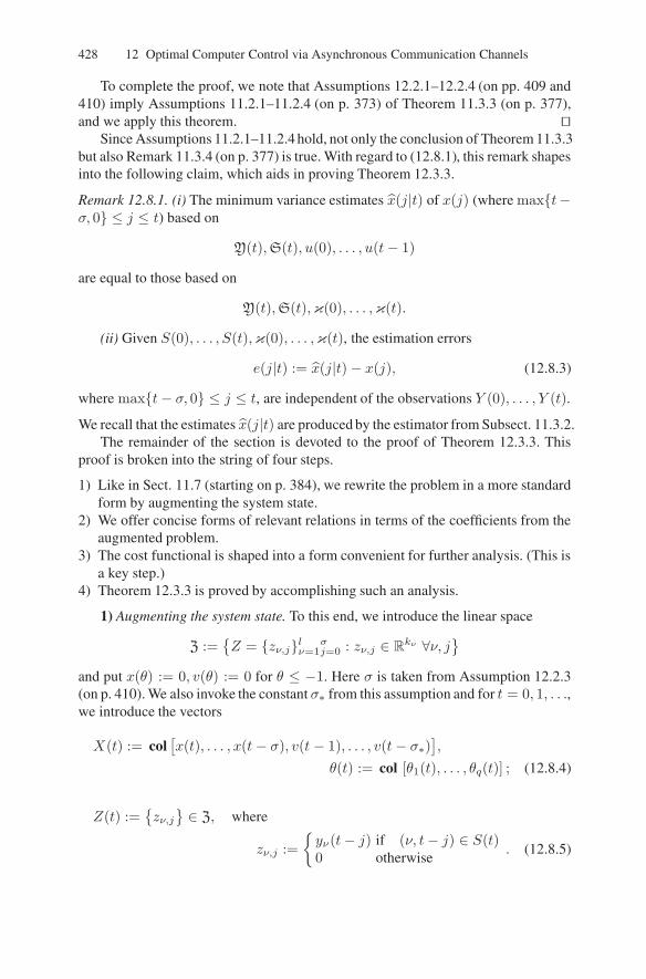
428 12 Optimal Computer Control via Asynchronous Communication Channels
To complete the proof, we note that Assumptions 12.2.1–12.2.4 (on pp. 409 and410) imply Assumptions 11.2.1–11.2.4 (on p. 373) of Theorem 11.3.3 (on p. 377),and we apply this theorem. ⊓⊔
but also Remark 11.3.4 (on p. 377) is true. With regard to (12.8.1), this remark shapesinto the following claim, which aids in proving Theorem 12.3.3.
Remark 12.8.1. (i) The minimum variance estimates x(j|t) of x(j) (where maxt−σ, 0 ≤ j ≤ t) based on
Y(t),S(t), u(0), . . . , u(t− 1)
are equal to those based on
Y(t),S(t),κ(0), . . . ,κ(t).
(ii) Given S(0), . . . , S(t),κ(0), . . . ,κ(t), the estimation errors
e(j|t) := x(j|t)− x(j), (12.8.3)
where maxt− σ, 0 ≤ j ≤ t, are independent of the observations Y (0), . . . , Y (t).
We recall that the estimates x(j|t) are produced by the estimator from Subsect. 11.3.2.The remainder of the section is devoted to the proof of Theorem 12.3.3. This
proof is broken into the string of four steps.
1) Like in Sect. 11.7 (starting on p. 384), we rewrite the problem in a more standardform by augmenting the system state.
2) We offer concise forms of relevant relations in terms of the coefficients from theaugmented problem.
3) The cost functional is shaped into a form convenient for further analysis. (This isa key step.)
4) Theorem 12.3.3 is proved by accomplishing such an analysis.
1) Augmenting the system state. To this end, we introduce the linear space
Z :=Z = zν,jlν=1
σj=0 : zν,j ∈ R
kν ∀ν, j
and put x(θ) := 0, v(θ) := 0 for θ ≤ −1. Here σ is taken from Assumption 12.2.3(on p. 410). We also invoke the constant σ∗ from this assumption and for t = 0, 1, . . .,we introduce the vectors
X(t) := col[x(t), . . . , x(t− σ), v(t − 1), . . . , v(t− σ∗)
],
θ(t) := col [θ1(t), . . . , θq(t)] ; (12.8.4)
Z(t) :=zν,j∈ Z, where
zν,j :=
yν(t− j) if (ν, t− j) ∈ S(t)0 otherwise
. (12.8.5)
Since Assumptions 11.2.1–11.2.4 hold, not only the conclusion of Theorem 11.3.3

12.8 Proofs of Theorem 12.3.3 and Remark 12.3.1 429
In terms of these vectors, the problem under consideration takes the form:
minimize I := E
T−1∑
t=0
G [t,X(t+ 1), v(t)] , where
G [t,X, v] := X TQ(t+ 1)X + v TΓ(t)v, (12.8.6)
subject to the constraints
X(t+ 1) = Aθ(t)(t)X(t) + Bθ(t)(t)v(t) + E ξ(t) t = 0, . . . , T − 1; (12.8.7)
X(0) = a := col (a, 0, . . . , 0); (12.8.8)
Z(t) = C[t, S(t)
]X(t) + Ξ
[t, S(t)
]t = 0, . . . , T ; (12.8.9)
v(t) = V [t, Z(0), . . . , Z(t), S(0), S(1), . . . , S(t),κ(0), . . . ,κ(t)] . (12.8.10)
Here for any t = 0, . . . , T and θ = col (θ1, . . . , θq), θi = 0, . . . , σ∗,
Q(t) :=
Q(t) 0 · · · 00 0 · · · 00 0 · · · 0· · · · · ·0 0 · · · 0
,
Bθ(t) := col[B0θ(t), 0, . . . , 0
∣∣Im, 0, . . . , 0],
E := col[In, 0, . . . , 0
];
(12.8.11)
Aθ(t) :=
A(t) 0 · · · 0 0In 0 · · · 0 00 In · · · 0 0
. . . . . . . . . . . . . . .0 0 · · · In 0
B1θ(t) · · · B
σ∗−1θ (t) B
σ∗θ (t)
0 · · · 0 00 · · · 0 0
. . . . . . . . . . . . . . . . . . . . . . . . .0 · · · 0 0
00 · · · 0 0Im · · · 0 00 · · · 0 0
. . . . . . . . . . . . . . . . . . . . . . . . .0 · · · Im 0
. (12.8.12)
The lines within matrices separate their “x”- and “v”- parts, and the matrices Bjθ(t)
are defined by (12.3.6) and (12.3.8) (on p. 413). Furthermore for any
t ≤ T, S ⊂ (ν, j) : ν ∈ [1 : l], j ∈ [0 : σ], X = col (x0, x1, . . . , xσ, v1, . . . , vσ∗),
the following relations hold:
C[t, S]X := zν,jlν=1σj=0 ∈ Z, where
zν,j :=
Cν(t− j)xj if (ν, t− j) ∈ S0 otherwise
; (12.8.13)

430 12 Optimal Computer Control via Asynchronous Communication Channels
Ξ[t, S] := ζν,jlν=1σj=0 ∈ Z, where
ζν,j :=
χν(t− j) if (ν, t− j) ∈ S0 otherwise
. (12.8.14)
When dealing with the augmented system, it is natural to employ the minimumvariance estimate
X(t|t) = E[X(t)
∣∣Z(0), . . . , Z(t), S(0), . . . , S(t),κ(0), . . . ,κ(t)]. (12.8.15)
Thanks to (i) of Remark 12.8.1, (12.8.4), (12.8.5), and (12.8.10),
X(t|t)= col [x(t|t), x(t− 1|t), . . . , x(t− σ|t), v(t − 1), . . . , v(t− σ∗)] . (12.8.16)
So the estimation error can be expressed in terms of (12.8.3):
E(t) := X(t|t)−X(t)
= col [e(t|t), e(t− 1|t), . . . , e(t− σ|t), 0, . . . , 0] . (12.8.17)
2) Concise form of relations (12.3.10)–(12.3.17) (on pp. 413 and 414). This formis in terms of the coefficients from (12.8.6) and (12.8.7), along with the followingmatrices:
H(t,κ) :=
Hxx(t,κ) 0 · · · 00 0 · · · 0
. . . . . . . . . . . . . . . .0 0 · · · 0
Hx1(t,κ) · · · Hxσ∗(t,κ)0 . . . 0
. . . . . . . . . . . . . . . . . . . . . . .0 · · · 0
H1x(t,κ) 0 . . . 0H2x(t,κ) 0 . . . 0. . . . . . . . . . . . . . . . .Hσ∗x(t,κ) 0 . . . 0
H11(t,κ) . . . H1σ∗(t,κ)H21(t,κ) . . . H2σ∗(t,κ). . . . . . . . . . . . . . . . . . . . . . . . .Hσ∗1(t,κ) . . . Hσ∗σ∗(t,κ)
; (12.8.18)
L(t,κ) :=[L(t,κ), 0, . . . , 0
∣∣L1(t,κ), . . . ,Lσ∗(t,κ)]. (12.8.19)
Here the partitions correspond to (12.8.12). We recall that κ is the tuple (12.3.2)(on p. 412) and the operations Pt,κ and ⊕ are defined by (12.3.5) and (12.3.7) (onp. 413), respectively.
Lemma 12.8.2. Suppose that t = 0, . . . , T − 1 and κ = [κ0, . . . ,κσ] ∈ Υσ+1
are given. Let the dot · stand for the variable κ ∈ Υ. We also invoke the notationθ(κ,κ) defined by (12.3.9) (on p. 413) and Notation 12.2.10 (on p. 411). Then thefollowing statements hold:
(i) The matrix F (t,κ) introduced in (12.3.4) (on p. 412) is positive-definite and
F (t,κ) = Pt,κ
Γ(t) + Bθ(·,κ)(t)
T[H(t+ 1, ·⊕ κ)
+ Q(t+ 1)]Bθ(·,κ)(t)
; (12.8.20)

12.8 Proofs of Theorem 12.3.3 and Remark 12.3.1 431
F (t,κ)L(t,κ) = Pt,κ
Bθ(·,κ)(t)
T[H(t+ 1, ·⊕ κ)
+ Q(t+ 1)]Aθ(·,κ)(t)
; (12.8.21)
H(t,κ) = L(t,κ) TΓ(t)L(t,κ)+
Pt,κ
[Aθ(·,κ)(t)−Bθ(·,κ)(t)L(t,κ)
] T[H(t+ 1, ·⊕ κ)
+ Q(t+ 1)] [
Aθ(·,κ)(t)−Bθ(·,κ)(t)L(t,κ)]. (12.8.22)
We recall that the matrices Bθ(t),Q(t+ 1), and Aθ(t) are defined by (12.8.11)and (12.8.12).
(ii) For any X = col (x0, . . . , xσ, v1, . . . , vσ∗) and v ∈ Rm, we put
X+(·) := Aθ(·,κ)(t)X + Bθ(·,κ)(t)v.
Then
Pt,κ
X+(·) T [H(t+ 1, ·⊕ κ) + Q(t+ 1)]X+(·)
−X TH(t,κ)X
+ v TΓ(t)v = [v + L(t,κ)X ]TF (t,κ) [v + L(t,κ)X ] . (12.8.23)
Proof. Statement (i). Note first that (12.3.5) (on p. 412), (12.8.22), and the bound-ary condition H(T,κ) = 0 imply recursively that H(t,κ) ≥ 0. Then (12.3.5) and(12.8.20) yield F (t,κ) > 0. Rewriting relations (12.8.20)–(12.8.22) in terms of theentries from (12.8.11), (12.8.12), (12.8.18), and (12.8.19) demonstrates that theserelations are merely another form of (12.3.10)–(12.3.17) (on pp. 413 and 414).
Statement (ii) By (12.8.22),
Pt,κ
Aθ(·,κ)(t)
T [H(t+ 1, ·⊕ κ) + Q(t+ 1)] Aθ(·,κ)(t)
− H(t,κ)
= L(t,κ) TPt,κ
Bθ(·,κ)(t)
T [H(t+ 1, ·⊕ κ) + Q(t+ 1)] Aθ(·,κ)(t)
−L(t,κ) TPt,κ
Γ(t)+Bθ(·,κ)(t)
T [H(t+ 1, ·⊕ κ) + Q(t+ 1)] Bθ(·,κ)(t)
L(t,κ)
+ Pt,κ
Aθ(·,κ)(t)
T [H(t+ 1, ·⊕ κ) + Q(t+ 1)]Bθ(·,κ)(t)
L(t,κ)
(12.8.20), (12.8.21)========= L(t,κ)F (t,κ)L(t,κ) T.

432 12 Optimal Computer Control via Asynchronous Communication Channels
In view of this, relationship (12.8.23) is immediate from (12.8.20) and (12.8.21). ⊓⊔
3) Transformation of the cost functional. This transformation plays a key role inproving Theorem 12.3.3.
Lemma 12.8.3. Suppose that a control strategy (12.8.10) is chosen. Consider theestimates (12.8.15) and put
κ(t) := [κ(t), . . . ,κ(t− σ)],
where σ is the constant from Assumption 12.2.8 (on p. 411). We recall that κ(s) isdefined for s < 0 by Remark 12.2.6 and (12.2.10) (on p. 410). For any t = 0, . . . , T ,the following representation of the cost functional from (12.8.6) holds:
I = E
t−1∑
s=0
G[s,X(s+ 1), v(s)] + EX(t) TH[t,κ(t)]X(t)
+ E
T−1∑
s=t
[v(s) + L[s,κ(s)]X(s|s)
] T
F [s,κ(s)]
×[v(s) + L[s,κ(s)]X(s|s)
]+ ∆(t), (12.8.24)
where
∆(t) := trT−1∑
s=t
E(L[s,κ(s)] TF [s,κ(s)]L[s,κ(s)]P 00(s)
)
+(Q(s+ 1) + EHxx[s+ 1,κ(s+ 1)]
)Rξξ(s)
. (12.8.25)
Here P 00(s) is the matrix generated by the estimator from Subsect. 11.3.2 (start-ing on p. 375 ), and Rξξ(t) is the disturbance correlation matrix from (12.2.9) (onp. 409).
Proof. The proof will be by induction on t = T, T − 1, . . . , 0. For t = T , (12.8.24)is immediate from (12.8.6), (12.8.18), and the boundary condition H(T,κ) = 0 ⇔H(T,κ) = 0. Suppose that (12.8.24) holds for t := t+ 1 ≤ T ; i.e.,
I = E
t−1∑
s=0
G[s,X(s+ 1), v(s)] + Ev(t) TΓ(t)v(t) + ∆(t+ 1)
+ EX(t+ 1) T H[t+ 1,κ(t+ 1)] + Q(t+ 1)︸ ︷︷ ︸N(t+1)
X(t+ 1)
+ E
T−1∑
s=t+1
[v(s) + L[s,κ(s)]X(s|s)
] T
F [s,κ(s)][v(s) + L[s,κ(s)]X(s|s)
].

12.8 Proofs of Theorem 12.3.3 and Remark 12.3.1 433
By (12.8.7),X(t+ 1) = X+(t) + Eξ(t),
where the vectorX+(t) := Aθ(t)(t)X(t) + Bθ(t)(t)v(t)
and the quantity κ(t+ 1) are independent of ξ(t) due to Assumptions 12.2.1, 12.2.2(on pp. 409 and 410), (12.8.7), (12.8.9), and (12.8.10). Since Eξ(t) = 0, this yields
EX(t+ 1) TN(t+ 1)X(t+ 1) = EX+(t) TN(t+ 1)X+(t)
+ Eξ(t) TE TN(t+ 1)Eξ(t). (12.8.26)
Owing to (12.2.9) (on p. 409), (12.8.11), and (12.8.18), the second summand on theright amounts to
Eξ(t) THxx[t+ 1,κ(t+ 1)] +Q(t+ 1)
ξ(t)
= tr[Q(t+ 1) + EHxx[t+ 1,κ(t+ 1)]
Rξξ(t)
].
To compute the first one, note that by (12.3.9) (on p. 413) and (12.8.2), θ(t) =θ[κ(t + 1),κ(t)]. Due to (12.8.7), (12.8.9), and (12.8.10), X(t) and v(t) are deter-ministic functions of
Π := [a, χν(0)lν=1, . . . , χν(t)lν=1, ξ(0), . . . , ξ(t− 1), S(0), . . . , S(t)]
and κ(0), . . . ,κ(t), where Π and κ(s) are independent thanks to Assump-tions 12.2.1 and 12.2.2 (on pp. 409 and 410). Hence putting K := [κ(α), . . . ,κ(t)],where α := maxt− σ, 0, we get
E[X+(t) TN(t+ 1)X+(t)
∣∣X(t) = X, v(t) = v,K]
=
E
[Aθ[κ(t+1),κ(t)]X + Bθ[κ(t+1),κ(t)]v
] T[H[t+ 1,κ(t+ 1)] + Q(t+ 1)
]
×[Aθ[κ(t+1),κ(t)]X + Bθ[κ(t+1),κ(t)]v
]∣∣∣∣∣K
(12.3.7)===
∑
κ∈Υ
P[κ(t+1) = κ
∣∣K][
Aθ[κ,κ(t)]X+Bθ[κ,κ(t)]v] T[
H[t+1,κ⊕κ(t)]+Q(t+1)]
×[Aθ[κ,κ(t)]X + Bθ[κ,κ(t)]v
].
Here P[κ(t + 1) = κ
∣∣K]
= P[κ(t + 1) = κ
∣∣κ(t)]
by Assumption 12.2.8 (onp. 411). So invoking (12.3.5) (on p. 412) shows that the conditional expectation underconsideration equals

434 12 Optimal Computer Control via Asynchronous Communication Channels
Pt,κ(t)
[Aθ[·,κ(t)]X + Bθ[·,κ(t)]v
] T[H[t+ 1, ·⊕ κ(t)] + Q(t+ 1)
]
×[Aθ[·,κ(t)]X + Bθ[·,κ(t)]v
]
(12.8.23)=== X
TH [t,κ(t)]X − v TΓ(t)v
+v + L [t,κ(t)]X
TF [t,κ(t)]
v + L [t,κ(t)]X
.
Thus in (12.8.26), the first summand on the right equals
EX(t) TH[t,κ(t)]X(t)−Ev(t)Γ(t)v(t) + µ(t), where
µ(t) := Ev(t) + L[t,κ(t)]X(t)
T
F [t,κ(t)]v(t) + L[t,κ(t)]X(t)
.
Now we employ the notation E(t) from (12.8.17) and denote
Λ := [S(0), . . . , S(t),κ(0), . . . ,κ(t)]. (12.8.27)
Then
µ(t) = Ev(t) + L[t,κ(t)]X(t|t)︸ ︷︷ ︸
w(t)
−L[t,κ(t)]E(t) T
F [t,κ(t)]
×w(t) − L[t,κ(t)]E(t)
= Ew(t) TF [t,κ(t)]w(t) + EE(t) TL[t,κ(t)] TF [t,κ(t)]L[t,κ(t)]E(t)
− 2EE[w(t) TF [t,κ(t)]L[t,κ(t)]E(t)
∣∣∣Λ]. (12.8.28)
Due to (12.8.10) and (12.8.15), w(t) is a deterministic function of Λ and Z(0), . . . ,Z(t). At the same time, E(t) is independent ofZ(0), . . . , Z(t) given Λ, and EE(t) =0 due to (ii) of Remark 12.8.1, (12.8.5), and (12.8.17). Hence the last summand onthe right in (12.8.28) is zero. The second one equals
δ := tr EL[t,κ(t)] TF [t,κ(t)]L[t,κ(t)]E
[E(t)E(t) T
∣∣Λ].
By Assumption 12.2.2 (on p. 410), the S and κ-parts of (12.8.27) are independent.At the same time, Remark 12.3.1 (on p. 411) and the last claim of Theorem 11.3.3 (onp. 377) guarantee that the estimation error (12.8.17) is not affected by the controls.Hence it is not influenced by κ(0), . . . ,κ(t). It follows that
E[E(t)E(t) T
∣∣Λ]
= E[E(t)E(t) T
∣∣S(0), . . . , S(t)].
By Remark 12.3.1, Theorem 11.3.3, and (12.8.17), the conditional expectation onthe right amounts to

12.9 Proof of Theorem 12.6.2 435
P 00(t) · · · P 0σ(t). . . . . . . . . . . . . . . . .P σ0(t) · · · P σσ(t)
00 0
.
In view of (12.8.19), this yields
δ = tr EL[t,κ(t)] TF [t,κ(t)]L[t,κ(t)]P 00(t)
.
Summarizing, we arrive at (12.8.24). ⊓⊔
4) Completion of the proof of Theorem 12.3.3 (on p. 414). By (i) of Lemma 12.8.2and (12.8.8) and (12.8.18), relation (12.8.24) with t := 0 implies that for any controlstrategy (12.8.10),
I ≥ ∆(0) + Ea THxx[0,κ(0)]a.
By (12.8.25), the obtained lower bound does not depend on the control. This boundis evidently attained at the strategy v(t) = −L[t,κ(t)]X(t|t), which equals (12.3.1)(on p. 411) thanks to (12.8.16) and (12.8.19). ⊓⊔
Concluding remarks. The representation (12.8.6)–(12.8.10) moves the problemunder consideration into the area of LQG control of systems whose coefficients aredetermined by a finite-state Markov chain.4 This area has received considerable at-tention (see, e.g., [1, 35, 36, 56, 79], we refer the reader to [36, 67, 78] for a survey).It however was mainly focused on continuous-time case, noise-free discrete-timesystems, or systems with incomplete observation of the Markov parameters. In thecorresponding literature, the authors failed to find a reference that directly provesTheorem 12.3.3. In view of this, we offered an independent proof, which is based onthe standard technique.
12.9 Proof of Theorem 12.6.2 on p. 424
The proof is based on the state augmenting technique considered in Sect. 11.7 (start-ing on p. 384). Like in that section, we introduce the linear space
Z :=Z = zν,jlν=1
σj=0 : zν,j ∈ R
kν ∀ν, j,
where l and σ are taken from (12.2.2) (on p. 407) and Assumption 12.4.1 (on p. 417),respectively, and put
x(θ) := 0, u(θ) := 0, A(θ) := I, B(θ) := 0 ∀θ ≤ −1.
Then formula (12.6.1) (on p. 421) makes sense for j = t + 1 − σ, . . . , t + 1 + σand t = 0, 1, . . .. For any τ ≥ 0, we consider the process x(t, τ) that is identical to
4Indeed, the tuples r(t) := [κ(t + 1), κ(t), . . . , κ(t − σ + 1)] form such a chain dueto Assumption 12.2.8 (on p. 411). At the same time, θ(t) = Θ[r(t)] by (12.8.2), whereΘ[κ0, κ1, . . . , κσ] := θ−(κ0) + θ+(κ1) and θ±(·) is defined by (12.2.11) (on p. 410).So in (12.8.7), the coefficients Aθ(t)(t) and Bθ(t)(t) are deterministic functions of t and r(t).

436 12 Optimal Computer Control via Asynchronous Communication Channels
x(t) until t = τ − σf + 1 and then proceeds in correspondence with the system’suncontrolled dynamics. We also denote
X(t) := col[x(t+σ, t), . . . , x(t−σ, t)
], Ω(t) := col
[ω(t+σ, t), . . . , ω(t−σ, t)
];
∆η(t) := col[δη(t+ σ + 1|t), . . . , δη(t− σ + 1|t)
]η = 1, 2;
W (t) :=wν,j
∈ Z, wν,j :=
yν(t− j) if (ν, t− j) ∈ S(t)0 otherwise
. (12.9.1)
It is easy to check that the evolution of this vectors is governed by the equations
X(t+ 1) = A(t)X(t) + B(t)u(t+ 1− σf ) + Eξ(t+ σ), X(0) = Ω0; (12.9.2)
Ω(t+1) = A(t)Ω(t)+D(t)[∆1(t)−∆2(t)
]+Eξ(t+σ), Ω(0) = Ω0; (12.9.3)
∆1(t+ 1) = A11∆ (t)∆1(t) + A12
∆ (t)∆2(t) + B1∆(t)u(t+ 1− σf ),
∆1(0) = 0; (12.9.4)
∆2(t+ 1) = A22∆ (t)∆2(t) + B2
∆(t)u(t+ 1− σf ), ∆2(0) = 0; (12.9.5)
W (t) = C[t, S(t)
]X(t) + Ξ
[t, S(t)
]t = 0, . . . , T. (12.9.6)
Here
A(t) :=
A(t+ σ) 0 · · · 0 0I 0 · · · 0 00 I · · · 0 0· · · · · · ·0 0 · · · I 0
, D(t) :=
the unit matrix ift+ 1 = f(t+ 1)t+ 1 6= f
and the zero matrixotherwise
, (12.9.7)
where f is defined by (12.5.5) (on p. 420) and the size of D(t) equals that of A(t).Furthermore,
Aηη∆ (t) :=
A(t+ 1) if
t ≥ σf + (η − 1)f − 1 and[t+ 1 6= f(t+ 1) or t+ 1 = f
]
0 if
t+ 1 < σf + (η − 1)f or
t+ 1 = νf for some ν = 2, 3, . . .
;
E := col (I, 0, . . . , 0), A12∆ (t) :=
A(t+ 1) if t+ 1 = f(t+ 1), t+ 1 6= f
0 otherwise;
B(t) := B〈σ〉(t), B1∆(t) := B〈σ+1〉(t), where
B〈s〉(t) := col[As,As−1, . . . ,A2−σf
, I, 0, . . . , 0]B(t+ 1− σf );
Aη :=
η∏
j=2−σf
A(t+ j); (12.9.8)

12.9 Proof of Theorem 12.6.2 437
B2∆(t) :=
B1
∆(t) if t+ 1 ≥ σ−(t+ 1) + f + σf
0 otherwise;
Ω0 := col [x0(σ), x0(σ − 1), . . . , x0(0), 0, . . . , 0] . (12.9.9)
Here x0(0), x0(1), . . . are determined recursively
x0(0) := a, x0(t+ 1) = A(t)x0(t) + ξ(t)
and for any
t ≤ T, S ⊂ (ν, j) : ν = 1, . . . , l, j = 0, . . . , σ, X = col (x−σ , x−σ+1, . . . , xσ),
the following relations hold:
C[t, S]X := wν,jlν=1σj=0 ∈ Z, where
wν,j :=
Cν(t− j)xj if (ν, t− j) ∈ S0 otherwise
; (12.9.10)
Ξ[t, S] := ζν,jlν=1σj=0 ∈ Z, where
ζν,j :=
χν(t− j) if (ν, t− j) ∈ S0 otherwise
. (12.9.11)
By (12.4.5) (on p. 417),
ui(tc) = Ui[tc,Y(τ),S(τ), θ(0), . . . , θ(tc)] for tc := t+ 1− σf ,
where Y(τ),S(τ) are defined in (12.2.8) (on p. 409), τ := tc − θi(tc) ≤ t, and
θ(s) := col [θ1(s), . . . , θq(s)] .
Hence in (12.9.2)–(12.9.5),
u(t+1−σf ) = U[t,W (0), . . . ,W (t),S(t), θ(0), . . . , θ(t+ 1− σf )
], (12.9.12)
where U(·) is a deterministic function. By Assumption 12.2.2 (on p. 410), the ran-dom sets S(t) from (12.4.2) (on p. 415) and the tuples of the delays θ(t) areindependent of a, ξ(t), and χν(t). Then (12.2.3) (on p. 408) and (12.9.9) implythat the vectors Ω0, ξ(t+ σ), and Ξ[t, S(t)] conditioned over
S(0), . . . , S(T − 1) and θ(0), . . . , θ(T − 1)
are (singular) Gaussian and independent. This and (12.9.2), (12.9.6), and (12.9.12)imply that the estimate
X(t) := E[X(t)
∣∣∣W (0), . . . ,W (t), S(0), . . . , S(T − 1), θ(0), . . . , θ(T − 1)]

438 12 Optimal Computer Control via Asynchronous Communication Channels
is generated by the ordinary Kalman filter (see Subsect. C.2 in Appendix C). Byinvoking the corresponding formulas (C.8)–(C.13) (on pp. 510 and 511) , it is easy tosee that only the sets S(0), . . . , S(t) (and the delays θ(0), . . . , θ(t−σf ) if t ≥ σf ) areused to compute X(t). So in view of (12.4.2) (on p. 415), (12.9.1), and the definitionof Υ(t) from (12.6.15) (on p. 424),
Z(t) = E[Z(t)
∣∣∣Y(t),S(t),Υ(t)],
where Y(t) and S(t) are defined in (12.2.8) (on p. 409). Furthermore (12.9.2) and(12.9.3) yield
Ω(t+ 1)−X(t+ 1) = A(t) [Ω(t)−X(t)]
+ D(t)[∆1(t)−∆2(t)
]−B(t)u(t + 1− σf )︸ ︷︷ ︸
Zt+1
, Ω(0)−X(0) = 0,
where Zt is a deterministic function of Y(t),S(t) and Υ(t). Hence
Ω(t+1)−X(t+1) = A(t)[Ω(t)− X(t)
]+Zt+1, Ω(0)−X(0) = 0, (12.9.13)
and X(t) − X(t) = Ω(t) − Ω(t), where Ω(t) := E[Ω(t)
∣∣∣Y(t),S(t),Υ(t)]. By
the Kalman filter formulas (C.8)–(C.13), X(t) obeys the first equation from (12.9.2)where the noise Eξ(t+σ) is replaced by a correction term δ generated by the Kalmanfilter. Thanks to (12.9.13), Ω(t) obeys the first equation from (12.9.3) where the noiseis replaced by the same term δ.
The statement of Theorem 12.6.2 (on p. 424) results from putting the expres-sions (12.9.1)–(12.9.11) into the equations (C.8)–(C.13) (on pp. 510 and 511) of theconventional Kalman filter, along with elementary transformations of the resultantformulas and taking into account (iv) of Theorem C.2 (on p. 511) in Appendix C.
12.10 Proofs of Theorem 12.7.1 and Proposition 12.7.2
From now on, Assumptions 12.2.1, 12.2.2, and 12.4.1–12.4.4 (on pp. 409, 410, 417,and 418) are supposed to hold. This section is organized as follows. Its first andsecond subsections contain auxiliary lemmas and the proof of Theorem 12.7.1 (onp. 426) in the case of a single subsystem, respectively. The proof of this theoremin the general case is offered in the third subsection, where Proposition 12.7.2 (onp. 427) is also proved.
12.10.1 Preliminaries
We recall that θi(t) is the time elapsed since the departure of the control messagecurrently employed by the ith subsystem. If no message has arrived until t, thenθi(t) := t+ 1. Furthermore, θ(t) := col
[θ1(t), . . . , θq(t)
].

12.10 Proofs of Theorem 12.7.1 and Proposition 12.7.2 439
Lemma 12.10.1. For any i = 1, . . . , q and t = 0, . . . , T , the inequality θi(t) ≤σi + µi − 1 holds. Here σi and µi are the constants from Assumptions 12.4.1 and12.4.2 (on pp. 417 and 417), respectively.
Proof. Put s := t−θi(t). Assumption 12.4.2 ensures that among the messages m(s)dispatched via the ith control channel at times s = s + 1, . . . , s + µi, there is atleast one m′ = m(s′) that reaches the ith subsystem. Let t′ denote its arrival time.If s = −1, the subsystem has received no message until t and thus t′ > t. Supposethat s ≥ 0 and denote by m the message employed by the subsystem at the time t.It was departed at s < s′, and so it is less updated than m′. Employed is the mostupdated message arrived until t. Thus t′ > t; i.e., this inequality holds in any case.By Assumption 12.4.1 (on p. 417), t′ − s′ ≤ σi. Thus
s+ θi(t) = t < t′ ≤ s′ + σi ≤ s+ µi + σi ⇒ θi(t) < µi + σi,
which completes the proof. ⊓⊔
Lemma 12.10.2. Suppose that a control strategy (12.4.5) (on p. 417) is chosen. Con-sider the corresponding process in the system (12.2.1), (12.2.2) (on p. 407), theoutput (12.5.8) (on p. 420) of the state estimator described in Sect. 12.6, and theminimum variance estimates
xi(t) := E[xi(t)
∣∣Y(τ),S(τ), θ(0), . . . , θ(t)]; (12.10.1)
x0|i(t) := E[x0(t)
∣∣Y(τ),S(τ), θ(0), . . . , θ(t)], (12.10.2)
where τ := t− θi(t). Then for any i = 1, . . . , q, t = 0, . . . , T , we have
x0|i(t) = ω0[t|τ ], xi(t) = ωi[t|τ ] +
x(0)i (t) if t < f
x(2)i (t) if f ≤ τ < f(t)
x(1)i (t) otherwise
. (12.10.3)
Here col [ω0(j|t), . . . , ωq(j|t)] is the partition of ω(j|t) corresponding to (12.4.1)
(on p. 415) and f(t), x(η)i (t) are defined by (12.5.5) and (12.5.6) (on p. 420), respec-
tively.
Proof. Pick i = 1, . . . , q and put x0(t) := x0|i(t). Assumption 12.4.3 (on p. 418)and (12.5.2) (on p. 419) yield
xi(t) = ωi(t, τ) + λi(t, τ), where λi(t, τ) :=
t−1∑
r=σ−(τ)
t−1∏
ν=r+1
Ai(ν)Bi(r)ui(r)
for i ≥ 1, λ0(t, τ) := 0, and τ := t − θi(t). By (12.4.5) (on p. 417), λi(t, τ) is adeterministic function of Y(τ),S(τ), and θ(0), . . . , θ(t). This and (12.10.1) give
xi(t) = Eωi [t, τ ]
∣∣∣Y(τ),S(τ), θ(0), . . . , θ(t)
+ λi(t, τ).

440 12 Optimal Computer Control via Asynchronous Communication Channels
Due to (12.2.1), (12.2.3), (12.4.5), and (12.7.5) (on pp. 407, 408, 417, and 425),
ωi(t, τ) = Ωi [t, τ,Ξ,Y(τ),S(τ),Υ(τ)] ,
where Ξ :=[a, ξ(s)t−1
s=0
], the quantity Υ(τ) is defined in (12.6.15) (on p. 424),
and Ωi(·) is a deterministic function. Here the quantities θ(s) are independent ofΞ and H(s′) := [Y(s′),S(s′)] by Assumption 12.2.2 (on p. 410). So the followingrelation holds for the conditional distributions:
pdΞ|H[τ ], θ(0), . . . , θ(t)
= p dΞ|H(s)
∣∣s=t−θi(t)
= p dΞ|H(s),Υ(s)∣∣s=t−θi(t)
.
Therefore
Eωi [t, τ ]
∣∣∣H(τ), θ(0), . . . , θ(t)
= E
Ωi [t, τ,Ξ,H(τ),Υ(τ)]∣∣∣H(τ), θ(0), . . . , θ(t)
=
∫Ωi [t, τ,Ξ,H(τ),Υ(τ)] p[dΞ|H(τ), θ(0), . . . , θ(t)]
=
∫Ωi [t, s,Ξ,H(s),Υ(s)] p[dΞ|H(s),Υ(s)]
∣∣∣s=t−θi(t)
= Eωi [t, s]
∣∣∣Y(s),S(s),Υ(s) ∣∣∣
s=t−θi(t)
(12.6.14)==== ωi[t|t− θi(t)].
Then (12.10.3) is immediate from (12.5.5), (12.5.6), (12.7.5) (on pp. 420 and 425),and Lemma 12.10.1. ⊓⊔
12.10.2 Proof of Theorem 12.7.1 on p. 426: Single Subsystem
In this case, the subsystem’s serial number i can take only one value i = 1. Howeverin the formulas to follow, we employ the general notation i instead of using merely1. These formulas can actually be considered for any i in the general case of manysubsystems and will be utilized in the next subsection, where this case is discussed.
We are going to show first that the problem can be reduced to the standard LQGoptimal control problem. To this end, we denote σ := σi + µi + σ − 1, where σ, σi,and µi are taken from Assumptions 12.4.1 and 12.4.2 (on pp. 417 and 417), considerthe linear space
Z :=Z = zν,jlν=1
eσj=0 : zν,j ∈ R
kν ∀ν, j,
where l is taken from (12.2.2) (on p. 407) and kν is the dimension of the sensoroutput yν , and put
x(−σ) := x(−σ + 1) := · · · := x(−1) := 0, si(−1) := 0;

12.10 Proofs of Theorem 12.7.1 and Proposition 12.7.2 441
X(t) := col[x(t), x(t − 1), . . . , x(t− σ)
], W (t) :=
wν,j
∈ Z;
wν,j :=
yν(t− j) if (ν, t− j) ∈ S[τi(t)] and τi(t) > τi(t− 1)0 otherwise
,
(12.10.4)
where τi(t) := t− θi(t). In terms of these vectors, the primal problem shapes into
minimize E
T−1∑
t=0
[X(t+ 1) TQ(t+ 1)X(t+ 1) + ui(t)TΓi(t)ui(t)] subject to
(12.10.5)X(t+ 1) = A(t)X(t) + B(t)ui(t) + E ξ(t) t = 0, . . . , T − 1; (12.10.6)
X(0) = a := col (a, 0, . . . , 0); (12.10.7)
W (t) = Ct, S[τi(t)], θi(t), θi(t− 1)
X(t)
+ Ξt, S[τi(t)], θi(t), θi(t− 1)
; (12.10.8)
ui(t) =
Ui
W (0), . . . , W (t), S(0), S(1), . . . , S[t− θi(t)], θ(0), . . . , θ(t)
. (12.10.9)
Here τi(t) := t− θi(t) and E := col (I, 0, . . . , 0),
A(t) :=
A(t) 0 . . . 0 0I 0 . . . 0 00 I . . . 0 0· · · · · · ·0 0 . . . I 0
, Q(t) :=
Q(t) 0 · · · 00 0 · · · 00 0 · · · 0· · · · · ·0 0 · · · 0
, (12.10.10)
where Q(t) := Q(t) and Q(t) is taken from (12.2.6) (on p. 408). Furthermore,
B(t) := col[B(t), 0, . . . , 0
],
where the matrix B(t) := col [0, B1(t)] describes the influence of the control u1 onthe process x = col [x0, x1] and B1(t) is taken from (12.4.7) (on p. 418). For anyt ≤ T ,
S ⊂ (ν, j) : ν = 1, . . . , l, j = 0, . . . , σ, θ′ ≥ θ′′,and X = col (x0, x1, . . . , xeσ) ∈ R(eσ+1)n, the following relations hold:
C[t, S, θ′, θ′′]Z := C[S]X
Ξ[t, S, θ′, θ′′] := Ξ[t, S]
if t− θ′ > t− 1− θ′′,
otherwise,

442 12 Optimal Computer Control via Asynchronous Communication Channels
C[t, S, θ′, θ′′]Z := 0
Ξ[t, S, θ′, θ′′] := 0,
where C[S]X and Ξ[t, S] are defined by (12.9.10) and (12.9.11) (on p. 437) withσ := σ. The random sets S(j) and delays θi(j) are independent of a, ξ(j),χν(j) by Assumption 12.2.2 (on p. 410). So by (12.2.3) and (12.2.5) (on p. 408),the vectors a, ξ(t), and Ξt, S[τi(t)], θi(t), θi(t − 1) conditioned over S(0), . . .,S(T−1), θ(0), . . . , θ(T−1) are Gaussian and independent. This yields that the prob-lem resulting from (12.10.5)–(12.10.9) by expansion the class of admissible controls(12.10.9) as follows:
ui(t) = Ui
W (0), . . . , W (t), S(0), S(1), . . . , S(T − 1), θ(0), . . . , θ(T − 1)
in fact reduces to a particular case of the standard LQG optimal control problem (seeAppendix C starting on p. 509). The solution of the latter problem is given by thelinear feedbackui(t) = −L(t)X(t) that is optimal for the problem of minimizing thefunctional (12.10.5) subject to the constraints (12.10.6) in the case where ξ(t) ≡ 0and the entire state X is measured. This feedback is fed by the minimum varianceestimate X(t|t) of X(t) based on the observations W (0), . . . , W (t). This estimateis generated recursively by the Kalman filter (see Appendix C) so that only the setsS[0], . . . , S[t−θi(t)] and the tuples θ(0), . . . , θ(t) from (12.10.8) are in fact requiredto compute X(t|t). This in particular means that
X(t|t) = E(X [t]
∣∣∣W [j]
tj=0
,S[j]
t−θi(t)
j=0,θ[j]tj=0
). (12.10.11)
Calculating the gain matrix L(t) employs the coefficients of the functional (12.10.5)and the equation (12.10.6) for the time instants t, t+1, . . . , T . Since these coefficientsdo not depend on S(j), θ(j) and are known a priori, the control appears to be ofthe form (12.10.9). So it furnishes the optimum over the strategies given by (12.10.9).
By invoking the formulas for the solution of the standard linear-qudratic controlproblem (i.e., formulas (C.18)–(C.21) on p. 512), it is easy to check that the abovefeedback ui(t) = −L(t)X(t) has the form ui(t) = −L∗(t)x(t), where X(t) is thetuple from (12.10.4) and ui(t) = −L∗(t)x(t) is the optimal feedback for the problemof minimizing the functional (12.2.6) (on p. 408) subject to the constraints (12.2.1)(on p. 407) in the case where ξ(t) ≡ 0 in (12.2.1) and the entire state x = col [x0, x1]is measured. Likewise, it is straightforward to verify that the last feedback looks asfollows:
ui(t) = −Li(t)xi(t)− Li(t)x0(t),
where Li(t), Li(t) are defined by (12.7.1)–(12.7.4) (on p. 424). Summarizing we seethat the solution for the initial problem is given by
ui(t) = −Li(t)ˆxi(t)− Li(t)ˆx0(t),
where

12.10 Proofs of Theorem 12.7.1 and Proposition 12.7.2 443
ˆxj := Exj(t)|W [0], . . . , W [t], S[0], . . . , S[t− θi(t)], θ(0), . . . , θ(t).
Invoking (12.2.3) (on p. 408) and (12.10.4) demonstrates that
ˆxj := Exj(t)|Y[τ ],S[τ ], θ(0), . . . , θ(t),
where τ = t− θi(t), and by (12.10.1) and (12.10.2), the optimal feedback takes theform
ui(t) = −Li(t)xi(t)− Li(t)x0|i(t).
Employing (12.10.3) shapes this formula into
ui(t) = −Li[τ + θi(t)]ωi[τ + θi(t)|τ ] + Li[τ + θi(t)]ω0[τ + θi(t)|τ ]
− Li(t)×
x(0)i (t) if t < f
x(2)i (t) if f ≤ t− θi(t) < f(t)
x(1)i (t) otherwise
. (12.10.12)
Now consider the control algorithm described in Sect. 12.7 (starting on p. 424). Bythe definition of θi(t), the control package currently used by the local controller wasdeparted at the time τ . So by (12.7.7) (on p. 425), the summand in the curly brackets· · · from (12.10.12) equals the member v(i)
θi(t)of this package. Here θi(t) = τi+si,
where τi and si are the numbers generated by the ith local controller. It follows that(12.10.12) takes the form (12.7.8) (on p. 426). ⊓⊔
12.10.3 Proofs of Theorem 12.7.1 and Proposition 12.7.2: Many Subsystems
We start with a lemma that was in fact proved in the case of a single subsystem inthe preceding subsection.
Lemma 12.10.3. Let i = 1, . . . , q be given, and let any subsystem except for theith one be controlled in accordance with some given strategy of the form (12.4.5)(on p. 417). Consider the problem (12.7.9) (on p. 426) of optimal control of the ithsubsystem, where the control strategy is sought in the class (12.4.5) with i fixed. Thesolution for this problem is given by the feedback
ui(t) = −Li(t)xi(t)− Li(t)x0|i(t). (12.10.13)
Here xi(t), x0|i(t) are the estimates (12.10.1), (12.10.2) and Li(t), Li(t) are definedby (12.7.1)–(12.7.4) (on p. 425).
Proof. For j = 1, . . . , q, consider the matrix
Bj(t) := col [0, . . . , 0, Bj(t), 0, . . . , 0]
that describes the influence of the jth control uj on the process x = col [x0, . . . , xq].Here the matrix Bj(t) is taken from (12.4.7) (on p. 418) and occupies the (j + 1)thposition. Introduce also the process x∗(t) generated by the equations

444 12 Optimal Computer Control via Asynchronous Communication Channels
x∗(t+ 1) = A(t)x∗(t) +∑
j 6=iBj(t)uj(t), x∗(0) = 0. (12.10.14)
In terms of the difference x(t) := x(t) − x∗(t), relations (12.2.1) and (12.2.2) (onp. 407) take the form:
x(t+1) = A(t)x(t)+Bi(t)ui(t)+ξ(t) t = 0, . . . , T−1, x(0) = a; (12.10.15)
yν(t) := yν(t)− Cν(t)x∗(t) = Cν(t)x(t) + χν(t), (12.10.16)
where ν = 1, . . . , l and t = 0, . . . , T . Put
Y (t) :=yν [θ]
(ν,θ)∈S(t)
, Y(t) := [Y (0), . . . , Y (t)].
We are going to show first that
Y(t) = Y [Y(t),F(t)] , Y(t) = Y
[Y(t),F(t)
], (12.10.17)
where F(t) := [S(t), θ(0), . . . , θ(t−1), t] and Y(t) is defined in (12.2.8) (on p. 409).(We recall that capital script letters denote deterministic functions.) For t = 0,(12.10.17) is evident since x∗(0) = 0 by (12.10.14). Let (12.10.17) be true for somet. If S(t+ 1) = ∅, then Y (t+ 1) = Y (t+ 1) = 0 ∈ R and so (12.10.17) does holdfor t := t+1. Suppose that S(t+1) 6= ∅. Due to (12.4.5) (on p. 417) and (12.10.14),
x∗(s) = X∗[Y(s− 1),S(s− 1), θ(0), . . . , θ(s− 1), s].
Hence for s ≤ t+ 1,
x∗(s) = X[Y(t),S(t), θ(0), . . . , θ(t), s
] (12.10.17)==== X
[Y(t),S(t), θ(0), . . . , θ(t), s
].
This and the definition of yν(t) from (12.10.16) clearly imply (12.10.17) for t :=t+ 1.
Relations (12.10.17) shape (12.4.5) (on p. 417) into
ui(t) = U
[t, Y(τ),S(τ), θ(0), . . . , θ(t)
]τ := t− θi(t). (12.10.18)
Let x = col (x0, . . . , xq) be the partition corresponding to (12.4.1) (on p. 415). For thesimilar partition x∗(t) = col [x∗,0(t), . . . , x∗,q(t)], Assumption 12.4.3 (on p. 418)and (12.10.14) imply that x∗,j(t) = 0 for j = 0, i. Hence
x0(t) = x0(t), xi(t) = xi(t) ∀t. (12.10.19)
So in view of (12.4.8) (on p. 418), the problem (12.7.9) (on p. 426) can be rewrittenin terms of the vector x(t):
minimize E
T−1∑
t=0
Gi[t, x(t+ 1), ui(t)]
subject to (12.10.15) and (12.10.16) (12.10.20)

12.10 Proofs of Theorem 12.7.1 and Proposition 12.7.2 445
over the control strategies (12.10.18). Here Gi(·) is taken from (12.4.8) (on p. 418).This problem can be reduced to a particular case of the standard LQG optimal
control problem just as it was done in Subsect. 12.10.2. Now one, however, shouldreplace (12.10.4) by
X(t) := col[x(t), x(t − 1), . . . , x(t− σ)
], W (t) :=
wν,j
∈ Z;
wν,j :=
yν(t− j) if
(ν, t− j) ∈ S[τi(t)] andτi(t) > τi(t− 1)
0 otherwise, (12.10.21)
where τi(t) := t− θi(t), put
x(−σ) := x(−σ + 1) := · · · := x(−1) := 0, θi(−1) := 0,
and define the matrices B(t) in (12.10.6) and Q(t) in (12.10.10) by the formulas
Q(t) :=
0 . . . Qi(t) . . . 0· · · · ·
Qi(t)T . . . Qi(t) . . . 0
· · · · ·0 . . . 0 . . . 0
, B(t) :=
Bi(t)0·0
.
Here the partition of the n × n matrix Q(t) corresponds to the partition of the statefrom (12.4.1), all three nonzero blocks of Q(t) belong to the ith row and column,and the enumeration of the rows and columns starts with 0.
By retracing the arguments from Subsect. 12.10.2, and invoking (12.10.19),wesee that the solution for the problem under consideration is given by the feedback
ui(t) = −Li(t)ˆxi(t)− Li(t)ˆx0(t),
where
ˆxj := Exj(t)|W [0], . . . , W [t], S[0], . . . , S[t− θi(t)], θ(0), . . . , θ(t).
Invoking (12.2.3) (on p. 408) and (12.10.21) demonstrates that
ˆxj := Exj(t)|Y[τ ],S[τ ], θ(0), . . . , θ(t),
where τ = t − θi(t). Relations (12.10.1), (12.10.2), and (12.10.17) complete theproof. ⊓⊔
Remark 12.10.4. For each i, the auxiliary problem considered in Lemma 12.10.3 wasintroduced under the assumption that the control strategies for all subsystems exceptfor the ith one are given. The minimum value of the cost functional in this problemdoes not depend on these strategies. This follows from, e.g., the fact that the problemcan be rewritten in the form (12.10.5)–(12.10.9), which is invariant with respect tothe above strategies.

446 12 Optimal Computer Control via Asynchronous Communication Channels
Proofs of Theorem 12.7.1 (on p. 426) and Proposition 12.7.2 (on p. 427). Lem-ma 12.10.3 and Remark 12.10.4 imply that the optimal way to control the ith sub-system is given by (12.10.13). This is true for not only the auxiliary problem (12.7.9)(on p. 426) associated with only this subsystem but also for the primal one concern-ing the entire set of subsystems. Denote τ := t − θi(t). Then relations (12.10.3)shape (12.10.13) into (12.10.12). Now consider the control algorithm described inSect. 12.7. By the definition of θi(t), the control package currently used by the ithlocal controller was departed at the time τ . So by (12.7.7) (on p. 425), the addendin the curly brackets from (12.10.12) equals the member v(i)
θi(t)of this package. Here
θi(t) = τi+si, where τi and si are the numbers generated by the ith local controller.It follows that (12.10.12) takes the form (12.7.8) (on p. 426). ⊓⊔

13
Linear-Quadratic Gaussian Optimal Control viaLimited Capacity Communication Channels
13.1 Introduction
In this chapter, we proceed with studying optimal control problems in the case wherecontrols are communicated via limited bandwidth channels. A situation of such akind has been addressed in Sect. 12.4. However the issue of limited bandwidth wastaken into account only implicitly to motivate distribution of control functions be-tween the central and local controllers. The objective of this chapter is to addressthis issue explicitly. In other words, now examined is the performance best in thecase where the bit-rate of the control channel is finite and given. Another distinctionis that now we examine the case where the actuators are basically capable only toexecute the currently received control signal, whereas actuators endowed with ratherpowerful computing modules were considered in Sect. 12.4. We also drop the systemdisintegration assumptions from Sect. 12.4 and deal with general linear plants.
Specifically, we study a finite-horizon linear-quadratic optimal control problemfor a discrete-time partially observed system with Gaussian disturbances. The con-troller produces a control signal based on the prior observations. Unlike the clas-sic linear-quadratic Gaussian (LQG) control problems (see Appendix C starting onp. 509), this signal is communicated to the actuators over a digital channel. This chan-nel is capable of transferring no more than a given number of bits of information perunit time. So on its way to the actuator, the control signal must be first encoded, thentransmitted, and finally decoded (see Fig. 13.1). The algorithms of encoding and de-coding are part of the control strategy, which should be designed to achieve the bestperformance. The focus is on memoryless (static) decoders. This corresponds to thecase where actuators are not equipped with computing and memory modules. Thecontroller has access to the sensor data with arbitrarily high accuracy, which may bedue to, e.g., the fact that it is colocated with the sensors. Unlike Chaps. 11 and 12,both observation and control channels provide no delays and dropouts.
We prove that the optimal strategy does exist (i.e., the minimum of the cost func-tional is attained) and demonstrate how this strategy can be designed. We also provethat the current optimal control codeword transmitted over the channel is determinedon the basis of the minimum variance estimate of the current state. In this sense, this
A.S. Matveev and A.V. Savkin, Estimation and Control over Communication Networks,
© Birkhäuser Boston, a part of Springer Science + Business Media, LLC 200
447 doi: 10.1007/978-0-8176-4607-3_13,
9
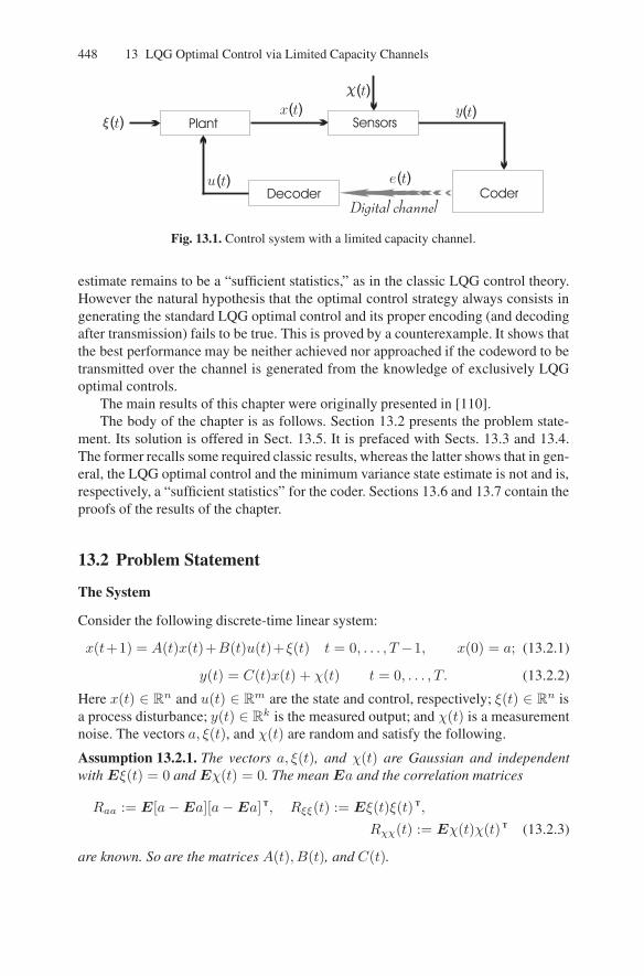
448 13 LQG Optimal Control via Limited Capacity Channels
Fig. 13.1. Control system with a limited capacity channel.
estimate remains to be a “sufficient statistics,” as in the classic LQG control theory.However the natural hypothesis that the optimal control strategy always consists ingenerating the standard LQG optimal control and its proper encoding (and decodingafter transmission) fails to be true. This is proved by a counterexample. It shows thatthe best performance may be neither achieved nor approached if the codeword to betransmitted over the channel is generated from the knowledge of exclusively LQGoptimal controls.
The main results of this chapter were originally presented in [110].The body of the chapter is as follows. Section 13.2 presents the problem state-
ment. Its solution is offered in Sect. 13.5. It is prefaced with Sects. 13.3 and 13.4.The former recalls some required classic results, whereas the latter shows that in gen-eral, the LQG optimal control and the minimum variance state estimate is not and is,respectively, a “sufficient statistics” for the coder. Sections 13.6 and 13.7 contain theproofs of the results of the chapter.
13.2 Problem Statement
The System
Consider the following discrete-time linear system:
x(t+1) = A(t)x(t)+B(t)u(t)+ξ(t) t = 0, . . . , T−1, x(0) = a; (13.2.1)
y(t) = C(t)x(t) + χ(t) t = 0, . . . , T. (13.2.2)
Here x(t) ∈ Rn and u(t) ∈ Rm are the state and control, respectively; ξ(t) ∈ Rn isa process disturbance; y(t) ∈ Rk is the measured output; and χ(t) is a measurementnoise. The vectors a, ξ(t), and χ(t) are random and satisfy the following.
Assumption 13.2.1. The vectors a, ξ(t), and χ(t) are Gaussian and independentwith Eξ(t) = 0 and Eχ(t) = 0. The mean Ea and the correlation matrices
Raa := E[a−Ea][a−Ea] T, Rξξ(t) := Eξ(t)ξ(t) T,
Rχχ(t) := Eχ(t)χ(t) T (13.2.3)
are known. So are the matrices A(t), B(t), and C(t).

13.3 Preliminaries 449
The Control Loop
The actuators are situated at a remote location, where the control signals are sent overa digital communication channel. It is able to transfer no more than a given numberb of bits per unit time. So the control must be in fact generated as an b-bit codeworde(t). This is done by the controller-coder on the basis of the prior observations:
e(t) = E[t, y(0), . . . , y(t)] ∈ E. (13.2.4)
(We recall that capital script letters denote deterministic functions.) Here E = eis the channel’s alphabet. Since the “physical” nature of the elements e now is of noimportance, we assume that E = [1 : N ], where N := 2b.1 The code-symbol e(t) istransmitted and then translated by a decoder into the “final” control signal u(t) thatacts upon the plant (see Fig. 13.1). We consider the case of a memoryless decoder:
u(t) = U[t, e(t)] ∈ Rm. (13.2.5)
Thus the control strategy consists of the coder (13.2.4) and the decoder (13.2.5).
LQG Optimal Control Problem with Communication Capacity Constraints
Introduce the functional
IT := E
T−1∑
t=0
[x(t+ 1) TQ(t+ 1)x(t+ 1) + u(t) TΓ(t)u(t)
]. (13.2.6)
Here Q(t + 1) ≥ 0 and Γ(t) > 0 are symmetric n × n and m × m matrices,respectively. In this chapter, we consider the following problem.
Let the bit-rate of the channel b be given. We wish to minimize the functional(13.2.6) over the class of control strategies described by (13.2.4) and (13.2.5).
In doing so, we consider only measurable functions E(·) in (13.2.4).
Remark 13.2.2. Putting (13.2.4) into (13.2.5) yields that
u(t) = V[t, y(0), . . . , y(t)].
For given t, the function V[t, ·] can take any values from Rm. However, their numbermust not exceed a given constant N . This makes the difference with the standardsetup of the stochastic optimal control problem (see, e.g., [11, 19, 85, 123,198]).
13.3 Preliminaries
The posed problem resembles the standard LQG optimal control problem2 in manyrespects. So it does not come as a surprise that the solutions of these two problemshave much in common. For the convenience of the reader, we repeat the relevantformulas concerning the standard LQG problem from Appendix C in this section.
1We do not suppose further that b is natural. So N is not necessarily a natural power of 2.2See Subsect. C.1 in Appendix C.

450 13 LQG Optimal Control via Limited Capacity Channels
Minimum Variance State Estimate
Let a control strategy (13.2.4), (13.2.5) be given. Then the state estimate
x(t|t) = E[x(t)
∣∣y(0), . . . , y(t)]
(13.3.1)
can be generated recursively by the Kalman filter:
x(t+ 1|t+ 1) := x(t+ 1|t) +K(t+ 1)[y(t+ 1)−C(t+ 1)x(t+ 1|t)
]; (13.3.2)
P (t+ 1) := A(t)P (t)A(t) T +Rξξ(t), where
x(t+ 1|t) := A(t)x(t|t) +B(t)u(t), P (t) := P (t)−K(t)C(t)P (t); (13.3.3)
K(t) := P (t)C(t) T+
Λ(t), Λ(t) := Λ := C(t)P (t)C(t) T +Rχχ(t), (13.3.4)
and+
Λ is the pseudoinverse of the matrix Λ (see Subsect. 11.3.1 starting on p. 374).The estimation process is initialized by putting
x(−1| − 1) := Ea, P (0) = Raa,
u(−1) := 0, B(−1) := 0, A(−1) := In. (13.3.5)
Solution for the Deterministic Linear-Quadratic Optimal Control Problem
We mean the problem of minimizing the functional (13.2.6) subject to the constraints(13.2.1) in the case where the process disturbances are removed (ξ(t) ≡ 0) and theentire state x is accessible for “on-line” measurements. The solution for this problemis given by the feedback u(t) = −L(t)x(t), where
L(t) = F (t)−1B(t) T [Q(t+ 1) +H(t+ 1)]A(t),
F (t) := Γ(t) +B(t) T [Q(t+ 1) +H(t+ 1)]B(t), (13.3.6)
and the symmetric n×n-matricesH(T ), H(T − 1), . . . , H(0) are calculated recur-sively fromH(T ) := 0 in accordance with the following difference Ricatti equation:
H(t) := L(t) TΓ(t)L(t) +AL(t) T [Q(t+ 1) +H(t+ 1)]AL(t),
AL(t) := A(t)−B(t)L(t). (13.3.7)
13.4 Controller-Coder Separation Principle Does Not Hold
One of the major results of the classic LQG control theory is the controller-estimatorseparation principle. It states that LQG optimization problem always disintegratesinto two independent problems. One of them is the deterministic linear-quadratic

13.4 Controller-Coder Separation Principle Does Not Hold 451
optimal control problem that results from dropping noises in the system model. Itssolution is given by a linear feedback. The other one is the problem of minimumvariance state estimation. The solution of the original stochastic problem results frommerely putting such an estimate in place of the state in the feedback rule.3
A natural approach to control the plant via a limited capacity communicationchannel is to separate the control and encoding functions. In other words, the idea isto produce first the control that is optimal under neglecting the capacity constraints;i.e., the classic LQG optimal control
u LQG(t) := −L(t)x(t|t).
Then this control must be coded, transmitted, and decoded with the resultant signalacting upon the plant (see Fig. 13.2). The encoding–decoding algorithm is optimizedto achieve the best performance possible within this design scheme. A natural ques-tion is whether this approach permits to achieve the best performance. Were the an-swer always in the affirmative, it might be said that the controller-coder separationprinciple holds.
Fig. 13.2. A control system based on the controller-coder separation principle.
In this section, we show that this principle does not hold: Problems exist forwhich the answer is in the negative. To precise this statement, note that this principlein fact restricts the admissible control strategies to a certain subclass S sep. Its criticalfeature is that the current codeword is generated from the knowledge of exclusivelyLQG optimal controls; i.e., (13.2.4) is replaced by
e(t) = E [t, u LQG(0), . . . , u LQG(t)] ∈ E. (13.4.1)
Thus the strategies from S sep are described by (13.2.5) and (13.4.1), whereas theprimal class of strategies S is given by (13.2.4) and (13.2.5). It is clear that S sep ⊂S. In this section, we show that problems exist for which the minimum of the costfunctional over S is strictly less than its infimum over S sep.
Specifically, this holds for the following particular case of the primal problem(13.2.1), (13.2.2), and (13.2.6):
3See Appendix C starting on p. 509 for details.

452 13 LQG Optimal Control via Limited Capacity Channels
x(t+ 1) =
(0 11 0
)x(t) +
(11
)u(t) + ξ(t) t = 0, 1, x(0) = a;
y(t) = x(t) + χ(t), x ∈ R2, u ∈ R, T = 2;
Ea = 0, Raa = Rξξ(t) = Rχχ(t) = I;
IT = Ex2(2)2 +
1
2x2(1)2 + u(1)2 + u(0)2
. (13.4.2)
Theorem 13.4.1. Consider the particular case (13.4.2) of the LQG optimal controlproblem with communication capacity constraints posed in Sect. 13.2. Suppose thatthe channel transmits one bit of information per unit time; i.e., b = 1 and N = 2.Then
infS sep
IT > infS
IT ;
i.e., the infimum of the cost functional IT from (13.4.2) over the control strategiesbased on the controller-coder separation principle is strictly greater than that overthe primal class of control strategies given by (13.2.4) and (13.2.5).
At the same time, a weaker estimator-coder separation principle is true. Thisclaim is specified by the following.
(13.2.2), the cost functional (13.2.6), and the LQG optimal control problem withcommunication capacity constraints, where optimization is over all control strate-gies (13.2.4), (13.2.5). Then the optimal control strategy exists. The optimal rule(13.2.4) to produce codewords has the form
e(t) = E[t, x(t|t)
]. (13.4.3)
Here x(t|t) is the minimum variance estimate (13.3.1) of the current state x(t) andE [t, x] is a deterministic function.
Thus like in the classic LQG optimal control problem, the minimum variance stateestimate is a sufficient statistic. Furthermore, the Kalman filter producing this esti-mate appears to be a part of the solution of the optimal control problem with com-munication constraints.
Remark 13.4.3. Let a decoding rule (13.2.5) be given. Then formula (13.4.3) for theoptimal encoding algorithm (13.2.4) can be obtained by the standard stochastic op-timal control technique, e.g., by retracing the arguments from [200]. In doing so, itis convenient to put (13.2.5) into (13.2.1), thus excluding the variable u(t), and tointerpret e(t) as a control ranging over a finite set E. The admissible “control strate-gies” are given by (13.2.4). (In [200], controls were taken from a finite-dimensionallinear space, whereas now they are limited to a finite set. However this difference infact influences neither the arguments nor the conclusion from [200].) The existenceof the optimal encoding rule holds due to finiteness of the set E of “controls” e andcan be established via the standard dynamic programming arguments.
Modulo this remark, Theorem 13.4.2 mainly focuses on the existence of the optimaldecoding rule. The proof of this theorem will be given in Sect. 13.6.
Theorem 13.4.2. Suppose that Assumption 13.2.1 holds. Consider the system (13.2.1),

13.5 Solution of the Optimal Control Problem 453
13.5 Solution of the Optimal Control Problem
To complete the description of the optimal control strategy, we note first that the de-coding rule (13.2.5) is determined by the sequence ω0, . . . , ωT−1 of the reproduction(control) alphabets
ωt = col[u
(1)t , . . . , u
(N)t
], u
(e)t := U[t, e] ∈ R
m,
whose elements are enumerated by the symbols e of the channel alphabetE = [1 : N ]. Indeed,
U[t, e] = u(e)t ∀t = 0, . . . , T − 1, e ∈ E. (13.5.1)
So the decoding scheme can be identified with the sequence ωt. Such a sequencerelated to the optimal strategy is said to be optimal.
In determining this strategy, the following dynamical programming procedureplays a key role:
qT (x) := 0 7→ · · · 7→ qt(x, ωT−1, . . . , ωt) 7→ · · · 7→7→ · · · 7→ q0(x, ωT−1, . . . , ω0) 7→ q−1(x, ωT−1, . . . , ω−1), (13.5.2)
where x ∈ Rn. Its step is as follows:
qt(x,
w︷ ︸︸ ︷ωT−1, . . . , ωt) (13.5.3)
↓qNt (x,w) :=
∫
Rn
qt(x+ z, w) N[d z∣∣∣0,K(t)Λ(t)K(t) T
](13.5.4)
↓rt−1(x, u, w) :=
∥∥F (t− 1)1/2 [L(t− 1)x+ u]∥∥2
+qNt[A(t− 1)x+B(t− 1)u,w
] (13.5.5)
↓qt−1(x, ωT−1, . . . , ωt, ωt−1) := min
e=1,...,Nrt−1(x, u
(e)t−1, w). (13.5.6)
Here ωt−1 = col (u(1), . . . , u(N)) and N (dx|m,M) is the Gaussian distributionwith the mean m and the correlation matrix M . In (13.5.4) and (13.5.5), K(t),Λ(t)and L(t), F (t) are the matrices (13.3.4) and (13.3.6) generated by the Kalman fil-ter and related to the solution of the deterministic linear-quadratic optimal controlproblem, respectively. To define L(−1) and F (−1), we set

454 13 LQG Optimal Control via Limited Capacity Channels
Q(0) := 0 and Γ(−1) := Im
[see also (13.3.5)]. Then
L(−1) = 0 and F (−1) = Im. (13.5.7)
For t = T , the argumentw should be dropped everywhere.
Remark 13.5.1. The superfluous alphabet ω−1 is introduced for uniformity of nota-tions. Only alphabets ω−1 containing 0 are considered.
Due to this remark, q−1(·) does not depend on ω−1. Specifically,
r−1(x, u, w) = ‖u‖2 + qN0 (x,w)
and (13.5.6) implies that
q−1(x,w, ω−1) = q−1(x,w) = qN0 (x,w), w = col (ωT−1, . . . , ω0).
Given t = 1, . . . , T and ωT−1, . . . , ωt−1, we introduce the encoding rule (13.4.3)(for t := t− 1) by putting
E(t− 1, x) := E [t− 1, x|ωT−1, . . . , ωt−1] := e, (13.5.8)
where e is the index furnishing the minimum on the right in (13.5.6). The function
x 7→ E[t− 1, x|ωT−1, . . . , ωt−1]
can be chosen measurable [217, Sec.I.7].Now we are in a position to complete the description of the optimal control.
Theorem 13.5.2. Consider the LQG optimal control problem with communicationcapacity constraints posed in Sect. 13.2. Suppose that Assumption 13.2.1 (on p. 448)holds. Then the optimal reproduction alphabets
ωoptt = col
[ou(1)t , . . . ,
ou(N)t
], t = 0, . . . , T − 1
are those furnishing the minimum of q−1(Ea, w) over w = col (ωT−1, . . . , ω0).Here a is the initial vector from (13.2.1) (on p. 448). The optimal rules to producecodewords (13.4.3) (on p. 452) and to decode them (13.2.5) (on p. 449) are deter-mined by these alphabets as follows:
E(t, x) := E[t, x|ωoptT−1, . . . , ω
optt ] in (13.4.3) and U(t, e) :=
ou(e)t in (13.2.5).
Here E [t− 1, x|ωT−1, . . . , ωt−1] is defined by (13.5.8).
The proof of this theorem will be given in Sect. 13.6.

13.5 Solution of the Optimal Control Problem 455
Comments on the Basic Dynamical Programming Procedure (13.5.4)–(13.5.6)
Since the optimal encoding rule has the form (13.4.3), it is convenient to reformulatethe primal problem as that of optimal control of the minimum variance state estimategenerated by the Kalman filter. To this end, we note that elementary transformationsshape (13.3.2) and (13.2.2) into
x(t+ 1|t+ 1) = A(t)x(t|t) +B(t)u(t) + β(t);
y(t) = C(t)x(t|t) + γ(t), t = −1, . . . , T − 1;
x(−1| − 1)(13.3.5)=== Ea, where γ(t) := C(t)e(t) + χ(t);
β(t) := K(t+ 1)C(t+ 1)A(t)e(t)
+K(t+ 1)C(t+ 1)ξ(t) +K(t+ 1)χ(t+ 1); (13.5.9)
and
e(j) := x(j)− x(j|j) for j ≥ 0, e(−1) := 0;
ξ(−1) := a−Ea, C(−1) := 0, χ(−1) := 0. (13.5.10)
The following lemma summarizes the required technical facts about the system(13.5.9) and will be proved in Sect. 13.6.
Lemma 13.5.3. The following statements are true:
(i) The “noises” β(t), γ(t) in (13.5.9) do not depend on the control strategy;(ii) The random vector β(t) is zero-mean Gaussian and independent of the prior
observations y(0), . . . , y(t);(iii) The correlation matrix of the “noise” β(t) is given by
Eβ(t− 1)β(t− 1) T = K(t)Λ(t)K(t) T. (13.5.11)
Here K(t) and Λ(t) are the matrices (13.3.4) generated by the Kalman filter.(iv) The primal problem posed in Sect. 13.2 is to minimize the functional
JT := E
T−1∑
t=0
G
[x(t|t), u(t), t
], where
G(x, u, t) := [u+ L(t)x] TF (t)[u + L(t)x], (13.5.12)
over the processes in the system (13.5.9). Here L(t) and F (t) are given by(13.3.6).
By Theorem 13.4.2, attention can be restricted to the control strategy
Wt := [E(t, ·),U(t, ·)], t = −1, . . . , T − 1 (13.5.13)
with encoding rules of the form (13.4.3). Formally, W−1 should be considered herealthough it does not influence the evolution of the system since B(−1) = 0 by

456 13 LQG Optimal Control via Limited Capacity Channels
(13.3.5). We also recall that the decoding rule is determined (13.5.1) by the sequenceωtT−1
t=−1 of reproduction alphabets each enumerated by the elements e of the chan-nel alphabet. So the primal problem posed in Sect. 13.2 can be shaped into
minω−1,...,ωT−1
minW−1⊏ω−1,...,WT−1⊏ωT−1
JT , (13.5.14)
where Wt ⊏ ωtdef⇔ U(t, e) ∈ ωt ∀e and JT is taken from (13.5.12).
Formulas (13.5.4)–(13.5.6) in fact result from applying the dynamical program-ming technique to the problem of finding the second min in (13.5.14). The functionqt(·) employed in these formulas is the standard “cost-to-go:”
qt(x, ωT−1, . . . , ωt)
:= minWt⊏ωt,...,WT−1⊏ωT−1
E
(T−1∑
θ=t
G[x(θ|θ), u(θ), θ]∣∣∣x(t|t) = x
). (13.5.15)
In particular, q−1(Ea, ωT−1, . . . , ω0) equals the second min from (13.5.14). Re-lation (13.5.14) also illustrates the fact that minimizing q−1(Ea, w) over w =(ωT−1, . . . , ω0), as is suggested by Theorem 13.5.2, gives rise to optimal alphabets.
13.6 Proofs of Lemma 13.5.3 and Theorems 13.4.2 and 13.5.2
Proof of Lemma 13.5.3. Statement (i) is straightforward from (13.3.4), (13.3.5), and(iii) of Theorem C.2 (on p. 511).
Statement (ii) follows from (ii) of Theorem C.2, along with Assumption 13.2.1and (13.2.1), (13.2.2) (on p. 448).
Statement (iii). Due to (13.2.1), (13.2.2), (13.3.1), and (13.5.10) (on pp. 448, 450,and 455), the estimation error e(t|t) is determined by a, ξ(0), . . ., ξ(t−1), χ(0), . . .,χ(t). So by Assumption 13.2.1 (on p. 448), it is independent of the zero-mean vectorsξ(t) and χ(t+ 1). Hence the definition of β(t) from (13.5.9) implies that
Eβ(t−1)β(t−1) T = K(t)C(t)A(t−1)[Ee(t−1)e(t−1) T
]A(t−1) TC(t) TK(t) T
+K(t)C(t)[Eξ(t− 1)ξ(t− 1) T
]C(t) TK(t) T +K(t)
[Eχ(t)χ(t) T
]K(t) T
(13.2.3), (C.15)======= K(t)C(t)
[A(t− 1)P (t− 1)A(t− 1) T +Rξξ(t− 1)
]C(t) TK(t) T
+K(t)Rχχ(t)K(t) T (13.3.3)=== K(t)
[C(t)P (t)C(t) T +Rχχ(t)
]K(t) T
(13.3.4)=== K(t)Λ(t)K(t) T.
(We put P (−1) := Ee(−1)e(−1) T = 0.)Statement (iv) follows from Lemma 11.10.2 (on p. 397) applied to the system
(11.2.1), (11.2.2) (on p. 372) with only one sensor l = 1 served by a perfect (i.e.,providing no delays and data dropouts) channel. ⊓⊔

13.6 Proofs of Lemma 13.5.3 and Theorems 13.4.2 and 13.5.2 457
To prove the existence part of Theorem 13.4.2 (on p. 452), we employ the refor-mulation of the primal problem in the form described in (iv) of Lemma 13.5.3.
Remark 13.6.1. From now on, the sum in (13.5.12) is taken from t = −1.
This does not change the problem since the optimal value of u(−1) equals 0 due to(13.5.7). Then the extra summand added to the sum from (13.5.12) vanishes.
The next lemma plays a key role in the proof and is based on the standard dy-namic programming arguments.
Lemma 13.6.2. Suppose that a time instant t = −1, . . . , T , reproduction alphabetsωt, . . . , ωT−1, and a “beginning” W−1, . . . ,Wt−1 of a control strategy (13.5.13)are given. Then
minWt⊏ωt,...,WT−1⊏ωT−1
JT = Jt + Eqt[x(t|t), ωT−1, . . . , ωt
]. (13.6.1)
Here Js with s ∈ [−1 : T ] is defined by (13.5.12) (on p. 455) with s put in place of T .
This minimum is attained at the control strategieso
Wt, . . . ,o
WT−1 given by (13.4.3),(13.5.1), and (13.5.8) (on pp. 452, 453, and 454).
Remark 13.6.3. Since any sum from j = s− to j = s+ < s− equals zero, J−1 = 0in (13.6.1) with t := −1. If t := T , then min on the left and ωT−1, . . . , ωt on theright should be dropped.
Corollary 13.6.4. The minimum of the cost functional over the control strategiesemploying a given set of alphabetsω0, . . . , ωT−1 (i.e., such that Wj ⊏ ωj ∀j) equals
q−1(Ea, ωT−1, . . . , ω0)
and is attained at the strategieso
W0, . . . ,o
WT−1.
Proof of Lemma 13.6.2. The proof will be by induction on t = T, . . . ,−1. Fort := T , the claim is obvious since qT (·) ≡ 0 by (13.5.2) (on p. 453). Suppose that itis true for some t ≥ 0, and the following strategies and alphabets are given:
W−1, . . . ,Wt−2, ωt−1, . . . , ωT−1.
In the remainder of the proof, we consider strategies Wt−1, . . . ,WT−1 such thatWj ⊏ ωj . Now suppose that Wt−1 is also given. By the induction hypothesis,
minWt,...,WT−1
JT = Jt + Eqt[x(t|t), ωT−1, . . . , ωt
]
(13.5.9),(13.5.12)======== Jt−1 + Eψ
[x(t− 1|t− 1), u(t− 1), β(t− 1)
],
where
ψ(x, u, β) :=∣∣F (t− 1)1/2[u+ L(t− 1)x]
∣∣2
+ qt[A(t− 1)x+B(t− 1)u+ β, ωT−1, . . . , ωt
].

458 13 LQG Optimal Control via Limited Capacity Channels
We denote by pY (dY ) and pβ(dβ) the probability distributions of the vectors Y :=col [y(0), . . . , y(t − 1)] and β(t − 1), respectively. These vectors are independent,and β(t−1) is zero-mean Gaussian with the correlation matrix (13.5.11) (on p. 455)by (ii) and (iii) of Lemma 13.5.3 (on p. 455), whereas x(t − 1|t − 1) and u(t − 1)are functions of Y . Hence
pβ(dβ) = N[dβ|0,K(t)Λ(t)K(t) T
]
and
Eψ[x(t− 1|t− 1), u(t− 1), β(t− 1)
]
=
∫ψ[x(t− 1|t− 1), u(t− 1), β
]pY (dY )pβ(dβ).
(13.5.4), (13.5.5)========
∫rt−1
[x(t− 1|t− 1), u(t− 1), ωT−1, . . . , ωt
]pY (dY );
minWt,...,WT−1
JT = Jt−1 +
∫rt−1
[x(t− 1|t− 1), u(t− 1), ωT−1, . . . , ωt
]pY (dY )
= Jt−1 + Ert−1
[x(t− 1|t− 1), u(t− 1), ωT−1, . . . , ωt
]; (13.6.2)
minWt−1,...,WT−1
JT = minWt−1
minWt,...,WT−1
JT
= Jt−1 + minWt−1
∫rt−1
[x(t− 1|t− 1), u(t− 1), ωT−1, . . . , ωt
]pY (dY ).
Now it becomes apparent that the optimal strategy Wt−1 is given by (13.4.3),(13.5.1) (where t := t − 1), and (13.5.8). For this strategy, the second summandin the last expression equals
Eqt−1[x(t− 1|t− 1), ωT−1, . . . , ωt−1]
due to (13.5.6) (on p. 453). Thus (13.6.1) does hold with t := t−1, which completesthe proof. ⊓⊔
Thus to justify Theorems 13.4.2 and 13.5.2 (on pp. 452 and 454), it remains toshow that the minimum minw q−1(Ea, w) is attained. To this end, some propertiesof the functions qt(·) from (13.5.2) should be revealed. To this end, we denote
ω := min∥∥u(1)
∥∥, . . . ,∥∥u(N)
∥∥
(13.6.3)
whenever ω = col(u(1), . . . , u(N)
)and u(i) ∈ Rm.
Lemma 13.6.5. Constants a−1, . . . , aT , b−1, . . . , bT > 0 exist such that
0 ≤ qt(x, ωT−1, . . . , ωt) ≤ at(‖x‖2+ ωT−1 2 + · · ·+ ωt 2
)+ bt (13.6.4)
for all t, x, ωT−1, . . . , ωt.

13.6 Proofs of Lemma 13.5.3 and Theorems 13.4.2 and 13.5.2 459
Proof. The proof will be by induction on t = T, . . . ,−1. For t = T , (13.6.4) holdssince qT (·) ≡ 0 by (13.5.2) (on p. 453). Let (13.6.4) be true for some t = 0, . . . , T .Due to the inequality ‖x+ z‖2 ≤ 2(‖x‖2 + ‖z‖2) and (13.5.4) (on p. 453), we get
0 ≤ qt(x+ z, ωT−1, . . . , ωt)
≤ at(2‖x‖2 + 2‖z‖2+ ωT−1 2 + · · ·+ ωt 2
)+ bt; (13.6.5)
0 ≤ qNt (x, ωT−1, . . . , ωt) ≤ at(2‖x‖2+ ωT−1 2 + · · ·+ ωt 2
)+ bt
+ 2
∫
Rn
‖z‖2 N[dz∣∣∣0,K(t)Λ(t)K(t) T
].
Denote the sum of the last two summands by bt−1 and put
κ := 2 maxt=−1,...,T
[‖F (t)1/2‖2 + ‖F (t)1/2L(t)‖2
],
a := 2 maxt=−1,...,T
[‖A(t)‖2 + ‖B(t)‖2
]. (13.6.6)
Then (13.5.5) (on p. 453) yields
0 ≤ rt−1(x, u, ωT−1, . . . , ωt) ≤ κ(‖x‖2 + ‖u‖2
)+ bt−1
+ 2at
≤a(‖x‖2+‖u‖2
)︷ ︸︸ ︷∣∣A(t− 1)x+B(t− 1)u
∣∣2 +at
( ωT−1 2 + · · ·+ ωt 2
). (13.6.7)
This and (13.5.6) (on p. 453) result in (13.6.4) with t := t−1 and at−1 := maxκ+2ata; at. ⊓⊔Corollary 13.6.6. For any t = −1, . . . , T , the functions qt(·), qNt (·), rt(·) are con-tinuous. (We put rT (·) := 0.)
Indeed, let us argue by induction on t = T, . . . ,−1. For t = T , the claim is evident.Suppose that it holds for some t = 0, . . . , T . Formula (13.5.4) (on p. 453), along withthe estimate (13.6.5) and the Lebesgue dominated convergence theorem, ensures thatthe function qNt (·) is continuous. Then by (13.5.5) and (13.5.6) (on p. 453), so arert−1(·) and qt−1(·).
Now we are going to show that the functions qt(·) are actually continuous in astronger sense. This fact plays a key role in proving that the minimum of q−1(Ea, ·)is attained. To this end, we introduce the following.
Definition 13.6.7. An alphabet ω = col [u(1), . . . , u(N)] is called a slight limit pointof a sequence of alphabets
ω(j)∞j=1, ω(j) = col [u(1)(j), . . . , u(N)(j)]
if and only if a nonempty set of indices I ⊂ 1, . . . , N exists such that the followingstatements are true:

460 13 LQG Optimal Control via Limited Capacity Channels
(i) Whenever i ∈ I , the following limit exists:
limj→∞
u(i)(j) =: u(i)∞ ;
(ii) Whenever i 6∈ I , the following relation holds:
‖u(i)(j)‖ → ∞ as j →∞;
(iii) The alphabet u(i)Ni=1 consists of (maybe, repeating) limit points u(i)∞ , i ∈ I .
If (ii) holds for all i = 1, . . . , N , the sequence is said to increase without limits.
Lemma 13.6.8. Suppose that t = −1, . . . , T and sequences of alphabets
ωt(j)∞j=1, . . . , ωT−1(j)∞j=1, ωθ(j) = col [u(1)θ (j), . . . , u
(N)θ (j)]
are given. Then the following statements hold:
(i) If each of them ωθ(j)∞j=1 has a slight limit point ωθ, then for any R > 0,
qt[x, ωT−1(j), . . . , ωt(j)
]→ qt
[x, ωT−1, . . . , ωt
](13.6.8)
as j →∞ uniformly over ‖x‖ ≤ R;(ii) If t ≤ T − 1 and at least one of the sequences ωθ(j)∞j=1 with θ ≥ max0, t
increases without limits, then
qt[x, ωT−1(j), . . . , ωt(j)
]→∞ as j →∞ ∀x.
Proof. The proof will be by induction on t = T, . . . ,−1. For t = T , the statements(i) and (ii) are obvious since qT (·) ≡ 0 by (13.5.2) (on p. 453). Let they hold forsome t ∈ [0 : T ]. It should be shown that these statements are valid for t := t− 1.
Statement (i). Introduce the set Iθ associated with the sequence ωθ(j)∞j=1 byDefinition 13.6.7. Thanks to (13.6.3), a constant d > 0 exists such that
∥∥u(i)θ (j)
∥∥ ≤ d ∀i ∈ Iθ, ωθ(j) ≤ d
for all θ, j. So whenever ‖x‖ ≤ R, (13.6.4) gives
0 ≤ qt[x+ z, ωT−1(j), . . . , ωt(j)] ≤ at[2R2 + 2‖z‖2 + (T − t)d2
]+ bt. (13.6.9)
The function on the right is integrable with respect to
N [dz|0,K(t)Λ(t)K(t) T].
Hence the Lebesgue dominated convergence theorem, the induction hypothesis, and(13.5.4) (on p. 453) imply that
qNt[x, ωT−1(j), . . . , ωt(j)
]→ qNt
[x, ωT−1, . . . , ωt
]as j →∞ (13.6.10)

13.6 Proofs of Lemma 13.5.3 and Theorems 13.4.2 and 13.5.2 461
uniformly over ‖x‖ ≤ R. Whenever i ∈ It−1, we get by letting j → ∞ and takinginto account (13.5.5) (on p. 453),
rt−1
[x, u
(i)t−1(j), ωT−1(j), . . . , ωt(j)
]≤ max‖x‖≤R,‖u‖≤d
∥∥F (t−1)1/2[L(t−1)x+u]
∥∥2
+ qNt[A(t− 1)x+B(t− 1)u, ωT−1(j), . . . , ωt(j)
]
→ max‖x‖≤R,‖u‖≤d
∥∥F (t− 1)1/2[L(t− 1)x+ u]
∥∥2
+ qNt[A(t− 1)x+B(t− 1)u, ωT−1, . . . , ωt
]<∞.
Now let s 6∈ It−1. Thanks to Remark C.4 (on p. 512),
‖F (τ)1/2u‖2 = u TF (τ)u ≥ 2γ‖u‖2 ∀τ, u,
where γ > 0. By employing the evident inequality ‖u+ v‖2 ≥ 1/2‖u‖2−‖v‖2 and(13.5.5) (on p. 453), (13.6.6), we see that
rt−1
[x, u
(s)t−1(j), ωT−1(j), . . . , ωt(j)
]≥∥∥∥F (t− 1)1/2
[L(t− 1)x+ u
(s)t−1(j)
]∥∥∥2
≥ 1/2∥∥F (t− 1)1/2u
(s)t−1(j)
∥∥2 −∥∥F (t− 1)1/2L(t− 1)x
∥∥2
≥ γ∥∥u(s)
t−1(j)∥∥2 − κR2 →∞ (13.6.11)
as j → ∞. So by letting j → ∞, it follows from (13.5.6) (on p. 453) that whenever‖x‖ ≤ R and j is large enough,
qt−1
[x, ωT−1(j), . . . , ωt−1(j)
]= min
i∈It−1
rt−1
[x, u
(i)t−1(j), ωT−1(j), . . . , ωt(j)
]
(13.5.5),(13.6.10)−−−−−−−−−→ mini∈It−1
rt−1
[x, limj→∞
u(i)t−1(j), ωT−1(j), . . . , ωt(j)
]
= qt−1
[x, ωT−1, . . . , ωt−1
]uniformly over ‖x‖ ≤ R.
The last relation holds by (iii) of Definition 13.6.7 and (13.5.6). Thus (i) of the lemmadoes hold for t := t− 1.
Statement (ii). If one of the sequences
ωt(j)∞j=1, . . . , ωT−1(j)∞j=1
increases without limits, then (13.5.4) (on p. 453), Fatou’s lemma, and the inductionhypothesis ensure that
qNt [x, ωT−1(j), . . . , ωt(j)]→∞ as j →∞,

462 13 LQG Optimal Control via Limited Capacity Channels
and so (ii) with t := t − 1 is straightforward from (13.5.5) and (13.5.6) (on p. 453).If the sequence ωt−1(j)∞j=1 increases without limits, (ii) with t := t − 1 followsfrom (13.6.11). ⊓⊔
Proofs of Theorems 13.4.2 and 13.5.2 (on pp. 452 and 454). Modulo Corol-lary 13.6.4, it remains to show that the minimum of q−1(Ea, w) overw = col (ωT−1, . . . , ω0) is achieved. To this end, we pick minimizing sequencesω0(j)∞j=1, . . . , ωT−1(j)∞j=1:
q−1
[Ea, ωT−1(j), . . . , ω0(j)
]→ inf
ω′0,...,ω′T−1
q−1
[Ea, ω′T−1, . . . , ω
′0
](13.6.12)
as j → ∞. By passing to subsequences, one can ensure that each sequenceων(j)∞j=1 either has a slight limit point ων or increases without limits. How-ever the second case in fact holds for no sequence due to (ii) of Lemma 13.6.8.Then (i) of this lemma ensures that the left-hand side of (13.6.12) converges toq−1
[Ea, ωT−1, . . . , ω0
], which completes the proof. ⊓⊔
13.7 Proof of Theorem 13.4.1
We start with calculation of the function r0(·) given by (13.5.5) (on p. 453) . Sincethe permutation of the components u(1)
t , u(2)t of ωt does not affect r0(·), it suffices to
find r0(·) assuming that u(1)t ≤ u(2)
t . In this section, we use the notation
Φ(z) :=1√2π
∫ z
−∞exp
(−1
2s2)ds.
Lemma 13.7.1. In the new variables
z1 =x1 + x2
2, z2 =
x1 − x2
2, ∆±1 := u
(2)1 ± u
(1)1 ,
the function r0(·) looks as follows:
r0(x1, x2, u, ω1) = 2(z1
2+ u)2
+ 2(z1 + z2 + u
2+ u
(1)1
)2
−√
1.8
π∆−1 exp
[− (∆+
1 + z1 + z2 + u)2
1.8
]
+ 2∆−1(z1 + z2 + u+ ∆+
1
)Φ(− ∆+
1 + z1 + z2 + u√0.9
)+ 0.45. (13.7.1)
Proof. Elementary calculations in accordance with (13.3.3)–(13.3.7) (on p. 450)show that

13.7 Proof of Theorem 13.4.1 463
P (0) = I, Λ(0) = 2I, K(0) = 1/2I, P (0) = 1/2I;
K(0)Λ(0)K(0) T = 1/2I, P (1) = 3/2I, Λ(1) = 5/2I, K(1) = 3/5I;
P (1) = 3/5I, K(1)Λ(1)K(1) T = 9/10I, F (1) = F (0) = 2;
L(1) = 1/2(0, 1), L(0) = 1/4(1, 1).
Relations (13.5.4)–(13.5.6) (on p. 453) imply
q2(·) ≡ 0, qN2 (·) ≡ 0, r1(x1, x2, u) = 2(x2/2 + u
)2;
q1(x1, x2, u(1)1 , u
(2)1 ) = 2 min
(x2/2 + u
(1)1
)2;(x2/2 + u
(2)1
)2
=
2(x2/2 + u
(2)1
)2if x2 ≤ −∆+
1
2(x2/2 + u
(1)1
)2if x2 > −∆+
1
.
By invoking (13.5.4) (on p. 453) once more, we have
qN1(x1, x2, u
(1)1 , u
(2)1
)= 2
∫ −∆+1 −x2
−∞
(x2/2 + z/2 + u
(2)1
)2 N (dz|0, 0.9)
+ 2
∫ ∞
−∆+1 −x2
(x2/2 + z/2 + u
(1)1
)2 N (dz|0, 0.9)
= 2
∫ ∞
−∞
(x2/2 + z/2 + u
(1)1
)2 N (dz|0, 0.9)
+ 2
∫ −∆+1 −x2
−∞
[(x2/2 + z/2 + u
(2)1
)2 −(x2/2 + z/2 + u
(1)1
)2] N (dz|0, 0.9)
= 2(x2/2 + u
(1)1
)2∫ ∞
−∞N (dz|0, 0.9) + 2
(x2/2 + u
(1)1
) ∫ ∞
−∞z N (dz|0, 0.9)
+ 1/2
∫ ∞
−∞z2 N (dz|0, 0.9) + 2∆−1
[∫ −∆+1 −x2
−∞
(x2 + ∆+
1
)N (dz|0, 0.9)
+
∫ −∆+1 −x2
−∞z N (dz|0, 0.9)
]= 2(x2/2+u
(1)1
)2+2∆−1
(x2+∆+
1
)Φ(−∆+
1 + x2√0.9
)
−√
1.8
π∆−1 exp
[− (∆+
1 + x2)2
1.8
]+ 0.45. (13.7.2)
Then (13.7.1) is straightforward from (13.5.5) (on p. 453) . ⊓⊔By employing elementary calculus, formula (13.7.1) gives rise to the following.
Corollary 13.7.2. The function r0(·) can be represented in the form:
r0(z1, z2, u, ω1) =z22
2+ 2(z1 + u
2+ u
(1)1
)z2
+
ϕ+(z1, u, ω1) + O +(z2, z1, u, ω1)
2∆−1 z2 + ϕ−(z1, u, ω1) + O−(z2, z1, u, ω1).

464 13 LQG Optimal Control via Limited Capacity Channels
Here ϕ±(·), O±(·) are continuous functions and
O±(z2, z1, u, ω1)→ 0 as z2 → ±∞, respectively.
Corollary 13.7.3. Let ωt = col [u(1)t , u
(2)t ], t = 0, 1 be given and u(1)
0 ≤ u(2)0 . Then
for ν = 1, 2, the following inequality holds:
r0(z1, z2, u(ν)0 , ω1) ≥ q0(z1, z2, ω0, ω1)
+ maxλν(z1) + (−1)ν
[u
(2)0 − u
(1)0
]z2 + O ν(z2, z1);0
. (13.7.3)
Here λν(·), O ν(·) are continuous functions, O ν(z2, z1)→ 0 as (−1)νz2 →∞, andq0(·) is given by (13.5.6) (on p. 453).
Proof. Let ν = 2. (For ν = 1, the arguments are similar.) By (13.5.6) (on p. 453),
r0(z1, z2, u(j)0 , ω1) ≥ q0(z1, z2, ω0, ω1)
for j = 1, 2. This and Corollary 13.7.2 yield
q0(z1, z2, ω0, ω1) ≤ r0(z1, z2, u(1)0 , ω1) =
z22
2+ 2(z1 + u
(1)0
2+ u
(1)1
)z2
+ ϕ+(z1, u(1)0 , ω1) + O +(z2, z1, u
(1)0 , ω1) = r0(z1, z2, u
(2)0 , ω1) +
[u
(1)0 − u
(2)0
]z2
+ϕ+(z1, u(1)0 , ω1)− ϕ+(z1, u
(2)0 , ω1)︸ ︷︷ ︸
−λ2(z1)
+ O +(z2, z1, u(1)0 , ω1)− O +(z2, z1, u
(2)0 , ω1)︸ ︷︷ ︸
−O 2(z2,z1)
.
Invoking thatr0(z1, z2, u
(2)0 , ω1) ≥ q0(z1, z2, ω0, ω1),
we arrive at (13.7.3) with ν = 2. ⊓⊔
Another technical fact concerns the alphabets furnishing the minimum
Q := minw=ω1,ω0
q−1(Ea, w) = minwqN0 (0, w)
= minw
∫
R2
q0(x,w) p(dx), p(dx) := N[dx∣∣0; 1/2I
]. (13.7.4)
Lemma 13.7.4. If ωt = col[u
(1)t , u
(2)t
], t = 0, 1 furnish the minimum (13.7.4) and
u(1)t ≤ u(2)
t , then in fact u(1)0 < u
(2)0 .
Proof. Suppose to the contrary that u(2)0 = u
(1)0 =: u. This and (13.5.6) (on p. 453)
imply that the functional∫
Rr0(x, u, ω1
)p(dx) attains the minimum value over u, ω1
at u, ω1. The change of the variables
u↔ u, u(1)1 ↔ v
(1)1 := u
(1)1 + u/2, u
(2)1 ↔ v
(2)1 := u
(2)1 + u/2

13.7 Proof of Theorem 13.4.1 465
makes all the summands in (13.7.1) except for the first one independent of the vari-able u. It follows that u furnishes the minimum of the integral of the first summand
2
∫ (x1 + x2
4+u)2
p(dx) =1
8
∫ (x1 +x2
)2p(dx)+u
∫ (x1 + x2
)p(dx)
︸ ︷︷ ︸=0
+2u2;
i.e., u = 0. Thus (0, 0), ω1 furnish the minimum in (13.7.4). So for any u > 0,
∫r0(x, 0, ω1) p(dx) ≤
∫min
r0(x, u, ω1); r0(x,−u, ω1)
p(dx),
0 ≤∫
minα=1,2
u−1r0[x, (−1)αu, ω1]− r0[x, 0, ω1]
p(dx)
=
∫min
∂r0∂u
[x, uθ′(x), ω1
];−∂r0
∂u
[x,−uθ′′(x), ω1
]p(dx), (13.7.5)
where θ′(x), θ′′(x) ∈ [0, 1]. By putting t := 1 into (13.5.5) (on p. 453) and invokingthe first relation from (13.7.2), we get
∂r0∂u
[x, u, ω1
]= 2
∫ −∆+1 −x1−u
−∞
[x1 + u+ z
2+ u
(2)1
]N (dz|0, 0.9)
+ 2
∫ ∞
−∆+1 −x1−u
[x1 + u+ z
2+ u
(1)1
]N (dz|0, 0.9) + 4u+ x1 + x2. (13.7.6)
Hence for u ≈ 0, the function∣∣∂r0∂u (·)
∣∣ is estimated from above by a function inte-grable over p(dx). So letting u→ +0 in (13.7.5) gives
0 ≤ −∫ ∣∣∣∣
∂r0∂u
[x, 0, ω1
]∣∣∣∣ p(dx)⇒∂r0∂u
[x, 0, ω1
]= 0 ∀x
in violation of (13.7.6). The contradiction obtained proves that u(1)0 < u
(2)0 . ⊓⊔
Now we in fact start the immediate proof of Theorem 13.4.1 (on p. 452).Suppose to the contrary to its conclusion that the infimum of the cost functionalover S equals that over S sep. From now on, the cost functional is taken in theform JT given by (13.5.12) (on p. 455). Consider a sequence sj∞j=1 of controlstrategies that asymptotically minimizes the functional over S sep. Correspondingto it are sequences of controls uj(t)∞j=1 and reproduction alphabets
ωt(j) =
col[u
(1)t (j), u
(2)t (j)
]∞j=1
with u(1)t (j) ≤ u(2)
t (j). Here t = 0, 1.
Lemma 13.7.5. The sequences ωt(j)∞j=1 asymptotically furnish the minimum Qfrom (13.7.4), and JT [sj]
j→∞−−−→ Q.
Proof. Thanks to (13.5.15), Q = infS JT , where infS JT = infS sep JT by assump-tion. This gives the second claim of the lemma. Then (13.5.15) (on p. 456) and The-orem 13.4.2 (on p. 452) complete the proof. ⊓⊔

466 13 LQG Optimal Control via Limited Capacity Channels
This lemma and retracing the arguments from the last paragraph in Sect. 13.6show that passing to a subsequence ensures existence of a slight limit point ωt =
col[u
(1)t , u
(2)t
]of ωt(j)∞j=1 and also the following fact.
Remark 13.7.6. The pair ω0, ω1 furnishes the minimum (13.7.4).
Lemma 13.7.7. The asymptotically minimizing sequence sj can be chosen so thatωt(j)→ ωt as j →∞ ∀t.
Proof. Note thatu
(1)t (j) ≤ u(2)
t (j) ∀j ⇒ u(1)t ≤ u(2)
t .
Lemma 13.7.4 and Remark 13.7.6 yield u(1)0 < u
(2)0 . Then Definition 13.6.7 (on
p. 459) implies that ω0(j) → ω0 as j → ∞. Suppose that ω1(j) 6→ ω1. Then
Definition 13.6.7 ensures that u(1)1 = u
(2)1 =: u. For any j, replacing the control
u1(j) by the constant u results in a new strategy s∗j ∈ S sep and changes the alphabetω1(j) := ω1. Thus it suffices the prove that the sequence s∗j is asymptoticallyminimizing.
Since the strategies sj and s∗j are identical for t = 0, so are the correspondingsummands EG
[x(0|0), u(0), 0
]in (13.5.12) (on p. 455), and these strategies give
rise to a common estimate x(1|1) with a probability distribution p1(dx). Then
EG[x(1|1), uj(1), 1
] (13.5.15)≥
∫
R2
q1[x, ω1(j)
]p1(dx)
(13.6.4),(13.6.8)−−−−−−−−→∫
R2
q1[x, (u, u)
]p1(dx)
(13.5.5),(13.5.6)========
∫
R2
∥∥∥F (1)1/2[L(1)x(1|1) + u
]∥∥∥2
p1(dx) = EG[x(1|1), u, 1
].
The proof is completed as follows:
infS sep
JT = limj→∞
JT[sj]≥ lim sup
j→∞JT[s∗j]≥ inf
S sep
JT . ⊓⊔
Proof of Theorem 13.4.1 (on p. 452). Now we complete the proof. We recall thatwe started from the assumption that the conclusion of the theorem violates. At t = 0,the LQG optimal control is given by
u LQG(0) = −L(0)x(0|0) = −1/4[x1(0|0) + x2(0|0)
]= −1/2z1.
Here we employ the new variables
z1 = 1/2[x1(0|0) + x2(0|0)
], z2 = 1/2
[x1(0|0)− x2(0|0)
],
as before. So far as sj ∈ S sep, the control uj(0) is a function of u LQG(0) and so
uj(0) = V[z1]. Since uj(0) ∈ ω0(j), we have uj(0) = u(νj[bz1])0 (j), where νj(·) ∈
1, 2 is a deterministic function. Thanks to the second claim of Lemma 13.7.5 and(13.5.5), (13.5.12), and (13.5.15) (on pp. 453 and 455), we have

13.7 Proof of Theorem 13.4.1 467
Q = limj→∞
JT (sj) ≥ lim supj→∞
Er0[x(0|0), uj(0), ω1(j)
]
= lim supj→∞
Er0[z1, z2, u
(νj[bz1])0 (j), ω1(j)
].
Corollary 13.6.6 (on p. 459) and Lemma 13.7.7, along with the estimate (13.6.7) (onp. 459) and the Lebesgue dominated convergence theorem, ensure that
Er0[z1, z2, u
(νj [bz1])0 (j), ω1(j)
]−Er0
[z1, z2, u
(νj [bz1])0 , ω1
]→ 0
as j →∞. ThusQ ≥ lim sup
j→∞Er0
[z1, z2, u
(νj [bz1])0 , ω1
].
Now we employ (13.7.3). As follows from Corollary 13.7.3 and Lemma 13.7.4, theset
Mν(z1) :=z2 : λν(z1) + (−1)ν
[u
(2)0 − u
(1)0
]z2 + O ν(z2, z1) ≥ 1
contains an infinite subinterval of the real line for any z1 and ν = 1, 2. Denote byIM(·) the indicator function of the set M. It follows from (13.7.3) that
Er0[z1, z2, u
(νj [bz1])0 , ω1
]≥ Eq0
[z1, z2, ω0, ω1
]+ EI
Mνj [bz1](bz1)
[z2].
Owing to (13.5.15) (with t := 0, ωj := ωj), (13.5.12) (on p. 455) and Remark 13.7.6,the first summand on the right equalsQ. To estimate the second one, note that
x(0|0) = 1/2y(0) = 1/2[a+ χ(0)]
is a zero-mean Gaussian vector with the correlation matrix 1/2I . Hence z1 and z2 areindependent (nonsingular) Gaussian random quantities. It follows that the quantity
µ(z1) := minν=1,2
E(IMν(bz1)
[z2]∣∣∣z1
)
is strictly positive function of z1 = z1. Thus
κ := EIM
νj [bz1](bz1)[z2]
= EE(IM
νj [bz1](bz1)[z2]∣∣∣z1
)≥ E
[µ(z1)
]> 0.
Summarizing, we arrive at a contradiction:
Q ≥ lim supj→∞
Er0[z1, z2, u
(νj [bz1])0 , ω1
]≥ Q+ κ.
This proves that the initial hypothesis infS JT = infS LQG JT fails to be true and soinfS JT < infS LQG JT . ⊓⊔

14
Kalman State Estimation in Networked Systems withAsynchronous Communication Channels andSwitched Sensors
14.1 Introduction
In this chapter, we consider the sensor control problem that consists in estimatingthe state of an uncertain process based on measurements obtained over asynchronouscommunication channels from noisy controlled sensors.
The classic estimation theory deals with the problem of forming an estimate ofa process given measurements produced by sensors observing the process. The stan-dard assumption is that data transmission and information processing required by thealgorithm can be performed instantaneously. However in a number of newly arisenengineering applications, only a limited number of sensors can be remotely linkedwith the estimator via low bandwidth communication channels during any measure-ment interval; and the estimator can dynamically select which sensors use the chan-nels. This gives rise to the sensor control (scheduling) problem. Such a problem mayalso arise when a flexible or intelligent sensor is able to operate in several modesand the estimator can dynamically switch this mode. Finally, sensor control prob-lems arise when measurements from a large number of sensors are available to theestimator, but the computational power is such that only data from a small selectionof the sensors can be processed at any given time, hence, forcing the estimator todynamically select which sensor data are important for the task at hand.
Sensor scheduling has been addressed for continuous-time stochastic systemsin [17,126,155] under the assumption that the information exchange is instantaneous.It was assumed that the process is generated by a known linear system driven by awhite noise. It is shown that the optimal sensor schedule can be computed before theexperiment has commenced, and this schedule is independent of the sensor data.
In this chapter, a sensor control problem is studied for a networked system. Weconsider a discrete-time linear partially observed system with Gaussian disturbances.The observations are sent to the estimator over communication channels, which pro-vide random transmission delays, may lose data, and do not keep the succession ofmessages. The estimator is given a dynamic control over the measurements: It ad-ministrates forming messages to be sent from sensors. The corresponding control
A.S. Matveev and A.V. Savkin, Estimation and Control over Communication Networks,
© Birkhäuser Boston, a part of Springer Science + Business Media, LLC 200doi: 10.1007/978-0-8176-4607-3_14,
469
9

470 14 Kalman State Estimation in Networked Systems with Switched Sensors
Fig. 14.1. Networked estimator with switched sensors.

14.2 Problem Statement 471
is transmitted from the estimator to the remote sensor locations over communica-tion channels with the features outlined (see Fig. 14.1). We consider the case whereany message transferred via the channel is marked with a time stamp indicating themoment of the transfer beginning, which is characteristic of many channels. As aresult, there is an awareness about the bygone states of the communication medium,whereas its future states are unknown. The statistics of the data delays in the com-munication channels is assumed to be known. The objective is to find a minimumvariance state estimation. The minimum is over not only state estimates but alsononanticipating sensor control strategies.
The optimal state estimate and sensor control strategy are obtained. It is shownthat the estimate is generated by an analog of the conventional Kalman filter providedthe control strategy is given. We also demonstrate that the optimal sensor control canbe computed by solving a difference Riccati equation and a dynamic programmingprocedure. It is proved that this control depends only on the history of the commu-nication medium monitoring and does not employ the sensor data. Finally we applyideas of model predictive control (see, e.g., [29]) to derive a nonoptimal but imple-mentable real-time method for sensor control.
The main results of this chapter were originally presented in [118].Its outline is as follows. Section 14.2 offers the problem statement. Section 14.3
contains the basic assumptions. The minimum variance state estimator and the opti-mal sensor control strategy are presented in Sects. 14.4 and 14.6, respectively. Theproofs of the main results from these sections are given in Sects. 14.5 and 14.7,respectively. In Sect. 14.8, we apply the model predictive control approach.
14.2 Problem Statement
We consider the following discrete-time linear system:
x(t+ 1) = A(t)x(t) + ξ(t) t = 0, . . . , T − 1, x(0) = a; (14.2.1)
y(t) = C(t)x(t) + χ(t), t = 0, . . . , T. (14.2.2)
Here x(t) ∈ Rn is the state; ξ(t) ∈ Rn is a process disturbance; y(t) ∈ Rk is thevector comprising the outputs of the sensors; and χ(t) ∈ Rk is a noise.
Measurements transmission. The observations are sent to the estimator viacommunication channels. Due to the limited bandwidth of the channels, the entireinformation represented by y cannot be sent. Its part to be transmitted is chosen dy-namically by the estimator by generating the sensor control u ∈ U ⊂ Rs. As a result,transmitted is the vector
ω(t) = D[t, u(t)]y(t) ∈ Rl. (14.2.3)
Here D(t, u) is a given l × k matrix-function and the dimension of ω(t) is typicallyless than that of y(t).

472 14 Kalman State Estimation in Networked Systems with Switched Sensors
Remark 14.2.1. In this remark, we consider examples of sensor control and assumefor the sake of simplicitness that any scalar coordinate yi of the vector y from (14.2.2)represents the output of a particular sensor.
(i) The sensor control may consist in selecting a set of sensors to be linkedwith the estimator. Then u = col (i[1], . . . , i[l]) indicates the serial numbers i[ν] =1, . . . , k of the corresponding sensors and ω := col
(yi[1], . . . , yi[l]
). (We suppose
that as many as l sensors can be simultaneously connected with the estimator.)(ii) Suppose that the sensors are organized into several groups
y1, y2, . . . , yk =∣∣y1, . . . , yg[1]
∣∣yg[1]+1, . . . , yg[2]∣∣ . . .
∣∣yg[l−1]+1, . . . , yg[l]∣∣,
each deputing one signal to be transmitted. Then in the previous example, the set ofsensor controls U consists of the tuples u = col (i[1], . . . , i[l]) such that g[ν − 1] +1 ≤ i[ν] ≤ g[ν] for all ν, where g[0] := 0. (Fig. 14.1 concerns this case with l = q.1)
(iii) Any group is equipped with a preprocessor converting linearly the measure-ments produced by this group into a single scalar signal
ων := α(ν, 1)yg[ν]+1 + · · ·+ α(ν, pν)yg[ν]+pν(pν := g[ν]− g[ν − 1])
to be transmitted. Then
ω = col (ω1, . . . , ωl)u = col (u1, . . . , ul)
, where uν := col [α(ν, 1), . . . , α(ν, pν)] .
It is natural to normalize uν , e.g., as follows:
α(ν, i) ≥ 0, α(ν, 1) + · · ·+ α(ν, pν) = 1.
The set U consists of all tuples u normalized in such a way. This means that all linear“conversions” are admitted.
The vector ω from (14.2.3) is partitioned into several portions to be communi-cated over parallel channels
ω = col(ω1, . . . , ωq
), ων ∈ R
lν . (14.2.4)
These portions incur independent transmission delays. So the estimator receives
z(t) :=ων [θ]
(ν,θ)∈S(t)
(14.2.5)
at the time t. Here S(t) is some, maybe, empty set such that
(ν, θ) ∈ S(t)⇒ θ ≤ t and S(t1) ∩ S(t2) = ∅ whenever t1 6= t2. (14.2.6)
Remark 14.2.2. The observation signals may arrive at the estimator out of order.They may be also lost due to, e.g., noise in the communication medium and pro-tocol malfunctions.
1Fig. 14.1 depicts a particular and yet typical case of the system considered in this chapter.

14.2 Problem Statement 473
Transmission of the sensor controls. The sensor control is also sent from theestimator to the sensors over communication channels. (They are called the controlchannels as distinct from those transferring the measurements and called the obser-vation ones.) Several channels are employed since the sensors may be distributedover a variety of locations. Correspondingly, the control u is subjected to a fixed par-tition u = col (u1, . . . , ur), with ui transmitted via the ith control channel. Thesechannels provide random transmission delays and may lose data. As a result, thesensors receive and employ in (14.2.3) the following control at the current time t:
u(t) = col(u1
[t− τ1(t)
], . . . , ur
[t− τr(t)
]). (14.2.7)
Hereu(θ) = col [u1(θ), . . . , ur(θ)]
is the control produced by the estimator at time θ.
Remark 14.2.3. If several messages arrive via the ith control channel out of order,accepted is the most updated of them (i.e., produced at the latest moment). If nomessage arrives at the current time, the sensor control ui is kept unchanged. If nomessage has arrived until t, we put ui(t) := u0
i , where the control u0 is chosen apriori. Then τi(t) := t+ 1 and u(−1) := u0 in (14.2.7). Hence
τi(t) ≥ 0 and t1 ≤ t2 ⇒ t1 − τi(t1) ≤ t2 − τi(t2). (14.2.8)
Information about the past states of the communication network. Many com-munication channels equip the messages transferred with time stamps. This enablesone to calculate the time taken to transmit the message at the moment of its arrival.We suppose that the estimator has access to this information. In particular, it is awareof the control channel transmission times: Their values are revealed at the sensor sitesand sent to the estimator via the observation channels. The estimator can likewise re-ceive information about channels competing with control and observation ones fornetwork resources, which may be useful to predict future states of the channels serv-ing the system at hand. All the above information concerns the bygone states of thecommunication medium.
Notation 14.2.4. The information about the bygone states of the communication net-work currently received by the estimator is organized in a tuple denoted by κ(t).
Although we do not specify the content of the message κ, some assumptions aboutit will be given in the next section.
Problem statement. The class of admissible control strategies is as follows:
u(t) = U[t,Z(t− 1),∆(t)
], where
Z(t) := col[z(0), . . . , z(t)
]for t ≥ 1, Z(−1) := 0 ∈ R,
and ∆(t) := col[κ(0), . . . ,κ(t)
]. (14.2.9)
The problem is to find a minimum variance estimate of the current state x(t) from(14.2.1). In other words, we look for a deterministic function of the observations

474 14 Kalman State Estimation in Networked Systems with Switched Sensors
x(t|t) = X[t,Z(t),∆(t)
](14.2.10)
that, along with the function U(·) from (14.2.9), minimizes the total estimation error
I :=
T∑
t=0
E∥∥e(t|t)
∥∥2, e(t|t) := x(t) − x(t|t). (14.2.11)
14.3 Assumptions
In this section, we state the assumptions adopted in this chapter.
14.3.1 Properties of the Sensors and the Process
Assumption 14.3.1. The vectors a, ξ(t), andχ(t) from (14.2.1) and (14.2.2) are ran-dom, Gaussian, and independent with Eξ(t) = 0 and Eχ(t) = 0. The mean Ea andthe correlation matrices
Raa := E[a−Ea][a−Ea] T, Rξξ(t) := Eξ(t)ξ(t) T, Rχχ(t) := Eχ(t)χ(t) T
are known. So are the matricesA(t), B(t), C(t), andD(t, u) from (14.2.1)–(14.2.3).
Assumption 14.3.2. The quantities κ(t) from Notation 14.2.4 are random andindependent of a, ξ(t), and χ(t).
Assumption 14.3.3. Given t = 0, . . . , T , the matrix functionD(t, ·) from (14.2.3) isdefined on a finite set U ⊂ Rs. Consider the partition
D(t, u) = col[D1(t, u), . . . , Dq(t, u)
]
corresponding to the partition (14.2.4) of the vector ω. Whenever ν 6= η, the follow-ing relation holds:
Dν(θ, u)Rχχ(θ)Dη(θ, u)T = 0 ∀θ, u.
The last claim is true, e.g., in the cases from Remark 14.2.1 if the various scalar en-tries χ1(θ), . . . , χk(θ) of the noise χ(θ) are independent. The last condition is natu-ral in the context of Remark 14.2.1 where these entries represent noises in differentsensors.
Typically, any control channel serves a particular group of sensors, and thesegroups employ disjoint sets of observation channels. (See Fig. 14.1.) Then a givenobservation signal ων from (14.2.4) is affected by only one control ui from (14.2.7).A generalization of this property gives rise to the following assumption.
Assumption 14.3.4. For any ν ∈ [1 : q], a set Iν ⊂ [1 : r] exists such that the matrixDν(t, u) depends only on the entries ui of u = col (u1, . . . , ur) with i ∈ Iν .

14.3 Assumptions 475
14.3.2 Information about the Past States of the Communication Network
We suppose that this information includes the observation channel time stamps. Inview of Notation 14.2.4, this gives rise to the following.
Assumption 14.3.5. The estimator is able to determine the set S(t) from (14.2.5) atthe current time t; i.e., S(t) = S[t,κ(t)].
We recall that capital script letters denote deterministic functions.It is tacitly supposed in Assumption 14.3.4 that the observation ων is produced
by the sensors controlled by the signals ui with i ∈ Iν . The corresponding delaysτi(θ) from (14.2.7) can be determined on the basis of the time stamps at the momentθ when the signal ων departs. We suppose that this information is attached to ων inthe observation message. As a result, we arrive at the following assumption.
Assumption 14.3.6. At the current time t, the estimator is able to determine the de-lays τi(θ) from (14.2.7) for i ∈ Iν and (ν, θ) ∈ S(t); i.e.,
τi(θ) = Ti[θ,κ(t)
]
whenever an index ν exists such that (ν, θ) ∈ S(t) = S[t,κ(t)] and i ∈ Iν . Here thefunction Ti(·) takes integer values and 0 ≤ Ti(θ,κ) ≤ θ + 1.
14.3.3 Properties of the Communication Network
Assumption 14.3.7. The delays in the communication channels are bounded byknown constants: t − θ ≤ σ and Ti(θ,κ) ≤ σ∗ whenever (ν, θ) ∈ S(t,κ) andi ∈ Iν . Here S(·) and Ti(·) are taken from Assumptions 14.3.5 and 14.3.6, respec-tively.
The following assumption is adopted only to simplify the formulations.
Assumption 14.3.8. The set Υ of the values that can be taken by the tuple κ fromNotation 14.2.4 is finite.
The next assumption to follow means that the communication medium is a systemwith a finite aftereffect.
Assumption 14.3.9. A known constant σ = 0, 1, . . . exists such that for any t =0, 1, . . . and κ0, . . . ,κt+1 ∈ Υ, the following relation (where σ[t] := minσ, t)holds for the conditional distribution of the tuple κ from Notation 14.2.4:
P[κ(t+ 1) = κt+1
∣∣κ(t) = κt, . . . ,κ(0) = κ0
]=
P[κ(t+ 1) = κt+1
∣∣κ(t) = κt, . . . ,κ(t− σ[t]) = κt−σ(t)
]. (14.3.12)
This distribution is known in advance for all t = 0, 1, . . . , T .
Note that (14.3.12) is trivially true if t ≤ σ since then σ(t) = t.
Remark 14.3.10. We suppose that (14.2.6) and (14.2.8) hold almost surely.
Remark 14.3.11. We restrict ourselves to consideration of the sensor control strate-gies (14.2.9) and state estimates (14.2.10) with measurable functions U(·) and X(·),respectively.

476 14 Kalman State Estimation in Networked Systems with Switched Sensors
14.4 Minimum Variance State Estimator for a Given SensorControl
In this section, we assume that the sensor control (14.2.9) is chosen and fixed. Underthis assumption, we find the minimum variance state estimate (14.2.10). As will beshown in Sect. 14.6, this estimate is a part of the solution of the primal problem statedin Sect. 14.2. More precisely, after determining the optimal control strategy (14.2.9),the complete solution results from supplementing it with the estimate found in thissection.
Denote by x(j|t) the minimum variance estimate of the state x(j) based on
z(0), . . . , z(t),κ(0), . . . ,κ(t).
Being coupled with certain matrices Pij(t), P ij(t), i, j = 0, . . . , σ, the tuple
X(t) = col[x(t|t), x(t− 1|t), . . . , x(t− σ|t)
](14.4.1)
may be generated recursively by the following analog of the filter described in Sub-sect. 11.3.2 (starting on p. 375).
Explanation 14.4.1. Here σ is the constant from Assumption 14.3.7.
Recursive State Estimator
The next tuple X(t+ 1) is generated by equations
x(j|t+ 1) = x(j|t) +∑
(ν,θ)∈S(t+1)
K(ν,θ)t+1−j(t+ 1) [ων(θ) − ων(θ|t)] , (14.4.2)
where j = t+ 1, t, . . . , t+ 1− σ and
x(t+ 1|t) := A(t)x(t|t), ων(θ|t) := Eν(θ)x(θ|t),Eν(θ) := Dν
[θ, u(θ)
]C(θ). (14.4.3)
Here C(θ) and Dν [θ, u] are the matrices from (14.2.2) and Assumption 14.3.3, re-spectively.
The gain matrices Ksj (t) are enumerated by the pairs [j, s] with j = 0, . . . , σ
and s = (ν, θ) ∈ S(t), have the respective dimensions n × lν , lν = dim(ων), andare calculated as follows:
Ksj (t) =
∑
(ν,θ)∈S(t)
Pj,t−θ(t)Eν(θ)T+
Λs
(ν,θ). (14.4.4)
Here+
Λ is the pseudoinverse of the square ensemble of matrices2 Λ over the set S(t)that is given by
2See Subsect. 11.3.1 starting on p. 374.

14.4 Minimum Variance State Estimator for a Given Sensor Control 477
Λs2s1 = Eν1(θ1)Pt−θ1,t−θ2(t)Eν2 (θ2)T
+
Dν1(θ1)R
ν1χχ(θ1)Dν1(θ1)
T if s1 = s20 otherwise
, (14.4.5)
wheresi = (νi, θi) ∈ S(t), Dν(θ) := Dν [θ, u(θ)].
The ensembles (over [0 : σ]) of matrices Pij(t), P ij(t) are generated recursively
7→ · · ·P ij(t)
7→Pij(t+ 1)
7→P ij(t+ 1)
· · · 7→ (14.4.6)
by equations
Pij(t+ 1) =
A(t)P ij(t)A(t) T +Rξξ(t) if i = j = 0
A(t)P i,j−1(t) if i = 0, j ≥ 1
P i−1,j(t)A(t) T if i ≥ 1, j = 0
P i−1,j−1(t) if i, j ≥ 1
; (14.4.7)
P ij(t+1) = Pij(t+1)−∑
(ν,θ)∈S(t+1)
K(ν,θ)i (t+1)Eν(θ)Pt+1−θ,j(t+1). (14.4.8)
The recursion (14.4.2), (14.4.6) is initialized by putting
A(−1) := I, x(−1| − 1) := Ea, x(−1− j| − 1) := 0 ∀j = 1, . . . , σ,
Rξξ(−1) := Raa, P (−1) := 0. (14.4.9)
Remark 14.4.2. Thanks to Assumptions 14.3.1, 14.3.4, and 14.3.6, the matrices(14.4.3) with (ν, θ) ∈ S(t) become known to the decision maker at the time t.(We suppose that the values u[t − σ(t)], . . . , u[t] are kept in its memory. Hereσ(t) := minσ + σ∗, t+ 1 and σ, σ∗ are taken from Assumption 14.3.7.)
Remark 14.4.3. It is easy to see that the proposed state estimator is basically that fromSubsect. 11.3.2 (starting on p. 375) with the matrices Cν(θ) and Rνχχ(θ) altered asfollows:
Cν(θ) := Eν(θ), Rνχχ(θ) := Dν(θ)Rνχχ(θ)Dν (θ)
T.
The main result of this section is offered by the following.
Theorem 14.4.4. Suppose that the control strategy (14.2.9) (on p. 473) is chosen andfixed. Then the above estimator generates the minimum variance estimations; i.e.,
x(j|t) = E [x(j)|Z(t),∆(t)]
whenever t− σ ≤ j ≤ t and j ≥ 0. Here Z(t) and ∆(t) are defined in (14.2.9). Thematrices Pij(t), P ij(t) generated by the estimator are the conditional covariancematrices of the estimation errors e(θ|s) := x(θ)− x(θ|s). More precisely, wheneveri, j = 0, . . . , σ and t− i ≥ 0, t− j ≥ 0, the following relations hold:
P ij(t) := E[e(t− i|t)e(t− j|t) T
∣∣Z(t− 1),∆(t)];
Pij(t) := E[e(t− i|t− 1)e(t− j|t− 1) T
∣∣Z(t− 1),∆(t− 1)].

478 14 Kalman State Estimation in Networked Systems with Switched Sensors
14.5 Proof of Theorem 14.4.4
The critical point in the proof will be the following fact.
Lemma 14.5.1 ( [55]). Consider the linear discrete time system
X(t+ 1) = A(t)X(t) + Σ(t), X(0) = a, Z(t) = C(t)X(t) + Ξ(t). (14.5.1)
Here X(t) ∈ RN is the state, Σ(t) ∈ RN is the process disturbance, Z(t) ∈ RK
is the sensor output, and Ξ(t) ∈ RK is the noise. The matrix C(t) is a deterministicfunction of the past measurements:
C(t) = C[t, Z(0), . . . , Z(t− 1)]. (14.5.2)
This function C[·] is measurable and bounded and, along with the matrices
A(0), . . . ,A(T − 1),
is known in advance. For any t, the vector Σ(t) is independent of
a,Σ(0), . . . ,Σ(t− 1),Ξ(0), . . . ,Ξ(t),
Gaussian, and zero-mean. The vector a is Gaussian. Given
t and Z(0), . . . , Z(t− 1),
the vector Ξ(t) is Gaussian, zero-mean, and independent of
a,Σ(0), . . . ,Σ(t− 1).
Then the minimum variance estimate
X(t) = E[X(t)
∣∣∣Z(0), . . . , Z(t)]
(14.5.3)
is generated by the standard Kalman filter.
Remark 14.5.2. The formulas for the standard Kalman filter employ the correlationmatrices RΞΞ(t) of the noise Ξ(t). Under the circumstances, utilized are the condi-tional covariance matrices
RΞΞ(t) := E[Ξ(t)Ξ(t) T
∣∣∣Z(0), . . . , Z(t− 1)].
Remark 14.5.3. Apart from the state estimate, the Kalman filter generates apriorialP(t) and aposteriorial P(t) covariance matrices of the estimation error. Under the cir-cumstances, the filter generates conditional covariance matrices, where conditioningis over Z(0), . . . , Z(t− 1).
The proof of Theorem 14.4.4 follows the lines of the state augmenting techniqueconsidered in Sect. 11.7 (starting on p. 384).

14.5 Proof of Theorem 14.4.4 479
State Space Augmentation
Now we are going to rewrite the primal system introduced in Sect. 14.2 in the form(14.5.1). To this end, we consider the linear space
Z :=Z = zν,jqν=1
σj=0 : zν,j ∈ R
lν ∀ν, j,
where q and lν are taken from (14.2.4) (on p. 472). Furthermore, we put
x(−σ) := x(−σ + 1) := · · · := x(−1) := 0
and introduce the vectors
X(t) := col[x(t), x(t − 1), . . . , x(t− σ)
],
Z(t) :=zν,j∈ Z, where zν,j :=
ων(t− j) if (ν, t− j) ∈ S(t)0 otherwise
.
Here Z(t) can be interpreted as the vector (14.2.5) (on p. 472) supplemented withseveral zeros. In terms of X(t) and Z(t), relations (14.2.1)–(14.2.5) (on pp. 471 and472) take the form (14.5.1), where
A(t) :=
A(t) 0 0 ··· 0 0I 0 0 ··· 0 00 I 0 ··· 0 00 0 I ··· 0 0· · · ··· · ·· · · ··· · ·0 0 0 ··· I 0
, Σ(t) = Eξ(t), E := col
[I, 0, . . . , 0
];
a := col [a, 0, . . . , 0]. (14.5.4)
Furthermore for any t ≤ T and X = col (x0, x1, . . . , xσ) ∈ R(σ+1)n,
C[t]X :=zν,j∈ Z, where
zν,j :=
Dν [t− j, u(t− j)]C(t− j)xj if (ν, t− j) ∈ S(t)0 otherwise
; (14.5.5)
Ξ[t] :=ζν,j∈ Z, where
ζν,j :=
Dν [t− j, u(t− j)]χ(t− j) if (ν, t− j) ∈ S(t)0 otherwise
. (14.5.6)
Now choose and fix a realization ∆ = κ0, . . . ,κT of the random sequence∆ = κ(0), . . . ,κ(T ) that is taken with a positive probability. Until otherwisestated, we shall deal with conditional distributions given ∆ = ∆. Under this assump-tion, the sets S(t) = S[t,κt] and the delays τi(θ) = Ti[θ,κt], (ν, θ) ∈ S(t), i ∈ Iνfrom (14.2.7) (on p. 473) are fixed due to Assumptions 14.3.5 and 14.3.6 (on p. 475).Our next goal is to show that the assumptions of Lemma 14.5.1 hold under the cir-cumstances. In so doing, we need more preliminaries.

480 14 Kalman State Estimation in Networked Systems with Switched Sensors
A Preliminary Technical Fact
It concerns the following quantities (where t ≤ τ ):
Yν,θ := Dν [θ, u(θ)]χ(θ),
Y t(τ) :=Yν,θ
(ν,θ)∈S(τ),θ≤t, Y (t) := Y t(t). (14.5.7)
Lemma 14.5.4. Let t = 0, . . . , T . Given z(0), . . . , z(t− 1), the vectors
Y (t), Y t(t+ 1), . . . , Y t(T )
are mutually independent, zero-mean, Gaussian, and independent of
Y (0), . . . , Y (t− 1), a, ξ(0), . . . , ξ(t− 1).
Furthermore,
E[Yν′,θ′Y
Tν′′,θ′′
∣∣∣z(0), . . . , z(t− 1)]
= 0
whenever (ν′, θ′), (ν′′, θ′′) ∈ S(τ), (ν′, θ′) 6= (ν′′, θ′′), θ′, θ′′ ≤ t ≤ τ ;E[Yν,θY
Tν,θ
∣∣∣z(0), . . . , z(t− 1)]
= Dν,θ[θ, u(θ)]Rχχ(θ)Dν,θ[θ, u(θ)] T
whenever (ν, θ) ∈ S(τ), θ ≤ t ≤ τ. (14.5.8)
Remark 14.5.5. Conditioning over z(0), . . . , z(t−1) is dropped everywhere if t = 0.
Remark 14.5.6. By (14.2.7) and (14.2.9) (on p. 473), u(θ) is a deterministic functionof z(0), . . . , z(t− 1) in (14.5.8).
Proof of Lemma 14.5.4. The proof will be by induction on t = 0, . . . , T . Fort = 0, the control u(0) is deterministic thanks to Remark 14.2.3 and (14.2.9) (onp. 473). By Assumption 14.3.5 (on p. 475) and (14.5.7),
Y 0(t) = Dν [0, u(0)]χ(0)ν∈N(t),
whereN(t) := ν : (ν, 0) ∈ S[t,κt].
Here the sets S[0,κ0], . . . , S[T,κT ] are disjoint owing to (14.2.6) (on p. 472), andthe vectorsDν [0, u(0)]χ(0) andDη[0, u(0)]χ(0) with ν 6= η are uncorrelated thanksto Assumption 14.3.3 (on p. 474). So the statements to be proved follow from As-sumption 14.3.1 (on p. 474).
Now suppose that these statements hold for some t. Owing to (14.5.7),
Y t+1(τ) =[Y t(τ),Yt+1(τ)
], where
Yt+1(τ) :=Dν [t+ 1, u(t+ 1)]χ(t+ 1)
ν:(ν,t+1)∈S(τ)
(14.5.9)

14.5 Proof of Theorem 14.4.4 481
for any τ ≥ t+ 1. By the induction hypothesis, the tuples
Y (t), Y t(t+ 1), . . . , Y t(T ) (14.5.10)
are mutually independent, zero-mean, Gaussian, and independent of
Y (0), . . . , Y (t− 1), a, ξ(0), . . . , ξ(t− 1) given z(0), . . . , z(t− 1). (14.5.11)
Due to (14.2.1)–(14.2.4), (14.2.6), (14.2.7), and Assumptions 14.3.1 and 14.3.2 (onpp. 471–474), z(t) and all random quantities from (14.5.10) and (14.5.11) are inde-pendent of ξ(t). Thanks to (14.2.1)–(14.2.7), (14.2.9), and (14.5.7),
z(t) = Z[t, z(0), . . . , z(t− 1), Y (t), a, ξ(0), . . . , ξ(t− 1)
].
t(t+1), . . . , Y t(T )are mutually independent, zero-mean, Gaussian, and independent of
Y (0), . . . , Y (t), a, ξ(0), . . . , ξ(t).
Their distributions given z(0), . . . , z(t) equal those given z(0), . . . , z(t− 1). Hence(14.5.8) is true provided the conditioning is over z(0), . . . , z(t), whereas θ′, θ′′, θ ≤t, τ ≥ t + 1. Note also that u(t+ 1) is a deterministic function of z(0), . . . , z(t) by(14.2.7)–(14.2.9) and Assumptions 14.3.5 and 14.3.6 (on pp. 473–475). Furthermorethe vector χ(t + 1) is independent of ξ(t), z(t) and all vectors from (14.5.10) and(14.5.11). By retracing the arguments from the first paragraph of the proof, we seethat given z(0), . . . , z(t), the tuples Yt+1(t+1), . . . ,Yt+1(T ) are mutually indepen-dent, Gaussian, zero-mean, and independent of
Y (0), . . . , Y (t), Y t(t+ 1), . . . , Y t(T ), a, ξ(0), . . . , ξ(t).
This and (14.5.9) imply that (14.5.8) holds with t := t+1, and given z(0), . . . , z(t),the vectors Y (t + 1), Y t+1(t + 1), . . . , Y t+1(T ) are mutually independent, zero-mean, Gaussian, and independent of Y (0), . . . , Y (t), a, ξ(0), . . . , ξ(t). Thus thestatements of the lemma are true for t := t+ 1, which completes the proof. ⊓⊔
Completion of the Proof of Theorem 14.4.4
Now we recall that a realization of the random sequence κ(0), . . . ,κ(T ) is fixed,and we deal with the corresponding conditional distributions. Then the assumptionsof Lemma 14.5.1 hold for the augmented system. Indeed, formula (14.5.2) resultsfrom (14.2.7), (14.2.9) (on p. 473), and (14.5.5). It follows from (14.2.1)–(14.2.7),(14.2.9) (on pp. 471–473), (14.5.4), (14.5.6), and Assumptions 14.3.1 and 14.3.2 (onp. 474) that the vector Σ(t) is independent of
a,Σ(0), . . . ,Σ(t− 1),Ξ(0), . . . , Ξ(t),
Gaussian, and zero-mean, whereas the vector a is Gaussian. Lemma 14.5.4 justifiesthe last assumption of Lemma 14.5.1: Given t and Z(0), . . . , Z(t − 1), the vectorΞ(t) is Gaussian, zero-mean, and independent of a,Σ(0), . . . ,Σ(t− 1).
It follows from the foregoing that given z(0), . . . , z(t), the tuplesY

482 14 Kalman State Estimation in Networked Systems with Switched Sensors
By Lemma 14.5.4, the standard Kalman filter (see Subsect. C.2 starting onp. 510 in Appendix C) gives the minimum variance estimate X(t|t) of X(t) basedon Z(0), . . . , Z(t) and, due to the preliminary conditioning, κ(0), . . . , κ(T − 1).This estimate is generated recursively so that only the sets S(0), . . . , S(t) and con-trols u(0), . . . , u(t) from (14.5.5)–(14.5.7) are required to compute X(t|t). This,(14.2.7), (14.2.9), and Assumptions 14.3.5 and 14.3.6 (on p. 475) imply that X(t|t)is in fact the minimum variance estimate of X(t) based on Z(0), . . . , Z(t) andκ(0), . . . ,κ(t), as is required.
Theorem 14.4.4 results from putting (14.5.4)–(14.5.6), and (14.5.8) into the for-mulas of the standard Kalman filter (i.e., (C.8)–(C.13) on pp. 510 and 511), alongwith elementary transformations of the resultant expressions.
14.6 Optimal Sensor Control
In this section, we obtain the optimal strategy to control the sensors. Along with theestimate from the previous section, it constitutes the complete solution of the primalproblem.
Preliminaries
To introduce the optimal control, note that the recursion (14.4.6) (on p. 477) can bewritten in the form
P (t) = PP [t− 1], t,κ[t], u[t], . . . , u
[t− σ(t)
], (14.6.1)
whereP =
P ijσi,j=0
, σ(t) := minσ + σ∗, t+ 1 (14.6.2)
and σ, σ∗ are taken from Assumption 14.3.7 (on p. 475). Indeed due to Assump-tions 14.3.4–14.3.6, the matrix Dν [θ, u(θ)] with (ν, θ) ∈ S(t) = S[t,κ(t)] is deter-mined by the tuple
p :=t,κ := κ(t), u0 := u[t], . . . , ubσ(t) := u[t− σ(t)]
.
Specifically,
Dν [θ, u(θ)] = Dν,θ(p) := Dν
[θ,u
(j)t−θ+Tj(θ,κ)
j∈Iν
]C(θ). (14.6.3)
Here col (u(1)i , . . . , u
(r)i ) is the partition of ui corresponding to (14.2.7) (on p. 473),
and t − θ + Tj(θ,κ) ≤ σ(t) by Assumptions 14.3.6 and 14.3.7. The map P(·) in(14.6.1) acts as follows:
α =[P , p
]ր P =Pij
(14.6.3)−→ Dν,θ(p)
∣∣∣∣∣∣∣
7→ Λ↓
7→ P(α) :=P
+
ij
σi,j=0
.

14.6 Optimal Sensor Control 483
Here Pij is the right-hand side of (14.4.7) (on p. 477) with t := t− 1, P ij(t− 1) :=P ij , and the square ensemble of matrices Λ over S(t,κ) is given by (14.4.5) (onp. 477), where
Pij(t) := Pij , Dν(θ) := Dν,θ(p), Eν(θ) := Dν(θ)C(θ),
and
P+
ij := Pij −∑
s1,s2∈S[t,κ]
B Tν1,θ1
+
Λs2
s1Bν2,θ2 ,
where si = (νi, θi) and Bν,θ := Dν,θ(p)C(θ)Pt−θ,j . (14.6.4)
Dynamic Programming Procedure
The key point in solution of the primal problem is the procedure:
MT 7→ · · · 7→Mt :=[Wt(·),Wt(·),Wm
t (·)]7→ · · · 7→M0.
yy(14.6.5)
Here Wt(·),Wt(·),Wmt (·) are real functions of the variables
P , ∆ =[κ0, . . . ,κσ(t)
], U := col
[u0, . . . , ubσ(t)
],
where σ(t) and σ(t) are defined in Assumption 14.3.9 (on p. 475) and (14.6.2),respectively. The control variables on which the function Wt(·) depends in fact areu0, . . . , ubσ(t+1)−1, and Wm
t (·) does not depend on u0. The recursion (14.6.5) isinitialized by putting WT (·) ≡ 0. Its step
Wt(·)→Wt(·)→Wmt (·)→Wt−1(·)
is as follows:
Wt
[P ,∆,U
]:= tr P00
[P, t,κ0,U
]
+Wt
P[P , t,κ0,U
],∆, u0, u1, . . . , ubσ(t+1)−1
, (14.6.6)
where P00(α) is the block of the matrix P(α);
Wmt
[P ,∆, u1, . . . , ubσ(t)
]:= min
u∈UWt
P ,∆, u, u1, . . . , ubσ(t)
; (14.6.7)
Wt−1
[P ,κ0, . . . ,κσ(t−1), u1, . . . , ubσ(t)
]
:=∑
κ∈Υ
P[κ|κ0, . . . ,κσ(t−1)
]×Wm
t
[P,κ, κθσ(t)−1
θ=0 , uθbσ(t)θ=1
]. (14.6.8)
484 14 Kalman State Estimation in Networked Systems with Switched Sensors
Here P[κ|κ0, . . . ,κσ(t−1)
]is the conditional probability of the event κ(t) = κ
given κ(t−1) = κ0, . . . ,κ(t−1−σ[t−1]) = κσ(t−1), which is known in advanceby Assumption 14.3.9 (on p. 475). Finally we put
Ut[P ,∆, u1, . . . , ubσ(t)
]:= u∗,
where u∗ is an element furnishing the minimum in (14.6.7). Since the set U is finiteby Assumption 14.3.3 (on p. 474), such an element does exist.
Remark 14.6.1. It is easy to see that the functionsWt(·),Wt(·), and Wmt (·) are mea-
surable. So the function Ut(·) can be chosen measurable as well (see, e.g., [217,Sec. I.7]).
Main Result
The optimal sensor control strategy is described in the following theorem.
Theorem 14.6.2. The following statements hold:
(i) The infimum value of the error (14.2.11) (on p. 474) over all sensor controlstrategies (14.2.9) and estimates (14.2.10) equals
EWm0
[0,κ(0), u0
].
Here u0 is taken from Remark 14.2.3 (on p. 473).(ii) The infimum from (i) is attained at the control strategy
u(t) =
Ut
P[t− 1
],κ[t], . . . ,κ
[t− σ(t)
], u[t− 1
], . . . , u
[t− σ(t)
], (14.6.9)
along with the state estimate described in Sect. 14.4. We recall that
σ[t] := minσ, t and σ(t) := minσ + σ∗, t+ 1,where σ, σ∗, and σ are the constants from Assumptions 14.3.7 and 14.3.9 (onp. 475), respectively. Furthermore, u(t) and P (t) = P ij(t)σi,j=0 are the sen-sor control and ensemble of matrices, respectively, produced by the estimatorat time t.
Remark 14.6.3. Formulas (14.6.1) and (14.6.9) imply that the current optimal sensorcontrol is determined on the basis of the history of the communication medium obser-vations: u(t) = F[t,κ(t), . . . ,κ(0)]. Thus the possibility to depend on z(0), . . . , z(t)given by (14.2.9) (on p. 473) is not utilized.
Remark 14.6.4. Let the distribution p0κ := P
[κ(0) = κ
]κ∈Υ be known in ad-
vance. Then the mathematical expectation
EWm0
[0,κ(0), u0
]=∑
κ∈Υ
p0κWm
0
[0,κ, u0
]
is computable a priori as a deterministic function of the control u0 from Re-mark 14.2.3 (on p. 473). Its minimizing over u0 gives rise to an optimal value ofu0 thanks to (i) of Theorem 14.6.2.

14.7 Proof of Theorem 14.6.2 485
14.7 Proof of Theorem 14.6.2 on p. 484
Lemma 14.7.1. Consider a sensor control (14.2.9) (on p. 473) and denote
Ω(t) := col[a, ξ(0), . . . , ξ(t), χ(0), . . . , χ(t)
], (14.7.1)
where ξ(θ), χ(θ) are the noises from (14.2.1) and (14.2.2) (on p. 471). Then Z(t)and u(t) are deterministic functions of Ω(t) and ∆(t). Here Z(t) and ∆(t) wereintroduced in (14.2.9).
Proof. The proof is by induction on t. For t = 0, the claim is immediate from(14.2.1)–(14.2.9) (on pp. 471–473). Let it be true for some t = θ ≤ T − 1. Then by(14.2.9), the statement of the lemma holds for u(t) with t := θ+ 1. Hence it followsfrom (14.2.1)–(14.2.5) and (14.2.7) that this statement is true for Z(t), t := θ + 1 aswell, which completes the proof. ⊓⊔
Lemma 14.7.2. For any control strategy (14.2.9) (on p. 473), the state estimate de-scribed in Sect. 14.4, and τ = 0, . . . , T , the corresponding value of the cost func-tional (14.2.11) (on p. 474) obeys the bound
I ≥τ∑
t=0
E∥∥e(t|t)
∥∥2
+ EWτ
P [τ ],κ[τ ], . . . ,κ
[τ − σ(τ)
], u[τ ], . . . , u
[τ − σ(τ + 1) + 1
].
(14.7.2)
Here P (t), t = 0, . . . , T are the ensembles of matrices generated by the state esti-mation algorithm from Sect. 14.4.
Proof. The proof will be by induction on τ = T, T − 1, . . . , 0. For τ = T , theclaim is evident since WT (·) ≡ 0. Let (14.7.2) hold for some τ = 1, . . . , T . Due toTheorem 14.4.4 (on p. 477),
I ≥τ−1∑
t=0
E∥∥e(t|t)
∥∥2+ E trP 00[τ ]
+ EWτ
(P [τ ], κ[t]τt=τ−σ(τ), u[t]τt=τ−bσ(τ+1)+1
). (14.7.3)
the right
µ = EWτ
(P [τ − 1], κ[t]τt=τ−σ(τ), u[t]τt=τ−bσ(τ)
)
≥ E
W︷ ︸︸ ︷Wmτ
(P [τ − 1], κ[t]τt=τ−σ(τ), u[t]τ−1
t=τ−bσ(τ)
)(14.7.4)
By (14.6.1), (14.6.6), and (14.6.7), we have for the sum µ of the last two addends on

486 14 Kalman State Estimation in Networked Systems with Switched Sensors
= EE[W∣∣∣Ω(τ − 1),∆(τ − 1)
]. (14.7.5)
Owing to Lemma 14.7.1, (14.6.1), and (14.4.9) (on p. 477),
P [τ − 1] and u[t]τ−1t=τ−bσ(τ)
are deterministic functions of Ω(τ − 1) and ∆(τ − 1); so evidently are
κ[τ − 1], . . . ,κ[τ − σ(τ)
].
So the conditional mathematical expectation from (14.7.5) amounts to
∑
κ∈Υ
[Wmτ
(P [τ − 1],κ, κ[t]τ−1
t=τ−σ(τ), u[t]τ−1t=τ−bσ(τ)
)×
× P(κ[τ ] = κ
∣∣∣Ω[τ − 1],∆[τ − 1])]. (14.7.6)
Thanks to Assumption 14.3.2 (on p. 474), the random vector Ω(τ−1) is independentof both κ[τ ] and ∆[τ − 1]. So
P(κ[τ ] = κ
∣∣Ω[τ − 1],∆[τ − 1])
= P(κ[τ ] = κ
∣∣∆[τ − 1]).
Then in view of (14.3.12) (where t := τ − 1) and (14.6.8), the quantity (14.7.6)equals
Wτ−1
(P [τ − 1], κ[t]τ−1
t=τ−1−σ(τ−1), u[t]τ−1t=τ−bσ(τ)
).
This and (14.7.3) imply (14.7.2) with τ := τ − 1. ⊓⊔
Corollary 14.7.3. For any control strategy (14.2.9) (on p. 473) and state estimate(14.2.10) (on p. 474), the following inequality holds:
I ≥ EWm0
[0,κ(0), u0
]. (14.7.7)
Indeed by Theorem 14.4.4 (on p. 477), it suffices to consider the estimate describedin Sect. 14.4. Then inequality (14.7.7) results from (14.7.2) with τ := 0 by followingthe lines of (14.7.3)–(14.7.6), taking into account that now
∑E‖e(t|t)‖2 does not
occur in (14.7.3), and invoking that P (−1) = 0 by (14.4.9) (on p. 477).
Lemma 14.7.4. Relation (14.7.2) holds with the equality sign for the control strategy(14.6.9) (on p. 484).
Proof. The proof will be by induction on t = T, T − 1, . . . , 0. Since WT (·) ≡ 0, thestatement of the lemma holds for τ := T . If it is true for some τ = 1, . . . , T , then(14.7.3) is valid with≥ replaced by =; so is (14.7.4) by the definition of Uτ (·). Henceretracing the arguments from the proof of Lemma 14.7.2 shows that the statementholds for τ := τ − 1. ⊓⊔

14.8 Model Predictive Sensor Control 487
Corollary 14.7.5. Relation (14.7.7) holds with the equality sign for the sensor con-trol strategy (14.6.9) and the state estimate described in Sect. 14.4.
This corollary follows from Lemma 14.7.4 just like Corollary 14.7.3 results fromLemma 14.7.2.
Proof of Theorem 14.6.2 (on p. 484). This theorem is straightforward from Corol-laries 14.7.3 and 14.7.5. ⊓⊔
14.8 Model Predictive Sensor Control
The dynamic programming equations like those derived in Sect. 14.6 have been thesubject of intensive research in the field of optimal control theory. In realistic sit-uations, solution of such equations is often a hard task. In this section, we applyideas of model predictive control (see, e.g., [29]) to give a nonoptimal but real-timeimplementable method for sensor control. To simplify the presentation, we restrictourselves to consideration of a special case where minor alternations of the standardmodel predictive control approach are required.
Suppose that there are one observation and one control channels q = r = 1 in(14.2.4) and (14.2.7) (on pp. 472 and 473), and they keep the order of the messages.In other words, any set S(t,κ) from Assumption 14.3.5 (on p. 475) is either emptyor contains one element s(t,κ), and
s(t1,κ1) < s(t2,κ2) whenever
t1 < t2, S(ti,κi) 6= ∅, and P [κ(t1) = κ1 ∧ κ(t2) = κ2] > 0.
We put s(t,κ) := ⊛ whenever S(t,κ) = ∅, where ⊛ is a special “void” symbol.
Remark 14.8.1. From now on, we consider the state estimate described in Sect. 14.4.
One-Zone-Ahead Optimal Control
The standard idea of the model predictive control is to pick the current control sothat the current state estimation error be minimal provided the previous controls arechosen and fixed. Under the circumstances, this scheme needs modification sincethe current control u(θ) may not affect observations received until θ and hence thecurrent error. So it is natural to minimize not the current but the summary error,where the sum is over the times when observations affected by u(θ) arrive at theestimator. Due to (14.2.3), (14.2.7) (on pp. 471 and 473), and Assumption 14.3.6 (onp. 475), these times form the set
Jθ :=t : s := s[t,κ(t)] 6= ⊛, s− T1[s,κ(t)] = θ
. (14.8.8)
Forθ ∈ Θ := θ = 0, . . . , T : Jθ 6= ∅,

488 14 Kalman State Estimation in Networked Systems with Switched Sensors
we denoteτθ := mint : t ∈ Jθ.
Our assumptions imply that τθ′ < τθ′′ if θ′ < θ′′, θ′, θ′′ ∈ Θ. Furthermore we put
J∗ :=t : 0 ≤ t < min
θ∈Θτθ, Jθ :=
t : min
θ∈Θ,θ≥θτθ ≤ t < min
θ∈Θ,θ>θτθ, (14.8.9)
where θ = 0, . . . , T and minθ∈∅ τθ := T + 1. The interval Jθ is the zone of theinfluence of the control u(θ): All observations influenced by this control are receivedwithin this interval, and no other observation arrives within it. This interval maycontain “void” times where no observation arrives. However it starts with a nonvoidtime instant. Accordingly the time immediately following this interval is nonvoidand influenced by another control. The interval J∗ consists of times t such that noobservation has arrived until t. It is easy to see that
J∗ ∪ J0 ∪ . . . ∪ JT = [0, T ],
and the sets J∗, J0, . . . , JT are pairwise disjoint; some of them may be empty. Hencethe functional (14.2.11) (on p. 474) shapes into I = IT , where
Iθ := E∑
t∈J∗
∥∥e(t|t)∥∥2
+ E
θ∑
τ=0
∑
t∈Jτ
∥∥e(t|t)∥∥2. (14.8.10)
Definition 14.8.2. A sensor control strategy S0 is said to be one-zone-ahead optimalif for any θ = 0, . . . , T and any other sensor control strategy S that coincides withS0 on [0, θ − 1] provided θ ≥ 1, the following inequality holds:
Iθ[S0]≤ Iθ
[S].
Construction of the One-Zone-Ahead Optimal Control Strategy
By (14.8.8) and (14.8.10), the zone of the influence Jθ is determined uniquely
Jθ = Jθ(∆)
by the sequence ∆ =κtTt=θ
, where κt := κ(t). For any two sequences
∆′ =κtθt=θ−σ(θ)
, ∆′′ =κtTt=θ+1
⊂ Υ,
we denote∆′ ⋌ ∆′′ :=
κθ, . . . ,κT
and
Qθ(∆′) :=
∆′′ : Jθ(∆
′ ⋌ ∆′′) 6= ∅ and
P(
κ(t)Tt=θ+1
= ∆′′∣∣∣κ(t)
θt=θ−σ(θ)
= ∆′)> 0
. (14.8.11)

14.8 Model Predictive Sensor Control 489
Remark 14.8.3. Due to (14.3.12) (on p. 475) and the chain rule, the conditional prob-ability from (14.8.11) amounts to
P(
κT
∣∣∣κT−1, . . . ,κT−1−σ(T−1)
)× P
(κT−1
∣∣∣κT−2, . . . ,κT−2−σ(T−2)
)× · · ·
· · · × P(κθ+1
∣∣∣κθ, . . . ,κθ−σ(θ)
).
Here the quantity P[κ|κ0, . . . ,κσ(t−1)
]was introduced after formula (14.6.8) (on
p. 483) and is known a priori by Assumption 14.3.9 (on p. 475). Hence so is theabove probability from (14.8.11).
Now suppose that a sequence of controls U = col[u1, . . . , ubσ(θ)
]and an element
∆′′ ∈ Qθ(∆′) are given. Consider a control variable u and equations (14.6.1) (onp. 482), where t = θ, . . . , τ and
τ := maxt : t ∈ Jθ(∆′ ⋌ ∆′′), κ(t) := κt,
u[θ] := u, u[θ − 1] := u1, . . . , u[θ − σ(θ)] := ubσ(θ).
Remark 14.8.4. The undefined controls u[θ + 1], . . . , u[τ ] formally may but in factdo not occur in (14.6.1) (on p. 482).
Indeed by (14.6.3) and (14.6.4) (on pp. 482 and 483), occurring are controls that af-fect an observation arriving within the interval [θ, τ ]. By the definition of the momentτ , the last such observation is affected by u(θ). Since the communication channelskeep the order of the messages, all controls in question are generated until θ.
Thanks to Remark 14.8.4, the recursion (14.6.1) with t = θ, . . . , τ is well de-fined. Along with the initial condition P (θ − 1) = P = P
T ≥ 0, it gives rise to asequence
Pθ[t, P , u,U,∆′,∆′′
]τt=θ−1
. (14.8.12)
Now introduce the deterministic function
F[θ, P , u,U,∆′] :=∑
∆′′∈Qθ(∆′)
P[
κ(t)Tt=θ+1
= ∆′′∣∣∣κ(t)
θt=θ−σ(θ)
= ∆′]×
×∑
t∈Jθ(∆′⋌∆′′)
trPθ
00[t, P , u,U,∆′,∆′′]. (14.8.13)
Here Pθ
00(·) is the block of Pθ(·). Finally we put
Uθ[P ,U,∆′] := um,
where um is an element furnishing the minimum
minu∈U
F[θ, P , u,U,∆′].
It is easy to see that the function F(·) is measurable. So the function Uθ(·) can bechosen measurable as well (see, e.g., [217, Sec. I.7]).

490 14 Kalman State Estimation in Networked Systems with Switched Sensors
Main Result
Theorem 14.8.5. Assume that there are one control and one observation channels,and that these channels keep the order of the messages. Then the following sensorcontrol strategy is one-zone-ahead optimal:
u(t) = Ut
P[t−1
], u[t−1
], . . . , u
[t− σ(t)
],κ[t], . . . ,κ
[t−σ(t)
]. (14.8.14)
Hereσ[t] := minσ + σ∗, t and σ(t) := minσ, t,
where σ, σ∗, and σ are the constants from Assumptions 14.3.7 and 14.3.9 (on p. 475),respectively. Furthermore, P (t), t = 0, . . . , T is the ensemble of matrices generatedby the state estimator described in Sect. 14.4 (starting on p. 476).
Remark 14.8.6. For both optimal (14.6.9) (on p. 484) and one-zone-ahead optimal(14.8.14) strategies, the current control u = u(t) is determined as an element mini-mizing a certain function Gt(u). Here
Gt(u) = WtP [t− 1],κ[t], . . . ,κ[t− σ(t)], u, u[t− 1], . . . , u[t− σ(t)]
in the case (14.6.9) (on p. 484) and
Gt(u) = Ft, P [t− 1], u, u[t− 1], . . . , u[t− σ(t)],κ[t], . . . ,κ[t− σ(t)]
in the case (14.8.14). In the case (14.6.9), calculation of Gt(u) for a given u requirescertain functions WT [·], . . . ,Wt[·] to be determined in advance, which can be in-terpreted as computation of infinite arrays of reals. In contrast such a calculationrequires computation of only a finite set of reals in the case (14.8.14).
Remark 14.8.7. It is straightforward to extend the approach considered in this sub-section on a more general case where 1) the numbers of both observation and controlchannels are arbitrary; 2) all channels keep the order of the messages; 3) the obser-vation channels are synchronous, i.e., provide a common transmission time and losesignals only simultaneously; and 4) the control channels are also synchronous.
Proof of Theorem 14.8.5
As long as the channels keep the order of the messages, the union J∗∪J1∪ . . .∪Jt isan interval with the left end-point 0 for all t. Consider θ = 0, . . . , T and two sensorcontrol strategies S and S0 that coincide on [0, θ− 1]. They produce two sequencesof observations arriving at the estimator. Within the interval
J∗ ∪ J1 ∪ . . . ∪ Jθ−1,
the entries of these sequences are affected by common controls and hence coincide.So do the related state estimates xS(t|t) and xS0(t|t). This and (14.8.10) imply

14.8 Model Predictive Sensor Control 491
∆Iθ := Iθ(S)− Iθ
(S0)
= ηS − ηS0 , where
ηS := E∑
t∈Jθ
∥∥x(t)− xS(t|t)︸ ︷︷ ︸eS(t|t)
∥∥2. (14.8.15)
We denote
Q := (t,κ) : s := s(t,κ) 6= ⊛ and s− T1(s,κ) = θ,
jθ(t) := 1 if t ∈ Jθ and jθ(t) := 0 otherwise. It follows from (14.8.8) and (14.8.9)that almost surely
jθ(t) = 1
⇔t∨
t=θ
[t,κ(t)] ∈ Q
∧ t∧
t′=t
s[t′,κ(t′)] = ⊛
∨[t′,κ(t′)] ∈ Q
.
Hence the event jθ(t) = 1 and thus the random quantity jθ(t) are measurable withrespect to the σ-algebra generated by
∆(t) := [κ(0), . . . ,κ(t)].
Then in view of (14.8.15),
ηS =
T∑
t=θ
Ejθ(t)∥∥eS(t|t)
∥∥2
=
T∑
t=θ
EE[jθ(t)
∥∥eS(t|t)∥∥2∣∣∣ z(0), . . . , z(t− 1)︸ ︷︷ ︸
Z(t−1)
,∆(t)]
=
T∑
t=θ
Ejθ(t)E[∥∥eS(t|t)
∥∥2∣∣∣Z(t− 1),∆(t)
]Theorem 14.4.4======== E
T∑
t=θ
jθ(t) trPS
00(t)
= E∑
t∈Jθ
trPS
00(t) = E
µ︷ ︸︸ ︷E[ ∑
t∈Jθ
trPS
00(t)∣∣∣∆(θ)
]. (14.8.16)
Here PS
00(t) is the sequence of the matrices generated by the algorithm describedin Sect. 14.4 for the strategy S. The quantity µ is the function of ∆ := ∆(θ):
µ = µ(∆) = E[∑
t∈Jθ
trPS
00(t)∣∣∣∆(θ) = ∆
]
=∑
∆′′
E[∑
t∈Jθ
trPS
00(t)∣∣∣∆(θ) = ∆, κ(t)Tt=θ+1 = ∆′′
]×
× P[
κ(t)Tθ+1
= ∆′′∣∣∣∆(θ) = ∆
], (14.8.17)

492 14 Kalman State Estimation in Networked Systems with Switched Sensors
where ∆′′ = κtTt=θ+1. By following the lines of Remark 14.8.3, it can be shownthat the above conditional probability equals
P[
κ(t)Tθ+1
= ∆′′∣∣∣κ(t)
θθ−σ(θ)
= ∆′],
where ∆′ :=κtθt=θ−σ(θ). By (14.8.11),
µ =∑
∆′′∈Qθ(∆′)
P[
κ(t)Tθ+1
= ∆′′∣∣∣κ(t)
θθ−σ(θ)
= ∆′]
×∑
t∈Jθ(∆′⋌∆′′)
E[
trPS
00(t)∣∣∣κ(t′) = κt′ ∀t′
]. (14.8.18)
Here by (14.6.1) (on p. 482) and the definition of the sequence (14.8.12),
PS
00(t) = Pθ
00
t, P
S
00[θ − 1], uS[t′]θt′=θ−bσ(θ),∆′,∆′′
, (14.8.19)
where uS[t′] is the sequence of controls generated by the strategy S. By Lem-ma 14.7.1 (on p. 485), any control uS[t′], t′ ≤ θ is a deterministic function of ∆ and
Ω(θ). By (14.6.1) (on p. 482), so is PS
00[θ− 1]. Since Ω(θ) is independent of κ(t)by Assumption 14.3.2 (on p. 474), we have for any deterministic function G(·),
E(G[Ω(θ),∆
]∣∣∣κ(t′) = κt′ ∀t′)
= EG[Ω(θ),κ0, . . . ,κθ
]
= E(G[Ω(θ),∆
]∣∣∣κ(0) = κ0, . . . ,κ(θ) = κθ
).
This implies that in the mathematical expectation from (14.8.18), conditioning givenκ(t′) = κt′ ∀t′ can be replaced by that given ∆(θ) = ∆. This and (14.8.13),(14.8.19) shape (14.8.18) into
µ = E
(F
θ, P
S[θ − 1], uS[t′]θt′=θ−bσ(θ),∆
′∣∣∣∣∣∆(θ) = ∆
).
Since the control strategies S and S0 coincide on [0, θ − 1], relations (14.2.9) and(14.6.1) (on pp. 473 and 482) yield
uS[t′] = uS0
[t′], t′ = 0, . . . θ − 1 and PS
[θ − 1] = PS0
[θ − 1].
By (14.8.15) and (14.8.16),
∆Iθ = E
(F
θ, P
S0
[θ − 1], uS[θ], uS0
[t′]θ−1t′=θ−bσ(θ),∆
′
− F
θ, P
S0
[θ − 1], uS0
[θ], uS0
[t′]θ−1t′=θ−bσ(θ),∆
′)
.
By substituting here the control strategy S0 given by (14.8.14), we arrive at theassertion of the theorem. ⊓⊔

15
Robust Kalman State Estimation with SwitchedSensors
15.1 Introduction
This chapter proceeds with consideration of the sensor scheduling problem, whichconsists in estimating the state of an uncertain process based on measurements ob-tained by switching a given set of noisy sensors.
Classic estimation theory deals with the problem of forming an estimate of a pro-cess given measurements produced by sensors observing the process; e.g., see [8].A standard solution is to compute the posterior density of the process state condi-tioned on all the available measurements. A more difficult class of estimation prob-lem arises in applications such as robotics, command and control, and networkedsystems where an estimator is given dynamic control over the measurements. Thesesensor scheduling problems occur, for example, when a flexible or intelligent sensoris able to operate in one of several different measurement modes and the estima-tor can dynamically switch the sensor mode. Alternatively several sensors may beremotely linked to the estimator via a low bandwidth communication channel andonly one sensor can send measurement data during any measurement interval. Againthe estimator can dynamically select which sensor uses the channel. Finally, sensorscheduling problems arise when measurements from a large number of sensors areavailable to the estimator but the computational power is such that only data froma small selection of the sensors can be processed at any given time, hence, forcingthe estimator to dynamically select which sensor data are important for the task athand. Sensor scheduling has been addressed for stochastic systems in [17, 126, 155]where it is assumed that the process is generated by a known linear system withGaussian input noise. It is shown that the optimal sensor schedule can be computeda priori and that this schedule is independent of the observed data. In particular asufficient statistic for a linear zero-mean Gaussian processes with linear sensors anda minimum variance estimation objective is given by the estimation error covariancematrix, which can be determined by the solution to a Riccati differential equation.This matrix depends on the sequence of sensors used but is independent of the actualobserved measurements. Hence for any given sequence of sensors, the estimationerror covariance can be determined before the experiment has commenced. As a
A.S. Matveev and A.V. Savkin, Estimation and Control over Communication Networks,
© Birkhäuser Boston, a part of Springer Science + Business Media, LLC 2009doi: 10.1007/978-0-8176-4607-3_15,
493

494 15 Robust Kalman State Estimation with Switched Sensors
consequence the optimal sensor sequence can be determined a priori and is given bythe sequence which minimizes, under some measure (such as the trace of the errorcovariance matrix at the final time) the precomputable solution to a Riccati differen-tial equation.
In practice, however, it often occurs that the system model is not precisely knownand standard stochastic models cannot be readily applied. In the current chapter, wefollow the approach of Chap. 5, where the uncertainties are modeled by unknownfunctions that satisfy an integral quadratic constraint. In this framework, the estima-tion problem is one of characterizing the set of possible states that could have givenrise to the observed measurement. This makes the difference with Chap. 14, wherea stochastic plant model was employed, and the objective was to find a minimumvariance state estimate. Another distinction is that we do not assume any longer thatthe channels provide delays and may lose messages.
The results of this chapter were originally published in [175,176] (see also [174]).The remainder of the chapter is organized as follows. In Sect. 15.2, we introduce
a time-varying uncertain system in which the measurement process is defined by acollection of given sensors that we call basic sensors. Without loss of generality itis assumed that only one of the basic sensors can be used at any time. Hence, oursensor schedule is a rule for switching from one basic sensor to another. Further-more, we introduce the concept of uniform robust observability for such systems.The objective is to ensure uniform robust observability and an optimal estimate ofthe system state. We show that the optimal switching rule can be computed by solvinga set of Riccati differential equations of the game type and a dynamic programmingprocedure. It is shown that for the framework considered here the optimal sensorsequence depends on the history of measurements. This is unlike sensor schedulingproblems with Gaussian noise models and mean-square estimation criteria wherethe sensor schedule is independent of the observed measurements and can be com-puted a priori using only the statistical structure of the measurement and processnoise. In Sect. 15.3, we apply ideas of model predictive or finite horizon control (e.g.,see [29]) to derive a nonoptimal but real-time implementable method for robust sen-sor scheduling. Finally, in Sect. 15.4 we present the proofs of the main results of thechapter.
15.2 Optimal Robust Sensor Scheduling
Consider the time-varying uncertain system defined on the finite interval [0, T ]
x(t) = A(t)x(t) +B(t)w(t);
z(t) = K(t)x(t);
y∗(t) = C∗(t)x(t) + ν∗(t), (15.2.1)
where x(t) ∈ Rn is the state; w(t) ∈ Rp and ν∗(t) ∈ Rl are the uncertainty inputs;z ∈ Rq is the uncertainty output; and y∗(·) is the continuously measured output.

15.2 Optimal Robust Sensor Scheduling 495
HereA(·), B(·), andK(·) are given piecewise continuous matrix functions. The ma-trix function C∗(·) is defined by a particular sensor schedule used to measure thesystem state. Note that the dimension of C∗(·) can change with time depending onthe sensors used. Let N be a given positive integer, and let
0 = t0 < t1 < t2 < . . . < tN = T
denote the permissible sensor switching times.Suppose we have the following collection of measured outputs that are called
basic sensors:
y1(·) = C1(·)x(·) + ν1(·)y2(·) = C2(·)x(·) + ν2(·)
......
yk(·) = Ck(·)x(·) + νk(·) (15.2.2)
whereC1(·), C2(·), . . . , Ck(·) are given matrix functions. Let Ij(·) be a function thatmaps the set of past measurements y∗(·) |tjt0 to the set of symbols 1, 2, . . . , k.Then for any sequence of functions IjN−1
j=0 , we consider the following dynamicsensor schedule:
∀j ∈ 0, 1, . . . , N, y∗(t) = yij (t) ∀t ∈ [tj , tj+1),
where ij = Ij
[y∗(·) |tjt0
]. (15.2.3)
Hence the sensor schedule is a rule for sequencing the basic sensors and constructsa sequence of symbols ijN−1
j=0 from the past measurements. Let L denote the classof all sensor schedules of the form (15.2.2), (15.2.3).
As in Chap. 5, the uncertainty in the system (15.2.1) is required to satisfy thefollowing integral quadratic constraint.
Given X0 = X T0 > 0, x0 ∈ Rn, d > 0 and a finite time interval [0, s], s ≤ T ,
we consider the class of uncertainty inputs col [w(·), ν∗(·)] ∈ L2[0, s] and initialconditions x(0) such that
[x(0) − x0]TX0[x(0)− x0] +
∫ s
0
[‖w(t)‖2 + ‖ν∗(t)‖2
]dt ≤
d+
∫ s
0
‖z(t)‖2dt. (15.2.4)
Notation 15.2.1. Let M ∈ L be a given sensor schedule and y∗(·) be the corre-sponding realized measured output. Then for the finite time interval [0, s], s ≤ T ,Xs [x0, y
∗(·) |s0, d,M] is the set of all possible states x(s) at time s for the uncertainsystem (15.2.1) with the sensor scheduleM, uncertain inputs w(·) and ν∗(·), andinitial conditions satisfying the integral quadratic constraint (15.2.4) and compatiblewith the given output y∗(·)|s0.

496 15 Robust Kalman State Estimation with Switched Sensors
The following definition is a natural extension of the concept of robust observ-ability from Chap. 5.
Definition 15.2.2. Let M ∈ L be a given sensor schedule. The system (15.2.1),(15.2.4) is said to be robustly observable with the sensor schedule M on the in-terval [0, T ], if for any vector x0 ∈ Rn, any time s ∈ [0, T ], any constant d > 0, andany realized measured output y∗(·) the set Xs [x0, y
∗(·) |s0, d,M] is bounded.
Notation 15.2.3. Let A(S) be some measure of the size of a bounded convex setS. The hyperellipsoid centered about a ∈ Rn and determined by a square matrixM = M T > 0 and a real d > 0 is denoted by
E(M,a, d) := x ∈ Rn : (x− a) TM(x− a) ≤ d . (15.2.5)
We suppose that the following assumptions hold.
Assumption 15.2.4. For all a1, a2, A(E(M,a1, d)) = A(E(M,a2, d)).
Assumption 15.2.5. If d1 > d2, then A(E(M,a, d1)) > A(E(M,a, d2)).
Assumption 15.2.6. A(E(M,a, d))→∞ as d→∞.
Notation 15.2.7. We will use the notation A(M,d) for the number A(E(M,a, d)),where E(M,a, d) is defined by (15.2.5).
Explanation 15.2.8. This number does not depend on a by Assumption 15.2.4.
Definition 15.2.9. Let M ∈ L be a given sensor schedule. The uncertain system(15.2.1), (15.2.4) is said to be uniformly and robustly observable with the sensorscheduleM on [0, T ], if it is robustly observable with this sensor schedule and forany vector x0 ∈ Rn, any constant d > 0, the following condition holds:
c[x0, d,M] := supy∗(·)A(XT [x0, y
∗(·)|T0 , d,M]) <∞ (15.2.6)
where the supremum is taken over all fixed realized measured outputs y∗(t).
Notation 15.2.10. Let N0 ⊂ L denote the set of all sensor schedules such that thesystem (15.2.1),(15.2.4) is uniformly and robustly observable.
Definition 15.2.11. The uncertain system (15.2.1), (15.2.4) is said to be uniformlyand robustly observable via synchronous sensor switching with the basic sensors(15.2.2) on [0, T ] if the set N0 is nonempty. In other words, if a sensor scheduleexists such that the system (15.2.1), (15.2.4) is uniformly and robustly observablewith this schedule.
Definition 15.2.12. Assume that the uncertain system (15.2.1), (15.2.4) is uniformlyand robustly observable via synchronous sensor switching with the basic sensors(15.2.2) on [0, T ]. Let x0 be a given vector and d > 0 be a given number. A sensorscheduleM0 is said to be optimal for the parameters x0 and d if
c[x0, d,M0] = infM∈N0
c[x0, d,M],
where c[x0, d,M] is defined by (15.2.6).

15.2 Optimal Robust Sensor Scheduling 497
Let m := [i0, i1, . . . , iN−1], where 1 ≤ ij ≤ k be an index sequence defin-ing a sensor schedule. Our solution to the optimal sensor scheduling problem withcontinuous time measurements involves the following Riccati differential equationsassociated with the sequence m:
Pm(t) = A(t)Pm(t) + Pm(t)A T(t) +
Pm(t)[K T(t)K(t)− C∗m(t) TC∗m(t)
]Pm(t) +B(t)B T(t),
Pm(0) = X−10 (15.2.7)
and the following set of state estimator equations:
˙x(t) =A(t) + Pm(t)
[K T(t)K(t)− C∗m(t) TC∗m(t)
]x(t)
+Pm(t)C∗′m(t)y∗(t);
x(0) = x0. (15.2.8)
Here
C∗m(t) := Cij (t) for t ∈ [tj , tj+1), j = 0, 1, . . . , N − 1. (15.2.9)
Let x0 be a vector, and y∗(·) be a vector function. Introduce the following value:
F ij (x0, y∗(·)) :=
∫ tj+1
tj
[‖K(t)x(t)‖2 − ‖(C∗(t)x(t)− y∗(t))‖2
]dt, (15.2.10)
where x(t) is the solution of (15.2.8) with x(tj) = x0 and C∗m(·) defined by (15.2.9)with ij := i.
For all x0 ∈ Rn, j = 1, 2, . . . , N , and 1 ≤ ij ≤ k, introduce the functions
Vj [x0, i0, i1, . . . , ij−1] ∈ Rn×n, vj [x0, i0, i1, . . . , ij−1] ∈ R
as solutions of the following dynamic programming procedure. Firstly, we define
vN [x0, i0, i1, . . . , iN−1] := 0 ∀x0, i0, i1, . . . , iN−1,
VN [x0, i0, i1, . . . , iN−1] := Pm(T )−1 ∀x0, m = [i0, i1, . . . , iN−1]. (15.2.11)
Note that we do not assume that the solution of the Riccati equation (15.2.7) exists on[0, T ] for anym. If the solution does not exist for somem, we take Pm(T )−1 :=∞.
Furthermore, for all x0 ∈ Rn and j = 0, 1, . . . , N − 1, let ij(x0) be an index forwhich the minimum in the following minimization problem is achieved:
mini=1,2,...,k
supy∗(·)∈L2[tj ,tj+1]
A(Vj+1[x(tj+1), i0, i1, . . . , ij−1, i], d), (15.2.12)
where

498 15 Robust Kalman State Estimation with Switched Sensors
d := F ij (x0, y∗(·)) + vj+1[x(tj+1), i0, i1, . . . , ij−1, i].
Note that this index may be nonunique. Moreover, if
supy∗(·)∈L2[tj ,tj+1]
A(Vj+1[x(tj+1), i0, i1, . . . , ij−1, ij(x0)], d) <∞, (15.2.13)
then a matrix Mj(x0) > 0 and a number dj(x0) > 0 exist such that the supremumin (15.2.13) is equal to A(Mj(x0), dj(x0)). Now let
Vj [x0, i0, i1, . . . , ij−1] := Mj(x0);
vj [x(tj+1), i0, i1, . . . , ij−1] := dj(x0). (15.2.14)
The main result of this section is now given by the following theorem.
Theorem 15.2.13. Consider the uncertain system (15.2.1), (15.2.4) with the basicsensors (15.2.2). Then, the following two statements are equivalent:
(i) The uncertain system (15.2.1), (15.2.4) is uniformly and robustly observable viasynchronous sensor switching with the basic sensors (15.2.2) on [0, T ];
(ii) The dynamic programming procedure defined by (15.2.11), (15.2.12), and(15.2.14) has a finite solution
Vj [x0, i0, i1, . . . , ij−1] > 0, vj [x0, i0, i1, . . . , ij−1] ≥ 0
for j = 0, 1, . . . , N − 1 for all x0 ∈ Rn.
Furthermore, if condition (ii) holds and ij(x0) is an index defined in the abovedynamic programming procedure, then the sensor schedule defined by the sequenceof indexes ij(x(tj)) is optimal.
The proof of Theorem 15.2.13 is given in Sect. 15.4.
15.3 Model Predictive Sensor Scheduling
The solution to the discrete-time dynamic equations derived in Sect. 15.2 has beenthe subject of much research in the field of optimal control theory. It is difficultto solve dynamic programming equations in realistic situations. In this section, weapply ideas of model predictive control (e.g., see [29]) to give a nonoptimal but real-time implementable method for sensor switching.
Definition 15.3.1. Assume that the uncertain system (15.2.1), (15.2.4) is uniformlyand robustly observable via synchronous sensor switching with the basic sensors(15.2.2) on [0, T ]. Let x0 be a given vector and d > 0 be a given number. A sensorschedule M0 ∈ N0 is said to be one-step-ahead optimal for the parameters x0
and d if for any j = 0, 1, . . . , N − 1, any realized measured output y∗(·)|tj0 andany scheduleM such thatM coincides withM0 on [0, tj], the following conditionholds:

15.3 Model Predictive Sensor Scheduling 499
suph(·)∈H
A(Xtj+1 [x0, h(·)|tj+1
0 , d,M]) ≥
suph(·)∈H
A(Xtj+1 [x0, h(·)|tj+1
0 , d,M0]),
where H := h(·) ∈ L2[0, tj+1] : h(t) = y∗(t) ∀t ∈ [0, tj ].
Remark 15.3.2. The idea of Definition 15.3.1 is very straightforward: We wish todesign a schedule such that at any sensor switching time tj , the upper bound of thesize of the set of all possible states Xtj+1 [x0, y
∗(·)|tj+1
0 , d,M0] is minimal.
Let j ≤ N − 1 and i0, i1, . . . , ij−1 be a fixed sequence of indexes (1 ≤ ir ≤ k),and let i = 1, 2, . . . , k. The result of this section involves the following k pairs ofRiccati differential equations associated with the sequence [i0, i1, . . . , ij−1, i] anddefined over the time interval [tj , tj+1]:
P i(t) = A(t)P i(t) + P i(t)A T(t) +
P i(t)[K T(t)K(t)− C Ti (t)Ci(t)]P
i(t) +B(t)B T(t);
P i(tj) = Pm(tj); (15.3.15)
−Y i(t) = [A(t) + P i(t)K(t) TK(t)] TY i(t) +
Y i(t)[A(t) + P i(t)K(t) TK(t)] +K(t) TK(t)
+Y i(t)P i(t)K(t) TK(t)K(t) TK(t)P i(t)Y i(t);
Y i(tj+1) = 0. (15.3.16)
Here Pm(·) is the solution to the Riccati equation (15.2.7) with
C∗m(t) := Cir (t) for t ∈ [tr, tr+1), r = 0, 1, . . . , j − 1. (15.3.17)
Furthermore, introduce the following values:
ci[x0, d] := A[P i(tj+1)
−1, d+ x(tj)TY i(tj)x(tj)
],
where x(t) is defined by (15.2.8). If for some i the solution to at least one of theRiccati equations does not exist on the time interval [tj , tj+1], we take ci[x0, d] :=∞.
Now we are in a position to present a method to design a one-step-ahead-optimalsensor switching strategy.
Theorem 15.3.3. Consider the uncertain system (15.2.1), (15.2.4) with the basicsensors (15.2.2). A schedule M0 is one-step-ahead optimal if and only if for anyj = 0, 1, . . . , N − 1, and any sensor index sequence i0, i1, . . . , ij associated withsome realized measured output y∗(·)|tj0 , the following two statements hold:
(i) For i = ij , the solution P i(·) to the Riccati equation (15.3.15) is defined andpositive-definite on the interval [tj , tj+1], and the solution Y i(·) to the Riccatiequation (15.3.16) is defined and nonnegative-definite on the interval [tj , tj+1];
500 15 Robust Kalman State Estimation with Switched Sensors
(ii) The following minimum:min
i=1,2,...,kci[x0, d]
is achieved at i = ij .
Remark 15.3.4. Note that our method to design a one-step-ahead-optimal sensorswitching rule requires at each step an on-line solution to k pairs of Riccati dif-ferential equations and a simple look-up procedure to determine which of the basicsensors to use.
15.4 Proof of Theorems 15.2.13 and 15.3.3
To prove the main result of this chapter, we consider the time-varying uncertain sys-tem:
x(t) = A(t)x(t) +B(t)w(t);
z(t) = K(t)x(t);
y(t) = C(t)x(t) + v(t), (15.4.18)
where x(t) ∈ Rn is the state; w(t) ∈ Rp and v(t) ∈ Rl are the uncertainty inputs;z(t) ∈ Rq is the uncertainty output; and y(t) ∈ Rl is the measured output; andA(·), B(·),K(·), and C(·) are bounded piecewise continuous matrix functions.
The uncertainty in the above system is required to satisfy the following integralquadratic constraint. Let X0 = X T
0 > 0 be a given matrix, x0 ∈ Rn be a givenvector, and d > 0 be a given constant. For a given finite time interval [0, s], we willconsider the uncertainty inputs w(·) and v(·) and initial conditions x(0) such that
[x(0)− x0]TX0[x(0)− x0] +
∫ s
0
(‖w(t)‖2 + ‖v(t)‖2)dt
≤ d+
∫ s
0
‖z(t)‖2dt. (15.4.19)
The following definition is a natural simplification of Definition 15.2.9 for theuncertain system (15.4.18) and (15.4.19).
Definition 15.4.1. The uncertain system (15.4.18), (15.4.19) is said to be uniformlyand robustly observable on [0, T ], if it is robustly observable and for any vectorx0 ∈ Rn, any constant d > 0, the following condition holds:
c[x0, d] := supy0(·)A(XT [x0, y0(·)|T0 , d]) <∞, (15.4.20)
where the supremum is taken over all fixed measured outputs y0(t).

15.4 Proof of Theorems 15.2.13 and 15.3.3 501
Our necessary and sufficient condition for uniform and robust observability in-volves the following Riccati differential equations:
P (t) = A(t)P (t) + P (t)A(t) T +
P (t)[K(t) TK(t)− C(t) TC(t)
]P (t) +B(t)B(t) T. (15.4.21)
Also, we consider a set of state equations of the form
˙x(t) =A(t) + P (t)
[K(t) TK(t)− C(t) TC(t)
]x(t)
+P (t)C(t) Ty0(t); (15.4.22)
−Y (t) =[A(t) + P (t)K(t) TK(t)
] TY (t)
+Y (t)[A(t) + P (t)K(t) TK(t)
]+K(t) TK(t)
+Y (t)P (t)K(t) TK(t)K(t) TK(t)P (t)Y (t). (15.4.23)
The following lemma gives a necessary and sufficient condition for uniform ro-bust observability.
Lemma 15.4.2. Let X0 = X T0 > 0 be a given matrix. Consider the uncertain system
(15.4.18), (15.4.19). Then the system (15.4.18), (15.4.19) is uniformly and robustlyobservable on [0, T ] if and only if the following two statements hold:
(i) The solutionP (·) to the Riccati equation (15.4.21) with initial conditionP (0) =X−1
0 is defined and positive-definite on the interval [0, T ];(ii) The solution Y (·) to the Riccati equation (15.4.23) with boundary condition
Y (T ) = 0 is defined and nonnegative-definite on the interval [0, T ].
Furthermore, if (i) and (ii) hold, then the upper bound (15.4.20) is given by
c[x0, d] = A[P (T )−1, d+ x T
0Y (0)x0
]. (15.4.24)
Proof of Lemma 15.4.2. Necessity. The necessity of (i) immediately follows fromDefinition 15.4.1 and Lemma 5.3.2 (on p. 120). Now we prove the necessity of (ii).Indeed, Lemma 5.3.2 implies that the set XT [x0, y0(·)|T0 , d] is defined by
Xs[x0, y0(·)|s0, d] =xs ∈ R
n :[xs − x(s)] TP (s)−1[xs − x(s)] ≤d+ ρs[y0(·)]
, (15.4.25)
where
ρs[y0(·)] :=
∫ s
0
[‖K(t)x(t)‖2 − ‖(C(t)x(t)− y0(t))‖2
]dt (15.4.26)
and x(·) is defined by the equation (15.4.22) with initial condition x(0) = x0.

502 15 Robust Kalman State Estimation with Switched Sensors
This and the requirement (15.4.20) imply that
supy0(·)∈L2[0,T ]
∫ T
0
[‖K(t)x(t)‖2 − ‖(C(t)x(t)− y0(t))‖2
]dt <∞, (15.4.27)
where the supremum is taken over all solutions to the linear system (15.4.22) withx(0) = x0. Using the linear substitution
y(t) = C(t)x(t)− y0(t), (15.4.28)
the requirement (15.4.27) can be rewritten as
supy(·)∈L2[0,T ]
∫ T
0
[‖K(t)x(t)‖2 − ‖y(t)‖2
]dt <∞, (15.4.29)
where the supremum is taken over all solutions to the linear system
˙x(t) = [A(t) + P (t)K(t) TK(t)] x(t) + P (t)C(t) Ty(t) (15.4.30)
with x(0) = x0. Furthermore, (15.4.29) immediately implies that
supy(·)∈L2[t0,T ]
∫ T
t0
[‖K(t)x(t)‖2 − ‖y(t)‖2
]dt <∞, (15.4.31)
where the supremum is taken over all solutions to the linear system (15.4.30) withx(t0) = x0. Moreover, it is easy to see that
supy(·)∈L2[t0,T ]
∫ T
t0
[‖K(t)x(t)‖2 − ‖y(t)‖2
]dt ≥ 0
for any x0. This and (15.4.31) immediately imply that condition (ii) holds; e.g., see[34]. This completes the proof of this part of the theorem.
Sufficiency. Assume that conditions (i) and (ii) hold. Then, it follows fromLemma 5.3.2 that the set Xs[x0, y0(·)|s0, d] is given by (15.4.25). Furthermore, usingthe linear substitution (15.4.28) and standard results of the theory of linear quadraticoptimal control (e.g., see [34]), we obtain that
supy0(·)∈L2[0,T ]
∫ T
0
[‖K(t)x(t)‖2 − ‖(C(t)x(t)− y0(t))‖2
]dt
= x T0Y (0)x0, (15.4.32)
where the supremum is taken over all solutions to the linear system (15.4.22) withx(0) = x0. Finally, (15.4.25), (15.4.26) and (15.4.32) imply uniform and robustobservability and the equation (15.4.24). This completes the proof of the lemma. ⊓⊔
Proof of Theorem 15.2.13 (on p. 498). For all j = 0, 1, . . . , N − 1, x0 ∈ Rn,1 ≤ i0 ≤ k, . . . , 1 ≤ ij−1 ≤ k, there exists a number sj[x0, i0, i1, . . . , ij−1] ≤ ∞defined as

15.4 Proof of Theorems 15.2.13 and 15.3.3 503
sj [x0, i0, i1, . . . , ij−1] := supy∗(·)∈L2[tj ,T ]
A(XT [x0, y∗(·)|T0 , d]),
where the supremum is taken over all solutions of the system (15.2.1), (15.2.4) withthe sensor switching sequence i0, i1, . . . , ij−1 on [0, tj) and x(tj) = x0.
According to Lemma 15.4.2, the set XT [x0, y∗(·)|T0 , d] is always an ellipsoid of
the formE(M,a, d) := x ∈ R
n : (x− a) TM(x− a) ≤ d ,where M is a matrix from the finite set of matrices Pm(T )−1. Hence if
sj [x0, i0, i1, . . . , ij−1] <∞,
then a matrix Vj [x0, i0, i1, . . . , ij−1] and a number vj [x0, i0, i1, . . . , ij−1] exist suchthat
sj [x0, i0, i1, . . . , ij−1] =
A(E(Vj [x0, i0, i1, . . . , ij−1], a, vj [x0, i0, i1, . . . , ij−1]))
for some vector a.The dynamic programming procedure (15.2.11), (15.2.12), (15.2.14) can be de-
rived from Bellman’s principle of optimality (e.g., see [18]):An optimal policy has the property that no matter what the previous decisions
(i.e., controls) have been, the remaining decisions must constitute an optimal policywith regard to the state resulting from those previous decisions.
The optimality of the sensor switching policy defined in the theorem follows im-mediately from the relationships (15.2.11), (15.2.12), and (15.2.14), and from Bell-man’s principle of optimality. This completes the proof of this theorem. ⊓⊔
Proof of Theorem 15.3.3 (on p. 499). The statement of this theorem immediatelyfollows from Lemma 15.4.2. ⊓⊔

Appendix A: Proof of Proposition 7.6.13 on p. 215
We consider a nondecreasing flow of σ-algebras
F0 ⊂ F1 ⊂ F2 ⊂ . . .
in a probability space. Let τ be a Markov time1 with respect to this flow.
Notation A.1. Let Fτ denote the σ-algebra of random events R such that
R ∧ τ = k ∈ Fk for all k <∞.
In this appendix, the symbols τ and V (with possible indices) stand for a Markovtime and a random variable, respectively. The following properties are justified in,e.g., Lemmas 1.5, 1.8, and 1.9 [94, Ch.1]:
τ is Fτ -measurable; (A.1)
Vk is Fk -measurable for all k <∞ ⇒ Vτ is Fτ -measurable ; (A.2)
τ ′ ≺ τ ′′ ⇒ Fτ ′ ⊂ Fτ ′′ ; (A.3)
P[V ∈ V
∣∣Fτ]
=∑
k
P[V ∈ V
∣∣Fk]· Iτ=k + Iτ=∞∧V ∈V. (A.4)
Explanation A.2. It is supposed that Vk is defined for k = 0, 1, . . . and k =∞. So in(A.2), Vτ is well defined even if τ =∞.
Explanation A.3. The relation ≺ is defined in Notation 7.6.12 (on p. 215); and IR isthe indicator of the random eventR.
Proof of Proposition 7.6.13 (on p. 215). We are going to apply Theorem 6.9.10(on p. 171) to the flow of σ-algebras F∗i := Fτi+1, i = 1, 2, . . . and
Ji := IVτi∈V∧τi<∞, bi := i.
1See Definition 7.6.11 on p. 215.

506 Proof of Proposition 7.6.13
This flow is nondecreasing, and Ji is F∗i -measurable by (A.1)–(A.3). Relation (6.9.4)(on p. 171) is true since 0 ≤ Ji ≤ 1 a.s. Thus (6.9.5) (on p. 171) holds a.s. byTheorem 6.9.10 (on p. 171). Now in (6.9.5),
E[Ji|F∗i−1] = P [Vτi ∈ V ∧ τi <∞|Fτi−1+1]
(A.4)==
∞∑
k=0
P [Vτi ∈ V ∧ τi <∞|Fk+1]Iτi−1=k + IVτi∈V∧τi<∞∧τi−1=∞
a)==
∞∑
k=0
P [Vτi ∈ V ∧ τi <∞∧ τi−1 = k|Fk+1]
τi−1≺τi=====
∞∑
k=0
∞∑
j=k+1
P [Vτi ∈ V ∧ τi = j ∧ τi−1 = k|Fk+1]
=
∞∑
k=0
∞∑
j=k+1
P [Vj ∈ V ∧ τi = j|Fk+1]Iτi−1=k
b)=
∞∑
k=0
∞∑
j=k+1
P[Vj ∈ V
]P [τi = j|Fk+1]Iτi−1=k
τi−1≺τi==== P (V)
∞∑
k=0
∞∑
j=0
P [τi = j|Fk+1]Iτi−1=k
= P (V)∞∑
k=0
P [τi <∞|Fk+1]Iτi−1=k + P (V) Iτi<∞∧τi−1=∞︸ ︷︷ ︸=0 a.s.
(A.4)== P (V)P
[τi <∞
∣∣Fτi−1+1
]= P (V)P
[τi <∞
∣∣F∗i−1
].
Here a) holds since τi−1 = k ∈ Fk ⊂ Fk+1 and
τi−1 ≺ τi ⇒ P[τi <∞∧ τi−1 =∞
]= 0;
b) holds since Vj is independent of Fj , where Fj ∋ τi = j and Fj ⊃ Fk+1 forj ≥ k + 1. Thus (6.9.5) (on p. 171) takes the form
1
k
k∑
i=1
IVτi∈V∧τi<∞ − P (V)
1
k
k∑
i=1
P[τi <∞
∣∣F∗i−1
] k→∞−−−−→ 0 a.s.
By taking here V := V (where V is the image space of Vi; i.e., Vi ∈ V a.s.), we get
1
k
k∑
i=1
Iτi<∞ −1
k
k∑
i=1
P[τi <∞
∣∣F∗i−1
] k→∞−−−−→ 0 a.s.
By combining the last two displayed formulas, we arrive at (7.6.5) (on p. 215). ⊓⊔

Appendix B: Some Properties of Square Ensembles ofMatrices
In this appendix, we consider square ensembles of matrices over a finite set S =s.1 The entries of the ensemble Λ are denoted by Λs2s1 and are matrices of therespective sizes k(s1) × k(s2), where the integers k(s), s ∈ S are given. Similarlyto matrices, we introduce the following natural operations:
The sumΛ′ + Λ′′ = Λ⇔ Λs2s1 = (Λ′)
s2s1
+ (Λ′′)s2s1∀s1, s2;
The product
Λ′ ⋆ Λ′′ = Λ⇔ Λs2s1 =∑
s∈S(Λ′)
ss1
(Λ′′)s2s ∀s1, s2;
The adjointΛ′ = Λ T ⇔ (Λ′)
s2s1
=(Λs1s2) T ∀s1, s2.
It is easy to see that endowed with the first two operations, the variety L(S) of en-sembles constitute a ring [124] with unity: (Λunit)
s2s1
:= Ik(s1) whenever s1 = s2and (Λunit)
s2s1
:= 0 otherwise. The transformation (11.3.3) (on p. 375) establishesan isomorphism Λ ↔ M between this ring and that of k × k matrices M , wherek :=
∑s∈S k(s). In particular, this implies that the inverse Λ−1 introduced in
Subsect. 11.3.1 (starting on p. 374) is the inverse in the ring L(S). Furthermore,Λ↔M ⇒ Λ T ↔M T; (Λ T)
T= Λ.
The symbol Λπ denotes the ensemble corresponding to πM under the isomor-phism (11.3.3) (on p. 375). Here M ↔ Λ and πM is the matrix corresponding to theorthogonal projection of Rk onto ImM .
Lemma B.1. The ensemble Λπ does not depend on the enumeration of the set Sunderlying the isomorphism (11.3.3) (on p. 375).
Proof. Given two enumerations s′(1), . . . , s′(q) and s′′(1), . . . , s′′(q), the ma-trices M ′ and M ′′ related to a given Λ by the corresponding isomorphisms (11.3.3),
1See Definition 11.3.1 on p. 375.

508 Some Properties of Square Ensembles of Matrices
respectively, are clearly similar: M ′ = UM ′′U−1, where U is the matrix corre-sponding to the permutation of the coordinates that transforms s′(ν) = s′′(jν)∀νthe second enumeration into the first one. In other words, U is the block matrixwhose νth raw (0, . . . , 0, I, 0, . . . , 0) is constituted by the matrices of respective sizesk[s′(ν)]×k[s′′(1)], . . . , k[s′(ν)]×k[s′′(q)]] with the unit matrix on the jν th position.Since the matrix U is orthogonal, it establishes an automorphism of the Euclideanspace Rk onto itself. It follows that the matrix UπM ′′U−1 is the orthogonal projec-tion from Rk onto
U ImM ′′ = Im(UM ′′U−1
)= ImM ′.
Hence UπM ′′U−1 = πM ′ . This implies that the matrices πM ′′ and πM ′ are trans-formed into a common ensemble Λπ by the isomorphisms (11.3.3) (on p. 375) cor-responding to the enumerations s′(1), . . . , s′(q) and s′′(1), . . . , s′′(q), respec-tively. ⊓⊔
The next lemma gives some properties of the pseudoinverse+
Λ introduced in Sub-sect. 11.3.1 (starting on p. 374) and the ensemble Λπ.
Lemma B.2. The following relations hold for any square self-adjoint Λ = Λ T en-semble of matrices Λ:
+
ΛΛ = Λπ, Λ Tπ = Λπ,
+
ΛΛπ =+
Λ. (B.1)
Proof. Under the isomorphism (11.3.3) (on p. 375), relations (B.1) shape into+
MM = πM , π TM = πM ,
+
MπM =+
M, (B.2)
whereM ↔ Λ and so M T = M . By the definition on p. 374,+
M = M−10 πM , where
M0 : (kerM)⊥ → ImM is obtained by restricting M on (kerM)⊥ and ⊥ standsfor the orthogonal complement. So we have
+
MM =(M−1
0 πM)M = M−1
0 (πMM)(a)= M−1
0 M(b)= (M |kerM⊥)
−1M.
Here (a) holds since πM is a projection onto ImM and so πMMx = Mx∀x, and(b) holds by the definition of M0. Now we observe that kerM⊥ = ImM so far asM T = M [124]. Thus
+
MM = (M |ImM )−1M.
It follows that+
MMx = x for x ∈ ImM , whereas+
MMx = 0 for x ∈ (ImM)⊥ =
kerM . This means that+
MM is the orthogonal projection of Rk onto ImM ; i.e., thefirst relation from (B.2) does hold.
Well-known properties of orthogonal projections [124] are given by the secondrelation from (B.2) and the relation πMπM = πM . Hence
+
MπM = M−10 πMπM = M−1
0 πM =+
M ;
i.e., the last relation from (B.2) does hold as well. ⊓⊔

Appendix C: Discrete Kalman Filter andLinear-Quadratic Gaussian Optimal Control Problem
In this appendix, we recall some classic results concerning minimum variance stateestimation and optimal control for discrete-time linear systems perturbed by Gaus-sian white noises. The proofs of these results and their various extensions can befound in many textbooks and monographs in the control theory; see, e.g., [8,30,85].
C.1 Problem Statement
The System
We consider discrete-time linear systems of the form:
x(t+ 1) = A(t)x(t) +B(t)u(t) + ξ(t) t = 0, . . . , T − 1, x(0) = a; (C.1)
y(t) = C(t)x(t) + χ(t) t = 0, . . . , T. (C.2)
Here x(t) ∈ Rn and u(t) ∈ Rm are the state and control, respectively; ξ(t) ∈ Rn isa process disturbance; y(t) ∈ Rk is the measured output; and χ(t) is a measurementnoise. It is supposed that the system meets the following requirements.
Assumption C.1. The vectors a, ξ(t), and χ(t) are random, Gaussian, and indepen-dent with Eξ(t) = 0 and Eχ(t) = 0. The mean Ea and the correlation matrices
Raa := E[a−Ea][a−Ea] T, Rξξ(t) := Eξ(t)ξ(t) T,
Rχχ(t) := Eχ(t)χ(t) T (C.3)
are known. So are the matrices A(t), B(t), and C(t).
The Control
The control should be generated on the basis of the available data, i.e., in the form
u(t) = U[t, y(0), . . . , y(t)]. (C.4)
The function U[·] can also depend on the known matrices and vector mentioned inAssumption C.1.

510 Discrete Kalman Filter and Linear-Quadratic Gaussian Optimal Control Problem
State Estimation Problem
In this problem, the control strategy (C.4) (identified with the function U[·]) is given.The problem is to determine the best (minimum variance)
E‖x(t|t)− x(t)‖2 → min (C.5)
estimate x(t|t) ∈ Rn of the current state x(t) based on the currently available datay(0), . . . , y(t). In other words, the estimate should be of the form
x(t|t) = X[t, y(0), . . . , y(t)],
where the function X[·] can also depend on the known matrices and vector mentionedin Assumption C.1. The min in (C.5) is over all such functions X[·]. A well-knownfact from the probability theory (see, e.g., [94, Ch. 1]) states that the minimum vari-ance estimate exists and equals the conditional mathematical expectation
x(t|t) = E[x(t)
∣∣y(0), . . . , y(t)]. (C.6)
Of interest are explicit formulas for x(t|t) that fit to generate it on-line, i.e., so thatthe estimate x(t|t) of the current state x(t) is produced at the current time t.
Linear-Quadratic Gaussian (LQG) Optimal Control Problem
This problem is to minimize the quadratic cost functional
IT := E
T−1∑
t=0
[x(t+ 1) TQ(t+ 1)x(t+ 1) + u(t) TΓ(t)u(t)
](C.7)
over the class of control strategies described by (C.4). HereQ(t+1) ≥ 0 and Γ(t) >0 are symmetric n× n and m×m matrices, respectively.
C.2 Solution of the State Estimation Problem: The Kalman Filter
Let a control strategy (C.4) be given. Being coupled with certain n × n symmetricmatrices P (t), the minimum variance estimate (C.6) of the state x(t) can be gener-ated recursively in the following way.
Kalman Filter
The next estimate is given by
x(t+ 1|t+ 1) := x(t+ 1|t) +K(t+ 1)[y(t+ 1)− C(t+ 1)x(t+ 1|t)
]. (C.8)
Herex(t+ 1|t) := A(t)x(t|t) +B(t)u(t); (C.9)

Discrete Kalman Filter and Linear-Quadratic Gaussian Optimal Control Problem 511
K(t) := P (t)C(t) T+
Λ(t); (C.10)
Λ(t) := Λ := C(t)P (t)C(t) T +Rχχ(t); (C.11)
and+
Λ is the pseudoinverse of the matrix Λ (see Subsect. 11.3.1 starting on p. 374).The matrices P (t) are generated recursively via a scheme of the form
. . . 7→ P (t) 7→ P (t) 7→ P (t+ 1) 7→ . . .
as follows:
P (t) := P (t)−K(t)C(t)P (t), P (t+1) = A(t)P (t)A(t) T +Rξξ(t). (C.12)
The recursion is initialized by putting
x(−1| − 1) := Ea, P (0) = Raa,
u(−1) := 0, B(−1) := 0, A(−1) := In. (C.13)
The Kalman filter is a device that produces the state estimate x(t|t) along withthe matrices P (t) in accordance with formulas (C.8)–(C.13).
Properties of the Kalman Filter
Theorem C.2. Suppose that Assumption C.1 is valid. Then the following statementshold:
(i) The output x(t|t) of the Kalman filter is the minimum variance estimate (C.6)of the current state x(t);
(ii) The estimation errore(t|t) := x(t) − x(t|t) (C.14)
is a zero-mean Gaussian random vector independent of the prior observationsy(0), . . . , y(t);
(iii) The control strategy (C.4) does not effect the estimation error (C.14): Any twostrategies give rise to common errors;
(iv) The matrices P (t), P (t) generated by the Kalman filter are the covariance ma-trices of the estimation errors:
P (t) = Ee(t|t)e(t|t) T, P (t) = Ee(t|t− 1)e(t|t− 1) T, (C.15)
where e(t|t) is defined by (C.14),
e(t|t− 1) := x(t)− x(t|t− 1), (C.16)
and x(t|t− 1) is introduced by (C.9).

512 Discrete Kalman Filter and Linear-Quadratic Gaussian Optimal Control Problem
C.3 Solution of the LQG Optimal Control Problem
This solution is given by the Kalman filter and the feedback optimal in the problemof minimizing the cost functional (C.7) in the case where the noise is removed from(C.1) and the entire state x(t) is accessible for on-line measurements. So we startwith recalling the construction of this feedback.
Deterministic Linear-Quadratic Optimal Control Problem
This is the problem of minimizing the cost functional (C.7) subject to the constraints
x(t+ 1) = A(t)x(t) +B(t)u(t), x(0) = a. (C.17)
Here a ∈ Rn is a given deterministic vector and minimization is over all controlprograms u(0), . . . , u(T − 1).
Theorem C.3. The solution of the deterministic linear-quadratic optimal controlproblem is generated by the feedback
u(t) = −L(t)x(t), (C.18)
whereL(t) = F (t)−1B(t) T [Q(t+ 1) +H(t+ 1)]A(t); (C.19)
F (t) := Γ(t) +B(t) T [Q(t+ 1) +H(t+ 1)]B(t), (C.20)
and the symmetric n× n-matrices
H(T ), H(T − 1), . . . , H(0)
are calculated recursively in accordance with the following difference Ricatti equa-tion, where H(T ) = 0, AL(t) := A(t)−B(t)L(t), and t = T − 1, T − 2, . . . , 0,
H(t) = L(t) TΓ(t)L(t) +AL(t) T [Q(t+ 1) +H(t+ 1)]AL(t). (C.21)
It should be remarked that the optimal gain matrix L(t) does not depend on theinitial state a. For any a, the corresponding process generated by the feedback (C.18)in the system (C.17) furnishes the minimum of the cost functional under the initialcondition x(0) = a.
Remark C.4. It easily follows from (C.20), (C.21), and the inequalities Q(t) ≥0,Γ(t) > 0 that H(t) ≥ 0 and F (t) > 0.

Discrete Kalman Filter and Linear-Quadratic Gaussian Optimal Control Problem 513
LQG Optimal Control Problem
Theorem C.5. Suppose that Assumption C.1 is valid. Then the solution of the LQGoptimal control problem results from replacing the state x(t) by its minimum vari-ance estimate x(t|t) in the feedback (C.18) providing the solution for the correspond-ing deterministic optimal control problem.
In other words, the solution of the LQG optimal control problem is given by
u(t) = −L(t)x(t|t).
Here L(t) is determined in accordance with (C.19)–(C.21), and x(t|t) is the outputof the Kalman filter.

Appendix D: Some Properties of the Joint Entropy of aRandom Vector and Discrete Quantity
In this appendix, we formally justify the properties (6.7.12) and (6.7.14) (on p. 151)of the joint entropy of a random vector and discrete quantity. The only reason forthis special consideration is that the joint entropy is not as conventional and well-studied a tool as the differential entropy of a random vector and the entropy of arandom discrete quantity. For the last two kinds of entropy, the above propertiesare well known; see, e.g., [38, 40, 50, 60, 152, 190]. The arguments underlying theseproperties basically remain in use for the case of the joint entropy.
D.1 Preliminary technical fact.
We start with showing that h(V |F ), H(V, F ), and I(V, F ) are finite if h(V ) ∈ R.
Lemma D.1. Suppose that V ∈ Rs and F ∈ F = f are the random vectorand quantity, respectively; the set F is finite; and h(V ) ∈ R. Then H(V, F ) ∈R, I(V, F ) ∈ R, h(V |F ) ∈ R, and hf (V ) ∈ R whenever P (F = f) > 0.
Proof. By the arguments from the footnote on p. 150, there exists the conditionalprobability density p(·|f) of the random vector V given that F = f . We denote byp(f) := P (F = f) the probability mass function, and by df the counting mea-sure: F′ ⊂ F 7→ |F′|, where |F′| is the size of the set F′. It is easy to see thatp(v|f)p(f) and p(v|f)p(f)
p(v)p(f) are the densities of the joint distribution of V and F
with respect to the product measures dv ⊗ df and P V (dv) ⊗ P F (df), respectively.The standard arguments concerning the mutual information I(V, F ) defined by for-mula (6.3.1) (on p. 137) and based on the Jensen inequality show that the functionp(v|f)p(f) log2
p(v|f)p(f)p(v)p(f) is integrable with respect to dv ⊗ df and
I(V, F ) =
∫p(v|f)p(f) log2
p(v|f)
p(v)dvdf ≥ 0. (D.1)
Since for almost all v,∑
f ′
p(v|f ′)p(f ′) = p(v)⇒ p(v|f)p(f) ≤ p(v), (D.2)

516 Some Properties of the Joint Entropy
the function p(v|f)p(f) log2 p(v) is summable for any f and
h(V ) = −∑
f
∫p(v|f)p(f) log2 p(v) dv.
At the same time, the integrand in (D.1) is equal to
p(v|f)p(f) log2 p(v|f)− p(v|f)p(f) log2 p(v).
Hence the function p(v|f)p(f) log2 p(v|f) is integrable with respect to dv ⊗ df . Itfollows that whenever p(f) > 0, the function p(v|f) log2 p(v|f) is integrable andthe conditional differential entropy
hf (V ) = −∫p(v|f) log2 p(v|f) dv <∞.
Moreover,
h(V |F ) =∑
f
p(f)hf (V ) = −∫p(v|f)p(f) log2 p(v|f) dvdf
= h(V )− I(V, F ) ≤ h(V ) <∞. (D.3)
On the other hand, whenever p(f) > 0,
hf (V ) = −∫p(v|f) log2 p(v|f) dv
= −∫
v:p(v|f)<1p(v|f) log2 p(v|f) dv −
∫
v:p(v|f)≥1p(v|f) log2 p(v|f) dv
≥ −∫
v:p(v|f)≥1p(v|f) log2 p(v|f) dv
(D.2)≥ −
∫
v:p(v|f)≥1
p(v)
p(f)log2
p(v)
p(f)dv
= − 1
p(f)
∫
v:p(v|f)≥1p(v) log2 p(v) dv+
log2 p(f)
p(f)
∫
v:p(v|f)≥1p(v) dv > −∞.
Thus we see that hf (V ) ∈ R. It follows that h(V |F ) ∈ R and so I(V, F ) ∈ R,thanks to (D.3). ⊓⊔
Remark D.2. Formula (D.3) established in the proof of Lemma D.1 is identical tothe first part of (6.7.13) (on p. 151). In the particular case where V = V , formula(6.7.12) (on p. 151) follows from (D.1), (D.3), and Lemma D.1.

Some Properties of the Joint Entropy 517
D.2 Proof of (6.7.14) on p. 151.
H(V, F1|F )(a)=∑
f
P (F = f)HF=f (V, F1)
(b)=∑
f
P (F = f)[hF=f (V |F1) +HF=f (F1)
]
(a)=∑
f
P (F = f)∑
f1
P (F1 = f1|F = f)hF=f(V |F1 = f1) +H(F1|F )
=∑
f,f1
P (F1 = f1∧F = f)hF=f∧F1=f1(V )+H(F1|F )(a)= h(V |F1, F )+H(F1|F ).
Here (a) holds by the definition of the averaged conditional entropy and (b) is validby (6.7.11) (on p. 151). Thus the first relation in (6.7.14) (on p. 151) does hold.
To prove the inequality from (6.7.14), we first note that due to (D.1),
I(V, F ) = −∫p(v|f)p(f) log2 p(f) dvdf+
∫p(v|f)p(f) log2
p(v|f)p(f)
p(v)dvdf
= H(F )−∫p(v)dv
∑
f
−p(v|f)p(f)
p(v)log2
p(v|f)p(f)
p(v).
Here for almost all v, the sum is the entropy of a probability distribution over F.Hence this sum is nonnegative, and we see that
I(V, F ) ≤ H(F ).
It follows that
H(V, F )(a)= h(V |F ) +H(F )
(b)= h(V )− I(V, F ) +H(F ) ≥ h(V ).
Here (a) holds by (6.7.11) (on p. 151) and (b) is due to (D.3). Thus
H(V, F1|F ) =∑
f
p(f)HF=f (V, F1) ≥∑
f
p(f)hF=f(V ) = h(V |F );
i.e., the inequality from (6.7.14) (on p. 151) does hold. ⊓⊔
D.3 Proof of (6.7.12) on p. 151.
The strict inequalities from (6.7.12) are apparent from (6.7.11) (on p. 151) andLemma D.1. To prove the nonstrict one H(V |F ) ≤ H(V ), we invoke the cor-responding property of the entropy of the discrete random quantities H(F1|F ) ≤H(F1) [38, 40, 50, 60, 152, 190] and observe that

518 Some Properties of the Joint Entropy
H(V |F ) = H(V, F1|F )(6.7.14)=== h(V |F1, F ) +H(F1|F )
=∑
f,f1
P (F = f, F1 = f1)hF=f,F1=f1(V ) +H(F1|F )
=∑
f1
P (F1 = f1)∑
f
P (F = f |F1 = f1)hF1=f1(V |F = f) +H(F1|F )
=∑
f1
P (F1 = f1)hF1=f1(V |F ) +H(F1|F )
(D.3)≤∑
f1
P (F1 = f1)hF1=f1(V ) +H(F1|F ) = h(V |F1) +H(F1|F )
≤ h(V |F1) +H(F1)(6.7.11)=== H(V, F1) = H(V ). ⊓⊔

References
1. H. Abou-Kandil, G. Freiling, and G. Jank. On the solution of discrete-time Markovianjump linear-quadratic control problems. Automatica, 31:765–768, 1995.
2. R. L. Adler, A. G. Konheim, and M. H. McAndrew. Topological entropy. Transactionsof the American Mathematical Society, 114(2):309–319, 1965.
3. R. L. Adler and B. Weiss. Entropy a complete metric invariant for automorphisms oftorus. Proceedings of The National Academy of Sciences, USA, 57(6):1573–1577, 1967.
4. R. Ahlswede. Network information flow. IEEE Transactions on Information Theory,46(6):1204–1216, 2000.
5. R. Ahlswede and N. Cai. Seminoisy deterministic multiple-access channels: codingtheorems for list codes and codes with feedback. IEEE Transactions on InformationTheory, 48(8):2153–2162, 2002.
6. I. F. Akyilidiz, W. Su, Y. Sankarasubramaniam, and E. Cayirci. A survey on sensornetworks. IEEE Communications Magazine, 40(8):102–114, 2002.
7. I.F. Akyilidiz, W. Su, Y. Sankarasubramaniam, and E. Cayirci. Wireless sensor networks:Survey. Computer Networks, 38:393–422, 2002.
8. B. D. O. Anderson and J. B. Moore. Optimal Filtering. Prentice Hall, Englewood Cliffs,N.J., 1979.
9. B. D. O. Anderson, C. Yu, B. Fidan, and J. M. Hendrickx. Control and informationarchitectures for formations. In Proceedings of the IEEE Conference on Control Appli-cations, Munich, Germany, October 2006.
10. K. Astrom and B. Wittenmark. Computer-Controlled Systems: Theory and Design. Pren-tice Hall, New York, 1997.
11. K. J. Astrom. Introduction to Stochastic Control Theory. Academic Press, New York,1970.
12. K. J. Astrom and B. Wittenmark. Computer-Controlled Systems. Prentice Hall, UpperSaddle River, N.J., 1997.
13. B. Azimi-Sadjadi. Stability of networked control systems in the presence of packetlosses. In Proceedings of the 43rd IEEE Conference on Decision and Control, pages676–681, Atlantis, Bahamas, December 2004.
14. T. Basar and P. Bernhard. H∞-Optimal Control and Related Minimax Design Problems:A Dynamic Game Approach. Birkhauser, Boston, 1991.
15. J. Baillieul. Feedback designs for controlling device arrays with communication channelbandwidth constraints. In Proceedings of the ARO Workshop on Smart Structures, Penns.State Uni., University Park, P.A., August 1999.

520 References
16. C. R. Baker. Coding capacity for a class of additive channels. IEEE Transactions onInformation Theory, 33(2):233–243, 1991.
17. J.S. Baras and A. Bensoussan. Optimal sensor scheduling in nonlinear filtering of diffu-sion processes. SIAM Journal on Control and Optimization, 27(4):786–813, 1989.
18. R.E. Bellman. Dynamic Programming. Princeton University Press, Princeton, N.J.,1957.
19. A. Bensoussan. Stochastic control of partially observable systems. Cambridge Univer-sity Press, New York, N.Y., 1992.
20. T. Berger. Rate Distortion Theory. Prentice-Hall, Englewood Cliffs, N.J., 1971.21. D. P. Bertsekas and I. B. Rhodes. Recursive state estimation for a set-membership de-
scription of uncertainty. IEEE Transactions on Automatic Control, 16(2):117–128, 1971.22. E. Bierstone and P. Milman. Semialgebraic and subanalytical sets. IHES Pub. Math,
67:5–42, 1988.23. J.-D. Boissonnat and M.A. Yvinec. Algorithmic Geometry. Cambridge University Press,
Cambridge, M.A., 1998.24. V. Borkar, S. Mitter, and S. Tatikonda. Optimal sequential vector quantization of Markov
sources. SIAM Journal on Control and Optimization, 40(1):135–148, 2001.25. Th. L. Boullion and P. L. Odell. Generalized Inverse Matrices. Wiley-Interscience, New
York, 1971.26. R. Bowen. Equilibrium States and Ergodic Theory of Anosov Diffeomorphisms.
Springer-Verlag, Berlin, 1975.27. R. W. Brockett. Stabilization of motor networks. In Proceedings of the 34th IEEE
Conference on Decision and Control, New Orleans, L.A., December 1995.28. R. W. Brockett and D. Liberzon. Quantized feedback stabilization of linear systems.
IEEE Transactions on Automatic Control, 45(7):1279–1289, 2000.29. E.F. Camacho and C. Bordons. Model Predictive Control in the Process Industry.
Springer-Verlag, London, 1995.30. D.E. Catlin. Estimation, Control, and the Discrete Kalman Filter. Springer, New York,
1989.31. S. C. Chang and E. J. Weldon. Coding for T -user multiple access channels. IEEE
Transactions on Information Theory, 25:684–691, 1979.32. T. M. Cheng and A. V. Savkin. Output feedback stabilization of nonlinear networked
control systems with non-decreasing nonlinearities: matrix inequalities approach. Inter-national Journal of Robust and Nonlinear Control, 17(5-6):387–404, 2007.
33. T.M. Cheng, V. Malyavej, and A. V. Savkin. Set-valued state estimation for uncertaincontinuous-time systems via limited capacity communication channels. In Proceedingsof the 17th IFAC World Congress, Seoul, South Korea, July 2008.
34. D. J. Clements and B. D. O Anderson. Singular Optimal Control: The Linear-QuadraticProblem. Springer-Verlag, Berlin, 1978.
35. O. L. V. Costa and M. D. Fragozo. Discrete-time LQ-optimal control problems withinfinite Markov jump parameter systems. IEEE Transactions on Automatic Control,40:2076–2088, 1995.
36. O. L. V. Costa and R. P. Marques. Robust H2-control for discrete-time Markovian jumplinear systems. International Journal of Control, 73(1):11–21, 2000.
37. I. Csisar. The method of types. IEEE Transactions on Information Theory, 44(6):2505–2523, 1998.
38. I. Csiszar and J. Korner. Information Theory: Coding Theorems for Discrete MemorylessChannels. Academic Press, New York, 1982.
References 521
39. S. Dasgupta. Control over bandlimited communication channels: limitation to stabiliz-ability. In Proceedings of the 42nd IEEE Conference on Decision and Control, pages176–181, Maui, H.I., December 2003.
40. A. Dembo, Th. M. Cover, and J. A. Thomas. Information theoretic inequalities. IEEETransactions on Information Theory, 37(6):1501–1518, 1991.
41. C. De Persis. Results on stabilization of nonlinear systems under data-rate constraints. InProceedings of the 43rd IEEE Conference on Decision and Control, pages 3986–3991,Paradise Island, Bahamas, 2004.
42. C. De Persis and A. Isidori. Stabilization by state feedback implies stabilization byencoded state feedback. Systems and Control Letters, 53(3-4):249–258, 2004.
43. J. J. Deyst and Ch. F. Price. Conditions for asymptotic stability of the discrete minimum-variance linear estimator. IEEE Transactions on Automatic Control, AC-13(6):702–705,1968.
44. R. L. Dobrushin. Information transmission in a channel with feedback. Theory of Prob-ability and Applications, 34:367–383, 1958.
45. N. G. Dokuchaev and A. V. Savkin. Recursive state estimation via limited capacitycommunication channels. In Proceedings of the 38th IEEE Conference on Decision andControl, pages 4929–4932, Phoenix, A.Z., December 1999.
46. P. Dorato, R. Tempo, and G. Muscato. Bibliography on robust control. Automatica,29(1):201–214, 1993.
47. N. Elia. When Bode meets Shannon: control-oriented feedback communicationschemes. IEEE Transactions on Automatic Control, 49(9):1477–1492, 2004.
48. N. Elia and S. K. Mitter. Stabilization of linear systems with limited information. IEEETransactions on Automatic Control, 44(9):1384–1400, 2001.
49. A. Ephremides and B. Hajek. Information theory and communication networks: anunconsummated union. IEEE Transactions on Information Theory, 44(6):2416–2434,1998.
50. R. M. Fano. Transmission of Information, A Statistical Theory of Communication. Wiley,New York, 1961.
51. J. A. Fax and R. M. Murray. Information flow and cooperative control of vehicle forma-tion. IEEE Transactions on Automatic Control, 49(9):1465–1476, 2004.
52. A. Feinstein. Error bounds in noisy channels with memory. IRE Transactions on Infor-mation Theory, PGIT-1:13–14, 1955.
53. W. Feller. An Introduction to Probability Theory and Its Applications, volume 2. J.Wiley & Sons, New York, 1971.
54. A. Feuer and G.C. Goodwin. Sampling in Digital Signal Processing and Control.Birkhauser, Boston, M.A., 1996.
55. V. N. Fomin. Operator Approach in the Linear Filtering Theory. St. Petersburg Univer-sity Publishers, Saint Petersburg, 1996.
56. M. D. Fragozo. On a partially observable LQG problem for systems with Markovianjumping parameters. Systems and Control Letters, 10:349–356, 1988.
57. D. H. Fremlin. Measure Theory. Torres Fremlin, UK, 2000.58. J. Freudenberg, J. Braslavsky, and R. Middleton. Control over signal-to-noise ratio con-
strained channels: stabilization and performance. In Proceedings of the 44th IEEE Con-ference on Decision and Control, pages 191–196, Seville, Spain, December 2005.
59. R. G. Gallager. A simple derivation of the coding theorem and some applications. IEEETransactions on Information Theory, IT-11:3–18, 1965.
60. R. G. Gallager. Information Theory and Reliable Communication. Wiley, New York,1968.

522 References
61. F. R. Gantmacher. The Theory of Matrices, volume 1. Chelsea Publ. Com., New York,1959.
62. A. Gersho and R. M. Gray. Vector Quantization and Signal Compression. KluwerAcademic Publishers, Dordrecht, 1992.
63. G. C. Goodwin, S. F. Graebe, and M. E. Salgado. Control System Design. Prentice HallInternational, Inc., Upper Saddle River, N.J., 2001.
64. G. C. Goodwin, H. Haimovich, D. E. Quevedo, and J. S. Welsh. A moving horizonapproach to networked control system design. IEEE Transactions on Automatic Control,49(9):1427–1445, 2004.
65. R. M. Gray. Entropy and Information Theory. Springer-Verlag, New York, 1990.66. M. Green and D. J. N. Limebeer. Linear Robust Control. Prentice-Hall, Englewood
Cliffs, N.J., 1994.67. B. E. Griffits and K. A. Loparo. Optimal control of a jump-linear Gaussian systems.
International Journal of Control, 42(4):791–819, 1985.68. S. Guiasu. Information Theory with Applications. McGraw-Hill Int., New York, 1977.69. T. S. Han. Slepian-Wolf-Cover theorem for networks of channels. Information and
Control, 47:67–83, 1980.70. J. Hespanha, A. Ortega, and L. Vasudevan. Towards the control of linear systems with
minimum bit-rate. In Proceedings of the International Simposium on the MathematicalTheory of Networks and Systems, Notre Dame, I.N., 2002.
71. D. Hristu and K. Morgansen. Limited communication control. Systems and ControlLetters, 37:193–205, 1999.
72. O. C. Imer, S. Yuksel, and T. Basar. Optimal control of LTI systems over unreliablecommunication links. Automatica, 42:1429–1439, 2006.
73. H. Ishii and T. Basar. Remote control of LTI systems over networks with state quan-tization. In Proceedings of the 41st IEEE Conference on Decision and Control, pages830–835, Las Vegas, N.V., USA, December 2002.
74. H. Ishii and B. A. Francis. Stabilization with control networks. In Proceedings of theIEE Control Confrence, Cambridge, UK, July 2000.
75. H. Ishii and B. A. Francis. Limited Data Rate in Control Systems with Networks.Springer-Verlag, Berlin, 2002.
76. A. Jadbabaie, J. Lin, and A. S. Morse. Coordination of groups of mobile au-tonomous agents using nearest neighbor rules. IEEE Transactions on Automatic Control,48(6):988–1001, 2003.
77. R. Jain, T. Simsek, and P. Varaiya. Control under communication constraints. In Pro-ceedings of the 41th IEEE Conference on Decision and Control, pages 3209–3216, LasVegas, N.V., December 2002.
78. Y. Ji and H. J. Chizeck. Jump linear quadratic gaussian control in continuous time. IEEETransactions on Automatic Control, 37(12):1884–1892, 1992.
79. Y. Ji, H. J. Chizeck, X. Feng, and K. Loparo. Stability and control of discrete-time jumplinear systems. Control Theory and Technology Journal, 7(2):247–270, 1991.
80. R. E. Kalman and J. E. Bertram. A unified approach to the theory of sampling systems.J. Franklin Institute, 26(7):405–436, 1959.
81. P. P. Khargonekar, I. R. Petersen, and K. Zhou. Robust stabilization of uncertain systemsand H∞ optimal control. IEEE Transactions on Automatic Control, AC-35(3):356–361,1990.
82. A. N. Kolmogorov. A new metric invariant of transient dynamical systems and automor-phisms in Lebesgue spaces. Doklady Akademii Nauk SSSR, 119(5):861–864, 1958.
83. A. N. Kolmogorov. Entropy per unit time as a metric invariant of automorphisms. Dok-lady Akademii Nauk SSSR, 124(4):754–755, 1959.

References 523
84. J. Korner and A. Orlitsky. Zero-error information theory. IEEE Transactions on Infor-mation Theory, 44(6):2207–2229, 1998.
85. H. J. Kushner. Introduction to Stochastic Control. Holt, Rinehart, and Winston, NewYork, 1971.
86. B. F. La Scala and R. J. Evans. Minimum necessary data rates for accurate track fusion.In Proceedings of the 44th IEEE Conference on Decision and Control and the EuropeanControl Conference ECC 2005, pages 6966–6971, Seville, Spain, December 2005.
87. F. L. Lewis. Optimal Control. Wiley, New York, 1986.88. D. Liberzon. Hybrid feedback stabilization of systems with quantized signals. Automat-
ica, 39:1543–1554, 2003.89. D. Liberzon. Hybrid stabilization of systems with quantized signals. Automatica,
39(9):1543–1554, 2003.90. D. Liberzon. On stabilization of linear systems with limited information. IEEE Trans-
actions on Automatic Control, 48(2):304–307, 2003.91. D. J. N. Limebeer, B. D. O. Anderson, P. P. Khargonekar, and M. Green. A game
theoretic approach to H∞ control for time-varying systems. SIAM Journal on Controland Optimization, 30:262–283, 1992.
92. Q. Ling and M. Lemmon. Optimal dropout compensation in networked control sys-tems. In Proceedings of the 42nd IEEE Conference on Decision and Control, Maui,H.I., December 2003.
93. L. W. Liou and A. Ray. A stochastic regulator for integrated communication and con-trol systems: part 1 - formulation of control law. ASME Journal of Dynamic Systems,Measurement, and Control, 113:604–611, 1991.
94. R. S. Liptser and A. N. Shiryaev. Statistics of Random Processes I. General Theory.Springer, New York, 2nd edition, 2001.
95. M. Loeve. Probability Theory, volume 2. Springer, New York, 4th edition, 1978.96. L. Lovasz. On the Shannon capacity of a graph. IEEE Transactions on Information
Theory, IT-25:1–7, 1979.97. R. Luck and A. Ray. An observer-based compensator for distributed delays. Automatica,
26(5):903–908, 1990.98. R. Luck, A. Ray, and Y. Halevi. Observability under recurrent loss of data. AIAA Journal
of Guidance, Control, and Dynamics, 15(1):284–287, 1992.99. V. Malyavej, I. R. Manchester, and A. V. Savkin. Precision missile guidance using
radar/multiple-video sensor fusion via communication channels with bit-rate constraints.Automatica, 42(5):763–769, 2006.
100. V. Malyavej and A. V. Savkin. The problem of robust Kalman state estimation via limitedcapacity digital communication channels. Systems and Control Letters, 54(3):283–292,2005.
101. N. C. Martins. Information theoretic aspects of the control and mode estimation ofstochastic systems. PhD thesis, Massachusetts Institute of Technology, 2004.
102. N. C. Martins, M. A. Dahleh, and N. Elia. Feedback stabilization of uncertain systemsusing a stochastic digital link. In Proceedings of the 43rd IEEE Conference on Decisionand Control, pages 1889–1895, Atlantis, Bahamas, December 2004.
103. N. C. Martins, M. A. Dahleh, and N. Elia. Feedback stabilization of uncertain systems inthe presence of a direct link. IEEE Transactions on Automatic Control, 51(3):438–447,2006.
104. A. S. Matveev and A. V. Savkin. Qualitative Theory of Hybrid Dynamical Systems.Birkhauser, Boston, M.A., 2000.
524 References
105. A. S. Matveev and A. V. Savkin. Optimal computer control via communication chan-nels with irregular transmission times. International Journal of Control, 76(2):165–177,2003.
106. A. S. Matveev and A. V. Savkin. The problem of state estimation via asynchronous com-munication channels with irregular transmission times. IEEE Transactions on AutomaticControl, 48(4):670–676, 2003.
107. A. S. Matveev and A. V. Savkin. An analogue of Shannon information theory for net-worked control systems. Stabilization via a noisy discrete channel. In Proceedings ofthe 43th IEEE Conference on Decision and Control, pages 4491–4496, Atlantis, Par-adise Island, Bahamas, December 2004.
108. A. S. Matveev and A. V. Savkin. An analogue of Shannon information theory for net-worked control systems. State estimation via a noisy discrete channel. In Proceedingsof the 43th IEEE Conference on Decision and Control, pages 4485–4490, Atlantis, Par-adise Island, Bahamas, December 2004.
109. A. S. Matveev and A. V. Savkin. Optimal control via asynchronous communicationchannels. Journal of Optimization Theory and Applications, 122(3):539–572, 2004.
110. A. S. Matveev and A. V. Savkin. The problem of LQG optimal control via a limitedcapacity communication channel. Systems and Control Letters, 53:51–64, 2004.
111. A. S. Matveev and A. V. Savkin. Stabilization of multisensor networked control systemswith communication constraints. In Proceedings of the 5th Asian Control Conference,pages 1916–1923, Melbourne, Australia, July 2004.
112. A. S. Matveev and A. V. Savkin. Almost sure nonobservability and nontabilizabilityof unstable noisy plants via communication channels with packet losses. In the 44thIEEE Conference on Decision and Control and European Control Conference ECC2005, pages 7338–7341, Seville, Spain, December 2005.
113. A. S. Matveev and A. V. Savkin. Comments on ”Control over Noisy Channels” andrelevant negative results. IEEE Transactions on Automatic Control, 50(12):2105–2110,December 2005.
114. A. S. Matveev and A. V. Savkin. Decentralized stabilization of linear systems via lim-ited capacity communication networks. In the 44th IEEE Conference on Decision andControl and European Control Conference ECC 2005, pages 1155–1161, Seville, Spain,December 2005.
115. A. S. Matveev and A. V. Savkin. Multi-rate stabilization of linear multiple sensor sys-tems via limited capacity communication channels. SIAM Journal on Control and Opti-mization, 44(2):584–618, 2005.
116. A. S. Matveev and A. V. Savkin. Zero error capacity as the border of the domain ofalmost sure observability over noisy channels. In Proceedings of the 44th IEEE Confer-ence on Decision and Control, pages 3219–3224, Seville, Spain, 2005.
117. A. S. Matveev and A. V. Savkin. On a problem related to application of digital networkedcommunication technology to stabilization of noisy plants over noisy channels. In Pro-ceedings of the IEEE Conference on Control Applications, pages 2072–2077, Munich,Germany, October 2006.
118. A. S. Matveev and A. V. Savkin. Optimal state estimation in networked systems withasynchronous communication channels and switched sensors. Journal of OptimizationTheory and Applications, 128(1):1–27, 2006.
119. A. S. Matveev and A. V. Savkin. Stabilization of stochastic linear plants via limited ca-pacity stochastic communication channels. In Proceedings of the 45th IEEE Conferenceon Decision and Control, San Diego, C.A., December 2006.

References 525
120. A. S. Matveev and A. V. Savkin. An analogue of Shannon information theory for de-tection and stabilization via noisy discrete communication channels. SIAM Journal onControl and Optimization, 46(4):1323–1361, 2007.
121. A. S. Matveev and A. V. Savkin. Shannon zero error capacity in the problems of stateestimation and stabilization via noisy communication channels. International Journalof Control, 80(2):241–255, 2007.
122. A. S. Matveev and A. V. Savkin. Decentralized stabilization of networked systems underdata-rate constraints. In Proceedings of the 17th IFAC World Congress, Seoul, SouthKorea, July 2008.
123. P. S. Maybeck. Stochastic Models, Estimation, and Control, volume 3. Academic Press,New York, 1982.
124. N. H. McCoy. Fundamentals of Abstract Algebra. Allyn and Bacon Inc., Boston, 1974.125. J. S. Meditch. Stochastic Optimal Linear Estimation and Control. McGraw-Hill, New
York, 1969.126. B. M. Miller and W. J. Runggaldier. Optimization of observations: a stochastic control
approach. SIAM Journal on Control and Optimization, 35(5):1030–1052, 1997.127. S. K. Mitter. Control with limited information: the role of systems theory and informa-
tion theory. In ISIT 2000 Plenary Talk, IEEE Information Theory Society Newsletter,December 2000.
128. L. A. Montestruque and P. Antsaklis. Stability of model-based networked control sys-tems with time-varying transmission times. IEEE Transactions on Automatic Control,49(9):1562–1572, 2004.
129. J. B. Moore. Fixed-lag smoothing results for linear dynamical systems. AustralianTelecommunication Research, 7(2):16–21, 1973.
130. K. M. Nagpal and P. P. Khargonekar. Filtering and smoothing in an H∞ setting. IEEETransactions on Automatic Control, AC-36(2):152–166, 1991.
131. N. E. Nahi. Optimal recursive estimation with uncertain observations. IEEE Transac-tions Information Theory, 15:457–462, 1969.
132. G. N. Nair and R. J. Evans. State estimation via a capacity-limited communicationchannel. In Proceedings of the 36th IEEE Conference on Decision and Control, pages866–871, San Diego, C.A., December 1997.
133. G. N. Nair and R. J. Evans. State estimation via a limited communication channel. InProceedings of the 37th Conference on Decision and Control, pages 251–256, Tampa,F.L., 1998.
134. G. N. Nair and R. J. Evans. A finite-dimensional coder-estimator for rate-constrainedstate estimation. In Proceedings of the 14th IFAC World Congress, pages 19–24, Beijing,China, July 1999.
135. G. N. Nair and R. J. Evans. Stabilization with data-rate-limited feedback: tightest attain-able bounds. Systems and Control Letters, 41(1):49–56, 2000.
136. G. N. Nair and R. J. Evans. Mean square stabilisability of stochastic linear systemswith data rate constraints. In Proceedings of the 41th IEEE Conference on Decision andControl, pages 1632–1637, Las Vegas, N.V., December 2002.
137. G. N. Nair and R. J. Evans. Exponential stabilisability of finite-dimensional linear sys-tems with limited data rates. Automatica, 39(4):585–593, 2003.
138. G. N. Nair and R. J. Evans. Stabilisability of stochastic linear systems with finite feed-back data rates. SIAM Journal on Control and Optimization, 43(2):413–436, 2004.
139. G. N. Nair, R. J. Evans, and P. E. Caines. Stabilizing decentralized linear systems underdata rate constraints. In Proceedings of the 43rd IEEE Conference on Decision andControl, pages 3992–3997, Atlantis, Bahamas, December 2004.

526 References
140. G. N. Nair, R. J. Evans, I. M. Y. Mareels, and W. Moran. Topological feedback entropyand nonlinear stabilization. IEEE Transactions on Automatic Control, 49(9):1585–1597,2004.
141. G. N. Nair, R. J. Evans, I. M. Y. Mareels, and W. Moran. Topological feedback entropyfor nonlinear systems. In Proceedings of the 5th Asian Control Conference, Melbourne,Australia, July 2004.
142. G. N. Nair, F. Fagnani, S. Zampieri, and R. J. Evans. Feedback control under data rateconstraints: an overview. Proceedings of the IEEE, 95(1):108–137, 2007.
143. G. N. Nair, M. Huang, and R. J. Evans. Optimal infinite horizon control under a low datarate. In Proceedings of the 14th IFAC Symposium on System Identification, Newcastle,Australia, March 2006.
144. K. S. Narendra and J. H. Taylor. Frequency Domain Criteria for Absolute Stability.Academic Press, New York, 1973.
145. J. Neveu. Mathematical Foundations of the Calculus of Probabilities. Holden-Day, SanFrancisco, C.A., 1965.
146. J. Nilsson. Real-time control systems with delays. PhD thesis, Department of AutomaticControl, Lund Institute of Technology, 1998.
147. M. J. Panik. Fundamentals of Convex Analysis: Duality, Separation, Representation,and Resolution. Kluwer Academic Publishers, Boston, M.A., 1993.
148. I. R. Petersen and A. V. Savkin. Robust Kalman Filtering for Signals and Systems withLarge Uncertainties. Birkhauser, Boston, M.A., 1999.
149. I. R. Petersen and A. V. Savkin. Multi-rate stabilization of multivariable discrete-timelinear systems via a limited capacity comunication channel. In Proceedings of the 40thIEEE Conference on Decision and Control, pages 304–309, Orlando, F.L., USA, 2001.
150. I. R. Petersen and A. V. Savkin. State feedback stabilization of uncertain discrete-timelinear systems via a limited capacity communication channel. In Proceedings of the2002 Conference on Information, Decision and Control, Adelaide, Australia, February2002.
151. I. R. Petersen, V. A. Ugrinovskii, and A. V. Savkin. Robust Control Design Using H∞
Methods. Springer-Verlag, London, 2000.152. M. S. Pinsker. Information and information stability of random variables and processes.
In G.M. Jenkins and E. Parzen, editors, Holden-Day Series in Time Series Analysis.Holden-Day, INC., San Francisco, C.A., 1964.
153. P. Pleinevaux and J.-D. Decotignie. Time critical communication networks: fieldbuses.IEEE Network, 2(3):55–63, 1988.
154. M. Pollicott and M. Yuri. Dynamical Systems and Ergodic Theory. Cambridge Univer-sity Press, Cambridge, M.A., 1998.
155. C. Rago, P. Willet, and Y. Bar-Shalom. Censoring sensor: a low communication ratescheme for distributed detection. IEEE Transactions on Aerospace and Electronic Sys-tems, 28(2):554–568, 1996.
156. R. Rajamani and Y. M. Cho. Existence and design of observers for nonlinear systems:Relation to distance to unobservability. International Journal on Control, 69(5):717–731, 1998.
157. C. R. Rao. Generalized Inverse of Matrices and its Applications. J. Wiley & Sons, NewYork, 1971.
158. N. Ratnakar and G. Kramer. The multicast capacity of deterministic relay networks withno interference. IEEE Transactions on Information Theory, 52(6):2425–2432, 2006.
159. J. H. Reif and H. Wang. Social potential fields: A distributed behavioral control forautonomous robots. Robotics and Autonomous Systems, 27:171–194, 1999.

References 527
160. W. Ren and R. W. Beard. Distributed Consensus in Multi-vehicle Cooperative Control.Springer-Verlag, London, 2008.
161. H. Robbins and D. Siegmund. A convergence theorem for non negative almost super-martingales and some applications. In Optimization Methods in Statistics, pages 233–257. Academic Press, New York, 1971.
162. V. A. Rokhlin. Entropy of metric authomorphism. Doklady Akademii Nauk SSSR,124(5):980–983, 1959.
163. B. A. Sadjadi. Stability of networked control systems in the presence of packet losses.In Proceedings of the 43rd IEEE Conference on Decision and Control, Maui, H.I., De-cember 2003.
164. A. Sahai. Anytime Information Theory. PhD thesis, Massachusetts Institute of Technol-ogy, February 2001.
165. A. Sahai. The necessity and sufficiency of anytime capacity for control over a noisycommunication channel. In Proceedings of the 43rd IEEE Conference on Decision andControl, pages 1896–1901, Atlantis, Bahamas, December 2004.
166. A. Sahai and S. Mitter. The necessity and sufficiency of anytime capacity for stabiliza-tion of a linear system over noisy communication links—Part I: Scalar systems. IEEETransactions on the Information Theory, 52(8):3369–3395, 2006.
167. A. Sahai, S. Tatikonda, and S.Mitter. Control of LQG systems under communicationconstraints. In Proc. of the 1999 American Control Conference, volume 4, pages 2778–2782, 1999.
168. A. V. Savkin. A new approach to design of networked control systems: H∞ state esti-mation via limited capacity communication channels. International Journal of HybridSystems, 3(1):1–8, 2003.
169. A. V. Savkin. Coordinated collective motion of groups of autonomous mobile robots:Analysis of Vicsek’s model. IEEE Transactions on Automatic Control, 49(6):981–983,2004.
170. A. V. Savkin. Detectability and output feedback stabilizability of nonlinear networkedcontrol systems. In Proceedings of the 44th IEEE Conference on Decision and Controland the European Control Conference, pages 8174–8178, Seville, Spain, 2005.
171. A. V. Savkin. Analysis and synthesis of networked control systems: topological entropy,observability, robustness, and optimal control. Automatica, 42(1):51–62, 2006.
172. A. V. Savkin and T. M. Cheng. Detectability and output feedback stabilizability of non-linear networked control systems. IEEE Transactions on Automatic Control, 52(4):730–735, 2007.
173. A. V. Savkin and R. J. Evans. A new approach to robust control of hybrid systems overinfinite time. IEEE Transactions on Automatic Control, 43(9):1292–1296, 1998.
174. A. V. Savkin and R. J. Evans. Hybrid Dynamical Systems. Controller and Sensor Switch-ing Problems. Birkhauser, Boston, M.A., 2002.
175. A. V. Savkin, R. J. Evans, and E. Skafidas. The problem of optimal robust sensorscheduling. In Proceedings of the 39th IEEE Conference on Decision and Control,pages 3791–3796, Sydney, Australia, December 2000.
176. A. V. Savkin, R. J. Evans, and E. Skafidas. The problem of optimal robust sensorscheduling. Systems and Control Letters, 43(2):149–157, 2001.
177. A. V. Savkin and A. S. Matveev. Cyclic linear differential automata: a simple class ofhybrid dynamical systems. Automatica, 36(5):727–734, 2000.
178. A. V. Savkin and I. R. Petersen. A connection between H∞ control and the absolutestabilizability of uncertain systems. Systems and Control Letters, 23(3):197–203, 1994.

528 References
179. A. V. Savkin and I. R. Petersen. Minimax optimal control of uncertain systemswith structured uncertainty. International Journal of Robust and Nonlinear Control,5(2):119–137, 1995.
180. A. V. Savkin and I. R. Petersen. Nonlinear versus linear control in the absolute stabi-lizability of uncertain linear systems with structured uncertainty. IEEE Transactions onAutomatic Control, 40(1):122–127, 1995.
181. A. V. Savkin and I. R. Petersen. Recursive state estimation for uncertain systems withan integral quadratic constraint. IEEE Transactions on Automatic Control, 40(6):1080,1995.A. V. Savkin and I. R. Petersen. An uncertainty averaging approach to optimal guar-anteed cost control of uncertain systems with structured uncertainty. Automatica,31(11):1649–1654, 1995.
183. A. V. Savkin and I. R. Petersen. Model validation for robust control of uncertain systemswith an integral quadratic constraint. Automatica, 32(4):603–606, 1996.
184. A. V. Savkin and I. R. Petersen. Set-valued state estimation via a limited capacity com-munication channel. IEEE Transactions on Automatic Control, 48(4):676–680, 2003.
185. A. V. Savkin, I. R. Petersen, E. Skafidas, and R.J. Evans. Hybrid dynamical systems:Robust control synthesis problems. Systems and Control Letters, 29(2):81–90, 1996.
186. Y. Sawaragi, T. Katayama, and S. Fujishige. Sequential state estimation with interruptedobservation. Information and Control, 21:56–71, 1972.
187. S. Sengupta. Analysis of communication losses in vehicle control problems. In Pro-ceedings of the 2001 American Control Conference, pages 1491–1496, Arlington, V.A.,2001.
188. C. E. Shannon. A mathematical theory of communication. Bell Systems Technical Jour-nal, 27:379–423, 623–656, 1948.
189. C. E. Shannon. The zero error capacity of a noisy channel. IRE Transactions on Infor-mation Theory, IT-2:8–19, 1956.
190. C. E. Shannon and W. Weaver. The Mathematical Theory of Communication. Universityof Illinois Press, Urbana, I.L., 1949.
191. M. Simonnet. Measures and Probability. Springer, New York, 1996.192. T. Simsek, R. Jain, and P. Varaiya. Scalar estimation and control with noisy binary
observation. IEEE Transactions on Automatic Control, 49(9):1598–1603, 2004.193. T. Simsek and P. Varaiya. Noisy data-rate estimation: renewal codes. In Proceedings
of the 42nd IEEE Conference on Decision and Control, pages 3148–3154, Maui, H.I.,December 2003.
194. B. Sinopoli, L. Schenato, M. Franceschetti, K. Poola, and Sh. Sastry. Kalman filteringwith intermittent observations. In Proceedings of the 42nd IEEE Conference on Decisionand Control, Maui, H.I., December 2003.
195. B. Sinopoli, L. Schenato, M. Franceschetti, K. Poola, and Sh. Sastry. Time varyingoptimal control with packet losses. In Proceedings of the 43rd IEEE Conference onDecision and Control, pages 1938–1943, Atlantis, Bahamas, December 2004.
196. B. Sinopoli, C. Sharp, S. Schaffert, L. Schenato, and Sh. Sastry. Distributed controlapplications within sensor networks. IEEE Proceedings. Special Issue on DistributedSensor Networks, 2003.
197. M. W. Spong. Modeling and control of elastic joint robots. Transactions of the ASME,109:310–319, 1987.
198. R. F. Stengel. Stochastic Optimal Control: Theory and Application. J. Wiley & Sons,New York, 1986.
199. D. J. Stilwell and B. E. Bishop. Platoons of underwater vehicles. IEEE Control SystemsMagazine, 20(6):45–52, 2000.
182.

References 529
200. C. Striebel. Sufficient statistics in the optimum control of stochastic systems. Journal ofMathematical Analysis and Applications, 12:576–592, 1965.
201. S. Tatikonda and S. Mitter. Control over noisy channels. IEEE Transactions on Auto-matic Control, 49(7):1196–1201, 2004.
202. S. Tatikonda and S. Mitter. Control under communication constraints. IEEE Transac-tions on Automatic Control, 49(7):1056–1068, 2004.
203. S. Tatikonda, A. Sahai, and S. Mitter. Stochastic linear control over a communicationchannel. IEEE Transactions on Automatic Control, 49(9):1549–1561, 2004.
204. S. C. Tatikonda. Control Under Communication Constraints. PhD thesis, MassachusettsInstitute of Technology, 2000.
205. S. C. Tatikonda. Some scaling properties of large distributed control systems. In Pro-ceedings of the 42nd Conf. on Decision and Control, pages 3142–3147, Maui, H.I.,December 2003.
206. S. C. Tatikonda, A. Sahai, and S. K. Mitter. Control of LQG systems under communica-tion constraints. In Proceedings of the 37th IEEE Conference on Decision and Control,pages 1165–1170, Tampa, F.L., 1998.
207. V. P. Telang and M. A. Herro. Error control coding for the n-user mod − 2 mulpitle-access channel. IEEE Transactions on Information Theory, 44:1632–1641, 1998.
208. C. Tepedelenlioglu and G. Giannakis. Transmitter redundancy for blind estimation andequalization of time- and frequency - selective channels. IEEE Transactions on SignalProcessing, 48(7):2029–2042, 2000.
209. N. Tsai and A. Ray. Stochastic optimal control under randomly varying delays. Inter-national Journal of Control, 69:1179–1202, 1997.
210. N. Tsai and A. Ray. Compensatability and optimal compensation under randomly vary-ing distributed delays. International Journal of Control, 72(9):826–832, 1999.
211. A. van der Schaft and H. Schumacher. An Introduction to Hybrid Dynamical Systems.Springer-Verlag, London, 1999.
212. P. Vanroose. Code construction for the noiseless binary switching multiple-access chan-nel. IEEE Transactions on Information Theory, 34(5):1100–1106, 1988.
213. R. S. Varga. Matrix Iterative Analysis. Prentice Hall, Englewood Cliffs, N.J., 1962.214. S. Verdu. Fifty years of Shannon theory. IEEE Transactions on Information Theory,
44(6):2057–2078, 1998.215. E. Verriest and M. Egerstedt. Control with delayed and limited information: a first look.
In Proceedings of the 41st IEEE Conference on Decision and Control, pages 1231–1236,Las Vegas, N.V., December 2002.
216. T. Ward. Entropy of Compact Group Automorphisms. Available online atwww.mth.uea.ac.uk/h720/lecture notes.
217. J. Warga. Optimal Control of Differential and Functional Equations. Academic Press,New York and London, 1970.
218. N. Wiener. Cybernetics. MIT Press, Cambridge, M.A., 1948.219. H. S. Witsenhausen. Separation of estimation and control for discrete time systems.
Proceedings of IEEE, 59(11):1557–1566, 1971.220. W. S. Wong and R. W. Brockett. Systems with finite communication bandwidth con-
straints - Part 1. State estimation problems. IEEE Transactions on Automatic Control,42(9):1294–1299, 1997.
221. W. S. Wong and R. W. Brockett. Systems with finite communication bandwidth con-straints - part 2: stabilization with limited information feedback. IEEE Transactions onAutomatic Control, 44:1049–1053, 1999.
222. V. A. Yakubovich. The Methods of Research of Nonlinear Control Systems, chapter 2-3.Nauka, Moscow, 1975.

530 References
223. V. A. Yakubovich. Absolute stability of nonlinear systems with a periodically nonsta-tionary linear part. Soviet Physics Doklady, 32(1):5–7, 1988.
224. V. A. Yakubovich, G. A. Leonov, and A. Kh. Gelig. Stability of Stationary Sets in ControlSystems with Discontinuous Nonlinearities. World Scientific, Singapore, 2004.
225. M. Yu, L. Wang, T. Chu, and F. Hao. An LMI approach to networked control systemswith data packet dropout and transmission delays. International Journal of Hybrid Sys-tems, 3:291–303, 2003.
226. M. Yu, L. Wang, T. Chu, and G. Xie. Stabilization of networked control systems withdata packet dropout and network delay via switching system approach. In Proceed-ings of the 43rd IEEE Conference on Decision and Control, pages 3539–3544, Atlantis,Bahamas, December 2004.
227. S. Yuksel and T. Basar. Quantization and coding for decentralized LTI systems. InProceedings of the 42nd IEEE Conference on Decision and Control, pages 2847–2852,Maui, H.I., December 2003.
228. S. Yuksel and T. Basar. Minimum rate coding for state estimation over noiseless chan-nels. In Proceedings of the 43rd IEEE Conference on Decision and Control, pages4503–4508, Atlantis, Bahamas, December 2004.
229. S. Yuksel and T. Basar. Coding and control over discrete noisy forward and feedbackchannels. In Proceedings of the 44th IEEE Conference on Decision and Control, pages2517–2522, Seville, Spain, December 2005.
230. C. Zhang, R. Middleton, and R. J. Evans. An algorithm for multirate sampling adaptivecontrol. IEEE Transactions on Automatic Control, 37(7):792–796, 1989.
231. W. Zhang, M. Branicky, and S. Phillips. Stability of networked control systems. IEEEControl Systems Magazine, 21(2):84–99, 2001.
232. R. Ziegler and J. Cioffi. Estimation of time-varying digital radio channels. IEEE Trans-actions on Vehicular Technology, 41:134–151, 1992.
233. K. S. Zigangirov. Upper bounds on the error probability for channels with feedback.Problems of Information Transmission, 6(2):87–92, 1970.

Index
σ-bounded, 252
absolute stability, 118achievable rate ensemble, 303achievable rate vector, 298additive channel, 275alarm control sequence, 181alarm symbol, 69alphabet, 41anytime capacity, 248average mutual information, 137averaged conditional differential entropy,
150averaged conditional entropy, 138averaged conditional mutual information,
151averaged joint conditional entropy, 151
basic sensors, 495Bellman’s principle of optimality, 503binary switching multiple access channel,
275binary symmetric channel, 205block code, 161, 204block function, 204block length, 161bounded in probability sequence, 250broadcasting channel, 275
capacity domain, 298, 303central controller, 415centroid, 69channel administrator, 276channel alphabet, 272
channel input alphabet, 249channel memory, 273channel output alphabet, 249characteristic graph of a channel, 206coder, 14, 25, 41, 121, 134, 143, 249, 256,
272communication equations, 283conditional differential entropy, 150conditional entropy, 138conditional mutual information, 151contact nodes, 287contracted quantizer, 70contraction rate, 70control channel, 408, 473control strategy, 272control-based extension, 294controller-coder separation principle, 450
data communication scheme, 301data injection prefix, 285data processing equations, 283data processing inequality, 151data processing strategy, 288data processor, 274deadbeat observer, 160, 224, 254deadbeat stabilizer, 181, 258decentralized control strategy, 292decoder, 14, 41, 121decoder-controller, 25, 143, 256decoder-estimator, 134, 249decoding rule, 161, 204delayed channel, 272detectable via a digital communication
channel, 103

532 Index
deterministic network with interference, 275differential entropy, 150discrete Kalman filter, 509discrete memoryless channel, 137discrete-time algebraic Riccati equation, 27distinguishable code words, 204dynamic programming procedure, 498
element, 274elementary spectral set, 49entropy of a random quantity, 137equivocation, 138erasure channel, 205error exponent, 162errorless block code, 298errorless decoding rule, 204
feedback communication channels, 135feedback control alphabet, 234feedback control channels, 409feedback tunnel, 294
inner input, 282inner output, 282input alphabet, 134input nodes, 288integral quadratic constraint, 115, 117, 495,
500
joint conditional entropy, 151joint entropy, 151
Kalman filter, 510
linear-quadratic Gaussian optimal controlproblem, 509
local controller, 415locally reachable, 19
Markov time, 215master sensor, 333master slave prefix, 334memory alphabet, 279minimum variance estimate, 373mode-wise prefix, 295mode-wise suffix, 296mode-wise suffix with quantization, 296model predictive sensor scheduling, 498multimode channel, 278multimode network, 278
multipath switching channel, 277multiple access channel, 275
network data source, 285network with unconstrained contact nodes,
288networked block code, 297, 303norm-bounded constraint, 117
observability via the communicationchannels, 378
observable, 15observation channel, 407, 473observer, 134, 249one-step-ahead optimal sensor schedule, 498one-zone-ahead optimal sensor schedule,
488operation epoch, 140optimal control problem, 27optimal sensor schedule, 496, 498outer input, 282outer output, 282output alphabet, 134output nodes, 288
perfect channel, 272polyhedral quantizer, 70pseudoinverse, 375
quadratic cost function, 26quantized value, 69quantizer, 69
rate ensemble, 303rate of exponential stabilizability, 46rate of the block code, 161rate vector, 298regular operation epoch, 170Riccati differential equation, 497, 499, 501robustly observable, 120, 496robustly stable, 18
sector bounded nonlinearity, 118semialgebraic, 46semirational, 47semirational coder, 139semirational decoder, 140, 145sensor control, 471sensor schedule, 495separated set, 16, 217

Index 533
sequential stabilization, 64service interval, 340set-valued state estimation problem, 115,
119Shannon capacity of a channel, 138simple semirational recursive coder, 47simple semirational recursive decoder, 47slave sensor, 336slight limit point, 459source alphabet, 285spanning set, 15square ensemble of matrices, 375stability in probability, 256stabilizable system, 25stabilizable via a digital communication
channel, 109state estimator, 14, 497strong law of large numbers, 171strong robust observability, 122suffix, 290switching channel, 277synchronous sensor scheduling, 495
synchronous sensor switching, 496, 498system uncertainty, 495
time-varying uncertain system, 116topological entropy, 15transmission capacity, 42, 43two-way switching channel, 276
uncertain system, 14, 494, 500uncertainty input, 116uncertainty output, 117uniform and robust observability, 496, 498,
500, 501uniformly and exponentially stabilizable
system, 46uniformly and exponentially stabilizes, 46
Voronoi structure, 122
zero error capacity, 203, 204zero error capacity with a delayed feedback,
235