Estimation and Analysis of Expenses of In-Lieu-Fee Projects that Mitigate Damage to

Streams from Land Disturbance in North Carolina

Scott R. Templeton, Associate Professor

259 Barre Hall

Dept. of Applied Economics and Statistics

Clemson University

Clemson SC 29634-0313

864-656-6680 (office), 864-656-5776 (fax), or stemple@clemson.edu (email)

Christopher F. Dumas, Associate Professor

Cameron Hall 220-H

Dept. of Economics and Finance

University of North Carolina at Wilmington

601 South College Rd.

Wilmington NC 28403-5945

William T. Sessions, III, former graduate student

and

Melanie Victoria, graduate student

Dept. of Applied Economics and Statistics

Clemson University

Selected Paper prepared for presentation at the Agricultural and Applied Economics Association

2009 AAEA and ACCI Joint Annual Meeting, Milwaukee, Wisconsin, July 26-29, 2009

© 2009 by Scott R. Templeton, Chris F. Dumas, William T. Sessions, and Melanie Victoria. All

rights reserved. Readers may make verbatim copies of this document for non-commercial

purposes by any means, provided that this copyright notice appears on all such copies.

Abstract

As North Carolina’s economy has grown, the need to mitigate adverse impacts of

land disturbance on aquatic ecosystems has also grown. When land disturbance

adversely affects streams, a developer or the state’s Department of Transportation can

satisfy mitigation requirements through payment of fees to the state’s Ecosystem

Enhancement Program (EEP). EEP then manages a stream mitigation project on behalf

of the responsible party. EEP has had regulatory authority to require stream mitigation

for 10 years. The needs of EEP to reassess its mitigation fee and identify ways to reduce

costs of the program have grown over the decade. The first objective of this study was to

account for all EEP expenses of design-bid and design-bid-build projects. The second

objective was to analyze the determinants of contractual expenses with a cost function.

EEP has spent or committed to spend $46.34 million for 45 design-build or design-

bid-build projects to restore or enhance 191,374 ft. of streams. Expenses per foot have

been $242.12. Given its mandate to cover expenses for stream mitigation, EEP must

raise mitigation fees, especially those for urban projects, make changes to reduce project

expenses, or do both. As the length of a restored or enhanced stream increases, the

expenses per foot decrease. The decrease is more pronounced in undeveloped, rural

areas. Thus, EEP could produce mitigation for less expense by financing fewer projects

with longer reaches or by financing more projects in undeveloped, rural areas. Other

states with in-lieu-fee programs for compensatory mitigation might also use these results

to reduce contractual expenses.

Estimation and Analysis of Expenses of In-Lieu-Fee Projects that Mitigate Damage to

Streams from Land Disturbance in North Carolina Background

Introduction

Restoration and enhancement of streams and rivers within the continental U.S. has cost at

least $14 to $15 billion since 1990 (Bernhardt et al.). Mitigation of unavoidable adverse impacts

on aquatic ecosystems caused by land-use change and other land disturbance is one reason for

this restoration and enhancement. In particular, Section 404 of the Clean Water Act requires that

a party who is responsible for development of land created with fill material, a highway or other

infrastructure, a dam or other water-resource project, or a mine must obtain a permit to discharge

dredged or fill material into wetlands, streams, and other waters of the U.S. (EPA, 2004). To

obtain a permit, a private developer or state department of transportation must compensate for

any unavoidable adverse impact of the discharge (EPA, 2004). Instead of completing project-

specific mitigation or purchasing credits from a mitigation bank to compensate for unavoidable

loss of ecological functions of a stream, a permit applicant may pay an in-lieu-fee sponsor, i.e., a

state agency or non-profit organization, which is responsible for implementation and success of

projects to mitigate such damage (Davis et. al., p. 1; EPA, 2004).

The Ecosystem Enhancement Program (EEP) and its predecessor, the Wetlands Restoration

Program, in North Carolina’s Dept. of the Environment and Natural Resources have operated

and managed mitigation-driven projects to restore or enhance of wetlands and streams since July

of 1997 (Youngbluth and Howard, 2). The EEP has three primary purposes: 1) to comprehen-

sively identify ecosystem needs at the local watershed level, 2) to preserve, enhance, and restore

ecological functions of wetlands, streams, and riparian areas within target watersheds, and 3) to

address impacts from anticipated North Carolina Department of Transportation projects (Ross et

2

al., p. 3). The EEP administers four in-lieu-fee programs in which those who create unavoidable

adverse impacts pay fees to EEP rather than mitigate the damage themselves or purchase credits

from a mitigation bank. The EEP sets the fee for stream mitigation. The fee was $125 per linear

foot during FY97-FY01, $205 per linear foot during FY02-FY04, $219 per linear foot in FY05,

$232 per linear foot in FY06 (July 1, 2006 to June 30, 2007).

The EEP uses the fees to finance and administer mitigation projects that they contract with

others to do. ‘Design-bid-build’ is one of the two types of contractual processes that the EEP

currently uses for stream mitigation projects. In a design-bid-build project, after identifying a

site, the EEP selects an engineering firm from a pre-approved list to design the project.

Construction contractors then bid on the design scope. Afterwards, based on the State Building

Commission’s rules and regulations, the EEP selects the winning bidder to build the project.

Design-bid-build projects have been, until recently, the predominant type of project that the EEP

has used for stream mitigation and were the focus of this study.

Mitigation of damage to streams in North Carolina and EEP’s in-lieu-fee program have

expanded over time primarily because land development has increased with the state’s economic

growth. Development of EEP’s organizational capacity to manage its in-lieu-fee program has

been another reason, although a minor one, for increased mitigation. In light of the increased

demand for mitigation and on-going organizational development, accurate and comprehensive

information about total and per-project expenses has become critical for EEP officials to set

mitigation fees that can fully support budget-balanced mitigation programs.

EEP officials want also to manage in-lieu-fee programs in ways that minimize the costs of

achieving mitigation goals (Gilmore). One way to minimize costs is to identify, finance, and

oversee projects in locations and with other characteristics that enable cost saving. For example,

3

if economies of stream length exist, then, all else equal, one large project could produce a given

amount of mitigation credits at a lower cost than two small projects. In a previous limited study,

costs per linear foot of 12 projects in the southern U.S. decreased as stream length increased

(Bonham and Stephenson). In another previous study, restoration projects in researcher-

designated urban areas had higher expenses than those in rural areas (Jurek and Haupt).

However, the sample information in both studies was not used to statistically test whether project

expenses systematically differ by stream length, location, or other project characteristics.

The objectives of this research were twofold. The first was to precisely and thoroughly

account for expenses of all design-build and design-bid-build projects that had been constructed

by Aug. 1, 2006 for the EEP or its predecessor’s stream mitigation program. The second

objective was to analyze the extent to which stream length, location, unit costs of key inputs, and

other project characteristics affect contractual expenses of the projects.

Types of EEP Expenses

An expense is a past or future cash outflow of the EEP to finance a stream mitigation project.

In consultation with EEP officials, we identified the following types of expenses: project

administration, acquisition of property rights, pre-construction engineering, construction

management, construction, monitoring, maintenance, and perpetual stewardship. Pre-

construction engineering includes what is called ‘site assessment and initial design’ in some EEP

publications (e.g., EEP, 2005, p. 7). Construction management and the remainder of pre-

construction engineering comprise what is called ‘project design’ in those publications.

Expenses that EEP incurred at different times were converted into July-2006 equivalent dollars

for accurate accounting. As reported below, adjustments of reported expenses for inflation differ

in magnitude across categories of expenses because different types of expenses occurred at

4

different times during multi-year projects that began at different dates.

Project Administration

Overall administration at EEP encompasses the following activities: 1) strategic planning, 2)

watershed planning, 3) quality assurance and quality control, 4) research and development, 5)

adaptive management, 6) contract management, 7) budgeting, accounting, and management of

funds, 8) reporting to legislature, regulators, and the general public, 9) cooperation on

interdepartmental projects and agreements, and 10) database management. Administration of a

project requires site identification, which is part of watershed planning, quality assurance,

contract management, and accounting of funds. In this report, expenses for project

administration are defined as six percent of the mitigation fee in effect when a project began

multiplied by the proposed length of the stream restoration or enhancement. A project’s

restoration plan was the usual source of information about the proposed length. To adjust for

inflation, administrative expenses of a project were multiplied by the ratio of the index of prices

that producers received for finished goods in July 2006 to the same index in the month and year

when the project began (BLS). As information in Table 1 implies, expenses for project

administration were $1.84 million for all 45 projects and 4.0 percent of total expenses.

Acquisition of Property Rights

Expenses for acquisition of property rights, also called ‘site acquisition’ in some publications

(e.g., EEP, 2005, p. 7), include EEP’s purchase of either land or a conservation easement on land

around a stream that is suitable for restoration or enhancement, payments for land or easement

surveys, and fees for title recording and legal services. Information about these expenses is

contained in documents from the State Property Office in the NC Dept. of Administration. To

adjust for inflation, these expenses were multiplied by the ratio of the index of prices that

5

producers received for finished goods in July 2006 to the same index in the month and year when

the project’s acquisition of property first occurred (BLS). As information in Table 1 implies,

these expenses were $1.68 million for all projects and 3.6 percent of total expenses.

Pre-Construction Engineering

Pre-construction engineering includes the following activities: feasibility analysis, watershed

assessment, reach analysis, reference analysis, topographic study, flood study, creation of a

restoration plan, and final design. Information about expenses for this engineering was obtained

from design scopes and contract amendments. To adjust for inflation, expenses for pre-

construction engineering of a project were multiplied by the ratio of the index of prices that

producers received for finished goods in July 2006 to the same index in the month and year that

contain the midpoint of the project’s engineering phase (BLS). This midpoint is half of the

duration from the design-contract date to the construction-contract date. As one can calculate

from information in Table 1, expenses for pre-construction engineering in all projects were $6.61

million and accounted for 14.3 percent of total expenses.

Construction Management

The firm that the EEP hires to design the project also manages construction. Construction

management pertains to all phases of construction bidding and supervision of construction.

Expenses for construction management equal the costs in the design scopes plus or minus

adjustments to these costs that were listed in change orders. To be adjusted for inflation, these

expenses were multiplied by the ratio of the index of producer prices for finished goods in July

2006 to the same index in the month and year when one half of the duration from signing of the

construction contract to the completion of construction, usually indicated by the date of the final

walkthrough, had elapsed (BLS). Information in Table 1 implies that inflation-adjusted expenses

6

for construction management were $3.83 million for all projects and 8.3 percent of all expenses.

Construction

Construction, or ‘site restoration’ in some documents (e.g., Jurek and Haupt), involves

numerous types of activities. Mobilization is the transportation of equipment and personnel to

the site. Earthwork includes clearing and grubbing, excavation, cut and fill, grading, installation

of rocks and other flow-altering structures, erosion control, and possible use of a diversion pump.

Planting the banks and, when necessary, the buffer of a stream occurred in all 45 projects in this

study. Creation of as-built documents, record drawings, and easement surveying is another

major set of activities. Provision of miscellaneous amenities, such as installation of cattle fence

and water system or building a pedestrian bridge, is also part of construction. Replanting and

other repairs that occur before monitoring begins are the final components of construction.

Construction expenses equal the winning bid of a contractor plus or minus any expense in

change orders. A change order in the contract with the construction firm or, in some instances,

the design firm is the source of information about expenses for repairs or replanting before

monitoring. To adjust for inflation, construction expenses were multiplied by the ratio of the

index of prices that producers received for finished goods in July 2006 to the same index in the

month and year that contain the midpoint of the duration of a project’s construction (BLS).

Construction expenses totaled $24.3 million or 52.3 percent of all expenses (Table 1).

Monitoring

Monitoring of a project site must occur for at least five years after construction to ensure

adequate performance of the project. There are at least three phases: 1) baseline monitoring,

which entails calibration of instruments, measurement of existing conditions, and development

of a five-year monitoring plan, 2) first-year monitoring, and 3) second-year through fifth-year

7

monitoring. The engineering firm that designs the project and manages construction also

undertakes baseline and first-year monitoring. The EEP contracts with another engineering firm

for second-year through fifth-year monitoring. In six cases, the EEP has contracted with a firm

to monitor a project for more than five years.

Information about expenses for baseline and first-year monitoring was usually found in the

design scopes and change orders of the engineering firm that did the original design. Infor-

mation about expenses for baseline and first-year monitoring of nine projects was not contained

in the original scopes and change orders, however, because the EEP reallocated the money that

was originally intended for such purposes to finance storm-related repairs at the nine sites. Mac

Haupt, an EEP official, provided information about the expenses for baseline and first-year

monitoring of the nine sites and also the expenses for all monitoring beyond the first year. For

simplicity, we assumed that expenses for monitoring in a particular year were paid in March

because the month approximately coincides with the annual emergence of vegetation. To adjust

for past inflation, expenses of monitoring in a particular year were multiplied by the ratio of the

index of prices that producers received for finished goods in July 2006 to the same index in

March of the appropriate year. The calendar year when project monitoring began equals 2007

minus the number of years of monitoring that had occurred by the end of 2006.

Monitoring had not been completed for any design-bid-build project by the end of 2006.

First-year monitoring actually began in 2007 for three of the 45 projects. For these two reasons,

complete information about monitoring expenses was often not available. However, there was

information about the expenses of monitoring in 2007 for projects with two-year contracts that

began in 2006 and the expenses of monitoring in 2007 and 2008 for projects with two-year

contracts that were signed in 2006 but did not begin until the spring of 2007. To adjust for future

8

inflation, known contractual expenses in 2007 and 2008 were multiplied by the ratios of 161.7 to

164.1 and to 167.9, the value of the index of producer prices for finished goods in July 2006

divided by the index’s value in March 2007 (BLS) and by the predicted value in March 2008.

The value of the index in March 2008 was predicted by the formula

20109

1

6.1317.1617.161

⎥⎥⎦

⎤

⎢⎢⎣

⎡⎟⎠⎞

⎜⎝⎛⋅ .

The term 109

1

6.1317.161⎟⎠⎞

⎜⎝⎛ equals one plus the equivalent monthly rate of inflation that occurred from

June 1997, when the index’s value was 131.6, through the end of July 2006, when the value was

161.7 (BLS). The monthly equivalent rate of inflation was approximately 0.0019 for the period.

The power of 20 is the number of months after July 2006 through the end of March 2008.

Although monitoring had not been completed for any project by the end of 2006, the total,

inflation-adjusted expenses for monitoring through a particular number of years was known for

each project. A model of cumulative, inflation-adjusted expenses was estimated (Table 2) and

used to predict expenses of a project in the years for which EEP has not yet contracted for the

service. Monitoring was assumed to last five years for all projects except the six ones that were

being or will have been monitored for more than five years. The observed or predicted expenses

for all years of monitoring through anticipated completion were $5.01 million for the 45 projects,

$111,276 per project, and 10.8 percent of total expenses (Table 1).

Maintenance

Maintenance refers to activities that occur after monitoring begins, that EEP contracts

separately with an engineering firm, construction firm, or both to undertake, and that return a

previously restored or enhanced but currently damaged reach of a stream to baseline standards.

Minor repair is amelioration of deterioration or small damage that occurs during monitoring.

9

Planting a stream bank with live stakes to replace dead ones in a 100-ft. portion of a restored

reach is an example. Major repair entails the redesign, management of reconstruction, and

reconstruction of a mitigation site to remediate extensive damage that results from storms,

hurricanes, or other uncontrollable natural hazards during monitoring. Orders for repairs or

replanting that were changes to the contract with the engineering firm for pre-construction

engineering and construction management or to the contract for construction were not treated as

maintenance but rather as part of construction. Fourteen projects had had maintenance contracts

that were separate from the initial contracts and amendments. Expenses for maintenance through

the end of 2006 were $2.17 million and 4.7 percent of all expenses (Table 1).

Perpetual Stewardship

Perpetual stewardship begins after monitoring ends. It entails inspection of easement

boundaries, enforcement of easement violations, and, if necessary, any repair to uphold project

objectives. The present value of the expense was set by the EEP at $21,000 per project. Thus,

the contractual expense for perpetual stewardship is a quasi-fixed cost. If interest rates were 4

percent forever, EEP could spend $840 every year per project forever for this stewardship.

Contractual Expenses and Determinants of Them

The EEP pays firms for surveys of property boundaries, legal services related to acquisition

of land or conservation easements, pre-construction engineering, construction management,

construction, monitoring, maintenance, and perpetual stewardship. To financially sustain itself

without general tax revenues, the EEP needs to periodically review and update mitigation fees.

To periodically update the fees, the EEP needs to forecast future expenses, contractual or not.

Forecasting, in turn, requires an explanatory, statistical model of expenses. Not all types of

expenses can be or should be included in the model, however.

10

Expenses in the model exclude monitoring expenses for two reasons. Inflation-adjusted

expenses for monitoring in 90 of the 180 (= 4 x 45) instances after the first and through the fifth

years were predicted, not actually observed (Table 2). Also, evidence from the model used for

prediction indicates that, if a project’s stream is in an urban area, the length of the stream has an

effect on cumulative, real expenses for monitoring that is qualitatively different from the effect

on total expenses for engineering, construction management, construction, and maintenance.

Expenses for acquisition of property rights were excluded for two reasons. Most of these

expenses, particularly the expenses for purchase of land or a conservation easement, are not

contractual. Also, such expenses apparently vary in ways opposite from the ways that

contractual expenses do. In particular, EEP usually does not purchase land or conservation

easements in urban areas because the land or easements are often owned by another government

agency and acquired through a non-financial agreement. Hence, the expenses that the EEP

incurs to acquire property rights are higher for similar-sized projects in rural than urban areas. In

contrast, total project expenses per linear foot of restoration were higher in researcher-designated

urban areas than elsewhere (Jurek and Haupt, p. 95).

Expenses for project administration were excluded because they were not observed; informa-

tion about these expenses was not readily available. If EEP officials want to predict their future

expenses for project administration without information about actual expenses in the past, they

can use their rule-of-thumb formula: multiply the proposed number of feet that a project will

restore or enhance by 6 percent of the mitigation fee in effect at the start of the project.

The $21,000 expense for perpetual stewardship does not vary by project and, hence, is also

excluded from contractual expense in the model. EEP officials only need to predict the number

of projects in a particular fiscal year to forecast stewardship expenses.

11

If its payments for perpetual stewardship, surveys of property boundaries, and legal services

are excluded, EEP’s contractual expense averaged $819,280 per project (Table 3). This

expense—the sum of EEP payments for pre-construction engineering, construction management,

construction, and maintenance—is the dependent variable in the model. Project characteristics,

or independent variables, make this contractual expense systematically vary.

Stream Mitigation Units

Contractual expense, as defined, depends on the amount of stream mitigation units (SMUs)

that a project creates (Table 3). In economic jargon, the amount of mitigation is the output of the

project. If all projects produced nothing but restoration, the SMUs of any project would equal

the length of the restored reach(s) of the stream. Stream restoration is the process of converting

an unstable, altered, or degraded stream, along with the adjacent riparian zone and flood-prone

areas, to its natural, stable condition that is based on a reference reach for the valley type

(USACE, p. 8). The process typically entails use of natural-channel design and re-vegetation of

the riparian buffer (EEP, 2003, p. 5). The process reestablishes, to the extent that reference

condition indicates is necessary, the geomorphic dimension (cross section), pattern (sinuosity),

and profile (channel slopes), as well as the biological and chemical integrity (USACE, pp. 8-9).

The projects in our study restored 166,053 linear feet of streams, which accounted for 90.4

percent of the mitigation units.

In addition to or instead of restoring reaches of streams, some projects merely enhance them.

‘Stream enhancement’ refers to rehabilitation activities that demonstrate long-term stability, are

undertaken to improve water quality or ecological function of a fluvial system, but do not

completely restore one or more of the geomorphic variables: dimension, pattern, and profile

(USACE, p. 9). Two levels of enhancement are recognized for mitigation credit. Enhancement

12

Level I is restoration of the dimension and profile of a stream but not its pattern (USACE, p. 9).

Improvements to the stream channel and riparian zone usually are the means to achieve this level

(USACE, p. 9). Enhancement Level II is augmentation of channel stability, water quality, and

stream ecology in accordance with a reference reach but the improvements fall short of restoring

both the dimension and profile of the stream (USACE, p. 9). Projects under this study enhanced

16,623 feet and 8,698 feet of streams to levels I and II. The ratios to convert lengths of enhanced

streams into mitigation units are 1.25:1 for level I and 2.25:1 for level II (Jurek). These

enhancements accounted for 7.5 percent and 2.1 percent of the total mitigation credits.

A minority of projects produced extra mitigation credits through incidental activities in the

riparian zone. In particular, seven projects restored 83.4 acres of wetlands, three of these seven

also enhanced 18.12 acres of wetlands, and one of the seven created 1.5 acres of wetlands in the

riparian area. The ratios to convert these areas into mitigation units are 1:1, 2:1, and 3:1 (Jurek).

An eighth project earned 2.6 credits for its stream buffer of 2.6 acres. In total, incidental

activities produced 95.56 mitigation credits.

Production Methods: Priorities of Restoration or Enhancement

Of course, the methods of producing mitigation credits might also affect contractual

expenses, particularly those related to construction. In economic jargon, various methods of

producing mitigation credits represent different production functions. The methods of producing

credits depend, in turn, on both the requirement that engineering firms use natural-channel

design and the pre-existing conditions, such as the degree of incision, of the stream. That is,

given natural-channel design and pre-existing conditions, an engineering firm creates a plan to

restore or enhance a particular reach of a stream according to one of four so-called priorities, or

set of methods, that the construction contractor uses. Stream mitigation credits of most projects

13

are produced with the use of two or more priorities.

Priority 1 entails replacement of an existing, incised stream channel with a new, stable

channel that has appropriate dimension, pattern, and profile and has a bankfull stage not at the

existing elevation but at the higher elevation of the ground surface of the original floodplain

(Doll et al., pp. 50-51). In short, construction for Priority 1 reconnects a stream to its historical

floodplain. Priority 2 entails creation of a new stable stream and new floodplain at the existing

channel-bed elevation (Doll et al., p. 51). Under both priorities, the dimension, pattern, and

profile are appropriately modified in light of reference-reach information.

Priority 3 entails excavation of a flood plain bench on one or both sides of the existing stream

channel at the elevation of the existing bankfull stage to widen the floodplain and reduce shear

stress (Doll et al., p. 53). However, although dimension and profile might be modified to accord

with reference conditions, sinuosity is usually not increased to extent that reference conditions

indicate because adjacent land use(s) or utility lines constrain the pattern (Doll et al., p. 53).

Priority 4 entails stabilization of a stream’s banks through armoring with rip-rap, concrete,

gabions, or bioengineered structures (Doll et al., p. 53). Priority 4 does not entail correction of

the stream’s dimension, pattern, or profile (Doll et al., p. 53).

In the model of contractual expenses, PRIOR3 = 1 for the 14 projects that had stream reaches

enhanced under Priority 3 (Table 3). The three projects that used the methods of Priority 4 on

some reaches also used the methods of Priority 3 on others. Hence, PRIOR3 = 0 for the 31

projects that exclusively used Priority 1, Priority 2, or both.

Location of Site in Developed Area

Given the methods and amount of mitigation production, contractual expenses of a project

also depend on physical constraints that exist at a particular location and affect engineering and

14

construction. A stream mitigation project is urban, by definition, if it is located in densely settled

territory, either an urbanized area or an urban cluster (Census Bureau, 2002). Densely settled

territory consists of core census block groups or blocks that have a population density of at least

1,000 people per square mile and surrounding census blocks that have an overall density of at

least 500 people per square mile (Census Bureau, 2002). Twenty projects in this study are urban

and the other 25 are rural. Fifteen of the 20 urban projects are in parks or golf courses. One of

the rural projects is at a golf course. A site is considered developed (DEVSITE = 1) if it is either

urban or in a rural golf course or park (Table 3).

Type of Contract

EEP awarded contracts for the earliest four stream mitigation projects through an abbreviated

process called design-build. EEP selected a firm from a pre-approved list to design and either

build or take responsibility for building the project. The variable DESBUILD = 1 if the i-th

project was design-build (Table 3).

Unit Costs of Inputs

The costs per unit of inputs also affect contractual expenses of producing stream mitigation

units. Firms use hundreds of hours of labor for pre-construction engineering and construction

management. The variable ECMWAGE (July 2006 $s per hour) equals a design firm’s inflation-

adjusted labor costs for a project’s pre-construction engineering and construction management

divided by the hours of those services (Table 3). Energy for excavation machines, transportation

vehicles, and other construction equipment was another input in all projects. Although

contractors did not itemize unit costs of fuel, information about monthly fuel prices in North

Carolina over time was available (EIA). The variable GASPRICE (July 2006 $s per gallon)

equals the mean retail price of a gallon of gasoline in North Carolina in the month and year of

15

the midpoint of the duration of a project’s construction multiplied by the ratio of the value of the

index of prices that producers received for finished goods in July 2006 to the value of the same

index in the month and year that includes the midpoint (Table 3). We also sought to measure the

unit costs of excavation, which was also common to all projects. But not all contractors reported

separate information about excavation expenses and the amount of soil excavated.

Model of Contractual Expenses

To build a model of contractual expense, assume that EEP officials want to cost-effectively

manage stream mitigation projects. The assumption means that EEP officials seek to minimize

the total expense of a project’s producing a given number of stream mitigation units. To do so,

they must administer projects in ways that encourage contractors to minimize their costs.

Assume that there is a minimum feasible expense of a project’s producing a given number of

stream mitigation units under a specific set of biophysical and economic circumstances. In other

words, producing a given number of SMUs at a cost below the minimum feasible expense is not

possible, on average. In the model, the minimum feasible expense of the i-th mitigation project

consists of two components. The first component, deterministic costs, is represented by the

function C(qi, ki, wi, β). In particular, deterministic costs depend on the number of stream

mitigation units (qi), the type of EEP contract, methods of construction, and the location of the

project (vector ki), costs per gallon of gasoline and costs per hour of labor for engineering and

construction management (vector wi), and unknown parameters (vector β).

The second component of minimum feasible expense, a random part modeled as exp(vi) ≥ 0,

is unique to the i-th project but is not under the control of any EEP official or contractor. The

term vi represents errors in the measurement of minimum feasible expense and random

influences, such as weather or traffic, that affect the minimum feasible expense of the project

16

through the expression exp(vi). These errors can be negative, zero, or positive. For example, if

vi = 0, then exp(vi) = 1 and the i-th project’s minimum feasible expense would equal

deterministic costs, C(qi, ki, wi, β). The expected effect, or mean, of vi on the natural logarithm

of minimum feasible expense is, by assumption, zero. In short, the minimum feasible expense of

the i-th project is C(qi, ki, wi, β)exp(vi).

Let TCi be the actual contractual expense, in contrast to the minimum feasible expense, of the

i-th design-build or design-bid-build project for mitigation of stream damage. Now assume that

EEP’s contractors succeed in minimizing deterministic costs, C(qi, ki, wi, β). Then the actual

contractual expense equals the minimum feasible expense, or TCi = C(qi, ki, wi, β)exp(vi), which

still randomly varies. Furthermore, specify the deterministic cost function as

( ) ( ) 76544 ββ)βkβ(33221 w2w1qkβkββexp,,,qC iiiiiiii

i +++=βwk , where

k2i = 1 if the i-th project was design-build and 0 if not,

k3i = 1 if a portion of the stream of the i-th project was enhanced under Priority 3 and 0 if not,

k4i = 1 if the i-th project was located in a developed area and 0 if not,

qi = number of stream mitigation units produced by the i-th project,

w1i = real cost per hour of labor for engineering and construction management of the i-th project,

w2i = real cost per gallon of gasoline in North Carolina during i-th project’s construction, and

β1 – β7 are the parameters to be estimated.

Given our assumptions, actual contractual expenses of the i-th project become

( ) )vexp(w2w1qkβkββexpTC 76544 ββ)βkβ(33221 iiiiiii

i +++=

The natural logarithm of the specification of TCi and the equation that was estimated with the

least-squares procedure in STATA 9.0, an econometric software program (StataCorp), was

iiiiiiii v)ln(w2β)ln(w1β ))ln(qβkβ(kβkββ)ln(TC 7654433221 +++++++=

17

Results

EEP has incurred or will incur $46.3 million in expenses for 45 in-lieu-fee projects for which

construction had ended by Aug. 1, 2006 (Table 4). In particular, the EEP has spent or will spend

$28.0 million for 25 rural projects and $18.3 million for 20 urban projects. The $46.3 million

has financed restoration or enhancement of 191,374 ft. of streams: 127,027 ft. at rural sites and

64,347 ft. urban ones. The expenses per linear foot were $242 for all projects, $285 for urban

projects, and $220 for rural ones (Table 4).

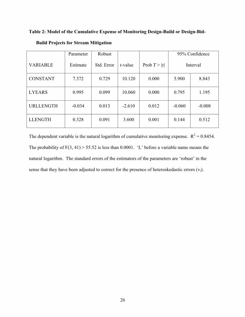
Model of Cumulative Monitoring Expense (Table 2)

The total expense of $46.3 million includes $3.78 million for second-year through fifth-year

monitoring. The figure of $3.78 includes 90 predictions of expense for monitoring in various

years during the four-year period. Although relatively simple, the model used for prediction

accounts for 84.5 percent of the variation in the natural logarithm of cumulative monitoring

expense. Monitoring expense increases, as one would expect, with the number of years during

which EEP has paid or is still under contract to pay for the monitoring. The longer is the actual

length of the restored or enhanced portion of a stream, the larger is the cumulative monitoring

expense. Although cumulative expense increases with stream length, the proportional increase is

less in urban than rural areas. In particular, if the actual length of a restored or enhanced reach is

increased by 1 percent, the cumulative monitoring expense increases, on average, by 0.328

percent if the project is rural and 0.294 percent if the project is urban.

Model of Contractual Expense (Table 5)

The number of stream mitigation units, the location of a project’s site in a developed area,

and the use of priority-three methods to modify the site each has a statistically significant effect

on contractual expense at a five-percent level of confidence. The estimated model accounts for

18

63 percent of the variation in the natural logarithm of contractual expense across the 45 projects.

A one percent increase in stream mitigation units produced by a project in a developed area

induces a 0.778 percent increase, on average, in the contractual expense. A one percent increase

in stream mitigation units of a rural project that is not located in a park or golf course leads to a

0.748 percent increase, on average, in the contractual expense. Similar empirical results occur if,

instead of SMUs, the actual length of the restored or enhanced stream is used as the measure of

project output. If a mitigation project includes a portion of a stream that is enhanced by priority

three, then the project has, on average, 27.0 percent less [= exp(-.315) – 1] contractual expense

than a project that produces credits exclusively through priority one, priority two, or both.

The parameter estimates of the unit costs of two inputs are positive and sum to less than one,

as microeconomic theory predicts. In the sample, a one percent increase in the cost per hour of

labor for engineering and construction management induced, on average, a 0.340 percent

increase in the contractual expense. In the sample, a one percent increase in the cost per gallon

of gasoline led to, on average, a 0.333 percent increase in the contractual expense of a project.

The statistical tests of positive effects of these two input costs are not significant, however.

In the sample, a design-build project would have been 26.7 percent more expensive than a

design-bid-build project, all else equal. However, the test of a positive effect of a design-build

project on contractual expense is significant at only the 15 percent level of confidence.

Discussion of Results

The mitigation fee was $232 per linear foot for the period July 1, 2006 to June 30, 2007. The

inflation-adjusted expense for all projects of $242 per linear foot exceeds this mitigation fee and

also exceeds any inflation-adjusted mitigation fee that EEP has charged in previous fiscal years.

19

Although based on the best available information, the estimates of $46.3 million of total

expense and $242 per linear foot are conservative. Some of the 45 projects might still require

maintenance before monitoring is complete. EEP’s rule-of-thumb for predicting actual expenses

of project administration appears to be conservative because project administration accounted for

only 4 percent of all expenses and was only part of EEP’s overall administration that makes the

in-lieu-fee program for stream mitigation possible.

One important example of unaccounted-for administrative activities pertains to projects that

had been so-called Tier I, II, or III but were permanently stopped before the end of fifth-year

monitoring. EEP officials refer to such projects as Tier 0. The EEP incurred expenses for

gathering information about potential sites, some of which were subsequently deemed unaccept-

able for restoration or enhancement. EEP also incurred expenses to contact and visit landowners,

usually rural ones, who showed interest in placing conservation easements on their riparian land

but who eventually decided against the idea. EEP even incurred expenses, in at least eight

instances (Jurek), for projects that began, i.e., were ‘under production’, but could not be com-

pleted. Some of EEP’s expenses for Tier 0 projects should be allocated to the projects in our

study. Our estimate of project administration expenses omits expense for uncompleted projects.

Economies of scale in monitoring exist. Cumulative monitoring expenses per linear foot of

restored or enhance stream decrease as the length of the monitored stream increase. One pos-

sible reason why cumulative monitoring expenses increase proportionally more at rural sites than

urban ones is that riparian vegetation is usually more abundant and less managed, if at all, at

rural sites. As a result, the monitoring of 100 extra feet of an enhanced or restored stream might

take more time and, thus, be more costly at the rural sites.

Economies of scale exist in both producing stream mitigation units and enhancing or

20

restoring streams. Contractual expense per stream mitigation unit or per linear foot of restored or

enhanced stream decreases proportionately less in developed areas than other areas as the

number of stream mitigation units increases because there are more utility lines and space

constraints in developed areas. Projects that entail priority 3 restoration are less expensive, on

average, because the savings in excavation costs outweigh the extra costs of riprap.

Conclusion

If EEP is to succeed in operating a self-financed, cost-minimizing, non-profit, in-lieu fee

program for stream mitigation in North Carolina, then answers to at least five questions are still

needed. First, how do the costs and quality of full-delivery projects, which were not included in

this analysis, compare to those of design-bid-build projects? Full-delivery projects are those in

which EEP uses mitigation fees to pay a mitigation banker or other firm to take complete

responsibility for a mitigation project. Second, what have been EEP’s expenses for non-

completion of projects, a type of risk? In particular, what were the EEP’s expenses between July

1, 1997 and Aug. 1, 2006 for design-bid-build projects that were terminated before the end of

fifth-year monitoring? To avoid budget shortfalls, EEP must charge a mitigation fee that covers

the costs of non-completion risk. Third, what will be the total maintenance costs of the 45

projects at the end of monitoring? Fourth, how much were EEP’s actual administrative expenses

for the 45 design-bid-build projects? Fifth, how do the estimates of the model of contractual

expense change if, contrary to our assumption in this paper, contractors do not necessarily

succeed at cost minimization? The answer requires estimation of a stochastic cost frontier.

Given the conservatively counted, inflation-adjusted expense of $242 per linear foot for all

projects and given that the EEP must cover all expenses of its in-lieu-fee program for stream

mitigation, fees must increase, project expenses must decrease, or both must occur. Given

21

economies of scale, the EEP could achieve a given amount of mitigation for less expense by

financing fewer projects with longer reaches. The EEP could create a given amount of

mitigation for less expense by financing more projects that are rural and not in parks or golf

courses. The EEP could also generate a given amount of mitigation for less expense by

financing projects that use priority-three methods instead of ones that use only priority one or

two. Other states with in-lieu-fee programs for compensatory mitigation might also use these

results to reduce contractual expenses. However, even if in-lieu-fee programs are managed cost

effectively, people might value the stream mitigation units produced by one long project, by a

project in an undeveloped area, or with priority-three methods differently than they would the

same number of units produced by two short projects, by a project in a developed area, or with

priority-one or priority-two methods. How much their valuations are and might differ are other

important questions for economic research.

Acknowledgements

This research was funded by an EEP contract, award no. D06015, with the University of

North Carolina at Wilmington and subcontract, sub-award no. 503560-06, with Clemson

University. William Sessions, a former graduate student at Clemson University, collected and

entered the data. Melanie Victoria collected information about costs of five projects in the

database of Bernhardt et al. We appreciate the information from and cooperation of numerous

officials at the Ecosystem Enhancement Program: Jeff Jurek, Mac Haupt, Ed Hajnos, Greg

Melia, Stephanie Horton, Sharon Jones, Bill Gilmore, and Suzanne Klimek. Greg Jennings,

Rockie English, and Will Harmon also helped us to learn about the design and implementation of

stream restoration. The views that we have expressed herein are not necessarily those of the EEP

or our colleagues.

22

References

Bernhardt, E. S., M. A. Palmer, J. D. Allan, G. Alexander, K. Barnas, S. Brooks, J. Carr, S.

Clayton, C. Dahm, J. Follstad-Shah, D. Galat, S. Gloss, P. Goodwin, D. Hart, B. Hassett, R.

Jenkinson, S. Katz, G. M. Kondoff, P. S. Lake, R. Lave, J. L. Meyer, T. K. O’Donnell, L.

Pagano, B. Powell, and E. Sudduth. 2005. Policy Forum: Synthesizing U.S. River

Restoration Efforts, Science 38: 636-637, April 29.

BLS. 2006. Producer Price Index, Commodity Data, Finished Goods. Bureau of Labor

Statistics, Department of Commerce, June. http://data.bls.gov/cgi-bin/dsrv?wp

Bonham, J. and K. Stephenson. 2004. A Cost Analysis of Stream Compensatory Mitigation

Projects in the Southern Appalachian Region, paper presented at the American Society of

Agricultural Engineers, Self-Sustaining Solutions for Streams, Watersheds, and Wetlands

Conference, St. Paul Minnesota, September 12-15.

Census Bureau. 2002. Census 2000 Urban and Rural Classification, April 30.

http://www.census.gov/geo/www/ua/ua_2k.html

Davis, Michael L., Robert H. Wayland, III, Jamie Clark, and Scott B. Gudes. Federal Guidance

on the Use of In-Lieu-Fee Arrangements for Compensatory Mitigation under Section 404 of

the Clean Water Act and Section 10 of the Rivers and Harbors Act, October 2001.

http://www.epa.gov/owow/wetlands/pdf/inlieufee.pdf

Doll, Barbara A., Garry L. Grabow, Karen R. Hall, James Halley, William A. Harman, Gregory

D. Jennings, and Dani E. Wise. 2003. Stream Restoration: A Natural Channel Design

Handbook, NC Stream Restoration Institute, NC State University and NC Sea Grant.

http://www.bae.ncsu.edu/programs/extension/wqg/sri/stream_rest_guidebook/

sr_guidebook.pdf

23

EEP. 2007. EEP Strategic Planning, NC Ecosystem Enhancement Program, accessed on June 6.

http://www.nceep.net/services/stratplan/strategicplanning.htm

EEP. 2005. Ecosystem Enhancement Program: 2004-2005 Annual Report. Approved by

William D. Gilmore on Dec. 1. http://www.nceep.net/pages/resources.htm#publications

EEP. 2003. Glossary of Terms related to EEP Watershed Planning. Ecosystem Enhancement

Program, Raleigh NC. http://www.nceep.net/news/reports/watershedplan-glossary.pdf

EIA. 2006. North Carolina Total Gasoline Retail Sales by All Sellers (Cents per Gallon).

Petroleum Navigator, Energy Information Agency, U. S. Department of Energy. December

27. http://tonto.eia.doe.gov/dnav/pet/hist/d100613372m.htm

EPA. 2004. Wetland Regulatory Authority, EPA843-F-04-001, Wetland Fact Sheet Series,

Office of Water, Environmental Protection Agency, Washington DC.

http://www.epa.gov/owow/wetlands/pdf/reg_authority_pr.pdf

EPA. 2003. Wetlands Compensatory Mitigation, EPA843-F-03-002, Office of Wetlands,

Oceans, and Watersheds, Environmental Protection Agency, Washington DC.

http://www.epa.gov/owow/wetlands/pdf/CMitigation.pdf

Gilmore, William D. 2006. Personal communication, Director of the Ecosystem Enhancement

Program, Dept. of the Environment and Natural Resources, Raleigh NC, June.

Jurek, Jeff S. 2006. Personal communication, Director of Project Control and Research for the

Ecosystem Enhancement Program, Dept. of the Environment and Natural Resources, Raleigh

NC, Aug. 22.

Jurek, Jeff S. and D. Mac Haupt. 2004. Analysis of Stream Restoration Costs in North Carolina

Ecosystem Enhancement Program. Conference Proceedings NC SRI Southeastern Regional

Conference on Stream Restoration, NCSU Stream Restoration Institute, NC Sea Grant, and

24

NC Cooperative Extension, Winston-Salem NC, June 21-24, pp. 95-96.

http://www.bae.ncsu.edu/programs/extension/wqg/sri/2004_conference/proceedings.pdf

Ross, Jr., William G., Lyndo Tippett, and Charles R. Alexander, Jr. 2003. Memorandum of

Agreement among the North Carolina Department of Environment and Natural Resources

and the North Carolina Department of Transportation and the United States Army Corps of

Engineers, Wilmington District, July. http://www.nceep.net/images/Final%20MOA.pdf

StataCorp. 2005. Stata Statistical Software: Release 9. College Station, TX: StataCorp LP.

USACE. 2003. Stream Mitigation Guidelines. Wilmington District of the U. S. Army Corps of

Engineers, U. S. Environmental Protection Agency, North Carolina Wildlife Resources

Commission, and Division of Water Quality of North Carolina’s Department of Environment

and Natural Resources, April. http://www.saw.usace.army.mil/wetlands/Mitigation/

Documents/Stream/STREAM%20MITIGATION%20GUIDELINE%20TEXT.pdf

Youngbluth, Terry R. and A. Preston Howard, Jr. 1998. Memorandum of Understanding

between the North Carolina Department of Environment and Natural Resources and the

United States Army Corps of Engineers, Wilmington District, Oct. – Nov.

http://www.nceep.net/images/WRP_MOU.pdf

25

Table 1: Expenses per Design-Build or Design-Bid-Build Project for Stream Mitigation

Type of Expense1 Mean Std. Dev. Minimum Maximum

Project Administration $40,883 $26,773 $10,417 $148,750

Property Rights Acquisition $37,417 $66,610 $0 $346,926

Pre-construction Engineering $146,867 $91,520 $38,092 $490,170

Construction Management $85,152 $46,772 $14,328 $196,002

Construction $539,043 $324,928 $134,492 $1,553,658

Baseline – 1st Year Monitoring $23,847 $16,431 $2,791 $68,614

2nd – 5th Year Monitoring2 $84,073 $20,132 $49,415 $130,911

Past 5th Year Monitoring $3,355 $8,980 $0 $34,320

Maintenance $48,218 $92,660 $0 $351,768

Perpetual Stewardship $21,000 $0 $21,000 $21,000

Total Expenses Per Project $1,029,856 $472,709 $378,766 $2,145,735

Actual Length of Stream

Restored or Enhanced 4,253 2,501 1,400 13,000

1 All expenses of the 4 design-build and 41 design-bid-build projects are in July 2006 dollars.

2 Expenses were observed in 143 and predicted in 90 of the 233 different instances of

monitoring.

26

Table 2: Model of the Cumulative Expense of Monitoring Design-Build or Design-Bid-

Build Projects for Stream Mitigation

VARIABLE

Parameter

Estimate

Robust

Std. Error t-value Prob T > |t|

95% Confidence

Interval

CONSTANT 7.372 0.729 10.120 0.000 5.900 8.843

LYEARS 0.995 0.099 10.060 0.000 0.795 1.195

URLLENGTH -0.034 0.013 -2.610 0.012 -0.060 -0.008

LLENGTH 0.328 0.091 3.600 0.001 0.144 0.512

The dependent variable is the natural logarithm of cumulative monitoring expense. R2 = 0.8454.

The probability of F(3, 41) > 55.52 is less than 0.0001. ‘L’ before a variable name means the

natural logarithm. The standard errors of the estimators of the parameters are ‘robust’ in the

sense that they have been adjusted to correct for the presence of heteroskedastic errors (vi).

27

Table 3: Contractual Expenses per Design-Build or Design-Bid-Build Project and

Determinants of the Expenses (n=45)

Variable Mean Std. Dev. Minimum Maximum

Contractual Expenses1 (CONEXP) $819,280 $425,874 $251,126 $1,956,311

Was the project a design-build one?

(DESBUILD) 0.089 0.288 0 1

Did the project include priority 3

restoration? (PRIOR3) 0.311 0.468 0 1

Was the project site in a golf course,

park, or urban area? (DEVSITE) 0.467 0.505 0 1

Stream Mitigation Units (SMUs) 4,083 2,419 1,400 13,003

Labor cost per hour of pre-construction

engineering and construction

management (ECMWAGE)

$79.75 $8.53 $64.63 $104.39

Retail price of a gallon of gasoline

during construction (GASPRICE) $1.34 $0.27 $0.95 $2.08

1 The sum of expenses in July 2006 dollars for pre-construction engineering, construction

management, construction, and maintenance.

28

Table 4: Total Expenses, Actual Length of Modified Stream, and Expense per Linear Foot

of Design-Build and Design-Bid-Build Projects for Stream Mitigation by Location

Variable All Projects (n=45) Urban Projects Rural Projects

Total Expenses (July 2006 $s) $46,343,525 $18,338,967 $28,004,558

Actual Length (ft.) of Restoration

or Enhancement 191,374 64,347 127,027

Expense per Actual Linear Foot $242.16 $285.00 $220.46

29

Table 5: Model of the EEP’s Contractual Expense of a Design-Build or Design-Bid-Build

Project (n=45) for Stream Mitigation

VARIABLE Estimate Std. Error t-value Prob T > |t| 95% Confidence Interval

Constant 5.764 2.368 2.430 0.020 0.970 10.559

DESBUILD 0.237 0.199 1.190 0.241 -0.166 0.639

PRIOR3 -0.315 0.136 -2.320 0.026 -0.590 -0.040

DEVSLSMU 0.030 0.014 2.100 0.042 0.001 0.059

LSMU 0.748 0.106 7.050 0.000 0.533 0.963

LECMWAGE 0.340 0.527 0.640 0.523 -0.727 1.407

LGASPRICE 0.333 0.316 1.050 0.299 -0.307 0.973

The dependent variable is the natural logarithm of expenses for pre-construction engineering,

construction management, construction, and maintenance. R2 = 0.632. The probability of F(6,

38) > 10.87 is less than 0.0001. ‘L’ before a variable name means the natural logarithm.