Estimating Wind Velocities in Atmospheric Mountain Waves ...
220
Ni Zhang Department of Electrical and Computer Engineering A thesis presented for the degree of Doctor of Philosophy University of Canterbury Christchurch, New Zealand October 2012
Transcript of Estimating Wind Velocities in Atmospheric Mountain Waves ...

Estimating Wind Velocities in
Atmospheric Mountain Waves Using
Sailplane Flight Data
Ni Zhang
Department of Electrical and Computer Engineering
A thesis presented for the degree ofDoctor of Philosophy
University of CanterburyChristchurch, New Zealand
October 2012


TO MY LOVING PARENTS

iv

Contents
Contents v
1 Introduction 1
1.1 The Atmosphere . . . . . . . . . . . . . . . . . . . . . . . . . . . . . . . . . . . 1
1.1.1 Pressure and temperature versus altitude . . . . . . . . . . . . . . . . 1
1.1.2 Moisture in the atmosphere . . . . . . . . . . . . . . . . . . . . . . . . 4
1.1.3 Adiabatic lapse rate . . . . . . . . . . . . . . . . . . . . . . . . . . . . 5
1.1.4 Potential temperature . . . . . . . . . . . . . . . . . . . . . . . . . . . 7
1.1.5 Virtual temperature and virtual potential temperature . . . . . . . . 7
1.1.6 Stability of the atmosphere . . . . . . . . . . . . . . . . . . . . . . . . 8
1.2 Mountain lee waves . . . . . . . . . . . . . . . . . . . . . . . . . . . . . . . . . 11
1.2.1 Linear mountain wave theory . . . . . . . . . . . . . . . . . . . . . . . 15
1.2.2 Homogeneous atmosphere . . . . . . . . . . . . . . . . . . . . . . . . 17
1.2.3 Trapped lee waves . . . . . . . . . . . . . . . . . . . . . . . . . . . . . 18
1.3 Sailplanes . . . . . . . . . . . . . . . . . . . . . . . . . . . . . . . . . . . . . . 21
1.3.1 Sailplane maneuvers and controls . . . . . . . . . . . . . . . . . . . . 21
1.3.2 Sailplane aerodynamics - steady flight . . . . . . . . . . . . . . . . . . 22
1.3.3 Sailplane aerodynamics - turning flight . . . . . . . . . . . . . . . . . 25
1.3.4 Sailplane performance . . . . . . . . . . . . . . . . . . . . . . . . . . . 27
1.3.5 Sailplane instruments . . . . . . . . . . . . . . . . . . . . . . . . . . . 31
v

vi Contents
1.4 Inverse problems and Bayesian inference . . . . . . . . . . . . . . . . . . . . 34
1.4.1 Data matching . . . . . . . . . . . . . . . . . . . . . . . . . . . . . . . 35
1.4.2 Regularization . . . . . . . . . . . . . . . . . . . . . . . . . . . . . . . 35
1.4.3 Likelihood methods . . . . . . . . . . . . . . . . . . . . . . . . . . . . 35
1.4.4 Bayesian methods . . . . . . . . . . . . . . . . . . . . . . . . . . . . . 36
1.5 Previous work on wind velocity estimation from aircraft flight data . . . . . 38
2 Problem Characteristics 41
2.1 The 3D problem . . . . . . . . . . . . . . . . . . . . . . . . . . . . . . . . . . . 41
2.2 The horizontal (2D) problem . . . . . . . . . . . . . . . . . . . . . . . . . . . . 42
2.2.1 Case 1: Ground velocity, airspeed and heading . . . . . . . . . . . . . 45
2.2.2 Case 2: Ground velocity and airspeed . . . . . . . . . . . . . . . . . . 45
2.2.3 Case 3: Ground velocity and heading . . . . . . . . . . . . . . . . . . 52
2.2.4 Case 4: Ground velocity data only . . . . . . . . . . . . . . . . . . . . 55
2.2.5 Effect of wind velocity variation . . . . . . . . . . . . . . . . . . . . . 60
2.3 The vertical problem . . . . . . . . . . . . . . . . . . . . . . . . . . . . . . . . 62
2.4 Summary . . . . . . . . . . . . . . . . . . . . . . . . . . . . . . . . . . . . . . . 63
3 Flight Data 65
3.1 The Perlan project . . . . . . . . . . . . . . . . . . . . . . . . . . . . . . . . . . 65
3.2 Flight 1: Perlan Flight 39 Southern California . . . . . . . . . . . . . . . . . . 67
3.3 Flight 2: Perlan Flight 63: Argentina . . . . . . . . . . . . . . . . . . . . . . . 73
3.4 Flight 3: Perlan Flight 66: Argentina . . . . . . . . . . . . . . . . . . . . . . . 78
3.5 Flight 4: Perlan Flight 24: Omarama . . . . . . . . . . . . . . . . . . . . . . . 83
3.6 Airspeed correction . . . . . . . . . . . . . . . . . . . . . . . . . . . . . . . . . 88
4 A Heuristic Method for Estimating 3D Wind Velocities 91
4.1 Horizontal wind velocity estimate . . . . . . . . . . . . . . . . . . . . . . . . 91

Contents vii
4.2 Vertical wind speed estimate . . . . . . . . . . . . . . . . . . . . . . . . . . . 95
4.3 Results . . . . . . . . . . . . . . . . . . . . . . . . . . . . . . . . . . . . . . . . 96
4.3.1 Flight 1: Perlan Flight 39: California . . . . . . . . . . . . . . . . . . . 96
4.3.2 Flight 2: Perlan Flight 63: Argentina . . . . . . . . . . . . . . . . . . . 109
4.3.3 Flight 3: Perlan Flight 66: Argentina . . . . . . . . . . . . . . . . . . . 115
4.3.4 Flight 4: Perlan Flight 24: Omarama . . . . . . . . . . . . . . . . . . . 122
5 Flight Simulation 129
6 Maximum Likelihood Estimation 137
6.1 Introduction . . . . . . . . . . . . . . . . . . . . . . . . . . . . . . . . . . . . . 137
6.2 Measurement model . . . . . . . . . . . . . . . . . . . . . . . . . . . . . . . . 138
6.3 Position, airspeed and heading data . . . . . . . . . . . . . . . . . . . . . . . 140
6.3.1 Methods . . . . . . . . . . . . . . . . . . . . . . . . . . . . . . . . . . . 140
6.3.2 Simulation results . . . . . . . . . . . . . . . . . . . . . . . . . . . . . 141
6.4 Position and airspeed data . . . . . . . . . . . . . . . . . . . . . . . . . . . . . 146
6.4.1 Methods . . . . . . . . . . . . . . . . . . . . . . . . . . . . . . . . . . . 146
6.4.2 Simulation results . . . . . . . . . . . . . . . . . . . . . . . . . . . . . 146
6.4.3 Experimental results . . . . . . . . . . . . . . . . . . . . . . . . . . . . 149
6.5 Position and heading data . . . . . . . . . . . . . . . . . . . . . . . . . . . . . 153
6.5.1 Method . . . . . . . . . . . . . . . . . . . . . . . . . . . . . . . . . . . . 153
6.5.2 Simulation results . . . . . . . . . . . . . . . . . . . . . . . . . . . . . 153
6.5.3 Experimental results . . . . . . . . . . . . . . . . . . . . . . . . . . . . 154
6.6 Discussion . . . . . . . . . . . . . . . . . . . . . . . . . . . . . . . . . . . . . . 156
7 Maximum a posteriori Estimation 159
7.1 Introduction . . . . . . . . . . . . . . . . . . . . . . . . . . . . . . . . . . . . . 159
7.2 Prior models for sailplane air velocity . . . . . . . . . . . . . . . . . . . . . . 161
7.3 Maximum a posteriori estimator . . . . . . . . . . . . . . . . . . . . . . . . . 165

viii Contents
7.4 2D simulation results . . . . . . . . . . . . . . . . . . . . . . . . . . . . . . . . 169
7.4.1 Simulations 1 and 2 . . . . . . . . . . . . . . . . . . . . . . . . . . . . . 171
7.4.2 Simulations 3 and 4 . . . . . . . . . . . . . . . . . . . . . . . . . . . . . 174
7.4.3 Simulation 5 . . . . . . . . . . . . . . . . . . . . . . . . . . . . . . . . . 175
7.4.4 Simulation 6 . . . . . . . . . . . . . . . . . . . . . . . . . . . . . . . . . 177
7.4.5 Simulation 7 . . . . . . . . . . . . . . . . . . . . . . . . . . . . . . . . . 180
7.5 3D simulation results . . . . . . . . . . . . . . . . . . . . . . . . . . . . . . . . 182
7.6 Experimental results . . . . . . . . . . . . . . . . . . . . . . . . . . . . . . . . 188
7.7 Discussion . . . . . . . . . . . . . . . . . . . . . . . . . . . . . . . . . . . . . . 193
8 Conclusions 195

Abstract
Atmospheric mountain waves form in the lee of mountainous terrain under appropriateconditions of the vertical structure of wind speed and atmospheric stability. Trapped leewaves can extend hundreds of kilometers downwind from the mountain range, and theycan extend tens of kilometers vertically into the stratosphere. Mountain waves are of im-portance in meteorology as they affect the general circulation of the atmosphere, can influ-ence the vertical structure of wind speed and temperature fields, produce turbulence anddowndrafts that can be an aviation hazard, and affect the vertical transport of aerosols andtrace gasses, and ozone concentration.
Sailplane pilots make extensive use of mountain lee waves as a source of energy withwhich to climb. There are many sailplane wave flights conducted every year through-out the world and they frequently cover large distances and reach high altitudes. Modernsailplanes frequently carry flight recorders that record their position at regular intervalsduring the flight. There is therefore potential to use this recorded data to determine the 3Dwind velocity at positions on the sailplane flight path. This would provide an additionalsource of information on mountain waves to supplement other measurement techniquesthat might be useful for studies on mountain waves. The recorded data are limited how-ever, and determination of wind velocities is not straightforward.
This thesis is concerned with the development and application of techniques to determinethe vector wind field in atmospheric mountain waves using the limited flight data col-lected during sailplane flights. A detailed study is made of the characteristics, uniqueness,and sensitivity to errors in the data, of the problem of estimating the wind velocities fromlimited flight data consisting of ground velocities, possibly supplemented by air speedor heading data. A heuristic algorithm is developed for estimating 3D wind velocities inmountain waves from ground velocity and air speed data, and the algorithm is applied toflight data collected during “Perlan Project” flights. The problem is then posed as a sta-tistical estimation problem and maximum likelihood and maximum a posteriori estimatorsare developed for a variety of different kinds of flight data. These estimators are tested onsimulated flight data and data from Perlan Project flights.
ix

x

Acknowledgements
I would like to express my gratitude to my supervisor Prof. Rick Millane. Without his con-stant guidance and encouragement, this thesis would not have been possible. My specialthanks also go to my co-supervisor Dr. Allan McInnes and Dr. Peter Smith. They haveprovided valuable suggestions for the research. I am also grateful to Prof Phil Bones andDr Steve Weddell for their advice and encouragement. I am grateful to the NZ TertiaryEducation Commission for award of Top Achiever Doctoral scholarship.
I would like to extend my appreciation to Einar Enevoldson, formally of NASA DrydenFlight Research Centre and Jim Murray of NASA Dryden Flight Research Centre. Einarand Jim provided the flight data described in Chapter 3 and have been the source of muchuseful information and advice. NASA Dryden also provided support in terms of instru-mentation for these flights as well as helping with some publication costs. Dr. ElizabethAustin also provided advice and encouragement. Einar also piloted, together with SteveFossett, the flights described in Chapter 3. The Perlan Project flights were supported finan-cially by Steve before his untimely death in 2007.
Many thanks to my colleagues and friends in the Computational Imaging Group and therest of the Department for their assistance and companionship, especially Victor Lo, DavidWojtas, Bing Wu, Bahar Dar, Yu-An Chen, Michael Hwang and Tri Pham Minh. Thanks tomy supportive flatmates and friends Maung Shein, Brian Peng, Ysabel Legaspi, Tiffany Su,and Nancy Xu.
Last but not least, it is my parents who have supported me the most throughout my up-bringing and education. To my mother Li Kun and father Zhang Yongsheng, I cannot thankyou enough.
xi

xii

Preface
This thesis is concerned with the development and application of techniques to use limitedflight data collected during sailplane flights to determine the vector wind field in atmo-spheric mountain waves. The thesis can be divided into three topics. (1) A study of thecharacteristics, uniqueness and sensitivity to errors in the data, of the problem of estimat-ing the wind velocities from limited flight data. (2) A heuristic method for determining3D wind velocities from ground velocity and airspeed data, and application to data fromsailplane wave flights. (3) Statistical estimation of wind velocities from a number of dif-ferent kinds of limited flight data using maximum likelihood and maximum a posterioriestimation, and application to simulated and actual flight data. Review material is pre-sented in Chapter 1, and original work is presented in Chapters 2-7.
Some of the work presented here builds on work developed by some of the author’s pre-decessors. The bulk of this prior work is described in [1]. This includes the following:Approximately 25% of the work presented in Section 2.2.2. The basic ideas of Section 4.1and 4.2, although the author has refined these ideas and their implementation and coding.Approximately 20% of the results presented in Section 4.3.1.
Chapter 1 contains a review of background material including relevant atmospheric physics,lee waves, sailplane aerodynamics and flight behavior, and inverse problems.
Chapter 2 contains an analysis of uniqueness and sensitivity of determining wind velocitiesfrom flight data consisting of ground velocity with airspeed or heading, or ground velocityalone.
Chapter 3 summarises the four flights for which experimental data is used in the thesis.
Chapter 4 describes a heuristic method of estimating the 3D wind velocities from groundvelocity and airspeed data. The method is applied to the above four flights.
Chapter 5 describes methods used to generate simulated flight data.
Chapter 6 describes the application of maximum likelihood estimation to the problem ofestimating wind velocities from ground velocity with airspeed or heading data. The meth-ods are applied to simulated data and to actual flight data.
xiii

xiv Contents
Chapter 7 considers the problem of wind velocity estimation when only ground velocitydata are available. Suitable prior models for the airspeed and heading are considered.Maximum a posteriori estimators are developed. These estimators are applied to simulatedand actual flight data.
A summary of key results from this thesis and suggestions for future research are given inChapter 8.
Aspects of the work presented in this thesis have been published and presented. They arelisted here in order of presentation.
Zhang, N., Millane, R.P., Hunter, A.J., (2009) Estimating 3D wind fields in mountain wavesusing sailplane flight data. Auckland, New Zealand: New Zealand Marine Science Societyand Meteorological Society Joint Conference, 2-4 September 2009.
Zhang, N., Millane, R.P. and Hunter, A.J. (2010) Estimating wind velocity from limited air-craft flight data. Wuhan, China: 2010 2nd International Conference on Industrial Mecha-tronics and Automation (ICIMA), 30-31 May 2010. In Proceedings 626-629.
Zhang, N., Millane, R.P. and Hunter, A.J. (2010) In situ determination of wind fields fromsailplane flight data. San Diego, CA, USA: In “Image Reconstruction from Incomplete DataVI,” P.J. Bones, M.A. Fiddy and R.P. Millane (Eds.), Proc. SPIE, Vol. 7800, 78000A/1-6, 2010.
Millane, R.P., Stirling, G.D., Brown, R.G., Zhang, N., Lo, V.L., Enevoldson, E. and Murray,J.E. (2010) Estimating Wind Velocities in Mountain Lee Waves Using Sailplane Flight Data.Journal of Atmospheric and Oceanic Technology 27(1): 147-158.
Zhang, N., Millane, R.P., Enevoldson, E. and Murray, J.E. (2010) Measuring 3D Wind Fieldsin Mountain Waves Using Sailplane Flight Data. Szeged, Hungary: XXX OSTIV Congress,28 July 4 August 2010.
Zhang, N., Millane, R.P., Enevoldson, E. and Murray, J.E. (2010) Measuring 3D Wind Fieldsin Mountain Waves Using Sailplane Flight Data. Technical Soaring 36(2): 57-66.
Zhang, N., Millane, R.P., Hunter, A.J., Enevoldson, E. and Murray, J.E. (2011) Estimatingwind velocities from limited sailplane flight data. Dallas, Texas: 13th International Asso-ciation of Science and Technology for Development (IASTED) International Conference onImage and Signal Processing, 14-16 Dec 2011. In Proc. IASTED Signal and Image Process-ing 2011, 109-114.
Zhang, N., Millane, R.P., Enevoldson, E. and Murray, J.E. (2012) Determining wind fields inmountain waves using sailplane flight data. San Diego, CA, USA: In “Image Reconstruc-tion from Incomplete Data VII,” P.J. Bones, M.A. Fiddy and R.P. Millane (Eds.), Proc. SPIE,Vol. 8500, 85000S/1-9, 2012.

Contents xv
Zhang, N., Millane, R.P., Enevoldson, E. and Murray, J.E. (2012) Estimating wind velocitiesfrom limited sailplane flight data. Texas USA: XXXI OSTIV Congress, 8-15 August 2012.
Zhang, N., Millane, R.P., Enevoldson, E. and Murray, J.E. (2012) Mountain wave 3D windfields from sailplane flight data. Wellington, New Zealand: New Zealand MeteorologicalSociety Annual Conference, 19-20 November 2012.

xvi

Chapter 1
Introduction
1.1 The Atmosphere
The state of the atmosphere is defined by the fundamental parameters temperature, den-sity, pressure and humidity. Dry air behaves almost as an ideal gas, which is governed bythe ideal gas law
PV = nRT, (1.1)
where P is the pressure, V is the volume of gas, n is the number of moles of gas, R =
8.31432 JK−1mol−1 is the universal gas constant, and T is the absolute temperature.
1.1.1 Pressure and temperature versus altitude
Standard atmosphere models are defined using a representative vertical distribution ofatmospheric parameters. These standard conditions are the basis for most aircraft perfor-mance data, and are used for calibration of aircraft flight instruments. A commonly-usedmodel is the International Standard Atmosphere (ISA), which defines a standard atmo-spheric pressure of 1013.2 millibars and a temperature of 288◦K (15◦C) at sea level [2].According to the temperature change with increasing altitude, the earth’s atmosphere is di-vided into 4 layers, namely the troposphere, stratosphere, mesosphere and thermosphere.The boundaries between the layers are called the tropopause, stratopause, and mesopause.The standard atmosphere model assumes a dry atmosphere for which the ideal gas law andhydrostatic equation apply. The pressure, temperature, density, and speed of sound pro-files for the standard atmosphere model are shown in Fig. 1.1. The pressure and densitydecrease exponentially with altitude, however the temperature can decrease, increase withaltitude or stay constant in different layers. Most weather phenomena occur in the tro-posphere since this layer contains most of the water vapor and clouds. The lower part ofthe troposphere interacts with the land and sea surface, and produces thermals, mountainwaves and sea-breeze fronts. Sailplanes are usually flown in the troposphere, and havealso been flown into the lower stratosphere with lift provided by mountain waves.
1

2 Introduction
Figure 1.1 US standard atmosphere model: temperature, pressure, density and speed of soundversus altitude [2].
The relationships between temperature, density and pressure in the atmosphere are de-rived as follows. Consider a small column of air with unit horizontal cross-section area asshown in Fig. 1.2 between height z and z+dz. The pressure exerted on the bottom and thetop of the air column surface is P + dP and P , respectively. The mass of the air betweenz and z + dz in the column of air is dm = ρdz where ρ is the density of the air. The forceon the column due to gravity is gdm = gρdz where g is the acceleration due to gravity. Athydrostatic equilibrium, the force acting on the air column due to the pressure differencedP = P (z + dz) − P (z) is equal and opposite to the force due to gravity, i.e. dP = −gρdz.This gives the hydrostatic equation
dP
dz= −gρ. (1.2)
The air density is given byρ =
nm0
V, (1.3)
where m0 = 0.02896 kg/mol is the mean molar mass of air and V is the volume. Using the

1.1 The Atmosphere 3
z+dz
z
P(z+dz)
P(z)
unit area
Figure 1.2 A column of air between height z and z + dz with unit horizontal cross-sectional area.
ideal gas law (1.1) and (1.3) givesP = ρRdT, (1.4)
where Rd = R/m0 = 287.053 Jkg−1K−1 is the specific gas constant for dry air, i.e. the gasconstant normalised by the molar mass of dry air. Substituting (1.4) into (1.2) gives
dP
dz= − gP
RdT. (1.5)
The lapse rate Γ(z) is defined as the rate of change of temperature with altitude, i.e.
Γ(z) =dT
dz. (1.6)
Consider first the case when the temperature is constant, i.e. Γ(z) = 0, and T = T0, whereT0 is the temperature at a reference altitude z0. This applies in the lower stratospherebetween an altitude of about 11 and 20 km. From (1.5),
dP
P= − g
Rd
dz
T0, (1.7)
and integrating both sides gives
log
(P
P0
)= − g
RdT0(z − z0), (1.8)
where P0 is the pressure at altitude z0. The pressure therefore decreases exponentially withaltitude, i.e.
P = P0 exp
(− g
RdT0(z − z0)
). (1.9)

4 Introduction
Consider now the case where the temperature changes linearly with altitude, i.e. Γ is con-stant and non-zero, and dT = Γdz. Substitution into (1.5) gives
dP
P= − g
RdΓ
dT
T. (1.10)
Integrating (1.10) gives
log
(P
P0
)= − g
RdΓlog
(T
T0
), (1.11)
where P0 is the pressure at altitude z0, so that
P
P0=
(T
T0
)α
, (1.12)
where α = −g/RdΓ. The temperature is given by T = T0 + Γ(z − z0) so that
P = P0
(1 + (z − z0)
Γ
T0
)α
, (1.13)
which gives the pressure as a function of altitude. Taking z0 as the altitude at sea level anddefining z1 as altitude above sea level, then
P = P0
(1 +
Γz1T0
)α
. (1.14)
1.1.2 Moisture in the atmosphere
The air density is affected by the amount of water vapor in the air. This is because themolecular weight of water vapor (18.0153 g/mol) is lower than that of the majority of thegases in the air (predominately nitrogen at 28.0134 g/mol and oxygen at 31.9989 g/mol).The amount of water vapor that air can sustain is affected by the temperature. Warm aircan hold more moisture than dry air. The (mass) mixing ratio, r, is defined as the massof water vapor contained in a unit mass of air, and can also be written in terms of partialpressures as
r =εe
P, (1.15)
where ε is the ratio of specific gas constant of dry air to that of water vapor, ε = Rd/Rv =
0.622, Rv is the specific gas constant for water vapor, and e is the partial pressure of thewater vapor. The subscripts v and d denote water vapor and dry air, respectively. Air issaid to be saturated when the liquid water and vapor contained in the air are at equilibriumat a certain temperature. The partial pressure of water vapor at saturation at temperatureT is denoted es(T ). The mixing ratio at saturation rs is then
rs =εes(T )
P. (1.16)

1.1 The Atmosphere 5
The energy per unit mass required to change a substance from one state to another is calledthe latent heat L. At the transition from liquid water to water vapor the amount of heatabsorbed per unit mass of water is called the latent heat of vaporization, Lv. The variationof the partial pressure of water vapor in saturated air es with respect to temperature isgiven by the Clausius-Clapeyron equation [3]
desdT
=Lv
TdV, (1.17)
where dV is the increase of volume as a unit mass of water changes from liquid to vapor.Since the volume of the water vapor is much greater than that of the liquid, dV is approx-imately equal to the volume of water vapor per unit mass Vv. Using the ideal gas law, forunit mass of water vapor,
dV = Vv =1
ρv=
RvT
es, (1.18)
where ρv is the density of water vapor and T is the temperature at the phase transition.Substituting (1.18) in (1.17) gives
desdT
=LvesRvT 2
(1.19)
which is an alternative form of the Clausius-Clapeyron equation with volume eliminated.
Another important measure of the moisture content of air is the relative humidity (RH),defined as the ratio of the partial pressure of water vapor in the air to that of water vaporin saturated air, i.e.
RH =e
es=
r
rs. (1.20)
Dry air has a RH of 0% and saturated air a RH of 100%.
1.1.3 Adiabatic lapse rate
The effects of vertical movement of air in the atmosphere are conveniently analysed us-ing the concept of an “air parcel.” An air parcel can be imagined as a small mass of airwhose passage through the environment can be traced. It is influenced by the environ-ment but does not influence the environment. The pressure in the parcel is equal to thatof the environment but its temperature, density, etc. may differ from the environment.Vertical movement of an air parcel with no heat transfer between the air parcel and theambient atmosphere, is called an adiabatic process. Assuming dry or unsaturated air, thedry adiabatic lapse rate is derived as follows.
Consider an air parcel of unit mass rising adiabatically from height z to z + dz. The workperformed on the air parcel is, using (1.2),
dW = V dP = −gdz. (1.21)

6 Introduction
The change in the enthalpy, the total energy, of the air parcel dH is given by
dH = cpdT = cpΓ(z)dz, (1.22)
where cp is the specific heat capacity of air at constant pressure, cp = 1.0 × 10³ Jkg−1K−1.For an adiabatic process, dH = dW so that from (1.21) and (1.22),
Γd(z) = − g
cp, (1.23)
i.e. Γd is constant (independent of altitude) and Γd = −9.8 K/km. The negative sign isexpected since as the air rises, it expands and cools. This applies to moist unsaturatedair also since the moisture content gives little change to the specific heat. The relation-ships between pressure, temperature and altitude for Γ constant derived in Section 1.1.1are therefore of particular importance. If the troposphere were in perfect adiabatic equi-librium then the lapse rate would be Γd. However, the adiabatic equilibrium is imperfect(i.e. conduction effects are present), the troposphere tends to be more isothermal, and thetypical, or environmental, lapse rate Γ is about -5 K/km [4].
For saturated air, the lapse rate decreases (i.e. is less negative) since condensation of watervapor (as the temperature decreases) releases latent heat that warms the air as it rises.When a saturated air parcel rices, the heat released to the parcel due to condensation perunit mass of air is [3]
dQ = −Lvdrs. (1.24)
The total heat transferred to the rising air parcel is then
cpdT + gdz + Lvdrs = 0. (1.25)
Taking the logarithm of (1.16) and differentiating gives
drsrs
=deses
− dP
P. (1.26)
Using (1.5) and (1.19) and substituting in the RHS of (1.26) gives
drsrs
=LvdT
RvT 2+
gdz
RdT. (1.27)
Substituting for drs from (1.27) into (1.25) gives(cp +
L2vrs
RvT 2
)dT + g
(1 +
LvrsRdT
)dz = 0, (1.28)
and the saturated adiabatic lapse rate is given by
Γs =dT
dz=
(− g
cp
)(1 + (Lvrs)/(RdT ))
(1 + (L2vrs)/(cpRvT 2))
. (1.29)

1.1 The Atmosphere 7
As rs is a function of temperature and pressure, Γs is also a function of temperature andpressure and can be written in the form Γs = Γdf(T, P ) and f(T, P ) < 1. Since the tem-perature and pressure depend on altitude, Γs generally varies with altitude. Γs is typically-4 K/km near the surface, and -(6-7) K/km in the middle of the troposphere [4]. At highaltitudes where the air is colder and holds less water vapor, Γs nearly equals Γd. Note thatif the latent heat Lv were zero then Γs would equal Γd as expected. Γs is dependent ontemperature in such a way that the lower the temperature, the less moisture the air holdsand the closer Γs is to Γd. When a moist air parcel rises, it cools dry adiabatically followingthe dry adiabat with a constant potential temperature until it reaches a RH of 100% (this iscalled the lifting condensation level (LCL)) and it then follows the saturated adiabat withany further lifting.
1.1.4 Potential temperature
Potential temperature θ is a quantity related to temperature that is defined to remove theeffects of dry adiabatic temperature changes. By definition, θ is the temperature that an airparcel at pressure P would acquire if adiabatically brought to a standard reference pressureor altitude.
The potential temperature as as a function of altitude is then simply
θ(z) = T (z)− Γdz, (1.30)
where the reference altitude is at z = 0. If the reference pressure is denoted P0, then using(1.12) and (1.23) shows that the potential temperature can be written in terms of pressureas
θ(P ) = T (P )
(P0
P
)Rd/cp
. (1.31)
For an adiabatically displaced air parcel the potential temperature is constant, i.e. dθ/dz =
0.
1.1.5 Virtual temperature and virtual potential temperature
A virtual temperature Tv is defined to include the buoyant effect of water vapor and liquidwater in the air. Virtual temperature is the temperature dry air must have to have a densityequal to the density of moist air at the same pressure. Since water vapor is less densethan dry air, moist unsaturated air is more buoyant than dry air at the same temperature.Therefore, the virtual temperature of unsaturated moist air is always greater than the actualair temperature. The density of liquid water is greater than that of dry air, thus cloudy(saturated) air is less buoyant than cloud-free air at the same temperature. The ideal gaslaw (1.4) can be written for moist air in terms of virtual temperature as
P = ρRdTv. (1.32)

8 Introduction
The pressure is given byP = Pd + e, (1.33)
where Pd denotes the partial pressure of the dry air and
ρ = ρd + ρv =Pd
RdT+
e
RvT=
P − e
RdT+
e
RvT. (1.34)
Substituting (1.34) into (1.32) and using (1.15) gives
P =(εer
− e+ εe) Tv
T=
εe
r, (1.35)
and simplifying givesTv
T=
(1−
(1
ε− 1
)r
)−1
, (1.36)
and expanding to first order in r and substituting ε = 0.622 gives
Tv = T
(1 +
(1
ε− 1
)r
)= T (1 + 0.61r). (1.37)
For saturated air, the liquid water contained in the air due to condensation needs to betaken into consideration, and the virtual temperature is given by
Tv = T (1 + 0.61rs − rL), (1.38)
where rL is the mixing ratio of liquid water. In the same context, the virtual potentialtemperature for moist air is given by
θv = θ(1 + 0.61r), (1.39)
and for saturated air byθv = θ(1 + 0.61rs − rL). (1.40)
1.1.6 Stability of the atmosphere
Stability is a measure of the gravitational resistance of the atmosphere to vertical displace-ments. A region of the atmosphere is said to be statically stable if a vertically-displacedair parcel in this region tends to return to its equilibrium position. The restoring force thatbrings the air parcel back to equilibrium is a buoyancy force and is a result of the differencein density between the air parcel and the air into which it moves. The stability dependson the difference between the adiabatic and environmental lapse rates. This can be seenin Fig. 1.3 by considering an air parcel at the cross-over point. If Γ < Γd, then a parceldisplaced upwards is colder and therefore heavier than the surroundings and has a ten-dency to fall back to its original position and the atmosphere is statically stable. A parceldisplaced downwards will be lighter and will also tend to return to its original position. IfΓ > Γd the environmental temperature falls more rapidly with height than the dry adia-

1.1 The Atmosphere 9
Unstable
Stable
Γd
T
z
Γ < Γd
Γ > Γd
z0
Figure 1.3 Illustration of stability of the atmosphere using the temperature profile. The dashedlines indicate environmental lapse rates, and the solid line indicates the dry adiabatic lapse rate.
batic lapse rate and a parcel displaced upwards is lighter than the surroundings and willcontinue to rise, and the atmosphere is statically unstable. If Γ = Γd the atmosphere issaid to be neutrally stable. For saturated air the same applies with Γd replaced by Γs. IfΓs < Γ < Γd, a saturated parcel is unstable and an unsaturated parcel is stable, and theatmosphere is sometimes called conditionally stable.
In a stability stable region, the restoring force causes the air parcel to oscillate about therest position and eventually back to the equilibrium. Consider an air parcel with volumeV in a statically stable environment originally at the equilibrium height z0 with density ρ0,displaced by a small increment in height dz. The density of the environment is a function ofaltitude, ρ(z). The buoyancy force is equal to the weight of air displaced by the air parcel,given by
F = −gV dρ = −kdz, (1.41)
where dρ = ρ(z)− ρ0, the difference between the density of the air parcel and the environ-ment, and k = gV dρ/dz. The negative sign is a result of, for example, if dρ is positive thenthe air parcel is denser (‘heavier’) than the environment and the restoring force is down(-ve z). Since the restoring force is proportional to, and is the opposite direction to (assum-ing that dρ/dz is positive), the displacement, the air parcel is a simple harmonic oscillatorwith spring constant k. Newton’s third law for the air parcel is then
−kdz = ρ0Vd2(dz)
dt2. (1.42)

10 Introduction
Denoting the displacement of the air parcel by zρ, (1.42) becomes
d2zρdt2
+
(k
ρ0V
)zρ = 0 (1.43)
which has solutionzρ(t) = A cos(ω0t+ ϕ), (1.44)
where A is the amplitude, ϕ is a phase shift, and ω0 is the natural frequency of the harmonicmotion given by
ω0 =
(k
ρ0V
)1/2
=
(g
ρ0
dρ(z)
dz
)1/2
. (1.45)
In meteorology, ω0 is called the buoyancy, or Brunt-Vaisala frequency, and is equal to about0.01 s−1 for average tropospheric conditions [5]. In meteorology, the buoyancy frequencyis usually denoted N , but the notation ω0 will be used here to emphasize that it is a naturalfrequency of the system. It can also be shown that the buoyancy frequency is related to thepotential temperature by [6]
ω20 =
g
θ
dθ
dz. (1.46)
For saturated air, the same applies with the potential temperature replaced by the virtualpotential temperature.
The static stability, denoted S, of a region of the atmosphere is defined by
S = ω20. (1.47)
If ω0 is real then S > 0 and the atmosphere is statically stable. If ω0 is imaginary, thesolution to (1.43) has exponential growth, S < 0 and the region is unstable.
Static stability depends on the difference between the environmental and adiabatic lapserates, and can be quantified as follows. The density difference dρ in the above analysis hastwo components, one due to the change in density of the air parcel as it rises (assumed dryadiabatically) and one due to the change in the density of the environment with altitude.Consider an unsaturated air parcel originally at height z0, with values of temperature T0,pressure P0 and density ρ0 all equal to its surroundings. If the parcel is adiabatically dis-placed to z1 = z0 + dz, its temperature is increased to Tp1 = T0 + Γddz. The temperatureof the environment at z1 is Te1 = T0 + Γdz where Γ is the environmental lapse rate. Thepressures inside and outside the parcel at z1 are equal, i.e. Pe1 = Pp1 = P1. Referring to(1.4), the density difference is then

1.2 Mountain lee waves 11
dρ =P1
Rd
(1
Tp1− 1
Te1
)=
P1
Rd
((T0 + Γddz)
−1 − (T0 + Γdz)−1)
=P1
RdT0
((1 +
Γd
T0dz
)−1
−(1 +
Γ
T0dz
)−1). (1.48)
As Γddz and Γdz are small, the first order Binomial expansion of (1.48) is
dρ ≈ P1
RdT0
(1− Γd
T0dz − 1 +
Γ
T0dz
)=
P1
RdT20
(Γ− Γd)dz, (1.49)
and substituting into (1.45) gives
ω0 =
(g
T0(Γ− Γd)
)1/2
, (1.50)
i.e. the buoyancy frequency is a function of the difference between the environmental andadiabatic lapse rates.
1.2 Mountain lee waves
Mountain lee waves are a type of atmospheric gravity wave (AGW) that are generatedby stratified flow over mountains. AGWs are an oscillation arising from buoyancy, as de-scribed in Section 1.1.6. In a stable stratified atmosphere the buoyancy is continuouslydistributed, and if the air is disturbed from equilibrium, the buoyancy force tends to re-store any displacement which then causes the oscillation [7]. AGWs can propagate up toaltitudes of 100 km and dissipation of wave energy can have a significant impact on theatmospheric circulation and they are of considerable importance in meteorology.
If the disturbance originates from obstacles in the flow, such as mountains and ridges,waves are formed above and downstream of the source. Such terrain generated AGWs areclassified into two types: mountain waves and lee waves. Mountain waves are formed overthe mountains, propagate vertically, and thus they are found not only at low levels overhills and mountains, but throughout the troposphere and even in the stratosphere. Thehighest amplitudes of these waves are well above the mountains. Lee waves are trappedor resonant waves that form in the lee of the barrier under particular conditions of thevertical structure of stability and wind speed, as illustrated in Fig. 1.4. Trapped lee wavesreach their highest amplitude in the confined layer on the lee side of the mountains. Theyhave shorter wavelengths than mountain waves (typically 2-20 km) and they can extendfar downwind of the mountain and also to large altitudes. Trapping is imperfect however

12 Introduction
and there is some propagation upward and the wave loses energy. It is these trapped leewaves that sailplane pilots use to gain altitude and they are the subject of this thesis. Thetwo types of waves are collectively called orographic waves or simply mountain waves.Classification of waves on a particular day can be difficult because the two types can bepresent simultaneously and because there is a continuum between the two. In general,mountain waves are found higher in the atmosphere and tend to have longer wavelengthsand smaller amplitudes than lee waves [8].
5
10
15
20
Mountain Range
Stratosphere
Troposphere
lenticular
0
Turbulent
Altitude (
km
)
Figure 1.4 Lee wave structure [6]
Lee waves are of significant importance in meteorology. They can influence the verticalstructure of wind speed and temperature fields, cause fluctuations in wind speeds in thelower atmosphere, and can affect ozone concentration [9, 10, 11]. Wave momentum dis-sipation with height results in drag that affects the general circulation of the atmosphere[6, 12, 13]. Turbulence associated with lee waves can produce strong vertical velocities,particularly down drafts, that can be an aviation hazard [14, 15]. Strong waves can gener-ate thin layers of turbulence due to wave breaking [6, 16]. Lee waves also play a role in thevertical transport of aerosols and trace gasses.
Lee waves may be indicated by specific wave cloud formations if there is sufficient mois-ture in the atmosphere, and sufficient vertical displacement to cool the air below the dewpoint. These wave clouds, often called lenticulars, do not move downwind with the flowas convective clouds do, but remain fixed in position relative to the obstruction that forms

1.2 Mountain lee waves 13
them. Lee wave clouds are characterised by narrow middle level cloud bands parallel tothe mountain chain, as shown in Fig. 1.5. The distance between the cloud bands gives thewavelength of the lee waves. The clouds show as white in visible satellite images, and in
Mo
un
tain
s
Wind
λ
Lee waves
Figure 1.5 Lee wave clouds.
infrared satellite images they can vary from white to dark grey depending on their temper-ature. Examples of lee wave patterns in visible and infrared satellite images are shown inFig. 1.6(a) and (b), in which the parallel cloud bands correspond to the crests of waves.
Atmospheric parameters, particularly the spatial distribution of 3D wind velocities, ofmountain lee waves can be measured with a variety of observational techniques. Ra-diosonde soundings have been used to study mountain waves [19]. Radiosondes give atrace of the horizontal wind speed and direction over the ascent path which is determinedby the wind profile with altitude. Vertical speeds and vertical wavelengths can be esti-mated from radiosonde data, however this method is error sensitive and limited to space-time paths of the radiosonde. VHF Doppler radar uses processing of backscattered signalsfrom inhomogeneities in radio refractive index to estimate three-dimensional wind speeds[10, 20, 21]. This technique has good spatial and temporal resolution and a range of upto 100 km. The equipment used, however, is large and expensive. Satellite scatterometersynthetic aperture radar (SAR) measurements of wind speeds are based on measurementsof the ocean surface roughness and appropriate processing to derive surface wind speeds.SAR images have been used successfully to study gravity waves by their effect on nearsurface wind field variations [22, 23, 24]. However, this technique is suitable only over theocean and for low level phenomena.
Instrumented aircraft have also been used to study mountain lee waves. One of the firstsuch studies was by Lilly and Kennedy [25] and Lilly and Lester [26] in 1970, in wavesin the lee of the Colorado Rockies. They used four or five instrumented aircraft that flewhorizontal upwind/downwind legs at various altitudes. Temperature, pressure and nav-igational data were recorded from which horizontal and vertical wind velocities were de-rived. Mountain waves have also been studied using instrumented aircraft as part of theMesoscale Alpine Program (MAP) [27] in the European Alps [28], the Pyrenees Experiment

14 Introduction
(a)
(b)
Figure 1.6 Lee wave cloud patterns shown by (a) GOES-10 visible image of Wyoming on 12 Septem-ber 2003 [17] and (b) AVHRR infrared image of western Iran on 6 January 2003 [18].

1.2 Mountain lee waves 15
(PYREX) [29], and the Terrain-Induced Rotor Experiment (T-REX) in the Sierra-Nevadawave [30]. All of these programs used multiple, highly instrumented aircraft with multi-ple sensors, and represent, of course, substantial and expensive experimental campaigns.
Sailplanes are often flown in mountain wave systems and there is potential to use recordedflight data to derive the wind velocities along the flight path. In fact, some of the earliestinformation on mountain waves was obtained from sailplane flights [31]. One approachis to install in a sailplane a sophisticated flight measurement system that records sufficientdata to make a direct measurement of the wind speed and direction. Such a system hasbeen described for a sailplane that uses airspeed, acceleration, altitude, heading, position,and control surface deflection data to derive wind speed and direction [32]. This is anexpensive approach, however, and is limited to only a few sailplanes. A second option isto use the limited data recorded from conventional sailplane flight recorders that are ofteninstalled in sailplanes. Such an approach offers the possibility of analysing data from manysailplane flights, and methods for implementing this are the topic of this thesis.
Modern sailplane flight computers generally calculate estimates of the wind speed anddirection, and the vertical wind speed (lift). There are, however, a number of limitationswith using these instruments for accurate data collection for postflight analysis. The windspeed and direction estimates are generally based on circling flight but the precision whenthe pilot is not executing a constant rate turn is unclear. Estimates also may be made fora dogleg in the flight path but the precision of the estimates obtained in this case is notclear. Estimates of lift (vertical wind speed) are generally based on data from a total energyor Netto variometer. The precision obtained is dependent on the kind of the total energycorrection used and the time constants of the instrument. Furthermore, estimates of windspeed and direction and lift are made in real time and displayed to the pilot, but are usuallynot logged in the instrument and so are not available for later analysis. Any data (asidefrom position) that is recorded, is usually stored only in summary (statistical) form.
There has been limited use of sailplane data for studying mountain waves. A number ofearly studies were qualitative in nature [31]. More recently, the OSTIV Mountain WaveProject [33] has collected data from a well-instrumented sailplane and results have beenpresented for lee waves in the Andes [34]. Methods have been developed to extract waveclimbs from databases of sailplane flight logs [35]. Flight data from multiple flights alsohave been analysed to derive statistical characteristics of lee waves in northern Germany[36]. Flights in a sailplane fitted with a digital variometer and a gyroscope/ accelerometeralso have been used to study internal rotor structures [37].
1.2.1 Linear mountain wave theory
General theory for waves in the atmosphere is very complicated. A full analysis needs toconsider the fluid dynamics, gravity, thermodynamics and rotation of the Earth. However,various approximations can be made and if the height of the mountain is small comparedto the vertical wavelength then the main characteristics of mountain waves are captured by

16 Introduction
the linear theory. This is sufficient for the purpose of understanding the basics of lee wavesfor this thesis. For horizontal ranges less than 100 km the effect of rotation of the Earthcan be neglected. Compressibility of the atmosphere can also be neglected. The densityand pressure can be separated into background parts and a deviation that depends onlyon altitude. Consider the two-dimensional problem, i.e. the effect of a long mountain orridge, in two variables x and z representing horizontal distance and height. Under theseconditions the atmosphere can be described by the two-dimensional Boussinesq modelwhich is represented by the following equations [38]
∂u
∂t+ u
∂u
∂x+ w
∂u
∂z= −1
ρ
∂P
∂x(1.51)
∂w
∂t+ u
∂w
∂x+ w
∂w
∂z= −1
ρ
∂P
∂z− g (1.52)
∂u
∂x+
∂w
∂z= 0 (1.53)
∂ρ
∂t+ u
∂ρ
∂x+ w
∂ρ
∂z= 0, (1.54)
where u = u(x, z, t) and w = w(x, z, t) are the horizontal and vertical velocity, respectively.Equation (1.51) describes momentum in the x-direction, (1.52) describes momentum in thez-direction, (1.53) is the mass continuity equation, and (1.54) represents the conservationof thermal energy.
Assuming that the velocities u and w can be separated into steady, horizontally uniformbackground values and small perturbations, i.e. u(x, z, t) = u0(z) + u1(x, z, t) and thebackground value w0(z) = 0, the Boussinesq equations (1.51)-(1.54) can be linearised, andintegrating twice with respect to x gives
∂2w
∂x2+
∂2w
∂z2+ l2w = 0, (1.55)
where l is the Scorer parameter defined as [39, 40]
l2(z) =ω20
u20− 1
u0
d2u0dz2
. (1.56)
The second term in (1.56) is usually small and can be neglected.
Equation (1.55) is a wave equation, and assuming a time-harmonic solution of the form
w(x, z, t) = w(z) exp(i(kx− ωt)), (1.57)
where k is the horizontal wavenumber and ω is the angular frequency, (1.55) becomes
d2w
dz2+ (l2 − k2)w = 0. (1.58)
Such a solution would occur with a sinusoidal boundary condition at the surface of the

1.2 Mountain lee waves 17
form z = h(x) = sin(kx) since dw(x, z)/dz must vanish on the surface.
1.2.2 Homogeneous atmosphere
If l is constant with altitude, then solutions to (1.58) take the form
w(z) = A exp(imz) +B exp(−imz), (1.59)
where m = (l2 − k2)1/2, which leads to a disturbance that decays with height if l < k, butwhich is sinusoidal with height if l > k. In the latter case, the solution takes the form
w(x, z, t) = cos(kx+mz) exp(−ωt), (1.60)
where m is the vertical wavenumber, and the wave propagates upwards. The lines ofconstant phase tilt off the vertical at an angle β where
cosβ =k√
k2 +m2. (1.61)
The wave propagates at an angle β to the horizontal and the frequency is ω0 cosβ, as shownin Fig. 1.7.
Heig
ht (k
m)
β
β
Figure 1.7 Illustration of streamlines of the waves with a phase tilt of β.
Consider now an isolated feature (hill or mountain) in the topography. The topography z =
h(x) can be represented by its Fourier components through a Fourier integral. Since (1.58)is linear, the solution is then the sum of the responses (1.59) for each Fourier component,with each weighted by the Fourier transform of the topography. Queney [41] conductedthis calculation for profile h(x) = 1/(a2+x2) which has a simple Fourier transform. In this

18 Introduction
case there is no trapping mechanism and the wave propagates upwards and lee waves arenot generated (Fig. 1.8(a)).
1.2.3 Trapped lee waves
Trapped lee waves can be generated only if there is a variation of the stability or windspeed with altitude. Scorer [39] considered the simple case where the atmosphere consistsof two layers with Scorer parameters l1 and l2 for the lower and upper layers, respectively.For convenience, the interface is taken at z = 0 and the ground at z = −h. Requiring thatthe disturbance in the upper layer decays with height gives
w(z) = A exp(−µ2z), (1.62)
whereµ2 =
√k2 − l22, (1.63)
and in the lower layer for a sinusoidal topography the solution has the form
w(z) = B exp(iµ1z) + C exp(−iµ1z), (1.64)
whereµ1 =
√l21 − k2. (1.65)
Enforcing the boundary conditions at the interface, i.e. continuity of w and dw/dz at z = 0,and seeking a resonance solution, Scorer showed that the condition
cot(µ1h) = −µ2
µ1(1.66)
must be satisfied. He then showed that (1.66) has a solution only if
l21 − l22 >π2
4h2. (1.67)
Hence the Scorer parameter in the lower layer must be larger (more stable or lower windspeed) than in the upper layer (less stable or larger wind speed). The solution for the caseof an isolated topography can be obtained as in the previous section by summing over thewavenumbers each with relative weight determined by Fourier Transform of the topogra-phy. The dominant horizontal wavenumbers are those whose corresponding wavelengthmatches the width of the topography. An example is shown in Fig. 1.8(b). Trapped leewaves have no phase tilt although in practice the trapping is not perfect and there is somephase tilt and some loss of energy upwards. In general, the Scorer parameter must decreasesignificantly over some altitude range in order to support resonant lee waves. From (1.65),in the lower layer l1 > k so that the wave in the lower layer propagates vertically. How-ever, the wave is repeatedly reflected from the upper layer and the flat ground downwindfrom the mountain and the superposition of upward and downward propagating waves

1.2 Mountain lee waves 19
gives the standing wave.
Referring to (1.63) and (1.65) shows that the horizontal wavenumber in the two-layer sys-tem satisfies
l2 < k < l1. (1.68)
The horizontal wavelength is given by λ = 2π/k so that the lee wave wavelength satisfies
2π
l1< λ <
2π
l2. (1.69)
Using (1.50) shows that the wavelength is restricted to the interval
2πu0
(g
T1(Γ1 − Γd)
)−1/2
< λ < 2πu0
(g
T2(Γ2 − Γd)
)−1/2
, (1.70)
where the subscripts 1 and 2 refer to values in the lower and upper layers, respectively.Equation (1.70) can be used to estimate bounds on the wavelength if approximate layerscan be identified in a particular case.
The above analysis provided basic information on trapped lee waves, but in practice ofcourse the situation is very complex. The effect of complex terrain, variable distributionsof stability and wind speed with altitude, and nonlinearities require numerical solutionof the general equations of fluid dynamics for a full solution ([43][44][45]). Nonlinearitiesbecome significant when the Froude number F , where
F =vaω0h
, (1.71)
is less than about unity, i.e. for a tall obstacle, slow flow or the stratification becomes verystrong [46].

20 Introduction
(a)
Figure 1.8 Illustrations of streamlines of (a) a vertical propagating wave and (b) a trapped lee wave[42].

1.3 Sailplanes 21
1.3 Sailplanes
Sailplanes, or gliders, are heavier-than-air aircraft whose free flight does not use the powerof an engine. Sailplanes usually do not carry an engine, and therefore need to be launchedto a suitable altitude before free flight begins. Launch methods include towing by a pow-ered aircraft, or using a ground-based winch or vehicle tow. Some sailplanes are equippedwith an engine, allowing them to be launched under their own power. With the engineshut down, they display the same flight characteristics as non-engine-powered sailplanes.
Sailplanes are generally flown for recreation, in which the objective is to gain altitude andremain aloft by flying in regions of rising air (referred to by sailplane pilots as “lift”). Sincethe sailplane is unpowered, it is always sinking through the air, but altitude can be gainedif the airmass in which it is flying is rising faster than the glider sink rate. Long distanceflights of hundreds of kilometers are possible by using multiple lift sources along the trackto regain the height lost between lift sources. “Cross-country soaring” is one of the ob-jectives of many recreational glider flights in which the pilot attempts to fly a maximumdistance or over a prescribed course. Another goal may be to attain the highest altitudepossible. In gliding competitions, the objective is to fly around a course in the shortesttime, and strategic and efficient use of lift sources is necessary.
Although sailplanes are generally flown for recreation, they have also been used for atmo-spheric research [31, 32], but this has been limited and there is further potential for thisapplication. One advantage of the use of sailplanes is their relatively simple and well-documented aerodynamics. This thesis is concerned with the use of sailplane flights forstudying atmospheric mountain waves.
There are three main sources of lift utilised by sailplane pilots: thermal lift, ridge lift andwave lift. The most common form of lift is created by thermals, which are warm columns ofair, often created by uneven heating on the ground, that ascend due to lower density thanthe surroundings. Thermals may be marked by cumulus clouds that form when the moistair rises above the LCL. The sailplane pilot gains altitude by turning in tight circles withinthe rising air column [47, 48]. Ridge lift occurs when the wind blows over an obstacle (hillor slope) and the air is deflected upward along the face of the windward slope. Wave liftoccurs when stable air flows over a hill or mountain and oscillates on the lee side of themountain forming a wave that extends downwind, as described in Section 1.2. Sailplanesare flown in the regions of ascending air in the wave, gaining altitude. Such waves canextend many times higher than the mountain range to altitudes of over 40,000 feet andextend up to one hundred kilometers downwind of the mountain [47, 48]. The only liftsource considered in this thesis is wave lift.
1.3.1 Sailplane maneuvers and controls
A sailplane is maneuvered around three axes of rotation by moving pilot controls thatmove control surfaces, as shown in Fig. 1.9. These axes of rotation are the vertical axis, the

22 Introduction
lateral axis, and the longitudinal axis relative to the sailplane, with origin at the center ofgravity of the sailplane. The sailplane rotation around these axes are yawing, pitching, androlling, respectively. These rotations are controlled using a control stick and two rudderpedals. The rudder pedals control yawing of the sailplane about the vertical axis. The pilotpresses on the left pedal to yaw the nose to the left, and right pedal to yaw the nose to theright. Pushing forward or pulling back the control stick operates the elevator, a horizon-tal control surface on the tail, and results in nose-down and nose-up pitching rotations ofthe sailplane about the lateral axis. Left or right movement of the control stick operatesthe ailerons, horizontal control surfaces on the wingtips. The ailerons move in oppositedirections which results in the left or right banking (rolling) of the sailplane about thelongitudinal axis. When the controls are “centered”, the attitude of the sailplane remains
Vertical axis (Yaw)
Longitudinal axis (Roll)
Figure 1.9 The axes of rotation of the sailplanes.
constant. Deflection of the ailerons rolls the aircraft and the amount of deflection determin-ing the roll rate. Once the desired roll has been obtained, the control is centered to sustainthat value. To “un-roll” the aircraft, opposite control deflection is required. Deflection ofthe rudder produces a yaw acceleration until the yawing moment produced by the rudderis balanced by yaw moments induced by the resulting sideslip. Control of pitch worksin a similar fashion to yaw. The elevator produces a pitch acceleration until the pitchingmoment induced by the elevator is balanced by the pitching moment of the aircraft at itsnew angle of attack. For the sailplane to turn, it must be held in a banked rotation. Thehorizontal component of the lift of the banked wing provides the centripetal force for theturn as described in Section 1.3.3.
1.3.2 Sailplane aerodynamics - steady flight
A rigorous description of the production of lift by an airfoil is complicated in general andinvolves solving the Navier-Stokes equations for fluid flow. For the purpose of this thesis

1.3 Sailplanes 23
however, it is sufficient to note that the shape of a lifting airfoil has the overall effect ofdeflecting the air downwards as shown in Fig. 1.10. The air therefore exerts an upwardsforce on the airfoil which is the lift. The shape of the airfoil is such that the average staticpressure on the upper surface is lower than on the lower surface, the pressure differenceproducing the lifting force.
A more optimal explanation is that the airfoil at an angle of attack forces the flowing airto follow a locally downward turning path, as shown in Fig. 1.10. The flow experiencesa downward force from the wing, and by Newton’s third law (for each force there mustbe an equal force in the opposite direction) the flow applies an equal force upwards to thewing, which is the lift [49].
Lift
airfoil
low pressure
high pressure
Figure 1.10 A flow field around an airfoil.
In steady flight there are three forces acting on a sailplane, namely lift (L), drag (D) andweight (W), as shown in Fig. 1.11. In a steady straight glide, the three forces are balancedand the vector sum of the lift and drag (the total aerodynamic force) is the negative of theweight and so is directed vertically upwards. A straight line drawn between the leadingedge and the trailing edge of an airfoil is called the chord line. The angle between the chordline and the relative wind direction (the direction of air flow experienced by the airfoil) iscalled the angle of attack, α (Fig. 1.11). The magnitude of the relative wind is the speed ofthe glider through the air, or its airspeed.
The lift L is defined as the component of the aerodynamic force on the airfoil that is per-pendicular to the relative wind (Fig. 1.11) and is given by [50, 51]
L =1
2ρv2aACL, (1.72)
where CL is the coefficient of lift, va is the airspeed, ρ is the air density, and A is the wing(airfoil) surface area. CL depends on α (and the shape of the airfoil). As α increases,CL increases until a critical angle of attack αc is reached, which gives the maximum lift(Fig. 1.12). Thereafter, the lift reduces as the angle of attack further increases.

24 Introduction
Chord Line
L
α
Relative wind
W
D
Figure 1.11 Forces on an airfoil and the angle of attack
Drag is the component of the aerodynamic force on the airfoil that is parallel to the relativewind (Fig. 1.11). The drag is given by [50, 51]
D =1
2ρv2aACD, (1.73)
where CD is the drag coefficient. CD increase with angle of attack (Fig. 1.12). The dragconsists of two components called induced drag and parasitic drag. Induced drag is as-sociated with the generation of lift (i.e. it is “induced” by the lift) and parasitic drag isdue to other interference of the airflow by the sailplane [50, 51]. The drag coefficient CD istherefore divided into two components,
CD = CDi + CD0, (1.74)
where CD0 is the parasitic (zero-lift) drag coefficient and CDi is the lift-induced drag coef-ficient. The coefficient of induced drag depends on CL by [50, 51]
CDi =C2L
πeAR, (1.75)
where e is the Oswald’s efficiency factor (typically e < 0.85), and AR = b2/S is the aspectratio of the wing with wingspan (length) b and area S (the aspect ratio is approximatelythe span of the wing divided by its width or chord). The coefficient of parasitic drag CD0
is independent of CL.
The configuration of a sailplane airfoil for low and high airspeeds is shown in Fig. 1.13.At low airspeeds, the angle of attack is large, the relative wind is close to horizontal, andthe L/D is large. Since α is large, CL is large, and so CDi is large and the induced dragdominates. As the airspeed increases, the angle of attack decreases, CL decreases and the

1.3 Sailplanes 25
Angle of attack, α
CL
CD
CD0
CL,max
αc0
Lift/Dragcoeffcient
Figure 1.12 Lift and Drag coefficients versus angle of attack [52].
induced drag reduces rapidly, and as a result of the increased airspeed the parasitic dragincreases and eventually dominates over the induced drag. The total drag is therefore asshown in Fig. 1.14 and is minimised at a particular airspeed.
Chord Line
L
α
Relative wind
W
D
Chord Line
L
α
Relative wind
W
D
low
L/D largelargeα
va high v
L/D smallsmall
a
α
Figure 1.13 Sailplane airfoil configurations at low and high airspeeds.
1.3.3 Sailplane aerodynamics - turning flight
Turning maneuvers cannot be performed with yawing only, instead they are achieved byapplying bank with the control stick. Sailplanes turn in downward spiral due to drag.Consider now a sailplane in a constant rate turn at constant airspeed. The sailplane is then

26 Introduction
Airspeed
Drag
Induced drag
Par
asitic
drag
Total drag
min D
Figure 1.14 Drag versus airspeed (parasitic, induced, and total drag), minimum total drag as shown[52].
flown at a constant bank angle ϕ (the angle between the longitudinal axis of the wing andthe horizontal) (Fig. 1.15). Now the vertical component of the lift Lv = L cosϕ supportsthe sailplane’s weight and the horizontal component Lh = L sinϕ provides the centripetalforce for the turn (Fig. 1.15). Here, for simplicity, we ignore the drag component. If Lv
is less than the weight in a turn, the weight will pull the sailplane downward, causingit to descend. The pilot can maintain the altitude by increasing the airspeed or pullingthe control stick slightly back to increase the angle of attack. For a constant rate turn thevertical forces are balanced, i.e. Lv = W . The centripetal force is equal to the horizontal
W
LVL
Lh
Φ
Figure 1.15 The forces acting on a sailplane in a turn with bank angle ϕ.
component of the lift Lh, so that
Lh = L sinϕ =mv2ar
, (1.76)

1.3 Sailplanes 27
where r is the turn radius and m is the mass of the sailplane (Fig. 1.15). Using the aboverelationships, the bank angle can be expressed in terms of the airspeed and turn radius as
tanϕ =Lh
Lv=
mv2ar
1
mg=
v2agr
. (1.77)
The rate of turn ω is given by
ω =var
=g tanϕ
va. (1.78)
An important parameter is the load factor n, the ratio of the load supported by the wing tothe weight of the sailplane, i.e.
n =L
W=
1
cosϕ. (1.79)
The load factor is usually expressed in g’s and it indicates the acceleration experienced bythe pilot and the aircraft. As the bank angle is increased, a larger angle of attack is requiredto provide the increased lift and the airspeed is generally larger as well. Since an increasedload factor increases the stress on the airframe, there is limitation on the maximum loadfactor of a particular sailplane.
1.3.4 Sailplane performance
Sailplane performance refers to the effect of drag which dissipates energy which results ina loss of potential energy or sinking of the sailplane. Sailplane performance is thereforedetermined primarily by its sink rate. The sink rate depends mainly on the airspeed butalso depends on the air density (altitude) and the sailplane weight.
1.3.4.1 Steady flight
The most important information quantitating a sailplane’s performance is the “flight po-lar” which is provided in the manufacturers flight manual. The flight polar is a plot of thesailplane sink rate versus airspeed in straight flight at sea-level, for a number of differentsailplane weights. Figure 1.16(a) shows an example of a polar curve. The stall speed (pointA) is the left-hand end point of the polar curve and is the airspeed at which the wing nolonger generates lift. The minimum sink rate is the peak point of the curve which occursat the “minimum sink airspeed” (point B). Flying at the minimum sink airspeed gives thesmallest loss of altitude for a fixed time.
There is an important relationship between the lift and drag of the wing and the glide slopeof the sailplane, which can be seen by referring to Fig. 1.17. At a particular airspeed va withcorresponding sink rate s in level flight, in still air, the sailplane follows the direction of therelative wind with glide slope (angle to the horizontal) denoted γ. Referring to Fig. 1.17,the two triangles are similar so that there is a relationship between the glide slope and thelift and drag, which is
cot γ =L
D. (1.80)

28 Introduction
30 40 50 60 70 80 90 100 110
Flight polar DG-505 ELAN ORION (20m wingspan)
v (kts)
0
-50
-100
-150
-200
-250
-300
-350
-400
-450
-500
w
(ft/min)s
A B
C
(a)
Airspeed
Sin
k R
ate
vw0
(b)
Airspeed
Sin
k R
ate
vw
z
0
(c)
Figure 1.16 (a) Example of a glider polar curve [53], the dashed line indicates a tangent line ofthe curve from the origin, point A: stall speed, point B: minimum sink airspeed, point C: best L/Dairspeed. Best speed-to-fly (denoted by the circle) in (b) a headwind with speed vw and (c) sinkingair with speed vzw.

1.3 Sailplanes 29
L
D
γ
γ
va
s
Figure 1.17 L/D Triangle and the glide slope triangle.
An important performance parameter is how far the sailplane travels horizontally forunit loss of altitude, which is equal to cot γ, and from (1.80) is also equal to L/D. Thisperformance parameter is often referred to as the “L/D” of the sailplane. Note also thatconsidering the distance traveled in unit time, we also have
cosec γ =vas, (1.81)
where s is the sink rate of the sailplane. Referring to Fig. 1.16(a) and (1.81), cosec γ ismaximised at the point C where a line from the origin is tangent to the polar curve. Sincecot γ and cosec γ are both monotonically decreasing functions of γ for γ in the relevantinterval, the airspeed at C is also that which gives the maximum L/D, or the shallowestglide slope. This airspeed is often called the “best L/D airspeed,” or the “best speed to fly.”Flying at the best L/D airspeed allows the pilot to cover the maximum distance for a givenloss of altitude in still air. Note that for small glide slopes tan γ ≈ sin γ, so that
L
D≈ va
s, (1.82)
but not for larger glide slopes.
Since the polar curve is for still air, it is easy to show that the best speed to fly in a movingairmass is determined by shifting the origin of the tangent line accordingly. In a horizontalheadwind, the best speed-to-fly is found by shifting the origin of the tangent line to theright along the horizontal axis by the speed of headwind as shown in Fig. 1.16(b). Fora tail-wind it is shifted to the left. In sinking air, the origin of the tangent line is shiftedupward by the vertical speed of the sinking air, as shown in Fig. 1.16(c), and in rising air itis shifted down. For a head/tail wind and rising/sinking air, both shifts are made.
The performance or sink rate characteristics of a sailplane also depends on the air density,or altitude. This is a result of the lift and drag of an airfoil being proportional to the density

30 Introduction
in (1.72) and (1.73). Letting ρ0 be a reference air density (at sea-level, say), reference to(1.72) and (1.73) shows that the lift and drag at density ρ is the same as at density ρ0 withan airspeed of va(ρ/ρ0)1/2. This quantity is called the “indicated airspeed” IAS, denotedvinda , (for reasons described in Section 1.3.5), i.e.
vinda =
(ρ
ρ0
)1/2
va. (1.83)
The airfoil therefore behaves at density ρ with airspeed va, as it would at density ρ0 withairspeed vinda . Therefore at altitude, the airfoil behaves as if it were flying slower. Further-more, refering to (1.72) and (1.73) shows that
L
D=
CL
CD, (1.84)
i.e. the L/D is independent of air density for a fixed angle of attack. If we let the flightpolar at sea-level be represented by the function s0(va), then the sink rate at density ρ isgiven by
s =
(P0
P
)1/2
s0
(vinda
)=
vavinda
s0
(vinda
). (1.85)
Referring to (1.4) shows that the IAS is given by
vinda =
(P
P0
T0
T
)1/2
va, (1.86)
so that (1.85) can be used to calculate the sink rate at altitude.
1.3.4.2 Turning flight
Consider now the effect of the sailplane turning on its performance. The flight polar ismeasured in level flight. The performance cannot be predicted exactly without measure-ments in turning flight because the effect of, for example, different control surface settingscannot be predicted. However, the performance can be estimated approximately as follows[54]. Consider the sailplane in a turn at IAS vinda and bank angle ϕ. Referring to (1.72) and(1.79), the wing is operating at the same lift coefficient in level flight as if the speed werevinda cos1/2 ϕ . The equivalent sink rate can then be obtained from the level-flight polar andthe lift-to-drag ratio calculated. The sink rate can then be calculated, noting the verticalcomponent of the lift is L cosϕ . Putting all this together, and using (1.85) shows that thesink rate s(ϕ) at bank angle ϕ and IAS vinda is
s(ϕ) =
(vavinda
)s0(v
inda cos1/2 ϕ) cos−3/2 ϕ. (1.87)
This effect is shown in Fig. 1.18 by plotting the difference in sink rate due to bank, ∆s(ϕ) =
−(s(ϕ) − s(0)), as a function of bank angle for two typical sailplane airspeeds at sea level

1.3 Sailplanes 31
0 10 20 30 40 500
0.1
0.2
0.3
0.4
0.5
0.6
0.7
φ (°)
∆ s
(m/s
)
Figure 1.18 Error in sink rate due to banked flight at sailplane IAS of 30 m/s (solid line) and 50m/s (dashed line) at sea-level for the DG-505M.
using the DG-500M polar. It is seen that the effect is small for bank angles less than 30◦.The effect will also be small at altitude.
1.3.5 Sailplane instruments
Sailplanes have a number of instruments to assist the pilot. The primary instruments are anairspeed indicator (ASI), altimeter, variometer, and compass. Ancillary instrument includeradio, flight computer, data logger, transponder, and collision avoidance. The altimeter,ASI and variometer are based on pneumatic measurements although they may be relayedto electrical signals for display. Sailplanes usually collect the pneumatic data.
Typical sailplanes use a pitot-static system which consists of two parts: (1) pitot pressurelines and (2) static pressure lines. The pitot pressure is measured from an open-end tubedirectly pointed to the relative wind flowing around the sailplane. The pressure of thestill air, or static pressure is taken from the static line, which is attached to a vent or ventsmounted flush with the side of the fuselage or tube mounted on the vertical stabilizer. Thestatic ports are in locations where the air is not disturbed, and they are normally in pairs,one on either side of the sailplane. The pitot-static system provides sources for the airspeedindicator (ASI), altimeter, and variometer.
The ASI calculates the airspeed from the difference between the pitot and static pressures.For the typical airspeeds and altitudes of sailplanes we can use an incompressible flow ap-proximation and application of Bernoulli’s equation [55] shows that the measured airspeed

32 Introduction
is given by (2∆P
ρ0
)1/2
, (1.88)
where ∆P = Ppitot − Pstatic and is often called the impact (or dynamic) pressure, and theair density used is ρ0, since the ASI is calibrated at sea level where ρ = ρ0. Therefore, theinstrument measures the airspeed(
2∆P
ρ0
)1/2
=
(2∆P
ρ
)1/2( ρ
ρ0
)1/2
=
(ρ
ρ0
)1/2
va = vinda , (1.89)
from (1.83), i.e. the ASI measures the indicated airspeed (hence the word “indicated”),defined by (1.83), rather than the true airspeed. Referring to (1.86), the “true airspeed”(TAS) can be calculated from the IAS by
va =
(T
T0
P0
P
)1/2
vinda . (1.90)
In practice, the IAS measured by the ASI needs to be corrected for installation errors. Theresulting airspeed is called the calibrated airspeed (CAS). For simplicity, we refer to theCAS simply as the IAS in the rest of the thesis.
Since wave flights can reach quite high altitudes, it is advisable to consider the effects ofcompressibility. It can be shown that for a low Mach number M (the ratio of the TAS tothe speed of sound), the airspeed corrected only for density must be multiplied by theadditional factor [56]
x =
(1 +
1
8(1− P
P0)M2
)−1
(1.91)
to obtain the TAS. The relative error due to ignoring compressibility, is δ = (1 − x). Thisis calculated versus altitude, assuming a standard atmosphere, for two typical sailplaneIAS of 30 and 50 m/s, and shown in Fig. 1.19. The error due to ignoring compressibility istherefore less than about 1%.
An altimeter is an aneroid barometer that measures the absolute ambient air pressure atthe level where the altimeter is located, and presents altitude indication based on a stan-dard sea-level pressure. For nonstandard conditions a barometric scale is adjusted to cal-ibrate the altimeter. Sailplanes also have magnetic compass which indicates and recordsthe heading of the sailplane.
A variometer provides almost real-time information on performance of the sailplane, whichenables the pilot to manoeuver the sailplane to remain in rising air. The variometer usesthe rate of change of static pressure to determine rate of climb or descent. The variome-ter provides means for the pilot to detect rising air and find the location of the strongestlift. Basic variometers are sensitive to changes in pressure altitude caused by changes inairspeed. They therefore measure ascent/descent rate of the sailplane, rather than of thesurrounding air. A manual change of airspeed (pull-up or dive manoeuver) can cause

1.3 Sailplanes 33
0 0.005 0.01 0.015 0.020
2
4
6
8
10
12
14
δ
altit
ude
(km
)
Figure 1.19 The relative error in the TAS due to ignoring compressibility versus altitude for twosailplane IAS of 30 m/s (solid line) and 50 m/s (dashed line).
large transient readings of the variometer. This is due to potential-kinetic energy exchangewhich is described in more detail in Section 2.3. A variometer with a total energy systemcompensates for the pressure changes due to changes of airspeed, and hence gives moreaccurate reading of the vertical air motion (which is what the pilot is interested in). A Nettovariometer also compensates for the intrinsic sink rate characteristics of the sailplane basedon the polar curve, the airspeed and the sailplane weight.
Modern sailplanes have electronic flight computers on board, which primarily include anelectric variometer, a Global Positioning Satellite (GPS) receiver, and a microprocessor. Al-though a flight computer may measure various quantities, usually only position and timeare recorded.
Sailplane flight data are often recorded and archived for evidence of a flight. The Inter-national Gliding Commission (IGC) has specified standards for position-recording of thegliding sport. Typical IGC-approved flight recorders consist of a pressure altitude sen-sor and a Global Navigation Satellite System (GNSS) receiver. The flight position data isrecorded and formatted according to the IGC standard. The data can be viewed and anal-ysed using programs such as SeeYou [57]. The IGC format is described in Appendix A.

34 Introduction
1.4 Inverse problems and Bayesian inference
In many fields of applied physics, it is often desired to reconstruct the spatial (or other)distribution of a quantity of interest, sometimes referred to as the “object,” from measure-ments of a set of data that are in some way related to the object. If the object is knownand an accurate mathematical-physical model is available that allows the data to be calcu-lated from the object (the forward model), then calculation of the data is referred to as a“direct” or “forward” problem. It is common however to have measured the data, and tohave knowledge of the forward model, and the need to calculate the object. This is referredto as an “inverse problem.” When dealing with inverse problems one usually faces somedifficulties, primarily due to a mathematical-physical “inverse” model for explicit calcula-tion of the object from the data not generally being available. Furthermore, the measureddata are often incomplete in the sense that there are not enough data to uniquely definethe object. Moreover, the problem may be ill-posed, in which case small errors in the data(which are inevitable) can lead to large errors in the solution.
Consider an inverse problem where the object, is characterised by a set of N parametersxj for j = 1, ...N , which are collected together in a vector x, i.e. x = (x1, ..., xN ). Afinite number M of data are measured which are denoted yj for j = 1, ...,M, and arecollected together in the vector y = (y1, ..., yM ). The vector y = (y1, ..., yM ) is used todenote the results of evaluating f(x), where f(x) represents the forward model. The datay are different to y because of measurement noise. The data are then related to the objectby
y = f(x) + n = y + n, (1.92)
where n is a noise vector. Additive noise is assumed but the noise may take any form,depending on the problem at hand.
If a unique solution x{f, y} exists and varies continuously on the data, the inverse problemis said to be well-posed. Otherwise, the inverse problem is said to be ill-posed. A well-posed problem allows for robust (algorithm convergence, noise tolerance) estimation ofthe object. However, for an ill-posed problem, the solution may not be unique and maybe exquisitely sensitive to the errors (noise) in the data. Obtaining a robust solution foran ill-posed problem requires the incorporation of additional information to stabilise theproblem. The additional information can be incorporated by using either deterministic orstatistical approaches [58].
Deterministic approaches to solving inverse problems involve the use of deterministicmodels of the forward problem, and any random components (such as measurement noise)are usually included in the form of weights on the data terms. Two such methods, datamatching and regularization, are described in the next two sections. Probabilistic methodson the other hand, model the object, observations and noise as random variables. Theymake use of probability density functions for estimating object parameters. Two suchmethods, maximum likelihood and Bayesian are described in the following two sections.

1.4 Inverse problems and Bayesian inference 35
1.4.1 Data matching
In data matching, a solution x, where the hat indicates “estimated value,” is selected andthe corresponding computed “data” y = f(x) is calculated and matched against y. Themismatch, measured using some function ∆(y, y), is minimised by varying x, to give thesolution
xDM = argminx
{∆(y, f(x))} , (1.93)
where argminx
{f(x)} means the value of x that minimises f(x). Note that (1.93) can gener-
ally be solved only if the problem is over-determined (more data than object parameters)unless regularization (described below) is used. For ill-posed problems however, errors inthe data can lead to large errors in xDM . The classical least-squares estimate is obtainedwhen the mismatch is measured by the squared difference between y and y, i.e.
∆LS(y, y) = ||y − y||2, (1.94)
where || · || denotes the L2-norm.
1.4.2 Regularization
Regularization is a deterministic scheme used to reduce the effects of noise and allow solu-tion of under-determined problems. Let x0 be a default (preferred) solution in the absenceof data. The idea is that x0 is a simple solution that incorporates physical constraints onthe solution, say for example that it has finite energy. A regularized solution minimisesa weighted sum of the mismatch between the observed and computed data, and the mis-match between the preferred and computed solutions, i.e.
xR = argminx
{∆y(y, f(x)) + λ∆x(x0, x)} , (1.95)
and the relative emphasis λ is called the regularization parameter. The regularization term∆x(x0, x) can be used to reduce non-physical behavior of the solution due to the ill-posednature of the problem, and to obtain solutions for under-determined problems. Regular-ization provides better estimation than data matching, but it often does not provide a goodmodel of noise in the data and information on the preferred solution.
1.4.3 Likelihood methods
Likelihood methods are a probabilistic approach that explicitly incorporate informationon the statistics of errors in the data and the forward model. Equation (1.92) relates theobserved data to the object and the noise and is known as the observation model. Thestatistics of the noise samples are represented by the probability density pn(n). The likeli-hood function l(x) represents the physics of the forward problem as the conditional density

36 Introduction
p(y|x) of the data given the object, i.e.
l(x) = p(y|x), (1.96)
where y is the experimentally observed data. The maximum likelihood solution for themodel is then obtained as
xML = argmaxx
{l(x)} = argminx
{− ln l(x)} , (1.97)
where − ln l(x) is often called the “negative log-likelihood.” When f(x) is deterministic(i.e. the model is assumed to be known exactly), referring to (1.92), (1.97) can be replacedby
xML = argminx
{− ln(pn(y − f(x))} . (1.98)
If the noise ni are mutually independent, zero-mean Gaussian with variances σ2i , the prob-
ability density is
pn(n) =
M∏i=1
(2πσ2i )
−1/2 exp(−n2
i /2σ2i
), (1.99)
so that
pn(y − f(x)) =M∏i=1
(2πσ2i )
−1/2 exp(−(yi − yi(x))
2/2σ2i
). (1.100)
The maximum likelihood estimate is then
xML = argminx
{M∑i=1
(yi − yi(x))2/2σ2
i
}, (1.101)
which is equivalent to the weighted least square solution.
Likelihood methods are effective if the problem is over-determined and good noise modelsare available, but they are not effective if the problem is underdetermined.
1.4.4 Bayesian methods
A Bayesian approach is based on a scheme where models of the physical process, and thenature of the observations and solutions, are used to obtain probability density functionsfor the solution. Probability based methods for solving inverse problems are more pow-erful since they explicitly deal with uncertainties in the data, models and the solutionsobtained.
The Bayesian approach to obtaining the probability density makes use of additional infor-mation about the object, which is expressed in the form of the prior probability density.An analytical framework is used to obtain the conditional probability of the object giventhe observed data, called the posterior density. Bayesian estimation involves choosing an

1.4 Inverse problems and Bayesian inference 37
appropriate prior distribution and evaluating the posterior distribution. An inference orestimation rule is then used to obtain an estimate of the image from the posterior density.Bayesian methods provide a route to solving underdetermined inverse problems since theincomplete data are supplemented by information from the prior density for the object.
1.4.4.1 Conditional probability and Bayes’ theorem
The conditional probability of the occurrence of event A given that the event B has alreadyoccurred, p(A|B), can be calculated using
p(A|B) =p(A,B)
p(B). (1.102)
where p(A,B) is the joint probability of events A and B. Rearranging the terms, and notingthat the events of A and B are arbitrary, gives
p(A,B) = p(A|B)p(B) = p(B|A)p(A), (1.103)
from which it follows that
p(A|B) =p(B|A)p(A)
p(B). (1.104)
For a set of mutually independent events Ai, which span the set of possible outcomes, thetotal probability theorem states that
p(B) =∑i
p(Ai, B) =∑i
p(B|Ai)p(Ai). (1.105)
Combining (1.104) and (1.105) gives Bayes’ theorem
p(Ai|B) =p(B|Ai)p(Ai)
p(B)=
p(B|Ai)p(Ai)∑j p(B|Aj)p(Aj)
. (1.106)
1.4.4.2 Application to inverse problems
Bayes’ theorem provides an analytical method for obtaining p(A|B) from p(B|A) and p(A).If A and B correspond to the object and observed data respectively, then p(A) correspondsto a prior model for the object, and p(B|A) is a probabilistic representation of the forward,or observation, model (1.92). Bayes’ theorem provides the conditional probability of theobject given the observed data, the so-called posterior density, from the prior and the ob-servation models.
For the inverse problem (1.92), our knowledge about the object is cast in the form of theprior distribution p(x), where x is an instance of the object. Combining the statistics of thenoise pn(n), assuming a deterministic operator f(·), the forward model is represented bythe likelihood function p(y|x). A Bayesian inversion provides the posterior density p(x|y).Inference rules can then be applied to obtain estimates of the object from the posterior

38 Introduction
density. A common inference rule, and the only one considered in the thesis, is to selectthe solution that maximises of the posterior density. The resulting estimate is referred to asthe maximum a posteriori (MAP) estimate and is given by
xMAP = argmaxx
{p(x|y)} = argmaxx
{p(y|x)p(x)} , (1.107)
since p(y) is independent of x. The MAP estimate can therefore be calculated from theforward model, the data and the prior model.
The noise and prior densities usually have parameters associated with them (such as vari-ances), often called hyperparameters, and hence the quality of the solution depends ontheir accuracy. If the values of the hyperparameters cannot be directly obtained from thedata, they must be estimated along with the estimate of the object to obtain the best solu-tion. Typical methods involve iterations of alternate cycles of estimating the hyperparam-eters and the solution.
The MAP (or other Bayesian) estimate provides a reconstruction of the object that incorpo-rates the data and prior information on the object in an optimum way. It is a particularlypowerful approach for solving inverse problems with incomplete data if reasonably goodprior information is available.
1.5 Previous work on wind velocity estimation fromaircraft flight data
Aircraft flight data have been used to measure wind velocities in a number of applications.The most comprehensive, and expensive, options are highly instrumented, specialized re-search aircraft that generally use GPS, inertial navigation (INS) and multi-hole pressureprobes to derive ground velocities, platform attitude and vector airflow, from which the3D wind vector can be relatively easily calculated. Such systems have been used to mea-sure mean and turbulent wind vectors [59, 60], and to measure winds in mountain waves[61, 62]. However, they provide a limited facility due to their expense in terms of capitaloutlay, maintenance, deployment and operation.
A number of less expensive options are available based on light aircraft [63] or unmannedaerial vehicles (UAVs) [64, 65]. These usually incorporate similar instrumentation to re-search aircraft but in some cases use less expensive equipment such as an inertial measure-ment unit (IMU) or a scalar airflow probe. However, they are still relatively expensive,require considerable calibration, and the lower-instrumented units require special flightmaneuvers such as helical or circular flight patterns to derive the vector wind speed. Someof the wind field estimation techniques using UAVs are described here.
Mayer et al. [66] have developed a ‘no-flow-sensor’ wind velocity estimation algorithmthat uses only onboard GPS information (time, altitude, flight path azimuth and ground

1.5 Previous work on wind velocity estimation from aircraft flight data 39
speed) from a small UAV. The algorithm relies on the aircraft performing a helical or circu-lar flight pattern to determine the vertical and horizontal wind velocity, respectively. Theaircraft is flown at a constant true airspeed, and the wind velocity is found by effectivelyfitting the flight path relative to the air to a circle or spiral. The algorithm was appliedto the Small Unmanned Meteorological Observer (SUMO) and the results showed goodagreement with the measurements of conventional atmospheric profiling systems [66].
A method for estimating a spatially and temporally varying vector wind field using smalland mini UAVs is described by Langelaan et al. [67]. This approach uses sensors from astandard autopilot sensor suite including GPS, IMU, airspeed indicator and magnetome-ter. The wind field is calculated using two approaches: one using measurements of aircraftmotion with respect to the earth and predictions of aircraft motion obtained from the dy-namic model, and the other using GPS velocity and measurements of vehicle acceleration.Results of Monte Carlo simulations for gusty wind fields give good agreement with uncer-tainties of approximately 0.5 m/s.
Lawrance and Sukkarieh [68] describe an interesting method for both mapping a spatiallyand temporally varying wind field as well as using the estimated wind field for optimalflight planning of an unmanned soaring aircraft. They assume that measurements of theair-relative velocity (airspeed, angle of attack and sideslip) and ground-relative positionand velocity (from GPS) are available. They use a dynamic model of the glider and Gaus-sian process regression (a machine learning algorithm to characterise an underlying func-tion from a finite set of observations) to estimate the wind field. The result is a Gaussiandistribution of functions from which estimates of the wind values can be drawn at any se-lected test point. The method was tested with simulated flights and the results showed ro-bust mapping of the wind field. In reality the method may be limited by the computationalcapability of the flight computer and the relatively small number of previous observationsused for the wind velocity estimation.
Instrumented UAVs have also been used to make measurements of the wake of wind tur-bines [69]. The wind velocity measurements are given by the vector sum of the UAV’svelocity with respect to the Earth (measured with an auto-pilot system) and the wind ve-locity with respect to the UAV (measured with a seven-sensor fast response aerodynamicprobe). The method was tested on a 2MW wind turbine in complex terrain. The wind ve-locity estimates were assessed in wind tunnel experiments and in circle-flight mode in theatmosphere. The wind velocity estimates in the atmosphere were verified using LIDARmeasurements. The measurements yielded an uncertainty of 0.7 m/s.
A method for estimating airspeed, angle of attack and sideslip without conventional air-data sensors (pitot static system and angle of attack vanes) is described in [70]. Althoughestimation of the wind velocity field is not an objective of this work, it is a byproductof it. The method consists of two Kalman filters: the first one uses data from GPS, IMUto estimate the aircraft’s ground velocity and altitude. The second filter uses the aircraftdynamic model for its time update equations and the estimates from the first filter as its

40 Introduction
measurement update to estimate airspeed, angle of attack and sideslip. The method as-sumes uncorrelated white Gaussian noise in the measurements. Simulation and flight testresults of the method are presented. Rms errors from the simulations gave less than 1 m/sfor the airspeed estimate, and the errors from the experimental flight test are less than 2.5m/s, 2◦ and 1◦ for the airspeed, angle of attack and sideslip, respectively.

Chapter 2
Problem Characteristics
In this chapter some basic characteristics of the problem of determining wind velocitiesfrom flight data are investigated. The focus is on what data are sufficient to determinethe wind velocity and the sensitivity of the solution to errors in the data. The general 3Dproblem is described first, however it turns out to be convenient to resolve the problem intothe horizontal (2D) and vertical (1D) components. The 2D problem is the most difficult andmost of the chapter addresses this. The vertical problem is relatively straightforward.
2.1 The 3D problem
The problem considered is that of estimating the 3-dimensional (3D) wind velocity alongthe flight path (i.e. as a function of space and time as defined by the flight path) from arecord of on-board measurements of simple flight data. The data considered are samplesof the aircraft position at specified times (derived from a GPS recorder) and samples of theaircraft airspeed and/or heading. The GPS position data are subject to PRN code noise(∼ 1 m) and receiver noise (∼ 1 m). Moreover, bias errors may be present resulting fromselective availability and other sources such as clock and multi-path error [71]. Therefore,care must be taken when deriving the ground velocity from the position data. Instead ofdifferentiating the position data directly, the velocity is calculated by first low-pass filteringthe position data and then differentiating over a time window using central differences,thus reducing the effects of GPS noise and bias. It is assumed in the following that theposition data has been immediately processed to obtain the ground velocity. It is assumedhere that logged flight data are post-processed. The fundamental relationship used is thatthe ground (inertial) velocity of an aircraft is the sum of the 3D air velocity (velocity of theaircraft relative to the airmass) and the 3D wind velocity, i.e.
v(3)g = v(3)
a + v(3)w , (2.1)
where the subscripts g, a, and w denote “ground”, “air”, and “wind”, respectively and thesuperscript (3) indicates the 3D velocity.
41

42 Problem Characteristics
The relationship (2.1) applies at any time instant during the flight. The velocities areresolved into 3 Cartesian components, i.e. v
(3)g = (vxg , v
yg , vzg), v
(3)a = (vxa , v
ya, vza), and
v(3)w = (vxw, v
yw, vzw), where x denotes East, y denotes North, and z denotes vertical. The
ground velocity is obtained from differentiation of the 3D GPS coordinates and altitudedata with respect to time. Clearly, if two of the vectors in (2.1) are known, the third can bedetermined. In the case at hand, if the 3D ground velocity and 3D air velocity are measuredthen the 3D wind velocity can be calculated.
The ground, air and wind velocities can also be resolved into a magnitude (speed) andtwo angles (equivalent to a spherical polar coordinate system) as shown in Fig. 2.1. This isparticularly relevant for the air velocity, which gives the airspeed va, the heading θa, andθza is equal to the glide slope in still air γ as described in Section 1.3.4 (Fig. 2.1(b)). Thesailplane heading may be measured with a compass, but the glide slope is generally notmeasured.
Consider first the case where the ground velocity and the airspeed are measured, but thetwo angles θa and θza are not measured. Drawing the relationship (2.1) as a vector trian-gle (Fig. 2.2(a)) shows that there is a two-parameter ambiguity in the wind velocity thatcorresponds to the tail of the wind velocity vector lying on the surface of a sphere. If theairspeed and heading θa are measured, then there is a one-parameter ambiguity and thewind velocity vector lies on a semicircle (Fig. 2.2(b)).
For a sailplane, the glide slope is small, and to a good approximation the airspeed and itshorizontal component can be taken as equal. It is then convenient to resolve the 3D prob-lem into its horizontal and vertical components and treat them separately. The horizontalcomponents of the ground, air and wind velocities are denoted vg, va and vw, respectively,and the (scalar) vertical components as vzg , vza, vzw (Fig. 2.1). The angles of the horizontalcomponents are denoted θg, θa, and θw, and the inclinations to the horizontal are denotedθzg , θza, and θzw (Fig. 2.1). The resulting horizontal and vertical problems are described in thenext two sections.
2.2 The horizontal (2D) problem
The same relationship (2.1) applies to the horizontal components, i.e.
vg = va + vw. (2.2)
Note that θg is the direction of travel over the ground, θa is the aircraft heading, and θw iswhat is normally referred to as the wind direction.
Consider an aircraft flying through a region of the atmosphere where the horizontal com-ponent of the wind velocity is constant, and the data are not corrupted by noise. Sinceairspeed or heading data may not be available, four different cases are considered corre-

2.2 The horizontal (2D) problem 43
vg
z
vg
(3)
θg
z
θg
vg
x
zy
0
(a)
va
z
va
(3)
θa
z
θa
va
x
z y
0
(b)
vw
z
vw
(3)
θw
z
θw
vw
x
z y
0
(c)
Figure 2.1 The components of the 3D ground, air and wind velocities.

44 Problem Characteristics
x
y
vw
(3)vg
(3)
va
(3)
0
z
(a)
vg
(3)
θa
va
x
zy
0
vw
(3)
(b)
Figure 2.2 The 3D cases for (a) given ground velocity and airspeed and (b) given ground velocity,airspeed and heading.

2.2 The horizontal (2D) problem 45
vw
va
vg
Figure 2.3 Relationship between the horizontal components of the air velocity and the groundvelocity for a fixed airspeed.
sponding to ground velocity data but with or without airspeed and/or heading data.
2.2.1 Case 1: Ground velocity, airspeed and heading
If the ground velocity (derived from the GPS coordinates) and the air velocity (i.e. theairspeed and heading) are measured, then the wind velocity can be calculated directlyfrom (2.2) as
vw = vg − va. (2.3)
2.2.2 Case 2: Ground velocity and airspeed
Consider now the case where the heading is not measured, i.e. the only data are the groundvelocity and the airspeed. Since only the magnitude of va is known, va is restricted to lieon a circle and there is therefore a one-parameter family of solutions for vw as shownin Fig. 2.3. There is therefore insufficient information, at a single time-point, to uniquelydetermine the wind velocity.
Consider now the case where data are measured at two different times, giving two groundvelocities, vg1 and vg2, and the two corresponding airspeeds, va1 and va2, in a region ofconstant wind velocity. The two corresponding vector diagrams as in Fig. 2.3 are translatedsuch that the origins of the vectors vg1 and vg2 coincide as shown in Fig. 2.4. With thisconstruction, the solution for the wind velocity must lie on the two circles, and the one-parameter family of solutions reduces to two possible solutions, one at each of the twointersections of the circles. Referring to Fig. 2.4, the angle θ is given by
cos θ =v2a1 + c2 − v2a2
2va1c, (2.4)
where c = vg1 − vg2 and c = ∥c∥, and the two solutions for the wind velocity are given by
vw = vg1 − va1R±θ c, (2.5)

46 Problem Characteristics
va1
va2 β
vg2
c
vg1
vw1
θvw2
0x
y
Figure 2.4 Relationships between two ground velocities and two airspeeds in a region of constantwind velocity.
va2
c
va1
dvw2
β
θ
v+
va2
a2
d
va1
dθ
Figure 2.5 Vector relationships for a small change in estimated wind velocity dvw2 due to a smallchange in airspeed dva2.

2.2 The horizontal (2D) problem 47
where Rθ denotes rotation by θ, and ˆ denotes a unit vector. Alternatively, (2.5) can bewritten as
vxw1 = vxg1 − va1 cos(θc + θ),
vyw1 = vyg1 − va1 sin(θc + θ),
vxw2 = vxg2 − va1 cos(θc − θ),
vyw2 = vyg2 − va1 sin(θc − θ), (2.6)
where θc is the angle between c and the x-axis, i.e.
θc = tan−1(vyg1 − vyg2, v
xg1 − vxg2
). (2.7)
The two circles coincide if and only if ||vg1 − vg2|| ≤ va1 + va2. The circles will alwaysintersect for exact data, but errors in the data may cause them not to intersect in which caseno solution is obtained. In summary, given two ground velocities and the correspondingairspeeds in a region of constant wind velocity, the wind velocity can be determined up toa two-fold ambiguity. If measurements are made at multiple pairs of time-points, it is clearthat the requirement for consistency between the multiple two-fold ambiguous solutionsmay lead to a unique solution. Methods for doing this in practice are a major part of thisthesis and are discussed in the later chapters.
If the data are exact, exact solutions will be obtained, but success in practice depends crit-ically on the sensitivity of the solution to errors in the data. This sensitivity is examinedhere in detail by considering the case for a pair of ground velocity and airspeed data. Re-ferring to Fig. 2.4, the one-parameter family of solutions is reduced to two solutions (i.e.there are two intersections) only if the two circles have different centres, i.e. the two groundvelocities are different. The sensitivity of the wind speed estimate to errors in the airspeedmeasurements is derived as follows. Consider the change |dvw2| in the magnitude of windvelocity estimate vw2 due to a small change dva2 in the airspeed va2, for fixed va1 andground velocities, as shown in Fig. 2.5. The sensitivity, denoted s(dva2), of vw2 to errors inva2 is defined by
s(dva2) =|dvw2|dva2
. (2.8)
Referring to Fig. 2.4 shows that
v2a2 = v2a1 + c2 − 2va1c cos θ, (2.9)
and differentiating (2.9) with respect to θ gives
dva2dθ
=va1c sin θ
va2. (2.10)
Using (2.10) and the relationships|dvw2|dθ
= va1, (2.11)

48 Problem Characteristics
andva2sin θ
=c
sinβ, (2.12)
where the angle β is shown in Figs. 2.4 and 2.5, and substituting into (2.8) gives
s(dva2) = cosecβ. (2.13)
Referring to Fig. 2.4, the angle β is the difference in heading at the two time-points, i.e.
β = θa2 − θa1 = ∆θa. (2.14)
The sensitivity therefore depends only on the heading difference for the two measure-ments, and is low if the two headings differ by 90◦ but is high if they differ by close to 0◦ or180◦ (Fig. 2.6(a)), the latter being unlikely. Low sensitivity is required for a good solutionand a large sensitivity will render the wind velocity solutions unusable due to excessiveamplification of the noise. Figure 2.6(a) shows that measurements during straight flightdo not provide wind velocity estimates and that a heading difference greater than about20◦ is needed to obtain reliable estimates. This analysis therefore highlights a fundamentalproperty of the problem at hand. This sensitivity is used explicitly in Chapter 4 to selectwhich data to use for wind velocity estimation. The headings are not known but β is easilycalculated as
cosβ =v2a1 + v2a2 − c2
2va1va2. (2.15)
Since the heading is not measured in this case, it is useful to derive an expression for thesensitivity as a function of the ground velocities. For simplicity, consider the case va1 =
va2 = va, then sin(β/2) = c/2va, so that
sinβ = 2 sin(β/2) cos(β/2)
=c
va
(1− c2
4v2a
)1/2
. (2.16)
Defining the difference in ground velocities relative to the airspeed by
r =c
va, (2.17)
and substituting (2.16) into (2.8) gives the sensitivity as
s(dva2) = r−1
(1− r2
4
)−1/2
. (2.18)
The sensitivity is therefore a function of the difference in the two ground velocities relativeto the airspeed. The sensitivity is plotted versus r in Fig. 2.6(b), and is seen to be smallwhen c ≈ va (r ≈ 1) and to diverge at c = 0 and c = 2va where two circles are tangent to

2.2 The horizontal (2D) problem 49
0 20 40 60 80 100 120 140 160 1800
1
2
3
4
5
6
7
8
9
10
β=∆θa(°)
s(dv
a2)
(a)
0 0.5 1 1.5 20
1
2
3
4
5
6
7
8
9
10
r
s(dv
a2)
(b)
Figure 2.6 Sensitivity to errors in the airspeed versus (a) the heading difference and (b) the ratior = c/va.
each other. Differentiating (2.18) with respect to r gives
ds(dva2)
dr=
1
4
(1− r2
4
)− 32
− r−2
(1− r2
4
)− 12
, (2.19)
and setting ds/dr = 0 shows that the minimum sensitivity occurs at r =√2 where s = 1.
Consider now the sensitivity to errors in the ground velocities, i.e. the change in vw2 dueto a small change dvg1 in the ground velocity vg1, with vg2, va1 and va2 fixed, as shownin Fig. 2.7. Denote the new ground velocity by v′
g1 = vg1 + dvg1. An error in the groundvelocity will generally be in magnitude and direction as shown in Fig. 2.7(a). In order tosimplify the analysis two cases are considered.
First consider a change in the ground velocity dvg1 that is parallel to the vector c as shownin Fig. 2.7(b). The sensitivity, denoted s′(dvg1), is defined by
s′(dvg1) =|dvw2||dvg1|
, (2.20)
and referring to Fig. 2.7(b) gives the following relationships:
dvw2
dγ= va2, (2.21)
va1sin γ
=c
sinβ, (2.22)
dvg1 = dc, (2.23)
v2a1 = v2a2 + c2 − 2va2 c cos γ, (2.24)

50 Problem Characteristics
vg2
vg1
v΄g1
dvg1
c
c´
(a)
γdγ
va2
va2
va1
va1
vg2
vg1
vg1´
dvg1
c
dvw
vw2vw2´
β
β
(b)
va
va
dvg1
c
dvw
c´
α
α
(c)
Figure 2.7 (a) Vector relationships for a small change in wind speed dvw2 due to a small change inground speed dvg1. The cases where (b) dvg1 is parallel to c, and (c) dvg1 is perpendicular to c.

2.2 The horizontal (2D) problem 51
where γ is the angle shown in Fig. 2.7(b). Differentiating (2.24) with respect to γ and rear-ranging gives
dc
dγ=
c va2 sin γ
va2 cos γ − c. (2.25)
Using (2.20), (2.21), (2.23), (2.25) and simplifying then gives the sensitivity as
s′(dvg1) =c− va2 cos γ
c sin γ. (2.26)
Using (2.22) allows this to be written in terms of the heading difference β as
s′(dvg1) =va2va1
c
va2 −(1− (va1/c)
2 sin2 β)1/2
cosecβ, (2.27)
which is the same as (2.13) with an additional factor. To simplify this expression, assumethat the two airspeeds are the same, i.e. va1 = va2 = va, and (2.27) reduces to
s(dvg1) = [r − (1− r−2 sin2 β)1/2] cosecβ, (2.28)
and using (2.16) and (2.17) allows this to be written in terms of r as
s′(dvg1) =1
2
(1− r2
4
)−1/2
. (2.29)
This is seen to be the same as (2.18) except that the factor 1/r is not present. The result isthat (2.29) shows the same behaviour as (2.18) near r = 2, but it is finite at r = 0. This isbecause moving the two circles apart on the line joining their centres when their centresare close does not lead to an instability as is the case if the radius of one of the circles isincreased (i.e. when the airspeed changes).
Consider now the second case where the small change in ground velocity dvg is perpendic-ular to the vector c. Referring to the construction in Fig. 2.7(c), it is clear that the change inwind velocity |dvw2| is the same as |dvg1| but is amplified by the factor va2/c. Assuming thetwo airspeeds are equal, the sensitivity to this change in ground speed, denoted s′′(dvg1),is given by
s′′(dvg1) =1
r. (2.30)
Hence, this sensitivity shows the singularity at r = 0 as in (2.18) and reduces to 1/2 atr = 2. This reflects the sensitivity at the intersection of the two circles whose centers areclose and are moved perpendicular to the line joining their centres.
In general, a variety of ground speed errors are to be expected, equally distributed betweenthe above two extremes. For a particular error, let the angle between dvg1 and c be θ. The

52 Problem Characteristics
0 0.5 1 1.5 20
1
2
3
4
5
6
7
8
9
10
r
s(dv
g1)
Figure 2.8 Sensitivity to errors in the ground velocity versus the ratio r = c/va.
sensitivity can then be written as
s(dvg1) = s′(dvg1) cos θ + s′′(dvg1) sin θ. (2.31)
Averaging over θ uniformly distributed on (0,π/2) gives the expected value of the sensitiv-ity as
s(dvg1) =2
π
[s′(dvg1) + s′′(dvg1))
]=
2
π
[1
r+
1
2
(1− r2
4
)−1/2], (2.32)
which is plotted in Fig. 2.8. Comparison with Fig. 2.6(b) shows quite similar behaviour.For simplicity, (2.18) is used as the measure of the intrinsic sensitivity of the wind velocityestimates.
2.2.3 Case 3: Ground velocity and heading
If the airspeed is not measured, then the available data are the ground velocity and theheading. Since the angle of va is known but not the magnitude, there is a one-parameterfamily of solutions for vw that lies on a line (Fig. 2.9(a)). The wind velocity therefore cannotbe uniquely determined from data at a single time-point.
Consider again the case of two sets of such data measured at different time-points in aregion of constant wind velocity. The data include two ground velocities vg1 and vg2, andtwo headings θa1 and θa2. The vector diagram (Fig. 2.9(b)) shows that the solution for the

2.2 The horizontal (2D) problem 53
wind velocity is reduced to a unique solution, which lies on the intersection at the two linesat the given headings. Inspection of Fig. 2.9(b) shows that
vxg1 − va1 cos θa1 = vxg2 − va2 cos θa2,
vyg1 − va1 sin θa1 = vyg2 − va2 sin θa2, (2.33)
and solving this system of equations for va1 and va2 gives
va1 =(vxg1 − vxg2) sin θa2 − (vyg1 − vyg2) cos θa2
sin(θa2 − θa1)
va2 =(vxg1 − vxg2) sin θa1 − (vyg1 − vyg2) cos θa1
sin(θa2 − θa1). (2.34)
The derived airspeeds coupled with the headings allows the air velocities va1 and va2 to bedetermined and the wind velocity is then given by vw = vg1 − va1 = vg2 − va2. A solutionexists only if the two headings are different, i.e. θa1 = θa2 and θa1 = π+θa2. Note that if theheadings are different then the ground velocities must be different for a non-zero airspeed.
Referring to Fig. 2.9(b), it can be seen that the sensitivity of the solution to errors increasesas θa1 and θa2 become more similar and is minimised when they differ by 90◦. This istherefore analogous to the case for ground velocity and airspeed data. The sensitivity ofthe wind velocity estimate to errors in the heading is defined as
s(dθa1) =|dvw|dθa1
, (2.35)
assuming that θa2, vg1, and vg2 are fixed. Referring to Fig. 2.9(c), it is easily seen that|dvw| = dva2. Differentiating (2.34) with respect to θa1 gives the sensitivity as
s(dθa1) =|dvw|dθa1
=dva2dθa1
=(vxg1 − vxg2) sin θa2 − (vyg1 − vyg2) cos θa2
sin2(θa2 − θa1)
= va1 cosec(θa2 − θa1) = va1 cosec(∆θa). (2.36)
The sensitivity is therefore a function of the difference in the two headings as anticipated,and is a minimum when this difference is 90◦. The sensitivity diverges as the headingdifference approaches 0◦ or 180◦, when there is no solution for the wind velocity. Thesensitivity is proportional to the airspeed and it is convenient to consider the sensitivitynormalised by the airspeed, which is plotted in Fig. 2.10.
Consider now the sensitivity to errors in the ground velocity. Two cases are considered,one denoted s′(vg1), for which the small change in vg1 is parallel to va1 and the other forwhich it is perpendicular to va1, denoted s′′(vg2). The two cases are shown in Figs. 2.11(a)and (b), respectively. For the former case the resulting wind velocity remains unchanged

54 Problem Characteristics
θa
vgvw
x
y
0
vwvw
(a)
θa2 θa1vg1
vg2vw
0 x
y
va1
va2
θw
(b)
θa2
θa1
vg1
vg2vw
0 x
y
va1
va2
θ’a1
dθa1
dvw
(c)
Figure 2.9 (a) Relationship between the air velocity and ground velocity for a fixed heading. (b)Two sets of ground velocity and heading data giving a unique wind velocity solution. (c) Thechange in vw due to a change in θa1.

2.2 The horizontal (2D) problem 55
0 20 40 60 80 100 120 140 160 1800
1
2
3
4
5
6
7
8
9
10
∆θa(°)
s(dθ
a1)/
v a1
Figure 2.10 Sensitivity to heading errors scaled by 1/va1 versus the heading difference (∆θa). Thesensitivity to ground velocity errors has the same form.
so that s′(dvg1) = 0. For the second case it is easily seen from Fig. 2.11(b) that
s′′(dvg1) =|dvw||dvg1|
= cosec(θa1 − θa2) = cosec(∆θa). (2.37)
Averaging over all orientations of dvg1 therefore gives the expected sensitivity as
s(dvg1) = (2/π) cosec(∆θa). (2.38)
The sensitivity of the wind velocity to errors in the ground velocity is therefore a functionof the heading difference also and has the same form as the sensitivity to errors in theheading, Eq. (2.36) and Fig. 2.10.
2.2.4 Case 4: Ground velocity data only
Although sailplanes are always equipped with an ASI and a compass, they are usuallynot equipped with equipment to log data from these instruments. In this case, the onlylogged data available are the ground velocities. At a single time-point there are 2 data and4 unknowns to be determined in (2.2). The problem is therefore in general highly under-determined. Even with a pair of different ground velocities measured at two time-pointsin a region of constant wind velocity, there is a two-parameter family of solutions. How-ever, other a priori information is available in general that helps constrain the problem. Forexample, there are minimum and maximum airspeeds for the sailplane which we denoteva,min and va,max, respectively. At one time-point, the wind velocity is then restricted to anannulus of inner and outer radii va,min and va,max, respectively, centered at vg as shown inFig. 2.12(a).

56 Problem Characteristics
θa2 θa1vg1
vg2
vw
0 x
y
va1
va2
θw
dvgv ´g1
(a)
θa2θa1
vg1
vg2vw
0 x
y
va1
va2
θw
dvw
dvg1
(b)
Figure 2.11 The change in wind velocity, dvw due to a change in the ground velocity vg1 for thecases (a) dvg1 parallel to va1, and (b) dv′
g1 perpendicular to va1.

2.2 The horizontal (2D) problem 57
For two different ground velocities in a constant wind field, the solution for the wind veloc-ity is restricted to the intersection of two annuli, shown as the shaded area in Fig. 2.12(b).The more different the two ground velocities the smaller the overlap region and the moreconstrained is the solution for the wind velocity (Fig. 2.12(b)). The maximum error in thewind velocity solution is the length of the longest chord in the intersection region which,referring to Fig. 2.12(b), is d = (v2a,max − c2/4)1/2. Defining the maximum normalised errorin the wind velocity as e = d/va,max shows that
e = 2
[1− 1
4
(|∆vg|va,max
)]1/2, (2.39)
which is plotted in Fig. 2.13, and illustrates that estimates of the wind velocity require dataat different ground velocities.
If multiple ground velocity data are measured in a region of constant wind velocity thenthe overlap region is reduced and the wind velocity is more constrained (Fig. 2.12(c)). Themore different the ground velocities, the smaller the overlap region.
The airspeed of a sailplane is usually slowly varying over short time intervals, so considerthe case where the two airspeeds are equal (but unknown) as shown in Fig. 2.14. Thesolution family then reduces to a line segment as shown in Fig. 2.14. The length of theline segment is the same as above and the maximum error is therefore the same as inFig. 2.13, although the size of the region, and therefore the expected error, is substantiallyreduced. Of course the difficulty with that is that if the time interval is short enough thatthe airspeeds are similar, it is likely that the ground velocities will also be similar, giving alarger error in the wind velocity.
In addition to minimum and maximum airspeeds, additional probabilistic informationmay also be available to further constrain the solution. This is the topic of Chapter 7.

58 Problem Characteristics
x
y
va,min
va,max
0
vg
vw
(a)
vg2
vg1
v 1
x
y
0
v 2
vg2
vg1
vv
x
y
0
aa
2a1a
vw
vw
(b)
vg2
vg1
x
y
0
vg3
(c)
Figure 2.12 Wind velocity solution (shaded area) for ground velocity data only. (a) Data at a singletime-point. (b) A pair of ground velocity data in a constant wind field, for small (left) and large(right) differences in the ground velocities, and (c) for 3 ground velocities.

2.2 The horizontal (2D) problem 59
0 0.5 1 1.5 20
0.2
0.4
0.6
0.8
1
1.2
1.4
1.6
1.8
2
|∆ vg|/v
a,max
e
Figure 2.13 Normalised error in estimated wind velocity versus |∆vg|/va,max.
x
y
0
vg2
vg1
vw
va2 va1
Figure 2.14 Wind velocity solution for 2 ground velocity data and equal airspeeds in a constantwind field.

60 Problem Characteristics
2.2.5 Effect of wind velocity variation
In the analysis in the previous subsections, solutions for the wind velocity are obtained byassuming that the wind velocities are identical at the time-points when the data are mea-sured. This is a fundamental assumption of the approach that utilizes the slowly varyingnature of the wind velocities in mountain waves. However, the wind velocity will not beexactly constant so that this assumption will introduce errors into the estimated wind ve-locity. The magnitude of this effect is considered here for the case of ground velocity andairspeed data.
Consider a pair of ground velocity and airspeed data associated with two different windvelocities, vw1 and vw2, with a small difference ∆vw = vw1 − vw2 between them. Thebest wind velocity estimate is the average of vw1 and vw2, denoted vw. The error in theestimated wind velocity vw is then ∆vw = vw − vw. Two cases are considered, one where∆vw is parallel to c and the other where ∆vw is perpendicular to c, as shown in Fig. 2.15.Furthermore, for simplicity, the case where the airspeeds are identical is considered.
Consider first the case where ∆vw is parallel to c (Fig. 2.15(a)), where ∆vw is denoted Band ∆vw is denoted A. The sensitivity of the wind velocity estimate vw to the difference inthe wind velocities for this case is denoted
sw1 =|∆vw||∆vw|
=A
B. (2.40)
The key geometry for this case is shown in Fig. 2.15(b). Referring to this figure and con-sidering the difference between vw1 and vw being due to a small change ∆θ in θ, it is seenthat
A = va∆θ cos θ (2.41)
B/2 = va∆θ sin θ, (2.42)
so thatsw1 =
1
2cot θ =
1
2tan(β/2). (2.43)
The sensitivity therefore depends only on the heading difference β = ∆θa.
Consider now the case where ∆vw is perpendicular to c (Fig. 2.15(c)). The sensitivity inthis case is denoted sw2 = A/B. The details are shown in Fig. 2.15(d) and similarly to thefirst case, it is easily shown that
sw2 =1
2cot(β/2). (2.44)
As previously, considering the average over all possible orientations of ∆vw, the meansensitivity sw to wind velocity differences is given by
sw =2
π(sw1 + sw2), (2.45)

2.2 The horizontal (2D) problem 61
B
A
0
vg1
vg2
va va
vw1
vw2
vwc
β
(a)
B/2
A
va
c/2
va
β/2Δθ
θ
(b)
B
A
0
vg1
vg2
va va
vw1
vw2
vw
c
β
vava
(c)
B
A
va
va
c
va
va
Δθ
θ
(d)
Figure 2.15 Error in the wind velocity estimate determined from a pair of airspeed and groundvelocity data when the true wind velocities vw1 and vw2 are different. (a)(b)∆vw parallel to c, (c)(d)∆vw perpendicular to c.

62 Problem Characteristics
and using (2.43) and (2.44) shows that this reduces to
sw =2
πcosecβ =
2
πcosec(∆θa). (2.46)
Hence, as with the other sensitivities, the sensitivity to small differences in the wind ve-locities is a function of the heading difference, with a minimum sensitivity at ∆θa = 90◦
and maximum sensitivity at ∆θa = 0◦ or 180◦, as shown in Fig. 2.16. This emphasises,again, that solutions for the wind velocity are most insensitive to errors when there is alarge heading difference.
0 20 40 60 80 100 120 140 160 1800
1
2
3
4
5
6
7
8
9
10
∆θa(°)
s w
Figure 2.16 Sensitivity to the difference in the wind velocities, sw versus ∆θa.
2.3 The vertical problem
Referring to (2.1), the vertical component of the wind velocity is given by
vzw = vzg − vza. (2.47)
The vertical velocity (relative to the ground) vzg is obtained by differentiating the GPS alti-tude. Since the GPS altitude measurements are noisy, this needs to be done with care and isdescribed in Section 4.2. The vertical speed of the sailplane relative to the air correspondsto the sailplane sink rate as described in Section 1.3.4, i.e. vza = s, noting that s is negative.As described in Section 1.3.4, the sink rate can be calculated from the sailplane IAS usingthe sailplane flight polar and correcting for the effect of altitude. Note that calculation ofthe sink rate requires that either the airspeed is measured or that the horizontal wind ve-

2.4 Summary 63
locity has been determined so that it can be used in conjunction with the ground velocityto calculate the airspeed.
Equation (2.47) applies in steady state, but an addtional effect needs to be included if theairspeed of the sailplane is changing. For example, if the pilot increases the up elevatorthe sailplane airspeed decreases. While the airspeed is decreasing the sailplane sinks lessslowly. This can be seen by considering the resulting energy exchange. While the sailplaneis decelerating, its kinetic energy decreases, and since energy is considered, the potentialenergy increases and there is an additional climbing component. The opposite occurs if thesailplane airspeed increases. The additional vertical speed component can be calculated beequating the rates of change of kinetic and potential energy. Consider a constant windvelocity and the pilot making a change to the elevator setting that changes the airspeed bydva. The kinetic energy of the sailplane (1/2)mv2a changes by mvadva. In the absence oflosses, energy is conserved and there is a corresponding change in potential energy mgdz
such thatmvadva +mgdz = 0. (2.48)
In time interval dt therefore,
vadvadt
+ gdz
dt= 0. (2.49)
There is therefore an additional vertical speed component dz/dt, denoted ve, given by
ve = −vag
dvadt
, (2.50)
where dva/dt is the rate of change of airspeed. This additional vertical speed adds to thevertical speed relative to the air, i.e. vza = s + ve. This effect can be significant, even formodest rates of change of airspeed. Substituting into (2.47), the vertical wind speed is thengiven by
vzw = vzg − s− ve. (2.51)
Calculation of the vertical wind speed in practice is described in detail in Chapter 4.
2.4 Summary
A number of fundamental characteristics of the problem of determining the wind velocityfrom limited sailplane flight data have been derived in this chapter. These are summarisedas follows.
It is convenient to resolve the problem into the horizontal and vertical components. Thevertical component of the wind velocity is relatively straightforwardly obtained from themeasured sailplane vertical velocity relative to the ground and correcting for the effectsof sailplane sink rate and acceleration. The corrections require the airspeed, which if notmeasured must be calculated using a prior calculation of the horizontal component of thewind velocity.

64 Problem Characteristics
The horizontal wind velocity can be calculated directly if the sailplane ground velocity,airspeed and heading are measured. However, the problem is underdetermined if anyof these data are not available. If the ground velocity and airspeed, or ground velocityand heading, are measured, then there is a one-parameter family of solutions for the windvelocity. However, if multiple sets of measurements are made in a region where the windvelocity is constant (as is likely in the case of mountain wave) then the family of solutionsmay be reduced to a single solution. A key result is that this reduction depends on thedifferences in the sailplane heading where the multiple data are collected. This is shownby calculating the sensitivity of the solution to errors (in the airspeed, ground velocity,or heading, or in the assumption of a constant wind velocity) for the case of two sets ofmeasurements. The sensitivity is a function of the heading difference and is a minimumnear 90◦ and diverges at 0◦ and 180◦. The sensitivity can also be written in terms of thedifference in ground velocities relative to the airspeed. The significant outcome is thatturning flight is required for wind velocity estimation from these data, and that estimatescannot be obtained for straight flight.
If ground velocity data only are measured then there is a two-parameter family of solu-tions for the wind velocity, even for multiple data in a constant wind field. The space ofsolutions can be reduced if a priori constraints on the airspeed (or heading) are available.The precision of solutions obtained will depend on the strength of these constraints and onthe differences in ground velocities at the times at which multiple data are measured.

Chapter 3
Flight Data
Data collected during four sailplane flights were used as data for the algorithms describedin this thesis. These flights, the data collected, and some ancillary information are outlinedin this chapter. These flights are part of the Perlan Project (described below). One flightswas flown in California, two in Argentina, and one in New Zealand, in 2003, 2005, 2006,and 2002, respectively. These flights were used because they were well-documented, usedthe same sailplane which was more highly instrumented than in usual sailplane flights andtherefore provided more data, and flight objectives were to explore the wave system andreach a high altitude. The flights, data, and other information are summarised in Table 3.1.Each of the flights are described in the following sections.
3.1 The Perlan project
The Perlan Project [72] is a current research project with an objective of flying a sailplane toan altitude of 100,000 ft using stratospheric mountain waves and the Polar Vortex [73]. Theproject is to be carried out in 3 phases. Phase 1 involves climbing well past the tropopauseinto an increasingly strong wave in the stratosphere, not to exceed 62,000 ft (18,900 m).Flight data used for this thesis is from Phase 1. A modified Glaser-Dirks FlugzeugbauGmbH DG505M sailplane with an unpressurised cabin was used for Phase 1. A few at-tempts were made in the Southern California and Omarama, New Zealand, but the strato-sphere was not reached. The goal was accomplished by E. Enevoldson and S. Fossett on29 August 2006, who achieved an altitude of 50,671 ft (15,447 m) which was well into thestratosphere, and set a new world record altitude for gliders [72]. Phase 2 is underway,which involves redesign of a high performance sailplane with a pressurised cabin to flyup to 90,000 ft [72]. Flight testing is scheduled to begin in California City, California, inspring 2013, while the first attempts to reach 90,000 ft will be launched from El Calafate,Argentina, deep in the south of Patagonia, in the Southern Hemispheric late winter andspring later that year. Phase 3 will be determined depending on the progress of Phase 2.
65

66 Flight Data
Table 3.1 Summary of the flights, data, and other information.
Flight No. 1 2 3 4
Perlan Flight No. 39 63 66 24
Pilots Steve Fossett and Einar Enevoldson
Aircraft DG505M
Location Southern Argentina Argentina NewCalifornia Zealand
Launch place California El Calafate El Calafate OmaramaCity
Launch place 35.2N 50.3S 50.3S 44.5SLat/Log 118.0E 72.1W 72.1W 170.0E
Launch place 750 207 207 420altitude (m)
Launch time 2140 1113 1410 2101(UTC) 24/4/2003 25/9/2005 29/8/2006 10/8/2002
Launch time 1340 0813 1110 0901(Local time) 24/4/2003 25/9/2005 29/8/2006 11/8/2002
Wave system Sierra Southern Southern SouthernNevada Andes Andes Alps
Flight duration (h) 4.8 4 4.8 4.6
Release time 30 30 25 20after launch (min)
Release altitude (km) 3.2 1.9 2 1.4
Max. altitude (km) 13.0 10.0 15.4 9.2
GPS data Y Y Y Y
Airspeed data Y Y Y Y
Heading data N N Y N
Pressure data Y Y Y Y
Temp. data Y Y Y Y
Variometer data Y N Y Y
Nearby Radiosonde data Y N N Y
Satellite pictures Y Y Y Y
Reanalysis - wind Y Y Y Y
Reanalysis - temp Y Y Y Y
Reanalysis - analysis Y Y Y Y

3.2 Flight 1: Perlan Flight 39 Southern California 67
3.2 Flight 1: Perlan Flight 39 Southern California
The first data set is from a Perlan flight in lee waves of the Sierra Nevada Mountains inSouthern California. This is flight 39 of the Perlan Project. The flight began at CaliforniaCity (35.2◦ N, 118.0◦ E, altitude 750 m) at 2140 Z on 24 April 2003 (1340 local time). Thesailplane was launched by towing behind a powered aircraft and released from tow ap-proximately 30 minutes after take-off at an altitude of approximately 3200 m. Pilots wereE. Enevoldson and S. Fossett. The flight lasted 4.8 hours and proceeded along the OwensValley to the east of the Sierra Nevada Mountains to Big Pine and returned to CaliforniaCity. The latitude and longitude coordinates are projected onto an x(East)-y(North) coor-dinate system in kms in which the take-off point is at the origin. The flight path and thealtitude versus time are shown in Fig. 3.1 (a) and (b) respectively. The maximum altitudewas 13,044 m. There was extensive middle cloud upwind of the Sierra Nevadas and lentic-ular clouds were present in layers up to 14,000 m. Large lee rotors were present in theOwens Lake area. For fixed meteorological conditions, the wave structure is, in principle,fixed relative to the topography. A convenient reference point for a hill or ridge is the centerof the ridge. For complex terrain the situation is more complicated. However, particularlyfor the northern part of this flight, the dominant topography is the eastern ridge of themountain range, running NNW-SSE, to the west of the flight path. Therefore the centerline of this ridge is taken as a reference which is referred to as the “ridge line”. Points atmaximum altitude along this ridge were located manually and the ridge line determinedby spline interpolation. The resulting ridge line is shown as the thick black line in Fig. 3.1(a).
The sailplane was a two-seater production Glaser-Dirks DG-505M (DG Flugzeugbau GmbH,Bruchsal, Germany) specially equipped for high altitude flight and flown at an all upweight of 805 kg (wingspan 20 m and wing loading 45 kg/m2). The maximum altitudepossible with the modified configuration was calculated as 62,000 ft.
In addition to the usual instruments, the sailplane was equipped with a modified Volkslog-ger GPS positioning system and pressure transducer (Garrecht Avionik GmbH, Bingen,Germany), a Borgelt B-50 airspeed indicator (Borgelt Instruments, Toowoomba, Australia),and a Platinum RTD (resistance temperature detector) outside air temperature probe. GPSfixes were obtained at 1 second intervals from the Volkslogger and pressure recordingsmade at 8 second intervals. Airspeed and temperature measurements were made at ap-proximately 2.5 second intervals. All data were merged into a serial data stream andrecorded on a custom data logger. All data (except GPS fixes) were linearly interpolatedonto the one-second GPS time-stamps post flight. Variometer data are also available fromthe B-50.
The sailplane flight polar was determined using a combination of the 45 kg/m2 flight polarfrom the DG-505M flight manual and measurements made by comparison flights with an-other standard sailplane. The flight polar is shown in Fig. 3.2. The sink rate varies betweenapproximately 0.5 and 1.3 m/s at 25 and 40 m/s IAS, respectively.

68 Flight Data
Position E (km)
Pos
ition
N (
km)
−100 −50 0 50 100
200
150
100
50
0
(a)
0 50 100 150 200 250 3000
2
4
6
8
10
12
14
Time (min)
Alti
tude
(km
)
(b)
Figure 3.1 Flight 1: (a) Flight path (blue thin line) on a topography map (displayed with “SeeYou”[57]). The red cross denotes the take-off point at California City. Position as labeled is relative tothe take-off point. The thick black line denotes the estimated ridge line as described in the text. (b)flight altitude vs time.

3.2 Flight 1: Perlan Flight 39 Southern California 69
Figure 3.2 The DG505M glider polar from the flight manual for a wing load of 35 kg/m2 (dashedline) and 42.6 kg/m2 (solid line) [53].
Various meteorological data are assembled for this flight. Two sets of radiosonde sound-ings are obtained from University of Wyoming Department of Atmospheric Science weatherservice website [74]. The radiosondes were released from Edwards Air Force Base, Ed-wards, California, (approximately 120 km south of the centre of the flight path) at 1500 Zon 24 April 2003, and at Desert Rock, Mercury, Nevada (approximately 180 km east of thecentre of the flight path) at 0000 Z on 25 April 2003. The soundings are approximately 9hours before and at the time at the midpoint of the flight, respectively. The soundings in-clude temperature, pressure, wind speed and direction. The wind speed and direction areshown in Fig. 3.3 (a) and (b). The temperature traces are quite consistent (Fig. 3.3 (c)), anda straight line fitted to the data above 2 km with the equation T = Γz + T0, gives Γ = −6.9
K/km and T0 = 296.5 K, shown as the dashed line in Fig. 3.3 (c). The sailplane temperaturemeasurements are discussed in Section 4.3.1.
Another useful set of data is from a “Reanalysis.” Reanalysis uses a variety of meteorolog-ical data [75] which is assimilated in time and space and used as boundary conditions in anumerical model to calculate the state of the atmosphere in a dense grid in time and space.The Reanalysis is calculated after the observation time, so is not used for forecasting, al-lowing incorporation of data from future time-steps. The Reanalysis data is available forglobal regions from 1948 to the present, including 4-times daily, daily, and monthly valuesof the air temperature, geopotential height, humidity, U-wind (zonal wind velocity com-ponent), V-wind (meridional wind velocity component). In particular, higher resolutiondata is available for the North America Region at 3-hourly intervals. The North AmericanRegional Reanalysis model uses the very high resolution NCEP Eta Model together withthe Regional Data Assimilation System (RDAS) [76]. The Global Reanalysis data and NorthAmerican Reanalysis data can be extracted from the NOAA/OAR/ESRL PSD website [77].

70 Flight Data
5 10 15 20 25 30 35 40 450
2
4
6
8
10
12
14
Wind speed (m/s)
Alti
tude
(km
)
(a)
180 200 220 240 260 280 3000
2
4
6
8
10
12
14
Wind direction (°)
Alti
tude
(km
)
(b)
200 220 240 260 280 3000
2
4
6
8
10
12
14
Temperature (K)
Alti
tude
(km
)
(c)
Figure 3.3 Flight 1: Radiosonde data measured at Desert Rock (solid line) and Edward Air ForceBase (dashed line) and reanalysis data (dot-dashed line) versus altitude for (a) wind speed, (b) winddirection, and (c) temperature. A straight (dotted) line is fitted to the temperature traces above 2km as described in the text.

3.2 Flight 1: Perlan Flight 39 Southern California 71
x
Figure 3.4 Flight 1: Geopotential height of Western U.S.A. at a pressure level of 400 mb [77]. Theposition of launch of Flight 1 is marked by the cross.
The former is used for comparison with result from this flight, and the latter is used for thethree other flights.
A plot of the geopotential height for the Western U.S. at a pressure level of 400 mb (ap-proximately 7200 m), averaged over 3 hours between 2100Z and 0000Z, is extracted fromthe North American Reanalysis Site [77] and shown in Fig. 3.4. This shows a depressionto the North-West of the flight location with an anticlockwise air flow giving a NSW windover the region of the flight. The wind speed and direction and the temperature versusaltitude at the flight launch point extracted from the Reanalysis are also shown in Fig. 3.3.Comparison with the radiosonde data shows that the Reanalysis gives a higher wind speed(about 5 m/s larger at 4 − 8 km and 10 m/s larger at higher altitudes), and a difference indirection of about 10◦. The temperature data are quite consistent. This gives some idea ofthe variability in wind speed and direction in time and space to be expected. A satellitepicture in the visible band of the flight region is shown in Fig. 3.5. The details of the pictureare given in the caption. This shows the upper level cloud formations and this is discussedwith respect to results in Section 4.3.1.

72 Flight Data
x
Figure 3.5 Flight 1: Geostationary satellite GOES10 picture, band 1 (visible) on 25/4/2003 at 0045Zfor Flight 1 (California) [17]. The take off position is marked by an x. The line segment marks thedownwind flight segment described in Section 4.3.1.

3.3 Flight 2: Perlan Flight 63: Argentina 73
3.3 Flight 2: Perlan Flight 63: Argentina
The second set of data is from Perlan Project Flight 63 which took place in Argentina in thelee wave of the Andes. The same sailplane as for Flight 1 was flown with the same instru-mentation. The sailplane was launched from the airport Aeropuerto El Calafate in Patag-onia, Argentina (50.3S 72.1W altitude 207 m) at 1113 Z on 25 September 2005 (0813 localtime), flew along Lake Argentino, south to the Cervo Cervantes mountains and then backto El Calafate. The flight lasted 4 hours. The basic data collected consist of GPS positionand indicated airspeed. All data were recorded as for Flight 1. The flight path and topog-raphy are shown in Fig. 3.6(a) and the flight altitude versus time is shown in Fig. 3.6(b).The topography is dominated by the eastern ridge of the Southern Andes mountain range,running North-South, to the west of the flight path. The estimated ridge line is shown asthe thick black line in Fig. 3.6(a). The maximum altitude reached for this flight was 10 km.The data for the final 30 minutes of the flight were not available.
The geopotential height at 400 mb and averaged over 6 hours between 1200Z and 1800Zin the region the flight was extracted from the Global Reanalysis site [77] and is shown inFig. 3.7. There is a high pressure region to the North giving WNW winds in the region ofthe flight path. The wind speed and direction and the temperature versus altitude at theflight location extracted from the Reanalysis are shown in Fig. 3.8. The wind direction isconsistent with the geostrophic wind implied by the plot of geopotential height. The lapserate from the temperature trace above 3 km is approximately -7.2 K/km. A satellite picturein the visible band of the flight region is shown in Fig. 3.9. The details of the picture aregiven in the caption. This is discussed with respect to the results in Section 4.3.2.

74 Flight Data
x (km)
y (k
m)
−150 −100 −50 0 50−50
0
50
100
0
0.5
1
1.5
2
2.5
3
3.5
km
(a)
0 20 40 60 80 100 120 140 160 180 2000
1
2
3
4
5
6
7
8
9
10
Time (min)
Alti
tude
(km
)
(b)
Figure 3.6 Flight 2: (a) Flight path and topography (altitude scale shown in the colour bar). Thered cross denotes the take-off point at EI Calafate, the thick black line denotes the estimated ridgeline, and the white line denotes the flight path. (b) Flight altitude versus time.

3.3 Flight 2: Perlan Flight 63: Argentina 75
x
Figure 3.7 Flight 2: Geopotential height plot for the Southern Andes region at a pressure level of400 mb [77]. The position of the take off of Flight 2 is marked by the cross.

76 Flight Data
10 15 20 25 30 350
1
2
3
4
5
6
7
8
9
10
Wind speed (m/s)
Alti
tude
(km
)
(a)
270 275 280 285 290 295 300 305 3100
1
2
3
4
5
6
7
8
9
10
Wind direction (°)
Alti
tude
(km
)
(b)
210 220 230 240 250 260 270 280 2900
1
2
3
4
5
6
7
8
9
10
Temperature (K)
Alti
tude
(km
)
(c)
Figure 3.8 Flight 2: Reanalysis data versus altitude for (a) wind speed, (b) wind direction, and (c)temperature.

3.3 Flight 2: Perlan Flight 63: Argentina 77
x
Figure 3.9 Flight 2: Geostationary satellite GOES12 picture, band 1 (visible) on 25/9/2005 at 1445Zin Argentina [17]. The take off position is marked by an x. The line segment marks the downwindflight segment described in Section 4.3.2.

78 Flight Data
3.4 Flight 3: Perlan Flight 66: Argentina
The third data set is from Perlan Project Flight 66 which took place in Argentina in 2006at a similar location to Flight 2. The same sailplane as for Flight 39 was flown with thesame instrumentation. During this flight, pilots Steve Fossett and Einar Enevoldson set aworld-record altitude for gliders of 15,447 m (50,671 ft). The flight entered the stratospherewith the tropopause being at approximately 11 km. The sailplane was launched from thesame airport as Flight 2 at 1410Z on 29 August 2006 (1110 local time), flew along LakeArgentino, south to the Cervo Pietronrlli mountain range, then north along the ridges, andfinally back to the airport. The duration of the flight was 4.8 hours. Heading data from aelectronic compass was also available for this flight. The flight path and topography areshown in Fig. 3.10(a) and the altitude versus time in Fig. 3.10(b). The estimated ridge lineis shown as the thick black line in Fig. 3.10(a) and the launch position is marked by thecross. The flight path is further south than Flight 2, and hence the ridge line is extendedfurther south.
The geopotential height plot for the flight region, from the Global Reanalysis [77], is shownin Fig. 3.11 for 400 mb and 100 mb, being in the troposphere and stratosphere, respectively.There is an high pressure region to the North giving a westerly air flow. The wind speedand direction and the temperature versus altitude at the launch location, extracted fromthe Reanalysis, are shown in Fig. 3.12. The wind direction is consistent with the plot ofgeopotential height. The lapse rate of the temperature trace is approximately -6.8 K/kmbelow 10 km and zero above 10 km. A satellite picture in the visible band of the flightregion is shown in Fig. 3.13. The details of the picture are given in the caption. This isdiscussed with respect to results from the flight in Section 4.3.3.

3.4 Flight 3: Perlan Flight 66: Argentina 79
x (km)
y (k
m)
−150 −100 −50 0 50−100
−50
0
50
0.5
1
1.5
2
2.5
3
3.5
km
(a)
0 50 100 150 200 250 3000
2
4
6
8
10
12
14
16
Time (min)
Alti
tude
(km
)
(b)
Figure 3.10 Flight 3: (a) Flight path and topography. The red cross denotes the take-off point at EICalafate, the thick black line denotes the estimated ridge line, and the white line denotes the flightpath. (b) Flight altitude vs time.

80 Flight Data
x
(a)
x
(b)
Figure 3.11 Flight 3: Geopotential height plots for the Southern Andes region at pressure levels of(a) 400 mb (troposphere), and (b) 100 mb (stratosphere) [77]. The position of the take off for Flight3 is marked by the cross.

3.4 Flight 3: Perlan Flight 66: Argentina 81
10 15 20 25 30 35 40 450
2
4
6
8
10
12
14
16
Wind speed (m/s)
Alti
tude
(km
)
(a)
260 270 280 290 300 3100
2
4
6
8
10
12
14
16
Wind direction (°)
Alti
tude
(km
)
(b)
210 220 230 240 250 260 270 280 2900
2
4
6
8
10
12
14
16
Temperature (K)
Alti
tude
(km
)
(c)
Figure 3.12 Flight 3: Reanalysis data versus altitude for (a) wind speed, (b) wind direction, and (c)temperature.

82 Flight Data
x
+
o
Figure 3.13 Flight 3: Geostationary satellite GOES12 picture, band 1 (visible) on 29/8/2006 at 1745Zin Argentina [17]. The takeoff position is marked by an x. The most Southern point of the flight ismarked by a +. The point of highest altitude is marked by a circle.

3.5 Flight 4: Perlan Flight 24: Omarama 83
3.5 Flight 4: Perlan Flight 24: Omarama
The fourth data set is from Perlan Project Flight 24 that took place in Omarama, NewZealand. The Southern Alps of New Zealand form a high barrier which lies across thebelt of strong west winds, and when the wind blows extensive lee waves form. Omaramais situated in the lee of the Southern Alps in a hot inter-mountain valley. The same sailplaneas described above was flown with the same instrumentation. The sailplane was launchedfrom the Omarama Airfield (44.5S 170.0E, altitude 420 m) at 2101 Z on 10 August 2002(0901 on 11 August 2002 local time), traveled 100 km along the Southern Alps to Mt. Cook,down South to Cromwell, and then back to Omarama. The flight lasted 4.6 hours. The basicdata consisted of GPS position and indicated airspeed. The flight path and topography areshown in Fig. 3.14(a) and the altitude versus time is shown in Fig. 3.14(b). The topographyin the vicinity of the flight path is dominated by mountain ranges south of Mt. Cook,running N-S, to the west of the flight path. A long ridge line and two short ridge linesrelevant to the flight are shown as the thick black lines in Fig. 3.14(a). The launch positionis marked by the cross. The maximum altitude reached during this flight was 9.2 km.
The geopotential height at 400 mb averaged over 6 hours between 1800Z and 0000Z aroundNew Zealand, extracted from the Global Reanalysis, is shown in Fig. 3.15. There is a troughof low pressure to the south and east of the South Island and a high pressure region to thewest, creating a SW flow over the South Island. The wind speed and direction and the tem-perature versus altitude at the launch location, extracted from the Reanalysis, are shownin Fig. 3.16. Radiosonde data measured at 0000Z on 11 Aug 2002 from NZNV InvercargillAerodrome which is 250 km SW are also shown in Fig. 3.16. For comparison the reanaly-sis data at the Invercargill Aerodrome at the same time was extracted and also shown inFig. 3.16. Note that the Reanalysis values are averaged over a 6 hour period prior to the ra-diosonde measurements. The Reanalysis temperatures are essentially identical at the twolocations below 10 km, and they agree well with the radiosonde data. The Reanalysis windspeeds of the two locations are similar below 5 km, and differ by 5-10 m/s above 5 km. Theradiosonde wind speed is similar to the Reanalysis at Invercargill below 2 km, but differby up to 20 m/s above 2 km. The Reanalysis wind directions at the two locations are quitesimilar above 3 km, and they agree well with the radiosonde sounding. The differencesbetween the radiosonde and Reanalysis wind speeds at Invercargill highlight the difficultyof using the Invercargill radiosonde or Omarama Reanalysis wind speed data for compar-ison purposes at Omarama. The temperature profile gives a lapse rate of approximately-6.8 K/km above 3 km. A satellite picture in the visible band of the flight region is shownin Fig. 3.17. Unfortunately the GOES10 satellite gives a quite distorted projection in thisregion. The details of the picture are given in the caption. This picture is discussed withrespect to results from the flight in Section 4.3.4.

84 Flight Data
x (km)
y (k
m)
−50 0 50
−40
−20
0
20
40
60
80
100
120
140
0
0.5
1
1.5
2
2.5
3
km
(a)
0 50 100 150 200 250 3000
1
2
3
4
5
6
7
8
9
10
Time (min)
Alti
tude
(km
)
(b)
Figure 3.14 Flight 4: (a) Flight path and topography. The red cross denotes the take-off point atOmarama, the thick black lines denotes some relevant ridge lines, and the thin blue line denotesthe flight path. (b) Flight altitude versus time. Two selected flight segments for an altitude rangeof 3.2-8.1 km and 6.7-8.6 km (as described in Section 3.5) are shown by the ellipse and rectangle,respectively

3.5 Flight 4: Perlan Flight 24: Omarama 85
x
Figure 3.15 Flight 4: Geopotential height plot for the New Zealand region at a pressure level of 400mb [77]. The position of the launch of Flight 4 is marked by the cross.

86 Flight Data
0 10 20 30 40 500
1
2
3
4
5
6
7
8
9
10
Wind speed (m/s)
Alti
tude
(km
)
(a)
220 230 240 250 260 270 280 290 3000
1
2
3
4
5
6
7
8
9
10
Wind direction (°)
Alti
tude
(km
)
(b)
210 220 230 240 250 260 270 280 2900
1
2
3
4
5
6
7
8
9
10
Temperature (K)
Alti
tude
(km
)
(c)
Figure 3.16 Flight 4: Reanalysis data at the flight launch position (solid line) and at the InvercargillAerodrome (dashed line) and Radiosonde data at Invercargill (dot-dashed line) versus altitude, for(a) wind speed, (b) wind direction, and (c) temperature.

3.5 Flight 4: Perlan Flight 24: Omarama 87
Figure 3.17 Flight4: Geostationary satellite GOES10 picture, on 11/8/2002 at 0000Z in Omarama[17]. The area of the flight path is shown by the rectangle.

88 Flight Data
3.6 Airspeed correction
As described in Section 1.3.5, the measured (and logged) airspeed is the indicated airspeedthat is smaller than the true airspeed due to the effect of the lower air density at altitude.Note that the CAS (Section 1.3.5) is equal to the IAS for IAS < 50 m/s and for larger IASdeviates from the IAS by no more than 3%, based on the DG505 flight manual [53]. Fortypical airspeeds in the flights considered here these differences are negligible. The rela-tionship between IAS and TAS is given by (1.86) and the effect is significant even at modestaltitudes. This is seen from Fig. 3.18 which shows a calculation of the TAS/IAS ratio usingthe lapse rate of a standard atmosphere (Γ = −6.5 K/km for 0 < z < 11 km and Γ = 0
K/km for z > 11 km) and a surface temperature of 288 K. Wind velocity estimation thatutilises the sailplane ground velocity data requires the TAS, so that correction of IAS datato obtain the TAS is common throughout the remainder of the thesis. This correction isdescribed here.
As described in Chapter 1, if the altitude is not too high, the incompressible approximationapplies and the IAS need be corrected only for air density as ((1.83) and (1.86)), i.e.
va = vinda
(ρ0ρ
)1/2
= vinda
(T
T0· P0
P
)1/2
, (3.1)
where ρ0, P0 and T0 are the standard sea level values (1.22 kgm−3, 101325 Pa and 288K, respectively). If the pressure and temperature are logged then this correction is madestraightforwardly. If however, temperature and/or pressure are not measured, then es-timates of these must be made based on standard atmosphere values. This is generallysufficiently accurate in practice. Sometimes the pressure data may be recorded indirectlyas “pressure altitude”, which can be converted to pressure using standard equations [78].
For a constant lapse rate, (1.12) and (1.14) show that the pressure varies with altitude as
P
P0=
(T
T0
)α
=
(T0 + Γz
T0
)α
. (3.2)
Therefore, if pressure but not temperature is recorded, then va can be calculated as
va = vinda
(P
P0
)(1−α)/2α
, (3.3)
using the surface pressure P0 (known or estimated). If temperature but not pressure isrecorded, then va can be calculated as
va = vinda
(T
T0
)(1−α)/2
. (3.4)

3.6 Airspeed correction 89
1 1.5 2 2.5 3 3.5 40
2
4
6
8
10
12
14
16
18
20
TAS/IAS
altit
ude
(km
)
Figure 3.18 TAS/IAS ratio versus altitude calculated based on a standard atmosphere.
If neither temperature nor pressure are recorded, then va must be calculated using
va = vinda
(T0 + Γz
T0
)(1−α)/2
(3.5)
using a standard lapse rate Γ and the surface temperature T0 (known or estimated).

90

Chapter 4
A Heuristic Method for Estimating 3D
Wind Velocities
In this chapter methods are described for estimating the 3D wind velocities from loggeddata consisting of GPS position and airspeed. The methods and some results have beenpublished in [79] and an earlier version in [1]. This data is available relatively accuratelyfor the Perlan Project flights described in the previous chapter. Since these methods donot use a statistical estimation approach as in Chapters 6 and 7, it is referred to here as an“heuristic” method. As described in Chapter 2, the horizontal and vertical components ofthe wind velocity are determined separately. In the following sections, an algorithm fordetermining the horizontal wind velocity, calculation of the vertical wind velocity, datapreprocessing, and results are described.
4.1 Horizontal wind velocity estimate
In this section an algorithm to estimate the horizontal wind velocity from ground velocityand airspeed data is described. The method is based on the relationships between groundand wind velocities and the airspeed described in Chapter 2. As noted in Chapter 2, sincethe glide angle of a sailplane is small, the difference between the airspeed and its hori-zontal component is small. For convenience therefore, no distinction is made between theairspeed and its horizontal component, and va is used to denote both. Note also that be-cause the airspeed is the sailplane speed relative to the air, the relationship between theairspeed and its horizontal component is unaffected by flying in moving air.
The data are first preprocessed to reduce the effects of errors. The GPS coordinates andairspeed are low-pass filtered with a cut-off frequency of 1 Hz. The ground velocity iscalculated, separately for the longitude and latitude components, by differentiating thefiltered position data using central differences over a window of length 3. Note that corre-lations between horizontal GPS fixes less than one minute apart reduce the effects of GPS
91

92 A Heuristic Method for Estimating 3D Wind Velocities
errors when calculating the velocity (see Section 6.2). The TAS is calculated as described inSection 3.6.
Referring to Section 2.2.2, there is a one-parameter family of solutions for vw and there isinsufficient information at a particular time point to uniquely determine the wind velocity.However, if two ground velocities, vg1 and vg2, and the two corresponding airspeeds, va1
va1
va2 β
vg2
c
vg1
vw1
θvw2
0x
y
Figure 4.1 Relationships between two ground velocities and two airspeeds in a region of constantwind velocity.
and va2, are measured in a region of constant wind velocity, then solutions are obtainedfor the wind velocity. This is described by the vector diagram in Fig. 2.4 which is repeatedhere as Fig. 4.1. Since a pair of data give a pair of wind velocity estimates, the approachtaken is to consider a number of pairs of data on the flight path in a small region of spacefor which the wind velocity can be considered (approximately) constant. The resultingset of multiple two-fold ambiguous solutions is then analysed to find the most consistentsolution. To do this in a near optimum way requires consideration of the likely accuracyof each pair of solutions. The likely precision of a pair of estimates is directly related tothe sensitivities of the solutions to errors in the data as detailed in Chapter 2. In fact, forfixed Gaussian errors in the data, s is proportional to the standard deviation of the windspeed estimate. This assumption is made and s is treated as a relative standard deviation.Referring to Chapter 2, the sensitivity is a function of the heading difference ∆θa at thetwo time-points. The sensitivity is a minimum when ∆θa = 90◦ and maximum when∆θa = 0◦. The sensitivity can be calculated from the ground velocities and airspeed using(2.13) and (2.15) for any pair of data. This is then used as a measure of the suitability of thedata pair for wind velocity estimation. Consideration of these relationships shows that theregion referred to above must be large enough to include pairs of data with significantlydifferent headings, i.e. some turning flight. If a region contains only a relatively straightflight segment then it will not be possible to obtain accurate wind velocity estimates.
In summary then, in a region of constant wind velocity, multiple pairs of data at multiple

4.1 Horizontal wind velocity estimate 93
Figure 4.2 Partitioning of the flight path into cylindrical regions.
time points can be used to find multiple sets of two-fold-ambiguous wind velocity esti-mates. The ambiguities can then be resolved by choosing one of the two estimates fromeach pair of data such that the set of resulting estimates are most similar (or most consis-tent) amongst all choices. The measure of consistency is made more quantitative below.A final unique wind velocity estimate is then obtained by averaging these consistent es-timates. Since data at adjacent sample points (times) may be highly correlated, every nth
datum is used for the analysis. The value of n used depends on the sampling period.
As noted previously, the horizontal wind velocity in high altitude mountain waves willgenerally be a slowly varying function of position and time, the flight path is partitionedinto a sequence of regions and it is assumed that the horizontal wind velocity is constant ineach region. The wind velocity for each region is then estimated using the data within theregion. Cylindrical regions are used as shown in Fig. 4.2, with the radius and half-heightof the cylinder denoted rregion and hregion, respectively. The parameters chosen will alsodepend on the spatial resolution desired and the number of data points needed within aregion in order to obtain good estimates. The entire flight path is partitioned into suchregions using a simple algorithm. Note that the cylinders abut each other either at theirsides or on their ends, depending on the shape of the flight path.
The wind velocity estimate in each region is found by selecting pairs of data, using eachpair to generate a pair of solutions and then selecting the members of each solution pairthat are most consistent. The concept is illustrated in Fig. 4.3. A full solution to this prob-lem would involve finding the solution from each pair that is the most consistent over allpossible combinations of the pairs. For d data within a region there are m = d(d − 1)/2
pairs of data that give m pairs of wind velocity estimates. An exhaustive search to find the

94 A Heuristic Method for Estimating 3D Wind Velocities
Figure 4.3 Illustration of the clustering analysis used to resolve the two-fold ambiguity from 3 pairsof data for the horizontal wind velocity estimate. The three kinds of symbol show the 2 solutionsfrom each pair of data. The clustering analysis determines that the 3 filled symbols are the mostconsistent amongst the set of 6 estimates. The final wind velocity estimate is the centroid of thosethree and is denoted by the x.
most consistent set of solutions would require considering 2m = 2d(d−1)/2 partitions of theestimates into two sets. Such a computation is not feasible. The search is therefore limitedby using only pairs of data with a sensitivity less than a threshold value, i.e. s < smax, andalso limiting the number of pairs m used to m < mmax. It was found that smax ≃ 1.5 andmmax ≃ 100 are generally suitable.
The algorithm proceeds as follows for each region. The sensitivity is first calculated foreach pair of data in the region. The m pairs of data with the lowest sensitivity s < smax
and such that m < mmax are selected and the m wind velocity solution pairs are calcu-lated. For typical values of m used, an exhaustive search of all the 2m partitions is still notcomputationally feasible, however. Therefore the m′ < m solution pairs with the lowestsensitivity are first selected and all 2m
′partitions of these pairs are determined. Typically,
m′ ≃ 10 is used, giving about 1000 partitions. The partitions are denoted {Ai, Bi}, whereAi and Bi are the two sets of a partition and i indexes the 2m
′partitions. The variance
of the wind speed vectors in the set A is denoted σ2A, and the labels Ai and Bi for each i
are assigned such that σ2Ai
< σ2Bi
. Hence the set Ai contains the putative correct solutionsand Bi the incorrect solutions for partition i. The best (i.e. the most consistent) partition,{Abest, Bbest}, is that which gives the closest wind velocity estimates in the set Ai, i.e. thebest partition i = best is obtained by
{Abest, Bbest} = argmin{Ai,Bi}
(σ2Ai). (4.1)
The weighted (by 1/s2) average of the wind velocity estimates in Abest gives the best es-timate based on the m′ pairs of solutions. This estimate is then improved by using theremaining m−m′ pairs of solutions by adding one of the solutions from each pair to Abest,one at a time in order of increasing sensitivity. The solution of the pair that is added isselected as that which gives the minimum variance when it is added to the current Abest.

4.2 Vertical wind speed estimate 95
A new weighted average calculated. This gives the final optimum partition, {Aopt, Bopt},and the final wind velocity estimate.
The wind velocity estimates in Aopt will not generally all be independent so the standarddeviation of the final estimate, denoted σw, will be between σAopt and σAopt/
√m. Since m
is generally large σw is estimated as σAopt/2. This will generally be a conservative estimate.The quantity D = σBopt/σAopt is also calculated which is a dimensionless measure of thediscrimination between the partitions Aopt and Bopt, with D = 1 meaning no discrimina-tion. Wind velocity estimates for which D < Dmin are discarded, and a value Dmin = 3
was generally used.
The algorithm described above is applied to the data within each cylindrical region todetermine the wind velocity estimate at the centre of that region. If the flight path in aparticular region is relatively straight, then the ground velocities will be similar and thesensitivities will be large. If the sensitivity is greater than smax for all pairs of data withina region, then no estimate is made for that region.
The GPS and airspeed data contain errors typically of the order of 10 m and 0.5-1 m/s,respectively. The effect of the GPS uncertainty, in particular, is potentially significant. Thedata are prefiltered before applying the algorithm (see Section 4.3.1), which provides somereduction in these errors. However, the effect of these errors on the wind velocity estimatesis ameliorated primarily by the averaging of the estimates in each region. For example,for the value m = 100 typically used, a reduction in the rms errors of the wind velocityestimates by a factor of approximately
√100 = 10 is expected.
4.2 Vertical wind speed estimate
The vertical component of the wind velocity is estimated using the vertical speed of thesailplane (relative to the ground), denoted vzg , obtained by differentiating the GPS altitude,and correcting for the sailplane sink rate and energy exchange as described in Section 2.3.Referring to Section 2.3, (2.51), the vertical wind speed is given by
vzw = vzg − s− ve, (4.2)
where the sink rate is calculated using the flight polar and altitude by (1.85), and ve is givenby (2.50). The vertical wind velocity estimates are calculated using (4.2) at each point onthe flight path and averaged over a suitable time window.
The vertical speed of the sailplane needs to be calculated with care since straight differenti-ation of the noisy GPS altitude would give erroneous results. The calculation is conductedas follows. The GPS altitude is first low-pass filtered with a cut-off frequency of 1 Hz andthe filtered data differentiated using central differences over a window of length 3 (as forthe horizontal velocity as as described in Section 4.1). Note that bias in the vertical GPSaltitude tends to be canceled out when calculating the vertical speed (see Section 6.2). The

96 A Heuristic Method for Estimating 3D Wind Velocities
rate of change of airspeed used to calculate ve needs to be calculated over a time intervallonger than the time constant of the low-pass filter applied to the flight data in order toobtain a good estimate. It was found that using finite differences over a time interval of 8seconds gave good results. The vertical wind speed estimates were then calculated using(4.2). The resulting estimates are then obtained every one second, and since this time res-olution is not necessary they were further low-pass filtered with a cut-off frequency of 0.2Hz.
As described in Section 1.3.4, the flight polar is measured for level (unbanked) flight. Amethod for estimating the sink rate for banked (turning) flight is described in Section 1.3.4.2using (1.87). However, this is only an approximation, the precision of which is unknown.Since significant bank is typically present during only a small proportion of a wave flight,and since its effect is not straightforwardly incorporated, the approach taken here is tosimply calculate the bank angle ϕ at each position along the flight path, and exclude pointswhere ϕ exceeds some specified maximum value ϕmax for the purpose of calculating thevertical wind velocity. Referring to Fig. 1.18, the change in sink rate is about 0.1 m/s fora bank angle of 30◦ and so the value ϕmax = 30◦ was generally used. It was found thatusing ϕmax = 30◦, typically less than 5% of the vertical air velocity estimates are excludeddue to excessive bank, so that the above approach is acceptable. This approach requirescalculation of the bank angle along the flight path. This is done as follows, assuming thatthe horizontal wind velocity has already been determined.
1. The flight path relative to the air is determined by subtracting out the integratedhorizontal wind velocity from the flight path over the ground. This removes theeffect of wind drift.
2. The radius of curvature of the horizontal flight path (relative to the air), r, is calcu-lated at each time-step by fitting a circle to a sliding window of length N samples ofthe horizontal path relative to the air using non-linear least squares. A value N = 11
is generally used for a time-step of 1 s.
3. The bank angle is then calculated using (1.77).
4.3 Results
The methods described above were applied to data from the four Perlan Project flight de-scribed in Chapter 3.
4.3.1 Flight 1: Perlan Flight 39: California
The details of this flight are described in Section 3.2. There were some problems with thetemperature data measured for this flight and this is described here. The temperaturemeasured during this flight was collected into altitude bins 200 m thick and averaged,

4.3 Results 97
and is shown in Fig. 4.4(a). The deviations of up to 20 K at the same altitude between theascending and descending flight paths are unlikely to be correct, indicating some kind ofinstrumentation error. The constant lapse rate temperature fitted to the radiosonde traces(Fig. 3.3(c)) is also shown in Fig. 4.4(a). The measured temperature versus flight time isshown in Fig. 4.4(b). A corresponding plot of the linear radiosonde data versus time wasdetermined by taking the altitude at each time and using the radiosonde temperature. Theresulting curve is shown in Fig. 4.4(b). If the radiosonde traces are taken as correct, thenFig. 4.4(b) suggests that the data are suffering from a time-lag. A first-order lag was appliedto the fitted radiosonde data versus time as
T ′(t) = (T (t) + T0)⊗ exp(−t/τ)h(t) (4.3)
where T (t) is the radiosonde temperature, T0 is an offset, τ is a time constant and h(t) isthe step function. Adjusting τ and T0 to obtain a good fit between T ′(t) and the flight datagave τ = 770 s and T0 = 5 K. T ′(t) is plotted versus altitude and time in Figs. 4.4(a) and(b), respectively. Inspection of these figures shows that the agreement is remarkably good.The results therefore indicate a thermal lag of about 13 minutes, or something else thathas a similar effect. The cause of this is unknown but seems to be the only explanationfor the data. In view of this, the radiosonde trace was used as the temperature data forthis flight. Note that this problem did not occur with the temperature data from the otherPerlan flights.
The horizontal wind speeds were estimated as described in Section 4.1 using the parame-ters given in Table 4.1. The TAS was calculated using (3.1) from the temperature from theaverage radiosonde lapse rate as described above and the pressure data recorded duringthe flight. The flight path was partitioned into 217 cylindrical regions, from which 61 esti-mates were obtained. 11 regions were eliminated due to D < Dmin, and 145 regions wereremoved for having m < m′ pairs of data with s < smax. The number of data pairs in theeligible regions was between 14 and 100. Typical values obtained for σw were in the range0.9-3.2 m/s, and typical values for D were in the range 3-51.
An example of the clustering analysis for one horizontal wind speed estimate is shown inFigs. 4.5(a) and (b). In this example there are 100 pairs of data and the partition into thesets A and B are shown by the circles and crosses, respectively. The partition gives a clearsolution in this case as shown with σw = 0.7 m/s and D = 9. The overall performance ofthe clustering analysis was assessed by calculating a histogram of the D values for the finalwind velocity estimates which is shown in Fig. 4.5(c). 52% of the values of D are greaterthan 10, indicating good separation of the two clusters. To assess the errors in the finalwind velocity estimates, the distribution of σA is shown in Fig. 4.5(d). The values varybetween 0.5 and 2.5 m/s, indicating errors in the wind velocity estimates between 0.3 and1.3 m/s.
The flight path relative the ground is shown in Fig. 4.6(a). The path of the sailplane relativeto the air was calculated by integrating the velocities of the sailplane relative to the air

98 A Heuristic Method for Estimating 3D Wind Velocities
200 220 240 260 280 3000
2
4
6
8
10
12
14
Alti
tude
(m
)
Temperature (K)
(a)
0 50 100 150 200 250 300200
210
220
230
240
250
260
270
280
290
300
Time (min)
Tem
pera
ture
(K
)
(b)
Figure 4.4 Flight 1: (a) Temperature versus altitude and (b) temperature versus flight time, mea-sured during the flight (solid curve), the constant lapse rate temperature fitted to the radiosondetraces T (t) (dashed line) and the radiosonde data with time lag and offset T ′(t) (dot-dashed), asdescribed in the text.

4.3 Results 99
Table 4.1 Parameter values of the heuristic method selected for Flight 1.
rregion 2000 m
hregion 100 m
smax 2
mmax 100
m′ 10
Dmin 3
-60 -40 -20 0 20 40-40
-30
-20
-10
0
10
20
East (m/s)
Nort
h (
m/s
)
29 30 31 32 33 34 358
9
10
11
12
13
14
East (m/s)
Nort
h (
m/s
)
0 10 20 30 40 500
5
10
15
20
25
D0.5 1 1.5 2 2.50
5
10
15
σA
(m/s)
(b)(a)
Figure 4.5 Example of partitioning for a horizontal wind velocity estimate. (a) Optimum partitionof the pairs of solutions into the sets Aopt (x) and Bopt (o), (b) a close up of the set Aopt. (c) and (d)show histograms of D and σA for the whole flight.

100 A Heuristic Method for Estimating 3D Wind Velocities
derived from the estimated wind velocities (linearly interpolated onto the flight time), andis shown in Fig. 4.6(b).
Close ups of two portions of the flight path and the corresponding horizontal wind velocityestimates are shown in Fig. 4.6(c) and (d). The flight segment in Fig. 4.6(c) is near thecentre of Fig. 4.6(a), and that in Fig. 4.6(d) is near the top of Fig. 4.6(a). Note in thesefigures that estimates of the horizontal wind velocity are obtained where the heading ischanging but not where it is relatively constant, as anticipated. Therefore, more estimatesare obtained in Fig. 4.6(d) compared to in Fig. 4.6(c) as a result of the more convolutedflight path in the latter, compared to the former. The horizontal wind velocity is expectedto be relatively constant in thin altitude layers and over fairly large horizontal areas. Thisis evident in Fig. 4.6, indicating stability of the method. The estimated wind velocities forthe whole flight were collected into altitude bins 200 m thick and averaged, separately forthe climbing and descending portions of the flight, and the speed and direction are shownversus altitude in Fig. 4.7. Note the increasing wind speed with altitude and the fairlyconstant wind direction. The radiosonde traces at Edwards Air Force Base (EAFB) andDesert Rock (DR) are also shown in Fig. 4.7 (refer to Section 3.2). Inspection of the figureshows good consistency between the estimated wind speeds and the soundings, giventhe different locations and times, and keeping in mind that the radiosondes are driftingeast. Note the good agreement between the wind speeds at low levels derived from theascending flight path data and from the EAFB radiosonde data where the flight path andthe radiosonde location are geographically quite close. The rms differences between thesailplane derived estimates of the wind speed and direction and the average of the twosoundings are 6 m/s and 8◦ (above 4 km) respectively. For comparison, the rms differencesbetween the two soundings are 3 m/s and 9◦. Overall then, the precision of the estimatesobtained is reasonable, given the variations between the two radiosonde soundings, andtheir different times and locations relative to the flight.
The turn radius and bank angle were calculated as described in Section 1.3.4.2 using awindow length N = 11 and are shown in Fig. 4.8(a) and (b), respectively. The flight pathrelative to the air and the bank angle for a 5-minute flight segment are shown in Fig. 4.8(c)and (d), respectively, which shows the pilot entering and exiting turns. All of the calculatedbank angles are below the maximum bank angle of 30◦. The bank angle is less than 5◦ for99% of the flight, indicating the the bank angle is generally small for this wave flight.
The vertical wind speed along the flight path was estimated as described in Section 4.2. Theimportance of the total energy correction is illustrated in Fig. 4.9 which shows the airspeedand the corresponding sailplane vertical speed and the derived vertical wind speed versustime for a portion of the flight. The figure shows that large excursions in the measuredsailplane vertical speed due to rapid changes in the airspeed are removed when computingthe vertical wind speed with the total energy correction as described above.
The vertical speed data taken from the variometer is shown in Fig. 4.9(c) where it is com-pared with the calculated vertical airspeed as above. There are significant differences (de-

4.3 Results 101
-20 0 20
0
20
40
60
80
100
120
140
160
180
200
Position E (km)
Po
sitio
n N
(km
)
(a)
−400 −350 −300 −250 −200 −150 −100 −50 0
−150
−100
−50
0
50
100
150
xa (km)
y a (km
)
(b)
−20 0 2040
60
80
100
120
140
160
180
Position E (km)
Pos
ition
N (
km)
(c)
−30 −25 −20 −15185
190
195
200
205
Position E (km)
Pos
ition
N (
km)
(d)
Figure 4.6 Flight 1: Flight path (a) relative to the ground (launch position shown by the x, N forNorth and E for East) and (b) relative to the air. (c)(d) Wind velocity estimates for two flight seg-ments as described in the text for an altitude range of 3.7−9.0 km and 9.3−13 km, respectively. Thelength and direction of the arrows represent the estimated wind speed and direction, respectively.

102 A Heuristic Method for Estimating 3D Wind Velocities
0 5 10 15 20 25 30 35 400
2
4
6
8
10
12
14
Wind speed (m/s)
Alti
tude
(km
)
(a)
180 200 220 240 260 280 3000
2
4
6
8
10
12
14
Wind direction (deg)
Alti
tude
(km
)
(b)
Figure 4.7 Flight 1: (a) Horizontal wind speed and (b) direction estimates versus altitude. Estimatesfor the ascending portion of the flight are shown by the solid line, and for the descending portionare shown by the dashed line. The radiosonde sounding taken at EAFB is shown as the dotted lineand that at DR by the dot-dashed line.

4.3 Results 103
-85 -84 -83 -82 -81 -80 -7951
52
53
54
xa
(km)
ya
(km
)
(b)(a)
0 50 100 150 200 250 300-30
-20
-10
0
10
20
30
time (min)
φ(°
)
0 50 100 150 200 250 3000
2
4
6
8
10
12
time (min)
turn
radiu
s(k
m)
65 66 67 68 69 70-20
-15
-10
-5
0
5
10
15
20
25
time (min)
φ(°
)
Figure 4.8 Flight 1: (a) Bank angle and (b) turn radius versus time. (c) A close up segment of theflight path relative to the air and (d) the corresponding bank angle.
spite this being a total energy variometer). The measured vertical wind speeds tend toagree when the sailplane airspeed is small, but not when it is large. The measured verticalwind speed is about 3 m/s lower than the calculated value at an airspeed of 66 m/s. Thevariometer data was not considered further.
Since the flight path traverses a small region of the total volume of airspace in which thewave exists, the estimates obtained are a sparse sampling of the wave structure. An inher-ent problem then is how to interpret this sparse information. Furthermore, although thewave structure is likely to be stable over periods of the order of 30 minutes, it may varyover hours. The vertical wind speeds in small regions are therefore studied in order toshow the local wave structure.
The wave structure is most clearly evident in a plot of the vertical wind speed versus dis-tance downwind from a particular point on the ridge line and at a fixed altitude. Thestreamlines in such a plot are expected to approximately follow an exponentially dampedsinusoid and, for a constant horizontal wind speed, the vertical wind speed is also anexponentially damped sinusoid that is phase-shifted relative to the streamlines. The only

104 A Heuristic Method for Estimating 3D Wind Velocities
120 125 130 135 140 145 150 155 16035
40
45
50
55
60
65
70
Time (min)
va
(m/s
)
(a)
120 125 130 135 140 145 150 155 160-6
-4
-2
0
2
4
6
8
10
Time (min)
Ve
rtic
al sp
ee
d (
m/s
)
(b)
120 125 130 135 140 145 150 155 160-6
-4
-2
0
2
4
6
8
Time (min)
Ve
rtic
al sp
ee
d (
m/s
)
(c)
Figure 4.9 Flight 1: A flight section between 7200 s and 9600 s showing (a) the airspeed and (b)the sailplane vertical ground speed (thin line) and the vertical wind speed (thick line), calculated asdescribed in the text, and (c) vertical wind speed calculated from the GPS data (thick line) and thevariometer data (thin line).

4.3 Results 105
primarily downwind segment of significant length in this flight is a 4-minute segment nearthe maximum altitude of the flight, south of Lone Pine. A close-up of this flight segment isshown in Fig. 4.10(a) and it extends approximately 25.0 km downwind, the altitude variesbetween 12360 and 12500 m, and it is downwind of a 6 km section of the ridge line. Theestimated vertical wind speed versus distance downwind from the ridge-line is shown inFig. 4.10(b). Inspection of the figure shows a wave structure, and a least squares fit of theexponentially damped sinusoid,
vzw(x) = a exp(−bx) cos(2πx/λ+ c) + d, (4.4)
where x is the distance downwind, a, b, λ, c, d are coefficients, to the data is shown inFig. 4.10(b). The values of the coefficients calculated for the fitted curve in Fig. 4.10(b)are a = 2.3 m/s, b = 0.065 km−1, λ = 10.0 km, c = −1.7, and d = 0.7 m/s. The fit is quitegood and gives a wavelength λ = 10.0 km.
Referring to the satellite picture in Fig. 3.5 which shows this downwind segment as theshort line in the upper centre, there is evidence of the leading edge of a cap cloud to theEast of this flight segment which could correspond to the second peak in Fig. 4.10(b). Thespacing to the next cloud upwind is 11 km. To the West and South of the flight path thereare cloud streets with spacings between 9 and 13 km, that might correspond to other waveactivity in the area.
Using the fitted temperature profile and the calculated horizontal wind speed, the Scorerparameter was calculated and collected into 200 m altitude bins and averaged, and areshown in Fig. 4.11. The decreasing Scorer parameter with altitude is indicative of condi-tions conducive for lee wave development as described in Section 1.2.3. There is no partic-ularly obvious layering of the atmosphere with different Scorer parameters. At an altitudeof 12 km where the wave is evident, the Scorer parameter varies between 0.3 and 0.4 km−1,with corresponding minimum lee wave wavelength between 16 and 21 km. The observedwavelength of 10 km is somewhat smaller than these values although prediction of thewavelength is difficult with this complex vertical structure. Note that the average verti-cal wind speed is expected to be zero, but that Fig. 4.10(b) indicates an offset of 0.7 m/s.The single sine wave is a simple approximation and it is possible that the vertical velocityaverages to zero only over distances greater than the 1.5 wavelengths shown here. For ex-ample, measurements of sailplane vertical velocity in lee waves of the Andes that cover 4-8wavelengths [34] show that although it averages to close to zero over many wavelengths,it can average to non-zero values over distances of 2-3 wavelengths.
Another informative flight segment is shown in Fig. 4.12(a) which shows a close-up of a30-minute flight segment that is approximately parallel to the ridge line. The flight pathis replotted in Fig. 4.12(b) as a function of distance downwind from the ridge line andcolour-coded by the derived vertical wind speed. The fight altitude versus position Northis shown in Fig. 4.12(c). The results in Fig. 4.12(b) show a strong vertical wind speed forpositions between 6 and 12 km downwind from the ridge line, corresponding to the leading

106 A Heuristic Method for Estimating 3D Wind Velocities
Position E (km)
Pos
ition
N (
km)
−30 −20 −10 0 10140
145
150
155
160
165
0
1
2
3
4
km
(a)
0 5 10 15 20 25 30−3
−2
−1
0
1
2
3
Distance downwind from ridge line (km)
Ver
tical
win
d sp
eed
(m/s
)
(b)
Figure 4.10 Flight 1: A flight segment near the maximum altitude of the flight showing (a) the flightpath relative to ground (altitude colour coded as shown), and (b) the vertical wind speed estimatesversus distance downwind from the ridge line and the fitted damped sinusoid described in the text.

4.3 Results 107
0.2 0.3 0.4 0.5 0.6 0.7 0.8 0.9 10
2
4
6
8
10
12
14
Scorer parameter (km−1)
altit
ude
(km
)
Figure 4.11 Flight 1: The Scorer parameter versus altitude for the ascending (solid line) and de-scending path (dashed line) portions of the flight.
edge of the wave. The short excursion of the flight path upwind to between 1 and 5 kmdownwind from the ridge line takes it out of the leading edge and weaker vertical speedsare evident. This is consistent with expected behaviour.
Derived vertical wind speeds for longer flight segments are more difficult to interpret be-cause of the complicated effects of complex terrain upwind of the flight path. However, ifthe ridge cross section was uniform and conditions time-invariant then the vertical speedwould depend, approximately, only on the altitude and the distance downwind from theridge. A one-hour flight segment that is around the maximum altitude of the flight andis downwind of a 50 km length of the ridge line is considered. The derived vertical windspeed in this flight segment, as a function of distance down wind from the ridge line andaltitude is shown in Fig. 4.13, with the vertical wind speed coded by colour. Inspectionof the figure shows the sailplane tracking the leading edge of the wave with large verti-cal wind speeds, the leading edge tilted upwind with increasing altitude, indicating someleakage of the trapped wave as described in Section 1.2.3, and the expected decrease ofwave strength with increasing altitude. A secondary weaker wave crest located approxi-mately 10 km downwind is evident and is the same as that shown in Fig. 4.10.
In summary, application of the algorithm to data from this flight gives horizontal windvelocities consistent with radiosonde data, and vertical wind speeds that show expectedcharacteristics of the wave structure relative to the topography.

108 A Heuristic Method for Estimating 3D Wind Velocities
Figure 4.12 Flight 1: A flight section parallel to the ridge line as described in the text. (a) Flightpath (solid line) and ridge line (dashed line). (b) Estimated vertical wind speed (colour coded asindicated) versus distance downwind from the ridge line. (c) Flight altitude versus position North.
0 5 10 15 20 25 3010
10.5
11
11.5
12
12.5
13
13.5
Distance downwind (km)
Alti
tude
(km
)
−2
−1
0
1
2
3
4
5m/s
Figure 4.13 Flight 1: Vertical wind velocity (colour coded as indicated) versus distance downwindfrom the ridge-line and altitude as described in the text.

4.3 Results 109
4.3.2 Flight 2: Perlan Flight 63: Argentina
The algorithm was applied to Flight 2 as described in Section 3.3 using the parametersspecified in Table 4.1. The temperature data measured during the flight were collectedinto 200 m thick altitude bins and averaged, and are shown in Fig. 4.14. The Reanalysistemperature is shown on the same graph. The two data agree quite well and the lapse ratefrom the measured data is -7 K/km above 3 km. The measured temperature and pressurewere used for calculation of the TAS. There is no radiosonde data near this flight.
210 220 230 240 250 260 270 280 2900
1
2
3
4
5
6
7
8
9
10
Temperature (K)
Alti
tude
(km
)
Figure 4.14 Flight 2: Temperature vs altitude measured from the flight (solid line) and the Reanal-ysis temperature (dashed line).
Using the algorithm described above, the flight was partitioned into 106 regions, 18 ofwhich were suitable for wind velocity estimation. Referring to Fig. 3.6(a), this flight hasmany straight segments which is the reason only about 20% of the regions are suitable forwind velocity estimation. The result is that a fairly sparse sampling of the wind velocity isobtained. Values obtained for σw were in the range 0.9-9.0 m/s and values for D were inthe range 3-11. Only two estimates had σw > 4, occurring near the end of the flight recordwhere the path is fairly straight and the sailplane is descending rapidly, and so these twoestimates were removed. The estimated wind velocity along the flight path is shown inFig. 4.15. The figure illustrates, again, that wind velocity estimates can be obtained onlywhere the heading is changing. The straight flight segments therefore do not give windvelocity estimates as shown.
The estimated wind speed and direction were collected into 200m thick altitude bins andaveraged, and are shown in Fig. 4.16 above 2 km altitude. For comparison, the Reanalysiswind speed and direction are also shown in Fig. 4.16. The wind direction estimates agreequite well with the Reanalysis, variations up to 10◦ being considered quite small. However,

110 A Heuristic Method for Estimating 3D Wind Velocities
−80 −60 −40 −20 0
−20
−10
0
10
20
30
40
50
Position E (km)
Pos
ition
N (
km)
Figure 4.15 Flight 2: Estimated wind velocity vectors along the flight path. The launch position isshown by the x.
the estimated wind speeds are approximately 10 m/s larger than the Reanalysis valuesabove 3 km. The estimated wind speeds are quite consistent and so are taken as beingreliable.
The vertical wind speed was calculated as described in Section 4.2. The colour-coded ver-tical speed is shown as a function of altitude above 2 km and distance downwind from theridge line in Fig. 4.17(a). This shows two primary climbs, the first at about 30 km from theridge line between 3.5 km and 7 km altitude, and the second at about 16 km from the ridgeline between 6.5 km and 9.5 km altitude. This is followed by gradual descending flightdownwind through a clear pattern of a number of wavelengths until the data record ends.The sailplane climbs mark the leading edges of the wave, and the estimated positions ofthese rising edges (in a tilted coordinate system defined by the distance downwind andthe distance from the takeoff position along the direction perpendicular to the wind) areshown in Fig. 4.17(b). Fairly regular spacings of the leading edges are evident.
The altitude and the vertical wind speed for the long downwind segment at the end of theflight record are shown versus distance downwind from the ridge line in Fig. 4.18(a). This13-minute flight segment extends approximately 80 km downwind and the altitude variesfrom 9.8 to 7.6 km, after the maximum altitude of the flight. Wave structure is evidentin this flight segment. Inspection shows approximate sinusoidal behaviour up to 60 kmdownwind. Then there appears to be a phase change with sinusoidal behaviour evidentagain after 70 km downwind. Damped sinusoids were fitted to each of these segments asshown in Fig. 4.18. This gives coefficients a = 3.1 m/s, b = 0.011 km−1, λ = 22.0 km,c = 1.3, and d = −0.06 m/s for the first flight segment, and a = 3.0 m/s, b = 0.031 km−1,λ = 17.0 km, c = −3.3, and d = −1.0 m/s for the second flight segment. The fitted damped

4.3 Results 111
10 15 20 25 30 35 40 45 500
1
2
3
4
5
6
7
8
9
10
Wind speed (m/s)
Alti
tude
(km
)
(a)
260 265 270 275 280 285 290 295 3000
1
2
3
4
5
6
7
8
9
10
Wind direction (degree)
Alti
tude
(km
)
(b)
Figure 4.16 Flight 2: (a) Horizontal wind speed and (b) direction estimates versus altitude. Theestimated values are shown by the solid lines and the Reanalysis values by the dashed lines.

112 A Heuristic Method for Estimating 3D Wind Velocities
0 20 40 60 80 100 1200
1
2
3
4
5
6
7
8
9
10
Distance downwind (km)
Alti
tude
(km
)
−4
−3
−2
−1
0
1
2
3
4
5m/s
(a)
0 20 40 60 80 100 120-60
-50
-40
-30
-20
-10
0
10
Distance downwind (km)
Dis
tance p
erp
endic
ula
rto
win
d d
irection
(km
)
-4
-3
-2
-1
0
1
2
3
4
5
(b)
Figure 4.17 Flight 2: (a) Vertical wind velocity (colour coded as indicated) versus distance down-wind from the ridge-line and altitude. (b) The estimated leading edges of thewave bands.

4.3 Results 113
0 20 40 60 80 100 120-4
-3
-2
-1
0
1
2
3
Distance downwind from ridge line (km)
Vert
ical w
ind s
peed (
m/s
)
0 20 40 60 80 100 1207.5
8
8.5
9
9.5
10
Distance downwind from ridgeline (km)
Altitude (
km
)
(a)
-4
-3
-2
-1
0
1
2
3
4
5m/s
Figure 4.18 Flight 2: (a) Altitude and the derived vertical wind speed (color-coded as shown) and(b) the derived vertical wind speed and the fitted damped sinusoids versus distance downwind forthe long downwind flight segment as described in the text.

114 A Heuristic Method for Estimating 3D Wind Velocities
0.2 0.25 0.3 0.35 0.4 0.45 0.50
1
2
3
4
5
6
7
8
9
10
Scorer (km−1)
Alti
tude
(km
)
Figure 4.19 Flight 2: The Scorer parameter versus altitude.
sinusoids matches the data quite well for first half of the data, with a wavelength of 22.0km. For the second flight segment the fit is quite good with a lower wavelength of 17.0 kmand a different phase. The average vertical wind speed is close to zero for the first flightsegment and -1.0 m/s for the second flight segment.
This downwind flight segment is shown by the line segment on the satellite picture inFig. 3.9. There is some evidence of cross-wind cloud streets parallel to the topography onthis track, and also more clearly to the North, with a spacing of 18 km. This is overallconsistent with the above results.
Using the measured temperature profile and the estimated horizontal wind speed, theScorer parameter was calculated and shown in Fig. 4.19. The Scorer parameter generallydecreases gradually with altitude above 5 km. The Scorer parameter is approximately 0.26km−1 at an altitude of 9 km where the wave in Fig. 4.18(b) is located. The minimum leewave wavelength is therefore 22 km which is consistent with the observed wavelength.
In summary, the horizontal wind velocities estimated for this flight are self consistent.The directions are consistent with Reanalysis values but the wind speeds are significantlylarger. There is likely an underestimate in the Reanalysis wind speeds. A long downwindflight segment clearly shows wave structure with derived wavelengths that are consistentwith satellite images and the Scorer parameter.

4.3 Results 115
4.3.3 Flight 3: Perlan Flight 66: Argentina
Flight 3 is the altitude record flight described in Section 3.4 that entered the stratosphere.The data from this flight was processed using the parameters in Table 4.1. The tempera-ture data from the flight were collected into altitude bins 200 m thick and averaged, andare shown in Fig. 4.20. There is a clear temperature inversion at approximately 11 km cor-responding to the tropopause showing that the flight climbed 4 km into the stratosphere.Fitting two line segments to the temperature data gives lapse rates of -6 K/km in the tro-posphere, and 2.2 K/km in the stratosphere. The Reanalysis temperature is also shown inFig. 4.20 and shows quite good agreement with the measured data.
210 220 230 240 250 260 270 280 2900
2
4
6
8
10
12
14
16
Temperature (K)
Alti
tude
(km
)
Figure 4.20 Flight 3: Temperature versus altitude measured along the ascending flight path (solidline) and descending flight path (dashed line), and the Reanalysis temperature data (dot-dashedline).
Using the algorithm described above, the flight was partitioned into 211 regions, 84 ofwhich were suitable for obtaining good horizontal wind velocity estimates. Typical valuesobtained for σw were in the range 0.3-3.6 m/s, and typical values for D were in the range3-52. Hence the expected errors are within an acceptable range. The estimated wind veloc-ity along the flight path is shown in Fig. 4.21. Circling flight is evident near the North-Eastregion of the flight path and the derived wind direction is consistent with the drift seenduring the circling flight. Clusters of a large number of wind velocity estimates are evidentin the circling and curved segments of the flight path. The wind speed and direction esti-mates were more variable for this flight and were collected into altitude bins 500 m thickand averaged for the whole flight, and are shown in Fig. 4.22. The greater variability in thewind speed and direction are evident in this figure. The Reanalysis wind speed and direc-tion are also shown Fig. 4.22. As with the previous flight, the estimated wind directionsare consistent with the Reanalysis but there are differences between the wind speeds up to

116 A Heuristic Method for Estimating 3D Wind Velocities
−90 −80 −70 −60 −50 −40 −30 −20 −10 0 10
−70
−60
−50
−40
−30
−20
−10
0
Position E (km)
Pos
ition
N (
km)
Figure 4.21 Flight 3: Estimated wind velocity vectors along the flight path. The launch positionis shown by the x and the flight path is approximately anticlockwise. The position of maximumaltitude is marked by a circle.
15 m/s.
The vertical wind speed was calculated as described previously and is shown versus al-titude above 2 km and distance downwind from the ridge line in Fig. 4.23(a). From thevertical wind speed, the positions of the leading edges of the waves were estimated andare shown in Fig. 4.23(b). Two downwind segments were selected for mapping the wave,as marked by the ellipses in Fig. 4.23(a). The first segment is in the troposphere at an alti-tude of about 6 km and the second segment is in the stratosphere at an altitude of about15 km. The vertical speeds in these two segments are shown in Figs. 4.24(a) and (b) re-spectively, and sinusoids were fitted to the data. The fitted sinusoid in the troposphere hasan amplitude of 4 m/s and a wavelength of 9.0 km, and that in the stratosphere has anamplitude of 4 m/s and a wavelength of 22.0 km.
The satellite picture for this flight (Fig. 3.13) at 1745Z, 3.5 hours into the flight and 40 min-utes before the maximum altitude, shows possible evidence of two lenticulars near theclimb to maximum altitude. The spacing between these clouds is approximately 25 km.There is a solid cloud sheet further to the west.
The Scorer parameter was calculated and shown in Fig. 4.25. The Scorer parameter doesnot vary much below 10 km, increases rapidly between 10 and 11 km, then decreases above12 km. The larger value of the Scorer parameter in the stratosphere is due to the positivelapse rate. The decreasing Scorer parameter in the stratosphere is consistent with the pres-

4.3 Results 117
15 20 25 30 35 40 45 500
2
4
6
8
10
12
14
16
Wind speed (m/s)
Alti
tude
(km
)
(a)
260 265 270 275 280 285 290 295 3000
2
4
6
8
10
12
14
16
Wind direction (°)
Alti
tude
(km
)
(b)
Figure 4.22 Flight 3: (a) Horizontal wind speed and (b) direction estimates versus altitude shownby the solid line and Reanalysis values shown by the dashed line.
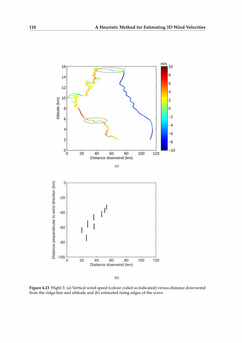
118 A Heuristic Method for Estimating 3D Wind Velocities
0 20 40 60 80 100 1200
2
4
6
8
10
12
14
16
Distance downwind (km)
Alti
tude
(km
)
−10
−8
−6
−4
−2
0
2
4
6
8
10m/s
(a)
0 20 40 60 80 100 120-100
-80
-60
-40
-20
0
Distance downwind (km)
Dis
tan
ce
pe
rpe
nd
icu
lar
to w
ind
dire
ctio
n (
km
)
-10
-5
0
5
10
(b)
Figure 4.23 Flight 3: (a) Vertical wind speed (colour coded as indicated) versus distance downwindfrom the ridge-line and altitude and (b) estimated rising edges of the wave.

4.3 Results 119
20 25 30 35 40 45 50−3
−2
−1
0
1
2
3
4
5
6
Distance downwind from ridge line (km)
Ver
tical
win
d sp
eed
(m/s
)
(a)
30 40 50 60 70 80 90 100−6
−4
−2
0
2
4
6
Distance downwind from ridge line (km)
Ver
tical
win
d sp
eed
(m/s
)
(b)
Figure 4.24 Flight 3: Derived vertical wind speed versus distance downwind from the ridge lineand fitted sinusoids for two flight segments as described in the text for an altitude range of (a)5.3-6.1 km and (b) 15.0-15.6 km.

120 A Heuristic Method for Estimating 3D Wind Velocities
0.2 0.3 0.4 0.5 0.6 0.7 0.8 0.9 10
2
4
6
8
10
12
14
16
Scorer (km−1)
Alti
tude
(km
)
Figure 4.25 Flight 3: The Scorer parameter versus altitude.
ence of trapped stratospheric waves. A calculation of the minimum lee wave wavelengthfrom the Scorer parameter gives approximately 17 km in the troposphere which is sig-nificantly larger than that observed as described above; however the Scorer parameter isincreasing with altitude at 6 km altitude. The minimum wavelength is calculated as 10 kmin the stratosphere. The observed wavelength is larger than this but there is likely to besignificant vertical propagation of the stratosphere wave giving a horizontal wavelengthlarger than the minimum.
The data for this flight also included the heading measured by an electronic compass. Un-fortunately, the type of compass used is unknown. Since a compass is subject to variouserrors, the reliability of the data was considered uncertain enough not to be used for windvelocity estimation. However, once the wind velocity has been determined, the sailplaneheading can be calculated and compared with the measured heading. The calculated andmeasured headings are shown in Fig. 4.26 for two short flight segments. The agreement isquite good. A magnetic compass may be subject to errors when the aircraft is accelerating,particularly when entering and exiting turns, and this is apparent in the figures.
In summary, application of the methods to this flight gave consistent results. The esti-mated horizontal wind velocities are more variable and the speed is somewhat differentfrom the Reanalysis, although the direction agrees quite well. A wave segment seen in thestratosphere may be informative in terms of stratospheric waves.

4.3 Results 121
8500 8550 8600 8650 8700−180
−90
0
90
180
Time (min)
Hea
ding
(°)
7940 7960 7980 8000 8020 8040 8060 8080 8100−180
−90
0
90
180
Time (min)
Hea
ding
(°)
Figure 4.26 Flight 3: Measured heading (solid line) and calculated heading (dashed line) for twoflight segments.

122 A Heuristic Method for Estimating 3D Wind Velocities
230 240 250 260 270 280 2900
1
2
3
4
5
6
7
8
Temperature (K)
Alti
tude
(km
)
Figure 4.27 Flight 4: Temperature versus altitude measured along the ascending flight path (solidline) and descending flight path (dashed line), and the Reanalysis temperature (dot-dashed line).
4.3.4 Flight 4: Perlan Flight 24: Omarama
Flight 4 was flown from Omarama, New Zealand, in the lee of the Southern Alps as de-scribed in Section 3.5. The algorithm was applied to the data using the same parameters asin Table 4.1. The temperature data measured during the flight are collected in 200 m thickaltitude bins, averaged and plotted versus altitude for the ascending and descending por-tions of the flight in Fig. 4.27. The temperature from the Global Reanalysis is shown on thesame graph. The two temperatures agree quite well giving a lapse rate of approximately-5.9 K/km, and the measured temperature data are used for calculations below. The flightwas partitioned into 171 regions, and 51 wind velocity estimates were obtained. Typicalvalues obtained for σw were in the range 0.5-8.9 m/s, and typical values for D were inthe range 3-32. Some of the values of σw were quite large, indicating that the parametersused may not be suitable. Then rregion was reduced to 1000 m and Dmin was increased to5, the flight was partitioned into 273 regions, and 45 estimates were obtained. This gavebetter values of σw in the range 0.4-4.8 m/s, and typical values for D were in the range5.1-30. Some of the σw values are still a bit large however, and are shown versus flight timein Fig. 4.28. Most of the large σw values were on the tow where large variations in windvelocity can be experienced in the rotor at low levels. The other large values are at a timeof approximately 120 mins. The four wind velocities estimates for which σw > 4 m/s wereexcluded from subsequent analysis. The estimated wind velocity is shown in vector formalong the flight path above 3 km in Fig. 4.29(a). The estimated horizontal wind directionis WSW as anticipated from the geopotential plot (Fig. 3.15). Close-ups of two flight seg-ments are shown in Fig. 4.29(b) and (c). The first is near the Northern end of the flight at analtitude of approximately 3.5 km and with flight path parallel to the ridge line. The secondis near the Southern end of the flight at an altitude of approximately 7.0 km and shows

4.3 Results 123
0 50 100 150 200 250 3000
0.5
1
1.5
2
2.5
3
3.5
4
4.5
5
time (min)
σ w (
m/s
)
Figure 4.28 Flight 4: Values of σw versus time.
some short downwind segments. The two flight segments are in separate wave regions, asshown in the topography plot in Fig. 3.14(a). As seen previously, there are fewer estimatesin the first region than the second region, since the first flight path is relatively straight andthe heading changes slowly.
The wind speed and direction estimates were collected into altitude bins 200 m thick andaveraged, separately for the ascending and descending paths of the flight, and are shownabove 2 km in Fig. 4.30. Note that there is a difference in wind direction of up to about40◦ at lower altitudes for the ascending and descending portions of the flight. There couldbe a wind shift between the different locations and times of these flight segments. TheReanalysis wind speed and direction are also shown Fig. 4.30. The estimated wind speedand direction agree quite well with the Reanalysis. The estimated wind speeds are self-consistent so are taken as reliable.
A satellite picture of the southern South Island of New Zealand at 0000Z on 11 August2002 is shown in Fig. 3.17. Although the projection is distorted, wave clouds are evident inthe flight region with a spacing of about 8 km.
Using the fitted temperature profile and the calculated horizontal wind speed, the Scorerparameter is calculated and shown in Fig. 4.31. The Scorer parameter decreases with alti-tude, supporting the development of trapped lee waves. The Scorer parameter varies be-tween 0.3 and 0.6 km−1, with a corresponding minimum lee wave wavelengths between10 and 20 km.
There are no long downwind paths during this flight, but long flight segments parallel

124 A Heuristic Method for Estimating 3D Wind Velocities
−60 −40 −20 0 20 40 60−40
−20
0
20
40
60
80
100
120
Position East (km)
Pos
ition
Nor
th (
km)
(a)
-10 0 10 20 3010
20
30
40
50
60
70
80
90
100
Position East (km)
Po
sitio
n N
ort
h (
km
)
(b)
-42 -40 -38 -36 -34 -32 -30 -28-26
-24
-22
-20
-18
-16
-14
-12
-10
Position East (km)
Po
sitio
n N
ort
h (
km
)
(c)
Figure 4.29 Flight 4: (a) Estimated wind velocity vectors along the flight path. The launch po-sition is shown by the x and the flight path is approximately anticlockwise. (b)(c) wind velocityestimates for two flight segments as described in the text for an altitude range of 3.2-8.1 km and6.7-8.6 km, respectively. The length and direction of the arrows represent the estimated wind speedand direction, respectively.

4.3 Results 125
15 20 25 30 35 400
1
2
3
4
5
6
7
8
9
Wind speed (m/s)
Alti
tude
(km
)
(a)
230 240 250 260 270 280 290 3000
1
2
3
4
5
6
7
8
9
Wind direction (degree)
Alti
tude
(km
)
(b)
Figure 4.30 Flight 4: (a) Horizontal wind speed and (b) direction estimates versus altitude. Theascending portion of the flight is shown by the solid line, and descending portion by the dashedline. The Reanalysis values at Omarama are shown by the dot-dashed line.

126 A Heuristic Method for Estimating 3D Wind Velocities
0.3 0.35 0.4 0.45 0.5 0.55 0.6 0.65 0.70
1
2
3
4
5
6
7
8
9
Alti
tude
(km
)
Scorer (km−2)
Figure 4.31 Flight 4: The Scorer parameter versus altitude for the ascending (solid line) and de-scending (dashed line) flight path.
to the ridge line. An 80-minute flight segment approximately parallel to the long ridgeline at the Northern end of the flight is shown in Fig. 4.32(a). The sailplane is in the samewave system produced by the long ridge line as shown. The flight altitude versus positionNorth is shown in Fig. 4.32(b). The flight path is replotted in Fig. 4.32(c) as a function ofdistance downwind from the ridge line, and colour-coded by the derived vertical windspeed. In Fig. 4.32(c) there are four strong vertical wind speed peaks at positions betweenapproximately 8 and 12 km down wind from the ridge line, indicating the leading edgesof the wave. The altitude varies between 5 and 8 km. Between the leading edges there areweak vertical wind speeds which indicate wave patterns.
In summary, consistent results were obtained for the horizontal wind velocities which arealso consistent with the Reanalysis. The flight consists of long segments parallel to theridge line. Inspection of the estimated vertical wind speeds showed expected patterns rel-ative to the topography. The decreasing Scorer parameter with altitude indicates suitableconditions for production of trapped lee waves.

4.3 Results 127
-10 0 10 20 3020
30
40
50
60
70
80
90
100
110
Position East (km)
Po
sitio
n N
ort
h (
km
)
(a)
4 6 8 1020
30
40
50
60
70
80
90
100
110
Altitude (km)
(b)
0 10 2020
30
40
50
60
70
80
90
100
110
Distance downwind (km)
-1
0
1
2
3
4
5m/s
(c)
Figure 4.32 Flight 4: A flight section parallel to the ridge line as described in the text. (a) Flightpath (thin line) and ridge line (thick line). (b) Flight altitude versus position North. (c) Estimatedvertical wind speed (colour coded as indicated) versus distance downwind from the ridge line.

128

Chapter 5
Flight Simulation
In Chapters 6 and 7, statistical estimation techniques are used to determine wind velocitiesfrom flight data. In order to study the performance of these methods they are applied tosynthetic data from simulated flights. The nature of these simulations is described in thischapter. It is emphasized that the objective is not a full flight simulation, but a specificationof simple flight trajectories in the air in a specified variable wind velocity field of relevanceto mountain wave, and calculation of the resulting noisy flight data.
There are three inputs to the simulator, in addition to the time-step δt:
1. The 3D wind field.
2. The indicated airspeed and heading of the sailplane as a function of time.
3. Sink rate characteristics of the sailplane, i.e. the flight polar.
These inputs are described in turn below.
1. Wind field
The wind field is fixed in time but varies in space. The horizontal component of thewind velocity is defined in terms of its speed and direction, denoted vw(x, y, z) andθw(x, y, z), respectively. The horizontal wind field is defined by the values vw0 =
vw(0, 0, 0) and θw0 = θw(0, 0, 0) at the origin, by linear rates of change of vw(x, y, z)and θw(x, y, z) with x with values A and B, respectively, and a linear rate of changeC, of vw(x, y, z) with z. The horizontal wind field is therefore given by
vw(x, y, z) = vw0 +Ax+ Cz (5.1)
θw(x, y, z) = θw0 +Bx (5.2)
129

130 Flight Simulation
Note that the horizontal wind speed is independent of y and the horizontal wind di-rection is independent of y and z. The vertical wind speed is taken to be a sinusoidalwave generated by a source along the y-axis and takes the form
vzw(x, y, z) = D sin(2πx/λ+ ϕ) (5.3)
where D, λ and ϕ are the maximum vertical wind speed, wavelength and phase shift,respectively. Note that the vertical wind speed is independent of y (as expected fora source on the y-axis) and of z. Although the above definition describes a fairly re-stricted wind field, it is sufficiently general to generate the data required and doesnot introduce any hidden constrains into the inversion.
2. Sailplane airspeed and heading
The sailplane trajectory relative to the air is defined by specifying the indicated air-speed (assumed horizontal) and heading as a function of time, vinda (t) and θa(t), re-spectively. The simulation time-step is δt and the airspeed and heading are thereforediscretized as vinda,i = vinda (iδt) and θa,i = θa(iδt). The simulation is kinematic exceptfor a component of the sailplane vertical speed due to energy exchange that is calcu-lated from the change in airspeed at each time-step. A standard atmosphere model(Section 1.1.1) is used to transform between IAS and TAS. The initial sailplane posi-tion is taken as (0, 0, z0).
3. Sink rate characteristics
The sailplane sink rate is specified as a function of IAS using a given flight polar. Forthe simulations in this thesis the DG505M flight polar at a wing loading of 44 kg/m2
(see Section 3.2) is used.
The output consists of the following parameters as a function of time-step i. Gaussian noiseis added to ground position and airspeed to give data for use in an inversion.
1. Ground position, (xi, yi, zi)
2. Air horizontal position, (xa,i, ya,i)
3. Horizontal ground velocity, (vxg,i, vyg,i)
4. 3D wind velocity, (vxw,i, vyw,i, v
zw,i)
5. TAS, va,i

131
6. Sink rate, vertical speed component due to energy exchange, and vertical groundspeed, (si, ve,i, vzg,i)
7. Rate of change of heading, δθa,i/δt
8. Bank angle, ϕi
9. Noisy ground position data, (xi, yi, zi)
10. Noisy ground velocity data, (vxg,i, vyg,i, v
zg,i)
11. Noisy IAS and heading data, (vinda,i , θa,i)
The flight path and related quantities are calculated by linear prediction with a time-step ofδt. Since all quantities are slowly varying, this is sufficiently accurate for sufficiently smallδt. Given all quantities at time-step i, values at time-step i + 1 are updated as follows. Aflow diagram of the simulator is shown in Fig. 5.1. The new air position is first calculatedas
xa,i+1 = xa,i + va,i cos(θa,i)δt,
ya,i+1 = ya,i + va,i sin(θa,i)δt. (5.4)
The horizontal ground velocity is calculated as
vxg,i = vxw,i + vxa,i,
vyg,i = vyw,i + vya,i, (5.5)
and the ground position is updated as
xi+1 = xg,i + vxg,iδt,
yi+1 = yg,i + vyg,iδt. (5.6)
The TAS va,i is calculated from vinda,i and zi, the vertical ground speed is calculated using
si = −(va,i/vinda,i )s0(v
inda,i )
ve,i = −(va,i/g)(va,i − va,i−1)/δt
vzg,i = vzw,i + si + ve,i, (5.7)
and the vertical ground position then updated as
zi+1 = zi + vzg,iδt. (5.8)
To illustrate use of the simulator, an example of the input and output for a simulation isshown in Figs. 5.2 and 5.3. Parameters used in the simulation are δt = 0.1 s, Nt = 1000 s,

132 Flight Simulation
Input: vinda,i , θa,i ,
z0, δt, and N t
Initialize: i = 1,
x1 = y1 = 0, z1 = z0
Input: vw0, θw0, A,
B, C, D, λ and φ
Calculate horizon-
tal wind velocity
(vxw ,i , v
yw ,i ) at ground
position (x i , yi , zi )
Calculate vertical wind
speedvzw ,i at ground
position(x i , yi , zi )
Calculate TAS
va,i at time step i
Calculate horizontal air
position (xa,i +1 , ya,i +1 )
at time step i + 1i = i + 1
Calculate horizon-
tal ground velocity
(vxg,i , v
yg,i ) at time step i
Calculate horizon-
tal ground posi-
tion (x i +1 , yi +1 )
at time step i + 1
Calculate si from vinda,i
Calculate ve,i from vinda,i
and vinda,i +1
Calculate vzw ,i +1 from si ,
ve,i , and vw ,i
Calculate zi +1 at
time step i + 1
Figure 5.1 Flow diagram of the flight simulator.

133
z0 = 3 km, vw0 = 35 m/s, θw0 = 305◦, A = −0.5 m/s/ km, B = 1◦/ km, C = 1 m/s/ km,D = 3 m/s, λ = 10 km, and ϕ = π/6. Noise was not added to the output data.
The resulting wind field is shown in Fig. 5.3(a) and (b). The airspeed used is a 1000 ssegment taken from Flight 1 (Section 3.2), linearly interpolated onto a sampling intervalof 1 s, and shown in Fig. 5.2(c). The heading function used is shown in Fig. 5.2(d) andincorporates a number of turns and straight flight segments. The resulting air path andground path are shown in Fig. 5.3.
To check that δt = 0.1 s is small enough, the simulation was repeated with δt = 0.02 s, andthe outputs from the two simulations compared. The average differences in position andground velocity data are 1.3 m and 0.02 m/s respectively. The differences in position andvelocity are both very small. This shows that δt = 0.1 s gives sufficient accuracy for theprecision required, i.e. the errors are smaller than typical levels of noise added to the data.

134 Flight Simulation
−10 −5 0 5 10 15 20−30
−25
−20
−15
−10
−5
0
x (km)
y (k
m)
(a)
−10 −5 0 5 10 15 20−3
−2
−1
0
1
2
3
x (km)
v wz (
m/s
)
(b)
0 200 400 600 800 100022
24
26
28
30
32
34
t (s)
v aind (
m/s
)
(c)
0 200 400 600 800 1000−200
−150
−100
−50
0
50
100
150
200
t (s)
θ a (°)
(d)
Figure 5.2 Input data for the simulation generated for δt = 0.1 s showing (a) horizontal wind speed,(b) vertical wind speed, (c) indicated airspeed, and (d) heading.

135
−5 0 5 10 15 20−30
−25
−20
−15
−10
−5
0
x (km)
y (k
m)
(a)
0 200 400 600 800 10002.5
2.6
2.7
2.8
2.9
3
3.1
3.2
3.3
t (s)
z (k
m)
(b)
−10 −8 −6 −4 −2 0 2 4−8
−6
−4
−2
0
2
xa (km)
y a (km
)
(c)
Figure 5.3 Output data from the simulation generated for δt = 0.1 s showing (a) ground path, (b)altitude, and (c) air path.

136

Chapter 6
Maximum Likelihood Estimation
6.1 Introduction
The heuristic method described in Chapter 4 provides good solutions to the problem ofwind velocity estimation where GPS and airspeed data are available. The method is spe-cific however to ground velocity and airspeed data. It could be extended to other kindsof data (e.g. heading data) but this would require a reformulation. It is therefore not aparticularly general formulation of the problem. Furthermore, the method does not in-corporate a rigorous noise model. The cylindrical regions are large and hence the windvelocity estimates obtained are quite sparse. When the noise level increases the reliabilityof the heuristic method reduces, and better data and noise models are required.
In this chapter and Chapter 7, the problem of wind velocity estimation is formulated asa general statistical estimation problem. This is a standard formulation that allows incor-poration of, in principle, any data and any constraints or a priori information, and allowsincorporation of explicit noise models and the application of standard estimation meth-ods. In this chapter, maximum likelihood (ML) estimators are developed for wind velocityestimation from data consisting of ground velocity and either airspeed or heading data.The methods are illustrated by application to simulated and real flight data. In Chapter 7,the problem of wind velocity estimation from only ground velocity data is addressed, andmaximum a posteriori (MAP) estimators are developed, and also applied to simulated andexperimental data.
As described in Chapter 2, the 3D problem can be decomposed into the horizontal andvertical components. This decomposition is continued here. As seen in Chapters 2 and4, the 2D problem of determining the horizontal component of the wind velocity is themore difficult problem, the vertical problem being relatively straightforward. Therefore, inthis chapter, only the 2D problem is considered, i.e. determination of the horizontal windvelocity from a flight at constant altitude. This is sufficient to illustrate the ML estimator.In Chapter 7, the focus is still on the horizontal component of the wind velocity, but the
137

138 Maximum Likelihood Estimation
3D problem is considered where the horizontal component of the wind velocity varies inthree dimensions. Calculation of the vertical wind speed, using the estimated horizontalcomponent, is also considered there.
In the context of statistical estimation it is convenient to make a small change to some ofthe symbols used in the previous chapters to represent the flight variables. This is becauseit is conventional in the statistical estimation literature to use a vector to represent a col-lection of values of a parameter of interest (refer to Section 1.4). For example, the vectorx = (x1, x2, ...xN ) may be used to represent an image, where the components xi repre-sent the values (brightness) of the N pixels of the image. Following this convention, forexample, the vector vg is used to represent a collection of ground velocities at differenttime instants, i.e. vg = {vg,i}, where the vg,i are the ground velocities at time-point i. Ifit is necessary to refer to the components of vg,i, then the symbols vxg,i and vyg,i are used.Furthermore, the vectors vg, vg, and vg are used to represent the true, measured, and es-timated ground velocities, respectively, and the same for other quantities. Similarly, thevectors vw, va, θa are used to represent a collection of of wind velocities, airspeeds andheadings, respectively. Note that va does not represent a collection of air velocities, andthis particular collection of quantities is not used.
6.2 Measurement model
Referring to Section 1.4, the measurement model describes the measurement (data), includ-ing noise, in terms of the object parameters. In the case at hand, the measurement model isquite simple. The data are the ground velocities and airspeed and/or heading. The objectparameters are the true ground, wind and air velocities. However, since these are not allindependent, the ground and wind velocities are used as the object parameters.
The measured ground velocities are related to the true ground velocity components by
vg,i = vg,i + ng,i, (6.1)
where ng,i represents the measurement noise. Errors in GPS positioning have been inves-tigated in [80] for consumer-grade GPS receivers with standard positioning service, non-differential GPS. Measurements show that the distribution of horizontal GPS fixes can beapproximated by an uncorrelated, bivariate normal distribution, i.e. the (Northerly andEasterly) components are normally distributed. They also show that the position errorsare quite strongly correlated (correlation coefficient > 0.6) for fixes less than one minuteapart. As a result, calculation of the horizontal velocity from differences in GPS fixes lessthan one minute apart will cancel out these errors to some degree. They also show that thevertical fixes show approximately Gaussian errors, with a standard deviation of about 5 m,sometimes with a significant bias which may be up to 10 m. The bias is due primarily tovariations in ionospheric delay. The effects of the ionosphere generally change slowly intime so that the bias changes slowly with time. Therefore, the bias errors will tend to cancel
6.2 Measurement model 139
out when calculating the vertical velocity. An appropriate model for each component ofthe error ng,i is therefore zero-mean, white Gaussian noise. The variance, denoted σ2
g , canthen be estimated from known GPS characteristics.
The airspeed data are assumed to have been corrected, if necessary, for air density usingstandard methods to give the true airspeed. As described in Chapter 2, the airspeed andits horizontal component are assumed to be equal. The measured airspeed at time-step i isthen given by
va,i = ||vg,i − vw,i||+ na,i, (6.2)
where na,i represents the airspeed indicator errors. The primary errors in a pitot-static air-speed indicator are additive pneumatic disturbances [52] and the disturbance in the impact(dynamic) pressure can be approximated as Gaussian. Since the airspeed is proportionalto the square-root of the impact pressure, the errors in the derived airspeed will not bestrictly Gaussian. However, for convenience we assume that the noise na,i can be modeledapproximately by zero-mean, white Gaussian noise since the errors are small compared tothe airspeed. The variance, denoted σ2
a, can be obtained from the instrument specifications.
The aircraft heading measurements are given by
θa,i = tan−1(vg,i − vw,i) + nθa,i, (6.3)
where nθa,i are the compass errors, modeled as zero-mean, white Gaussian noise with vari-ance σ2
θa, and tan−1(x) is the four-quadrant inverse tangent that gives an angle on (−π, π)
for the vector argument x. The variance σ2θa
is considered to be small enough that wrap-ping of the distribution on (−π, π) is not a problem. Equations (6.1), (6.2) and (6.3) togetherform the measurement model.
In the next three sections, three different kinds of data sets are considered, consisting ofground velocity, airspeed and heading; ground velocity and airspeed; and ground veloc-ity and heading, respectively. ML estimators are developed for each case and tested onsimulated and experimental data.

140 Maximum Likelihood Estimation
6.3 Position, airspeed and heading data
6.3.1 Methods
Consider data consisting of ground velocity, airspeed and heading. The velocity relative tothe air is given by the airspeed and heading so that, the wind velocity at each time-step isgiven simply by
vw,i = vg,i − va,i. (6.4)
However, at a single time-step, the number of parameters is equal to the number of data,so that such an estimate would be sensitive to noise. The sensitivity can be reduced byexploiting the assumption of a constant (or slowly varying) wind velocity field, using datafrom a number of contiguous time-steps, and taking a statistical estimation approach.
Consider a temporal window (i−N, i+N) centered at time-step i and with half width N . Ifthe wind velocity is assumed to be constant within this window then the object parametersare
(vg,i, vw,i) = (vg,i−N , ..., vg,i+N , vw,i) , (6.5)
and the data are
(vg,i, va,i, θa,i) =(vg,i−N , va,i−N , θa,i−N , ..., vg,i+N , va,i+N , θa,i+N
). (6.6)
The data-to-parameter ratio is now 4(2N + 1)/[2(2N + 1) + 2] ≈ 2, and the problem isover-determined. Using the assumption of Gaussian noise, the likelihood function is
p(vg,i, va,i, θa,i|vg,i, vw,i
)= K1
N∏j=−N
exp(− ||vg,i+j − vg,i+j ||2/2σ2
g
− (va,i+j − ||vg,i+j − vw,i||)2 /2σ2a −
(θa,i+j − tan−1(vg,i+j − vw,i)
)2/2σ2
θa
),
(6.7)
where K1 is a constant. Care must be taken when calculating the differences in the lastterm to account for wrapping on (−π, π). The maximum likelihood estimate of the objectparameters is then given by
(vg,i, vw,i)ML = argmax(vg,i,vw,i)
{p(vg,i, va,i, θa,i|vg,i, vw,i
)}. (6.8)
The minimisation begins with starting values for (vg,1, vw,1), and the estimated values(vg,i, vg,i) are used as the starting values for solving for (vg,i+1, vw,i+1). The maximisa-
tion in (6.8) was performed by minimising − ln(p(vg,i, va,i, θa,i|vg,i, vw,i
)) using the Mat-
lab function fminunc [81]. The function fminunc employs a local minimiser using theBFGS Quasi-Newton method with a cubic line search procedure [82, 83]. The terminationcriterion is based on specified values of the maximum number of function evaluations,maximum number of iterations and tolerance of the optimised variable or the cost func-

6.3 Position, airspeed and heading data 141
tion. Suitable termination criteria were selected by experimentation.
6.3.2 Simulation results
The performance of the ML estimator is illustrated using simulated flight data generatedas described in Chapter 5. Two flights with different headings were used. The parametersused in the simulation were δt = 0.02 s, Nt = 1000 s, vw0 = 35 m/s, θw0 = 305◦, A = −1
m/s/km, B = 2◦/km, C = 0, and D = 0. This gives the wind field as shown in Fig. 6.1(a),and the wind direction is approximately northwest. The airspeed data were taken froma segment of Flight 1 (Section 3.2) and linearly interpolated onto a sample spacing of δtas shown in Fig. 6.1(b). The headings for the two flights are shown in Fig. 6.2(a) and (b)respectively, and the paths relative to the air in (c) and (d). During the first flight thesailplane performs a number of circling maneuvers at turn rates of 1 − 3◦/s. The secondflight is relatively straight with a few high rate turns at 5◦/s and 20◦/s. The ground pathsfor the two flights are shown in Fig. 6.2(e) and (f) respectively. Measurements of the groundvelocity, airspeed, and heading were taken at 1 s intervals and corrupted by noise withstandard deviations of 2 m/s, 2 m/s, and 2◦, respectively.
The ML estimates were calculated as described above using N = 20 with known valuesof σg, σa, and σθa . A starting value of (25 m/s, 315◦) was used in the optimisation com-pared to the true value of (35 m/s, 305◦). The estimated wind speed and direction fromFlight 1 are shown in Fig. 6.3(a) and (b) respectively, and the true values are shown forcomparison. Note that the wind speed and direction estimates were not obtained at everysingle time step, but one in each window. The average rms errors across the whole flightare 0.24 m/s and 0.66◦. The estimates correctly track the true wind velocity. For compar-ison, the estimates calculated directly from (6.4) are shown in Fig. 6.3 (c) (d), which givesan average rms error of 1.8 m/s and 4.2◦. However, averaging these results over a windowof halfwidth 20 s reduces the error to 0.22 m/s and 0.65◦, as shown in Fig. 6.3(e)(f).
For Flight 2, the ML results are shown in Fig. 6.4 (a)(b). The average rms errors in the MLestimates are 0.29 m/s and 0.55◦, those for the direct calculation are 2.0 m/s and 3.9◦ in(c)(d), and averaging gives 0.31 m/s and 0.52◦ as shown in (e)(f). The performance of theML estimates for the complete data is more-or-less the same as values calculated directlyand averaged over the temporal window. A more significant advantage of the statisticalestimation accrues when the data are incomplete as described in the following subsections.

142 Maximum Likelihood Estimation
0 5 10 15 20-20
-15
-10
-5
0
xg
(km)
yg
(km
)
(a)
0 200 400 600 800 100022
24
26
28
30
32
34
t (s)
v a (m
/s)
(b)
Figure 6.1 (a) Vector wind field and (b) airspeed for the simulated flights.

6.3 Position, airspeed and heading data 143
0 200 400 600 800 1000−200
−150
−100
−50
0
50
100
150
200
t (s)
head
ing
(°)
(a)
0 200 400 600 800 1000−200
−150
−100
−50
0
50
100
150
200
t (s)
head
ing
(°)
(b)
-5 -4 -3 -2 -1 0 1-1
0
1
2
3
4
5
6
xa
(km)
ya
(km
)
(c)
-10 -8 -6 -4 -2 0 2 4-6
-4
-2
0
2
4
6
xa
(km)
ya
(km
)
(d)
0 5 10 15 20-20
-15
-10
-5
0
xg
(km)
yg
(km
)
(e)
-5 0 5 10 15 20-25
-20
-15
-10
-5
0
xg
(km)
yg
(km
)
(f)
Figure 6.2 Heading versus time of Simulated Flight 1 (a) and 2 (b), flight path relative to the air offlight 1 (c) and 2 (d), and flight path relative to the ground of flight 1 (e) and 2 (f).

144 Maximum Likelihood Estimation
0 200 400 600 800 100015
25
35
45
t (s)
vw
(m/s
)
(a)
0 200 400 600 800 1000270
290
310
330
350
t (s)
θw
(°)
(b)
0 200 400 600 800 100015
25
35
45
t (s)
vw
(m/s
)
(c)
0 200 400 600 800 1000270
290
310
330
350
t (s)
θw
(°)
(d)
0 200 400 600 800 100015
25
35
45
t (s)
vw
(m/s
)
(e)
0 200 400 600 800 1000270
290
310
330
350
t (s)
θw
(°)
(f)
Figure 6.3 Simulated Flight 1: (a) Wind speed and (b) direction estimated from the ground velocity,airspeed and heading data (crosses), and (c) wind speed and (d) direction calculated directly fromthe data (crosses), and (e) wind speed and (f) wind direction calculated directly from the data andaveraged over a time window (crosses). The true values are shown by the solid lines.
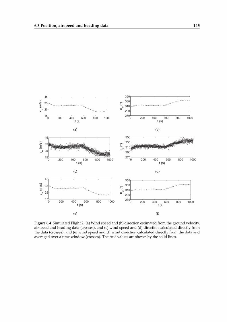
6.3 Position, airspeed and heading data 145
0 200 400 600 800 100015
25
35
45
t (s)
vw
(m/s
)
(a)
0 200 400 600 800 1000270
290
310
330
350
t (s)θ
w(°
)
(b)
0 200 400 600 800 100015
25
35
45
t (s)
vw
(m/s
)
(c)
0 200 400 600 800 1000270
290
310
330
350
t (s)
θw
(°)
(d)
0 200 400 600 800 100015
25
35
45
t (s)
vw
(m/s
)
(e)
0 200 400 600 800 1000270
290
310
330
350
t (s)
θw
(°)
(f)
Figure 6.4 Simulated Flight 2: (a) Wind speed and (b) direction estimated from the ground velocity,airspeed and heading data (crosses), and (c) wind speed and (d) direction calculated directly fromthe data (crosses), and (e) wind speed and (f) wind direction calculated directly from the data andaveraged over a time window (crosses). The true values are shown by the solid lines.

146 Maximum Likelihood Estimation
6.4 Position and airspeed data
6.4.1 Methods
Although sailplanes always have an airspeed indicator and a compass, data from the latterare usually not logged as described previously. In this section, the case of data consisting ofground velocity and airspeed is considered. As described in Chapters 2 and 4, at a singletime step this data provides a one-parameter family of solutions for the wind velocity,although for data at multiple time steps with a constant wind velocity the ambiguity isresolved if the heading of data used for an estimate are sufficiently different. The estimatesare more stable for larger heading differences. As shown in Section 2.2.2, the dependenceon heading difference translates into differences in ground velocity. The data vector in thiscase is denoted
(vg,i, va,i) = (vg,i−N , va,i−N , ..., vg,i+N , va,i+N ) . (6.9)
The data-to-parameter ratio is now 3(2N + 1)/[2(2N + 1) + 2] ≈ 1.5 and the problem isover-determined. Using the assumption of Gaussian noise, the likelihood function is
p (vg,i, va,i|vg,i, vw,i) = K2
∏j
exp(− ||vg,i+j − vg,i+j ||2/2σ2
g
− (va,i+j − ||vg,i+j − vw,i||)2/2σ2a
),
(6.10)
where K2 is a constant. The ML estimate is then
(vg,i, vw,i)a,ML = argmax(vg,i,vw,i)
{p (vg,i, va,i|vg,i, vw,i)} , (6.11)
where the subscript a on the LHS indicates “airspeed data only.”
6.4.2 Simulation results
Using the same two simulated flight in Section 6.3.2 with no heading data, and the datawere corrupted by noise as described. The ML estimates of the wind velocity were calcu-lated as described above using the known values of the noise variances and N = 20 andthe same starting values as in Section 6.3.
The estimated wind speed and direction for Flight 1 are shown in Fig. 6.5(a) and (b) re-spectively. The rms errors in the estimated wind speed and direction are 1.2 m/s and 2.1◦.The estimated values are quite consistent with the true values, as the heading differencesin this flight are sufficiently large for obtaining good estimates.
For Flight 2 the results are shown in Fig. 6.6(a) and (b) respectively. In this case the esti-mates track the true values some of the time but drift off at other times. The rms errors inthe estimated wind speed and direction 6.2 m/s and 38◦. A plot of the rate of change ofheading (Fig. 6.6(c)) shows that the errors occur when the heading is constant or slowly-

6.4 Position and airspeed data 147
0 200 400 600 800 100015
25
35
45
t (s)
vw
(m/s
)
(a)
0 200 400 600 800 1000270
290
310
330
350
t (s)
θw
(°)
(b)
Figure 6.5 Simulated Flight 1: (a) Wind speed and (b) direction (crosses) estimated from the groundvelocity and airspeed data, and the true wind speed and direction (solid lines).
changing as anticipated from Section 2.2.2. Inspection of Fig. 6.6 shows that the estimatesdrift off the true values when the heading is constant, and converge back to the true valuesat t = 100, 300, 500, 700, 800 s when the sailplane turns.
The instability due to an ambiguity at small heading angle differences is illustrated by plot-ting the likelihood functions. Two flight segments from the simulated flight were chosen asshown in Fig. 6.7. Flight segment A is almost straight and has small heading differences,and flight segment B is in a turn has large heading differences. 2-D slices of the multi-dimensional log likelihood functions for the x and y components of the wind velocity atthe correct values of the other parameters are shown in Fig. 6.8. Fig. 6.8(a) and (b) show asuperposition of the individual factors of the likelihood functions for time-steps i − 10, i,and i+ 10, for flight segment A and B, respectively. The corresponding full likelihoods areshown in Fig. 6.8(c) and (d). For large changes in the heading (Fig. 6.8(b) and (d)), the cir-cles corresponding to the individual factors are distinct and the mutual overlap in a singleregion gives a likelihood function that, although multi-modal, has two well-defined globalmaxima. Measurement noise can, in some cases, produce a higher value for the secondarymaximum causing the estimate to drift to the incorrect maximum. The error corrects oncethe heading changes. However for small changes in the heading (Fig. 6.8(a) and (c)), thecircles are similar, giving a broad maximum in the likelihood function.
To investigate the effect of changing the parameter σg, it was increased to 10 m/s withthe other parameters values unchanged, the optimisation repeated for Simulated Flight 2,and the results are shown in Fig. 6.9(a) and (b). The estimates are significantly improvedand rms errors are 2.3 m/s and 6.7◦. In particular, the large errors at the flight sectionswith constant heading are improved significantly. Increasing σg presumably reduces thedependency of the estimates on the ground velocity data, hence when there is an ambiguitydue to a constant heading, the wind velocity estimates are driven more by the startingvalues at time-step i + 1 being the estimated values at time-step i, so the estimates do nottend to drift off as rapidly. Results obtained when increasing σa to 10 m/s are shown in (c)and (d). There is no overall improvement in this case with rms errors of 5.4 m/s and 79◦,suggesting that the airspeed data are more important than the ground velocity data in thiscase. Note that some of the wind direction estimates are so large that they lie outside therange of the figure.

148 Maximum Likelihood Estimation
0 200 400 600 800 100015
25
35
45
t (s)
vw
(m/s
)
(a)
0 200 400 600 800 1000270
290
310
330
350
t (s)
θw
(°)
(b)
0 200 400 600 800 1000−5
0
5
10
15
20
t (s)
dθa (
°/s)
(c)
Figure 6.6 Simulated Flight 2: (a) Wind speed and (b) direction (crosses) estimated from the groundvelocity and airspeed data, and the true wind speed and direction (solid lines). (c) Heading differ-ences versus time.

6.4 Position and airspeed data 149
−10 −8 −6 −4 −2 0 2 4−5
−4
−3
−2
−1
0
1
2
3
4
xa (km)
y a (km
)
B
A
Figure 6.7 Air path showing two flight segments selected with small (A) and large (B) groundcurvatures indicated in circles and crosses respectively.
6.4.3 Experimental results
The ML estimator was applied to the data from Flight 1 (Section 3.2), using the positionand airspeed data and N = 40 s (i.e. time window length 81 s), σg = 2 m/s, σa = 2 m/s,σθa = 2◦ to estimate the wind velocities. The wind speed and direction estimates are shownin Fig. 6.10, and compared with those obtained using the heuristic method (Chapter 4)as shown in Section 4.3.1. There is good agreement between the two methods with rmsdifferences of 2.2 m/s and 6.2◦, showing the utility of the ML approach.

150 Maximum Likelihood Estimation
vwx, m/s
vw y, m
/s
−150 −100 −50 0 50 100 150
−100
−50
0
50
100
(a)
vwx, m/s
vw y, m
/s
−150 −100 −50 0 50 100 150
−100
−50
0
50
100
(b)
vwx, m/s
vw y, m
/s
−100 0 100
−100
−50
0
50
100
(c)
vwx, m/s
vw y, m
/s
−100 0 100
−100
−50
0
50
100
(d)
Figure 6.8 Log-likelihood functions using position and airspeed data only for well and ill-determined solutions. Three factors of the likelihood function are shown in (a) and (b), wherethe gray region represents the mean ±2 m/s standard deviations. The full likelihood is shown in(c) and (d), where the gray level represents the log likelihood. The regions of the path used for theill (a,c) and well-determined (b,d) estimates are the segments A and B shown in Fig. 6.7.

6.4 Position and airspeed data 151
0 200 400 600 800 100015
25
35
45
t (s)
vw
(m/s
)
(a)
0 200 400 600 800 1000270
290
310
330
350
t (s)
θw
(°)
(b)
0 200 400 600 800 100015
25
35
45
t (s)
vw
(m/s
)
(c)
0 200 400 600 800 1000270
290
310
330
350
t (s)
θw
(°)
(d)
Figure 6.9 Simulated Flight 2: Wind speed and direction estimated from the ground velocity andairspeed data (crosses) and the true wind speed and direction (solid lines), (a)(b) using σg = 10 m/s,and (c)(d) using σa = 10 m/s.

152 Maximum Likelihood Estimation
50 100 150 200 250 3000
10
20
30
40
50
60
win
d sp
eed
(m/s
)
time (min)
(a)
50 100 150 200 250 300200
210
220
230
240
250
260
270
280
290
300
win
d di
rect
ion
(°)
time (min)
(b)
Figure 6.10 Wind speed and direction estimated from position and airspeed data for Flight 1 usingthe ML estimator (crosses) and the heuristic method of Chapter 4 (circles).

6.5 Position and heading data 153
6.5 Position and heading data
6.5.1 Method
Consider now the case when airspeed data is not available but the heading is measured, inaddition to the ground velocity. The data vector is now
(vg,i, θa,i) =(vg,i−N , θa,i−N , ..., vg,i+N , θa,i+N
). (6.12)
The data-to-parameter ratio is 1.5 as in the previous case. As described in Chapter 2, for asingle time-step the solution is a one parameter family that lies on a line. For multiple datain a constant wind field, the solution lies on the intersection of two lines, giving a uniquesolution for different headings with no noise. The likelihood function is now
p(vg,i, θa,i|vg,i, vw,i
)=K3
∏j
exp(− ||vg,i+j − vg,i+j ||2/2σ2
g
− [θa,i+j − tan−1(vg,i+j − vw,i)]2/2σ2
θa
),
(6.13)
where K3 is a constant. The ML estimate is then
(vg,i, vw,i)h,ML = argmax(vg,i,vw,i)
{p(vg,i, θa,i|vg,i, vw,i
)}, (6.14)
where the subscript h on the LHS indicates “heading data only.”
6.5.2 Simulation results
For the same two simulated flights described in the previous sections with no airspeeddata, the ML estimates of the wind velocity were calculated as described above using theknown values of the noise variances and N = 20. The results for Flight 1 are shown inFig. 6.11(a) and (b). The estimates closely match the true values and the average rms errorsare 0.50 m/s and 1.6◦.
0 200 400 600 800 100015
25
35
45
t (s)
vw
(m/s
)
(a)
0 200 400 600 800 1000270
290
310
330
350
t (s)
θw
(°)
(b)
Figure 6.11 Simulated Flight 1: (a) Wind speed and (b) direction estimated from ground velocityand heading data (crosses), and the true wind speed and direction (solid lines).

154 Maximum Likelihood Estimation
0 200 400 600 800 100015
25
35
45
t (s)
vw
(m/s
)
(a)
0 200 400 600 800 1000270
290
310
330
350
t (s)
θw
(°)
(b)
Figure 6.12 Simulated Flight 2: (a) Wind speed and (b) direction estimated from ground velocityand heading data (crosses), and the true wind speed and direction (solid lines).
For Flight 2 the results are shown in Fig. 6.12(a) and (b). As with the case for positionand airspeed data, the results are not as good for this flight as a result of the regions withconstant heading. This is evident where the estimates diverge near i = 400. The rmserrors in the estimated wind speed and direction 6.4 m/s and 7.0◦, respectively, which isparticularly large for the airspeed.
Using data from flight segments A and B in Fig. 6.7, the individual likelihood functionsfor i − 10, i, and i + 10 are shown in Fig. 6.13(a) and (b), respectively. The full likelihoodfunctions are shown in Fig. 6.13 (c) and (d). Inspection of the figure shows a single well-defined maximum for the case B of large changes in heading, whereas for small changes inheading (case A) the maximum of the likelihood function occurs on a long, narrow ridge.The presence of noise can shift the peak along this ridge, lending to estimates that driftalong the ridge.
The effect of increasing σg to 10 m/s is shown in Fig. 6.14. The estimates for the flightsegments with constant heading are improved significantly (rms errors of 2.4 m/s and3.8◦), for the same reasons as described in the previous section. The effect of increasing σθato 5◦ is shown in (c) and (d). The results are quite unstable and most of the wind speedestimates are far off the true values (outside the range shown in the figure), showing theimportance of the heading data.
6.5.3 Experimental results
The ML estimator was applied to data from Flight 1 (Section 3.2). The heading data werederived from the wind velocity estimated using the heuristic method, and interpolatedonto the flight time. Gaussian noise with a standard deviation of 2◦ was added to theheadings. The parameters used were N = 40, σg = 2 m/s, and σθa = 2◦. The resultsare shown in Fig. 6.15(a) and (b), and compared with those obtained using the heuristicmethod that uses ground velocities and airspeed data. The results show reasonably goodagreement between the two methods, with rms errors of 2.7 m/s and 5.0◦, given that theheading data as calculated has limited accuracy.

6.5 Position and heading data 155
vwx, m/s
vw y, m
/s
−150 −100 −50 0 50 100 150
−100
−50
0
50
100
(a)
vwx, m/s
vw y, m
/s
−150 −100 −50 0 50 100 150
−100
−50
0
50
100
(b)
vwx, m/s
vw y, m
/s
−100 0 100
−100
−50
0
50
100
(c)
vwx, m/s
vw y, m
/s
−100 0 100
−100
−50
0
50
100
(d)
Figure 6.13 Log-likelihood functions using position and heading only for well and ill-determinedsolutions. Three factors of the likelihood function are shown in (a) and (b), where the gray regionrepresents the mean ±2◦ standard deviations. The full likelihood is shown in (c) and (d), wherethe gray level represents the log likelihood. The regions of the path used for the well-(a,c) andill-determined (b,d) estimates are shown in Fig. 6.7.

156 Maximum Likelihood Estimation
0 200 400 600 800 100015
25
35
45
t (s)
vw
(m/s
)
(a)
0 200 400 600 800 1000270
290
310
330
350
t (s)
θw
(°)
(b)
0 200 400 600 800 100015
25
35
45
t (s)
vw
(m/s
)
(c)
0 200 400 600 800 1000270
290
310
330
350
t (s)θ
w(°
)
(d)
Figure 6.14 Simulated Flight 2: Wind speed and direction estimated from the ground velocity andheading data (crosses) and the true wind speed and direction (solid lines), (a)(b) using σg = 10 m/s,and (c)(d) using σθa = 5◦.
6.6 Discussion
In summary, ML estimation provides a more formally-based method for estimating thewind velocities than that described in Chapter 4. It allows incorporation of different kindsof data as well as noise models. The results show that ML estimation is effective when theproblem is overdetermined.

6.6 Discussion 157
0 50 100 150 200 250 3000
5
10
15
20
25
30
35
40
45
win
d sp
eed
(m/s
)
time (min)
(a)
0 50 100 150 200 250 300200
220
240
260
280
300
320
340
win
d di
rect
ion
(°)
time (min)
(b)
Figure 6.15 (a) Wind Speed and (b) direction estimates calculated from ground velocity and derivedheading data (derived as discussed in the text) for Flight 1 using the ML estimator (crosses), andthose obtained using the heuristic method (circles) as described in Chapter 4.

158

Chapter 7
Maximum a posteriori Estimation
7.1 Introduction
As described previously, the instrumentation installed in most sailplanes records only theGPS position during a flight so that only the ground velocity is measured. Therefore, amethod to estimate wind velocities from this data would be applicable to a wider varietyof flights than would the methods described previously that use airspeed or heading. Thisis the problem addressed in this chapter. The problem is highly underdetermined andthe approach taken is to solve the problem by using a variety of prior information andMaximum a posteriori (MAP) estimation. The methods are applied to simulated and actualflight data.
Determination of the wind velocity in this case is highly underdetermined and, as de-scribed in Section 2.2.4 there is a two-parameter family of solutions. However, in the caseof a sailplane flying in mountain wave there is considerable a priori information that canbe used to constrain the solution. As described previously, the wind field in high-altitudemountain wave varies slowly over the flight path. Furthermore, there are also constraintson the sailplane air velocity. The range of possible values of the airspeed is limited and atypical distribution of airspeeds can be estimated. Also the turn rate (the rate of change ofheading) of the sailplane has an upper bound and also a typical distribution. MAP estima-tors for the wind velocity are developed here using ground velocity data and these kindsof prior information.
The sailplane flight logger records GPS position at regular intervals and these are used tocalculate the ground velocity at each time-step by central differences as described previ-ously. Two kinds of prior information are considered, one concerning the sailplane flightdynamics and the other concerning the wind field.
The velocity of the sailplane through the air can be parameterised by its airspeed and head-ing. Neither of these parameters are completely unconstrained. The airspeed must be be-
159

160 Maximum a posteriori Estimation
tween the stall speed and the maximum allowable speed of the aircraft, and these speedswill be known for a particular sailplane. Furthermore, in a wave flight much of the flightwill be flown at, or close to, the minimum sink airspeed (while climbing), and much ofthe remainder of the flight will be flown close to the maximum maneuvering airspeed (be-tween climbs). These speeds will also be known. Therefore, it is possible, at least in prin-ciple, to build up a reasonably faithful prior density for the airspeed, based on previousflight behavior. Such prior densities are described in Section 7.2.
There is a maximum rate at which a sailplane turns during normal flight. Typically, amaximum turn rate would be about one turn in 10 seconds so that the maximum rateof change of heading is limited to about 40◦/sec. This is an extreme case however, andcorresponds to a steep (or high-bank or tight) turn. Although sailplane pilots perform steepturns, and they may be common in thermal flights, they are infrequent once a sailplane isestablished in a wave system. During a wave flight, the turn rate is very low during muchof the flight while the sailplane is climbing, and is larger while the pilot is maneuveringbetween climbs. Overall, the average rate of change of heading during a wave flight will bevery small. Appropriate prior distributions for the rate of change of heading are describedin Section 7.3.
The methods described in previous chapters are based on an assumption of a constantwind velocity within an appropriate temporal or spatial region. An important advantage ofthe Bayesian approach is that more flexible constraints can be applied to the wind velocity.For fixed meteorological conditions, an atmospheric mountain wave structure (the spatialdistribution of wind velocities) is fixed relative to the terrain. In high-altitude mountainwaves (above the effects of the terrain or about 5000 m altitude), the wind velocity variesslowly with horizontal position (the variation with altitude can be more rapid - see below).For example, we would expect the horizontal component of the wind velocity to vary by nomore than about 10% over distances of the order of 10 km. Furthermore, the meteorologicalconditions tend to vary slowly with time, and the overall wind field structure is often fairlystable over periods of about 30 minutes. Typical wind speeds in mountain waves are 10 -50 m/s and typical sailplane airspeeds 25 - 50 m/s, so that ground speeds vary between0 and 100 m/s. On average then, the sailplane would cover approximately 100 km in 30minutes. Therefore, temporal changes in the wind velocity experienced by sailplane tendto be dominated by the effect of its changes in position rather than by the temporal changein the wind field itself.
The variation of horizontal wind velocity with altitude is usually more rapid than its vari-ation with horizontal position. In fact, as seen in Section 1.2, the development of lee wavesusually requires an increase of wind speed with altitude. Above the terrain height, or aboveabout 5000 m (where the terrain can cause rapid spatial variations in wind velocities), thehorizontal wind speed can easily change by 5 m/s for a 1 km change in altitude. Changesin wind direction with altitude tend to be more modest, typically up to about 5◦/km.
In summary then, the wind velocity can be constrained such that it does not vary too

7.2 Prior models for sailplane air velocity 161
Table 7.1 Flight speeds from the DG505M flight manual [53].
wing stall minimum best L/D rough never exceedloading speed sink speed speed air speed speed(kg/m2) (m/s) (m/s) (m/s) (m/s) (m/s)
35 19 21 35 197 270
40 20 22 38 211 290
45 21 24 36 223 306
rapidly in space. Prior distributions to reflect this constraint are described in Section 7.3.
7.2 Prior models for sailplane air velocity
The MAP estimators described in the next section makes use of prior distributions for theair velocity. The air velocity is resolved into the airspeed and heading for this purpose. Asdescribed in Section 7.1, there are constraints on both the airspeed and the rate of changeof heading. Prior models for these quantities are developed in this section, based on flightdata. Consider first the airspeed. The airspeed must be within the limits of the particularsailplane (stall speed and never-exceed speed), but of more significance is typical speedsflown during a wave flight. This will typically be close to, or slightly above, the minimumsink airspeed (while climbing) for much of the flight, and most of the remainder of theflight will be flown close to the maximum maneuvering airspeed (between climbs). Thesespeeds will be known for a particular sailplane and are listed in Table 7.1 for the DG505M.The idea then is to build up a reasonably faithful prior density for the airspeed, basedon previous flight behavior. Since the relevant aerodynamic quantity is the IAS, the priordistribution must be on the IAS and this converted to TAS as needed.
The IAS above the tow release altitude for the four flights described in Chapter 3 was putinto airspeed bins of width 2 m/s and the resulting histograms are shown in Fig. 7.1. Com-parison of these histograms show considerable consistency between these different flights.This is good evidence that a reliable prior distribution can be developed. The histogramsof the four flights all show positive skewness with a long tail on the right. Various expo-nential distributions were tried and it was observed that the data is best modeled by theextreme value distribution [84] with a density function given by
gµ,σ(x) = exp
(x− µ
σ
)exp
(− exp
(x− µ
σ
)), (7.1)
where µ and σ are the location and scale parameters of the distribution, respectively. Thisequation models a negative skewed distribution, and for a positive skewed distribution −x
and −µ are used, giving a mirror image of the negative skewed distribution about the x-

162 Maximum a posteriori Estimation
15 20 25 30 35 40 45 50 550
500
1000
1500
2000
2500
3000
3500
vaind (m/s)
(a)
15 20 25 30 35 40 45 50 550
500
1000
1500
2000
2500
vaind (m/s)
(b)
15 20 25 30 35 40 45 50 550
500
1000
1500
2000
2500
3000
3500
4000
vaind (m/s)
(c)
15 20 25 30 35 40 45 50 550
500
1000
1500
2000
2500
3000
vaind (m/s)
(d)
Figure 7.1 Histograms of indicated airspeeds, and the fitted densities as described in the text for(a) Fight 1, (b) Flight 2, (c) Flight 3, and (d) Flight 4.
axis. The extreme value distribution is commonly used for modeling continuous variableswith skewness. The model was fitted to the histograms using maximum likelihood asshown in Fig. 7.1 and the resulting parameters µ and σ are listed in Table 7.2. The resultsshow a reasonably consistent distribution for this sailplane and these flights that can beused as an airspeed prior distribution.
The TAS, rather than the IAS, is used at the estimation stage. Therefore, at a particularaltitude, the IAS prior must be converted to a TAS prior in order to be applied. This isdone as follow. Referring to Section 3.6, TAS is related to the IAS by
va = vinda h(z), (7.2)
where h(z) is given in (1.90). Denoting the density of vinda by f ind(vinda ) and the density ofva by f(va), the two are related by [85]
f(va) =f ind(vinda )
h(z). (7.3)

7.2 Prior models for sailplane air velocity 163
Table 7.2 Estimated parameters of the extreme value distribution fitted to the Perlan Flight IASdata, and the Gaussian distribution fitted to the heading rate of change data.
Flight µa (m/s) σa (m/s) σh(◦/s)
1 -27.7 4.2 0.83
2 -32.6 3.3 0.44
3 -27.2 3.8 0.75
4 -31.0 5.9 1.1
Substituting from (7.2) into (7.3) gives
f(va) = σ−1h−1(z) exp
(vinda /h(z)− µ
σ
)exp
(− exp
(vinda /h(z)− µ
σ
))= gµ′,σ′(va), (7.4)
where µ′ = µh(z) and σ′ = σh(z).
Consider now the sailplane heading. The rate of change of heading was calculated forthe four flights by taking the central difference over a time window of 9 s, and put intobins of width 0.5◦/s, and the histograms are plotted in Fig. 7.2. The distribution of therate of change of heading is expected to be, zero-mean, symmetric and narrow. Zero-meanGaussian distributions of the form
f(h) =1√2πσh
exp(−h2/2σ2
h
), (7.5)
where h denotes the rate of change of heading, were fitted to the histograms and goodfits were obtained as shown in Fig. 7.2. The resulting standard deviations σh are listed inTable 7.2. The standard deviations are small as expected.

164 Maximum a posteriori Estimation
−10 −5 0 5 100
50
100
150
200
250
300
350
400
450
dθa/dt(°/s)
(a)
−10 −5 0 5 100
50
100
150
200
250
300
350
400
450
dθa/dt(°/s)
(b)
−10 −5 0 5 100
50
100
150
200
250
300
350
400
450
500
dθa/dt(°/s)
(c)
−10 −5 0 5 100
50
100
150
200
250
300
350
dθa/dt(°/s)
(d)
Figure 7.2 Histograms of the rate of change in heading measured for (a) Fight 1, (b) Flight 2, (c)Flight 3, and (d) Flight 4, and the fitted Gaussian densities as described in the text.

7.3 Maximum a posteriori estimator 165
j
vw,1
Data
vw,2
vg,1,v v vg,2 g,3 g,N, ,...,
i
1 2
1, 2, 3, ..., N
v ,g,N+1 v ,v ,...,vg,N+2 g,N+3 g,2N
N N N N+1, +2, +3, ..., 2
Object vw,2
3
v ,g,2N+1 v ,v ,...,vg,2N+2 g,2N+3 g,3N
2 +1, 2 +2, 2 +3, ..., 3N N N N
~ ~ ~ ~ ~ ~ ~ ~ ~ ~ ~ ~
Figure 7.3 Illustration of the temporal region method.
7.3 Maximum a posteriori estimator
MAP estimators for the wind velocity are developed here that use ground velocity dataand priors for the air velocity and wind velocity. The wind velocity estimates are madeat positions along the flight path. Equation (2.2) applies at each time-step, but at a typicalsampling rate of 1 Hz, corresponding on average to a distance of about 0−50 m, estimationof the wind velocity at each time-step is not appropriate. Therefore, the time-steps aregrouped into regions and a single wind velocity estimate is made in each region. Twodifferent methods are used to define the regions. In the first method, each region is definedby a fixed number, N , of consecutive time-steps. Each region then corresponds to a fixedtemporal length. This is illustrated in Fig. 7.3, and is referred to as the ‘temporal region’method. The second method is based on distance rather than time. One steps along theflight path in steps of distance 2r0, where r0 is a fixed parameter, and draws a cylinderof radius of r0 and height of h0, where h0 is also a fixed parameter, centered at each step.Each cylinder, and the data points within it, then define a region. This is called the ‘spatialregion’ method, as illustrated in Fig. 7.4. For convenience, the partition of the flight isshown in 2D in Fig. 7.4. This is similar to the partitioning of the flight region describedin Chapter 4. Since it has been assumed that the important wind velocity constraint is interms of space rather than time, the second method is expected to be more suitable thanthe first. However, the first method is computationally more efficient and approximatesthe second method, since the ground velocity is limited within a finite range of values,so that a temporal window region corresponds, approximately, to an associated spatialregion. Obviously, the value of N , r0 and d0 must be chosen small enough that the windvelocity does not vary significantly in a region.
Using the same terminology as in Chapter 6, the MAP estimate of the ground and windvelocities vg = {vg,i} and vw = {vw,j} is denoted (vg, vw)MAP , where i indexes the groundvelocity data that are used (within the regions used) and j indexes the regions where the

166 Maximum a posteriori Estimation
−60 −58 −56 −54−72
−70
−68
−66
−64
−62
−60
x (km)
y (k
m)
Figure 7.4 Illustration of the spatial region method in 2D where the flight is divided into spatialregions (circles).
wind velocities are estimated. The MAP estimate is then given by
(vg, vw)MAP = argmaxvg ,vw
{p(vg,vw|vg)}
= argmaxvg ,vw
{p(vg|vg)pa(vg,vw)ph(vg,vw)pw(vw)} , (7.6)
where p(vg,vw|vg) is the posterior density, p(vg|vg) is the likelihood, and pa(·), ph(·) andpw(·) are the airspeed, rate of change of heading, and wind velocity prior densities, respec-tively. The likelihood is given by
p(vg|vg) = exp(−||vg − vg||2/2σ2g). (7.7)
The prior density for the airspeed is given by
pa(vg,vw) =∏i
f(va,i) =∏i
f(||vg,i − vw,i||), (7.8)
where va,i is the true airspeed and f(·) is the true airspeed prior density, as described inSection 7.2. The prior density for the rate of change of heading is
ph(vg,vw) =∏i
exp(−h2i /2σ2h) = exp
(− 1
2σ2h
∑i
h2i
), (7.9)

7.3 Maximum a posteriori estimator 167
where hi is the rate of change of heading given by
hi =tan−1(vg,i+1 − vw,i+1)− tan−1(vg,i−1 − vw,i−1)
2∆t. (7.10)
As described above, the flight is partitioned into either temporal or spatial regions. Fora long flight, it is computationally expensive to obtain estimates for all the regions usinga minimisation over the whole flight record. To reduce the computation, the regions aregrouped into superregions, each containing J regions, and wind velocity estimates in eachsuperregion are constrained by a wind velocity prior as described below, and the minimi-sation (7.6) is conducted over each superregion. The wind velocity estimates obtained forone superregion are used as the initial values for the optimisation in the next superregion.The number of superregions for a flight is denoted K, and the set of indices of the centersof the regions (j1, ...jJ ) is denoted Sk for the kth superregion. Note that J must be smalleror equal to the total number of regions. The superregions are defined differently depend-ing on the partition method. For the temporal region method, a superregion is simply a setof J consecutive temporal regions.
For the spatial region method, a superregion is formed by J regions that are adjacent inspace. The grouping of spatial regions is performed in the following steps: (1) The distancedi,j between a pair of spatial regions is calculated for all pairs of regions and stored in amatrix (an example of which is shown in Fig. 7.5 for 10 regions). As di,j = dj,i and di,i = 0,the upper diagonal matrix of size N(N − 1)/2 is considered. (2) Starting from the firstrow of the diagonal matrix, where the row index is called the ‘pilot’, the nearest J regionsaround the ‘pilot’ region are selected by searching for J shortest distances in this row, andthese regions are grouped into superregion S1. For any selected region, the column androw associated with that region is then removed from the diagonal matrix. (3) Then step(2) is repeated for the next row of the diagonal matrix (with selected regions removed),until the last row is reached. Unlike the spatial regions , the spatial size of the superregionsis variable. Figure 7.6 shows an example of the construction of two spatial superregionsfor a flight path with J = 10. The pilots of the superregion 1 and 2 are marked by A andB, respectively. For superregion 1 the flight path is relatively straight, and hence it spansa large area, and for superregion 2 the flight path curves and crosses often, and hence it issmaller.
A number of different options are considered for wind velocity priors. First note that thewind velocity can generally vary at a faster rate vertically than horizontally, and thereforea larger variance is used for constraining the vertical variation than the horizontal varia-tion. The wind velocity prior is given by either constraining the magnitude of the vectordifference between the wind velocity vectors, or by considering differences in wind speedand direction separately. The former approach is expressed as
pw(vw) =∏
(j1,j2)∈S′k
exp
(−||vw,j1 − vw,j2 ||2
(1
2(dhj1,j2)2σ2
wh
+1
2(dvj1,j2)2σ2
wv
)), (7.11)

168 Maximum a posteriori Estimation
d ,1,1 d ,1,2 d ,1,3 d ,1,4 d ,1,5 d ,1,6 d ,1,7 d ,1,8 d ,1,9 d1,10
d ,2,1
d ,3,1
d ,4,1
d ,5,1
d ,6,1
d ,7,1
d ,8,1
d ,9,1
d ,10,1
d ,2,2 d ,2,3 d ,2,4 d ,2,5 d ,2,6 d ,2,7 d ,2,8 d ,2,9 d2,10
d ,3,2 d ,3,3 d ,3,4 d ,3,5 d ,3,6 d ,3,7 d ,3,8 d ,3,9 d3,10
d ,4,2 d ,4,3 d ,4,4 d ,4,5 d ,4,6 d ,4,7 d ,4,8 d ,4,9 d4,10
d ,5,2 d ,5,3 d ,5,4 d ,5,5 d ,5,6 d ,5,7 d ,5,8 d ,5,9 d5,10
d ,6,2 d ,6,3 d ,6,4 d ,6,5 d ,6,6 d ,6,7 d ,6,8 d ,6,9 d6,10
d ,7,2 d ,7,3 d ,7,4 d ,7,5 d ,7,6 d ,7,7 d ,7,8 d ,7,9 d7,10
d ,8,2 d ,8,3 d ,8,4 d ,8,5 d ,8,6 d ,8,7 d ,8,8 d ,8,9 d8,10
d ,9,2 d ,9,3 d ,9,4 d ,9,5 d ,9,6 d ,9,7 d ,9,8 d ,9,9 d9,10
d ,10,2 d ,10,3 d ,10,4 d ,10,5 d ,10,6 d ,10,7 d ,10,8 d ,10,9 d10,10
Figure 7.5 A matrix showing all possible pairs of spatial regions of the flight (for 10 regions). Theupper diagonal used is marked by the triangle.
for the kth superregion, where (j1, j2) denotes a pair of regions (temporal or spatial), theset S′
k denotes the collection of all possible pairs of indices of regions in Sk, dhj1,j2 and dvj1,j2are the horizontal and vertical distance between the centers, respectively, of regions j1 andj2, and σ2
wh and σ2wv are the horizontal and vertical variances, respectively.
For the case of separate wind speed and direction there are a number of options. First, thewind speed can be constrained in the same way as the wind velocities as above, i.e.
pws(vw) =∏
(j1,j2)∈S′k
exp
(−(||vw,j1 || − ||vw,j2 ||)2
(1
2(dhj1,j2)2σ2
whs
+1
2(dvj1,j2)2σ2
wvs
)),
(7.12)where the subscript “s” denotes wind speed, and σ2
whθ and σ2wvθ are the horizontal and
vertical variances of the wind direction. Second, the variation in the wind direction can beconstrained using the prior density
pwθ1(vw) =∏
(j1,j2)∈S′k
exp
(−(θw,j1 − θw,j2)
2
(1
2(dhj1,j2)2σ2
whθ
+1
2(dvj1,j2)2σ2
wvθ
)), (7.13)
where σ2whθ and σ2
wvθ are the horizontal and vertical variances of the wind direction, re-spectively. Third, often the mean value of the wind direction is known approximately sothat a prior of the form
pwθ2(vw) =∏j∈Sk
exp(−(θw,j − θ0)
2/2σ2wθ
), (7.14)
could be applied where θ0 is the approximate wind direction with variance σ2wθ. One or all

7.4 2D simulation results 169
-15 -10 -5 0 530
35
40
45
50
x (km)
x(k
m)
A
B
Superregion 1
y
Figure 7.6 An example of the construction of two spatial superregions for a flight segment (J = 10).The flight path is shown by the light grey line. The centers of the regions for 2 adjacent superregionsare marked by crosses and circles. The centers of the ‘pilot’ regions for superregions 1 and 2 aremarked by A and B, respectively.
of the priors (7.12), (7.13), (7.14) could be used in place of (7.11).
7.4 2D simulation results
In order to study the characteristics of the MAP estimator described in the previous sec-tion, simulations are conducted on the somewhat simplified problem in two dimensions.Simple cases are used first to verify the algorithm and then more complicated cases arepresented. 3D simulations are presented in the next section. Flights were simulated usingthe simulator described in Chapter 5 and in a wind field with vhw0 = 35 m/s, θhw0 = 305◦,A = −1 m/s/km, B = 2◦/km, C = 0 and D = 0 as described in Section 6.3 which is shownagain in Fig. 7.7. A time-step δt = 0.02 s was used for generation of the flight data. Detailsof the simulated flights including the simulation parameters, inversion parameters and es-timation errors are summarised in Table 7.3. The simulation results are described below.The prior density for the change of heading was tried and it had little effect on the results,and therefore it is excluded hereafter. The wind velocity prior (7.11) was used instead ofthe wind speed or direction priors (7.12, 7.13 and 7.14).

170 Maximum a posteriori Estimation
0 5 10 15 20-20
-15
-10
-5
0
xg
(km)
yg
(km
)
Figure 7.7 The simulated wind field for simulations 1-7 as described in the text.
Table 7.3 Summary of the simulated 2D flights, data, and other information.
No Simulation Parameters Method Inversion Parameters Estimation errors
va θa Noise vw va σwh vw error θw error(s−1) (m/s) (◦)
1 constant Fig. 7.8(a) N Fig. 7.7 Temporal Gaussian 0.005 0.46 2.227 m/s µ = 27 m/s
σ = 1 m/s
2 constant Fig. 7.8(a) N Fig. 7.7 Temporal Gaussian 0.005 0.62 2.727 m/s µ = 27 m/s
σ = 5 m/s
3 Gaussian Fig. 7.8(a) N Fig. 7.7 Temporal Gaussian 0.005 0.42 2.1µ = 27 m/s µ = 27 m/sσ = 2 m/s σ = 2 m/s
4 Gaussian Fig. 7.8(a) Y Fig. 7.7 Temporal Gaussian 0.005 0.46 2.1µ = 27 m/s µ = 27 m/sσ = 2 m/s σ = 2 m/s
5 flight Fig. 7.8(a) Y Fig. 7.7 Temporal EV 0.002 1.4 6.1segment µ = −27 m/s
in Fig. 7.11 σ = 4 m/s
6 flight Fig. 7.14(a) Y Fig. 7.7 Temporal EV 0.002 2.5 2.2segment µ = −27 m/s
in Fig. 7.11 σ = 4 m/s
7 flight Fig. 7.14(a) Y Fig. 7.7 Spatial EV 0.002 2.5 2.9segment µ = −27 m/s
in Fig. 7.11 σ = 4 m/s

7.4 2D simulation results 171
7.4.1 Simulations 1 and 2
For simulations 1 and 2, a simple case is considered with the airspeed constant at 27 m/s,and the sailplane heading varies with time as shown in Fig. 7.8(a). The rates of change ofheading are in turn 3, 2, 1, 2, 3, 1 ◦/ s. The wind field, flight path relative to the ground andto the air are shown in Fig. 7.8(b) and (c), respectively. The MAP estimator was applied tothe ground velocity data with no noise, using the temporal region method with N = 21,which partitions the flight into 47 temporal regions. For simulation 1, a narrow Gaussiandistribution with µa = 27 m/s and σa = 1 m/s was used for the airspeed prior and σg =
2 m/s, σwh = 0.005 s−1 were used. The rate of change of heading prior was not used. Asingle optimization was conducted for the whole flight. A starting value of (25 m/s, 315◦)was used for the wind velocity in the optimisation compared to the actual initial value of(35 m/s, 305◦). This initial value was used for all the 2D simulations in this section. Theresults are shown in Fig. 7.9(a) and (b) and the rms errors in the wind speed and directionestimates are 0.46 m/s and 2.2◦ respectively. This is an ideal case with a tight prior onthe airspeed and essentially perfect results are obtained, verifying that the algorithm isworking correctly. For simulation 2, the airspeed prior standard deviation σa was increasedto 5 m/s allowing a larger variation of airspeed, and the results are shown in Fig. 7.9(c)and (d) respectively, giving rms errors of 0.62 m/s and 2.7◦. Although σa is larger, the priordistribution is centered at the correct value. This shows that an accurate airspeed modelleads to good estimates.

172 Maximum a posteriori Estimation
0 200 400 600 800 1000−200
−150
−100
−50
0
50
100
150
200
t (s)
head
ing
(°)
(a)
0 5 10 15 20−20
−15
−10
−5
0
xg (km)
y g (km
)
(b)
-5 -4 -3 -2 -1 0 1-1
0
1
2
3
4
5
6
xa
(km)
ya
(km
)
(c)
Figure 7.8 (a) Flight heading and (b) flight path relative to ground and (c) flight path relative to theair for simulations 1-5.

7.4 2D simulation results 173
0 200 400 600 800 100015
25
35
45
t (s)
vw
(m/s
)
(a)
0 200 400 600 800 1000270
290
310
330
350
t (s)
θw
(°)
(b)
0 200 400 600 800 100015
25
35
45
t (s)
vw
(m/s
)
(c)
0 200 400 600 800 1000270
290
310
330
350
t (s)
θw
(°)
(d)
Figure 7.9 True (solid lines) and MAP estimates (crosses) of wind speed and direction from groundvelocity data for simulations 1 and 2 (with constant airspeed) estimated using the temporal regionmethod and a Gaussian airspeed prior, with (a),(b) σa = 1 m/s and (c),(d) σa = 5 m/s.

174 Maximum a posteriori Estimation
7.4.2 Simulations 3 and 4
In simulations 3 and 4, the same heading data in Fig. 7.8(a) were used, and the constantairspeed was changed to Gaussian distributed airspeeds, with a mean of 27 m/s and stan-dard deviation of 2 m/s. For simulation 3, the MAP estimator was applied to the groundvelocity data with no noise, using the temporal region method with N = 21 and a Gaus-sian distribution with the known parameters was used for the airspeed prior density, andσg = 2 m/s and σwh = 0.005 s−1 were used. The results are shown in Fig. 7.10(a) and (b)and the rms errors in wind speed and direction estimates are 0.42 m/s and 2.1◦, respec-tively. For simulation 4, Gaussian noise with a standard deviation of 2 m/s was addedto the ground velocity data and using the same estimation parameters as above, and theresults are shown in Fig. 7.10(c) and (d), with rms errors of 0.46 m/s and 2.1◦. This alsoshows that with a well-characterised airspeed distribution with a variable airspeed, goodwind velocity estimates are obtained.
0 200 400 600 800 100015
25
35
45
t (s)
vw
(m/s
)
(a)
0 200 400 600 800 1000270
290
310
330
350
t (s)
θw
(°)
(b)
0 200 400 600 800 100015
25
35
45
t (s)
vw
(m/s
)
(c)
0 200 400 600 800 1000270
290
310
330
350
t (s)
θw
(°)
(d)
Figure 7.10 True (solid lines) and MAP estimates (crosses) of wind speed and direction from groundvelocity data for simulations 3 (a) (b), and 4 (c) (d), using the temporal region method.

7.4 2D simulation results 175
0 200 400 600 800 100022
24
26
28
30
32
34
t (s)
airs
peed
(m
/s)
Figure 7.11 Simulation 5: airspeed versus time, taken from a segment of Flight 1.
0 200 400 600 800 100015
25
35
45
t (s)
vw
(m/s
)
(a)
0 200 400 600 800 1000270
290
310
330
350
t (s)
θw
(°)
(b)
Figure 7.12 True (solid lines) and MAP estimates (crosses) of (a) wind speed and (b) direction fromground velocity data of simulation 5 using the temporal region method.
7.4.3 Simulation 5
Realistic airspeed data, taken from a 1000 s section of Flight 1 (Section 3.2) as described inSection 6.3, and linearly interpolated onto a sample spacing of 0.02 s, as shown in Fig. 7.11were used for this simulation. The same heading data were used (Fig. 7.8(a)). Gaussiannoise with a standard deviation of 2 m/s was added to the ground velocity data. The MAPestimator with the temporal region method (N = 21) was applied to the data. For theinversion, the extreme value airspeed prior fitted to the airspeed data from Flight 1 (µ =
−27 m/s and σ = 4 m/s), and the parameters σg = 2 m/s and σwh = 0.002 m/s was used.The results are shown in Fig. 7.12(a), and (b) giving rms errors of 1.4 m/s and 6.1◦. Theresults are good overall. Errors occur in the estimated wind speed and direction at about550 s and 1000 s. The wind speed error, ∆vw, the heading change, ∆θa, and the airspeed areplotted in Fig. 7.13(a), (b), and (c) respectively. The wind speed errors appear to correlatewith either large airspeeds (around 550 s) or with small heading changes (around 1000 s).The former may be because these values fall within the tail of the airspeed distribution.

176 Maximum a posteriori Estimation
0 200 400 600 800 10000
1
2
3
4
5
6
t (s)
|∆v w
| (m
/s)
(a)
0 200 400 600 800 1000−4
−3
−2
−1
0
1
2
3
4
t (s)
∆θa (
°/s)
(b)
0 200 400 600 800 100022
24
26
28
30
32
34
t (s)
airs
peed
(m
/s)
(c)
Figure 7.13 (a) Wind velocity error, (b) heading difference and (c) airspeed versus time for simula-tion 5.

7.4 2D simulation results 177
7.4.4 Simulation 6
For simulation 6, a different set of input heading data was used, as shown in Fig. 7.14(a).The flight has a number of tighter turns (more rapid heading changes) as well as straightsegments (constant heading). The rate of change in heading is between 1 and 20 ◦/s, andzero for 67% of the flight. The flight path relative to the ground and to the air are shownin Fig. 7.14(b) and (c), respectively. The other parameters are the same as those used insimulation 5, and the ground velocity data were corrupted by Gaussian noise with a stan-dard deviation of 2 m/s. Using the MAP estimator with the temporal region method withN = 21 and the known airspeed prior, σg = 2 m/s, and σwh = 0.002 m/s, gives the resultsshown in Fig. 7.15(a) and (b), with rms errors of 2.5 m/s and 2.2◦. The estimates track thetrue values reasonably well. The errors are larger than those in simulation 5, as the flightheading is constant for much of this flight. The wind velocity error, |∆vw|, and the headingchange, ∆θa are shown in Fig. 7.16(a) and (b), respectively. The larger heading changes at100, 300, 490, and 690 s correspond to the dips in the wind velocity error as anticipated.

178 Maximum a posteriori Estimation
0 200 400 600 800 1000−200
−150
−100
−50
0
50
100
150
200
t (s)
head
ing
(°)
(a)
-5 0 5 10 15-25
-20
-15
-10
-5
0
xg
(km)
yg
(km
)
(b)
−10 −8 −6 −4 −2 0 2 4−6
−4
−2
0
2
4
xa (km)
y a (km
)
(c)
Figure 7.14 (a) Heading, (b) flight path relative to the ground and (c) flight path relative to the air,for simulations 6 and 7.
0 200 400 600 800 100015
25
35
45
t (s)
vw
(m/s
)
(a)
0 200 400 600 800 1000270
290
310
330
350
t (s)
θw
(°)
(b)
Figure 7.15 True (solid lines) and MAP estimates (crosses) of (a) wind speed and (b) direction forsimulation 6 using the temporal region method.

7.4 2D simulation results 179
0 200 400 600 800 10000
1
2
3
4
5
6
7
8
9
t (s)
|∆ v
w| (
m/s
)
(a)
0 200 400 600 800 1000−5
0
5
10
15
20
t (s)
∆θa (
°/s)
(b)
Figure 7.16 (a) Wind velocity error and (b) heading differences for simulation 6.

180 Maximum a posteriori Estimation
0 200 400 600 800 100020
25
30
35
40
t (s)
vw
(m/s
)
(a)
0 200 400 600 800 1000270
290
310
330
350
t (s)
θw
(°)
(b)
Figure 7.17 True (solid lines) and MAP estimates (crosses) of (a) wind speed and (b) direction forsimulation 7 using the spatial region method..
7.4.5 Simulation 7
For simulation 7, the MAP estimator using the spatial region method was applied to thesame flight data as in simulation 6, with r0 = 300 m and the other parameters kept thesame, and the results are shown in Fig. 7.17. The rms errors are 2.5 m/s and 2.9◦, and aresimilar as those shown in Fig. 7.15 using the temporal region method. The wind velocityerror, |∆vw|, and the heading change, ∆θa are shown in Fig. 7.18(a) and (b), respectively.Large error occurs at about the same time as those shown in Fig. 7.16(a), which correspondsto the flight path with constant heading. The spatial region method is expected to givesimilar results to the temporal region method, and the performance is dependant on theheading change. However, if the flight path often comes close to itself, the spatial regionmethod is expected to be more advantageous than the temporal region method.

7.4 2D simulation results 181
0 200 400 600 800 10000
1
2
3
4
5
6
7
8
t (s)
|∆ v
w| (
m/s
)
(a)
0 200 400 600 800 1000−5
0
5
10
15
20
t (s)
∆θa (
°/s)
(b)
Figure 7.18 (a) Wind velocity error, and (b) heading difference for simulation 7.

182 Maximum a posteriori Estimation
7.5 3D simulation results
A 3D flight of length 1000 s was generated using the flight simulator described in Chapter 5.A 3D wind field was generated, with vw0 = 25 m/s, θw0 = 0◦, A = −0.5 m/s/km,B = 10◦/km, C = 1 m/s/km, D = 3 m/s, λ = 10 km, and ϕ = 30◦, as shown inFig. 7.19(a) and (b). The DG505 polar for a wing load of 45 kg/m2 was used to simu-late the sink rate. The IAS and heading are shown in Fig. 7.19(c) and (d), respectively. TheIAS was taken from a segment of Flight 3 (Section 3.4). This flight was used as there werefrequent turning maneuvers during this flight. The IAS was converted to TAS using thestandard atmosphere model. The output air path, ground path and altitude are shown inFig. 7.20(a), (b) and (c), respectively. The ground position components are corrupted withGaussian noise with a standard deviation of
√2 m. The sailplane performs a number of
circling maneuvers and the flight path crosses over several times. The wind velocity doesnot vary much for this flight, as the flight region is small.
The MAP estimator for the 3D horizontal wind velocity using the temporal region methodwas applied, with the parameters N = 41 s, J = 23, µa = −27 m/s, σa = 4 m/s, σg = 2 m/s,σwh = 5 m/s/km, and σwv = 10 m/s/km. Note that σwh is half of σwv since the rateof change of the horizontal wind speed with horizontal position is half as the rate rateof change with vertical position. An initial estimate of the wind speed and direction of(15 m/s, 10◦) compared to the true value of (25 m/s, 0◦) was used. Once the horizontalwind velocities were estimated, they were used to calculate the true airspeed, which wasthen used to derive ve and s, and the vertical wind speed was then calculated using (4.2).The estimated horizontal wind speed and direction, and the vertical wind speed are shownin Fig. 7.21(a), (b) and (c), respectively. The rms error in horizontal wind speed and direc-tion and vertical wind speed are 2.2 m/s, 3.8◦ and 1.3 m/s, respectively. The results arereasonably good. The wind speed error, |∆vw|, and the heading change, ∆θa, are shown inFig. 7.22(a) and (b), respectively. The heading varies during most of the flight, and the rateof change of heading is the large at 220, 420, 630, 922 s, which approximately correspondto the times at which low wind velocity errors occur.
The MAP estimator for the 3D horizontal wind velocity using the spatial region methodwas applied, with the parameters r0 = 400 m, h0 = 100 m, J = 20 (which is the wholeflight), µa = −27 m/s, σa = 4 m/s, σg = 2 m/s, σwh = 5 m/s/km, and σwv = 10 m/s/km.An initial estimate of wind speed and direction of (15 m/s, 10◦) compared to the true valueof (25 m/s, 0◦) was used. After estimating the horizontal wind velocities, the vertical windspeed was estimated as described above. The estimated horizontal wind speed and direc-tion, and vertical wind speed are shown in Fig. 7.23(a), (b) and (c), respectively. The rmserror in the horizontal wind speed and direction and the vertical wind speed are 0.6 m/s,2.6◦ and 1.0 m/s, respectively. The wind speed error, |∆vw|, and the heading change, ∆θaare shown in Fig. 7.24(a) and (b), respectively. The wind velocity error has similar patternto that in Fig. 7.22(a), which is low when the rate of change of heading is high. The spa-tial region method gave somewhat better results than the temporal method as anticipated.This is because in this simulation the wind velocity varies in space but not with time, and

7.5 3D simulation results 183
-10 -5 0 5 10
-10
-5
0
5
10
xg
(km)
yg
(km
)
(a)
−10 −5 0 5 10 15 20−3
−2
−1
0
1
2
3
x (km)
v wz (
m/s
)
(b)
0 200 400 600 800 100023
24
25
26
27
28
29
30
31
32
33
vain
d(m
/s)
time (s)
(c)
0 200 400 600 800 1000-200
-150
-100
-50
0
50
100
150
200
headin
g (
°)
time (s)
(d)
Figure 7.19 3D simulation: (a) Wind field vectors, (b) vertical wind speed versus x, (c) airspeedversus time, and (d) flight heading versus time.

184 Maximum a posteriori Estimation
-12 -10 -8 -6 -4 -2 0-6
-4
-2
0
2
4
6
xa
(km)
ya
(km
)
(a)
0 1 2 3 4 5 6-2
-1
0
1
2
3
4
xg
(km)
yg
(km
)
(b)
0 200 400 600 800 10006
6.5
7
7.5
time (s)
altitu
de
(km
)
(c)
Figure 7.20 3D simulation: (a) Flight path relative to the air, (b) flight path relative to ground (withnoise), and (c) flight altitude (with noise) versus time.

7.5 3D simulation results 185
0 200 400 600 800 100015
20
25
30
35
t (s)
vw
(m/s
)
(a)
0 200 400 600 800 1000-20
-10
0
10
20
t (s)
θw
(°)
(b)
0 200 400 600 800 1000-8
-4
0
4
8
time (s)
vwz
(m/s
)
(c)
Figure 7.21 3D simulation: True (solid lines) and MAP estimates (crosses) of (a) horizontal windspeed, (b) horizontal wind direction, (c) vertical wind speed, and (d) rate of change of heading. Thetemporal region method was used.
0 200 400 600 800 10000
5
10
t (s)
vw
(m/s
)
(a)
0 200 400 600 800 1000−100
−50
0
50
100
150
time (s)
∆θa(°
/s)
(b)
Figure 7.22 3D simulation: (a) Wind velocity error, and (b) heading difference. The temporal regionmethod was used.

186 Maximum a posteriori Estimation
0 200 400 600 800 100015
20
25
30
35
t (s)
vw
(m/s
)
(a)
0 200 400 600 800 1000-20
-10
0
10
20
t (s)
θw
(°)
(b)
0 200 400 600 800 1000-8
-4
0
4
8
t (s)
vwz
(m/s
)
(c)
Figure 7.23 3D simulation: True (solid lines) and MAP estimates (crosses) of (a) horizontal windspeed, (b) horizontal wind direction, (c) vertical wind speed, and (d) rate of change of heading. Thespatial region method was used.
the wind velocities at the locations where the flight path crosses are the same. For the spa-tial partition the flight path segments that cross over are included and constrained in thesame region, while they may lie in different temporal regions.
The sensitivity of the results to the values of the prior distribution parameters, σwh andσwv is investigated by varying only these two parameters while maintaining the valuesof other parameters, and the results are summarised in Table 7.4. The results obtainedwith the correct values of σwh and σwv are shown in the first row. Doubling the parameters(second row) increases the error by only about 15%. Increasing them by a factor of 10 (thirdrow) increases the error by almost 100%. Halving the parameters as shown in the last rowincreases the wind speed error by about 50%. Decreasing the parameters tends to over-constrain the estimates, preventing them from varying sufficiently. Overall, the estimatesare relatively insensitive to the prior variances.

7.5 3D simulation results 187
0 200 400 600 800 10000
1
2
3
4
5
t (s)
vw
(m/s
)
(a)
0 200 400 600 800 1000−100
−50
0
50
100
150
time (s)
∆θa(°
/s)
(b)
Figure 7.24 3D simulation: (a) Wind velocity error, and (b) heading difference. The spatial regionmethod was used.
Table 7.4 Average rms wind speed and direction errors for different values of the prior parametersσwh and σwv .
Parameter
σwh σwv Rms error Rms error(m/s/km) (m/s/km) in vw (m/s) in θw(◦)
5 10 2.2 3.8
10 20 1.9 4.0
50 100 4.0 6.1
2.5 5 3.4 3.0

188 Maximum a posteriori Estimation
7.6 Experimental results
The MAP estimator was applied to the data from Flight 1 described in Section 3.2 using thetemporal region method. The parameters used were N = 41, J = 23, σwh = 10 m/s/km,σwv = 50 m/s/km, µa = −27 m/s, σa = 4 m/s and σg = 2 m/s. The parameters for theairspeed and ground velocity priors are chosen according to the instrument accuracy of thesailplane. Values of wind velocity prior variances were chosen such that the resulting windfield estimates approximately match those estimated using the ML method (Section 6.4.3).After estimating the horizontal wind velocities, the vertical wind speed was estimated asdescribed in Section 2.3, and the results are shown in Fig. 7.25. The MAP estimates agreequite well with the estimates obtained using the heuristic method even though the latterused ground velocity and airspeed data. The average rms difference between the resultsobtained with the two methods are 3.8 m/s, 15◦ and 1.1 m/s for horizontal wind speed,wind direction, and vertical wind speed, respectively. The MAP estimates are interpolatedover the flight time and collected into altitude bins 400 m thick and averaged, and areshown in Fig. 7.26 for altitudes above 2 km as well as the EAFB and DR radiosonde data.The estimates agree reasonably well with the radiosonde data. The wind direction esti-mates for the descending flight path are offset by about 50◦ compared to the values fromthe heuristic method. The reason for this is unknown.
The MAP estimator was then applied to the data from Flight 1 described in Section 3.2using the spatial region method. The parameters used were r0 = 1000 m, d0 = 200 m,J = 21, σwh = 10 m/s/km, σwv = 50 m/s/km, µa = −27 m/s, σa = 4 m/s and σg = 2 m/s.The region size is chosen so that the number of regions is close to that obtained with thetemporal region method. The results are shown in Fig. 7.27. The MAP estimates agreequite well with estimates from the heuristic method. The average rms difference betweenthe results obtained with the two methods are 5.7 m/s, 17◦, and 1.1 m/s for horizontalwind speed, wind direction, and vertical wind speed, respectively. The agreement is notquite as good as for the temporal region method. The MAP estimates are interpolatedover the flight time, and collected into altitude bins 400 m thick and averaged, and shownin Fig. 7.28 for altitudes above 2 km as well as the EAFB and DR radiosonde data. Theestimates agree reasonably well with the radiosonde data, except that the wind directionfor the descending flight is more erratic as noted above.

7.6 Experimental results 189
0 50 100 150 200 250 3000
5
10
15
20
25
30
35
40
45
50
win
d sp
eed
(m/s
)
time (min)
(a)
0 50 100 150 200 250 3000
60
120
180
240
300
360
win
d di
rect
ion
(°)
time (min)
(b)
0 50 100 150 200 250 300−15
−10
−5
0
5
10
vert
ical
win
d sp
eed
(m/s
)
time (min)
(c)
Figure 7.25 MAP estimates (crosses) of (a) horizontal wind speed, (b) wind direction and (c) verticalwind speed for Flight 1 using the temporal region method with ground velocity data, and estimatesusing the heuristic method with ground velocity and airspeed data described in Chapter 4 (hori-zontal wind speed and direction denoted by circles and vertical wind speed denoted by the solidline.

190 Maximum a posteriori Estimation
0 5 10 15 20 25 30 35 400
2
4
6
8
10
12
14
Wind speed (m/s)
Alti
tude
(km
)
(a)
200 220 240 260 280 300 320 3400
2
4
6
8
10
12
14
Wind direction (°)
Alti
tude
(km
)
(b)
Figure 7.26 MAP estimates of (a) horizontal wind speed and (b) direction versus altitude, using thetemporal region method with ground velocity data from Flight 1. The estimates are shown by thesolid line for the ascending path, and by the dashed line for the descending path. The radiosondesoundings at EAFB is shown as the dotted line and that at DR by the dot-dashed line.

7.6 Experimental results 191
0 50 100 150 200 250 3000
5
10
15
20
25
30
35
40
45
50
win
d sp
eed
(m/s
)
time (min)
(a)
0 50 100 150 200 250 3000
60
120
180
240
300
360
win
d di
rect
ion
(°)
time (min)
(b)
0 50 100 150 200 250 300−15
−10
−5
0
5
10
vert
ical
win
d sp
eed
(m/s
)
time (min)
(c)
Figure 7.27 MAP estimates (crosses) of (a) horizontal wind speed, (b) wind direction and (c) verti-cal wind speed for Flight 1 using the spatial region method with the ground velocity data, and es-timates using the heuristic method with ground velocity and airspeed data described in Chapter 4(horizontal wind speed and direction denoted by circles and vertical wind speed denoted by thesolid line.

192 Maximum a posteriori Estimation
5 10 15 20 25 30 35 400
2
4
6
8
10
12
14
Wind speed (m/s)
Alti
tude
(km
)
(a)
100 150 200 250 300 3500
2
4
6
8
10
12
14
Wind direction (°)
Alti
tude
(km
)
(b)
Figure 7.28 MAP estimates of (a) horizontal wind speed and (b) direction versus altitude, usingthe spatial region method with ground velocity data from Flight 1. The estimates are shown by thesolid line for the ascending path, and by the dashed line for the descending path. The radiosondesoundings at EAFB is shown as the dotted line and that at DR by the dot-dashed line.

7.7 Discussion 193
7.7 Discussion
In this chapter, methods for estimating the horizontal wind velocity from ground velocitydata only were described. The problem is highly underdetermined and therefore reason-able airspeed and wind velocity priors were used to constrain the problem. MAP estima-tion methods were developed to incorporate this a priori information. Results from simu-lated flights showed that for a well-characterised sailplane the MAP methods are effective.The estimates are sensitive to noise when the heading is constant or changes slowly, as an-ticipated in Chapter 2. Various wind velocity priors were proposed, and these can be basedon a temporal or spatial region. The performance of the two methods was similar for thestationary (time-invariant) wind field used in the simulations. The spatial region methodis expected to give better results than the temporal region method for a stationary windfield if the flight path often comes close to itself as this increases the number of data andthe likelihood of different headings in the regions. To accommodate time-varying windfields, the wind velocity prior would need to be modified but this would not be difficult inpractice. Selection of the estimator hyperparameters was based on known values for thesimulations and heuristically for the experimental data, and this needs further investiga-tion. Application to real flight data showed that the MAP methods give reasonably goodresults, given the paucity of data.

194

Chapter 8
Conclusions
In this thesis, novel methods have been described for using sailplanes as a sensor for mea-suring the 3D wind field structure in mountain lee waves. Available sailplane data consid-ered include the GPS coordinates, GPS altitude, airspeed and heading. The wind velocitiescan be calculated directly from the ground velocities derived from the GPS coordinates,airspeed, and heading. In real flights however, the data is usually incomplete, and theproblem becomes underdetermined. Three cases were considered: (1) If the heading of thesailplane is unknown, there exists a one-parameter family of solutions that lie on a circle.(2) If the airspeed is not measured, there is a one-parameter family of solutions for the windvelocities that lie on a straight line. (3) If only the GPS coordinates are recorded, there is atwo-parameter family of solutions. The wind velocities in mountain lee waves vary slowlyin space and time. This provides an important constraint and the ambiguities in cases (1)and (2) can be resolved if the wind field is assumed to be constant and data are measuredat multiple times. The sensitivity of wind velocity estimates is studied in detail for thesecases and a significant result is that the sensitivity reduces with increased differences in thesailplane heading for the multiple data. The problem is indeterminate for straight flight.
Based on the above characteristics, a heuristic method for calculating wind velocities fromground velocity and airspeed data was described in Chapter 4. The flight path is dividedinto a number of adjacent cylindrical regions and the data in each region are used to de-termine the wind velocities in that region, using a sensitivity analysis and clustering. Themethod was successfully applied to four sets of flight data.
Probability based methods are a powerful tool for solving inverse problems since they ex-plicitly deal with uncertainties in the data, models and the solutions obtained. A maximumlikelihood estimator was developed for cases (1) and (2) above as described in Chapter 6.
For case (3), the flight data do not provide sufficient information for estimating the windvelocity, even in a constant wind field. A Bayesian approach handles this kind of prob-lem quite well by supplementing the incomplete data by incorporating prior densities for
195

196 Conclusions
other parameters. Chapter 7 described prior densities for the indicated airspeed, rate ofchange in heading, and the spatial variation of wind velocity. A MAP estimator was de-veloped that gave good estimates of the wind velocity with reasonably good prior models,for simulated and experimental data.
The work completed here suggests a number of fruitful avenues for future research.
1. Estimation of hyperparameters requires more investigation.
2. The variability and applicability of the prior models for the air velocity described herecould be investigated by collecting data for a wider range of flights and sailplanes.
3. The use of GPS and heading data could be further investigated as this can be pro-vided by a simple instrument package that has no external sensors and does notinterface with the flight system.
4. The Expectation-Maximum algorithm could be used for minimisation of the likeli-hood function, and multiple starting points can prevent the minimiser from beingtrapped in local minima.
5. The development of simple instrument package that provides the kind of data suit-able for this kind of analysis would be useful.
6. There are large databases of simple flight data available for many flights. Analysis ofthis data, particularly for multiple flights in the same region, should provide a bettermapping of a wave system.
7. A comparison of the results obtained here with those from atmospheric numericalmodels to compare wave characteristics would be useful.

Appendix A: IGC format
An IGC file is a formatted text file. Each line of characters begins with an upper-case letterwhich identifies the record type, and ends with Carriage Return Line Feed. The recordtype prefix may be one of the following:
• A - Flight recorder manufacturer and identification
• B - Fix (position)
• C - Task/declaration
• D - Differential GPS
• E - Event
• F - Constellation
• G - Security
• H - File header
• I - List of extension data included at end of each fix B record
• J - List of data included in each extension (K) Record
• K - Extension data
• L - Logbook/comments
The header of the file (records initiate with the letter H) contains important informationon the flight, including sailplane type, logger type, pilot, date, GPS fix accuracy, etc. Theheader is followed by multiple-instance data lines, one for each GPS time-step.
The format of a line of the basic fix is as follows:
B HHMMSS DDMMmmm N(or S) DDDMMmmm E(or W) A(or V) PPPPP GGGGG
197

198 Conclusions
• B indicates that the type of data is fix (position).
• HHMMSS denotes (Coordinated Universal Time) UTC time in hours, minutes and sec-onds.
• DDMMmmm N(or S) is the latitude in degrees, minutes and decimal minutes, in which’N’ or ’S’ stands for north or south, respectively.
• DDDMMmmm E(or W) are the longitude in degrees, minutes and decimal minutes, inwhich E or W stands for east or west, respectively.
• The next letter can be A for a 3D fix or V for a 2D fix or for no GPS data.
• PPPPP is the pressure altitude in meters.
• GGGGG is the GNSS altitude in meters.
Hence we can extract time, latitude, longitude, and altitude information from these IGCfiles. A example of an IGC file is shown below:
AGCS1IG
HFDTE290806
HFFXA100
HFPLTPILOT:STEVE FOSSETT
HFGTYGLIDERTYPE:DG505
HFGIDGLIDERID:N577SF
HFDTM100GPSDATUM:WGS84
HFRFWFIRMWAREVERSION:3.6
HFRHWHARDWAREVERSION:3.4
HFFTYFR TYPE:GARRECHT INGENIEURGESELLSCHAFT,VOLKSLOGGER 1.0
HFCIDCOMPETITIONID:SF
HFCCLCOMPETITIONCLASS:OPEN
I023638FXA3941ENL
LCONV-VER:4.24
C290806133026000000000100
C4849638S04849638W
C0000000N00000000E
C0000000N00000000E
C0000000N00000000E
B1330265017026S07203163WV0030800000500004
B1330325017026S07203163WV0030800000500006
B1330385017026S07203160WA0030800190033004
B1330445017026S07203161WA0030800190033002
B1330505017026S07203161WA0030800190033002
B1330565017026S07203161WA0030800190033004

Bibliography
[1] R. P. Millane, R. G. Brown, E. Enevoldson, and J. E. Murray, “Estimating mountainwave windspeeds from sailplane flight data,” in Image Reconstruction from IncompleteData III. Edited by P. J. Bones, M. A. Fiddy, and R. P. Millane. Proceedings of the SPIE, vol.5562, 2004, p. 218.
[2] NASA, U.S. Standard Atmosphere. U.S. Government Printing Office, Washington,D.C., 1976.
[3] D. G. Andrews, An introduction to atmospheric physics. Cambridge University Press,Cambridge, UK, 2000.
[4] R. B. Stull, Meteorology for Scientists and Engineers, 2nd ed. Brooks/Cole, 2000.
[5] S. H. Schneider, M. D. Mastrandrea, and T. L. Root, Encyclopedia of climate and weather.Oxford University Press, New York, 2011, vol. 1.
[6] E. E. Gossard and W. H. Hooke, Waves in the atmosphere : atmospheric infrasound andgravity waves - their generation and propagation. Elseview Scientific Publishing Com-pany, Amsterdam, 1975.
[7] M. G. Wurtele, R. D. Sharman, and A. Datta, “Atmospheric lee waves,” Annu. Rev.Fluid Mech., vol. 28, pp. 429–476, 1996.
[8] C. D. Whiteman, Mountain Meteorology: Fundamentals and Applications. Oxford Uni-versity Press, 2000.
[9] A. E. Gill, Atmosphere-Ocean Dynamics. Academic Press, 1982.
[10] K. Sato, “Vertical wind disturbances in the troposphere and lower stratosphere ob-served by the MU radar,” J. Atmos. Sci., vol. 47, pp. 2803–2817, 1990.
[11] J. C. Bird, S. R. Pal, A. I. Carswell, D. P. Donovan, G. L. Manney, J. M. Harris, andO. Uchino, “Observations of ozone structure in the arctic polar votex,” J. Geophys.Res., vol. 102, pp. 10 785–10 800, 1997.
[12] J. R. Holton, “The influence of gravity wave breaking on the general circulation of themiddle atmosphere,” J. Atmos. Sci., vol. 40, pp. 186–201, 1983.
199

200 BIBLIOGRAPHY
[13] A. S. Medvedev and G. P. Klaassen, “Vertical evolution of gravity wave spectra andthe parameterization of associated wave drag,” J. Geophys. Res., vol. 100, pp. 25 841–25 853, 1995.
[14] J. D. Doyle and D. R. Durran, “The dynamics of mountain-wave induced rotors,” J.Atmos. Sci., vol. 59, pp. 186–201, 2002.
[15] S. B. Vosper, P. F. Sheridan, and A. R. Brown, “Flow separation and rotor informationbeneath two-dimensional trapped lee waves,” Quart. J. Roy. Meteorol. Soc., vol. 132,pp. 2415–2438, 2006.
[16] I. P. Chunchuzov, “The spectrum of high-frequency internal waves in the atmosphericwaveguide,” J. Atmos. Sci., vol. 53, pp. 1798–1814, 1996.
[17] “NOAA’s Geostationary Operational Environmental Satellite (GOES) data obtainedfrom Comprehensive Large Array-data Stewardship System (CLASS),” [Available on-line at http://www.nsof.class.noaa.gov/].
[18] “NOAA’s Polar Operational Environmental Satellite (POES) data obtained from Com-prehensive Large Array-data Stewardship System (CLASS),” [Available online athttp://www.nsof.class.noaa.gov/].
[19] T. P. Lane, M. J. Reeder, B. R. Morton, and T. L. Clark, “Observations and numericalmodelling of mountain waves over the southern alps of new zealand,” Quart. J. Roy.Meteorol. Soc., vol. 126, pp. 2765–2788, 2000.
[20] J. L. Green, K. S. Gage, and T. E. V. Zandt, “Atmospheric measurements by VHFpulsed doppler radar,” IEEE Trans. Geosci. Electron., vol. 17, pp. 262–280, 1979.
[21] R. Ruster, J. Klostermeyer, and J. Rottger, “SOUSY VHF radar measurements in thelower and middle atmosphere,” IEEE Trans. Geosci. Remote Sens., pp. 1014–1025, 1986.
[22] I. P. Chunchuzov, W. Vachon, and X. Li, “Analysis and modelling of atmospheric grav-ity waves observed in RADARSAT SAR images,” Remote Sens. Environ., vol. 74, pp.343–361, 2000.
[23] P. W. Vachon, O. M. Johannessen, and J. A. Johannessen, “An ERS-1 synthetic apertureradar imagery of atmospheric gravity waves,” J. Geophys. Res., vol. 97, pp. 14 249–14 257, 1994.
[24] P. W. Vachon, “ERS-1 SAR images of atmospheric gravity waves,” IEEE Trans. Geosci.Remote Sens., vol. 33, pp. 1014–1025, 1995.
[25] D. K. Lilly and P. J. Kennedy, “Observations of a stationary mountain wave and itsassociated momentum flux and energy dissipation,” J. Atmos. Sci., vol. 30, pp. 1135–1152, 1973.
[26] D. K. Lilly and P. F. Lester, “Waves and turbulence in the stratosphere,” J. Atmos. Sci.,vol. 31, pp. 800–812, 1974.

BIBLIOGRAPHY 201
[27] H. Volkert, C. Schar, and R. B. Smith, “Editorial: “MAP findings”,” Q. J. R. Meteorol.Soc., vol. 133, pp. 809–810, 2007.
[28] R. B. Smith, S. Skubis, J. D. Doyle, Q. Jiang, and S. A. Smith, “Alpine gravity waves:lessons from MAP regarding mountain wave generation and breaking,” Q. J. R. Mete-orol. Soc., vol. 133, pp. 917–936, 2007.
[29] P. Bougeault, B. Benech, P. Bessemoulin, B. Carissimo, A. J. Clar, J. Pelon, M. Petitdi-dier, and E. Richard, “PYREX: A summary of findings,” Bull. Amer. Meteor. Soc., vol. 78,pp. 637–650, 1997.
[30] R. B. Smith, B. K. Woods, J. Jensen, W. A. Cooper, J. D. Doyle, Q. Jiang, and V. Grubisic,“Mountain waves entering the stratosphere,” J. Atmos. Sci., vol. 65, pp. 2543–2562,2008.
[31] R. F. Whelan, Exploring the Monster: Mountain Lee Waves: the Aerial Elevator. WindCanyon Books, 2000.
[32] S. Myschik and G. Sachs, “Wind measurement system using miniaturized navigationsensors for light aircraft and sailplanes,” Technical Soaring, vol. 33, p. 26, 2006.
[33] “Mountain Wave Project,OSTIV,” [http://www.mountain-wave-project.com].
[34] C. Lindemann, R. Heise, and W. Herold, “Lee waves in the andes region, mountainwave project (MWP) of OSTIV,” Technical Soaring, vol. 32, pp. 93–96, 2008.
[35] A. Ultsch and R. Heise, “Data mining to distinguish wave vs. thermal climbs in soar-ing flight data,” in 34th Annual Conference of the German Classification Society, Karlsruhe,2010.
[36] J. Dummann, “A report on glider pilot activities to document lee wave events in north-ern germany and their aims,” Technical Soaring, vol. 33, pp. 109–116, 2009.
[37] R. F. Hertenstein and C. L. Martin, “Observations of internal rotor structure using aninstrumented sailplane,” Technical Soaring, vol. 32, p. 108114, 2008.
[38] C. J. Nappo, An introduction to atmospheric gravity waves. Academic Press, San Diego,2002.
[39] R. S. Scorer, “Theory of waves in the lee of mountains,” Quart. J. Roy. Meterorol. Soc.,vol. 75, pp. 41–56, 1949.
[40] Y.-L. Lin, Mesoscale Dynamics. Cambridge University Press, Cambridge, 2007.
[41] P. Queney, “The problem of air flow over mountains: A summary of theoretical re-sults,” Bull. Amer. Meteor. Soc., vol. 29, pp. 16–26, 1948.
[42] R. S. Scorer, Dynamics of Meteorology and Climate. Wiley, 1997.
[43] R. B. Smith, “The influence of mountains on the atmosphere,” Adv. Geophys., vol. 21,pp. 87–230, 1979.

202 BIBLIOGRAPHY
[44] D. R. Durran, “Another look at downslope windstorms. part i: The development ofanalogs to supercritical flow in an infinitely deep, continuously stratified fluid,” J.Atmos. Sci., vol. 43, pp. 2527–2543, 1986.
[45] P. G. Baines, Topographic Effects in Stratified Flows. Cambridge University Press, Cam-bridge, UK, 1995.
[46] S. D. Eckermann, J. Lindeman, D. Broutman, J. Ma, and Z. Boybeyi, “Momen-tum fluxes of gravity waves generated by variable froude number flow over three-dimensional obstacles,” J. Atmos. Sci., vol. 67, p. 2260, 2010.
[47] D. Piggott, Gliding: A Hand Book on Soaring Flight, 7th ed. A & C Black, 1997.
[48] H. Reichmann, Cross-Country Soaring, 7th ed. Soaing Society of America, 1993.
[49] J. Hoffren, “Quest for an improved explanation of lift,” in 39th AIAA Aerospace SciencesMeeting & Exhibit, Reno, NV, 2001.
[50] J. Katz and A. Plotkin, Low-Speed Aerodynamics, 2nd ed. Cambridge University Press,Cambridge, 2001.
[51] A. Miele, Flight Mechanics. Addison-Wesley, Reading, Massachusetts, 1962.
[52] Federal Aviation Administration, Glider Flying Handbook. Aviation Supplies and Aca-demics, Inc., 2004.
[53] “Glaser-Dirks DG505 orion user manual,” [http://www.dg-flugzeugbau.de/].
[54] A. Welch, L. Welch, and F. Irving, New soaring pilot, 3rd ed. John Murray Ltd, London,1977.
[55] G. K. Batchelor, An introduction to fluid dynamics. Cambridge University Press, Cam-bridge, UK, 1999.
[56] W. M. Olson, Aircraft performance flight testing. Technical Report AFFTC-TIH-99-02.United States Air Force, Air Force Flight Test Center, Edwards AFB, CA, 2002.
[57] Naviter, “SeeYou Version 3.8,” 2007, [Available online at http://www.seeyou.ws].
[58] A. Mohammad-Djafari, “From deterministic to probabilistic approaches to solve in-verse problems,” in Proceedings of SPIE, vol. 3459, 1998, pp. 2–11.
[59] W. Bogel and R. Baumann, “Test and calibration of the DLR falcon wind measuringsystem by maneuvers,” J. Atmos. Oceanic. Technol., vol. 8, pp. 5–18, 1991.
[60] D. Khelif, S. P. Burns, and C. A. Friehe, “Improved wind measurements on researchaircraft,” J. Atmos. Oceanic. Technol., vol. 16, pp. 860–875, 1999.
[61] J. D. Doyle, H. Volkert, A. Dornbrack, K. P. Hoinka, and T. F. Hogan, “Aircraft mea-surements and numerical simulations of mountain waves over the central alps: Apre-MAP test case,” Quart. J. Roy. Meteorol. Soc., vol. 128, pp. 2175–2184, 2002.

BIBLIOGRAPHY 203
[62] R. B. Smith, S. Skubis, J. D. Doyle, A. Broad, C. Kiemle, and H. Volkert, “Mountainwaves over Mt.Blanc: Influence of a stagnant boundary layer,” J. Atmos. Sci., vol. 59,pp. 2073–2092, 2002.
[63] R. Wood, I. M. Stromberg, P. R. Jonas, and C. S. Mill, “Analysis of an air motion systemon light aircraft for boundary layer research,” J. Atmos. Oceanic. Technol., vol. 14, pp.960–968, 1997.
[64] G. J. Holland, P. J. Webster, J. A. Curry, G. Tyrell, D. Gauntlett, G. Brett, J. Becker,R. Hoag, and W. Vaglienti, “The aerosonde robotic aircraft: a new paradigm for envi-ronmental observations,” Bull. Amer. Meteor. Soc., vol. 82, pp. 889–901, 2001.
[65] A. van den Kroonenberg, T. Martin, M. Buschmann, J. Bange, and P. Vorsmann, “Mea-suring the wind vector using the autonomous mini aerial vehicle M2AV,” J. Atmos.Oceanic. Technol., vol. 25, pp. 1969–1982, 2008.
[66] S. Mayer, G. Hattenberger, P. Brisset, M. o. Jonassen, and J.Reuder, “A ’no-flow-sensor’wind estimation algorithm for unmanned aerial systems,” Int. J. Micro Air Vehicles,vol. 4, pp. 15–30, 2012.
[67] J. W. Langelaan, N. Alley, and J. Neidhoefer, “Wind field estimation for mini- andmicro-unmanned aerial vehicles,” J Guidance, Control and Dynamics, vol. 34, no. 4, pp.1016–1030, 2010.
[68] N. R. J. Lawrance and S. Sukkarieh, “Autonomous exploration of a wind field with agliding aircraft,” J Guidance, Control and Dynamics, vol. 34, no. 3, pp. 719–733, 2011.
[69] G. Kocer, M. Mansour, N. Chokani, R. Abhari, and M. Muller, “Full-scale wind turbinenear-wake measurements using an instrumented uninhabited aerial vehicle,” J. SolarEnergy Engineering, vol. 133, pp. 041 011–1–8, 2011.
[70] F. A. P. Lie and D. Gebre-Egziabher, “A synthetic airdata system,” in AIAA Guid-ance, Navigation, and Control Conference, paper no. AIAA 2012-4704, Minneapolis, Min-nesota, 2012.
[71] P. H. Dana, “Global positioning system overview, the geographer’s craft project, de-partment of geography, the university of colorado at boulder,” 1999, [Available onlineat http://www.colorado.edu/geography/gcraft/contents.html].
[72] “The Perlan Project,” [http://perlanproject.org/].
[73] E. H. Teets and E. J. Carter, “Atmospheric conditions of stratospheric mountainwaves:soaring the perlan aircraft to 30 km,” in 18th International Conference on Inter-active Information and Processing Systems (IIPS) for Meteorology, Oceanography, and Hy-drology. Orlando, Florida: AMS, 2002.
[74] “Upper air soundings, Department of Atmospheric Science, University of Wyoming,”data can be extracted from [http://weather.uwyo.edu/upperair/sounding.html].

204 BIBLIOGRAPHY
[75] E. Kalnay et al., “The NCEP/NCAR 40-year reanalysis project,” Bull. Amer. Meteor.Soc., vol. 77, pp. 437–470, 1996.
[76] F. Mesinger, G. DiMego, and E. Kalnay, “North American Regional Reanalysis,” Bull.Amer. Meteor. Soc., vol. 87, pp. 343–360, 2006.
[77] “NOAA/OAR/ESRL PSD NCEP Ranalysis Data,” [Available online athttp://www.esrl.noaa.gov/psd/].
[78] V. M. Richard, Theory of Flght. Dover, New York, 1959.
[79] R. P. Millane, G. D. Stirling, R. Brown, N. Zhang, V. L. Lo, E. Enevoldson, and J. E. Mur-ray, “Estimating wind velocities in mountain lee waves using sailplane flight data,”Journal of Atmospheric and Oceanic Technology, vol. 27, pp. 147–158, 2010.
[80] [http://www.leb.esalq.usp.br/disciplinas/Molin/leb447/Arquivos/GNSS/ArtigoAcuraciaGPSsemAutor.pdf].
[81] MathWorks, “Matlab for research,” 1994-2011, [http://www.mathworks.com].
[82] C. G. Broyden, “The convergence of a class of double-rank minimization algorithms,”J. Inst. Math. Applic., vol. 6, pp. 76–90, 1970.
[83] R. Fletcher, “A new approach to variable metric algorithms,” Computer Journal, vol. 13,pp. 317–322, 1970.
[84] S. Coles, An Introduction to Statistical Modeling of Extreme Values. Springer, London,2001.
[85] P. Athanasios and P. S. Unnikrishna, Probability, Random Variables, and Stochastic Pro-cesses, 4th ed. McGraw-Hill, Boston, 2002.