Estimating TMRCA, Modeling theFixed Pedigree, and the Effect of the Y

Chromosome on the Chromatin LandscapeThe Harvard community has made this

article openly available. Please share howthis access benefits you. Your story matters

Citation King, Leandra. 2016. Estimating TMRCA, Modeling the FixedPedigree, and the Effect of the Y Chromosome on the ChromatinLandscape. Doctoral dissertation, Harvard University, GraduateSchool of Arts & Sciences.

Citable link http://nrs.harvard.edu/urn-3:HUL.InstRepos:33840695

Terms of Use This article was downloaded from Harvard University’s DASHrepository, and is made available under the terms and conditionsapplicable to Other Posted Material, as set forth at http://nrs.harvard.edu/urn-3:HUL.InstRepos:dash.current.terms-of-use#LAA

c© 2016 - Leandra King

All rights reserved.

Dissertation Advisor: Author:

John Wakeley Leandra King

Estimating TMRCA,

Modeling the Fixed Pedigree, and

the Effect of the Y Chromosome on the Chromatin Landscape

Abstract

This thesis consists of three chapters on different topics.

Chapter 1: We demonstrate the advantages of using information at many unlinked loci in

order to better calibrate estimates of the time to the most recent common ancestor (TMRCA) at a

given locus. To this end, we apply a simple empirical Bayes method to estimate the TMRCA. This

method is both asymptotically optimal, in the sense that the estimator converges to the true value

when the number of unlinked loci for which we have information is large, and has the advantage of

not making any assumptions about demographic history. The algorithm works as follows: we first

split the sample at each locus into inferred left and right clades in order to obtain many estimates

of the TMRCA, which we can average to obtain an initial estimate of the TMRCA. We then use

nucleotide sequence data from other unlinked loci to form an empirical distribution that we can

use to improve this initial estimate.

Chapter 2: The population-scaled mutation rate θ is informative on the effective population

size and is thus widely used in population genetics. We show that for two sequences, the Tajima’s

estimator (θ), based on the average number of pairwise differences at n unlinked loci, is not con-

sistent and therefore its variance does not vanish even as n → ∞. The non-zero variance of θ

results from the positive correlation between coalescence times that exists even at unlinked loci,

due to the process of Mendelian percolation through a fixed pedigree. We derive this correlation

under the discrete-time Wright-Fisher model (DTWF), and we point out the effects leading to this

surprising result. In particular, whether loci were sampled from the same chromosome (even if

iii

very far apart) or from different chromosomes affects the extent of this correlation. We also derive

a lower bound on the correlation by conditioning on the fixed number of shared ancestors that

connect the pedigrees of the two sequences. We finally obtain empirical estimates of the correlation

of coalescence times under demographic models inspired by large-scale human genealogical data.

Although the effect we describe is small (of order 1/Ne, where Ne is the effective population size),

it is important to recognize this feature of statistical population genomics which runs counter to

commonly held notions about unlinked loci.

Chapter 3: The Drosophila melanogaster Y chromosome is able to affect gene expression

across the genome. It has been assumed that it does so by modifying the chromatin landscape.

We screen two African and two European Y introgression lines for differential expression as well as

differential binding in two proteins: Lamin and D1. There is significant intra-population variation

in gene expression in the African population, which is surprising given the selective forces at play.

Because that there are very few SNP differences in African populations, we can conclude that the

effect of the Y chromosome is driven by other mutational events, like variation in repetitive regions.

We find that differential binding does occur, and the strongest signals for differential binding are

in regions of tandem repeats and centromeric regions. We can conclude from this that non-coding

RNA likely plays a mediating role in influencing chromatin state, but also that a variety of different

mechanisms are probably at play.

iv

Contents

Abstract . . . . . . . . . . . . . . . . . . . . . . . . . . . . . . . . . . . . . . . . . . . . . . iii

Contents . . . . . . . . . . . . . . . . . . . . . . . . . . . . . . . . . . . . . . . . . . . . . . v

List of Figures . . . . . . . . . . . . . . . . . . . . . . . . . . . . . . . . . . . . . . . . . . viii

List of Tables . . . . . . . . . . . . . . . . . . . . . . . . . . . . . . . . . . . . . . . . . . . x

Acknowledgments . . . . . . . . . . . . . . . . . . . . . . . . . . . . . . . . . . . . . . . . . xi

1 Empirical Bayes Estimation of Coalescence Times From Nucleotide Sequence

Data 1

1.1 Introduction . . . . . . . . . . . . . . . . . . . . . . . . . . . . . . . . . . . . . . . . . 1

1.2 Methods . . . . . . . . . . . . . . . . . . . . . . . . . . . . . . . . . . . . . . . . . . . 3

1.2.1 Assumptions . . . . . . . . . . . . . . . . . . . . . . . . . . . . . . . . . . . . 3

1.2.2 Simple existing methods for inferring the TMRCA of a sampled pair . . . . . 4

1.2.3 Non-parametric Empirical Bayes approach (NPEB) . . . . . . . . . . . . . . . 5

1.2.4 Generalizing our estimator to a sample of size n ≥ 2 . . . . . . . . . . . . . . 7

1.3 Results . . . . . . . . . . . . . . . . . . . . . . . . . . . . . . . . . . . . . . . . . . . . 11

1.3.1 Effectiveness of Robbins’ method . . . . . . . . . . . . . . . . . . . . . . . . . 11

1.3.2 Simulation results in a wide range of population histories . . . . . . . . . . . 12

1.3.3 Comparison to Tang’s method and the parametric Bayes posterior mean . . . 14

1.3.4 Admixture case study . . . . . . . . . . . . . . . . . . . . . . . . . . . . . . . 17

1.3.5 Analysis of TMRCAs from human genomes . . . . . . . . . . . . . . . . . . . 20

1.4 Discussion . . . . . . . . . . . . . . . . . . . . . . . . . . . . . . . . . . . . . . . . . . 20

Bibliography . . . . . . . . . . . . . . . . . . . . . . . . . . . . . . . . . . . . . . . . . . . 24

v

2 A non-zero variance of Tajima’s estimator for two sequences even for infinitely

many unlinked loci 29

2.1 Introduction . . . . . . . . . . . . . . . . . . . . . . . . . . . . . . . . . . . . . . . . . 29

2.2 The relation of the variance of θ to the correlation of the coalescence times . . . . . 31

2.3 The effect of the sampling configuration . . . . . . . . . . . . . . . . . . . . . . . . . 32

2.3.1 The DDTWF model . . . . . . . . . . . . . . . . . . . . . . . . . . . . . . . . 34

2.4 The effect of the shared pedigree . . . . . . . . . . . . . . . . . . . . . . . . . . . . . 37

2.4.1 Inconsistency of θ due to the underlying pedigree . . . . . . . . . . . . . . . . 37

2.4.2 A lower bound on the limiting variance . . . . . . . . . . . . . . . . . . . . . 38

2.5 Simulations . . . . . . . . . . . . . . . . . . . . . . . . . . . . . . . . . . . . . . . . . 40

2.5.1 Wright-Fisher simulations . . . . . . . . . . . . . . . . . . . . . . . . . . . . . 40

2.5.2 Simulations based on real pedigrees . . . . . . . . . . . . . . . . . . . . . . . 41

2.6 Linked sites and model comparisons . . . . . . . . . . . . . . . . . . . . . . . . . . . 43

2.7 Discussion . . . . . . . . . . . . . . . . . . . . . . . . . . . . . . . . . . . . . . . . . . 46

2.8 Extended methods and analytical results . . . . . . . . . . . . . . . . . . . . . . . . . 49

2.8.1 Building pedigrees with Familinx . . . . . . . . . . . . . . . . . . . . . . . . . 49

2.8.2 The DDTWF models . . . . . . . . . . . . . . . . . . . . . . . . . . . . . . . 49

2.8.3 The simplified DDTWF transition matrix . . . . . . . . . . . . . . . . . . . . 52

2.8.4 Expected generation time in both models . . . . . . . . . . . . . . . . . . . . 52

2.8.5 Distribution of the number of ancestors from one generation to the next . . . 54

2.8.6 Overlap in the number of ancestors each generation . . . . . . . . . . . . . . 55

2.8.7 Variance and covariances of the number of ancestors each generation . . . . . 57

2.8.8 SMC and SMC’ simulations run through a fixed pedigree . . . . . . . . . . . 58

2.8.9 Total covariance decomposed in its constituent parts using Familinx data for

linked loci . . . . . . . . . . . . . . . . . . . . . . . . . . . . . . . . . . . . . . 59

Bibliography . . . . . . . . . . . . . . . . . . . . . . . . . . . . . . . . . . . . . . . . . . . 59

3 Y chromosome causing differences in chromatin protein binding profiles between

Y introgression lines of Drosophila melanogaster 66

vi

3.1 Introduction . . . . . . . . . . . . . . . . . . . . . . . . . . . . . . . . . . . . . . . . . 66

3.2 Materials and Methods . . . . . . . . . . . . . . . . . . . . . . . . . . . . . . . . . . . 69

3.2.1 Fly lines, fly husbandry and crossing schemes . . . . . . . . . . . . . . . . . . 69

3.2.2 Generation of transgenic lines . . . . . . . . . . . . . . . . . . . . . . . . . . . 71

3.2.3 DamID . . . . . . . . . . . . . . . . . . . . . . . . . . . . . . . . . . . . . . . 71

3.2.4 DamID and Next-Generation Sequencing . . . . . . . . . . . . . . . . . . . . 72

3.2.5 Gene expression . . . . . . . . . . . . . . . . . . . . . . . . . . . . . . . . . . 72

3.2.6 Bioinformatic analysis . . . . . . . . . . . . . . . . . . . . . . . . . . . . . . . 73

3.3 Results . . . . . . . . . . . . . . . . . . . . . . . . . . . . . . . . . . . . . . . . . . . . 74

3.3.1 Gene expression . . . . . . . . . . . . . . . . . . . . . . . . . . . . . . . . . . 74

3.3.2 Protein binding . . . . . . . . . . . . . . . . . . . . . . . . . . . . . . . . . . . 77

3.4 Discussion . . . . . . . . . . . . . . . . . . . . . . . . . . . . . . . . . . . . . . . . . . 81

Bibliography . . . . . . . . . . . . . . . . . . . . . . . . . . . . . . . . . . . . . . . . . . . 81

vii

List of Figures

1.1 Data Generating Process for Robbins’ method . . . . . . . . . . . . . . . . . . . . . . 5

1.2 Inferring Ti for n ≥ 2 . . . . . . . . . . . . . . . . . . . . . . . . . . . . . . . . . . . . 10

1.3 Accuracy of Robbins’ method . . . . . . . . . . . . . . . . . . . . . . . . . . . . . . . 12

1.4 Accuracy of NPEB method vs Tang et al . . . . . . . . . . . . . . . . . . . . . . . . 15

1.5 NPEB vs Bayes with true prior assumed . . . . . . . . . . . . . . . . . . . . . . . . . 16

1.6 NPEB vs Bayes with wrong prior assumed . . . . . . . . . . . . . . . . . . . . . . . . 17

1.7 Histograms of true and inferred TMRCAs in the admixture model . . . . . . . . . . 18

1.8 Comparison of different methods in admixture model . . . . . . . . . . . . . . . . . . 19

1.9 Frequency histogram of the number of heterozygote sites in a Bantu and a European

individual . . . . . . . . . . . . . . . . . . . . . . . . . . . . . . . . . . . . . . . . . . 21

1.10 Estimated TMRCA at loci with different numbers of mutations . . . . . . . . . . . . 22

2.1 The different sampling configurations . . . . . . . . . . . . . . . . . . . . . . . . . . . 33

2.2 Correlation of coalescent times for a sample of size 2 . . . . . . . . . . . . . . . . . . 36

2.3 Analytical lower bound results . . . . . . . . . . . . . . . . . . . . . . . . . . . . . . 41

2.4 Correlation of TMRCA in synthetic pedigrees constructed using the Familinx dataset 43

2.5 WF simulation results and 2-sex DDTWF results . . . . . . . . . . . . . . . . . . . . 44

2.6 Comparison of different models of varying complexity . . . . . . . . . . . . . . . . . 46

2.7 States of the 2-sex DDTWF model . . . . . . . . . . . . . . . . . . . . . . . . . . . . 51

2.8 Distribution of the number of shared ancestors each generation . . . . . . . . . . . . 57

2.9 Covariance and correlation of the number of shared ancestors each generation . . . . 58

2.10 Differences in covariances obtained via fixed pedigree simulations using different models 60

viii

2.11 Average covariance across countries . . . . . . . . . . . . . . . . . . . . . . . . . . . . 61

2.12 Variance of the mean time until coalescence across countries . . . . . . . . . . . . . . 62

3.1 PCA of gene expression data for the most differential expressed genes in carcass . . 76

3.2 PCA of gene expression data for the most differential expressed genes in testes . . . 76

3.3 Heatmap of log2-fold pairwise correlations of regions of protein binding for each

protein by tissue by line combination. . . . . . . . . . . . . . . . . . . . . . . . . . . 78

3.4 log2-fold change values of the binding of LAM and D1 versus DAM at the 5S rRNA

locus . . . . . . . . . . . . . . . . . . . . . . . . . . . . . . . . . . . . . . . . . . . . . 80

ix

List of Tables

1.1 Parameter values in simulations . . . . . . . . . . . . . . . . . . . . . . . . . . . . . . 14

2.1 2-sex diploid DTWF model . . . . . . . . . . . . . . . . . . . . . . . . . . . . . . . . 50

2.2 Simplified diploid DTWF model . . . . . . . . . . . . . . . . . . . . . . . . . . . . . 52

3.1 Binding Results . . . . . . . . . . . . . . . . . . . . . . . . . . . . . . . . . . . . . . . 77

3.2 Differential Binding Results . . . . . . . . . . . . . . . . . . . . . . . . . . . . . . . . 78

x

Acknowledgments

First and foremost, I would like to thank my advisor John, for whom I have a tremendous

amount of respect. I learned so much from him over the course of my PhD, and I am extremely

grateful for his mentorship.

I would also like to thank Dan Hartl and Michael Desai, who are on my committee, for their

advice and support. Also thank you to former committee members Scott Edwards and Anne

Pringle!

Thank you to my collaborators, especially Shai Carmi (chapter 2), and Tim Sackton (chapter

3) for all their help and for teaching me so much.

On a personal level, I am very indebted to the wonderful community I met at Harvard and in

Boston. This includes the members of the Wakeley lab, the professors, graduate students and staff

of OEB, the affiliates of the stats department (where I got my masters), the MIT climbing wall

staff and the various climbing buddies I’ve had over the years, the 53 church street staff (where I

worked swiping student IDs and getting into arguments with students who didn’t want their IDs

swiped), the TFs and professors with whom I taught, the students who were a pleasure to teach

(not the ones who weren’t), the group of people loosely attached to Nashton, the friends from

undergrad who stuck around, and all the other miscellaneous people who made my experience here

so memorable.

Thanks to my mother, who always valued education; to my father, for encouraging me to travel

and make time for hobbies; and thanks to my sister, Ava, for being there for me. Finally, I would

like to extend special thanks to David, my partner of 9 years, who changed my life for the better

(and who also formatted my thesis, because he’s better at LATEX).

xi

Chapter 1

Empirical Bayes Estimation of

Coalescence Times From Nucleotide

Sequence Data

Leandra King, John Wakeley

1.1 Introduction

Without intra-locus recombination, all DNA sequences sampled at a given genetic locus originate

from a common ancestor. That is, if we follow the genetic lineages of these sequences back in time,

they will merge with one another until a single inheritance path remains. For each locus, this

process yields a genealogical tree which unites all of the sampled sequences. The time until the

most recent common ancestor (TMRCA) of a particular locus is the height of the genealogical tree

at that locus.

TMRCA estimates are commonly used in inferring demographic history. For example, the

TMRCA can be used to place an upper bound on the divergence time of subpopulations, if the

migration rate between subpopulations and the size of each subpopulation is relatively small (Rosen-

berg and Feldman, 2002). This idea has been applied in order to obtain the evolutionary history of

a number of different organisms, from chaffinches to anchovies (Griswold and Baker, 2002; Hailer

et al., 2012).

Early papers in the TMRCA literature studied the human mtDNA ancestor, which supported

the African origin hypothesis (Vigilant et al., 1991). Later studies sought to infer the TMRCA of

the Y chromosome, in order to shed light on the origin and dispersal of modern humans. This is

challenging due to the scarcity of DNA sequence polymorphisms on the Y chromosome (Hammer,

1995; Jakubiczka et al., 1989). One early study examined the Zfy intron, which was revealed to be

completely monomorphic in a sample of 38 males (Dorit et al., 1995). Estimating the TMRCA of

this intron necessitated a Bayesian approach, because any estimate proportional to the number of

mutations would have given a value of zero. Dorit et al. (1995) used a uniform prior distribution

on the TMRCA, which was considered inappropriate by a number of commenters, who advocated

using priors that stemmed from coalescent theory and their preferred demographic models (Donnelly

et al., 1996; Fu and Li, 1996; Weiss and von Haeseler, 1996). As a result of the lack of signal in

the data, these different studies inferred very different estimates of the TMRCA (Brookfield, 1997).

Further efforts to infer the TMRCA for other Y-chromosome data have also been affected by this

dependence on the prior (Hammer, 1995; Whitfield et al., 1995; Walsh, 2001).

Given the interest in the TMRCA of an individual gene in inferring demography, the dependence

of the estimate on the prior demographic model is particularly problematic (Brookfield, 1997). In

contrast to parametric Bayesian methods such as those applied to Y-chromosome data, frequentist

approaches such as maximum likelihood do not require the specification of a prior, and so might

appear preferable. One such frequentist estimator is the one proposed by Tang et al. (2002). In this

method, nucleotide sequence data are used to partition the sample into two groups, corresponding

to the inferred two clades on either side of the root of the tree. Tang et al. (2002) then estimate

the TMRCA using the average number of nucleotide sequence differences across all left-right clade

pairs, Di.

Of course, application of this method to the Zfy data would give an estimate of zero for the

TMRCA, which is a clear underprediction. More generally, if Tang et al. (2002) had regressed

true TMRCA on estimated TMRCA, it would have been revealed that their method tends to

underpredict when the number of segregating sites at a locus is small and to overpredict when it

2

is large. This is because an extreme number of segregating sites at a locus often results from a

combination of a relatively small or large TMRCA at that locus and a relatively small or large

number of mutations conditional on the TMRCA. Errors in inference will occur if all of the

variation in the number of segregating sites is attributed to variation in times to most recent

common ancestry, as is the case generally in frequentist approaches.

We propose augmenting the method of Tang et al. (2002) by using information at unlinked loci in

order to better calibrate estimates of the TMRCA, and we introduce a very simple non-parametric

empirical Bayes method. By “non-parametric”, we mean that we don’t assume that the prior on

the TMRCA has any particular shape, only that all loci’s TMRCAs are sampled from the same

distribution. In addition to improving on Tang et al. (2002)’s estimator, our method is advantageous

over many Bayesian methods in that it makes no prior assumptions about the distribution of

TMRCAs, and therefore can be used when the history of the population is completely unknown.

We show that our method performs well in simulated data from a wide variety of demographic

scenarios.

The idea of using information at additional loci to better the estimate at one locus appears in

a number of recent methods, e.g. Li and Durbin (2011), Hobolth et al. (2007), though mostly with

a spatial context along the genome that our method does not have. Similarly to Li and Durbin

(2011), our method is able to extract information from a single genome, by making use of the

number of heterozygote sites in sequences of DNA between recombination break points. We apply

this method to a single Bantu individual and a single European individual, and are able to show

that loci with the same number of heterozygous sites in different populations have different average

TMRCAs.

1.2 Methods

1.2.1 Assumptions

We assume that the number of mutations at a locus follows a Poisson distribution with constant

rate equal to the product of the total genealogical branch length and the per locus mutation rate.

3

In addition, we assume that each mutation generates a new segregating site, in accordance with

the infinite sites model as developed by Watterson (1975), which also includes the assumption

of complete linkage among sites at a locus. In fact, we allow for the possibility of within locus

recombination as long as it does not modify tree topology or TMRCA, which would preclude

the application of Tang et al. (2002)’s method. Finally, we assume that all of the different loci

under consideration are independent, in the sense that they represent independent samples from

the distribution of TMRCA. Approximate independence can be achieved by allowing for sufficient

inter-locus distance.

1.2.2 Simple existing methods for inferring the TMRCA of a sampled pair

Let us first consider estimating the TMRCA at a locus i in a sample of size 2. The number of

nucleotide differences xi between these two samples follows a Poisson distribution with rate 2µi`iTi,

where µi is the per nucleotide mutation rate at that locus, `i is the length of the sequenced region,

and Ti is the time until coalescence measured in coalescent units. One natural estimator of Ti is

the maximum likelihood estimator, used for example by Tang et al. (2002):

Ti,F req =Di

2µi`i. (1.1)

In Tang et al. (2002), Di is the average number of segregating sites across all left-right clade pairs,

and for n = 2, Di = xi.

Within the framework of coalescent theory, where priors for Ti have been derived for a number

of demographic models, it is more common to estimate Ti using a parametric Bayesian approach.

However, this requires certain assumptions about demographic history, which we might ideally

prefer not to make. One such estimator is the posterior mean, which can be obtained in the

manner of equations (19) and (20) in Tajima (1983) for an exponential prior on the TMRCA,

which corresponds to the demographic assumption of a constant population size:

Ti,Bayes =θ

(1 + θ)

xi + 1

2µi`i, (1.2)

4

where θ = 4Neµi`i, and Ne is the effective population size.

1.2.3 Non-parametric Empirical Bayes approach (NPEB)

We can use Robbins (1955) method to improve on these simple frequentist and parametric Bayesian

approaches, by utilizing information from other unlinked loci in the sample. Robbins considered

the following case of sampling from a mixed distribution. Let xi, conditional on some variable Ti,

be specified by a Poisson distribution,

P (xi|Ti) =T xii e

−Ti

xi!.

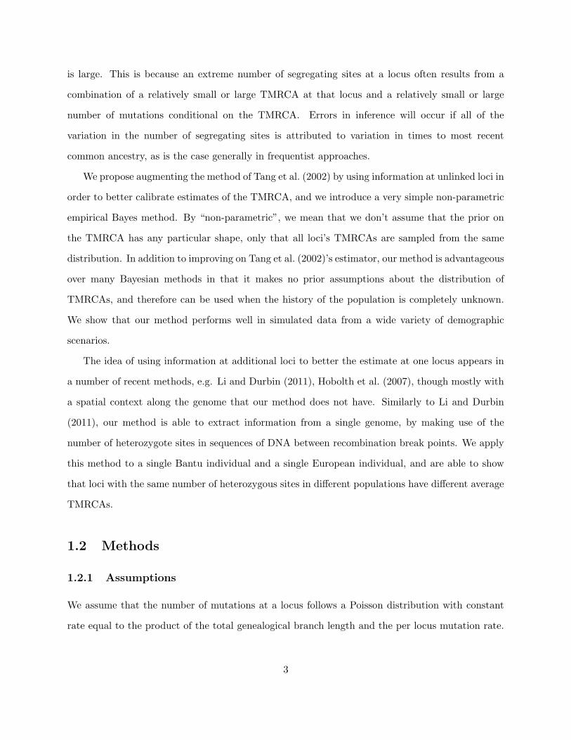
The Ti are in turn independent and identically distributed according to some distribution, which

we do not know and which we do not need to specify. For an illustration of the data generating

process, see figure 1.1.

This data-generating process exactly describes the process that yields the number of mutations

at unlinked loci in a genome, given our assumptions. That is, conditional on Ti and µi`i, each Xi

is an independently distributed Poisson random variable with rate 2µi`iTi, and each Ti is drawn

i.i.d from an unknown distribution. For the sake of computational simplicity, we will assume that

2µi`i = 1, which is equivalent to a simple rescaling of Ti.

Figure 1.1: Data Generating Process for Robbins’ method, in which the distribution P (Ti)is unknown and does not need to be specified.

Under this compound sampling scheme (though initially not applied to genetic data), Robbins

(1955) showed that we can obtain a point estimate of Ti by making use of Bayes’ rule and the form

5

of the Poisson probability distribution:

E[Ti|Xi = xi] =

∫TiP (Ti|xi)dTi =

∫TiP (xi|Ti)P (Ti)

P (xi)dTi

=(xi + 1)

P (xi)

∫e−TiT xi+1

i

(xi + 1)!P (Ti)dTi

=(xi + 1)

P (xi)

∫P (xi + 1|Ti)P (Ti)dTi

=(xi + 1)P (xi + 1)

P (xi),

where P (xi) is the marginal probability that Xi = xi, that is, the marginal probability that we

observed exactly xi segregating sites at locus i. As can be seen from the sampling structure depicted

in Figure 1, this marginal distribution, which we could simply call P (x), does not depend on i.

When the number of loci is not too small, we can approximate P (xi) by the fraction of loci

where the number of observed segregating sites is equal to xi. We use mxi to refer to m times

this fraction, or the number of loci with exactly xi mutations. In this way we obtain the following

estimator of the TMRCA at locus i:

Ti,NPEB = (xi + 1)mxi+1

mxi

. (1.3)

As a note, mutation rates vary across the genome, and we are not assuming a single underlying

mutation rate. Loci with relatively high mutation rates for example can be truncated, such that

the product of the mutation rate and the locus length µi`i across all considered loci is roughly

similar.

Robbins (1955) proved that this estimator is asymptotically optimal. That is, as as the total

number of loci sampled grows (m→∞), its Bayes risk (such as the mean squared error) converges

to the Bayes risk for the Bayesian model where the true prior of the Ti, and therefore P (xi), is

known. As might be expected, Robbins’ method behaves erratically in cases where there are few

data. If for example mxi+1 = 0, that is if no loci have exactly xi + 1 segregating sites, then our

estimate of Ti corresponding to a locus i where there are xi > 0 segregating sites would be 0, which

is clearly wrong. In order to mitigate this effect, there are a number of smoothing techniques one

6

might apply (Gale and Church, 1990, 1994; Lidstone, 1920; Good, 1953). In this paper, we will only

attempt to estimate Ti using Robbins’ method when loci where there are xi segregating sites and

loci where there are xi + 1 segregating sites are not rare. It is indeed for these loci that Robbins’

method shows a clear advantage over traditional methods that do not incorporate information from

other independent loci.

Another consequence of variation in mxi is that estimates of Ti are not necessarily a non-

decreasing function of the number of mutations xi. In fact we would expect loci in which there

are more mutations to be at least as ancient as loci in which there are only a few. In order to

remedy this, we can fit a weighted isotonic regression of the inferred mean Ti,NPEB on the number

of mutations using the pava() function in the “Iso” package (Turner, 2015) in R (R Core Team,

2015) , where we weight each value by

(xi + 1)2m2xi+1

m2xi

(1

mxi

+1

mxi+1

), (1.4)

and obtain a new set of estimators, denoted by TWi,NPEB . We use these weights as an approximation

of the variance of Ti,NPEB , as will be explained in the section entitled “Effectiveness of Robbins’

method”. As the isotonic regression yields the least squares best fit among nondecreasing relation-

ships, performing this step ensures that Ti ≤ Tj if there are fewer mutations at locus i than at

locus j.

To summarize, Robbins’ method uses the ratio of the number of loci with exactly xi and xi + 1

mutations in order to calibrate the TMRCA at a given locus with exactly xi mutations. We

then incorporate the knowledge that the expected number of segregating sites at a locus is a non-

decreasing function of its TMRCA, by running an isotonic regression on the TMRCA estimates.

1.2.4 Generalizing our estimator to a sample of size n ≥ 2

In generalizing our estimator for use on samples of size n ≥ 2, we are inspired by the frequentist

estimation of coalescence times from nucleotide sequence data using a tree-based partition in Tang

et al. (2002). In that work, the n sequences are first partitioned into two subsets which are meant

to correspond to the left and right clades of the genealogical tree. The MRCA of any two sequences,

7

one in the left clade and one in the right clade, is the root of the tree. Tang et al. (2002) propose an

estimator of the TMRCA based on the average number of pairwise differences Di between sequences

in the left clade and sequences in the right clade (see equation 1.1).

Although genealogical trees are not always completely resolved by the data, in many cases there

is little ambiguity about the branching pattern at the root (Tang et al., 2002). When ambiguity

does exist at the root, Tang et al propose a partition algorithm that is less biased than forcing the

pair of sequences that differ most from each other to be in different clades. This algorithm does

not require knowledge of the ancestral state at the segregating sites. The 8 steps of this algorithm

are described in detail in Tang et al. (2002).

We use the following steps to infer Ti in cases where n > 2, which we also illustrate in figure

1.2.

1. For each locus i, where 1 ≤ i ≤ m, we use Tang et al’s tree partitioning algorithm to partition

the sample at locus i into left and right clades.

2. From the set of left-clade samples, we pick at random a single sample. We also pick at random

a sample from the set of right-clade samples. We calculate the number of pairwise differences

and repeat this process for every locus i. The reason we count the number of differences

between single pairs of left-right clade sequences instead of averaging the number of differences

across all left-right clade pairs is that Robbins’ method requires xi to be an integer. We then

calculate a Ti,NPEB for each locus using these counts at all m loci, according to equation

1.3. The result of this step is a table which contains estimates of TMRCA corresponding to

different observed numbers of segregating sites. We then fit a weighted isotonic regression to

these estimates, where each estimate is weighted according to formula 1.4.

3. Clearly, at the end of the previous step, we have not used much of the information from our

sample, as we have sampled only one left-clade right-clade pair from each locus. We therefore

repeat the previous step over all possible left-right clade pairs at a particular locus, which all

have same TMRCA if the partitioning algorithm is correct. For each locus, the number of

possible left-right clade pairs depends on the topology of the tree at that locus. If a single

8

sequence forms one of the clades, the data at that locus will consist of n− 1 highly correlated

pairwise differences. When the tree is balanced, there are (n+1(n is odd))(n−1(n is odd))/4

pairs, many more than in the unbalanced case. We repeat step 2 until all left-right clade pairs

have been used at least once. For loci with the maximum observed number of pairs, each pair

is used exactly once. For loci with fewer pairs, some pairs are used multiple times; these are

sampled uniformly at random after all pairs at a locus have been used once. At the end of

this step, we obtain between n−1 and (n+1(n is odd))(n−1(n is odd))/4 tables, depending

on the m inferred tree configurations. That is, the number of tables produced is equal to the

number of pairs in the locus with the largest amount of left-right pairs.

4. We average the entries in all of the tables obtained in the previous two steps, i.e. the estimates

of TMRCA for each observed number of segregating sites at a locus, and in this way we obtain

a final table with the aggregate information that links each integer-valued unique number of

segregating sites to a unique estimate of the TMRCA.

5. We then consider the data at a single locus i. We calculate Di, the average number of

segregating sites over all left-right clade pairs at this locus. If this average is an integer,

then the estimate of the TMRCA can be read from the row corresponding to value Di in the

final table. More likely than not, though, Di is not an integer. We can create a piecewise

linear function that extends our estimates of the TMRCA to non-integer values of Di. Our

estimate of the TMRCA is then a weighted average of the estimates of the TMRCA in the

rows corresponding to bDic and dDie.

We note here that the presence of recombination does not compromise the method in any way

when n = 2 but does require a reinterpretation of the meaning of the results. The NPEB estimate

will no longer correspond to a single TMRCA at a given locus but to an average TMRCA across

the locus. This is due to the additive properties of the Poisson distribution and to the fact that,

in a sample of size 2, intra-locus recombination will not produce a new tree with a different shape.

Indeed, in a sample of size 2, there is no ambiguity concerning the members of the left and the

right clades. For a sample size greater than 2, we require no intra-locus recombination that affects

9

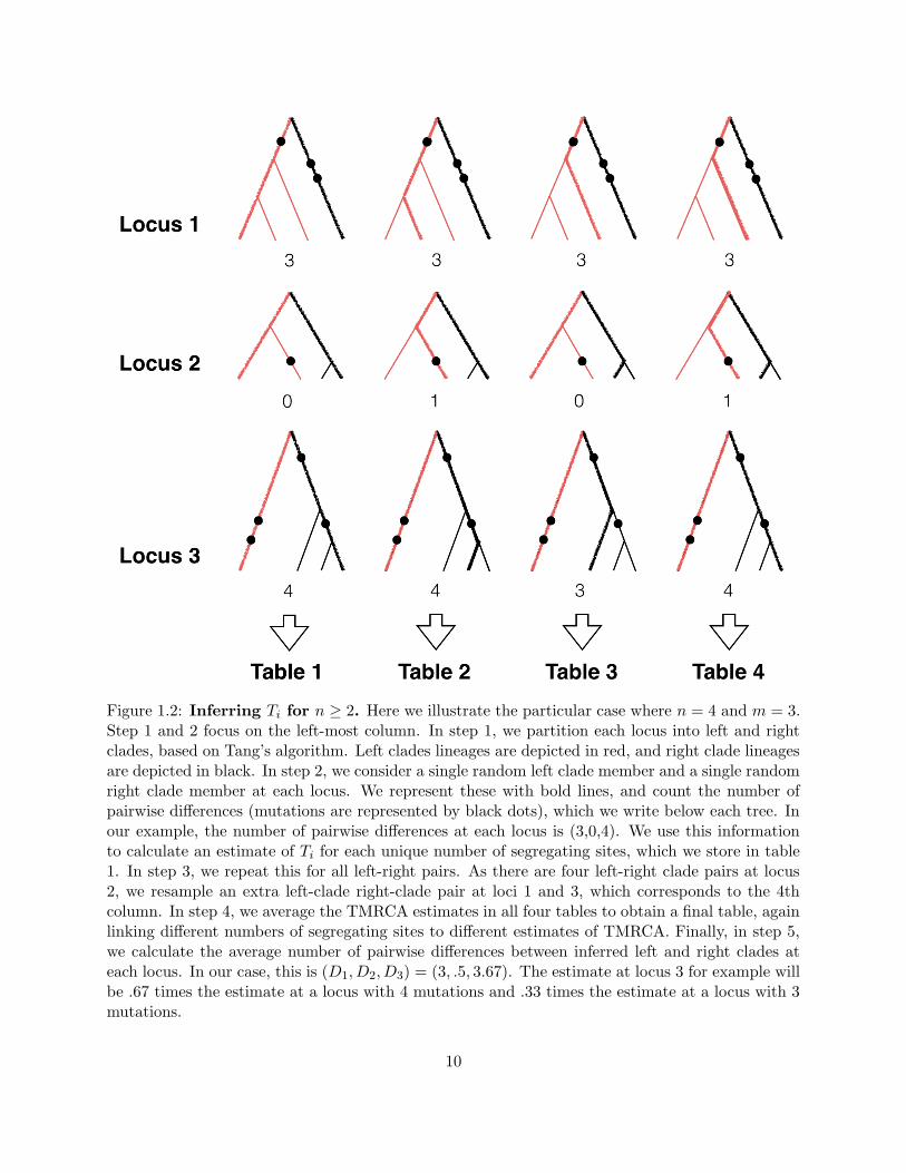
Figure 1.2: Inferring Ti for n ≥ 2. Here we illustrate the particular case where n = 4 and m = 3.Step 1 and 2 focus on the left-most column. In step 1, we partition each locus into left and rightclades, based on Tang’s algorithm. Left clades lineages are depicted in red, and right clade lineagesare depicted in black. In step 2, we consider a single random left clade member and a single randomright clade member at each locus. We represent these with bold lines, and count the number ofpairwise differences (mutations are represented by black dots), which we write below each tree. Inour example, the number of pairwise differences at each locus is (3,0,4). We use this informationto calculate an estimate of Ti for each unique number of segregating sites, which we store in table1. In step 3, we repeat this for all left-right pairs. As there are four left-right clade pairs at locus2, we resample an extra left-clade right-clade pair at loci 1 and 3, which corresponds to the 4thcolumn. In step 4, we average the TMRCA estimates in all four tables to obtain a final table, againlinking different numbers of segregating sites to different estimates of TMRCA. Finally, in step 5,we calculate the average number of pairwise differences between inferred left and right clades ateach locus. In our case, this is (D1, D2, D3) = (3, .5, 3.67). The estimate at locus 3 for example willbe .67 times the estimate at a locus with 4 mutations and .33 times the estimate at a locus with 3mutations.

10

tree shape, because otherwise we could not partition our sample into left and right clades.

1.3 Results

1.3.1 Effectiveness of Robbins’ method

In order to assess where Robbins’ NPEB method is most effective, we calculate the variance of

Ti,NPEB as a function of m, mxi and mxi+1. Using a Taylor expansion, we can approximate the

variance of the ratio of two random variables (Rice, 2007):

Var

(mxi+1

mxi

)≈ (E (mxi+1))

2

(E (mxi))2

(Var (mxi+1)

(E (mxi+1))2 − 2

Cov (mxi ,mxi+1)

E (mxi) E (mxi+1)+

Var (mxi)

(E (mxi))2

). (1.5)

We can represent the distribution of the mxi for each observed xi by a multinomial distribution,

as long as we create a bin to account for all unobserved yet possible values of xi. In the model

there are countably infinite possible numbers of segregating sites, but in practice the number is

limited by `i the length in nucleotides of each locus i. By the properties of the multinomial, we have

E (mxi) = mP (xi), Var (mxi) = mP (xi) (1− P (xi)) and Cov (mxi ,mxi+1) = −mP (xi)P (xi + 1).

Equation 1.5 then simplifies to:

Var

(mxi+1

mxi

)≈ P (xi + 1)2

mP (xi)2

(1

P (xi)+

1

P (xi + 1)

).

Therefore, as Ti,NPEB = (xi + 1)mxi+1

mxi, we have:

Var(Ti,NPEB

)= Var

((xi + 1)

mxi+1

mxi

)≈ (xi + 1)2

P (xi + 1)2

mP (xi)2

(1

P (xi + 1)+

1

P (xi)

). (1.6)

To illustrate where Robbins’ method is most effective, we apply 1.6 to each value xi of an

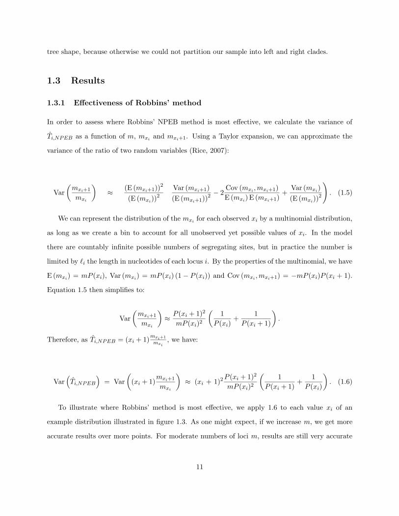
example distribution illustrated in figure 1.3. As one might expect, if we increase m, we get more

accurate results over more points. For moderate numbers of loci m, results are still very accurate

11

if P (xi) is not too small, especially in comparison with P (xi + 1). Finally, the contribution of the

first term on the right side of 1.6 is smallest when xi is small. For these reasons, our method can

give accurate results at sites with xi = 0 segregating sites.

Using the observed data, we can approximate the variance at each point by assuming mxi ≈

mP (xi). This is how we obtain the weights for our isotonic regression (see 1.4).

Figure 1.3: Accuracy of Robbins’ method. For each value of xi, mP (xi) is the expectednumber of sites with exactly xi segregating sites. The bars are shaded and labeled according tothe approximate standard deviation of Ti,NPEB at each locus with xi mutations, obtained usingequation 1.6. There is no estimate of the TMRCA for the locus with 7 mutations, because theNPEB method would require the existence of some number of sites with exactly 8 mutations, andthis is not the case here.

1.3.2 Simulation results in a wide range of population histories

In order to test the performance of our estimator against the traditional frequentist and parametric

Bayesian estimators, we run a series of simulations. Programs sufficient to reproduce all of the

results we present are available at https://wakeleylab.oeb.harvard.edu/resources.

12

We generate synthetic data using the program MSMS (Ewing and Hermisson, 2010), which

generates sequence data and TMRCA values under a range of demographic scenarios including

population growth, subdivision, and admixture. We vary the population mutation rate θ, the

exponential growth rate of the population g, the number of sequences from which we build our

genealogies n, and the divergence time between populations d across a range of parameters described

in table 1.1. We use a cutoff of .2 in step 6 of Tang et al. (2002)’s tree partitioning algorithm. This

essentially disallows sampled pairs that have relatively very few nucleotide differences from being

selected to belong to different tree clades. We choose this value as it is the default setting in Tang

et al. (2002). Note again that we measure time in units scaled by the population mutation rate θ.

We illustrate the performance of the method for two sample sizes, n = 2 and n = 8. Felsenstein

(2006) suggested n = 8 as an optimal choice to balance accuracy of estimating θ against the costs

of genotyping. To justify n = 8, we might also appeal to the results that the expected TMRCA

is equal to 2(1 − 1/n) and that the probability the MRCA of the sample contains the MRCA of

the entire population at a locus is equal to (n − 1)/(n + 1) (Saunders et al., 1984) if the interest

is in the whole-population TMRCA at each locus. Concretely, this means that the TMRCA for 8

lineages is likely to be close to the TMRCA for many more lineages.

For each demographic scenario, we simulate m independent genealogies. We then use our

algorithm to calculate TWi,NPEB at each locus i. To measure performance, we first compute the

mean squared error (MSE) of our estimators at all loci for which our estimate of the variance of

Ti,NPEB is smaller than some threshold, chosen to be 0.1 in these simulations. We will assume that

there are m∗ such loci:

MSEs

(TWi,NPEB

)≈ 1

m∗

∑VarTi,NPEB<0.1

(TWi,NPEB − Ti,T rue)2, (1.7)

where Ti,T rue is the true TMRCA at locus i given by MSMS. The subscript s is the index of one

simulated set of m loci under a given demographic scenario. In order to have a more accurate

estimate of our error, we repeat these simulations S different times for each combination of param-

eters. We then average MSEs over the S different sets in order to obtain the final measure of the

13

accuracy of our estimator, given the demographic scenario.

We impose a cutoff variance because we only expect our method to be advantageous when the

variance of the estimator is reasonably small. That is, it is only beneficial in estimating the TMRCA

of a locus i where mxi and mxi+1 are large. Reasonable values of this threshold will depend on the

population mutation rate θ. The smaller the cutoff variance, the smaller m∗, the number of loci

for we estimate a TMRCA. We specifically chose .1 in these simulations to restrict ourselves to

loci whose TMRCA we could accurately predict, at least more accurately than using Tang et al.

(2002)’s method across the range of parameters in our simulations.

Parameter Values

Number of independent sites m 250, 500, 1000, 2000, 4000Population mutation rate θ 0.25, 0.5, 0.75, 1, 2

Growth rate g 0, 0.5, 1, 2Divergence time d 0, 1, 3

Sample size n 2, 8

Table 1.1: Parameter values in simulations

1.3.3 Comparison to Tang’s method and the parametric Bayes posterior mean

Figure 1.4 is a scatterplot of the MSE of estimates using the method of Tang et al to those obtained

using NPEB for simulations over the parameters in the multi-dimensional grid described in 1.1.

We see that Robbins’ method always performs better than Tang et al.’s approach as measured by

MSE.

As we increase m, our estimates become more and more accurate: the NPEB MSE converges

to the Bayes MSE where the true prior is assumed (Robbins, 1955). We illustrate this for g = 0,

d = 0, n = 2 and .25 < θ < 2.0 in figure 1.5. The parametric Bayes estimates were obtained by

assuming (correctly) that the values Ti were drawn from an exponential distribution with parameter

θ. We update the prior on Ti with the observed number of mutations xi, and in this way obtain

the posterior on Ti. We then report the mean of this posterior (see equation 1.2). For m = 250, the

MSE of the NPEB estimator is, depending on θ, about 3.5 to 7.4 percent higher than the MSE of

the Bayesian estimator using the correct prior. For m = 4000, the difference is even smaller, with

14

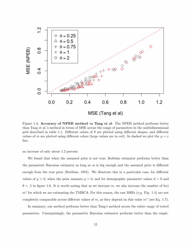
Figure 1.4: Accuracy of NPEB method vs Tang et al. The NPEB method performs betterthan Tang et al.’s method in terms of MSE across the range of parameters in the multidimensionalgrid described in table 1.1. Different values of θ are plotted using different shapes, and differentvalues of m are plotted using different colors (large values are in red). In dashed we plot the y = xline.

an increase of only about 1.2 percent.

We found that when the assumed prior is not true, Robbins estimator performs better than

the parametric Bayesian estimator as long as m is big enough and the assumed prior is different

enough from the true prior (Robbins, 1955). We illustrate this in a particular case, for different

values of g > 0, when the prior assumes g = 0, and for demographic parameter values d = 0 and

θ = .5 in figure 1.6. It is worth noting that as we increase m, we also increase the number of loci

m∗ for which we are estimating the TMRCA. For this reason, the raw MSEs (e.g. Fig. 1.4) are not

completely comparable across different values of m, as they depend on this value m∗ (see Eq. 1.7).

In summary, our method performs better than Tang’s method across the entire range of tested

parameters. Unsurprisingly, the parametric Bayesian estimator performs better than the empir-

15

Figure 1.5: NPEB vs Bayes with true prior assumed. We plot (MSENPEB −MSEBayes)/MSEBayes for different values of m, which we vary in color, and different values ofθ, which we vary in shape. For the parametric Bayes case, we assume as a true prior a constantpopulation size and a divergence time of 0. We use a sample size of 2.

16

ical Bayes estimator when the true prior is assumed. However, our method can outperform the

parametric Bayesian estimate in terms of MSE when the assumes prior is incorrect.

Figure 1.6: NPEB vs Bayes with wrong prior assumed. Here we assume as a prior a constantpopulation size, but in reality the exponential growth rate varies between 0 and 2 (see x-axis). Thevalue of θ is 0.5, and the sample size is 2. Values of m range from 250 (in gray) to 4000 (in red).

1.3.4 Admixture case study

We also consider the special case of admixture, as a more complicated demographic history. In this

case, we can still assume that the true TMRCAs are independent and identically distributed, but

this time according to a more complicated distribution that exhibits bimodality (see figure 1.7).

Using again the program MSMS (Ewing and Hermisson, 2010), we simulate the genealogies of pairs

of just admixed individuals. Their parent populations diverged 6 time units in the past, with 50

percent of the genetic material in the sample originating from the first population and 50 percent

from the second population. This means that 50 percent of sampled lineages will not be able to

17

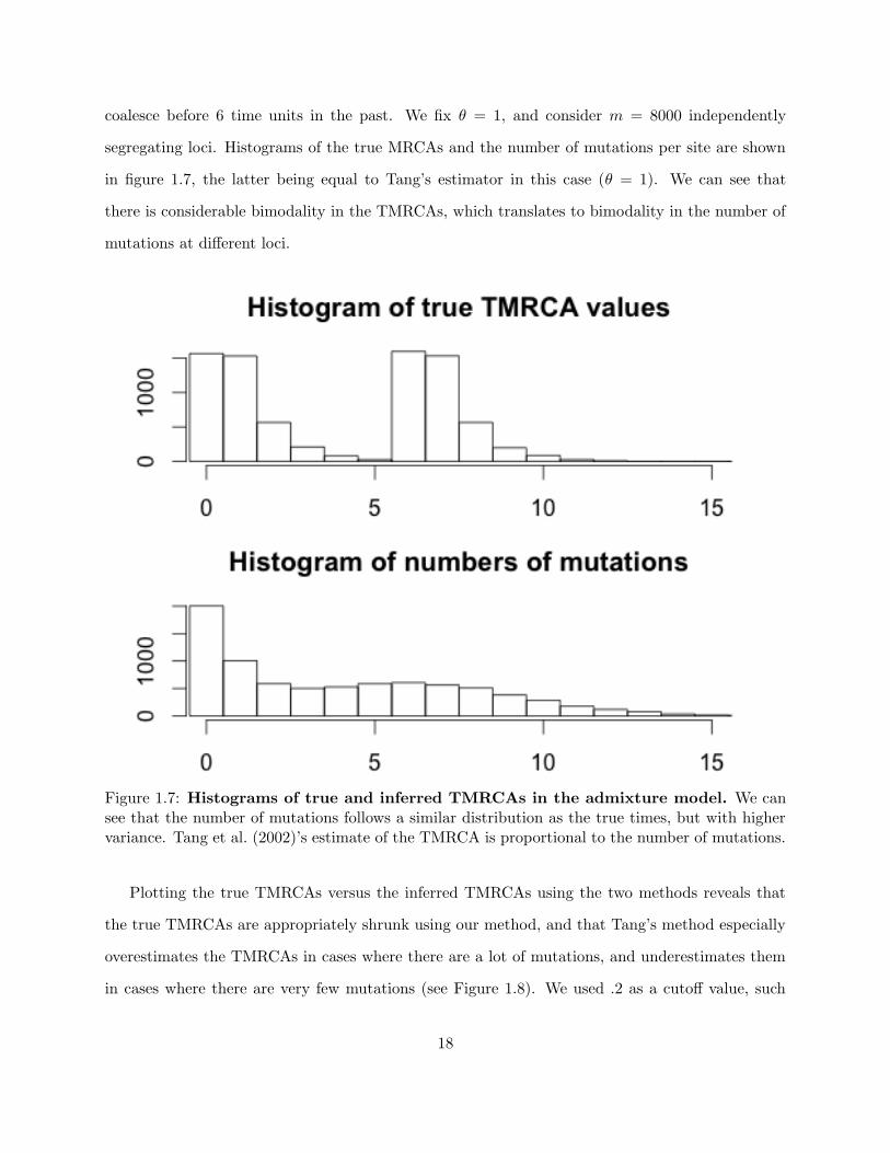
coalesce before 6 time units in the past. We fix θ = 1, and consider m = 8000 independently

segregating loci. Histograms of the true MRCAs and the number of mutations per site are shown

in figure 1.7, the latter being equal to Tang’s estimator in this case (θ = 1). We can see that

there is considerable bimodality in the TMRCAs, which translates to bimodality in the number of

mutations at different loci.

Figure 1.7: Histograms of true and inferred TMRCAs in the admixture model. We cansee that the number of mutations follows a similar distribution as the true times, but with highervariance. Tang et al. (2002)’s estimate of the TMRCA is proportional to the number of mutations.

Plotting the true TMRCAs versus the inferred TMRCAs using the two methods reveals that

the true TMRCAs are appropriately shrunk using our method, and that Tang’s method especially

overestimates the TMRCAs in cases where there are a lot of mutations, and underestimates them

in cases where there are very few mutations (see Figure 1.8). We used .2 as a cutoff value, such

18

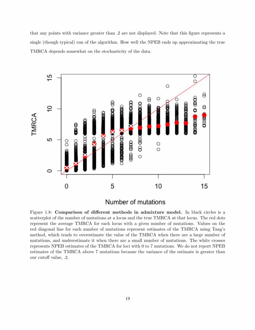
that any points with variance greater than .2 are not displayed. Note that this figure represents a

single (though typical) run of the algorithm. How well the NPEB ends up approximating the true

TMRCA depends somewhat on the stochasticity of the data.

Figure 1.8: Comparison of different methods in admixture model. In black circles is ascatterplot of the number of mutations at a locus and the true TMRCA at that locus. The red dotsrepresent the average TMRCA for each locus with a given number of mutations. Values on thered diagonal line for each number of mutations represent estimates of the TMRCA using Tang’smethod, which tends to overestimate the value of the TMRCA when there are a large number ofmutations, and underestimate it when there are a small number of mutations. The white crossesrepresents NPEB estimates of the TMRCA for loci with 0 to 7 mutations. We do not report NPEBestimates of the TMRCA above 7 mutations because the variance of the estimate is greater thanour cutoff value, .2.

19

1.3.5 Analysis of TMRCAs from human genomes

We also apply our method to data from 37,574 neutrally evolving autosomal loci from a European

and a Bantu individual (Gronau et al., 2011). Each inter-locus distance is at minimum 50,000

base pairs, a distance deemed sufficiently high by Gronau et al. (2011) that the genealogies can

be assumed to be approximately uncorrelated. These presumably neutral loci are 1,000 base pairs

in length, and were chosen to avoid recombination hot-spots. We remove any masked bases, and

reduce all of our loci to 900 base pairs, by truncating loci with greater than 900 unmasked bases

and removing loci with less than 900 unmasked base pairs. We use Gronau et al. (2011)’s estimate

of the mutation rate of 0.7×10−9 mutations per site per year and for the sake of illustration assume

no variation in mutation rate across these loci, which we would otherwise control for by varying

the length of each locus. Because of diploidy, we have a sample of size 2 for each individual.

The distribution of numbers of mutations (or heterozygous sites) is different in the case of the

Bantu and the European (see figure 1.9), which we might attribute to the well-known bottleneck

in the ancestry of European populations (Keinan et al., 2007; Voight et al., 2005). In particular,

the average number of pairwise differences is greater for Bantu than for European. In figure 1.10,

we plot the inferred TMRCA at each locus for each of these two genomes. We notice that, unlike

with our method, the TMRCAs estimated using Tang’s method do not vary depending on the

population. Using our method to estimate TMRCAs, we find that the calibration is less intense

for the European sample than it is for the Bantu sample, which makes sense in light of the fact

that the frequency of sites with exactly xi mutations decreases more sharply as xi increases for the

European sample (figure 1.9).

1.4 Discussion

We have shown that the problem of estimating the TMRCA of a sample can be framed in such a way

that it allows for the use of NPEB methods, such as a modified Robbins’ method. The advantage

of these methods is that they use data from all loci to efficiently account for the randomness of

mutation, through which loci with the same TMRCA can have very different numbers of segregating

20

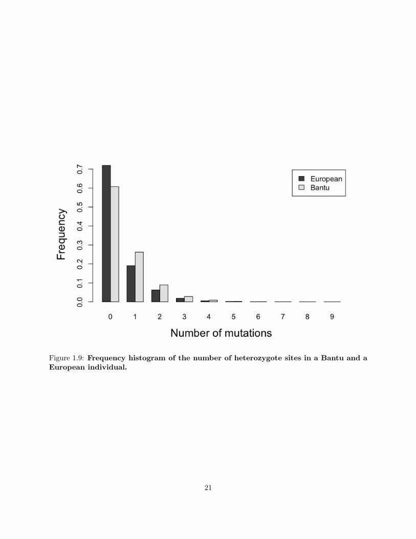
Figure 1.9: Frequency histogram of the number of heterozygote sites in a Bantu and aEuropean individual.

21

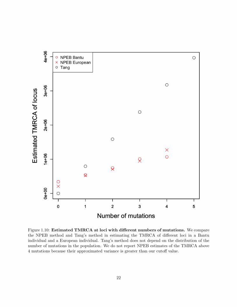
Figure 1.10: Estimated TMRCA at loci with different numbers of mutations. We comparethe NPEB method and Tang’s method in estimating the TMRCA of different loci in a Bantuindividual and a European individual. Tang’s method does not depend on the distribution of thenumber of mutations in the population. We do not report NPEB estimates of the TMRCA above4 mutations because their approximated variance is greater than our cutoff value.

22

sites. In all of our simulations, Robbins’ method, one of the simplest NPEB methods, showed radical

improvement over Tang et al’s maximum likelihood method (this is because the method makes use

of a lot more of the available information). It also performed very well against a parametric Bayesian

method in which it is assumed that the true prior for TMRCA is known.

It is particularly useful in that Robbins’ method provides reliable estimates of the TMRCA

even when the mutation rate is very low. Many of the nucleotide sequences we simulated had

0 segregating sites. Our method was nonetheless reliably able to infer TMRCA at these loci, as

long as there was enough information from other independently segregating loci. The other benefit

of our method is that it does not require any prior assumptions on demographic history. We

ran simulations using simple models of population expansion and divergence and showed that our

method is effective in a wide variety of demographic scenarios.

For all cases where the genealogies uniting the sampled sequences are known, as for example

when the sample is of size 2, the NPEB estimate may be calculated simply and directly using

equation 1.3. However, this method is somewhat limited to loci with sufficiently common numbers

of segregating sites. It does not perform well with outliers, i.e. when mxi is small.

More effective yet complicated NPEB approaches involve estimating the distribution G of the

Ti from the data. Laird (1978) proved that the distribution of Ti that maximizes the likelihood of

the data is a discrete distribution over finitely many points j. An estimate of this distribution can

be obtained using the Expectation-Maximization algorithm (Dempster et al., 1977). We can then

get estimates of each individual Ti by using Bayes rule with G as a prior:

E[Ti|Xi = xi] =

∑j T(j)P (xi|T(j))G(T(j))∑j P (xi|T(j))G(T(j))

. (1.8)

This approach is superior to Robbins’ method in that conditions of monotonicity and convexity

are satisfied, and its success does not depend on the use of a squared error loss function over a

general loss function (Carlin and Louis, 2000). However, it involves much more computation than

Robbins’ method. In this paper, we concentrated on Robbins’ method as our goal was to show that

there is information at independent loci, and that even the simplest NPEB method performs quite

well, especially compared to the maximum likelihood approach.

23

Acknowledgments

We thank N. Rosenberg, P. Ralph, and an anonymous reviewer for very helpful comments.

24

Bibliography

J Brookfield. Importance of ancestral dna ages. Nature, 388:134, 1997.

B Carlin and T Louis. Bayes and Empirical Bayes methods for data analysis. Chapman and Hall

CRC, Boca Raton, 2000.

AP Dempster, NM Laird, and DB Rubin. Maximum likelihood from incomplete data via the EM

algorithm. Journal of the Royal Statistical Society. Series B (Methodological), 39(1):1–38, 1977.

P Donnelly, S Tavar, S Balding, and DJ Griffiths. Estimating the age of the common ancestor of

men from the zfy intron. Science, 272:1357–1359, 1996.

RL Dorit, H Akashi, and W Gilbert. Absence of polymorphism at the zfy locus on the human y

chromosome. Science, 268:1183–1185, 1995.

G Ewing and J Hermisson. MSMS: a coalescent simulation program including recombination,

demographic structure and selection at a single locus. Bioinformatics, 26:2064–2065, 2010.

J Felsenstein. Accuracy of coalescent likelihood estimates: do we need more sites, more sequences,

or more loci? Mol Biol Evol., 23(3):691–700, 2006.

YX Fu and WH Li. Estimating the age of the common ancestor of men from the zfy intron. Science,

272:1356–1357, 1996.

W Gale and K Church. Estimation procedures for language context: poor estimates are worse than

none. COMPSTAT, Proceedings in Computational Statistics, 9:69–74, 1990.

25

William A. Gale and Kenneth W. Church. What’s wrong with adding one? In Corpus-Based

Research into Language. Rodolpi, 1994.

IJ Good. The population frequencies of species and the estimation of population parameters.

Biometrika, 40(3-4):237–264, 1953.

CK Griswold and AJ Baker. Time to the most recent common ancestor and divergence times of

populations of common chaffinches (Fringilla coelebs) in europe and north africa: Insights into

Pleistocene refugia and current levels of migration. Evolution, 56:143–153, 2002.

I Gronau, MJ Hubisz, B Gulko, CG Danko, and A Siepel. Bayesian inference of ancient human

demography from individual genome sequences. Nature Genetics, 43:1031–1034, 2011.

F Hailer, VE Kutschera, BM Hallstrom, D Klassert, SR Fain, and et al. Nuclear genomic sequences

reveal that polar bears are an old and distinct bear lineage. Science, 336:344–347, 2012.

MF Hammer. A recent ancestry for the human y chromosomes. Science, 378:376–378, 1995.

A Hobolth, OF Christensen, T Mailund, and MH Schierup. Genomic relationships and speciation

times of human, chimpanzee, and gorilla inferred from a coalescent hidden markov model. PLoS

Genetics, 3(2):294–305, 2007.

S Jakubiczka, J Arnemann, H Cooke, M Krawczak, and J Schmidtke. A search for restriction

fragment length polymorphism on the human y chromosome. Human Genetics, 84(1):86–88,

1989.

Alon Keinan, James C Mullikin, Nick Patterson, and David Reich. Measurement of the human

allele frequency spectrum demonstrates greater genetic drift in east asians than in europeans.

Nature Genetics, 39:1251–1255, 2007.

N Laird. Nonparametric maximum likelihood estimation of a mixing distribution. Journal of the

American Statistical Association, 73:805–811, 1978.

H Li and R Durbin. Inference of human population history from individual whole-genome sequences.

Nature, 475:493–496, 2011.

26

GJ Lidstone. Note on the general case of the Bayes-Laplace formula for inductive or a posteriori

probabilities. Transactions of the Faculty of Actuaries, 8:182–192, 1920.

R Core Team. R: A Language and Environment for Statistical Computing. R Foundation for

Statistical Computing, Vienna, Austria, 2015. URL https://www.R-project.org/.

J Rice. Mathematical Statistics and Data Analysis, 3rd edition. Duxbury Press, 2007.

H Robbins. An empirical bayes approach to statistics. Proceedings of the Third Berkeley Symposium

on Mathematical Statistics and Probability, 1:157–164, 1955.

NA Rosenberg and MW Feldman. The relationship between coalescence times and population

divergence times. In M Slatkin and M Veuille, editors, Modern Developments in Theoretical

Population Genetics. Oxford University Press, New York, 2002.

I. W. Saunders, S. Tavare, and G. A. Watterson. On the genealogy of nested subsamples from a

haploid population. Adv. Appl. Prob., 16:471–491, 1984.

F Tajima. Evolutionary relationship of DNA sequences in finite populations. Genetics, 105:437–460,

1983.

H Tang, DO Siegmund, P Shen, PJ Oefner, and MW Feldman. Frequentist estimation of coalescence

times from nucleotide sequence data using a tree-based partition. Genetics, 105:437–460, 2002.

Rolf Turner. Iso: Functions to Perform Isotonic Regression, 2015. URL http://CRAN.R-project.

org/package=Iso. R package version 0.0-17.

L Vigilant, M Stoneking, H Harpending, K Hawkes, and A Wilson. African populations and the

evolution of human mitochondrial dna. Science, 253:1503–1507, 1991.

Benjamin F. Voight, Alison M. Adams, Linda A. Frisse, Yudong Qian, Richard R. Hudson, and

Anna Di Rienzo. Interrogating multiple aspects of variation in a full resequencing data set to

infer human population size changes. Proceedings of the National Academy of Sciences of the

United States of America, 102:18508–18513, 2005.

27

Bruce Walsh. Estimating the time to the most recent common ancestor for the y chromosome or

mitochondrial dna for a pair of individuals. Genetics, 158:897–912, 2001.

GA Watterson. On the number of segregating sites in genetical models without recombination.

Theoretical Population Biology, 7:256–276, 1975.

G Weiss and A von Haeseler. Estimating the age of the common ancestor of men from the zfy

intron. Science, 272:1359–1360, 1996.

LS Whitfield, JE Sulston, and PN Goodfellow. Sequence variation of the human y chromosome.

Nature, 378:379–380, 1995.

28

Chapter 2

A non-zero variance of Tajima’s

estimator for two sequences even for

infinitely many unlinked loci

Leandra King, John Wakeley, Shai Carmi

2.1 Introduction

The population mutation rate θ is defined as 4Neµ, where Ne is the effective population size and

µ is the per locus per generation mutation rate. Two classic estimators were developed for θ,

Watterson’s (based on the number of segregating sites (Watterson, 1975)) and Tajima’s (based on

the average number of pairwise differences (Tajima, 1983, 1989)). For a single pair of sequences,

both estimators are identical (denoted here as θ) and equal to the number of differences between

the sequences.

Increasing the number of sampled individuals has limited ability to improve these estimates

of θ, because shared ancestry reduces the number of independent branches where mutations can

arise (Rosenberg and Nordborg, 2002). Felsenstein (2006) showed that the variance of maximum

likelihood estimates of θ decreases approximately logarithmically with the number of individuals

sampled. In contrast, the variance decreases inversely with the number of independent loci. Thus,

29

to increase the accuracy of estimates of θ, it is more effective to increase the number of independent

loci than the sample size at each locus.

Naively, we might consider a set of n unlinked loci, in the sense that they are separated by an

effectively infinitely large recombination rate, to be independent. These loci may be sampled from

the same or different chromosomes. We show here that as n → ∞, the variance of the resulting

estimate of θ does not converge to zero. This behavior results from the fact that coalescence times,

even at unlinked loci, are in fact not independent, but rather weakly correlated. This correlation

is due to Mendelian percolation through the fixed underlying pedigree which is shared by all loci

(Wakeley et al., 2012). In other words, gene genealogies at different loci are constrained by having

to traverse the same common family tree.

The extent of the correlation of coalescence times depends on the sampling configuration, i.e.,

whether the sampled loci are located on the same chromosome, on different homologous chromo-

somes, or on non-homologous chromosomes. This is because the correlation of coalescent times is

induced in part through linkage in the first few generations. In particular, loci sampled from a

same chromosome must have been inherited from the same parent, and loci sampled on different

homologous chromosomes must have originated from different parents. We derive the correlation

analytically using a diploid discrete time Wright-Fisher model (DDTWF), which is an extension

of the haploid DTWF model previously advocated by Bhaskar et al. (2014) for the study of large

samples from finite populations, in which multiple-merger coalescent events might occur.

While the results of the DDTWF model are exact, the dependence on the pedigree is implicit.

For the case of non-homologous chromosomes, we derive an explicit lower bound on the variance

of coalescence times, by taking into account the sharing of genealogical common ancestors across

loci. This calculation, which expands on previous work (Wakeley et al., 2012), provides insight on

how the shape of the gene genealogies is constrained by the underlying pedigree, and on the effect

of these constraints on estimates of the effective population size.

Our results for the variance of θ were obtained under the Wright-Fisher demographic model. To

shed light on the variance of θ under more realistic demographic models, we run simulations based

on real, large-scale human genealogical data (Erlich, 2015). The pedigrees inspired by different

30

human populations differ from each other and from the Wright Fisher pedigrees in a number of

ways, for example in the variance of the relatedness of any two randomly chosen individuals. These

differences lead to differences in the variance of θ for each population, even if they have the same

effective population size.

2.2 The relation of the variance of θ to the correlation of the

coalescence times

For a sample of size two at n loci, the estimator of θ can be expressed as

θ(n) =1

n

n∑i=1

θi, (2.1)

where θi is the number of differences at locus i. If we assume the loci are exchangeable, we have:

Var[θ(n)

]=

Var[θi

]n

+n− 1

nCov

[θi, θj

]. (2.2)

This variance corresponds to the variation expected among independent outcomes of the evolu-

tionary process, including the population pedigree. Under the standard coalescent model (Kingman,

1982), θi is Poisson distributed with mean 2µTi, where Ti is the time until coalescence at locus i in

generations and µ is the mutation rate per locus per generation. Using the law of total covariance,

Cov[θi, θj

]= E

[Cov

[θi, θj |Ti, Tj

]]+ Cov

[E[θi|Ti, Tj

],E[θj |Ti, Tj

]]= 4µ2Cov [Ti, Tj ] , (2.3)

since conditional on Ti and Tj , θi and θj are independent. Thus,

Var[θ]

= limn→∞

Var[θ(n)

]= 4µ2Cov [Ti, Tj ] . (2.4)

31

Because Ti is distributed exponentially with rate 1/(2Nd) under the standard coalescent model

(Kingman, 1982; Tajima, 1983), Var [Ti] = 4N2e . Since Cov [Ti, Tj ] = Corr [Ti, Tj ]×Var [Ti], we can

write:

Var[θ]

= (4µNe)2Corr [Ti, Tj ] , (2.5)

or

Corr [Ti, Tj ] = Var[θ]/[E[θ]]2

(2.6)

and we focus henceforth on the correlation of Ti and Tj . Studying the correlation instead of the

covariance also allows us later on to visually compare the results across different effective population

sizes.

2.3 The effect of the sampling configuration

We now describe the six sampling configurations for a pair of unlinked loci in a sample of two

sequences (Figure 2.1). Four of these sampling configurations involve a sample of two individuals,

and we start by describing these.

In the first configuration, the loci are located effectively infinitely far apart on the same chromo-

some in both individuals. This means that these loci will be coupled for the first few generations,

until separated by a recombination event. Once separated, they may later back-coalesce onto the

same chromosome, and again resume percolating together through the pedigree for a period of

time that is expected to be short. (In the event of back-coalescence, two ancestral loci not sharing

genetic material come to be located on the same chromosome, which essentially undoes the effect

of recombination.) In the second configuration, the loci are on different homologous chromosomes,

meaning they will necessarily be present in different parents in the immediately preceding genera-

tion, as each chromosome was inherited from a different parent. It is then also possible for them

to back-coalesce in later generations. The third configuration is a mixture of the first two: the loci

are located on the same chromosome in one individual, and on homologous chromosomes in the

other. In the fourth configuration, the loci are sampled from non-homologous chromosomes in both

individuals. This configuration is different from the previous three in that back-coalescence is not

32

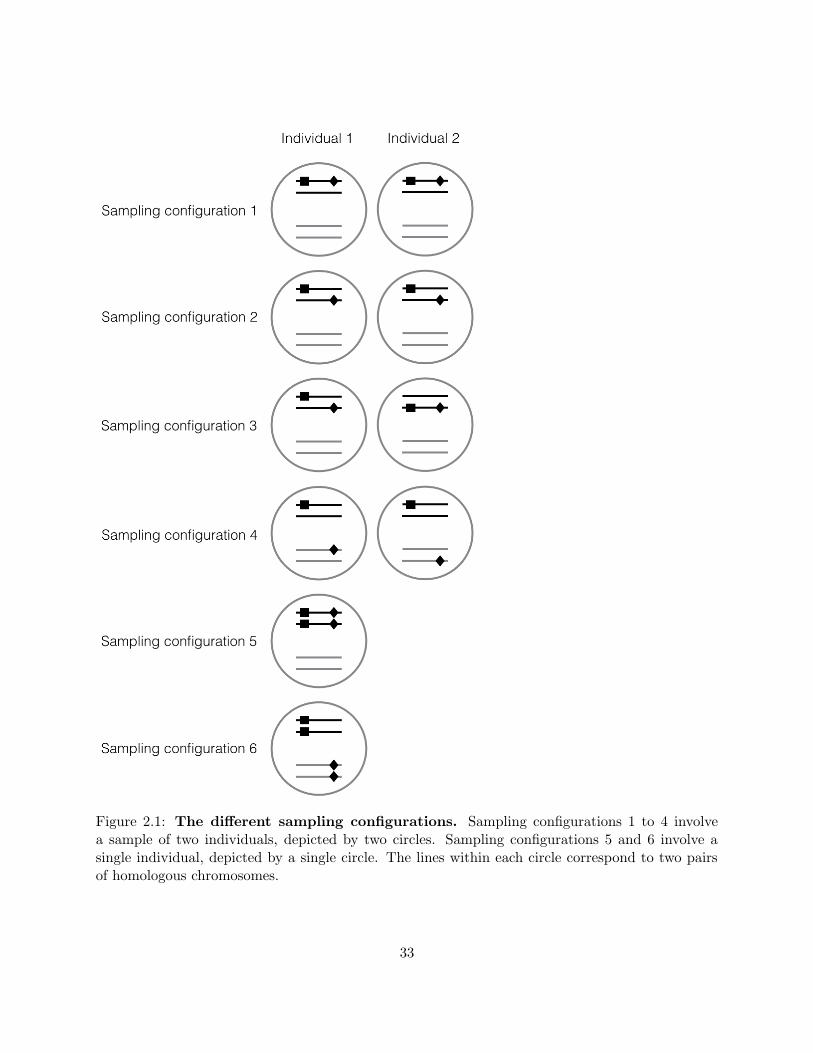
Figure 2.1: The different sampling configurations. Sampling configurations 1 to 4 involvea sample of two individuals, depicted by two circles. Sampling configurations 5 and 6 involve asingle individual, depicted by a single circle. The lines within each circle correspond to two pairsof homologous chromosomes.

33

possible.

In the fifth and sixth sampling configurations, all sequences are sampled from a single indi-

vidual. This is common in applications, in part because measuring the heterozygosity in a single

individual does not require haplotype phasing. In configuration 5, we sample two loci from the

same chromosome (and their pairs from the homologous chromosome). Given that each homolo-

gous chromosome must originate from a different parent, in one generation the sampled loci will

transition to configuration 1 with probability 0.25, to configuration 2 with probability 0.25, and to

sampling configuration 3 with probability 0.5. In sampling configuration 6, the sampled loci are

on different (non-homologous) chromosomes. This configuration is reduced in one generation to

sampling configuration 4, and therefore has the same correlation properties as that configuration.

2.3.1 The DDTWF model

To study the correlation of coalescence times under the different sampling configurations, we use

a DTWF model. This class of models has been advocated as an alternative to the coalescent

when the sample size is large relative to the population size, as it can accommodate multiple and

simultaneous mergers (Bhaskar et al., 2014).

In our case, we assume non-overlapping generations, a constant population size of Ne diploid

individuals, half of which are male and half of which are female, random mating between the sexes,

no selection, and no migration. There are three possible types of events: recombination, coalescence,

and back-coalescence. Because the population size is finite, combinations of these events can occur

in a single generation. We also keep track of whether lineages are in the same individual or not, as

this determines their trajectory in the immediately preceding generation. We refer to this model

as the 2-sex DDTWF. Later we will consider a simplified (1-sex) DDTWF. The dynamics of this

2-sex DDTWF model can be summarized by a Markov transition matrix (Supplementary Material

section 2.8.2) with 17 states, where the initial state is one of the sampling configurations 1, 2, 3,

or 5.

This model is indeed only designed for pairs of loci sampled from either the same chromosome or

homologous chromosomes, as the notions of back-coalescence and recombination only make sense

34

when this is the case. However, by modifying the interpretation of the states of the transition

matrix, we can also model sampling configurations 4 and 6, which involve non-homologous chromo-

somes. This is because recombination for unlinked loci is indistinguishable from loci simply being

located on two chromosomes inherited from the same parent but from different grandparents in

terms of the path these loci take through the pedigree.

Given this transition matrix, we can write a system of equations using first step analysis for all

states x such that E[TiTj |x] > 0:

E[TiTj |x] =∑k

pxkE[(Ti + 1)(Tj + 1)|k]

= 1 +∑k

pxkE[Ti|k] +∑k

pxkE[Tj |k] +∑k

pxkE[TiTj |k]

= E[Ti|x] + E[Tj |x] +∑k

pxkE[TiTj |k]− 1, (2.7)

where pxk is the transition probability between states x and k.

Solving this system of equations allows us to obtain exact results for Cov [Ti, Tj |x]. As a note,

E[Ti|x] can be different than E[Tj |x] depending on the state x. For example, if the pair of lineages

at locus i is located on two different chromosomes in the same individual, whereas the pair of

lineages at locus j is located in two different individuals, then E[Ti|x] = E[Tj |x] + 1. To obtain

the correlation, we can then normalize this covariance by the variance of the time until MRCA

at a locus, which is the same regardless of whether the lineages were sampled from a same or

from different individuals. This variance can also be calculated using the aforementioned system

of equations with i = j.

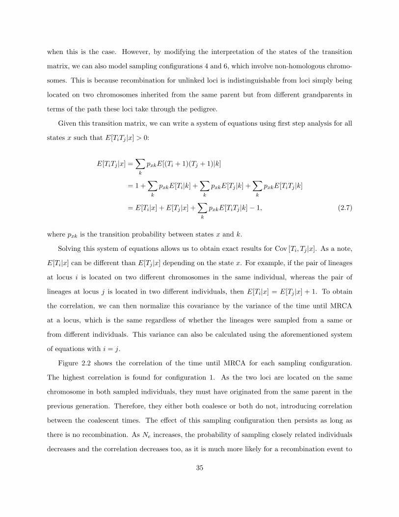
Figure 2.2 shows the correlation of the time until MRCA for each sampling configuration.

The highest correlation is found for configuration 1. As the two loci are located on the same

chromosome in both sampled individuals, they must have originated from the same parent in the

previous generation. Therefore, they either both coalesce or both do not, introducing correlation

between the coalescent times. The effect of this sampling configuration then persists as long as

there is no recombination. As Ne increases, the probability of sampling closely related individuals

decreases and the correlation decreases too, as it is much more likely for a recombination event to

35

Figure 2.2: Correlation of coalescent times for a sample of size 2. These correlationswere calculated for different sampling configurations using the 2-sex DDTWF and the simplifiedDDTWF (described in detail in Supplementary Section 2.8.2). The different configurations in thelegend are associated with the corresponding states of the Markov Chain, written in curly brackets,as described in the supplement.

occur before a coalescence event. Sampling configuration 3 (two loci located far apart on the same

chromosome in one individual, and on different chromosomes in the second individual) shows the

lowest correlation. In fact, it is slightly negative for very small values of Ne, for if one of the loci

coalesces in the first generation, then it is impossible for the other locus to coalesce. The correlation

in other configurations is intermediate between those of configurations 1 and 3.

In figure 2.2, we also show the results from a simplified DDTWF model. This model is similar

to the 2-sex DDTWF, except that individuals are monoecious and we do not keep track of whether

lineages are in the same individual or not. There are much fewer states in this model than in the

2-sex DDTWF, and it is therefore significantly easier to analyze. The simplified model turns out

as a very good approximation to the 2-sex DDTWF, even for moderately large Ne. More details

on both models are given in Supplementary Material sections 2.8.2.

36

2.4 The effect of the shared pedigree

The 2-sex DDTWF model allows us to calculate exactly the correlation of coalescence times at

two loci. In this section, we aim to provide more intuition with regard to the role of the shared

underlying pedigree in generating positive correlations of coalescent times.

2.4.1 Inconsistency of θ due to the underlying pedigree

The value of θ is a function of the pedigree that connects the two individuals in our sample, where

the pedigree itself is randomly drawn from from a demographic model (e.g., the Wright-Fisher

model). If the sampled individuals happen to be more closely related than average, then θ will

tend to underestimate the true value of θ. The opposite is true if the sampled individuals are less

closely related than average.

Let δ be the probability that a randomly sampled pair of individuals is very closely related, for

example as full siblings. Let ε be some arbitrary value smaller than the difference between θ and

θ∗, where θ∗ is estimated from a sample of full siblings. By sampling sufficiently many loci (or gene

genealogies), we could theoretically infer the common ancestry of the sampled pair to any desired

accuracy. However, this would not give information about the pedigree beyond the ancestry of the

sampled pair, and as the sampled pair is related more closely than average, θ∗ would underestimate

θ. For this fixed ε and δ, we therefore cannot find n large enough such that Prob(|θ∗(n)−θ| > ε) < δ.

This implies that there is no convergence in probability, which means that this estimate of θ is not

consistent. In turn, this inconsistency implies that the variance of θ(n) does not tend to 0 as n

increases.

As a note, since the pedigree itself is the product of a stochastic model (Wright-Fisher or

otherwise), even a fully specified pedigree leaves uncertainty regarding the value of θ. In other

words, the uncertainty in the estimate of θ results from having at hand only a single sample from

a single pedigree generated from a stochastic model that is governed by that parameter (see also

Ralph (2015)).

37

2.4.2 A lower bound on the limiting variance

Here, we analytically calculate a lower bound on the limiting variance of θ in the case of non-

homologous chromosomes, in a way that provides an intuitive understanding of the effect of the

shared pedigree. We compute the covariances of Ti and Tj by conditioning on a vector of variables

{x} = x1, x2, ..., xG, where xg is the number of shared ancestors g generations ago. This vector

{x} is in a sense a lower dimensional representation of the shared pedigree, and can be used to

approximate the probability of coalescence each generation. For example, if x1 = 2 (full siblings),

then all loci have the same 25% probability of coalescing within a single generation. We only

consider the first G = log2N generations, where N is the (constant) effective population size, as

it was shown that the effect of the shared pedigree is important only up to ≈ log2N generations

(Wakeley et al., 2012; Derrida et al., 2000; Chang, 1999). Beyond that time, almost all ancestors

are shared, and the distribution of the contributions of each ancestor to the present day sample is

approximately stationary.

By the law of total covariance, we have:

Cov [Ti, Tj ] = E{x} [Cov [Ti, Tj |{x}]]

+ Cov{x} [E [Ti|{x}] ,E [Tj |{x}]] . (2.8)

E{x} [Cov [Ti, Tj |{x}]] ≈ 0, because conditioning on the pedigree, the loci are independently segre-

gating. Therefore:

Cov [Ti, Tj ] = Cov{x} [E [Ti|{x}] ,E [Tj |{x}]]

= Var{x} [E [Ti|{x}]] . (2.9)

To compute E [Ti|{x}], we condition on whether coalescence has occurred in the first G generations.

If it has not occurred, we assume that the process then behaves just as the standard coalescent, or

38

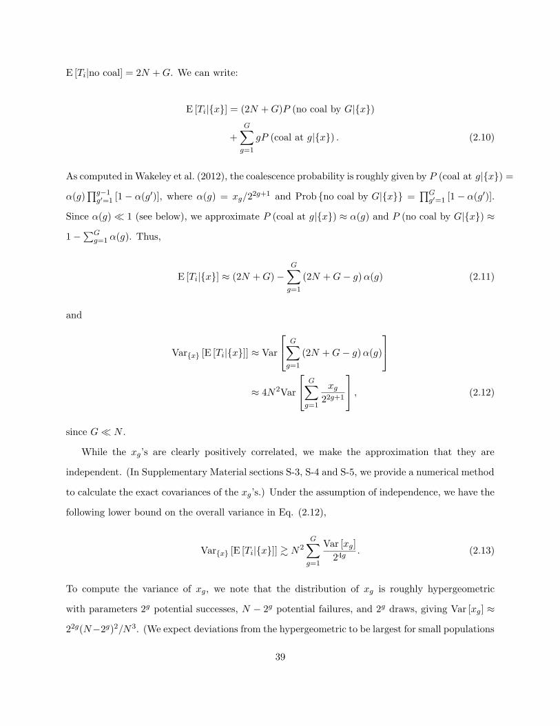
E [Ti|no coal] = 2N +G. We can write:

E [Ti|{x}] = (2N +G)P (no coal by G|{x})

+G∑g=1

gP (coal at g|{x}) . (2.10)

As computed in Wakeley et al. (2012), the coalescence probability is roughly given by P (coal at g|{x}) =

α(g)∏g−1g′=1 [1− α(g′)], where α(g) = xg/2

2g+1 and Prob {no coal by G|{x}} =∏Gg′=1 [1− α(g′)].

Since α(g)� 1 (see below), we approximate P (coal at g|{x}) ≈ α(g) and P (no coal by G|{x}) ≈

1−∑G

g=1 α(g). Thus,

E [Ti|{x}] ≈ (2N +G)−G∑g=1

(2N +G− g)α(g) (2.11)

and

Var{x} [E [Ti|{x}]] ≈ Var

G∑g=1

(2N +G− g)α(g)

≈ 4N2Var

G∑g=1

xg22g+1

, (2.12)

since G� N .

While the xg’s are clearly positively correlated, we make the approximation that they are

independent. (In Supplementary Material sections S-3, S-4 and S-5, we provide a numerical method

to calculate the exact covariances of the xg’s.) Under the assumption of independence, we have the

following lower bound on the overall variance in Eq. (2.12),

Var{x} [E [Ti|{x}]] & N2G∑g=1

Var [xg]

24g. (2.13)

To compute the variance of xg, we note that the distribution of xg is roughly hypergeometric

with parameters 2g potential successes, N − 2g potential failures, and 2g draws, giving Var [xg] ≈

22g(N−2g)2/N3. (We expect deviations from the hypergeometric to be largest for small populations

39

sizes, because the number of ancestors in generation g is less than 2g more often in very recent

generations in small populations. We provide the exact distribution of the variance of xg in the

Supplement sections S4, S5 and S6). Substituting in Eq. (2.13),

Var{x} [E [Ti|{x}]] &1

Ne

G∑g=1

(N − 2g)2

22g. (2.14)

Using G = log2N , we have∑G

g=1(N−2g)2

22g= (N

2

3 − 2N + 3 logNlog 8 + 5

3) ≈ N2

3 for large N , and hence,

using Eq. (2.9),

Cov [Ti, Tj ] &N

3. (2.15)

Using Eq. (2.4) and θ = 4µN , we finally obtain

Var[θ]&

θ2

12N. (2.16)

In summary, the variance due to the shared pedigree adds a term of order at least θ2/N ,

independently of the number of regions n. Thus, as argued in the previous section, even for a large

number of chromosomes the variance does not decay to zero, but rather to a constant that depends

on the effective population size.

2.5 Simulations

2.5.1 Wright-Fisher simulations

In this section, we use simulated data to support our analytical results from sections 2.3.1 and

2.4.2. To estimate the correlation of coalescence times at two loci, we first simulate many Wright-

Fisher pedigrees and sample two individuals from the current generation for each pedigree. We set

the population size N to be the same in every generation, with equal numbers of males and fe-

males. We then consider two loci on non-homologous chromosomes and simulate the path through

the pedigree connecting the two lineages at each locus to their MRCA. In each generation and

for each locus, lineages that are found in the same individual coalesce with probability 1/2, in

40

Figure 2.3: The total correlation of the time until MRCA at unlinked loci sampled from non-homologous chromosomes across different Wright-Fisher pedigrees is plotted in green, along withthe analytic lower bounds for the pedigree-induced correlation calculated in Eq. (2.15).

which case the coalescence time is recorded. Loci on different chromosomes in the same individ-

ual neither coalesce in that generation nor in the previous generation. We repeat this process

multiple times for each pedigree to obtain an estimate of E [T |ped]. We then compute its vari-

ance over many simulated pedigrees to obtain Varped [E [T |ped]]. By the same logic as Eq.(2.9)

above, Varped [E [T |ped]] is equal to Cov [Ti, Tj ]. To obtain the correlation, we divide Cov [Ti, Tj ]

by Var [T ] = Varped [E [T |ped]] + Eped [Var [T |ped]].

The total correlation calculated by simulating over many Wright-Fisher pedigrees is exactly

equivalent to the results from the 2-sex DDTWF. The lower bound in Eq. (2.16) combined with

Eq.(2.6), result in the bound Corr [Ti, Tj ] & 1/(12N). This approximate result is also well supported

by simulations, as illustrated in Figure 2.3.

2.5.2 Simulations based on real pedigrees

The Wright-Fisher model is only one way to generate pedigrees under a given effective population

size. Real human pedigrees have complex structures that depend on the geographical region. For

41

example, there are different rates of consanguineous marriages in different countries (Bittles and

Black, 2015), different distributions of the number of children per family, and different mating

structures (leading to differences in the number of full-siblings and half-siblings). To gain insight

on the effect of these differences on the ability to estimate θ, we construct a Wright-Fisher-like

model, but which is constrained by patterns of real human pedigrees. Specifically, we use the

Familinx database, compiled by Erlich (2015), which carries information on about 44 million

individuals from different countries.

We extracted genealogical data for three countries (Kenya, Sweden, USA) from Familinx. We

then used these data to simulate pedigrees by breaking down and reassembling small family units,

as previously described for a different dataset (Wakeley et al., 2012). Specifically, we first split

the genealogies into two-generational family units of children and their parents. To belong to

a unit, a child must share at least one parent with at least one other child in the family unit.

Because Familinx contains data on more than the three countries we chose, in order not to create

a bias in favor of smaller, simpler family units, we only require that the first sampled child be in

the corresponding country data set. These family units then serve as building blocks to generate

pedigrees with the same mating patterns and distribution of the number of children as in the

reference population. We generated pedigrees with a pre-specified effective population size Ne in

a range from 20 to 140. The census population size that corresponds to this Ne was determined

by simulation for each country by averaging the time until coalescence across randomly sampled

pairs and across pedigrees. Clearly, some information is lost in breaking large genealogies into

family units, such as inter-generational correlations in family size, or the rate of first and second

cousin matings. Nevertheless, sufficient information is captured so that pedigrees with the same Ne

built using data from different countries can be distinguished based on the correlation of coalescent

times. Once the pedigrees were generated, we simulated genealogies through those pedigrees as

described in section 2.5.1. Additional details on the simulations are provided in the Supplement

section S1.

For each country and Ne, we then use the simulated data to compute the correlation of coa-

lescence times, as in section 2.5.1 (i.e., Varped [E [T |ped]] divided by Var [T ]). The results (Figure

42

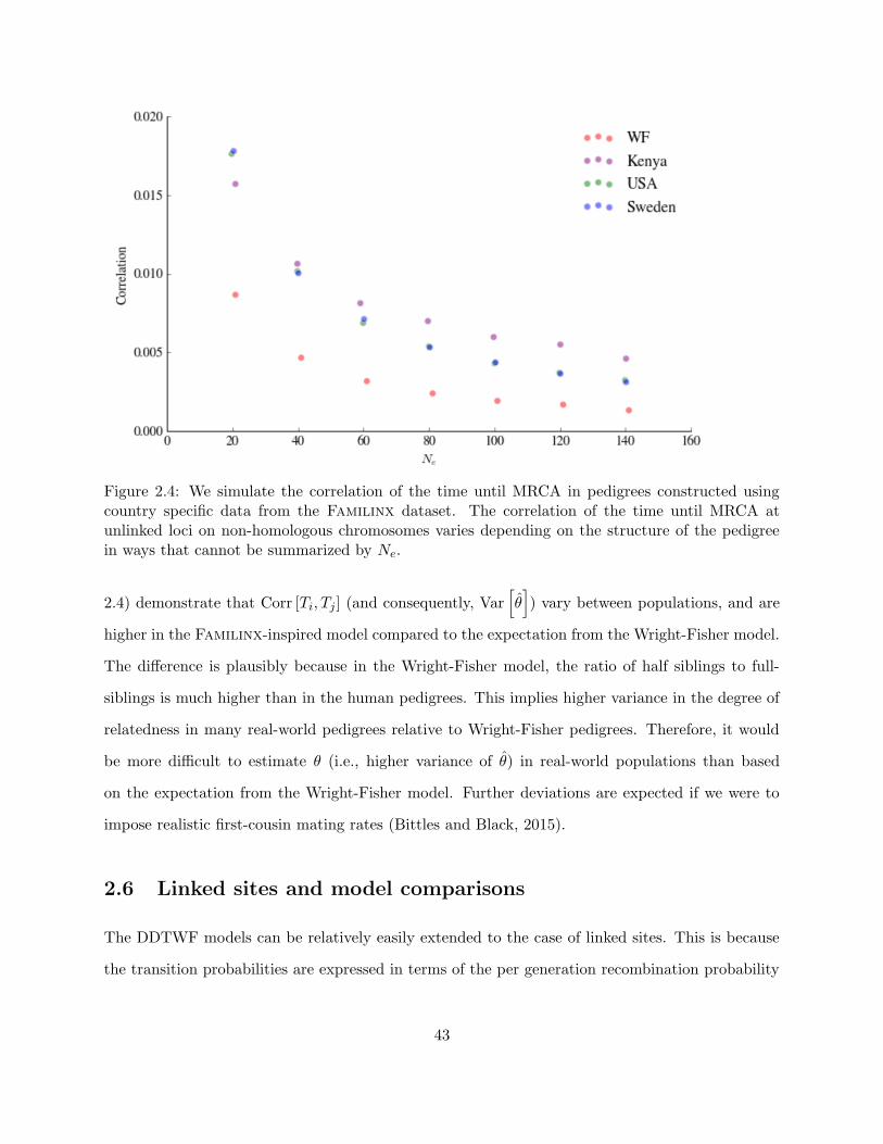
Figure 2.4: We simulate the correlation of the time until MRCA in pedigrees constructed usingcountry specific data from the Familinx dataset. The correlation of the time until MRCA atunlinked loci on non-homologous chromosomes varies depending on the structure of the pedigreein ways that cannot be summarized by Ne.

2.4) demonstrate that Corr [Ti, Tj ] (and consequently, Var[θ]) vary between populations, and are

higher in the Familinx-inspired model compared to the expectation from the Wright-Fisher model.

The difference is plausibly because in the Wright-Fisher model, the ratio of half siblings to full-

siblings is much higher than in the human pedigrees. This implies higher variance in the degree of

relatedness in many real-world pedigrees relative to Wright-Fisher pedigrees. Therefore, it would

be more difficult to estimate θ (i.e., higher variance of θ) in real-world populations than based

on the expectation from the Wright-Fisher model. Further deviations are expected if we were to

impose realistic first-cousin mating rates (Bittles and Black, 2015).

2.6 Linked sites and model comparisons

The DDTWF models can be relatively easily extended to the case of linked sites. This is because

the transition probabilities are expressed in terms of the per generation recombination probability

43

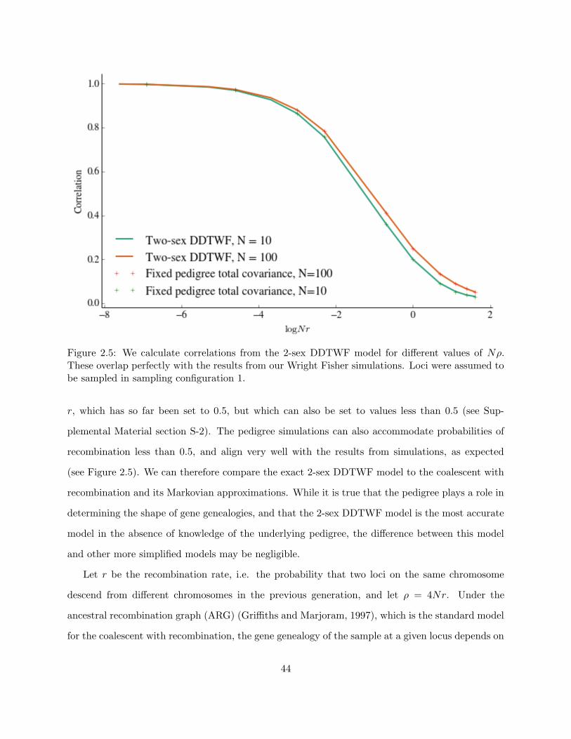
Figure 2.5: We calculate correlations from the 2-sex DDTWF model for different values of Nρ.These overlap perfectly with the results from our Wright Fisher simulations. Loci were assumed tobe sampled in sampling configuration 1.

r, which has so far been set to 0.5, but which can also be set to values less than 0.5 (see Sup-

plemental Material section S-2). The pedigree simulations can also accommodate probabilities of

recombination less than 0.5, and align very well with the results from simulations, as expected

(see Figure 2.5). We can therefore compare the exact 2-sex DDTWF model to the coalescent with

recombination and its Markovian approximations. While it is true that the pedigree plays a role in

determining the shape of gene genealogies, and that the 2-sex DDTWF model is the most accurate

model in the absence of knowledge of the underlying pedigree, the difference between this model

and other more simplified models may be negligible.

Let r be the recombination rate, i.e. the probability that two loci on the same chromosome

descend from different chromosomes in the previous generation, and let ρ = 4Nr. Under the

ancestral recombination graph (ARG) (Griffiths and Marjoram, 1997), which is the standard model

for the coalescent with recombination, the gene genealogy of the sample at a given locus depends on

44

all previous genetic ancestries along the sequence (Wiuf and Hein, 1999). The covariance satisfies

(e.g., Simonsen and Churchill (1997)),

CovARG [Ti, Tj ] =18 + ρ

18 + 13ρ+ ρ2. (2.17)

In contrast, under the Sequentially Markov Coalescent (SMC) (McVean and Cardin, 2005),

each new genealogy (following recombination) depends only on the previous genealogy, and the

new coalescence time must differ from the previous time (no back-coalescence allowed). In this

case, we have:

CovSMC [Ti, Tj ] =1

1 + ρ. (2.18)

The SMC’ model (Marjoram and Wall, 2006) is a variant of SMC where back-coalescence is allowed.

Under SMC’ (Eriksson et al., 2009; Wilton et al., 2015),

CovSMC’ [Ti, Tj ] = 2ρ/2e−ρ/4(−ρ)−1/2−ρ/4 (2.19)

×[Γ

(2 + ρ

4

)+ Γ

(2 + ρ

4,−ρ

4

)].

The covariances of coalescent times derived from the ARG, the SMC, and the SMC’ are expected to

be equal to the correlations of coalescent times (because Ti and Tj are assumed to be exponentially

distributed with rate 1). In Figure 2.6, we compare the correlation of Ti and Tj as a function of ρ

for different values of Ne and r across the different models. Compared to the full 2-sex DDTWF

model, the simplified DDTWF is an extremely good approximation even for Ne as small as 100.

The maximum difference in correlation between these two models across the range of values of ρ

in Figure 2.6 was less than .005. Therefore, the simplified model may be preferred due its much

reduced complexity (see also figure 2.2). The ARG also provides a very good approximation under

these conditions. In turn, the SMC’ model shows slight deviations compared to the ARG, while, as

previously shown, the SMC model deviates more substantially (Wilton et al., 2015). For N = 10,

we observe a small but noticeable difference between the 2-sex and simplified DDTWF models,

where the maximal difference in correlation is around .025, and between these models and the

45

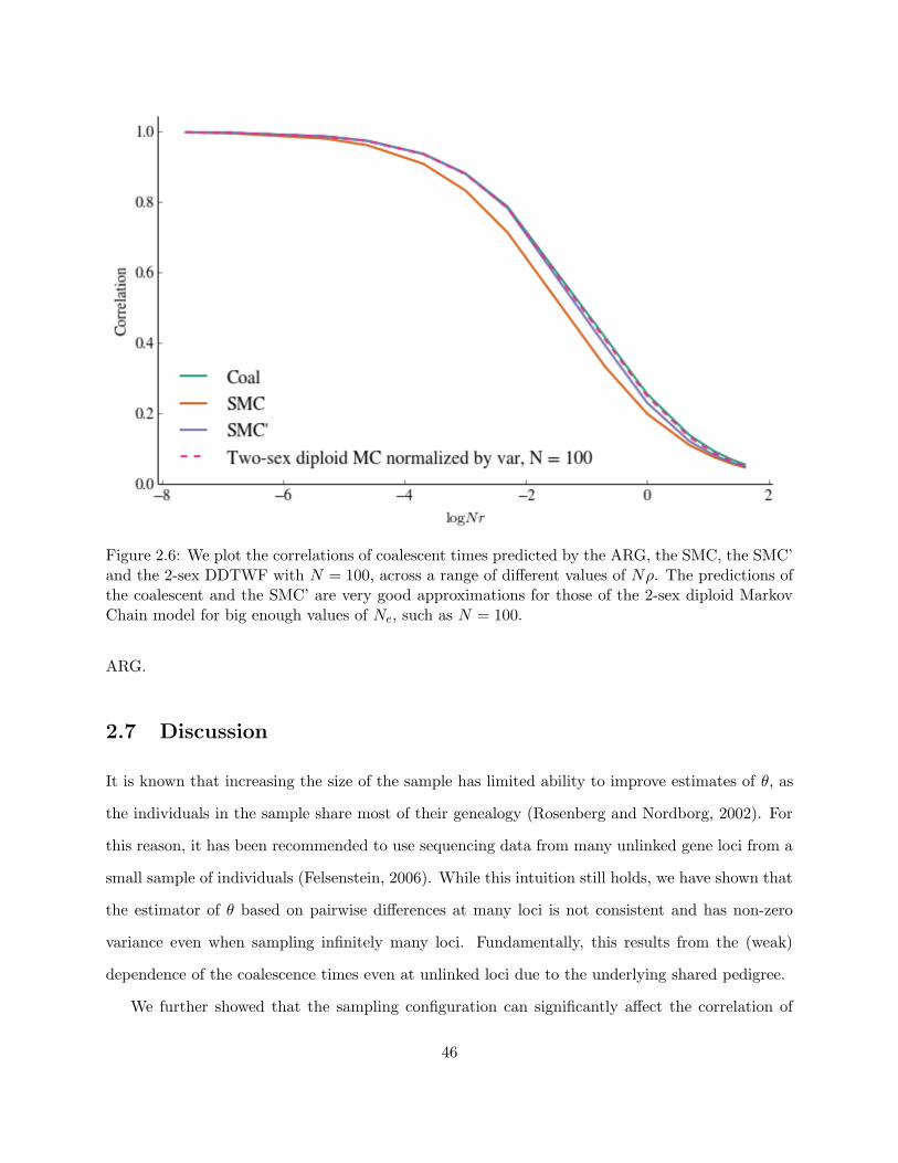
Figure 2.6: We plot the correlations of coalescent times predicted by the ARG, the SMC, the SMC’and the 2-sex DDTWF with N = 100, across a range of different values of Nρ. The predictions ofthe coalescent and the SMC’ are very good approximations for those of the 2-sex diploid MarkovChain model for big enough values of Ne, such as N = 100.

ARG.

2.7 Discussion

It is known that increasing the size of the sample has limited ability to improve estimates of θ, as

the individuals in the sample share most of their genealogy (Rosenberg and Nordborg, 2002). For

this reason, it has been recommended to use sequencing data from many unlinked gene loci from a

small sample of individuals (Felsenstein, 2006). While this intuition still holds, we have shown that

the estimator of θ based on pairwise differences at many loci is not consistent and has non-zero

variance even when sampling infinitely many loci. Fundamentally, this results from the (weak)

dependence of the coalescence times even at unlinked loci due to the underlying shared pedigree.

We further showed that the sampling configuration can significantly affect the correlation of

46

coalescence times, as it restricts the number of available gene genealogies for each pair of loci. We

studied in detail the possible ways by which two loci could be sampled from two sequences and

computed the correlation of the coalescence times for each configuration.

Even with sampling configurations where loci can truly travel independently through the pedi-

gree, we still observe positive correlation across loci. This is because the pedigree that connects

any pair of individuals is invariant across loci, inducing correlation between the coalescence times

at those loci. We used this view to obtain a lower bound on the covariance of coalescence times,

by explicitly conditioning the number of ancestors the two individuals share in the first few gen-

erations. The shared pedigree itself is assumed to be a single draw from a random demographic

process (Wright-Fisher or another), with some characteristic effective population size. Even if we

were able to perfectly characterize the single pedigree at hand, we cannot hope to infer with com-

plete certainty the parameters of the demographic model. It is worth noting, however, that one can

adopt a different (philosophical) view, under which the pedigree itself is the subject of inference,

and is not a product of a random demographic process (Ralph, 2015). Under such a view, there

are no estimators of θ (or of an effective population size).

The analytical results in this paper are based on the Wright-Fisher model. To gain insight on

the behavior of more realistic demographic models, we adapted the Wright-Fisher model according

to the family structure of real human populations. The results demonstrated that the correlation

of coalescence times is higher in the human-inspired models than in the WF model; therefore, θ

should be more difficult to estimate than expected under the pure WF model.

The existence of a detailed pedigree for the sample at hand can be useful when studying the pop-

ulation dynamics (e.g., Moreau et al. (2011)) without resorting to somewhat arbitrary demographic

models. When using models, it is not always clear whether it is necessary to retain all features of

the real population (two sexes, diploidy, etc.), or whether a simplified model could display similar

characteristics. We used our analytical framework to study the correlation of coalescence times as

a function of the scaled recombination rate ρ for the 2-sex and the simplified DDTWF models, and

compared the results to the coalescent with recombination and its Markovian approximations. We

found that as expected, unless the effective population size is extremely small (N ≤ 10), the results

47

for the coalescent (as well as its SMC’ approximation, but not SMC) were extremely close to those

of the DDTWF models. In contrast, differences were observed for N = 10, even between the 2-sex

and the simplified DDTWF.

Finally, we have focused on a sample of two individuals at two loci. For unlinked loci, we

showed that the variance of θ for any number of loci is reduced to the two-loci problem. Extending

the sample size to more than two individuals is expected to be significantly more complicated.

Deviations between the coalescent and the discrete time haploid Wright-Fisher model for increasing

sample sizes were recently studied and shown to be important for realistic human demographic

histories (Bhaskar et al., 2014). We similarly expect the presence of a shared pedigree to have an

increasingly significant effect on the variance of Tajima’s estimator as the sample size grows, but

this analysis is left for future studies.

48

2.8 Extended methods and analytical results

2.8.1 Building pedigrees with Familinx

We simulate our pedigree over GEN = 100 non-overlapping generations. For each generation, we

select at random family units from the data until the total number of children across all of these

family units is greater than some pre-determined N , and the total number of parents is less than or

equal to N . Then, we connect the GEN generations together by randomly assigning each parent

in generation g to be one of the children in generation g + 1, disallowing sibling mating. Finally

we connect the first and last generation so that the pedigree is cyclical with a period of GEN

generations.

As a note, this procedure will not be appropriate for datasets where a substantial number of

family units contain only one child because the algorithm requires a number of children greater

than or equal to the number of parents. Families with many children will be over-sampled, and

the family structure of the constructed pedigrees will be very different from the family structure

we are attempting to replicate.

The value of N was determined to correspond on average to a certain target effective population

size Ne. We estimate the Ne for each constructed pedigree by simulating the average time until

coalescence over 50 sampled pairs. We discard pedigrees whose estimated effective population size

is not within σNe of the target Ne, where σNe is the standard deviation of the observed coalescent

effective sizes for a population of size N = Ne in the Wright-Fisher model. We constrain our

pedigrees to be close to the target effective population size because we want to make sure that

the higher total covariance we observe in the Familinx pedigree simulations relative to the Wright

Fisher is not only due to potentially higher variance of Ne.

2.8.2 The DDTWF models

The 2-sex DDTWF transition matrix

The notation we use to label the states in the 2-sex DDTWF transition matrix is derived from the

notation of Wakeley and Lessard (2003), who built a similar transition matrix to analyze patterns

49

2-sex diploid DTWF model

State coal 1,1 2,2 (1,1) (2,2) 1,1, (1,1), 1,1, (1,2), (1, 1), (1,2), 12,1, (12,1), (12,2), 12, 12, 12 (12, 12)2,2 2, 2 (2,2) 1, 2 (2, 2) (1,2) 2 2 1 (1,2)

coal 1 0 0 0 0 0 0 0 0 0 0 0 0 0 0 0 01,1 1 1 0 1 0 0 0 0 0 0 0 0 0 0 0 0 02,2 1 0 1 0 1 0 0 0 0 0 0 0 0 0 0 0 0(1,1) 0 1 0 0 0 0 0 0 0 0 0 0 0 0 0 0 0(2,2) 0 0 1 0 0 0 0 0 0 0 0 0 0 0 0 0 01,1,2,2 1 1 1 1 1 1 1 1 1 1 1 1 1 1 1 1 1(1,1), 2,2 0 1 0 0 0 1 0 1 1 0 1 1 0 1 1 1 01,1,(2,2) 0 0 1 0 0 1 1 0 1 0 1 1 1 0 1 1 0(1,2), 1,2 1 1 1 1 1 1 1 1 1 1 1 1 1 1 1 1 0(1,1),(2,2) 0 0 0 0 0 1 0 0 1 0 1 1 0 0 1 1 0(1,2),(1,2) 1 1 1 1 1 1 1 1 1 1 1 1 0 0 1 1 012,1,2 1 1 1 1 1 0 0 0 1 1 1 1 1 1 1 1 1(12,1),2 0 1 0 0 0 0 0 0 0 0 0 1 0 1 1 1 0(12,2),1 0 0 1 0 0 0 0 0 0 0 0 1 1 0 1 1 012, (1,2) 0 1 1 0 0 0 0 0 1 0 0 1 1 1 0 0 012,12 1 0 0 1 1 0 0 0 0 0 1 0 0 0 1 1 1(12,12) 0 0 0 0 0 0 0 0 0 0 1 0 0 0 1 1 0

Table 2.1: 2-sex diploid DTWF model. The cell at coordinates (i, j) is 1 if the probability oftransitioning to state j starting from state i in one generation is non-zero.

of linkage disequilibrium in a 2-locus multi-deme model. We detail this notation in supplementary

figure 2.7.

Consider two copies of a first locus, ‘1’, located in two different individuals. On the same chro-

mosomes as the copies of this first locus are copies of a second locus, ‘2’. This is our sampling state,

which we represent as {12,12}. The comma separates the different chromosomes on which there is

followed genetic material. We distinguish this state from {(12,12)}, the parentheses indicating that

the followed pairs of loci are present on two different chromosomes in the same individual. If the

followed lineages are on different chromosomes in the same individual, then they must be located

in different individuals in the previous generation. So, for example, state {(1,1)} (which is the state

where the two copies of locus ‘2’ have coalesced, and the two copies of locus ‘1’ are in the same

individual on different chromosomes) automatically transitions to state {1,1} in one generation.

The set of all possible states in our model is : {}, {1,1}, {2,2}, {(1,1)}, {(2,2)}, {1,1,2,2},

{(1,1),2,2}, {1,1,(2,2)}, {1,2,(1,2)}, {(1,1),(2,2)}, {(1,2),(1,2)}, {12,1,2}, {(12,1),2}, {(12,2),1},

{12,(1,2)}, {12,12} and {(12,12)}. We show the communicating states in this transition matrix

in table 2.1.

50

Figure 2.7: States of the 2-sex DDTWF model. Circles represent individuals; the two lineswithin each individual represents a pair of homologous chromosomes; the square represent thefirst followed locus and the diamond represents the second followed locus. {12,12} corresponds tosampling configuration 1, and is the sampling state we use to calculate correlations of coalescenttimes.

51

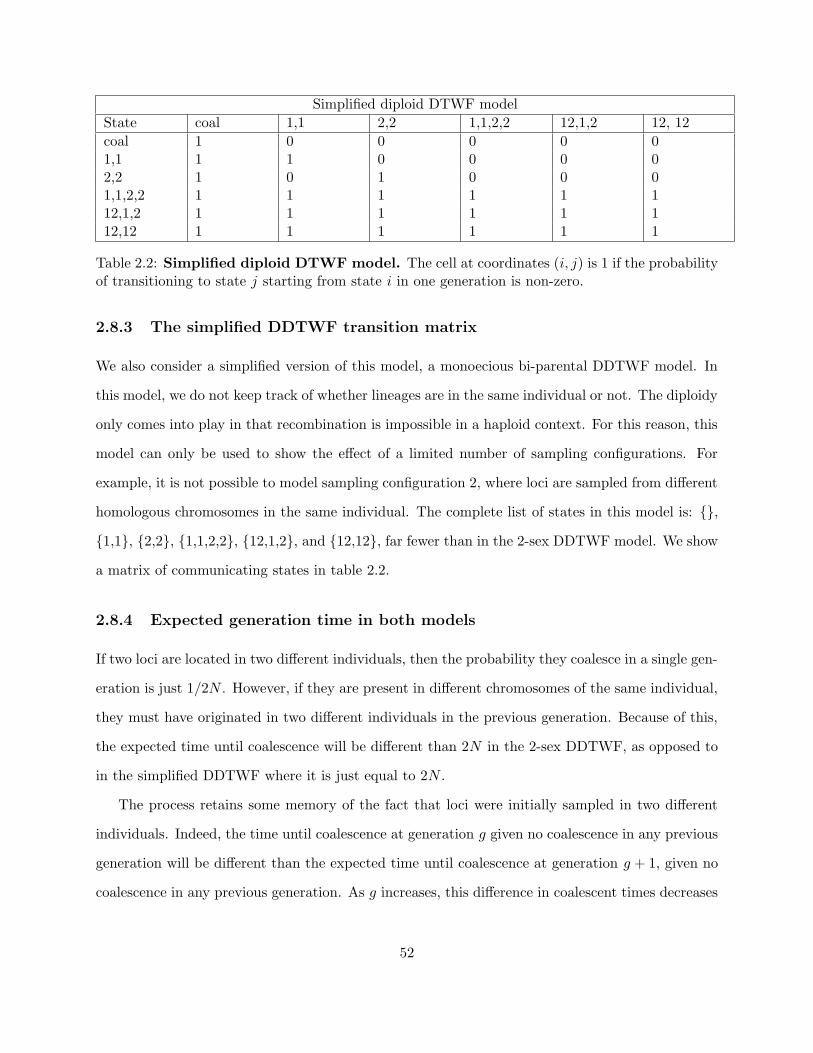
Simplified diploid DTWF model

State coal 1,1 2,2 1,1,2,2 12,1,2 12, 12

coal 1 0 0 0 0 01,1 1 1 0 0 0 02,2 1 0 1 0 0 01,1,2,2 1 1 1 1 1 112,1,2 1 1 1 1 1 112,12 1 1 1 1 1 1

Table 2.2: Simplified diploid DTWF model. The cell at coordinates (i, j) is 1 if the probabilityof transitioning to state j starting from state i in one generation is non-zero.

2.8.3 The simplified DDTWF transition matrix

We also consider a simplified version of this model, a monoecious bi-parental DDTWF model. In

this model, we do not keep track of whether lineages are in the same individual or not. The diploidy

only comes into play in that recombination is impossible in a haploid context. For this reason, this

model can only be used to show the effect of a limited number of sampling configurations. For

example, it is not possible to model sampling configuration 2, where loci are sampled from different

homologous chromosomes in the same individual. The complete list of states in this model is: {},

{1,1}, {2,2}, {1,1,2,2}, {12,1,2}, and {12,12}, far fewer than in the 2-sex DDTWF model. We show

a matrix of communicating states in table 2.2.

2.8.4 Expected generation time in both models

If two loci are located in two different individuals, then the probability they coalesce in a single gen-

eration is just 1/2N . However, if they are present in different chromosomes of the same individual,

they must have originated in two different individuals in the previous generation. Because of this,

the expected time until coalescence will be different than 2N in the 2-sex DDTWF, as opposed to

in the simplified DDTWF where it is just equal to 2N .

The process retains some memory of the fact that loci were initially sampled in two different

individuals. Indeed, the time until coalescence at generation g given no coalescence in any previous

generation will be different than the expected time until coalescence at generation g + 1, given no

coalescence in any previous generation. As g increases, this difference in coalescent times decreases

52

from one generation to the next, and the process converges to an average generation time.

Consider a sampled pair of genes in two individuals. In generation g+1, given that no coalescent

events occurred in any of the previous g generations, the probability that the two followed lineages

coalesce is

C(g + 1) =1

4P (F (g)|No Coal) +

1

8P (H(g)|No Coal),

where P (F (g)|No Coal) and P (H(g)|No Coal) are the probabilities that the two lineages are

located in full siblings and half siblings respectively in generation g, given no coalesce in that

generation or any of the previous generations. In addition, we have

P (F (g)|No Coal) =1− 2C(g)

1− C(g)

1

(N/2)2,

where the term 1 − 2C(g) is the probability that the two lineages are in different individuals,

and the denominator 1 − C(g) arises because we are conditioning on no coalescence in generation

g. The probability that two lineages located in different individuals share exactly two parents is

1(N/2)2

. In the same way, we have:

P (H(g)|No Coal) =1− 2C(g)

1− C(g)

2

N/2

N/2− 1

N/2,

By solving C(g + 1) = C(g), we obtain the limiting coalescent probability as a function of N .

As the distribution of the time until MRCA follows a geometric distribution, the generation time

is the inverse of the probability of coalescence each generation, or

E[Ti] =2N

1 +N −√

1 +N2.

This generation time is always slightly greater than 2N . E[Ti]2N quickly converges to 1 as N

becomes large.

53

2.8.5 Distribution of the number of ancestors from one generation to the next

Consider a single individual in the population with non-overlapping generations in a 2-sex model.

Each generation g, there are Nfg males and Nmg females. Let yg be the number of ancestors of a

particular individual at generation g in the past. During the first few generations, the number of

ancestors grows very fast, and we expect yg ≈ 2g. As the number of ancestors in a given generation

starts to approach the size of the population, the ancestors overlap with one another, and the

growth of ancestors slows down until an equilibrium distribution is reached. We are interested in

modeling the exact distribution of the number of ancestors in generation g + 1, yg+1, given the

number of ancestors in generation g, yg.

We can first divide the number of ancestors in generation g + 1 into males and females:

yg+1 = F +M,

where F is the number of fathers of individuals in yg, and M is the number of mothers of individuals

in yg.

We have

P (F = f |yg) =

(Nf(g+1)

f

)f !S2(yg, f)

(Nf(g+1))yg

where S2 is the Stirling number of the second kind. The intuition behind this formula is that

there are(Nf(g+1)

f

)possible ways of choosing f fathers among the Nf(g+1) available. There are

then f ! possible orderings of these chosen males. The Stirling number of the second kind is the

number of ways we can partition a set of yg individuals into f categories. We divide all this by the

total number of ways of making yg choices of fathers among the Nf(g+1) available, or (Nf(g+1))yg .

Likewise,

P (M = m|yg) =

(Nm(g+1)

m

)m!S2(yg,m)

(Nm(g+1))yg .

We then obtain the following convolution for the number of ancestors a in generation g + 1:

P (yg+1 = a|yg) =

a−1∑f=1

P (F = f |yg)P (M = a− f |yg).

54

y1, ..., yG form a Markov Chain. Using the preceding formula, we can create a transition matrix

yg+1 given yg.

If we didn’t have a two sex model, but instead a bi-parental monoecious model, the formula for

the number of ancestors in generation g + 1 would be the following simpler expression:

P (yg+1 = a|yg) =

(Na

)a!S2(2yg, a)

N2ygg+1

.

2.8.6 Overlap in the number of ancestors each generation

In the previous section, we described the distribution of the number of ancestors each generation.

Here, we start with a sample of size 2 individuals, A and B, and are interested in the distribution of

the number of shared ancestors each generation. If this sample consists of a pair of full siblings, then

the number of shared ancestors grows according to the formula provided in the previous section,

as full siblings share all of their ancestors in common.

Let Xg be the set of common ancestors in generation g. Let Ag be the ancestors of A that are

not in Xg, and Bg be the set of ancestors of B that are not in Xg. Let |Ag|, |Bg| and |Xg| be the

cardinality of these three disjoint sets.

Let FA be the set of fathers of individuals in Ag, and let |FA| be the cardinality of FA. Likewise

we define FX , FB, |FX |, and |FB|. Given |Ag|, |Bg| , and |Xg|, the distribution of |FA|, |FB|, and

|FX | is as described in the previous section. That is, we have:

P

(|FA| = f

∣∣∣∣Ag) =

(Nf

)f !S2(|Ag|, f)

N|Ag |f(g+1)

,

P

(|FB| = f

∣∣∣∣Bg) =

(Nf

)f !S2(|Bg|, f)

N|Bg |f(g+1)

,

and

P

(|FX | = f

∣∣∣∣Xg

)=

(Nf

)f !S2(|Xg|, f)

N|Xg |f(g+1)

.

The number of fathers in common between individuals in Ag and Xg, xa, follows a hypergeo-

metric distribution with FX success states, Nf(g+1) − |FX | failure states, and |FA| draws:

55

P (|FA ∩ FX | = xa) =

(|FX |xa

)(Nf(g+1)−|FX ||FA|−xa

)(Nf(g+1)

|FA|) .

The probability that individuals in Bg have xb fathers in common with individuals in Xg, and

ba fathers in common with individuals in Ag, given that |FA ∩ FX | = xa, is defined by a trivariate

hypergeometric distribution:

P

(|FB ∩ FX | = xb and |FB ∩ FA| = ab

∣∣∣∣|FA ∩ FX | = xa

)=

(|FX |xb

)(|(FA−FX∩FA|ab

)(Nf(g+1)−|(FX∪FA)||FB |−xb−ab

)(Nf(g+1)

|FB |) .

The number of shared male ancestors in generation g + 1 is |Xf(g+1)| = |FX |+ ab, the number

of male ancestors exclusive to A is |Af(g+1)| = |FA| − ab − xa, and the number of male ancestors

exclusive to B is |Bf(g+1)| = |FB| − ab− xb.

To obtain the number of shared female ancestors, Xm(g+1), we use the same protocol, except

replacing Nf(g+1) by Nm(g+1). Finally, to derive the joint distribution of Xg+1, Ag+1 and Bg+1, we

take the convolution over the number of male and female ancestors.

In this way, we can derive a transition matrix T . The entries Tij of the transition matrix give

the probability of entering state j = (|Ag+1|, |Bg+1|, |Xg+1|) given state i = (|Ag|, |Bg|, |Xg|).

We plot the dynamics of the number of shared ancestors every generation in figure 2.8. The

distribution of the number of shared ancestors in generation g is obtained by considering the g-th

power of T , assuming a sampling configuration of (1, 1, 0) and then summing over the probabilities

of all configurations with same |Xg|.

If instead of having a two sex model, we simply had a bi-parental model, then the distribution

of the possible configurations in generation g+ 1, given the configuration in generation g would be:

P (|KB∩KX | = xb and |KB∩KA| = ab | |KA∩KX | = xa) =

(|KX |xb

)(|(KA−KX∩KA)|ab

)(N(g+1)−|(KX∪KA)||KB |−xb−ab

)(N(g+1)

|KB |) ,

where KA, KB and KX are the parents of individuals in Ag, Bg, and Xg respectively.

56

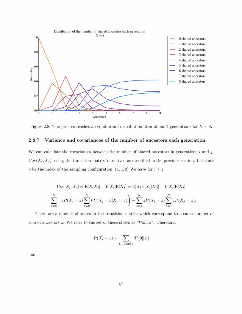
Figure 2.8: The process reaches an equilibrium distribution after about 7 generations for N = 8.

2.8.7 Variance and covariances of the number of ancestors each generation

We can calculate the covariances between the number of shared ancestors in generations i and j,

Cov(Xi, Xj), using the transition matrix T , derived as described in the previous section. Let state

0 be the index of the sampling configuration, (1, 1, 0) We have for i ≤ j:

Cov[Xi, Xj ] = E[XiXj ]− E[Xi]E[Xj ] = E[XiE[Xj |Xi]]− E[Xi]E[Xj ]

=N∑z=0

(zP (Xi = z)

N∑k=0

kP (Xj = k|Xi = z)

)−

N∑z=1

zP (Xi = z)N∑z=1

zP (Xj = z).

There are a number of states in the transition matrix which correspond to a same number of

shared ancestors z. We refer to the set of these states as “Conf z”. Therefore,

P (Xi = z) =∑

zi∈Conf z

T i[0][zi]

and

57

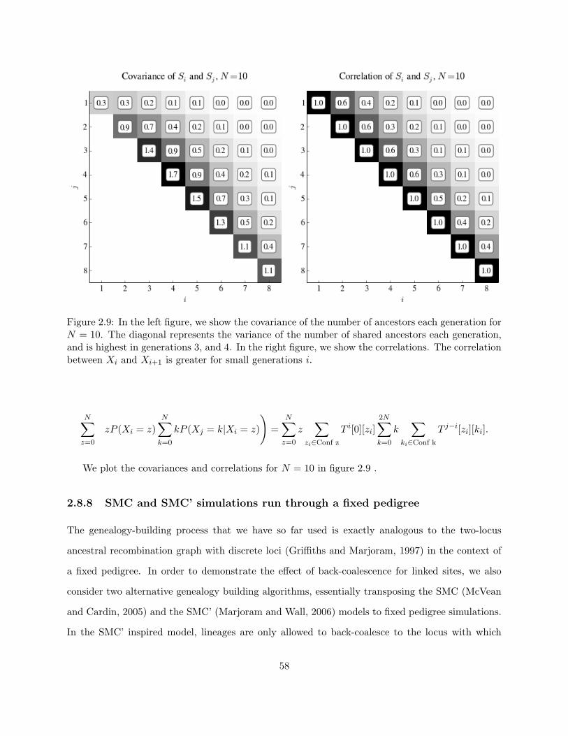
Figure 2.9: In the left figure, we show the covariance of the number of ancestors each generation forN = 10. The diagonal represents the variance of the number of shared ancestors each generation,and is highest in generations 3, and 4. In the right figure, we show the correlations. The correlationbetween Xi and Xi+1 is greater for small generations i.

N∑z=0

(zP (Xi = z)

N∑k=0

kP (Xj = k|Xi = z)

)=

N∑z=0

z∑

zi∈Conf z

T i[0][zi]2N∑k=0

k∑

ki∈Conf k

T j−i[zi][ki].

We plot the covariances and correlations for N = 10 in figure 2.9 .

2.8.8 SMC and SMC’ simulations run through a fixed pedigree

The genealogy-building process that we have so far used is exactly analogous to the two-locus

ancestral recombination graph with discrete loci (Griffiths and Marjoram, 1997) in the context of

a fixed pedigree. In order to demonstrate the effect of back-coalescence for linked sites, we also

consider two alternative genealogy building algorithms, essentially transposing the SMC (McVean

and Cardin, 2005) and the SMC’ (Marjoram and Wall, 2006) models to fixed pedigree simulations.

In the SMC’ inspired model, lineages are only allowed to back-coalesce to the locus with which

58

they were previously linked. That is, no lineage shuffling is allowed. In the SMC inspired model, it

is not possible to back-coalesce at all (Holboth and Jensen, 2013). In all of these simulations, any

amount of assorting of the genetic material in between the two followed loci is ignored.

In the context of the fixed pedigree, the SMC can be seen as a mixture of sampling configuration

1 and sampling configuration 4. Indeed, the loci are sampled in configuration 1. They travel

together until a recombination event occurs, at which point they may no longer back-coalescence.

After a recombination event, the loci behave as if they were sampled in configuration 4.

The SMC’, applied to a fixed pedigree, behaves in a more complicated manner. The loci are

sampled in sampling configuration 1. We can consider the loci to be on homologous chromosomes

until both pairs of loci are separated by recombination. At this point, the loci that were previously

attached behave as in sampling configuration 1, and the other two possible pairs of loci containing

non-overlapping ancestral material behave as if they were in configuration 4, that is sampled from

non-homologous chromosomes.

The results for linked loci agree with findings by Holboth and Jensen (2013) without a fixed

pedigree in that the SMC’ is a close approximation to the complete model, whereas the SMC

model is far less accurate (see figures 2.10). The fixed pedigree SMC-inspired simulation has lower

covariance than the two other models. This is intuitive as back-coalescence means previously

independent loci become dependent once again, and the probability of back-coalescence is on the

same order of magnitude as coalescence. This difference holds for small populations (N = 10) as

well as larger ones (N = 100). However, limiting back-coalescence to disallow lineage shuffling only

slightly decreases covariance, and seems to be a good approximation for the full model.

2.8.9 Total covariance decomposed in its constituent parts using Familinx data

for linked loci

In supplementary figures 2.11 and 2.12, we can see that for linked loci the total covariance does not

vary much across pedigrees built using families sampled from different populations. The variance

in means is very affected by population structure, but is only a small component of the total

covariance.

59

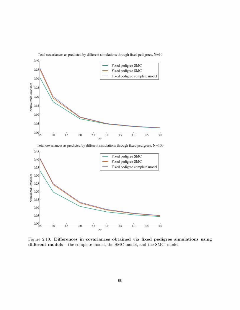
Figure 2.10: Differences in covariances obtained via fixed pedigree simulations usingdifferent models – the complete model, the SMC model, and the SMC’ model.

60

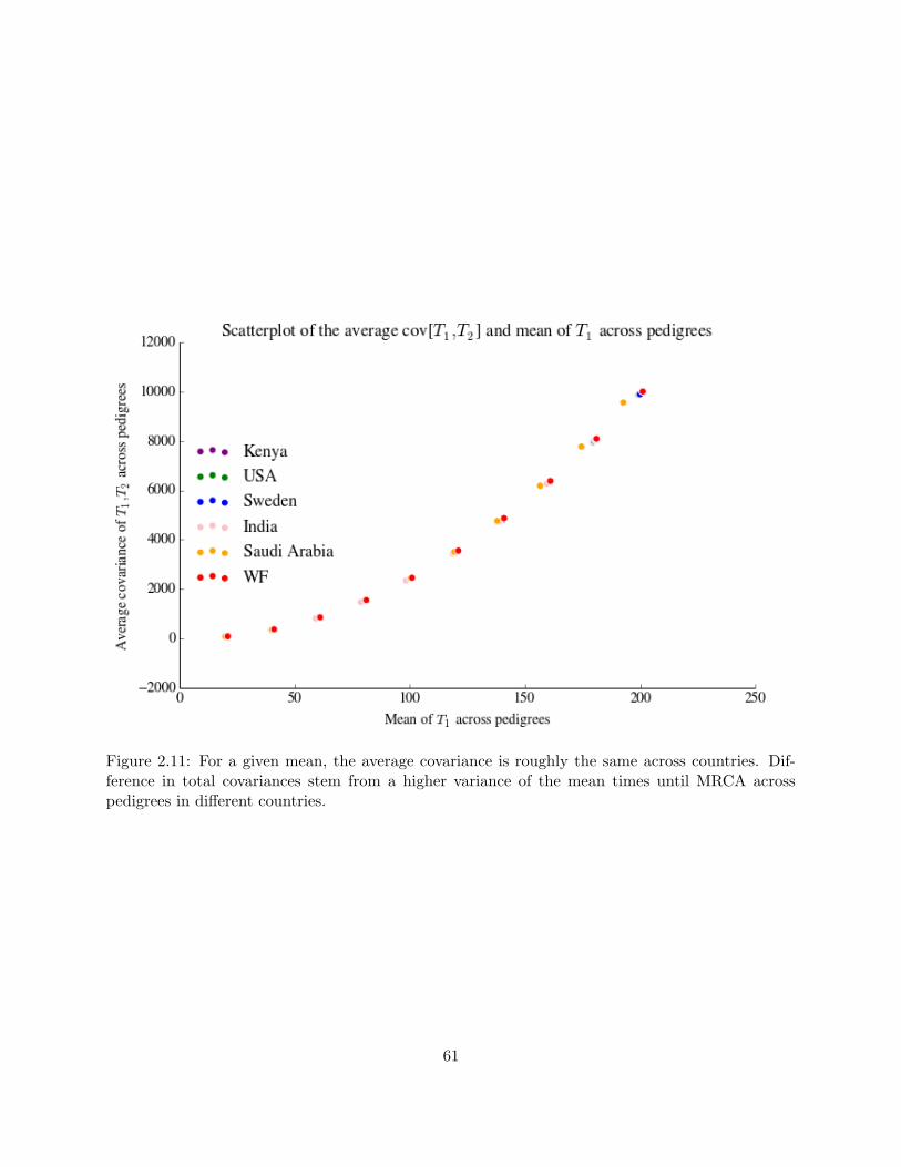
Figure 2.11: For a given mean, the average covariance is roughly the same across countries. Dif-ference in total covariances stem from a higher variance of the mean times until MRCA acrosspedigrees in different countries.

61

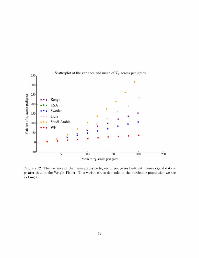
Figure 2.12: The variance of the mean across pedigrees in pedigrees built with genealogical data isgreater than in the Wright-Fisher. This variance also depends on the particular population we arelooking at.

62

Bibliography

A. Bhaskar, A. G. Clark, and Y. S. Song. Distortion of genealogical properties when the sample is

very large. Proc. Natl. Acad. Sci. U. S. A., 111:2385–2390, 2014.

A. H. Bittles and M. L. Black. Global patterns and tables of consanguinity, 2015. URL

“http://consang.net.

J. T. Chang. Recent common ancestors of all present-day individuals. Adv. Appl. Probab., 31:

1002–1026, 1999.

B. Derrida, S. C. Manrubia, and D. H. Zanette. On the genealogy of a population of biparental

individuals. J. Theor. Biol., 203:303–315, 2000.

A. Eriksson, B. Mahjani, and B. Mehlig. Sequential Markov coalescent algorithms for population

models with demographic structure. Theor. Popul. Biol., 76:84–91, 2009.

Y. Erlich. Crowd-sourced genealogy for human genetics, 2015. URL

“http://erlichlab.wi.mit.edu/familinx/.

J. Felsenstein. Accuracy of coalescent likelihood estimates: Do we need more sites, more sequences,

or more loci? Mol. Biol. Evol., 23:691–700, 2006.

R. Griffiths and P. Marjoram. Progress in Population Genetics and Human Evolution, chapter An

ancestral recombination graph, pages 257–270. Springer Verlag, 1997.

J. F. C. Kingman. The coalescent. Stochastic Processes and their Applications,

63

13(3):235–248, 1982. doi: http://dx.doi.org/10.1016/0304-4149(82)90011-4. URL

“http://www.sciencedirect.com/science/article/pii/0304414982900114.

P Marjoram and JD Wall. Fast ”coalescent” simulation. BMC Genetics, 7(1):1–9, 2006. doi:

10.1186/1471-2156-7-16. URL “http://dx.doi.org/10.1186/1471-2156-7-16.

G. A. T. McVean and N. J. Cardin. Approximating the coalescent with recombination. Philos.

Trans. R. Soc. Lond. B Biol. Sci., 360:1387–1393, 2005.

Claudia Moreau, Claude Bherer, Helene Vezina, Michele Jomphe, Damian Labuda,

and Laurent Excoffier. Deep human genealogies reveal a selective advantage to

be on an expanding wave front. Science, 334(6059):1148–1150, 11 2011. URL

“http://science.sciencemag.org/content/334/6059/1148.abstract.

P. L. Ralph. An empirical approach to demographic inference. arXiv:1505.05816, 2015.

N. A. Rosenberg and M. Nordborg. Genealogical trees, coalescent theory, and the analysis of genetic

polymorphisms. Nat. Rev. Genet., 3:380–390, 2002.

K. L. Simonsen and G. A. Churchill. A Markov chain model of coalescence with recombination.

Theor. Popul. Biol., 52:43–59, 1997.

F. Tajima. Evolutionary relationship of dna sequences in finite populations. Genetics, 105:437–460,

1983.

F. Tajima. Statistical method for testing the neutral mutation hypothesis by DNA polymorphism.

Genetics, 123:585–595, 1989.

J. Wakeley, L. King, B. S. Low, and S. Ramachandran. Gene genealogies within a fixed pedigree,

and the robustness of kingman’s coalescent. Genetics, 190:1433–1435, 2012.

G. A. Watterson. On the number of segregating sites in genetical models without recombination.

Theor. Popul. Biol., 7:256–276, 1975.

P. R. Wilton, S. Carmi, and A. Hobolth. The SMC’ is a highly accurate approximation to the

Ancestral Recombination Graph. Genetics, 200:343–355, 2015.

64

C. Wiuf and J. Hein. Recombination as a point process along sequences. Theor. Popul. Biol., 55:

248–259, 1999.

65

Chapter 3

Y chromosome causing differences in

chromatin protein binding profiles

between Y introgression lines of

Drosophila melanogaster

Leandra King, Lene Martinsen, Arvind Sundaram, Tim Sackton, Dan Hartl

(Lene Martinsen, Tim Sackton, and Arvind Sundaram were completely responsible for the experi-

mental design, and for generating the DamID and gene expression data).

3.1 Introduction

Bridges (1916) showed that Drosophila XO males differ from XY males only in that they are sterile,

implying that the Y chromosome plays a role in male fertility but is otherwise mostly devoid of

functional variation. Indeed, the Y chromosome is genetically degenerate, mainly consisting of

large blocks of repetitive DNA with fewer than 20 functional genes (Bachtrog, 2013). Despite this,

there are multiple lines of evidence that suggest a larger role for the Drosophila Y chromosome in

determining phenotype and fitness. The Y chromosome has epigenetic effects on the expression

66

of hundreds of X-linked and autosomal genes (Lemos et al., 2008, 2010). Genes regulated by

the Y chromosome (YRV genes) include certain genes for adaptive traits. For example, it has

been suggested that the extremely low level of polymorphism in the African D. melanogaster Y

chromosome is a result of recent selective sweeps, possibly of Y factors that regulate gene expression

elsewhere in the genome (Larracuente and Clark, 2013). These selective sweeps could be the

result of thermal adaptations: David et al. (2005) found that the Y chromosome was responsible

for 50% of the difference in male heat-induced sterility observed between natural populations in

different climactic environments. They could also be the result of differences in wing musculature,

or fatty acid metabolism, the genes for which are differentially expressed in African versus European

populations (Hutter et al., 2008). Y-linked regulatory variation can then lead to Y-linked regulatory

divergence: introgression of D. sechellia or D. simulans Y chromosomes into a common laboratory

D. simulans background affects male reproductive phenotype (Sackton et al., 2011).

A possible mechanism for the influence of the Y chromosome on global gene expression is via

modulating chromatin state. This mechanism was suggested based on a number of different lines

of evidence. First, it is known that the Y chromosome plays a role in position effect variegation, a

process associated with differences in chromatin conformation (Dimitri and Pisano, 1989). Second,

YRV genes are predominantly in repressive chromatin contexts, which implies that these contexts

must play a role in allowing for the modulation of gene expression by the Y chromosome (Sackton

and Hartl, 2013). Finally, Lemos et al. (2010) showed that XXY females that are genetically

identical except for the Y chromosome have substantially different patterns of expression across the

genome. As the Y chromosome is not transcribed in females, this implies that it affects patterns

of expression by modifying the chromatin landscape. Lemos et al. (2010) suggested a possible

mechanism for this modification: the Y chromosome might play the role of a sink for DNA-binding

proteins, affecting the distribution of chromatin regulators across the genome. Indeed, satellite

repeats, also the binding sites of these regulators, are very variable on the Y chromosome.

A series of spatial arguments further substantiate the hypothesis that the Y chromosome is able

to affect the organization of the genome into chromatin compartments. YRV genes are more likely to

be close to each other in the nucleus than non-YRV genes (Sackton and Hartl, 2013), implying that

67

they might share common regulatory proteins (Naumova and Dekker, 2010). YRV genes also tend

to be associated with the nuclear lamina (Sackton and Hartl, 2013), which is involved in chromatin

organization (Gruenbaum et al., 2003). This yields another hypothesis as to the mechanism by

which the Y chromosome might influence chromatin state across the genome: it might simply be

affecting the spatial configuration of the chromosomes in the nucleus (Sackton and Hartl, 2013).

In this study, we explore whether binding of the D1 and Lamin (LAM) proteins is influenced

by the Y chromosome. We chose these two proteins as they are abundant in areas where the

Y chromosome predominantly exerts its influence: both D1 and LAM mark repressive chromatin

contexts (Filion et al., 2010), and LAM is an important component of the nuclear lamina. In

other words, we expect these proteins to interact with YRV genes. The D1 protein is an AT hook

bearing protein which binds both euchromatic and heterochromatic satellite repeats. The functions

of the D1 protein are not entirely clear: the available research shows conflicting results when it

comes to the necessity of this protein for development (Aulner et al., 2002; Weiler and Chatterjee,

2009). Based on its similarity with mammalian HMGA proteins, D1 might regulate chromatin

structure and the activity of many genes (Reeves and Beckerbauer, 2001). Many transcription

start sites have AT-rich stretches and D1 might therefore play a role in gene regulation by binding

to these sites. Aulner et al. (2002) also suggested that heterochromatic AT-rich regions might serve

as storage sites for D1 proteins with the consequence of affecting the distribution of the protein

elsewhere in the genome. LAM is an intermediate filament protein and an important component

of the nuclear lamina. Located near the inner nuclear membrane and the peripheral chromatin,

the nuclear lamina is an extensive protein network that contributes to nuclear structure. Mutated

or lost nuclear lamina genes cause a wide range of phenotypes, which indicates that they possess

regulatory functions (Gruenbaum et al., 2003).

We screened two African and two European Y introgression lines for variation in chromatin

protein binding using DamID in transgenic flies. DamID is a method for large-scale mapping

of in vivo protein-genome interactions (Greil et al., 2006). The DamID method makes use of

the Escherichia coli protein DNA adenine methyltransferase (DAM), which can be fused to a

protein of interest, in this case LAM or D1. When LAM or D1 bind to DNA, the adenines

68

in DNA surrounding these binding sites are methylated by the DAM protein. Next, adenine-

methylated DNA fragments can be isolated, sequenced, and aligned to the Drosophila melanogaster

reference genome to characterize the pattern of binding. These methylated fragments are indicative

of binding, because methylation of adenine occurs naturally only at very low levels in Drosophila

(Capuano et al., 2014).

We are interested in differences in the binding of the chromatin-related proteins LAM and

D1 between the different Y introgression lines, and whether these are correlated with differences

in gene expression. More generally, we are interested in knowing whether variation within and

between population in Y chromosome sequence could be a non-trivial determinant of epigenetic

state.

3.2 Materials and Methods

3.2.1 Fly lines, fly husbandry and crossing schemes

Y introgression/substitution lines were established from four geographically distinct Drosophila

melanogaster populations: two French (Fr188 and Fr89) and two Zambian (Zi238 and Zi2557)

(Lemos et al., 2008, 2010). Wild-type males from France and Zambia were crossed with females of

the BL4361 fly strain from the Bloomington Drosophila Stock Center and then backcrossed for X

generations to obtain different Y chromosomes introgressed into a common isogenic background.

The 4361 stock is expected to contain very little genetic variation, and in addition upon receipt

was subjected to four additional generations of brother-sister mating to reinforce homozygosity of

the genomic background. The 4361 stock inhabits four recessive markers that are used to select

the flies with the correct genomic background after backcrossing. These markers are yellow (y1; X

chromosome), brown (bw1; chromosome 2), ebony (e1; chromosome 3), and cubitus interruptus and

eyeless (ci1, ey1; chromosome 4). All crosses for each Y-chromosome substitution were carried out

with 15-20 vials with multiple parents per vial; This resulted in several Y-chromosome substituted

males (>30) per line which were subsequently pooled together to give rise to a stable Y-chromosome

substitution line.

69

Flies were kept at 24h light-, temperature-, and humidity-controlled incubators on standard

cornmeal medium. For gene expression analyses, newly emerged flies were collected and aged for

3 days at 25◦C, after which testes were dissected out and both carcass and testes samples were

flash-frozen in liquid nitrogen and stored at -80◦C.

Fly dissections to isolate the testes from the rest of the body (carcass) were done under mi-

croscope in 1xPBS buffer after the flies were anaesthetized using CO2. Ten flies were dissected

and pooled for each sample. We aimed at three biological replicates per sample for both the gene

expression data (RNA-seq) and the protein binding data (DamID-seq). For the DamID-seq we also

used whole flies that were not dissected.

In order to combine the Y chromosome of interest with the DamID fusion constructs, we set up

the following crossing scheme between the Y introgression lines and the DamID transgenic lines:

1. DamID transgenic homozygous virgin females were crossed with males of the Y introgression

lines.

2. F1 males (now heterozygous for the DamID fusion construct) were back-crossed to DamID

transgenic homozygous virgin females in order to obtain flies that had the Y chromosome of

interest and were homozygous for the DamID fusion construct.

3. F2 males were again back-crossed to DamID transgenic homozygous virgin females, but this

time in single fly crosses (1 male + 1 female). This was done in order to screen for male flies

that were homozygous for the DamID fusion construct, i.e. they would lack the markers on

the 3rd and the 4th chromosome that originated from the Y introgression lines (ebony and

eyeless, respectively).

4. The males with the correct genotypes were used to establish stable DamID x Yintrogression

lines for subsequent DamID-seq and RNA-seq analyses.

The DamID transgenic lines containing the LAM and Dam-only constructs provided by the

van Stenseel Lab were homozygous for the DamID construct. The D1 DamID transgenic line from

BestGene was heterozygous for the DamID construct so we performed a crossing scheme with a

70

balancer stock (Bloomington Center stock 9493) to make this line also homozygous before crossing

with the Y introgression lines.

3.2.2 Generation of transgenic lines

The phiC31 unidirectional site-specific recombination method was used to make transgenic flies

containing the protein of interest–D1 and LAM–fused with a DNA adenine methylase (DAM) from

E. coli. An additional transgenic line containing only the DAM protein (DAM-only) was used as

a control. All three lines were produced by Best Gene Inc.; LAM and DAM-only transgenic stocks

provided by the van Steensel Lab at the Netherlands Cancer Institute, while the D1 transgenic stock

was provided by the Hartl Lab at Harvard University. The BDSC strain #24482 of the FlyC31

system, with insertion site 51C on chromosome 2, was used for the transgenesis. In short, the gene of

interest was amplified with primers that have restriction enzyme cut sites. The plasmid vector and

the cDNA gene fragment were then digested with two restriction enzymes, and the gene fragment

was subsequently ligated into the plasmid with T4 DNA ligase. One Shot chemically competent E.

coli cells were transformed with the fusion plasmid and plated onto agar plates containing ampicillin

for selection of clones. The next day bacterial clones were tested with PCR to check that the protein

of interest had ligated into the vector. The clones that gave positive PCR results were chosen and

plasmids were isolated with Plasmid DNA Purification Kit (Qiagen). The isolated plasmids were

sent to Best Gene Inc. for transgenesis into BDSC lines #24482 embryos. The plasmid vectors–

p-attB-NDam[4-HT-intein@L127C]Myc for the transgenesis with the LAM and D1 proteins, and

p-attB-Dam[4-HT-intein@L127C]Myc[closed] for the DAM-only controls-were constructed by the

van Stenseel Lab (Filion et al., 2010; van Bemmel et al., 2010). These DamID transgenic lines were

then crossed with the Y introgression lines.

3.2.3 DamID

DamID was performed on the testes, the carcass, and the whole fly as in Vogel et al. (2007) with

minor adjustments. In brief, genomic DNA was isolated from the DamIDxY lines by using the

DNeasy Blood and Tissue Kit (Qiagen). To obtain the methylated fragments, genomic DNA was

71

then digested with the restriction enzyme DpnI which cleaves only Gm6ATC sites, not unmethy-

lated sites. Then a double-stranded adaptor oligonucleotide was ligated to the cleaved DNA ends.

Following ligation, the DNA is treated with the restriction enzyme DpnII which cuts only unmethy-

lated GATC sites. The sequential use of DpnI and DpnII creates a double selection for methylated

DNA fragments: only methylated GATC sequences are cut by DpnI and therefore ligated to the

adaptors, and only fragments in which all GATCs are methylated are resistant to degradation by

DpnII and can therefore be amplified. The methylated fragments are then amplified by PCR using

primers that are complementary to the adaptor sequence. After amplification the fragments are

analyzed on an agarose gel. A smear of genomic methylated fragments will be visible on the gel, in

addition to bands from amplified methylated plasmid DNA. The PCR products were purified with

QIAquick PCR Purification Kit (Qiagen) and used for next-generation sequencing.

3.2.4 DamID and Next-Generation Sequencing

The DNA content of the PCR products was measured with Qubit and 200ng (when available) was

used as input for the Illumina Next Generation Sequencing protocol using the TruSeq Nano DNA

Library Prep Kit. The DNA content of the testis samples was sometimes lower than 200 ng due

to limitation of available tissue. The samples were transferred to crimp-cap MicroTube ASA vials

for shearing of the DNA in Covaris. The settings used were duty cycle = 10%, intensity = 5,

cycles/burst = 200, time = 45 sec as recommended by the Illumina Nano Kit.

3.2.5 Gene expression

Total RNA was extracted with TRIzol (Invitrogen) from carcass and testes tissues and treated with

DNaseI according to standard protocols. RNA extractions were kept at -80◦C. RNA-seq libraries

were prepared using the Illumina TruSeq RNA Library Prep Kit v2 according to the manufacturer’s

protocol. The samples were sequenced on an Illumina HighSeq 2000/2500 machine.

72

3.2.6 Bioinformatic analysis

Data availability

DamID sequences and expression data will be deposited in NCBI’s Gene Expression Omnibus.

Data preprocessing

Raw reads from DamID sequencing were processed using Trimmomatic v0.33 to remove sequencing

(Illumina) adapters and trim low quality reads. Cleaned data for each sample was further separated

into four bins based on the presence of AdRp, AdRt, AdRb adapters or presence of none of these.

Double-stranded adaptor oligonucleotides that were used to extract DamIDs were trimmed off

using cutadapt v1.4.1 and the reads were aligned to the Fly genome (Dmel r6.07) using bowtie2.

Based on the alignment statistics, reads from AdRt and AdRb bins were not analyzed after this

step. Aligned data was converted to bed format using bedtools and extended by (225/212 nts) the

average length of the fragments used for preparing the library for sequencing. Location of GATC

regions in the fly genome were identified using HOMER v4.7.2 and the reads aligning to these

regions in each of the above processed samples were counted using bedtools coverage tool.

Gene expression and Protein binding

Our first aim was to find differentially expressed genes across Y introgression lines. To this

end, using our RNA-seq data from testes and carcass tissues, we quantified abundances of non-

mitochondrial transcripts using the program kallisto (Bray et al., 2016). The first step was to make

a transcriptome index using the flybase Drosophila melanogaster r6.07 transcriptome file. We used

the following parameters for each strain: the average fragment length for that strain, 30 as an

estimate of the standard deviation for each strain, and 100 bootstrap samples. At the end of this

step, we discarded strains with too many undetected transcripts.

We used the library DESeq2 in R (Love et al., 2014) for the analysis of differential expression.

This differential expression/binding analysis models the read counts Kij for each gene i and sample

j as following a negative binomial distribution:

73

Kij = NB(sjqij , αi)

where sj is a sample-specific normalization factor, qij is proportional to the concentration of cDNA

fragments from the gene in the sample, and αi is a dispersion factor which models variability within

replicates.

We also use the DESeq2 library in R to analyze differential protein binding.

All code used for the analysis is available at: https://github.com/tsackton/YRV-damID.

3.3 Results

3.3.1 Gene expression

We are interested in identifying differentially expressed genes across Y introgression lines. This will

enable us to replicate results from previous studies (Sackton and Hartl, 2013), determine whether

or not variation is structured by country, and later correlate patterns of differential expression with

patterns of differential binding.

We find that the biggest differences in gene expression are due to tissue type (carcass vs testes).

When studying combined carcass and testes data, we identify 2574 statistically significantly dif-

ferentially expressed genes at the 5% significance level, which is greater than 4 times the number

of differentially expressed genes found by running the analysis separately for carcass and testes.

As a result, we conservatively choose to study carcass and testes data separately. Conditioning

on carcass data, we find 463 statistically significantly differentially expressed genes based on Y

line. Analysis of testes data does not show the same level of differential expression, with only 150

statistically significant genes. 15 percent of the carcass data is low count data, relative to only 7.7

percent of the testes data, which implies that the lower number of differentially expressed genes in

testes is not due to the testes data being of lower quality. A Fisher’s exact test reveals that there

is significant overlap between the differentially expressed genes found in our experiment in both

carcass and testes data, and those described in Sackton and Hartl (2013) (p-value< .001).

To test whether Y-linked regulatory variation primarily represents inter-population divergence,

74

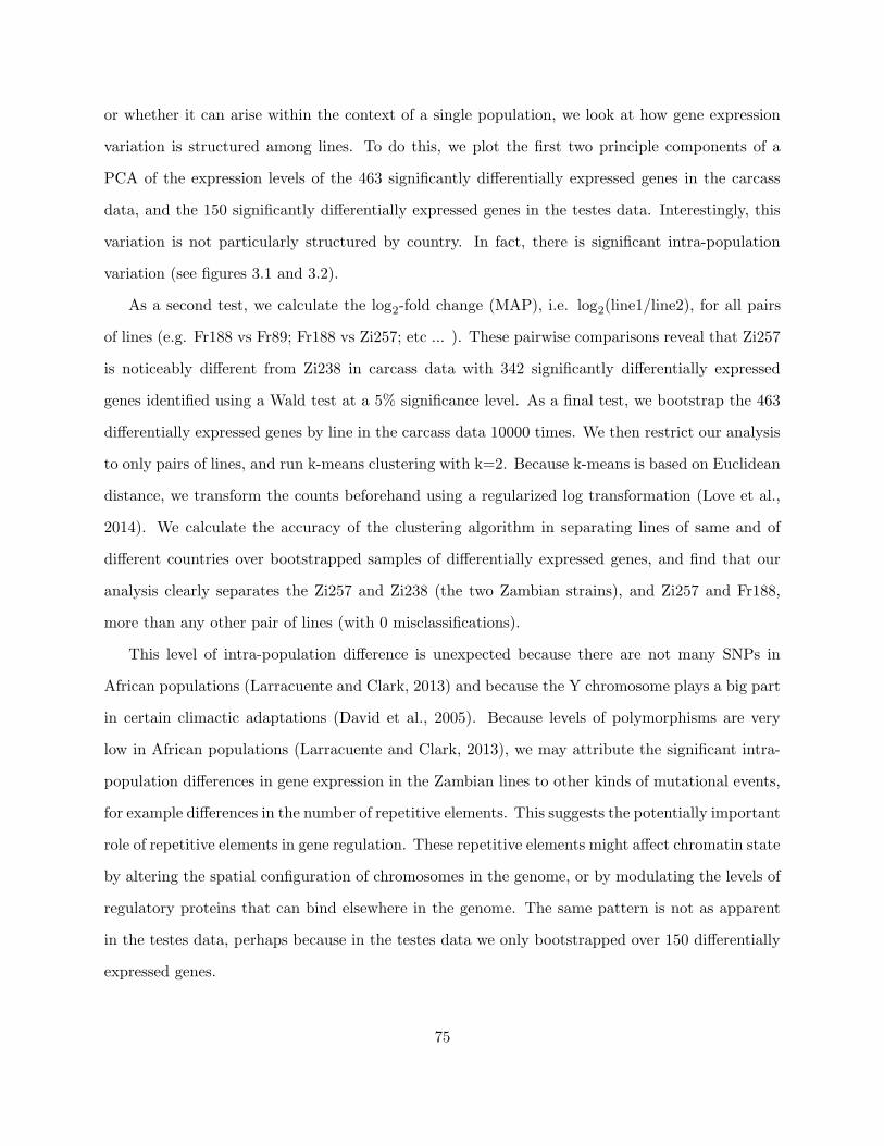
or whether it can arise within the context of a single population, we look at how gene expression

variation is structured among lines. To do this, we plot the first two principle components of a

PCA of the expression levels of the 463 significantly differentially expressed genes in the carcass

data, and the 150 significantly differentially expressed genes in the testes data. Interestingly, this

variation is not particularly structured by country. In fact, there is significant intra-population

variation (see figures 3.1 and 3.2).

As a second test, we calculate the log2-fold change (MAP), i.e. log2(line1/line2), for all pairs

of lines (e.g. Fr188 vs Fr89; Fr188 vs Zi257; etc ... ). These pairwise comparisons reveal that Zi257

is noticeably different from Zi238 in carcass data with 342 significantly differentially expressed

genes identified using a Wald test at a 5% significance level. As a final test, we bootstrap the 463

differentially expressed genes by line in the carcass data 10000 times. We then restrict our analysis

to only pairs of lines, and run k-means clustering with k=2. Because k-means is based on Euclidean

distance, we transform the counts beforehand using a regularized log transformation (Love et al.,

2014). We calculate the accuracy of the clustering algorithm in separating lines of same and of

different countries over bootstrapped samples of differentially expressed genes, and find that our

analysis clearly separates the Zi257 and Zi238 (the two Zambian strains), and Zi257 and Fr188,

more than any other pair of lines (with 0 misclassifications).

This level of intra-population difference is unexpected because there are not many SNPs in

African populations (Larracuente and Clark, 2013) and because the Y chromosome plays a big part

in certain climactic adaptations (David et al., 2005). Because levels of polymorphisms are very

low in African populations (Larracuente and Clark, 2013), we may attribute the significant intra-

population differences in gene expression in the Zambian lines to other kinds of mutational events,

for example differences in the number of repetitive elements. This suggests the potentially important

role of repetitive elements in gene regulation. These repetitive elements might affect chromatin state

by altering the spatial configuration of chromosomes in the genome, or by modulating the levels of

regulatory proteins that can bind elsewhere in the genome. The same pattern is not as apparent

in the testes data, perhaps because in the testes data we only bootstrapped over 150 differentially

expressed genes.

75

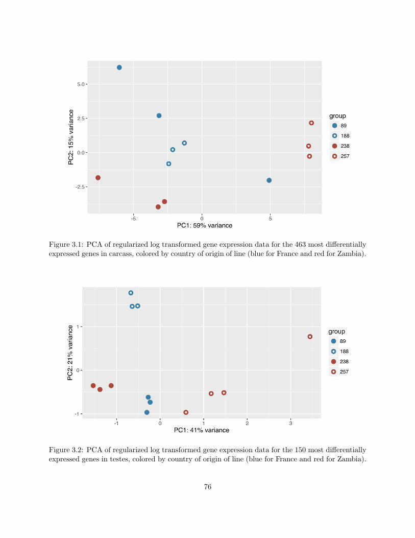
Figure 3.1: PCA of regularized log transformed gene expression data for the 463 most differentiallyexpressed genes in carcass, colored by country of origin of line (blue for France and red for Zambia).

Figure 3.2: PCA of regularized log transformed gene expression data for the 150 most differentiallyexpressed genes in testes, colored by country of origin of line (blue for France and red for Zambia).

76

Carcass Testes Whole fly

D1 7222 (5.06%) 336 (0.086%) 40179 (14.10%)LAM 140514 (40%) 118484 (36.14%) 182332 (47.91%)

Table 3.1: Binding Results. We report the number of methylated GATC sites at the 0.1%significance level for each tissue-protein combination. As the number of low-counts is variable, inparentheses we express the number of significant sites as a percentage of non-low count data.

3.3.2 Protein binding

It is clear that the Y chromosome affects gene expression, and it is hypothesized that it does so by

modifying the distribution of the genome into different chromatin compartments. Using the DamID

technique, we are interested in identifying regions of the genome that are differentially bound by

D1 and LAM depending on the Y introgression line. We expect both of these proteins to interact

with YRV genes.

To identify regions of the genome bound by either LAM or D1, we compared sequencing reads

from the LAM or D1 lines to a control with just the DAM protein (not fused to a target protein),

and identified bound regions based on a significant likelihood ratio test (LRT) for protein in DESeq2

(full model: ∼Protein + Line; reduced model: ∼Line). This test reveals that a variable portion of

the genome (table 3.1) is bound by each protein across tissue types (testes, carcass, whole fly). We

identify between 336 (for testes D1, our lowest quality sample) and 182332 variable sites across the

genome, depending on tissue and protein. Binding is much higher for LAM than D1.

We are primarily interested in regions of the genome where binding of either LAM or D1 varies

depending on the Y chromosome carried by the transgenic line. To identify these regions, we

use another LRT in DESeq2, but now we hope to detect a significant line by protein interaction,

meaning that the effect of D1 or LAM vs DAM-only varies among lines (full model: ∼Protein +

Line + Protein:Line; reduced model: ∼Protein + Line). In carcass, testes, and whole-fly tissues,

we are able to identify regions of differential binding using a LRT test (see table 3.2). LAM binding

is in general positively correlated across tissue types. In particular line by tissue subsets, LAM

binding is negatively correlated to D1 binding (see figure 3.3). This holds even conditioning on

heterochromatin state being ‘BLACK’, one of the repressive heterochromatin states described by

Filion et al. (2010).

77

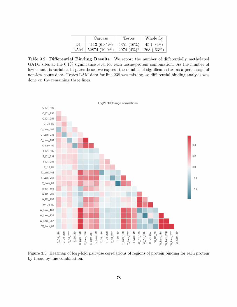
Carcass Testes Whole fly

D1 4113 (6.35%) 4351 (16%) 45 (.04%)LAM 52874 (19.9%) 2974 (4%)* 268 (.63%)

Table 3.2: Differential Binding Results. We report the number of differentially methylatedGATC sites at the 0.1% significance level for each tissue-protein combination. As the number oflow-counts is variable, in parentheses we express the number of significant sites as a percentage ofnon-low count data. Testes LAM data for line 238 was missing, so differential binding analysis wasdone on the remaining three lines.

Figure 3.3: Heatmap of log2-fold pairwise correlations of regions of protein binding for each proteinby tissue by line combination.

78

It is important to note some aspect of these data which could affect our results. Both our

pre- and post- sequencing results suggest that D1 testes samples are of notably low quality, so we

expect not to be able to draw many conclusions from this data. Also, the number of differentially

expressed lines in whole fly is low in comparison to testes and carcass, especially in the case of

LAM binding. As differential binding is positively correlated for the same protein in carcass and

testes data, we do not expect lower counts in whole fly data.

We identify differentially bound regions by looking for stretches of more than 25 contiguous

significant p-values, using a 5% significance level. We look for contiguous p-values because we

expect binding to extend over multiple GATC sites. According to this criterion, one of the most

differentially bound loci is the Stellate locus (Ste) on the X chromosome, which is differentially

bound by LAM in whole fly data. Negative regulatory interaction exists between this locus and

the Suppressor of Stellate Su(Ste) locus on the Y chromosome. More precisely, the silencing of

the Ste locus is mediated by dsRNA (Aravin et al., 2001). It has been hypothesized that the Ste

-Su(Ste) system is dispensable, and evolved as a self-maintaining parasitic system (Bozzetti et al.,

1995). We do not find Ste to be significantly differentially expressed in different Y introgression

lines. However, it is difficult to determine statistical significance for this gene because expression

levels are (as expected) very low.

Another region of clear differential binding is the 5S rRNA locus on chromosome 2R, which is

differentially bound both by LAM in testes and by D1 in carcass data (see figure 3.4). Interestingly,

the sign of the log2-fold change of D1 in carcass data and LAM in testes data at this locus is not

consistent across lines. 5S rRNA acts in collaboration with rRNA products derived from blocks

located on the X and Y chromosomes to form the ribosome. Therefore, we would expect there

to be correlation in the expression levels of all of these rRNAs. The rRNA genes in the 45S

block of Drosophila melanogaster are particularly AT-rich (Tautz et al., 1988), so we might expect

involvement of D1. Interestingly, previous research has shown that rDNA contributes to global

chromatin regulation (Paredes and Maggert, 2009), and that variation in copy number affects

genome-wide expression patterns (Paredes et al., 2011).

Both of the Ste locus and the 5S rRNA locus consist of Y-related tandem repeats, which suggests

79

Figure 3.4: log2-fold change values of the binding of LAM and D1 versus DAM at the 5S rRNAlocus. In green is the region of more than 25 contiguous significant p-values at the 5% significancelevel.

that some of the observed differential binding could potentially be driven by variation in Y-linked

transcription of non-coding RNAs. However, this is not the only role of the Y chromosome: we

also found a stretch of DNA of about 100 kbp located near the centromere on chromosome 2 to be

differentially bound by LAM in whole fly data (2L:22409449..22508017). The presence of this long

differentially bound stretch of DNA allows us to conclude that multiple different kinds of genomic

regions are influenced by the Y chromosome, not just tandem repeats.

The heterochromatic sink model

There are many mechanisms by which the Y chromosome might be able to affect chromatin state

across the genome. One proposed model is the heterochromatic sink model (Lemos et al., 2010),

which suggests that the Y chromosome acts as a protein sink, influencing the quantity of protein

available to bind at other sites in the genome. In its simplest form, this model yields a very clear

prediction: we would expect some strains to show significantly lower levels of binding than other

strains. In fact, an ANOVA F-test rejects the hypothesis that the mean log2-fold change of D1

binding in comparison to DAM is the same across all strains (p-value < .001). These means are

80

0.6 in line 188, .22 in line 89, .09 in line 257, and .13 in line 238 (they are all positive because we

expect D1 to bind on average more than DAM). This allows us to conclude that there are large

scale differences in binding among the four lines, which is consistent with the heterochromatic sink

model, while not providing definitive evidence for it. However, the results of the F-test are at least

suggestive that there might be some global or higher order models.

3.4 Discussion

It is known that the Y chromosome is able to influence gene expression throughout the genome.

In this study, we have provided more evidence for Y induced differential expression, and the YRV

genes we identified overlap significantly with those previously discovered. We found that variation

in gene expression is not particularly structured by country, which given the expected differences

between countries based on Y-associated adaptations (such as thermal adaptations), implies that

intra-population variation is high and overlaps with inter-population variation. Also, because there

are very few SNP differences in African strains, these results argue that variation in repetitive

regions on the Y chromosome likely play an important role in modulating transcriptional activity

across the whole genome.

Differential binding does occur, most notably in regions of tandem repeats, and in centromeric

regions. This implies that the Y chromosome probably affects chromatin binding across the genome

in a variety of different ways, and that in some cases it is very likely that RNA plays a mediating

role. Significant differences in mean binding of D1 across Y introgression lines points to global

models, like the heterochromatic sink model.

Future work will involve correlating regions of differential expression with regions of differential

binding to provide further insight into the mechanism by which the Y chromosome affects expression

on the X chromosome and the autosomes.

81

Bibliography

Alexei A. Aravin, Natalia M. Naumova, Alexei V. Tulin, Vasilii V. Vagin, Yakov M. Rozovsky,

and Vladimir A. Gvozdev. Double-stranded rna-mediated silencing of genomic tandem repeats

and transposable elements in the d. melanogaster germline. Current Biology, 11(13):1017–1027,

7 2001. doi: http://dx.doi.org/10.1016/S0960-9822(01)00299-8.

Nathalie Aulner, Caroline Monod, Guillaume Mandicourt, Denis Jullien, Olivier Cuvier, Alhoussey-

nou Sall, Sam Janssen, Ulrich K Laemmli, and Emmanuel Kas. The at-hook protein d1 is essential

for drosophila melanogaster development and is implicated in position-effect variegation. Molec-

ular and Cellular Biology, 22(4):1218–1232, 02 2002. doi: 10.1128/MCB.22.4.1218-1232.2002.

Doris Bachtrog. Y-chromosome evolution: emerging insights into processes of y-chromosome de-

generation. Nat Rev Genet, 14(2):113–124, 02 2013.

M P Bozzetti, S Massari, P Finelli, F Meggio, L A Pinna, B Boldyreff, O G Issinger, G Palumbo,

C Ciriaco, and S Bonaccorsi. The ste locus, a component of the parasitic cry-ste system of

drosophila melanogaster, encodes a protein that forms crystals in primary spermatocytes and

mimics properties of the beta subunit of casein kinase 2. Proceedings of the National Academy

of Sciences of the United States of America, 92(13):6067–6071, 06 1995.

Nicolas L Bray, Harold Pimentel, Pall Melsted, and Lior Pachter. Near-optimal probabilistic rna-seq

quantification. Nat Biotech, 34(5):525–527, 05 2016.

Calvin B Bridges. Non-disjunction as proof of the chromosome theory of heredity. Genetics, 1(1):

1–52, 01 1916.

82

Floriana Capuano, Michael Mulleder, Robert Kok, Henk J Blom, and Markus Ralser. Cytosine

dna methylation is found in drosophila melanogaster but absent in saccharomyces cerevisiae,

schizosaccharomyces pombe, and other yeast species. Analytical Chemistry, 86(8):3697–3702, 04

2014. doi: 10.1021/ac500447w.

JR David, LO Araripe, M Chakir, H Legout, B Lemos, G Petavy, C Rohmer, D Joly, and

B Moreteau. Male sterility at extreme temperatures: a significant but neglected phenomenon for

understanding drosophila climatic adaptations. Journal of Evolutionary Biology, 18(4):838–846,

2005. doi: 10.1111/j.1420-9101.2005.00914.x.

P Dimitri and C Pisano. Position effect variegation in drosophila melanogaster: Relationship

between suppression effect and the amount of y chromosome. Genetics, 122(4):793–800, 08 1989.

Guillaume J Filion, Joke G van Bemmel, Ulrich Braunschweig, Wendy Talhout, Jop Kind, Lu-

cas D Ward, Wim Brugman, Ines de Castro Genebra de Jesus, Ron M Kerkhoven, Harmen J

Bussemaker, and Bas van Steensel. Systematic protein location mapping reveals five principal

chromatin types in drosophila cells. Cell, 143(2):212–224, 10 2010. doi: 10.1016/j.cell.2010.09.009.

Frauke Greil, Celine Moorman, and Bas and van Steensel. DamID: Mapping of In Vivo Protein–

Genome Interactions Using Tethered DNA Adenine Methyltransferase, volume Volume 410, pages

342–359. Academic Press, 2006. ISBN 0076-6879. doi: http://dx.doi.org/10.1016/S0076-6879(06)

10016-6.

Yosef Gruenbaum, Robert D Goldman, Ronit Meyuhas, Erez Mills, Ayelet Margalit, Alexandra

Fridkin, Yaron Dayani, Miron Prokocimer, and Avital and Enosh. The Nuclear Lamina and

Its Functions in the Nucleus, volume Volume 226, pages 1–62. Academic Press, 2003. ISBN

0074-7696. doi: http://dx.doi.org/10.1016/S0074-7696(03)01001-5.

Stephan Hutter, Sarah S Saminadin-Peter, Wolfgang Stephan, and John Parsch. Gene expression

variation in african and european populations of drosophila melanogaster. Genome Biology, 9

(1):R12–R12, 2008. doi: 10.1186/gb-2008-9-1-r12.

83

A. M. Larracuente and A. G. Clark. Surprising differences in the variability of y chromosomes

in african and cosmopolitan populations of drosophila melanogaster. Genetics, 193(1):201–214,

2013.

Bernardo Lemos, Luciana O. Araripe, and Daniel L. Hartl. Polymorphic y chromosomes harbor

cryptic variation with manifold functional consequences. Science, 319(5859):91–93, 01 2008.

Bernardo Lemos, Alan T. Branco, and Daniel L. Hartl. Epigenetic effects of polymorphic y chro-

mosomes modulate chromatin components, immune response, and sexual conflict. Proceedings of

the National Academy of Sciences, 107(36):15826–15831, 09 2010.

MI Love, W Huber, and S Anders. Moderated estimation of fold change and dispersion for rna-seq

data with deseq2. Genome Biology, 15:550, 2014.

Natalia Naumova and Job Dekker. Integrating one-dimensional and three-dimensional maps of

genomes. Journal of Cell Science, 123(12):1979–1988, 06 2010. doi: 10.1242/jcs.051631.

Silvana Paredes and Keith A. Maggert. Ribosomal dna contributes to global chromatin regulation.

Proceedings of the National Academy of Sciences, 106(42):17829–17834, 10 2009.

Silvana Paredes, Alan T Branco, Daniel L Hartl, Keith A Maggert, and Bernardo Lemos. Ribo-

somal dna deletions modulate genome-wide gene expression: “rdna–sensitive”genes and natural

variation. PLoS Genetics, 7(4):e1001376, 04 2011. doi: 10.1371/journal.pgen.1001376.

Raymond Reeves and Lois Beckerbauer. Hmgi/y proteins: flexible regulators of transcription and

chromatin structure. Biochimica et Biophysica Acta (BBA) - Gene Structure and Expression,

1519(1–2):13–29, 5 2001. doi: http://dx.doi.org/10.1016/S0167-4781(01)00215-9.

Timothy B Sackton and Daniel L Hartl. Meta-analysis reveals that genes regulated by the y chro-

mosome in drosophila melanogaster are preferentially localized to repressive chromatin. Genome

Biology and Evolution, 5(1):255–266, 2013. doi: 10.1093/gbe/evt005.

Timothy B Sackton, Horacio Montenegro, Daniel L Hartl, and Bernardo Lemos. Interspecific y

chromosome introgressions disrupt testis-specific gene expression and male reproductive pheno-

84

types in drosophila. Proceedings of the National Academy of Sciences of the United States of

America, 108(41):17046–17051, 10 2011. doi: 10.1073/pnas.1114690108.

D Tautz, J M Hancock, D A Webb, C Tautz, and G A Dover. Complete sequences of the rrna

genes of drosophila melanogaster. Molecular Biology and Evolution, 5(4):366–376, 07 1988.

J. G. van Bemmel, L. Pagie, U. Braunschweig, W. Brugman, W. Meuleman, R. M. Kerkhoven,

and B. van Steensel. The insulator protein su(hw) fine-tunes nuclear lamina interactions of the

drosophila genome. PLoS ONE, 5(11):e15013, 2010.

Maartje J Vogel, Daniel Peric-Hupkes, and Bas van Steensel. Detection of in vivo protein-dna

interactions using damid in mammalian cells. Nat. Protocols, 2(6):1467–1478, 06 2007.

Karen S Weiler and Suman Chatterjee. The multi-at-hook chromosomal protein of drosophila

melanogaster, d1, is dispensable for viability. Genetics, 182(1):145–159, 05 2009. doi: 10.1534/

genetics.109.101386.

85