HAL Id: hal-02380401https://hal.archives-ouvertes.fr/hal-02380401

Submitted on 26 Nov 2019

HAL is a multi-disciplinary open accessarchive for the deposit and dissemination of sci-entific research documents, whether they are pub-lished or not. The documents may come fromteaching and research institutions in France orabroad, or from public or private research centers.

L’archive ouverte pluridisciplinaire HAL, estdestinée au dépôt et à la diffusion de documentsscientifiques de niveau recherche, publiés ou non,émanant des établissements d’enseignement et derecherche français ou étrangers, des laboratoirespublics ou privés.

Estimating the end-of-life of PEM fuel cells: Guidelinesand metrics

Marine Jouin, Mathieu Bressel, Simon Morando, Rafael Gouriveau, DanielHissel, Marie Péra, Noureddine Zerhouni, Samir Jemei, Mickaël Hilairet,

Belkacem Bouamama

To cite this version:Marine Jouin, Mathieu Bressel, Simon Morando, Rafael Gouriveau, Daniel Hissel, et al.. Estimatingthe end-of-life of PEM fuel cells: Guidelines and metrics. Applied Energy, Elsevier, 2016, 177, pp.87- 97. �hal-02380401�

Estimating the end-of-life of PEM fuel cells : guidelines and metrics

Marine Jouin1,2∗, Mathieu Bressel1,2,3 , Simon Morando1,2 , Rafael Gouriveau1,2 , Daniel Hissel1,2 , Marie-Cecile Pera1,2 ,Noureddine Zerhouni1,2 , Samir Jemei1,2 , Mickael Hilairet1,2 , Belkacem Ould Bouamama3

1 FEMTO-ST Institute, UMR CNRS 6174 - UBFC / ENSMM / UTBM / UFC, 24 rue Alain Savary, 25000 Besancon, France2FC-LAB Research, FR CNRS 3539, Rue Thierry Mieg, 90010 Belfort, France

3CRIStAL, UMR CNRS 9189 - Universite de Lille-Sciences et Technologies, Avenue Paul Langevin, 59655 Villeneuve d’Ascq, Francename.lastname@femto-st.fr

Abstract

Prognostics applications on PEMFC are developing these last years. Indeed, taking decision to extend the lifetime ofa PEMFC stack based on behavior and remaining useful life predictions is seen as a promising solution to tackle thetoo short life’s issue of PEMFCs. However, the development of prognostics shows some lacks in the literature. Indeed,performing prognostics requires health indicators that reflect the state of health of stack, while being able to interpretthem in an industrial context. It is also important to propose criteria to set its end of life. Moreover, to trust anyprognostics’ application, one should be able to evaluate the performance of its algorithms with respect to standards.To help launching a discussion on these subjects among scientific and industrial actors, this paper addresses some ofthe issues encountered when performing prognostics of a PEMFC stack. After showing the link between prognosticsand decision, this paper proposes guidelines to set the limits of a prognostics approach. The definitions of healthy anddegraded modes are discussed as well as how to choose the time instant to perform predictions. Then, three criteriabased on the power produced by the stack are proposed as indicators of the state of health of the stack. The definition ofthe end of life of the stack is also discussed before proposing some criteria to assess the performance of any prognosticsalgorithm on a PEMFC. Some perspectives of works are also discussed before concluding.

Keywords: Proton exchange membrane (PEM) fuel cell, Prognostics, Remaining useful life, PHM

1. Introduction1

In the current context of energy transition, re-2

placing fossil energies by alternative power sources3

such as fuel cells appears as a promising solution4

[1, 2]. Fuel cells can be used in a great number of5

applications such as transportation, mobile elec-6

tronic devices, micro-CHP (Combined Heat and7

Power), etc. [3, 4].8

Despite their great industrial potential and large scale-9

projects all around the world, fuel cells experience diffi-10

culty to enter the energy market and this industry remains11

brittle [5]. Actual obstacles are, among others, high ex-12

ploitation cost, public acceptance and life duration that13

remains to short [6]. Indeed, for the fuel cells of interest in14

this paper, namely Proton Exchange Membrane Fuel Cells15

(PEMFC), current lifetimes are around 2000-3000 hours16

when 8000 hours are needed for transportation applica-17

tions and 100 000 hours for stationary. Different options18

are available to tackle the lifetime issue: working on the19

material, reducing the causes of degradation, improving20

the stack design, implementing new supervision and man-21

agement strategies, etc. This last solution appears to be22

∗Corresponding author, Tel.: +33 (0)3 81 40 29 04, Fax +33 (0)381 40 28 09

of great interest and has started to appear in the PEMFC23

field through Prognostics and Health Management (PHM)24

[7, 8].25

PHM is an engineering discipline originated from the pre-26

dictive maintenance. It is defined by [9] as “a maintenance27

and asset management approach utilizing signals, mea-28

surements, models and algorithms to detect, assess and29

track degraded health, and to predict failure progression”.30

In other terms, by continuously monitoring the system, it31

is possible to detect and anticipate, thanks to prognostics,32

the occurrence of failures and to take decisions at the right33

time to preserve the system. These actions enable the sys-34

tem to reach the end of its mission. Prognostics is widely35

accepted as a key stage of PHM. Indeed, based on the sys-36

tem knowledge and historical data, it allows predicting the37

future State of Health (SoH) of the system. Prognostics38

is defined as the “estimation of the operating time before39

failure and the risk of existence or later appearance of one40

or more failure modes” [10]. The operating time before41

failure is more commonly known as the Remaining Useful42

Life (RUL).43

During the last years, prognostics has started to be ap-44

plied to PEMFC. Different types of approaches are pro-45

posed: model-based approaches [11, 12, 13], data-driven46

approaches [14, 15, 16] and a combination of both, hy-47

Preprint submitted to Elsevier May 5, 2016

brid approaches [17]. The growing interest of the scientific48

community to that subject has also been shown thanks49

to the IEEE PHM data challenge 2014 [18] in which dif-50

ferent propositions for SoH predictions [19, 20] and RUL51

estimates [21, 22] were presented.52

Despite those recent works, a deep thinking and53

standards proposal on how to perform prognostics54

on PEMFC are needed. Although different consid-55

erations about prognostics standards are available56

[9, 23], they are too general and further question-57

ing is required for the PEMFC case.58

1. Which level of granularity should be chosen on the59

PEMFC?60

2. How to define the healthy and degraded modes for a61

PEMFC?62

3. When prognostics should be performed?63

4. Which health indicator should be used to perform64

prognostics?65

5. How to define the End-of-Life (EoL) of a PEMFC?66

6. How can the prognostics’ performances be evaluated?67

To the authors’ knowledge none of these questions68

are answered in the literature. Consequently, this69

paper intends to propose solutions and guidance70

to start answering these questions and going to-71

wards standardization. The main contribution is72

to propose general solutions that are completely73

independent of prognostics tools and that can be74

adapted with any approach. New practitioners can75

use these guidelines as tutorial to start performing76

prognostics of PEMFC.77

To adopt a logical reasoning, the paper follows the chrono-78

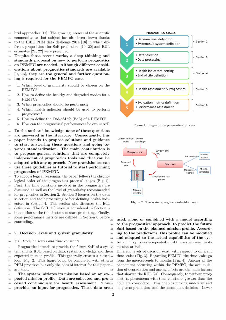
logical order of the prognostics process’ stages (Fig 1).79

First, the time constants involved in the prognostics are80

discussed as well as the level of granularity recommended81

for prognostics in Section 2. Section 3 focuses on the data82

selection and their processing before defining health indi-83

cators in Section 4. This section also discusses the EoL84

definition. The SoH definition is considered in Section 585

in addition to the time instant to start predicting. Finally,86

some performance metrics are defined in Section 6 before87

concluding.88

2. Decision levels and system granularity89

2.1. Decision levels and time constants90

Prognostics intends to provide the future SoH of a sys-91

tem and its RUL based on data, system knowledge and the92

expected mission profile. This generally creates a closed93

loop, Fig. 2. This figure could be completed with other94

PHM processes but only the ones of interest for this paper95

are kept.96

The system initiates its mission based on an ex-97

pected mission profile. Data are collected and pro-98

cessed continuously for health assessment. This99

provides an input for prognostics. These data are100

1•Decision level definition• System/sub‐system definition

2•Data selection•Data processing

3•Health indicators setting• End of Life definition

4•Health assessment & Prognostics

5•Evaluation metrics definition•Performance assessment

PROGNOSTICS’ STAGES

Section 2

Section 3

Section 4

Section 5

Section 6

Figure 1: Stages of the prognostics’ process

Current mission profile

Processed data

System knowledge

Mission completed

Prognostics

Decision

SOH(t  t+h)RUL

Modified mission profile

FC

Objectives reached

Mission initiated

Mission abortedEoL reached

Figure 2: The system-prognostics-decision loop

used, alone or combined with a model according101

to the prognostics’ approach, to predict the future102

SoH based on the planned mission profile. Accord-103

ing to the predictions, this profile can be modified104

and adapted to the actual capabilities of the sys-105

tem. This process is repeated until the system reaches its106

mission or fails.107

Different levels of decision exist with respect to different108

time scales (Fig. 3). Regarding PEMFC, the time scales go109

from the microseconds to months (Fig. 4). Among all the110

phenomena occurring within the PEMFC, the accumula-111

tion of degradation and ageing effects are the main factors112

that shorten the RUL [24]. Consequently, to perform prog-113

nostics, phenomena with time constants greater than the114

hour are considered. This enables making mid-term and115

long term predictions and the consequent decisions. Lower116

2

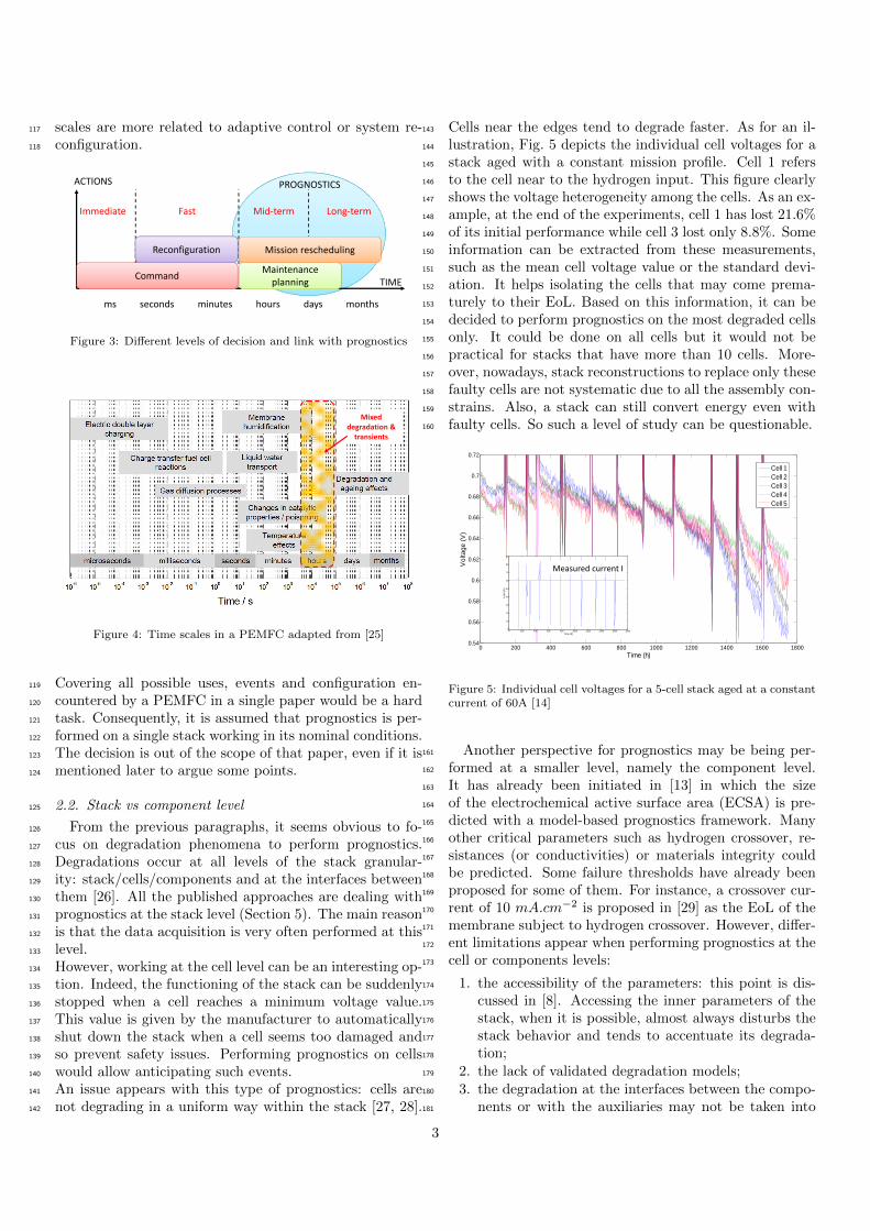
scales are more related to adaptive control or system re-117

configuration.118

ms seconds minutes hours days months

TIME

ACTIONS

Command 

Reconfiguration  

Maintenance planning 

Mission rescheduling

Immediate  Fast  Mid‐term  Long‐term 

PROGNOSTICS

Figure 3: Different levels of decision and link with prognostics

Mixed degradation & transients

Figure 4: Time scales in a PEMFC adapted from [25]

Covering all possible uses, events and configuration en-119

countered by a PEMFC in a single paper would be a hard120

task. Consequently, it is assumed that prognostics is per-121

formed on a single stack working in its nominal conditions.122

The decision is out of the scope of that paper, even if it is123

mentioned later to argue some points.124

2.2. Stack vs component level125

From the previous paragraphs, it seems obvious to fo-126

cus on degradation phenomena to perform prognostics.127

Degradations occur at all levels of the stack granular-128

ity: stack/cells/components and at the interfaces between129

them [26]. All the published approaches are dealing with130

prognostics at the stack level (Section 5). The main reason131

is that the data acquisition is very often performed at this132

level.133

However, working at the cell level can be an interesting op-134

tion. Indeed, the functioning of the stack can be suddenly135

stopped when a cell reaches a minimum voltage value.136

This value is given by the manufacturer to automatically137

shut down the stack when a cell seems too damaged and138

so prevent safety issues. Performing prognostics on cells139

would allow anticipating such events.140

An issue appears with this type of prognostics: cells are141

not degrading in a uniform way within the stack [27, 28].142

Cells near the edges tend to degrade faster. As for an il-143

lustration, Fig. 5 depicts the individual cell voltages for a144

stack aged with a constant mission profile. Cell 1 refers145

to the cell near to the hydrogen input. This figure clearly146

shows the voltage heterogeneity among the cells. As an ex-147

ample, at the end of the experiments, cell 1 has lost 21.6%148

of its initial performance while cell 3 lost only 8.8%. Some149

information can be extracted from these measurements,150

such as the mean cell voltage value or the standard devi-151

ation. It helps isolating the cells that may come prema-152

turely to their EoL. Based on this information, it can be153

decided to perform prognostics on the most degraded cells154

only. It could be done on all cells but it would not be155

practical for stacks that have more than 10 cells. More-156

over, nowadays, stack reconstructions to replace only these157

faulty cells are not systematic due to all the assembly con-158

strains. Also, a stack can still convert energy even with159

faulty cells. So such a level of study can be questionable.160

0 200 400 600 800 1000 1200 1400 1600 18000.54

0.56

0.58

0.6

0.62

0.64

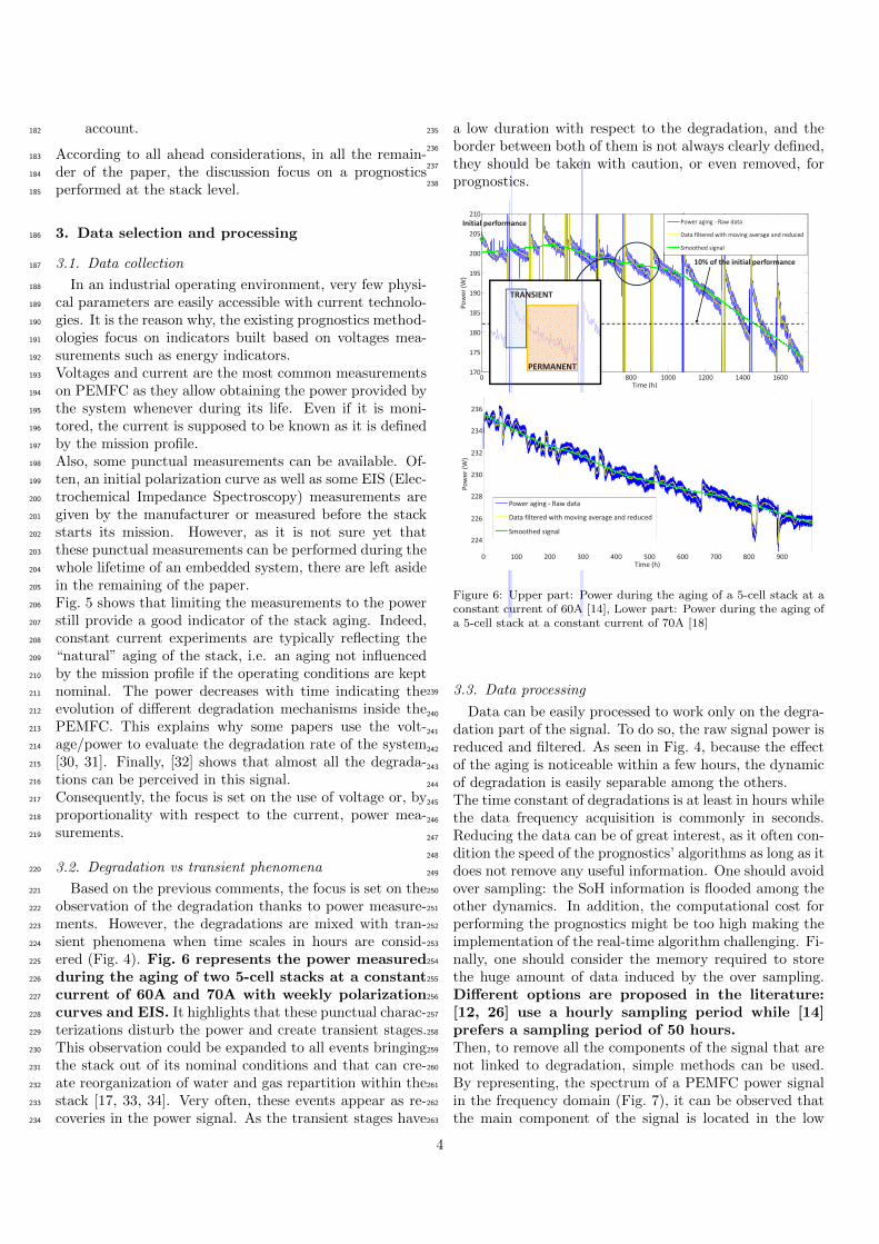
0.66

0.68

0.7

0.72

Time (h)

Vol

tage

(V)

Cell 1Cell 2Cell 3Cell 4Cell 5

0 200 400 600 800 1000 1200 1400 1600 18000

10

20

30

40

50

60

70

80

90

Time (h)

Load

(A)

Measured current I

0 200 400 600 800 1000 1200 1400 1600 18000

50

100

150

200

250

300

Time (h)

Pow

er (W

)

Stack PowerFigure 5: Individual cell voltages for a 5-cell stack aged at a constantcurrent of 60A [14]

Another perspective for prognostics may be being per-161

formed at a smaller level, namely the component level.162

It has already been initiated in [13] in which the size163

of the electrochemical active surface area (ECSA) is pre-164

dicted with a model-based prognostics framework. Many165

other critical parameters such as hydrogen crossover, re-166

sistances (or conductivities) or materials integrity could167

be predicted. Some failure thresholds have already been168

proposed for some of them. For instance, a crossover cur-169

rent of 10 mA.cm−2 is proposed in [29] as the EoL of the170

membrane subject to hydrogen crossover. However, differ-171

ent limitations appear when performing prognostics at the172

cell or components levels:173

1. the accessibility of the parameters: this point is dis-174

cussed in [8]. Accessing the inner parameters of the175

stack, when it is possible, almost always disturbs the176

stack behavior and tends to accentuate its degrada-177

tion;178

2. the lack of validated degradation models;179

3. the degradation at the interfaces between the compo-180

nents or with the auxiliaries may not be taken into181

3

account.182

According to all ahead considerations, in all the remain-183

der of the paper, the discussion focus on a prognostics184

performed at the stack level.185

3. Data selection and processing186

3.1. Data collection187

In an industrial operating environment, very few physi-188

cal parameters are easily accessible with current technolo-189

gies. It is the reason why, the existing prognostics method-190

ologies focus on indicators built based on voltages mea-191

surements such as energy indicators.192

Voltages and current are the most common measurements193

on PEMFC as they allow obtaining the power provided by194

the system whenever during its life. Even if it is moni-195

tored, the current is supposed to be known as it is defined196

by the mission profile.197

Also, some punctual measurements can be available. Of-198

ten, an initial polarization curve as well as some EIS (Elec-199

trochemical Impedance Spectroscopy) measurements are200

given by the manufacturer or measured before the stack201

starts its mission. However, as it is not sure yet that202

these punctual measurements can be performed during the203

whole lifetime of an embedded system, there are left aside204

in the remaining of the paper.205

Fig. 5 shows that limiting the measurements to the power206

still provide a good indicator of the stack aging. Indeed,207

constant current experiments are typically reflecting the208

“natural” aging of the stack, i.e. an aging not influenced209

by the mission profile if the operating conditions are kept210

nominal. The power decreases with time indicating the211

evolution of different degradation mechanisms inside the212

PEMFC. This explains why some papers use the volt-213

age/power to evaluate the degradation rate of the system214

[30, 31]. Finally, [32] shows that almost all the degrada-215

tions can be perceived in this signal.216

Consequently, the focus is set on the use of voltage or, by217

proportionality with respect to the current, power mea-218

surements.219

3.2. Degradation vs transient phenomena220

Based on the previous comments, the focus is set on the221

observation of the degradation thanks to power measure-222

ments. However, the degradations are mixed with tran-223

sient phenomena when time scales in hours are consid-224

ered (Fig. 4). Fig. 6 represents the power measured225

during the aging of two 5-cell stacks at a constant226

current of 60A and 70A with weekly polarization227

curves and EIS. It highlights that these punctual charac-228

terizations disturb the power and create transient stages.229

This observation could be expanded to all events bringing230

the stack out of its nominal conditions and that can cre-231

ate reorganization of water and gas repartition within the232

stack [17, 33, 34]. Very often, these events appear as re-233

coveries in the power signal. As the transient stages have234

a low duration with respect to the degradation, and the235

border between both of them is not always clearly defined,236

they should be taken with caution, or even removed, for237

prognostics.238

0 200 400 600 800 1000 1200 1400 1600170

175

180

185

190

195

200

205

210

Time (h)

Power(W

)

Power aging Raw data

Data filtered with moving average and reduced

Smoothed signal

TRANSIENT

PERMANENT

Initial performance

10% of the initial performance

0 100 200 300 400 500 600 700 800 900

224

226

228

230

232

234

236

Time (h)

Power(W

)

Power aging Raw data

Data filtered with moving average and reduced

Smoothed signal

Figure 6: Upper part: Power during the aging of a 5-cell stack at aconstant current of 60A [14], Lower part: Power during the aging ofa 5-cell stack at a constant current of 70A [18]

3.3. Data processing239

Data can be easily processed to work only on the degra-240

dation part of the signal. To do so, the raw signal power is241

reduced and filtered. As seen in Fig. 4, because the effect242

of the aging is noticeable within a few hours, the dynamic243

of degradation is easily separable among the others.244

The time constant of degradations is at least in hours while245

the data frequency acquisition is commonly in seconds.246

Reducing the data can be of great interest, as it often con-247

dition the speed of the prognostics’ algorithms as long as it248

does not remove any useful information. One should avoid249

over sampling: the SoH information is flooded among the250

other dynamics. In addition, the computational cost for251

performing the prognostics might be too high making the252

implementation of the real-time algorithm challenging. Fi-253

nally, one should consider the memory required to store254

the huge amount of data induced by the over sampling.255

Different options are proposed in the literature:256

[12, 26] use a hourly sampling period while [14]257

prefers a sampling period of 50 hours.258

Then, to remove all the components of the signal that are259

not linked to degradation, simple methods can be used.260

By representing, the spectrum of a PEMFC power signal261

in the frequency domain (Fig. 7), it can be observed that262

the main component of the signal is located in the low263

4

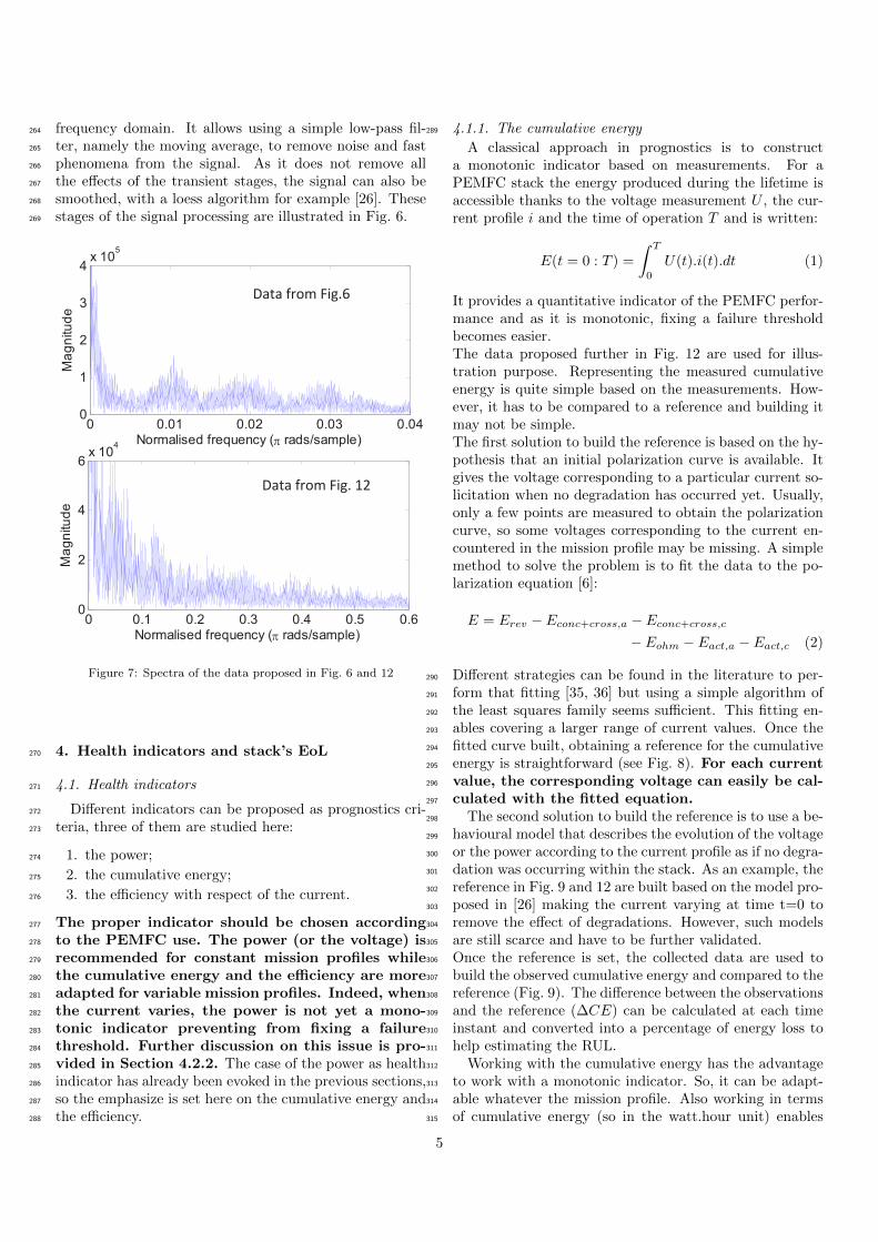
frequency domain. It allows using a simple low-pass fil-264

ter, namely the moving average, to remove noise and fast265

phenomena from the signal. As it does not remove all266

the effects of the transient stages, the signal can also be267

smoothed, with a loess algorithm for example [26]. These268

stages of the signal processing are illustrated in Fig. 6.269

q y ( p )

0 0.1 0.2 0.3 0.4 0.5 0.60

2

4

6x 10

4 P4: Données Propice

Normalised frequency ( rads/sample)

Ma

gn

itu

de

0 0.01 0.02 0.03 0.040

1

2

3

4x 10

5 P1: Données Régions

Normalised frequency ( rads/sample)

Ma

gn

itu

de

Data from Fig.6

Data from Fig. 12

Figure 7: Spectra of the data proposed in Fig. 6 and 12

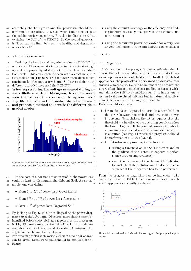
4. Health indicators and stack’s EoL270

4.1. Health indicators271

Different indicators can be proposed as prognostics cri-272

teria, three of them are studied here:273

1. the power;274

2. the cumulative energy;275

3. the efficiency with respect of the current.276

The proper indicator should be chosen according277

to the PEMFC use. The power (or the voltage) is278

recommended for constant mission profiles while279

the cumulative energy and the efficiency are more280

adapted for variable mission profiles. Indeed, when281

the current varies, the power is not yet a mono-282

tonic indicator preventing from fixing a failure283

threshold. Further discussion on this issue is pro-284

vided in Section 4.2.2. The case of the power as health285

indicator has already been evoked in the previous sections,286

so the emphasize is set here on the cumulative energy and287

the efficiency.288

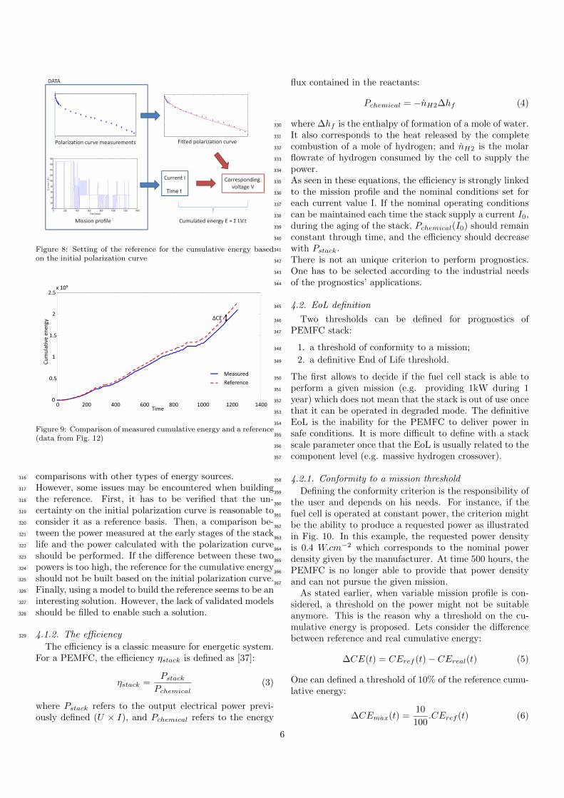
4.1.1. The cumulative energy289

A classical approach in prognostics is to constructa monotonic indicator based on measurements. For aPEMFC stack the energy produced during the lifetime isaccessible thanks to the voltage measurement U , the cur-rent profile i and the time of operation T and is written:

E(t = 0 : T ) =

∫ T

0

U(t).i(t).dt (1)

It provides a quantitative indicator of the PEMFC perfor-mance and as it is monotonic, fixing a failure thresholdbecomes easier.The data proposed further in Fig. 12 are used for illus-tration purpose. Representing the measured cumulativeenergy is quite simple based on the measurements. How-ever, it has to be compared to a reference and building itmay not be simple.The first solution to build the reference is based on the hy-pothesis that an initial polarization curve is available. Itgives the voltage corresponding to a particular current so-licitation when no degradation has occurred yet. Usually,only a few points are measured to obtain the polarizationcurve, so some voltages corresponding to the current en-countered in the mission profile may be missing. A simplemethod to solve the problem is to fit the data to the po-larization equation [6]:

E = Erev − Econc+cross,a − Econc+cross,c

− Eohm − Eact,a − Eact,c (2)

Different strategies can be found in the literature to per-290

form that fitting [35, 36] but using a simple algorithm of291

the least squares family seems sufficient. This fitting en-292

ables covering a larger range of current values. Once the293

fitted curve built, obtaining a reference for the cumulative294

energy is straightforward (see Fig. 8). For each current295

value, the corresponding voltage can easily be cal-296

culated with the fitted equation.297

The second solution to build the reference is to use a be-298

havioural model that describes the evolution of the voltage299

or the power according to the current profile as if no degra-300

dation was occurring within the stack. As an example, the301

reference in Fig. 9 and 12 are built based on the model pro-302

posed in [26] making the current varying at time t=0 to303

remove the effect of degradations. However, such models304

are still scarce and have to be further validated.305

Once the reference is set, the collected data are used to306

build the observed cumulative energy and compared to the307

reference (Fig. 9). The difference between the observations308

and the reference (∆CE) can be calculated at each time309

instant and converted into a percentage of energy loss to310

help estimating the RUL.311

Working with the cumulative energy has the advantage312

to work with a monotonic indicator. So, it can be adapt-313

able whatever the mission profile. Also working in terms314

of cumulative energy (so in the watt.hour unit) enables315

5

0 200 400 600 800 1000 1200 14000

20

40

60

80

100

120

140

160

180

Time (hours)

Cu

rre

nt

(A)

Current mission profile in A

Polarization curve measurements Fitted polarization curve

Mission profile

DATA

Current I

Time t

Corresponding

voltage V

Cumulated energy E = I.V.t

Figure 8: Setting of the reference for the cumulative energy basedon the initial polarization curve

0 200 400 600 800 1000 1200 14000

0.5

1

1.5

2

2.5x 109

Time

MeasuredReference

Cumulative en

ergy

ΔCE

Figure 9: Comparison of measured cumulative energy and a reference(data from Fig. 12)

comparisons with other types of energy sources.316

However, some issues may be encountered when building317

the reference. First, it has to be verified that the un-318

certainty on the initial polarization curve is reasonable to319

consider it as a reference basis. Then, a comparison be-320

tween the power measured at the early stages of the stack321

life and the power calculated with the polarization curve322

should be performed. If the difference between these two323

powers is too high, the reference for the cumulative energy324

should not be built based on the initial polarization curve.325

Finally, using a model to build the reference seems to be an326

interesting solution. However, the lack of validated models327

should be filled to enable such a solution.328

4.1.2. The efficiency329

The efficiency is a classic measure for energetic system.For a PEMFC, the efficiency ηstack is defined as [37]:

ηstack =Pstack

Pchemical(3)

where Pstack refers to the output electrical power previ-ously defined (U × I), and Pchemical refers to the energy

flux contained in the reactants:

Pchemical = −nH2∆hf (4)

where ∆hf is the enthalpy of formation of a mole of water.330

It also corresponds to the heat released by the complete331

combustion of a mole of hydrogen; and nH2 is the molar332

flowrate of hydrogen consumed by the cell to supply the333

power.334

As seen in these equations, the efficiency is strongly linked335

to the mission profile and the nominal conditions set for336

each current value I. If the nominal operating conditions337

can be maintained each time the stack supply a current I0,338

during the aging of the stack, Pchemical(I0) should remain339

constant through time, and the efficiency should decrease340

with Pstack.341

There is not an unique criterion to perform prognostics.342

One has to be selected according to the industrial needs343

of the prognostics’ applications.344

4.2. EoL definition345

Two thresholds can be defined for prognostics of346

PEMFC stack:347

1. a threshold of conformity to a mission;348

2. a definitive End of Life threshold.349

The first allows to decide if the fuel cell stack is able to350

perform a given mission (e.g. providing 1kW during 1351

year) which does not mean that the stack is out of use once352

that it can be operated in degraded mode. The definitive353

EoL is the inability for the PEMFC to deliver power in354

safe conditions. It is more difficult to define with a stack355

scale parameter once that the EoL is usually related to the356

component level (e.g. massive hydrogen crossover).357

4.2.1. Conformity to a mission threshold358

Defining the conformity criterion is the responsibility of359

the user and depends on his needs. For instance, if the360

fuel cell is operated at constant power, the criterion might361

be the ability to produce a requested power as illustrated362

in Fig. 10. In this example, the requested power density363

is 0.4 W.cm−2 which corresponds to the nominal power364

density given by the manufacturer. At time 500 hours, the365

PEMFC is no longer able to provide that power density366

and can not pursue the given mission.367

As stated earlier, when variable mission profile is con-sidered, a threshold on the power might not be suitableanymore. This is the reason why a threshold on the cu-mulative energy is proposed. Lets consider the differencebetween reference and real cumulative energy:

∆CE(t) = CEref (t) − CEreal(t) (5)

One can defined a threshold of 10% of the reference cumu-lative energy:

∆CEmax(t) =10

100.CEref (t) (6)

6

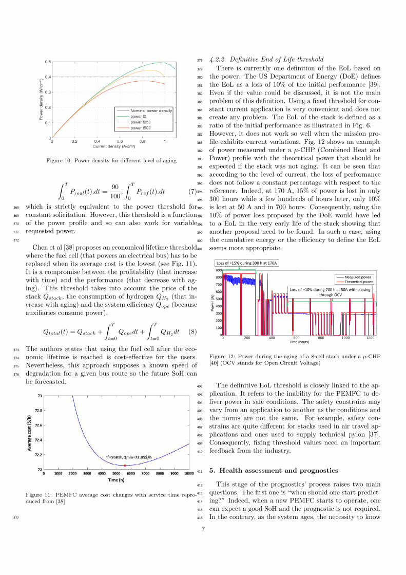
Figure 10: Power density for different level of aging

∫ T

0

Preal(t).dt =90

100.

∫ T

0

Pref (t).dt (7)

which is strictly equivalent to the power threshold for368

constant solicitation. However, this threshold is a function369

of the power profile and so can also work for variable370

requested power.371

372

Chen et al [38] proposes an economical lifetime thresholdwhere the fuel cell (that powers an electrical bus) has to bereplaced when its average cost is the lowest (see Fig. 11).It is a compromise between the profitability (that increasewith time) and the performance (that decrease with ag-ing). This threshold takes into account the price of thestack Qstack, the consumption of hydrogen QH2 (that in-crease with aging) and the system efficiency Qope (becauseauxiliaries consume power).

Qtotal(t) = Qstack +

∫ T

t=0

Qopedt+

∫ T

t=0

QH2dt (8)

The authors states that using the fuel cell after the eco-373

nomic lifetime is reached is cost-effective for the users.374

Nevertheless, this approach supposes a known speed of375

degradation for a given bus route so the future SoH can376

be forecasted.

Figure 11: PEMFC average cost changes with service time repro-duced from [38]

377

4.2.2. Definitive End of Life threshold378

There is currently one definition of the EoL based on379

the power. The US Department of Energy (DoE) defines380

the EoL as a loss of 10% of the initial performance [39].381

Even if the value could be discussed, it is not the main382

problem of this definition. Using a fixed threshold for con-383

stant current application is very convenient and does not384

create any problem. The EoL of the stack is defined as a385

ratio of the initial performance as illustrated in Fig. 6.386

However, it does not work so well when the mission pro-387

file exhibits current variations. Fig. 12 shows an example388

of power measured under a µ-CHP (Combined Heat and389

Power) profile with the theoretical power that should be390

expected if the stack was not aging. It can be seen that391

according to the level of current, the loss of performance392

does not follow a constant percentage with respect to the393

reference. Indeed, at 170 A, 15% of power is lost in only394

300 hours while a few hundreds of hours later, only 10%395

is lost at 50 A and in 700 hours. Consequently, using the396

10% of power loss proposed by the DoE would have led397

to a EoL in the very early life of the stack showing that398

another proposal need to be found. In such a case, using399

the cumulative energy or the efficiency to define the EoL400

seems more appropriate.401

0 200 400 600 800 1000 12000

100

200

300

400

500

600

700

800

900

Time (hours)

Pow

er (W

)

Measured powerTheoretical power

Loss of ≈15% during 300 h at 170A

Loss of ≈10% during 700 h at 50A with passingthrough OCV

Figure 12: Power during the aging of a 8-cell stack under a µ-CHP[40] (OCV stands for Open Circuit Voltage)

The definitive EoL threshold is closely linked to the ap-402

plication. It refers to the inability for the PEMFC to de-403

liver power in safe conditions. The safety constrains may404

vary from an application to another as the conditions and405

the norms are not the same. For example, safety con-406

strains are quite different for stacks used in air travel ap-407

plications and ones used to supply technical pylon [37].408

Consequently, fixing threshold values need an important409

feedback from the industry.410

5. Health assessment and prognostics411

This stage of the prognostics’ process raises two main412

questions. The first one is “when should one start predict-413

ing?” Indeed, when a new PEMFC starts to operate, one414

can expect a good SoH and the prognostic is not required.415

In the contrary, as the system ages, the necessity to know416

7

accurately the EoL grows and the prognostic should be417

performed more often, above all when coming closer to418

the sudden performance drop. But this implies to be able419

to define the SoH of the PEMFC. So the second question420

is “How can the limit between the healthy and degraded421

modes be set?”422

5.1. Health assessment423

Defining the healthy and degraded modes of a PEMFC is424

not trivial. The system starts degrading since its starting425

up and the power signal does not exhibit clear degrada-426

tion levels. This can clearly be seen with a constant cur-427

rent solicitation (Fig. 6) where the power starts decreasing428

continuously after only a few hours. So how to define the429

different degraded modes of the PEMFC?430

When representing the voltage measured during a431

stack lifetime with an histogram, it can be seen432

seen that different states seem to appear, see433

Fig. 13. The issue is to formalize that observation434

and propose a method to identify the different de-435

graded modes.436

Initial state

State evolution during the aging

Voltage (V)

Occurrence of a voltage value

Figure 13: Histogram of the voltages for a stack aged under a con-stant current profile (data from Fig. 6 lower part)

In the case of a constant mission profile, the power loss437

could be kept to distinguish the different SoH. As an ex-438

ample, one can define:439

• From 0 to 5% of power loss: Good health;440

• From 5% to 10% of power loss: Acceptable;441

• Over 10% of power loss: Degraded SoH.442

By looking at Fig. 6, this is not illogical as the power drop443

faster after the 10% limit. Of course, more classes might be444

identified before those 10%, as suggested by the histogram445

in Fig. 13. Some unsupervised classification methods are446

available, such as Hierarchical Ascendant Clustering [41,447

42], to refine the number of classes.448

For mission profiles with variable currents, no clear answer449

can be given. Some work trails should be explored in the450

future:451

• using the cumulative energy or the efficiency and find-452

ing different classes by analogy with the constant cur-453

rent example;454

• using the maximum power achievable for a very low455

or very high current value and following its evolution;456

• etc.457

5.2. Prognostics458

Let’s assume in this paragraph that a satisfying defini-459

tion of the SoH is available. A time instant to start per-460

forming prognostics should be decided. In all the published461

approaches, the prognostics is performed on datasets from462

finished experiments. So, the beginning of the predictions463

is very often chosen to get the best prediction horizon with-464

out taking the SoH into consideration. It is important to465

test and validate the algorithms but in industrial applica-466

tions, this practice is obviously not possible.467

Two possibilities appear:468

1. for model-based approaches: setting a threshold on469

the error between theoretical and real stack power470

in percent. Nevertheless, the latter requires that the471

threshold is a function of the operating conditions (see472

the loss on Fig. 12). If the residual crosses a threshold,473

an anomaly is detected and the prognostic procedure474

is executed (see Fig. 14 where the prognostic should475

be performed at t = 38s) [43, 44].476

2. for data-driven approaches, two solutions:477

• setting a threshold on the SoH indicator and on478

the gradient of the latter (to capture a perfor-479

mance drop or improvement);480

• using the histogram of the chosen SoH indicator481

to track the state evolution and to decide in con-482

sequence if the prognostic has to be performed.483

Then the prognostics algorithm can be launched. The484

reader can refer to Table 1 for more information on dif-485

ferent approaches currently available.486

0 10 20 30 40 50 60 70 804

3

2

1

0

1

2

3

4

5

6

7

Time (s)

Residual

Threshold

Residual

Threshold

Figure 14: A residual and thresholds to trigger the prognostics pro-cedure

8

Table 1: Characteristics of a few works developed in the field of PEMFC prognostics

Year Reference Type Health indicator State estimation and/or prognostics tools2012 [13] model-based Stack voltage (1-cell stack,

I variable)Unscented Kalman Filter

2014

[17] data-driven Stack voltage (I constant) Particle filter[14] data-driven Mean cell voltage (I con-

stant)Echo State Network

[15] data-driven Stack voltage (I constant) Adaptive Neuro Fuzzy Inference Systems[19] data-driven Impedance Equivalent circuit[20] data-driven Impedance Regressions[21] data-driven Stack voltage (I constant) Regime switching vector autoregressive

(RSVAR)[22] data-driven Stack voltage (I constant) Particle filter

2015

[16] data-driven Stack voltage (I constant) Summation-Wavelet Extreme Learning Ma-chine

[12] model-based Stack voltage (I variable) Kalman Filter[11] model-based Impedance and polariza-

tion curvesRegressions

[45] Hybrid Stack voltage (I variable) Particle filter

6. Evaluating prognostics’ performance487

6.1. Prediction horizon488

It is important to evaluate the duration needed between489

the prediction instant and the decision and/or action in-490

stant. The horizon may depend on the goal of prognostics.491

Consequently, the reasoning is proposed on an example,492

and can be transposed in other applications.493

Let’s take the example of the maintenance rescheduling for494

a transportation or a µ-CHP PEMFC. It is assumed that495

the mission rescheduling can be done remotely, so only the496

maintenance constraints impact the prediction horizon ex-497

pected. To perform maintenance, different time durations498

have to be taken into account: (1) the planning of the499

maintenance operations, 1-2 days; (2) the delay to obtain500

spare parts, 10-20 days; (3) the maintenance realization,501

1-7 days. It gives a total duration between 12 and 29 days.502

It means that the prognostics should give results with a503

horizon between 300 and 700 hours to be considered as504

a good performance. Obviously, this time interval should505

be discussed with respect to industrial feedbacks in the506

future.507

6.2. Acceptable error on RUL estimates508

Regarding the RUL estimates, there are two cases: (1)509

the estimate is smaller than the actual RUL, it is an early510

prediction, or (2) the estimate is greater, it is a late predic-511

tion. The acceptable error cannot be the same in each case.512

Indeed, by validating a prediction with a consequent delay,513

one may risk a complete shutdown of its power source. It514

is intolerable in most PEMFC applications. Consequently,515

according to the horizon discussed earlier, it is proposed to516

allow a maximum delay of one day. It represent an error517

of 8% for a horizon of 300 hours.518

The case of the early prediction allows more flexibility.519

Anticipating a maintenance is less disadvantageous than520

being late, even if it can create some extra costs due to521

the replacement of a functioning system. It is proposed to522

set the early prediction limit at 16% of the actual RUL,523

whatever the time instant. It represents 48h for a horizon524

of 300h and 4 days (112h) for a horizon of 700 hours. The525

acceptable error is depicted in Fig. 15.526

RUL

Time 

24h ≈ 8%

Acceptable error

48h ≈ 16%

300 h

Actual RULConfidence bounds 

Figure 15: Acceptable error on RUL estimates

6.3. Acceptable uncertainty527

Defining the uncertainty allowed in the prediction is not528

trivial as no standards are available for PEMFC on that529

subject. So let’s try to reason on the current standard on530

electricity production.531

Nowadays, electricity suppliers in Europe have to provide532

a voltage of 230 V ±10% (at 50 Hz) [46]. This constrain533

evolves according to the world location. In North America,534

the standard impose a nominal voltage of 120 V with a535

tolerance of ±5% (at 60 Hz) [47]. Even if, the standards536

9

are not uniform, they can be used to propose a confidence537

interval objective for prognostics. Indeed, to ensure that538

the prognostics’ results are reliable anywhere in the word,539

the uncertainty on the SoH or RUL estimates should be540

constrained in a ±5% interval. Nevertheless, a confidence541

interval of ±10% allows to assert that the predictions are542

quite satisfying but can be improved. Again, industrial543

feedbacks are necessary to discuss further on that subject.544

7. Conclusion545

Developing prognostics for PEMFC can be a solution546

to contribute to extend the system’s lifetime. However,547

the lack of standards to guide current works may lead to548

the appearance of prognostics’ proposals with very poor549

adaptation capacities to actual industrial situations. To550

start a discussion on this subject, this paper proposes guid-551

ance on several aspects such as state definition, selection552

of prognostics’ criteria or performance evaluation. This is553

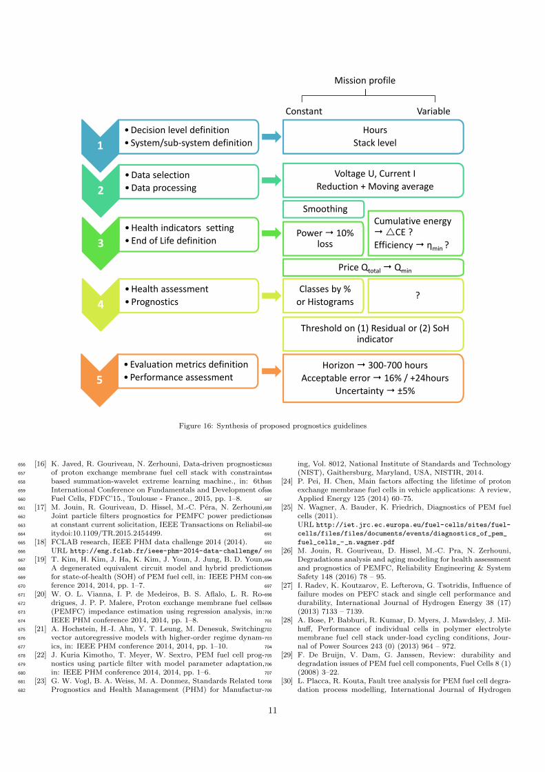
synthesized in Fig. 16.554

This work first shows how important it is to set the555

hypotheses of the prognostics application. Indeed, it lim-556

its the prognostics’ approach to specific real life cases of557

PEMFC applications. Also, it makes appear some techno-558

logical constrains, as the types of measurements available,559

as well as indications on the phenomena that should be560

taken into account (transient and/or permanent regimes).561

To evaluate the current and future state of health of the562

system, it is important to know if the stack remains in an563

healthy mode or already is in a degraded one. There is564

currently no clear borders between these states. Defining565

which ones are degraded states is still to debate.566

Performing predictions requires health indicators. Accord-567

ing to the application, the criteria might be different and568

this leads to the proposal of several indicators such as the569

power, the cumulative energy and the efficiency. All de-570

pend on the mission profile and the pathway from one571

to another can be easily made. However, defining failure572

thresholds related to each criterion remains an open ques-573

tion. Moreover, this lead to wonder how the end of life of574

the stack is defined. Two solutions are proposed related575

first to the mission in progress and then related to an in-576

ability of the stack to provide power in safe conditions.577

Finally, to help validating prognostics approaches, some578

performance metrics are proposed and discussed. They579

try to take into account real life constrains such as electri-580

cal norms and maintenance delays. Nevertheless, the lack581

of industrial feedback in the literature prevents a precise582

discussion on the subject.583

To extend the proposals from this paper to short-584

term predictions for adaptive control, small time585

scales, as a minute, will have be studied and dis-586

cussed. As it may raise issue linked to the speed of587

the algorithm or the accuracy needed to use short-588

term predictions for example, this stage might wait589

that more prognostics’ approaches are available in590

the literature. The field of prognostics of PEMFC has591

just started and a great reflection effort is needed to de-592

velop approaches that, one day, can be transferable to the593

industry.594

8. Acknowledgments595

The authors would like to thank the ANR project596

PROPICE (ANR-12-PRGE-0001) and the Labex AC-597

TION project (contract ”ANR-11-LABX-01-01”) both598

funded by the French National Research Agency as well599

as the French region of Franche-Comte for their support.600

References601

[1] X. Luo, J. Wang, M. Dooner, J. Clarke, Overview of current602

development in electrical energy storage technologies and the603

application potential in power system operation, Applied En-604

ergy 137 (2015) 511–536.605

[2] Y. Wanga, K. S. Chen, J. Mishler, S. C. Cho, X. C. Adroher,606

A review of polymer electrolyte membrane fuel cells: Technol-607

ogy, applications, and needs on fundamental research, Applied608

Energy 88 (2011) 981–1007.609

[3] S.-D. Oh, K.-Y. Kim, S.-B. Oh, H.-Y. Kwak, Optimal operation610

of a 1-kw pemfc-based chp system for residential applications,611

Applied Energy 96 (2012) 93–101.612

[4] J. Fernandez-Moreno, G. Guelbenzu, A. Martin, M. Folgado,613

P. Ferreira-Aparicio, A. Chaparro, A portable system powered614

with hydrogen and one single air-breathing pem fuel cell, Ap-615

plied Energy 109 (2013) 60–66.616

[5] E4tech, The fuel cell industry review 2014 (Nov. 2014).617

URL http://www.fuelcells.org/pdfs/TheFuelCellIndustry618

Review2014.pdf619

[6] O. Z. Sharaf, M. F. Orhan, An overview of fuel cell technology:620

Fundamentals and applications, Renewable and Sustainable En-621

ergy Reviews 32 (2014) 810 – 853.622

[7] G. Niu, D. Anand, M. Pecht, Prognostics and health manage-623

ment for energetic material systems, in: Prognostics and Health624

Management Conference, 2010. PHM ’10., 2010, pp. 1–7.625

[8] M. Jouin, R. Gouriveau, D. Hissel, M.-C. Pera, N. Zerhouni,626

Prognostics and health management of PEMFC state of the627

art and remaining challenges, International Journal of Hydrogen628

Energy 38 (35) (2013) 15307 – 15317.629

[9] J. W. Sheppard, M. A. Kaufman, T. J. Wilmer, IEEE stan-630

dards for prognostics and health management, Aerospace and631

Electronic Systems Magazine, IEEE 24 (9) (2009) 34–41.632

[10] ISO13381-1, Condition monitoring and diagnostics of machines633

- prognostics - Part1: General guidelines, International Stan-634

dard, ISO, 2004.635

[11] E. Lechartier, E. Laffly, M.-C. Pera, R. Gouriveau, D. Hissel,636

N. Zerhouni, Proton exchange membrane fuel cell behavioral637

model suitable for prognostics, International Journal of Hydro-638

gen Energy 40 (26) (2015) 8384–8397.639

[12] M. Bressel, M. Hilairet, D. Hissel, B. O. Bouamama, Extended640

kalman filter for prognostic of proton exchange membrane fuel641

cell, Applied Energy 164 (2016) 220 – 227.642

[13] X. Zhang, P. Pisu, An unscented kalman filter based approach643

for the health-monitoring and prognostics of a polymer elec-644

trolyte membrane fuel cell, in: Proceedings of the annual con-645

ference of the prognostics and health management society, 2012.646

[14] S. Morando, S. Jemei, R. Gouriveau, D. Hissel, N. Zer-647

houni, Fuel cells remaining useful lifetime forecasting using echo648

state network, in: Vehicle Power and Propulsion Conference649

(VPPC’14), 2014, pp. IS1–4.650

[15] R. Silva, R. Gouriveau, S. Jemei, D. Hissel, L. Boulon, K. Ag-651

bossou, N. Y. Steiner, Proton exchange membrane fuel cell652

degradation prediction based on adaptive neuro fuzzy infer-653

ence systems, International Journal of Hydrogen Energy 39 (21)654

(2014) 11128 – 11144.655

10

1•Decision level definition• System/sub‐system definition

2•Data selection•Data processing

3•Health indicators setting• End of Life definition

4•Health assessment•Prognostics

5•Evaluation metrics definition•Performance assessment

HoursStack level

Voltage U, Current IReduction + Moving average

Power  10% loss

Classes by %or Histograms

Horizon  300‐700 hoursAcceptable error 16% / +24hours

Uncertainty ±5%

Mission profile

Variable 

SmoothingCumulative energyCE ?Efficiency ηmin ?

Price Qtotal Qmin

?

Threshold on (1) Residual or (2) SoHindicator

Constant 

Figure 16: Synthesis of proposed prognostics guidelines

[16] K. Javed, R. Gouriveau, N. Zerhouni, Data-driven prognostics656

of proton exchange membrane fuel cell stack with constraint657

based summation-wavelet extreme learning machine., in: 6th658

International Conference on Fundamentals and Development of659

Fuel Cells, FDFC’15., Toulouse - France., 2015, pp. 1–8.660

[17] M. Jouin, R. Gouriveau, D. Hissel, M.-C. Pera, N. Zerhouni,661

Joint particle filters prognostics for PEMFC power prediction662

at constant current solicitation, IEEE Transactions on Reliabil-663

itydoi:10.1109/TR.2015.2454499.664

[18] FCLAB research, IEEE PHM data challenge 2014 (2014).665

URL http://eng.fclab.fr/ieee-phm-2014-data-challenge/666

[19] T. Kim, H. Kim, J. Ha, K. Kim, J. Youn, J. Jung, B. D. Youn,667

A degenerated equivalent circuit model and hybrid prediction668

for state-of-health (SOH) of PEM fuel cell, in: IEEE PHM con-669

ference 2014, 2014, pp. 1–7.670

[20] W. O. L. Vianna, I. P. de Medeiros, B. S. Aflalo, L. R. Ro-671

drigues, J. P. P. Malere, Proton exchange membrane fuel cells672

(PEMFC) impedance estimation using regression analysis, in:673

IEEE PHM conference 2014, 2014, pp. 1–8.674

[21] A. Hochstein, H.-I. Ahn, Y. T. Leung, M. Denesuk, Switching675

vector autoregressive models with higher-order regime dynam-676

ics, in: IEEE PHM conference 2014, 2014, pp. 1–10.677

[22] J. Kuria Kimotho, T. Meyer, W. Sextro, PEM fuel cell prog-678

nostics using particle filter with model parameter adaptation,679

in: IEEE PHM conference 2014, 2014, pp. 1–6.680

[23] G. W. Vogl, B. A. Weiss, M. A. Donmez, Standards Related to681

Prognostics and Health Management (PHM) for Manufactur-682

ing, Vol. 8012, National Institute of Standards and Technology683

(NIST), Gaithersburg, Maryland, USA, NISTIR, 2014.684

[24] P. Pei, H. Chen, Main factors affecting the lifetime of proton685

exchange membrane fuel cells in vehicle applications: A review,686

Applied Energy 125 (2014) 60–75.687

[25] N. Wagner, A. Bauder, K. Friedrich, Diagnostics of PEM fuel688

cells (2011).689

URL http://iet.jrc.ec.europa.eu/fuel-cells/sites/fuel-690

cells/files/files/documents/events/diagnostics_of_pem_691

fuel_cells_-_n.wagner.pdf692

[26] M. Jouin, R. Gouriveau, D. Hissel, M.-C. Pra, N. Zerhouni,693

Degradations analysis and aging modeling for health assessment694

and prognostics of PEMFC, Reliability Engineering & System695

Safety 148 (2016) 78 – 95.696

[27] I. Radev, K. Koutzarov, E. Lefterova, G. Tsotridis, Influence of697

failure modes on PEFC stack and single cell performance and698

durability, International Journal of Hydrogen Energy 38 (17)699

(2013) 7133 – 7139.700

[28] A. Bose, P. Babburi, R. Kumar, D. Myers, J. Mawdsley, J. Mil-701

huff, Performance of individual cells in polymer electrolyte702

membrane fuel cell stack under-load cycling conditions, Jour-703

nal of Power Sources 243 (0) (2013) 964 – 972.704

[29] F. De Bruijn, V. Dam, G. Janssen, Review: durability and705

degradation issues of PEM fuel cell components, Fuel Cells 8 (1)706

(2008) 3–22.707

[30] L. Placca, R. Kouta, Fault tree analysis for PEM fuel cell degra-708

dation process modelling, International Journal of Hydrogen709

11

Energy 36 (19) (2011) 12393 – 12405.710

[31] X. Zhang, Y. Rui, Z. Tong, X. Sichuan, S. Yong, N. Huaisheng,711

The characteristics of voltage degradation of a proton exchange712

membrane fuel cell under a road operating environment, In-713

ternational Journal of Hydrogen Energy 39 (17) (2014) 9420 –714

9429.715

[32] A. Franco, Modelling and analysis of degradation phenomena716

in pemfc, Woodhead, 2012.717

[33] S. Kundu, M. Fowler, L. C. Simon, R. Abouatallah, Reversible718

and irreversible degradation in fuel cells during open circuit719

voltage durability testing, Journal of Power Sources 182 (1)720

(2008) 254 – 258.721

[34] J. Wu, X.-Z. Yuan, J. J. Martin, H. Wang, D. Yang, J. Qiao,722

J. Ma, Proton exchange membrane fuel cell degradation under723

close to open-circuit conditions: Part I: In situ diagnosis, Jour-724

nal of Power Sources 195 (4) (2010) 1171 – 1176.725

[35] A. Askarzadeh, Parameter estimation of fuel cell polarization726

curve using BMO algorithm, International Journal of Hydrogen727

Energy 38 (35) (2013) 15405 – 15413.728

[36] M. Santarelli, M. Torchio, P. Cochis, Parameters estimation of729

a PEM fuel cell polarization curve and analysis of their behavior730

with temperature, Journal of Power Sources 159 (2) (2006) 824731

– 835.732

[37] M.-C. Pera, D. Hissel, H. Gualous, C. Turpin, Fuel733

Cells, John Wiley & Sons, Inc., 2013, pp. 151–207.734

doi:10.1002/9781118576892.ch3.735

[38] H. Chen, P. Pei, M. Song, Lifetime prediction and the economic736

lifetime of proton exchange membrane fuel cells, Applied Energy737

142 (2015) 154–163.738

[39] U. D. of Energy, The department of energy hydrogen and fuel739

cells program plan (2011).740

URL http://www.hydrogen.energy.gov/roadmaps\_vision.h741

tml742

[40] E. Pahon, S. Morando, R. Petrone, al., Long-term tests duration743

reduction for pemfc µ-chp application, in: ICREGA16, 2016,744

pp. 1–6.745

[41] J. H. Ward Jr, Hierarchical grouping to optimize an objec-746

tive function, Journal of the American statistical association747

58 (301) (1963) 236–244.748

[42] T. Aroui, Y. Koubaa, A. Toumi, Self-organizing maps for di-749

agnosing induction motors supplied by a variable speed drive,750

European journal of electrical engineering 14 (6) (2011) 697–751

717.752

[43] B. O. Bouamama, M. Bressel, D. Hissel, M. Hilairet, Robust753

diagnosability of PEMFC based on bond graph LFT, ICECE754

2015: International Conference on Electrical and Control Engi-755

neering 2 (6) (2015) 1197.756

[44] M. Djeziri, B. O. Bouamama, R. Merzouki, Modelling and ro-757

bust FDI of steam generator using uncertain bond graph model,758

Journal of Process Control 19 (1) (2009) 149–162.759

[45] M. Jouin, R. Gouriveau, D. Hissel, M.-C. Pera, N. Zerhouni,760

Prognostics of PEM fuel cells under a combined heat and power761

profile, in: Proceedings of the 2015 IFAC Symposium on Infor-762

mation Control in Manufacturing (INCOM 2015), 2015.763

[46] CENELEC, European committee for electrotechnical standard-764

ization, http://www.cenelec.eu/index.html.765

[47] NEMA, American national standard for electric power766

systems and equipment voltage ratings (60 hz),767

http://www.nema.org/Standards/Pages/American-National-768

Standard-for-Electric-Power-Systems-and-Equipment-769

Voltage-Ratings.aspx.770

12