Estimating the Dynamics of Mutual Fund Alphas … the... · Estimating the Dynamics of Mutual Fund...

Estimating the Dynamics of Mutual FundAlphas and Betas

Harry MamayskyOld Lane LP

Matthew SpiegelYale School of Management

Hong ZhangINSEAD, Singapore

This article develops a Kalman filter model to track dynamic mutual fund factorloadings. It then uses the estimates to analyze whether managers with market-timingability can be identified ex ante. The primary findings are as follows: (i) Ordinaryleast squares (OLS) timing models produce false positives (nonzero alphas) at toohigh a rate with either daily or monthly data. In contrast, the Kalman filter modelproduces them at approximately the correct rate with monthly data; (ii) In monthlydata, though the OLS models fail to detect any timing among fund managers, theKalman filter does; (iii) The alpha and beta forecasts from the Kalman model are moreaccurate than those from the OLS timing models; (iv) The Kalman filter model tracksmost fund alphas and betas better than OLS models that employ macroeconomicvariables in addition to fund returns. (JEL G12, G14, G23, C01, C12, C13, C52, C53)

A great deal of attention has gone into understanding mutual fundreturns and trading strategies.1 What most studies have in common is themaintained hypothesis that their returns can be represented by a staticordinary least squares (OLS) model.2 Although this may be a reasonableconjecture for some funds, it seems unlikely to be true for many others.

The authors thank Robert Engle, Wayne Ferson, Will Goetzmann, and Geert Rouwenhorst for theircomments. We would like to thank participants at the Rutgers Conference honoring David Whitcomb,the 2004 Meetings of the American Finance Association, and seminar participants at Boston College andthe University of Wisconsin-Madison. Hong Zhang thanks the INSEAD Alumni Fund (IAF) for financialsupport. We also thank two anonymous referees and the editor Cam Harvey for their comments that led tothe article’s investigation of market-timing measures. Address correspondence to Matthew Spiegel, YaleSchool of Management, P.O. Box 208200, New Haven, CT 06520, or e-mail: [email protected].

1 Examples of the former include Lehmann and Modest (1987), Grinblatt and Titman (1992), Hendricks,Patel, and Zeckhauser (1993), Brown and Goetzmann (1995), Carhart (1997), Daniel et al. (1997), Wermers(2000), Pastor and Stambaugh (2002), and Teo and Woo (2001). Examples of the latter include Fersonand Schadt (1996), Brown and Goetzmann (1997), and Ferson and Khang (2002).

2 One exception is Grinblatt and Titman (1994). The methodology they use avoids a direct comparisonagainst a specific portfolio, and instead uses an ‘‘endogenous’’ benchmark. However, their techniquerequires knowledge of the fund’s actual composition, which may not always be available. Ferson andKhang (2002) extend the technique to condition the portfolio betas on exogenous variables such asmacroeconomic data.

© The Author 2007. Published by Oxford University Press on behalf of The Society for Financial Studies.All rights reserved. For Permissions, please email: [email protected]:10.1093/rfs/hhm049

at Tsinghua U

niversity on Decem

ber 2, 2014http://rfs.oxfordjournals.org/

Dow

nloaded from

http://rfs.oxfordjournals.org/

The Review of Financial Studies / v 00 n 0 2007

Investors presumably employ portfolio managers to move assets into andout of various sectors and securities as part of a dynamic strategy. This isespecially true if they hope to employ managers with market-timing skills.If so, detecting managerial timing ability with a static statistical model maylead to false positives at an unexpectedly high rate. The analysis presentedhere confirms that this is indeed a problem and shows how a dynamicKalman filter model can be employed to ameliorate it successfully and findmangers who appear to have a genuine ability to time the market.

This article extends the mutual fund performance literature along thelines of Ferson and Schadt (1996) (hereafter FS). The FS techniqueis designed to estimate the manager’s implicit strategy with respect tomacro variables and then allow for the resulting correlations when judgingperformance.3 However, in contrast to FS, our goal is to allow forportfolio shifts due to factors unobservable by the econometrician. Thisis accomplished by assuming that assets are reallocated on the basis ofsome unobserved factor, and then estimating the system of equations via aKalman filter. Of course, one can also include the macroeconomic factorsFS use, thereby allowing for both observable and unobservable factors inthe specification.

This article demonstrates the Kalman filter model’s ability to handledynamic factor loadings by estimating it on U.S. mutual fund data. Theresulting alpha and beta time series show that many funds do indeedfollow highly dynamic strategies. Using the monthly data, a subset of them(perhaps as high as 20%) is also shown to possess market-timing ability.This contrasts with Bollen and Busse (2001) (hereafter BB) who, using theOLS models proposed by Treynor and Mazuy (1966) and Henriksson andMerton (1981), do not find such ability with monthly data. The differencelies in the Kalman filter model’s ability to adapt to a fund’s current loadingon market risk in a way that a rolling OLS model cannot.

The results presented here also question the usefulness of using dailydata for analyzing mutual fund performance. As BB note, the daily datado potentially offer researchers additional power.4 But, this potential alsocomes with a number of microstructure problems like stale pricing andbid–ask bounce. Tests presented here indicate that such problems mayindeed impact market-timing estimates.

On average, as a fund’s estimated market-timing skill increaseswith regard to current period returns, the analogous skill estimates

3 Several recent articles have adopted this technique for performance evaluation. For example, seeChristopherson, Ferson, and Glassman (1998), and Blake, Lehmann, and Timmermann (2002).

4 BB create passive characteristic matched control portfolios for the managed funds in their dataset. Theythen find that with daily data the managed funds produce larger market-timing parameters than thecontrol funds. In contrast, using monthly data they fail to detect any statistical difference between thecontrol portfolios and the managed funds. From this the paper concludes that with daily data one can findevidence of market-timing ability among fund managers. The monthly data, in their view, do not generatethe same result owing to a lack of power generated by the infrequent sampling interval.

2

2008The Review of Financial Studies / v 21 n1

234

at Tsinghua U

niversity on Decem


Dow

nloaded from


Estimating the Dynamics of Mutual Fund Alphas and Betas

using lagged returns decrease. In the absence of microstructure problems,the lagged returns should produce uncorrelated parameter estimatesbecause lagged returns should be uncorrelated with current returns.However, if microstructure issues have generated a false-positive market-timing ability parameter, the lagged return coefficients then act to offset it.The results presented here are consistent with this hypothesis: a nonzerocurrent-period market-timing parameter is associated with lagged timingparameters of about equal size and opposite sign.

As noted by Jagannathan and Korajczyk (1986) an examination of theTreynor and Mazuy (1966) (hereafter TM) and Henriksson and Merton(1981) (hereafter HM) parameter estimates shows that they tend to tradeoff errors in the market-timing parameter with errors in the estimated fundalphas.5 In this case, high market-timing estimates are highly correlatedwith low estimated alphas. This implies that testing a model’s factorforecasts one factor at a time may miss problems in other factors.Conversely, it is also possible for a model’s overall forecasting powerto be good even if the underlying factor estimates appear questionable. Tocheck for these possibilities this article uses a test suggested by Bollen andBusse (2005) and an omnibus test developed here that controls for all of amodel’s factors at once.

The omnibus test, rather than conducting the usual sorts, creates fund-by-fund zero-alpha zero-beta portfolios by going long the fund and shortthe factors based on each model’s forecasts. An ideal model should produceout-of-sample factor loadings centered on zero for these portfolios. TheTM, HM, and four-factor Kalman models fail this test. One mightconjecture that the OLS-based HM and TM models would do well ifestimated only on funds with low turnover rates. They do not. In contrast,though, the out-of-sample portfolio statistics produced by the one-factorKalman model cover zero within the 95% bootstrapped confidence intervalfor the sample as a whole and each turnover tercile. This implies that theone-factor Kalman filter model does not create spurious parameters butinstead provides a useful signal regarding a fund’s timing ability and itsfuture factor loadings.

The final test in the article looks at the degree to which usingconditioning information, as in FS, adds to the model’s ability to fitthe data within sample. Overall, the conditioning information does notimprove the model’s fit (as measured by the R2 statistic). But this is nottrue of every fund. The number of funds with significant parameter valuessomewhat exceeds the number that would be produced by chance. Froman economic point of view, these findings indicate that even though some

5 The HM model adds γ rmtI {rmt > 0} to the standard factor model as a means of detecting market-timingability. Here, rmt is the market return net of the risk-free rate, and I {rmt > 0}is an indicator function thatequals 1 when rmt > 0 and zero otherwise. The TM model replaces γ rmtI {rmt > 0} with γ r2

mt.

3235

at Tsinghua U

niversity on Decem


Dow

nloaded from



funds condition on the type of macro information tested here, many donot. For those that do not, the Kalman filter picks up the time variationin their betas and alphas via estimates of the unobserved factor’s value.The tests in this article suggest that up to 20% of all mutual funds (using a5% critical value) exhibit investment strategies with some dependence onthe lagged treasury-bill rate, and on the market dividend yield. Of course,the other funds may be conditioning on macro information not includedin this article’s tests, a possibility that offers intriguing avenues for futureresearch.

The remainder of the article proceeds as follows. Section 1 describesthe data used to estimate the model. Section 2 derives the Kalman filtermodel that this article proposes and an alternative empirical specificationfor tracking dynamic alphas and betas. Section 3 conducts a series of out-of-sample tests to check for the reliability of the estimates generated by themodels examined here. Section 4 develops and provides an omnibus testof each model’s overall ability to provide accurate forecasts. Section5 examines the reasonableness of the estimated parameter dynamicsproduced with the Kalman filter model. Section 6 explores the impactof adding macroeconomic factors like those used in FS to the model.Section 7 concludes.

1. Data Description and Model Estimation

Monthly mutual fund data from 1970 to 2002 come from Center forResearch in Security Prices (CRSP). A fund is included only if it hasmore than 48 months of return data. Daily mutual fund data come froma now-defunct firm called Wall Street Web (WSW).6 The data begin onJuly 25, 1962 and end on October 5, 2004. Once multiple-share class fundsare consolidated, up to 1998, the overlap between the CRSP and WSWdata averages just over 90%. After that the overlap declines, but onlybecause the WSW database ceases to include new funds. Examining thetotal returns for funds that are in both the CRSP daily database and theWSW database shows that they are identical up to some small roundingerrors. Finally, a comparison of the equally weighted monthly fund returnsfrom both files yields a correlation coefficient of 0.9977 before 1999.

Other data include the market, Treasury bill, Fama-French factors,momentum (MOM) factor, and CRSP stock decile returns. The empiricalsection comparing the Kalman filter to the FS conditional model alsouses the lagged dividend yield on the market. The monthly dividend yieldequals the CRSP value-weighted index total return with dividends, minusthe return without dividends. The lagged dividend yield is then calculatedas the average of these monthly values in the previous calendar year.

6 The database is currently housed at the Yale School of Management’s International Center for Finance.

4


236

at Tsinghua U

niversity on Decem


Dow

nloaded from



Although many studies such as Grinblatt and Titman (1993), Danielet al. (1997), and Cohen, Coval, and Pastor (2005) have used the mutualfund holdings data with great success, this database is not used here.The reason for this disparity is that papers based on the holdings dataseek to detect, prior to fees and other expenses, whether managers havethe ability to select stocks that will produce above-market, risk-adjustedreturns. Here, however, the focus is on whether managers have market-timing ability and if this ability can be reliably detected. Unfortunately,the relative infrequency with which fund holdings are sampled makes theiruse in this article’s context difficult. Nevertheless, tests were conducted tosee if these data could be used to detect market-timing ability among fundmangers. Because all the results were negative, they are not reported here.

2. Derivation of the Kalman Filter Model

Every statistical model generates false positives. In fact, the statement thata coefficient is ‘‘significant at the X% level’’ recognizes that X% of thetime the statistical model will yield a false-positive result. However, whileone must accept that any model will yield false positives, the model shouldnot do so more frequently than one expects, given a particular criticalvalue. Studies including those by Jagannathan and Korajczyk (1986) andBollen and Busse (2001) show that with real data the HM and TM modelsgenerate false positives on the model’s timing coefficient (labeled γ in thisstudy) at a rate that is far too high.7 Thus, the question is whether itis possible to produce an alternative model capable of detecting markettiming that does not suffer from this problem.

A generic problem with the OLS model is that the constant factor-loading assumption is likely to be violated for managed portfolios,especially if managers are attempting to time the market. This meansthat such models are inherently misspecified and are thus likely to produceunexpected results—a tendency to produce false positives, for example.One potential solution is to derive a dynamic model and use it to test formanagerial market-timing ability.

If fund managers are to outperform the market on a risk-adjustedbasis, they must receive some sort of private signal that forecasts returns.To accommodate this, one needs to start with a general equilibriummodel of asset returns with asymmetric information such as Admati(1985). Extending the basic setting to a multiple-period framework, from aparticular fund manager’s perspective the return on asset i can be describedby a linear factor model with constant factor loadings:

rit − rf = αit + β ′i (rmt − rf ) + εit. (1)

7 In addition to the standard factors, the HM and TM models produce a market-timing coefficient. Thoseinterested in further details should consult the original articles.

5237

at Tsinghua U

niversity on Decem


Dow

nloaded from



The risk-adjusted abnormal return αit depends upon the current value ofthe manager’s signal. Technically, therefore, it should include a parameterindicating the signal upon which it is based. However, for the sake ofnotational simplicity it is not displayed here. Under the null hypothesis(which will be formally developed later on) the manager’s signal does notforecast stock returns, and the α-terms are zero. Throughout this article itis assumed that the errors are normally distributed and independent overtime. Note that although returns change over time, their loadings on theeconomywide risk-factor returns (here, the rm’s) remain constant.8 If therm’s are known, estimates of a security’s loadings on the economy’s riskfactors can be obtained by regressing security returns on factor returns.

Even when Equation (1) describes each individual stock’s returnaccurately, it may not extend to a portfolio of such stocks. Considera fund that holds securities A and B. At any time t the portfolio’s return(rPt) equals

rPt = wA,t−1rA + wB,t−1rB (2)

where the w terms equal the fraction of the portfolio invested in each asset.Using this and Equation (1), it is straightforward to see that portfolioreturns are also linear in the factor returns rmt’s. However, unless thereturns on A and B at time t happen to be the same, the portfolio weightsfor securities A and B will be different at time t + 1 than they were at timet . Thus, while time t + 1 portfolio returns remain linear in the rm,t+1’s, theweights attached to each factor’s return will have changed from the timet weights. Clearly, even in this simple example without any active tradingby the fund manager, security returns and a portfolio’s returns may notbe described well by the same model, especially a linear factor model withconstant coefficients.

Now suppose one wishes to estimate the alphas and betas of the aboveportfolio, rather than the alphas and betas of its constituent securities.In this case, an OLS estimate of the portfolio’s loadings on the rmt’s canproduce answers that are quite far from the portfolio’s true loadings onthe factor returns in question. How far off they will be depends uponthe covariance of factor loadings with each other and market returns, aswell as the degree to which they vary over time. Expressions for the exactmagnitude of the error can be found in both Grinblatt and Titman (1989)or FS.

To address the above problem, a statistical model needs to allowexplicitly for variation in the fund’s portfolio weights over time. A

8 Many studies like those of Ferson and Harvey (1991, 1993) and Ferson and Korajczyk (1995) questionwhether individual security loadings are constant. However, this does not qualitatively alter this article’sconclusion that fund loadings change over time. If anything, such intertemporal variation in the underlyingsecurities will only add to the importance of allowing for time variation in the mutual funds themselves.

6


238

at Tsinghua U

niversity on Decem


Dow

nloaded from



portfolio’s time t return equals the weighted average of the returns fromthe underlying I assets:

rPt − rft = w′t−1(αt + β ′(rmt − rft) + εt ) − kt (3)

= αPt + β ′Pt(rmt − rft) + εPt,

where the variables αPt, βPt, and εPt are defined by

αPt ≡ w′t−1αt − kt , (4)

βPt ≡ βwt−1,

εPt ≡ w′t−1εt ,

with w, α, and ε, the I by 1 vectors containing their corresponding firm-specific elements wi , αi , and εi . The β-term represents a matrix with I

columns containing the vectors βi . Finally, k equals the transactions costsincurred by the portfolio, which for mathematical tractability are assumedto be proportional to the funds under management. In Equation (3), if theCapital Asset Pricing Model (CAPM) or Arbitrage Pricing Theory (APT)holds period by period, then αPt equals a vector of zeros for all t and allmanagers. If a model such as Admati (1985) holds, individual managersmay use their information to produce nonzero alphas. Again, one shouldkeep in mind that the α-terms are manager and signal dependent.

Note that the α in Equation (3) can derive from a manager’s ability toforecast either cross-sectional stock returns or intertemporally time themarket. In the former case the portfolio betas may or may not be timedependent and may or may not be correlated with alpha. In the latter casethey must be. As will be seen, the Kalman filter model developed belowcan handle either case, although the market-timing application is the onepursued here.

Equation (3) is the main focus of the econometric analysis in this article,and so merits some discussion. So far two important assumptions havebeen employed:

1. The evolution of portfolio wealth must satisfy an intertemporalbudget constraint;

2. All stocks have constant betas.

These two assumptions together imply that portfolio returns willsatisfy a linear factor model, but with time-varying coefficients, andwith a heteroskedastic innovation term. This suggests that linear-factor,

7239

at Tsinghua U

niversity on Decem


Dow

nloaded from



constant-coefficient models for portfolio returns, a common paradigm forempirical work in asset pricing, are misspecified.9

Without information about a fund’s holdings, and the alphas andbetas of the underlying assets, the empirical system in Equations (3) and(4) cannot be estimated. However, these problems can be overcome byadding some assumptions. With the proper specification of the dynamicsgoverning a fund’s portfolio weights, it is not necessary to know theindividual weights, alphas, and betas.

Let Ft represent some signal (normalized to have an unconditionalmean of zero) that the fund uses to trade. Once again, for notationalsimplicity, the subscript identifying the signal’s recipient is suppressed.Assume that it follows the AR(1) process through time (although moregeneral specifications are possible):

Ft = υFt−1 + ηt . (5)

The υ ∈ [0,1) coefficient measures the degree to which the signal’s valuepersists over time, and ηt represents an independently and identicallydistributed (i.i.d.) innovation.

If the signal F has value, then one expects it to influence both the fund’spresent holdings and future expected stock returns. Statistically, these dualimpacts can be represented by assuming that the portfolio weights follow

wit = wi + liFt , (6)

and that stock alphas equal

αit = αiFt−1. (7)

Here wi represents the steady-state fraction of the strategy invested in agiven security. Alternatively, wi can depend upon any set of observablevariables, in which case it may be time dependent. The variable li is stocki’s loading on a common unobservable factor Ft which shifts the portfolioweights from their steady-state values. This formulation holds exactlyunder Admati’s (1985) model and is generally consistent with Blake,Lehmann, and Timmermann’s (1999) empirical finding of mean reversionin fund weightings across securities among U.K. pension funds. Finally, αi

represents the degree to which a stock’s expected return is predictable by thesignal F . If the signal has no value, then all the αi terms equal zero. Also, thepresent specification ensures that the steady-state alpha values equal zero.

Now use Equations (4) and (7) in the above formulation. Define w, l,and α as the I by 1 vectors with elements wi, li , and αi respectively, and

9 It is possible that the stocks have time-varying betas and that fund managers maintain constant portfolioloadings by trading appropriately. Although this is technically possible, the article will provide empiricalevidence that high-turnover funds also have greater intertemporal variation in their betas.

8


240

at Tsinghua U

niversity on Decem


Dow

nloaded from



one finds that

αPt = w′αFt−1 + l′αF 2t−1 − kt (8)

= αP Ft−1 + bP F 2t−1 − kt ,

for the appropriately defined αP and bP . Similarly, one has

βPt = βw + βlFt−1 (9)

= βP + cP Ft−1,

for the appropriately defined βP and cP .The model’s derivation has assumed that managers vary their portfolio’s

market sensitivity in response to their signals, while the underlyingsecurities have time-invariant betas. Alternatively, one might think thatthe opposite case holds and that fund managers react to changing factorloadings in their portfolio by rebalancing toward their preferred riskprofile. In this case the cP in (9) will be equal to zero, and if a manager istalented he should generate positive parameter estimates for αP and bP .Thus, empirically, the model can accommodate funds that select stocks inan attempt to both generate excess returns and maintain a constant factorloading.

The αi, αP , and bP each play a unique economic role in the analysis.In Equation (7), αi �= 0 implies that a given fund’s signal has a systematicrelationship with the instantaneous excess returns of individual stocks inan economy. Therefore, one can add an indicator variable to the αi thatindicates that the coefficient is both stock and fund dependent. However,the point of having nonzero αi ’s is to allow the fund’s αP to dependsystematically on the fund’s trading strategy F . This dependence comesabout through a linear term, αP , and a quadratic term, bP . There is noconstant alpha term in αP because in the long run all alphas are assumedto be zero (their unconditional value). The linear term αP simply measuresthe degree to which a given fund’s strategy is actually related to theinstantaneous alphas of individual stocks. Because F can be positive ornegative, a nonzero αp does not indicate either under- or overperformance.The quadratic term bP , in contrast, indicates exactly this—it measures thedegree to which a fund is able to go systematically long (short) in responseto discovering a set of positive (negative) alpha stocks.10 Note that this isa sufficient, though not necessary, condition for a given fund to exhibit

10 Intuitively, bP can be thought of as the covariance between a fund’s security weights (wt ) and theunderlying security alphas.

9241

at Tsinghua U

niversity on Decem


Dow

nloaded from



occasional (as opposed to systematic) risk-adjusted outperformance. Aweaker and necessary condition is that a fund’s αP is persistent andoccasionally positive (which is obtained when αP �= 0 and when υ > 0).

The empirical model derived above is very flexible. For example, if oneassumes that ηt has a variance of zero, or that υ equals zero, the FSspecification can be reproduced. What is important, however, is that themodel can still be estimated without these assumptions. Also note thatnowhere does the econometrician need data on the actual portfolio weightsused to produce the observed returns.11

Equations (3), (5), (8), and (9) can be estimated via extended Kalmanfiltering. To obtain the observation equation, use Equations (8) and (9)in (3) to eliminate αPt and βPt and produce:

rPt − rft = bP F 2t−1 − kt + βP (rmt − rft) (10)

+ [αP + cP (rmt − rft)

]Ft−1 + εPt

after some minor algebra. Owing to the F 2t−1 term, standard Kalman

filtering techniques will fail, as the conditional variance of rPt − rft willno longer be independent of the estimated values of Ft−1. The standardsolution is to use a first-order Taylor expansion around the conditionalexpectation of Ft−1, or

F 2t−1 ≈ 2E[Ft−1|rP,t−1 − rf,t−1, Ft−2]Ft−1 (11)

− E[Ft−1|rP,t−1 − rf,t−1, Ft−2]2

to replace the F 2t−1 term in Equation (10), where E is the expectations

operator in (11).12 Equation (5) then forms the state equation. Note thatthe vector cP has n elements (one for each risk factor) but only n − 1degrees of freedom. Thus, in the scalar case (as in the CAPM) it canbe normalized to one when estimating the model. In the case where n isgreater than 1, at least one element’s value must be fixed or some othernormalization must be applied. The other fact needed for estimation isthat the variance of εPt, conditional on time t − 1 information, is given by

vart−1(εPt) =I∑

i=1

w2i,t−1vart−1(εit). (12)

11 Of course, other modeling choices are possible, and this is an interesting area for future research. Forexample, some portfolio strategies lead to known security weightings. Examples include the Fama-French-Carhart momentum-, growth-, and size-based portfolios. In such cases the portfolio alpha and beta inEquation (4) may be calculated directly, as long as alphas and betas of individual stocks are known.

12 For details about extended Kalman filtering, see Harvey (1989).

10


242

at Tsinghua U

niversity on Decem


Dow

nloaded from



This follows from the last equation in (4), and from the fact that all εit’s areindependent. Estimation is conducted by maximizing the log likelihoodfunction and so one needs some way to define when the algorithm has orhas not converged. This article defines convergence as having occurred ifthe R2 measure increases by at least 0.01, and if the parameters αp and bP

do not hit a boundary of 10.The system specified in Equations (5) and (11) embeds an important

timing convention. The alphas and betas that determine time t returns areknown at time t − 1 (assuming that kt is deterministic). Therefore, anycovariance between a portfolio’s time t alphas and time t market returnsindicates that at time t − 1 the portfolio manager makes investment deci-sions that successfully anticipate market returns at time t . The same is truefor time t betas and time t market returns. Whether a portfolio managerhas this ability or not will affect the interpretation of our results later on.

2.1 False rejections and the Kalman filter modelUnlike an OLS model, the Kalman filter model generates a dynamicestimate of a fund’s beta. By correlating the fund’s time-varying marketbeta with the market return, one has a natural measure of a fund’smarket-timing ability. Using this measure, Table 1 presents the resultsfrom estimating a one- and four-factor Kalman filter model on the dailyCRSP size deciles. Table 2 repeats the exercise with monthly data.

The CRSP size deciles clearly have no market-timing ability, and thus aproperly specified model should yield false positives at the correspondingcritical rate. Using daily data and a 5% critical value the Kalman filtermodel yields false positives at a rate of 58% for the one-factor model and30% for the four-factor model. These numbers, while bad, are roughlycomparable to the rates produced by the TM and HM models (tablesavailable from the authors). However, with monthly data the Kalmanfilter’s performance improves dramatically. In Table 2 the one-factormodel produces false positives at a rate of 3%, and the four-factor modelat a rate of 6%. Both of these figures are in line with the rate one expectsfrom a properly specified statistical model. In comparison, the rates forthe TM and HM models are 17% and 14%, respectively.

The difference in the rate of false positives generated by the Kalman filtermodel in the monthly and daily data may come from microstructure issues.When using daily data, the Kalman filter may be detecting pseudo markettiming generated by things such as bid–ask bounce, stale pricing, and otherfactors known to generate serial correlation in the data.13 In contrast, these

13 For example, suppose a price drop in a stock reduces its subsequent trading volume and an increase raisesits subsequent trading volume. In this case, stale pricing will be a bigger problem after a price drop and asmaller problem after an increase. As a result, the stock will (on average) appear to be less correlated withthe overall market when overall returns are down and more correlated when returns are up. The HM,TM, and Kalman models will then interpret this pattern as evidence of market-timing ability.

11243

at Tsinghua U

niversity on Decem


Dow

nloaded from



Table 1Daily Market-Timing Ability of CRSP Size Deciles: Kalman Filter Estimates

Periods 1-Dec 2-Dec 3-Dec 4-Dec 5-Dec 6-Dec 7-Dec 8-Dec 9-Dec 10-Dec

A1. Kalman 1-factor market-timing parameters of the 10 VW size portfolios.1970 0.0387 0.0464 0.0415 0.0288 0.0267 −0.0054 −0.0153 0.0136 −0.0440 0.06091975 −0.1588 −0.1668 −0.2056 −0.2226 −0.2477 −0.2586 −0.2632 −0.1987 −0.1317 0.26281980 −0.1377 −0.1717 −0.1568 −0.1645 −0.1676 −0.1593 −0.1613 −0.1225 −0.0637 0.19191985 −0.0840 −0.0555 −0.0369 −0.0540 −0.0542 −0.0384 −0.0557 −0.0645 −0.0419 0.07161990 0.0383 −0.1501 −0.1335 −0.1559 −0.1032 −0.1143 −0.1398 −0.0136 −0.0337 0.04171995 −0.1468 −0.1753 −0.1362 −0.1515 −0.1405 −0.1053 −0.0801 −0.0619 −0.0347 0.04922000 −0.0712 −0.1296 −0.1274 0.0253 0.0309 0.0324 0.0352 0.0363 0.0328 0.01821970 (1.36) (1.64) (1.47) (1.02) (0.95) (0.19) (0.53) (0.48) (1.54) (2.11)

1975 (3.17) (2.93) (2.82) (2.85) (2.82) (2.98) (2.93) (3.09) (2.89) (2.91)

1980 (2.87) (2.96) (3.21) (3.30) (2.98) (2.90) (3.05) (3.18) (2.29) (3.09)

1985 (2.99) (1.93) (1.31) (1.87) (1.94) (1.36) (1.94) (2.25) (1.47) (2.47)

1990 (1.37) (2.83) (2.85) (2.94) (3.02) (2.95) (2.89) (0.48) (1.20) (1.47)

1995 (2.92) (3.02) (2.91) (3.20) (3.15) (3.29) (3.63) (2.12) (1.22) (1.74)

2000 (2.49) (2.85) (3.41) (0.89) (1.10) (1.15) (1.25) (1.27) (1.15) (0.64)

B1. Kalman 4-factor timing parameters of the 10 VW size portfolios.

1970 0.0168 0.0625 0.0544 0.0093 −0.0491 0.0543 −0.1155 −0.0057 −0.0943 0.07781975 0.0364 0.0093 −0.0091 0.0236 −0.0546 0.0949 −0.0123 0.0352 0.0664 0.08331980 0.0172 −0.0275 −0.0563 −0.0564 −0.0482 0.0504 −0.0042 0.1063 0.0861 0.00881985 −0.0634 −0.0859 −0.0414 −0.0215 −0.0095 0.0624 −0.0116 0.0073 0.0327 −0.03181990 −0.0436 0.0259 −0.1374 −0.0433 −0.0248 −0.0239 0.0107 0.0627 −0.0070 −0.01191995 −0.0648 −0.0943 −0.0811 −0.0341 0.0103 −0.0009 −0.0117 −0.0023 −0.0061 −0.00572000 −0.0545 −0.1574 −0.1329 −0.0849 −0.0168 −0.0118 −0.0328 −0.0490 −0.0207 −0.02921970 (0.59) (2.14) (1.95) (0.33) (1.75) (1.95) (2.89) (0.20) (2.82) (2.44)

1975 (1.28) (0.33) (0.31) (0.83) (1.92) (2.98) (0.44) (1.25) (2.26) (2.91)

1980 (0.61) (0.97) (1.95) (2.05) (1.68) (1.79) (0.15) (3.18) (3.07) (0.30)

1985 (2.28) (2.89) (1.47) (0.77) (0.33) (2.14) (0.41) (0.25) (1.17) (1.12)

1990 (1.55) (0.91) (2.85) (1.54) (0.87) (0.84) (0.38) (2.17) (0.25) (0.42)

1995 (2.27) (3.02) (2.91) (1.20) (0.36) (0.04) (0.41) (0.07) (0.21) (0.20)

2000 (1.94) (2.85) (3.41) (3.05) (0.59) (0.41) (1.14) (1.72) (0.74) (1.03)

Within each 5-year window, Panel A applies the one-factor and four-factor Kalman models (thefour-factors are MKT, SMB, HML, and MOM) to estimate a beta time series based on the excessdaily returns from the 10 CRSP size-sorted deciles using NYSE-AMEX-NASDAQ stocks. Amarket-timing parameter is estimated as the correlation between the estimated beta time series andthe market return. T -Statistics are in parentheses. About 58% of all portfolios under the one-factorKalman model and 30% under the four-factor Kalman model have significant timing coefficientsat the 5% level.

data problems are likely to have little impact on the monthly data. Thisin turn allows the Kalman filter model to avoid detecting market-timingability when none obviously exists. To examine this possibility, regressionsof the form

rit − rft = α0 + α1SMBt + α2HMLt + α3MOMt (13)

+19∑

j=0

(βupj MKTt−j DUPt−j + βdnj MKTt−j DDNt−j )

were run. In this equation rit equals the return on asset i in period t ,and rft is the corresponding risk-free rate. The α-terms are estimatedparameters for the Fama-French-Carhart factors small-minus-big (SMB),high-minus-low (HML), and momentum (MOM). The βup and βdn terms

12


244

at Tsinghua U

niversity on Decem


Dow

nloaded from



Table 2Monthly Market-timing Ability of the CRSP Size Deciles: Kalman Filter Estimates

DecilePeriods 1 2 3 4 5 6 7 8 9 10

A1. Kalman 1-factor timing parameters of the 10 VW size portfolios (from CRSP).1970 0.1827 0.1466 0.1640 0.1488 0.1969 0.1980 0.0860 0.2082 0.1747 −0.20131975 0.0638 0.0296 −0.0293 −0.0179 −0.0918 −0.1854 −0.1460 −0.0008 0.1382 0.21511980 −0.1707 −0.1715 −0.2215 −0.0513 −0.2204 −0.1349 −0.0202 0.0384 0.0413 0.00091985 0.0351 −0.1730 −0.1365 −0.0866 −0.3424 0.0288 −0.0922 0.1304 0.0726 0.17511990 −0.0195 −0.2426 −0.0441 −0.1475 −0.2981 −0.1583 −0.1080 −0.0367 0.0340 0.02551995 0.0326 −0.1200 −0.2312 −0.1579 −0.1677 0.0211 −0.1384 −0.2444 −0.1892 −0.08382000 −0.0103 −0.0862 −0.0606 0.0126 −0.0804 0.0777 0.0313 0.0535 0.0926 0.17011970 (1.42) (1.14) (1.27) (1.14) (1.54) (1.54) (0.66) (1.62) (1.36) (1.58)

1975 (0.48) (0.23) (0.23) (0.14) (0.69) (1.42) (1.11) (0.00) (1.07) (1.67)

1980 (1.33) (1.33) (1.72) (0.39) (1.72) (1.05) (0.15) (0.29) (0.32) (0.01)

1985 (0.27) (1.33) (1.05) (0.66) (2.66) (0.22) (0.71) (1.00) (0.56) (1.36)

1990 (0.15) (1.92) (0.33) (1.14) (2.39) (1.21) (0.83) (0.28) (0.25) (0.19)

1995 (0.25) (0.92) (1.78) (1.21) (1.30) (0.16) (1.07) (1.92) (1.46) (0.65)

2000 (0.08) (0.66) (0.46) (0.10) (0.62) (0.59) (0.24) (0.41) (0.71) (1.33)

B1. Kalman 4-factor timing parameters of the 10 VW size portfolios (from CRSP).

1970 0.1177 0.2409 0.0617 −0.0994 0.1085 0.1838 −0.0554 0.0900 0.0882 −0.11711975 0.1900 0.0615 0.0741 0.1161 0.1047 0.1689 0.1659 0.1130 −0.0759 0.04391980 0.1185 −0.1256 0.1729 0.0406 0.3125 0.1488 −0.0231 0.0652 −0.1788 0.09571985 −0.0214 0.1116 −0.0796 −0.0910 −0.1342 0.0789 0.0766 −0.1399 0.1204 −0.29701990 0.2092 −0.0358 0.0766 0.1049 0.1076 0.0941 0.0422 −0.0510 0.2160 −0.14271995 −0.2253 −0.1917 −0.1361 0.0214 −0.2345 0.0026 −0.1406 0.0147 −0.0016 −0.02322000 −0.0822 −0.2651 −0.1996 −0.2069 −0.2618 0.1519 −0.0319 −0.1547 −0.0657 0.23501970 (0.90) (1.92) (0.47) (0.76) (0.83) (1.42) (0.43) (0.69) (0.68) (0.90)

1975 (1.46) (0.47) (0.57) (0.88) (0.79) (1.30) (1.27) (0.87) (0.59) (0.33)

1980 (0.90) (0.96) (1.33) (0.31) (2.39) (1.14) (0.18) (0.50) (1.39) (0.73)

1985 (0.16) (0.85) (0.60) (0.69) (1.02) (0.60) (0.59) (1.07) (0.92) (2.39)

1990 (1.62) (0.27) (0.59) (0.81) (0.83) (0.73) (0.32) (0.39) (1.67) (1.09)

1995 (1.78) (1.50) (1.05) (0.16) (1.85) (0.03) (1.09) (0.11) (0.01) (0.18)

2000 (0.63) (2.10) (1.54) (1.62) (2.10) (1.16) (0.24) (1.19) (0.50) (1.85)

Within each 5-year window, Panel A applies the one-factor and four-factor Kalman models (thefour-factors are MKT, SMB, HML, and MOM) to estimate a beta time series based on the excessmonthly returns from the 10 CRSP size-sorted deciles using NYSE-AMEX-NASDAQ stocks. Themarket-timing parameter is estimated as the correlation between estimated beta time series and themarket return. The t -statistics are in parentheses. About 3% of all portfolios under the one-factorKalman model and 6% under the four-factor Kalman model have significant timing coefficients atthe 5% level.

represent estimated up- and down-market betas. They multiply the marketexcess return (MKT) and dummies. The DUP dummy equals 1 if theMKT is positive and zero otherwise, and the DDN dummy equals 1 if theMKT is negative and zero otherwise. If betas are really the same in up and

down markets, then tests of the hypothesis thatk∑

i=0βupi =

k∑i=0

βdni should

produce insignificant results. Note that the HM market-timing parametercan be recovered from Equation (13) by subtracting βdn0 from βup0.

One can use Equation (13) to test for microstructure issues in thedata by looking at the sign βup0 minus βdn0 (�β0) and then comparingthis value to the sum of the βupj minus βdnj for the subsequent j ’s(�β1– 19 = ∑19

j=1 βupj − βdnj ). If there are no microstructure problems,then the �β1– 19 should be independent of �β0. Conversely, if there are

13245

at Tsinghua U

niversity on Decem


Dow

nloaded from



Table 3Impact of Microstructure Issues on Mutual Fund Daily Timing

One-factor model Four-factor model

A. The relationship between current and lagged beta differences (5-year non-overlapping windows)

Decile �β0 �β1–19 TNW TOLS �β0 �β1–19 TNW TOLS1 −0.31 0.22 (9.34) (9.95) −0.16 0.10 (4.37) (4.67)

2 −0.16 0.15 (9.95) (10.86) −0.05 0.05 (5.89) (6.19)

3 −0.11 0.06 (6.56) (6.59) −0.02 0.02 (4.62) (3.45)

4 −0.06 0.06 (7.50) (7.13) 0.00 0.01 (0.87) (0.84)

5 −0.03 0.02 (2.36) (2.80) 0.01 0.00 (0.55) (0.50)

6 0.00 −0.02 (2.41) (2.44) 0.03 −0.01 (1.93) (2.05)

7 0.02 −0.03 (6.44) (6.08) 0.04 −0.03 (6.40) (4.87)

8 0.04 −0.05 (8.03) (7.81) 0.06 −0.05 (6.47) (6.45)

9 0.06 −0.05 (7.89) (8.67) 0.09 −0.05 (5.44) (5.97)

10 0.11 −0.11 (8.58) (10.97) 0.14 −0.12 (9.63) (11.91)

Corr −0.99 [0.00] −0.98 [0.00]

B. The relationship between current and lagged beta differences (1-year non-overlapping windows)

Decile �β0 �β1–19 TNW TOLS �β0 �β1–19 TNW TOLS1 −0.42 0.18 (8.10) (8.29) −0.26 0.15 (9.06) (9.00)

2 −0.20 0.04 (3.59) (3.61) −0.10 0.06 (8.07) (8.29)

3 −0.12 0.03 (3.41) (3.34) −0.05 0.03 (3.89) (3.75)

4 −0.07 0.02 (2.56) (2.69) −0.02 0.00 (0.36) (0.37)

5 −0.03 0.01 (1.61) (1.58) 0.00 0.02 (2.46) (2.54)

6 0.00 0.00 (0.59) (0.57) 0.03 0.00 (0.17) (0.16)

7 0.03 −0.02 (2.78) (2.67) 0.05 −0.02 (2.49) (2.49)

8 0.07 −0.02 (2.43) (2.43) 0.08 −0.03 (3.40) (3.60)

9 0.12 −0.02 (2.23) (2.36) 0.12 −0.04 (4.82) (4.64)

10 0.28 −0.13 (6.80) (9.62) 0.27 −0.16 (8.72) (10.83)

Corr −0.97 [0.00] −0.99 [0.00]

Within each 5-year nonoverlapping window the following one- and four-factor regres-sions are applied to the daily data: rit − rft = α0 + α1SMBt + α2HMLt + α3MOMt +∑19

j=0 (βupj MKTt−j DUPt−j + βdnj MKTt−j DDNt−j ). For each fund the summation of lagged

beta difference �β1–19 is defined as∑19

j=1 βupj − βdnj . Similarly, �β0 is defined as βup0 − βdn0 whenregressions without lagged market returns are applied to each fund in the 5-year in-sample period (theresults are the same if βup0 − βdn0 is calculated from the regression with all 19 lags). The table sortsfunds into deciles by �β0, and reports the average value of �β1–19 in Panel A. The TNW are theNewey-West t-statistics for each �β1–19 with 11 lags. The TOLS column reports t-statistics as the OLSt-statistic. The Corr row reports the Spearman rank correlation coefficient across deciles. The p-valuefor the rank correlation is in square brackets. Panel B repeats the same process with sample periods ofone year. All domestic equity mutual funds (ICDI-OBJ: AG, BL, GI, IN, LG, PM, SF, and UT) areincluded in the dataset.

microstructure problems, then �β1– 19 should substantially offset �β0 asthe problems work their way through the data.

Table 3 estimates Equation (13) using daily mutual fund returns. As onecan see, the estimated �β0 values are strongly negatively correlated withthe estimated �β1– 19 values whether one uses a one- or five-year rollingwindow or a one- or four-factor model to create the timing estimates.14 Itis particularly worth noting how close the magnitudes are for the estimated�β0 and �β1– 19 parameters for the top decile HM gamma funds. In Panel

14 Shorter windows were also used and produced similar results. The data using windows of one year arereported here to avoid raising questions about the reliability of the results, given the large number ofparameters being estimated.

14


246

at Tsinghua U

niversity on Decem


Dow

nloaded from



A, using five-year windows and the one-factor model, other than the signthe figures are identical (0.11). Using the four-factor model they are close:0.14 for �β0 and −0.12 for �β1– 19. Using one-year windows the problemis somewhat ameliorated but not entirely eliminated. For the highest decilegroups �β1– 19 offsets about half of �β0’s value. Thus, the data seemto indicate that in the absence of microstructure issues one would needto believe that a fund’s current market-timing ability is generally offsetlargely by its past systematic mistiming.15 Because this seems unlikely, toavoid microstructure issues the remainder of the article works primarilywith the monthly data.

3. Out-of-Sample Tests

Although both Jagannathan and Korajczyk (1986) and Bollen and Busse(2001) show that neither the TM nor the HM models can apparentlybe used to determine reliably if funds exhibit in-sample timing ability,the same may not be true out-of-sample.16 Similarly, though the Kalmanmodel does not yield in-sample false positives at an unexpectedly high rate(with monthly data), it may still yield unreliable out-of-sample forecasts.Essentially the argument is that if a model produces false rejections at toohigh a rate, its parameter estimates may still contain some informationalvalue. If so, this should show up in out-of-sample tests. Managers withlarger parameter values should be more likely to exhibit out-of-sampletiming ability if, in fact, the parameter values themselves contain someinformation.

Table 4 examines the degree to which the HM model’s in-sample timingparameter corresponds to a set of out-of-sample statistics. Panel A ranksfunds by their HM in-sample market-timing parameter using a one-factormodel, and Panel B does the same using a four-factor model. On the basisof these ranks, decile portfolios are constructed and the four-factor HMand TM models, along with the lagged factors (as in (13)), are then runon the out-of-sample data. The results indicate that there is essentiallyno out-of-sample predictability. Consider the most encouraging statisticin the table, the Spearman rank correlation coefficient across deciles forthe one-factor model with the out-of-sample HM timing parameter. It

15 Ang, Chen, and Xing (2002) have shown that many individual stocks have different up- and down-marketbetas. However, if funds are generating significant ‘‘market-timing’’ parameters with these stocks, thenthe model is still producing false positives. The γ -parameter does not come from the manager’s ability torebalance the portfolio in anticipation of the market’s next move but rather from the stock’s inherent riskcharacteristics. More important, though, for this article, if the Ang et al. result is primarily responsiblefor the HM and TM false positives, then the lagged returns in Equation (13) should not yield significantmarket-timing parameters, the sum of which is of opposite sign and magnitude near that of the currentperiod’s parameter.

16 Again, with the caveat, Bollen and Busse (2001) find that some managers produce higher timing estimatesthan one might expect relative to a bootstrapped control portfolio.

15247

at Tsinghua U

niversity on Decem


Dow

nloaded from



Table 4Four-Factor Adjusted Return and Market-timing Coefficients for Mutual Fund Deciles AcrossEstimated HM Market-Timing Skill (1970–2002) with Monthly Data

γ sorted deciles α (bp) β γ HM γ TM Tα Tβ Tγ HM Tγ TM

A. Deciles sorted by 1-factor HM market-timing ability.Decile 1 −12.37 0.97 −0.0370 −0.0628 (1.34) (48.01) (0.64) (0.31)

Decile 2 −2.10 0.94 0.0205 0.1014 (0.30) (60.11) (0.46) (0.64)

Decile 3 −0.16 0.93 −0.0212 −0.1005 (0.03) (75.28) (0.60) (0.80)

Decile 4 −3.35 0.92 0.0058 0.0111 (0.67) (84.40) (0.19) (0.10)

Decile 5 −2.41 0.92 0.0271 0.0733 (0.58) (100.90) (1.04) (0.80)

Decile 6 −1.74 0.90 0.0196 0.0289 (0.44) (103.71) (0.80) (0.33)

Decile 7 −7.25 0.90 0.0209 −0.0979 (1.93) (109.06) (0.89) (1.17)

Decile 8 −4.92 0.89 0.0268 0.0138 (1.17) (96.51) (1.02) (0.15)

Decile 9 −2.05 0.88 0.0822 0.3018 (0.44) (86.92) (2.86) (2.96)

Decile 10 11.24 0.74 −0.0367 −0.4710 (1.20) (35.16) (0.60) (2.11)

D10–D1 17.36 −0.10 0.0110 −0.1603 (1.29) (3.47) (0.13) (0.54)

Rank correlation 0.55 −0.82 0.37 −0.19 [0.10] [0.00] [0.30] [0.59]

B. Deciles sorted by 4-factor HM market-timing ability.

Decile 1 −9.44 0.92 0.0040 0.0386 (1.49) (66.23) (0.10) (0.27)

Decile 2 −7.63 0.93 −0.0192 −0.0530 (1.63) (90.42) (0.66) (0.51)

Decile 3 −5.46 0.91 −0.0120 −0.0939 (1.34) (101.99) (0.47) (1.04)

Decile 4 −4.39 0.92 0.0545 0.1495 (1.29) (122.81) (2.57) (1.99)

Decile 5 1.81 0.90 0.0110 −0.0477 (0.49) (111.60) (0.48) (0.59)

Decile 6 −4.02 0.91 0.0279 0.0839 (0.95) (97.61) (1.05) (0.89)

Decile 7 −3.71 0.91 0.0434 0.1108 (1.00) (111.62) (1.88) (1.35)

Decile 8 −1.39 0.90 0.0497 0.2127 (0.32) (93.41) (1.81) (2.20)

Decile 9 −2.24 0.91 0.0063 −0.1144 (0.45) (83.32) (0.20) (1.03)

Decile 10 8.66 0.78 −0.0524 −0.5142 (0.90) (36.01) (0.84) (2.25)

D10–D1 10.60 0.00 −0.0450 −0.2820 (1.28) (0.27) (0.87) (1.54)

Rank correlation 0.78 −0.63 −0.02 −0.35 [0.01] [0.05] [0.96] [0.33]

Each January a market-timing ability measure (γ ) is estimated using the previous 60 monthsof return data. Gammas are estimated with the HM model using the market return and itslagged value or the four Carhart (1997) factors and their lagged values plus the appropriatetiming variable. On the basis of these gammas, funds are sorted into decile portfolios. The out-of-sample returns are then regressed on the four-factors and their lagged values using the HMor TM model to generate out-of-sample gamma values. These are reported in the γ HMandγ TMcolumns, respectively. Next the same out-of-sample return series is regressed on the fourCarhart factors and their lagged values, but not the market-timing variable, to generate theout-of-sample α and market β values reported in their respective columns. Corresponding t

-statistics are reported in the last 4 columns. Line ‘‘D10–D1’’ reports the same parameters forthe difference between decile 10 and decile 1 funds. The last line reports the Spearman rankcorrelation for parameters across the 10 deciles, as well as the corresponding p -values. Thedata uses all domestic equity mutual funds (ICDI-OBJ: AG, BL, GI, IN, LG, PM, SF, andUT).

equals 0.37 but is not significant at the 10% level. The other market-timingrank correlation statistics are not even that strong. In fact, the other threeare actually negative. This implies, first of all, that the in-sample HMtiming statistic is negatively correlated with a fund’s out-of-sample TMtiming statistic. Second, it also implies that the in-sample, four-factorHM timing statistic is negatively correlated with its own out-of-samplecounterpart.17

17 Similar results were found when portfolios were created with the TM market-timing parameter and arenot reported here for the sake of brevity.

16


248

at Tsinghua U

niversity on Decem


Dow

nloaded from



Table 5Four-Factor Adjusted Return and Market-timing Coefficients for Mutual Fund Deciles Across EstimatedKalman Market-timing Skill (1970–2002) with Monthly Data

Mkt.-timingsorted deciles α (bp) β γ HM γ TM Tα Tβ Tγ HM Tγ TM

A. Deciles sorted by 1-factor Kalman market-timing ability.

Decile 1 −8.13 0.93 −0.0543 −0.3153 (1.19) (60.20) (1.23) (2.01)

Decile 2 −3.57 0.94 −0.0070 −0.0495 (0.73) (84.28) (0.22) (0.44)

Decile 3 −5.22 0.96 −0.0239 −0.1190 (1.12) (91.28) (0.80) (1.11)

Decile 4 −4.26 0.93 0.0354 0.0167 (1.05) (102.41) (1.36) (0.18)

Decile 5 −3.18 0.90 0.0739 0.2409 (0.80) (100.39) (2.92) (2.66)

Decile 6 1.09 0.91 0.0570 0.1516 (0.30) (110.39) (2.44) (1.81)

Decile 7 −7.68 0.92 0.0373 0.0505 (1.85) (97.88) (1.39) (0.53)

Decile 8 −0.56 0.88 0.0586 0.2146 (0.11) (77.82) (1.81) (1.86)

Decile 9 −0.36 0.89 0.0892 0.2682 (0.08) (82.23) (2.91) (2.44)

Decile 10 −3.44 0.93 0.1019 0.3302 (0.50) (59.85) (2.30) (2.09)

D10–D1 4.69 0.01 0.1561 0.6455 (0.56) (0.26) (2.91) (3.39)

Rank correlation 0.50 −0.53 0.90 0.89 [0.14] [0.11] [0.00] [0.00]

B. Deciles sorted by 4-factor Kalman market-timing ability.

Decile 1 −5.13 0.94 −0.0424 −0.2106 (0.75) (60.53) (0.96) (1.33)

Decile 2 −3.24 0.90 0.0198 −0.0340 (0.63) (78.26) (0.60) (0.29)

Decile 3 −2.50 0.91 0.0949 0.3171 (0.58) (92.41) (3.45) (3.22)

Decile 4 −6.35 0.93 0.0186 −0.0515 (1.51) (97.34) (0.69) (0.53)

Decile 5 −3.06 0.91 0.0312 0.0780 (0.76) (100.06) (1.20) (0.84)

Decile 6 −2.39 0.94 0.0507 0.0581 (0.57) (99.47) (1.89) (0.61)

Decile 7 −5.96 0.92 0.0538 0.2356 (1.40) (95.48) (1.96) (2.42)

Decile 8 −0.13 0.94 0.0086 −0.0993 (0.03) (89.74) (0.29) (0.93)

Decile 9 −5.48 0.93 0.1159 0.4311 (1.24) (93.17) (4.15) (4.34)

Decile 10 −3.06 0.90 −0.0217 −0.0662 (0.53) (69.29) (0.59) (0.50)

D10–D1 2.07 −0.04 0.0207 0.1443 (0.26) (2.40) (0.40) (0.78)

Rank correlation 0.16 −0.02 0.21 0.30 [0.67] [0.95] [0.56] [0.40]

Each January the one- or four-factor Kalman filter model is estimated using the previous 60 monthsof return data. On the basis of the estimated parameter values the correlation between the fund’s betatime series and the market return is calculated. Call this correlation the fund’s forecasted market-timingability. Funds are then sorted into decile portfolios based on their forecasted market-timing ability. Theout-of-sample returns are then regressed on the four-factors and their lagged values in either the HM orTM model to generate out-of-sample gamma values. These are reported in the γ HM and γ TM columns,respectively. Next, the same out-of-sample return series is regressed on the four Carhart factors andtheir lagged values, but not the market-timing variable, to generate the out-of-sample α and market β

values reported in their respective columns. Corresponding t-statistics are reported in the last 4 columns.Line ‘‘D10–D1’’ reports the same parameters for the difference between decile 10 and decile 1 funds.The last line reports the Spearman rank correlation for parameters across the 10 deciles, as well as thecorresponding p -values. The data uses all domestic equity mutual funds (ICDI-OBJ: AG, BL, GI, IN,LG, PM, SF, and UT).

Table 5 repeats the exercise in Table 4 but this time sorts portfolioson the basis of their Kalman filter market-timing estimates. The out-of-sample returns from these portfolios are then regressed on the TM andHM models. Now contrast the results in the two tables. Table 5 shows thatoverall both the one- and four-factor Kalman filter models do a superiorjob of forecasting the TM and HM timing parameters than the TM andHM models do themselves. Furthermore, the one-factor Kalman filtermodel is so accurate that it produces both high minus low gamma valuesand Spearman rank correlations that are also significant at any reasonablelevel.

17249

at Tsinghua U

niversity on Decem


Dow

nloaded from



Another point of comparison between Tables 4 and 5 is the rankcorrelation of the alpha columns. From Table 4 it appears that the in-sample market-timing estimates from the HM model predict, if anything,a fund’s out-of-sample alpha. Sorting by the in-sample, four-factor HMmodel’s gamma coefficient produces a set of estimated alphas that have,collectively, an out-of-sample rank correlation of 0.78 (p-value of justover 1%). Nevertheless, none of the individual portfolios produces analpha that is statistically different from zero at the standard critical values.This indicates that funds with positive alphas may be misclassified by theHM model as having market-timing ability when in fact they have (ifanything) selection ability. Now consider the results in Table 5. Sortingby the market-timing estimate produced with either Kalman filter modelleaves the HM model’s estimated alphas unsorted. In this case the rankcorrelations are 0.50 and 0.16, which are not significant at any reasonablelevel. This provides evidence that unlike the HM model, the Kalman filtermodels do not similarly misclassify selection ability as timing ability.

4. Out-of-Sample Multiple Parameter Tests

4.1 Bollen and Busse (2005)It is possible that the poor out-of-sample performance of the OLS parame-ter estimates arises here because the tests are using the wrong forecast fromthe model. An alternative is the measure used in Bollen and Busse (2005),

rp,γ = 1N

N∑t=1

[αP + γ P f (rm,t )] (14)

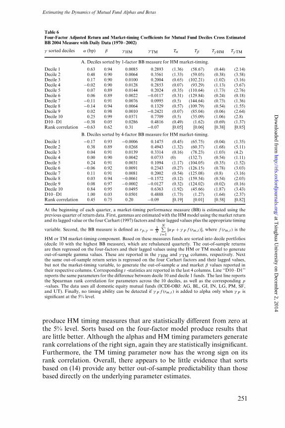
where f (rm,t ) is the HM or TM market-timing component as defined infootnote 5. This measure has the advantage of using the model’s overallreturn forecast as the benchmark rather than the accuracy of the individ-ual parameters. Thus, if the model’s estimation errors tend to cancel out,Equation (14) may reveal an as yet undetected forecasting power. Table 6examines this possibility using daily data because one might hope that theHM or TM models will produce their best estimates in this case.18

To create Table 6, parameters are estimated quarterly and the portfoliosrebalanced accordingly. The data is then sorted on the basis of thein-sample estimate of Equation (14). Panel A provides results from theone-factor model. As the α and γ TM columns show, sorting on (14) in-sample then leads to out-of-sample sorts on these two parameters that arein inverse order. Though the rank correlation coefficient on the HM timingmeasure has the right sign, it is not significant. Also, none of the deciles

18 The same tests reported in Table 6 were also conducted with monthly data. Because the conclusions tobe drawn from the monthly data are similar to those from the daily data, they are not reported here.Interested readers can obtain a copy of the table from the authors.

18


250

at Tsinghua U

niversity on Decem


Dow

nloaded from



Table 6Four-Factor Adjusted Return and Market-timing Coefficients for Mutual Fund Deciles Cross EstimatedBB 2004 Measure with Daily Data (1970–2002)

γ sorted deciles α (bp) β γ HM γ TM Tα Tβ Tγ HM Tγ TM

A. Deciles sorted by 1-factor BB measure for HM market-timing.

Decile 1 0.63 0.94 0.0085 0.2893 (1.36) (58.67) (0.44) (2.14)

Decile 2 0.48 0.90 0.0064 0.3561 (1.33) (59.05) (0.38) (3.58)

Decile 3 0.17 0.90 0.0100 0.2004 (0.65) (102.21) (1.02) (3.16)

Decile 4 −0.02 0.90 0.0128 0.2853 (0.07) (93.29) (1.13) (3.67)

Decile 5 0.07 0.89 0.0144 0.2024 (0.35) (110.64) (1.73) (2.76)

Decile 6 0.06 0.89 0.0022 −0.0117 (0.31) (129.84) (0.24) (0.18)

Decile 7 −0.11 0.91 0.0076 0.0995 (0.5) (144.64) (0.73) (1.36)

Decile 8 −0.14 0.94 0.0064 0.1329 (0.57) (109.79) (0.54) (1.55)

Decile 9 0.02 0.98 0.0010 −0.2421 (0.07) (85.04) (0.06) (2.64)

Decile 10 0.25 0.99 0.0371 0.7709 (0.5) (35.09) (1.06) (2.8)

D10–D1 −0.38 0.05 0.0286 0.4816 (0.49) (1.62) (0.69) (1.37)

Rank correlation −0.63 0.62 0.31 −0.07 [0.05] [0.06] [0.38] [0.85]

B. Deciles sorted by 4-factor BB measure for HM market-timing.

Decile 1 −0.17 0.93 −0.0006 0.1475 (0.45) (65.75) (0.04) (1.35)

Decile 2 0.38 0.89 0.0268 0.4943 (1.32) (60.37) (1.68) (5.11)

Decile 3 0.04 0.91 0.0139 0.3314 (0.16) (78.23) (1.03) (4.2)

Decile 4 0.00 0.90 0.0042 0.0733 (0) (132.7) (0.54) (1.11)

Decile 5 0.24 0.91 0.0031 0.1094 (1.17) (104.05) (0.35) (1.52)

Decile 6 −0.06 0.92 0.0091 0.2343 (0.27) (126.15) (0.78) (3.03)

Decile 7 0.11 0.91 0.0081 0.2002 (0.54) (125.08) (0.8) (3.16)

Decile 8 0.03 0.94 −0.0061 −0.1572 (0.12) (159.54) (0.54) (2.03)

Decile 9 0.08 0.97 −0.0002 −0.0127 (0.32) (124.02) (0.02) (0.16)

Decile 10 0.84 0.95 0.0495 0.6363 (1.92) (45.66) (1.87) (3.43)

D10–D1 1.00 0.03 0.0501 0.4888 (1.73) (1.27) (1.64) (2.37)

Rank correlation 0.45 0.75 0.20 −0.09 [0.19] [0.01] [0.58] [0.82]

At the beginning of each quarter, a market-timing performance measure (BB) is estimated using theprevious quarter of return data. First, gammas are estimated with the HM model using the market returnand its lagged value or the four Carhart (1997) factors and their lagged values plus the appropriate timing

variable. Second, the BB measure is defined as rp,γ = 1N

N∑t=1

[αP + γ P f (rm,t )], where f (rm,t ) is the

HM or TM market-timing component. Based on these measures funds are sorted into decile portfolios(decile 10 with the highest BB measure), which are rebalanced quarterly. The out-of-sample returnsare then regressed on the four-factors and their lagged values using the HM or TM model to generateout-of-sample gamma values. These are reported in the γ HM and γ TM columns, respectively. Nextthe same out-of-sample return series is regressed on the four Carhart factors and their lagged values,but not the market-timing variable, to generate the out-of-sample α and market β values reported intheir respective columns. Corresponding t -statistics are reported in the last 4 columns. Line ‘‘D10–D1’’reports the same parameters for the difference between decile 10 and decile 1 funds. The last line reportsthe Spearman rank correlation for parameters across the 10 deciles, as well as the corresponding p

-values. The data uses all domestic equity mutual funds (ICDI-OBJ: AG, BL, GI, IN, LG, PM, SF,and UT). Finally, no timing ability can be detected if γP f (rm,t ) is added to alpha only when γP issignificant at the 5% level.

produce HM timing measures that are statistically different from zero atthe 5% level. Sorts based on the four-factor model produce results thatare little better. Although the alphas and HM timing parameters generaterank correlations of the right sign, again they are statistically insignificant.Furthermore, the TM timing parameter now has the wrong sign on itsrank correlation. Overall, there appears to be little evidence that sortsbased on (14) provide any better out-of-sample predictability than thosebased directly on the underlying parameter estimates.

19251

at Tsinghua U

niversity on Decem


Dow

nloaded from



Comparing Table 5 to Table 6, one can see the difference in the out-of-sample performance of the Kalman filter HM models. Unlike the HMmodel, in-sample sorts based on the Kalman model’s market-timing mea-sure sort the funds out-of-sample by their HM and TM timing parametersas well. From a practical standpoint, the Kalman filter results are alsoeasier to utilize. Investors wishing to use the results in Table 6 need torebalance their portfolio every quarter, which can yield large tax bills andother transactions costs. In contrast, the numbers in Table 5 use monthlydata with portfolios that are rebalanced annually. This makes it mucheasier to exploit any of the Kalman model’s results that an investor maywish to take advantage of.

4.2 A general omnibus parameter testSome of the results presented in Section 3 indicate that the statisticalmodels may balance errors in one variable against those in another. Inthe case of the TM and HM models this may account for the negativecorrelation between the alpha and gamma estimates. Thus, the only way tojudge a model’s overall fit is to control for all of its estimated parameterssimultaneously and then examine the resulting portfolio’s sample statistics.

To create omnibus out-of-sample tests, this article proposes a three-stepprocess. First, each model is estimated fund by fund. Second, using theestimated parameters a portfolio with a forecasted zero alpha, zero beta,and (where appropriate) zero gamma is created. This is done by goinglong the fund, taking countervailing positions in the underlying factors,and then subtracting the predicted alpha value. By repeating the aboveprocedure, a time series of returns is produced (1970–2002 for this article’sdata set). Third, the resulting return sequence is then regressed against theappropriate factor model. A model without any forecasting error shouldproduce portfolios that yield excess returns (alphas) and factor loadings(betas and gammas) of exactly zero. Positive regression parameters indi-cate that a model has underestimated a value, while negative regressionparameters imply the opposite.

For the omnibus test described, eight models are tested: the OLS,Kalman, TM, and HM models in both their one- and four-factor forms. Ineach test the same model is used for all three steps. Thus, if the one-factorOLS model is used to create the portfolio (steps one and two), then the one-factor OLS model is used to determine the out-of-sample distribution of theportfolio’s loadings (step three). The only exceptions are the Kalman filtermodels. The one-factor Kalman filter model is tested out of sample withthe one-factor OLS model. Similarly, the four-factor Kalman filter modelis paired with the four-factor OLS model. This asymmetric treatmentof the Kalman filter models derives from the theoretical properties thatan out-of-sample portfolio should possess if the model that created it isproperly specified. With a properly specified model the first two steps

20


252

at Tsinghua U

niversity on Decem


Dow

nloaded from



should generate portfolio returns that have time-invariant parametersequal to zero. A static OLS model should thus be the ideal instrument withwhich to capture or reject this hypothesis.

Why not use the TM and HM models for the out-of-sample Kalmantests? If the TM and HM models properly describe the data-generationprocess, then there is no harm in using them. In such cases the out-of-sample portfolio returns they produce should have constant zero-valuedparameters, and the step-three model estimates should reflect this. Thus,the use of the TM and HM models for their own step-three testing is bothlogically consistent and has the advantage of producing a bootstrappeddistribution for the out-of-sample market-timing parameter (γ ). Asdiscussed earlier, however, these two models tend to produce nonzerogammas at too high a rate even when there is every reason to believethat the portfolios in question have zero gammas. Once the TM and HMmodels no longer form the null hypothesis, there is no reason to believe thattheir out-of-sample step three estimates will be unbiased. Thus, using themin step three to test whether the OLS or Kalman models have correctlyhedged out each fund’s market-timing ability is problematic.19

Table 7 reports the distributions from the three-step omnibus testsproposed above. Portfolio returns are bootstrapped with replacement1000 times. The forecast errors are also broken down by fund turnover. Asnoted earlier, it seems intuitive that the OLS models should do better whenfund turnover is low, and the Kalman filter model when it is high. Unlikethe previous set of tables, Table 7 also includes OLS models without thegamma timing parameter. This was done to see if the timing parameteractually helps or hinders the estimation of the other factors.

Each panel in Table 7 includes three sets of parameter statistics. The firstis the alpha error, the second the ‘‘return-weighted beta error,’’ and thethird the gamma error for the HM and TM models. The alpha and gammaerrors are simply the estimated alphas and gammas of the supposedlyzero-alpha, zero-beta, and zero-gamma portfolios. The return-weightedbeta is a variable designed to capture the overall misestimate of the factorloadings within a single statistic. It is constructed by multiplying thefactor loadings estimated on the out-of-sample predicted zero-alpha andzero-beta (and zero gamma for the HM and TM models) returns by eachfactor’s average value over the sample period and adding the productstogether:

return weighted beta error ≡∑

i

βi r i . (15)

19 For the Kalman filter model it is also somewhat unnecessary. The Kalman filter model attempts to forecastthe time-varying factor loadings. Assuming it is successful then, by construction, the step-two fund returnsshould lack any market-timing ability.

21253

at Tsinghua U

niversity on Decem


Dow

nloaded from



Table 7Out-of-Sample Returns for Zero-Alpha and Zero-Beta Portfolios

mean std 5% 10% 50% 90% 95%

Panel A: Results for the 1/3 of all funds with the lowest turnover ratio.Alpha error

OLS 1F 3.35 1.68 0.68 1.20 3.30 5.47 6.19

OLS 4F −2.70 1.17 −4.62 −4.27 −2.71 −1.20 −0.86

HM 1F 5.16 2.69 0.78 1.68 5.06 8.60 9.49

HM 4F −8.99 1.89 −12.24 −11.35 −9.03 −6.64 −5.90

TM 1F 9.29 2.57 5.09 6.08 9.28 12.75 13.54

TM 4F −3.82 1.46 −6.15 −5.62 −3.86 −1.95 −1.45

KAL 1F 1.20 1.88 −2.01 −1.33 1.26 3.55 4.15

KAL 4F −6.02 2.04 −9.50 −8.49 −6.09 −3.40 −2.61Return weighted beta error (bp)

OLS 1F 0.02 0.21 −0.33 −0.24 0.02 0.28 0.36

OLS 4F 2.70 0.55 1.81 2.00 2.73 3.39 3.57

HM 1F −1.12 0.35 −1.70 −1.57 −1.11 −0.68 −0.57

HM 4F 1.24 0.65 0.17 0.46 1.24 2.08 2.29

TM 1F 1.07 0.44 0.39 0.50 1.07 1.64 1.80

TM 4F 2.88 0.57 1.93 2.16 2.88 3.57 3.84

KAL 1F −0.11 0.25 −0.54 −0.43 −0.11 0.22 0.30

KAL 4F 1.91 0.83 0.55 0.87 1.91 2.96 3.19Gamma error

HM 1F −0.01 0.01 −0.02 −0.02 −0.01 0.00 0.01

HM 4F 0.04 0.01 0.02 0.03 0.04 0.05 0.05

TM 1F −0.10 0.04 −0.16 −0.14 −0.10 −0.05 −0.04

TM 4F 0.04 0.03 −0.01 0.00 0.04 0.08 0.09

Panel B: Results for the 1/3 of all funds with middle turnover ratio.Alpha error

OLS 1F 1.37 1.49 −1.14 −0.57 1.34 3.29 3.80

OLS 4F −4.42 1.25 −6.46 −6.03 −4.46 −2.80 −2.27

HM 1F 9.28 2.89 4.70 5.76 9.14 12.94 14.13

HM 4F −5.38 2.26 −9.02 −8.19 −5.37 −2.56 −1.54

TM 1F 11.11 2.53 6.95 7.83 11.11 14.36 15.23

TM 4F −1.64 1.50 −4.28 −3.61 −1.61 0.21 0.78

KAL 1F −2.64 1.77 −5.60 −4.98 −2.57 −0.42 0.26

KAL 4F −4.74 1.72 −7.49 −6.89 −4.78 −2.57 −1.96Return weighted beta error (bp)

OLS 1F 0.05 0.25 −0.34 −0.25 0.04 0.37 0.48

OLS 4F −0.59 0.69 −1.74 −1.45 −0.59 0.34 0.56

HM 1F −1.33 0.44 −2.08 −1.90 −1.33 −0.76 −0.61

HM 4F −0.87 0.82 −2.27 −1.95 −0.83 0.17 0.44

TM 1F 0.27 0.41 −0.43 −0.27 0.27 0.78 0.91

TM 4F −0.54 0.65 −1.60 −1.39 −0.54 0.24 0.53

KAL 1F 0.09 0.28 −0.38 −0.27 0.09 0.44 0.55

KAL 4F −2.19 0.81 −3.48 −3.24 −2.19 −1.15 −0.88

22


254

at Tsinghua U

niversity on Decem


Dow

nloaded from



Table 7(Continued)

mean std 5% 10% 50% 90% 95%

Gamma error

HM 1F −0.02 0.01 −0.03 −0.03 −0.02 0.00 0.00

HM 4F 0.03 0.01 0.02 0.02 0.03 0.05 0.05

TM 1F −0.18 0.05 −0.25 −0.23 −0.18 −0.12 −0.10

TM 4F −0.01 0.04 −0.08 −0.07 −0.02 0.04 0.05Panel C: Results for the 1/3 funds of all funds with the highest turnover ratio.

Alpha error

OLS 1F 11.78 2.28 8.17 8.92 11.75 14.74 15.43

OLS 4F −4.22 1.45 −6.65 −6.08 −4.26 −2.39 −1.82

HM 1F 15.87 3.00 11.06 12.05 15.72 19.72 20.78

HM 4F −2.27 2.47 −6.18 −5.34 −2.34 0.84 1.71

TM 1F 14.67 2.64 10.53 11.22 14.47 18.23 19.16

TM 4F −2.16 1.63 −4.81 −4.29 −2.12 −0.06 0.45

KAL 1F −2.68 3.05 −7.94 −6.63 −2.58 1.18 2.18

KAL 4F 1.64 2.34 −2.11 −1.44 1.72 4.59 5.58Return weighted beta error (bp)

OLS 1F −0.99 0.38 −1.63 −1.48 −0.98 −0.50 −0.40

OLS 4F −1.13 0.79 −2.45 −2.19 −1.13 −0.09 0.19

HM 1F −0.46 0.57 −1.38 −1.18 −0.48 0.23 0.52

HM 4F −2.03 0.99 −3.65 −3.31 −2.05 −0.78 −0.36

TM 1F 1.33 0.49 0.52 0.73 1.30 1.96 2.21

TM 4F −1.39 0.82 −2.81 −2.45 −1.38 −0.34 −0.05

KAL 1F −0.55 0.41 −1.23 −1.05 −0.54 −0.03 0.13

KAL 4F −3.46 0.97 −5.06 −4.73 −3.47 −2.22 −1.86Gamma error

HM 1F −0.02 0.01 −0.04 −0.03 −0.02 −0.01 0.00

HM 4F 0.06 0.01 0.04 0.05 0.07 0.08 0.08

TM 1F −0.20 0.06 −0.29 −0.27 −0.19 −0.12 −0.10

TM 4F 0.13 0.06 0.01 0.05 0.13 0.21 0.22

For all domestic equity mutual funds (ICDI-OBJ: AG, BL, GI, IN, LG, PM, SF, and UT) that had atleast five years of monthly return data, both 1-factor and 4-factor OLS, TM, HM, and Kalman modelsare used to forecast a fund’s alpha and beta (and for the HM and TM models gamma) at the beginningof each year from 1970 to 2002. These forecasts are then used to construct fund-by-fund zero-alphaand zero-beta (and if appropriate zero gamma) portfolios. Next, the resulting monthly time series forthe zero-alpha and zero-beta portfolio is regressed against the market factor (for one-factor models),the four factors (for four-factor models), or the corresponding factors plus market-timing component(for HM and TM models). This process results in risk-adjusted returns (the alpha error) and factorloadings for each zero-alpha zero-beta portfolio. A gamma error is also produced when zero-alpha,zero-beta, and zero-gamma portfolios are produced. The parameter distributions are then calculatedby bootstrapping with replacement the above procedure 1,000 times. The return-weighted beta error isdefined as: return-weighted beta error ≡ ∑

i βi ri , where βi is the estimated value of factor i, and ri thefactor’s average return during the sample period. The Kolmogorov–Smirnov test rejects the hypothesisthat the same probability distribution produced any pair of distributions generated by the differentmodels (all p -values virtually zero).

23255

at Tsinghua U

niversity on Decem


Dow

nloaded from



In this equation βi is the estimated loading of factor i from theregression, and ri the factor’s average return during the sample period.This metric is designed to give greater weight to those factors, which, ifmisestimated, will yield the largest systematic errors regarding a fund’spredicted performance. The closer a model comes to producing return-weighted beta errors of zero, the better it is at predicting a fund’s overallfuture factor risks and returns.

Table 7 Panel A displays the results for low-turnover funds. Assumingthat most stock betas remain fairly constant over time, these funds wouldseem to be ideally suited for OLS models as they are the most likelyto have either static or slowly changing factor loadings. For the out-of-sample alpha errors only the one-factor Kalman model encompasseszero within the 90% confidence interval. By contrast, the four-factor OLSmodel produces portfolio returns with a 90% confidence of −4.62 bps(basis points) to −0.86 bps per month, indicating that it overpredictsfund alphas. The four-factor HM and TM models also produce portfolioreturns that are strictly negative (implying they too overpredict the alphas)throughout the 90% confidence interval. Thus, if the goal is to produce anunbiased forecast of a fund’s alpha, the one-factor Kalman model appearsto provide the best performance.

The middle part of Table 7 Panel A reports the bootstrapped distributionof the return-weighted beta error. Once again only the one-factor Kalmanmodels include zero within the 90% confidence interval.

The final section of the panel displays the results for the gamma errors.Here at least the one-factor HM and four-factor TM models encompasszero within the 90% confidence interval. However, it is worth noting thatof all the funds these are the most likely to display the least market-timingability, and two of the four models still fail to produce forecast errorsaround zero a reasonable fraction of the time.

Table 7 Panel B examines funds with turnover ratios in the middlethird of the data and Panel C the funds with the highest turnover ratios.These are the groups that are more likely to create problems for theOLS models, and the ones that the TM and HM models attempt toaddress. However, the results do not provide much support for the latter.Of the models tested, only the one-factor Kalman model encompasseszero within the 90% confidence interval for both the out-of-sample alphaand return-weighted beta. The one-factor OLS model manages to do thesame, but only for the middle-turnover group. The four-factor TM modelcomes close, failing to encompass zero only for the high-turnover group’sreturn-weighted beta. However, the gamma error for this group does notcover zero, which is troubling, because that is the parameter on whichmost applications of this model concentrate.

Overall, three panels of Table 7 indicate that the one-factor Kalmanmodel produces in-sample parameter estimates that successfully forecast

24


256

at Tsinghua U

niversity on Decem


Dow

nloaded from



a fund’s future factor loadings. The other models are far less accurate onthis front. Oddly, the OLS models appear to do particularly poorly withlow-turnover ratio funds: the one group the model should be best adaptedto. A natural conclusion is that even low-turnover funds have sufficientlydynamic factor loadings that the OLS models end up producing biasedforecasts.

5. Time Variation in Mutual Fund Betas

Although the Kalman filter’s parameter estimates have a number ofdesirable properties, are they economically reasonable? Mutual fundscannot change their portfolio holdings very quickly, so their estimatedfactor loadings should not vary too much or too fast. Figure 1 providessome intuition regarding the actual time variation in fund factor loadingsand the Kalman filter model’s ability to track the observed changes. Thisfigure has three panels, each of which presents a set of comparative graphsfor a representative fund by turnover group.

The first fund in Figure 1 is ICDI 660. It has a low annual turnover of0.38. Not too surprisingly, it also has fairly time-invariant factor loadings.The green lines represent the rolling OLS estimates and the blue linesthe Kalman filter estimates. First, note that while a σβ,CAPM of 0.12 mayappear to be high, it actually produces a relatively stable time series. Theother thing to note is that the rolling OLS and Kalman filter estimatestrack each other fairly well, although not perfectly. In general, the Kalmanfilter estimates appear smoother and less prone to sudden shifts. Giventhe out-of-sample evidence presented earlier, it seems likely that the sharpfluctuations in the OLS parameter estimates are due to estimation errorsof some sort and not real changes in the fund’s holdings.

The next set of graphs examine fund ICDI 14 670. It has an averageturnover level of 0.69. Here, σβ,CAPM equals 0.16, but neverthelessthe model produces a factor-loading time series that slowly increasesthroughout the 1990s. Again the model has several interacting variables,and simply looking at the implied variance of the market factor fails to tellthe whole story. Also note that here, too, the Kalman filter estimates areat least as smooth as the rolling OLS estimates. For example, the Kalmanfilter model finds that the fund’s estimated alpha is near zero throughoutmost years except for a few short negative periods. In contrast, the OLSmodel claims that the fund’s alpha has varied dramatically from year toyear, a feat that seems highly unlikely given what we know about theforecasting power typically associated with such models.

The third panel in Figure 1 looks at fund (ICDI 8100), which has ahigh turnover ratio of 1.22. The comparative results between the OLS andKalman models are qualitatively similar to those in the other two panels.Here, though, both models indicate that the fund’s factor loadings have

25257

at Tsinghua U

niversity on Decem


Dow

nloaded from



1970 1980 1990 20000

0.5

1B1. Beta (ICDI = 660)

1975 1985 1995–5

0

5x 10–3 A2. Alpha (ICDI = 14670)

1975 1985 19950

0.5

1

1.5B2. Beta (ICDI = 14670)

1970 1980 1990 2000–0.02

–0.01

0

0.01

0.02A3. Alpha (ICDI = 8100)

1970 1980 1990 20000.5

1

1.5

2B3. Beta (ICDI = 8100)

1970 1980 1990 2000–0.01

0

0.01

0.02A1. Alpha (ICDI = 660)

KalOLS60

Fund ICDI Turnover

660 0.12 0.0514670 0.16 0.12

8100 0.23 0.21

0.380.691.22

σβ,CAPM σβ,FF

Figure 1Time series of Kalman model estimated mutual fund alphas and betas.First, Kalman one- and four-factor models are used to estimate the time series of mutual fund alphas andbetas based on available monthly return data in the period from 1970 to 2002. The blue lines plot theestimated time series for one-factor alpha and beta (for the one-factor Kalman model in Panels A and B)for three mutual funds with low, medium, and high turnover ratios. To save space, four-factor exposuresand risk-adjusted returns are not plotted. Green lines plot the rolling OLS values of the correspondingparameter. The OLS alpha and beta values in month t are estimated from month t − 60 to month t − 1.Fund information is summarized in the table.

varied quite a bit over the years. However, once again the OLS valuesoften tend to fluctuate more than the Kalman filter estimates, especially inregard to the nonmarket factors SMB, HML, and MOM.

Although Figure 1 provides some insight regarding the volatility ofthe Kalman filter estimates, Table 8 examines the issue more broadly.In this table the Kalman model’s parameter estimates are brokendown by fund turnover and the factor model used. The penultimatecolumn in each panel displays the average estimated time variationin the fund betas for each turnover group (σβ ), and the last columnprovides the variance of the residual from fitting an AR(1) to eachfund’s beta over time. The former measure yields the total variation,

26


258

at Tsinghua U

niversity on Decem


Dow

nloaded from



Tab

le8

Ave

rage

Cro

ss-S

ecti

onal

Kal

man

Par

amet

erS

tati

stic

s

A.K

alm

anpa

ram

eter

sfo

r1-

fact

ordy

nam

icm

odel

Tur

nove

r−k

βp

υσ

εσ

2 ηα

pb P

σβ

σβ,A

R(1

)

Low

0.00

070.

7825

0.57

470.

0224

0.04

91−0

.000

4−0

.268

60.

1375

0.12

84M

edia

−0.0

004

0.88

250.

5815

0.02

240.

0627

0.00

06−0

.127

20.

1529

0.14

07H

igh

−0.0

011.

0393

0.54

30.

0265

0.10

290.

0226

0.17

090.

1787

0.16

04T

-sta

tL

ow(4

.87)

(94.

23)

(72.

48)

(20.

53)

(20.

15)

(0.0

8)(7

.26)

(61.

46)

(32.

86)

Med

ia(1

.21)

(98.

04)

(75.

50)

(27.

65)

(18.

54)

(0.1

3)(3

.06)

(64.

59)

(31.

76)

Hig

h(4

.57)

(92.

17)

(70.

45)

(30.

92)

(19.

03)

(6.2

1)(3

.90)

(64.

64)

(41.

59)

B.K

alm

anpa

ram

eter

sfo

r4-

fact

ordy

nam

icm

odel

Tur

nove

r−k

βM

KT

βS

MB

βH

ML

βM

OM

υσ

εσ

2 ηc S

MB

c HM

Lc M

OM

αp

b Pσ

βσ

β,A

R(1

)

Low

−0.0

006

0.86

670.

096

0.14

6−0

.025

30.

5513

0.01

410.

0501

0.11

53−0

.258

8−0

.051

6−0

.008

50.

0857

0.12

850.

1038

Med

ia−0

.001

40.

9257

0.18

240.

0804

0.00

940.

5925

0.01

410.

0545

−0.0

823

−0.1

336

0.12

90.

0032

0.08

990.

1407

0.11

01H

igh

−0.0

019

0.97

230.

2832

−0.0

828

0.06

220.

5907

0.01

730.

0515

−0.1

454

−0.8

213

0.21

650.

0137

0.10

160.

1602

0.12

7T

-sta

tL

ow(4

.19)

(142

.93)

(10.

29)

(9.8

7)(7

.94)

(58.

90)

(11.

91)

(10.

78)

(0.9

7)(1

.59)

(0.5

6)(1

.24)

(1.7

3)(3

2.88

)(2

3.97

)

Med

ia(6

.74)

(148

.89)

(15.

85)

(7.6

8)(2

.10)

(64.

60)

(17.

69)

(9.4

8)(0

.67)

(0.8

3)(1

.01)

(0.4

2)(1

.94)

(31.

76)

(23.

03)

Hig

h(5

.04)

(122

.13)

(25.

94)

(6.4

4)(9

.49)

(68.

15)

(25.

60)

(15.

44)

(1.2

4)(5

.43)

(1.7

6)(1

.79)

(2.0

3)(4

1.59

)(2

8.51

)

Thi

sta

ble

repo

rts

the

esti

mat

edK

alm

anpa

ram

eter

sfo

ra

one-

and

four

-fac

tor

mod

el.T

heK

alm

anpa

ram

eter

sar

ees

tim

ated

base

don

mon

thly

retu

rnda

tafr

om19

70to

2002

.M

utua

lfu

nds

are

sort

edin

toth

ree

grou

psac

cord

ing

toth

eav

erag

etu

rnov

erra

tio

duri

ngth

esa

me

peri

od(t

hebr

eak

poin

tsoc

cur

atan

nual

turn

over

rate

sof

0.55

96an

d1.

0107

).E

ach

entr

yth

enre

port

sst

atis

tics

rega

rdin

gth

epa

ram

eter

valu

esw

ithi

nth

esa

me

turn

over

grou

p.T

hela

sttw

oco

lum

nsco

ntai

nth

est

anda

rdde

viat

ion

ofth

efu

nd’s

mar

ket

expo

sure

( σβ

)an

dth

atof

the

resi

dual

from

anA

R(1

)fit

ofth

efu

nd’s

mar

ket

expo

sure

(σβ,A

R(1

)).

The

cros

s-se

ctio

nt-

stat

isti

csar

ere

port

edin

pare

nthe

ses.

27259

at Tsinghua U

niversity on Decem


Dow

nloaded from



and the latter may be interpreted as the surprise in beta’s change fromperiod to period. As both columns indicate, an increase in fund turnoverincreases the estimated volatility of the fund’s market beta. This result alsoindicates that the conjecture given in footnote 9, that stock betas changeover time and that fund managers trade to maintain constant portfolioloadings, is not supported by the data.

Beyond the beta volatility figures, the other parameter estimates inTable 8 also seem to conform to expectations. For the middle-turnovergroups the persistence parameter υ is about 0.58 and the standard devia-tion of the signal’s innovation (σ 2

η) equals 0.0627. The combination of therelatively rapid revision of the fund’s beta to its long-run mean at a rate ofapproximately 45% per month and the signal’s relatively modest varianceimplies that though betas can drift somewhat from their long-run means,they do not do so for very long. This in turn leads to the relatively modestvalues observed in the σβ column.

6. Comparison with the FS Model

So far all tests have been conducted under the restriction that the fundbetas depend only upon some unobservable factor. This section examinesthe impact on the estimated model when observable conditioning infor-mation is added. The tests conducted here use the lagged Treasury-billrate and the dividend yield on the CRSP value-weighted index. Thus, theequation for βPt becomes

βPt = β + Ft−1 + k1z1,t−1 + k2z2,t−1. (16)

If the observable information improves the model’s predictive ability, thenk1 and k2 should differ from zero. This is tested by running the modelwith and without the conditioning variables on monthly returns duringthe period 1970–2002. Asymptotically, the likelihood ratio under the nullshould follow a chi-square distribution with two degrees of freedom.In Figure 2, the bars represent the cross-sectional distribution of thelikelihood ratio, and the dashed line traces out a chi-square distributionwith two degrees of freedom. Overall, the null hypothesis that k1 and k2are zero cannot be rejected at the traditional 1, 5, or 10% levels. However,for individual funds, the fraction that rejects the null hypothesis at the 1, 5,or 10% level is 10, 20, and 27%, respectively. These numbers are somewhathigher than might be expected by chance, which implies that for somefunds the conditioning information appears to improve the model’s fit.

Table 9 provides further evidence about the richness of the dynamiccoefficient model used in this article. This table shows the R2’s for thefund return regressions using the OLS, the FS two-factor conditional beta

28


260

at Tsinghua U

niversity on Decem


Dow

nloaded from



0 5 10 15 20 25 30 35 40 450

0.1

0.2

0.3

0.4

0.5

Likelihood Ratio: 10%, 20%, and 27% of funds rejectthe null at the 1%, 5%, and 10% level

Likelihood Ratio Test for Conditional Beta Model: Lagged TBill and Dividend–Ratio

Chi2 PDF with 2 degrees of freedomPDF for likelihood ratio

Figure 2Likelihood ratio tests.This figure shows the results from a likelihood ratio test in which the Kalman filter model includesconditional information similar to that of Ferson and Schadt (1996). As in their application, laggedmacroeconomic information drives the portfolio weights. However, here portfolio weights are alsoassumed to vary from some unobserved factor following an AR(1) process. As a first-order approximationthe portfolio weights are set to wit = wi + liFt + DiZt−1, where Zt−1 is the lagged information. This modelis estimated via an extended Kalman filter. For two macro instruments, the estimated system of equations isgiven by rPt − rft = αPt + βPt(rmt − rft) + βX,tXt + εPt, where βPt = βP + Ft−1 + k1z1,t−1 + k2z2,t−1

and αPt = −kt + αP Ft−1 + bP F 2t−1, Ft = νFt−1 + ηt , and Xt are other factors (SMB, HML, and MOM).

Here z1 and z2 are instruments for the lagged treasury-bill rate and the CRSP value-weighted index’sdividend yield. The null hypothesis is that k1 = k2 = 0. The constrained and unconstrained models areestimated using available monthly returns of CRSP equity mutual funds during the period of 1970 to 2002(a minimum of 60 monthly returns are required). Asymptotically, the likelihood ratio test under the nullshould follow a chi-square distribution with two degrees of freedom. The bars represent the cross-sectionaldistribution of the likelihood ratio and the dashed line displays the mathematical values for a chi-squaredistribution with two degrees of freedom. The fraction of funds that reject the null hypothesis at the 1, 5,or 10% levels are 10, 20, and 27%, respectively.

model, and this article’s Kalman filter model across turnover terciles.20 Ascan be seen, for each tercile and for the entire sample the FS model providesan improved fit relative to the OLS model (the differences are all statisticallysignificant). Consider, however, how the R2 statistic changes as one movesacross models. The increase when one goes from the OLS to FS model is lessthan 10% of the increase obtained when moving from the FS to the Kalmanmodel. On the basis of this, it appears that the Kalman model can accountfor a considerably larger portion of fund return fluctuations than either

20 The Kalman model used in these tests does not use the FS conditioning variables and looks only at thereturn series of funds and the market index.

29261

at Tsinghua U

niversity on Decem


Dow

nloaded from



Table 9A Comparison with Conditional Model

Turnover R2CAPM R2

Cond R2Kal �R2

1 �R22 T

�R21

T�R2

2

Panel A: 1-factor modelLow 0.7120 0.7326 0.8713 0.0206 0.1387 (31.28) (40.86)

Media 0.7007 0.7211 0.8683 0.0204 0.1472 (30.85) (42.01)

High 0.6954 0.7165 0.8769 0.0211 0.1604 (25.90) (44.73)

All 0.7027 0.7234 0.8722 0.0207 0.1488 (50.18) (73.59)

Panel B: 4-factor modelLow 0.8317 0.8426 0.9478 0.0109 0.1053 (30.40) (33.84)

Media 0.8322 0.8431 0.9498 0.0109 0.1067 (28.49) (33.18)

High 0.8271 0.8395 0.9517 0.0124 0.1122 (22.34) (37.39)

All 0.8303 0.8417 0.9498 0.0114 0.1081 (44.76) (60.19)

The sample used for this table includes all equity mutual funds in the CRSP databasethat contain at least 60 months of monthly return data from 1970 to 2002. Modelparameters are estimated for the unconditional CAPM model, the conditional betamodel, and the Kalman filter model. The variables R2

CAPM, R2Cond, and R2

Kal represent

R2 statistics for each of the models, respectively. Consistent with the OLS model, R2Kal

is defined as 1 − E(εP (t)2)/E((yt − y)2), where yt is the excess portfolio return andεP (t)is the residual from the Kalman filter model. The variable y equals the mean valueof the yt . Also reported are the cross-sectional means and t -ratios for the improvementsof the R2 statistic: �R2

1 = R2Cond − R2

CAPM, and �R22 = R2

Kal − R2cond.

the OLS or the FS models. Also, as expected, the greatest improvementsrelative to the OLS model are for those funds that have the highest turnoverrates, and are thus likely to have the most dynamic factor loadings.

Between this article, FS, and Grinblatt and Titman (1989) there isnow considerable evidence that mutual fund managers produce portfolioswith time-varying betas, and possibly alphas, too. Thus, it is clear thatportfolio managers are altering their portfolios in response to some set ofeconomic variables. Why then are k1 and k2 statistically indistinguishablefrom zero for most funds? The model has two ways of fitting a fund’salphas and betas. One way is to use the observable conditioning variablesin some manner. Another is to use the estimated lagged values of alpha andbeta, and let them change according to an estimated relationship with anunobserved factor following an AR(1) process. Figure 2 indicates that thelatter prediction method often dominates, at least when using the laggedTreasury-bill rate and dividend yield on the CRSP value-weighted index.One conclusion may be that a few funds use Treasury-bill rates and themarket dividend yield to help manage their assets, though most do not.More practically, one can use the model to identify both those funds witha more macro-based approach to asset allocation and the variables onwhich they concentrate.

7. Conclusion

Mutual fund managers often trade in the hope of generating superiorreturns. This trading naturally generates time-varying factor loadings.

30


262

at Tsinghua U

niversity on Decem


Dow

nloaded from



However, the standard multifactor OLS is not designed to handle suchtime variation or to detect whether fund managers have the ability to timethe market by appropriately varying their fund’s beta. Potential solutionsto this problem are the TM and HM models, which include a market-timingparameter in addition to the standard factors. Using these models, BB findthat while there is no evidence that fund managers possess market-timingability in the monthly data, they are able to detect it in the daily data.

In line with BB this article finds that the TM and HM models producefalse-positive parameters with daily data at an extraordinarily high rate.However, the analysis here also indicates that the daily parameter estimatesare very unstable, with in-sample sorts leading to little out-of-samplepredictive power. To address the issue of time variation in mutual fundfactor loadings, this article develops a Kalman filter model. This modelgenerates dynamic factor loadings that can allow one to test for a fund’smarket-timing ability. Although the Kalman filter model does not appearto reliably find market-timing ability in the daily data, it does find suchability in the monthly data. Furthermore, the Kalman filter model’s timingability estimates in the monthly data exhibit good predictive power.

There are, of course, other dynamic models that have been proposed.The conditional model of FS is one example. Their conditional modeluses macroeconomic factors to help forecast a fund’s factor loadings. TheKalman filter model can accommodate the FS factors. However, testsindicate that for most funds the macroeconomic factors add little in theway of explanatory power.

ReferencesAdmati, A. 1985. A Noisy Rational Expectations Equilibrium for Multi-asset Securities Markets.Econometrica 53(3):629–57.

Ang, A., J. Chen, and Y. Xing. 2002. Downside Correlation and Expected Stock Returns,http://ssrn.com/abstract=282986, Accessed July 27, 2007.

Blake, D., B. Lehmann, and A. Timmermann. 1999. Asset Allocation Dynamics and Pension FundPerformance. Journal of Business 72(4):429–61.

Blake, D., B. Lehmann, and A. Timmermann. 2002. Performance Clustering and Incentives in the UKPension Fund Industry. Journal of Asset Management 3(2):173–94.

Bollen, N., and J. Busse. 2001. On the Timing Ability of Mutual Fund Managers. Journal of Finance56(3):1075–94.

Bollen, N., and J. Busse. 2005. Short-Term Persistence in Mutual Fund Performance. Review of FinancialStudies 18(2):569–97.

Brown, S., and W. Goetzmann. 1995. Performance Persistence. Journal of Finance 50(2):679–98.

Brown, S., and W. Goetzmann. 1997. Mutual Fund Styles. Journal of Financial Economics 43(3):373–99.

Carhart, M. 1997. On Persistence in Mutual Fund Performance. Journal of Finance 52(1):57–82.

Christopherson, J., W. Ferson, and D. Glassman. 1998. Conditioning Manager Alphas on EconomicInformation: Another Look at the Persistence of Performance. Review of Financial Studies 11:111–42.

31263

at Tsinghua U

niversity on Decem


Dow

nloaded from



Cohen, R., J. Coval, and L. Pastor. 2005. Judging Fund Managers by the Company They Keep. Journalof Finance 60(3):1057–96.

Daniel, K., M. Grinblatt, S. Titman, and R. Wermers. 1997. Measuring Mutual Fund Performance withCharacteristic-Based Benchmarks. Journal of Finance 52(3):1035–58.

Ferson, W., and C. Harvey. 1991. The Variation of Economic Risk Premiums. Journal of Political Economy99:385–415.

Ferson, W., and C. Harvey. 1993. The Risk and Predictability of International Equity Returns. Review ofFinancial Studies 6:527–66.

Ferson, W., and R. Korajczyk. 1995. Do Arbitrage Pricing Models Explain the Predictability of StockReturns? Journal of Business 68(3):309–49.

Ferson, W., and R. Schadt. 1996. Measuring Fund Strategy and Performance in Changing EconomicConditions. Journal of Finance 51(2):425–62.

Ferson, W., and K. Khang. 2002. Conditional Performance Measurement Using Portfolio Weights:Evidence for Pension Funds. Journal of Financial Economics 65:249–82.

Grinblatt, M., and S. Titman. 1989. Portfolio Performance Evaluation: Old Issues and New Insights.Review of Financial Studies 2(3):396–422.

Grinblatt, M., and S. Titman. 1992. The Persistence of Mutual Fund Performance. Journal of Finance47(5):1977–84.

Grinblatt, M., and S. Titman. 1993. Performance Measurement Without Benchmarks: An Examinationof Mutual Fund Returns. Journal of Business 66(1):47–68.

Grinblatt, M., and S. Titman. 1994. A Study of Monthly Mutual Fund Returns and PerformanceEvaluation Techniques. Journal of Financial and Quantitative Analysis 29(3):419–44.

Harvey, A. 1989. Forecasting, Structural Time Series Models and the Kalman Filter. Cambridge: CambridgeUniversity Press.

Hendricks, D., J. Patel, and R. Zeckhauser. 1993. Hot Hands in Mutual Funds: Short-Run Persistence ofRelative Performance, 1974–1988. Journal of Finance 48(1):93–130.

Henriksson, R. D., and R. C. Merton. 1981. On Market-timing and Investment Performance. II. StatisticalProcedures for Evaluating Forecasting Skills. Journal of Business 54(4):513–33.

Jagannathan, R., and R. Korajczyk. 1986. Assessing the Market-timing Performance of ManagedPortfolios. Journal of Business 59(2):217–35.

Lehmann, B., and D. Modest. 1987. Mutual Fund Performance Evaluation: A Comparison of Benchmarksand Benchmark Comparisons. Journal of Finance 42:233–65.

Pastor, L., and R. Stambaugh. 2002. Mutual Fund Performance and Seemingly Unrelated Assets. Journalof Financial Economics 63(3):315–50.

Teo, M., and S. Woo. 2001. Persistence in Style-Adjusted Mutual Fund Returns. Working paper, HarvardUniversity, Department of Economics.

Treynor J. L., and K. Mazuy. 1966. Can Mutual Funds Outguess the Market? Harvard Business Review44:131–36.

Wermers, R. 2000. Mutual Fund Performance: An Empirical Decomposition into Stock-Picking Talent,Style, Transactions Costs, and Expenses. Journal of Finance 55(4):1655–95.

32


264

at Tsinghua U

niversity on Decem


Dow

nloaded from


Estimating the Dynamics of Mutual Fund Alphas … the... · Estimating the Dynamics of Mutual Fund...

Documents

Transcript of Estimating the Dynamics of Mutual Fund Alphas … the... · Estimating the Dynamics of Mutual Fund...