Estimating Probability of Blow Fly Colonization in Eastern ...

Western Washington UniversityWestern CEDAR

WWU Graduate School Collection WWU Graduate and Undergraduate Scholarship

Winter 2019

Estimating Probability of Blow Fly Colonization inEastern Washington: a Forensic EntomologyExperimentHeather Zarkos BoswellWestern Washington University, [email protected]

Follow this and additional works at: https://cedar.wwu.edu/wwuetPart of the Anthropology Commons

This Masters Thesis is brought to you for free and open access by the WWU Graduate and Undergraduate Scholarship at Western CEDAR. It has beenaccepted for inclusion in WWU Graduate School Collection by an authorized administrator of Western CEDAR. For more information, please [email protected].

Recommended CitationZarkos Boswell, Heather, "Estimating Probability of Blow Fly Colonization in Eastern Washington: a Forensic EntomologyExperiment" (2019). WWU Graduate School Collection. 854.https://cedar.wwu.edu/wwuet/854

https://cedar.wwu.edu/?utm_source=cedar.wwu.edu%2Fwwuet%2F854&utm_medium=PDF&utm_campaign=PDFCoverPages

https://cedar.wwu.edu/wwuet?utm_source=cedar.wwu.edu%2Fwwuet%2F854&utm_medium=PDF&utm_campaign=PDFCoverPages

https://cedar.wwu.edu/grad_ugrad_schol?utm_source=cedar.wwu.edu%2Fwwuet%2F854&utm_medium=PDF&utm_campaign=PDFCoverPages

https://cedar.wwu.edu/wwuet?utm_source=cedar.wwu.edu%2Fwwuet%2F854&utm_medium=PDF&utm_campaign=PDFCoverPages

http://network.bepress.com/hgg/discipline/318?utm_source=cedar.wwu.edu%2Fwwuet%2F854&utm_medium=PDF&utm_campaign=PDFCoverPages

https://cedar.wwu.edu/wwuet/854?utm_source=cedar.wwu.edu%2Fwwuet%2F854&utm_medium=PDF&utm_campaign=PDFCoverPages

mailto:[email protected]

Estimating Probability of Blow Fly Colonization

in Eastern Washington:

a Forensic Entomology Experiment

By

Heather Zarkos Boswell

Accepted in Partial Completion

Of the Requirements for the Degree

Master of Arts

ADVISORY COMMITTEE

Dr. Todd Koetje, Chair

Dr. Sarah Campbell

Dr. Kathleen Young

GRADUATE SCHOOL

Dr. Gautam Pillay, Dean

Master’s Thesis

In presenting this thesis in partial fulfillment of the requirements for a master’s thesis at

Western Washington University, I grant to Western Washington University the non-

exclusive royalty-free right to archive, reproduce, distribute, and display the thesis in any and

all forms, including electronic format, via any digital library mechanisms maintained by

WWU.

I represent and warrant this is my original work and does not infringe or violate any rights of

others. I warrant that I have obtained written permission from the owner of any third party

copyrighted material included in these files.

I acknowledge that I retain ownership rights to the copyright of this work, including but not

limited to the right to use all or part of this work in future works, such as articles or books.

Library users are granted permission for individual, research, and non-commercial

reproduction of this work for educational purposes only. Any further digital posting of this

document requires specific permission from the author.

Any copying or publication of this thesis for commercial purposes, or for financial gain, is

not allowed without my written permission.


Date:2/21/2019

Estimating Probability of Blow Fly Colonization

in Eastern Washington:

a Forensic Entomology Experiment

A Thesis

Presented to

The Faculty of

Western Washington University

In Partial Completion

Of the Requirements for the Degree

Master of Arts

By


March 2019

iv

Abstract

Accurately estimating the time since a decedent was alive (postmortem interval/PMI)

after the first 24 to 72 hours is dependent upon the ability of forensic entomologists to predict

the colonization of remains by insects. Estimations of PMI must be modified for local

conditions. This study examines the abiotic environmental factors (ambient temperature,

relative humidity, light intensity, rainfall, barometric pressure, and wind speed) that influence

the appearance of a specific subset of colonizing insects of forensic importance and known to

show up first in other North American settings. These insects include blow and bottle flies,

from the taxonomic family of Calliphoridae. The goal is to clarify the impact of abiotic

environmental factors on predicting the probability of colonization by blow flies in Eastern

Washington to more accurately estimate the postmortem interval (PMI). The hypothesis is

that ambient temperature, light intensity, and relative humidity will be the most significant

factors. About 1/3 to 1/2 of a pound of liver was placed in bowls protected by plastic cages

at three locations that differ in terms of the type of vegetation. Logistic regression utilizing

SPSS 25.0 (2017) generated equations of probability for blow fly colonization based on the

significant abiotic environmental variables. Results show that ambient temperature, relative

humidity, and light intensity are all significant predictor variables in blow fly colonization. In

addition to studies establishing equations for the probability of blow fly colonization in other

geographic regions, further studies are needed on the effects of wildfire smoke on blow fly

colonization and activity.

v

Acknowledgments

I would like to extend my gratitude to my thesis committee, Dr. Todd Koetje, Dr.

Sarah Campbell, and Dr. Kathleen Young, for their support and feedback during this process.

A special thank you goes to the late Dr. Joan Stevenson, who was instrumental in my choice

of forensic entomology as my thesis topic. In addition, I am also grateful to Dr. Sarah Keller

for her mentorship during my undergrad at Eastern Washington University.

A huge thank you goes to the hunters in my community who donated liver from their

harvested moose, deer, and elk for my research.

Thank you to my friends, family, my children, and especially my husband Kelly for

providing me with unfailing love and continuous encouragement throughout my years of

study and through the process of researching and writing this thesis. Thank you for helping

me follow my dreams!

For my mama, Melodi Coulson (1953-2018)

vi

Table of Contents

Abstract………………………………………………………………………………..……...iv

Acknowledgments…………………………………………..……………..…………………..v

List of Figures and Tables…………………………………………………………..……….vii

Chapter1: Introduction……………………...……………………………………………..… 1

Chapter 2: Estimating the Postmortem Interval ………………………………………………4

Chapter 3: Early Postmortem Events……………………..………..………………………….8

Chapter 4: Blow Fly Biology and Carrion Ecology…………………………………..……...11

Chapter 5: Methods…………..……………………………………………..…..……………20

Chapter 6: Climatic Conditions and Light Intensity.…………………………………..…….27

Chapter 7: Statistical Analysis of Calliphorid Colonization……………………………..….34

Chapter 8: Species Observed…………………………………………………………..…….68

Chapter 9: Unanticipated Confounding Factors………………………………………..……72

Chapter 10 Discussion and Conclusions………………………..……………………………79

Works Cited..……………………………………………………………………….....……..84

Appendix A……………………………………………………………..……………..…..…96

Appendix B……………………………………………………………..…..…………..……97

Appendix C……………………………………………………………..…..…………..……98

Appendix D……………………………………………………………..……………..……114

vii

List of Figures and Tables

Figure 1. Timeline of events in a death investigation……..………………………..…....……5

Table 1. Stages of Decomposition ………………………………….……………….......……8

Figure 2. Generalized blow fly life cycle…………………………………………….....……13

Table 2. Relevant studies…………………………………………….....……………...…….21

Figure 3a. Grass data collection site……………………………………………........………23

Figure 3b. Short tree data collection site…………………………………………….....……23

Figure 3c. Tall tree data collection site…………………………………………...….....……23

Figure 4. Colonization medium (liver) …………………………………………..….....……24

Figure 5. Evidence of blow fly colonization (egg masses) …………………………….....…25

Table 3. Descriptive stats colonization/temperature: experiment site………….............……27

Figure 6. Graph of temperature frequencies: experiment site……..………………...………27

Table 4. Descriptive stats colonization/relative humidity/rainfall: experiment site.………...28

Figure 7. Graph of relative humidity frequencies: experiment site…………....………….…29

Figure 8. Graph of rainfall frequencies: experiment site…………..…………………...……29

Table 5. Descriptive stats colonization/wind speed: experiment site…………..…..………..30

Figure 9. Graph of wind speed frequencies: experiment site………….…….…………..…..30

Table 6. Descriptive stats colonization/barometric pressure: experiment site………….……31

Figure 10. Graph of barometric pressure frequencies: experiment site………….....….….…31

Table 7. Light intensity levels for reference…………………………………………………32

Table 8. Descriptive statistics colonization/light intensity experiment site………….………32

Figure 11. Graph of light intensity frequencies: experiment site…………...………..………32

Table 9. The frequency of colonization for each habitat………………………...…………..33

Table 10. Collinearity diagnostics…………………………………………...………………35

Figure 12. Graph of collinearity diagnostics…………………………………………………35

Table 11. Correlation Statistics………………………………………………………………36

Figure 13a. Collinearity scatterplot: ambient temperature/light intensity………….…..……37

Figure 13b. Collinearity scatterplot: ambient temperature/relative humidity….……….……37

Figure 13c. Collinearity scatterplot: ambient temperature/ rainfall…………….……………37

Figure 13d. Collinearity scatterplot: ambient temperature/barometric pressure...............…..38

viii

Figure 13e. Collinearity scatterplot: ambient temperature/wind speed…………………...…38

Figure 14a. Collinearity scatterplot: relative humidity/light intensity……….…………..…..38

Figure 14b. Collinearity scatterplot: relative humidity/wind speed………………….………39

Figure 14c. Collinearity scatterplot: relative humidity/rainfall……………...………………39

Figure 14d. Collinearity scatterplot: relative humidity/barometric pressure…………...……39

Figure 15a. Collinearity scatterplot: light intensity/rainfall……………………….…………40

Figure 15b. Collinearity scatterplot: light intensity/wind speed…………………..…………40

Figure 15c. Collinearity scatterplot: light intensity/barometric pressure…………….………40

Figure 16a. Collinearity scatterplot: rainfall/wind speed………………………….…………41

Figure 16b. Collinearity scatterplot: rainfall/barometric pressure………...…………………41

Figure 17: Collinearity scatterplot: wind speed/barometric pressure……..…………………41

Figure 18. Logistic regression case processing summary: tall tree data collection site…..…42

Figure 19. Null model: tall tree data collection site…………...………………………..……43

Figure 20. Model 1: tall tree data collection site………………..…………………...………43

Figure 21. Logistic regression case processing summary: short tree data collection site…....44

Figure 22. Null model: short tree data collection site………………………..………...….…44

Figure 23. Model 1: short tree data collection site……………...……………………………45

Figure 24. Logistic regression case processing summary: grass data collection site…......…46

Figure 25. Null model: grass data collection site………………………..………..……….…46

Figure 26. Model 1: grass data collection site………………………………...…………..…46

Figure 27. Logistic regression case processing summary: experiment site……………...…..47

Figure 28. Null model: experiment site…………..……………………………………….…48

Figure 29. Model 1: experiment site…………...……………………...……………………..48

Table 12. Descriptive statistics: tall tree data collection site………………….……….….…49

Figure 30. Variables entered/removed: tall tree data collection site……….………...………50

Figure 31. Model summary results: tall tree data collection site……………..…….……..…50

Table 13. Descriptive statistics: short tree data collection site………………………………51

Figure 32. Variables entered/removed: short tree data collection site…………….……....…52

Figure 33. Model summary results: short tree data collection site……………………..……52

Table 14. Descriptive statistics: grass data collection site……………………………...……53

ix

Figure 34. Variables entered/removed: grass data collection site………..……..……………53

Figure 35. Model summary results: grass data collection site………………………….……54

Table 15. Descriptive statistics for logistic regression: all variables……...…………………54

Figure 36. Variables entered/removed: experiment site………….………………………….55

Figure 37. Model summary results: experiment site…………..………………….………….56

Table 16. Predicted probability of colonization various temperatures/light intensities: tall tree

data collection site…………………………………………………………………………....57

Figure 38a. Probability at selected temperatures: tall tree data collection site…….……...…57

Figure 38b. Probability at selected light intensities: tall tree data collection site…....………58

Table 17. Predicted probability of colonization various temperatures and light intensities;

short tree data collection

site……………………………………………………...…….……………………...……….59

Figure 39a. Probability at selected temperatures: short tree data collection site…….………60

Figure 39b. Probability at selected light intensities: short tree data collection site…….……60

Figure 39c. Probability at selected humidities short tree data collection site……….……….60

Table 18. The predicted probability of colonization various temperatures and light intensities:

grass data collection site……………….……………………………...……………….…….61

Figure 40a. Probability at selected temperatures: grass data collection site………...…….…62

Figure 40b. Probability at selected humidities: grass data collection site……...……………62

Table 19. Predicted probability of colonization various temperatures, light intensities, and

humidities: experiment site.……………………………..…………………………..….……63

Figure 41a. Probability at selected temperatures: experiment site…………………..………64

Figure 41b. Probability at selected light intensities: experiment site…………………..……64

Figure 41c. Probability at selected humidities: experiment site……………………….….…64

Figure 42. Colonization events by month……………………………………………………66

Figure 43. Bluebottle flies (Calliphora vicina)………………………………………..……..68

Figure 44. Shiny Bluebottle Fly (Cynomyopsis caderverina)……………………...………..69

Figure 45. Greenbottle Fly (Lucilia sericata)………………………………………...……...69

Figure 46. Cheese skipper (Piophila casei)…….……………………………………………70

Figure 47. Red-tailed flesh fly (Sarcophaga haemorrhoidalis)……………………….……..71

Figure 48. Asian Lady Beetle larva (Harmonia axyridis)………………………..………….73

x

Figure 49. Leaf beetle (Acanthoscelides aureolus)……………………………..……………73

Figure 50. Yellowjackets (Vespula maculifrons)…………………………………………….74

Figure 51. Bald-faced hornet (Dolichovespula maculata)…………………………...………75

Figure 52. Evidence of predation by bald-faced hornets…………………………………….75

Figure 53. Crab spider (Misumena vatia)……………………………………………………76

Table 20. Air quality index levels for reference…………………………………….……….77

Table 21. Descriptive statistics AQI, ADD, and temperatures/colonization……..…………78

Table 22. Correlation results between colonization/flies/ADD/AQI.………………………..78

Table 23. Colonization events below 70°F and above 86°F…………………………..……..80

Chapter 1: Introduction

Forensic Anthropology: Definition and Scope

Forensic anthropology is an applied science in which human remains and osteological

materials are analyzed to assist the medical examiners and coroners in the identification of

remains by providing demographic profiles. These demographic profiles are then used by law

enforcement officials when the remains of deceased individuals require investigation (Byers

2017).

The five main objectives of forensic anthropology are: (Byers 2017)

1. Determine ancestry, sex, age, and living height.

2. Identify the nature of trauma and causative agents.

3. Determine postmortem interval or the amount of time since an individual died.

4. Ensure the collection of all relevant evidence using archaeological methods.

5. Provide information useful in obtaining positive identification of deceased

individuals.

Forensic anthropologists are often consulted in the identification of victims of mass

disasters including airplane crashes, wars, terrorist attacks, acts of nature, or any other

incident in which many people have died and the expertise of a forensic anthropologist is

required for identification. Atrocities committed during warfare provide another area of study

for forensic anthropologists. In additions to determining the circumstances surrounding the

deaths of victims of political violence, the forensic anthropologist is often responsible for

organizing and directing local authorities. Forensic anthropologists study persons of

2

historical interest who have no forensic significance as well as participate in modern death

investigations (Byers 2017).

Forensic Entomology

Forensic entomology, a sub-specialty of forensic anthropology, is the study of insects

as they are related to the forensic investigation of death. Forensic entomologists use life cycle

and succession rates (pattern of arrival at remains) of insects known to colonize human

remains in order to estimate the postmortem interval (PMI) or time since death.

Understanding the distribution, biology, and behavior of insects found on or near human

remains provides information about when, where, and how a person died (Amendt et al.

2007).

Insects, particularly blow flies, are used to estimate time since death, the presence of

toxic substances, antemortem trauma, and whether the remains have been moved. Identifying

insects using precise morphological techniques provides invaluable information for forensic

investigation (Bunchu et al. 2012).

Since the rate of development of blow flies is largely governed by temperature, a set

process is undertaken to accurately identify insect species on remains, reconstruct the

temperature where the remains were found, and model the rate of development of the most

immature insects found on the remains (Amendt et al. 2011). These steps are crucial in the

accurate estimation of the postmortem interval.

Historical Background

One of the earliest accounts of forensic entomology used in a murder investigation is

detailed in Sung Tz’u’s The Washing Away of Wrongs written in China in 1247 CE. Tz’u is

3

known as the “founding father of forensic science” in China. While interrogating suspects in

a murder investigation, he noted that flies were attracted to one farmer’s sickle and

determined that it was, in fact, the murder weapon (Benecke 2001; Sung 1981). Some of the

first Western accounts of forensic entomology in death investigation took place in France. In

1831, Mathieu Joseph Bonaventure Orfila, a medical doctor and one of the founding fathers

of toxicology, noted the importance of maggots in the decomposition process while

observing mass exhumations in France and Germany (Bertomeu Sanchez 2004; Benecke

2001; Greenberg 1991). In 1855, Bergeret d’Arbois used insect succession to solve the

murder of an infant (Benecke 2001; Ubelaker 1996). Forensic entomology and insects as

evidence in death investigations are widely accepted in legal proceedings.

4

Chapter 2: Estimating the Postmortem Interval

Postmortem Interval: Definition

Postmortem interval (PMI) is the amount of time that has elapsed since death and is

the main application of forensic entomology. It is used to limit the list of missing persons

and to help facilitate positive identification through fingerprints, DNA, or dental records

(Cockle and Bell 2015). Therefore, an accurate estimation of PMI is very important.

PMI can be estimated using one of several methods when death is fairly recent. These

methods include livor mortis, which is the settling of blood in the body, algor mortis, the

cooling body temperature after death, rigor mortis, changes in muscle stiffness, and changes

in the fluid or vitreous humor of the eye (Byers 2017, 109). These methods become less

accurate after 24-72 hours since death and once tissue begins to decompose the above

methods may not be usable at all (Amendt et al. 2011). After 72 hours, the most accurate and

usually the only method to estimate PMI is through forensic entomology (Anderson and

VanLaerhovern 1996).

Postmortem interval is reported as a range that includes minimum and maximum

postmortem interval. Minimum postmortem interval (PMImin) is estimated by calculating the

age of the oldest immature insect on the remains. Maximum postmortem interval (PMImax) is

calculated using the time the missing person was last seen alive until the discovery of the

remains (Villet, Richards, and Midgley 2011). The accuracy of a postmortem interval

estimate is dependent on how close the range of minimum and maximum postmortem

interval reflect actual events, keeping in mind that those events (insect succession,

colonization, life cycle stages, and when the decedent was last seen alive) may be

5

simultaneous. The arrows (Figure 1) depict the possible range of the estimation of

postmortem interval. The longer the postmortem interval, the less accurate the estimation of

PMI becomes (Amendt et al. 2007).

Figure 1. Timeline of events in a death investigation and indicating postmortem maximum

and minimum intervals. Boxes are windows of prediction. Event placement is arbitrary and

may be simultaneous. The accuracy of the estimate of PMI is reflected in how close the

windows are to the actual events they estimate and the precision of the estimate is reflected

by the width of the window (Villet, Richards, and Midgley 2011).

Geographic Variation

Estimates of postmortem interval must be modified for variability in local conditions

and studies in various geographic regions help increase the accuracy of the estimate of

postmortem interval. It cannot be assumed that data collected in one geographic region can

be successfully applied to cases outside that region because the variables that contribute to

the rate of decomposition may differ from one geographic region to another (Cockle and Bell

2015). Developmental data for local population-specific species is required for estimating

larval age to determine the postmortem interval (Bunchu et al. 2012; Amendt et al. 2011).

This allows investigators to put better limits around the time from death to colonization

activities instead of assuming colonization is simultaneous to death.

6

Errors in Estimating the Postmortem Interval

A major source of error in the estimation of the postmortem interval is that there is

little information about how long it takes for insects to initially colonize the decedent. This

can make it very difficult to estimate PMI accurately since PMI must be adjusted for the time

it takes for insects to find the remains. Adjusting for the time it takes insects to find the

remains allows investigators to put better limits around the time of colonization instead of

assuming it happens simultaneously to death, improving the accuracy of the estimation of

minimum postmortem interval.

Another error is the failure to search extensively enough on and around the remains to

locate the most immature insects. Post-feeding larvae leave the remains before entering the

pupal stage. Thus, the area surrounding the remains must be carefully searched. Dispersal

patterns may vary by location, ecology, and insect species (Anderson 2011). Pupae can also

be mistaken for mouse droppings and disregarded.

Accumulated Degree Days (ADD)

Another way scientists use forensic entomology to estimate the postmortem interval

is to measure the accumulated degree days (ADD) needed to reach the stage of development

of the insects found on the remains. ADDs are the heat energy units available for biological

processes like larval growth (Megyesi, Nawrocki, and Haskell 2005). Weather data is

collected on-site or from the closest National Weather Service (NWS) station. Minimum and

maximum daily temperatures are averaged to calculate the ADD. A prediction of insect

development is made based on known relationships between a constant temperature

(minimum development temperature) and insect development which is called the

development threshold temperature (DTT) (Ames and Turner 2003). Direct threshold

7

temperatures are established through studies and vary by fly species as well as geographic

region.

Estimations of postmortem interval (PMI) using this method can be misleading when

there are prolonged periods of cold weather or mechanical application of cold such as placing

the remains in a freezer or in an air-conditioned building. In addition, maggot masses create

heat (thermogenesis) and this increase in temperature on the remains accelerates

development (Johnson, Wallman, and Archer 2012; Anderson and Warren 2011).

Errors in Estimating Accumulated Degree Days

The greatest source of error when using ADD to estimate the postmortem interval is

an error in temperature from inaccurate data collection. This can occur when the local

environment is strongly dissimilar from the location where the National Weather Service

collects its data or when a local collection of data is done incorrectly (Scala and Wallace

2010; Shean, Messinger, and Papworth 1993). Johnson, Wallman, and Archer (2012) suggest

that geographical separation of the weather station from which data is collected and the body

discovery site necessitates ambient temperature correction and that more frequent

measurements of temperature may provide greater accuracy in correlation and the description

of 24-hour variations in ambient temperature. Vass (2011) recommends that approximately

4-5 days of weather data taken at the body discovery site and compared to the nearest

National Weather Service data is enough to arrive at a correction factor that can be applied to

temperature and humidity data. Dabbs (2015) on the other hand, disagrees and says that there

should be no attempt to correct retrospectively collected National Weather Service data and

instead standard error should be reported to accommodate generally small degrees of

imprecision.

8

Chapter 3: Early Postmortem Events

Autolysis and Putrefaction (Decomposition)

The death of a human or non-human animal is the beginning of a cycle in which

organisms and natural forces begin to break down or destroy the organic tissue that makes up

the living body (Byers 2017). The first of these processes is autolysis and putrefaction.

Autolysis is the degeneration of body tissues by the digestive fluids of the intestinal tract. No

longer under the control of the once live organism, the digestive fluids begin to digest the

body in the same way in which they would food, therefore destroying the internal organs

(Byers 2017).

Putrefaction happens when microorganisms within the body tissues begin to

reproduce, proliferating, and breaking down biological components within the body. As in

the case of digestive fluids, they are no longer regulated by the body and the bacteria eat

muscle, internal organs, and tissue. This bacterial action causes gas buildup and bloats the

body cavity (Byers 2017). Bloating opens the remains allowing insect activity to begin

internally. Although these stages are well defined (Table 1), which stage of decomposition

the remains are in is relatively subjective and there is no clear demarcation between the

stages as they blend together (Archer 2003; Vass 2011).

Stage Days Description

Fresh 0 to 1 No odor, algor mortis (cooling/internal temperature drops)

Bloat 2 to 10 Gasses accumulate, abdomen bloats, strong odor, mottling of the skin, the stage ends when body deflates

Active 11 to 16 Wet decomposition, strong smell, reduced to less than 50% of original weight

Advanced 17 to 42 Flesh removed, less odor

Dry/Remains 43+ Bones, cartilage, and skin with little to no flesh Table 1. Stages of Decomposition (adapted from Anderson and VanLaerhoven 1996).

9

Variables Affecting Decomposition

Decomposition is affected by many variables. Insects, including flies, begin feeding

on the remains within minutes of death (Lopes de Carvalho and Linhares 2001). As they

feed, they deposit eggs (oviposition) in and around orifices, which begins the cycle of

arthropod activity. Larger animals are also attracted to the remains as they decompose.

Carnivores such as dogs and coyotes eat the soft tissues of the body and disarticulate the

skeleton which can result in the loss of skeletal elements (Ubelaker 1996). Roots can also

separate skeletal elements. Mold may grow on the skin and break down tissues and cells. As

autolysis occurs, substances released from the remains often act as fertilizer which can

encourage the growth of abiotic material accelerating the decomposition process further

(Byers 2017).

Other variables that may affect decomposition are soil acids, climatic factors, and

other forces that might destroy the organic remains. Soil acids contained in groundwater

accelerate the deterioration of soft and hard tissues. Groundwater may also cause

mineralization of hard tissues, especially bone. Fire, sunlight, and wind may also break

down bone. The accumulation of sediment on top of remains can destroy bone (Ubelaker

1996).

Climatic conditions and exposure to the elements as well as to insect and animal

scavengers are important variables that may accelerate or decelerate the decomposition rate (;

Campobasso, Di Vella, and Introna 2001; Lopes de Carvalho and Linhares 2001; Mann,

Bass, and Meadows 1990). Temperature greatly affects plant and animal activity, particularly

insect activity and succession as they are largely dependent on temperature (Archer 2003).

Remains in an outdoor location are subject to increased insect activity which speeds

10

decomposition. Exposure to scavenging, or accessibility to the remains by scavengers,

accelerates the decompositional process (Mann, Bass, and Meadows 1990).

Remains left outside typically decompose faster than those in an enclosed location

because of accessibility for scavengers and insects (Anderson 2011). Remains closer to the

surface and exposed to scavengers and insect activity deteriorated faster than those buried

well below the ground. This is due to a decrease or absence of insect activity and the cooler

temperatures below ground (Rodriguez and Bass 1985). Early stages of decomposition and

blow fly activity occur similarly for remains exposed to the sun and those placed in the shade

but shaded remains show slower rates of decay in later stages compared to those in the sun

(Castro et al. 2011).

Rainfall has little direct effect on decomposition although fly activity may stop during

heavy rainfall. Rainfall and submersion in water may speed decomposition through leaching

of fluids and tissue and provide moisture for bacteria and insects (Archer 2004). Neither size

nor the weight of the remains has much effect on the decomposition rate since bodies begin

to liquefy quickly after death. Therefore, infants and children do not decompose at a faster

rate than adults (Mann, Bass, and Meadows 1990).

Archer (2004) found that much of the influence on the decay of neonatal remains was

exerted indirectly through the effect of fly larvae feeding on the remains. This feeding drives

decomposition and contributes to a loss of mass in the remains since large masses of maggots

digest outside of their mouths, secreting enzymes directly onto the flesh. This extraoral

digestion along with the mechanical action of the ingestion of flesh can rapidly accelerate the

decomposition process.

11

Chapter 4: Blow Fly Biology & Carrion Ecology

Insects of Forensic Importance

Blow flies (Family: Calliphoridae) are often one of the first insects to arrive at

remains and consume most of the tissues. At the family level blow flies have similar patterns

of succession in different regions (Rochefort et al. 2015; Baque and Amendt 2012; Bunchu et

al. 2012; Amendt et al. 2011; Ubelaker 1996; Shean, Messinger, and Papworth 1993). The

life cycle and succession pattern of these insects is of great use to forensic entomologists

since blow fly larva develops at predictable rates and this time interval can be used to

estimate the postmortem interval (Anderson and Warren 2011).

Diptera (flies) are the most common insects found on decomposing remains. There

are over 17,000 species from 107 families of Diptera in North America (Ubelaker 1996).

Blow flies, also known as bluebottles, clusterflies and greenbottles (Retrieved September 10,

2018, from the Integrated Taxonomic Information System (ITIS) http://www.itis.gov) are the

most utilized fly family in death investigations because they are among the first insects to

arrive after death. There are over 1,000 species and 150 genera of blow fly worldwide with 5

subfamilies, 17 genera, and 92 species in the Nearctic, the region that is comprised of North

America, northern Mexico and Greenland (Whitworth 2017).

Blow Fly Life Cycle

Adult blow flies range from 6 to 14 mm long, depending on species and the

availability of food during the larval phase (Byrd and Castner 2010). Eggs are laid in batches

or masses of more than 200 eggs. Female flies prefer to deposit their eggs in natural openings

(mouth, nose, anus), wounds, and crevices as well as the hairy areas of the body with high

http://www.itis.gov/

12

moisture and a lower intensity of light (Lopes de Carvalho and Linhares 2001). This protects

the eggs from predation by other insects, birds, and mammals and helps retain moisture

which is necessary for development.

Blow fly eggs are about 1.5mm long. Eggs hatch approximately 18-21 hours after

they are laid depending on temperature. Blow flies are poikilotherms and rely on ambient

temperature for metabolic and physiological activity (George, Archer, and Toop 2013b;

Ames and Turner 2003; Beck 1983). The optimal temperature for egg laying and hatching is

about 70ºF (Mann, Bass, and Meadows 1990). The temperature range for egg laying is

between 53.6 ºF and 86 ºF (Erzinclioglu 1996). Temperature ranges vary from species to

species and in different geographic regions, which is why it is important to create databases

of insect behavior relevant to each species and location.

Female blow flies lay several batches of eggs in a lifetime which lasts 1 to 3 weeks

(Ubelaker 1996, 425). Eggs hatch into larva (maggots). A generalized blow fly life cycle is

shown in Figure 2. Larvae are white or yellow in color and 10-45 mm long. The larvae take

3-4 days to fully develop through 3 instars or stages. These stages are dependent upon

temperature like egg laying and hatching. There is a linear relationship between temperature

and development time. An increase in temperature decreases the time needed to develop

whereas a decrease in temperature increases the time needed to develop (Cervantes et al.

2018; Gallagher, Sandhu, and Kinsey 2010).

13

Figure 2. Generalized blow fly life cycle (adult, eggs, larva, and pupa)

(https://commons.wikimedia.org/wiki/File:Musca_domestica_-_life_cycle.png)

Larvae feed and then move away from the remains to continue development in the

next developmental stage called the pupal stage. This stage is like the cocoon (chrysalis)

stage in butterflies and moths. Pupae are light brown, red, or black. They are 9-10 mm long.

After several days, dependent on temperature, an adult fly emerges. Within 2-3 days of

emerging from the pupal stage, female flies are capable of reproduction. The total life cycle

of a blow fly is approximately 17 to 28 days including the larval and pupal stages (Anderson

2000; O’Flynn 1983).

While temperature is very important in the life cycle of calliphorids, there are quite a

few other variables that can affect colonization other than climatic ones, but climatic factors

and light intensity can so strongly influence fly activity as to prevent it completely. Without

the proper temperature, egg laying will not occur. Climate change may exacerbate this effect

since fly species adapt to the climatic conditions in their environment and this may alter their

development (Gallagher, Sandhu, and Kinsey 2010). Other variables such as location,

https://commons.wikimedia.org/wiki/File:Musca_domestica_-_life_cycle.png

14

clothing, the presence of drugs in the body etc. are subtle modifiers of colonization activity

whereas temperature is a predictor variable (George et al. 2013b).

Pre-appearance Interval (PAI)

Insect activity on remains can begin within days or even minutes of death. The pre-

appearance interval (PAI), the time between death and when insects show up at remains, is

strongly dependent on temperature. PAI decreases exponentially with increases in

temperature for many blow fly species (Matuszewski and Madra 2015, 2016; Matuszewski,

Szaflowicz, and Grzywacz 2014).

Other variables that affect when insect activity include temperature, the location of

the remains (i.e. sun, shade, inside or outside and submersion in water), clothing, whether the

remains are buried, and possible drugs ingested by the decedent (Merritt and De Jong 2016;

Showman and Connelly 2011; Anderson 2010; Ubelaker 1996).

Insect Succession

Succession, the waves or patterns in which insects colonize remains, is essentially the

arrival and departure times of insects of forensic importance. The timing of insect succession

can be affected by temperature, geographic region, the burning of the remains, burial,

variations in habitat, exposure to sun, and the placement of the remains (Archer 2003, 2014;

Voss, Spafford, and Dadour 2009; Shalaby et al. 2000; VanLaerhoven and Anderson 1999;

Avila and Goff 1998; Shean et al 1993; Payne 1965). Insect succession proceeds at a

relatively predictable rate and once this rate has been established it is useful in estimating the

minimum postmortem interval (Archer 2014). Even with differences in patterns between

15

season, location, and years insect succession is still predictable since those differences

closely mirror patterns in temperature (Matuszewski, Bajerlein, and Szpila 2011).

Successive species of colonizing insects rely on blow flies to make the remains

habitable for their colonization (Brundage, Benbow, and Tomberlin 2014; Avila and Goff

1986). For blow flies, arriving first means they can oviposit quickly, and the offspring begin

development before other species arrive, ensuring their survival. Secondary colonizers are

often predators of early colonizers (Brundage, Benbow, and Tomberlin 2014).

Seasonal Constraints

Changes in seasons (fall, winter, spring, summer) or from wet to dry in tropical

regions influences all aspects of insect activity including life cycles, succession, and

colonization. Most blow fly activity occurs during the warmer months of fall, spring, and

summer with little to none occurring during winter months (Merritt and de Jong 2016).

Season may have more effect on colonization than time since death. Blow flies have

peaks of activity and abundance that vary from season to season and differ by geographic

region (Azevedo and Kruger 2013; Archer and Elgar 2003; Archer 2003; Lopes de Carvalho

and Linhares 2001; De Souza and Linhares 1997; Tomberlin and Adler 1998; Davies 1999).

In addition to variation from season to season and geographic region, inter-year variation due

to variation in temperature patterns must be accounted for (Archer 2002). With information

on the seasonality of insect, activity, an estimated season of death can be made, even when

an accurate time of death cannot be determined (Anderson, 2010; Archer and Elgar 2003).

Changes in global and regional temperature will impact and alter blow fly populations

as they are quick to respond to climate change (Azevedo and Kruger 2013). This makes it

16

more difficult to establish succession patterns for any length of time. Anthropomorphic

factors, habitat, and human management of insects play an important role in the diversity and

abundance of the insect population (Odat et al. 2015). Anthropomorphic factors contribute to

changes in insect populations and affect succession, particularly in urban and agricultural

settings

Geographic Constraints

The biogeographic distribution of insects must be considered when conducting

studies involving insect succession (Castro et al. 2011). Some insect species might be limited

to certain regions whereas others might be more widespread. Succession studies conducted in

similar climates that are within proximity to each other might find that there are significant

differences in the insects present which indicates an aggregation effect. Insect species that

feed on remains are invasive species and continually expand their range (Merritt and De Jong

2016). Climate change exacerbates this effect.

Ecological Constraints

The insect species found in a location or space reflect preferences in ecological

habitat. Some insect species prefer to colonize remains in the sun rather than shade or on the

surface rather than buried, outdoors versus indoors. or even an urban versus rural. The size of

the remains influences the species of insects attracted to it with certain species being attracted

to larger remains and others to smaller remains (Merritt and De Jong 2016).

Population Parameters

Population parameters of insects that colonize remains are annually variable (Archer

2003). This may affect when insects arrive and leave remains (succession). These parameters

17

cycle due to factors such as disease, predation pressure, competition, and climate variation

(Archer 2003).

Oviposition

Insects are attracted to remains almost immediately after death. Blow flies are among

the first to colonize and deposit eggs (oviposition) on remains and can come from a great

distance in response to the presence of ammonia-rich compounds, moisture, pheromones, and

tactile stimuli (Anderson 2010). Blow flies can move up to 12 miles in a day, less in urban

environments and more in open rural areas (Greenberg 1990).

Blow flies and other invertebrate scavengers are attracted to carrion by volatile

organic compounds (VOCs) which are released from the remains and from the insects that

feed on them during decomposition. Some of the chemicals that make up VOCs are

hydrocarbons, oxygen-containing compound (esters, ethers, aldehydes, and ketones),

nitrogenous compounds (cadaverine and putrescine), and sulfur-containing compounds

(dimethyl disulfide) (Cammack et al. 2016). These chemicals aid blow flies in finding

remains by olfaction and assist female flies in determining if the remains are a good place to

lay eggs.

Blow flies determine the location of remains in a two-step process that involves

chemical detection via receptors located on the antenna (olfaction) and a visual search (Byrd

and Castner 2010). The olfactory-driven search is used until the fly is near the remains and

then a switch is made to a visual search. The remains are visually assessed for size, the

location of orifices, and trauma. Flies walk over the surface of the remains to aid in the visual

18

survey of the remains and to taste the remains with receptors located on the fly’s body, legs,

and feet (Byrd and Castner 2010).

The apparent attractiveness of the remains increases as more eggs are laid in one area

in what could be an evolutionary strategy to minimize the predation of eggs as well as to

prevent desiccation of the eggs. A large egg mass results in many maggots which increases

an individual maggot’s chance of survival (Greenberg 1991). Mass egg-laying behavior in

response to pheromones was observed in an Australian fly species by Anderson (2010).

As remains decompose, the associated odor changes becoming more (or less

attractive) to certain species of colonizing insects and influencing insect succession. Blow

flies that arrive while the remains are fresh are not attracted to heavily decomposed, dried, or

mummified remains (Anderson 2010). The size of the remains has some effect on its

attractiveness and can be species dependent (Merritt and De Jong 2016, 68).

Blow flies are diurnal, that is active during daylight hours and resting at night.

Therefore, they do not typically colonize or lay eggs on remains in natural darkness (Soares

and Vasconcelos 2016; Barnes Grace, and Bulling 2015; George, Archer, and Toop 2013b;

Zurawski et al. 2009; Amendt, Zehner, and Reckel 2008; Baldridge, Wallace, and

Kirkpatrick 2006; Grassberger and Frank 2004). In low light levels, some species of flies

may walk to the remains if nearby (Smith et al. 2016). Remains placed at night may not

attract colonizing insects until daylight, affecting the estimation of the postmortem interval.

Blow flies will, however, lay eggs in dark locations such as basements or under tarps during

the day indicating that it may not be the lack of light that inhibits colonization but rather the

fly’s circadian rhythm itself that inhibits it (Amendt, Zehner, and Reckel 2008). Since

oviposition is greatly influenced by temperature, nocturnal temperatures may be too low for

19

egg-laying (Anderson 2010). Temperatures at night vary by region and thus may affect the

nocturnal oviposition behaviors of local species. For this reason, geographic region-specific

research is vital to the most accurate estimation of PMI.

While insects are attracted to remains almost immediately after death, they do not

always lay eggs as soon as they find the corpse. Delay in colonization may be caused by

factors such as wrapping, concealment, or the burial of the remains which prevent insects

from accessing the remains. Remains located inside a building or in a car may also cause a

delay in colonization behavior. These factors inhibit decomposition and its odor dispersion

that attracts insects to the remains in the first place (Charabidze, Hedouin, and Gosset 2015).

Period of Insect Activity (PIA)

An important strategy for estimating postmortem interval (PMI) beyond the first 24

hours is to recover insects from on or around the decedent. Insect life cycles and the order in

which they colonize remains (succession) are used to construct an estimation of how long the

remains have been exposed to insect activity. This is often referred to as the period of insect

activity (PIA) (Tabor Kreitlow 2010).

20

Chapter 5: Methods

Research Model and Background

My research experiment is modeled after the study on colonization and abiotic

environmental factors by George, Archer, and Toop (2013a). These authors qualified the

importance of various meteorological and light-level factors in the initial colonization

process of blow flies in Victoria, Australia. Their intent was to determine if the interval

between death and insect colonization can be predicted based on climatic conditions to more

accurately estimate the postmortem interval for use in forensic death investigations. My

experiment studies the same abiotic environmental variables using Eastern Washington as the

geographic location with the goal of clarifying the impact of those variables on predicting the

probability of colonization by blow flies to more accurately estimate the postmortem interval

(PMI).

Using liver as bait to observe evidence of colonization (oviposition), George, Archer,

and Toop (2013a) measured the effect of barometric pressure, light intensity, wind speed,

ambient temperature, relative humidity, and rainfall for a period of 88 randomly selected

days during all seasons, over a three-year period. Analyzing the data using backward

stepwise logistical regression, they produced an equation of colonization probability. Results

of their study indicated that oviposition or egg laying is most sensitive to ambient

temperature and relative humidity (George, Archer, and Toop, 2013a).

Ultimately, George, Archer, and Toop (2013a) determined that due to the abundance

of possible variables (clothing, drugs, burial methods, etc.) use of minimum and maximum

ranges for the environmental conditions, in addition to accounting for other factors both

abiotic and biotic, is a more accurate way to estimate PMI. Relying on statistically generated

21

probability equations alone does not consider abiotic and biotic variables. Minimum and

maximum climatic conditions should be a starting point for determining colonization since

climatic conditions can entirely prevent colonization whereas variables such as clothing or

drugs may delay colonization but not prevent it completely.

Similar studies, compared in Table 2, have been undertaken in England (Barnes,

Grace, and Bulling, 2015), Michigan (Zurawski et al. 2009) and Texas (Mohr and Tomberlin

2014) with corresponding results.

Name (Date) Location Bait Purpose Results

Barnes et al.

(2015)

England

UK

Liver Predict

colonization/ rule

out nocturnal

oviposition

No nocturnal oviposition,

temperature significant

Mohr &

Tomberlin

(2014)

TX USA Pigs Effect of Abiotic

variables on

population size



Zurawski et

al. (2009)

MI USA Liver Predict

colonization/ rule

out nocturnal

oviposition



George et al.

(2013)

Victoria

AUS

Liver Probability of

Colonization

Temperature, light, and

humidity significant

Table 2. Relevant studies from the literature on blow fly colonization. Temperature is a

significant predictor variable in these studies.

Experiment Location and Vegetation

The data collection portion of my experiment was conducted at an investigation site

on approximately 4.3 acres of private wooded land in the unincorporated town of Clayton,

Washington in Stevens County, in Eastern Washington (47º 59’ 4” N, 117º 33’ 30” W).

Trees and grasses found at the research site include mountain ash, maple, horse

chestnut, quaking aspen, western larch, white and con-color fir, ponderosa pine, river willow,

European pea, blue spruce, box elder, honey locust, plum, apple, lilac, Kentucky bluegrass,

22

clover, alfalfa, Canadian thistle, knapweed, and rapeseed. Data collection sites within the

larger experiment site were in tall trees, short trees, and grass (no trees) (Figures 3a, 3b, and

3c) as per the modeled experiment (George, Archer, and Toop 2013a). The urban location in

the modeled study was eliminated from my study for simplicity. Grassberger and Frank

(2004) found that there was no significant delay in colonization in urban habitats. Data

collection sites were placed at least 30 feet apart to ensure the independence of insect

succession patterns (Perez, Haskell, and Wells 2016).

23

Figure 3a. Grass data collection site: summer 2017.

(Photo by author)

Figure 3b. Short tree data collection site: summer 2017.

(Photo by author)

Figure 3c. Tall tree data collection site: spring 2017.

(Photo by author)

24

Colonization Medium

Bait (Figure 4), consisting of whole pieces of beef, deer or elk liver (1/3 to 1/2 of a

pound) donated by local hunters or purchased from a butcher, was placed in the three

locations at the investigation site to replicate the short trees, tall trees and grass (without

trees) of George, Archer, and Toop (2013). Liver is an effective bait as it has been shown to

be attractive to a range of blow fly species (Perez, Haskell, and Wells 2016; George, Archer,

and Toop 2013a, 2013b; Berg and Benbow 2013; Aak, Knudson, and, Soleng 2010; Anderson

2000).

Davies 1990).

The fresh liver was placed in white plastic bowls (8.25” in diameter, 2.5” deep) with

damp paper toweling covering half the colonization medium to inhibit desiccation. Two to

three holes were drilled in the bottom of the bowls to facilitate drainage. The bowls were

placed on top of a Bundt baking pan (12 cup capacity) which was filled halfway with water

to deter ants. The bowls were then covered with plastic cages (laundry baskets) which were

weighted down to prevent vertebrate scavengers from compromising the experiment.

Figure 4. Colonization medium (liver) in a plastic bowl with damp paper toweling.

(Photo by author)

25

This experiment was conducted over 41 randomly selected days/weeks beginning in

September 2016 and ending in October 2017. Bait was placed between the hours of 09:00

and 16:00. It was left in place for 7-8 hours each experiment day. The bait was checked every

60-90 minutes for evidence of colonization. No experiment days occurred beginning in

October 2016 through March 2017 due to freezing temperatures, snow on the ground, and the

absence of flies.

Evidence of colonization for this experiment and the modeled experiment is the

deposition of eggs (oviposition) by blow flies on the surface of the bait (Figure 5). When

colonization was present an attempt was made to identify species based on the flies observed

and known for habitation in the region. Bait was replaced with fresh bait when colonized or

after 3 hours with no colonization as per the modeled study to observe current colonization.

Photos were taken at each bait check to document the conditions of the bait, the presence or

absence of colonization and to allow possible identification of species observed.

Figure 5. Evidence of blow fly colonization (egg masses) on colonization medium.

(Photo by author)

Environmental Parameters

Parameters measured were ambient temperature (Fahrenheit), relative humidity (%),

rainfall (mm), maximum wind speed (mph), light intensity (Lux), and barometric pressure

26

(hPa). Weather data, except for wind speed and barometric pressure, was gathered locally at

each data collection site using a Springfield vertical thermometer and hygrometer (Taylor

Precision Products Model #TAP90116), a 150 mm rain gauge (ZEAST), and a battery-

powered, handheld digital light meter (Dr. Meter Model LX13308).

Wind speed and barometric pressure were retrieved from the Weather Underground

app (Weather Underground, version 5.9.4) using an Android smartphone. Weather data for

this app is collected at a private weather observation station located at Denison Ridge (48º 0’

51”, 117º 32’ 32” W) about 1.73 miles north of the experiment site. While the weather

observation site is at a slightly higher elevation (167ft.) than the data collection site, it has a

similar southwest exposure and the difference in wind speed is most likely minimal. Barnes,

Grace and Bulling (2015) used wind speed data collected from a site 10 miles from their

experiment site in their study in the United Kingdom.

27

Chapter 6: Climatic Conditions and Light Intensity

Ambient temperature

Ambient temperatures measured (Table 3) for the experiment ranged between 36ºF

and 104ºF (mean=74.73ºF). Temperature ranges for each individual data collection site are as

follows: grass 45ºF and 104ºF (mean=77.44ºF), short tree 43ºF and 91ºF (mean=73.82 ºF),

and tall tree 24ºF and 99ºF (mean=72.86ºF). Temperature frequencies are shown in Figure 6.

Table 3. Descriptive stats for colonization and temperature for the experiment site. SPSS 25.0

(IBM Corp. 2017)

Figure 6. Graph of temperature frequencies for the experiment site. SPSS 25.0 (IBM Corp.

2017)

28

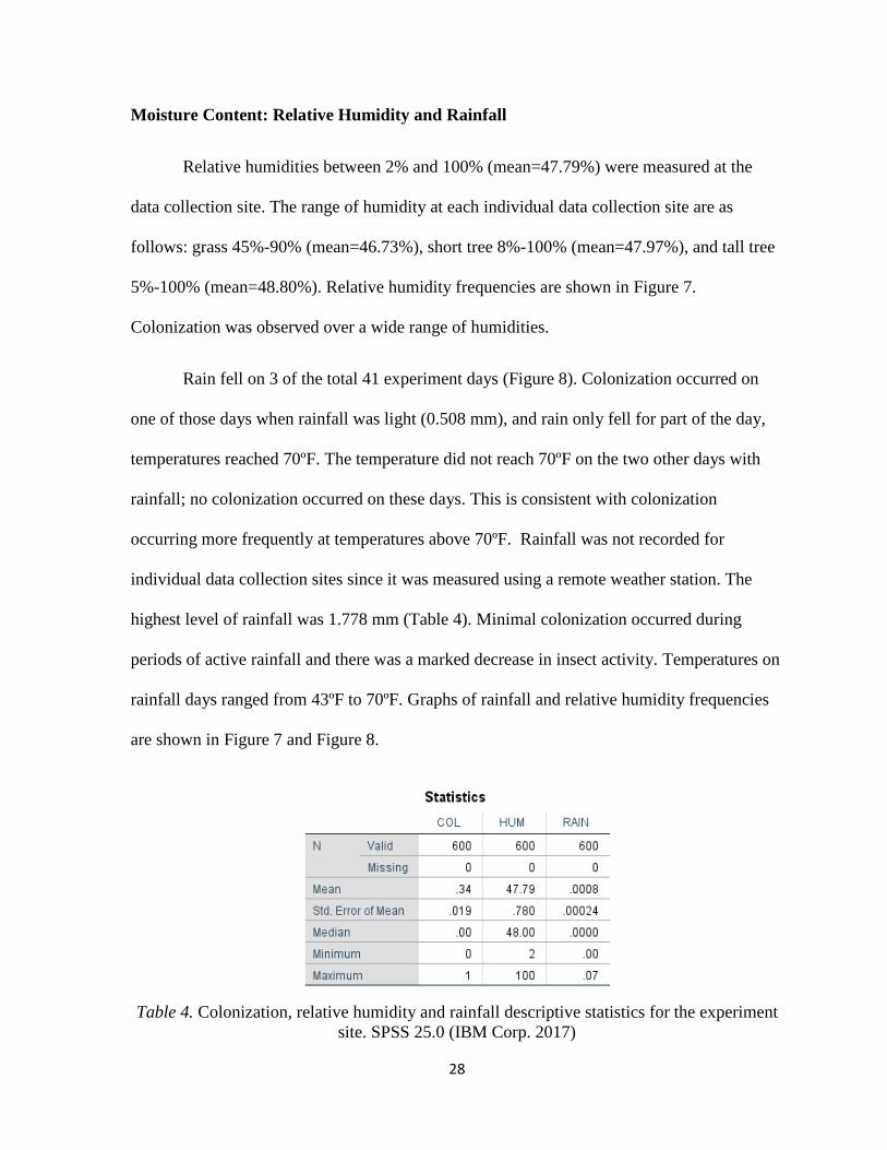
Moisture Content: Relative Humidity and Rainfall

Relative humidities between 2% and 100% (mean=47.79%) were measured at the

data collection site. The range of humidity at each individual data collection site are as

follows: grass 45%-90% (mean=46.73%), short tree 8%-100% (mean=47.97%), and tall tree

5%-100% (mean=48.80%). Relative humidity frequencies are shown in Figure 7.

Colonization was observed over a wide range of humidities.

Rain fell on 3 of the total 41 experiment days (Figure 8). Colonization occurred on

one of those days when rainfall was light (0.508 mm), and rain only fell for part of the day,

temperatures reached 70ºF. The temperature did not reach 70ºF on the two other days with

rainfall; no colonization occurred on these days. This is consistent with colonization

occurring more frequently at temperatures above 70ºF. Rainfall was not recorded for

individual data collection sites since it was measured using a remote weather station. The

highest level of rainfall was 1.778 mm (Table 4). Minimal colonization occurred during

periods of active rainfall and there was a marked decrease in insect activity. Temperatures on

rainfall days ranged from 43ºF to 70ºF. Graphs of rainfall and relative humidity frequencies

are shown in Figure 7 and Figure 8.

Table 4. Colonization, relative humidity and rainfall descriptive statistics for the experiment

site. SPSS 25.0 (IBM Corp. 2017)

29

Figure 7. Graph of relative humidity frequencies for the experiment site.

SPSS 25.0 (IBM Corp. 2017)

Figure 8. Graph of rainfall frequencies for the experiment site. SPSS 25.0 (IBM Corp. 2017)

Maximum Wind Speed

Wind speed measured (Table 5)remotely for all data collection sites ranged from

0mph to 18mph (mean=3.73mph). Wind speed relative frequencies are shown in Figure 9.

Bait was colonized during both minimal and higher recorded wind speeds. Flies most likely

could not walk to the bait due to the water moat under the bait bowl, therefore they must be

able to fly at these wind speeds since colonization still occurred.

30

Table 5. Colonization and wind speed descriptive statistics for the experiment site. SPSS 25.0

(IBM Corp. 2017)

Figure 9. Graph of wind speed frequencies for the experiment site. SPSS 25.0 (IBM Corp.

2017)

Barometric Pressure

Barometric pressure data was taken from a remote weather station. Barometric

pressure ranged from 1004.7hPa to 1024hPa (mean=1015.67hPa) (Table 6). Barometric

pressure frequencies are shown in Figure 10. Colonization was recorded over a wide range

of barometric pressure.

31

Table 6. Colonization and barometric pressure descriptive statistics for the experiment site.


Figure 10. Graph of barometric pressure frequencies for the experiment site. SPSS 25.0

(IBM Corp. 2017)

Light Intensity

Light intensity measured ranged from 100 Lux to 125,100 Lux (mean=24,611.00

Lux) (Table 8). Light intensity ranges measured (frequencies shown in Figure 11) at

individual data collection sites were as follows: grass 100 Lux to 125,100 Lux

(mean=49.242.36 Lux), short tree 100 Lux to 113,700 Lux (mean=15,698.48 Lux), and tall

tree 100 Lux to 115,700 Lux (mean=8352.27 Lux). Reference levels for light intensity are

shown in Table 7.

32

Light Intensity Lux

Overcast 1000

Full Daylight 10,000

Very Bright 100,000

Table 7. Light intensity levels for reference. (“How to Measure Light” 2016)

Table 8. Colonization and light intensity descriptive statistics for the experiment site. SPSS

25.0 (IBM Corp. 2017)

Figure 11. Graph of light intensity frequencies for the experiment site. SPSS 25.0 (IBM

Corp. 2017)

Habitat Preference

This research study was conducted in three habitat types: grass, short tree, and tall

tree. Colonization comparisons of probability based on site are shown in Table 9. Differences

in sample sizes reflect the interruption of data collection due to predation by felids. At the

grass data collection site, colonization was observed for 82 of the 203 total observations

33

(40.4%). At the short tree data collection site, colonization was observed for 69 of the 198

total observations (34.8%). At the tall tree data collection site, colonization events were

observed for 55 out of 199 total observations (27.6%). The data shows that blow flies prefer

the liver placed in the grass. This is most likely due to higher mean ambient temperatures and

light intensities at the grass site since an increase in these variables equals an increase in the

probability of colonization. The mean ambient temperature at the tall tree site was 72.86°F

and the mean light intensity was 8352.27 Lux. The mean ambient temperature at the short

tree site was 73.82°F the mean light intensity was 15,698.48 Lux. The mean ambient

temperature at the grass site was 77.44°F and the mean light intensity was 49,242.36 Lux.

While habitat type can affect climatic conditions, colonization is more likely dependent on

temperature, relative humidity, and light intensity rather than habitat type.

Table 9. The frequency of colonization for each habitat for the experiment site. SPSS 25.0

(IBM Corp. 2017)

34

Chapter 7: Statistical Analysis of Calliphorid Colonization

Binary Logistic Regression Definition and Uses

Binary logistic regression is an application of a generalized linear model used when

the dependent (response) variable is dichotomous (Quinn and Keough 2002). The predictor

variables are either continuous or categorical. Logistic regression examines the relationship

between the dependent and predictor variables. In the case of this research study, logistic

regression looks at the relationship between colonization, climatic conditions and light

intensities. The dependent variable (colonization) is a binary variable. Colonization occurred

(1) or it did not occur (0). The independent variables (ambient temperature, light intensity,

wind speed, rainfall, relative humidity, and barometric pressure) are continuous variables.

Assumptions for Logistic Regression

Data collected in this experiment meets the assumptions for analysis using logistic

regression which is: minimal missing values (data has no missing values), a sample size

greater than 50 (n=600) and, no strong collinearity between independent variables (see

section on collinearity analysis). Data collected were analyzed through backward stepwise

logistic regression using the Statistical Package for the Social Sciences or SPSS 25.0 (IBM

Corp. 2017) to model the effects of barometric pressure, ambient temperature, light intensity,

wind speed, and rainfall on the probability of bait colonization by blow flies and to create an

equation of colonization probability.

Collinearity Analysis Results

Collinearity diagnostics (Figure 12) were run in SPSS 25.0 (IBM Corp. 2017)

between the independent variables (ambient temperature, relative humidity, rainfall, wind

35

speed, barometric pressure, light intensity). Variance inflation factor (VIF) results (Table 10)

were all greater than 1.0 but less than 2.0 indicating a relatively small amount of collinearity,

but not enough to assume that any of the independent variables were acting together to

account for the variability in the dependent variable (colonization) (Schober, Boer, and

Schwarte 2018).

VIF TEMP HUMIDITY LIGHT RAIN WIND BARO

TEMP 1.387 1.856 1.963 1.788 1.951

HUMIDITY 1.214 1.778 1.753 1.706 1.624

LIGHT 1.093 1.197 1.195 1.193 1.158

RAIN 1.092 1.114 1.129 1.130 1.129

WIND 1.016 1.108 1.151 1.154 1.128

BARO 1.104 1.049 1.110 1.146 1.122

Table 10. Collinearity diagnostics results showing VIF all greater than 1.0 but less than 2.0

indicating a relatively small amount of collinearity. SPSS 25.0 (IBM Corp. 2017)

Figure 12. Graph of collinearity diagnostics results showing VIF all greater than 1.0 but less

than 2.0 indicating a relatively small amount of collinearity. SPSS 25.0 (IBM Corp. 2017)

Correlation Analysis Results

Analysis of correlation was completed using Pearson’s correlation test in SPSS 25.0

(IBM Corp. 2017) to determine if a correlation exists between the independent variables

(ambient temperature, relative humidity, rainfall, wind speed, barometric pressure, light

intensity) and assess the relationship between ambient temperature and relative humidity.

0.000

1.000

2.000

3.000

TEMP HUMIDITY LIGHT RAIN WIND BARO

Collinearity Diagnostic Stats

TEMP HUMIDITY LIGHT RAIN WIND BARO

36

Four assumptions must be met to use Pearson’s correlation test: The variables being tested

must be continuous. Variables must have a linear relationship. There must be no significant

outliers. The variables must be approximately normally distributed (Quinn and Keough

2002).

All independent variables in this study are continuous. To test their linear

relationships, I plotted the variables on scatterplots (Figures 13a-17). Temperature and

relative humidity are the only independent variables with a linear relationship. Using SPSS

25.0 (IBM Corp. 2017).

Table 11. Correlation Statistics showing a moderate negative correlation between

temperature and relative humidity, r=-596, p<0.01 with humidity explaining 35.6% of the

variability in temperature. SPSS 25.0 (IBM Corp. 2017)

There was a moderate negative correlation between temperature and humidity, r=-

596, p<0.01 with humidity explaining 35.6% of the variability in temperature. Since the

absolute value of Pearson’s correlation is less than 0.8 and collinearity tests showed no major

collinearity (Table 11), I chose to include relative humidity when running my logistic

regression statistics, since data collected show colonization throughout a range of humidities.

37

Figure 13a. Collinearity scatterplot showing no linear relationship between temperature and

light intensity. SPSS 25.0 (IBM Corp. 2017)

Figure 13b. Collinearity scatterplot showing a linear relationship between temperature and

relative humidity. SPSS 25.0 (IBM Corp. 2017)

Figure 13c. Collinearity scatterplot showing no linear relationship between temperature and

rainfall. SPSS 25.0 (IBM Corp. 2017)

38

Figure 13d. Collinearity scatterplot showing no linear relationship between temperature and

barometric pressure. SPSS 25.0 (IBM Corp. 2017)

Figure 13e. Collinearity scatterplot showing no linear relationship between temperature and

wind speed. SPSS 25.0 (IBM Corp. 2017)

Figure 14a. Collinearity scatterplot showing no linear relationship between relative

humidity and light intensity. SPSS 25.0 (IBM Corp. 2017)

39

Figure 14b. Collinearity scatterplot showing no linear relationship between relative humidity

and wind speed. SPSS 25.0 (IBM Corp. 2017)

Figure 14c. Collinearity scatterplot showing no linear relationship between relative humidity

and rainfall. SPSS 25.0 (IBM Corp. 2017)

Figure 14d. Collinearity scatterplot showing no linear relationship between relative humidity

and barometric pressure. SPSS 25.0 (IBM Corp. 2017)

40

Figure 15a. Collinearity scatterplot showing no linear relationship between light intensity

and rainfall. SPSS 25.0 (IBM Corp. 2017)

Figure 15b. Collinearity scatterplot showing no linear relationship between light intensity

and wind speed. SPSS 25.0 (IBM Corp. 2017)

Figure 15c. Collinearity scatterplot showing no linear relationship between light intensity

and barometric pressure. SPSS 25.0 (IBM Corp. 2017)

41

Figure 16a. Collinearity scatterplot showing no linear relationship between rainfall and wind

speed. SPSS 25.0 (IBM Corp. 2017)

Figure 16b. Collinearity scatterplot showing no linear relationship between rainfall and

barometric pressure. SPSS 25.0 (IBM Corp. 2017)

Figure 17: Collinearity scatterplot showing no linear relationship wind speed and barometric

pressure. SPSS 25.0 (IBM Corp. 2017)

42

Binary Logistic Regression Results

For the purposes of this study, the hypotheses being investigated are H0: Climatic

conditions and light intensities have no influence on blow fly colonization and H1: Climatic

conditions and light intensities have a significant influence on blow fly colonization. Logistic

regression was completed for each individual data collection site (tall tree, short tree, and

grass) as well as the experiment site as a whole.

Tall Tree Data Collection Site

The results of the binary logistic regression model (Figure 18) show that ambient

temperature and light intensity are significant predictor variables while barometric pressure,

relative humidity, wind speed, and rainfall are not significant predictor variables. All 199

cases were included in this model. The total percentage of correctly predicted colonization by

this model for the tall tree site was 73.9% with 97.9% predicted correctly (Figure 20) for no

colonization and 10.9% predicted correctly for colonization. The null model (Figure 19)

correctly predicted colonization 72.4% of the time.

.

Figure 18. Logistic regression case processing summary for the tall tree data collection site.


43

Figure 19. Null model (no independent variables included) shows an overall 72.4% correct

prediction of colonization for the tall tree data collection site. SPSS 25.0 (IBM Corp. 2017)

Figure 20. Model 1 (with all independent variables included) showing an overall 73.9%

correct prediction of colonization for the tall tree data collection site. SPSS 25.0 (IBM Corp.

2017)

Final probability equations for the tall tree data collection site are as follows:

Temperature: PColonization=𝑒(−0.142)+(0.005)(75°F)

1+𝑒(−0.142)+(0.005)(75°F)

Light Intensity: PColonization=𝑒(−0.142)+(3.0873𝐸−6)(24000 𝐿𝑢𝑥)

1+𝑒(−0.142)+(3.0873𝐸−6)(24000 𝐿𝑢𝑥)

44

Short Tree Data Collection Site



relative humidity, wind speed, and rainfall are not significant predictor variables. All 198

cases were included in this model. The total percentage of correctly predicted colonization by

this model (Figure 23) for the short tree site was 71.2% with 96.1% predicted correctly for no



Figure 21. Logistic regression case processing summary for the short tree data collection site.

(SPSS 25.0 (IBM Corp. 2017)

Figure 22. Null model (no independent variables included) showing an overall 65.2% correct

prediction of colonization for the short tree data collection site. SPSS 25.0 (IBM Corp. 2017)

45

Figure 23. Model 1 (all independent variables included) showing an overall 71.2% correct

prediction of colonization for the short tree data collection site. SPSS 25.0 (IBM Corp. 2017)

Final probability equations for the short tree data collection site are as follows:


1+𝑒(−1.241)+(0.017)(75°F)


1+𝑒(−1.241)+(2.829𝐸−6)(24000 𝐿𝑢𝑥)

Humidity: PColonization=𝑒(−1.241)+(0.005)(48%)

1+𝑒(−1.241)+(0.005)(48%)

Grass Data Collection Site



relative humidity, wind speed, rainfall are not significant predictor variables. All 203 cases

were included in this model. The total percentage of correctly predicted colonization by this

model (Figure 26) for the grass site was 65.0% with 76.0% predicted correctly for no



46

Figure 24. Logistic regression case processing summary for the grass data collection site.


Figure 25. Null model (no independent variables included) showing an overall 59.6% correct

prediction of colonization for the grass data collection site. SPSS 25.0 (IBM Corp. 2017)


prediction of colonization for the grass data collection site. SPSS 25.0 (IBM Corp. 2017)

47

Final probability equations for the grass data collection site are as follows:


1+𝑒(−1.416)+(0.018)(75°F)


1+𝑒(−1.416)+(0.009)(48%)

Experiment Site as a Whole

The results of the binary logistic regression model for all data collection sites

combined show that ambient temperature and light intensity are significant predictor

variables while barometric pressure, relative humidity, wind speed, and rainfall are not

significant predictor variables. All 600 cases were included in this model (Figure 27). The

total percentage of correctly predicted colonization by this model (Figure 29) for the

experiment site was 69.0% with 91.9% predicted correctly for no colonization and 25.2%

predicted correctly for colonization. The null model (Figure 28) correctly predicted

colonization 65.7% of the time.

Figure 27. Logistic regression case processing summary for the experiment site. SPSS 25.0

(IBM Corp. 2017)

48

Figure 28. Null model (no independent variables included)showing an overall 65.7% correct

prediction of colonization for the experiment site. SPSS 25.0 (IBM Corp. 2017)


prediction of colonization for the experiment site. SPSS 25.0 (IBM Corp. 2017)

Final probability equations for the data collection site are as follows:


1+𝑒(−0.894)+(0.012)(75°F)


1+𝑒(−0.894)+(1.973𝐸−6)(24000 𝐿𝑢𝑥)


1+𝑒(−0.894)+(0.005)(48%)

49

Backward Stepwise Logistic Regression Results

Colonization data were also examined using backward stepwise logistic regression.

Backward stepwise logistic regression removes any predictor variable that does not

contribute to the accuracy of the model (colonization prediction) from the regression

equation in the order in which corresponds to their importance in the equation. Data were

analyzed separately for each data collection site within the larger experiment site as well as

combined to analyze the experiment site as a whole.


Table 12. Descriptive statistics for the tall tree data collection site. SPSS 25.0 (IBM Corp.

2017)

As seen in Figure 30, wind speed, rainfall, barometric pressure, and relative humidity

were removed from the regression equation in that order which corresponded with their

importance in the equation (p=>.100). Wind speed was the least influential variable, so it was

removed in the first step, followed by rainfall, barometric pressure, and relative humidity.

According to the regression equation (Figure 31), light intensity and ambient temperature are

the factors that contribute most significantly to the colonization model for the tall tree data

collection site.

50

Figure 30. Variables entered and removed in successive steps from the logistic

regression model for the tall tree data collection site. SPSS 25.0 (IBM Corp. 2017)

Figure 31. Model summary results for the tall tree data collection site. Light intensity

and ambient temperature are significant predictor variables of colonization. SPSS 25.0 (IBM

Corp. 2017)

51


Table 13. Descriptive statistics for the short tree data collection site. SPSS 25.0 (IBM Corp.

2017).

The short tree data collection site sample size was 198 (Table 13). Wind speed,

rainfall, and barometric pressure were removed from the regression equation (Figure 32) in

that order which corresponded with their importance in the equation (p=>.100). Wind speed

was the least influential variable followed by rainfall and barometric pressure. According to

the regression equation, light intensity, ambient temperature, and relative humidity are the

factors that contribute most significantly to the colonization model (Figure 3) for the short

tree data collection site.

52


regression model for the short tree data collection site. SPSS 25.0 (IBM Corp. 2017)

Figure 33. Model summary results for the short tree data collection site. Light

intensity and ambient temperature are significant predictor variables of colonization. SPSS

25.0 (IBM Corp. 2017)


The grass date collection sample size was 203 (Table 14). Barometric pressure, wind

speed, rainfall, and light intensity were removed from the regression equation (Figure 34) in

that order which corresponded with their importance in the equation (p=>.100). Barometric

pressure was the least influential variable followed by wind speed, rainfall, and light

intensity. According to the regression equation (Figure 35), ambient temperature and relative

53

humidity are the factors that contribute most significantly to the colonization model for the

grass data collection site.

Table 14. Descriptive statistics for the grass data collection site. SPSS 25.0 (IBM Corp.

2017)


regression model for the grass data collection site. SPSS 25.0 (IBM Corp. 2017)

54

Figure 35. Model summary results for the grass data collection site. Light intensity

and ambient temperature are significant predictor variables of colonization. SPSS 25.0 (IBM

Corp. 2017)


Table 15. Descriptive statistics for logistic regression testing all variables. (SPSS 25.0 (IBM

Corp. 2017)

The sample size for the experiment site as a whole is 600 (Table 15). Results of

logistic regression of data for the experiment site show that ambient temperature, relative

humidity, and light intensity are positive predictor variables. Temperature is a more

significant predictor of colonization than is light intensity and relative humidity. George,

Archer, and Toop (2013b) found that relative humidity was a negative predictor value, but

this was not the case in my study as colonization occurred throughout a range of relative

55

humidities. Relative humidity even acc accounted for significant variance at short tree data

collection site.

Barometric pressure, wind speed, and rainfall were removed from the regression

equation (Figure 36) in that order which corresponded with their importance in the equation

(p=>.100). Barometric pressure was the least influential variable followed by wind speed and

rainfall. According to the regression equation (Figure 37), ambient temperature, light

intensity, and relative humidity are the factors that contribute most significantly to the

colonization model.


regression model for all data from the experiment site. SPSS 25.0 (IBM Corp. 2017)

56

Figure 37. Model summary results for all data from the experiment site. Light

intensity and ambient temperature are significant predictor variables of colonization. SPSS

25.0 (IBM Corp. 2017)

Predicted Probability of Colonization


An increase of 1º Fahrenheit of ambient temperature increases the probability of

colonization by 0.005. The predicted probability of colonization within 90 minutes at 75ºF,

the average observed temperature, is 0.5580 or 55.8% (Figure 38a). An increase in light

intensity by 1 Lux increases the probability of colonization by 3.0870E-6. The predicted

probability of colonization within 90 minutes at 24,000 Lux, the average observed light

intensity, is 0.4830 or 48.3% (Figure 38b). Colonization probabilities are calculated using an

Excel spreadsheet (Table 16.)

57

TEMPERATURE Average

Variable Coefficient 60°F 70°F 75°F 85°F 90°F

Constant -0.142 1 1 1 1 1

Temperature 0.005 60 70 75 85 90

y*=ln(p/(1-p)) 0.16 0.21 0.23 0.28 0.31

p=exp(y*)/(exp(y*)+1) 0.5394 0.5518 0.5580 0.5703 0.5764

Probability 54.0% 55.2% 55.8% 57.0% 58.0%

Change 0.01240 0.00617 0.01229 0.00612

LIGHT INTENSITY overcast full light Average very bright

Variable Coefficient

1000

Lux

10000

Lux

24000

Lux

50000

Lux

100000

Lux

Constant -0.142 1 1 1 1 1

Light Intensity 0.0000030870 1000 10000 24000 50000 100000

y*=ln(p/(1-p)) -0.1389 -0.1111 -0.0679 0.0124 0.1667

p=exp(y*)/(exp(y*)+1) 0.4653 0.4722 0.4830 0.5031 0.5416

Probability 46.5% 47.2% 48.3% 50.3% 54.2%

Change 0.00692 0.01078 0.02006 0.03849

Table 16. The predicted probability of colonization within 90 minutes at various ambient

temperatures and light intensities for the tall tree data collection site. Values for constant and

coefficients are unstandardized coefficients generated during backward stepwise logistic

regression.

Figure 38a. The probability of colonization at selected ambient temperatures for the tall tree

data collection site.

0.5

0.55

0.6

60°F 70°F 75°F 85°F 90°F

Probability of Colonization at

Selected …

58

Figure 38b. The probability of colonization at selected light intensities for the tall tree data

collection site.





intensity by 1 Lux increases the probability of colonization by 2.8290E-6 (Figure 39b). The

predicted probability of colonization within 90 minutes at 24,000 Lux, the average observed

light intensity, is 0.2363 or 24.0%. An increase in relative humidity by 1% increases the

probability of colonization by 0.005. The predicted probability of colonization within 90

minutes at 48% relative humidity, the average observed relative humidity, is 0.2687 or 27.0%

(Figure 39c). Colonization probabilities are calculated using an Excel spreadsheet (Table 17.)

0.4

0.6

1000 10000 24000 50000 100000

LIGHT INTENSITY (LUX)

Probability of Colonization at Selected Light …

59

TEMPERATURE Average


Constant -1.241 1 1 1 1 1

Temperature 0.017 60 70 75 85 90

y*=ln(p/(1-p)) -0.22 -0.05 0.03 0.20 0.29

p=exp(y*)/(exp(y*)+1) 0.4450 0.4873 0.5085 0.5508 0.5718

Probability 44.5% 48.7% 51.0% 55.1% 57.2%

Change 0.04228 0.02125 0.04232 0.02093

LIGHT INTENSITY overcast full light Average

very

bright


1000

Lux

10000

Lux

24000

Lux

50000

Lux

100000

Lux

Constant -1.241 1 1 1 1 1

Light Intensity 0.0000028290 1000 10000 24000 50000 100000

y*=ln(p/(1-p)) -1.2382 -1.2127 -1.1731 -1.0996 -0.9581

p=exp(y*)/(exp(y*)+1) 0.2248 0.2292 0.2363 0.2498 0.2773

Probability 22.5% 23.0% 24.0% 25.0% 28.0%

Change 0.00447 0.00707 0.01353 0.02743

HUMIDITY Average

Variable Coefficient 25.00 35.00 48.00 65.00 85.00

Constant -1.241 1 1 1 1 1

Humidity 0.005 25 35 48 65 85

y*=ln(p/(1-p)) -1.1160 -1.0660 -1.0010 -0.9160 -0.8160

p=exp(y*)/(exp(y*)+1) 0.2468 0.2562 0.2687 0.2858 0.3066

Probability 25.0% 26.0% 27.0% 29.0% 31.0%

Change 0.00941 0.01258 0.01703 0.02084


temperatures and light intensities for the short tree data collection site. Values for constant

and coefficients are unstandardized coefficients generated during backward stepwise logistic

regression.

60

Figure 39a. The probability of colonization at selected ambient temperatures for the short

tree data collection site.

Figure 39b. The probability of colonization at selected light intensities for the short tree data

collection site.

Figure 39c. The probability of colonization at selected relative humidities for the short tree

data collection site.

0

0.5

1

60°F 70°F 75°F 85°F 90°F


Selected …

0

0.5

1000 10000 24000 50000 100000



0

0.5

0.25 0.35 0.48 0.65 0.85

HUMIDITY


Selected Humidities

61




the average observed temperature, is 0.4835 or 49.3% (Figure 40a). An increase in relative

humidity by 1% increases the probability of colonization by 0.009. The predicted probability

of colonization within 90 minutes at 48% relative humidity, the average observed relative

humidity, is 0.2721 or 27.2% (Figure 40b). Colonization probabilities are calculated using an

Excel spreadsheet (Table 18.)

TEMPERATURE Average


Constant -1.416 1 1 1 1 1

Temperature 0.018 60 70 75 85 90

y*=ln(p/(1-p)) -0.34 -0.16 -0.07 0.11 0.20

p=exp(y*)/(exp(y*)+1) 0.4168 0.4611 0.4835 0.5285 0.5508

Probability 41.7% 46.1% 48.4% 53.0% 55.1%

Change 0.04430 0.02243 0.04496 0.02235

HUMIDITY Average


Constant -1.416 1 1 1 1 1

Humidity 0.009 25 35 48 65 85

y*=ln(p/(1-p))

-

1.1910 -1.1010 -0.9840 -0.8310 -0.6510

p=exp(y*)/(exp(y*)+1) 0.2331 0.2496 0.2721 0.3034 0.3428

Probability 23.3% 25.0% 27.2% 30.3% 34.3%

Change 0.01647 0.02255 0.03133 0.03933


temperatures and light intensities for the grass data collection site. Values for constant and

coefficients are unstandardized coefficients generated during backward stepwise logistic

regression.

62

Figure 40a. The probability of colonization at selected ambient temperatures grass data

collection site.

Figure 40b. The probability of colonization at selected relative humidities at the grass data

collection site.





intensity by 1 Lux increases the probability of colonization by 1.9730E-6. The predicted

probability of colonization within 90 minutes at 24,000 Lux, the average observed light

intensity, is 0.3001 or 30.0% (Figure 41b). An increase in relative humidity by 1% increases

0

0.5

1

60°F 70°F 75°F 85°F 90°F


Selected …

00.20.4

0.25 0.35 0.48 0.65 0.85HUMIDITY


Selected Humidities

63

the probability of colonization by 0.005. The predicted probability of colonization within 90

minutes at 48% relative humidity, the average observed relative humidity, is 0.3421 or 34.3%

(Figure 41c). Colonization probabilities are calculated using an Excel spreadsheet (Table 19.)

TEMPERATURE Average


Constant -0.894 1 1 1 1 1

Temperature 0.012 60 70 75 85 90

y*=ln(p/(1-p)) -0.17 -0.05 0.01 0.13 0.19

p=exp(y*)/(exp(y*)+1) 0.4566 0.4865 0.5015 0.5315 0.5464

Probability 45.7% 48.7% 50.2% 53.2% 54.6%

Change 0.02989 0.01500 0.02996 0.01491

LIGHT INTENSITY Overcast

Full

light Average

Very

bright


1000

Lux

10000

Lux

24000

Lux

50000

Lux

100000

Lux

Constant -0.894 1 1 1 1 1

Light Intensity 0.0000019730 1000 10000 24000 50000 100000

y*=ln(p/(1-p)) -0.8920 -0.8743 -0.8466 -0.7954 -0.6967

p=exp(y*)/(exp(y*)+1) 0.2907 0.2944 0.3001 0.3110 0.3325

Probability 29.1% 29.4% 30.0% 31.1% 33.3%

Change 0.00367 0.00577 0.01088 0.02152 HUMIDITY Average


Constant -0.894 1 1 1 1 1

Humidity 0.005 25 35 48 65 85

y*=ln(p/(1-p)) -0.7690 -0.7190 -0.6540 -0.5690 -0.4690

p=exp(y*)/(exp(y*)+1) 0.3167 0.3276 0.3421 0.3615 0.3849

Probability 32.7% 32.8% 34.2% 36.2% 38.5%

Change 0.01092 0.01448 0.01938 0.02339


temperatures, light intensities, and relative humidities for the experiment site. Values for

constant and coefficients are unstandardized coefficients generated during backward stepwise

logistic regression.

64

Figure 41a. The probability of colonization at selected ambient temperatures for the

experiment site.

Figure 41b. The probability of colonization at selected light intensities for the experiment

site.

Figure 41c. The probability of colonization at selected relative humidities for the experiment

site.

40.0%

50.0%

60.0%

60°F 70°F 75°F 85°F 90°F


Selected …

20.0%30.0%40.0%

1000 10000 24000 50000 100000



20.0%30.0%40.0%

25% 35% 48% 65% 85%

HUMIDITY


Selected Humidities

65

Analysis of Probability

The tall tree data collection site had a slightly higher probability of colonization at the

average temperature (75 ºF) at 55.8% compared to the short tree site at 51.0% and 48.49%

for the grass data collection site. At the average light intensity (24,000 Lux), the tall tree data

collection site also had a higher probability of colonization at 48.3% compared to 24.0% at

the short tree data collection site. The grass site was not included in this analysis because

light intensity was removed as a significant predictor variable in the logistic regression

equation. Comparison of the probability of colonization at the average of 48% relative

humidity shows that the short tree data collection site had the highest probability of

colonization at 27.0% while it was 27.2% at the grass data collection site. The tall tree site

was not included in this comparison because relative humidity was not included as a

significant predictor variable in the logistic regression equation.

Accumulated Degree Days (ADD)

Utilizing the method for calculating ADD with a minimum threshold temperature of

70ºF (Mann, Bass, and Meadows 1990), colonization should have occurred on 33 out of the

41 days or 80% of the days. My study had 30 days of the 41 total where colonization

occurred or a 73% colonization rate. The ADD method was accurate for 28 of the 41 days or

68%. It incorrectly predicted colonization 13 out of the 41 days or 32% of the time.

Activity Patterns

A total of 600 observations were made at the experiment site with an overall 34%

colonization rate. A total of 199 observations were made at the tall tree data collection site

with a 28% colonization rate. A total of 198 observations were made at the short tree data

66

collection site with a 35% colonization rate. A total of 203 observations were made at the

grass data collection site with a 40% colonization rate. These observations were made under

a range of climatic conditions, over the course of several months in successive years (Figure

42), and thus allows the construction of a set of parameters in which colonization did or did

not occur.

Figure 42. Colonization events by month showing a spike in colonization in summer months.

Monthly data is pooled between years.

Similar Applications of Logistic Regression

In France, Cervantes et al. (2018) used linear regression to model the effect of low

temperatures on the development and egg-laying habits of the blow fly Lucilia sericata and

its implications on the estimation of the postmortem interval. Their attempts to create a

global linear model showed an overestimation of the effects of some temperatures on

development and egg laying.

Zurawski at al. (2009) used both forward and backward stepwise logistic regression

to study nocturnal oviposition behavior of blowflies in Michigan. Predictor variables were

removed from the logistic regression model based on the significance of influence on egg

laying at night. Their final regression model included wind speed, ambient temperature, and

0

50

100

Colonization Events by Month

67

relative humidity, but not light intensity. They concluded that ambient temperature and

relative humidity, as well as ambient temperature and light intensity, were positively

correlated and that the significance of light intensity depends on ambient temperature and

relative humidity.

Barnes et al. (2015) used backward stepwise logistic regression to model the behavior

of blow flies at night in England. Nocturnal oviposition did not occur during their data

collection period. Ambient temperature was found to be the only significant predictor

variable in their study and contrary to Zurawski et al., Barnes et al. concluded that

temperature and relative humidity were negatively correlated.

George, Archer, and Toop (2013) modeled the influence of abiotic factors on

colonization by blow flies using backward stepwise logistic regression in Victoria, Australia.

Barometric pressure, light intensity, rainfall, and wind speed were removed from their

regression model in with barometric pressure having the lease effect on colonization.

Ambient temperature and relative humidity were found to be significant predictor variables.

George, Archer, and Toop (2013b) also determined that temperature and relative humidity

were negatively correlated.

68

Chapter 8: Species Observed

Bluebottle fly

Bluebottle flies (Calliphora vicina) are found throughout the United States and

Canada. Its size ranges from 1/4" to 1/2“ long. Bluebottle flies are dark blue to black, very

hairy and have a metallic glint (Byrd and Castner 2000). This fly is often found on human

remains in urban areas and buzzes loudly. This species was commonly observed during my

41 days of data collection (Figure 43).

Figure 43. Bluebottle flies (Calliphora vicina) on the edge of the bait bowl.

(Photo by author)

Shiny Bluebottle Fly

Shiny bluebottle flies (Cynomyopsis caderverina) are very common and can be found

throughout the United States, particularly in wooded and rural areas. They range in size from

1/3” to 1/2" long. Shiny bluebottle flies are metallic dark blue to blue-black with a shiny blue

abdomen (Byrd and Castner 2000). This species was commonly observed during my 41 days

of data collection (Figure 44).

69

Figure 44. Shiny Bluebottle Fly (Cynomyopsis caderverina) on colonization medium.

(Photo by author)

Greenbottle Fly

Greenbottle flies (Lucilia sericata) are common throughout the United States,

particularly in rural and wooded areas. They are 1/4" to 3/8” in length. They are metallic

green to blue-green. They are often found at fresh remains (Byrd and Castner 2000). This

species was the most commonly observed species during my 41 days of data collection

(Figure 45).

Figure 45. Greenbottle Fly (Lucilia sericata) on colonization medium.

(Photo by author)

70

Cheese Skipper Fly

Cheese skipper flies (Piophila casei) are distributed throughout the United States and

Canada. They are 1/8” to 1/4” length. Their body is black or to metallic blue (Byrd and

Castner 2000). This species shows up late in succession and does not necessarily indicate

colonization. A single cheese skipper was observed during the review of photos taken during

data collection (Figure 46).

Figure 46. Cheese skipper (Piophila casei) on colonization medium.

(Photo by author)

Red-tailed Flesh Fly

Red-tailed flesh flies (Sarcophaga haemorrhoidalis) are found worldwide and are

associated with human remains in the United States and Canada. Adult flesh flies are up to

3/4” in length. They have gray and black longitudinal stripes on the thorax and a

checkerboard pattern on the abdomen. They lack the metallic coloration of blow flies (Byrd

and Castner 2010). Some species have bright red compound eyes. Adult females lay live

first-instar larva in excrement and on dead animals (Byrd and Castner 2010). This species

was seen more often in photos taken during data collection than actually observed on the bait

71

during my 41 days of data collection. Larvae, possibly from the red-tailed flesh fly, were

observed twice during data collection (Figure 47).

Figure 47. Red-tailed flesh fly (Sarcophaga haemorrhoidalis) on colonization medium.

(Photo by author)

72

Chapter 9: Unanticipated Confounding Factors

Scavenging by Felids

Scavenging of the bait liver by a housecat (Family: Felidae) occurred early on in the

data collection process. Felid scavenging was observed on two days during the 41 days of my

research study, twice in one day which interrupted data collection. This issue was resolved by

adding a second plastic basket over the bait, turning the baskets in opposite directions so that

the holes overlapped on the sides creating smaller openings and then placing heavier weights

on top of the baskets.

Predation of Eggs and Flies by Insects

Predators of fly eggs, larvae and of adult flies include silphids (burying beetles),

histerids (hister beetles), and formicids (ants) (Greenberg 1991). Beetles, hornets, and

yellowjackets were observed in or around the bait bowl. Ants were observed in the water

moat under the bait bowl.

A single multicolored Asian lady beetle larva (Harmonia axyridis) (Figure 48) was

observed on an egg mass, possibly eating the eggs. Asian lady beetles were introduced into

the United States to control aphids (Jacobs 2013). Asian lady beetle larvae are long, flat and

covered in tubercles or spines (Jacobs 2013).

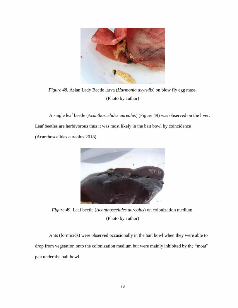
73

Figure 48. Asian Lady Beetle larva (Harmonia axyridis) on blow fly egg mass.

(Photo by author)

A single leaf beetle (Acanthoscelides aureolus) (Figure 49) was observed on the liver.

Leaf beetles are herbivorous thus it was most likely in the bait bowl by coincidence

(Acanthoscelides aureolus 2018).

Figure 49. Leaf beetle (Acanthoscelides aureolus) on colonization medium.

(Photo by author)

Ants (formicids) were observed occasionally in the bait bowl when they were able to

drop from vegetation onto the colonization medium but were mainly inhibited by the “moat”

pan under the bait bowl.

74

Yellowjackets (Vespula maculifrons) were observed in great numbers around the bait

(Figure 50), but no predation of eggs or adult flies was observed. Yellowjackets nest in the

ground and are common in many states. They are approximately 1/2” to 3/4" and are black

with yellow stripes. They can be quite aggressive when defending their nest. Data collection

sites may have been located near in-ground nests (Jacobs 2015b).

Figure 50. Yellowjackets (Vespula maculifrons) eating colonization medium.

(Photo by author)

However, predation by bald-faced hornets (Dolichovespula maculata) was observed.

There are 7 or 8 species of bald-faced hornets in North America. It is not a “true hornet,” but

is a yellowjacket. Bald-faced hornets are found in most of the contiguous United States. The

hornets are black with a white face. They range in size from 1/2’ to 3/4”. Nests are made in

the brush and shrubs. Bald-faced hornets eat live prey including flies, yellowjackets and

other insects (Jacobs 2015a).

Bald-faced hornets (Figure 51) were observed catching adult flies and yellowjackets

in mid-air and on the liver itself. Fly wings and legs were observed in the bait bowl (Figure

52).

75

Figure 51. Bald-faced hornet (Dolichovespula maculata) on colonization medium.

(Photo by author)

Figure 52. Blow fly wing and leg in bait bowl are evidence of predation by bald-faced

hornets. (Photo by author)

Blow fly activity and egg-laying continued to occur in the presence of bald-faced

hornets but was often confined to the protected areas under the bait or where bait protruded

through the drilled holes in the bottom of the bait bowl. In addition, egg masses were

relatively small or single eggs were laid instead of large batches. Data collection was difficult

at times due to the number of yellowjackets and hornets on and around the bait.

Predation of Flies by Arachnids

A crab spider (Misumena vatia) was observed in the bait bowl eating a blow fly

(Figure 53). Crab spiders are found in North America and Europe. The crab spider has a

76

short, wide and flat body with larger front legs compared to the back. They are light colored

with white, yellow or red markings. They range in size from 1/4" to 1/3” for females and 1/8”

for males (Mahmoud 2002). They do not spin webs or wrap their prey in silk. Crab spiders

hold their prey and drink their body fluids. They use venom to immobilize their prey and

often eat larger insects like bees, butterflies, and grasshoppers. Their main defense is

camouflage. This species was found in the bait bowl near a horse chestnut tree with white

blooms.

Figure 53. Crab spider (Misumena vatia) eating a blow fly.

(Photo by author)

Wildfire Smoke and Fly Activity

The impacts of fire (planned burns, wildfire and agricultural) on insects is widely

studied (New 2014; Swengel 2001), but there is little in the literature about the impact of

smoke on blow fly oviposition. The direct consequences of fire on insects, in general, is two-

fold: the loss of organisms and the loss of resources. The impact of fire may drive

populations to extinction through the elimination of individuals, eliminate entire fire

susceptible groups, reduce resources so that competition becomes important, and reduce

resource variety which may lead to the extinction of feeding specialists and increasing the

competition for those resources (New 2014).

77

Wildfires contribute to air pollution by adding particulate matter to the air. Particulate

matter or particulate pollution is the mix of solid particles and liquid droplets in the air. The

Pacific Northwest (Washington and Oregon) had a total of 67 wildfires in 2016 and 118

wildfires in 2017 (Northwest Annual Fire Report 2016; 2017). Air quality was impacted by

these wildfires. The United States Environmental Protection Agency (EPA) measures and

reports particulate matter as a public health service. This data is reported as AQI or Air

quality index (Table 20) on a scale of 0 to 500.

AQI LEVEL

0-50 Good

51-100 Moderate

101-150 Unhealthy for sensitive groups

151-200 Unhealthy

201-500 Hazardous

Table 20. Air quality index levels for reference. (“Spokane Regional Clean Air Agency” n.d.)

The Spokane Regional Clean Air Agency monitors air quality thought out Spokane

County via 6 monitoring station and reports it to the Environmental Protection Agency

(“Spokane Regional Clean Air Agency” n.d.).

According to the Spokane Regional Clean Air Agency, there were 16 days in 2017

and 0 days in 2016 when smoke from wildfires exceeded health-based air quality standards.

Wildfire smoke was observed at the data collection site 1 day in 2016 and 15 days in 2017.

On data collection days with moderate AQI, colonization occurred 8 out of 12 days. When

the AQI moved into the unhealthy for sensitive people range, colonization occurred all three

days. No colonization occurred on the only very unhealthy AQI day although temperatures

reached at least 70ºF.

78

It is unclear whether wildfire smoke had any effect on the oviposition behavior of the

blow flies in my study. There is a slight negative correlation (Table 22) between colonization

and AQI (-0.102 Pearson’s Correlation test). It is possible that the smoke and the chemicals

that comprise it inhibit the blow fly’s ability to sense VOCs. Although flies were still

observed on the smoky days (Table 21), without a count of how many flies attended the bait

each day, I have no way of knowing if there were fewer flies on the smoky days. The effect

of smoke on oviposition in blow flies is an area where more study is needed.

Table 21. Descriptive statistics AQI, ADD, and ambient temperatures vs colonization. SPSS

25.0 (IBM Corp. 2017)

Table 22. Correlation results between colonization, observation of flies, ADD, and AQI.


79

Chapter 10: Discussion and Conclusions

Ambient Temperature, Light Intensity, Relative Humidity, and Colonization

This is the first study in Eastern Washington to attempt to predict the likelihood of

bait colonization by blow flies using abiotic variables. Using logistic regression, an attempt

was made to identify which environmental factors significantly contribute to the prediction of

bait colonization within the first 60-90 minutes of bait placement. The most significant

positive predictor variable was ambient temperature. Increasing the ambient temperature

increases the probability of bait colonization. Light intensity and relative humidity also

contribute to the probability of colonization.

Other Factors Influencing Colonization

Overall colonization rates of 34% suggest that there are other factors besides ambient

temperature, light intensity, and relative humidity that influence the colonization rates of

blow flies. Although logistic regression shows that temperature is one of the most influential

predictor variables for colonization, given the relatively high prediction rate of colonization

for temperatures over 75°F (greater than 50%), it is possible that this model overestimates the

effect of ambient temperature since it does not account for these unknown variables. All

other variables aside, if a minimum threshold temperature is not met, colonization will not

occur.

Optimal Temperature Ranges for Blow Fly Colonization

While the optimal ambient temperature for egg laying and hatching is about 70ºF

(Mann, Bass, and Meadows 1990) egg laying has been observed at ambient temperatures

between 53.6 ºF and 86 ºF (Erzinclioglu 1996). Of the 206 colonization events that took

80

place, in my research study, 170 of those events occurred when temperatures were above

70°F and 36 occurred when temperatures were below 70°F and as low as 55°F (Table 23).

Analysis of temperature and colonization occurrence in this study show that the

upper-temperature range may be higher than 86ºF for the geographic region of Eastern

Washington. Temperatures over 86ºF were observed 48 times during data collection, with

colonization occurring 26 of the 48 times (54.2%) at temperatures as high as 104ºF. The

temperature range for colonization for this region of Eastern Washington would then be 55ºF

to 104ºF.

Temperatures higher than 104ºF did not occur during the experiment period and

therefore further studies may increase this upper range. Colonization was not recorded at

temperatures below 55ºF although data was collected in temperatures as low as 36ºF. The

difference in the temperature range for colonization may be due to regional behavioral

differences in species or due to species present. This is further evidence that ranges for each

geographic region must be established.

Temp

°F

Col

Events

Temp

°F

Col

Events

55 2 66 1

56 0 67 0

57 2 68 6

58 0 69 0

59 3 88 5

60 0 90 6

61 1 91 4

62 0 93 3

63 1 97 2

64 6 99 2

65 0 100 1

66 1 104 3

Table 23. The number of colonization events occurring at temperatures below 70°F and

above 86°F.

81

Conclusions

The goal of this study was to determine which abiotic environmental conditions

contribute to the probability of colonization for blow flies in Eastern Washington. Logistic

regression shows that ambient temperature, relative humidity, and light intensity contribute

to the probability of colonization. Ambient temperature contributes at a more significant

level than does relative humidity or light intensity since the predicted probability of

colonization within 90 minutes at 75ºF, the average observed temperature, is 0.5015 (50.2%)

while the predicted probability of colonization within 90 minutes at 24,000 Lux, the average

observed light intensity, is 0.3001 (30.0%) and the predicted probability of colonization

within 90 minutes at 48% relative humidity, the average observed light intensity, is 0.3421

(34.2%).

There are most likely other variables besides abiotic environmental ones that

influence the probability of colonization, perhaps some that cannot be accounted for by

statistical measurement. Given its importance in the developmental phases of the blow fly

life cycle, temperature is a significant predictor variable. Without adequate temperature,

colonization does not occur at all. Minimum and maximum points for environmental

conditions, particularly for temperature, should form the basis, or at least the beginning point,

of predicting colonization for use in estimating the postmortem interval in forensic

investigations rather than the logistic regressions used in this study. Using the minimum and

maximum points for environmental conditions could be used in any geographic region once

these thresholds were established locally and for the species present allowing for greater

accuracy in the estimation of postmortem interval.

82

Limitations and Future Studies

Maggots were not collected and grown out to identify species due to space

constraints, therefore, identification was limited to observation and review of photos taken

during data collection. This means that I was unable to distinguish eggs to species. A study

looking at which blow fly species are present in the area where this study was done as well as

a timeline of species seasonality would have been helpful.

While mammalian liver is often used in colonization studies, it might not attract blow

flies in the same way as human remains. Most oviposition studies using bait other than

human remains experience this limitation (Pritam and Jayaprakash 2009). Human remains

could possibly yield more accurate results allowing a more precise estimation of the

postmortem interval.

As a case study from a specific geographic region, this research adds to the current

knowledge of insect succession, life cycles and the effects of variables on those processes

and on decomposition as well. Clarifying the initial insect contact period is important in

estimating time since death in forensic cases. Without adequate information concerning the

period of insect activity (PIA), the understanding of the entire decomposition process is

limited. Research which expands the literature of forensic entomology and contributes to the

knowledge of legal investigations and proceedings is vital to the understanding of the initial

insect colonization of human remains to accurate estimate the postmortem interval and

establish the time of death. Insect evidence is generally accepted in legal proceedings.

Therefore, law enforcement and legal professionals in both criminal and civil investigations

seek expert opinion of forensic entomologists.

83

Gaps in the postmortem interval allow suspects in homicide cases to be included or

excluded based on evidence and alibis. The exclusion of a suspect could allow a suspect to

avoid prosecution and punishment for their crime while the inclusion of an innocent person

as a suspect could contribute to the conviction and punishment of an innocent person,

impeding the legal process. More research studies, specific to geographic regions and to blow

fly species and habitat are needed to construct a database for use in the estimation of the

postmortem interval in forensic death investigations.

84

Works Cited

Aak, A., G. Knudsen, and A. Soleng. 2010. “Wind Tunnel Behavioural Response and Field

Trapping of the Blowfly Calliphora Vicina.” Medical and Veterinary Entomology 24 (3):

250–57. https://doi.org/10.1111/j.1365-2915.2010.00872.x.

“Acanthoscelides Aureolus.” 2018. Bug Guide: Iowa State University Department of Entomology.

2018. https://bugguide.net/node/view/15567.

Amendt, J., C. Campobasso, E. Gaudry, C. Reiter, H. LeBlanc, and M. Hall. 2007. “Best Practice

in Forensic Entomology: Standards and Guidelines.” International Journal of Legal

Medicine 121 (2): 90–104. https://doi.org/10.1007/s00414-006-0086-x.

Amendt, J., C. Richards, C. Campobasso, R. Zehner, and M. Hall. 2011. “Forensic Entomology:

Applications and Limitations.” Forensic Science Medicine and Pathology 7 (4): 379–92.

https://doi.org/10.1007/s12024-010-9209-2.

Amendt, J., R. Zehner, and F. Reckel. 2008. “The Nocturnal Oviposition Behaviour of Blowflies

(Diptera: Calliphoridae) in Central Europe and Its Forensic Implications.” Forensic Science

International 175 (1): 61–64. https://doi.org/doi.org/10.1016/j.forsciint.2007.05.010.

Ames, C., and B. Turner. 2003. “Low Temperature Episodes in Development of Blowflies:

Implications for Postmortem Interval Estimation.” Medical and Veterinary Entomology 17

(2): 178–86. https://doi.org/10.1046/j.1365-2915.2003.00421.x.

Anderson, G. 2000. “Minimum and Maximum Development Rates of Some Forensically

Important Calliphoridae (Diptera).” Journal of Forensic Sciences 45 (4): 14778J.

https://doi.org/10.1520/JFS14778J.

———. 2010. “Factors That Influence Insect Succession on Carrion.” In Forensic Entomology:

The Utility of Arthropods in Legal Investigations, edited by J. Byrd and J. Castner, Second,

201. New York: CRC Press.

https://doi.org/10.1111/j.1365-2915.2010.00872.x

https://bugguide.net/node/view/15567

https://doi.org/10.1007/s00414-006-0086-x

https://doi.org/10.1007/s12024-010-9209-2

https://doi.org/doi.org/10.1016/j.forsciint.2007.05.010

https://doi.org/10.1046/j.1365-2915.2003.00421.x

https://doi.org/10.1520/JFS14778J

85

———. 2011. “Comparison of Decomposition Rates and Faunal Colonization of Carrion in

Indoor and Outdoor Environments.” Journal of Forensic Sciences 56 (1): 136–42.

https://doi.org/10.1111/j.1556-4029.2010.01539.x.

Anderson, G., and S. VanLaerhoven. 1996. “Initial Studies on Insect Succession on Carrion in

Southwestern British Columbia.” Journal of Forensic Science 41 (4): 617–25.


Anderson, G., and J. Warren. 2011. “Establishing Lower Developmental Thresholds for a

Common Blowfly: For Use in Estimating Elapsed Time since Death Using Entomological

Methods.” Government DRDC CSS CR 2011-23. Canada: Defense Research and

Development Canada. http://www.dtic.mil/dtic/tr/fulltext/u2/a553113.pdf.

Archer, M. 2003. “Annual Variation in Arrival and Departure Times of Carrion Insects at

Carcasses: Implications for Succession Studies in Forensic Entomology.” Australian Journal

of Zoology 51 (6): 569–76. https://doi.org/10.1071/ZO03053.

———. 2004. “Rainfall and Temperature Effects on the Decomposition Rate of Exposed

Neonatal Remains.” Science & Justice 44 (1): 35–41. https://doi.org/10.1016/S1355-

0306(04)71683-4.

———. 2014. “Comparative Analysis of Insect Succession Data from Victoria (Australia) Using

Summary Statistics versus Preceding Mean Ambient Temperature Models.” Journal of

Forensic Sciences 59 (2): 404–12. https://doi.org/10.1111/1556-4029.12345.

Archer, M., and M. Elgar. 2003. “Yearly Activity Patterns in Southern Victoria (Australia) of

Seasonally Active Carrion Insects.” Forensic Science International 132 (3): 173–76.

https://doi.org/10.1016/S0379-0738(03)00034-3.

https://doi.org/10.1111/j.1556-4029.2010.01539.x


http://www.dtic.mil/dtic/tr/fulltext/u2/a553113.pdf

https://doi.org/10.1071/ZO03053

https://doi.org/10.1016/S1355-0306(04)71683-4

https://doi.org/10.1016/S1355-0306(04)71683-4

https://doi.org/10.1111/1556-4029.12345

https://doi.org/10.1016/S0379-0738(03)00034-3

86

Avila, F., and M. Goff. 1998. “Arthropod Succession Patterns onto Burnt Carrion in Two

Contrasting Habitats in the Hawaiian Islands.” Journal of Forensic Sciences 43 (3): 581–86.


Azevedo, R., and R. Kruger. 2013. “The Influence of Temperature and Humidity on Abundance

and Richness of Calliphoridae (Diptera).” Iheringia Série Zoologia 103 (2): 145–52.

https://doi.org/10.1590/S0073-47212013000200010.

Baldridge, R., S. Wallace, and R. Kirkpatrick. 2006. “Investigation of Nocturnal Oviposition by

Necrophilous Flies in Central Texas.” Journal of Forensic Sciences 51 (1): 125–26.

https://doi.org/10.1111/j.1556-4029.2005.00022.x.

Baqué, M., and J. Amendt. 2012. “Strengthen Forensic Entomology in Court: The Need for Data

Exploration and the Validation of a Generalised Additive Mixed Model.” International

Journal of Legal Medicine 127 (1): 213–23. https://doi.org/10.1007/s00414-012-0675-9.

Barnes, K., K. Grace, and M. Bulling. 2015. “Nocturnal Oviposition Behavior of Forensically

Important Diptera in Central England.” Journal of Forensic Sciences 60 (6): 1601–4.

https://doi.org/10.1111/1556-4029.1284.

Beck, S. 1983. “Insect Thermoperiodism.” Annual Review of Entomology 28 (January): 91–108.

https://doi.org/10.1146/annurev.en.28.010183.000515.

Benecke, M. 2001. “A Brief History of Forensic Entomology.” Forensic Science International

120 (1–2): 2–14. https://doi.org/10.1016/S0379-0738(01)00409-1.

Berg, M., and M. Benbow. 2013. “Environmental Factors Associated with Phormia Regina

(Diptera: Calliphoridae) Oviposition.” Journal of Medical Entomology 50 (2): 451–57.

https://doi.org/10.1603/ME12188.


https://doi.org/10.1590/S0073-47212013000200010

https://doi.org/10.1111/j.1556-4029.2005.00022.x

https://doi.org/10.1007/s00414-012-0675-9

https://doi.org/10.1111/1556-4029.1284

https://doi.org/10.1146/annurev.en.28.010183.000515

https://doi.org/10.1016/S0379-0738(01)00409-1

https://doi.org/10.1603/ME12188

87

Bertomeu Sanchez, J.R. 2004. “Orfila i Rotger (1787-1853): Science, Medicine, and Crime in the

Nineteenth Century.” Contributions to Science 2 (4): 565–78.

Brundage, A., M. Benbow, and J. Tomberlin. 2014. “Priority Effects on the Life-History Traits of

Two Carrion Blow Fly (Diptera, Calliphoridae) Species.” Ecological Entomology 39 (5):

539–47. https://doi.org/10.1111/een.12128.

Bunchu, N., C. Thaipakdee, A. Vitta, S. Sanit, K. Sukontason, and K.I. Sukontason. 2012.

“Morphology and Developmental Rate of the Blow Fly, Hemipyrellia Ligurriens (Diptera:

Calliphoridae): Forensic Entomology Applications.” Journal of Parasitology Research 2012:

1–10. https://doi.org/10.1155/2012/371243.

Byers, S. 2017. Introduction to Forensic Anthropology. Fifth. Oxon, New York: Routledge.

Byrd, J., and J. Castner. 2000. Forensic Insect Identification Cards. Florida: Feline Press.

———. 2010. “Insects of Forensic Importance.” In Forensic Entomology: The Utility of

Arthropods in Legal Investigations, edited by J. Byrd and J. Castner, Second, 39–126. New

York: CRC Press.

Cammack, J., M. Pimsler, T. Crippen, and J. Tomberlin. 2016. “Chemical Ecology of Vertebrate

Carrion.” In Carrion Ecology, Evolution, and Their Applications, 187–211. Boca Raton:

CRC Press.

Campobasso, C., G. Di Vella, and F. Introna. 2001. “Factors Affecting Decomposition and

Diptera Colonization.” Forensic Science International 120 (1–2): 18–27.

https://doi.org/10.1016/S0379-0738(01)00411-X.

Castro, C., J. Sousa, M. Arnaldos, J. Gaspar, and M. García. 2011. “Blowflies (Diptera:

Calliphoridae) Activity in Sun Exposed and Shaded Carrion in Portugal.” Annales de La

https://doi.org/10.1111/een.12128

https://doi.org/10.1155/2012/371243

https://doi.org/10.1016/S0379-0738(01)00411-X

88

Société Entomologique de France (N.S.) 47 (1–2): 128–39.

https://doi.org/10.1080/00379271.2011.10697704.

Cervantes, L., L. Dourel, E. Gaudry, T. Pasquerault, and B. Vincent. 2018. “Effect of Low

Temperature in the Development Cycle of Lucilia Sericata (Meigen) (Diptera,

Calliphoridae): Implications for the Minimum Postmortem Interval Estimation.” Forensic

Sciences Research 3 (1): 52–59. https://doi.org/10.1080/20961790.2017.1406839.

Charabidze, D., V. Hedouin, and D. Gosset. 2015. “An Experimental Investigation into the

Colonization of Concealed Cadavers by Necrophagous Blowflies.” Journal of Insect Science

(Online) 15. https://doi.org/10.1093/jisesa/iev129.

Cockle, D., and L. Bell. 2015. “Human Decomposition and the Reliability of a ‘Universal’ Model

for Post Mortem Interval Estimations.” Forensic Science International 253 (August): 136.e1-

9. https://doi.org/10.1016/j.forsciint.2015.05.018.

Dabbs, G. 2015. “How Should Forensic Anthropologists Correct National Weather Service

Temperature Data for Use in Estimating the Postmortem Interval?” Journal of Forensic

Sciences 60 (3): 581–587. https://doi.org/10.1111/1556-4029.12724.

Davies, L. 1990. “Species Composition and Larval Habitats of Blowfly (Calliphoridae)

Populations in Upland Areas in England and Wales.” Medical and Veterinary Entomology 4

(1): 61–68. https://doi.org/10.1111/j.1365-2915.1990.tb00261.x.

———. 1999. “Seasonal and Spatial Changes in Blowfly Production from Small and Large

Carcasses at Durham in Lowland Northeast England.” Medical and Veterinary Entomology

13 (3): 245–51. https://doi.org/10.1046/j.1365-2915.1999.00135.x.

https://doi.org/10.1080/00379271.2011.10697704

https://doi.org/10.1080/20961790.2017.1406839

https://doi.org/10.1093/jisesa/iev129

https://doi.org/10.1016/j.forsciint.2015.05.018

https://doi.org/10.1111/1556-4029.12724

https://doi.org/10.1111/j.1365-2915.1990.tb00261.x

https://doi.org/10.1046/j.1365-2915.1999.00135.x

89

De Souza, A., and A. Linhares. 1997. “Diptera and Coleoptera of Potential Forensic Importance in

Southeastern Brazil: Relative Abundance and Seasonality.” Medical and Veterinary

Entomology 11 (1): 8–12. https://doi.org/10.1111/j.1365-2915.1997.tb00284.x.

Erzinclioglu, Z. 1996. Blowflies. 1 edition. Slough: Pelagic Publishing.

Gallagher, M., S. Sandhu, and R. Kimsey. 2010. “Variation in Developmental Time for

Geographically Distinct Populations of the Common Green Bottle Fly, Lucilia sericata

(Meigen).” Journal of Forensic Sciences 55 (2): 438–42. https://doi.org/10.1111/j.1556-

4029.2009.01285.x.

George, K., M. Archer, and T. Toop. 2013a. “Nocturnal Colonization Behavior of Blowflies

(Diptera: Calliphoridae) in Southeastern Australia.” Journal of Forensic Sciences 58 Suppl 1

(January): S112-116. https://doi.org/10.1111/j.1556-4029.2012.02277.x.

———. 2013b. “Abiotic Environmental Factors Influencing Blowfly Colonisation Patterns in the

Field.” Forensic Science International 229 (1–3): 100–107.

https://doi.org/10.1016/j.forsciint.2013.03.033.

Grassberger, M., and C. Frank. 2004. “Initial Study of Arthropod Succession on Pig Carrion in a

Central European Urban Habitat.” Journal of Medical Entomology 41 (3): 511–23.

https://doi.org/10.1603/0022-2585-41.3.511.

Greenberg, B. 1990. “Nocturnal Oviposition Behavior of Blow Flies (Diptera: Calliphoridae).”

Journal of Medical Entomology 27 (5): 807–10. https://doi.org/10.1093/jmedent/27.5.807.

———. 1991. “Flies as Forensic Indicators.” Journal of Medical Entomology 28 (5): 565–77.

https://doi.org/10.1093/jmedent/28.5.565.

“How to Measure Light: Using Your Light Meter Correctly.” 2016. ATP Instrumentation Ltd.

2016. https://www.atp-instrumentation.co.uk/blog/how-to-measure-light-levels/.


https://doi.org/10.1111/j.1556-4029.2009.01285.x

https://doi.org/10.1111/j.1556-4029.2009.01285.x

https://doi.org/10.1111/j.1556-4029.2012.02277.x


https://doi.org/10.1603/0022-2585-41.3.511

https://doi.org/10.1093/jmedent/27.5.807


https://www.atp-instrumentation.co.uk/blog/how-to-measure-light-levels/

90

IBM Corp. 2017. IBM SPSS Statistics for Windows (version 25.0). Windows. Armonk, New

York: IBM Corp.

“ITIS: Calliphoridae.” n.d. ITIS Report. Accessed September 10, 2018. https://www.itis.gov.

Jacobs, S. 2013. “Multicolored Asian Lady Beetle.” Entomological Notes. 2013.

https://ento.psu.edu/extension/factsheets/multicolored-asian-lady-beetle.

———. 2015a. “Bald-faced Hornet.” Entomological Notes. 2015.

https://ento.psu.edu/extension/factsheets/pdf/EasternYellowjacket.pdf.

———. 2015b. “Eastern Yellowjacket.” Entomological Notes. 2015.

https://ento.psu.edu/extension/factsheets/pdf/EasternYellowjacket.pdf.

Johnson, A., J. Wallman, and M. Archer. 2012. “Experimental and Casework Validation of

Ambient Temperature Corrections in Forensic Entomology.” Journal of Forensic Sciences

57 (1): 215–21. https://doi.org/10.1111/j.1556-4029.2011.01900.x.

Lopes de Carvalho, L., and A. Linhares. 2001. “Seasonality in Insect Succession and Pig

Decomposition in Natural Forest in Southeastern Brazil.” Journal of Forensic Sciences 46

(June): 604–8. https://doi.org/10.1520/JFS15011J.

Mahmoud, M. 2002. “Misumena Vatia.” Animal Diversity Web. Accessed September 16, 2018.

https://animaldiversity.org/site/accounts/information/Misumena_vatia.html.

Mann, R., W. Bass, and L. Meadows. 1990. “Time since Death and Decomposition of the Human

Body: Variables and Observations in Case and Experimental Field Studies.” Journal of

Forensic Sciences 35 (1): 103–11. https://doi.org/10.1520/JFS12806J.

Matuszewski, S., D. Bajerlein, S. Konwerski, and K. Szpila. 2011. “Insect Succession and Carrion

Decomposition in Selected Forests of Central Europe.” Forensic Science International 207

(1–3): 150–63. https://doi.org/10.1016/j.forsciint.2010.09.022.

https://www.itis.gov/

https://ento.psu.edu/extension/factsheets/multicolored-asian-lady-beetle

https://ento.psu.edu/extension/factsheets/pdf/EasternYellowjacket.pdf

https://ento.psu.edu/extension/factsheets/pdf/EasternYellowjacket.pdf

https://doi.org/10.1111/j.1556-4029.2011.01900.x


https://animaldiversity.org/site/accounts/information/Misumena_vatia.html



91

Matuszewski, S., and A. Mądra. 2015. “Factors Affecting Quality of Temperature Models for the

Pre-Appearance Interval of Forensically Useful Insects.” Forensic Science International 247

(February): 28–35. https://doi.org/10.1016/j.forsciint.2014.11.026.

Matuszewski, S., and A. Madra-Bielewicz. 2016. “Validation of Temperature Methods for the

Estimation of Pre-Appearance Interval in Carrion Insects.” Forensic Science Medicine and

Pathology 12 (1): 50–57. https://doi.org/10.1007/s12024-015-9735-z.

Matuszewski, S., M. Szafalowicz, and A. Grzywacz. 2014. “Temperature-Dependent Appearance

of Forensically Useful Flies on Carcasses.” International Journal of Legal Medicine 128 (6):

1013–20. https://doi.org/10.1007/s00414-013-0921-9.

Megyesi, M., S. Nawrocki, and N. Haskell. 2005. “Using Accumulated Degree-Days to Estimate

the Postmortem Interval from Decomposed Human Remains.” Journal of Forensic Sciences

50 (3): 618–26. https://doi.org/10.1520/jfs2004017.

Merritt, R., and G. De Jong. 2016. “Arthropod Communities in Terrestrial Environments.” In

Carrion Ecology, Evolution, and Their Applications, edited by M. Benbow, J. Tomberlin,

and A. Tarone, 65–91. New York: CRC Press.

Mohr, R., and J. Tomberlin. 2014. “Environmental Factors Affecting Early Carcass Attendance by

Four Species of Blow Flies (Diptera: Calliphoridae) in Texas.” Journal of Medical

Entomology 51 (3): 702–8. https://doi.org/10.1603/ME13149.

New, T. 2014. Insects, Fire, and Conservation. Springer.

“Northwest Annual Fire Report 2016.” 2017. Government. Portland, Oregon: Northwest

Interagency Coordination Center. gacc.nifc.gov/NWCC.

“Northwest Annual Fire Report 2017.” 2018. Government. Portland, Oregon: Northwest

Interagency Coordination Center. gacc.nifc.gov/nwcc.


https://doi.org/10.1007/s12024-015-9735-z

https://doi.org/10.1007/s00414-013-0921-9

https://doi.org/10.1520/jfs2004017

https://doi.org/10.1603/ME13149

92

Odat, N., H. Hasan, M. Obeidat, and S. Aladaileh. 2015. “Relationships between Species

Diversity and Evenness of Necrophagous Diptera and Environmental Conditions in Three

Habitats of Jordan.” Journal of Entomology and Zoology Studies 3 (5): 89–94.

O’Flynn, M. 1983. “The Succession and Rate of Development of Blowflies in Carrion in Southern

Queensland and the Application of These Data to Forensic Entomology.” Australian Journal

of Entomology, no. 22: 137–48. https://doi.org/10.1111/j.1440-6055.1983.tb01860.x.

Payne, J. 1965. “A Summer Carrion Study of the Baby Pig Sus Scrofa Linnaeus.” Ecology 46 (5):

592–602. https://doi.org/10.2307/1934999.

Perez, A., N. Haskell, and J. Wells. 2016. “Commonly Used Intercarcass Distances Appear to Be

Sufficient to Ensure Independence of Carrion Insect Succession Pattern.” Annals of the

Entomological Society of America 109 (1): 72–80. https://doi.org/10.1093/aesa/sav102.

Pritam, H., and P. Jayaprakash. 2009. “Nocturnal Oviposition Behavior of Necrophagous

Dipterans in Kelantan, Malaysia.” Journal of Forensic Sciences 54 (5): 1135–40.

https://doi.org/10.1111/j.1556-4029.2009.01095.x.

Quinn, G., and M. Keough. 2002. Experimental Design and Data Analysis for Biologists. New

York: Cambridge University Press.

Rochefort, S., M. Giroux, J. Savage, and T. Wheeler. 2015. “Key to Forensically Important

Piophilidae (Diptera) in the Nearctic Region.” Canadian Journal of Arthropod Identification,

no. 27: 37. https://doi.org/10.3752/cjai.2015.27.

Rodriguez, W., and W. Bass. 1985. “Decomposition of Buried Bodies and Methods That May Aid

in Their Location.” Journal of Forensic Sciences 30 (3): 836–52.



https://doi.org/10.2307/1934999

https://doi.org/10.1093/aesa/sav102

https://doi.org/10.1111/j.1556-4029.2009.01095.x

https://doi.org/10.3752/cjai.2015.27


93

Scala, J., and J. Wallace. 2010. “Forensic Meteorology: The Application of Weather and

Climate.” In Forensic Entomology: The Utility of Arthropods in Legal Investigations, edited

by J. Byrd and J. Castner, Second, 519–38. New York: CRC Press.

https://www.crcpress.com/Forensic-Entomology-The-Utility-of-Arthropods-in-Legal-

Investigations/Byrd/p/book/9780849392153.

Schober, P., C. Boer, and L. Schwarte. 2018. “Correlation Coefficients: Appropriate Use and

Interpretation.” Anesthesia & Analgesia 126 (5): 1763.

https://doi.org/10.1213/ANE.0000000000002864.

Shalaby, O., L. deCarvalho, and M. Goff. 2000. “Comparison of Patterns of Decomposition in a

Hanging Carcass and a Carcass in Contact with Soil in a Xerophytic Habitat on the Island of

Oahu, Hawaii.” Journal of Forensic Sciences 45 (6): 1267–73.


Shean, B., L. Messinger, and M. Papworth. 1993. “Observations of Differential Decomposition on

Sun Exposed v. Shaded Pig Carrion in Coastal Washington State.” Journal of Forensic

Sciences 38 (4): 938–49. https://doi.org/10.1520/JFS13492J.

Showman, A., and C. Connelly. 2011. “Red-Tailed Flesh Fly: Sarcophaga haemorrhoidalis.”

Featured Creatures: Entomology and Nematology. August 2011.

http://entnemdept.ufl.edu/creatures/misc/flies/red-tailed_flesh_fly.htm.

Smith, J., N. Palermo, J. Theobald, and J. Wells. 2016. “The Forensically Important Blow Fly,

Chrysomya megacephala (Diptera: Calliphoridae), Is More Likely to Walk than Fly to

Carrion at Low Light Levels.” Forensic Science International 266 (September): 245–49.

https://doi.org/10.1016/j.forsciint.2016.06.004.

https://www.crcpress.com/Forensic-Entomology-The-Utility-of-Arthropods-in-Legal-Investigations/Byrd/p/book/9780849392153

https://www.crcpress.com/Forensic-Entomology-The-Utility-of-Arthropods-in-Legal-Investigations/Byrd/p/book/9780849392153

https://doi.org/10.1213/ANE.0000000000002864



http://entnemdept.ufl.edu/creatures/misc/flies/red-tailed_flesh_fly.htm


94

Soares, T., and S. Vasconcelos. 2016. “Diurnal and Nocturnal Flight Activity of Blow Flies

(Diptera: Calliphoridae) in a Rainforest Fragment in Brazil: Implications for the Colonization

of Homicide Victims.” Journal of Forensic Sciences 61 (6): 1571–77.

https://doi.org/10.1111/1556-4029.13188.

“Spokane Regional Clean Air Agency.” n.d. Accessed September 15, 2018.

https://www.spokanecleanair.org.

Sung, T. 1981. The Washing Away of Wrongs: Forensic Medicine in Thirteenth-Century China.

Translated by B. McKnight. Ann Arbor: University of Michigan Center for Chinese Studies.

Swengel, A. 2001. “A Literature Review of Insect Response to Fire, Compared to Other

Conservation Managements of Open Habitat.” Biodiversity and Conservation 10: 1141–69.

https://doi.org/10.1023/A:1016683807033.

Tabor Kreitlow, K. 2010. “Insect Succession in a Natural Environment.” In Forensic Entomology:

The Utility of Arthropods in Legal Investigations, edited by J. Byrd and J. Castner, Second,

251. New York: CRC Press.

Tomberlin, J., and P. Adler. 1998. “Seasonal Colonization and Decomposition of Rat Carrion in

Water and on Land in an Open Field in South Carolina.” Journal of Medical Entomology 35

(5): 704–9. https://doi.org/10.1093/jmedent/35.5.704.

Ubelaker, D. 1996. “Taphonomic Applications in Forensic Anthropology.” In Forensic

Taphonomy: The Postmortem Fate of Human Remains, edited by W. Haglund and M. Sorg,

77–90. New York: CRC Press.

VanLaerhoven, S., and G. Anderson. 1999. “Insect Succession on Buried Carrion in Two

Biogeoclimatic Zones of British Columbia.” Journal of Forensic Sciences 44 (1): 32–43.


https://doi.org/10.1111/1556-4029.13188

https://www.spokanecleanair.org/

https://doi.org/10.1023/A:1016683807033



95

Vass, A. 2011. “The Elusive Universal Post-Mortem Interval Formula.” Forensic Science

International 204 (1–3): 34–40. https://doi.org/10.1016/j.forsciint.2010.04.052.

Villet, M., C. Richards, and J. Midgley. 2010. “Contemporary Precision, Bias and Accuracy of

Minimum Post-Mortem Intervals Estimated Using Development of Carrion-Feeding Insects.”

Current Concepts in Forensic Entomology, edited by J. Amendt, M. Goff, C. Campobasso,

and M. Grassberger, 109–37. Dordrecht: Springer Netherlands. https://doi.org/10.1007/978-

1-4020-9684-6_7.

Voss, S., H. Spafford, and I. Dadour. 2009. “Annual and Seasonal Patterns of Insect Succession

on Decomposing Remains at Two Locations in Western Australia.” Forensic Science

International 193 (1–3): 26–36. https://doi.org/10.1016/j.forsciint.2009.08.014.

Whitworth, T. 2017. “Blow Flies.” Blow Flies. October 21, 2017. http://www.blowflies.net/.

Zurawski, K., M. Benbow, J. Miller, and R. Merritt. 2009. “Examination of Nocturnal Blow Fly

(Diptera: Calliphoridae) Oviposition on Pig Carcasses in Mid-Michigan.” Journal of Medical

Entomology 46 (3): 671–79. https://doi.org/10.1603/033.046.0335.


https://doi.org/10.1007/978-1-4020-9684-6_7

https://doi.org/10.1007/978-1-4020-9684-6_7


http://www.blowflies.net/

https://doi.org/10.1603/033.046.0335

96

Appendix A

Data Collection Form

97

Appendix B

Data Coding Sheet

Date:

MM/DD/YY

Time:

HH:MM

Site:

TT: Tall tree 1,2,3,4,5

ST: Short tree 1,2,3,4,5

GR: Grass 1,2,3,4,5

Ambient Temperature: ̊F

Relative Humidity: %

Light intensity: Lux

Rainfall: mm

Wind speed: mph

Barometric pressure: hPa

Colonization:

0: No colonization occurred

1: colonization occurred

Flies:

0: No flies observed

1: Flies observed

Notes:

yj: yellow jacket

h: bald-faced hornet

rtff: red-tailed flesh fly

98

Appendix C

DATE TIME SITE TEMP HUM LIGHT RAIN WIND BARO COL FLIES NOTES

9/15/16 10:46 ST1 79 0.25 59100 0 2 1021.00 0 1 yj

9/15/16 10:50 GR1 61 0.56 3000 0 2 1021.00 0 0

9/15/16 10:53 TT1 72 0.19 115700 0 2 1021.00 0 1 yj

9/15/16 12:34 TT2 72 0.15 105700 0 4 1021.00 1 1 yj

9/15/16 12:42 GR2 72 0.46 13500 0 4 1021.00 0 1 yj

9/15/16 12:48 ST2 79 0.14 4600 0 4 1021.00 1 1 yj

9/15/16 14:18 TT3 79 0.05 112900 0 9 1018.96 1 1 yj

9/15/16 14:22 GR3 72 0.48 5200 0 9 1018.96 0 1 yj

9/15/16 14:26 ST3 82 0.16 6800 0 9 1018.96 1 1 yj

9/15/16 15:42 TT4 75 0.18 5000 0 13 1018.96 1 1 yj

9/15/16 15:46 GR4 75 0.39 14800 0 13 1018.96 1 1 yj

9/15/16 15:51 ST4 82 0.14 15800 0 13 1018.96 1 1 yj

9/15/16 16:45 TT5 82 0.29 3000 0 13 1017.95 0 1 yj

9/15/16 16:49 GR5 72 0.22 5700 0 13 1017.95 0 1 yj

9/15/16 16:53 ST5 75 0.24 2400 0 13 1017.95 0 1 yj

9/16/16 11:27 TT1 73 0.28 2200 0 4 1016.93 0 0

9/16/16 11:32 GR1 86 0.21 71500 0 4 1016.93 0 0

9/16/16 11:37 ST1 75 0.39 66500 0 4 1018.96 0 0

9/16/16 13:12 TT2 79 0.16 2800 0 13 1016.93 1 1

9/16/16 13:20 GR2 68 0.40 6700 0 13 1016.93 1 1

9/16/16 13:25 ST2 91 0.27 92500 0 13 1016.93 1 1 yj

9/16/16 15:06 TT3 81 0.15 2000 0 17 1015.92 0 1 yj

9/16/16 15:11 GR3 72 0.36 5500 0 17 1015.92 1 1

9/16/16 15:14 ST3 90 0.25 59500 0 17 1015.92 0 1 yj

9/16/16 16:53 TT4 77 0.14 1900 0 16 1014.90 1 1 yj

9/16/16 16:56 GR4 72 0.35 10000 0 16 1014.90 1 0

9/16/16 16:59 ST4 77 0.35 2800 0 16 1014.92 1 1 yj

9/17/16 10:44 TT1 50 0.98 200 0.02 10 1012.87 0 0 rain

9/17/16 10:45 ST1 52 1.00 600 0.02 10 1012.87 0 0 rain

9/17/16 10:46 GR1 54 0.82 4800 0.02 10 1012.87 0 0 rain

9/17/16 12:20 TT2 54 1.00 200 0.03 10 1012.87 0 0 rain

9/17/16 12:21 ST2 54 1.00 1000 0.03 10 1012.87 0 0 rain

9/17/16 12:22 GR2 55 0.80 3400 0.03 10 1012.87 0 0 rain

9/17/16 13:45 TT3 54 0.98 500 0 14 1011.85 0 0

9/17/16 13:47 ST3 54 1.00 3300 0 14 1011.85 0 0

9/17/16 13:58 GR3 55 0.88 11200 0 14 1011.85 0 0

99

9/17/16 15:22 TT4 54 0.98 100 0 18 1010.16 0 0

9/17/16 15:23 ST4 55 1.00 500 0 18 1010.16 0 0

9/17/16 15:24 GR4 54 0.78 3100 0 18 1010.16 0 0

9/17/16 16:49 TT5 54 1.00 200 0 14 1010.16 0 0

9/17/16 16:52 ST5 55 1.00 900 0 14 1010.16 0 0

9/17/16 16:54 GR5 55 0.79 10000 0 14 1010.16 0 0

4/3/17 10:38 TT1 36 0.55 3300 0 5 1019.98 0 0

4/3/17 10:41 GR1 75 0.07 80800 0 5 1019.98 0 1

4/3/17 10:46 ST1 46 0.46 110000 0 5 1019.98 0 0

4/3/17 12:23 TT2 54 0.34 87700 0 5 1019.30 0 1

4/3/17 12:28 GR2 72 0.05 93400 0 5 1019.30 0 1

4/3/17 12:33 ST2 54 0.37 76000 0 5 1019.30 0 1

4/3/17 14:10 TT3 54 0.34 34000 0 5 1018.63 0 1

4/3/17 14:12 GR3 66 0.06 10300 0 5 1018.63 0 1

4/3/17 14:15 ST3 52 0.35 94900 0 5 1018.63 0 1

4/3/17 15:42 TT4 48 0.34 4400 0 5 1018.63 0 1

4/3/17 15:45 GR4 61 0.13 67700 0 5 1018.63 0 1

4/3/17 15:48 ST4 57 0.36 48000 0 5 1018.63 0 1

4/3/17 16:54 TT5 45 0.45 4500 0 8 1018.29 0 0

4/3/17 16:57 GR5 52 0.25 8900 0 8 1018.29 0 0

4/3/17 17:00 ST5 50 0.44 7700 0 8 1018.29 0 1

5/31/17 10:36 TT1 63 0.78 700 0 9 1010.16 0 1

5/31/17 10:33 ST1 68 0.75 10400 0 9 1010.16 0 1

5/31/17 10:31 GR1 66 0.73 6100 0 9 1010.16 0 1

5/31/17 12:17 TT2 61 0.78 1400 0 14 1011.18 0 0

5/31/17 12:15 ST2 64 0.75 3400 0 14 1011.18 0 1

5/31/17 12:12 GR2 64 0.75 5500 0 14 1011.18 1 1

5/31/17 14:04 TT3 61 0.80 5000 0 4 1010.50 0 0

5/31/17 14:01 ST3 63 0.82 3200 0 4 1010.50 0 1

5/31/17 13:56 GR3 63 0.77 3700 0 4 1010.50 1 1

5/31/17 15:50 TT4 59 0.82 100 0 9 1010.50 0 0

5/31/17 15:48 ST4 61 0.82 2200 0 9 1010.50 0 0

5/31/17 15:46 GR4 59 0.80 2200 0 9 1010.50 0 0

5/31/17 16:59 TT5 59 0.90 500 0 0 1010.50 0 0

5/31/17 16:57 ST5 61 0.90 2400 0 0 1010.50 1 0

5/31/17 16:53 GR5 59 0.82 2500 0 0 1010.50 1 0

6/2/17 10:50 TT1 63 0.65 500 0 9 1017.95 0 1

6/2/17 10:53 ST1 70 0.59 98700 0 9 1017.95 0 1

6/2/17 10:57 GR1 63 0.68 16600 0 9 1017.95 0 1

100

6/2/17 12:23 TT2 66 0.55 900 0 7 1018.29 0 1

6/2/17 12:25 ST2 75 0.42 101600 0 7 1018.29 1 1

6/2/17 12:28 GR2 68 0.66 13900 0 7 1018.29 1 1

6/2/17 14:13 TT3 68 0.10 500 0 12 1017.95 0 1

6/2/17 14:16 ST3 64 0.64 8500 0 12 1017.95 1 1

6/2/17 14:20 GR3 79 0.50 36500 0 12 1017.95 1 1

6/2/17 15:20 TT4 68 0.42 500 0 9 1017.60 0 1

6/2/17 15:21 ST4 68 0.62 3900 0 9 1017.60 0 1

6/2/17 15:24 GR4 81 0.48 99000 0 9 1017.60 1 1

6/2/17 16:34 TT5 68 0.39 2400 0 5 1017.30 1 1

6/2/17 16:36 ST5 68 0.58 2700 0 5 1017.30 1 1

6/2/17 16:39 GR5 84 0.47 73500 0 5 1017.30 1 1

6/6/17 10:52 TT1 64 0.65 8100 0 3 1017.60 0 1

6/6/17 10:55 ST1 64 0.69 6300 0 3 1017.60 1 1

6/6/17 10:56 GR1 68 0.72 26400 0 3 1017.60 1 1

6/6/17 12:34 TT2 68 0.65 4600 0 0 1016.90 1 1

6/6/17 12:39 ST2 64 0.75 3600 0 0 1016.90 1 1

6/6/17 12:41 GR2 70 0.60 24500 0 0 1016.90 1 1

6/6/17 14:19 TT3 68 0.56 2600 0 0 1015.90 1 1

6/6/17 14:21 ST3 66 0.65 1600 0 0 1015.90 1 1

6/6/17 14:24 GR3 68 0.60 5700 0 0 1015.90 1 1

6/6/17 15:27 TT4 68 0.60 3400 0 0 1015.20 1 1

6/6/17 15:29 ST4 68 0.66 2400 0 0 1015.20 1 1

6/6/17 15:32 GR4 68 0.65 15500 0 0 1015.00 1 1

6/8/17 11:06 TT1 68 0.68 2200 0.01 0 1004.70 1 1 rain

6/8/17 11:08 ST1 70 0.64 11100 0.01 0 1004.70 0 1 rain

6/8/17 11:09 GR1 70 0.64 36300 0.01 0 1004.70 0 1 rain

6/8/17 12:45 TT2 68 0.58 5300 0.01 9 1004.70 1 1 rain

6/8/17 12:47 ST2 68 0.62 14200 0.01 9 1004.70 1 1 rain

6/8/17 12:49 GR2 70 0.59 52200 0.01 9 1004.70 1 1 rain

6/8/17 14:21 TT3 59 0.70 600 0 9 1007.10 1 1 spider

6/8/17 14:23 ST3 59 0.70 3200 0 9 1007.10 1 0

6/8/17 14:24 GR3 55 0.86 12600 0 9 1007.10 1 0

6/8/17 15:50 TT4 55 0.95 200 0 7 1008.80 0 0

6/8/17 15:52 ST4 57 0.82 2200 0 7 1008.80 0 0

6/8/17 15:54 GR4 55 0.90 7600 0 7 1008.80 0 0

6/8/17 17:08 TT5 57 0.92 300 0 2 1008.50 1 0

6/8/17 17:10 ST5 57 0.76 2500 0 2 1008.50 1 1

6/8/17 17:13 GR5 55 0.90 8100 0 2 1008.50 1 1

101

6/19/17 10:40 TT1 70 0.65 10000 0 3 1017.90 0 1

6/19/17 10:49 ST1 70 0.62 2700 0 3 1017.90 1 1

6/19/17 10:51 GR1 72 0.60 35300 0 3 1017.90 1 1

6/19/17 12:25 TT2 72 0.60 12200 0 2 1017.60 1 1

6/19/17 12:29 ST2 75 0.58 65300 0 2 1017.60 1 1

6/19/17 12:31 GR2 79 0.55 104300 0 2 1017.60 1 1 beetle

6/19/17 13:34 TT3 75 0.50 28000 0 0 1016.90 1 1 larva

6/19/17 13:37 ST3 73 0.55 2400 0 0 1016.90 1 1

6/19/17 13:39 GR3 77 0.54 46500 0 0 1016.90 1 1 beetle

6/19/17 14:48 TT4 86 0.35 97000 0 0 1015.20 1 1

6/19/17 14:51 ST4 77 0.48 5800 0 0 1015.20 1 1

6/19/17 14:55 GR4 79 0.52 51100 0 0 1015.20 1 1

6/19/17 16:03 TT5 88 0.25 78500 0 0 1015.20 1 1

6/19/17 16:05 ST5 72 0.42 600 0 0 1015.20 1 1

6/19/17 16:07 GR5 79 0.52 57700 0 0 1015.20 0 1

6/20/17 10:43 TT1 70 0.75 600 0 0 1013.50 1 1

6/20/17 10:45 ST1 70 0.65 4200 0 0 1013.50 1 1

6/20/17 10:47 GR1 72 0.70 23900 0 0 1013.50 1 1

6/20/17 11:33 TT2 73 0.62 600 0 2 1013.20 1 1

6/20/17 11:35 ST2 77 0.45 27300 0 2 1013.20 1 1

6/20/17 11:37 GR2 79 0.63 105100 0 2 1013.20 1 1

6/20/17 13:08 TT3 79 0.48 1400 0 6 1012.50 1 1

6/20/17 13:11 ST3 79 0.31 10500 0 6 1012.50 1 1

6/20/17 13:13 GR3 84 0.42 11600 0 6 1012.50 1 1

6/20/17 14:30 TT4 79 0.48 1800 0 6 1012.50 1 1 h

6/20/17 14:32 ST4 77 0.28 8500 0 6 1012.50 1 1

6/20/17 14:34 GR4 91 0.42 109900 0 6 1012.50 1 1

6/20/17 15:57 TT5 81 0.39 1000 0 4 1011.50 1 1 h

6/20/17 15:54 ST5 90 0.08 83000 0 4 1011.50 1 1

6/20/17 15:52 GR5 97 0.10 86400 0 4 1011.50 1 1

6/23/17 11:03 TT1 64 0.35 500 0 3 1024.00 0 1

6/23/17 11:05 ST1 68 0.36 2200 0 3 1024.00 1 1

6/23/17 11:06 GR1 86 0.36 116900 0 3 1024.00 1 1

6/23/17 12:47 TT2 68 0.35 1500 0 8 1023.70 1 1

6/23/17 12:50 ST2 72 0.29 5100 0 8 1023.70 1 1

6/23/17 12:52 GR2 79 0.52 125100 0 8 1023.70 1 1

6/23/17 14:30 TT3 72 0.26 1100 0 8 1023.00 1 1 h

6/23/17 14:33 ST3 75 0.16 88100 0 8 1023.00 1 1

6/23/17 14:36 GR3 86 0.52 96400 0 8 1023.00 1 1 h

102

6/23/17 16:05 TT4 72 0.26 900 0 6 1023.00 1 1

6/23/17 16:07 ST4 75 0.14 55100 0 6 1023.00 1 1

6/23/17 16:10 GR4 86 0.52 87000 0 6 1023.00 1 1

6/23/17 17:28 TT5 75 0.36 500 0 9 1021.70 1 1 h

6/23/17 17:25 ST5 72 0.30 1000 0 9 1021.70 1 1

6/23/17 17:22 GR5 72 0.68 58200 0 9 1021.70 1 1

6/28/17 10:36 TT1 64 0.60 800 0 2 1010.80 0 1

6/28/17 10:37 ST1 63 0.76 3500 0 2 1010.80 0 1

6/28/17 10:39 GR1 73 0.62 85700 0 2 1010.80 1 1

6/28/17 12:13 TT2 68 0.53 800 0 2 1010.80 1 1 larva

6/28/17 12:16 ST2 73 0.65 4800 0 2 1010.80 1 1

6/28/17 12:17 GR2 70 0.65 22700 0 2 1010.80 1 1

6/28/17 13:31 TT3 70 0.53 800 0 2 1010.20 1 1

6/28/17 13:33 ST3 72 0.63 4100 0 2 1010.20 1 1

6/28/17 13:34 GR3 70 0.63 5900 0 2 1010.20 1 1

6/28/17 15:10 TT4 70 0.54 1000 0 4 1009.50 1 1

6/28/17 15:13 ST4 72 0.76 3200 0 4 1009.50 1 1 yj h

6/28/17 15:15 GR4 70 0.69 8100 0 4 1009.50 1 1

6/28/17 16:55 TT5 66 0.45 200 0 13 1008.80 0 0

6/28/17 16:53 ST5 63 0.68 900 0 13 1008.80 0 0

6/28/17 16:51 GR5 63 0.72 1200 0 13 1008.80 0 0

6/29/17 10:48 TT1 64 0.73 2300 0 0 1019.30 0 1

6/29/17 10:53 ST1 64 0.78 4900 0 0 1019.30 1 1

6/29/17 10:51 GR1 75 0.76 87400 0 0 1019.30 1 1

6/29/17 12:29 TT2 68 0.66 2900 0 1 1020.00 1 1

6/29/17 12:33 ST2 72 0.58 105600 0 1 1020.00 1 1

6/29/17 12:31 GR2 79 0.56 112800 0 1 1020.00 1 1

6/29/17 14:10 TT3 70 0.65 2700 0 0 1019.60 1 1 yj

6/29/17 14:14 ST3 82 0.35 104200 0 0 1019.60 1 1

6/29/17 14:13 GR3 82 0.50 118400 0 0 1019.60 1 1

6/29/17 15:49 TT4 68 0.66 2400 0 0 1019.00 1 1 yj

6/29/17 15:54 ST4 84 0.40 88700 0 0 1019.00 1 1 rtff

6/29/17 15:52 GR4 82 0.40 94800 0 0 1019.00 1 1

6/29/17 16:55 TT5 68 0.68 1500 0 1 1018.60 1 0

6/29/17 17:00 ST5 88 0.45 53900 0 1 1018.60 1 1

6/29/17 16:58 GR5 90 0.54 77600 0 1 1018.60 1 1

7/5/17 10:45 TT1 68 0.69 1300 0 0 1016.60 0 1

7/5/17 10:47 ST1 72 0.57 1600 0 0 1016.60 0 1 h

7/5/17 10:50 GR1 86 0.54 90400 0 0 1016.60 1 1

103

7/5/17 11:56 TT2 72 0.65 1300 0 4 1016.30 1 1

7/5/17 11:58 ST2 73 0.60 3000 0 4 1016.30 0 1

7/5/17 11:59 GR2 81 0.52 99700 0 4 1016.30 1 1

7/5/17 13:35 TT3 72 0.58 1400 0 2 1015.90 1 1

7/5/17 13:37 ST3 79 0.47 1500 0 2 1015.90 0 1

7/5/17 13:39 GR3 91 0.50 104500 0 2 1015.90 1 1

7/5/17 14:47 TT4 75 0.50 1600 0 0 1015.60 1 1

7/5/17 14:45 ST4 77 0.50 1300 0 0 1015.60 0 0 h

7/5/17 14:52 GR4 99 0.44 101300 0 0 1015.60 1 1 h

7/5/17 16:00 TT5 77 0.50 1700 0 0 1015.60 1 1

7/5/17 16:02 ST5 79 0.45 1100 0 0 1015.60 0 1

7/5/17 16:04 GR5 100 0.44 78600 0 0 1015.60 1 1

7/6/17 10:47 TT1 73 0.72 1900 0 1 1019.60 0 0

7/6/17 10:48 ST1 72 0.60 1300 0 1 1019.60 0 0 h

7/6/17 10:50 GR1 86 0.55 87900 0 1 1019.60 0 1 h

7/6/17 12:29 TT2 81 0.64 2200 0 1 1019.00 0 1 h

7/6/17 12:31 ST2 79 0.55 2200 0 1 1019.00 0 0 h

7/6/17 12:33 GR2 104 0.35 95900 0 1 1019.00 1 1 h

7/6/17 13:59 TT3 79 0.58 1800 0 1 1017.90 0 0 h

7/6/17 14:02 ST3 79 0.58 900 0 1 1017.90 0 1

7/6/17 14:04 GR3 97 0.36 105300 0 1 1017.90 1 1

7/6/17 15:33 TT4 81 0.69 1700 0 0 1017.60 1 1 h

7/6/17 15:34 ST4 82 0.48 800 0 0 1017.60 1 1 h

7/6/17 15:36 GR4 104 0.25 96000 0 0 1017.60 1 1 h

7/6/17 16:49 TT5 81 0.61 1600 0 0 1016.30 1 1 h

7/6/17 16:51 ST5 81 0.59 800 0 0 1016.30 1 1

7/6/17 16:53 GR5 104 0.26 74900 0 0 1016.30 1 1

7/7/17 10:22 TT1 75 0.65 800 0 0 1017.30 0 1

7/7/17 10:24 ST1 79 0.64 2000 0 0 1017.30 0 1

7/7/17 10:23 GR1 75 0.70 19400 0 0 1017.30 0 1

7/7/17 11:28 TT2 82 0.48 2000 0 3 1016.90 0 1

7/7/17 11:30 ST2 84 0.54 2200 0 3 1016.90 1 1 h

7/7/17 11:32 GR2 88 0.50 121000 0 3 1016.90 1 1

7/7/17 12:35 TT3 82 0.50 1900 0 4 1016.30 1 1

7/7/17 12:37 ST3 86 0.55 1900 0 4 1016.30 1 1 h

7/7/17 12:38 GR3 84 0.54 61400 0 4 1016.30 0 1

7/7/17 13:43 TT4 86 0.41 1300 0 1 1016.30 1 1 h

7/7/17 13:45 ST4 86 0.48 900 0 1 1016.30 1 1 h

7/7/17 13:47 GR4 86 0.54 10100 0 1 1016.30 1 1

104

7/7/17 14:51 TT5 90 0.34 2200 0 0 1015.20 1 1

7/7/17 14:53 ST5 90 0.45 1200 0 0 1015.20 1 1

7/7/17 14:55 GR5 88 0.55 93700 0 0 1015.20 1 1

7/10/17 10:17 TT1 72 0.48 5600 0 0 1012.20 0 1 h

7/10/17 10:19 ST1 72 0.65 1000 0 0 1012.20 0 0 h

7/10/17 10:20 GR1 70 0.64 14200 0 0 1012.20 0 1 h

7/10/17 11:53 TT2 77 0.45 2400 0 0 1011.20 1 1 h

7/10/17 11:55 ST2 77 0.59 2200 0 0 1011.20 0 1

7/10/17 11:57 GR2 79 0.42 110900 0 0 1011.20 1 1

7/10/17 13:28 TT3 75 0.42 7900 0 5 1010.80 1 1

7/10/17 13:29 ST3 77 0.54 3300 0 5 1010.80 0 1

7/10/17 13:30 GR3 75 0.48 4500 0 5 1010.80 1 1

7/10/17 14:42 TT4 77 0.35 6500 0 5 1011.20 1 1 h

7/10/17 14:45 ST4 77 0.54 3100 0 5 1011.20 0 1

7/10/17 14:46 GR4 73 0.50 32200 0 5 1011.20 1 1 h

7/10/17 15:52 TT5 79 0.29 4900 0 5 1009.80 1 1 h

7/10/17 15:55 ST5 77 0.49 1200 0 5 1009.80 0 1 h

7/10/17 15:57 GR5 72 0.50 11600 0 5 1009.80 1 1 h

7/11/17 10:37 TT1 64 0.55 700 0 3 1015.60 1 1

7/11/17 10:41 ST1 68 0.65 800 0 3 1015.60 0 1 h

7/11/17 10:39 GR1 63 0.70 11200 0 3 1015.60 0 1 h

7/11/17 12:15 TT2 68 0.54 1000 0 4 1015.60 0 1 h

7/11/17 12:20 ST2 72 0.60 1300 0 4 1015.60 0 1 h

7/11/17 12:17 GR2 79 0.42 103100 0 4 1015.60 0 1 h

7/11/17 13:28 TT3 72 0.53 1000 0 5 1015.20 0 1 h

7/11/17 13:34 ST3 72 0.58 500 0 5 1015.20 0 0 h

7/11/17 13:31 GR3 84 0.32 107500 0 5 1015.20 1 1 h

7/11/17 14:34 TT4 72 0.48 9500 0 3 1015.20 0 1 h

7/11/17 14:37 ST4 75 0.52 2700 0 3 1015.20 0 1 h

7/11/17 14:36 GR4 86 0.42 96900 0 3 1015.20 1 1 h

7/11/17 16:27 TT5 81 0.46 64600 0 0 1013.90 1 1 h

7/11/17 16:23 ST5 75 0.56 500 0 0 1013.90 0 0 h

7/11/17 16:25 GR5 72 0.62 7100 0 0 1013.90 1 1 h

7/12/17 10:30 TT1 70 0.66 900 0 2 1015.60 0 1 h

7/12/17 10:34 ST1 70 0.50 1000 0 2 1015.60 0 1 h

7/12/17 10:32 GR1 64 0.76 6100 0 2 1015.60 0 0 h

7/12/17 12:07 TT2 73 0.55 1000 0 2 1015.20 0 1 h

7/12/17 12:11 ST2 79 0.39 3700 0 2 1015.20 0 1 h

7/12/17 12:09 GR2 82 0.42 100500 0 2 1015.20 0 1 h

105

7/12/17 13:14 TT3 75 0.58 1300 0 5 1014.90 0 1 h

7/12/17 13:20 ST3 79 0.35 1300 0 5 1014.90 0 1 h

7/12/17 13:16 GR3 91 0.35 109000 0 5 1014.90 0 1 h

7/12/17 14:22 TT4 79 0.52 1500 0 0 1014.60 0 1 h

7/12/17 14:26 ST4 82 0.26 1500 0 0 1014.60 0 1 h

7/12/17 14:24 GR4 84 0.39 105600 0 0 1014.60 1 1 h

7/12/17 15:36 TT5 81 0.52 1700 0 4 1014.20 0 1 h

7/12/17 15:32 ST5 82 0.24 900 0 4 1014.20 0 1 h

7/12/17 15:34 GR5 79 0.10 23900 0 4 1014.20 1 1 h

7/15/17 10:35 TT1 73 0.60 5900 0 4 1016.60 0 1 yj

7/15/17 10:40 ST1 73 0.64 58300 0 4 1016.60 0 1 h

7/15/17 10:38 GR1 79 0.64 35400 0 4 1016.60 0 1 h

7/15/17 11:57 TT2 72 0.58 8600 0 2 1016.60 0 1 yj h

7/15/17 12:01 ST2 77 0.62 6100 0 2 1016.60 1 1

7/15/17 12:00 GR2 82 0.65 107000 0 2 1016.60 0 1 h

7/15/17 13:12 TT3 79 0.46 6600 0 3 1021.30 1 1 yj h

7/15/17 13:18 ST3 79 0.56 7000 0 3 1021.30 1 1

7/15/17 13:16 GR3 86 0.64 115700 0 3 1021.30 1 1 h

7/15/17 14:52 TT4 79 0.61 8500 0 0 1015.20 1 1 yj h

7/15/17 14:57 ST4 79 0.58 4100 0 0 1015.20 1 0 h

7/15/17 14:56 GR4 81 0.62 26600 0 0 1015.20 1 1 h

7/15/17 16:16 TT5 75 0.75 8300 0 0 1014.20 1 1 yj h

7/15/17 16:11 ST5 73 0.71 3700 0 0 1014.20 1 1 h

7/15/17 16:14 GR5 79 0.71 28100 0 0 1014.20 1 1 h

7/16/17 10:53 TT1 68 0.45 4200 0 1 1018.60 0 1

7/16/17 10:55 GR1 64 0.75 14400 0 1 1018.60 0 1

7/16/17 11:57 TT2 68 0.41 2500 0 6 1018.30 0 1 h

7/16/17 12:00 GR2 72 0.58 103100 0 6 1018.30 0 1 h

7/16/17 13:35 TT3 70 0.35 3200 0 6 1018.30 0 1 h

7/16/17 13:37 GR3 72 0.60 31500 0 6 1018.30 0 1 yj h

7/16/17 14:52 TT4 70 0.34 12500 0 4 1017.30 0 1 yj h

7/16/17 14:55 GR4 68 0.68 7400 0 4 1017.30 0 1 h

7/16/17 16:00 TT5 73 0.29 2000 0 6 1016.60 0 1 yj h

7/16/17 16:04 GR5 64 0.72 7100 0 6 1016.60 0 1 h

7/17/17 9:51 ST1 68 0.60 66600 0 3 1017.30 0 0 h

7/17/17 9:49 GR1 59 0.65 6000 0 3 1017.30 0 1 h

7/17/17 11:25 TT2 64 0.58 1500 0 0 1017.30 0 0 yj h

7/17/17 11:29 ST2 68 0.57 500 0 0 1017.30 0 1

7/17/17 11:27 GR2 72 0.56 95300 0 0 1017.30 0 1 yj h

106

7/17/17 13:03 TT3 68 0.50 900 0 4 1016.60 0 1 h

7/17/17 13:08 ST3 72 0.46 1000 0 4 1016.60 0 0 h

7/17/17 13:05 GR3 81 0.50 102700 0 4 1016.60 1 1 yj h

7/17/17 14:41 TT4 72 0.45 1000 0 4 1016.30 0 1 yj h

7/17/17 14:47 ST4 75 0.44 1700 0 4 1016.30 0 1 h

7/17/17 14:44 GR4 79 0.52 37100 0 4 1016.30 1 1 yj h

7/17/17 16:03 TT5 75 0.42 6100 0 4 1015.60 0 0 h

7/17/17 15:59 ST5 73 0.45 1000 0 4 1015.60 0 1 yj h

7/17/17 16:01 GR5 72 0.55 9300 0 4 1015.60 1 1 h

7/18/17 10:20 TT1 68 0.50 1500 0 3 1016.60 0 0 h

7/18/17 10:24 ST1 70 0.53 1300 0 3 1016.60 0 1 yj h

7/18/17 10:22 GR1 68 0.64 40700 0 3 1016.60 0 1 yj

7/18/17 11:34 TT2 72 0.42 1600 0 5 1016.30 0 1 yj

7/18/17 11:38 ST2 72 0.51 2200 0 5 1016.30 0 1 yj

7/18/17 11:36 GR2 72 0.53 84300 0 5 1016.30 0 1 yj

7/18/17 12:50 TT3 75 0.33 3500 0 1 1015.20 0 1 h

7/18/17 12:54 ST3 77 0.45 2700 0 1 1015.20 0 1 h

7/18/17 12:52 GR3 81 0.27 106500 0 1 1015.20 0 1 h

7/18/17 14:26 TT4 81 0.36 4700 0 0 1014.90 0 1 h

7/18/17 14:30 ST4 79 0.41 2500 0 0 1014.90 0 1 yj h

7/18/17 14:28 GR4 72 0.50 14100 0 0 1014.90 1 1 yj h

7/18/17 16:05 TT5 86 0.28 69600 0 2 1013.90 0 1 yj h

7/18/17 16:12 ST5 79 0.42 1000 0 2 1013.90 1 1 h

7/18/17 16:09 GR5 75 0.58 19800 0 2 1013.90 1 1 yj h

7/19/17 10:20 TT1 68 0.65 1400 0 0 1016.90 0 0 h

7/19/17 10:23 ST1 68 0.52 7500 0 0 1016.90 0 0 yj h

7/19/17 10:21 GR1 72 0.58 86200 0 0 1016.90 0 1 yj h

7/19/17 11:57 TT2 75 0.58 1600 0 4 1016.30 0 1 h

7/19/17 12:02 ST2 75 0.48 4400 0 4 1016.30 0 1 yj h

7/19/17 12:00 GR2 82 0.45 108200 0 4 1016.30 0 1 yj h

7/19/17 13:25 TT3 79 0.55 3000 0 1 1015.60 0 1

7/19/17 13:30 ST3 79 0.45 2100 0 1 1015.60 1 1 yj h

7/19/17 13:27 GR3 81 0.42 33900 0 1 1015.60 0 1 h

7/19/17 14:41 TT4 81 0.45 78600 0 5 1014.60 0 1 yj h

7/19/17 14:45 ST4 82 0.37 83100 0 5 1014.60 1 1 yj h

7/19/17 14:43 GR4 79 0.50 73300 0 5 1014.60 0 1 h

7/19/17 15:48 TT5 86 0.44 51100 0 1 1013.20 1 1 h

7/19/17 15:54 ST5 81 0.39 2100 0 1 1013.20 0 1 h

7/19/17 15:50 GR5 79 0.44 6600 0 1 1013.20 0 1 yj

107

7/20/17 10:12 TT1 64 0.62 1300 0 4 1015.90 0 1 yj h

7/20/17 10:18 ST1 68 0.50 43300 0 4 1015.90 0 1 yj

7/20/17 10:15 GR1 72 0.61 92700 0 4 1015.90 0 1 yj h

7/20/17 11:26 TT2 68 0.55 2400 0 5 1016.30 0 1 yj h

7/20/17 11:31 ST2 72 0.44 2000 0 5 1016.30 0 1 h

7/20/17 11:28 GR2 72 0.55 105800 0 5 1016.30 0 1 yj h

7/20/17 12:34 TT3 73 0.40 3500 0 4 1015.90 0 0 yj h

7/20/17 12:39 ST3 77 0.26 101400 0 4 1015.90 0 1 h

7/20/17 12:37 GR3 81 0.47 102300 0 4 1015.90 0 1 h

7/20/17 13:43 TT4 72 0.35 75500 0 7 1015.60 0 1 h

7/20/17 13:47 ST4 75 0.28 4800 0 7 1015.60 1 1 yj

7/20/17 13:45 GR4 72 0.50 20100 0 7 1015.60 0 0 yj

7/20/17 14:52 TT5 79 0.37 73300 0 10 1015.20 1 1 h

7/20/17 14:59 ST5 73 0.25 32200 0 10 1015.20 1 0 h

7/20/17 14:56 GR5 72 0.55 65700 0 10 1015.20 0 1 h

7/24/17 10:52 TT1 68 0.33 1400 0 7 1013.90 0 1 yj

7/24/17 10:27 ST1 68 0.45 1100 0 7 1013.90 0 1 yj

7/24/17 10:54 GR1 77 0.49 93600 0 7 1013.90 0 1 yj

7/24/17 12:15 TT2 72 0.35 1300 0 7 1013.50 0 1 yj h

7/24/17 12:19 ST2 73 0.39 64400 0 7 1013.50 0 1 h

7/24/17 12:17 GR2 77 0.55 104200 0 7 1013.50 0 1 yj

7/24/17 13:27 TT3 72 0.32 1400 0 8 1012.90 0 1 h

7/24/17 13:34 ST3 72 0.37 900 0 8 1012.90 0 1 h

7/24/17 13:32 GR3 72 0.64 10900 0 8 1012.90 0 1 yj

7/24/17 14:39 TT4 72 0.25 1400 0 10 1012.90 0 1 h

7/24/17 14:45 ST4 77 0.30 42400 0 10 1012.90 0 1 h

7/24/17 14:42 GR4 75 0.55 3700 0 10 1012.90 0 1 yj

7/24/17 16:19 TT5 77 0.36 1800 0 6 1011.80 0 1 yj h

7/24/17 16:24 ST5 77 0.30 2300 0 6 1011.80 1 1 h

7/24/17 16:21 GR5 70 0.50 3400 0 6 1011.80 0 1 yj h

7/25/17 10:34 ST1 73 0.53 5900 0 0 1019.90 0 1 yj h

7/25/17 10:31 GR1 72 0.30 94300 0 0 1019.90 0 1

7/25/17 11:53 TT2 75 0.55 2300 0 1 1019.90 0 1 yj

7/25/17 11:59 ST2 73 0.60 1600 0 1 1019.90 0 1

7/25/17 11:56 GR2 93 0.25 100300 0 1 1019.90 1 1 yj h

7/25/17 13:24 TT3 79 0.47 8300 0 8 1015.60 0 1 yj

7/25/17 13:29 ST3 75 0.58 1600 0 8 1015.60 1 1 h

7/25/17 13:27 GR3 90 0.24 89300 0 8 1015.60 1 1 h

7/25/17 15:09 TT4 81 0.46 1700 0 4 1014.60 0 1 h

108

7/25/17 15:13 ST4 79 0.49 1700 0 4 1014.60 1 1 yj h

7/25/17 15:11 GR4 90 0.26 58500 0 4 1014.60 1 1 yj h

7/25/17 16:26 ST5 79 0.22 98300 0 0 1014.60 1 1 yj h

7/25/17 16:24 GR5 86 0.35 49000 0 0 1014.60 1 1 h

7/26/17 9:57 TT1 68 0.70 1800 0 0 1016.90 0 1 yj h

7/26/17 9:59 ST1 72 0.68 3300 0 0 1016.90 0 1 h

7/26/17 9:58 GR1 72 0.63 81800 0 0 1016.90 0 1

7/26/17 11:26 TT2 72 0.58 1800 0 0 1016.60 0 1 yj h

7/26/17 11:30 ST2 72 0.60 3500 0 0 1016.60 1 1 h

7/26/17 11:28 GR2 82 0.44 113000 0 0 1016.60 1 1 h

7/26/17 12:40 TT3 99 0.47 1900 0 3 1016.30 1 1 yj h

7/26/17 12:44 ST3 79 0.45 2900 0 3 1016.30 1 1 yj h

7/26/17 12:43 GR3 88 0.10 101700 0 3 1016.30 1 1 yj

7/26/17 14:07 TT4 88 0.40 3200 0 0 1015.20 0 1 yj h

7/26/17 14:12 ST4 84 0.41 2500 0 0 1015.20 1 1 h

7/26/17 14:10 GR4 86 0.58 105600 0 0 1015.20 1 1 h

7/26/17 15:47 TT5 84 0.41 2500 0 3 1014.20 1 1 yj

7/26/17 15:53 ST5 82 0.28 3000 0 3 1014.20 1 1 yj h

7/26/17 15:57 GR5 93 0.40 11800 0 3 1014.20 1 1 yj h

7/27/17 10:50 TT1 75 0.63 10200 0 2 1016.60 0 1 yj h

7/27/17 10:53 ST1 77 0.59 17000 0 2 1016.60 0 1 yj h

7/27/17 10:52 GR1 82 0.44 82100 0 2 1016.60 0 1 yj h

7/27/17 12:28 TT2 81 0.54 12800 0 3 1015.60 0 1 yj h

7/27/17 12:32 ST2 81 0.45 3200 0 3 1015.60 1 1 yj h

7/27/17 12:30 GR2 91 0.33 80400 0 3 1015.60 0 1 h

7/27/17 14:08 TT3 86 0.48 3400 0 2 1014.20 0 1 yj

7/27/17 14;11 ST3 84 0.48 113700 0 2 1014.20 1 1 h

7/27/17 14:10 GR3 86 0.40 115700 0 2 1014.20 0 1

7/27/17 15:17 TT4 82 0.42 1800 0 6 1013.90 0 1 yj h

7/27/17 15:21 ST4 82 0.10 1800 0 6 1013.90 0 1 yj

7/27/17 15:19 GR4 91 0.23 76400 0 6 1013.90 1 1 h

7/27/17 16:25 TT5 84 0.40 4400 0 2 1013.20 0 1 yj h

7/27/17 16:32 ST5 82 0.22 1800 0 2 1013.20 0 1 yj h

7/27/17 16:28 GR5 86 0.25 73000 0 2 1013.20 0 1 yj h

7/28/17 10:19 TT1 72 0.41 600 0 0 1016.30 0 1 yj

7/28/17 10:21 ST1 70 0.45 1500 0 0 1016.30 0 1

7/28/17 10:20 GR1 72 0.32 93700 0 0 1016.30 0 1 yj

7/28/17 11:25 TT2 73 0.40 800 0 0 1016.30 0 1 yj h

7/28/17 11:27 ST2 72 0.37 1000 0 0 1016.30 0 1 yj h

109

7/28/17 11:26 GR2 79 0.33 72600 0 0 1016.30 0 1 yj h

7/28/17 12:30 TT3 79 0.30 800 0 6 1015.90 0 1 yj h

7/28/17 12:33 ST3 77 0.40 2300 0 6 1015.90 0 1 yj h

7/28/17 12:31 GR3 81 0.45 800 0 6 1015.90 0 1 yj h

7/28/17 13:33 TT4 82 0.28 2300 0 4 1015.20 0 1 yj h

7/28/17 13:36 ST4 75 0.35 95000 0 4 1015.20 0 1 yj h

7/28/17 13:35 GR4 82 0.42 1300 0 4 1015.20 0 1 yj h

7/28/17 14:44 TT5 90 0.20 6800 0 3 1013.90 0 1 yj h

7/28/17 14:47 ST5 84 0.26 2800 0 3 1013.90 0 1 yj h

7/28/17 14:45 GR5 82 0.12 60300 0 3 1013.90 0 1 yj h

7/31/17 10:23 TT1 72 0.46 1900 0 1 1022.00 0 0 yj h

7/31/17 10:26 ST1 72 0.44 4200 0 1 1022.00 0 1 h

7/31/17 10:25 GR1 88 0.18 73900 0 1 1022.00 0 1 yj h

7/31/17 11:29 TT2 79 0.35 10000 0 0 1022.00 0 1 yj h

7/31/17 11:34 ST2 81 0.47 2300 0 0 1022.00 0 1 yj h

7/31/17 11:32 GR2 93 0.15 95300 0 0 1022.00 0 1 yj h

7/31/17 12:40 TT3 82 0.30 2300 0 9 1021.70 0 1 yj

7/31/17 12:43 ST3 82 0.37 1600 0 9 1021.70 0 1 h

7/31/17 12:41 GR3 97 0.02 108300 0 9 1021.70 0 1 h

7/31/17 13:43 TT4 86 0.27 1600 0 0 1021.00 0 1 yj h

7/31/17 13:47 ST4 79 0.29 1900 0 0 1021.00 0 1 h

7/31/17 13:44 GR4 90 0.12 96700 0 0 1021.00 0 1 h

7/31/17 14:40 TT5 86 0.24 1600 0 2 1020.30 0 1 yj h

7/31/17 14:45 ST5 86 0.27 2100 0 2 1020.30 0 1 h

7/31/17 14:43 GR5 97 0.08 97300 0 2 1020.30 0 1 h

8/1/17 11:16 TT1 79 0.40 0.8 0 0 1020.00 0 1 yj h

8/1/17 11:18 ST1 81 0.35 9800 0 0 1020.00 0 1 h

8/1/17 11:17 GR1 88 0.47 56800 0 0 1020.00 0 1 yj h

8/1/17 12:55 TT2 84 0.28 3500 0 6 1019.00 0 1 yj

8/1/17 12:59 ST2 86 0.28 3600 0 6 1019.00 0 1 h

8/1/17 12:57 GR2 100 0.25 93300 0 6 1019.00 0 1 h

8/1/17 14:35 TT3 86 0.29 6900 0 3 1018.60 0 1 yj

8/1/17 14:40 ST3 86 0.20 6600 0 3 1018.60 0 1 yj

8/1/17 14:37 GR3 93 0.35 5300 0 3 1018.60 0 1

8/1/17 15:46 TT4 86 0.28 2900 0 4 1017.90 0 0 yj

8/1/17 15:48 ST4 82 0.22 4900 0 4 1017.90 0 1 h

8/1/17 15:44 GR4 99 0.28 44700 0 4 1017.90 0 1 h

8/1/17 17:19 TT5 79 0.33 3500 0 0 1017.30 0 0 yj

8/1/17 17:23 ST5 86 0.30 10000 0 0 1017.30 0 1 h

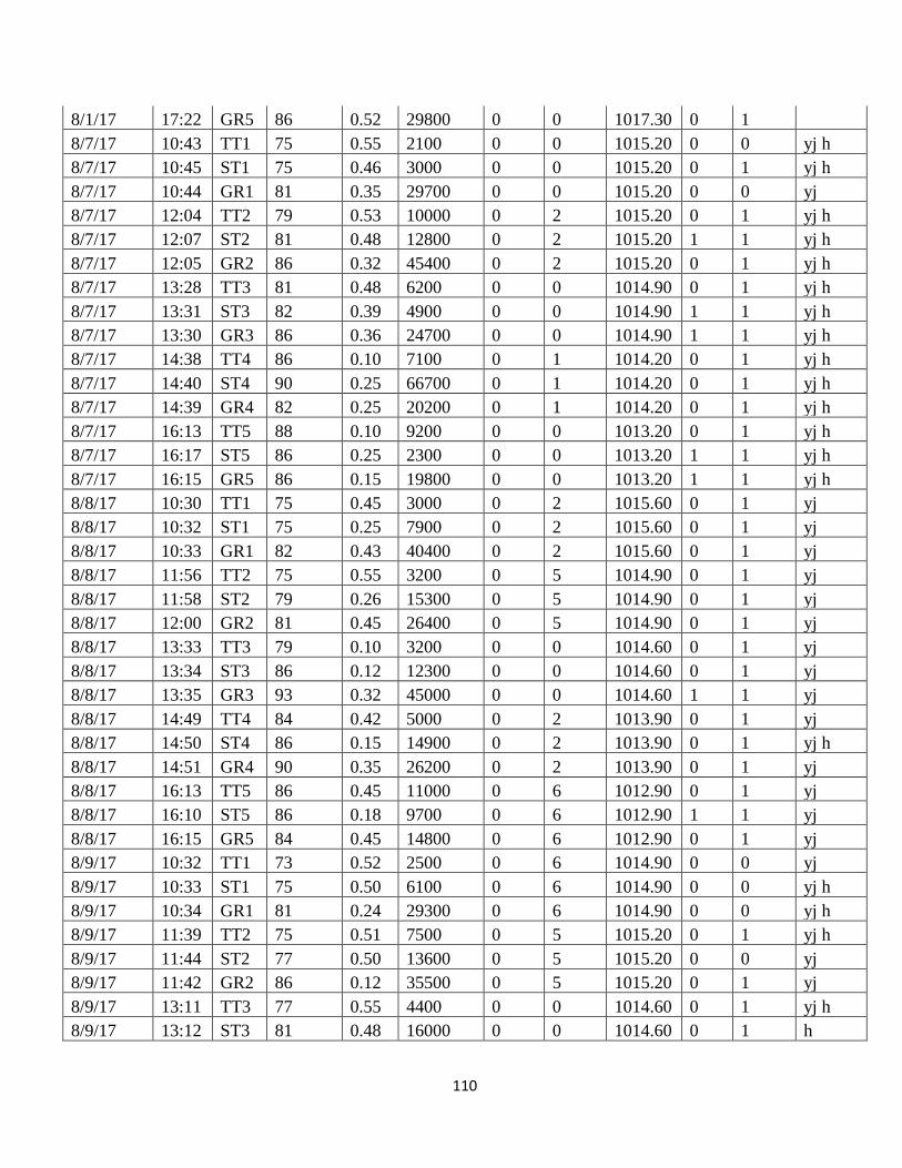
110

8/1/17 17:22 GR5 86 0.52 29800 0 0 1017.30 0 1

8/7/17 10:43 TT1 75 0.55 2100 0 0 1015.20 0 0 yj h

8/7/17 10:45 ST1 75 0.46 3000 0 0 1015.20 0 1 yj h

8/7/17 10:44 GR1 81 0.35 29700 0 0 1015.20 0 0 yj

8/7/17 12:04 TT2 79 0.53 10000 0 2 1015.20 0 1 yj h

8/7/17 12:07 ST2 81 0.48 12800 0 2 1015.20 1 1 yj h

8/7/17 12:05 GR2 86 0.32 45400 0 2 1015.20 0 1 yj h

8/7/17 13:28 TT3 81 0.48 6200 0 0 1014.90 0 1 yj h

8/7/17 13:31 ST3 82 0.39 4900 0 0 1014.90 1 1 yj h

8/7/17 13:30 GR3 86 0.36 24700 0 0 1014.90 1 1 yj h

8/7/17 14:38 TT4 86 0.10 7100 0 1 1014.20 0 1 yj h

8/7/17 14:40 ST4 90 0.25 66700 0 1 1014.20 0 1 yj h

8/7/17 14:39 GR4 82 0.25 20200 0 1 1014.20 0 1 yj h

8/7/17 16:13 TT5 88 0.10 9200 0 0 1013.20 0 1 yj h

8/7/17 16:17 ST5 86 0.25 2300 0 0 1013.20 1 1 yj h

8/7/17 16:15 GR5 86 0.15 19800 0 0 1013.20 1 1 yj h

8/8/17 10:30 TT1 75 0.45 3000 0 2 1015.60 0 1 yj

8/8/17 10:32 ST1 75 0.25 7900 0 2 1015.60 0 1 yj

8/8/17 10:33 GR1 82 0.43 40400 0 2 1015.60 0 1 yj

8/8/17 11:56 TT2 75 0.55 3200 0 5 1014.90 0 1 yj

8/8/17 11:58 ST2 79 0.26 15300 0 5 1014.90 0 1 yj

8/8/17 12:00 GR2 81 0.45 26400 0 5 1014.90 0 1 yj

8/8/17 13:33 TT3 79 0.10 3200 0 0 1014.60 0 1 yj

8/8/17 13:34 ST3 86 0.12 12300 0 0 1014.60 0 1 yj

8/8/17 13:35 GR3 93 0.32 45000 0 0 1014.60 1 1 yj

8/8/17 14:49 TT4 84 0.42 5000 0 2 1013.90 0 1 yj

8/8/17 14:50 ST4 86 0.15 14900 0 2 1013.90 0 1 yj h

8/8/17 14:51 GR4 90 0.35 26200 0 2 1013.90 0 1 yj

8/8/17 16:13 TT5 86 0.45 11000 0 6 1012.90 0 1 yj

8/8/17 16:10 ST5 86 0.18 9700 0 6 1012.90 1 1 yj

8/8/17 16:15 GR5 84 0.45 14800 0 6 1012.90 0 1 yj

8/9/17 10:32 TT1 73 0.52 2500 0 6 1014.90 0 0 yj

8/9/17 10:33 ST1 75 0.50 6100 0 6 1014.90 0 0 yj h

8/9/17 10:34 GR1 81 0.24 29300 0 6 1014.90 0 0 yj h

8/9/17 11:39 TT2 75 0.51 7500 0 5 1015.20 0 1 yj h

8/9/17 11:44 ST2 77 0.50 13600 0 5 1015.20 0 0 yj

8/9/17 11:42 GR2 86 0.12 35500 0 5 1015.20 0 1 yj

8/9/17 13:11 TT3 77 0.55 4400 0 0 1014.60 0 1 yj h

8/9/17 13:12 ST3 81 0.48 16000 0 0 1014.60 0 1 h

111

8/9/17 13:13 GR3 90 0.32 100300 0 0 1014.60 0 1 yj

8/9/17 14:30 TT4 79 0.55 4000 0 0 1014.60 0 1 h

8/9/17 14:31 ST4 81 0.45 9800 0 0 1014.60 0 1 yj

8/9/17 14:32 GR4 91 0.09 24600 0 0 1014.60 0 1 yj

8/9/17 15:51 TT5 81 0.43 4900 0 0 1013.90 0 1 h

8/9/17 15:53 ST5 84 0.50 11100 0 0 1013.90 1 1

8/9/17 15:52 GR5 86 0.20 15600 0 0 1013.90 0 1 yj h

8/23/17 10:47 ST1 68 0.66 3500 0 5 1015.60 0 1 yj

8/23/17 10:48 GR1 75 0.40 18400 0 5 1015.60 0 1 yj

8/23/17 12:20 TT2 75 0.55 1600 0 1 1014.60 0 1 yj h

8/23/17 12:21 ST2 75 0.57 6100 0 1 1014.60 0 1 yj h

8/23/17 12:23 GR2 75 0.40 18000 0 1 1014.60 0 1 yj

8/23/17 13:27 TT3 79 0.51 4400 0 4 1013.90 0 1 yj

8/23/17 13:29 ST3 75 0.55 6000 0 4 1013.90 0 1 yj

8/23/17 13:31 GR3 68 0.31 60300 0 4 1013.90 0 1 yj

8/23/17 14:36 TT4 82 0.45 3000 0 4 1013.50 0 1 yj h

8/23/17 14:37 ST4 77 0.50 3600 0 4 1013.50 0 1 yj

8/23/17 14:38 GR4 82 0.25 15700 0 4 1013.50 0 1 yj h

8/23/17 15:39 TT5 84 0.45 15700 0 4 1012.90 0 1 yj h

8/23/17 15:41 ST5 79 0.50 5700 0 4 1012.90 0 1 yj

8/23/17 15:42 GR5 82 0.25 11500 0 4 1012.90 0 1 yj h

8/25/17 10:44 TT1 61 0.37 800 0 4 1017.30 0 1 yj

8/25/17 10:45 ST1 59 0.59 1800 0 4 1017.30 0 1 yj

8/25/17 10:46 GR1 68 0.46 59900 0 4 1017.30 0 1 yj h

8/25/17 12:19 TT2 66 0.32 1000 0 4 1016.90 0 1 yj

8/25/17 12:20 ST2 68 0.51 7100 0 4 1016.90 0 1 yj

8/25/17 12:21 GR2 64 0.52 6300 0 4 1016.90 0 1 yj

8/25/17 13:46 TT3 72 0.22 1300 0 8 1016.60 0 1 yj g

8/25/17 13:48 ST3 68 0.48 3100 0 8 1016.60 0 1 yj

8/25/17 13:49 GR3 81 0.30 86900 0 8 1016.60 0 1 yj

8/25/17 14:43 TT4 79 0.22 10200 0 7 1016.30 0 1 yj

8/25/17 14:45 ST4 72 0.40 5800 0 7 1016.30 0 1 yj h

8/25/17 14:47 GR4 75 0.28 25900 0 7 1016.30 0 1 yj h

8/25/17 15:30 TT5 73 0.15 16300 0 7 1015.60 0 1 yj h

8/25/17 15:32 ST5 72 0.44 16400 0 7 1015.60 0 1 yj h

8/25/17 15:34 GR5 73 0.10 23100 0 7 1015.60 0 1 yj

8/28/17 11:36 TT1 68 0.62 1300 0 0 1017.60 0 0 yj

8/28/17 11:37 ST1 72 0.42 7800 0 0 1017.60 0 0 yj

8/28/17 11:38 GR1 75 0.52 23400 0 0 1017.60 0 0 yj

112

8/28/17 13:08 TT2 75 0.52 3200 0 0 1016.60 0 1 yj h

8/28/17 13:11 ST2 77 0.30 9100 0 0 1016.60 0 1 yj h

8/28/17 13:12 GR2 84 0.41 47400 0 0 1016.60 0 1 yj h

8/28/17 14:13 TT3 77 0.52 3400 0 0 1015.90 0 1 yj h

8/28/17 14:14 ST3 79 0.33 9600 0 0 1015.90 0 1 yj h

8/28/17 14:15 GR3 82 0.50 24500 0 0 1015.90 0 1 yj h

8/28/17 15:23 TT4 75 0.55 1100 0 0 1014.90 0 1 yj h

8/28/17 15:24 ST4 77 0.35 7300 0 0 1014.90 0 1 yj h

8/28/17 15:25 GR4 97 0.58 14700 0 0 1014.90 0 1 yj h

8/28/17 16:37 TT5 77 0.55 1300 0 0 1014.20 0 1 yj

8/28/17 16:38 ST5 79 0.28 5800 0 0 1014.20 0 1 yj

8/28/17 16:39 GR5 79 0.54 8400 0 0 1014.20 0 1 yj

8/30/17 10:44 TT1 70 0.62 2300 0 0 1011.50 0 1 yj h

8/30/17 10:45 ST1 72 0.42 6700 0 0 1011.50 0 1 yj h

8/30/17 10:46 GR1 75 0.54 35000 0 0 1011.50 0 1 yj

8/30/17 12:06 TT2 79 0.52 2300 0 0 1011.20 0 1 yj h

8/30/17 12:07 ST2 79 0.32 8600 0 0 1011.20 0 1 yj h

8/30/17 12:08 GR2 79 0.51 19800 0 0 1011.20 0 1 yj h

8/30/17 13:42 TT3 81 0.44 5600 0 0 1010.80 0 1 yj h

8/30/17 13:43 ST3 79 0.22 6900 0 0 1010.80 0 1 yj h

8/30/17 13:44 GR3 90 0.43 80600 0 0 1010.80 0 1 yj h

8/30/17 14:52 TT4 86 0.10 5800 0 1 1010.20 0 1 yj h

8/30/17 14:53 ST4 82 0.24 6600 0 1 1010.20 0 1 yj h

8/30/17 14:54 GR4 88 0.41 34900 0 1 1010.20 0 1 yj h

8/30/17 16:14 TT5 86 0.36 19900 0 0 1009.10 0 1 yj h

8/30/17 16;15 ST5 86 0.19 24800 0 0 1009.10 0 1 yj h

8/30/17 16:16 GR5 82 0.43 9100 0 0 1009.10 0 1 yj

9/5/17 11:22 TT1 70 0.49 1800 0 3 1020.00 0 0 yj h

9/5/17 11:23 ST1 72 0.50 8400 0 3 1020.00 0 1

9/5/17 11:24 GR1 72 0.29 13700 0 3 1020.00 0 0 yj

9/5/17 12:37 TT2 72 0.48 1200 0 7 1019.30 0 1 yj

9/5/17 12:38 ST2 75 0.48 8300 0 7 1019.30 0 1 yj

9/5/17 12:39 GR2 75 0.26 14100 0 7 1019.30 0 1 yj

9/5/17 14:13 TT3 75 0.45 1800 0 3 1018.60 0 1 yj

9/5/17 14:15 ST3 77 0.43 10300 0 3 1018.60 0 1 yj

9/5/17 14:16 GR3 79 0.19 17300 0 3 1018.60 0 1 yj

9/5/17 15:12 TT4 75 0.50 2100 0 4 1018.30 0 1 yj

9/5/17 15:13 ST4 75 0.49 7300 0 4 1018.30 0 1 yj

9/5/17 15:14 GR4 79 0.24 11000 0 4 1018.30 0 1 yj

113

9/5/17 16:48 TT5 75 0.54 1000 0 3 1017.60 0 1 yj

9/5/17 16:49 ST5 75 0.50 4100 0 3 1017.60 0 1 yj

9/5/17 16:50 GR5 75 0.36 8500 0 3 1017.60 0 1 yj

10/2/17 10:49 TT1 48 0.70 1700 0 2 1019.00 0 0

10/2/17 10:50 ST1 50 0.72 3600 0 2 1019.00 0 0

10/2/17 10:51 GR1 50 0.53 12900 0 2 1019.00 0 1

10/2/17 12:13 TT2 54 0.70 1200 0 4 1019.60 0 0

10/2/17 12:14 ST2 54 0.66 11000 0 4 1019.60 0 0 yj

10/2/17 12:15 GR2 54 0.50 21200 0 4 1019.60 0 1

10/2/17 14:45 TT3 45 0.88 100 0.07 3 1019.30 0 0 rain

10/2/17 14:46 ST3 45 0.89 100 0.07 3 1019.30 0 0 rain

10/2/17 14:47 GR3 45 0.90 100 0.07 3 1019.30 0 0 rain

10/2/17 15:23 TT4 46 0.90 1700 0.02 2 1020.30 0 0 rain

10/2/17 15:24 ST4 46 0.93 10000 0.02 2 1020.30 0 0 rain

10/2/17 15:25 GR4 50 0.57 12900 0.02 2 1020.30 0 0 rain

10/2/17 16:30 TT5 45 0.85 100 0 4 1020.00 0 0

10/2/17 16:31 ST5 43 0.92 1100 0 4 1020.00 0 0

10/2/17 16:32 GR5 45 0.61 4800 0 4 1020.00 0 0

114

Appendix D

Estimating Probability of Blow Fly Colonization in Eastern ...

Documents

Transcript of Estimating Probability of Blow Fly Colonization in Eastern ...