WORKING PAPER SERIES: NO. 2009-2

Estimating primary demand for substitutable productsfrom sales transaction data

Gustavo Vulcano,

New York University

Garrett J. van Ryzin,

Columbia University

Richard Ratliff,

Sabre Holdings

2009

http://www.cprm.columbia.edu

Estimating primary demand for substitutable products

from sales transaction data

Gustavo Vulcano ∗ Garrett van Ryzin † Richard Ratliff ‡

Original version: July 2008. Revisions: May and December 2009.

Abstract

We consider a method for estimating substitute and lost demand when only sales andproduct availability data are observable, not all products are available in all periods (e.g.,due to stock-outs or availability controls imposed by the seller), and the seller knows itsmarket share. The model combines a multinomial logit (MNL) choice model with a non-homogeneous Poisson model of arrivals over multiple periods. Our key idea is to view theproblem in terms of primary (or first-choice) demand; that is, the demand that would havebeen observed if all products were available in all periods. We then apply the expectation-maximization (EM) method to this model, and treat the observed demand as an incompleteobservation of primary demand. This leads to an efficient, iterative procedure for estimatingthe parameters of the model, which provably converges to a stationary point of the incompletedata log-likelihood function. Every iteration of the algorithm consists of simple, closed-formcalculations. We illustrate the procedure on simulated data and two industry data sets.

Key words: Demand estimation, demand untruncation, choice behavior, multinomial logitmodel, EM method.

∗Leonard N. Stern School of Business, New York University, New York, NY 10012, gvulcano@stern.nyu.edu.†Graduate School of Business, Columbia University, New York, NY 10027, gjv1@columbia.edu.‡Sabre Holdings, Southlake, Texas 76092, Richard.Ratliff@sabre-holdings.com.

1

1 Introduction

Two important problems in retail demand forecasting are estimating turned away demand whenitems are sold out and properly accounting for substitution effects among related items. Forsimplicity, most retail demand forecasts rely on time-series models of observed sales data, whichtreat each stock keeping unit (SKU) as receiving an independent stream of requests. However,if the demand lost when a customer’s first choice is unavailable (referred to as spilled demand)is ignored, the resulting demand forecasts may be negatively biased; this underestimation canbe severe if products are unavailable for long periods of time. Additionally, if products are un-available, stockout-based substitution will lead to increased sales in substitute products which areavailable (referred to as recaptured demand); ignoring recapture in demand forecasting leads toan overestimation bias among the set of available SKUs. Correcting for both spill and recaptureeffects is important in order to establish a good estimate of the true underlying demand forproducts.

A similar problem arises in forecasting demand for booking classes in the airline industry.A heuristic to correct for spilled demand, implemented in many airline revenue managementsystems, is to assume that the percentage of demand turned away is proportional to the degreeof “closedness” of a product (an itinerary-fare-class combination).1 But this can lead to a“double counting” problem, whereby spill is estimated on unavailable products but also countedas recapture on alternate, available products. Empirical studies of different industries show thatstockout-based substitution is a common occurrence: For airline passengers, recapture rates areacknowledged to be in the range of 15%-55% (e.g., Ja et al. [17]), while Gruen et al. [15] reportrecapture rates of 45% across eight categories at retailers worldwide.

While spilled and recaptured demand are not directly observable from sales transactions, var-ious statistical techniques have been proposed to estimate them. Collectively these techniquesare known as demand untruncation or uncensoring methods. One of the most popular suchmethods is the expectation-maximization (EM) algorithm. EM procedures ordinarily employiterative methods to estimate the underlying parameters of interest; in our case, demand bySKU across a set of historical data. The EM method works using alternating steps of computingconditional expected values of the parameter estimates to obtain an expected log-likelihood func-tion (the “E-step”) and maximizing this function to obtain improved estimates (the “M-step”).Traditionally, retail forecasts that employ the EM approach have been limited to untruncatingsales history for individual SKUs and disregard recapture effects from substitute products.

Classical economic theory on substitution effects (e.g., see Nicholson [25]) provides techniquesfor estimating demand shifts due to changes in prices of alternative offerings. However, animportant practical problem is how to fit such demand models when products are out of stockor otherwise unavailable, and do so using only readily-available data, which in most retail settings

1For instance, if a booking class is open during 10 days of a month, and 20 bookings are observed, then this

heuristic approach will estimate a demand of 20× 30/10 = 60 for this booking class.

2

consists of sales transactions, product attributes (brand, size, price, etc.) and on-hand inventoryquantities by SKU. Our work helps address this problem.

A convenient and widely used approach for estimating demand for different SKUs withina set of similar items is to use discrete choice models, such as the multinomial logit (MNL)(e.g., see Ben-Akiva and Lerman [3] and Train [29]). Choice models predict the likelihood ofcustomers purchasing a specific product from a set of related products based on their relativeattractiveness. A convenient aspect of these models is that the likelihood of purchase can bereadily recalculated if the mix of available related products changes (e.g., due to another itembeing sold out or restocked).

In this paper, we propose a novel method of integrating customer choice models with theEM method to untruncate demand and correct for spill and recapture effects across an entire setof related product sales history. The only required inputs are observed historical sales, productavailability data, and market share information. The key idea is to view the problem in terms ofprimary (or first-choice) demand, and to treat the observed sales as incomplete observations ofprimary demand. We then apply the EM method to this primary demand model and show thatit leads to an efficient, iterative procedure for estimating the parameters of the choice modelwhich provably converges to a stationary point of the associated incomplete data log-likelihoodfunction. Our EM method also provides an estimate of the number of lost sales – that is, thenumber of customers who would have purchased if all products were in stock – which is criticalinformation in retailing. The approach is also remarkably simple, practical and effective, asillustrated on simulated data and two industry data sets.

2 Literature review

There are related papers in the revenue management literature on similar estimation problems.Talluri and van Ryzin [28, Section 5] develop an EM method to jointly estimate arrival ratesand parameters of a MNL choice model based on consumer level panel data under unobservableno-purchases. Vulcano et al. [31] provide empirical evidence of the potential of that approach.Ratliff et al. [26] provide a comprehensive review of the demand untruncation literature in thecontext of revenue management settings. They also propose a heuristic to jointly estimate spilland recapture across numerous flight classes, by using balance equations that generalize theproposal of Anderson [1]. A similar approach was presented before by Ja et al. [17].

Another related stream of research is the estimation of demand and substitution effects forassortment planning in retailing. Kok and Fisher [19] identify two common models of substitu-tion:

1. The utility-based model of substitution, where consumers associate a utility with eachproduct (and also with the no-purchase option), and choose the highest utility alternativeavailable. The MNL model belongs to such class. The single period assortment planning

3

problem studied by van Ryzin and Mahajan [30] is an example of the applicability of thismodel.

2. The exogenous model of substitution, where customers choose from the complete set ofproducts, and if the item they choose is not available, they may accept another variant as asubstitute according to a given substitution probability (e.g. see Netessine and Rudi [23]).

Other papers in the operations and marketing science literature also address the problemof estimating substitution behavior and lost sales. Anupindi et al. [2] present a method forestimating consumer demand when the first choice variant is not available. They assume acontinuous time model of demand and develop an EM method to uncensor times of stock-outsfor a periodic review policy, with the constraint that at most two products stock-out in order tohandle a manageable number of variables. They find maximum likelihood estimates of arrivalrates and substitution probabilities.

Swait and Erdem [27] study the effect of temporal consistency of sales promotions andavailability on consumer choice behavior. The former encompasses variability of prices, displays,and weekly inserts. The latter also influences product utility, because the uncertainty of a SKU’spresence in the store may lead consumers to consider the product less attractive. They solve theestimation problem via simulated maximum likelihood and test it on fabric softener panel data,assuming a variation of the MNL model to explain consumer choice; but there is no demanduncensoring in their approach.

Campo et al. [8] investigate the impact of stockouts on purchase quantities by uncovering thepattern of within-category shifts and by analyzing dynamic effects on incidence, quantity andchoice decisions. They propose a modification of the usual MNL model to allow for more gen-eral switching patterns in stock-out situations, and formulate an iterative likelihood estimationalgorithm. They then suggest a heuristic two-stage tracking procedure to identify stock-outs:in a first stage, they identify potential stockout periods; in stage two, these periods are fur-ther screened using a sales model and an iterative outlier analysis procedure (see Appendix Atherein).

Borle et al. [5] analyze the impact of a large-scale assortment reduction on customer retention.They develop models of consumer purchase behavior at the store and category levels, which areestimated using Markov chain Monte Carlo (MCMC) samplers. Contrary to other findings, theirresults indicate that a reduction in assortment reduces overall store sales, decreasing both salesfrequency and quantity.

Chintagunta and Dube [10] propose an estimation procedure that combines information fromhousehold panel data and store level data to estimate price elasticities in a model of consumerchoice with normally-distributed random coefficients specification. Their methodology entailsmaximum likelihood estimation (MLE) with instrumental variables regression (IVR) that usesshare information of the different alternatives (including the no-purchase option). Different fromours, their model requires no-purchase store visit information.

4

Kalyanam et al. [18] study the role of each individual item in an assortment, estimating thedemand for each item as well as the impact of the presence of each item on other individualitems and on aggregate category sales. Using a database from a large apparel retailer, includinginformation on item specific out-of-stocks, they use the variation in a category to study theentire category sales impact of the absence of each individual item. Their model allow for flexiblesubstitution patterns (beyond MNL assumptions), but stock-outs are treated in a somewhat adhoc way via simulated data augmentation. The model parameters are estimated in a hierarchicalBayesian framework also through a MCMC sampling algorithm.

Bruno and Vilcassim [6] propose a model that accounts for varying levels of product avail-ability. It uses information on aggregate availability to simulate the potential assortments thatconsumers may face in a given shopping trip. The model parameters are estimated by drawingmultivariate Bernoulli vectors consistent with the observed aggregate level of availability. Theyshow that neglecting the effects of stock-outs leads to substantial biases in estimation.

More recently, Musalem et al. [22] also investigate substitution effects induced by stock-outs. Different from ours, their model allows for partial information on product availability,which could be the case in a periodic review inventory system with infrequent replenishment.However, their estimation algorithm is much more complex and computationally intensive thanours since it combines MCMC with sampling using Bayesian methods.

The aforementioned paper by Kok and Fisher [19] is close to ours. They develop an EMmethod for estimating demand and substitution probabilities under a hierarchical model ofconsumer purchase behavior at a retailer. This consumer behavior model is similar to theone in Campo et al. [8], and is quite standard in the marketing literature; see e.g. Bucklin andGupta [7], and Chintagunta [9]. In their setting, upon arrival, a consumer decides: 1) whether ornot to buy from a subcategory (purchase-incidence), 2) which variant to buy given the purchaseincidence (choice), and 3) how many units to buy (quantity). Product choice is modeled withthe MNL framework. Unlike our aggregate demand setting, they analyze the problem at theindividual consumer level and assume that the number of customers who visit the store butdid not purchase anything is negligible (see Kok and Fisher [19, Section 4.3]). The outcome ofthe estimation procedure is combined with the parameters of the incidence purchase decision,the parameters of the MNL model for the first choice, and the coefficients for the substitutionmatrix. Due to the complexity of the likelihood function, the EM procedure requires the use ofnon-linear optimization techniques in its M-step.

Closest to our work is that of Conlon and Mortimer [11], who develop an EM algorithm toaccount for missing data in a periodic review inventory system under a continuous time modelof demand, where for every period they try to uncensor the fraction of consumers not affectedby stock-outs. They aim to demonstrate how to incorporate data from short term variations inthe choice set to identify substitution patterns, even when the changes to the choice set are notfully observed. A limitation of this work is that the E-step becomes difficult to implement when

5

multiple products are simultaneously stocked-out, since it requires estimating an exponentialnumber of parameters (see Conlon and Mortimer [11, Appendix A.2]).

In summary, there has been a growing field of literature on estimating choice behavior andlost sales in the context of retailing for the last decade. This stream of research also includesprocedures based on the EM method. Our main contribution to the literature in this regard isa remarkably simple procedure that consists of a repeated sequence of closed-form expressions.The algorithm can be readily implemented in any standard procedural computer language, andrequires minimal computational time.

3 Model, estimation and algorithm

3.1 Model description

A set of n substitutable products is sold over T purchase periods, indexed t = 1, 2, . . . , T . Noassumption is made about the order or duration of these purchase periods. For example, apurchase period may be a day and we might have data on purchases over T (non-necessarilyconsecutive) days, or it may be a week and we have purchase observations for T weeks. Periodscould also be of different lengths and the indexing need not be in chronological order.

The only data available for each period are actual purchase transactions (i.e., how many unitswe have sold of each product in each period), and a binary indicator of the availability of eachproduct during the period. (We assume products are either always available or unavailable in aperiod; see discussion below.) The number of customers arriving and making purchase choices ineach period is not known; equivalently, we do not observe the number of no-purchase outcomes ineach period. This is the fundamental incompleteness in the data, and it is a common limitationof transactional sales data in retail settings in which sales transactions and item availability arefrequently the only data available.

The full set of products is denoted N = {1, . . . , n}. We denote the number of purchases ofproduct i observed in period t by zit, and define zt = (z1t, . . . , znt). We will assume that zit ≥ 0for all i, t; that is, we do not consider returns. Let mt =

∑ni=1 zit denote the total number of

observed purchases in period t. We will further assume without loss of generality that for allproduct i, there exists at least one period t such that zit > 0; else, we can drop product i fromthe analysis.

We assume the following underlying model generates these purchase data: The number ofarrivals in each period (i.e., number of customers who make purchase decisions) is denoted At.At has a Poisson distribution with mean λt (the arrival rate). Let λ = (λ1, . . . , λT ) denote thevector of arrival rates. It may be that some of the n products are not available in certain periodsdue to temporary stock-outs, limited capacity or controls on availability (e.g., capacity controlsfrom a revenue management system, or deliberate scarcity introduced by the seller). Hence,let St ⊂ N denote the set of products available for sale in period t. We assume St is known

6

for each t and that the products in St are available throughout period t. Whenever i 6∈ St, fornotational convenience we define the number of purchases to be zero, i.e., zit = 0.

Customers choose among the alternatives in St according to a MNL model, which is assumedto be the same in each period (i.e., preferences are time homogeneous, though this assumptioncan be relaxed as discussed below). Under the MNL model, the choice probability of a customeris defined based on a preference vector v ∈ Rn, v > 0, that indicates the customer “preferenceweights” or “attractiveness” for the different products.2 This vector, together with a normalized,no-purchase preference weight v0 = 1, determine a customer’s choice probabilities as follows: letPj(S, v) denote the probability that a customer chooses product j ∈ S when S is offered andpreference weights are given by vector v. Then,

Pj(S, v) =vj∑

i∈S vi + 1. (1)

If j 6∈ S, then Pj(S, v) = 0.We denote the no-purchase probability by P0(S, v). It accounts for the fact that when set S

is offered, a customer may either buy a product from a competitor, or not buy at all (i.e., buysthe outside alternative):

P0(S, v) =1∑

i∈S vi + 1.

The no-purchase option can be treated as a separate product (labeled zero) that is alwaysavailable. Note that by total probability,

∑j∈S Pj(S, v) + P0(S, v) = 1.

The statistical challenge we address is how to estimate the parameters of this model – namely,the preference vector v and the arrival rates λ – from the purchase data zt, t = 1, 2, . . . , T .

3.2 The incomplete data likelihood function

One can attempt to solve directly this estimation problem using maximum likelihood estimation(MLE). The incomplete data likelihood function can be expressed as follows:

LI(v,λ) =T∏

t=1

P(mt customers buy in period t|v,λ)

mt!z1t!z2t! · · · znt!

∏

j∈St

[Pj(St,v)∑

i∈StPi(St, v)

]zjt (2)

where the probabilities in the inner product are the conditional probabilities of purchasingproduct j given that a customer purchases something. The number of customers that purchasein period t, mt, is a realization of a Poisson random variable with mean λt

∑i∈St

Pi(St, v), viz

P(mt customers buy in period t|v, λ) =

[λt

∑i∈St

Pi(St, v)]mt e−λt

∑i∈St

Pi(St,v)

mt!. (3)

One could take the log of (2) and attempt to maximize this log-likelihood function withrespect to v and λ. However, it is clear that this is a complex likelihood function without much

2A further generalization of this MNL model to the case where the preference weights are functions of the

product attributes is provided in Section 6.2.

7

structure, so maximizing it (or its logarithm) directly is not an appealing approach. Indeed, ourattempts in this regard were not promising (see Section 5).

3.3 Multiple optima in the MLE and market potential

A further complication is that one can show that the likelihood function (2) has a continuum ofmaxima. To see this, let (v∗, λ∗) denote a maximizer of (2). Let α > 0 be any real number anddefine a new preference vector v0 = αv∗. Define new arrival rates

λ0t =

α∑

i∈Stv∗i + 1

α(∑

i∈Stv∗i + 1

)λ∗t .

Then, it is not hard to see from (1) that

λ∗t Pj(St, v∗) = λ0

t Pj(St, v0),

for all j and t. Since this product of the arrival rate and purchase probability is unchanged, byinspection of the form of (2) and (3), the solution (v0,λ0) has the same likelihood and thereforeis also a maximum. Since this holds true for any α > 0, there are a continuum of maxima.3

One can resolve this multiplicity of optimal solutions by imposing an additional constrainton the parameter values related to market share. Specifically, suppose we have an exogenousestimate of the preference weight of the outside alternative relative to the total set of offerings.Let’s call it r, so that

r :=1∑n

j=1 vj. (4)

Then fixing the value of r resolves the degree of freedom in the multiple maxima. Still, thisleaves the need to solve a complicated optimization problem. In Section 3.5 we look at a simplerand more efficient approach based on viewing the problem in terms of primary – or first-choice– demand.

3.4 Discussion of the model

Our model uses the well-studied MNL for modeling customer choice behavior in a homogeneousmarket (i.e., customer preferences are described by a single set of parameters v). As mentioned,a convenient property of the MNL is that the likelihood of purchase can be readily recalculatedif the availability of the products changes. But the MNL has significant restrictions in termsof modeling choice behavior, most importantly the property of independence from irrelevantalternatives (IIA). Briefly, the property is that that the ratio of purchase probabilities for twoalternatives is constant regardless of the consideration set containing them. Other choice modelsare more flexible in modeling substitution patterns (e.g., see Train [29, Chapter 4]). Among

3Of course, this observation holds more generally: For any pair of values (v, λ), there is a continuum of values

α(v, λ), α > 0, such that LI(v, λ) = LI(αv, αλ).

8

them, the nested logit (NL) model has been widely used in the marketing literature. While lessrestrictive, the NL requires more parameters and therefore a higher volume of data to generategood estimates.

Despite the limitation of the IIA property, MNL models are widely used. Starting withGuadagni and Little [16], marketing researchers have found that the MNL model works quitewell when estimating demand for a category of substitutable products (in Guadagni and Little’sstudy, regular ground coffee of different brands). Recent experience in the airline industry alsoprovides good support for using the MNL model.4 According to the experience of one of theauthors, there are two major considerations in real airline implementations: (i) the range offare types included, and (ii) the flight departure time proximity. Regarding (i), in cases whereairlines are dealing with dramatically different fare products, then it is often better to splitthe estimation process using two entirely separate data pools. Consider the following real-worldexample: an international airline uses the first four booking classes in their nested fare hierarchyfor international point-of-sales fares which have traditional restrictions (i.e., advance purchase,minimum stay length, etc); these are the highest-valued fare types. The next eight bookingclasses are used for domestic travel with restriction-free fares. Because there is little (or no)interaction between the international and domestic points-of-sales, the airline applies the MNLmodel to two different data pools: one for international sales and the other for domestic sales.Separate choice models are fit to the two different pools. Regarding (ii), it would be somewhatunrealistic to assume that first-choice demand for a closed 7am departure would be recapturedonto a same day, open 7pm departure in accordance with the IIA principle. Hence, it makessense to restrict the choice set to departure times that are more similar. Clearly some customerswill refuse to consider the alternative flight if the difference in departure times is large. Somerecently developed revenue management systems with which the authors are familiar still usethe MNL for such flight sets, but they implement a correction heuristic to overcome the IIAlimitation.

Another important consideration in our model is the interpretation of the outside alternative,and the resulting interpretation of the arrival rates λ. For instance, if the outside alternative isassumed to be the (best) competitor’s product, then

s = 1/(1 + r) =

∑nj=1 vj∑n

j=1 vj + 1

defines the retailer’s market share, and λ refers to the volume of purchases in the market,including the retailer under consideration and its competitor(s). Alternatively, if the outsidealternative is considered to consist of both the competitor’s best product and a no-purchaseoption, then s gives the retailer’s “market potential”, and λ is then interpreted as the totalmarket size (number of customers choosing). This later interpretation is found in marketing

4For example, Sabre has been implementing the single-segment MNL model for a large domestic US airline for

more than two years, and has been observing very significant revenue improvements.

9

and empirical industrial organizations applications (e.g., see Berry et al. [4] for an empiricalstudy of the U.S. automobile industry, and Nevo [24] for an empirical study of the ready-to-eatcereal industry). Henceforth, given an indicator s (share or potential), we set the attractivenessof the outside alternative as r = (1 − s)/s, which is equivalent to (4). Low values of r implyhigher participation in the market.

Also, note we work with store-level data (as opposed to household panel data). Chintaguntaand Dube [10] discuss the advantages of using store-level data to compute the mean utilityassociated with products.

We also assume that for every product j, there is a period t for which zjt > 0 (otherwise,that product can be dropped from the analysis). In this regard, our model can accommodateassortments with slow moving items for which zjt = 0 for several (though that all) periods. It’sworth noting that for retail settings, having zero sales in many consecutive periods could bea symptom of inventory record error. DeHoratius and Raman [12] found that 65% of 370,000inventory records of a large public U.S. retailer were inaccurate, and that the magnitude of theinaccuracies was significant (of around 35% of the inventory level on the shelf per SKU). Apossible misleading situation is that the IT system records a SKU as being in-stock even thoughthere are no units on the shelf, and hence no sales will be observed despite the fact that theproduct is tagged as “available”.

Further, if a period t has no sales for any of the products, then that period can be droppedfrom the analysis – or equivalently, it can be established ex-ante that all primary demands Xjt

and substitute demands Yjt, j = 1, . . . , n, as well as the arrival rate λt will be zero. This isbecause our model assumes that the market participation s is replicated in every single period,and hence no sale in a period is a signal of no arrival in that period.

Regarding the information on product availability, as mentioned above we assume that aproduct is either fully available or not available throughout a given period t. Hence, the timepartitioning should be fine enough to capture short-term changes in the product availabilityover time. However, in contrast to other approaches (e.g., Musalem et al. [22]), we do notrequire information on inventory levels; all we require is a binary indicator describing eachitem’s availability.

Finally, note that our model assumes homogeneous preferences across the whole selling hori-zon, but a non-homogeneous Poisson arrival process of consumers. The assumption of homo-geneous preferences can be relaxed by splitting the data into intervals where a different choicemodel is assumed to apply over each period. The resulting modification is straightforward, sowe do not elaborate on this extension. The estimates λ can be used to build a forecast ofthe volume of demand to come by applying standard time series analysis to project the valuesforward in time.

10

3.5 Log-likelihood based on primary demand

By primary (or first-choice) demand for product i, we mean the demand that would have occurredfor product i if all n alternatives were available. The (random) number of purchases, Zit, ofproduct i in period t may be greater than the primary demand because it could include purchasesfrom customers whose first choice was not available and bought product i as a substitute (i.e., Zit

includes demand that is spilled from other unavailable products and recaptured by product i).More precisely, the purchase quantity Zit can be split into two components: the primary demand,Xit, which is the number of customers in period t that have product i as their first choice; andYit, the substitute demand, which is the number of customers in period t that decide to buyproduct i as a substitute because their first choice is unavailable. Thus:

Zit = Xit + Yit. (5)

We focus on estimating the primary demand Xit. While this decomposition seems to introducemore complexity in the estimation problem, we show below that in fact leads to a considerablysimpler estimation algorithm.

3.5.1 Basic identities

Let Xjt = E[Xjt|zt] and Yjt = E[Yjt|zt] denote, respectively, the conditional expectation of theprimary and substitute demand given the purchase observations zt. We seek to determine thesequantities.

Consider first products that are unavailable in period t, that is j 6∈ St⋃{0}. For these items,

we have no observation zjt. To determine Xjt for these items, note that

E[Xjt|zt] =vj∑n

i=1 vi + 1E[At|zt]

and ∑

h∈St

E [Zht|zt] =

∑h∈St

vh∑h∈St

vh + 1E[At|zt].

Combining these expressions to eliminate E[At|zt] yields

E[Xjt|zt] =vj∑n

i=1 vi + 1

∑h∈St

vh + 1∑h∈St

vh

∑

h∈St

E [Zht|zt] ,

or equivalently,

Xjt =vj∑n

i=1 vi + 1

∑h∈St

vh + 1∑h∈St

vh

∑

h∈St

zht, j 6∈ St

⋃{0}. (6)

Next consider the available products j ∈ St. For each such product, we have zjt observedtransactions which according to (5) can be split into

zjt = Xjt + Yjt, j ∈ St.

11

Note that

P{Product j is a first choice|Purchase j} =P{Product j is a first choice}

P{Purchase j}

=vj∑n

i=1 vi + 1

/vj∑

h∈Stvh + 1

=

∑h∈St

vh + 1∑ni=1 vi + 1

.

Therefore, since Xjt = zjtP{Product j is a first choice|Purchase j}, we have

Xjt =

∑h∈St

vh + 1∑ni=1 vi + 1

zjt, and Yjt =

∑h6∈St

⋃{0} vh∑ni=1 vi + 1

zjt. (7)

Lastly, for the no-purchase option (i.e., j = 0), we are also interested in estimating itsprimary demand in period t conditional on the transaction data, i.e., X0t = E[X0t|zt]. Recallthat At is the total (random) number of arrivals in period t, including the customers that donot purchase. Again, we do not observe At directly but note that

E[X0t|zt] =1∑n

i=1 vi + 1E[At|zt]. (8)

In addition, the following identity should hold:

At = X0t +n∑

i=1

Xit.

Conditioning on the observed purchases we have that

E[At|zt] = X0t +n∑

i=1

Xit. (9)

Substituting (9) into (8), we obtain:

X0t =1∑n

i=1 vi

n∑

i=1

Xit. (10)

Interestingly, we can also get the lost sales in period t, given by the conditional expectation ofthe substitute demand for the no-purchase option, Y0t = E[Y0t|zt]:

Y0t =1∑

i∈Stvi + 1

∑

h6∈St⋃{0}

Xht.

Next, define Nj , j = 0, . . . , n, as the total primary demand for product j over all periods(including the no-purchase option j = 0). Thus, Nj =

∑Tt=1 Xjt, giving an estimate

Nj :=T∑

t=1

Xjt, (11)

where, consistent with our other notation, Nj = E[Nj |z1, . . . ,zT ], which is positive becauseXjt ≥ 0, for all j and t, and for at least one period t, Xjt > 0.5

5This is due to our assumption that v > 0, and that for at least one period t, zjt > 0, for each j = 1, . . . , n.

12

3.5.2 Overview of our approach

The key idea behind our approach is to view the problem of estimating v and λ as an estimationproblem with incomplete observations of the primary demand Xjt, j = 0, 1, . . . , n, t = 1, . . . , T .Indeed, suppose we had complete observations of the primary demand. Then the log-likelihoodfunction would be quite simple, namely

L(v) =n∑

j=1

Nj ln(

vj∑ni=1 vi + 1

)+ N0 ln

(1∑n

i=1 vi + 1

),

where Nj is the total number of customers selecting product j as their first choice (or selectingnot to purchase, j = 0, as their first choice). We show below this function has a closed-form maximum. However, since we don’t observe Nj , j = 0, 1, . . . , n, directly, we use the EMmethod of Dempster et al. [13] to estimate the model. This approach drastically simplifies thecomputational problem relative to maximizing (2). It also has the advantage of eliminating λ

from the estimation problem and reducing it to a problem in v only. (An estimate of λ can betrivially recovered after the algorithm runs as discussed below.)

The EM method is an iterative procedure that consists of two steps per iteration: an ex-pectation (E) step and a maximization (M) step. Starting from arbitrary initial estimates ofthe parameters, it computes the conditional expected value of the log-likelihood function withrespect to these estimates (the E-step), and then maximizes the resulting expected log-likelihoodfunction to generate new estimates (the M-step). The procedure is repeated until convergence.While technical convergence problems can arise, in practice the EM method is a robust andefficient way to compute maximum likelihood estimates for incomplete data problems.

In our case, the method works by starting with estimates v > 0 (the E-step). These estimatesfor the preference weights are used to compute estimates for the total primary demand valuesN0, N1, . . . , Nn, by using the formulas in (6), (7), and (10), and then substituting the values ofXjt in (11). In the M-step, given estimates v (and therefore, given estimates for N0, N1, . . . , Nn),we then maximize the conditional expected value of the log-likelihood function with respect tov:

E[L(v)|v] =n∑

j=1

Nj ln(

vj∑ni=1 vi + 1

)+ N0 ln

(1∑n

i=1 vi + 1

). (12)

Just as in the likelihood function (2), there is a degree of freedom in our revised estimationformulation. Indeed, consider the first iteration with arbitrary initial values for the estimates v,yielding estimates Nj , j = 0, 1, . . . , n. From (10), r defined in (4) must satisfy N0 = r

∑nj=1 Nj .

As above, r measures the magnitude of outside alternative demand relative to the alternativesin N . We will prove later in Proposition 1 that this relationship is preserved across differentiterations of the EM method. So the initial guess for v implies an estimate of r.

13

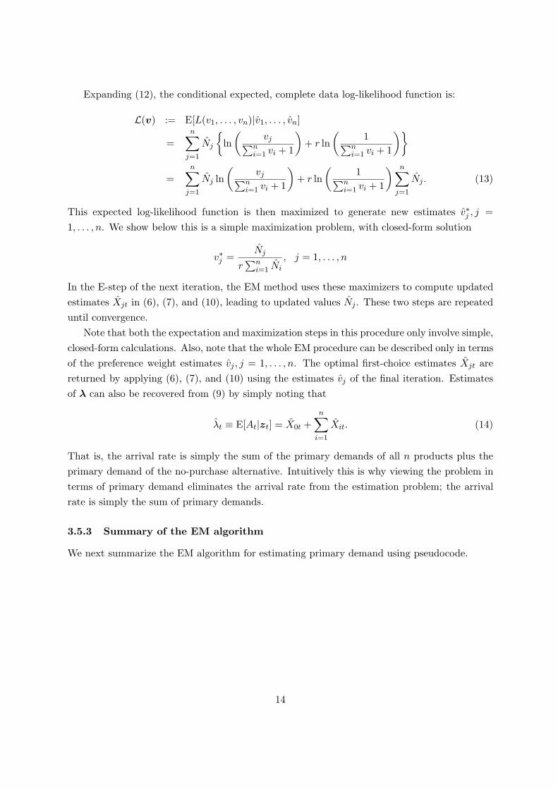
Expanding (12), the conditional expected, complete data log-likelihood function is:

L(v) := E[L(v1, . . . , vn)|v1, . . . , vn]

=n∑

j=1

Nj

{ln

(vj∑n

i=1 vi + 1

)+ r ln

(1∑n

i=1 vi + 1

)}

=n∑

j=1

Nj ln(

vj∑ni=1 vi + 1

)+ r ln

(1∑n

i=1 vi + 1

) n∑

j=1

Nj . (13)

This expected log-likelihood function is then maximized to generate new estimates v∗j , j =1, . . . , n. We show below this is a simple maximization problem, with closed-form solution

v∗j =Nj

r∑n

i=1 Ni

, j = 1, . . . , n

In the E-step of the next iteration, the EM method uses these maximizers to compute updatedestimates Xjt in (6), (7), and (10), leading to updated values Nj . These two steps are repeateduntil convergence.

Note that both the expectation and maximization steps in this procedure only involve simple,closed-form calculations. Also, note that the whole EM procedure can be described only in termsof the preference weight estimates vj , j = 1, . . . , n. The optimal first-choice estimates Xjt arereturned by applying (6), (7), and (10) using the estimates vj of the final iteration. Estimatesof λ can also be recovered from (9) by simply noting that

λt ≡ E[At|zt] = X0t +n∑

i=1

Xit. (14)

That is, the arrival rate is simply the sum of the primary demands of all n products plus theprimary demand of the no-purchase alternative. Intuitively this is why viewing the problem interms of primary demand eliminates the arrival rate from the estimation problem; the arrivalrate is simply the sum of primary demands.

3.5.3 Summary of the EM algorithm

We next summarize the EM algorithm for estimating primary demand using pseudocode.

14

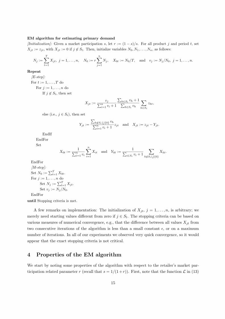
EM algorithm for estimating primary demand[Initialization]: Given a market participation s, let r := (1 − s)/s. For all product j and period t, setXjt := zjt, with Xjt := 0 if j 6∈ St. Then, initialize variables N0, N1, . . . , Nn, as follows:

Nj :=T∑

t=1

Xjt, j = 1, . . . , n, N0 := r

n∑

j=1

Nj , X0t := N0/T, and vj := Nj/N0, j = 1, . . . , n.

Repeat[E-step]:For t := 1, . . . , T do

For j := 1, . . . , n doIf j 6∈ St, then set

Xjt :=vj∑n

i=1 vi + 1

∑h∈St

vh + 1∑h∈St

vh

∑

h∈St

zht,

else (i.e., j ∈ St), then set

Yjt :=

∑h6∈St

⋃{0} vh∑ni=1 vi + 1

zjt and Xjt := zjt − Yjt.

EndIfEndForSet

X0t :=1∑n

i=1 vi

n∑

i=1

Xit and Y0t :=1∑

i∈Stvi + 1

∑

h6∈St

⋃{0}Xht.

EndFor[M-step]:Set N0 :=

∑Tt=1 X0t.

For j := 1, . . . , n doSet Nj :=

∑Tt=1 Xjt.

Set vj := Nj/N0.EndFor

until Stopping criteria is met.

A few remarks on implementation: The initialization of Xjt, j = 1, . . . , n, is arbitrary; wemerely need starting values different from zero if j ∈ St. The stopping criteria can be based onvarious measures of numerical convergence, e.g., that the difference between all values Xjt fromtwo consecutive iterations of the algorithm is less than a small constant ε, or on a maximumnumber of iterations. In all of our experiments we observed very quick convergence, so it wouldappear that the exact stopping criteria is not critical.

4 Properties of the EM algorithm

We start by noting some properties of the algorithm with respect to the retailer’s market par-ticipation related parameter r (recall that s = 1/(1+ r)). First, note that the function L in (13)

15

is linearly decreasing as a function of r, for all r > 0. Second, as claimed above, the value r

remains constant throughout the execution of the algorithm:

Proposition 1 The relationship N0 = r∑n

j=1 Nj, is preserved across iterations of the EMalgorithm, starting from the initial value of r.

Proof. In the E-step of an iteration, after we compute the values Xit, we use formula (10) withthe vjs replaced by the optimal values obtained in the M-step of the previous iteration, i.e.,

X0t =1

∑ni=1

N ′i

r∑n

h=1 N ′h

n∑

i=1

Xit = rn∑

i=1

Xit,

where N ′i stand for the volume estimates from the previous iteration. The new no-purchase

estimate is

N0 =T∑

t=1

X0t =T∑

t=1

rn∑

i=1

Xit

= rn∑

i=1

T∑

t=1

Xit = rn∑

i=1

Ni,

and hence the relationship N0 = r∑n

j=1 Nj , is preserved.

Our next result proves that the complete data log-likelihood function L(v1, . . . , vn) is indeedunimodal:

Theorem 1 The function L(v1, . . . , vn), with v > 0, and Nj > 0,∀j, is unimodal, with unique

maximizer v∗j = Nj

r∑n

i=1 Ni, j = 1, . . . , n.

Proof. Taking partial derivatives of function (13), we get:

∂

∂vjL(v1, . . . , vn) =

Nj

vj− (1 + r)

∑ni=1 Ni∑n

i=1 vi + 1, j = 1, . . . , n.

Setting these n equations equal to zero leads to a linear system with unique solution:

v∗j =Nj

r∑n

i=1 Ni

, j = 1, . . . , n. (15)

The second cross partial derivatives are:

∂2

∂2vjL(v1, . . . , vn) = −Nj

v2j

+ γ(v1, . . . , vn),

where

γ(v1, . . . , vn) =(1 + r)

∑ni=1 Ni

(∑n

i=1 vi + 1)2,

16

and∂2

∂vj∂viL(v1, . . . , vn) = γ(v1, . . . , vn), j 6= i.

Let H be the Hessian of L(v1, . . . , vn). In order to check that our critical point (15) is a localmaximum, we compute for x ∈ Rn, x 6= 0,

xT H(v1, . . . , vn) x =(1 + r)

(∑ni=1 Ni

)(∑n

i=1 xi)2

(∑n

i=1 vi + 1)2−

n∑

i=1

Nix2

i

v2i

. (16)

The second order sufficient conditions are xT H(v∗1, . . . , v∗n) x < 0, for all x 6= 0. Plugging in the

expressions in (15), we get

xT H(v∗1, . . . , v∗n) x = r2

(n∑

i=1

Ni

)((∑n

i=1 xi)2

1 + r−

(n∑

i=1

Ni

)n∑

i=1

x2i

Ni

).

Note that since r > 0, and Nj > 0, ∀j, it is enough to check that(

n∑

i=1

xi

)2

−(

n∑

i=1

Ni

)n∑

i=1

x2i

Ni

≤ 0, ∀x 6= 0. (17)

By the Cauchy-Schwartz inequality, i.e., |yTz|2 ≤ ||y||2 ||z||2, defining yi = xi√Ni

and zi =√

Ni,we get:

(n∑

i=1

xi

)2

=

(n∑

i=1

xi√Ni

×√

Ni

)2

≤

√√√√n∑

i=1

x2i

Ni

2

√√√√n∑

i=1

Ni

2

=

(n∑

i=1

x2i

Ni

) (n∑

i=1

Ni

),

and therefore inequality (17) holds.Proceeding from first principles, we have a unique critical point for L(v1, . . . , vn) which is a

local maximum. The only other potential maxima can occur at a boundary point. But close tothe boundary of the domain the function is unbounded from below; that is

limvj↓0

L(v1, . . . , vn) = −∞, j = 1, . . . , n.

Hence, the function is unimodal.

A few comments are in order. First, observe that equation (16) also shows that the functionL(v1, . . . , vn) is not jointly concave in general, since there could exist a combination of valuesN1, . . . , Nn, and the vector (v1, . . . , vn) such that for some x, xTH(v1, . . . , vn)x > 0.6 Figure 1illustrates one example where L(v1, . . . , vn) is not concave. Second, due to the definition of v∗j ,

6For example, if we take n = 2, v = (1.5, 1.2), N1 = 50, N2 = 3, and x = (0.01, 1), then r = 1/(v1 +v2) = 0.37,

and xTH(v1, v2)x = 3.33.

17

0

20

40

60

80

100

020

4060

80100

−300

−250

−200

−150

−100

−50

v1

v2

L(v 1,v

2)

Figure 1: Example of log-likelihood function L(v1, v2), for r = 0.02, N1 = 60, and N2 = 50. The maximizer is

v∗ = (27.27, 22.73).

and since∑T

t=1 zjt > 0, then Nj > 0 for every iteration of the EM method. Third, Theorem 1proves that the M-step of the EM procedure is always well defined, and gives a unique globalmaximizer. This means it is indeed an EM algorithm, as opposed to the so-called GeneralizedEM algorithm (GEM). In the case of GEM, the M-step only requires that we generate animproved set of estimates over the current ones7, and the conditions for convergence are morestringent (e.g., see McLachlan and Krishnan [21, Chapter 3] for further discussion.)

The following result shows that the EM method in our case satisfies a regularity conditionthat guarantees convergence of the log-likelihood values of the incomplete-data function to astationary point:

Theorem 2 (Adapted from Wu [32]) 8 The conditional expected value E[L(v1, . . . , vn)|v1, . . . , vn]in (13) is continuous both in v > 0 and v > 0, and hence all the limit points of any in-stance {v(k), λ

(k), k = 1, 2, . . .} of the EM algorithm are stationary points of the corresponding

incomplete-data log-likelihood function LI(v, λ), and LI(v(k), λ(k)

) converges monotonically toa value LI(v∗, λ∗), for some stationary point (v∗,λ∗).

Proof. The result simply follows from the fact that Nj =∑T

t=1 Xjt, j = 0, 1, . . . , n, and Xjt

is continuous in v according to equations (6), (7), and (10). Clearly, L is also continuous in v.In addition, recall that the estimates v imply a vector λ once we fix a market participation r

(through equation (14), and therefore the EM algorithm indeed generates an implied sequence{v(k), λ

(k), k = 1, 2, . . .}.

7In particular, the M-step of GEM just requires to find a vector v such that E[L(v)|v]] ≥ E[L(v)|v]. See

McLachlan and Krishnan [21, Section 1.5.5].8See also McLachlan and Krishnan [21, Theorem 3.2].

18

5 Numerical Examples

We next report on two sets of numerical examples. The first set is based on simulated data,which was used to get a sense of how well the procedure identifies a known demand systemand how much data is necessary to get good estimates. Then, we provide two other examplesbased on real-world data sets, one for airlines and another for retail. In all the examples, weset a stopping criteria based on the difference between the matrices X from two consecutiveiterations of the EM method, and stopped the procedure as soon as the absolute value of allthe elements of the difference matrix was smaller than 0.001. The algorithm was implementedusing the MATLAB9 procedural language, in which the algorithm detailed in Section 3.5.3 isstraightforward to code.

5.1 Examples based on simulated data

Our first example is small and illustrates the behavior of the procedure. We provide the originalgenerated data (observed purchases) and the final data (primary and substitute demands). Next,we look at the effect of data volume and quality on the accuracy of the estimates.

5.1.1 Preliminary estimation case

Given a known underlying MNL choice model (i.e., values for the preference weights v) andassuming that the arrivals follow a homogeneous Poisson process with rate λ = 50, we simulatedpurchases for n = 5 different products. Initially, we considered a selling horizon of T = 15periods, and preference weights v = (1, 0.7, 0.4, 0.2, 0.05) (recall that the weight of the no-purchase alternative is v0 = 1). Note w.l.o.g. we index products in decreasing order of preference.These preference values give a market potential s =

∑nj=1 vj/(

∑nj=1 vj + 1) = 70%.

Table 1 describes the simulated retail data, showing the randomly generated purchases foreach of the five products for each period and total number of no-purchases and arrivals. Here,period 1 represents the end of the selling horizon. Note a label “NA” in position (j, t) meansthat product j is not available in period t. The unavailability was exogenously set prior tosimulating the purchase data.

For the estimation procedure, the initial values of vj are computed following the suggestionin Section 3.5.3, i.e.,

vj =∑T

t=1 zjt

r∑T

t=1

∑ni=1 zit

, j = 1, . . . , n.

We also assume perfect knowledge of the market potential. The output is shown in Table 2.The second column includes the true preference weight values for reference. The third columnreports the estimates computed by the EM method. The fourth column reports the percentagebias between the estimated and true values. Note that the results suggest an apparent bias in

9MATLAB is a trademark of The MathWorks, Inc. We used version 6.5.1 for Microsoft Windows.

19

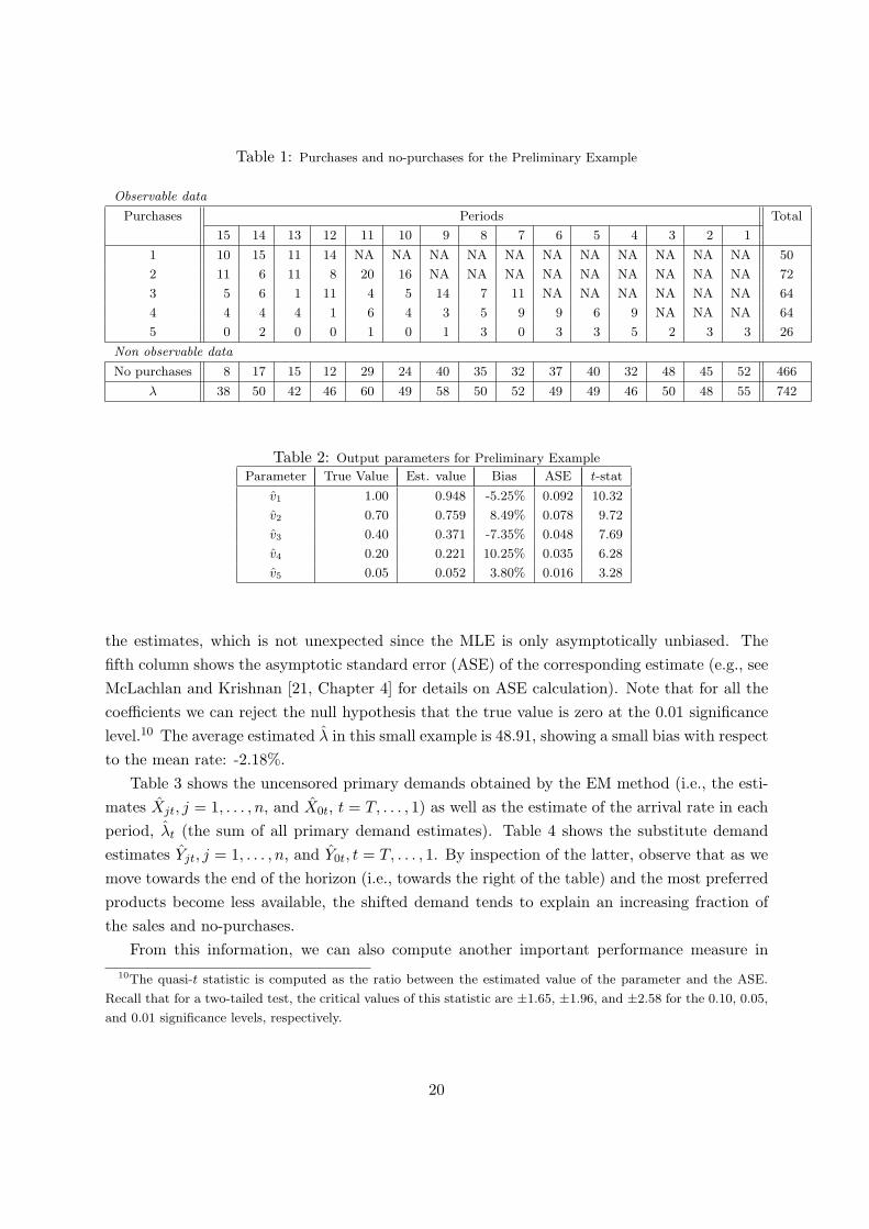
Table 1: Purchases and no-purchases for the Preliminary Example

Observable data

Purchases Periods Total

15 14 13 12 11 10 9 8 7 6 5 4 3 2 1

1 10 15 11 14 NA NA NA NA NA NA NA NA NA NA NA 50

2 11 6 11 8 20 16 NA NA NA NA NA NA NA NA NA 72

3 5 6 1 11 4 5 14 7 11 NA NA NA NA NA NA 64

4 4 4 4 1 6 4 3 5 9 9 6 9 NA NA NA 64

5 0 2 0 0 1 0 1 3 0 3 3 5 2 3 3 26

Non observable data

No purchases 8 17 15 12 29 24 40 35 32 37 40 32 48 45 52 466

λ 38 50 42 46 60 49 58 50 52 49 49 46 50 48 55 742

Table 2: Output parameters for Preliminary Example

Parameter True Value Est. value Bias ASE t-stat

v1 1.00 0.948 -5.25% 0.092 10.32

v2 0.70 0.759 8.49% 0.078 9.72

v3 0.40 0.371 -7.35% 0.048 7.69

v4 0.20 0.221 10.25% 0.035 6.28

v5 0.05 0.052 3.80% 0.016 3.28

the estimates, which is not unexpected since the MLE is only asymptotically unbiased. Thefifth column shows the asymptotic standard error (ASE) of the corresponding estimate (e.g., seeMcLachlan and Krishnan [21, Chapter 4] for details on ASE calculation). Note that for all thecoefficients we can reject the null hypothesis that the true value is zero at the 0.01 significancelevel.10 The average estimated λ in this small example is 48.91, showing a small bias with respectto the mean rate: -2.18%.

Table 3 shows the uncensored primary demands obtained by the EM method (i.e., the esti-mates Xjt, j = 1, . . . , n, and X0t, t = T, . . . , 1) as well as the estimate of the arrival rate in eachperiod, λt (the sum of all primary demand estimates). Table 4 shows the substitute demandestimates Yjt, j = 1, . . . , n, and Y0t, t = T, . . . , 1. By inspection of the latter, observe that as wemove towards the end of the horizon (i.e., towards the right of the table) and the most preferredproducts become less available, the shifted demand tends to explain an increasing fraction ofthe sales and no-purchases.

From this information, we can also compute another important performance measure in10The quasi-t statistic is computed as the ratio between the estimated value of the parameter and the ASE.

Recall that for a two-tailed test, the critical values of this statistic are ±1.65, ±1.96, and ±2.58 for the 0.10, 0.05,

and 0.01 significance levels, respectively.

20

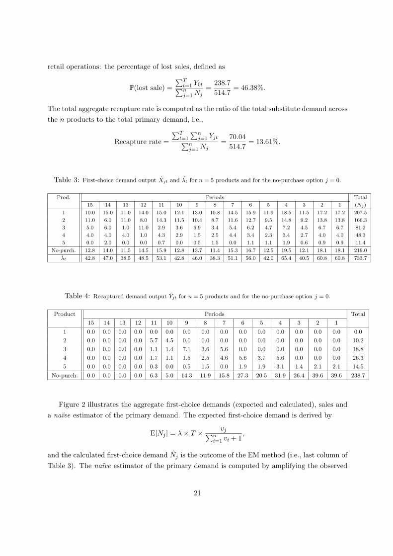
retail operations: the percentage of lost sales, defined as

P(lost sale) =∑T

t=1 Y0t∑nj=1 Nj

=238.7514.7

= 46.38%.

The total aggregate recapture rate is computed as the ratio of the total substitute demand acrossthe n products to the total primary demand, i.e.,

Recapture rate =

∑Tt=1

∑nj=1 Yjt∑n

j=1 Nj=

70.04514.7

= 13.61%.

Table 3: First-choice demand output Xjt and λt for n = 5 products and for the no-purchase option j = 0.

Prod. Periods Total

15 14 13 12 11 10 9 8 7 6 5 4 3 2 1 (Nj)

1 10.0 15.0 11.0 14.0 15.0 12.1 13.0 10.8 14.5 15.9 11.9 18.5 11.5 17.2 17.2 207.5

2 11.0 6.0 11.0 8.0 14.3 11.5 10.4 8.7 11.6 12.7 9.5 14.8 9.2 13.8 13.8 166.3

3 5.0 6.0 1.0 11.0 2.9 3.6 6.9 3.4 5.4 6.2 4.7 7.2 4.5 6.7 6.7 81.2

4 4.0 4.0 4.0 1.0 4.3 2.9 1.5 2.5 4.4 3.4 2.3 3.4 2.7 4.0 4.0 48.3

5 0.0 2.0 0.0 0.0 0.7 0.0 0.5 1.5 0.0 1.1 1.1 1.9 0.6 0.9 0.9 11.4

No-purch. 12.8 14.0 11.5 14.5 15.9 12.8 13.7 11.4 15.3 16.7 12.5 19.5 12.1 18.1 18.1 219.0

λt 42.8 47.0 38.5 48.5 53.1 42.8 46.0 38.3 51.1 56.0 42.0 65.4 40.5 60.8 60.8 733.7

Table 4: Recaptured demand output Yjt for n = 5 products and for the no-purchase option j = 0.

Product Periods Total

15 14 13 12 11 10 9 8 7 6 5 4 3 2 1

1 0.0 0.0 0.0 0.0 0.0 0.0 0.0 0.0 0.0 0.0 0.0 0.0 0.0 0.0 0.0 0.0

2 0.0 0.0 0.0 0.0 5.7 4.5 0.0 0.0 0.0 0.0 0.0 0.0 0.0 0.0 0.0 10.2

3 0.0 0.0 0.0 0.0 1.1 1.4 7.1 3.6 5.6 0.0 0.0 0.0 0.0 0.0 0.0 18.8

4 0.0 0.0 0.0 0.0 1.7 1.1 1.5 2.5 4.6 5.6 3.7 5.6 0.0 0.0 0.0 26.3

5 0.0 0.0 0.0 0.0 0.3 0.0 0.5 1.5 0.0 1.9 1.9 3.1 1.4 2.1 2.1 14.5

No-purch. 0.0 0.0 0.0 0.0 6.3 5.0 14.3 11.9 15.8 27.3 20.5 31.9 26.4 39.6 39.6 238.7

Figure 2 illustrates the aggregate first-choice demands (expected and calculated), sales anda naıve estimator of the primary demand. The expected first-choice demand is derived by

E[Nj ] = λ× T × vj∑ni=1 vi + 1

,

and the calculated first-choice demand Nj is the outcome of the EM method (i.e., last column ofTable 3). The naıve estimator of the primary demand is computed by amplifying the observed

21

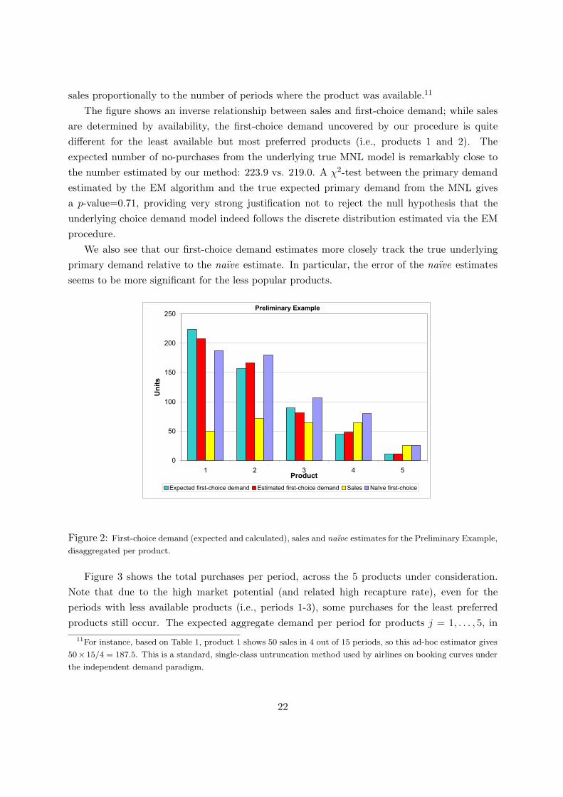
sales proportionally to the number of periods where the product was available.11

The figure shows an inverse relationship between sales and first-choice demand; while salesare determined by availability, the first-choice demand uncovered by our procedure is quitedifferent for the least available but most preferred products (i.e., products 1 and 2). Theexpected number of no-purchases from the underlying true MNL model is remarkably close tothe number estimated by our method: 223.9 vs. 219.0. A χ2-test between the primary demandestimated by the EM algorithm and the true expected primary demand from the MNL givesa p-value=0.71, providing very strong justification not to reject the null hypothesis that theunderlying choice demand model indeed follows the discrete distribution estimated via the EMprocedure.

We also see that our first-choice demand estimates more closely track the true underlyingprimary demand relative to the naıve estimate. In particular, the error of the naıve estimatesseems to be more significant for the less popular products.

Preliminary Example

0

50

100

150

200

250

1 2 3 4 5Product

Un

its

Expected first-choice demand Estimated first-choice demand Sales Naïve first-choice

Figure 2: First-choice demand (expected and calculated), sales and naıve estimates for the Preliminary Example,

disaggregated per product.

Figure 3 shows the total purchases per period, across the 5 products under consideration.Note that due to the high market potential (and related high recapture rate), even for theperiods with less available products (i.e., periods 1-3), some purchases for the least preferredproducts still occur. The expected aggregate demand per period for products j = 1, . . . , 5, in

11For instance, based on Table 1, product 1 shows 50 sales in 4 out of 15 periods, so this ad-hoc estimator gives

50× 15/4 = 187.5. This is a standard, single-class untruncation method used by airlines on booking curves under

the independent demand paradigm.

22

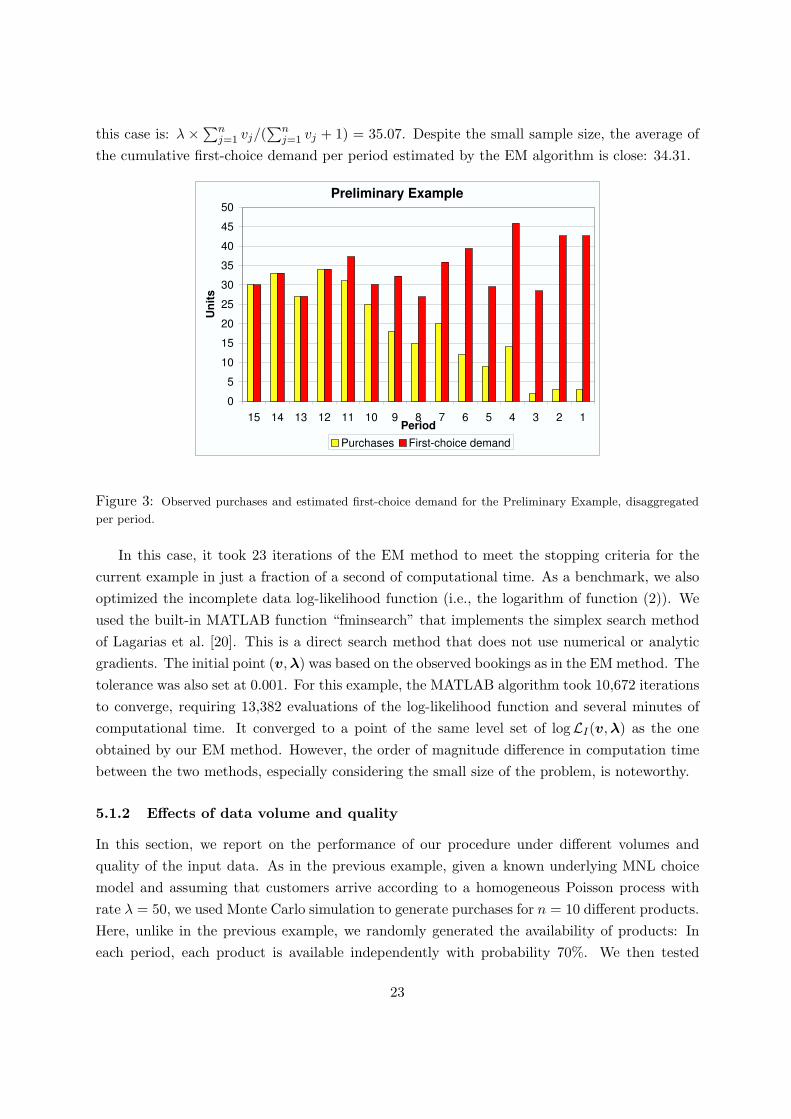
this case is: λ ×∑nj=1 vj/(

∑nj=1 vj + 1) = 35.07. Despite the small sample size, the average of

the cumulative first-choice demand per period estimated by the EM algorithm is close: 34.31.

Preliminary Example

0

5

10

15

20

25

30

35

40

45

50

15 14 13 12 11 10 9 8 7 6 5 4 3 2 1Period

Un

its

Purchases First-choice demand

Figure 3: Observed purchases and estimated first-choice demand for the Preliminary Example, disaggregated

per period.

In this case, it took 23 iterations of the EM method to meet the stopping criteria for thecurrent example in just a fraction of a second of computational time. As a benchmark, we alsooptimized the incomplete data log-likelihood function (i.e., the logarithm of function (2)). Weused the built-in MATLAB function “fminsearch” that implements the simplex search methodof Lagarias et al. [20]. This is a direct search method that does not use numerical or analyticgradients. The initial point (v, λ) was based on the observed bookings as in the EM method. Thetolerance was also set at 0.001. For this example, the MATLAB algorithm took 10,672 iterationsto converge, requiring 13,382 evaluations of the log-likelihood function and several minutes ofcomputational time. It converged to a point of the same level set of logLI(v,λ) as the oneobtained by our EM method. However, the order of magnitude difference in computation timebetween the two methods, especially considering the small size of the problem, is noteworthy.

5.1.2 Effects of data volume and quality

In this section, we report on the performance of our procedure under different volumes andquality of the input data. As in the previous example, given a known underlying MNL choicemodel and assuming that customers arrive according to a homogeneous Poisson process withrate λ = 50, we used Monte Carlo simulation to generate purchases for n = 10 different products.Here, unlike in the previous example, we randomly generated the availability of products: Ineach period, each product is available independently with probability 70%. We then tested

23

various volumes of simulated data, ranging from 10 to 5,000 periods.We further considered three different market potential scenarios: A weak market position

where s = 14%, an intermediate market position where s = 46%, and a dominant position wheres = 81%. Figure 4 shows the box plot of the biases of the estimates v under the different marketpotential conditions. On each box, the central mark is the median, the edges of the box are the25th and 75th percentiles, the whiskers extend to the most extreme data points not consideredoutliers, and outliers are plotted individually. The average of the estimates λt was always veryclose to the mean 50, consistently exhibiting a very small bias compared with the bias for the v

(generally within [-2%, 2%]), and so we did not include it in the box plot.As expected, we note that for each market potential scenario, as we increase the number

of periods, the biases decrease. Having T = 50 periods seem to be enough to get most biasessmaller than 10%. At the same time, as we increase the market potential (and hence, morepurchases per period are observed), we note a trend towards more accuracy with fewer periods.

One potential concern of our procedure is the need to get an exogenous estimate of marketshare and the impact this estimate has on the quality of the estimation. To test this sensitivity,we used the same inputs for generating data as above (i.e., λ = 50, n = 10, products availablewith probability 70%) for the case of T = 500 periods. We then applied our EM procedureassuming inaccurate information about the market potential. Specifically, we perturbed s by±10% and ±20%, and plotted the biases of the estimates v and the average λ (Figure 5, left),and of the estimates of the primary demand Nj , j = 1, . . . , n, and the average λ (Figure 5,right). Note that a perturbation of the market potential generally amplifies the biases of theestimated parameters v and the average λ with respect to their original values. However, thealgorithm adjusts these biases in such a way that it preserves the quality of the estimates of theprimary demand volume for products j = 1, . . . , n. In other words, the relative preferences acrossproducts are sensitive to the initial assumption made about market potential (see Section 6.1for further discussion), yet Figure 5 (right) shows a relatively small bias in the resulting primarydemand estimates.

5.2 Industry data sets

We next present results of two estimation examples based on real-world data sets, one for anairline market and one for a retail market.

5.2.1 Airline Market Example

This example is based on data from a leading commercial airline serving a sample O-D marketwith two daily flights. We present it to illustrate the practical feasibility of our approach andto show the impact of the choice set design on the estimation outcome.

We analyzed bookings data for the last seven selling days prior to departure for each consec-utive Monday from January to March of 2004 (eleven departure days total). There were eleven

24

10 50 100 500 1000 5000-50%

-40%

-30%

-20%

-10%

0%

10%

20%

30%

40%

50%

60%

70%

Bia

s

Number of periods T

10 50 100 500 1000 5000-50%

-40%

-30%

-20%

-10%

0%

10%

20%

30%

40%

50%

60%

70%

Bia

s

Number of periods T

10 50 100 500 1000 5000-50%

-40%

-30%

-20%

-10%

0

10%

20%

30%

40%

50%

60%

70%

Bia

s

Number of periods T

(a) s=14% (b) s=46%

(c) s=81%

Figure 4: Biases of the preference weights v under different market potentials: (a) s = 14%, (b) s = 46%, and

(c) s = 81%, for different selling horizon lengths.

classes per flight, and each class has a different fare value, which were constant during the elevendeparture days under consideration. The market share of the airline for this particular O-D pairwas known to be approximately 50%. As explained in Section 3.3, we use this information as afirst order approximation for the market potential s.

We define a product as a flight-number-class combination, so we had 2× 11 = 22 products.For each product, we had seven booking periods (of length 24 hours) per departure day, leadingto a total of 7× 11 = 77 observation periods. There were non-zero bookings for 15 out of the 22products, so we focused our analysis on these 15 products. We note that in the raw data weoccasionally observed a few small negative values as demand realizations; these negative valuescorresponded to ticket cancelations, and for our analysis we simply set them to zero.

We computed two estimates for the demand volume, under different assumptions: In the

25

multi-flight case we assumed customers chose between both flights in the day, so the choiceset consisted of all 15 products; in the independent-flight case, we assumed customers wereinterested in only one of the two flights, implying there were two disjoint choice sets, one foreach of the flights with 7 and 8 products respectively, and with a market share of 25% per flight.It took 31 iterations of the EM method to compute the multi-flight estimates, and 24 and 176iterations for each of the independent flights. In all cases, the total computational time was onlya few seconds.

Figure 6 shows the observed and predicted bookings, and EM-based and naıve estimates ofthe first-choice demand for the 15 products under consideration, for the multi-flight case. Thepredicted bookings are computed based on the EM estimates v and λ, and on the availabilityinformation of the different products:

E[Bookings of product j on day t] = λtvjI{j ∈ St}∑

i∈Stvi + 1

. (18)

The label in the horizontal axis represent the fares of the corresponding products (e.g., “F1, $189”means “Flight 1, bucket with fare $189”). Figure 7 shows similar statistics for the independentflight case. While the total number of bookings observed is 337, the total estimated volumefor the first-choice demand of the 15 products is 613 for the multi-flight case and 1,597 for theindependent-flight case. As one might expect, the most significant mismatches occur at the lowfares, where price sensitive customers could either buy-up, buy from a competitor, or not buyat all. Note that the procedure leads to significantly different volume estimates for some of thealternatives (e.g., product “F2, $279” has a primary demand of 128 units for the multi-flightcase and 735 units for the independent-flight case). Comparing the two cases, the multi-flightcase has more degrees of freedom in fitting the product demands because it includes relativeattractiveness across more options. The significant differences between the two approachessuggests that the definition of choice set can have a profound impact on the demand volumeestimates. Hence, how best to construct these sets is an important area of future research (e.g.,see Fitzsimons [14] for an analysis of the impact of choice set design on stockouts).

Figure 8 shows the preference weights v = (v1, . . . , v15) computed for both the multi-flightand the independent flight cases via the EM and the naıve methods. Even though there aredifferences between the preference weights derived under both choice set definitions, these dif-ferences are not as extreme as the difference in the first-choice demand volume estimates.

Using the estimates Y0t and Nj , we then computed the fraction of lost sales. For the multi-flight case the estimate was 42.4%, and for the two-independent flight case, the estimates are33.1% and 86.1% for each flight, respectively. In addition, for the multi-flight case, in Figure 9we plot the fraction of lost sales as a fraction of the number of unavailable products. Thisfraction is almost linearly increasing in the number of stocked-out products.12

12This pattern is different from the one observed by Musalem et al. [22] for a mass consumer good (shampoo

in their case), for which the increase is exponential.

26

We conducted two in-sample tests to check the goodness-of-fit of our estimation procedure. 13

First, we ran our estimation procedure to generate v and λ. Then, using information on theavailability of each product across the 77 periods, we estimated the number of bookings perperiod. We aggregated these expected bookings at the weekly level, producing a 15× 11 grid ofestimated bookings. The resulting root mean square error (RMSE) for the multi-flight case was5.10. For both independent flight cases, the RMSEs were 5.82 and 2.90, respectively.

Next, we aggregated the observed bookings and the expected bookings across all the 77 pe-riods and ran a χ2-test for the multi-flight case (giving a p-value=0.72) and for the independentflight cases (with both p-values=0.99), giving strong justification not to reject the null hypoth-esis that the observed bookings follow the distribution estimated via the EM procedure.14 Theaccuracy measures obtained suggest that considering both flights separately seems to betterexplain the choice behavior of customers.

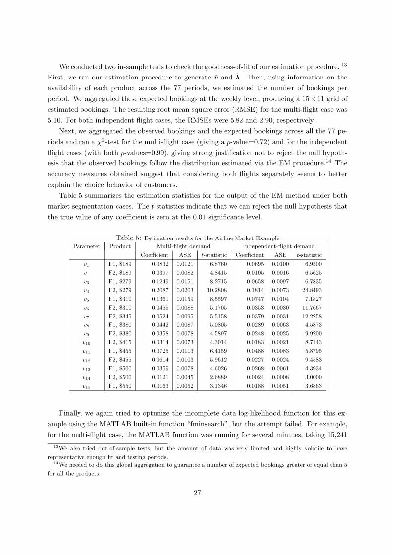
Table 5 summarizes the estimation statistics for the output of the EM method under bothmarket segmentation cases. The t-statistics indicate that we can reject the null hypothesis thatthe true value of any coefficient is zero at the 0.01 significance level.

Table 5: Estimation results for the Airline Market Example

Parameter Product Multi-flight demand Independent-flight demand

Coefficient ASE t-statistic Coefficient ASE t-statistic

v1 F1, $189 0.0832 0.0121 6.8760 0.0695 0.0100 6.9500

v1 F2, $189 0.0397 0.0082 4.8415 0.0105 0.0016 6.5625

v3 F1, $279 0.1249 0.0151 8.2715 0.0658 0.0097 6.7835

v4 F2, $279 0.2087 0.0203 10.2808 0.1814 0.0073 24.8493

v5 F1, $310 0.1361 0.0159 8.5597 0.0747 0.0104 7.1827

v6 F2, $310 0.0455 0.0088 5.1705 0.0353 0.0030 11.7667

v7 F2, $345 0.0524 0.0095 5.5158 0.0379 0.0031 12.2258

v8 F1, $380 0.0442 0.0087 5.0805 0.0289 0.0063 4.5873

v9 F2, $380 0.0358 0.0078 4.5897 0.0248 0.0025 9.9200

v10 F2, $415 0.0314 0.0073 4.3014 0.0183 0.0021 8.7143

v11 F1, $455 0.0725 0.0113 6.4159 0.0488 0.0083 5.8795

v12 F2, $455 0.0614 0.0103 5.9612 0.0227 0.0024 9.4583

v13 F1, $500 0.0359 0.0078 4.6026 0.0268 0.0061 4.3934

v14 F2, $500 0.0121 0.0045 2.6889 0.0024 0.0008 3.0000

v15 F1, $550 0.0163 0.0052 3.1346 0.0188 0.0051 3.6863

Finally, we again tried to optimize the incomplete data log-likelihood function for this ex-ample using the MATLAB built-in function “fminsearch”, but the attempt failed. For example,for the multi-flight case, the MATLAB function was running for several minutes, taking 15,241

13We also tried out-of-sample tests, but the amount of data was very limited and highly volatile to have

representative enough fit and testing periods.14We needed to do this global aggregation to guarantee a number of expected bookings greater or equal than 5

for all the products.

27

iterations and 17,980 evaluations of the function logLI(v, λ), but it converged to a meaning-less point involving negative arrival rates. While one could attempt to stabilize this procedureand come up with better starting points, the experience attests to the simplicity, efficiency androbustness of our method relative to brute-force MLE.

5.2.2 Retail Market Example

This next example illustrates our methodology applied to sales data from a retail chain. Weconsider sales observed during eight weeks over a sample selling season. We assume a uniquechoice set defined by 6 substitutable products within the same small subcategory of SKUs. Themarket share of this retail location is estimated to be 48%. In this example, it took 120 iterationsof the EM method to reach convergence; again, the computation time was a few seconds at most.

Figure 10 shows the observed sales, the predicted sales based on the EM estimates, the EM-based primary demand, and the naıve primary demand for the 6 products under consideration.While the total number of observed sales was 93, the total estimated volume of first-choicedemand for these products was 303. The observed and estimated sales seem to be quite close. Infact, a χ2-test between the observed and estimated sales volume gives a p-value=0.97, providingvery strong evidence not to reject the null hypothesis that the observed bookings follow thedistribution estimated via the EM method. For this example, we observe a major discrepancybetween the primary demands computed via EM and those computed via the naıve approach,much more so than in the airline market example.

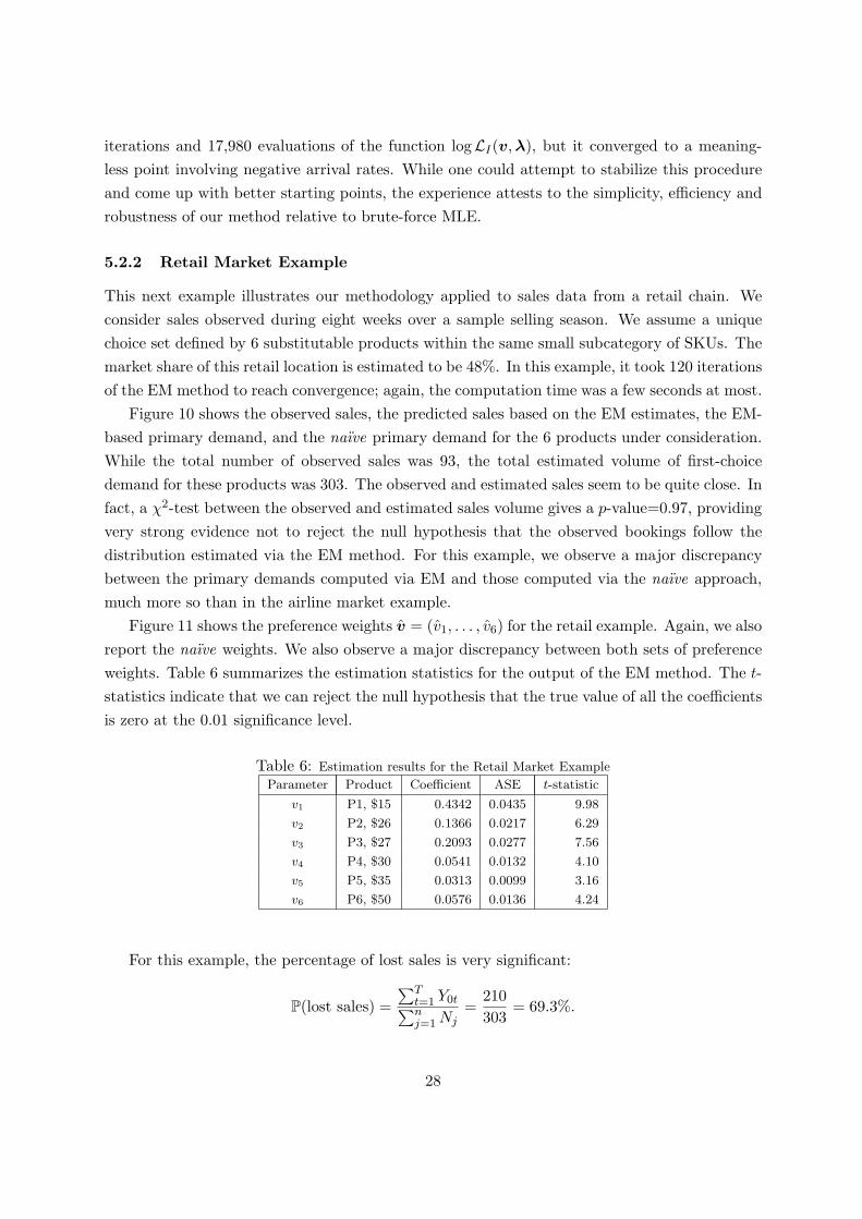
Figure 11 shows the preference weights v = (v1, . . . , v6) for the retail example. Again, we alsoreport the naıve weights. We also observe a major discrepancy between both sets of preferenceweights. Table 6 summarizes the estimation statistics for the output of the EM method. The t-statistics indicate that we can reject the null hypothesis that the true value of all the coefficientsis zero at the 0.01 significance level.

Table 6: Estimation results for the Retail Market Example

Parameter Product Coefficient ASE t-statistic

v1 P1, $15 0.4342 0.0435 9.98

v2 P2, $26 0.1366 0.0217 6.29

v3 P3, $27 0.2093 0.0277 7.56

v4 P4, $30 0.0541 0.0132 4.10

v5 P5, $35 0.0313 0.0099 3.16

v6 P6, $50 0.0576 0.0136 4.24

For this example, the percentage of lost sales is very significant:

P(lost sales) =∑T

t=1 Y0t∑nj=1 Nj

=210303

= 69.3%.

28

Finally, when applying the MATLAB built-in function “fminsearch” to optimize the log-likelihood function for this example, the attempt failed once again. The MATLAB function ranfor several minutes, taking 5,304 iterations and 6,809 evaluations of the function logLI(v, λ),but it converged to a point with several negative arrival rates.

6 Implementation issues and extensions

6.1 Model inputs

While the overall procedure as stated above is quite simple and efficient, there are severalpractical issues that warrant further discussion. One issue we observed is that the estimates aresensitive to how choice sets are defined. Hence, it is important to have a good understanding ofthe set of products that customers consider and to test these different assumptions.

We have also noticed that with some data sets, the method can lead to extreme estimates,for example arrival rates that tend to infinity or preference values that tend to zero. This is nota fault of the algorithm per se, but rather the maximum likelihood criterion. In these cases, wehave found it helpful to impose various ad hoc bounding rules to keep the parameter estimateswithin a plausible range. In markets where the seller has significant market power, we havefound it reasonable to set a value s no larger than 90%. Otherwise, our experience is that weget abnormally high recapture rates into the least preferred products.

Lastly, there is the issue of obtaining a good estimate of the market share or market po-tential s (recall that this depends on our interpretation of the outside alternative). In ei-ther case, note that this share is based on an implicit “all-open” product offering, i.e., s =∑n

i=1 vi/(∑n

i=1 vi +1). This is a difficult quantity to measure empirically in some environments,and indeed our entire premise is that products may not be available in every period.

Nevertheless, the following procedure avoids estimating an “all open”-based s: Recall fromSection 3.3 that given MLE estimates v∗ and λ∗, we can scale this estimate by an arbitraryconstant α > 0 to obtain a new MLE of the form

v(α) = αv∗

λ(α) =α

∑i∈St

v∗i + 1α

(∑i∈St

v∗i + 1)λ∗.

The family of MLE estimates v(α),λ(α) all lead to the same expected primary demand for theown products j = 1, . . . , n for all α, but they produce different expected numbers of customerswho choose the outside alternative (i.e., buy a competitor’s product or do not buy at all).Therefore, if we have a measure of actual market share over the same time periods from othersources (based on actual availability rather than on the “all open” assumption), one can simplysearch for a value of α that produces a total expected market share (using (18)) that matchesthe total observed market share. This is a simple one-dimensional, closed-form search since thefamily of MLE’s v(α), λ(α) is a closed-form function of α.

29

6.2 Linear-in-parameters utility

In our basic setting, we focus on estimating a vector of preference weights v. A common formof the MNL model assumes the preference weight vj can be further broken down into a functionof attributes of the form vj = euj where uj = βT xj is the mean utility of alternative j, xj is avector of attributes of alternative j, and β is a vector of coefficients (part worths) that assign autility to each attribute. Expressed this way, the problem is one of estimating the coefficients β.

Our general primary demand approach is still suitable for this MNL case. The only differenceis that now there is no closed-form solution for the M-step of the EM algorithm, and onemust resort to nonlinear optimization packages to solve for the optimal β in each iteration.Alternatively, one could try the following heuristic approach. The vector of coefficients β couldbe computed in a two-phase approach: In step 1, we run the EM algorithm as described here toestimate v. In step 2 we can look for a vector β that best matches these values using the factthat vj = euj = βT xj , j = 1, . . . , n. In most cases, this will be an over-determined system ofequations, in which case we could a run least squares regression to fit β.

7 Conclusions

Estimating the underlying demand for products when there are significant substitution effectsand lost sales is a common problem in many retail markets. In this paper, we propose a method-ology for estimating demand when the seller knows her market share, only sales transaction dataand product availability data are available, and the assortment changes from period to period.

Our approach combines a multinomial logit (MNL) demand model with a non-homogeneousPoisson model of arrivals over multiple periods. The problem we address is how to jointlyestimate the parameters of this combined model; i.e., preference weights of the products, andarrival rates. Our key idea is to view the problem in terms of primary demand, and to treat theobserved sales as incomplete observations of primary demand. We then apply the expectation-maximization (EM) method to this incomplete demand model, and show that this leads toa very simple, highly efficient iterative procedure for estimating the parameters of the modelwhich provably converges to a stationary point of the incomplete data log-likelihood function.We provide numerical examples that illustrate the applicability of the approach on two industrydata sets.

The methodology is very computationally efficient and simple to implement. In our expe-rience, when applied over large volumes of data, our algorithm runs an order of magnitudefaster than directly optimizing the corresponding incomplete data log-likelihood function (as-suming that a maximum is found for the latter, which in our experience is not always feasiblewith standard optimization routines). Given its simplicity to implement, the realistic input dataneeded, and the quality of the results, we believe that our EM algorithm has significant practicalpotential.

30

Acknowledgements

We would like to thank John Blankenbaker at Sabre Holdings for his careful review and construc-tive suggestions on earlier drafts of this work, in particular his important finding that showedthe existence of a continuum of maxima in the absence of a market potential parameter. RossDarrow and Ben Vinod at Sabre Holdings also provided helpful comments on our work. Finally,we thank Marcelo Olivares (Columbia University), the associate editor, and three anonymousreferees for their constructive feedback.

References

[1] S.E. Andersson. Passenger choice analysis for seat capacity control: A pilot project in Scan-dinavian Airlines. International Transactions in Operational Research, 5:471–486, 1998.

[2] R. Anupindi, M. Dada, and S. Gupta. Estimation of consumer demand with stock-out basedsubstitution: An application to vending machine products. Marketing Science, 17:406–423,1998.

[3] M. Ben-Akiva and S. Lerman. Discrete Choice Analysis: Theory and Applications to TravelDemand. The MIT Press, Cambridge, MA, sixth edition, 1994.

[4] S. Berry, J. Levinsohn, and A. Pakes. Automobile prices in market equilibrium. Economet-rica, 63:841–890, 1995.

[5] S. Borle, P. Boatwright, J. Kadane, J. Nunes, and S. Galit. The effect of product assortmentchanges on customer retention. Marketing Science, 24:616–622, 2005.

[6] H. Bruno and N. Vilcassim. Structural demand estimation with varying product availability.Marketing Science, 27:1126–1131, 2008.

[7] R. Bucklin and S. Gupta. Brand choice, purchase incidence, and segmentation: An inte-grated modeling approach. Journal of Marketing Research, 29:201–215, 1992.

[8] K. Campo, E. Gijsbrechts, and P. Nisol. The impact of retailer stockouts on wether, howmuch, and what to buy. International Journal of Research in Marketing, 20:273–286, 2003.

[9] P. Chintagunta. Investigating purchase incidence, brand choice and purchase quantitydecisions on households. Marketing Science, 12:184–208, 1993.

[10] P. Chintagunta and J-P Dube. Estimating a SKU-level brand choice model that combineshousehold panel data and store data. Journal of Marketing Research, 42:368–379, 2005.

[11] C. Conlon and J. Mortimer. Demand estimation under incomplete product availability.Working paper, Department of Economics, Harvard University, Cambridge, MA, 2009.

31

[12] N. DeHoratius and A. Raman. Inventory record inaccuracy: An empirical analysis. Man-agement Science, 54:627–641, 2008.

[13] A. Dempster, N. Laird, and D. Rubin. Maximum likelihood from incomplete data via theEM algorithm. Journal of the Royal Statistical Society B, 39:1–38, 1977.

[14] G. Fitzsimons. Consumer response to stockouts. Journal of Consumer Research, 27:249–266, 2000.

[15] T. Gruen, D. Corsten, and S. Bharadwaj. Retail out-of-stocks: A worldwide examinationof causes, rates, and consumer responses. Grocery Manufacturers of America, 2002.

[16] P. Guadagni and J. Little. A logit model of brand choice calibrated on scanner data.Marketing Science, 2:203–238, 1983.

[17] S. Ja, B. V. Rao, and S. Chandler. Passenger recapture estimation in airline revenuemanagement. In AGIFORS 41st Annual Symposium, Sydney, Australia, August 2001.Presentation.

[18] K. Kalyanam, S. Borle, and P. Boatwright. Deconstructing each item’s category contribu-tion. Marketing Science, 26:327–341, 2007.

[19] G. Kok and M. Fisher. Demand estimation and assortment optimization under substitution:Methodology and application. Operations Research, 55:1001–1021, 2007.

[20] J. Lagarias, J. Reeds, M. Wright, and P. Wright. Convergence properties of the Nelder-Meadsimplex method in low dimensions. SIAM Journal of Optimization, 9:112–147, 1998.

[21] G. McLachlan and T. Krishnan. The EM Algorithm and Extensions. John Wiley & Sons,New York, NY, 1996.

[22] A. Musalem, M. Olivares, E. Bradlow, C. Terwiesch, and D. Corsten. Structural estimationof the effect of out-of-stocks. Working paper, Fuqua School of Business, Duke University,Durham, NC, 2009.

[23] S. Netessine and N. Rudi. Centralized and competitive inventory models with demandsubstitution. Operations Research, 51:329–335, 2003.

[24] A. Nevo. Measuring market power in the ready-to-eat cereal industry. Econometrica,69:307–342, 2001.

[25] W. Nicholson. Microeconomic Theory: Basic Principles and Extensions. The Dryden Press,5th edition, 1992.

32

[26] R. Ratliff, B. Rao, C. Narayan, and K. Yellepeddi. A multi-flight recapture heuristic forestimating unconstrained demand from airline bookings. Journal of Revenue and PricingManagement, 7:153–171, 2008.

[27] J. Swait and T. Erdem. The effects of temporal consistency of sales promotions and avail-ability on consumer choice behavior. Journal of Marketing Research, 39:304–320, 2002.

[28] K. T. Talluri and G. J. van Ryzin. Revenue management under a general discrete choicemodel of consumer behavior. Management Science, 50:15–33, 2004.

[29] K. Train. Discrete choice methods with simulation. Cambridge University Press, New York,NY, 2003.

[30] G. van Ryzin and S. Mahajan. On the relationships between inventory costs and varietybenefits in retail assortments. Management Science, 45:1496–1509, 1999.

[31] G. Vulcano, G. van Ryzin, and W. Chaar. Choice-based revenue management: An empiricalstudy of estimation and optimization. Leonard N. Stern School of Business, New YorkUniversity, New York, NY. Forthcoming in M&SOM, 2009.

[32] C.F. Wu. On the convergence properties of the EM algorithm. The Annals of Statistics,11:95–103, 1983.

33

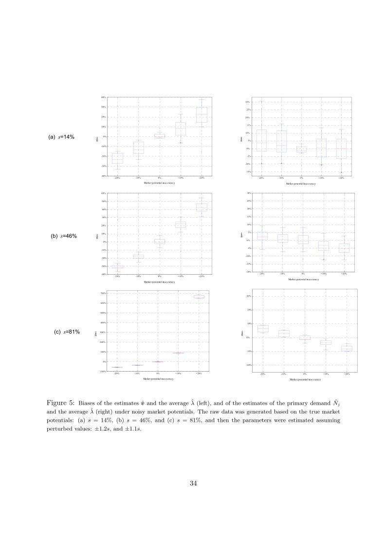
-20% -10% 0% +10% +20%-40%

-30%

-20%

-10%

0%

10%

20%

30%

40%

Bias

Market potential inaccuracy

-20% -10% 0% +10% +20%-40%

-30%

-20%

-10%

0%

10%

20%

30%

40%

50%

60%

Bias

Market potential inaccuracy

(a) s=14%

(b) s=46%

(c) s=81%

-20% -10% 0% +10% +20%

-15%

-10%

-5%

0%

5%

10%

15%

20%

25%

30%

Bias

Market potential inaccuracy

-20% -10% 0% +10% +20%-20%

-15%

-10%

-5%

0%

5%

10%

15%

20%

25%

30%

Bias

Market potential inaccuracy

-20% -10% 0% +10% +20%

-20%

-10%

0%

10%

20%

30%

Bias

Market potential inaccuracy

-20% -10% 0% +10% +20%-100%

0%

100%

200%

300%

400%

500%

600%

700%

Bias

Market potential inaccuracy

Figure 5: Biases of the estimates v and the average λ (left), and of the estimates of the primary demand Nj

and the average λ (right) under noisy market potentials. The raw data was generated based on the true market

potentials: (a) s = 14%, (b) s = 46%, and (c) s = 81%, and then the parameters were estimated assuming

perturbed values: ±1.2s, and ±1.1s.

34

Airline market example: Joint estimation

0

20

40

60

80

100

120

140

F1, $189 F2, $189 F1, $279 F2, $279 F1, $310 F2, $310 F2, $345 F1, $380 F2, $380 F2, $415 F1, $455 F2, $455 F1, $500 F2, $500 F1, $550

Product

Un

its

Observed bookings Predicted bookings EM-based primary demand Naïve primary demand

Figure 6: Comparison of observed and predicted bookings, EM-based and naıve first-choice demand under the

multi-flight assumption for the Airline Market Example.

735

Figure 7: Comparison of observed and predicted bookings, EM-based and naıve first-choice demand under the

independent flight assumption for the Airline Market Example.

35

Airline market example

0.00

0.05

0.10

0.15

0.20

0.25

F1,$189

F2,$189

F1,$279

F2,$279

F1,$310

F2,$310

F2,$345

F1,$380

F2,$380

F2,$415

F1,$455

F2,$455

F1,$500

F2,$500

F1,$550

Preference weight v

Naïve multi-flight Naïve indep. flights EM-based multi-flight EM-based indep. flights

Figure 8: Comparison of EM-based and naıve preference weights v for multi-flight and independent flight

demands for the Airline Market Example.

Fraction of lost sales

0

0.1

0.2

0.3

0.4

0.5

0.6

0.7

0.8

0.9

0 1 2 3 4 5 6 7 8 9 10 11 12

Number of products stocked-out

Pro

bab

ilit

y

Figure 9: Fraction of lost sales as a fraction of total primary demand for own products, for the Airline Market

Example.

36

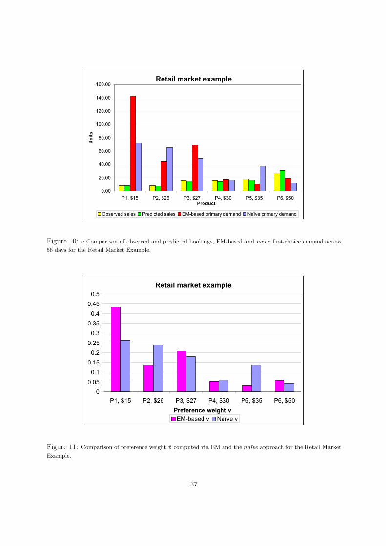
Retail market example

0.00

20.00

40.00

60.00

80.00

100.00

120.00

140.00

160.00

P1, $15 P2, $26 P3, $27 P4, $30 P5, $35 P6, $50Product

Un

its

Observed sales Predicted sales EM-based primary demand Naïve primary demand

Figure 10: e Comparison of observed and predicted bookings, EM-based and naıve first-choice demand across

56 days for the Retail Market Example.

Retail market example

0

0.05

0.1

0.15

0.2

0.25

0.3

0.35

0.4

0.45

0.5

P1, $15 P2, $26 P3, $27 P4, $30 P5, $35 P6, $50

Preference weight v

EM-based v Naïve v

Figure 11: Comparison of preference weight v computed via EM and the naıve approach for the Retail Market

Example.

37