Policy Research Working Paper 8878

Estimating Poverty in India without Expenditure Data

A Survey-to-Survey Imputation Approach

David NewhousePallavi Vyas

Poverty and Equity Global Practice June 2019

Pub

lic D

iscl

osur

e A

utho

rized

Pub

lic D

iscl

osur

e A

utho

rized

Pub

lic D

iscl

osur

e A

utho

rized

Pub

lic D

iscl

osur

e A

utho

rized

Produced by the Research Support Team

Abstract

The Policy Research Working Paper Series disseminates the findings of work in progress to encourage the exchange of ideas about development issues. An objective of the series is to get the findings out quickly, even if the presentations are less than fully polished. The papers carry the names of the authors and should be cited accordingly. The findings, interpretations, and conclusions expressed in this paper are entirely those of the authors. They do not necessarily represent the views of the International Bank for Reconstruction and Development/World Bank and its affiliated organizations, or those of the Executive Directors of the World Bank or the governments they represent.

Policy Research Working Paper 8878

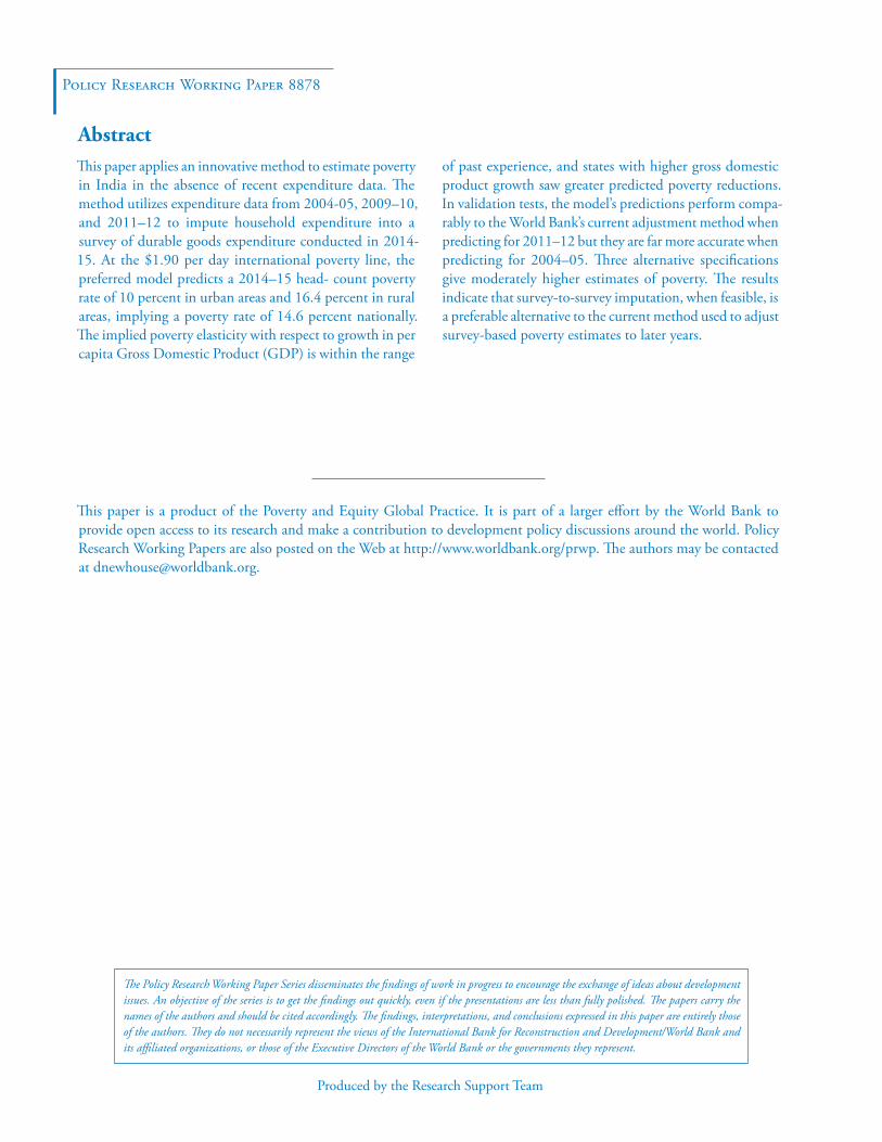
This paper applies an innovative method to estimate poverty in India in the absence of recent expenditure data. The method utilizes expenditure data from 2004-05, 2009–10, and 2011–12 to impute household expenditure into a survey of durable goods expenditure conducted in 2014-15. At the $1.90 per day international poverty line, thepreferred model predicts a 2014–15 head- count povertyrate of 10 percent in urban areas and 16.4 percent in ruralareas, implying a poverty rate of 14.6 percent nationally.The implied poverty elasticity with respect to growth in percapita Gross Domestic Product (GDP) is within the range

of past experience, and states with higher gross domestic product growth saw greater predicted poverty reductions. In validation tests, the model’s predictions perform compa-rably to the World Bank’s current adjustment method when predicting for 2011–12 but they are far more accurate when predicting for 2004–05. Three alternative specifications give moderately higher estimates of poverty. The results indicate that survey-to-survey imputation, when feasible, is a preferable alternative to the current method used to adjust survey-based poverty estimates to later years.

This paper is a product of the Poverty and Equity Global Practice. It is part of a larger effort by the World Bank to provide open access to its research and make a contribution to development policy discussions around the world. Policy Research Working Papers are also posted on the Web at http://www.worldbank.org/prwp. The authors may be contacted at dnewhouse@worldbank.org.

Estimating Poverty in India without Expenditure Data

A Survey-to-Survey Imputation Approach∗

David Newhouse† Pallavi Vyas ‡

∗The authors thank Joao Pedro Azevedo, Benu Bidani, Urmila Chatterjee, Paul Corral, Fran-cisco Ferreira, Haishan Fu, Dean Jolliffe, Christoph Lakner, Daniel Mahler, Rinku Murgai, MinhNguyen, Sutirtha Roy, Carolina Sanchez-Paramo, Benjamin Stewart, Roy Van der Weide, andNobuo Yoshida for invaluable suggestions, help, and support. This paper was previously pub-lished as a working paper entitled ”Nowcasting poverty in India for 2014-15”, which is availableat: http://documents.worldbank.org/curated/en/294251537365339600/Nowcasting-Poverty-in-India-for-2014-15-A-Survey-to-Survey-Imputation-Approach†World Bank Group, Washington DC, and IZA., Bonn.‡Ahmedabad University, Ahmedabad and World Bank Group, Washington DC.

1

I Introduction

This paper explains the methodology and results of a survey to survey imputation

exercise that was used to generate headcount poverty estimates for India. India was

selected as a pilot case because of its size and importance, as well as the lack of recent

data on household living standards. The latest survey-based estimates of poverty are

from 2011-12. The most recent nationally representative survey that could be used

to impute poverty into a later year is the NSSO expenditure on services and durables

survey of 2014-15. The resulting poverty estimates from the imputation informed

the 2015 poverty estimates, which are the most recent that are currently available,

marking the first time that the World Bank used this type of method as an input

into its global and regional poverty estimates.

Understanding trends in poverty in India is not only vital to Indian policy makers

to measure changes in the welfare of the poor, but also has major implications for

regional and global estimates of the prevalence of poverty. In 2013, an estimate of

the number of extreme poor in India, defined as those consuming less than $1.90 per

day per person, numbered 250 million 1. This means that India accounted for over

a quarter of the global total of 783 million extreme poor. Although Nigeria has now

likely passed India as the nation with the largest number of extremely poor persons,

accurately monitoring India’s progress in the fight against extreme poverty remains

critical to assess progress towards the goal of reducing poverty to less than 3% by

2030.

The second motivation for undertaking a modeling exercise is that the typical method

used by the World Bank to adjust poverty to a later year tends to overestimate the

pace of poverty decline. When estimating global and regional poverty rates, the

World Bank usually adjusts or “lines up” survey data from a variety of years to a

common year, by scaling up the measured levels of household per capita consumption

to account for growth in the intervening years. For example, to “line up” a survey

from 2012 to 2015, each household’s per capita consumption, measured in 2012,

would be assumed to grow at the same rate. In most countries, this common rate

of growth is assumed to be equal to the growth in household final consumption

expenditure (HFCE) during the intervening period.2 Because it is a component of

the national accounts, HFCE is published annually and can therefore be used to line

up the survey means to any later year.

1Estimate is based on the traditional line-up method explained below.2In some countries, growth in per capita GDP is used instead of final household consumption

expenditure.

2

Unfortunately, however, growth in HFCE tends to substantially exceed mean con-

sumption growth in household surveys.3 One study, for example, concludes that on

average only about half of the growth in HFCE was reflected in growth in survey

consumption.4 This is partly because official surveys face severe challenges obtain-

ing accurate measures of welfare for the very wealthy. Because there are few very

wealthy households, they may not be included in the sample. Wealthy households are

more likely than poor households to refuse to participate in the survey, and tend to

underreport their income or consumption. However, there are also good reasons why

national accounts data may overestimate growth in mean income or consumption,

including the use of outdated ‘rates and ratios’ based on old survey data.5

Because of the systematic discrepancy between growth in national accounts data

and household surveys, using HFCE to adjust survey data is prone to overstating

poverty reduction for countries that lack a recent survey such as India. In fact,

past analysis from India demonstrates how the typical line up adjustment procedure

can greatly overestimate poverty decline, using data from 2004-05 and 2009-10.6

Estimates were generated for 2009-10 by lining up the 2004-05 data to 2009-10,

applying the HFCE growth rate during that period. These line-up estimates for

2009-10 were then compared with measurements from actual survey data from that

year. The line-up procedure generated an estimated reduction in poverty from 41.6

to 13.4 percent, whereas the actual data from 2009-10 yielded a poverty rate of

32.7%.7 In other words, the line-up method overstated the decline in poverty by

19 percentage points. However, virtually all of the discrepancy between the line-

up estimate and the actual data resulted from consumption expenditure growth in

the national accounts exceeding mean welfare growth in the survey. In contrast,

assuming that the 2004-05 welfare distribution remained constant except for a scale

factor created negligible error. In this case, assuming that the distribution of welfare

changed by a common scale factor was fine; the real problem was determining what

factor should be used to scale up measured welfare in the initial year.

The concern that growth in the national accounts exceeds growth in survey mean

welfare motivates the use of a survey-to-survey imputation method to determine an

appropriate scale factor or “pass-through rate” to apply to HFCE. The major por-

tion of the exercise involves estimating poverty at the $1.90 line in 2014-15, using

3See Edward and Sumner (2013), Hillebrand (2008), Korinek, Mistiaen, and Ravallion (2006),Deaton and Kozel (2005), Ravallion (2003) and Minhas (1988).

4Ravallion (2003).5Deaton and Kozel (2005).6Jolliffe (2014) p.253.7These figures are based on the older, $1.25 poverty line (in 2005 PPP).

3

an econometric model estimated at the household level. Urban and rural sectors

are modeled separately, because they differ in fundamental ways.8 The model draws

on four rounds of past Indian National Sample Survey data, namely the 61st, 66th,

68th, and 72nd rounds, which were fielded in 2004-05, 2009-10, 2011-12, and 2014-15

respectively.9 The 2014-15 survey, unlike the three previous rounds used in this exer-

cise, did not collect information on aggregate household consumption and therefore

cannot generate direct estimates of poverty. The 2014-15 survey, however, contains

information on several household characteristics that are also present in past rounds

and are reasonably well-correlated with per capita consumption.10 These common

characteristics include household age, size, caste, religion, a few labor market vari-

ables, and expenditure on three categories of services that are asked in the same way

as previous rounds.

The analysis estimates a regression model that predicts household per capita con-

sumption using these common household characteristics, plus contemporaneous rain-

fall shocks and a linear time trend. Most coefficients are allowed to vary over time

in a linear way, slightly relaxing the usual strong assumption that the relationship

between the explanatory variables and log welfare remains constant over time.11 The

model is estimated using data from the first three rounds of the survey. The coeffi-

cients from this regression model were then applied to measured values of the same

common characteristics in the 2014-15 survey, as well as 2014-15 rainfall levels, to

repeatedly simulate levels of welfare and poverty. The results of these simulations

were aggregated to generate estimates of poverty headcount rates and their standard

errors.

This exercise is similar in spirit to the adjustments for non-comparability in the

consumption aggregate that led to “the great Indian poverty debate”.12 Since then,

this type of nowcasting exercise has also been carried out in several other countries.13

While this method has not yet been successfully applied to estimate changes in

inequality, a significant body of evidence now exists that out of sample predictions

8Also, India is one of three countries for which separate poverty estimates are presented bythe World Bank for urban and rural areas.

9Unfortunately, data between 1993 and 2004-05 were unavailable because the welfare aggre-gate in the 1999-2000 round was not comparable.

10In the pooled regression including 2004-05, 2009-10, and 2011-12 data, the R2s are 0.57 forurban areas and 0.46 for rural areas (Table 14 (Appendix).)

11Nguyen and van der Weide (2018).12Deaton and Dreze (2002) and Kijima and Lanjouw (2003) Deaton and Kozel (2005).13See, for example, Christiaensen and Stifel (2007) in Kenya, Newhouse, Shivakumaran, Taka-

matsu, and Yoshida (2014) in Sri Lanka, Douidich, Ezzrari, Van der Weide, and Verme (2016) inMorocco, and Dang, Lanjouw, and Serajuddin (2017) in Jordan.

4

from models estimated on past data generate credible estimates, in a variety of

country contexts, of poverty headcount and gaps.

The preferred model generates an estimate of 10.0% in urban areas and 16.8% in

rural areas, which implies an overall poverty level of 14.6% for 2014-15 (Table 1 and

Figure 1). The estimate is consistent with poverty reduction from 2004-05 to 2011-

12 in rural areas and suggests a slight deceleration in poverty reduction in urban

areas (Table 2). This in turn implies that the elasticity of poverty with respect to

growth of per capita GDP was -2.11, which is within the range of past experience.

Reassuringly, when looking at the state level, predicted poverty reduction is greater

in states with higher rates of GDP growth.

We use two main tests to validate the survey-to-survey imputation models. The first

estimates a model with the same specification, using data from 2004-05 and 2009-10,

to predict into 2011-12. These predictions are then compared with actual measured

levels of poverty from the national sample survey. In a similar, vein, the second

validation test uses data from 2009-10 and 2011-12 to predict backwards to 2004-05.

This is a much more challenging exercise because the data from two years apart are

being used to extrapolate five years in the past.

While the traditional line-up method performs slightly better than our preferred

specification in 2011-12, it gives wildly implausible estimates when projecting back

to 2004-05. To be specific, the standard line-up method is off by only a percentage

point in 2011-12 but exaggerates poverty by 25 percentage points when predicting

back to 2004-05. Our preferred model performs much better on average, as the

discrepancy is about 2 percentage points in 2011-12 and about 3 percentage points

in 2004-05.

The traditional line-up method happens to do well when projecting forward into

2011-12 because growth in mean reported consumption in the survey was unusually

high between 2009-10 and 2011-12 and nearly matched growth in HFCE. This is a

sharp break from the pattern observed during the previous period, and in most other

contexts. It remains to be seen whether this correspondence between HFCE and

survey mean growth will be sustained, but there are at least two reasons to speculate

it may not be. The first is that survey-based consumption may be more responsive

than national account data to weather shocks. India experienced significant droughts

during 2004 and 2009, followed by above-average rainfall in the 2011 season. To the

extent that survey-based consumption is more sensitive than national accounts to

agricultural income, favorable rainfall in 2011 would cause a larger jump in survey

5

consumption than HFCE.14The second factor is the recovery from the 2008 financial

crisis, which is distinctly visible in the 2009 national accounts data. Survey-based

consumption, however, may have taken longer to recover. Both factors could have

contributed to the unusually large increase in mean consumption observed between

2009-10 and 2011-12, which counteracted the usual tendency for HFCE growth to

exceed growth in mean consumption. We know of no reason to believe, however, that

growth in HFCE will accurately reflect growth in mean consumption going forward.

Turning back to the model predictions, we consider three alternative specifications

that impose more restrictive assumptions. These estimate a slower poverty decline,

with estimated headcount rates ranging from 17.4 to 19.1 percent. In contrast, the

traditional line-up method shows a much more rapid decline in poverty, from 21.6%

in 2011-12 to 10.9% in 2014-15. This shows that the choice of modeling assumptions

matters, at least in this case.

The final step is to use the estimates for 2014-15 from the econometric model to

generate the poverty estimate for India for 2015 used in the global estimates. This

was done by estimating an appropriate fraction, or “pass-through rate”, to apply to

growth in HFCE, thereby assuming that only a portion of the HFCE growth is passed

through to growth in mean welfare in the household survey. Pass-through rates were

selected to match the $1.90 headcount poverty estimates from the survey-to-survey

imputation model for 2014-15, which were 10% in urban areas and 16.8% in rural

areas. These were then used to calculate estimates for 2015, based on the scaled

down growth rate of HFCE.15

The rest of this paper is organized as follows. The next section reviews the data used

for the analysis. Section III turns to the methodology. It discusses the estimation

method and the process used to select the set of predictor variables, and examines

the results of four alternative specifications to the model. Section IV compares the

preferred model’s predictions for 2014-15 to the usual method used to project poverty

forward, and investigates which specific variables are accounting for the change in

average welfare predicted by the model. Section V shows that the estimated poverty

rate implies a reasonable elasticity of poverty reduction with respect to growth,

verifies that implied poverty reduction is greater in fast-growing states, and examines

the model’s predictions at higher poverty lines. Section VI briefly describes how the

2014-15 estimates were used to generate poverty estimates for 2015, and Section VII

concludes.14According to the Economic Survey 2017-18 of the Ministry of Finance in India, agriculture

employs over half of Indian workers but only contributes 17 to 18 percent of India’s GDP.15The 2015 estimates can be viewed at http://iresearch.worldbank.org/PovcalNet/povDuplicateWB.aspx.

See http://iresearch.worldbank.org/PovcalNet/WhatIsNew.aspx for further details.

6

II Data

In order to obtain estimates of welfare for 2014-15, we first identify variables that

are common both to the three earlier consumption surveys and the 2014-15 round.

The surveys have five demographic variables in common. They are household size,

age of household members, gender, religion, and caste contained in the “household

characteristics” section of each survey. The three common labor market variables

are the household’s principal industry, principal occupation and principal means of

livelihood.

The principal industry of a household is determined according to the National Indus-

trial Classification (NIC) 2008 code for the NSSO72, NSSO68 and NSSO66 surveys

and the NIC 1998 code for the NSSO61 survey.16 Regarding the principal occupa-

tion, the NSSO72, NSSO68 and NSSO66 surveys categorize households according to

the National Classification of Occupations (NCO) 2004 code and the NSS061 survey

according to the NCO 1968 code. To ensure consistency, the occupation categories

are harmonized across survey years. We further group households into high skill,

middle skill and low skill occupation categories.17 The household’s principal means

of livelihood is determined from the “household type” variable. The categories are

self-employed, regular wage/salary earning, casual labor and “other”.18

In addition, the surveys ask questions regarding expenses on miscellaneous services

such as household service (domestic help, barber, beauty, laundry, priest, grinding,

tailor), recreation (cinema/theater, fairs/picnics, club fees, photography, VCD/DVD

on hire) and transport (conveyance related expenses). We also include a district-level

rainfall variable that accounts for deviations from the mean.19

Second, we ensure that the wording and recall periods on the questions are com-

parable over time. Both different wording and/or recall periods would change the

16Households whose principal industry is agriculture, forestry or fishing are classified into theagricultural sector. Those that work principally in mining, manufacturing, construction or for theutilities are industrial sector households. Lastly, service sector households are those that work inwholesale or retail trade, food and accomodation, transportation and storage, information andcommunication, finance and insurance, real estate, professional and scientific, administrative andsupport, public administration and defense, education, health or arts and recreation.

17Legislators, senior officials, managers, professionals, technicians and associate professionalsare in the high skill category. Clerks, service workers, shop and market sales workers are classifiedas middle skill. Workers in agriculture and fishery, craft and related trades, plant and machineoperators, assemblers and those in “elementary” occupations are classified as low skill.

18For rural areas, each of the categories are reported as agriculture and non-agriculture sub-classifications that we group together to make them comparable to the urban areas.

19The rainfall data were taken from the Climate Hazards Group InfraRed Precipitation withStation (CHIRPS) data set on precipitation (Funk, Verdin, Michaelsen, Peterson, Pedreros, andHusak (2015)).

7

interpretation of the relevant variables and thus affect the predictability of our model.

We find for all the variables that we include, the questions are similar across surveys.

On the other hand, there are questions related to expenditure on consumer durables

in both surveys that we do not include. First, there are discrepancies in relation

to the wording of the questions between the NSSO72 and earlier surveys.20 Second,

the recording of possession and expenditures was different between the surveys. We

observed the discrepancies in the manuals provided to the surveyors.21

Third, we confirm that the sampling frame is similar across all surveys. Like the

earlier rounds, the NSSO72 is a multi-stage stratified survey of all states/union ter-

ritories in India. To more accurately represent population density, for the 72nd round

the primary sampling units (PSUs) are selected from the 2011 census list of villages

in the rural sector while for the earlier rounds they are drawn from the 2001 census

list of villages. Also, the number of PSUs are slightly higher, 14,088, in the 72nd

round. For each of the earlier surveys, 12,784 PSUs are selected.22 For the urban

sector, in all surveys the PSUs are sampled from the Urban Frame Survey (UFS)

blocks. For all surveys, the methodology to select the PSUs, the strata, sub-strata

and the ultimate stage units (USUs) or households remains the same.23

20The NSSO61, NSSO66 and NSSO68 ask about “expenditure for purchase and construction(including repair and maintenance) of durable goods for domestic use” and the NSSO72 asksabout “expenditure on durable goods acquired during the last 365 days other than those usedexclusively for entrepreneurial activity”. Second, the NSSO61, NSSO66 and NSSO68 (type 1 sur-vey) has questions for a 30 day and a 365 day recall period while the question on the NSSO72only asks about expenditure for the 365 recall period. Third, the NSSO61, NSSO66 and NSSO68asks about expenditure for “purchase and construction”, while the NSSO72 asks about “acqui-sition” rather than explicitly about purchase. Fourth, the NSSO61, NSSO66 and NSSO68 askabout purchase for “domestic use” while the NSSO72 asks about goods “other than those usedexclusively for entrepreneurial activity”. This includes the total value of raw materials, servicesand/or labor charges and any other charges. There is no explicit mention of “construction” or“repair and maintenance” in the NSSO72, but there is a value of components column that mostlikely includes raw materials used in construction. Fifth, in the NSSO68, there is a separate ques-tion on whether the good was bought for “hire purchase”. The surveyor is asked to make the dis-tinction between “hire purchase” and a loan. The NSSO72 instruction manual does not mentionanything about goods bought on “hire purchase”.

21First, if an asset was bought and sold during the reference period, it is recorded in the ear-lier NSSO surveys but not in NSSO72. Second, in the earlier surveys if the item has been pur-chased but not yet in the household’s possession, the expenditure is recorded by the surveyor.However, in the NSSO72 a durable good that is not in the household’s possession even if full pay-ment has been made is not included. Third, if the durable good is in possession but has not beenpaid for, it is not included in the earlier NSSO surveys but is included in the NSSO72 (Instruc-tions to Field Staff, Chapter Four).

22The NSSO refers to PSUs as First Stage Units (FSUs). The term ’village’ is Panchayatwards for Kerala.

23In the event that the population is greater than 1,200 in a PSU, the PSU is divided into“hamlet groups” “sub-blocks” in the rural and urban PSUs, respectively.

8

A Descriptive Statistics

Tables 3 and 4 report the mean values of the variables used in the model by year,

for urban and rural areas. The descriptive statistics generally reflect India’s rapid

economic development. Average log per capita consumption, in real terms increased

from 4.5 to 4.74 between 2004-05 and 2011-12. When expressed in levels, per capita

consumption grew approximately 24% growth over the seven-year period, or 3.1% a

year. Household size steadily fell during this time. In the decade between the first

and last survey, the share of the population living in households with 4 or fewer

persons rose from 39 to 47 percent in urban areas, and from 29 to 35 percent in

rural areas. A byproduct of smaller households is a drop in the share of household

members that are children ages 0-14, which fell by 5 percentage points in both urban

and rural areas. Regular wage work became slightly more prevalent in urban areas,

and the share of rural workers working in agriculture declined 3 percentage points,

as industrial work became more common in rural areas.

Average spending on transport declined in 2014-15 after a consistent rise between

2004-05 and 2011-12. In contrast, expenditure on household miscellaneous services

and recreational spending showed a continual strong increase from 2004-05 to 2014-

15. The drop in transport expenditures may in part result from differences in the

components of transport expenditure in 2014-15.24 To the extent this is causing the

drop in reported transport expenditure, the model may underestimate poverty re-

duction. We therefore also consider a model that only includes whether households

reported any consumption on these three items in the past month, rather than in-

cluding the amounts, as a robustness check to see how much including expenditure

amounts matters.

The final rows of Tables 3 and 4 report the population-weighted mean rainfall, across

districts, in terms of deviation from historical district means. Monsoons in India typ-

ically occur between June and October, making the third quarter rainfall important

for agricultural production. Table 4 indicates that in rural areas, rainfall was be-

low average in the second half of 2004, the third quarter of 2009 and the first two

24While the recall periods are the same and most of the categories of transportation expendi-ture are similar across surveys, in the NSSO72 the surveyors were asked to exclude expenditureon fuel for one’s own transport. The consumption expenditure surveys do include expenditureon petrol and diesel for vehicles. Also, in the NSSO72 survey questions regarding transportationexpenditure were asked separately for overnight and non-overnight journeys. We include the ex-penses for both types of journeys as well as expenditure on services incidental to transport tomake it comparable to the consumption expenditures surveys where the questions do not makeany distinction on the type of journey and also include expenditures on services incidental totransport.

9

quarters of 2010. On the other hand, rainfall was substantially above average in

the third quarter of 2011, and close to exactly average in the third quarter of 2014.

As mentioned above, favorable rainfall may have contributed to the strong growth

in survey consumption between 2009-10 and 2011-12, but did not continue in the

summer of 2014.

III Empirical Methodology

A Econometric Model

The specification of the model is based on the small area estimation (SAE) methodol-

ogy originally proposed by Elbers, Lanjouw, and Lanjouw (2003). This methodology

generates a joint distribution of economic welfare and independent variables in the

target data set, where a welfare measure is not available. The process consists of two

steps. The first involves estimating the relationship between economic welfare and

explanatory variables in the source data set, in which a welfare measure is available.

The parameters are then used to simulate economic welfare into the target data set.

The first step in this analysis is to estimate the relationship between household

per capita consumption expenditure (the measure of economic welfare) and other

explanatory variables, in the three available source data sets with consumption data.

The explanatory variables are those that are available in both the source and target

data sets. The regression is a log linear specification relating per capita consumption

expenditure to household and regional variables using the 2004-05, 2009-10 and 2011-

12 surveys (equation 1).25 The welfare measure is ycht, which is household per capita

expenditure for a household in cluster c and household h, interviewed in survey round

t. A cluster is a primary sampling unit (PSU) as defined in the NSSO surveys. For

all surveys, ycht is measured in 2011 rupees using separate CPI indices for urban and

rural areas.26

The Xh vector in equation (1) consists of an intercept plus household level demo-

graphic variables, labor market variables and expenses on miscellaneous services.

Expenses on miscellaneous services for all survey years are measured in 2011 ru-

pees.27 The vector Zh is a subset of the Xh variables whose coefficients are allowed

to vary linearly over time. In order to avoid introducing severe multicollinearity into

25NSSO61, NSSO66 AND NSSO68. The coefficients in this semi-log model are interpreted as arelative change in welfare as a result of an absolute change in the explanatory variables.

26For rural areas, we use the CPI for Agricultural and Rural Laborers and for urban areas theCPI for Industrial workers. Source: CEIC (from Labor Bureau Government of India).

27The CPI indices are the same as those used for the welfare measure, ycht.

10

the model, only a subset of the Xh variables are interacted with a linear time trend

(Nguyen and van der Weide (2018)). The Xd vector consists of district level variables

calculated as means of household variables for each district. This vector also includes

a measure of rainfall shocks, which is the district’s deviation from mean historical

rainfall. District level characteristics are included both to improve the accuracy of

model predictions, and to generate more accurate estimates.28 Area means are calcu-

lated at the district rather than the PSU level due to measurement error arising from

insufficient numbers of observations per PSU. As with household characteristics, a

subset of district characteristics are interacted with time trends (Zdt).

ln(ycht) = Xhchtγ1 + Zh

chttγ2 +Xdctγ3 + Zd

cttγ4 + γ5t+ ucht (1)

The regressions are weighted using population weights.29 In addition, because of im-

portant differences in consumption patterns in urban versus rural areas, and because

poverty rates are reported separately for urban and rural India, separate models are

estimated for each sector.

Taking X as the vector of all variables and β as the vector of coefficients, equation

(1) can be rewritten as:

ln(ycht) = X ′β + ucht (2)

An initial estimate of β is obtained using weighted Ordinary Least Squares (OLS)

(equation 2). The consumption spending of households within a cluster are assumed

to be correlated. To allow for this within-cluster correlation, the random disturbance

term uch has a cluster, ηc, and a household component εch. Therefore, the random

disturbance term can be written as,

uch = ηc + εch (3)

The variables ηc and εch are assumed to be independent of each other and uncorre-

lated with the explanatory variables. We do not allow for heteroskedasticity in the

cluster component of uch, due to the small number of clusters.30 However, the house-

hold error term, εch, is assumed to be heteroskedastic reflecting unequal variances in

the error terms across households.

Because of heteroskedasticity in the error term and spatial correlation from the in-

troduction of ηc, we re-estimate equation (2) using Generalized Least Squares (GLS).

28Elbers, Lanjouw, and Leite (2008).29Household weights are multiplied by household size to calculate population weights.30Elbers, Lanjouw, and Lanjouw (2003).

11

The weights for the GLS specification are the predicted variances of the error terms

from the OLS regression. We estimate the variance of the error term parametrically

as specified in Elbers, Lanjouw, and Lanjouw (2003) and Nguyen, Corral, Azevedo,

and Zhao (2017). The variance model has a logistic form with (ε2ch) as the depen-

dent variable (equation 4). In equation 5, the dependent variable is the estimated

variance, derived from the residuals of the first OLS regression. The explanatory

variables of the variance model are chosen using the Least Absolute Shrinkage and

Selection Operator (LASSO) method (Tibshirani (1996)).31 The estimates from the

LASSO regression and the residuals are then used to predict the variance of (εch)

(equation 6).

E[ε2ch] = σ2εch =

[AeZ

′α +B

1 + eZ′α

](4)

ln

[ε2ch

A− ε2ch

]= Z ′

chα + rch (5)

σ2εch≈[AeZ

′α

1 + eZ′α

]+

1

2V ar(r)

[AeZ

′α(1− eZ′α)

(1 + eZ′α)3

](6)

The predicted variances are used to re-estimate equation (2) using GLS (equation

(7)).

ln(ycht) = X ′βGLS + ucht (7)

Next, we estimate predicted welfare using estimates from the analysis in the first

step. Since we would like to generate a joint distribution of welfare, and not solely

the expected value, we use Monte-Carlo simulations to generate 100 simulated dis-

tributions of welfare. In equation (8), β, ηc and εch are vectors from the simulations.

ycht = X ′β + ηct + εcht (8)

Following the literature on small area estimation, we make the following assumptions

for the simulations. The vector β is drawn from a normal distribution with mean

βGLS and variance Var(βGLS).

β ∼ N(βGLS, V ar(βGLS))

31In this method all district and household characteristics used in step 1 are included on theright- hand side. The resulting estimates include zero coefficients for several variables, therebyselecting the remaining variables with non-zero coefficients for the variance model.

12

The cluster component of the error term, ηc, is drawn from a normal distribution

with mean 0 and variance, σ2η. The data generating process of the variance term is

assumed to follow a gamma distribution.

ηc ∼ N(0, σ2η)

σ2η ∼ Gamma(σ2

η, V ar(σ2η))

The household component of the error term, εch, is drawn from a normal distribution

with mean 0 and the variance predicted by equation (6). The variance term is

calculated by applying the parameters from the source data (equation 5) to the

2014-15 data (equation 6).

εch ∼ N(0, σ2εch

)

The 100 simulated values, β, α, ηc and εch are used to obtain a vector of 100 simulated

welfare estimates, ych. The mean of the 100 simulations gives the point estimate of

household expenditure. The standard error of the poverty estimate is calculated using

Rubin’s rules (Rubin (2004)) which takes into account the variation both within

and across simulations. We use the STATA package SAE developed by (Nguyen,

Corral, Azevedo, and Zhao (2017)) to carry out the estimation and the Monte Carlo

simulations.

B Variable Selection

The process described above requires a set of right-hand side variables to estimate

equation (1). We elected for a model selection process that emphasizes transparency

and simplicity, while addressing concerns that excessive multi-collinearity could jeop-

ardize the model’s out-of-sample predictive accuracy. Multicollinearity, which occurs

when one or more right-hand side variables are highly correlated with the remaining

right-hand side variables, leads to imprecise coefficient estimates. Coefficient esti-

mates that are imprecise, especially for important drivers of predicted welfare change

such as the coefficient on the linear time trend, will reduce the accuracy of the pre-

dictions. In addition, models with greater multicollinearity among the regressors

are fragile to minor changes in the model’s specification such as removing particular

variables.

We start with the set of candidate variables listed in Tables 3 and 4, which are

common to both surveys. For each variable, we also take district means, in order to

improve the accuracy of the prediction and their standard errors. Finally, a subset

13

of household and district mean variables are interacted with the year of the survey,

allowing the coefficients to vary linearly over time. This reflects the fact that the

association between certain characteristics and welfare changes over time. We restrict

the model to interactions with a linear time trend because of the importance of

maintaining a consistent model for both the estimation and the validation exercise.

For the validation exercise, only two rounds of data are available to estimate the

model, leaving insufficient degrees of freedom to estimate polynomial time trend

interactions.

To alleviate concerns about multicollinearity, we sequentially calculate variance in-

flation factors (VIF) for all variables. The VIF for a coefficient is equal to the

reciprocal of one minus the R2 from regressing that variable on the full set of other

right-hand side variables. Therefore, the greater the variation in a variable that can

be explained by the other independent variables, the greater the VIF. We follow the

informal rule of thumb most prevalent in past studies, which recommends concern

about the model if any VIFs exceed 10.32 We therefore sequentially remove the vari-

able with the largest VIF if that variable exceeds 10, with the exception of the time

trend variable. This variable was deemed critical to the model because it accounts

for most of the change in predicted mean consumption per capita between 2011-12

and 2014-15. This process was carried out separately for urban and rural areas, and

eliminated 23 variables in urban areas and 21 in rural areas. Selecting the optimal

set of variables for prediction is an active area of research and no clear consensus has

emerged regarding the most appropriate method to use. The procedure described

above successfully reduces multi-collinearity while remaining simple to apply and

explain.

C Model Selection

Besides the primary model that was ultimately used for the estimation, we consider

three alternative specifications. In one we interact each district level variable with

a linear time trend. We refer to this model as the “District dummies*Time Trend”

model. The district dummies subsume the district mean characteristics, which are

dropped from this specification. The inclusion of district time trends in the model

has the advantage of accounting for unobserved characteristics of the district whose

effects vary over time in a linear way. The potential downside of the district time

32See Kennedy (1992), Chatterjee and Hadi (2012), Menard (1995), and others quoted inO’Brien (2007). As noted by O’Brien, removing variables changes the interpretation of the co-efficients; however, since the objective of this model is prediction, this is less of a concern than ifthe focus were on the regression coefficients.

14

trends model is that it extrapolates past trends to predict district mean welfare in

2014-15 rather than using actual data on district characteristics in 2014-15. While

this is more likely to give a rate of poverty reduction in line with past trends, it will

ignore the signal from district level indicators in characteristics.

The second alternative model tested includes dummy variables for the three types

of expenditure instead of the actual expenditure amounts. The dummy variables

are equal to one if the household incurred any expenditure for the particular item.

We refer to this model as “Expenditures at the Extensive Margin”. This has the

advantage of potentially being more robust to outliers in consumption, as well as

changes in the way that the question was asked. However, it potentially ignores

valuable information on the level of expenditures.

Lastly, we use only the 2011-12 data to predict into 2014-15. Because only one round

of data is used to estimate the model, no variables are interacted with a time trend.

We refer to this as the “Constant Coefficient” model, which has been utilized in past

studies of survey to survey imputation.

We report predicted poverty rates of the four models in Table 5. We choose the

primary model as our preferred specification because it utilizes all the available data,

including levels of expenditure, imposes the least restrictive modeling assumptions on

the data and has the most accurate predictions. We validate each model’s predictive

quality by conducting two tests. First, for each specification we use data from 2004-

05 and 2009-10 to predict poverty in 2011-12. We refer to this as forward projection.

In the second analysis, we reverse project poverty in 2004-05 using the 2009-10

and 2011-12 data (see e.g., Deaton and Dreze (2002)). In the forward and reverse

projections, we compare the actual versus predicted headcount of poverty, in 2011-

12 and 2004-5 respectively.33 Our final choice of model is based on which yields the

most accurate estimates of poverty, on average, in both tests.

C.1 Forward projection into 2011-12

Table 6 compares actual poverty in 2011-12 with the predictions of the four models.

For urban areas, the projection of model 1 (14.6%) is closest to the actual poverty

number (13.4%). Model 3, the extensive margin model, gives predictions that are

closet to the actual poverty number for rural areas (24.8%), followed by model 1

(27.4%). Therefore, models 1 or 3 could be possibilities for the final choice based on

the forward projection test.

33Using the $1.90 per day threshold.

15

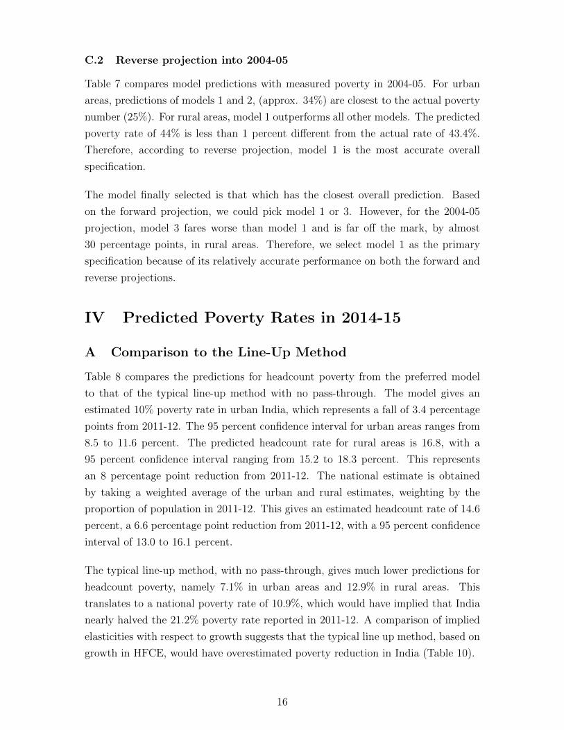
C.2 Reverse projection into 2004-05

Table 7 compares model predictions with measured poverty in 2004-05. For urban

areas, predictions of models 1 and 2, (approx. 34%) are closest to the actual poverty

number (25%). For rural areas, model 1 outperforms all other models. The predicted

poverty rate of 44% is less than 1 percent different from the actual rate of 43.4%.

Therefore, according to reverse projection, model 1 is the most accurate overall

specification.

The model finally selected is that which has the closest overall prediction. Based

on the forward projection, we could pick model 1 or 3. However, for the 2004-05

projection, model 3 fares worse than model 1 and is far off the mark, by almost

30 percentage points, in rural areas. Therefore, we select model 1 as the primary

specification because of its relatively accurate performance on both the forward and

reverse projections.

IV Predicted Poverty Rates in 2014-15

A Comparison to the Line-Up Method

Table 8 compares the predictions for headcount poverty from the preferred model

to that of the typical line-up method with no pass-through. The model gives an

estimated 10% poverty rate in urban India, which represents a fall of 3.4 percentage

points from 2011-12. The 95 percent confidence interval for urban areas ranges from

8.5 to 11.6 percent. The predicted headcount rate for rural areas is 16.8, with a

95 percent confidence interval ranging from 15.2 to 18.3 percent. This represents

an 8 percentage point reduction from 2011-12. The national estimate is obtained

by taking a weighted average of the urban and rural estimates, weighting by the

proportion of population in 2011-12. This gives an estimated headcount rate of 14.6

percent, a 6.6 percentage point reduction from 2011-12, with a 95 percent confidence

interval of 13.0 to 16.1 percent.

The typical line-up method, with no pass-through, gives much lower predictions for

headcount poverty, namely 7.1% in urban areas and 12.9% in rural areas. This

translates to a national poverty rate of 10.9%, which would have implied that India

nearly halved the 21.2% poverty rate reported in 2011-12. A comparison of implied

elasticities with respect to growth suggests that the typical line up method, based on

growth in HFCE, would have overestimated poverty reduction in India (Table 10).

16

B Which Variables Account for Growth in Mean Welfare?

Which variables in the model account for the bulk of the change in poverty? While

this question is difficult to answer directly, indirect evidence is available by decom-

posing the growth in log per capita consumption predicted by the model. A natural

framework for better understanding the contribution of individual variables is the

classic Oaxaca-Blinder decomposition (Oaxaca (1973), Blinder (1973)). This tech-

nique decomposes the mean difference across two groups into a portion explained

by differences in endowments and a portion due to differences in returns. In this

case, the two groups are the households in the 2011-12 survey and the households

in the 2014-15 survey. We decompose the difference between the model’s mean pre-

dicted per capita consumption in 2014-15 and 2011-12. Because the means from

each year are generated by predictions from the same model, none of the difference

is attributable to changes in the coefficients (returns), and all of the change is due

to the mean of the predictor variables (endowments). These changes can easily be

decomposed into the portion due to each individual predictor variable, which helps

to identify the variables that account for the largest changes in the model.

Table 9 displays the results. Each cell represents the percentage of the total change

in mean log per capita consumption attributable to each variable. The time trend

alone, for example, explains 83 percent of the increase in urban areas and 80 percent

in rural areas. Notably, transport expenditure declined in real terms during this

period. This slowed the predicted increase in per capita consumption, particularly

in urban areas. The rainfall variables contributed to a relatively large share of the

increase in urban areas. However, the total increase in welfare was much smaller in

urban areas, meaning that in absolute terms rainfall’s contribution was similar in

urban and rural areas. As might be expected, changes in the means of livelihood

categories contribute a significant amount in urban areas, but much less in rural

areas. The results overall indicate that the time trend is a key driver of predicted

change in the model. However, transport expenditure plays a significant role, as

does the increase in service expenditure in rural areas. Finally, rainfall contributes a

significant amount in urban areas, as do changes in the types of jobs held by workers.

V Robustness Checks

We conduct three checks to assess the robustness of our model. First, we calculate

elasticities and semi-elasticities to see what the models’ predictions imply about the

change in extreme poverty with respect to real GDP growth. Second, we examine

17

predicted headcount rates at the state level to test whether the model generates

plausible predictions. Lastly, we examine estimated poverty rates at higher poverty

lines to ensure that they are reasonable. Ultimately, only the estimated urban and

rural poverty rates at the $1.90 line were used to determine the official poverty

estimates, by calculating an appropriate pass-through rate to apply to consumption

growth in the national accounts.

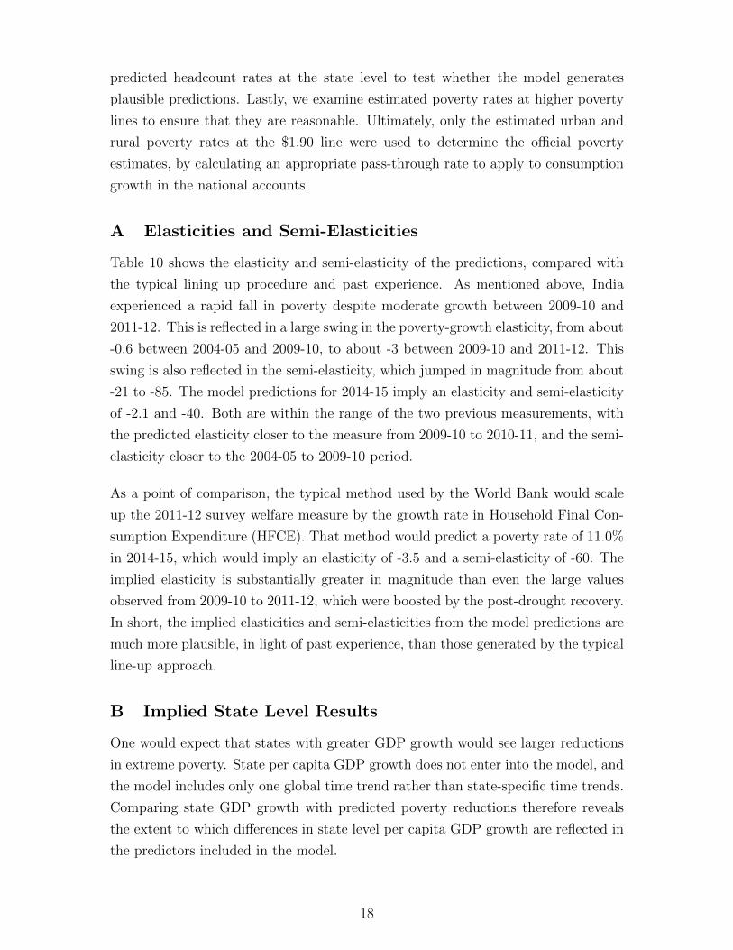
A Elasticities and Semi-Elasticities

Table 10 shows the elasticity and semi-elasticity of the predictions, compared with

the typical lining up procedure and past experience. As mentioned above, India

experienced a rapid fall in poverty despite moderate growth between 2009-10 and

2011-12. This is reflected in a large swing in the poverty-growth elasticity, from about

-0.6 between 2004-05 and 2009-10, to about -3 between 2009-10 and 2011-12. This

swing is also reflected in the semi-elasticity, which jumped in magnitude from about

-21 to -85. The model predictions for 2014-15 imply an elasticity and semi-elasticity

of -2.1 and -40. Both are within the range of the two previous measurements, with

the predicted elasticity closer to the measure from 2009-10 to 2010-11, and the semi-

elasticity closer to the 2004-05 to 2009-10 period.

As a point of comparison, the typical method used by the World Bank would scale

up the 2011-12 survey welfare measure by the growth rate in Household Final Con-

sumption Expenditure (HFCE). That method would predict a poverty rate of 11.0%

in 2014-15, which would imply an elasticity of -3.5 and a semi-elasticity of -60. The

implied elasticity is substantially greater in magnitude than even the large values

observed from 2009-10 to 2011-12, which were boosted by the post-drought recovery.

In short, the implied elasticities and semi-elasticities from the model predictions are

much more plausible, in light of past experience, than those generated by the typical

line-up approach.

B Implied State Level Results

One would expect that states with greater GDP growth would see larger reductions

in extreme poverty. State per capita GDP growth does not enter into the model, and

the model includes only one global time trend rather than state-specific time trends.

Comparing state GDP growth with predicted poverty reductions therefore reveals

the extent to which differences in state level per capita GDP growth are reflected in

the predictors included in the model.

18

Figure 2 displays, for each state, change in headcount poverty between 2011-12 and

2014-15, as predicted by the model, on the y axis. The x axis represents the real

annual state GDP growth during that period. Goa, which suffered a sharp decline

during this period, is a clear outlier. Whether Goa is included or excluded, there

is a clear negative correlation between state GDP growth and poverty reduction, as

would be expected. Figure 3 shows a comparable plot for the period from 2004-05

to 2011-2. With all states included, the relationship between state GDP growth and

poverty reduction between 2011-12 and 2014-15 is remarkably similar to the actual

relationship between state GDP growth and poverty reduction between 2004-05 and

2011-12. In particular, both show that a growth rate of 5% per year is associated

with about a one percentage point per year reduction in poverty, while a growth

rate of 10% is associated with a reduction of about two percentage points per year.

Excluding Goa from the more recent period makes the relationship between state

GDP growth and poverty reduction somewhat stronger, underscoring the point that,

as would be expected, the model predicts more rapid reductions in faster-growing

states.

C Higher Poverty Lines

Tables 11 and 12 and Figures 4 and 5 report the predicted poverty rates at the lower

middle- income line of $3.20 per day per person, and the upper middle- income line of

$5.50 per day per person. The predicted 2014-15 poverty rates for the $3.20 line are

60.3% in rural areas, 39% in urban areas, and 53.4% nationally. This is a moderate

reduction from the 2011-12 estimate of nearly 7 percentage point, or 12% at the

$3.20 line. The predicted poverty rates at the $5.50 line suggest a more modest

decline, from 89.7% in 2011-12 to a predicted rate of 85.6% in 2014-15 (Table 12).

This reflects the skewed nature of the welfare distribution, with larger numbers of

people near the $3.20 line being pushed out of poverty as the economy improves.

Finally, the predicted distribution can also be used to obtain an estimate of “shared

prosperity”, defined as the growth rate of mean consumption of the bottom 40%.

When averaging across the 100 simulations, the growth rate of consumption of the

bottom 40% amounts to 5.1% per year between 2009-10 and 2014-15, which is well

within the range exhibited by other countries(World Bank Group (2018)). Overall,

these predicted values for higher poverty lines appear to be consistent with past

trends.

19

VI Estimating the Pass-Through Factor to Gen-

erate Estimates for 2015

The previous sections describe in detail the methodology used to generate urban and

rural estimates of extreme poverty for 2014-15, as well as a battery of validation

and robustness checks designed to build confidence in the method and results. This

section considers the final portion of the exercise, which is the process of determin-

ing the appropriate pass-through factors to apply to Household Final Consumption

Growth that replicate these poverty rates. This portion has two main steps. The

first is to calculate a growth rate, that when applied uniformly to the 2011-12 welfare

distribution, generates the predicted 2014-15 poverty rate of 10.0% for urban areas

and 16.8% for rural areas. The appropriate growth rates are 9.6% in urban areas

and 12.6% in rural areas. The second step is to calculate these growth rates as a

fraction of HFCE growth during that period, which was 17.2%. Dividing 9.6 by 17.2

gives an estimated pass-through rate of 55.9% for urban areas. Similarly, dividing

12.6 by 17.2 gives the 73.3% pass-through rate for rural areas. These pass-through

rates were then applied to the 2011-12 distribution in order to project out to 2015.

The final $1.90 poverty rate for 2015 is 9.5% in urban areas, 15.3% in rural areas,

and 13.4% nationally.34

VII Conclusion

This analysis was motivated by concerns that the standard method of applying

growth in HFCE to the most recent survey measurement of per capita consump-

tion would overstate poverty reduction in India, and therefore the world. These

concerns were heightened by the age of the most recent available poverty data from

India, which was collected three and a half years before the 2015 target estimate.

This paper describes an alternative method for estimating poverty, which utilized

a more recent nationally representative survey from 2014-15 containing some of the

same demographic and socioeconomic characteristics collected in previous expendi-

ture surveys. These previous surveys were used to estimate a model, which was

then used to predict expenditure and poverty into the 2014-15 survey. This type

of statistical method has generated plausible headcount poverty estimates in other

countries and appears to work well in India as well, based on two validation exercises

and a variety of robustness checks. The model’s predictions imply an elasticity with

respect to growth that is in line with past experience, in contrast to the traditional

34Information on other lines can be obtained on the Povcalnet website.

20

line-up method, which gives elasticities that are significantly higher in magnitude

than previously observed. The model estimates plausible poverty rates at higher

poverty lines, and predicts greater poverty reduction in faster growing states. The

validation exercises show that in 2011-12, the imputation model fared slightly worse

than the typical method of applying HFCE growth to older survey data. When

predicting back to 2004-05, however, the imputation model performed dramatically

better. This evidence, though limited, suggests that a survey to survey approach

generates more reliable estimates than the current line-up method.

The 2015 poverty rates reported for urban and rural India were calculated by ap-

plying a fractional “pass-through rate” to growth in Household Final Consumption

Expenditure, with pass-through rates selected separately for urban and rural areas

to match the model’s estimated $1.90 poverty rates. Therefore, the 2015 poverty rate

was calculated by scaling up the 2011-12 survey data in a distributionally neutral

way, rather than treating the predicted welfare distribution as if it were a new sur-

vey. Three considerations influenced this decision. First, using a pass-through rate to

line up the estimates more clearly signals that the 2014-15 estimates are model-based

predictions rather than actual survey data on welfare. The alternative of lining up

the predicted 2014-15 welfare distribution to 2015 could create confusion by blurring

the line between predicted and actual data. Second, applying a partial pass-through

builds on and improves the existing practice of assuming a full pass-through to line

up the estimates. Finally, no study to our knowledge has convincingly shown that

survey to survey imputation methods can accurately predict welfare at the very top

of the welfare distribution. As a result, it is not clear that this methodology can

be used to accurately predict mean welfare and inequality, which unlike poverty are

sensitive to the accuracy of the predictions for the richest households. Maintaining a

distributionally neutral adjustment provides a way to use a survey to survey impu-

tation for poverty without entering the uncharted territory of using imputed values

to estimate mean welfare and inequality. Better understanding whether and how

imputation methods can be used to accurately predict changes in mean welfare and

inequality is an important topic for future research.

21

Table 1: International Poverty Rates: 2004-05 to 2014-15

2004-05 2009-10 2011-12 2014-15NationalPoverty rate 38.9 31.7 21.6 14.6Standard Error 0.4 0.4 0.4 0.8UrbanPoverty rate 25.4 19.8 13.4 10.0Standard Error 0.6 0.5 0.4 0.8RuralPoverty rate 43.4 36.1 24.8 16.8Standard Error 0.4 0.5 0.5 0.8

Sources: India National Sample Survey Office (NSSO) Surveys and staff estimates.

Figure 1: Historical Poverty Rates: 2004-05 to 2014-15

37.7

30.9

21.214.6

010

2030

4050

6070

8090

Perc

ent

2004.5 2009.5 2014.5Year

National UrbanRural Year of Survey

Sources: India National Sample Survey (NSSO) Surveys.

Table 2: Average Annual Change in Poverty Rates

2004-05 to 2011-12 2011-12 to 2014-15National -2.4 -2.2Urban -1.7 -1.1Rural -2.7 -2.7

Changes in percentage points.

Source: India National Sample Survey Office (NSSO) Surveys.

22

Table 3: Descriptive Statistics: Urban model

2004/05 2009/10 2011/12 2014/15Log HH per capita expenditureMean 4.50 4.61 4.74 .HH size1 or 2 0.07 0.08 0.08 0.093 0.10 0.11 0.12 0.134 0.22 0.24 0.24 0.255 0.21 0.20 0.20 0.20District HH sizeShare 1 or 2 0.06 0.07 0.08 0.08Share 3 0.09 0.10 0.11 0.12Share 4 0.20 0.23 0.23 0.24Share 5 0.20 0.21 0.21 0.20HH age structureShare 0-14 0.31 0.29 0.27 0.26Share 15-24 0.19 0.18 0.18 0.18Share 25-34 0.17 0.17 0.17 0.17Share 35-49 0.20 0.20 0.21 0.22Share 50-64 0.10 0.11 0.11 0.12District avg HH age structureShare 0-14 0.33 0.30 0.29 0.28Share 15-24 0.17 0.17 0.17 0.17Share 25-34 0.16 0.17 0.17 0.17Share 35-49 0.19 0.20 0.20 0.21Share 50-64 0.10 0.11 0.11 0.12Religion and social groupHindu 0.78 0.78 0.77 0.76Share Hindu in district 0.81 0.81 0.81 0.79Share sched caste in district 0.63 0.65 0.67 0.68Household typeSelf-employed 0.43 0.42 0.41 0.37Share self-employed in district 0.48 0.45 0.46 0.44Casual laborer 0.12 0.14 0.13 0.15Share casual labor in district 0.04 0.06 0.05 0.06Regular wage worker 0.39 0.37 0.40 0.41Share reg wage worker in distric 0.20 0.19 0.21 0.23Principal industryAgriculture 0.06 0.06 0.06 0.06Industry 0.31 0.31 0.31 0.31Share industry in district 0.24 0.25 0.26 0.26HH expenditureAvg misc services in district 2265 2430 2904 4015Misc services 2629 2903 3427 4840Avg rec services in district 247 232 345 591Recreational services 328 317 433 710Avg transport expenses in distri 5419 6048 8058 5905Transport expenses 6817 7408 9647 6553Avg transport expenses no fuel i 3007.01 2921.62 3905.65 5566.62Transport expenses no fuel 3389.36 3280.83 4299.62 6137.85Avg transport expenses no fuel a 1101.70 1092.88 1640.71 1964.33Transport expenses no fuel and b 1457.71 1378.05 1967.59 2316.02District rainfall shockJuly-September -0.20 -0.04 0.50 0.02July-September (squared) 0.34 0.17 0.44 0.28October-December -0.26 0.32 -0.51 -0.07October-December (squared) 0.21 0.55 0.42 0.17January-March 0.13 -0.25 -0.33 0.62January-March (squared) 0.29 0.18 0.37 1.14April-June -0.04 -0.07 -0.18 0.42April-June (squared) 0.28 0.35 0.19 0.40

23

Table 4: Descriptive Statistics: Rural model

2004/05 2009/10 2011/12 2014/15Log HH per capita expenditureMean 4.18 4.25 4.40 .HH size1 or 2 0.05 0.06 0.06 0.063 0.08 0.09 0.09 0.094 0.16 0.19 0.19 0.205 0.19 0.20 0.21 0.21District HH sizeShare 1 or 2 0.05 0.06 0.06 0.06Share 3 0.08 0.09 0.10 0.10Share 4 0.17 0.19 0.20 0.21Share 5 0.20 0.20 0.21 0.21HH age structureShare 0-14 0.38 0.35 0.34 0.33Share 15-24 0.16 0.16 0.16 0.16Share 25-34 0.15 0.15 0.15 0.15Share 35-49 0.17 0.19 0.19 0.20Share 50-64 0.10 0.11 0.11 0.11District avg HH age structureShare 15-24 0.16 0.17 0.17 0.17Share 25-34 0.15 0.15 0.15 0.16Share 35-49 0.18 0.19 0.19 0.20Share 50-64 0.10 0.11 0.11 0.11Religion and social groupHindu 0.84 0.84 0.83 0.83Share Hindu in district 0.82 0.82 0.82 0.81Share sched caste in district 0.71 0.73 0.74 0.76Household typeSelf-employed 0.56 0.52 0.55 0.58Share self-employed in district 0.54 0.51 0.53 0.55Share casual labor in district 0.03 0.03 0.03 0.04Share reg wage worker in distric 0.07 0.07 0.07 0.08Principal industryAgriculture 0.65 0.62 0.58 0.62Industry 0.15 0.18 0.20 0.19Share industry in district 0.17 0.20 0.22 0.21HH expenditureAvg misc services in district 1587 1536 1828 2602Misc services 1464 1361 1619 2256Avg rec services in district 168 147 187 326Recreational services 141 116 152 276Avg transport expenses in distri 3020 3320 4414 3309Transport expenses 2546 2816 3779 3039Avg transport expenses no fuel i 1859.51 1765.98 2221.08 3110.80Transport expenses no fuel 1729.88 1632.93 2063.66 2872.47Avg transport expenses no fuel a 530.47 584.66 742.01 958.93Transport expenses no fuel and b 409.70 478.95 611.28 811.38District rainfall shockJuly-September -0.22 -0.10 0.42 0.02July-September (squared) 0.27 0.21 0.38 0.22October-December -0.30 0.26 -0.62 -0.07October-December (squared) 0.23 0.43 0.51 0.26January-March 0.30 -0.30 -0.22 0.63January-March (squared) 0.43 0.22 0.29 1.15April-June -0.21 -0.14 -0.15 0.34April-June (squared) 0.35 0.43 0.17 0.34

24

Table 5: Predicted Poverty Rates ($1.90 per Day) from Different Models

Model 1 Model 2 Model 3 Model 4National 14.6 19.1 18.0 17.4Urban 10.0 11.3 12.1 12.5Rural 16.8 22.8 20.9 19.8

Sources: India National Sample Survey Office (NSSO) Surveys.

Table 6: Comparison of Actual Poverty in 2011-12 with Forward Prediction ofModels

Actual Model 1 Model 2 Model 3 Model 4National 21.1 23.2 25.9 23.1 19.1Urban 13.4 14.6 16.0 16.3 16.7Rural 24.8 27.4 30.7 26.5 20.2

Table 7: Comparison of Actual Poverty in 2004-05 with Reverse Projection ofModels

Actual Model 1 Model 2 Model 3 Model 4National 37.5 41.0 48.7 61.0 26.6Urban 25.4 34.6 34.2 38.7 14.9Rural 43.4 44.1 55.8 71.9 32.4

Sources: India National Sample Survey Office (NSSO) Surveys.

Model 1: Final Model

Model 2: District dummies*Time Trend

Model 3: Expenditures at the Extensive Margin

Model 4: Constant Coefficient Model

Table 8: Preferred Model vs. Typical Line-Up Method Predictions for 2014-15

Model Line-upNational 14.6 11.0Urban 10.0 7.1Rural 16.8 12.9

Source: India National Sample Surveys

(NSSO) Surveys.

25

Table 9: Understanding the Drivers of Changes in Log Welfare

Urban Rural

HH Size (Dist) 0.2 0.0HH Size 0.0 0.8Age Category (Dist) -0.2 -0.0Age Category 1.3 -3.0Hindu (Dist) 0.2 0.1Hindu 0.1 -0.4Low Caste -0.0 0.8HH Type (Dist) 1.9 0.2HH Type 1.0 -1.0Occupation (Dist) -0.2 -1.3Occupation 0.7 -0.2Sector (Dist) -0.1 -0.2Sector 0.4 -0.3Expd on Services (Dist) 0.1 4.5Expd on Services -0.0 3.0Expd on Recreation (Dist) -0.7 1.3Expd on Recreation 0.4 -0.3Expd on Transportation (Dist) -4.7 -3.1Expd on Transportation -2.3 -1.5Rainfall 2.7 2.8Time Trend 3.6 8.7overallDifference 4.4 10.9Mean Log Welfare (2011-12)*100 473.4 439.2Mean Pred Log Welfare (2014-15)*100 477.7 450.1

Sources: India National Sample Survey Office (NSSO) Surveys.

Table 10: Elasticity of Poverty to Growth by Model

Elasticity Semi-Elasticity2004-05 to 2011-12 -0.6 -21.42009-10 to 2011-12 -3.0 -85.42011-12 to 2014-15 (Predicted) . .Model 1 -2.1 -39.5District dummies*Time Trend -0.6 -12.8Expd at the Extensive Margin -0.9 -18.8Constant Coefficient Model -1.1 -22.4Typical line-up method -3.5 -60.6

Sources: India National Sample Survey Office

(NSSO) Surveys.

Using 2009-10 and 2011-12 to predict in 2004-05.

26

Figure 2: Changes in Poverty Across States: 2011 to 2014

Figure 3: Changes in Poverty Across States: 2004 to 2011

Table 11: Actual and Predicted Poverty Rates at $3.20 Per Day

2004-05 2009-10 2011-12 2014-15*National 74.6 69.7 60.4 53.4Urban 58.4 51.5 43.3 39.0Rural 82.1 78.1 68.3 60.3

At $1.90 per day (2011 PPP) poverty line

Sources: India National Sample Survey Office (NSSO) Surveys.

*Preferred Model predictions

27

Table 12: Actual and Predicted Poverty Rates at $5.50 Per Day

2004-05 2009-10 2011-12 2014-15*National 95.7 94.3 89.7 85.6Urban 95.4 92.1 84.5 74.9Rural 95.8 95.4 92.1 90.8

Sources: India National Sample Survey Office (NSSO) Surveys.

*Preferred model predictions at $1.90 per day line

28

Figure 4: Poverty Rates: $3.20 Per Day

74.669.7

60.453.4

010

2030

4050

6070

8090

Perc

ent

2004.5 2009.5 2014.5Year

National UrbanRural Year of Survey

Sources: India National Sample Survey (NSSO) Surveys.

Figure 5: Poverty Rates: $5.50 Per Day

95.7 94.389.7 85.6

010

2030

4050

6070

8090

Perc

ent

2004.5 2009.5 2014.5Year

National UrbanRural Year of Survey

Sources: India National Sample Survey (NSSO) Surveys.

29

VIII Appendix

Table 13: Descriptive Statistics

Mean Min Max SD NHH size1 or 2 (Dist) 0.06 0.0 0.8 0.04 410,7613 (Dist) 0.10 0.0 0.4 0.05 410,7614 (Dist) 0.20 0.0 0.8 0.09 410,7615 (Dist) 0.20 0.0 0.6 0.07 410,7616+ (Dist) 0.44 0.0 0.9 0.17 410,7611 or 2 0.06 0.0 1.0 0.24 410,7613 0.10 0.0 1.0 0.29 410,7614 0.20 0.0 1.0 0.40 410,7615 0.20 0.0 1.0 0.40 410,7616+ 0.44 0.0 1.0 0.50 410,761Prop HH0-15 yrs (Dist) 0.33 0.1 0.9 0.07 410,76116-24 yrs (Dist) 0.17 0.0 0.4 0.03 410,76125-34 yrs (Dist) 0.16 0.0 0.5 0.03 410,76135-49 yrs (Dist) 0.19 0.0 0.5 0.04 410,76150-64 yrs (Dist) 0.11 0.0 0.2 0.03 410,76165+ yrs (Dist) 0.05 0.0 0.2 0.02 410,7610-15 yrs 0.33 0.0 1.0 0.22 410,75816-24 yrs 0.17 0.0 1.0 0.20 410,75825-34 yrs 0.16 0.0 1.0 0.18 410,75835-49 yrs 0.19 0.0 1.0 0.19 410,75850-64 yrs 0.11 0.0 1.0 0.17 410,758

Hindu (Dist) 0.05 0.0 1.0 0.12 410,758Hindu 0.82 0.0 1.0 0.18 410,761Low Caste (Dist) 0.82 0.0 1.0 0.39 410,761Lowcaste 0.72 0.0 1.0 0.20 410,761Lowcaste 0.72 0.0 1.0 0.45 410,761

30

Descriptive Statistics (contd)

Mean Min Max SD NHH typeSelf Employed (Dist) 0.51 0.0 1.0 0.15 410,761Self Employed 0.51 0.0 1.0 0.50 410,761Casual Urban (Dist) 0.04 0.0 0.5 0.04 410,761Casual Urban 0.04 0.0 1.0 0.19 410,761Regular Wage Worker (Dist) 0.11 0.0 1.0 0.13 410,761Regular Wage Worker 0.11 0.0 1.0 0.31 410,761

Middle Skill Occupation(Dist) 0.11 0.0 0.7 0.07 410,761Middle Skill Occupation 0.11 0.0 1.0 0.31 410,761High Skill Occupation (Dist) 0.13 0.0 1.0 0.10 410,761High Skill Occupation 0.13 0.0 1.0 0.34 410,761Princip IndAgri (Dist) 0.46 0.0 1.0 0.20 410,761Agri 0.46 0.0 1.0 0.50 410,761Industry (Dist) 0.22 0.0 0.7 0.11 410,761Industry 0.22 0.0 1.0 0.41 410,761

HH services expenses (Dist) 2192.54 0.0 15555.8 1,500.28 410,761HH services expenses 2192.70 0.0 359904.6 4,706.94 410,348Rec services expenses (Dist) 251.86 0.0 4264.4 324.15 410,761Rec services expenses 251.83 0.0 376508.5 1,477.84 410,348Transp services expenses (Dist) 4328.45 0.0 40845.0 3,495.47 410,761Transp services expenses 4329.40 0.0 2600945.8 11,789.84 410,348Rainfall Q3 0.05 -1.3 1.9 0.53 406,829Rainfall Q4 -0.17 -1.5 2.3 0.57 406,829Rainfall Q1 0.08 -1.1 2.3 0.72 406,829Rainfall Q2 -0.02 -1.3 2.1 0.56 406,829Rainfall Q12 0.52 0.0 5.2 0.83 406,829Rainfall Q22 0.32 0.0 4.6 0.43 406,829Rainfall Q32 0.28 0.0 3.5 0.37 406,829Rainfall Q42 0.36 0.0 5.3 0.50 406,829

31

Table 14: Model 1

Urban Rural

HH size 1 or 2 0.66*** 0.39***(0.01) (0.01)

HH size 1 or 2*t 0.00 0.01***(0.00) (0.00)

HH size 3 0.46*** 0.29***(0.01) (0.00)

HH size 3*t 0.00 0.01***(0.00) (0.00)

HH size 4 0.33*** 0.22***(0.01) (0.00)

HH size 4*t -0.00 0.00***(0.00) (0.00)

HH size 5 0.21*** 0.14***(0.01) (0.00)

HH size 5*t -0.00** 0.00(0.00) (0.00)

Prop HH 0-15 yrs -0.12*** -0.18***(0.02) (0.01)

Prop HH 16-24 yrs 0.08*** 0.07***(0.02) (0.01)

Prop HH 16-24 yrs*t 0.00 -0.01***(0.00) (0.00)

Prop HH 25-34 yrs 0.14*** 0.15***(0.02) (0.01)

Prop HH 25-34 yrs*t 0.01*** -0.01***(0.00) (0.00)

Prop HH 35-49 0.28*** 0.28***(0.02) (0.01)

Prop HH 35-49 yrs*t -0.02***(0.00)

Prop HH 50-64 yrs 0.14*** 0.16***(0.02) (0.01)

Prop HH 50-64 yrs*t -0.00 -0.01***(0.00) (0.00)

R2 0.57 0.46N 128252 197303F-Stat 2468 2542

32

Table 14: Model 1 (contd.)Urban Rural

Hindu 0.03*** 0.02***(0.01) (0.01)

Hindu*t 0.00 -0.00**(0.00) (0.00)

Low caste -0.09*** -0.11***(0.01) (0.00)

Low caste*t -0.00 0.00***(0.00) (0.00)

HH type: Self Employed -0.18*** 0.15***(0.01) (0.00)

HH type: Self Employed*t -0.01***(0.00)

HH type: Casual Laborer -0.35***(0.01)

HH type: Casual Laborer*t 0.01***(0.00)

HH type: Regular Wage Worker -0.10***(0.01)

HH type: Regular Wage Worker*t 0.00*(0.00)

Princip Ind: Agri 0.01 -0.07***(0.01) (0.00)

Princip Ind: Agri*t 0.00*(0.00)

Princip Ind: Industry -0.02*** -0.07***(0.01) (0.00)

Princip Ind: Industry*t 0.00*** 0.00(0.00) (0.00)

High Skill Occupation 0.17*** 0.11***(0.01) (0.01)

High Skill Occupation*t 0.00 -0.01***(0.00) (0.00)

Middle Skill Occupation 0.04*** -0.01**(0.01) (0.01)

Middle Skill Occupation*t 0.01*** 0.01***(0.00) (0.00)

Transport services expenses 0.00*** 0.00***(0.00) (0.00)

Transport services expenses*t -0.00*** -0.00***(0.00) (0.00)

R2 0.57 0.46N 128252 197303F-Stat 2468 2542

33

Table 14: Model 1 (contd.)

Urban Rural

Recreation services expenses 0.00*** 0.00***(0.00) (0.00)

Recreation services expenses*t 0.00 -0.00***(0.00) (0.00)

Household services expenses 0.00*** 0.00***(0.00) (0.00)

Household services expenses*t -0.00*** 0.00(0.00) (0.00)

HH type: Self Employed (Dist) 0.02 0.06**(0.03) (0.02)

HH type: Casual Laborer (Dist) -0.65*** -0.26*(0.18) (0.15)

HH type: Casual Laborer (Dist)*t 0.09*** 0.05*(0.03) (0.03)

HH type: Regular Wage Worker (Dist) 0.14*** -0.54***(0.05) (0.07)

HH type: Regular Wage Worker (Dist)*t -0.01(0.01)

Hindu (Dist) -0.10*** -0.14***(0.02) (0.01)

Princip Ind: Industry (Dist) 0.27*** 0.16***(0.03) (0.03)

High Skill Occupation (Dist) -0.05 0.15***(0.05) (0.05)

Middle Skill Occupation(Dist) 0.02 0.50***(0.08) (0.07)

Middle Skill Occupation(Dist)*t -0.00 -0.06***(0.02) (0.02)

Transport services expenses (Dist) 0.00*** 0.00***(0.00) (0.00)

Recreation services expenses (Dist) 0.00 0.00(0.00) (0.00)

Recreation services expenses (Dist)*t -0.00 0.00(0.00) (0.00)

Household services expenses (Dist) 0.00 0.00***(0.00) (0.00)

R2 0.57 0.46N 128252 197303F-Stat 2468 2542

34

Table 14: Model 1 (contd.)

Urban Rural

HH size 1 or 2 (Dist) -0.11 0.35***(0.11) (0.08)

HH size 3 (Dist) 0.13 0.25***(0.09) (0.07)

HH size 4 (Dist) 0.18*** 0.12**(0.06) (0.05)

HH size 5 (Dist) 0.14** -0.00(0.06) (0.04)

Prop HH 16-24 yrs (Dist) 0.04 0.34***(0.12) (0.08)

Prop HH 25-34 yrs (Dist) 0.24 -0.04(0.17) (0.12)

Prop HH 35-49 (Dist) -0.14 -0.09(0.15) (0.11)

Prop HH 50-64 yrs (Dist) 0.28* 0.18(0.16) (0.11)

Rainfall Q1 -0.01* -0.01(0.01) (0.01)

Rainfall Q12 0.04*** 0.02***(0.01) (0.01)

Rainfall Q2 0.01 0.01**(0.01) (0.01)

Rainfall Q22 0.00 0.01**(0.01) (0.01)

Rainfall Q3 -0.01 -0.03***(0.01) (0.01)

Rainfall Q32 0.04*** 0.06***(0.01) (0.01)

Rainfall Q4 0.01 -0.02***(0.01) (0.00)

Rainfall Q42 -0.01** -0.02***(0.01) (0.01)

Time trend 0.01*** 0.03***(0.00) (0.00)

R2 0.57 0.46N 128252 197303F-Stat 2468 2542

35

References

Blinder, A. S. (1973): “Wage Discrimination: Reduced Form and Structural Es-

timates,” Journal of Human Resources, pp. 436–455.

Chatterjee, S., and A. Hadi (2012): Regression Analysis by Example. Wiley &

Sons, 5th edn.

Christiaensen, L., and D. Stifel (2007): “Tracking poverty over time in the

absence of comparable consumption data,” World Bank Economic Review, 21(2),

317–341.

Dang, H.-A., P. Lanjouw, and U. Serajuddin (2017): “Updating Poverty Es-

timates in the Absence of Regular and Comparable Consumption Data: Methods

and Illustration with Reference to a Middle-Income Country,” Oxford Economic

Papers, 69(4), 939–962.

Deaton, A., and J. Dreze (2002): “Poverty and Inequality in India: A Re-

Examination,” Economic and Political Weekly, 37(36), 3729–3748.

Deaton, A., and V. Kozel (2005): “Data and Dogma: The Great Indian Poverty

Debate,” World Bank Research Observer, 20(2), 177–199.

Douidich, M., A. Ezzrari, R. Van der Weide, and P. Verme (2016): “Es-

timating Quarterly Poverty Rates Using Labor Force Surveys: A primer,” World

Bank Economic Review, 30(3), 475–500.

Edward, P., and A. Sumner (2013): “The Future of Global Poverty in a Multi-

Speed World: New Estimates of Scale, Location and Cost,” Working Paper, Inter-

national Policy Centre for Inclusive Growth, No. 111, International Policy Centre

for Inclusive Growth (IPC-IG), Brasilia, pp. 1–65.

Elbers, C., J. O. Lanjouw, and P. Lanjouw (2003): “Micro-Level Estimation

of Poverty and Inequality,” Econometrica, 71(1), 355–364.

Elbers, C., P. Lanjouw, and P. G. Leite (2008): “Brazil within Brazil: testing

the poverty map methodology in Minas Gerais,” Policy Research Working Paper,

World Bank, February(4513), 1–41.

Funk, C., A. Verdin, J. Michaelsen, P. Peterson, D. Pedreros, and

G. Husak (2015): “A global satellite assisted precipitation climatology,” Earth

System Science Data Discussions, 8(1), 401–425.

36

Hillebrand, E. (2008): “Poverty, Growth, and Inequality Over the next 50 Years,”

Expert Meeting on how to feed the World in 2050, pp. 1–23.

Jolliffe, I. (2014): Principal Component Analysis. Wiley & Sons.

Kennedy, P. (1992): A Guide to Econometrics (1992). The MIT Press, Cambridge,

Massachusetts.

Kijima, Y., and P. F. Lanjouw (2003): “Poverty in India During the 1990s A

Regional Perspective,” Policy Research Working Paper, World Bank, (October).

Korinek, A., J. A. Mistiaen, and M. Ravallion (2006): “Survey nonresponse

and the distribution of income,” Journal of Economic Inequality, 4(1), 33–55.

Menard, S. (1995): Applied logistic regression analysis. Sage Publications.

Newhouse, D., S. Shivakumaran, S. Takamatsu, and N. Yoshida (2014):

“How Survey-to-Survey Imputation Can Fail,” Policy Research Working Paper,

World Bank, July(6961), 1–33.

Nguyen, M. C., P. Corral, J. P. Azevedo, and Q. Zhao (2017): “Small

Area Estimation: An Extended ELL Approach,” mimeo.

Nguyen, M. C., and R. van der Weide (2018): “Estimating poverty without a

new income survey and without assuming a time-invariant model,” mimeo.

Oaxaca, R. (1973): “Male-Female Wage Differentials in Urban Labor Markets,”

International Economic Review, pp. 693–709.

O’Brien, R. M. (2007): “A caution regarding rules of thumb for variance inflation

factors,” Quality and Quantity, 41(5), 673–690.

Ravallion, M. (2003): “Measuring Aggregate Welfare in Developing Countries :

How Well Do National Accounts and Surveys Agree,” Review of Economics and

Statistics, 85(3), 645–652.

Rubin, D. B. (2004): Multiple Imputation for Nonresponse in Surveys. John Wiley

& Sons.

Tibshirani, R. (1996): “Regression Shrinkage and Selection via the Lasso,” Journal

of the Royal Statistical Society, 58(1), 267–288.

World Bank Group (2018): “Poverty and shared prosperity 2018: Piecing To-

gether the Poverty Puzzle,” World Bank Publications.

37