Estimating Matching Games with Transfers

Jeremy T. Fox∗

University of Michigan and NBER

December 2010

Abstract

I explore the estimation of matching games. I use data on the car parts supplied by automotivesuppliers to estimate the returns from different portfolios of parts. I answer questions relevant topolicy debates about divesting brands from global parent corporations and encouraging foreignproducers to assemble cars domestically. I estimate the structural revenue functions of car partssuppliers and automotive assemblers by imposing that the portfolios of car parts represent apairwise stable equilibrium to a many-to-many, transferable utility matching game. The maximumscore estimator does not suffer from a computational curse of dimensionality in the number offirms in a matching market.

∗Thanks to SupplierBusiness as well as Thomas Klier for help with the work on automotive supplier specialization.I thank the National Science Foundation, the NET Institute, the Olin Foundation, and the Stigler Center for generousfunding. Thanks to helpful comments from colleagues, referees and workshop participants at many universities andconferences. Chenchuan Li, David Santiago, Louis Serranito and Chenyu Yang provided excellent research assistance.Email: jtfox@umich.edu.

1 Introduction

There are many situations in which economists have data on relationships, including marriages betweenmen and women and partnerships between upstream and downstream firms. Economists wish to usethe data on the set of realized relationships to estimate the preferences of agents over the characteristicsof potential partners. This is a challenging task compared to estimating preferences using moretraditional data because we observe only the equilibrium relationships and not each agent’s choice set:the identity of the other agents who would be willing to match with a particular agent. This papermodels the formation of relationships as a pairwise stable equilibrium to a two-sided, many-to-manymatching game with transferable utility. Using this structure, the paper explores the estimation ofstructural revenue functions, which represent the preferences of upstream firms for downstream firmsand of downstream firms for upstream firms. Computational challenges are key in matching anda computationally simple maximum score estimator is introduced to address those problems. Thepaper uses the maximum score estimator to empirically answer questions related to automotive partssuppliers. I first describe the empirical application and then the methodological contribution.

A car is one of the most complex goods that an individual consumer will purchase. Cars are madeup of hundreds of parts and the performance of the supply chain is critical to the performance ofautomobile assemblers and the entire industry. This paper investigates two related questions that arerelevant to policy debates on the automobile industry. The first question relates to the productivityloss to suppliers from breaking up large assemblers of automobiles. Recently, North American-basedautomobile assemblers have gone through a period of financial distress. As a consequence, NorthAmerican-based assemblers have divested or closed both domestic brands (General Motor’s Saturn)and foreign brands (Ford’s Volvo) and have seriously considered the divestment of other brands (GM’slarge European subsidiary Opel). One loss from divesting a brand is that future product developmentwill no longer be coordinated across as many brands under one parent company. If GM were todivest itself of Opel, which was a serious policy debate in Germany in 2009, then any benefit fromcoordinated new products across Opel and GM’s North American operations would be lost. Thisis a loss to GM, but also to the suppliers of GM, who will no longer be able to gain as much fromspecializing in supplying GM. I will estimate the relative benefits to suppliers and to assemblers fordifferent portfolios of car parts.

The second question this paper investigates is the extent to which the presence of foreign and inparticular Japanese and Korean (Asian) assemblers in North America improves the North Americansupplier base. There is a general perception, backed by studies that I cite, that Asian automobileassemblers produce cars of higher quality. Part of producing a car of higher quality is sourcing carparts of higher quality. Therefore, Asian assemblers located in North America might improve NorthAmerican suppliers’ qualities. Understanding the role of foreign entrants on the North Americansupplier base is important for debates about trade barriers that encourage Asian assemblers to locateplants in North America in order to avoid those barriers. Trade barriers might indirectly benefit NorthAmerican assemblers by encouraging higher quality North American suppliers to operate in order tosupply Asian-owned assembly plants in North America.

I answer both of the above questions using a relatively new type of data: the identities of thecompanies that supply each car part. I use a dataset listing each car model and each car part on

1

that model, and importantly the supplier of each car part. The intuition behind my approach is thatthe portfolio of car parts that each supplier manufactures tells us a lot about the factors that makea successful supplier. If each supplier sells car parts to only two assemblers, it may be that suppliersbenefit from specialization at the assembly firm level. If North American suppliers to Asian-ownedassemblers are also likely to supply parts to North American-owned assemblers, it may be because ofa competitive, quality advantage that those suppliers have.

This paper takes the stand that the sorting pattern of upstream firms (suppliers like Bosch andDelphi) to downstream firms (automobile assemblers like General Motors and Toyota) can informus about the structural revenue functions, key components of total profits, generating the payoffsof particular portfolios of car part matches to suppliers and to assemblers. In turn, the revenuefunction for suppliers and the revenue function for assemblers help us answer the policy questionsabout government-induced divestitures and foreign assembler plants in North America.

I will need to introduce an appropriate theoretical framework in order to use data on the identityof car parts suppliers for particular car models in a revealed preference approach to estimate, up toscale, the structural revenue function for a portfolio of car parts. I model the market for car partsas a two-sided matching market, with the two sides being suppliers and assemblers. In this matchingmarket, suppliers are rivals to sells parts to assemblers and assemblers may be rivals to match with thebest suppliers. Each firm will form the matches, car part transactions, that maximize its profits at themarket-clearing prices. However, those prices are not in my data; they are confidential contractualdetails not released to researchers. So my revealed preference approach will need more than theindividual rationality condition that firms maximize profits given the prices they are paying or beingcharged. I will take an explicit stand on the equilibrium being played in the matching market forcar parts. I will assume that the matches between suppliers and assemblers in the data represent anequilibrium outcome that is pairwise stable, which I will define.

A critical feature of the two policy questions that I will answer is that they involve the structuralrevenue functions that give the net revenue (implicitly subtracting costs) from the portfolios of carpart matches made by suppliers and by assemblers. The loss to a supplier from GM divesting Opeloccurs when supplying two car parts to a large parent company generates more revenue than supplyingone car part each to two car companies. Thus, this paper works with structural revenue functionsthat are not the sums of the revenue from individual car part matches. Revenue functions are notadditively separable across multiple matches, as they are in some prior work on a different type ofmatching game (one without money), such as Sørensen (2007). Compared to Fox (2010) and Sørensen(2007), I show how to separately estimate the structural revenue functions of upstream firms and ofdownstream firms. I can distinguish the payoffs of one side of the market from the payoffs of the otherside. As I explain in the text, this is only possible in many-to-many matching; in one-to-one matchingmy identification strategy would typically only identify the sum of the revenue functions from bothsides of the market.

In terms of matching theory, I model the markets for car parts as two-sided, many-to-many match-ing games with transferable utility. The “two sides” are the suppliers and assemblers. “Many-to-many”means that each assembler has multiple suppliers and each supplier sells to multiple assemblers.“Transferable utility” means each assembler gives money to its suppliers, and both assemblers and

2

suppliers express their utilities in terms of money. Transferable utility is a reasonable assumption formany firms. This framework of matching for modeling upstream and downstream firm relationshipscan be extended to other industries, for example the matching of manufacturers or distributors ofgoods to retailers, taking into account shelf-space constraints. Another example is the one-to-manymatching of mobile phone carriers to geographic spectrum licenses in an FCC spectrum auction,which I study using the techniques in this paper in Fox and Bajari (2010). Two-sided, many-to-manymatching games are a generalization of many other special cases, including the one-sided matchingof firms to other firms in mergers, the one-to-many, two-sided matching of workers to firms, and theone-to-one, two-sided matching of men to women in marriage. The methods in this paper can beapplied to these other matching markets as well.

Computational issues in matching games are paramount and, in my opinion, have limited the prioruse of matching games in empirical work. Matching markets often have hundreds of firms in them,compared to the two to four firms often modeled as potential entrants in applications of Nash entrygames in industrial organization. In the car parts data, there are 2627 car parts in one particularcar component category. Because of the history of the automotive supplier industry, I treat eachcomponent category as a separate matching market. There are thus 2627 opportunities for a carparts supplier to match with an assembler in a single matching market. In Fox and Bajari (2010), weapply a related version of the estimator in this paper to the matching between bidders and items forsale in a FCC spectrum auction. There are 85 winning bidders and 480 items for sale in the auctionapplication. Both the automotive supplier and auction datasets are rich. There is a lot of informationon agent characteristics and a lot of unknown parameters that can be learned from the observedsorting of suppliers to assemblers or bidders to items for sale. To take advantage of rich data sets, aresearcher must propose an estimator that works around the dimensionality of typical problems.

This paper introduces a computationally simple, maximum score estimator for structural revenuefunctions (Manski, 1975, 1985; Horowitz, 1992; Matzkin, 1993; Fox, 2007; Jun et al., 2009). The esti-mator uses inequalities derived from necessary conditions for pairwise stability. There is a tradition ofusing necessary conditions or inequalities to estimate complex games. See Haile and Tamer (2003) andBajari, Benkard and Levin (2007) for applications to noncooperative, Nash games. In my estimator,these necessary conditions involve only observable firm characteristics; there is no potentially high-dimensional integral over unobservable characteristics. Evaluating the statistical objective function iscomputationally simple: checking whether an inequality is satisfied requires only evaluating revenuefunctions and conducting pairwise comparisons. The objective function is the number of inequalitiesthat are satisfied for any guess of the structural parameters. The estimators are any parameters forthe two revenue functions that maximize the number of included inequalities. Because the set ofinequalities can be large, I argue that the estimator will be consistent if the researcher samples fromthe set of possible inequalities. Numerically computing the global maximum of the objective functionrequires a global optimization routine, although estimation is certainly doable with software built intocommercial packages such as MATLAB or Mathematica. Some effort must be spent on running theoptimization software multiple times to check the robustness of the optimum. A Monte Carlo studyillustrates the important computational advantages of the maximum score estimator by comparingits performance on seemingly trivial matching estimation problems to two parametric, simulation

3

estimators.The estimator is semiparametric as the structure on unobservables is not modeled up to a finite

vector of parameters. Indeed, the maximum score estimator is consistent because of a rank orderproperty that relates the inequalities from pairwise stability to the probabilities of different equilibriumassignments. I introduce two rank order properties corresponding to different asymptotic arguments:collecting data on more independent matching markets or more data on one large matching market.The first rank order property leads to a maximum score estimator like Manski (1975) and the secondrank order property leads to a maximum rank correlation estimator like Han (1987).

For one-to-one matching, a sufficient condition for the rank order property for the one large match-ing market is the set of assumptions underlying the logit based matching model of marriage of Chooand Siow (2006), the only prior paper on estimating transferable utility matching games.1 Therefore,the model considered in this paper strictly generalizes prior work by allowing for the logit errors inChoo and Siow but not imposing them. For many-to-many matching games where the structuralrevenue function of, say, upstream firms for multiple downstream firm partners satisfies a substitutescondition, a sufficient condition for the rank order property for a large number of matching markets itthat there be errors facing a social planner in determining the equilibrium in each market. The rankorder property allows multiple equilibria to an extent I will discuss. Multiple equilibria is a problemassumed away or even ignored in all previous empirical papers on matching.

After earlier versions of this paper were circulated, Fox and Bajari (2010), Ahlin (2009), Akkus andHortacsu (2007), Baccara, Imrohoroglu, Wilson and Yariv (2009), Levine (2009), Mindruta (2009),and Yang, Shi and Goldfarb (2009) have conducted empirical work using the matching maximum scoreestimator I develop here. Their applications are, respectively, matching between bidders and itemsfor sale in a spectrum auction, matching between villagers into risk management groups, mergersbetween banks after deregulation in the United States, matching between offices and employees withattention paid to several dimensions of social networks, matching between pharmaceutical developersand distributors, matching between individual research team members in the patent developmentprocess, and matching between professional athletes and teams with a focus on marketing alliancesbetween players and teams. In addition to my empirical work on automotive suppliers, these disparateapplications show the relevance of matching estimation in empirical work in economics, includingindustrial organization and allied fields such as corporate finance, marketing and strategy.

The paper is organized as follows. Section 2 introduces the deterministic model and Section 3introduces two rank order properties to make the model stochastic. Section 4 introduces the maximumscore estimator and Section 5 provides Monte Carlo evidence. Sections 6–8 comprise the empiricalapplication to automotive suppliers and assemblers. Section 9 concludes.

1Dagsvik (2000) provides logit-based methods for studying matching games where other aspects of a relationshipthan money are also part of the equilibrium matching. Although he does not emphasize it, one-to-one matching gameswith transferable utility are a special case of his analysis. Matching games with transfers are also related to modelsof hedonic equilibria, where typically features of the match in addition to price are endogenously determined (Rosen,1974; Ekeland, Heckman and Nesheim, 2004).

4

2 Many-to-Many Matching and Pairwise Stability

2.1 Firm Characteristics and Matching Outcomes

This paper studies two-sided, many-to-many matching.2 The two sides will be upstream firms anddownstream firms. Car parts suppliers are upstream firms and assemblers of cars are downstreamfirms. Downstream firms match to upstream firms. In the automotive supplier empirical work, a matchwill actually be a car part, as multiple car parts can be sold from one supplier to one assembler. Tooutline the model, ignore the complexity of car parts and focus on a match being between a downstreamand an upstream firm.

An upstream firm is captured by a vector of characteristics u ∈ U , where U = U × (Z+ ∪ {∞})and U ⊆ RKup . The first Kup elements of u represent characteristics that may enter the comingstructural revenue functions and the last characteristic is the quota, or the number of maximummatches (a positive number or infinity) that the upstream firm can make. For example, u could beu =

(u1, u2, 3

), where Kup = 2, u1 is a measure of the quality of the products of the firm u, u2 is the

firm’s past experience and 3 is the maximum number of matches u can make. I also use the notationu ∈ U to refer to the characteristics of firm u other than its quota. Likewise, a downstream firm hascharacteristics d ∈ D, where D = D × (Z+ ∪ {∞}) and d ∈ D for D ⊆ RKdown . Let the maximumquota of an upstream firm be Q; this can be infinite.

The notation allows for finite numbers of upstream and downstream firms or a continuum (un-countable infinity) of agents. The continuum of agents is important for the asymptotic argument forone large matching market. For the case of a finite number of upstream and downstream firms, weadd arbitrary indexes to the definitions of u and d to notationally distinguish two firms with identicalcharacteristics and quotas. For a continuum of agents, notational complexity will require an additionalassumption on downstream firms’ payoffs, discussed below.

An outcome to a matching game with transferable utility is a measure µ on the space U ×(D × R

)Q, an element of which is a full partner list or tuple

⟨u,(d1, t1

), . . . ,

(dN , tN

)⟩for

N ≤ Q (N can be infinite if Q is) of the characteristics of one upstream firm u, many down-stream firms d1, . . . , dN , and one possibly negative monetary transfer ti ∈ R from each d to u.A full match is a tuple

⟨u, d, t

⟩, where u is the upstream firm involved in the match, d is the

downstream firm in the match, and t is the possibly negative monetary transfer from d to u. Ifthere are finite numbers of upstream and downstream firms, the outcome measure µ will imply aset

{⟨u1, d1, t1

⟩, . . . ,

⟨uN , dN , tN

⟩}of a finite number N of matches that took place. Note that

subscripts as in u1 refer to firm u1 and superscripts as in u1 refer to the first characteristic of firmu. Upstream firm u might have no partners at all in µ, in which case we write that µ gives positivesupport to the match 〈u, 0, 0〉. Likewise, the notation

⟨0, d, 0

⟩refers to an unmatched downstream

2Some theoretical results on one-to-one, two-sided matching with transferable utility have been generalized by Kelsoand Crawford (1982) for one-to-many matching, Leonard (1983) and Demange, Gale and Sotomayor (1986) for multiple-unit auctions, as well as Sotomayor (1992), Camiña (2006) and Jaume, Massó and Neme (2009) for many-to-manymatching with additive separability in payoffs across multiple matches. These models are applications of generalequilibrium theory to games with typically finite numbers of agents. The estimator in this paper can be extended to thecases studied by Kovalenkov and Wooders (2003) for one-sided matching, Ostrovsky (2008) for supply chain, multi-sidedmatching, and Garicano and Rossi-Hansberg (2006) for the one-sided matching of workers into coalitions known as firmswith hierarchical production. This paper uses the term “matching game” to encompass a broad class of transferableutility models, including some games where the original theoretical analyses used different names.

5

firm. For an outcome µ to be feasible in many-to-many matching, the number of downstream firmsmatched to each u must be less than u’s quota and the number of upstream firm matches must beless than each downstream firm’s quota.

This paper will work with the case where u and d, but not the quotas and the transfers, arein the data. The next section will discuss econometric unobservables. The notation 〈u, d, t〉 is amatch suppressing the quota, and the notation 〈u, d〉 is a physical match, suppressing quotas andtransfers and leaving only observable characteristics. Let M be a set of N physical matches, i.e.M = {〈u1, d1〉 , . . . , 〈uN , dN 〉}, where N can be infinite. Let 〈u, d1, . . . , dN 〉 be a physical partnerlist. Let µA be the assignment, the measure of physical partner lists implied by the measure µ. Theassignment will be a superset of the observed data in each market; completely unmatched firms (apotential entrant to making car parts, say) will not be observed in the data. With a finite number offirms in a matching market, another notation for an assignment will be A, the set of observed matchesimplied by µA, where again arbitrary firm indices are implicitly used to distinguish two firms with thesame characteristics.

Quotas will not enter the payoffs of firms other than as a constraint on the number of matchesthat they may make. Say u matches with a set D of downstream firms as part of a matching marketoutcome µ and letM =

⋃d∈D {〈u, d〉}. Then, at µ, u gets profit rup (M)+

∑d∈D t〈u,d〉, where r

up (M)

is the structural revenue function of upstream firms as a function of their characteristics and thecharacteristics of their partners, and t〈u,d〉 is the monetary transfer component of the match 〈u, d, t〉.It is essential that the model allow rup (M) 6=

∑d∈D r

up ({〈u, d〉}), or that the structural revenue frommultiple matches is not additively separable across downstream firms. Otherwise, the policy questionof the gains to a supplier from supplying all of General Motors versus the same set of parts to bothGM and a divested former subsidiary Opel could not be answered; the two portfolios of car partswould give the same output. Likewise, let the profit of d for the matches with U , M =

⋃u∈U {〈u, d〉},

be rdown (M) −∑u∈U t〈u,d〉. The extra structural revenue from matches of being single or unused

quota slots is always 0: rup (M ∪ {〈u, 0〉}) = rup (M) and rdown (M ∪ {〈0, d〉}) = rdown (M) for all M .The case of a continuum of firms is important for the asymptotic argument for one, large matching

market. With a continuum, the full partner list notation in the above definition of an outcome µis not sufficient to describe an unrestricted many-to-many matching situation. In this case, the fullpartner list notation is sufficient under the additional assumption that downstream firms’ payoffsonly are additively separable across upstream firms, or rdown (M) =

∑〈u,d〉∈M rdown ({〈u, d〉}) for M

comprised only of matches involving firm d. No such additive separability is imposed for upstreamfirms.

2.2 Pairwise Stability

The equilibrium concept for both a continuum and a finite number of firms is pairwise stability. Thenotation 〈u, d, t〉 ∈ µ is a shortened version of writing that there exists a full partner list p in thesupport of the outcome µ where the full match 〈u, d, t〉 corresponds to an element of that p. Likewise,〈u, d〉 ∈ µA has a similar meaning for physical matches and assignments.

Definition. An outcome µ will satisfy the equilibrium concept of pairwise stability whenever

6

1. Let p1 =⟨u1,(d1,1, t1,1

), . . . ,

(d1,N1

, t1,N1

)⟩, p2 =

⟨u2,(d2,1, t2,1

), . . . ,

(d2,N2

, t2,N2

)⟩, d1 ∈

{d1,1, . . . , d1,N1}, d2 ∈ {d2,1, . . . , d2,N2

},Mu1= {〈u1, d1,1〉 , . . . , 〈u1, d1,N 〉} andMd2 =

{〈u, d2〉 ∈ µA

}.

The following inequality holds for all full partner lists p1 ∈ µ and p2 ∈ µ:

rup (Mu1) + t〈u1,d1〉 ≥ rup ((Mu1\ {〈u1, d1〉}) ∪ {〈u1, d2〉}) + t〈u1,d2〉, (1)

where t〈u1,d2〉 ≡ rdown ((Md2\ {〈u2,, d2〉}) ∪ {〈u1, d2〉})−(rdown (Md2)− t〈u2,d2〉

).

2. The inequality (1) holds if either or both of the existing matches represent a free quota slot,namely 〈u1, d1〉 = 〈u1, 0〉 or 〈u2, d2〉 = 〈0, d2〉. In this case, in (1) set the transfers correspondingto the free quota slots, t〈u1,d1〉 or t〈u2,d2〉, equal to 0.

3. For all 〈u, d, t〉 ∈ µ for any p, where Mu = {〈u, d1〉 , . . . , 〈u, dN 〉} and d ∈ {d1, . . . , dN},

rup (Mu) + t〈u,d〉 ≥ rup (Mu\ {〈u, d〉}) .

4. For all 〈u, d, t〉 ∈ µ for any p, where Md = {〈u1, d〉 , . . . , 〈uN , d〉} and u ∈ {u1, . . . , uN},

rdown (Md)− t〈u,d〉 ≥ rdown (Md\ {〈u, d〉}) .

Part 1 of the definition of pairwise stability says that u1 prefers its matched downstream firm d1

instead the alternative d2 at the transfer t〈u1,d2〉 that makes d2 switch to sourcing its supplies fromu1 instead of its equilibrium partner u2. Because of transferable utility, u1 can always cut its priceand attract d2’s business; at a pairwise stable equilibrium, u1 would lower its profit from doing so ifthe new business supplanted the match with d1. Part 1 is the component of the definition of pairwisestability that estimation is indirectly based on.

Part 2 deals with firms with free quota slots, including completely unmatched firms, not addingnew matches or exchanging old matches for new matches. Parts 3 and 4 deal with matched firmsnot profiting by unilaterally dropping a relationship and becoming unmatched. These are individualrationality conditions: all matches must give an incremental positive surplus. Parts 2–4 comparebeing matched to unmatched, and so implementing the restrictions from Parts 2–4 requires data onunmatched firms. A person being single or unmarried is often found in marriage data. The notionthat a car parts supplier in an upstream–downstream market would have a free quota slot or be apotential entrant is a modeling abstraction. It is often hard to find data on quotas and potentialentrants.

2.3 Sum of Revenues Inequalities

I wish to work with an implication of pairwise stability that does not involve data on transfers.Substituting the expression for t〈u1,d2〉 into (1) gives

rup (Mu1) + t〈u1,d1〉 + rdown (Md2) ≥

rup ((Mu1\ {〈u1, d1〉}) ∪ {〈u1, d2〉}) + rdown ((Md2\ {〈u2,, d2〉}) ∪ {〈u1, d2〉}) + t〈u2,d2〉. (2)

7

A symmetric inequality holds for u2 not wanting to replace d2 with d1,

rup (Mu2) + t〈u2,d2〉 + rdown (Md1) ≥

rup ((Mu2\ {〈u2, d2〉}) ∪ {〈u2, d1〉}) + rdown ((Md1\ {〈u1,, d1〉}) ∪ {〈u2, d1〉}) + t〈u1,d1〉, (3)

where the notation is analogous to that in part 1 of the definition of pairwise stability. Adding (2)and (3) cancels the transfers and gives

rup (Mu1) + rdown (Md1) + rup (Mu2

) + rdown (Md2) ≥

rup ((Mu1\ {〈u1, d1〉}) ∪ {〈u1, d2〉}) + rdown ((Md1\ {〈u1, d1〉}) ∪ {〈u2, d1〉}) +

rup ((Mu2\ {〈u2, d2〉}) ∪ {〈u2, d1〉}) + rdown ((Md2\ {〈u2, d2〉}) ∪ {〈u1, d2〉}) . (4)

The inequality (4) is called a sum of revenues inequality because it compares the sum of structuralrevenues of two upstream firms and two downstream firms, before and after an exchange of onedownstream firm each between two upstream firms. Sum of revenues inequalities will form the basisfor the maximum score estimation approach.

2.4 Equilibrium Existence and Uniqueness

A pairwise stable equilibrium is not guaranteed to exist in many-to-many matching games. Nor isa pairwise stable equilibrium guaranteed to be unique. In my computational experience with simplemany-to-many matching games, multiplicity is a more common occurrence than non-uniqueness. Forthe parallel case of many-to-one, non-transferable utility matching games, Kojima, Pathak and Roth(2010) find empirically and theoretically that the lack of a pairwise stable outcome is often not amajor concern.

If the revenue functions of upstream and downstream firms satisfy a condition known as substi-tutes, then a pairwise stable outcome will be guaranteed to exist and will be equivalent to fully stableoutcome where any coalition of firms can consider deviating at once (Milgrom, 2000; Hatfield andMilgrom, 2005; Hatfield and Kominers, 2010). As the entire coalition of firms can deviate, in trans-ferable utility games a fully stable outcome will maximize the sum of revenues across entire physicalassignments A or µA, ∑

u

rup(MAu

)+∑d

rdown(MAd

),

where MAd is the set of upstream firms matched to downstream firm d at A and the sums imply a

finite number of total firms, for simplicity. Then under substitutable preferences, a pairwise stableassignment can be computed by a linear programming problem. Further, if the characteristics u and dhave continuous supports with no atoms, the probability that any two assignments both maximize thesum of revenues will be 0. So substitutes is a useful condition: it ensures existence, it gives uniquenesswith probability 1, and it provides a computationally simple algorithm to compute a pairwise stableoutcome. Unfortunately, the substitutes condition will not apply to automotive suppliers, as sellingtwo parts to General Motors may give more structural revenue than selling one car part to General

8

Motors and another to a divested Opel. How existence and multiplicity affect estimation will bediscussed more in the next section.

3 The Rank Order Properties

This section allows each physical partner list or each overall assignment to have a positive probability,which makes the previously deterministic matching game stochastic. This section introduces twoso-called rank order properties, corresponding to different asymptotic arguments for the consistencyof the eventual estimator. The first argument involves one large matching market and the secondargument involves many independent matching markets.

Notationally, a stochastic structure S ∈ S will index distributions of unobservables. Each rankorder property is imposed as a primitive, but sufficient conditions on classes S of stochastic structureswill be given as assumptions on distributions of heterogeneity that imply each rank order property,for special cases. This approach to motivating the consistency of the estimator will be helpful becauseof the computational simplicity of the estimator, which I will discuss below.

3.1 Rank Order Property for One Large Matching Market

A researcher may have data on one large matching market. For example, Choo and Siow (2006) studythe US marriage market and Fox and Bajari (2010) study a large FCC spectrum auction. In thesepapers, the asymptotic fiction is that the observed matches in the data correspond to a finite set ofobservations from a true matching game with a continuum of agents and matches. Keep in mind thatany asymptotic argument is designed to mimic the finite sample properties of an estimator ratherthan to describe how additional entry would affect an upstream downstream market.

As discussed previously, when the true matching market is a continuum, it is notationally neces-sary to impose additive separability in downstream firms’ structural revenue functions, rdown (M) =∑〈u,d〉∈M rdown ({〈u, d〉}). Under this restriction, cancelling terms that are the same on both sides of

the sum of revenues inequality (4) gives

rup (Mu1) + rdown ({〈u1, d1〉}) + rup (Mu2

) + rdown ({〈u2, d2〉}) ≥

rup ((Mu1\ {〈u1, d1〉}) ∪ {〈u1, d2〉}) + rdown ({〈u2, d1〉})

+ rup ((Mu2\ {〈u2, d2〉}) ∪ {〈u2, d1〉}) + rdown (〈u1, d2〉) , (5)

which does not require knowledge of the other matches of downstream firms d1 and d2.Further assume that the assignment measure µA, from the overall outcome measure µ, admits

a density function g over physical partner lists 〈u, d1, . . . , dN 〉. The density function can be withrespect to the counting measure for characteristics in u or d that are discrete. To emphasize that theassignment density g is an equilibrium (although aggregately deterministic) outcome to a matchinggame with a continuum of agents, I write gr

up,rdown,S , where the superscripts refer to three unknownfunctions: the two structural revenue functions and the distribution of unobservables. The densitygr

up,rdown,S itself is not stochastic, but each upstream firm u’s list of partners (d1, . . . , dN ) is a random

9

draw from the conditional density of (d1, . . . , dN ) given u.

Property 3.1. Let rup, rdown and S be given. Let p1 = 〈u1, d1,1, . . . , d1,N1〉, D1 = {d1,1, . . . , d1,N1

},Mu1

= {〈u1, d1,1〉 , . . . , 〈u1, d1,N1〉}, d1 ∈ D1, p2 = 〈u2, d2,1, . . . , d2,N2

〉, D2 = {d2,1, . . . , d2,N2},

Mu2= {〈u2, d2,1〉 , . . . , 〈u2, d2,N2

〉}, and d2 ∈ D2. Also let p3 be the physical partner list formedfrom (Mu1

\ {〈u1, d1〉})∪{〈u1, d2〉} and p4 be the physical partner list formed from (Mu2\ {〈u2, d2〉})∪

{〈u2, d1〉}.The rank order property for one large market states that the sum of revenues inequality (5)

holds if and only if

grup,rdown,S (p1) · gr

up,rdown,S (p2) ≥ grup,rdown,S (p3) · gr

up,rdown,S (p4) . (6)

The rank order property for one large market allows the sum of revenues inequality (5) to hold forsome sets of four physical partner lists, two on the left and two on the right, and to be violated forother partner lists. An inequality might be violated because of unobservables to the econometrician.However, pairs of two physical partner lists such that the sum of deterministic revenues on the left sideof (5) exceed those on the right side are more likely to be jointly observed that the pairs of two physicalpartner lists on the right side. This rank order property is a natural extension of the deterministicimplications of pairwise stability, the sum of revenues inequality (5), to the case of an econometricmodel where all physical partner lists may be in the support of the data generating process.

The rank order property for one large market assumes that an equilibrium exists. Multiple equi-libria do not pose a problem because the equilibrium in the data is conditioned on.

3.1.1 A Sufficient Condition for One-to-One Matching

A sufficient condition for the rank order property for one large market in the case of many-to-manymatching is not known, in part because there is no existing theoretical or empirical literature on many-to-many matching games with a continuum of agents and econometric errors. The previous paper onestimating one-to-one matching games of transferable utility (marriage) is the logit based model ofChoo and Siow (2006). Choo and Siow use a model where each u and d is a set of characteristicswith finite support, there is an infinite number of firms, and firms have heterogeneous preferencesover the types (the values of u and d) of potential partners. Assume that each upstream firm andeach downstream firm can make at most one match (a quota of 1). At the outcome µ, the profit ofupstream firm i with characteristics u for downstream firm d is rup ({〈u, d〉}) + ψi,d + t〈u,d〉, whereψi,d has the type I extreme value distribution familiar from the literature on the multinomial logit(McFadden, 1973). Likewise, the utility of downstream firm j with characteristics d for upstreamfirm u is rdown ({〈u, d〉}) + ψj,u − t〈u,d〉. The implied logit choice probabilities give a set of demandequations for upstream firms and for downstream firms for matches of each type u and d, and theequilibrium transfers t〈u,d〉 equate the demand for each match type from both sides of the market.

Proposition. The Choo and Siow (2006) matching model satisfies the rank order property for onelarge market.

Thus, the rank order property for one large market is strictly more general than the only previous

10

paper on estimating transferable utility matching games. The rank order property does not imposethe parametric type I extreme value errors, but is consistent in their presence.

Proof. In one-to-one matching, the physical partner lists are p1 = 〈u1, d1〉, p2 = 〈u2, d2〉, p3 = 〈u1, d2〉and p4 = 〈u2, d1〉. Also, Choo and Siow allow only discrete characteristics, so the density gr

up,rdown,S

is also a mass function. Rearranging equation (10) in Choo and Siow gives, in my notation,

grup,rdown,S (p1) =

exp

(1

2

(rup ({〈u1, d1〉}) + rdown ({〈u1, d1〉}) + log gr

up,rdown,S (〈u1, 0〉) + log grup,rdown,S (〈0, d1〉)

)),

where the last two terms refer to the frequencies of unmatched firms of types u1 and d1. Substitut-ing the Choo and Siow equilibrium match or partner list probabilities for p1–p4 into inequality (6),simplifying, taking logarithms of both sides and cancelling the fractions of each type that are single,which are the same on both sides of (6), gives

rup ({〈u1, d1〉}) + rdown ({〈u1, d1〉}) + rup ({〈u2, d2〉}) + rdown ({〈u2, d2〉}) ≥

rup ({〈u1, d2〉}) + rdown ({〈u1, d2〉}) + rup ({〈u2, d1〉}) + rdown ({〈u2, d1〉}) .

By inspection, this is the appropriate simplification of the sum of revenues inequality (5) for one-to-onematching.

3.2 The Rank Order Property for Many Independent Matching Markets

Another data generating process is to observe data from many independent matching markets withthe same structural revenue functions. By independent matching markets, I mean that upstreamfirms in one market cannot match with downstream firms in another market. Because of the historyof the automotive supplier industry, where particular firms often have manufactured the same typesof car parts since the early twentieth century, I will model each car component category as a separatematching market.

Each matching market will have a finite set of both upstream and downstream firms, although thenumber of firms can differ across markets. Within each market, we will observe the set of matches orA, the assignment. Only the portion of the assignment pertaining to firms in realized matches maybe observed, as I do not have data on potential entrants who in equilibrium supply no car parts. Iwill not introduce new notation to reflect this missing data; A will represent matches with potentialentrants discarded. There is no need to impose additive separability in the structural revenue functionof downstream firms.

Let µd and µu be the measures of the characteristics of upstream and downstream firms, includingquotas, implied by the measure µ. These are exogenous characteristics in a matching game. Let themeasure ν

(µd, µu

)describe how the exogenous characteristics of firms vary across matching markets.

Let ψ describe a vector of econometric unobservables and let S(ψ | µd, µu

)be the distribution of ψ

conditional on the measures of the characteristics of upstream and downstream firms. Details on ψ

11

will be given below. The data generating process will imply a frequency, a density ρ over both discreteand continuous characteristics, of observing each assignment A, where the assignment contains onlynon-single matches and quotas are not observed,

ρrup,rdown,S,ν (A) ∝∫

1[Apairwise stable | µd, µu, ψ; rup, rdown

]·

1[A selected | A pairwise stable, µd, µu, ψ; rup, rdown, S

]dS(ψ | µd, µu

)dν(µd, µu

),

where the symbol ∝ refers to proportional to, to emphasize that the portion of the density that iswritten may not integrate to 1. There are four terms in the integrand: an indicator for whetherA is the assignment portion of a pairwise stable outcome given the observed firm characteristicsand unobservables, an indicator for whether A is the selected assignment in the case where multipleassignments may be parts of pairwise stable outcomes, the distribution of the unobservables, andthe distribution of the (mostly) observable firm characteristics.3 The portion of the density that iswritten may not integrate to 1 also in the case where a pairwise stable matching does not exist forsome

(µd, µs, ψ

), although I argued above non-existence happens infrequently in simulations.4

The theory of matching games is more informative about pairwise stability than equilibrium as-signment selection rules. Therefore let the density

Υrup,rdown,S,v (A) ∝∫

1[Apairwise stable | µd, µu, ψ; rup, rdown

]dS(ψ | µd, µu

)dν(µd, µu

).

Property 3.2. Let rup, rdown, S and ν be given. Let A1 be an assignment and let

A2 = (A1\ {〈u1, d1〉 , 〈u2, d2〉}) ∪ {〈u1, d2〉 , 〈u2, d1〉}

be the assignment formed by removing the matches {〈u1, d1〉 , 〈u2, d2〉} ⊆ A1 and replacing them withthe exchange of partners {〈u1, d2〉 , 〈u2, d1〉}. Also, letMu1

⊆ A1,Mu2⊆ A1,Md1 ⊆ A1 andMd2 ⊆ A1

be the matches for the respective firms under assignment A1.The rank order property for many markets states that the sum of revenues inequality (4)

holds if and only if the following two conditions jointly hold:

1. Υrup,rdown,S,ν (A1) ≥ Υrup,rdown,S,ν (A2) and

2. ρrup,rdown,S,ν (A1) ≥ ρrup,rdown,S,ν (A2) if and only if Υrup,rdown,S,ν (A1) ≥ Υrup,rdown,S,ν (A2).

More succinctly, the rank order property for many markets implies that the sum of revenuesinequality (4) holds if and only if

ρrup,rdown,S,ν (A1) ≥ ρrup,rdown,S,ν (A2) . (7)

Keep in mind that rup, rdown, S and ν are fixed; the rank order property is a property of thestochastic structure of the model and the equilibrium assignment selection rule. The rank order

3The phrase “A pairwise stable” is shorthand for A being the assignment portion, without potential entrants, of apairwise stable outcome.

4Non-existence occurs also in Nash games when attention is restricted to pure strategies.

12

property compares two nearly identical assignments that differ only because upstream firms u1 andu2 exchange one downstream firm partner each. Neither A1 or A2 may be the assignment portion ofa pairwise stable outcome to the matching model without error terms. But A1 might dominate A2 inthe deterministic model in that at least two firms in A2 (either u1 and d2 or u2 and d1) would preferto match with each other instead of their assigned partners, leading to A1. The rank order propertystates that A1 is more likely to be observed than A2.

Unmatched firms are not necessarily recorded in the data and neither are quotas of firms. Therank order property for many markets does not require data on either; the same set of firms can beunmatched when the set of realized matches are either A1 or A2. Likewise, the number of matchesthat each firm has is the same in A1 and A2. If A1 does not violate quotas for some

(µd, µu

), A2 will

not violate quotas either for that(µd, µu

). Therefore, quotas will not affect the rank ordering of A1

and A2.The equilibrium assignment selection rule component of the rank order property for many markets

preserves the rank ordering of pairwise stability: assignments that are more likely to be pairwisestable are more likely to occur. The rank order property will give a simple maximum score estimator,regardless of the number of pairwise stable assignments for each realization of

(µd, µu, ψ

).5

3.2.1 A Sufficient Condition for Many-to-Many Matching Under Substitutes

There is a unique equilibrium assignment with probability 1 if one is willing to assume that thestructural revenue functions of upstream firms for multiple downstream firms and of downstream firmsfor multiple upstream firms both exhibit the substitutes condition. Under substitutes, the equilibriumassignment rule does not enter the data generating process and Υrup,rdown,S,ν (A) = ρrup,rdown,S,ν (A).Further, the equilibrium assignment maximizes the sum of structural revenues in the economy.

A sufficient condition for the rank order property with many markets and many-to-many match-ing under substitutes follows. Let the data generating process be that the social planner picks theassignment A to maximize

∑u r

up(MAu

)+∑d r

up(MAd

)+ ψA, where MA

u ⊆ A is the set of matchesinvolving upstream firm u in the assignment A and where ψA is an error term for assignment A thatenters the social planner’s payoff for assignment A. Let ψ = (ψA) be the vector of assignment levelerrors for all feasible assignments, given a realization of

(µd, µu

).

Proposition 3.1. Let the payoff to assignment A to a social planner be∑u r

up(MAu

)+∑d r

up(MAd

)+

ψA and let the distribution S(ψ | µd, µu

)be such that ψ is an exchangeable random vector for each

realization of(µd, µu

). Then the rank order property with many matching markets is satisfied.

This lemma was proved in Goeree, Holt and Palfrey (2005) and is a generalization of a result inManski (1975).6 The proposition casts the choice of assignment A as a single agent discrete choiceproblem. Assignments with higher deterministic payoffs

∑u r

up(MAu

)+∑d r

up(MAd

)will occur more

5The literature on estimating parametric Nash games, a non-nested class with matching games, presents strategieswith perhaps fewer assumptions but higher computational demands in estimation for dealing with multiple equilibria.See Bajari, Hong and Ryan (2010) and Ciliberto and Tamer (2009).

6An exchangeable random vector (y1, . . . , yn) has the same distribution as (πy1, . . . , πyn) for any permutation π.The proof in Goeree, Holt and Palfrey conditions on

(µd, µu

). As the property holds for each

(µd, µu

), it holds for

the unconditional probabilities ρrup,rdown,S,ν (A).

13

often if ψ is exchangeable. One could then view exchangeability of econometric unobservables as astructural assumption on the equilibrium-assignment selection process. Adding errors to a determin-istic model is similar to the quantile-response-equilibrium method of perturbing behavior (Goereeet al.). The social planning problem is a structural assumption that does exactly generalize the in-tuition from the informal empirical literature following the work of Becker (1973) on marriage thatassignments that give higher output from observable characteristics are more likely to occur.

The sufficient conditions for both rank order properties do not allow for the firm- but not match-specific unobservables empirically found to be important in Ackerberg and Botticini (2002). I aminvestigating firm-specific unobservables in other work; their presence will not lead to a computation-ally simple, maximum score estimator.

4 The Maximum Score Estimator

I now discuss how maximum score can form the basis for a practical estimator. The maximumscore estimator avoids a computational curse of dimensionality by not performing integrals or nestedcomputations of equilibrium assignments. Further, all inequalities do not need to be included withprobability 1 to maintain the consistency of the estimator. Maximum score estimation was introducedby Manski (1975, 1985) for the single-agent model.

Whatever the asymptotic argument may be, in a finite sample the dataset records a finite numberof matches in the assignment set Ah for markets h = 1, . . . ,H. It may be that H = 1 but there is alot of information in a single market, or it may be that H > 1. I assume that the Ah are i.i.d. acrossmarkets when H > 1.

The estimator is semiparametric in that S will not be specified up to a finite vector of parameters.Indeed, following Manski (1975) and later work on maximum score estimation of the single agentchoice model, S will not be estimated. The structural revenue functions rupβup and rdown

βdown will bespecified up to a finite vector of parameters β =

(βup, βdown

). The parameter vector β is the object

of estimation.

4.1 Revenue Functions That Are Linear in Parameters

For simplicity, I restrict attention to structural revenue functions that are linear in the estimable pa-rameters. It is not conceptually difficult to weaken the linear in parameters restriction as in Matzkin(1993) for the polychotomous choice model and my own nonparametric identification results for match-ing games in Fox (2010).

Recall that firms are indexed by their characteristics u or d and that M is a set of matches. Forupstream firms, rupβup (M) = Zup (M)

′βup, where Zup (M) is a vector-valued function of M . Likewise,

rdownβdown (M) = Zdown (M)

′βdown. In empirical work, the researcher chooses Zup (M) to capture aspects

of the characteristics of the downstream and upstream firms matched in M that will contribute toan upstream firm’s revenue. The choice of the regressors in Zup (M) is guided by the context of theempirical investigation, most importantly the institutional details of the industry under study.

14

Under this choice of functional forms, the sum of revenues inequality (4) becomes

Zup (Mu1)′βup + Zdown (Md1)

′βdown + Zup (Mu2

)′βup + Zdown (Md2)

′βdown ≥

Zup ((Mu1\ {〈u1, d1〉}) ∪ {〈u1, d2〉})′βup + Zdown ((Md1\ {〈u1, d1〉}) ∪ {〈u2, d1〉})

′βdown

+ Zup ((Mu2\ {〈u2, d2〉}) ∪ {〈u2, d1〉})′βup + Zdown ((Md2\ {〈u2, d2〉}) ∪ {〈u1, d2〉})

′βdown. (8)

This can be simplified by defining Xu1,u2,d1,d2 to be one long vector composed of the elements of thevectors Xup

u1,u2,d1,d2and Xdown

u1,u2,d1,d2, where

Xupu1,u2,d1,d2

= Zup (Mu1)+Zup (Mu2

)−Zup ((Mu1\ {〈u1, d1〉}) ∪ {〈u1, d2〉})−Zup ((Mu2

\ {〈u2, d2〉}) ∪ {〈u2, d1〉})

Xdownu1,u2,d1,d2 = Zdown (Md1) + Zdown (Md2)−

Zdown ((Md1\ {〈u1, d1〉}) ∪ {〈u2, d1〉})− Zdown ((Md2\ {〈u2, d2〉}) ∪ {〈u1, d2〉}) .

With this notation, the inequality (8) simplifies to Xu1,u2,d1,d2′β ≥ 0.

There are two special issues to highlight for identification. The first issue is the inability to identifya parameter on a firm characteristic that is not interacted with the characteristics of any other firm.The regressors Zup (M) and Zdown (M) must only capture interactions of the characteristics betweentwo or more firms. If M = {〈u, d〉}, the choice of Zup (M) =

(u1, u2, d1, d2

)for four scalar firm

characteristics, two for u =(u1, u2

)and two for d =

(d1, d2

), will not lead to identification of βup.

The same firms appear on the left and right sides of the sum of revenues inequality (8) and so additiveterms that are not interactions between the characteristics of different firms will be the same on theleft as on the right, and will cancel out of the inequality. In notation, Xup

u1,u2,d1,d2= 0 for all pairs of

matches {〈u1, d1〉 , 〈u2, d2〉}. In a matching game with transferable utility, characteristics of one firmthat are not interacted with those of another firm are priced out in the pairwise stable outcome anddo not affect the stable assignment, at least among the set of firms that do not have unused quota.

The second special issue for identification involves the ability to separately identify βup and βdown.Separate identification of βup and βdown requires that the characteristics in one of either Zup (M) orZdown (M) involve the interactions of, respectively, two or more downstream firms with one upstreamfirm or two or more upstream firms with one downstream firm. If the sum of values inequality (8) isindexed by {〈u1, d1〉 , 〈u2, d2〉}, the downstream firm characteristics d3 from the match 〈u1, d3〉 or theupstream firm characteristics u4 from the match 〈u4, d1〉 provide exclusion restrictions that allow usto learn how much of the structural revenue from the characteristics in u1 and d1 occurs to u1 andhow much occurs to d1. By exclusion restriction, I am saying there are matching arrangements whereu1 is matched with d3 and u2 is not, so d3 enters the inequality only through the revenue of u1. Ifthe interaction between the characteristics u1, d1 and d3 is important, than we attribute the revenueto the upstream firm u1 and if the interaction between the characteristics u1, d1 and u4 is important,we attribute the revenue to the downstream firm d1. If one element of both the vectors Zup (M) andZdown (M) is a simple interaction between two scalar characteristics, u1 · d1, we identify the sum ofthe corresponding elements of βup and βdown. We cannot learn how much of the revenue accrues toupstream and to downstream firms, as the characteristic u1 · d1 in Zup (M) is linearly dependent withitself in Zdown (M) in the inequality (8).

15

A special case of many-to-many matching is one-to-many matching. In that case, there are noexclusion restrictions from the characteristics of additional matches and elements of Zup (M) andZdown (M) will, for example, be of the form u1 · d1. In this case, without imposing that some in-teractions of characteristics are not valued by either upstream or downstream firms, one identifiesthe sum of βup and βdown. Fox (2010) calls the sum of the revenues of the two sides of the marketthe production function for a match, and explores its nonparametric identification.7 The ability, inmany-to-many matching, to separately identify the revenue functions of both sides of the market isnew to this paper.

4.2 The Matching Maximum Score Estimator

There are a variety of inequalities that could be included for each market. Given Ah for market h, letIh be the inequalities that the econometrician includes for market h. An inequality in Ih is indexedby the matches {〈u1, d1〉 , 〈u2, d2〉} ⊆ Ah on the left side of the sum of revenues inequality (4). Not allinequalities may be included for computational and for data availability reasons. For example, dataon unmatched firms may not be available. The maximum score estimator is any parameter vector βHthat maximizes

QH (β) =1

H

∑h∈H

∑{〈u1,d1〉,〈u2,d2〉}∈Ih

1[Xu1,u2,d1,d2

′β ≥ 0]. (9)

Evaluating QH (β) is computationally simple: there is no nested equilibrium computation to a match-ing game, as say Pakes (1986) and Rust (1987) proposed for dynamic programming problems. Anotherkey idea behind the computational simplicity of maximum score estimation is that there are no econo-metric unobservable terms and hence no integrals in (9). Because of this, not all inequalities will besatisfied, even at the maximizer βH and even at the probability limit of the objective function.8

Manski and Thompson (1986) and Pinkse (1993) present optimization algorithms for the maximumscore objective function where the parameters enter linearly into the utility function. In the empiricalwork, I numerically maximize the maximum score objective function using the global optimizationroutine known as differential optimization (Storn and Price, 1997). Visually, the objective functionmay look rather smooth when viewed from far away, when there is a large number of inequalities. Theestimator is point identified when the number of markets grows large; the limiting objective functionis smooth. In a finite sample, researchers must take care to run their optimizer many times in orderto ensure that they have found the global optimum. Such care should be taken for most optimizationproblems; this concern is not specific to maximum score.

7These semiparametric identification arguments parallel the nonparametric identification arguments in Fox (2010),who argues that, say, the nonparametric analog of identifying the elements of the sum βup + βdown correspondingto u1 · d1 is identifying the cross-partial derivative of the production function with respect to u1 and d1. Anotherresult in Fox (2010) is that vertical characteristics and horizontal characteristics can be distinguished in production:the functions −

(u1 − d1

)2 and u1 · d1 can be distinguished. For firm-specific characteristics, this result relies on theindividual rationality decision to remain unmatched.

8This distinguishes maximum score from a moment inequality estimator (Pakes, Porter, Ho and Ishii, 2006).

16

4.3 Choosing Inequalities

The set of inequalities Ih included in estimation for market h does not need to include all theoreticallyvalid inequalities. If all inequalities were included, the estimator would suffer from a computationalcurse of dimensionality in the number of firms in a matching market, as the number of valid in-equalities grows rapidly with the number of firms in the market. In the car parts empirical work,one automotive component category has 3.1 million possible inequalities. Luckily, inequalities onlyneed to be included with some positive probability for the estimator to be consistent as H → ∞.9

This means researchers can sample from the set of theoretically valid inequalities. Let W (A) bethis set of theoretically valid sum of revenues inequalities of the form {〈u1, d1〉 , 〈u2, d2〉} given theassignment A. Let C (〈u1, d1〉 , 〈u2, d2〉) be the probability that a researcher includes an inequal-ity when {〈u1, d1〉 , 〈u2, d2〉} ∈ W (A). Hence, C (〈u1, d2〉 , 〈u2, d1〉) is the probability of sampling{〈u1, d2〉 , 〈u2, d1〉} when {〈u1, d2〉 , 〈u2, d1〉} ∈W (A2) for some other assignment A2.

Assumption. For all {〈u1, d1〉 , 〈u2, d2〉} ∈W (A),

1. C ({〈u1, d1〉 , 〈u2, d2〉}) > 0.

2. C (〈u1, d1〉 , 〈u2, d2〉) = C (〈u1, d2〉 , 〈u2, d1〉).

The assumption means that the probability of including a sum of revenues inequality when itis valid for the assignment A1 must be equal to the probability of including the reverse inequal-ity when it is valid for the assignment A2 = (A1\ {〈u1, d1〉 , 〈u2, d2〉}) ∪ {〈u1, d2〉 , 〈u2, d1〉}. Theprobability C of choosing either inequality can be a function of the realizations of the firm char-acteristics in (u1, u2, d1, d2), but the probability must be the same whether the observed matchesare {〈u1, d1〉 , 〈u2, d2〉} or {〈u1, d2〉 , 〈u2, d1〉}.10 Because all inequalities needed for identification areincluded in the limit as H → ∞, sampling inequalities does not change point identification to setidentification. In the empirical work, I sample each valid inequality with uniform probability withina market, which satisfies the relatively weak Assumption 4.3.

Often a researcher will not have a good idea of the boundaries in space and time of a matchingmarket. By defining a market conservatively, so that the market definition used in estimation isweakly smaller than the true market, consistency will be maintained if the discarded inequalities arenot necessary for point identification. Of course, throwing away valid inequalities might make theestimator less precise in a finite sample.

4.4 Consistency and Inference as the Number of Markets Grows

I first argue that the estimator that adds observations as the number of independent matching marketsgrows is consistent.

Assumption.

1. The structural revenue function parameters β lie in a compact set B ⊆ R|β|, |β| <∞.9The estimator as H →∞ will not have a normal distribution. Therefore, I will avoid discussing how the choice of

inequalities relates to statistical efficiency.10Condition on the event that one of the two assignments A1 and A2 occurs. A weaker assumption is that, conditional

on this event, the probabilities of the forward and reverse-direction inequalities must be the same.

17

2. The elements of all Xu1,u2,d1,d2 are not linearly dependent.

3. There is one element x1 of Xu1,u2,d1,d2 that has continuous support (induced by ρ) on the realline conditional on the other elements of Xu1,u2,d1,d2 .

4. B is such that the coefficient β1 on x1 is normalized to be ±1.

5. The assignment A is independently and identically distributed across markets.

The assumption ruling out linear dependence relates to the informal discussion of identificationabove. The scale normalization that the coefficient of one regressor is ±1 is innocuous because dividingby a positive scalar preserves an inequality. To operationalize the normalization, one maximizes themaximum score objective function imposing β1 = +1 and then maximizes the objective functionimposing β1 = −1. The final set of estimates corresponds to the higher of the two objective functionvalues. Some other assumptions are mentioned below.

Proposition 4.1. Under the above assumption and the rank order property for many matching mar-kets, as the number of markets H → ∞, any βH ∈ B that maximizes the matching maximum scoreobjective function (9) is a consistent estimator of β0 ∈ B, the parameter vector in the data generatingprocess.

The proof is the appendix. The proof uses the general consistency theorem for extremum estimatorsin Newey and McFadden (1994), which generalizes the early work of Manski (1975, 1985) on maximumscore. The insight here is not the consistency proof, but the general idea that maximum score canbe interpreted as a necessary-conditions approach for inequalities, at least for matching games withtransferable utilities. Letting A be a set of A’s, the maximum score estimator is consistent in partbecause of a law of large numbers, as

plimH→∞1

H

H∑h=1

1 [Ah ∈ A] =

∫Aρ (A) dA = Pr (A) ,

where 1 [Ah ∈ A] equals 1 if an assignment in A occurs in market h.The maximum score consistency proof shows that the true parameter vector β0 maximizes the

probability limit of the objective function. Such an argument would not work if the objective functioninvolved minimizing the number of incorrect predictions times a penalty term (other than the current1s and 0s) reflecting the difference Xu1,u2,d1,d2

′β between the left and right sides of the sum of revenuesinequality, when evaluated at a hypothetical β. The rank order property suggests maximizing thenumber of correct inequalities, not allowing a violation in one inequality in order to minimize thedegree of violation in another inequality.

Kim and Pollard (1990) show that the binary choice maximum score estimator converges at therate of 3

√H (instead of the more typical

√H) and that its limiting distribution is too complex for

use in inference. Abrevaya and Huang (2005) show that the bootstrap is inconsistent while Delgado,Rodríguez-Poo and Wolf (2001) show that another resampling procedure, subsampling, is consistent.Subsampling was developed by Politis and Romano (1994). The book Politis, Romano and Wolf

18

(1999) provides a detailed overview of subsampling. The empirical work on automotive suppliers usessubsampling for inference.

There are other options available to researchers. An alternative to subsampling is smoothingthe indicator functions in the maximum score objective function. For the binary choice maximumscore estimator, Horowitz (1992) proves that a smoothed estimator converges at a rate close to

√H

and is asymptotically normal with a variance-covariance matrix than can be estimated and used forinference. Further, Horowitz (2002) shows the bootstrap is consistent for his smoothed maximumscore estimator. Jun, Pinkse and Wan (2009) present a Chernozhukov and Hong (2003) Laplace typeestimator (LTE). The LTE can converge at a rate close to

√H; inference does not require a resampling

procedure such as subsampling.One can use set inference procedures for maximum score, even if the model is perhaps point

identified. Point identification in maximum score is not equivalent to identification at infinity (Andrewsand Schafgans, 1998). Rather, point identification involves finding firm characteristics such thatXu1,u2,d1,d2

′β0 > 0 > Xu1,u2,d1,d2′β1, or the reverse, for the true parameter vector β0 and some

alternative β1 6= β0. As β0 is not known to the researcher, the full support condition on one elementof Xu1,u2,d1,d2 ensures that any needed values of Xu1,u2,d1,d2 will be in the support of the data. Afailure of this assumption results in set rather than point identification. Set identification is robust tothe failure of support conditions for point identification. In a sense, set inference makes more use of thedata. Bajari, Fox and Ryan (2008) explore set inference in maximum score, motivated by an industrialorganization demand application. The set-identified subsampling approaches of Chernozhukov, Hongand Tamer (2007) and Romano and Shaikh (2010) can be used. The matching estimation softwareavailable on my website conducts subsampling inference for all of point- and set-identified maximumscore and point- and set-identified maximum rank correlation (Santiago and Fox, 2009).

4.5 Consistency and Inference as the Number of Firms With RecordedData In One Market Grows

I now turn to the case of H = 1, or estimation using one, typically large matching market. In thiscase, let J be the number of upstream firms with recorded physical partner lists in the assignment. Asdiscussed earlier, the asymptotic argument here models the recorded observations on J upstream firmsas a random sample from a true matching game with a continuum of firms. The objective function(9) can be rewritten, with a different normalizing constant, as

QJ (β) =2

J (J − 1)

J−1∑u1=1

J∑u2=u1+1

∑{〈u1,d1〉,〈u2,d2〉}∈Iu1,u2

1[Xu1,u2,d1,d2

′β ≥ 0], (10)

where Iu1,u2 is the set of inequalities to include for the pair of upstream firms u1 and u2. For clarity,I have duplicated notation to use u1 as both an index and as the characteristics of the correspondingupstream firm. The following assumption replaces the analogous assumption for many independentmatching markets.

Assumption.

19

1. The structural revenue function parameters β lie in a compact set B ⊆ R|β|, |β| <∞.

2. Each vector Xu1,u2,d1,d2 corresponds to a pair of two physical partner lists and one downstreamfirm each from those lists. Each partner list p is i.i.d. with the density gr

up,rdown,S (p), wherethe functions are evaluated at their true values.

3. The elements of all Xu1,u2,d1,d2 are not linearly dependent.

4. The vector Xu1,u2,d1,d2 has at least one element x1 with continuous support (induced by g) onthe real line conditional on the other aspects of Xu1,u2,d1,d2 .

5. B is such that the coefficient β1 on x1 is normalized to be ±1.

Proposition 4.2. Under the above assumption and the rank order property for one large matchingmarket, as the number of upstream firms with recorded data J →∞, any βJ ∈ B that maximizes themaximum rank correlation objective function (10) is a consistent estimator of β0 ∈ B, the parametervector in the data generating process.

The proof in the appendix is largely omitted because of its similarity to the previous consistencyproof. The estimator based on (10) is commonly called a maximum rank correlation estimator. Han(1987) introduced the estimator and showed consistency. Sherman (1993) shows that the maximumrank correlation estimator is

√H-consistent and asymptotically normal. The objective function (10)

at a given β is a U -statistic of second order. As H grows, the terms in the double summation growproportionately to H2. Intuitively, the inner summation acts like a smoother without requiring anexplicit kernel and bandwidth. The derivation relies on a general set of results for the asymptoticdistribution of U -processes in Sherman (1994).

The asymptotic distribution in Sherman (1993) requires potentially high-dimensional, nonpara-metric estimates of components of the variance matrix to be used in estimation. Subbotin (2007)proves that a resampling procedure, the bootstrap, is consistent for the maximum rank correlationestimator. It is interesting that the same objective function has two different asymptotic argumentsfor consistency. The two arguments lead to quite different statistical properties.

4.6 Comparison to Simulation Estimators

If one is willing to assume one of the two rank order properties holds, one has access to a consistentmaximum score estimator that is computationally simple. The focal alternative to the maximum scoreestimator is likely some form of a simulation estimator, where the equilibria to matching games arecomputed as part of a nested procedure inside the evaluation of the statistical objective function. Themost common simulation estimators are the method of simulated moments and maximum simulatedlikelihood. Both methods would be infeasible for the empirical work on automotive suppliers. The carparts data do not list the quotas of each firm, the maximum number of physical matches. Likewise,data on potential car parts suppliers or assemblers who in equilibrium are not matched are notavailable. Strong assumptions on these missing data would be needed to check whether an assignmentcould be part of a pairwise stable outcome.

20

If data on multiple matching markets are used, multiple pairwise stable equilibrium assignmentsbecome a serious issue. For simulation estimators, the only strategies to deal with multiple equilibriaare extensions of work by Bajari, Hong and Ryan (2010) and Ciliberto and Tamer (2009). Bothprocedures require computer software to compute all equilibria to a game. In many-to-many match-ing games, there is no simple algorithm for computing either one or all pairwise stable outcomes orassignments in many-to-many matching, other than the often infeasible algorithm of checking ev-ery physically feasible assignment, one by one.11 Even for one-to-one matching with 100 upstreamand 100 downstream firms, there are many more assignments than the atoms in the universe. Thecomputational cost of simulation estimators is exhibited in the Monte Carlo experiments in the nextsection.

Simulation estimators do have the advantage that explicit forms of unobserved heterogeneity canbe included and the parameters of the distributions of heterogeneity can be estimated. This allowssimulating probabilities of different equilibria, rather than just computing equilibria for particularvalues of unobservables.

There is a related literature on matching games without transferable utility; i.e. money is not used.Boyd, Lankford, Loeb and Wyckoff (2003), Sørensen (2007), and Gordon and Knight (2009) estimateGale and Shapley (1962) matching games.12 Multiple equilibria are typically even more numerousin non-transferable utility matching games although the above papers impose assumptions to workaround multiplicity. The above papers use simulation estimators and are limited in the size of thematching markets they can consider.

5 Monte Carlo Experiments

This section presents evidence that the maximum score estimator works well in finite samples and withi.i.d., non-logit, match-specific errors. This section reports a Monte Carlo study for an estimator thathas not been proved to be formally consistent: the rank order property does not hold. The Monte Carlostudy examines games of one-to-one, two-sided matching with finite numbers of agents in the truemodel. I choose the simple case of one-to-one matching for computational reasons: to make it easierto generate the fake data and especially to make it easier to compare the maximum score estimator toalternative likelihood and method of moments simulation estimators. As I have discussed, one-to-onematching is a sufficient but not necessary condition to rule out multiple equilibrium assignments.

5.1 Varying Sample Size and Error Dispersion

Each agent is distinguished by two characteristics, for upstream firm u, u1 and u2, and for downstreamfirm d, d1 and d2. The distribution of each u =

(u1, u2

)and each d =

(d1, d2

)is bivariate normal,

with means of 1, standard deviations of 1, and covariances between u1 and u2 and between d1 and d2

11Checking whether an assignment may be part of a pairwise stable outcome requires searching for a correspondingset of transfers that satisfy the definition of pairwise stability. Checking whether the sum of revenues inequalities aresatisfied is not enough.

12Hitsch, Hortaçsu and Ariely (2009) use data on both desired and rejected matches to estimate preferences withoutusing an equilibrium model. They then find that a calibrated model’s prediction fits observed matching behavior.Echenique (2008) examines testable restrictions on the lattice of equilibrium assignments of the Gale and Shapley(1962) model.

21

of 1/2. The nonzero covariance suggests a multivariate estimator might give different estimates than aunivariate estimator. In one-to-one matching, it is difficult to distinguish the functions rup and rdown,as what matters for pairwise stability, absent the individual rationality decision to be unmatched, isthe total production f (〈u, d〉) = rup (〈u, d〉) + rdown (〈u, d〉) from each match. Therefore, I primitivelyspecify the production to each match as

fβ1,β2(〈u, d〉) + ε〈u,d〉 = β1u

1d1 + β2u2d2 + ε〈u,d〉,

where ε〈u,d〉 is a match-specific unobservable with a distribution varied in the experiments. The trueparameter values are β1 = 1.0 and β2 = 1.5, so that the second observable characteristic is moreimportant in sorting. The sign of β1 is superconsistently estimable, so in maximum score I set it tothe true value of +1.13 The parameter value, not just the sign, of β1 is estimated in the parametriclikelihood and method of moments simulation estimators. In those estimators, the scale normalizationis on the standard deviation of ε〈u,d〉 and not on a parameter.

To generate finite data, I sample match specific errors and solve for the optimal assignment usinga linear programming problem described in Roth and Sotomayor (1990). The linear programmingformulation ensures that all consummated matches provide non-negative surplus.

Table 1 demonstrates that the bias and root mean-squared error (RMSE) of the matching maximumscore estimator decrease with sample sizes in the experiments considered. There are two notions ofsample size: the number of upstream firms in a single market (equal to the number of downstreamfirms for simplicity) and the number of markets. The true distribution of ε〈u,d〉 is a mixture of twonormal distributions, given in the footnote to the table. The choice of a bimodal distribution highlightsthe nonparametric treatment of the error distribution in maximum score estimation. The right panelof Table 1 uses a standard deviation for ε〈u,d〉 that is ten times higher than the left panel’s standarddeviation. In the right panel, the distributions of u =

(u1, u2

)and of d =

(d1, d2

)are such that most

explanatory power for the total production of a match comes from the error term. The ε〈u,d〉 termhas a standard deviation of 10 while the explanatory portion of the model, β1u1d1 + β2u

2d2, has astandard deviation of 3.68 at the true parameters. The ε〈u,d〉 term will have a standard deviation upto 50 in Table 2.

In the first row of the left panel of Table 1, the bias and RMSE are relatively high for 3 downstreamand 3 upstream firms (6 total) for each market and 100 markets. The bias of -0.12 is manageablecompared to a true value of β2 = 1.5, as is the RMSE of 0.66. The bias and RMSE are slightly smallerfor 10 firms on each side of the market and only 10 markets. Both the bias and RMSE decrease whenmore firms are added to each market: the third row reports 30 firms on each side and 10 markets.The bias remains about the same while the RMSE decreases further with 60 firms on each side and10 markets. The fifth row then shows that increasing the number of markets to 40 almost eliminatesthe bias and further reduces the RMSE.

Another question is how well the estimator works in a finite sample with data on only one fairlylarge matching market. The sixth row of the left panel uses 100 firms on each side of the market, but

13For each replication for maximum score, the Monte Carlo study reports the maximizer β2 provided by the opti-mization routine. If the maximum reported by the optimization package tends to always be near the lower bound of theset of finite-sample maxima, it could create an apparent downward, finite-sample bias. In practice, the range of globalmaxima is small.

22

only one market. The bias and RMSE are relatively low. The bias and RMSE then decline in theseventh row as the number of firms on each side increases to 200.

As expected, the bias and RMSE are larger in the right panel of Table 1, when the standarddeviation of the additive error ε〈u,d〉 is increased by a factor of 10. There is less signal in the datawhen unobservables drive matching. However, as before, the RMSE and the bias go down with bothmeasures of sample size. The bias in particular is relatively small with higher sample sizes. In theseexperiments, the estimator is not very biased when there are i.i.d. match-specific errors. This supportsthe use of the maximum score estimator even when it may be formally misspecified, as when thereare i.i.d. match-specific errors and the truth is not the Choo and Siow (2006) logit matching model.The misspecification is analogous to estimating a single-agent logit when the true model is probitmuch more than not correcting for selection bias or omitted variable bias. This misspecification biasis relatively small in the considered experiments.

5.2 Comparing Maximum Score to Parametric Estimators

Table 2 compares maximum score to a likelihood and to a method of moments estimator. Both thelikelihood and method of moments estimators are parametric in that they impose a known distributionfor ε〈u,d〉: the distribution is assumed to be normal in estimation. The top panel in Table 2 lets thetrue distribution indeed be normal, with increasing levels of dispersion. The bottom panel of Table2 considers the case where the true distribution is a mixture of two normals, so that the parametricestimators are misspecified and hence inconsistent. Maximum score itself is often misspecified whenthe model has i.i.d. errors at the match level and the true model is not Choo and Siow (2006).

The implementation details of the two parametric estimators are many and available from theauthor upon request, but both the likelihood and method of moments estimators involve simulation.Some effort was put into tuning each of the parametric estimators. A straightforward simulated like-lihood estimator that was first implemented suffered from a serious tradeoff between insurmountablesimulation errors and computational costs. Therefore, I turned to a frequentist, data augmentationMCMC implementation of maximum likelihood, following Jacquier, Johannes and Polson (2007). Thedata augmentation scheme draws the latent production values for each match to be consistent withthe observed assignment in the data, which dramatically improves the performance of maximum like-lihood. The method of moments fits the sample covariances of the form Cov

(u1, d2

)(four moments

in total), as seen in the matches in the data and in the R computed equilibrium assignments (usinglinear programming) for each market. The scalar R is the number of sets of simulation draws (thereis one error for each potential match). The method of simulated moments is consistent as the numberof markets increases for a fixed R. Table 2 uses five sets of draws for each market, which meansthe equilibrium assignment is computed five times for each market in order to evaluate the objectivefunction.

The first main results in Table 2 are the run times of each of the estimators. The first row of thetable considers a dataset of 100 independent matching markets with 3 upstream and 3 downstreamfirms in each market. This is a trivial problem for maximum score, taking 2 seconds on average toestimate. The MCMC likelihood estimator took 2700 seconds, which actually is a lot less than astraightforward simulated likelihood estimator without data augmentation and with low simulation

23

error would take. The speed could be increased by using fewer MCMC iterations, but the robustfinding is that 2700 seconds is several orders of magnitude slower than 2 seconds. Likewise, the fivesets of simulation draws for each market in the method of moments lead to a run time of 1400 seconds.Fewer than five sets of draws would increase speed at the expense of statistical performance, but againthe robust finding is that 1400 seconds is several orders of magnitude slower than 2 seconds. Whenthe number of firms in each side of each market is increased from 3 to 4, maximum score still takes2 seconds on average, while the likelihood procedure takes 7100 seconds and the method of momentsestimator takes 2100 seconds.

Table 2 also looks at the statistical performance of the two parametric estimators and maximumscore. In the upper panel, with the true data being generated by normal errors, the parametricestimators are consistent and the maximum score estimator is misspecified. The rows refer to differentsample sizes and dispersions of the error terms. As expected, maximum score usually has a higherbias in absolute value. When the normal errors have a small dispersion of 1, the parametric estimatorsalso have lower RMSEs. When the normal standard deviation increases to 25, the maximum scoreestimator has a lower RMSE than the method of moments estimator. When the normal standarddeviation increases to 50, the maximum score estimator has a lower RMSE than both the likelihoodand method of moments estimators. In particular, the simulated GMM estimator has high RMSE. Inthese experiments, the semiparametric maximum score estimator performs relatively well statistically(low RMSE) when the signal in the data is quite low relative to the noise (the magnitude of the errorterms).

The lower panel of Table 2 considers experiments where the errors have a mixture of normals dis-tribution, so that the parametric estimators are misspecified and inconsistent. Although not universal,the RMSEs in the lower panel tend to be higher than for the equivalent cases in the upper panel.The absolute value of the biases are less reliably higher in the second panel. In some experiments,the semiparametric maximum score estimator has a lower bias or RMSE than the also misspecifiedparametric estimators. The two parametric estimators are particularly biased when the standarddeviation of the error terms is small. Perhaps the misspecified functional form for the distribution ofthe errors plays a greater role in the point estimates when the standard deviation of the error termsis small.

Table 2 considers only experiments with 3 or 4 upstream and 3 or 4 downstream firms in eachof 100 markets. These are trivially small matching markets compared to those of interest to manyresearchers in industrial organization. The introduction discusses how one component category in theautomobile market has 2627 different car parts, the equivalent of a firm in matching theory. There isno hope that a parametric estimator could be computationally implemented for a matching marketwith such a large number of firms. The parametric estimators suffer from a curse of dimensionalitythat arises from having to solve a matching game repeatedly (simulated method of moments) or todraw error terms from increasingly complicated inequalities (data augmentation MCMC likelihood).This is documented in Figure 1, which plots the number of firms on the horizontal axis and the runtime of the method of moments procedure on the vertical axis. The relationship is indeed convex, so,as expected, simulated GMM does suffer from a computational curse of dimensionality. Only numbersof upstream firms up to 11 are considered for computational reasons.

24

6 Data on Matching in the Car Parts Industry

I now present an empirical application about the matching of suppliers to assemblers in the automobileindustry. Automobile assemblers are well-known, large manufacturers, such as BMW, Ford or Honda.Automotive suppliers are less well-known to the public, and range from large companies such asBosch to smaller firms that specialize in one type of car part. A car is one of the most complicatedmanufacturing goods sold to individual consumers. Making a car be both high quality and inexpensiveis a technical challenge. Developing the supply chain is an important part of that challenge. Moreso than in many other manufacturing industries, suppliers in the automobile industry receive a largeamount of coverage in the industry press because of their economic importance.

A matching opportunity in the automotive industry is an individual car part that is needed for acar model. A particular part l in the data is attached to an assembler, d. Therefore a physical matchin this industry is a triple 〈u, d, l〉. The same supplier can supply more than one part to the sameassembler: 〈u, d, l1〉 and 〈u, d, l2〉 represent two different matches (car parts) between assembler d andsupplier u. This is a two-sided, many-to-many matching game between assemblers and suppliers, withthe added wrinkle that a supplier can be matched to the same assembler multiple times.

The data come from SupplierBusiness, an analyst firm. There are 1252 suppliers, 14 parentcompanies, 52 car brands, 392 car models, and 52,492 car parts. While the data cover different modelyears, for simplicity I ignore the time dimension and treat each market as clearing simultaneously.14

The data group car parts into component categories, and I treat each component category as astatistically independent matching market.15 I only use component categories for which there aremore than 100 possible inequalities. Eliminating the small categories results in 187 distinct componentcategories, such as pedal assembly and coolant/water hoses. I assume any nonlinearities betweenmultiple matches involving the same supplier occur only within component categories; there are nospillovers across the different matching markets. A triplet 〈u, d, l〉 in the data then could be the frontpads of a Fiat 500 (a car) supplied by Federal-Mogul. Front pads are in the component category(matching market) disk brakes.16

One of the empirical applications focuses on General Motors divesting Opel, a brand it owns inEurope. In order to model the interdependence of the European and North American operations ofGeneral Motors and suppliers to General Motors, the definition of a matching market is car partsin a particular component category used in cars assembled in Europe and North America. Mostof the assemblers and many of the larger suppliers operate on multiple continents.17 However, thepoint estimates found when splitting Europe and North America into separate matching markets aresimilar to those presented here, suggesting that geographic market definitions do not play a large role

14Car models are refreshed around once every five years.15The same firm may appear in multiple component categories, and so a researcher might want to model spillovers

and hence statistical dependence in the outcomes across component categories. Pooling component categories poses noissue with the econometric method. The history of the industry shows that many US suppliers were formed in the 1910’sand 1920’s around Detroit (Klier and Rubenstein, 2008). Some firms chose to specialize in one or a few componentcategories and others specialized in more component categories. The particular historical pattern of what componentcategories each supplier produces lies outside of the scope of this investigation.

16The parameter estimates in this paper would presumably change if SupplierBusiness aggregated or disaggregatedcar parts in different ways.

17Nissan and Renault are treated as one assembler because of their deep integration. Chrysler and Daimler were partof the same assembler during the period of the data.

25

in identifying the parameters. Note that many of the estimated gains to specialization to a supplierlikely come from plant co-location: using one supplier plant to supply the same type of car part tomultiple car models assembled in the same plant or in nearby plants. Thus, an empirical regularity ofcertain suppliers being more prevalent in one continent than another is consistent with the gains tospecialization that I seek to estimate.18

The data have poor coverage for car models assembled in Asia, so I cannot include the correspond-ing car parts in the empirical work. I do focus heavily on car parts used on cars assembled in Europeand North America by assemblers with headquarters in Asia.

The automotive supplier empirical application is a good showcase for the strengths of the matchingestimator. The matching markets modeled here contain many more agents than the markets modeledin most other papers on estimating matching games. The computational simplicity of maximum score,or some other approach that avoids repeated computations of model outcomes, is needed here. Otherthan my related use of the estimator in Fox and Bajari (2010), this is the first empirical application toa many-to-many matching market where the payoffs to a set of matches are not additively separableacross the individual matches. I focus on specialization in the portfolio of matches for suppliers andassemblers. Finally, matched firms exchange money, but the prices of the car parts are not in publiclyavailable data. The matching estimator does not require data on the transfers, even though theyare present in the economic model being estimated. Likewise, data on potential entrants to eachcomponent category and to automobile assembly are not needed.

7 The Costs of Assemblers Divesting Brands

7.1 General Motors and Opel

In 2009, General Motors (GM), the world’s largest automobile assembler for most of the twentiethcentury, declared bankruptcy. As part of the bankruptcy process, GM divested or eliminated severalof its brands, including Pontiac and Saturn in North America and SAAB in Europe. Economists knowlittle about the benefits and costs of large assemblers in the globally integrated automobile industrydivesting brands. This paper seeks to use the matching patterns in the car parts industry to estimateone aspect of the costs of divestment.

A major public policy issue during 2009 was whether General Motors should also divest its largestEuropean brands, Opel and Vauxhall.19 Opel is based in Germany and Vauxhall is based in theUnited Kingdom. Over the period of the data, Opel also had assembly plants in Belgium, Hungary,Poland, and Russia. Consistent with the close link between Opel and Vauxhall, they will be groupedtogether as one brand, Opel, in the empirical work.

A major advocate of GM divesting Opel was the German government, which desired to protectjobs at Opel assembly plants, at Opel dealers and at suppliers to Opel, but was reluctant to subsidize

18A few suppliers are owned by assemblers. I ignore this vertical-integration decision in my analysis, in part becauseI lack data on supplier ownership and in part because vertical integration is just an extreme version of specialization,the focus of my investigation. If a supplier sends car parts to only one assembler, that data are recorded and usedas endogenous matching outcomes. Vertical integration in automobile manufacturing has been studied previously(Monteverde and Teece, 1982; Novak and Eppinger, 2001; Novak and Stern, 2008, 2009).

19GM has owned Opel since 1929, although its control temporarily lapsed during the second World War.

26

a bankrupt North American firm. During most of 2009, the presumption by GM was that Opel wouldbe divested. Indeed, GM held an auction and and agreed to sell Opel to a consortium from Canadaand Russia. In November 2009, GM canceled the sale and kept Opel as an integrated subsidiaryof GM. Opel and the North American operations of GM share many common platforms for basingindividual models on. One reason for keeping Opel integrated is that a larger, global assembler willhave gains from specialization in its own assembly plants and in the plants of suppliers. Increasing thegains to suppliers from specializing in producing car parts for GM may indirectly benefit GM throughlower prices for car parts.

7.2 Structural Revenue Functions

7.2.1 Revenue Functions for Suppliers

This section estimates the structural revenue functions of assemblers and of suppliers for the portfolioof car parts each firm sources or supplies. The revenue functions take as arguments measures ofhow specialized each portfolio of car parts is at several levels. For suppliers, the revenue functionspecification says suppliers may specialize in four areas: parts (in the same component category) foran individual car, parts for cars from a particular brand (Chevrolet, Audi), parts for cars from aparticular parent company or assembler (General Motors, Volkswagen) and parts for cars for brandswith headquarters on a particular continent (Asia, Europe, North America).

The pattern of sorting in the car parts market is used to measure the relative importance ofspecializing at different levels of aggregation. The management literature has suggested that supplierspecialization may be a key driver of assembler performance (Dyer, 1996, 1997; Novak and Wernerfelt,2007).

When I consider the counterfactual of GM divesting Opel and making it an independent assem-bler or parent company, the changes in total structural revenue will be generated by the estimatedparameter on the importance of specialization at the parent company level, relative to the values ofthe other parameters.

Fix a component category or matching market. Let M be a portfolio of car part matches forsupplier u, where an element of M is 〈u, d, l〉. The structural revenue function of suppliers is

rupβup (M) = βupCont.z

upContinent (M) + βup

PGzupParentGroup (M) + βup

BrandzupBrand (M) + βup

ModelzupModel (M) ,

where βup = (βupCont., β

upPG, β

upBrand, β

upModel) is a vector of estimable parameters and where

Zup (M) =(zupContinent (M) , zupParentGroup (M) , zupBrand (M) , zupModel (M)

)is a vector of observable characteristics of the portfolio M of car part matches. Each component ofZup (M) is a measure of specialization in one level of opportunities to sell car parts. The choice of ameasure of specialization is somewhat arbitrary. I use the Herfindahl-Hirschman Index (HHI) becauseeconomists are familiar with its units, which range between 0 and 1. For example, say the North

27

American firms of Chrysler, General Motors and Ford are the only three assemblers. Then

zupParentGroup (M) =

(# Chrysler parts inM

# total parts inM

)2

+

(# Ford parts inM

# total parts inM

)2

+

(# GM parts inM

# total parts inM

)2

.

(11)As this specialization measure enters the revenue function for a supplier, zupParentGroup (M) is 1 if thesupplier sells parts only to, say, GM and 1/3 if it sells an equal number of parts to each assembler. Theuse of the HHI is different than in antitrust; here the HHI is a measure of specialization for a portfolioM of car parts for a particular supplier u and is not a measure of concentration in the overall marketfor car parts. The specialization measure zupParentGroup (M) can be computed both for the matches Mu

for supplier u in the data and in the counterfactual matches in the sum of revenues inequality (8).Let (d, l) be a particular car part matching opportunity, for part l on a car model sold by assembler

d. In the notation used earlier, the characteristics (d, l) represents are the identity of the car model,the brand of the car model, the parent company of the brand, and the continent of headquarters ofthe brand.20 The vector Zup (M) is a nonlinear transformation of the underlying characteristics of carpart matching opportunities. By construction, two parts for the same car also have the same brand,parent group and continent. Two car parts for cars from the same brand are automatically in thesame parent group and the brand only has one headquarters, so the parts are from a brand with aheadquarters in the same continent as well. Two cars from the same parent group are not necessarilyfrom the same continent, as Opel is a European brand of GM and Chevrolet is a North Americanbrand of GM.

The four specialization measures in Zup (M) are highly correlated. Just as univariate linear leastsquares applied to each covariate separately produces different slope coefficients than multivariatelinear least squares when the covariates are correlated, a univariate matching theoretic analysis (suchas Becker (1973)) on each characteristic separately will be inadequate here. A univariate analysis ofsay βup

PGzupParentGroup (M) would just amount to saying that βup

PG > 0 when each supplier does morebusiness with certain parent groups than others. In principle, even this conclusion about the signof βup

PG could be wrong if the correlation with the other three characteristics is not considered inestimation. Here I measure the relative importance of each of the four types of specialization: atwhich level do the returns to specialization occur? This requires formal statistical analysis to estimatethe vector βup.

7.2.2 Revenue Functions for Assemblers

The structural revenue function of assemblers has a similar functional form, focusing on specializingin a small number of suppliers. Let M now be a portfolio of car parts, where all car parts havethe assembler or parent group, d. The revenue function is rdown

βdown (M) = Zdown (M)′βdown, where

20Many other upstream firm characteristics would be endogenous at the level of the equilibrium matching consideredhere. For example, many of the benefits of specialization occur through plant co-location and so suppliers and assemblerplant locations should be considered endogenous matching outcomes rather than exogenous firm characteristics. Withjust-in-time production at many assembly sites, supplier factories are built short distances away so parts can be producedand shipped to the assembly site within hours, in many cases.

28

βdown =(βdownPG , βdown

Brand, βdownModel

)is a vector of estimable parameters and where

Zdown (M) =(zdownParentGroup (M) , zdown

Brand (M) , zdownModel (M)

)is a vector of specialization measures for the assembler. For conciseness, I do not include a term forspecialization at the continent of brand headquarters level.

The term zdownParentGroup (M) is a Herfindahl index for the concentration of suppliers selling parts to

the assembler d. Given a portfolio of car parts M , let ι (M) be the set of suppliers u who sell at leastone car part in M to d. Then

zdownParentGroup (M) =

∑u∈ι(M)

(# parts sold by supplieru inM

# total parts inM

)2

.

Next, zdownBrand (M) is the mean of such a Herfindahl index computed for each brand separately. Say d

is GM and the only two brands of GM are Chevrolet (Chevy) and Opel and let ι (M,Opel) be the setof suppliers selling parts to Opel in M . Then, for GM,

zdownBrand (M) =

1

2

∑u∈ι(M,Opel)

(# parts sold by supplieru to Opel inM

# total parts for Opel inM

)2

+1

2

∑u∈ι(M,Chevy)

(# parts sold by supplieru to Chevy inM

# total parts for Chevy inM

)2

.

Likewise, zdownModel (M) is the mean across car models sold by GM of the Herfindahl index calculated for

the suppliers of parts to each car model separately. As with suppliers, zdownModel (M) can be evaluated

at the actual set of suppliers in the data, captured in Md, and counterfactual portfolios in sum ofrevenues inequalities.

The underlying supplier characteristic (in each u) that enters Zdown (M) is simply the identityof each supplier. The characteristics of car parts that enter Zdown (M) are the number of parts, carmodel, brand and parent company. The set of car parts Mu for upstream firm u is different than theset of car parts Md for downstream firm d. This and the nonlinear construction of Zdown (M) andZup (M) allow the separate identification of βup and βdown, as discussed in section 4.1.

The sum of revenues inequalities used in estimation keep the number of car parts produced by eachsupplier (and, more obviously, the set of car parts needed on each car model) the same. With strongreturns to specialization, it may be more efficient to have fewer but individually larger suppliers. Theoptimality of supplier size is not imposed as part of the estimator. Nor can the gains from assemblerscale be identified from a sum of revenues inequality, if each car part and each car model are weightedequally. This paper models the car parts market, not the market for corporate control of car brandsand car models. Not imposing the optimality of supplier and assembler sizes might be an advantage,as other concerns such as capacity constraints and antitrust rules could limit firm size. On the otherhand, one of the benefits of GM not divesting Opel is keeping a larger scale, and the sum of revenuesinequalities do not identify a pure scale economy for GM owning Opel. Instead, I focus on the gainsto assemblers and particularly to suppliers from specialization, for a fixed number of car parts.

29

7.3 Point Estimates for Revenue Functions

Table 3 presents the point estimates and confidence intervals for the structural revenue functions forupstream and downstream firms. I randomly sample a maximum of 2000 inequalities per componentcategory. All theoretically valid inequalities with two different suppliers are sampled with an equalprobability, which satisfies Assumption 4.3. Other details are in the footnote to Table 3.

The parameter βCont. is normalized to be ±1. The other parameters in Table 3 are interpretedrelative to βCont.. The most important finding in that the point estimates of the assembler parametersin βdown have a much lower order of magnitude than the supplier parameters in βup. This is notbecause of a difference in the units of Zup and Zdown; the rightmost columns of Table 3 report themeans and standard deviations of the specialization measures for both suppliers and assemblers. Thespecialization (HHI) measures are about the same magnitudes for both suppliers and assemblers. Theassembler point estimates show that assemblers dislike sourcing their supplies from only a few suppliers.However, the magnitude of any such effect is quite small and the hypothesis that an assembler pointestimate is 0 would only be rejected for assembler specialization (having a narrow supplier base) atthe parent group level. What is possibly explaining the small magnitude effects is that two economicforces may offset each other: assemblers prefer to have a diverse supplier base to avoid placing theirsuccess in the hands of one supplier (hold up) while there may be some manufacturing benefits fromhaving a fewer number of suppliers. Regardless, the point estimates show that assembler specializationis much less important than supplier specialization in explaining outcomes. One caveat is that theconfidence intervals for assembler specialization at the brand and model levels do contain larger, inabsolute value, coefficient magnitudes.

For suppliers, Table 3 shows that all four estimates in βup are positive, meaning as expectedspecialization on these dimensions increases the revenue of suppliers. The estimated parameters showthat a given level of specialization at the parent-group level is 4.1 times more important in revenuethan the same level of specialization at the continent-of-brand-headquarters level. Most specializationbenefits occur within firm boundaries rather than across them. At the same time, the standarddeviation of parent-group-specialization HHI, from each supplier’s viewpoint, is 0.29, meaning thevariation in parent-group specialization across suppliers is high. A naive researcher might be inclinedto interpret this dispersion as evidence parent-group specialization is unimportant. This would bewrong: the maximum score estimator accounts for the fact that more available matching opportunitiesoccur across firm boundaries than within them. An estimate of a structural parameter such as thecoefficient on parent group tells us the importance of parent group in the structural revenue from aset of supplier relationships.

Table 3 also shows that specialization at the brand and model levels is even more important thanspecialization at the parent-group level, although the brand and parent-group confidence intervalsoverlap. The high point estimate of 86 for model specialization likely comes from supplier and as-sembler plant co-location: car models of even the same brand may be built in separate plants andsome benefits from specialization may occur from saving on the need to have multiple supplier plantsfor each model. Also, the technological compatibility of car parts occurs mainly at the model level.Notice how the standard deviation of the HHI-specialization measure is about the same (around 0.3)for the parent-group, brand and model measures, and how the mean HHI declines from parent group

30

to brand to model. Again, naive researchers might use the means to conclude that specialization atthe model level is less important or use the standard deviations to conclude that specialization at allthree levels are equally important. The structural estimates of the revenue functions give statisticallyconsistent estimates of the relative importance of the types of specialization in the structural revenuefunctions for supplier relationships.

Table 3 also shows that there are 332,218 inequalities used in estimation. Of those, 81% are satisfiedat the reported point estimates. The fraction of satisfied inequalities is a measure of statistical fit,which appears to be good in this set of estimates.

7.4 Supplier Revenue Loss From GM Divesting Opel

Encouraging General Motors to divest Opel was a major policy issue in Germany during 2009. Therevealed preference of GM to back away from selling Opel to outside investors suggests that GM feltthat Opel was important to its performance. One possibility is that GM feared a loss of economiesof scale (total size) or scope (strength in fuel efficient cars that could be transferred from Europe toNorth America, say) from such a divestiture. Matching in the car parts market is not necessarilyinformative about assembler economies of scale and scope.

Using information from the car parts market, and in particular in light of the minuscule pointestimates on assembler specialization above, the major estimated effect of GM divesting Opel willcome from suppliers to GM being less specialized as GM’s and Opel’s models technologically diverge.This will hurt GM through equilibrium transfers: suppliers will charge a higher price to GM. In eachcomponent category, I construct the counterfactual sum of structural revenue to suppliers if Opeland the rest of GM are now treated as separate assemblers, or parent groups. The same upstreamfirms supply the same car parts to the same car models, but now the Opel models are produced byan independent parent group. In (11), some parts are transferred to a new parent group and so themeasure of parent group specialization weakly decreases for any supplier that sells any parts to Opel.The decrease in βup

PGzupParentGroup (M) gives the decrease in the structural revenue for each supplier who

sells at least one part to Opel. I focus on a percentage decrease measure

βupPG∆zupParentGroup (Mu)

rupβup (Mu),

for a particular upstream firm with the matches Mu in the data. Note that this measure imposesa cardinal (up to scale) interpretation of a supplier’s revenue function, as opposed to identifying asupplier’s revenue function only up to a positive monotonic transformation. Fox (2010) proves thatthe cardinal aspects of a related function are identified nonparametrically in matching games withtransfers.

Table 4 reports statistics for the distribution of percentage changes in structural revenue for sup-pliers. A supplier in the table is a real-life supplier in a particular component category. Only supplierswho sell at least one part to Opel and one car part to another GM brand are affected and so includedin the table. The mean loss is quite small, at 1%. This reflects suppliers where either Opel is a smallfraction of car parts or a very large fraction of parts, so GM divesting Opel makes little difference inhow specialized the supplier is. The overall loss is small; the 0.10 quantile of losses is 3% of structural

31

revenue. This result follows from the parameter estimates in Table 3, where the point estimates for thecoefficients on brand and especially model specialization are several times larger than the coefficienton parent group specialization. At the extreme, some suppliers lose a fair bit of revenue: the largestloss is 9%.21

8 The Benefits to Domestic Suppliers From Foreign Assemblers

European and North American countries have imposed formal and political-pressure based tradebarriers to imports of automobiles from Asia. Consequently, most Asian assemblers who sell cars inEurope and North America assemble cars in Europe and North America as well. While some parts areimported from Asia, Asian assembly plants in Europe and North America use many parts producedlocally as well (perhaps because of more political pressure). As Klier and Rubenstein (2008) documentfor Asian assemblers in North America, a key part of operating an assembly plant is developing anetwork of high-quality suppliers.

Despite some occasional quality setbacks, the magazine Consumer Reports and other sourcesroutinely record that brands with headquarters in Asia (Japan, Korea) have higher quality automobilesthan brands with headquarters in Europe or North America. The parts supplied to high-quality carsmust also be of high quality. Liker and Wu (2000) document that suppliers to Japanese-ownedbrands in the US produce fewer parts requiring reworking or scrapping, for example. Because ofthis emphasis on quality, the suppliers to, say, Toyota undergo a rigorous screening and trainingprogram, the Supplier Development Program, before producing a large volume of car parts for Toyota(Langfield-Smith and Greenwood, 1998). Indeed, there is a hierarchy of suppliers, with more trustedToyota suppliers being allowed to supply more car parts (Kamath and Liker, 1994; Liker and Wu,2000).

It is possible that the need by Asian assemblers for higher-quality suppliers benefits the entiredomestic supplier bases in Europe and North America. If a supplier is of high-enough quality to dealwith an Asian assembler, non-Asian assemblers that also source parts from that supplier may alsobenefit. If this potential effect is causal (the suppliers were not of sufficiently high quality before theAsian assemblers’ entry), it is evidence that trade barriers that promote Asian-owned assembly plantsin Europe and North America may indirectly aid non-Asian (domestic) assemblers, as those producersnow have access to higher-quality suppliers. This is an underexplored channel by which foreign-directinvestment in assembly plants may raise the quality of producers in upstream markets. Indeed, thereis evidence in the management literature that Asian assemblers do causally upgrade the quality oftheir suppliers: the Supplier Development Program mentioned above, for example (Langfield-Smithand Greenwood, 1998).

This section complements the management literature by providing evidence from sorting in themarket for car parts that is consistent with suppliers to Asian assemblers being higher quality than

21I compute but do not report the small changes in GM’s and Opel’s revenues from divesting Opel. Because thecoefficient estimates on assembler specialization in Table 3 are small in magnitude, the overwhelming effect is estimatedto be on suppliers.

32

other suppliers. Measures of car part quality by individual suppliers are presumably observed byassemblers, but are not publicly available. In this section, a measure of quality will be a supplier’sshare of the market for supplying parts to Asian assemblers. If Asian assemblers together demand100 parts in a particular component category, and one firm sells 30 of them, its quality measure willbe 0.30. In notation,

u1 =# Asian assembler parts supplied by u

total # Asian assembler parts all suppliers,

for supplier u =(u1, . . .

). This is not a specialization measure, as a firm could sell many parts to

Asian assemblers and many parts to non-Asian assemblers. This quality measure is treated as anexogenous characteristic of supplier u. If u1 were included without interactions in a revenue function,it would difference out of the sum of revenues inequalities (4). Instead, the estimated supplier revenuefunction includes an interaction of u1 with specialization by the continent headquarters of the brand,discussed earlier:

zupCompAdv (M) = u1 · zupContinent (M) ,

where all matches in M involve supplier u and the abbreviation is short for “competitive advantage”.The interpretation of the corresponding supplier parameter βup

CompAdv, if it is estimated to be negative,is that suppliers with higher u1 (greater shares of the market for supplying Asian assemblers) gainless benefit from selling parts to only one type of assembler than firms with lower u1. Thus, firmswith higher Asian shares can go out and win business from non-Asian assemblers, which is consistentwith those firms have a competitive edge (possibly from higher quality parts) over other suppliers.The empirical pattern in the data will be that suppliers with high u1 have diverse (across continentsof assembler origin) portfolios of car parts that they supply. This diversity is interpreted as a sign ofquality.

Even if βupCompAdv is negative and economically large in magnitude, it does not prove that the

presence of Asian assemblers causally upgrades the quality of suppliers in Europe and North America.It could have been that the suppliers with high u1 were of high quality before the creation of plantsoutside Asia by Asian assemblers. However, when combined with the evidence from the managementliterature about supplier development programs, it does seem as if some portion of supplier qualitydifferences are due to the presence of the Asian assemblers.

A separate concern is that this approach treats u1 as an economically exogenous characteristic,rather than recomputing the Asian market share for counterfactual sets of matchesM in the right sidesof sums of revenues inequalities. I have explored the specification where notationally u1 is replacedby zupAsianShare (M), which is recomputed for counterfactual sets of matches. The corresponding pointestimate is βup

CompAdv = −0.01 ≈ 0 and the confidence intervals rule out economically large magnitudes.The reason is that a new effect is introduced to the model: the inequalities ask why more firms donot choose to supply parts to Asian assemblers if there is some quality upgrade from doing so? Areason outside of the model why this does not happen is the fixed cost of having an additionalsupplier participate in a supplier development program. Having explored an alternative, I return tothe preferred specification, where a supplier’s competitive advantage is an economically exogenoussupplier characteristic.

Table 5 presents the point estimates from the preferred specification. The other covariates are

33

the assembler and supplier specialization measures in Table 3, which have similar point estimates.The scale normalization is still βCont. = ±1, although with the interaction term also involvingzupContinent (M), the normalization can only be understood by substituting a typical value for u1 intothe new regressor, zupCompAdv (M) = u1 · zupContinent (M).

The new addition to Table 5 is the estimate of βupCompAdv, which uses an estimate of the decrease in

the importance of specialization at the continent-of-brand level for suppliers to Asian brands’ assemblyplants in Europe and North America as evidence that suppliers to Asian assemblers have higher quality.These suppliers can win business from non-Asian assemblers. The estimate of βup

CompAdv is -3.20 andthe mean and standard deviation of u1, not listed in the table, are 0.108 and 0.191, respectively.Therefore, a one-standard deviation change in u1 creates a change of −3.20 · 0.19 = −0.601 in thecoefficient on the degree of specialization at the continent-of-brand level. A car parts supplier with amarket share among Asian assemblers that is one standard deviation higher than the mean, a shareof 0.30, will have a total coefficient on continent-of-brand specialization of +1 − 3.20 · 0.30 = 0.04,or approximately 0. This is a large magnitude effect. The interpretation is that suppliers to Asianassemblers can go out and win business from non-Asian assemblers as well, but suppliers to Europeanand North American assemblers cannot win as much business from suppliers from other continents.Thus, the evidence from sorting in the market for car parts suggests that domestic suppliers toassemblers with headquarters in Asia are in a unique competitive position, consistent with themhaving a quality advantage. While the cross-sectional empirical work alone cannot identify whethera quality increase causally occurred after the entry of Asian-based assemblers to Europe and NorthAmerica, the estimates and the evidence from the management literature together suggest that havinghigher quality assemblers in Europe and North America raises the quality of suppliers. Thus, in theautomotive industry there are indirect benefits to domestic suppliers and assemblers from the tradebarriers that encourage Asian assemblers to locate in Europe and North America.

9 Conclusions

This paper introduces a new estimator for matching games and applies it to answer two policy questionssurrounding the automotive industry. First, the paper estimates the relative loss in structural revenueto suppliers from decreased specialization from General Motors divesting Opel. A forced divestitureends up hurting most suppliers only a little as the point estimates to the gains to specialization atthe brand and market levels, which are not affected by the divestment, are higher than the gains tospecialization at the parent group level. Second, the paper estimates the gain to, say, North Americansuppliers from the presence of Asian-based assemblers in North America. Suppliers to Asian assemblershave substantially more diverse portfolios of car parts, suggesting they are higher quality and can winbusiness from firms of different origins. Both estimates are inferred from a new type of data, theequilibrium portfolios of car parts from each supplier.

In terms of methodology, this paper discusses the estimation of structural revenue functions inmany-to-many matching games with transferable utility. These matching games allow endogenoustransfers that are additively separable in payoffs. A pairwise stable equilibrium must satisfy sum ofrevenues inequalities: an exchange of one downstream firm each between two upstream firms cannot

34

produce a higher sum of revenues.I introduce a semiparametric maximum score estimator for matching games. A Monte Carlo for

small and simple (one-to-one) matching markets shows that simulation estimators such as the methodof moments and MCMC data augmentation maximum likelihood are quite slow. For matching games ofany interesting size, maximum score is feasible while simulation estimators are not. The computationaladvantages of maximum score are that all nested integrals are avoided and all nested equilibriumcalculations are omitted. Inequalities need to be included only with some positive probability, whichis important given that the number of necessary conditions from pairwise stability increases rapidlywith the number of agents in a matching market. Under additional assumptions, maximum score isconsistent in the presence of multiple equilibria. The estimator uses data on only observed matchesand agent characteristics. It does not require the often unavailable data on transfers, quotas, revenuesor potential entrants.

A Proofs

A.1 Theorem 4.1: Consistency

Consistency follows from verifying the conditions of Theorem 2.1 in Newey and McFadden (1994).

A.1.1 The Limiting Objective Function is Globally Maximized at β = β0

By a law of large numbers and the law of iterated expectations, the probability limit of the maximumscore objective function is

Q∞ (β) =

∫A

∑{〈u1,d1〉,〈u2,d2〉}∈W (A)

C (〈u1, d1〉 , 〈u2, d2〉) · 1[Xu1,u2,d1,d2

′β ≥ 0]dρ (A) ,

where the dependence of ρ on the true model functions has been suppressed for conciseness.For each pair of an assignment A1 and a {〈u1, d1〉 , 〈u2, d2〉} ∈W (A1) in the integrand above, there

is an assignmentA2 that isA2 = (A1\ {〈u1, d1〉 , 〈u2, d2〉})∪{〈u1, d2〉 , 〈u2, d1〉} where {〈u1, d2〉 , 〈u2, d1〉} ∈W (A2). By the construction of each Xu1,u2,d1,d2 , the two inequalities are weakly exclusive: eitherXu1,u2,d1,d2

′β > 0 or Xu1,u2,d2,d1′β > 0, or they are equal. Because at least one element of Xu1,u2,d1,d2

has continuous support, the probability that they are equal is 0 and does not contribute to the valueof the integral. By an assumption to the theorem, C (〈u1, d1〉 , 〈u2, d2〉) = C (〈u1, d2〉 , 〈u2, d1〉).

The ranking of the weights on the inequalities reduces to comparing ρ (A1) and ρ (A2). By therank order property for many markets, ρ (A1) ≥ ρ (A2) whenever Xu1,u2,d1,d2

′β0 ≥ 0. Therefore,β = β0 will cause the higher of the two exclusive inequalities to enter the integrand for every pair of(A1, A2) and every {〈u1, d1〉 , 〈u2, d2〉} ∈W (A1). Therefore, the limiting objective function is globallymaximized at β = β0.

A.1.2 The Global Maximum β = β0 Is Unique

Assume to the contrary, so that β1 ∈ B gives Q∞(β1)

= Q∞(β0). The set of assignments and valid

sum of revenues inequalities where β0 and β1 give different predictions for the rank ordering of ρ (A1)

35

and ρ (A2) is

L(β0, β1

)={A | ∃ {〈u1, d1〉 , 〈u2, d2〉} ∈W (A) s.t. Xu1,u2,d1,d2

′β0 > 0 > Xu1,u2,d2,d1′β1}∪{

A | ∃ {〈u1, d1〉 , 〈u2, d2〉} ∈W (A) s.t. Xu1,u2,d1,d2′β0 < 0 < Xu1,u2,d2,d1

′β1}.

If∫A∈L(β0,β1)

ρ (A) dA > 0, then H∞(β1)< H∞

(β0)and β0 will be the unique global maximizer.

Recall that x1 is one element of Xu1,u2,d1,d2 with continuous support. Let X−u1,u2,d1,d2be all other

elements of Xu1,u2,d1,d2 and let β− be all other elements of β. Then write

L(β0, β1

)={A | ∃ {〈u1, d1〉 , 〈u2, d2〉} ∈W (A) s.t. X−u1,u2,d1,d2

′β0− > −x1,u1,u2,d2,d1 > X−u1,u2,d1,d2

′β1−

}∪{

A | ∃ {〈u1, d1〉 , 〈u2, d2〉} ∈W (A) s.t. X−u1,u2,d1,d2

′β0− < −x1,u1,u2,d2,d1 < X−u1,u2,d1,d2

′β1−

},

where the coefficient on x1 has been normalized to 1. The argument when the coefficient on x1 is -1is similar, as are the cases where β1

1 = −1 and β01 = +1 as well as β1

1 = +1 and β01 = −1. By an

assumption to the theorem, x1,u1,u2,d2,d1 has support everywhere on the real line, so that L(β0, β1

)does have positive probability.

A.1.3 Continuity of the Limiting Objective Function and Uniform Convergence

Lemma 2.4 from Newey and McFadden (1994) can be used to prove continuity of Q∞ (β) as well asuniform-in-probability convergence of QH (β) to Q∞ (β). Remember that the asymptotics are in thenumber of markets. The conditions of Lemma 2.4 are that the data (across markets) are i.i.d. (holdsby assumption); that the parameter space B is compact (holds by assumption); that the terms foreach market are continuous with probability 1 in β; and that the terms for each market are boundedby a function whose mean is not infinite. While the terms for each market are not continuous in βbecause of the indicator functions, they are continuous with probability 1 because each Xu1,u2,d1,d2

has some elements with continuous support. The value of the objective function for a given market isbounded by the number of inequalities, which is finite.

A.2 Theorem 4.2

The limit of the objective function as J →∞ is

Q∞ (β) =

∫p1,p2

∑d1∈p1

∑d2∈p2

1[Xu1,u2,d1,d2

′β ≥ 0]g (p1) g (p2) dp1dp2,

where p1 and p2 are partner lists and g is the density over partner lists. Showing that Q∞ (β) isuniquely maximized at β0 is very similar to the previous consistency proof and is therefore mostlyomitted. Also, the technical requirements in Lemma 2.4 from Newey and McFadden (1994) aresatisfied for the same reasons.

36

References

Abrevaya, Jason and Jian Huang, “On the bootstrap of the maximum score estimator,” Econo-metrica, July 2005, 73 (4), 1175–1204.

Ackerberg, Daniel A. and Maristella Botticini, “Endogenous Matching and the Empirical De-terminants of Contract Form,” Journal of Political Economy, 2002, 110 (2002), 564–591.

Ahlin, Christian, “Matching for Credit: Risk and Diversification in Thai Microcredit Groups,”December 2009. Michigan State University working paper.

Akkus, Oktay and Ali Hortacsu, “The Determinants of Bank Mergers: A Revealed PreferenceAnalysis,” March 2007. University of Chicago working paper.

Andrews, Donald W.K. and Marcia M.A. Schafgans, “Semiparametric Estimation of the In-tercept of a Sample Selection Model,” Review of Economic Studies, 1998, 65 (3), 497–517.

Baccara, Mariagiovanna, Ayse Imrohoroglu, Alistair Wilson, and Leeat Yariv, “A FieldStudy on Matching with Network Externalities,” August 2009. New York University working paper.

Bajari, Patrick, C. Lanier Benkard, and Jonathan Levin, “Estimating Dynamic Models ofImperfect Competition,” Econometrica, September 2007, 75 (5), 1331–1370.

, Han Hong, and Stephen Ryan, “Identification and Estimation of a Discrete Game of CompleteInformation,” Econometrica, September 2010, 78 (5), 1529–1568.

, Jeremy T. Fox, and Stephen Ryan, “Evaluating Wireless Carrier Consolidation Using Semi-parametric Demand Estimation,” Quantitative Marketing and Economics, 2008, 6 (4), 299–338.

Becker, Gary S., “A Theory of Marriage: Part I,” Journal of Political Economy, July-August 1973,81 (4), 813–846.

Boyd, Donald, Hamilton Lankford, Susanna Loeb, and James Wyckoff, “Analyzing the De-terminants of the Matching Public School Teachers to Jobs: Estimating Compensating Differentialsin Imperfect Labor Markets,” 2003. University of Buffalo working paper.

Camiña, Ester, “A Generalized Assignment Game,” Mathematical Social Sciences, 2006, 52 (2),152–161.

Chernozhukov, Victor and Han Hong, “An MCMC Approach to Classical Estimation,” Journalof Econometrics, 2003, 115 (2), 293–346.

, , and Elie Tamer, “Estimation and Confidence Regions for Parameter Sets in EconometricModels,” Econometrica, 2007, 75 (5), 1243–1284.

Choo, Eugene and Aloysius Siow, “Who Marries Whom and Why,” The Journal of PoliticalEconomy, November 2006, 114 (1), 175–201.

37

Ciliberto, Federico and Elie Tamer, “Market Structure and Multiple Equilibria in Airline Mar-kets,” Econometrica, November 2009, 77 (6), 1791–1828.

Dagsvik, John K., “Aggregation in Matching Markets,” International Economic Review, February2000, 41 (1), 27–57.

Delgado, Miguel A., Juan M. Rodríguez-Poo, and Michael Wolf, “Subsampling inferencein cube root asymptotics with an application to Manski’s maximum score estimator,” EconomicsLetters, 2001, 73, 241–250.

Demange, Gabrielle, David Gale, and Marilda A. Oliveira Sotomayor, “Multi-Item Auc-tions,” The Journal of Political Economy, August 1986, 94 (4), 863–872.

Dyer, Jeffrey H., “Specialized Supplier Networks as a Source of Competitive Advantage: Evidencefrom the Auto Industry,” Strategic Management Journal, 1996, 17 (4), 271–291.

, “Effective interim collaboration: how firms minimize transaction costs and maximise transactionvalue,” Strategic Management Journal, 1997, 18 (7), 535–556.

Echenique, Federico, “What Matchings Can Be Stable? The Testable Implications of MatchingTheory,” Mathematics of Operations Research, August 2008, 33 (3), 757–768.

Ekeland, Ivar, James J. Heckman, and Lars Nesheim, “Identification and Estimation of He-donic Models,” Journal of Political Economy, 2004, 112 (S1), 60–109.

Fox, Jeremy T., “Semiparametric estimation of multinomial discrete-choice models using a subsetof choices,” RAND Journal of Economics, Winter 2007, 38 (4), 1002–1019.

, “Identification in Matching Games,” Quantitative Economics, 2010, Forthcoming.

and Patrick Bajari, “Measuring the Efficiency of an FCC Spectrum Auction,” 2010. Universityof Michigan working paper.

Gale, David and Lloyd Shapley, “College Admissions and the Stability of Marriage,” AmericanMathematical Monthly, 1962, 69.

Garicano, Luis and Esteban Rossi-Hansberg, “Organization and Inequality in a KnowledgeEconomy,” The Quarterly Journal of Economics, November 2006, 121 (4), 1383–1435.

Goeree, Jacob K., Charles A. Holt, and Thomas R. Palfrey, “Regular Quantal ResponseEquilibrium,” Experimental Economics, December 2005, 8, 347–367.

Gordon, Nora and Brian Knight, “A spatial merger estimator with an application to schooldistrict consolidation,” Journal of Public Economics, 2009, 93, 752–765.

Haile, Philip A. and Elie Tamer, “Inference with an Incomplete Model of English Auctions,”Journal of Political Economy, February 2003, 111 (1), 1–51.

Han, Aaron K., “Nonparametric Analysis of a Generalized Regression Model: The Maximum RankCorrelation Estimator,” Journal of Econometrics, 1987, 35, 303–316.

38

Hatfield, John William and Paul R. Milgrom, “Matching with Contracts,” The American Eco-nomic Review, September 2005, 95 (4), 913–935.

and Scott Duke Kominers, “Many-to-Many Matching with Contracts,” February 2010. StanfordUniversity working paper.

Hitsch, Günter, Ali Hortaçsu, and Dan Ariely, “Matching and Sorting in Online Dating Mar-kets,” American Economic Review, 2009.

Horowitz, Joel L., “A Smoothed Maximum Score Estimator for the Binary Response Model,” Econo-metrica, May 1992, 60 (3), 505–551.

, “Bootstrap critical values for tests based on the smoothed maximum score estimator,” Journal ofEconometrics, 2002, 111, 141–167.

Jacquier, E., M. Johannes, and N. Polson, “MCMCmaximum likelihood for latent state models,”Journal of Econometrics, 2007, 137 (2), 615–640.

Jaume, Daniel, Jordi Massó, and Alejandro Neme, “The Multiple-partners Assignment Gamewith Heterogeneous Sales and Multi-unit Demands: Competitive Equilibria,” December 2009. Uni-versidad Nacional de San Luis working paper.

Jun, Sung Jae, Joris Pinkse, and Yuanyuan Wan, “Cube-Root-N and Faster Convergence,Laplace Estimators, and Uniform Inference,” 2009. Pennsylvania State University working paper.

Kamath, Rajan R. and Jeffrey K. Liker, “A Second Look at Japanese Product Development,”Harvard Business Review, November-December 1994.

Kelso, Alexander S. and Vincent P. Crawford, “Job Matching, Coalition Formation, and GrossSubstitutes,” Econometrica, November 1982, 50 (6), 1483–1504.

Kim, Jeankyung and David Pollard, “Cube Root Asymptotics,” The Annals of Statistics, 1990,18 (1), 191–219.

Klier, Thomas and James Rubenstein, Who Really Made Your Car? Restructuring and Geo-graphic Change in the Auto Industry, Upjohn Institute, 2008.

Kojima, Fuhito, Parag A. Pathak, and Alvin E. Roth, “Matching with Couples: Stability andIncentives in Large Markets,” April 2010. Stanford University working paper.

Kovalenkov, Alexander and Myrna Holtz Wooders, “Advances in the Theory of Large Coop-erative Games and Application to Club Theory: the Side Payments Case,” in Carlo Carraro, ed.,The Endogenous Formation of Economic Coalitions, Edward Elgar: Chelenham, 2003.

Langfield-Smith, K. and M.R. Greenwood, “Developing Co-operative Buyer-Supplier Relation-ships: A Case Study of Toyota,” Journal of Management Studies, 1998, 35 (3), 331–353.

Leonard, Herman B., “Elicitation of Honest Preferences for the Assignment of Individuals to Posi-tions,” The Journal of Political Economy, June 1983, 91 (3), 461–479.

39

Levine, Anna A., “Licensing and Scale Economies in the Biotechnology Pharmaceutical Industry,”April 2009. Harvard University working paper.

Liker, Jeffrey K. and Yen-Chun Wu, “Japanese Automakers, U.S. Suppliers and Supply-ChainSuperiority,” Sloan Management Review, Fall 2000.

Manski, Charles F., “Maximum Score Estimation of the Stochastic Utility Model of Choice,” Jour-nal of Econometrics, 1975, 3 (3), 205–228.

, “Semiparametric Analysis of Discrete Response,” Journal of Econometrics, 1985, 27, 313–333.

and T. Scott Thompson, “Operational Characteristics of Maximum Score Estimation,” Journalof Econometrics, 1986, pp. 85–108.

Matzkin, Rosa L., “Nonparametric identification and estimation of polychotomous choice models,”Journal of Econometrics, 1993, 58, 137–168.

McFadden, Daniel L., “Conditional Logit Analysis of Qualitative Choice Behavior,” in P. Zarembka,ed., Frontiers in Econometrics, Academic Press, 1973.

Milgrom, Paul, “Putting Auction Theory to Work: The Simultaneous Ascending Auction,” Journalof Political Economy, 2000, 108 (2), 245–272.

Mindruta, Denisa, “Value Creation in University-Firm Research Collaborations: A Matching Ap-proach,” February 2009. HEC Paris working paper.

Monteverde, Kirk and David J. Teece, “Supplier Switching Costs and Vertical Integration in theAutomobile Industry,” The Bell Journal of Economics, Spring 1982, 13 (1), 206–213.

Newey, Whitney K. and Daniel McFadden, “Large Sample Estimation and Hypothesis Testing,”in “Handbook of Econometrics,” Vol. IV, Elsevier, 1994, chapter 36, pp. 2111–2245.

Novak, Sharon and Birger Wernerfelt, “On the Grouping of Tasks into Firms: Make-or-Buy withInterdependent Parts,” 2007. MIT working paper.

and Scott Stern, “How Does Outsourcing Affect Performance Dynamics? Evidence from theAutomobile Industry,” Management Science, December 2008, 54 (12), 1963–1979.

and , “Complementarity Among Vertical Integration Decisions: Evidence from AutomobileProduct Development,” Management Science, 2009, 55 (2), 311–332.

and Steven D. Eppinger, “Sourcing by Design: Product Complexity and the Supply Chain,”Management Science, 2001, 47 (1), 189–204.

Ostrovsky, Michael, “Stability in Supply Chain Networks,” American Economic Review, December2008, 98 (3), 897–923.

Pakes, Ariel, “Patents as Options: Some Estimates of the Value of Holding European Patent Stocks,”Econometrica, 1986, 54 (4), 755–784.

40

, Jack Porter, Katherine Ho, and Joy Ishii, “Moment Inequalities and Their Application,”November 2006. Harvard University working paper.

Pinkse, C.A.P., “On the computation of semiparametric estimates in limited dependent variablemodels,” Journal of Econometrics, 1993, pp. 185–205.

Politis, Dimitris N. and Joseph P. Romano, “Large Sample Confidence Regions Based on Sub-samples under Minimal Assumptions,” The Annals of Statistics, December 1994, 22 (4), 2031–2050.

, , and Michael Wolf, Subsampling, Springer, 1999.

Romano, J.P. and A.M. Shaikh, “Inference for the identified set in partially identified econometricmodels,” Econometrica, 2010, 78 (1), 169–211.

Rosen, Sherwin, “Hedonic Prices and Implicit Markets: Product Differentiation in Pure Competi-tion,” Journal of Political Economy, 1974.

Roth, Alvin E. and Marilda A. Oliveira Sotomayor, Two-Sided Matching number 18. In ‘Econo-metric Society Monographs.’, Econometric Society, 1990.

Rust, John, “Optimal Replacement of the GMC Bus Engines: An Empirical Model of HaroldZurcher,” Econometrica, 1987.

Santiago, David and Jeremy T. Fox, “A Toolkit for Matching Maximum Score Estimation andPoint and Set Identified Subsampling Inference,” 2009. University of Michigan working paper.

Sherman, Robert P., “The Limiting Distribution of the Maximum Rank Correlation Estimation,”Econometrica, January 1993, 61 (1), 123–137.

, “Maximal Inequalities for Degenerate U-Processes with Applications to Optimization Estimators,”The Annals of Statistics, March 1994, 22 (1), 439–459.

Sørensen, Morten, “How Smart is Smart Money? A Two-Sided Matching Model of Venture Capital,”Journal of Finance, December 2007, LXII (6), 2725–2762.

Sotomayor, Marilda, “The multiple partners game,” in Mukul Majumdar, ed., Equilibrium anddynamics: essays in honour of David Gale, Macmillan, 1992, chapter 17, pp. 322–336.

Storn, Rainer and Kenneth Price, “Differential Evolution - A Simple and Efficient Heuristic forGlobal Optimization over Continuous Spaces,” Journal of Global Optimization, 1997, 115, 341–359.

Subbotin, Viktor, “Asymptotic and bootstrap properties of rank regressions,” November 2007.Northwestern University working paper.

Yang, Yupin, Mengze Shi, and Avi Goldfarb, “Estimating the Value of Brand Alliances inProfessional Team Sports,” Marketing Science, November-December 2009, 28 (6), 1095–1111.

41

Figure 1: GMM Run Time Is Convex In the Number of Firms on One Side of a Matching Market

050

0010

000

1500

0M

ean

Tim

e fo

r GM

M E

stim

ates

to F

inis

h (S

econ

ds)

2 4 6 8 10 12Number of Upstream Firms (Equals Number of Downstream Firms)

42

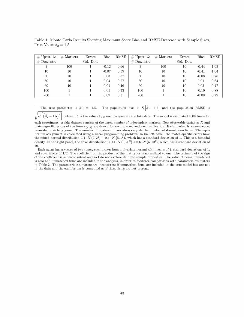
Table 1: Monte Carlo Results Showing Maximum Score Bias and RMSE Decrease with Sample Sizes,True Value β2 = 1.5

# Upstr. & # Markets Errors Bias RMSE # Upstr. & # Markets Errors Bias RMSE# Downstr. Std. Dev. # Downstr. Std. Dev.

3 100 1 -0.12 0.66 3 100 10 -0.44 1.0310 10 1 -0.07 0.59 10 10 10 -0.41 1.0430 10 1 0.03 0.37 30 10 10 -0.08 0.7660 10 1 0.04 0.27 60 10 10 0.01 0.6460 40 1 0.01 0.16 60 40 10 0.03 0.47100 1 1 0.05 0.43 100 1 10 -0.19 0.88200 1 1 0.02 0.31 200 1 10 -0.08 0.79

The true parameter is β2 = 1.5. The population bias is E[β2 − 1.5

]and the population RMSE is√

E

[(β2 − 1.5

)2], where 1.5 is the value of β2 used to generate the fake data. The model is estimated 1000 times for

each experiment. A fake dataset consists of the listed number of independent markets. New observable variables X andmatch-specific errors of the form ε〈u,d〉 are drawn for each market and each replication. Each market is a one-to-one,two-sided matching game. The number of upstream firms always equals the number of downstream firms. The equi-librium assignment is calculated using a linear programming problem. In the left panel, the match-specific errors havethe mixed normal distribution 0.4 · N

(0, 22

)+ 0.6 · N

(5, 12

), which has a standard deviation of 1. This is a bimodal

density. In the right panel, the error distribution is 0.4 ·N(0, 202

)+ 0.6 ·N

(5, 102

), which has a standard deviation of

10.Each agent has a vector of two types, each drawn from a bivariate normal with means of 1, standard deviations of 1,

and covariances of 1/2. The coefficient on the product of the first types is normalized to one. The estimate of the signof the coefficient is superconsistent and so I do not explore its finite sample properties. The value of being unmatchedis zero and unmatched firms are included in the analysis, in order to facilitate comparisons with parametric estimatorsin Table 2. The parametric estimators are inconsistent if unmatched firms are included in the true model but are notin the data and the equilibrium is computed as if those firms are not present.

43

Table 2: Comparing Maximum Score to Parametric Estimators, True Value β2 = 1.5

Maximum Score Likelihood MCMC Method of MomentsTrue Errors Number of Bias RMSE Time Bias RMSE Time Bias RMSE Time

Distribution Std. Dev. Upstream Firms (s) (s) (s)Normal 1 3 -0.16 0.54 2 -0.13 0.19 2700 0.03 0.337 1400Normal 25 3 -0.54 1.14 2 0.28 0.74 2700 -0.26 2.00 1400Normal 50 3 -0.37 1.14 2 0.49 1.86 2900 -0.14 3.54 1500Normal 1 4 -0.02 0.50 2 -0.16 0.20 7100 0.01 0.31 2100Normal 25 4 -0.42 1.13 2 -0.07 0.79 7000 -0.03 1.59 2000Normal 50 4 -0.77 1.30 2 -0.17 1.55 7000 -0.37 2.61 2100

Mixed Normal 1 3 -0.11 0.69 2 -1.19 1.19 2700 -1.09 1.10 1400Mixed Normal 25 3 -0.46 1.17 1 -0.31 1.12 2400 -0.58 1.96 1000Mixed Normal 50 3 -0.60 1.46 1 -0.33 2.27 2400 0.16 3.77 1300Mixed Normal 1 4 0.05 0.65 2 -1.13 1.13 7100 -1.07 1.07 2100Mixed Normal 25 4 -0.68 1.15 2 -0.47 0.84 7000 -0.56 1.32 2000Mixed Normal 50 4 -0.93 1.58 2 -0.16 1.26 7200 -0.57 2.61 2100

The true parameter is β2 = 1.5. The population bias is E[β2 − 1.5

], and the population RMSE is√

E

[(β2 − 1.5

)2], where 1.5 is the value of β2 used to generate the fake data. The model is estimated 100 times

for each experiment. The same fake dataset is used for all three estimators. A fake dataset consists of 100 independentmatching markets. New observable variables X and match-specific errors of the form ε〈u,d〉 are drawn for each marketand each replication. Each market is a one-to-one, two-sided matching game. The number of upstream firms alwaysequals the number of downstream firms. The equilibrium assignment is calculated using a linear programming prob-lem. Each firm has a vector of two types, each drawn from a bivariate normal with means of 1, standard deviationsof 1, and covariances of 1/2. In the top panel, the match-specific errors ε〈u,d〉 have N

(0, σ2

)distributions, where

σ is the standard deviation listed in the table. In the bottom panel, the errors have the mixed normal distribution0.4 ·N

(−6, σ2

1

)+ 0.6 ·N

(4, σ2

2

), where the total dispersion of ε〈u,d〉 is given in the table. This is a bimodal density.

Each agent has a vector of two types. For maximum score, the coefficient on the product of the first types is normalizedto one. The estimate of the sign of the coefficient is superconsistent and so I do not explore its finite sample properties.Coefficients on both parameters are estimated for the parametric estimators, as the scale normalization is on the errorterm. The coefficient estimates of the parametric estimators are multiplied by the true standard deviation of the errors,to make the scale normalization comparable to maximum score. All experiments were done on the same computer usingMATLAB. Times listed are CPU times.

44

Table 3: Specialization By Suppliers and Assemblers

Revenue Function Estimates Sample Statistics for HHI MeasuresHHI Measure Point Estimate 95% CI Mean Standard Deviation

SuppliersContinent +1 Superconsistent 0.725 0.210

Parent Group 4.09 (1.58,5.76) 0.395 0.291Brand 11.6 (3.37,18.9) 0.283 0.292Model 86.0 (75.9,132) 0.201 0.286

AssemblersParent Group -0.0698 (-0.106,-0.013) 0.312 0.196

Brand -0.0294 (-4.37,0.008) 0.449 0.204Model -0.0315 (-7.38,0.254) 0.786 0.162

# Inequalities 332,218% Satisfied 80.6%

I estimate βupCont. by optimizing the maximum score objective function over the other parameters, first fixing

βCont. = +1 and then fixing βCont. = −1. I then take the set of estimates corresponding to the maximum of the twoobjective function values as the final set of estimates. The estimate of a parameter that can take only two values issuperconsistent, so I do not report a confidence interval.

I use the numerical optimization routine differential evolution, in Mathematica. For differential evolution, I use apopulation of 200 points and a scaling factor of 0.5. The numerical optimization is run 30 times with different initialpopulations of 200 points. I take the point estimates corresponding to the maximum reported objective function valueover the 30 runs. For inference, I use subsample sizes equal to 1/4 of the matching markets. Unfortunately, the literatureon subsampling has not produced data dependent guidelines for choosing the subsample size. I use 150 replications(artificial datasets) in subsampling. Following the asymptotic theory, I sample from the 187 distinct matching markets(component categories). Constructing the inequalities, producing the 30 estimates, and constructing confidence intervalstook 9.5 hours on a single core of a 2010 vintage desktop computer.

In the maximum score objective function, an inequality is satisfied if the left side exceeds the right side by 0.0001.This small perturbation to the sum of revenues on the right side ensures that inequalities such as 0 > 0 will not becounted as being satisfied because of some numerical-approximation error resulting in, say, 2.0× 10−15 > 1.0× 10−15.

Table 4: Percentage Revenue Change By Suppliers From GM Divesting Opel

Quantile0 -0.090

0.10 -0.0280.25 -0.016

0.50 (median) -0.0070.75 -0.0030.90 -0.0011 ~0

This table uses the point estimates from Table 3 to calculate the structural revenues of suppliers before and afterGM divests Opel. In the model, Opel becomes a separate parent group. For each firm selling one or more parts to Opel

and one or more cars to another GM brand, I calculateβupPG∆z

upParentGroup(Mu)

rupβup

(Mu).

45

Table 5: Supplier Competitive Advantages From Asian Assemblers

Revenue Function Estimates Sample Statistics for HHI MeasuresHHI Measure Point Estimate 95% CI Mean Standard Deviation

SuppliersContinent +1 Superconsistent 0.725 0.210

Parent Group 4.04 (2.29,5.49) 0.395 0.291Brand 11.6 (6.68,18.8) 0.283 0.292Model 84.3 (74.3,127) 0.201 0.286

Competitive Advantage -3.20 (-4.71,-2.49) 0.069 0.160Assemblers

Parent Group -0.0940 (-0.147,-0.048) 0.312 0.196Brand -0.0219 (-2.95,0.006) 0.449 0.204Model -0.0381 (-5.08,0.216) 0.786 0.162

# Inequalities 332,218% Satisfied 80.8%

See Table 3 for implementation details.

46