Estimating labour supply elasticities based oncross-country micro data: A bridge between micro and

macro estimates?

Markus JänttiSwedish Institute for Social Research

Stockholm Universitymarkus.jantti@sofi.su.se

Jukka PirttiläSchool of ManagementUniversity of Tampere

jukka.pirttila@uta.fi

Håkan SelinUppsala Center for Fiscal Studies at the Department of Economics

Uppsala Universityhakan.selin@nek.uu.se

February 27, 2013

Abstract

We utilise repeated cross sections of micro data from several countries, available from the Lux-embourg Income Study, LIS, to estimate labour supply elasticities, both at the intensive and exten-sive margin. The benefit of the data is that it spans over four decades and includes a large number oftax reform episodes, with tax rate variation arising both from cross-sectional and country-level dif-ferences. Using these data, we investigate whether micro and macro estimates differ in a systematicway. The results do not provide clear support to the view that elasticities at the macro level wouldbe higher than corresponding micro elasticities.

JEL Classification: E24, H21, J22.

Keywords: Labour supply, earnings, taxation, cross-country comparisons.

Acknowledgments: We are grateful to seminar participants of the Conference on the Economics ofthe Nordic Model (Oslo) and Helsinki Center for Economic Research for useful comments. AllanSeuri provided excellent research assistance. Financial support from the Yrjö Jahnsson Foundationand the Finnish Employees’ Foundation is gratefully acknowledged.

1 Introduction

Much of the modern empirical evidence on the impact of taxation on labour supply and taxable incomeis based on careful examination of how individuals react to tax reforms. This type of micro-data basedevidence has been argued to plausibly identify the causal effects of tax changes on taxpayer behaviour.It is summarised by Meghir and Phillips (2010) in their chapter for the authoritative treatment of taxresearch in the Mirrlees Review. They conclude that while labour market participation decisions canbe quite elastic with respect to the take-home pay when working versus when unemployed (the ’ex-tensive margin’), the working hours of those who already work (the ’intensive margin’) are typicallyquite unresponsive to tax rates. While taxable income estimates are typically higher than estimatesof working hours responses (for a recent survey, see Saez, Slemrod, and Giertz, 2012), even taxableincome responses are typically modest; typical values for taxable income elasticities with respect to thenet-of-tax rate (=1-marginal tax rate) are around 0.2-0.5.

However, there is a large discrepancy between some of the macroeconomic work and microecono-metric evidence on the employment effects of taxation of labour income. Some macroeconomistssuggest, including the provocative paper by Prescott (2004), that tax differences explain virtually allthe differences in working hours between the US and Europe. Large elasticities are also needed forconventional macro models to match the empirical fluctuations in aggregate employment over businesscycles. Sometimes macro studies are based on simple cross-country comparisons and they do not typ-ically pay attention to endogeneity issues, such as the possibility that if the economy performs badlyand unemployment rises, countries need to raise taxes to balance budgets. And they often omit otherpotential explanatory variables that could affect employment. 1

But it is not clear either that the micro estimates provide the correct estimates of the long run effectsof taxes on labor supply behaviour, for the following reasons. There are now several recent papers thataim to explain why micro and macro estimates differ so significantly. Chetty (2012) provides the firstpossible solution building on frictions. While micro evidence has paid a lot of attention to carefullyestimating the causal effects of specific tax changes, these tax changes are often too small to generatereally large society-wide impacts. If there are frictions related to re-optimisation of labour supply andincome generation, it may not be worthwile for the individuals to react to small tax changes. Thenestimates based on micro evidence can be downwards biased, whereas the tax differences betweencountries are often so large that, in the long run at least, the economy and the individuals have reactedto those optimally. In Chetty et al. (2011a), the authors demonstrate that if taxation of householdscreates economy-wide structures, employers are likely to cater for employees’ desires by offering com-pensation packages that suit the majority of the workforce. They also provide evidence from Denmark,where many taxpayers (and in particular in occupations where compensation packages can be tailored

1Nickell (2003) concludes that when other potential explanations for employment behaviour (such as differences inwage setting frameworks and social security systems) are accounted for, a 10 percent difference in taxes on labour incomeexplains roughly 2 per cent of cross-country variation in employment rates.

1

well) bunch at income levels where they just avoid paying an increased state-level marginal tax rate.Chetty et al. (2011a) also show how smaller tax changes, which do not affect all tax payers, generatemuch smaller behavioural elasticities than a single large increase in the marginal tax rate at the countrylevel.

The second explanation is related to indivisible labour and varying responses along the intensiveand extensive margin. A key paper in this strand of research is Rogerson and Wallenius (2009), whointroduce the extensive margin to an otherwise standard macro model and demonstrate how the presenceof fixed costs generates a realistic life-cycle profile or labour supply. While taxation might not matterso much for the hours choice of the working age population, it can have a sizable impact on the lengthof the working life, so that at the aggregate level hours become quite responsive to tax changes.

The third explanation, building on Imai and Keane (2004), relies on the way human capital forma-tion interacts with taxation. In a learning-by-doing framework, taxation can have significant long-runconsequences, because if it leads to lower working hours in a current period, it also depresses wages inlater periods. Therefore the cumulative distortionary effect of taxation, which matters at a macro level,could be much higher than what a typical static micro estimate would suggest.

Finally, even if the majority of micro-level labour supply studies would imply fairly small elastici-ties at the intensive margin, some of the elasticity of taxable income studies, surveyed recently by Saez,Slemrod, and Giertz (2012), find much larger elasticities, especially at the top of the income distribu-tion. However, these elasticities capture for instance income shifting behaviour, and cannot be directlyused to predict cross-country differences in employment.2

Despite this emerging research, the issue is, however, far from settled. This is reflected in theconclusions by two recent surveys on the topic by leading researchers in the field. Chetty et al. (2012)conclude that

“Based on our reading of the micro evidence, we recommend calibrating macro models tomatch Hicksian elasticities of 0.3 on the intensive and 0.25 on the extensive margin,”

which would lead to a combined macro elasticity of approximately 0.5. In contrast, Keane and Roger-son (2012) argue that

“In our view, the literature we have described can credibly support a view that compensatedand intertemporal elasticities at the macro level fall in the range of 1 to 2 that is typicallyassumed in macro general equilibrium models.”

Since reliable evidence on the impacts of tax changes on working hours is one of the most importantknowledge economic policymakers need, there is clearly an urgent need for further research that couldhelp us understand the differences between these recommendations.

The purpose of this paper is to shed new light on this micro-macro controversy by estimating laboursupply elasticities using micro-level data from a set of different industrialised countries. Building on a

2Piketty, Saez, and Stantcheva (2011) estimate top income elasticities using macro data.

2

high-quality, harmonised and compareble data from the Luxembourg Income Study (LIS), we employthe repeated cross-section estimation method developed by Blundell, Duncan, and Meghir (1998) toestimate the elasticity of working hours and labour income (at the intensive margin) and participationat the micro level, macro level and at an intermediate level where the tax variation arises from bothcross-sectional and cross-country sources.

The value-added in the paper is the following. First, the data span over several decades and countriesand contain a large number of tax reform episodes, including major tax reforms, which means that thereis good scope for reliable estimation. Additionally, tax changes have taken place accross the incomedistribution, not only among top income earners.

Second, we use the same estimator and harmonised data to estimate micro and macro elasticities.3

We can compare if micro elasticities are in fact smaller than macro elasticities, without differencesin methodology confounding the potential differences in micro estimates from different countries ordifferences between micro and macro level reactions.

Third, at the macro level, the model is also correctly specified (from the point of view of a staticlabour/earnings supply model), since we actually use mean marginal tax rates and virtual income fromthe data, rather than artificial constructs or average tax rates. In addition, the marginal tax rate weuse also includes (in our main specifications) not only the increase in tax liability but also reductionsin transfers and benefits; that is, we use the theoretically correct effective marginal tax rates. 4 Andfourth, we provide a separate analysis of intensive and extensive margin, both estimated at the microand macro level.

The topic is of key importance to the Nordic model: The size of the public sector in the Nordiccountries is among the largest in the world, and since tax distortions, other things equal, rise with thetax rate, the burden of financing the public sector can become very large.5 On the other hand, Rogerson(2007) and Blomquist, Christiansen, and Micheletto (2010) point out how the Nordic arrangement ofsubsidising goods that are used in conjunction with labour supply (such as childcare) counteract someof the harmful effect of taxation on work effort. Our data contain key Nordic countries, and we cancompare their situation with interestingly different institutional settings, including the Anglo-Saxoncountries.

Needless to say, the study also has some limitations. We cannot cover all OECD countries, sincefor some of the countries, suitable data is not available from LIS. We control for education level in the

3We follow Chetty, citet above, and refer to macro elasticities if the source of the tax variation used in explaining laboursupply is cross country comparisons; micro elasticities refer to findings identified from cross-sectional variation within acountry

4We also compare our macro estimates to the standard ways, used earlier in the literature, to estimate country-levelresponses to taxation.

5The well-known revenue-maximising top marginal tax rate for Pareto distributed top incomes is given by the formula1/(1+ a ∗ e) where a is the Pareto Lorenz coefficient and e is the elasticity of taxable income. With a typical Nordicvalue of a equal to approximately 2, the marginal tax rate on top incomes should not exceed 20 per cent if the elasticityis as high as 2, which belongs to the interval recommended by Keane and Rogerson (2012). The existing top marginal taxrate (including commodity taxes) in Sweden is currently around 70 per cent (Pirttilä and Selin, 2011). These differencesdramatically highlight the issues at stake.

3

estimations, and therefore the impact of taxes which we measure do not contain the potential that taxchanges can lead to changes in educational attainment. Our estimates capture, however, contempora-neous effects of learning-by-doing which is reflected in increases in wage rates. Unlike country-levelstudies, we do not have access to a microsimulation model to calculate effetive marginal tax rates, andwe use data-driven semi-parametric methods to estimate marginal tax rates. However, this is also amethodological novelty, and we compare the estimated tax rates to other available information on taxsystems in these countries. Because of top coding in some countries, LIS data is not perfect for exam-ining top income elasticities, but we correct for that by imputing earnings above the 97.5th percentilebased on information on top income distribution from The World Top Income Database.6

The paper proceeds as follows. Section 2 provides a more detailed review of the existing papers onthe micro-macro differences in elasticity estimates. Section 3 presents the theoretical background andempirical methodology, while Section 4 covers the data description and marginal tax rate estimation.The estimation results are presented in Section 5, and Section 6 concludes.

2 Literature review

This section surveys the emerging literature on the micro-macro differences in labour supply / earningselasticities to understand what is the current status and whether important knowledge gaps remain.Notice that our aim is not to cover conventional microecomic estimates on labour supply or taxableincome (for surveys on these, see Meghir and Phillips (2010) and Saez, Slemrod, and Giertz (2012)).

2.1 Starting point

One of the starting points for this literature is the work by Prescott (2002, 2004). In Prescott (2004),he studies seven countries (the G-7 countries) Germany, France, Italy, Canada, United Kingdom, Japanand United States, over two time periods 1970-74 and 1993-96. The analysis contains 14 observations.Prescott departs from a standard growth model with a representative household and a representativefirm, and he parameterises the value of leisure in such a way that the average labour supply the modelgenerates matches the actual values in the data. Given this choice of preference parameter he is able toobtain predicted work hours fairly close to actual work hours in 12 out of 14 cases. He obtains a laboursupply elasticity of “nearly 3 when the fraction of time allocated to the market is in the neighbourhoodof the current U.S. level”.

Obviously, “nearly 3” sounds like a very large elasticity. However, Alesina, Glaeser, and Sacerdote(2005) show that Prescott’s choice of parameter values implies an uncompensated labour elasticity of0.77. Relatedly, Chetty et al. (2011b) plot Prescott’s data and fit a regression line to it. They thenestimate a ’Hicksian’ labour supply elasticity of 0.7 on the 14 observations. The discrepancy between

6Alvaredo, Facundo, Anthony B. Atkinson, Thomas Piketty and Emmanuel Saez, The World Top Incomes Database,http://g-mond.parisschoolofeconomics.eu/topincomes, 04/10/2012

4

the two elasticity estimates is that Prescott reports a Frisch elasticity, which depends upon the specificassumption about the utility function and the wealth-earnings ratio.7 In fact, Prescott’s functional formassumptions and choice of parameter values also imply sizable income effects on labour supply. Againstthis background, it is an interesting feature of our study that we also estimate the response to changesin unearned income (even though one should keep in mind that our static labour supply model in somerespects differs from Prescott’s model).

Prescott’s paper has given rise to a large debate. The basic conclusions were broadly supportedby Ohanian et al. (2008), who used a similar methodology. Other researchers (e.g Nickell (2003) andAlesina, Glaeser, and Sacerdote (2005)) have pointed at the difficulties of teasing apart the impact oftaxes from other factors that also affects aggregate work hours in a country. In addition, Ljungqvistet al. (2006) point out that the conclusions in Prescott (2002) change if one also considers that workerstypically receive unemployment benefits (as a certain fraction of their work income) when unemployed.

2.2 Related papers

Blundell, Bozio, and Laroque (2011) describe the long-run evolution of mean annual hours per worker,employment rate and the unconditional mean hours per individual on Labour Force Survey data fromthe US, the UK and France. Of particular interest is that total hours in the UK have decreased overa forty-year period, despite the fact that UK has adopted similar tax policy reforms as the US (e.g.in work tax credit policies). Blundell et al find that neither the intensive nor the extensive margindominates in explaining the changes in total hours worked. The relative importance of the two marginsdiffers across age, gender and family composition groups.

Davies and Henrekson (2004) exploit aggregate data for nineteen countries on outcome variablessuch as the ratio of employment to population of working age, annual hours worked per employedperson and annual hours worked per adult of working age. According to their results, average tax ratesare strongly negatively associated with working hours and employment rates in an OLS regression, butthe coefficient becomes insignificant when country fixed effects are included.

The study by Piketty, Saez, and Stantcheva (2011), while not so much related to the literature onmicro-macro elasticities, is interesting since it uses macro data to estimate taxable income elasticitiesat the top. The authors set up an optimal tax model in which top incomes respond through three chan-nels: (1) the standard labour supply response, (2) the tax avoidance channel and (3) the compensationbargaining channel through efforts in influencing own pay setting. Importantly, bargaining efforts arezero-sum in the aggregate. Therefore, the optimal tax rate increases with the bargaining elasticity.

In the empirical part, Piketty et al analyse top income and top tax rate data in 18 OECD countries.They exploit the World Top Income Database combined with top income tax rate data starting in 1975.Piketty et al. find a strong correlation between the growth in top incomes and marginal tax cuts for

7The Frisch elasticity of labour supply is derived holding marginal utility of consumption constant, whereas Hicksianestimates typically used by public finance economists are derived holding utility constant.

5

top income earners. Higher top incomes did not, however, lead to higher GDP growth. Piketty et alinterpret this pattern as consistent with low labour supply elasticities and large bargaining elasticities.

An alternative explanation to why hours have increased in the US and fallen in Europe is related tobehavioural economics, namely the Veblen effect: When people compare their income level to that oftop earners, a rise in income inequality can render people to supply more labour because of their effortto “keep up with the Joneses”. Oh, Park, and Bowles (2012) use country-level data on working hours,taxes and top income shares and show, in a model with country and year fixed effects, how increasesin top income shares are associated with increases in working hours. Moreover, taxes lose explanatorypower for working hours when the top income share is added to the regression model.

The final paper that is relevant to the current paper, and perhaps also the closest one, is Bargain,Orsini, and Peichl (2011). They have collected micro-data on work hours, wages and taxes and benefits(microsimulation) from 17 European countries and the US. For the European countries the EUROMODmicrosimulation model has been used, whereas TAXSIM has been used for the US. The motivation forthe paper is to make a large-scale international comparison of elasticities, while netting out possibledifferences due to methods, data selection and the period of investigation. To this end, Bargain et al.estimate the same structural discrete-choice labour supply model on all these data sets, with separatemodels for couples and singles. The wage elasticities vary less between the countries than previouslythought. The resulting differences are interpreted as consequences of heterogeneous preferences.

Since our paper is more related to the micro-macro differences, the Bargain et al. study and ourwork are quite complementary. There are also many significant differences in the approaches taken.For example, we use the Blundell et al. repeated cross-section estimator, whereas they build a discretechoice labour supply model that relies on cross-sectional variation for identication, and we utilise datafrom a much longer time span.

3 Data

3.1 General features and sample selection

Our data are from the Luxembourg Income Study database, LIS, which collects household- and individual-level data on household income, taxes paid and transfers received, working hours (for a subset of coun-tries) and consumption (Luxembourg Income Study Database (LIS), 2012). The benefit of the data isthat LIS has invested a large amount of work to make the data comparable across countries and acrossyears.8 LIS provides income, labour market, and demographic data that have been harmonised in toa common template, so the contents of the variables are as comparable as cross-country data, acrosstime, can get.

8For information on data harmonization, see http://www.lisdatacenter.org/wp-content/uploads/our-lis-documentation-harmonisation-guidelines.pdf.

6

Another benefit of the data is that it spans over four decades; the data we use start from the beginningof the 1970s. It also covers a wide range of different type of countries; we focus on developed (OECD)countries. Not all information is available for all countries, however. The main dividing line is between’gross’ and ’net’ data sets. Gross data sets record all market and non-market income sources grossof income taxes, whereas net data, as the name suggests, include only information on income sourcesnet of taxes withheld. We can, of course, use only those countries that provide gross data, in LISparlance. In addition, even if household-level data exist, individual-level earnings data are not alwaysavailable. These restrictions limit the number of countries we cover to 13. These include, most notably,key Anglo-Saxon countries (the US, the UK, Australia), the Scandinavian countries, and some CentralEuropean countries (such as Germany and Netherlands). 9 The countries in our data are interestinglydifferent in their institutional characteristics and the role and size of the government in the economy.

As mentioned in the introduction, the data are repeated cross sections from a number of waves.The exact year corresponding to a particular wave varies somewhat across countries. Table 1 lists thecountries and years in our data.

We have three key dependent variables in our empirical analysis: annual work hours, earnings andlabour force participation. The variable for annual work hours is created from survey questions onweekly hours and number of weeks worked per year. We can use information on work hours for sevencountries: Australia, Canada, Germany, Netherlands, Sweden, U.K and U.S. 10

The earnings variable, which is available for all 13 countries, includes both monetary and non-monetary compensation. For a majority of countries, the earnings variable comes from surveys, butfor some countries, especially the Nordic ones, it is based on register data. Using earnings as thedependent variable captures the effects of taxes on effort that is reflected in changes in the hourly wagerate (Feldstein, 1995). Notice, however, that in contrast to the taxable income literature, our earningsmeasure is not necessarily taxable labour income, since it is not net of tax deductions.

We have limited our analysis to four types of households, single persons (with and without children)and couples (again, with and without children) to be able to more cleanly estimate how taxes andtransfers vary with income.11 The estimation samples for the intensive margin analysis (work hoursand earnings) and the extensive margin analysis are selected in slightly different ways. We impose thefollowing restrictions on the ’intensive margin sample’. First, we only include individuals aged 25-54,so that retirement is not an issue. Second, we exclude individuals who earn less than the 20th percentile,where percentiles are defined based on the distribution of earnings in country c in period t. 12

In the extensive margin analysis, we include all individuals aged 25-64 in the sample. In the ex-

9Prior to 1990 West Germany was a LIS country. For the post-1990 samples for re-unified Germany, we excluded theformerly East German Länder.

10We also have hours data for Finland in 1991 and Belgium in 1997. However, as the estimation framework builds onchanges in taxes across time and groups we leave Finland out from the hours regressions.

11This means that we exclude households that include adults that are not in the nuclear family.12It is common in the empirical tax literature to impose a lower income limit on the estimation sample, see e.g. Gruber

and Saez (2002)

7

tensive margin analysis, it is in fact desirable to also capture the retirement margin (as emphasised byRogerson and Wallenius, 2009).

Some of the LIS data sets are top coded, which is problematic because then the mean income amonghigh income earners is downwards biased. Since in many countries, especially the US and the UK, taxreductions have been focused on high income earners, and their incomes have risen faster than others’income, if we did not correct top coding, we could have downwards biased estimates for these taxepisodes. For this reason, we replace the incomes above the 97.5 percentile with random draws fromPareto distribution, the parameters for which are available from the World Top Income Database.13

The model below in Section 4 lays out in more detail the requirements of the empirical model. Interms of data, we also need information on capital income. Demographic variables (sex, education,age, household type) are also used.

3.2 Tax variables

A key variable in the intensive margin analysis is the effective marginal tax rate. 14 The slope of theindividual’s budget constraint is not only determined by the statutory income tax schedules, but also bythe transfer systems in place. To our knowledge, there is no microsimulation model that can be usedto compute effective marginal tax rates for all the countries in all the years oin our data. We thereforeproceed in the following way. For the purpose of calculating the statutory income tax schedules, webuild a small tax calculator. For a majority of countries we exploit information on segment limits andrates (for both central government and subcentral government taxation) provided by the OECD from1981 and onwards. 15 The OECD information applies to singles without dependents. For countries andtime periods where the OECD information is missing or insufficient, we have collected informationfrom alternative sources, e.g. from the library of the International Bureau of Fiscal Documentation(IBFD) in Amsterdam and the European Tax Handbooks, various editions. The coded tax functions arethen used to compute marginal tax rates, taking into account differences between joint vs. individualtaxation and global vs. dual income taxation.

Needless to say, the tax rates calculated in this way are not ideal measures of the individuals’marginal incentives to earn income. A limitation of our data is that information on deductions areabsent. As mentioned above, we do not observe taxable income net of deductions, which is the relevantbase for income taxation. As a consequence, given that marginal tax rates typically are increasing in

13Since the parameters are estimated for total market income, they could be slightly overestimated for the earningsdistribution we use. This needs to be kept in mind when examining the results for earnings.

14Our measure of taxes does not include social security payments. One reason for this choice is that while the data hashousehold or individual level information on the social security payments made by the employees, the social security pay-ments paid by the employers would need to be imputed. Countries also differ significantly in the division of these paymentsbetween employees and employers, and this division should not really matter for tax incidence. For equal treatment of coun-tries, we decided not to take these payments into account.For macro regressions, we also calculate alternative tax functionsthat take into account proportional payroll taxes and consumption taxes. The rates of these vary only at the country level.

15This information is available at http://www.oecd.org/tax/taxpolicyanalysis/oecdtaxdatabase.htm#pir.

8

Table 1 Countries and years of dataCountry YearsAustralia 1985(h), 1989(h)Belgium 1992, 1997(h)Canada 1981, 1987(h), 1991(h), 1994(h), 1997(h),1998(h), 2000(h), 2004(h)Czech republic 1996, 2004Denmark 1987, 1992, 1995, 2000, 2004Finland 1987, 1991(h), 1995, 2000, 2004Germany 1984, 1989(h), 1994(h), 2000(h), 2004(h)Israel 1992, 1997, 2001, 2005Netherlands 1987, 1999(h), 2004(h)Norway 1986, 1991, 1995, 2000, 2004Sweden 1992(h), 1995(h), 2000, 2005United Kingdom 1991(h), 1995(h), 1999, 2004United States 1974(h), 1986(h), 1991(h), 1994(h), 1997(h), 2000(h), 2004(h)

Note: (h) indicates availability of data on annual work hours.

income, we believe that the true level of statutory marginal tax rates facing taxpayers is lower than theone we have calculated.

It is considerably more challenging to collect information on the transfer systems for all coun-tries/years. For the purpose of calculating the marginal effects arising from the transfer systems wetherefore suggest a data-driven approach, where we fit a non-parametric regression on labour incometo predict marginal effects. We use the locfit package in R to carry out these regressions (For informa-tion on these estimation techniques, see Chapter 6.1 in Loader, 1999). The procedure estimates localpolynomial regressions, regressing taxes on income; the first derivative of the estimates then representsthe marginal rate of transfer withdrawal as earnings increase. The benchmark regressions use a thirddegree polynomial, a nearest-neighbour bandwidth of 0.7 (that is, 70 per cent of observations are usedat every evaluation point) and a Gaussian weighting function. We also experimented with alternativebandwidths and polynomial degrees.

Figure 1 depicts an example of marginal tax rates and effective marginal tax rates used in theanalysis. Note that the shape of these two functions are completely different: marginal tax rates aremonotonically increasing, whereas it is well known that effective marginal tax rates take a U shapedform: they are highest at the bottom of the income distribution because of tapering off of benefits.This means that the real incentives, taking into account transfer systems, can be completely different tomany individuals than a typical analysis, using solely statutory taxes, would suggest.

For the extensive margin analysis we are interested in participation tax rates rather than marginaltax rates. These are obtained by making use of the same combination of coded statutory tax functionsand local polynomial regressions of transfers as a function of income (evaluated at zero hours of workand at an imputed earnings level, see more below).

9

Figure 1 Marginal and effective marginal tax rates, Finland and Sweden 1995-2004A. Finland

Labor earnings (real 2010 USD PPP dollars)

τ statut

ory

0.2

0.4

0.6

0.8

20000 40000 60000

MTR

20000 40000 60000

EMTR

1995 2000 2004●

B. Sweden

Labor earnings (real 2010 USD PPP dollars)

τ statut

ory

0.0

0.5

1.0

1.5

0 20000 40000 60000 80000 120000

MTR

0 20000 40000 60000 80000 120000

EMTR

1995 2000 2005●

10

4 Empirical model

4.1 Basic model

As mentioned above, our aim is to utilise micro data from several countries and several time periodsto estimate both ’micro’ and ’macro’ elasticities using the same data source. Following Chetty et al.(2011b), we use the terms ’micro’ and ’macro’ elasticities to refer to the sources of variation used toestimate the elasticities. When the elasticity is identified based on quasi-experimental variation betweendifferent groups in a single country we refer to the estimated elasticity as a ’micro’ elasticity. Whenthe elasticity is identified by cross-country and time variation, the estimated elasticity is a ’macro’elasticity.

In this section, we elaborate on how to estimate micro elasticities for a single country. Even thoughwe only have information on work hours for a subset of countries, we nevertheless find it natural tostart to discuss intensive margin hours responses. We start off from the standard static labour supplymodel, where individuals maximise the utility function U =U(c,h) with respect to consumption, c, andlabour supply in terms of annual hours, h, subject to the linearised budget constraint c = (1−τ)wh+R,where w is the gross hourly wage rate, τ is the marginal tax rate and R is virtual income. Virtual incomecan be computed as R = m+ τz−T (z), where m is non-labour income (e.g. the income of the spouseand capital income), z = wh, and T (z) is the income tax function. 16 The hourly wage rate has beenobtained by dividing annual earnings by annual hours. In accordance with e.g. Blundell, Duncan, andMeghir (1998), we assume the following labour supply function;

hit = β ln(1− τit)wit + γRit + εit , (1)

where i is an individual index and t is a time index. The uncompensated labour supply elasticity incountry c (evaluated at mean hours in country c) is given by β/h , where h is mean hours in countryc.17 The equation is estimated on all i who supply positive hours.

Suppose that we were to estimate equation 1 by OLS. As both of the right-hand side regressorsare correlated with ε and so are endogenous, estimates of both of the parameters are biased. Themost obvious reason is that both τ and R are direct functions of z = wh. An additional reason is thatunobserved variables (e.g., tastes for work and savings) might affect work hours h, the gross wage ratew and the level of non-labour income m simultaneously.

The repeated cross section element of our data allow us to compare groups of individuals overtime and, thereby, adress these endogeneity issues by constructing instruments. Following Blundell,

16 The virtual income consists of the individual’s non-labour income and a term that takes into account that inframarginalunits of supplied income is taxed at other rates (typically lower rates) than income supplied at the margin. Formally, for ageneral nonlinear tax system T (z), virtual income at a point x is defined as the intersection between the tangent (i.e linearapproximation) of the budget set c(z) = z−T (z) at x and the consumption axis.

17The compensated labour supply elasticity, which is the relevant parameter for deadweight loss calculations, can beobtained through the Slutsky relationship.

11

Duncan, and Meghir (1998), we partition the sample into group cells based on country, gender, ageand education level. They key idea behind the grouping procedure is to compare otherwise similargroups of individuals who have been affected differently by tax reforms (the difference-in-differenceidea) while retaining the ambition to estimate structurally meaningful parameters (in this case β and γ).

Let g denote group cell. Suppose that εit = αg +µt +ηit , where E[ηit |hit > 0,g, t] = 0. Accordingto this assumption unobserved heterogeneity, conditional on g and t, can be captured by a permanentgroup effect αg and a time fixed effect µt . This assumption can also be modified in such a way thatit allows e.g. for education group specific linear time trends. Let qgt be a vector that contains the fullset of interactions between group and time. By assumption, these are uncorrelated with ηit . This is thecentral exclusion restriction for identification. We can then estimate

hit = β ln(1− τit)wit + γRit +αg +µt +ηit (2)

by two-stage least squares (2SLS) while using qgt as excluded instruments for ln(1− τit)w and Rit .Crucially, both the order condition and the rank condition for identification need to hold. The ordercondition requires us to have at least as many instruments as endogenous regressors (in our case, two).The rank condition requires that net wage rates and virtual incomes must both change at different ratesfor different groups over time. As the variation in the second stage equation is entirely at the grouplevel, equation (2) can also be estimated by collapsing the data into time-specific group averages of therelevant variables.18 We then estimate

hgt = βmicroln(1− τgt)wgt + γmicroRgt +αg +µt +ηgt (3)

by GLS, using group size as weights. Using either equation (2) or (3) yields identical results.One should recognise that tax reforms are not the sole source of identifying variation when estimat-

ing (3). Identification also comes from differential growth in gross hourly wage rates.

4.2 Macro elasticities

We will now highlight the country-time dimension of our data. Equation 2 can also be estimated by2SLS using the interactions between the country dummies and time dummies as excluded instruments.Let c be a country index and let αc be a country-specific fixed effect. The macro elasticity can beestimated by collapsing the data into year-specific country averages and running the regression

hct = βmacro ln(1− τct)wct + γmacroRct +αc +µt +ηct (4)

Since it is common in the macro literature not to weight by country size, we estimate (4) by OLS ratherthan GLS as a baseline. Thus, we let the weights within each country sum to one. The results from

18 See Angrist and Pischke (2008, section 4.1.3.) for an interesting discussion about IV estimation on grouped data.

12

those regressions can be readily compared with earlier macro-level regressions.

4.3 Micro-macro estimates

A third alternative, which can be characterised as a bridge between micro and macro estimation, is touse micro data for several countries in the same regression. While retaining the above notation, wewrite the regression equation as

hgct = βmicromacro ln(1− τgct)wgct + γmicromacroRgct +αcg +µt +ηgct , (5)

which we estimate by GLS. To achieve comparability with the macro regressions, we normalise theweights in such a way that they sum to 1 for country c in year t. The elasticity is now identified byvariation both between groups (defined by sex, age and education) and between countries.

One can add additional controls, such as country-specific trends to this equation. In this case, theequation above is rewritten as εit = αg + µt + δc× trend +ηit . In words, unobserved heterogeneity,conditional on g and t, can be captured by a permanent group effect αg, a time fixed effect µt and acountry-specific linear time trend, δc× trend. Education-specific trends can be added in similar spirit.

The practical complication that arises in the estimations is that we need to take into account spousalincome in the regressions, and countries have different solutions to family taxation (joint vs individualtaxation). Also, capital income is treated in different ways (income taxation can either be comprehen-sive or then capital income is taxed using a different schedule, as in a dual income tax). In AppendixA, we describe the way budget constraints, including virtual income, are calculated for these differentcases.

4.4 The extensive margin

The analysis above was limited to the reaction at the intensive margin (for those who supply a positiveamount of hours). We now model separately the individual’s decision whether or not to work. Inthe extensive margin model, each individual chooses between two points in the consumption-earningsspace. They choose between consumption at zero earnings and at the earnings level they potentiallywould earn if they entered the labour market.

Following e.g. Immervoll et al. (2007), suppose the utility when working takes a quasi-linear formU = c− v(z), where v(z), v(0) = 0, reflects the disutility of earnings supply.19 Let the subscripts w

and nw denote consumption and earnings in the state of work and non-work, respectively. The utilityfrom not working is just cnw. Therefore, the individual works if cw− cnw > v(zw). Consumption whenworking is given by cw = zw−T (zw)+q where T (z) denotes the transfers received and taxes paid and

19 v(z) can be interpreted broadly to also accomate fixed costs of working. To ease notation we leave the term capturingthe fixed costs out.

13

q other household income. Consumption when not working is cnw = −T (0)+ q. The condition forworking can therefore be written in terms of tax variables as

zw− [T (zw)−T (0)]− v(zw)> 0 (6)

which can also be written as(1−a)zw− v(zw)> 0 (7)

where a = [T (zw)− T (0)]/zw is the participation tax rate, i.e. the increase in taxes and the loss inbenefits, relative to gross earnings, when the individual starts to earn positive labour income. For linearprobability models, the empirical counterpart of equation (7), the probability to work P(work)i,t for theindividual i and at period t is20

P(work)it = α+βext ∗ (1−ait)zw,it + εit , (8)

where P(work) is defined to take on the value of 1 if the individual supplies earnings exceeding zero.The participation elasticity, i.e. the percentage change in the probability to work from a percentagechange in 1−a, can be calculated as βext× [(1−a)z/P(work)]. In similarity with the hours regressions,identification of β does not only rely on the tax variable a, but also on imputed potential earnings in thestate of work.

Similarly to the intensive margin case, we assume that the error term takes the form εit = αg +µt +

ηit , where E[ηit ] = 0. Equation 8 could be estimated by 2SLS using the interaction between the groupand time dummies as instruments for (1−ait)zw,it . Equivalently, one can estimate the group-averagedequation.

P(work)gt = βext(1−agt)zgt +αg +µt +ηgt (9)

by GLS.As in the intensive margin case, the analysis can also be conducted at the macro level, aggre-gating equation (9) to country level.

There are two main challenges involved in estimating the financial gain of working, (1− ait)zw,it :imputing earnings in the state of work and estimating the tax and transfer function. In Appendix B,we elaborate more on how we do this. Potential earnings in the state of work is imputed by regressingearnings on the cell dummies for those who have positive earnings.

4.5 Earnings regressions

We have also estimated how earnings respond to changes in marginal tax rates using the same estimationprocedures. Following Gruber and Saez (2002), we depart from a model where individuals maximise

20Formally, this derivation assumes that v(z) is uniformly distributed. It would perhaps have been more realistic to assumea normal distribution and, hence , arrive at a probit model. This would not, however, have been tractable from a statisticalpoint of view owing to the incidental parameter problem.

14

utility U =U(c,z) with respect to consumption, c, and taxable income supply, z, (the individual derivesdisutility from earning income) subject to the linearised budget constraint c = (1− τ)z+R, where τ,once more, is the marginal tax rate and R is virtual income. Following earlier studies on taxable incomeelasticity (e.g. Blomquist and Selin, 2010; Kleven and Schultz, 2012), we assume that the incomesupply function z = z(1−τ,R) is of the form z = (1−τ)βRγ . After taking logs and adding a stochasticterm, ε , we arrive at the regression equation

lnzit = β ln(1− τit)+ γ lnRit + εit (10)

where, as earlier, i is an individual index and t is a time index. β reflects the uncompensated earningselasticity with respect to the net-of-tax share and γ is the taxable income elasticity with respect to virtualincome. The equation is estimated on all i for which lnz exceeds the earnings threshold described inSection 3.1.

It is not unproblematic to apply the Blundell, Duncan, and Meghir (1998) estimator to earningsresponses. 21 A key distinction between the earnings and hours regressions is that the gross hourly wagerate enters the dependent variable in the earnings regressions. In the hours regressions, on the otherhand, it enters the net wage rate on the right-hand-side of the regression equation. As a consequence, theidentifying assumptions become stronger. Suppose that, for reasons unrelated to taxation (e.g. changesover time in the returns to schooling), gross wage rates grow differentially over time in different cells.In the earnings regressions, this would pose a huge threat to identification. In the hours regressions, incontrast, the same wage growth would be exploited, along with the tax changes, to identify the relevantbehavioral parameters.

5 Results

5.1 Working hours

The results on working hours are only available for seven countries for which at least two cross sectionsof data on hours are available. The country-specific estimates for all individuals, as well as men andwomen separately, corresponding to equation (3), are presented in Table 2. Various specifications of themacro level hours estimation results, corresponding to equation (4), are presented in Table 3, whereasthe micro-macro estimates of equation (5) are in Table 4. Throughout the results section, we reportelasticities rather than regression coefficients. For work hours, we report the (uncompensated) hourselasticity with respect to the net wage and the hours elasticity with respect to (virtual) non-labour

21 The typical way to proceed in the taxable income literature (surveyed by Saez, Slemrod, and Giertz, 2012) is to thetake the first difference of both sides of equation (10) and to construct instruments based on income information for thesame individuals from other years. This, however, requires panel data, which we do not have. To our knowledge, Burnsand Ziliak (2012) is the only paper which so far has explored the Blundell et al estimator in the context of taxable incomeestimation.

15

income. Reported standard errors have been obtained by the delta method.The results from countrywise regressions indicate that the elasticities are either imprecisely esti-

mated (non-significant) and, if they are significant, they are of reasonable size (such as 0.2-0.3). For 4out of 7 countries (Australia, Netherlands, Sweden and the UK) we only have two years of hours data.For these countries, it might be too optimistic to identify both the net wage elasticity and the virtualincome elasticity.

Let us now turn to the macro regressions for hours reported in Table 3. These regressions contain26 observations that are aggregates of the cells used in the micro regressions. 22 Needless to say, thesmall number of observations imposes limitations on the statistical analysis. In the specification withboth country and year dummies (column 4), the net wage elasticity is estimated to be as large as a largeas 0.641, and the estimate is significant at the 5 percent level. Remember that identification comes fromthe interaction between country and year. When we allow for heterogenous responses for males andfemales (columns 5 and 6) we obtain a higher point estimate for males.

If leisure is a normal good, we expect supply of hours to decrease when non-labour income in-creases. However, the estimated virtual income elasticities take on the ’wrong’ sign, but they are notstatistically significant.

In Table 4, we report estimates from the micro-macro regressions, where we exploit both cross-country and cell level variation for identification. In column 2, where we include both the full set ofyear dummies and country dummies, the net wage elasticity is estimated to be 0.38. When we controlfor the share of a certain household type in the cell and for education-group-specific linear time trends,very little happens to the estimated net wage elasticity. On the other hand, the virtual income elasticitygrows in the ’wrong’ direction.23 Across all specifications, the net wage estimates are significant ata level of one percent. In column 4, we report results from a specification where we control for thecountry-time variation by including interaction terms for country and year dummies. As expected,in this regression the elasticity estimate falls – it falls by 8 percentage points. This suggests that themicro-macro hours are driven both by within-country and cross-country variation.

5.2 Participation

Results on participation are derived from estimating equation (6). We present those in the form ofa participation elasticity, i.e. the elasticity of the probability to have positive earnings with respectto an increase in the difference of disposable income when in work versus when not working. Notethat income when not working contains an average income of the type of person in question whenout of work, and it also includes pension income. Thus, the participation elasticities also capture theretirement margin to some extent.

22In the micro regressions we exclude cells that contain less than 50 observations. These are, however, included whenconstructing the aggregated macro sample.

23We have defined four household types: couples with kids, couples without kids, singles with kids and, finally, singleswithout kids.

16

Tabl

e2

Cou

ntry

wis

eho

urs

regr

essi

onre

sults

A.A

llB

.Men

C.W

omen

Aus

tral

iaN

etw

age

elas

ticity

0.61

2**

0.28

1V

irtu

alin

com

eel

astic

ity-0

.148

0.10

3N

rofc

ells

33C

anad

aN

etw

age

elas

ticity

0.38

1***

0.04

8V

irtu

alin

com

eel

astic

ity-0

.135

*0.

077

Nro

fcel

ls12

6G

erm

any

Net

wag

eel

astic

ity0.

105

0.06

5V

irtu

alin

com

eel

astic

ity0.

047

0.07

7N

rofc

ells

70N

ethe

rlan

dsN

etw

age

elas

ticity

0.24

9***

0.06

3V

irtu

alin

com

eel

astic

ity0.

115

0.08

8N

rofc

ells

33Sw

eden

Net

wag

eel

astic

ity0.

240

0.16

9V

irtu

alin

com

eel

astic

ity-0

.267

0.41

8N

rofc

ells

36U

nite

dK

ingd

omN

etw

age

elas

ticity

-2.8

35*

1.36

7V

irtu

alin

com

eel

astic

ity-0

.861

**0.

362

Nro

fcel

ls25

Uni

ted

Stat

esN

etw

age

elas

ticity

0.28

0***

0.02

9V

irtu

alin

com

eel

astic

ity-0

.046

0.04

0N

rofc

ells

126

Aus

tral

iaN

etw

age

elas

ticity

1.25

4.

Vir

tual

inco

me

elas

ticity

0.85

6.

Nro

fcel

ls17

Can

ada

Net

wag

eel

astic

ity0.

403*

**0.

044

Vir

tual

inco

me

elas

ticity

-0.3

20**

0.11

9N

rofc

ells

63G

erm

any

Net

wag

eel

astic

ity0.

033

0.09

3V

irtu

alin

com

eel

astic

ity-0

.026

0.14

4N

rofc

ells

36N

ethe

rlan

dsN

etw

age

elas

ticity

0.40

70.

766

Vir

tual

inco

me

elas

ticity

-0.1

910.

085

Nro

fcel

ls18

Swed

enN

etw

age

elas

ticity

0.25

10.

156

Vir

tual

inco

me

elas

ticity

-0.5

990.

639

Nro

fcel

ls18

Uni

ted

Kin

gdom

Net

wag

eel

astic

ity-4

.593 .

Vir

tual

inco

me

elas

ticity

-1.0

66 .N

rofc

ells

13U

nite

dSt

ates

Net

wag

eel

astic

ity0.

239*

**0.

064

Vir

tual

inco

me

elas

ticity

-0.0

140.

082

Nro

fcel

ls63

Aus

tral

iaN

etw

age

elas

ticity

0.23

3.

Vir

tual

inco

me

elas

ticity

-0.3

66 .N

rofc

ells

16C

anad

aN

etw

age

elas

ticity

0.16

7**

0.07

8V

irtu

alin

com

eel

astic

ity-0

.070

0.09

2N

rofc

ells

63G

erm

any

Net

wag

eel

astic

ity0.

160

0.11

0V

irtu

alin

com

eel

astic

ity-0

.099

0.16

8N

rofc

ells

34N

ethe

rlan

dsN

etw

age

elas

ticity

-0.8

79 .V

irtu

alin

com

eel

astic

ity-3

.668 .

Nro

fcel

ls15

Swed

enN

etw

age

elas

ticity

0.46

20.

402

Vir

tual

inco

me

elas

ticity

-2.4

863.

362

Nro

fcel

ls18

Uni

ted

Kin

gdom

Net

wag

eel

astic

ity-9

.708 .

Vir

tual

inco

me

elas

ticity

-0.3

93 .N

rofc

ells

12U

nite

dSt

ates

Net

wag

eel

astic

ity0.

235*

**0.

069

Vir

tual

inco

me

elas

ticity

0.09

30.

080

Nro

fcel

ls63

Not

e:D

epen

dent

vari

able

:an

nual

wor

king

hour

s.C

ells

are

defin

edba

sed

onag

e,ed

ucat

ion

and

sex.

Cel

lsw

ithle

ssth

an50

obse

rvat

ions

are

excl

uded

.In

divi

dual

sw

ithea

rnin

gslo

wer

than

the

20th

perc

entil

ein

each

coun

try/

year

are

excl

uded

from

the

unde

rlyi

ngda

ta.

The

repo

rted

estim

ates

are

the

elas

ticiti

esof

wor

king

hour

sw

ithre

spec

tto

(1-e

ffec

tive

mar

gina

ltax

rate

)*gr

oss

hour

lyw

age

and

virt

uali

ncom

e.A

llre

gres

sion

sco

ntai

nce

lldu

mm

ies,

year

dum

mie

s,ho

useh

old

type

cont

rols

and

linea

redu

catio

ngr

oup

tren

ds.

Stan

dard

erro

rsre

port

edbe

low

the

estim

ates

are

robu

stto

hete

rosc

edas

ticity

.*

indi

cate

ssi

gnifi

canc

eat

10%

leve

l,**

5%le

vela

nd**

*at

1%le

vel.

Sour

ce:A

utho

rs’e

stim

atio

ns.

17

Tabl

e3

Hou

rsm

acro

regr

essi

ons

(1)A

ll(2

)All

(3)A

ll(4

)All

(5)M

en(6

)Wom

enN

etw

age

elas

ticity

0.19

0***

0.27

5***

0.42

1***

0.64

1**

0.51

9*0.

468

0.02

80.

036

0.08

00.

174

0.20

20.

246

Vir

tual

inco

me

elas

ticity

-0.1

430.

193

0.01

90.

703

0.39

60.

396

0.10

20.

258

0.11

70.

374

0.31

70.

495

N26

2626

2626

26Y

eard

umm

ies

No

Yes

Yes

Yes

Yes

Yes

Cou

ntry

dum

mie

sN

oN

oN

oY

esY

esY

es

Not

e:D

epen

dent

vari

able

:av

erag

ean

nual

wor

king

hour

sat

the

coun

try

leve

l.In

divi

dual

sw

ithea

rnin

gslo

wer

than

the

20th

perc

entil

ein

each

coun

try/

year

are

excl

uded

from

unde

rlyi

ngda

ta.T

here

port

edes

timat

esar

eth

eel

astic

ities

ofw

orki

ngho

urs

with

resp

ectt

o(1

-eff

ectiv

em

argi

nalt

axra

te)*

gros

sho

urly

wag

ean

dvi

rtua

linc

ome.

Stan

dard

erro

rsre

port

edbe

low

the

estim

ates

are

robu

stto

hete

rosc

edas

ticity

.*

indi

cate

ssi

gnifi

canc

eat

10%

leve

l,**

5%le

vela

nd**

*at

1%le

vel.

18

Tabl

e4

Hou

rsm

icro

-mac

rore

gres

sion

s(1

)All

(2)A

ll(3

)All

(4)A

ll(5

)Men

(6)W

omen

Net

wag

eel

astic

ity0.

275*

**0.

380*

**0.

379*

**0.

300*

**0.

406*

**0.

276*

**0.

010

0.03

40.

032

0.03

20.

050

0.05

3V

irtu

alin

com

eel

astic

ity-0

.296

***

0.02

80.

074*

-0.0

100.

109*

0.10

9*0.

019

0.04

20.

041

0.04

20.

064

0.05

6N

rofc

ells

449

449

449

449

228

221

Yea

rdum

mie

sN

oY

esY

esY

esY

esY

esC

elld

umm

ies

No

Yes

Yes

Yes

Yes

Yes

Hou

seho

ldty

peN

oN

oY

esY

esY

esY

esL

inea

redu

catio

ntr

end

No

No

Yes

Yes

Yes

Yes

Yea

r*co

untr

yN

oN

oN

oY

esN

oN

o

Not

e:D

epen

dent

vari

able

:an

nual

wor

king

hour

s.C

ells

are

defin

edba

sed

onag

e,ed

ucat

ion,

sex

and

coun

try.

Cel

lsw

ithle

ssth

an50

obse

rvat

ions

are

excl

uded

.In

divi

dual

sw

ithea

rnin

gslo

wer

than

the

20th

perc

entil

ein

each

coun

try/

year

are

excl

uded

from

the

unde

rlyi

ngda

ta.T

here

port

edes

timat

esar

eth

eel

astic

ities

ofw

orki

ngho

urs

with

resp

ectt

o(1

-eff

ectiv

em

argi

nalt

axra

te)*

gros

sho

urlty

wag

ean

dvi

rtua

lin

com

e.St

anda

rder

rors

repo

rted

belo

wth

ees

timat

esar

ero

bust

tohe

tero

sced

astic

ity.

*in

dica

tes

sign

ifica

nce

at10

%le

vel,

**5%

leve

land

***

at1%

leve

l.

19

The results from Table 5 indicate that the participation elasticities range from 0-0.4 for all individ-uals, with some that are not statistically significantly different from zero. In contrast to the intensivemargin analysis, we find that women’s elasticities are typically higher than men’s elasticities. Both thisobservation and the size of the estimates are well in line with the existing estimates in the literature.24

The macro-level participation elasticity in the ideal specification with the full set of year dummiesand country fixed effect, reported in Table 6, is actually negative, although not statistically significantlydifferent from zero. However, one needs to remember that the number of observations in the country-level regressions is quite limited (albeit larger than in many earlier papers), and the results thereforeneed to be interpreted cautiously. Nevertheless, these results indicate that macro-level participationelasticities do not appear to be greater than corresponding elasticities at the micro level, even whentaking into account the retirement margin, affecting the length of the working life. As reported incolumn 5, we have also estimated the model on the smaller sample that was used in the hours analysis,where we obtained a significant intensive margin elasticity.

When identification arises both from cross-country and cross-sectional sources (see Table 7), theestimate is always statistically significant, very modest for men but around 0.4 for women. In the mostpreferred specification (reported in column 3), the participation elasticity amounts to 0.107, and it isonly slightly larger when we instead estimate the model on the smaller sample that was used in theintensive margin analysis.

When we add interaction terms for country and year, we actually obtain a larger (and highly sig-nificant) elasticity estimate of 0.175. At first sight, this is a surprising result, because it means that weestimate a lower elasticity when we exploit cross-country variation. However, remember that in themacro analysis for the participation margin (reported in Table 6), we obtained insignificant negativeestimates of the participation elasticity. This was not the case in the hours regressions.

5.3 Earnings

As mentioned in the empirical section, the identifying assumptions in the earnings regressions are moredemanding than in the hours/participation analysis, where the earnings level was also allowed to affectthe estimates. Since earnings data are available for all countries in data set, it is of interest to brieflyreport also the earnings estimates.

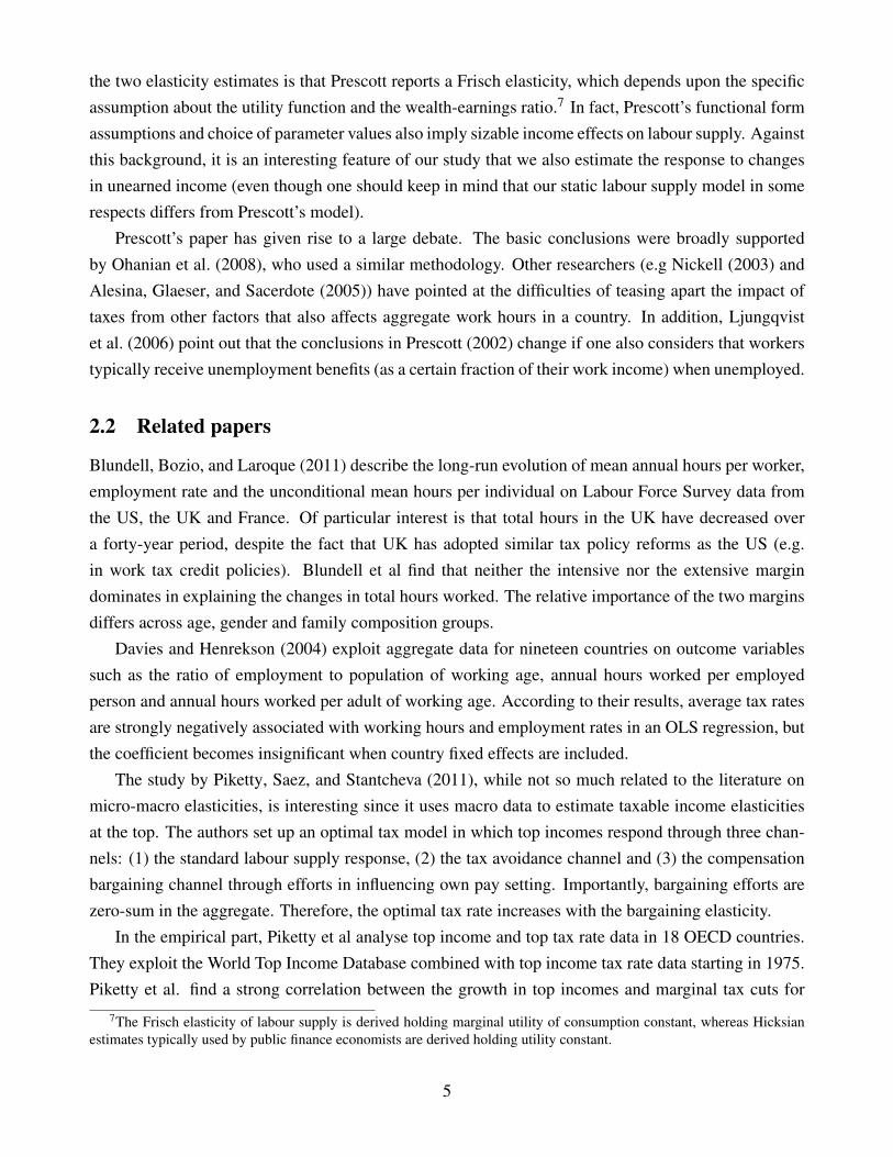
The country-wise estimates of equation (10) are presented in Table 8. Many of the estimates arenot significantly different from zero. Some have an odd negative sign for the net of tax rate; perhapsbecause the estimator we use is not very well suited for the analysis of taxable income /earnings. Themacro-level estimates are not significant, and the micro-macro estimates tend to repeat the pattern ofmicro estimates with negative signs for the net of tax rate. The macro estimate of elasticity of earningswe obtain is not greater than typical country-level estimates of e.g. elasticity of taxable income. But,

24For each country, we have also estimated specifications with household type dummies and education trends added;these alterations did not change the qualitative results.

20

Table 5 Countrywise participation regressionsA. All B. Men C. Women

AustraliaFinancial gain from work 0.366***

0.098Nr of cells 46

BelgiumFinancial gain from work 0.231**

0.094Nr of cells 48

CanadaFinancial gain from work 0.297***

0.054Nr of cells 192

Czech RepublicFinancial gain from work 0.015

0.053Nr of cells 48

DenmarkFinancial gain from work 0.205***

0.051Nr of cells 120

FinlandFinancial gain from work 0.359***

0.062Nr of cells 120

GermanyFinancial gain from work 0.189**

0.087Nr of cells 120

IsraelFinancial gain from work 0.172***

0.047Nr of cells 96

NorwayFinancial gain from work -0.008

0.012Nr of cells 120

NetherlandsFinancial gain from work 0.237***

0.077Nr of cells 67

SwedenFinancial gain from work 0.273***

0.063Nr of cells 96

United KingdomFinancial gain from work 0.329***

0.100Nr of cells 85

United StatesFinancial gain from work 0.147***

0.041Nr of cells 168

AustraliaFinancial gain from work 0.161

0.122Nr of cells 24.

BelgiumFinancial gain from work 0.222**

0.083Nr of cells 24

CanadaFinancial gain from work 0.218***

0.049Nr of cells 96

Czech RepublicFinancial gain from work 0.072**

0.025Nr of cells 24

DenmarkFinancial gain from work 0.054*

0.031Nr of cells 60

FinlandFinancial gain from work 0.250**

0.099Nr of cells 60

GermanyFinancial gain from work 0.080

0.051Nr of cells 60

IsraelFinancial gain from work 0.157***

0.053Nr of cells 48

NorwayFinancial gain from work 0.009

0.018Nr of cells 60

NetherlandsFinancial gain from work 0.195**

0.082Nr of cells 34

SwedenFinancial gain from work 0.178

0.117Nr of cells 48

United KingdomFinancial gain from work 0.133**

0.062Nr of cells 44

United StatesFinancial gain from work 0.038**

0.019Nr of cells 84

AustraliaFinancial gain from work 0.453

0.391Nr of cells 22

BelgiumFinancial gain from work 0.119

0.187Nr of cells 24

CanadaFinancial gain from work 0.353***

0.051Nr of cells 96

Czech RepublicFinancial gain from work 0.329

0.213Nr of cells 24

DenmarkFinancial gain from work 0.288***

0.081Nr of cells 60

FinlandFinancial gain from work 0.577***

0.084Nr of cells 60

GermanyFinancial gain from work 0.706***

0.151Nr of cells 60

IsraelFinancial gain from work 0.334**

0.158Nr of cells 48

NorwayFinancial gain from work 0.318**

0.142Nr of cells 60

NetherlandsFinancial gain from work 0.494

0.438Nr of cells 33

SwedenFinancial gain from work 0.687***

0.138Nr of cells 48

United KingdomFinancial gain from work 0.262

0.221Nr of cells 41

United StatesFinancial gain from work 0.596***

0.092Nr of cells 84

Note: Dependent variable: probability to have strictly positive earnings. All regressions contain cell dummies, year dummies, household type controls andlinear education group specific trends. Cells are defined based on age, education and sex. Cells with less than 50 observations are excluded. The reportedestimates are the elasticities of employment rate with respect to the difference in disposable income when working and when not working. All modelsinclude group and time dummies. Standard errors reported below the estimates are robust to heteroscedasticity. * indicates significance at 10% level, **5% level and *** at 1% % level.

21

Table 6 Participation macro regressions(1) All (2) All (3) All (4) All (5) Hours sample (6) Men (7) Women

Financial gain .059 .059 .046 -.068 -.223 -.085 .267.036 .059 .073 .127 .303 .066 .242

N 56 56 56 56 26 56 56Year dummies No Yes Yes Yes Yes Yes YesCountry dummies No No No Yes Yes Yes Yes

Note: Dependent variable: probability to have strictly positive earnings. The reported estimates arethe elasticities of employment rate with respect to the difference in disposable income when workingand when not working. Standard errors reported below the estimates are robust to heteroscedasticity. *indicates significance at 10% level, ** 5% level and *** at 1% level.

once more, we would like to emphasise that we are less confident of the estimated earnings elasticities.In a recent study on U.S. data Burns and Ziliak (2012) also found that the grouping estimator producedless reliable results for taxable income than for hours.

5.4 Robustness

We have conducted several robustness checks. First, we have taken into account also consumptiontaxes and payroll taxes in the micro-macro and macro level analysis. Data on consumption taxes andpayroll taxes only vary at the country level, and the source for the data is McDaniel (2012). Taking intoaccount these taxes in the participation analysis led to somewhat smaller estimates. This change didnot have an influence on hours or earnings results.

Second, we have dropped one country at a time from the micro-macro and macro level analysis.Results on participation and earnings are insensitive to these changes. And third, we have also runregressions where the net of tax rate in the earnings regressions and the net wage is computed withouttaking into account the benefit side, that is, they are based on taxes only. This exercise did not affect thequalitative view of the results on working hours. However, earnings regressions tend to have more oftena negative sign for the net of tax rate: perhaps taking into account the statutory taxes misrepresents theincentives individuals face.

5.5 Comparison to earlier macro studies

We finally compare our macro-level results with typical specifications used earlier in macro studies onthe impacts of taxes on aggregate working hours. The Prescott (2004) paper was based on simulations,not on regression analysis. However, Chetty et al. (2011b) use his data and regress log aggregate hourson log (1-tax rate) and get an elasticity of 0.7. Other macro studies, such as Davies and Henrekson(2004) and Alesina, Glaeser, and Sacerdote (2005), typically proceed as follows: They regress aggre-

22

Tabl

e7

Part

icip

atio

nm

icro

-mac

rore

gres

sion

s(1

)All

(2)A

ll(3

)All

(4)H

ours

sam

ple

(5)A

ll(6

)Men

(7)W

omen

Fina

ncia

lgai

nfr

omw

ork

0.30

5***

0.10

4***

0.10

7***

0.11

6***

0.17

5***

0.01

8*0.

393*

**0.

014

0.02

00.

020

0.03

00.

024

0.01

00.

056

Nro

fcel

ls12

2412

2412

2446

012

2461

760

7Y

eard

umm

ies

No

Yes

Yes

Yes

Yes

Yes

Yes

Cel

ldum

mie

sN

oY

esY

esY

esY

esY

esY

esH

ouse

hold

type

No

No

Yes

Yes

Yes

Yes

Yes

Lin

eare

duca

tion

tren

dN

oN

oY

esY

esY

esY

esY

esY

ear*

coun

try

No

No

No

No

Yes

No

No

Not

e:D

epen

dent

vari

able

:pr

obab

ility

toha

vest

rict

lypo

sitiv

eea

rnin

gs.

The

repo

rted

estim

ates

are

the

elas

ticiti

esof

empl

oym

entr

ate

with

resp

ect

toth

edi

ffer

ence

indi

spos

able

inco

me

whe

nw

orki

ngan

dw

hen

not

wor

king

.C

ells

are

defin

edba

sed

onag

e,ed

ucat

ion,

sex

and

coun

try.

Cel

lsw

ithle

ssth

an50

obse

rvat

ions

are

excl

uded

.St

anda

rder

rors

repo

rted

belo

wth

ees

timat

esar

ero

bust

tohe

tero

sced

astic

ity.

*in

dica

tes

sign

ifica

nce

at10

%le

vel,

**5%

leve

land

***

at1%

leve

l.

23

Tabl

e8

Cou

ntry

wis

eE

arni

ngs

regr

essi

ons

mic

ro(1

)(2

)(3

)(4

)(5

)(6

)(7

)(8

)(9

)(1

0)(1

1)(1

2)(1

3)A

ustr

alia

Bel

gium

Can

ada

Cze

chR

epub

licD

enm

ark

Finl

and

Ger

man

yIs

rael

Nor

way

Net

herl

ands

Swed

enU

nite

dK

ingd

omU

nite

dSt

ates

Net

-of-

tax

rate

elas

ticity

-0.7

888*

*-0

.023

80.

280

0.33

4-0

.040

00.

206*

*0.

0975

0.22

4-0

.248

***

-0.6

75**

*-0

.077

2-0

.250

-0.4

23*

(0.2

65)

(0.2

30)

(0.3

13)

(0.2

98)

(0.0

851)

(0.0

984)

(0.1

31)

(0.7

19)

(0.0

555)

(0.2

09)

(0.1

08)

(0.2

37)

(0.2

20)

Vir

tual

inco

me

elas

ticity

-0.5

983

-0.0

590

-0.1

090.

154

0.03

900.

590*

0.11

3-0

.021

2-0

.032

2-0

.002

960.

643*

-0.0

358

-0.2

68(0

.173

)(0

.127

)(0

.375

)(0

.408

)(0

.287

)(0

.340

)(0

.131

)(0

.169

)(0

.234

)(0

.060

1)(0

.336

)(0

.183

)(0

.298

)N

rofc

ells

3329

143

3490

9087

3287

4172

6110

8

Not

e:D

epen

dent

vari

able

:lo

gea

rnin

gs.

All

regr

essi

ons

cont

ain

afu

llse

tof

year

dum

mie

san

dce

lldu

mm

ies.

Cel

lsar

ede

fined

base

don

age,

educ

atio

nan

dse

x.C

ells

with

less

than

50ob

serv

atio

nsar

eex

clud

ed.

Indi

vidu

als

with

earn

ings

low

erth

anth

e20

thpe

rcen

tile

inea

chco

untr

y/ye

arar

eex

clud

edfr

omun

derl

ying

data

.The

repo

rted

estim

ates

are

the

elas

ticiti

esof

earn

ings

with

resp

ectt

oth

e1-

effe

ctiv

eta

xra

tean

dvi

rtua

linc

ome.

Stan

dard

erro

rsre

port

edbe

low

the

estim

ates

are

robu

stto

hete

rosc

edas

ticity

.

24

Tabl

e9

Ear

ning

sm

acro

regr

essi

ons

(1)A

ll(2

)All

(3)A

ll(4

)All

(5)H

ours

sam

ple

(6)M

en(7

)Wom

enN

et-o

f-ta

xel

astic

ity0.

076

0.06

30.

156

-0.2

41-0

.866

***

-0.2

16-0

.279

*(0

.191

)(0

.208

)(0

.269

)(0

.189

)(0

.178

)(0

.194

)(0

.145

)V

irtu

alin

com

eel

astic

ity0.

424

0.37

5-0

.175

-0.6

04**

*2.

063*

*-0

.137

-1.0

37**

(0.3

61)

(0.3

81)

(0.1

83)

(0.1

98)

(0.5

48)

(0.1

84)

(0.3

95)

Obs

erva

tions

5656

5656

2656

56Y

eard

umm

ies

No

Yes

Yes

Yes

Yes

Yes

Yes

Cou

ntry

dum

mie

sN

oN

oN

oY

esY

esY

esY

es

Not

e:D

epen

dent

vari

able

:lo

gea

rnin

gs.

The

repo

rted

estim

ates

are

the

elas

ticiti

esof

earn

ings

with

resp

ectt

oth

e1-

effe

ctiv

eta

xra

tean

dvi

rtua

linc

ome.

Std

erro

rsre

port

edbe

low

the

estim

ates

are

robu

stto

hete

rosc

edas

ticity

.***

p<0.

01,*

*p<

0.05

,*p<

0.1.

25

Tabl

e10

Mic

ro-m

acro

log

earn

ings

regr

essi

ons

1)A

ll2)

All

3)A

ll4)

Hou

rssa

mpl

e5)

All

6)M

en7)

Wom

enN

et-o

f-ta

xel

astic

ity0.

075

-0.2

63**

*-0

.264

***

-0.5

76**

*-0

.212

***

-0.1

81**

*-0

.223

***

(0.0

49)

(0.0

37)

(0.0

37)

(0.0

85)

(0.0

41)

(0.0

55)

(0.0

49)

Vir

tual

inco

me

elas

ticity

-0.0

13-0

.160

***

-0.1

54**

*0.

161*

*0.

063

-0.1

07*

-0.1

80**

(0.1

57)

(0.0

48)

(0.0

49)

(0.0

70)

(0.0

46)

(0.0

55)

(0.0

85)

Obs

erva

tions

959

959

959

449

959

496

463

Yea

rdum

mie

sN

oY

esY

esY

esY

esY

esY

esC

elld

umm

ies

No

Yes

Yes

Yes

Yes

Yes

Yes

Hou

seho

ldty

peN

oN

oY

esY

esY

esY

esY

esL

inea

redu

catio

ntr

end

No

No

Yes

Yes

Yes

Yes

Yes

Yea

r*co

untr

yN

oN

oN

oN

oY

esN

oN

o

Not

e:D

epen

dent

vari

able

:lo

gea

rnin

gs.

The

repo

rted

estim

ates

are

the

elas

ticiti

esof

earn

ings

with

resp

ectt

oth

e1-

effe

ctiv

eta

xra

tean

dvi

rtua

linc

ome.

Std

erro

rsre

port

edbe

low

the

estim

ates

are

robu

stto

hete

rosc

edas

ticity

.*in

dica

tes

sign

ifica

nce

at10

%le

vel,

**5%

leve

land

***

at1%

leve

l.

26

Table 11 Macro regressions with average tax rateshours, OLS hours, FE wages, OLS wages, FE

b/se b/se b/se b/senet of tax wedge 0.196*** 0.867 0.367* 0.015

0.071 0.570 0.203 1.014N 42.000 42.000 37.000 37.000

Note: The dependent variable in the first two columns is working hours per adult population and in thelast two columns labour income per adult population, in 2010 PPP based USD. The reported estimatesare elasticities with respect to 1-average tax wedge, where tax wedge is equal to 1-(labour incometax rate)/[(1+consumption tax rate)*(1+payroll tax rate)]. Robust standard errors used. * indicatessignificance at 10% level, ** 5% level and *** at 1% level.

gated total hours, divided by population aged 15-64, on a tax wedge variable, with or without includingcountry fixed effects. Some studies also include control variables, such as unionization. The tax wedgevariable takes into account not only income taxes, but also social security contributions paid by theemployers and the employees, and consumption taxes. Note that the tax variable is typically based onaverage tax rates, although Prescott multiplies income taxes by a factor of 1.6 (which is the ratio ofmarginal taxes to average taxes in the US).

We follow the same approach and run similar regressions for the same countries included in ourmacro data. The specifications are either linear or log linear and we present both models with andwithout country fixed effects. Again, the source for the country-level data is McDaniel (2012). Thenumber of observations is somewhat smaller in the comparision analysis, since the macro data is notavailable for all countries in the data set (e.g., Israel is missing from there)

The first point to note is that the average tax rate calculated from national accounts and used in themacro analysis is not a very good proxy for the actual mean marginal tax rate faced by the individuals.The correlation of the average tax rate in the McDdaniel data and the country mean marginal tax rate,calculated by us, is only around 0.6 whereas, somewhat surprisingly, it is higher between the macroaverage tax rate and our measure of effective marginal tax rate, rising to 0.8.

Macro-level estimates of the elasticity of aggregate working hours and wage income with respect tonet of tax rate of the macro tax wedge, presented in Table 11, indicate that the elasticity is positive and(almost) significant without country and year fixed effects, and loses significance when these dummiesare added. The size of the estimate is below 0.5, also indicating that the macro elasticity even withmacro tax rates is clearly below 1. If we take Prescott’s approach and multiply the income tax part inthe tax wedge by 1.6, the elasticity estimates are somewhat smaller.

27

6 Conclusions

Much of the microeconometric evidence on the impacts of taxes on labour supply builds on reliableidentification in principle, but the tax variation is often quite limited and the comparison groups can alsobe affected by tax changes via general equilibrium effects. In the macro work, by contrast, identificationis blurred by other confounding factors (taxation is only one possible reason why the aggregate hoursdiffer), but on the other hand, cross-country tax differences are greater and they can have a potential forestimating long-term steady-state differences in working hours across countries.

This paper attempts to build bridges between these two polar approaches by estimating, using thesame micro data from many countries, micro, macro and intermediate (micro-macro) estimates oflabour supply, including both the intensive and extensive margins. The main aim is to examine if itis indeed the case that the macro-level estimates of labour supply are greater than micro estimates,as interesting and somewhat provocative recent research has suggested. In our macro-level analysis,the variables are aggregated from the theoretically correct micro concepts, and we thus use effectivemarginal tax rates, virtual incomes and participation tax rates both at the micro and the macro level. Toour knowledge, our paper is the first analysis of differences in micro- and macro-level elasticities usingcross-country individual data.

We believe that examining cross-country micro data is of crucial importance; at the same time, thereare also caveats in the approach. For example, the tax and benefit modelling is necessarily more crudethan in a single-country study, leading to possible measurement errors. While we have examined therobustness of many of the results, there is clearly a need to interpret the exact magnitude of the resultscautiously.

With these caveats in mind, it can be said that the results do not provide clear support for the viewthat macro estimates would be higher than micro estimates. Our macro-level estimates are close tomicro estimates; the hours estimate at the macro level is somewhat higher than the corresponding microone, but this finding is based on a very limited number of country-level observations. All the estimates,including participation, working hours and earnings, are clearly below one, suggesting that very highmacro estimates, of the order of 1 to 2, are unlikely. Note that our estimates capture important life cycleaspects (retirement margin) and at least some part of dynamic learning by doing elements (when weestimate models at the macro level without country dummies); both of these effects have been suggestedas possible reasons why macro estimates could be sizable. For the Nordic countries, the results suggestthat maintaining high tax rates does not necessarily rule out high employment rates, provided that otherrelevant policies are well designed.

28

Appendix A: Budget constraints and marginal effects

The following details how we estimate the budget constraint for an individual taxpayer. Once thebudget constraint has been calculated we can compute the marginal tax rate (the first derivate of the taxfunction locally where the taxpayer is located) and the virtual income (defined in the empirical section).

We use the individual as the unit of analysis. Given that we have data on individual level earnings,we will be able to calculate budget constraints in the consumption-earnings space. This is in line withthe long micro-econometric tradition in labour supply estimation that studies individuals’ supply ofwork hours given information on the individuals’ budget constraints. We also adopt the somewhatstrong assumption that the individual takes the other spouse’s earnings as given.25

The following notation will be used. For any income variable we define

xH = x j + x− j, (11)

where subscript H denotes total household income, j is an individual index and − j denotes the spouseof individual j.

z j = earned income

B j = capital income

q j = z− j +B j +B− j = other gross household income

g(x) = taxes (transfers not included)

tr(x) = transfers

T H(x) = g(x)− tr(x) = tax function for the family, including both taxes paid and transfers received.

The structure of g differs depending on whether the tax system is joint/separate with respect tofamily income. It also differs depending on whether or not labour income and capital income are taxedon the same schedule (global/comprehensive income tax) or using a separate schedule (dual incometax).In many OECD countries, transfer systems, captured by tr, are functions of family income.

1. Joint taxation of spouses + global income tax

T H = g− tr = g(zH +BH)− tr(zH +BH) (12)

25In a statistical sense, this is not necessarily a strong assumption in our analysis as we will instrument for virtual incomeswith the same type of instruments that we use to instrument for the marginal tax rate. The rank condition is then probablymore critical (see the discussion in Blundell, Duncan, and Meghir, 1998).

29

2. Separate taxation of spouses + global income tax26

T H = g− tr = g j(z j +B j)+g− j(z− j +B− j)− tr(zH +BH) (13)

3. Separate taxation of spouses + dual income tax

T H = g− tr = g j(z j)+g− j(z− j)+ τc(B j +B− j)− tr(zH +BH) (14)

In what follows, we are interested in the budget constraint in the C,z–plane, while taking capitalincome and spousal income as given.

1. Joint taxation of spouses + global income tax

In 1, T H is a function of family income zH +BH . One can then simply estimate T H as a functionof zH +BH for those countries. Equipped with an estimate of the tax function, we can com-pute marginal tax rates and virtual income in the following way. Following the notation in theempirical section we let non-labour income be given by

m = q−T H(q), (15)

where the hat indicates that these variables are exogenously given. Consumption is given by

C = z j− [T H(z j + q j)−T H(q j)]+m = z j−T (z j|z− j, B j, B− j)+m. (16)

We are now back in the notation from the empirical section. The tax on labour income T (z j|z− j, B j, B− j)

now depends on spousal income and capital income. The derivative we are interested in (the slopeof the budget constraint) is

dCdz j

= 1− ∂T∂z j

= 1− ∂T H

∂z j= 1− τ. (17)

Virtual income for each individual can now be calculated as

R = m+ τz j−T (z j) = m+ τz j− [T H(z j)−T H(0)] = q j + τz j−T H(z j + q j) (18)

Note that all variables in equation 18, except for τ, are directly observed in the data. Once wehave estimated the slope term we can obtain a measure of virtual income. Equation 18 alsogeneralises to system 2 and 3. The challenge is to get the slope right.

26Another possibility is that earned income is taxed separately and capital income is taxed jointly. This was indeed thecase in Sweden 1971-1986.

30

2. Separate taxation of spouses + global income tax

When there is separate taxation of spouses most transfers systems are functions of total house-hold income whereas statutory taxes are functions of individual level earned income and capitalincome. One way to deal with this would be to estimate one function for transfers (possibly fordifferent number of kids in the household) and a separate function for individual level earnings.Thus, we would like to separately estimate g j(z j+B j) and tr(zH +BH). Actually, in the paper wedo not estimate the derivative of g j, but we use external information of tax schedules as desribedin Section 3.2. However, we estimate the derivative of tr directly in the data. Consumption isgiven by

C =z j− [T H(z j +B j, z− j + B− j)−T H(0+B j, z− j + B− j)]+m

=z j−T (z j|z− j, B j, B− j)+m

=z j−T H(z j +B j, z− j + B− j)+ q j

=z j−g j(z j + B j)−g− j(z− j + B− j)+ tr(z j + q j)+ q j.

(19)

The slope we are interested in is

dCdz j

= 1− ∂T∂z j

= 1− ∂T H

∂z j= 1−

∂g j(z j +B j)

∂z j+

∂tr(z j + z− j +B j +B− j)

∂z j= 1− τ (20)

This underlines that we need to estimate both g j(z j + B j) and tr(zH +BH).

Virtual income can now be written as

R =m+ τz j−T (z j)

=m+ τz j− [T H(z j)−T H(0)] = q j + τz j−T H(z j + q j)

=q j + τz j−g j(z j +B j)−g− j(z− j +B− j + tr(z j + q j),

(21)

where, once again, only the marginal tax rate τ needs to be estimated. Everything else is observedin the data. To obtain the first derivative we estimate the tax function g j(z j +B j) as a function ofz j +B j.

3. Separate taxation of spouses + dual income tax

Consumption can now be written as

C =z j− [T H(z j, B j, z− j, B− j)−T H(0, B j, z− j, B− j)]+m

=z j−T (z j|z− j, B j, B− j)+m

=z j−T H(z j, B j, z− j + B− j)+ q j

=z j−g j(z j)−g− j(z− j)− τc(B j + B− j)+ tr(z j + q j)+ q j.

(22)

31

The key thing now is that the tax function must be estimated as a function of earned income only.Otherwise the estimated marginal tax rate will be wrong in many cases.

Appendix B: The extensive margin

The theoretical notion underlying our extensive margin model is that individuals make a choice betweentwo consumption-leisure bundles. If the individual choose to work she consumes Cw dollar and earnsz dollar. If she chooses not to work she consumes Cnw and earns 0 dollar. Accordingly, we need tocompute the individual’s potential disposable income in the state of work and the individual’s potentialdisposable income in the state of non-work. Since we only observe one of these states for a givenindividual at a given point in time we choose to impute the individual’s disposable income in bothstates.

To compute Ci,w−Ci,nw we need information on the tax- and transfer function T , other householdincome that also determines the level of taxes and the individual’s potential income in the state of work,z. Throughout the computation of Ci,w−Ci,nw we will use actual values of z− j (spousal earnings), Bi

(own capital income) and B j (spousal capital income). We impute potential earnings in the state ofwork by running the following regression on those having positive earnings in period t.

zit = qit +νit , (23)

where qit contains the full set of interactions between gender, education, age and time dummies. Thefitted values from this regression, zit , correspond to cell level means for those who work. Cit,w is thenobtained in the following way

Cit,w = zit + z−it +Bit +B−it−T hct(zit ,z−it ,Bit ,B−it), (24)

where T hct is the tax function for household type h in country c at time t. The analogue for consumptionin the state of non-work is

Cit,nw = 0+ z−it +Bit +B−it−T hct(0,z−it ,Bit ,B−it). (25)

Ultimately, we are interested in the difference in disposable income between the two states:

Cit,w−Cit,nw = zit− [T hct(zit ,z−it ,Bit ,B−it)−T hct(0,z−it ,Bit ,B−it)], (26)

where we condition the individual’s tax payment/transfer receipt on other household income. The taxfunctions are estimated in the same data driven way as in the intensive margin case. When computingT hct(zit ,z−it ,Bit ,B−it) we can use the tax functions that we already have estimated for the intensivemargin. When we estimate this tax function for positive earnings we take the statutory tax system and

32

social security transfers into account.Estimating T hct(0,z−it ,Bit ,B−it) requires additional considerations. One needs to consider all sources

of non-work income including unemployment insurance benefits, sickness benefits and pension bene-fits.27 T hct can still be divided into two components; the statutory income tax and a transfer componentT (x) = g(x) + tr(x), where g(x) is defined in the same way as in Appendix A. For z > 0 , tr(x)isalso defined as in Appendix A. The novelty is that we will estimate trhct(0,qit) as a function of ’otherhousehold income’ qi = z−i +Bi +B−i, where trhct(0,qit) includes all non-work benefits.

References

Alesina, Alberto, Edward Glaeser, and Bruce Sacerdote (2005). “Work and Leisure in the United Statesand Europe: Why So Different?” In: NBER Macroeconomics Annual 20, pp. 1–64.

Angrist, Joshua D and Jörn-Steffen Pischke (2008). Mostly Harmless Econometrics: An Empiricist’s

Companion. Princeton University Press.Bargain, Olivier, Kristian Orsini, and Andreas Peichl (2011). Labor Supply Elasticities in Europe and

the U.S. IZA Discussion Papers 5820. Bonn: IZA.Blomquist, Sören, Vidar Christiansen, and Luca Micheletto (2010). “Public provision of private goods

and nondistortionary marginal tax rates”. In: American Economic Journal: Economic Policy 2,pp. 1–27.

Blomquist, Sören and Håkan Selin (2010). “Hourly Wage Rate and Taxable Labor Income Respon-siveness to Changes in Marginal Tax Rates”. In: Journal of Public Economics 94.11-12, pp. 878–889.

Blundell, R, A Duncan, and C Meghir (1998). “Estimating labor supply responses using tax reforms”.In: Econometrica 66, pp. 827–861.

Blundell, Richard, Antoine Bozio, and Guy Laroque (2011). Extensive and intensive margins of labour

supply: working hours in the US, UK and France. IFS Working Paper 01/11. IFS.Burns, Sarah K and James P Ziliak (2012). “Identifying the Elasticity of Taxable Income”. Unpublished

manuscript.Chetty, Raj (2012). “Bounds on elasticities with optimization frictions: a synthesis of micro and macro

evidence on labor supply”. In: Econometrica 80.3, pp. 968–1018.Chetty, Raj, John Friedman, Tore Olsen, and Luigi Pistaferri (2011a). “Adjustment Costs, Firm Re-

sponses, and Micro vs. Macro Labor Supply Elasticities: Evidence from Danish Tax Records”. In:Quarterly Journal of Economics 126.2, pp. 749–804.

27These are mostly provided to the individual in the state of non-work. Technically speaking, this creates a discontinuityin the budget set at 0 hours. In actual data, non-work benefits and earnings may be positive for the same individual in thesame year if the individual has been unemployed and/or out of the work force for some part of the year.

33

Chetty, Raj, Day Manoli, Adam Guren, and Andrea Weber (2011b). “Are Micro and Macro LaborSupply Elasticities Consistent? A Review of Evidence on the Intensive and Extensive Margins”. In:American Economic Review Papers and Proceedings 101, pp. 471–75.

— (2012). “Does Indivisible Labor Explain the Difference between Micro and Macro Elasticities? AMeta-Analysis of Extensive Margin Elasticities”. In: NBER Macroeconomics Annual. Forthcomingin 2012.

Davies, Steven J. and Magnus Henrekson (2004). Tax effects on work activity, industry mix and shadow

economy size: evidence from rich-country comparisons. Tech. rep. SSE/EFI Working Paper Seriesin Economics and Finance.

Feldstein, Martin (1995). “The effect of marginal tax rates on taxable income: A panel study of the1986 tax reform act”. In: Journal of Political Economy 103, pp. 551–72.

Gruber, Jon and Emmanuel Saez (2002). “The Elasticity Of Taxable Income: Evidence And Implica-tions”. In: Journal of Public Economics 84, pp. 1–32.

Imai, Susumu and Michael P Keane (2004). “Intertemporal Labor Supply and Human Capital Accu-mulation”. In: International Economic Review 45, pp. 601–642.

Immervoll, Herwig, Henrik Kleven, Claus Thustrup Kreiner, and Emmanuel Saez (2007). “WelfareReform in European Countries: A Microsimulation Analysis”. In: Economic Journal 117, pp. 1–44.

Keane, Michael P and Richard Rogerson (2012). “Micro and Macro Labor Supply Elasticities: A Re-assessment of the Conventional Wisdom”. In: Journal of Economic Literature 50.2, pp. 564–576.

Kleven, Henrik Jacobsen and Esben Anton Schultz (2012). “Estimating Taxable Income Responsesusing Danish Tax Reforms”. Upublished manuscript, University of Copenhagen.

Ljungqvist, Lars, Thomas J Sargent, Olivier Blanchard, and Edward C Prescott (2006). “Do TaxesExplain European Employment? Indivisible Labor, Human Capital, Lotteries, and Savings [withComments and Discussion]”. In: NBER Macroeconomics Annual 21, pp. 181–246.

Loader, Clive (1999). Local Regression and Likelihood. Statistics and Computing. New York: Springer-Verlag.

Luxembourg Income Study Database (LIS) (2012). http://www.lisdatacenter.org (mul-

tiple countries; microdata last accessed in December 2012). Statistical micro-level database. Lux-embourg: LIS.

McDaniel, Cara (2012). Average tax rates on consumption, investment, labor, and capital in the OECD

1950-2003. Mimeo. Arizona State University.Meghir, Costas and David Phillips (2010). “Labour supply and taxes”. In: Dimensions of Tax Design:

the Mirrlees Review. Ed. by James Mirrlees, S Adam, Timothy Besley, Richard Blundell, S Bond,R Chote, M Gammie, P Johnson, G Myles, and James Poterba. Oxford University Press.

Nickell, Stephen (2003). Employment and Taxes. CESifo Working Paper 1109. CESifo.

34

Oh, Seung-Yun, Yongjin Park, and Samuel Bowles (2012). “Veblen effects, political representation,and the reduction in working time over the 20th century”. In: Journal of Economic Behavior and

Organization. Forthcoming.Ohanian, Lee, Andrea Raffo, and Richard Rogerson (2008). “Long-term changes in labor supply and

taxes: Evidence from OECD countries”. In: Journal of Monetary Economics 55.8, pp. 1353–1362.Piketty, Thomas, Emmanual Saez, and Stefanie Stantcheva (2011). Optimal taxation of top labor in-

comes: a tale of three elasticities. Working Paper 17616. NBER.Pirttilä, Jukka and Håkan Selin (2011). Tax policy and employment: How does the Swedish system fare?

Working Paper 2. Uppsala Center for Fiscal Studies.Prescott, Edward C (2002). “Prosperity and Depression”. In: The American Economic Review 92.2,

pp. 1–15.— (2004). “Why do Americans work so much more than the Europeans”. In: Federal Reserve Bank of

Minneapolis Quarterly Review 28.1, pp. 2–13.Rogerson, Richard (2007). Taxation and Market Work: Is Scandinavia an Outlier? Working Paper

12890. National Bureau of Economic Research.Rogerson, Richard and Johanna Wallenius (2009). “Micro and Macro Elasticities in a Life Cycle Model

with Taxes”. In: Journal of Economic Theory 1448, pp. 2277–2292.Saez, Emmanuel, Joel Slemrod, and Seth Giertz (2012). “The Elasticity of Taxable Income with Re-

spect to Marginal Tax Rates: A Critical Review”. In: Journal of Economic Literature 50.1, pp. 3–50.

35