i

ESTIMATING INFLATION THRESHOLD IN INDONESIA

(2005 Q3 – 2017 Q2)

A THESIS

Presented as Partial Fulfillment of the Requirements

To Obtain the Bachelor Degree in Economics Department

By:

ANDRI BAGASKORO

Student Number: 13313079

DEPARTMENT OF ECONOMICS

INTERNATIONAL PROGRAM

FACULTY OF ECONOMICS

UNIVERSITAS ISLAM INDONESIA

YOGYAKARTA

2018

ii

ESTIMATING INFLATION THRESHOLD IN INDONESIA

(2005 Q3 – 2017 Q2)

A BACHELOR DEGREE THESIS

By:

ANDRI BAGASKORO

Student Number: 13313079

Defended Before the Board of Examiners

On March 14th

, 2018 and Declared Acceptable

Board of Examiner

Examiner I

Jaka Sriyana, Dr., SE., M.Si. September 24th

, 2018

Examiner II

Abdul Hakim, S.E., M.Ec., Ph.D. September 24th

, 2018

Yogyakarta, September 24th

, 2018

International Program

Faculty of Economics

Universitas Islam Indonesia

Jaka Sriyana, Dr., SE., M.Si.

iii

ESTIMATING INFLATION THRESHOLD IN INDONESIA

(2005 Q3 – 2017 Q2)

By:

ANDRI BAGASKORO

Student Number: 13313079

Approved by

Content Advisor,

Abdul Hakim, S.E., M.Ec., Ph.D. September 24th

, 2018

Languages Advisor

Willy Prasetya, S.Pd., M.A. September 24th

, 2018

iv

DECLARATION OF AUTHENTICITY

Herein I declare the originality of the thesis; I have not presented anyone else’s work

to obtain my university degree, nor have I presented anyone else’s words, ideas or

expression without acknowledgement. All quotations are cited and listed in the

bibliography of the thesis. If in the future this statement is proven to be false, I am

willing to accept any sanction complying with determined regulation or its

consequence.

Yogyakarta, September 24th

, 2018

Andri Bagaskoro

v

ACKNOWLEDGEMENT

Assalamualaikum Wr. Wb.,

Alhamdulillahi rabbil aalamiin. In the name of Allah the Entirely Merciful, the

Especially Merciful. All praise to Allah, the lord of the universe who has given us the

uncountable blessing in our whole life. Peace be upon the messenger, the chosen one

Muhammad SAW (PBUH), who bring the brightness in this world and hereafter. By Allah’s

blessings and love also, this thesis which is entitled “Estimating Inflation Threshold in

Indonesia (2005 Q3 – 2017 Q2)” could be finished.

Many supports, advises, trusts and helps I obtained from the kind people around me.

Therefore, I can do my best to finish this thesis. I express the deepest gratitude for Allah

Subhanaahu Wa Ta’aala who always give me His blessings and loves in every second of my

live, Rasullulah Muhammad SAW (PBUH) who enlighten our life and bring peace which

bring us to the goodness.

I truly hope this study will give the positive contribution for the better world and in

the future.

Wassalamualaikum Wr. Wb

Yogyakarta, September 24th, 2018

Andri Bagaskoro

vi

TABLE OF CONTENT

Page of Title ……………………………………………………………………… i

Legalization Page ………………………………………………………………… ii

Approval Page....…………………………………………………………………. iii

Declaration of Authenticity ………………………………………………………. iv

Acknowledgment ………………………………………………………………… v

Table of Content ………………………………………………………………….. vi

List of Table....…………………………………………………………………..... ix

List of Graph ...……………………….................................................................... xi

List of Appendix..………………………………………………………………… xii

Abstract (in English)……………………………………………………………… xiii

Abstract (in Bahasa)………………………………………………………………. xiv

CHAPTER I: INTRODUCTION…………………………………………………. 1

1.1 Background of Studies ………………………….……………………… 1

1.2 Problem Identification ………………………….………………………. 1

1.3 Problem Formulation ………………………….………………………... 3

1.4 Problem Limitation ………………………….…………………………. 3

1.5 Research Objectives ………………………….………………………… 4

1.6 Research Contributions ………………………….……………………... 4

1.7 Systematic Writing ………………………….………………………….. 5

CHAPTER II: THEORETICAL FRAMEWORK AND LITERATURE ……….. 6

2.1 Theoretical Framework ………………………….……………………... 6

vii

2.1.1 Cost-Push Inflation ………………………….…………….. 7

2.1.2 Demand-Pull Inflation …………………………………….. 8

2.1.3 Structural Theories of Inflation …………………………… 9

2.2 Literature Review ………………………….…………………………… 10

2.3 Hypothesis ………………………….…………………………………... 15

CHAPTER III: METHODS ………………………….…………………………... 16

3.1 Variable of Research and Definition of Variable Operations ………….. 19

3.1.1 Variable of Research ……………………………………… 19

3.1.2 Definition of Variable Operation …………………………. 19

CHAPTER 4: DATA ANALYSIS ………………………….…………………… 22

4.1 ARDL ………………………….……………………………………….. 23

4.2 Bound Test ………………………….………………………………….. 24

4.3 Error Correction Model (ECM) ………………………………………… 24

4.4 Value at Risk of Inflation Threshold……………………………………. 26

4.4.1 Value at Risk of Inflation Threshold in 2008…………….. 29

4.4.2 Value at Risk of Inflation Threshold in 2009 ……………. 32

4.4.3 Value at Risk of Inflation Threshold in 2012 ……………. 32

4.4.4 Value at Risk of Inflation Threshold in 2013 ……………. 32

4.4.5 Value at Risk of Inflation Threshold in 2017 ……………. 36

4.4.6 Average Value at Risk of Inflation Threshold…………… 36

CHAPTER 5: CONCLUSIONS …………………………………………………. 37

5.1 Conclusion ……………………………………………………………… 37

5.2 Recommendation ……………………………………………………….. 39

viii

REFRENCES …………………………………………………………………...... 41

APPENDICES ………………………………………………………………........ 44

ix

LIST OF TABLES

Table 4.1 ARDL………………………………………………………………… 23

Table 4.2 Bound Test…………………………………………………………… 24

Table 4.3 Error Correction Model (ECM)……………………………………… 25

x

LIST OF GRAPH

Graph 4.4 VaR……………………………………………………………... 26

Graph 4.5 VaR_t_10%.................................................................................. 27

Graph 4.6 VaR_z_10%................................................................................. 27

Graph 4.7 VaR_t_5%.................................................................................... 28

Graph 4.8 VaR_z_5%................................................................................... 28

xi

LIST OF APPENDIX

Appendix 1 Inflation, M2, Reserve Requirement (GWM), Rate, Exchange Rate

(ER), bank Indonesia’s Certificate (SBI)…………………

45

Appendix 2 ARDL………………………………………………………….. 47

Appendix 3 Bound Test…………………………………………………….. 49

Appendix 4 Error Correction Model………………………………………... 51

Appendix 5 VaR…………………………………………………………….. 54

xii

Abstract

Inflation is an economic phenomenon that concerns various parties. Inflation is not

only the concern of the society, but also the concern of the business world, the central bank,

and the government. Inflation can affect the society and economy of a country. Many western

countries had adopted Inflation Targeting Framework since 1990s as their monetary policy

stance to control inflation. In Indonesia Inflation Targeting Framework (ITF) had adopted

based on policy rate (BI Rate) as monetary policy stance for Bank Indonesia since July 2005.

The dynamic monetary policy changes for monitoring and stabilized the inflation in

Indonesia, untrack-able to do research to figure it out the main problems in history of

inflation in Indonesia since independent. This study tries to figure it out the red line of the

inflation threshold in Indonesia since 2005 Q3 when BI Rate as policy had adopted as

monetary policy stance until current in 2017 Q2. The purpose of this research to see what

major problems caused inflation high. In addition, this study sees how government can

control the inflation back on track.

Keywords: Inflation, Inflation Targeting Framework (ITF), Monetary Policy, Inflation

Threshold

xiii

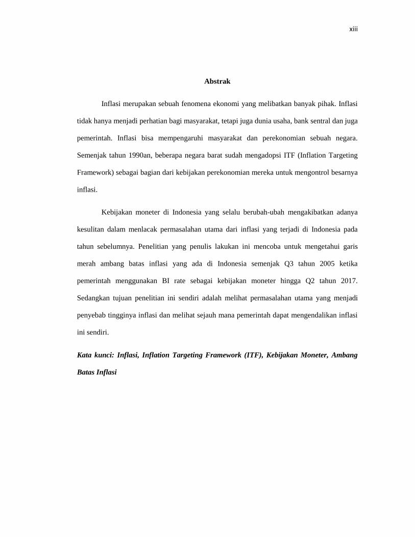
Abstrak

Inflasi merupakan sebuah fenomena ekonomi yang melibatkan banyak pihak. Inflasi

tidak hanya menjadi perhatian bagi masyarakat, tetapi juga dunia usaha, bank sentral dan juga

pemerintah. Inflasi bisa mempengaruhi masyarakat dan perekonomian sebuah negara.

Semenjak tahun 1990an, beberapa negara barat sudah mengadopsi ITF (Inflation Targeting

Framework) sebagai bagian dari kebijakan perekonomian mereka untuk mengontrol besarnya

inflasi.

Kebijakan moneter di Indonesia yang selalu berubah-ubah mengakibatkan adanya

kesulitan dalam menlacak permasalahan utama dari inflasi yang terjadi di Indonesia pada

tahun sebelumnya. Penelitian yang penulis lakukan ini mencoba untuk mengetahui garis

merah ambang batas inflasi yang ada di Indonesia semenjak Q3 tahun 2005 ketika

pemerintah menggunakan BI rate sebagai kebijakan moneter hingga Q2 tahun 2017.

Sedangkan tujuan penelitian ini sendiri adalah melihat permasalahan utama yang menjadi

penyebab tingginya inflasi dan melihat sejauh mana pemerintah dapat mengendalikan inflasi

ini sendiri.

Kata kunci: Inflasi, Inflation Targeting Framework (ITF), Kebijakan Moneter, Ambang

Batas Inflasi

1

CHAPTER I

INTRODUCTION

1.1 Background of Study

Inflation is an economic phenomenon that concerns various parties. Inflation is

not only the concern of the society, but also the concern of the business world, the central

bank, and the government. Inflation can affect the society and economy of a country. For

the society, inflation is a concern because inflation directly affects the well-being of life,

and in the business world, the rate of inflation is a very important factor in making

decisions. Inflation is also the government's concern in formulating and implementing

economic policies to improve people's welfare. Given its enormous influence on people's

lives, each country, through the monetary authority or central bank, is constantly trying to

control the inflation rate to keep it low and stable. For all countries, both developed and

developing, one of the fundamental objectives of macroeconomic policy is economic

stability.

High inflation is regarded a problem in the economy. Indonesia experienced

economic collapse for failing to control inflation volatility. Indonesia is one of the few

countries with a hyperinflationary experience. The regime of the founding President

Soekarno fell with the economy reeling when the annual inflation rate rose to 1500%

(Chowdhury & Ham, Inflation Targeting in Indonesia, 2009) The consequent untold

misery of ordinary Indonesians during 1960– 1966 created an anti-inflationary national

psyche. The New Order regime of Soeharto, thus, promulgated legislation enshrining the

“balanced budget principle” that prevented government borrowing from the central bank

(Bank Indonesia). The economic team of Soeharto was spectacularly successful in

2

preventing another episode of hyperinflation, until the Asian financial crisis of 1997–98

when inflation shot up close to 70%.

Indonesia is a country that has experienced economic collapse due to not being

able to suppress inflation rate. During the years 1958 to 1966, the Indonesian economy on

average only grew by 0.18%. At that time the average inflation reached 199%, even

touched the level of 636% in 1966. According to Subekti (2011), the main cause of the

high inflation of Indonesia in the 1960s was an unbalanced government budget and the

closest access to obtain foreign loans, so that all activities involving the government's role

must largely fund by the printing of the money. Therefore, it is not surprising that the

growth in the money supply (M1) in that era always accompanied the inflation surge with

a rapid percentage increase that is an average of 99.57%.

Indonesia's attention to inflation has been seeing as the New Order regime came

to power in 1967. The entire New Order bureaucratic cabinets share a common vision

that inflation is a major problem in the economy so control considered necessary. To

control spending, the government implements a balanced budget system. The program

proved to be quite effective. The growth in the money supply (M1) in the period 1967 to

1997 can reduce to an average of 52.7%. Nearly two decades, the economy grew about

7% with an average inflation of 12%.

Inflation control efforts continued throughout the reform period event intensified

following the 1998 monetary crisis. In 2005 Indonesia officially began implementing the

Inflation Targeting Framework, a policy aimed at achieving stability of inflation at

certain levels ranging from 4% to 10% for the short term and 3% up to 5% for the long

term (Chowdhury & Ham, Inflation Targeting in Indonesia, 2009).

3

Based on the aforementioned background, this study models the inflation in

Indonesia using the first and second-moment regression, namely conditional mean and

conditional variance, respectively. In addition to such model, this study also calculated

the threshold of deemed risky inflation, represented as conditional Value-at-Risk.

1.2 Problem Identification

The inflation-growth debate is particularly relevant for Indonesia given the

nation's historical experience. The Indonesian economy virtually came to a halt in the

1960s and the average annual inflation rate peaked at 1,500% in mid-1966. At the time,

pessimism about the prospects of the Indonesian economy was widespread. The

coincidence of extremely high rates of inflation with economic stagnation was powerful

evidence for casting inflation as 'enemy number one'. The New Order regime gave top

priority to price stability. By 1969, the annual average inflation rate was successfully

reduce to around 15% and kept under control. This provided the foundation for a period

of sustained and rapid economic growth. Following the first oil price shock, inflation rose

to 41% in 1974, but the economic management team was successful in bringing down

this figure to less than 20%.

1.3 Problem Formulation

This study focuses on two issues:

1. This study estimates inflation behavior in Indonesia using an empirical model.

The candidates for the independent variables are the interest rate, reserve

requirement, open market operation policy, base money printing, and gross

domestic product. It does not only proving theories concerning the inflation

behavior, but it also builds a good empirical model.

4

2. In addition to the built model, which is a regression model based on conditional

mean, it also models the conditional volatility or conditional variance.

Based on the built model, this study calculates the inflation threshold, which

considered dangerous to the economy.

1.4 Problem Limitation

The limitations of this study are the researcher cannot fulfill all of the resources

we demanded such as the data of Money Printing, and Obligation Price Index. The data

for Money Printing is classified and Obligation Price Index data in Indonesia was

creating since 2008.

1.5 Research Objectives

From the problem statement, the research objectives are as follows:

1. To estimate inflation behavior in Indonesia, using an empirical model.

2. Model the conditional volatility and conditional variant of inflation.

3. To calculate the inflation threshold that considered as dangerous to the economy.

1.6 Research Contributions

The research will be of benefit to the Central Bank in modeling the behaviors of

inflation. The built model can use as one of the considerations to control and combat high

inflation, which is one of the main issues in modern macro and monetary economics.

The calculated inflation threshold will be of importance in defining the dangerous

situation regarding the inflation situation. Having such threshold, the Central Bank will

5

be capable of stating whether a certain level of inflation is in need of a special

consideration and treatment.

1.7 Systematics of Writing

Chapter I: Introduction

This chapter presents Introduction, Problem Formulation, Problem Limitation,

Research Objectives, Research Contribution, and Writing Systematics.

Chapter II: Review of Related Literature

This chapter discusses concepts of inflation along with the definition, factors,

relationship between variables and references to research problem being examine. By the

end of this chapter, hypotheses analysis is present based on the literature of journal

review.

Chapter III: Research Method

This chapter describes the type and objective of this study, sample data, data

collection method, research variables, and analysis technique.

Chapter IV: Data Analysis and Discussions

This chapter discusses and analyses the data in hypotheses testing, and research

findings.

Chapter V: Conclusions and Recommendations

This chapter shows the result and presents the conclusions, research limitations, and

recommendations for institution and future researchers.

6

CHAPTER II

THEORETICAL FRAMEWORK AND LITERATURE

2.1 Theoretical Framework

Inflation knows as a major variable in macroeconomic. Inflation defined as the

increase in common price in the end. It is usually formulate as the growth in price. The

following formulae can used to calculate the inflation.

%1001

1

t

tt

tCPI

CPICPIINF

Or

%100lnln%100ln1

1

tt

t

t

t CPICPICPI

CPIINF

Both formulae represent the growth in CPI, which is consumer price index, to

measure the common price in an economy. The first formula possesses the possibility of

being non-stationarity, since it is a ratio between difference in CPI and CPI. While

difference in CPI might be stationary, the CPI itself might be non-stationary. In total, it is

possible the inflation based on this formula is non-stationary. The second formula has

greater potential to be stationary.

The study of causes of inflation has probably given rise to one of the most

significant macroeconomic debates in the field of economics. In practice; however, it is

not always easy to decompose the observed inflation into its monetary, demand-pull,

7

cost-push and structural components. The process is dynamic, and the shocks to prices

are mixed. Furthermore, inflation itself may also cause future inflation

There are two groups of economists with different views of inflation, monetarists,

and structuralizes. According to monetarists, inflation is associated with monetary

variables, the money supply is the “dominate, though not exclusive” determinant of both

the level of output and prices in the short run, and of the level of prices in the end. The

long- run level of output is not influence by the money supply, while structuralizes

suggest that inflation is the result of the unbalanced economic system, structural analysis

attempts to recognize how economic phenomena and finding the root of the permanent

disease and destruction such as inflation that evaluates lawful relationship between the

phenomena.

There are three main theories of inflation, namely cost-push inflation, demand-

pull inflation, and structural theories of inflation.

2.1.1 Cost-Push Inflation

This theory suggests that due to an increase in wages, say because of trade

unions. The rise in money wages more rapidly than the productivity of labor. The

labor unions press employers to grant wage increases considerably, thereby

raising the cost of production of commodities. Employers in turn, raise prices of

their products. Higher wages enable workers to buy as much as before in spite of

higher prices. On the other hand, the increase in prices induces unions to demand

still higher wages.

Oligopolies and monopolist firms raise the price of their products to offset the

rise in labor and cost of production to earn higher profits. There being imperfect

8

competition in the case of such firms, they are able to administered price of their

products can increase the price to any level.

A few sectors of the economy may affected by increase in money wages and

prices of their products may be rising. In many cases, their products are using as

inputs for the production of commodities in other sectors. As a result, cost of

production of other sectors will rise and thereby push up the prices of their

products. Thus, wage-push inflation in a few sectors of the economy may soon

lead to inflationary rise in prices in the entire economy. Further, an increase in

the price of imported raw materials may lead to cost-push inflation. In a way, this

increase in price is due to the increase in cost of production.

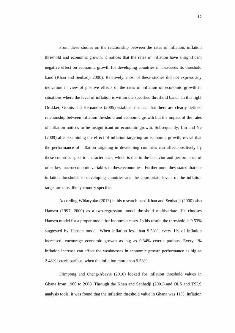
2.1.2 Demand-Pull Inflation

According to Keynes (1936) emphasized the increase in aggregate demand as the

source of demand-pull inflation. When the value of aggregate demand exceeds

the value of aggregate supply at the full employment level, the inflationary gap

arises. The larger the gap between aggregate demand and aggregate supply, the

more rapid is the inflation. The aggregate demand comprises consumption,

investment, and government expenditure. The conventional demand-pull theorists

suggest the excess of aggregate demand over aggregate supply causes inflation.

In full employment equilibrium condition, the economy reaches its maximum

production capacity. At such condition, when aggregate demand increase,

inflation takes place.

9

2.1.3 Structural Theories of Inflation

It is relate to the effect of structural factors on inflation. Structural analysis

attempts to recognize how economic phenomena and finding the root of the

permanent disease and destruction such as inflation that evaluates lawful

relationship between the phenomena. The structural theorists suggest that the

inflation is a result of structural maladjustments in the county or some of the

institutional features of business environment. In the economic structural factor

causes, supply increase related to demand-push, even if abundant unemployment

production factor is impossible or slow. Therefore, reasoning of less developed

countries, until the time not successful to change in the form of lagging behind

structure or not to make attempt for immediate self-economic growth or should

compromise with the inflation that is very severe sometimes. They have provided

two types of theories to explain the causes of inflation, namely markup theory

and bottleneck inflation theory:

a. Mark-up Theory

Prof Gardner Ackley proposed this theory. According to him, inflation is the

cumulative effect of demand-pull and cost-push activities. When aggregate

demand exceeds aggregate supply, there will be inflation, known as demand-

pull inflation. This inflation stimulates production as well as demand for

factors of production. Therefore, both the cost and price increases.

b. Bottle-Neck Inflation

Prof Otto Eckstein introduced this theory. He suggests that the main cause of

inflation is the direct relationship between wages and prices of products.

Inflation takes place when there is a simultaneous increase in wages and

prices of products. He says that the inflation occurs due to the boom in

10

capital goods and wage-price spiral. He also believes that during inflation

prices in every industry is higher, but few industries show a very high price

hike than rest of the industries. These industries are termed as bottleneck

industries, which are responsible for increase in prices of goods and services.

2.2 Literature Review

Chowdhury and Ham (2009) in his research, the empirical analysis uses the null

hypothesis of a linear vector autoregressive system of equations (VAR) against the

alternative hypothesis of a threshold vector autoregressive system of equations (TVAR)

to test whether the relationship between inflation and growth in GDP per capita shifts

when the level of inflation reaches a certain (threshold) value. Their result is the

relationship between inflation and economic growth is positive until the inflation rate

rises to a level between 8.5% and 11%. That is, inflation is likely to be harmful when it

exceeds a threshold level of around 10%.

In order to examine the issue of the existence of threshold effects in relation

between inflation and economic growth Khan and Senhadji (2000) design a new

empirical approach by using a range of econometric test. They evaluate the existence of

threshold effects and ascertain robustness by estimating the impact of sensitivity to the

estimated method, high inflation observation, the location of the threshold, date frequency

and the sensitivity to additional explanatory variables. They discovered that the pace at

which the rates of inflation significantly slow growth estimate at one to three percent for

developed countries and seven to eleven percent for developing countries. The study also

reveals some levels of negative but statistically significant relationship between the rates

of inflation and the levels of economic growth in the economies studied and the

11

associated results were robust. Although the estimated thresholds were statistically

significant at the one percent level, their stated confidence intervals were relatively wide.

This empirical concern cast some levels of doubt over the exact location of the threshold

level. Subsequently, with a ninety percent confidence interval, the researchers set an

agreed band of one to four percent for developed countries and one to twenty percent for

developing countries.

Mubarik (2005) estimated a threshold model of inflation and output growth. He

test for Granger Causality and found a unidirectional relationship between the existing

rates of inflation and the levels of economic growth. He established that the threshold

inflation was at nine percent for economic growth in Pakistan within the period of the

observation tested. To justify this result, he introduced sensitivity analysis with more

robust outcomes. The result also suggested the same level of threshold inflation for a

health domestic output level.

From a broader perspective, Kremer, Bick and Nautz (2009) in other to

expository capture the inflation threshold levels of in both developed and developing

countries, established a dynamic panel threshold model to confirm the impact of inflation

on long-run economic growth. They arrive at the view that developed economies

empirical test results confirm the fact that inflation targeting is about 2 percent. Further,

they stated that the observed level at which inflation would not affect economic growth

for developing countries is below 17 percent. Although below these thresholds, the

impact of inflation on economic growth remains insignificant. They suggested that the

empirical results did not reveal any indication of growth-enhancing effects of inflation in

developing countries.

12

From these studies on the relationship between the rates of inflation, inflation

threshold and economic growth, it notices that the rates of inflation have a significant

negative effect on economic growth for developing countries if it exceeds its threshold

band (Khan and Senhadji 2000). Relatively, most of these studies did not express any

indication in view of positive effects of the rates of inflation on economic growth in

situations where the level of inflation is within the specified threshold band. In this light

Drukker, Gomis and Hernandez (2005) establish the fact that there are clearly defined

relationship between inflation threshold and economic growth but the impact of the rates

of inflation notices to be insignificant on economic growth. Subsequently, Lin and Ye

(2009) after examining the effect of inflation targeting on economic growth, reveal that

the performance of inflation targeting in developing countries can affect positively by

these countries specific characteristics, which is due to the behavior and performance of

other key macroeconomic variables in these economies. Furthermore, they stated that the

inflation thresholds in developing countries and the appropriate levels of the inflation

target are most likely country specific.

According Widaryoko (2013) in his research used Khan and Senhadji (2000) also

Hansen (1997, 2000) as a two-regression model threshold multivariate. He chooses

Hansen model for a proper model for Indonesia cases. In his result, the threshold is 9.53%

suggested by Hansen model. When inflation less than 9.53%, every 1% of inflation

increased, encourage economic growth as big as 0.34% ceteris paribus. Every 1%

inflation increase can affect the weaknesses in economic growth performance as big as

2.48% ceteris paribus, when the inflation more than 9.53%.

Frimpong and Oteng-Abayie (2010) looked for inflation threshold values in

Ghana from 1960 to 2008. Through the Khan and Senhadji (2001) and OLS and TSLS

analysis tools, it was found that the inflation threshold value in Ghana was 11%. Inflation

13

has a positive effect on economic growth when the value is below 11% and will have a

negative impact if the value exceeds 11%. Variables used to consist of inflation,

economic growth of investment growth, the growth of money supply, the growth of the

labor force, and terms of trade growth.

First research that stated there is a non-linear relationship between inflation and

economic growth are Fischer (1993) and Sarel (1996). They found structural break point.

After that, other researchers start to explore this study with estimate the value of the

structural break point. The term structural break point knows as inflation threshold. The

study, among others Khan and Senhadji (2001) found threshold inflation for developed

country is 1-2% and developing country is 11-12%. Espinoza, Prasad, Leon (2010) found

for all group country (except for advance countries) is 10%. Kremer, Bick, and Nautz

(2013) found 2% for industrialize countries and 17% for non-industrialize countries.

Vinayagathasan (2013) found 5.43% for 32 Asian countries. Baglan and Yoldasz (2014)

found 12% threshold inflation for developing countries. Then, Ayyoub (2016) found

13.48%, 14.48%, 15.37%, and 40% for aggregate GDP, industrial, services and

agriculture sectors respectively.

The study included Indonesia as an observation by Khan and Senhadji (2001),

Espinoza, Prasad, and Leon (2010) found that as a developing country, Indonesia has a

level of threshold inflation above 10%. Baglan, and Yoldasz (2014) found 12% threshold

inflation for developing countries. In that study, the hypothesis is non-linear relationship

between inflation and economic growth in Indonesia. From these study, Khan and

Senhadji (2001), Espinoza, Prasad, and Leon (2010), Baglan and Yoldasz (2014), they

found that as developing country Indonesia have threshold inflation above 10%, but

Thanh (2015) found threshold level for developing countries in Asia region lower than

those for other developing countries. Thanh (2015) stated threshold inflation for ASEAN-

14

5 (include Indonesia) is 7.84%. Vinayagathasan (2013) also found threshold inflation for

Asian countries is 5.43% where Indonesia includes as observation. From these study is

suspected Indonesia level threshold inflation may be lower again with current economic

condition tend to be stable and low inflation policy.

Furthermore, four studies examine relationship between inflation and economic

growth in Indonesia. Chowdhury and Siregar (2004) using the quadratic equation and

find the threshold value of inflation in Indonesia at 20.50%. The interpretation is inflation

positive effect on economic growth when its value is below 20% and will have a negative

impact if the value exceeds 20%. While the results of the estimation using threshold

vector auto-regression (TVAR) conducted by Chowdhury and Ham (2009) concluded

threshold inflation in Indonesia is between on 8.50 to 11%. Widaryoko (2013) using a

model of Hansen in 2000 found that inflation threshold in Indonesia at 9.53%. Winarno

(2014) uses a dynamic panel threshold models found inflation threshold value exists for

Indonesia and the estimated threshold regression model shows the threshold value is

4.62%. Different level threshold inflation may have caused by the range data observed,

because in 1970-1997 Indonesia was not applied low inflation policies and after 1999,

Indonesia started using low inflation policy.

The Opinions by Sepehri and Moshiri (2004), Kremer, Bick and Nautz (2013)

stated that the study of inflation and economic growth should be the focus in the country,

because the economic structure of each country is different. In addition, there are studies

examining the same country but get different results for different period. That is likely

due to economic structure of the country has changed over time. Therefore, this paper

will use different method and up-to-date data for estimate threshold inflation in Indonesia

in newest condition.

15

A natural starting point for the empirical analysis of inflation thresholds is the

panel threshold model introduced by Hansen (1999) which is design to estimate threshold

values instead of imposing them. Yet, the application of Hansen’s threshold model to the

empirical analysis of the inflation–growth nexus is not without problems. The most

important limitation of Hansen’s model is that all repressors are required to be

exogenous. In growth regressions with panel data, the exogeneity assumption is

particularly severe, because initial income as a crucial variable is endogenous by

construction. Caselli et al. (1996) already demonstrated for linear panel models of

economic growth that the endogeneity bias could be substantial. So far, dynamic versions

of Hansen’s panel threshold model have not been available.

Munir and Mansur (2009) found that inflation threshold value in Malaysia during

1970 to 2005 was 3.89%. The method used is conditional least squares with the

variability of inflation, economic growth, Money supply growth (M2), the growth of

PMTB, FDI, and growth export.

Different from existing research, our research use monetary transmission policy

instrument such as; Reserve Requirements, Money Supply, Bank Indonesia Certificate,

and Overnight Bank Rates. In addition, Exchange Rate as represent outside factor may

influence inflation.

2.3 Hypothesis

There is an influence from Reserve Requirements, Money Supply, Bank

Indonesia Certificate, Rates and Exchange Rate to Inflation in Indonesia. The rising oil

price can give highest pressure to inflation in Indonesia and the average value at risk of

inflation threshold in Indonesia not more than 10%.

16

Chapter III

METHODS

From the above discussion, this study models inflation uses some independent

variables namely; interest rate, reserve requirement, open market operation policy, base

money printing, and gross domestic product.

To avoid estimating a spurious regression, this study will conduct unit root tests

to test the presence of non-stationary variables. Based on the status of the stationarity

levels, this study takes into considerations two model candidates, namely short run, and

long run models. The chosen model could be the combination of both, generally known

as an Error Correction Model (ECM). This ECM can be built from two different

situations, namely all variables are of I(1), namely integrated into the first difference, or

the variables are the combination of both I (1) and I (0), where I (0) states that the

variables are stationary in level.

If all of the variables are of I (1), a co-integration based on Engle-Granger test

will be conducted. If the variables are the combination of I (1) and I (0), an ARDL

(Autoregressive Distributed Lag) model will be estimated, which will be followed by a

bounds test to test for the presence of co-integration.

As discussed, this study models the inflation using both conditional mean and

conditional variance. The conditional variance is then employee to calculate the VaR.

Different from non-conditional VaR, where the value is calculate as the mean plus or

minus the distribution value times the standard deviation, this study uses conditional VaR

since the standard deviation (volatility) is a conditional volatility, modeled by a family of

GARCH model. Some possible second-moment models to estimate are ARCH, GARCH,

17

GJR, and EGARCH models. The ARCH, GARCH, GJR, and EGARCH models create by

Engle (1982), Bollerslev (1986), Glosten, Jagannathan and Runkle (1993), and Nelson

(1991), respectively.

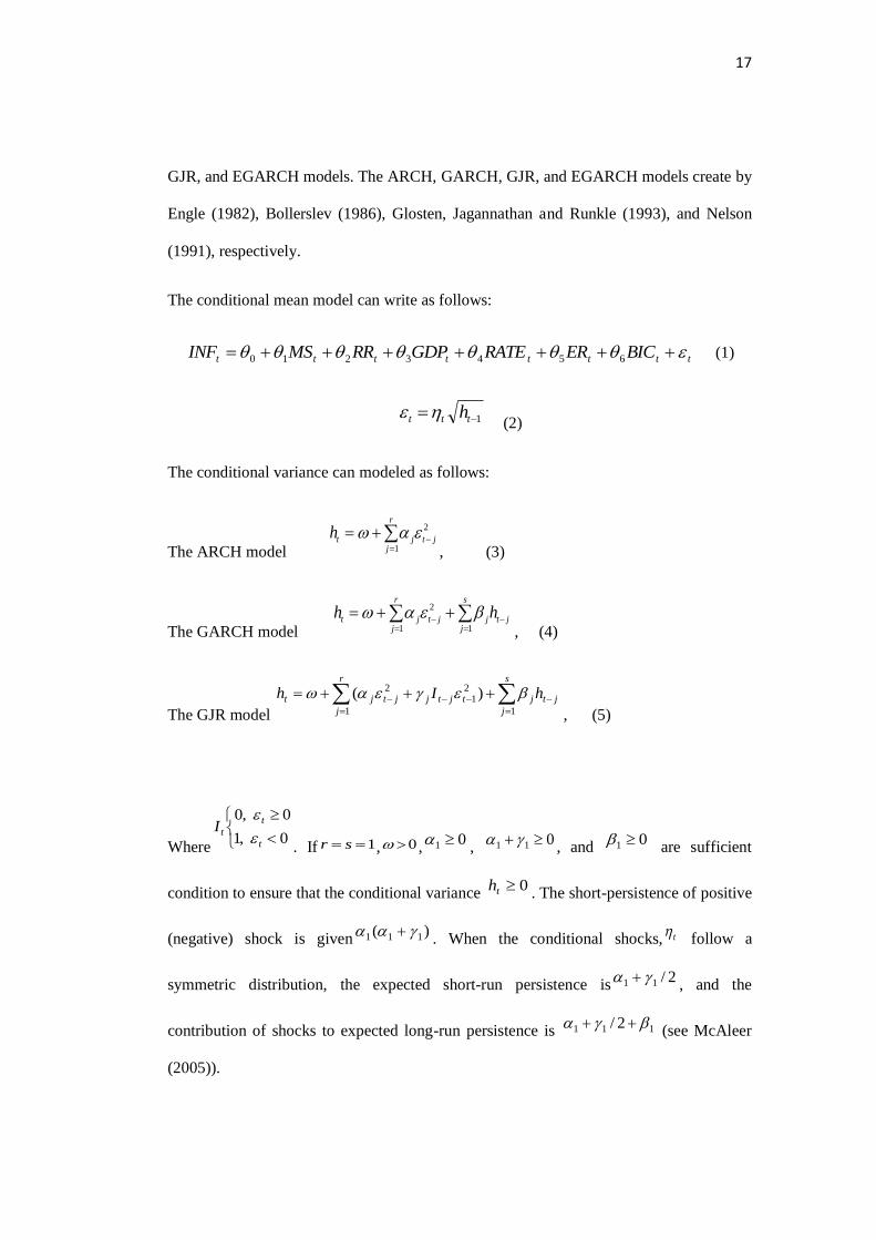
The conditional mean model can write as follows:

tttttttt BICERRATEGDPRRMSINF 6543210 (1)

1 ttt h (2)

The conditional variance can modeled as follows:

The ARCH model

2

1jt

r

jjt

h

, (3)

The GARCH model

s

jjtjjt

r

jjt

hh1

2

1

, (4)

The GJR model

s

j

jtjtjtjjt

r

j

jt hIh1

21

2

1

)(

, (5)

Where

0,1

0,0

t

t

tI

. If 1 sr , 0 ,01

, 011

, and 01

are sufficient

condition to ensure that the conditional variance 0th

. The short-persistence of positive

(negative) shock is given)( 111

. When the conditional shocks, t follow a

symmetric distribution, the expected short-run persistence is2/11

, and the

contribution of shocks to expected long-run persistence is 111 2/ (see McAleer

(2005)).

18

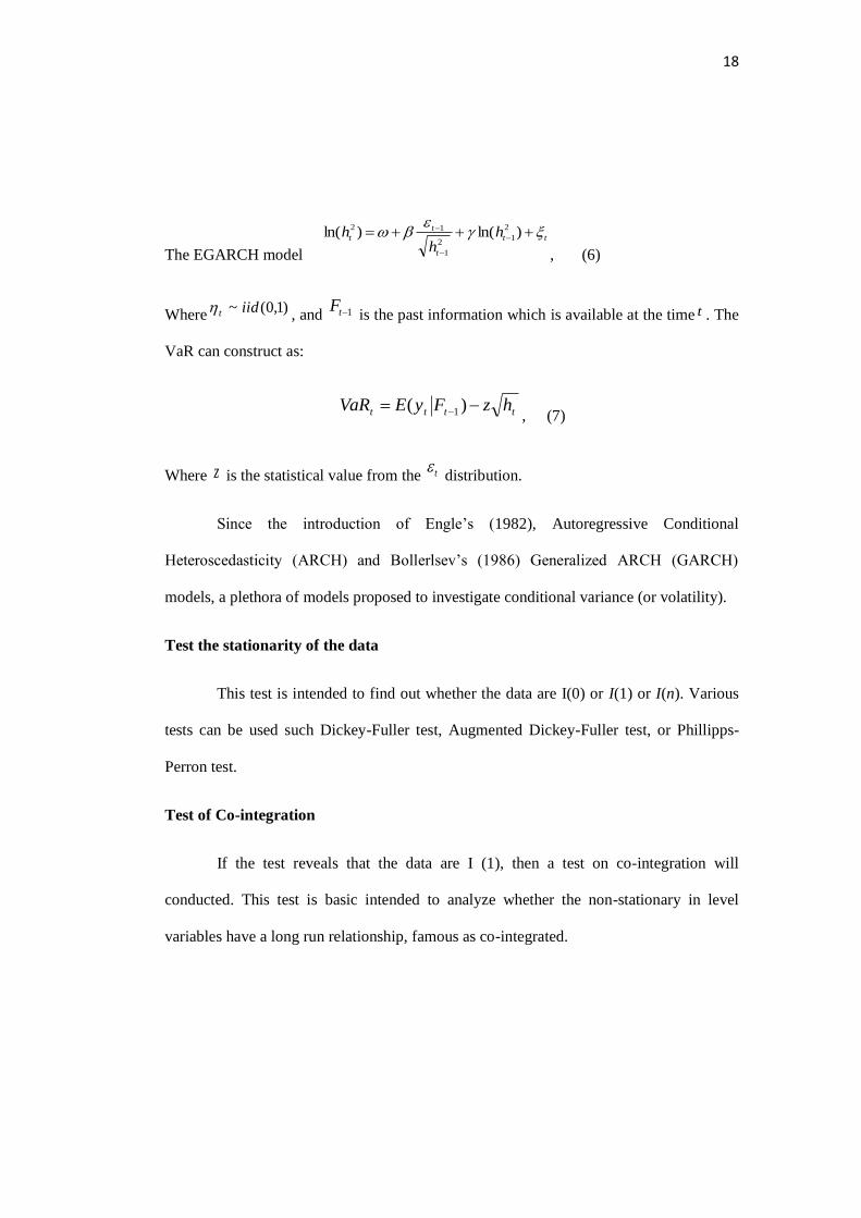
The EGARCH model

tt

t

t

t hh

h

)ln()ln( 2

12

1

12

, (6)

Where)1,0(~ iidt , and 1tF

is the past information which is available at the time t . The

VaR can construct as:

tttt hzFyEVaR )( 1 , (7)

Where z is the statistical value from the t distribution.

Since the introduction of Engle’s (1982), Autoregressive Conditional

Heteroscedasticity (ARCH) and Bollerlsev’s (1986) Generalized ARCH (GARCH)

models, a plethora of models proposed to investigate conditional variance (or volatility).

Test the stationarity of the data

This test is intended to find out whether the data are I(0) or I(1) or I(n). Various

tests can be used such Dickey-Fuller test, Augmented Dickey-Fuller test, or Phillipps-

Perron test.

Test of Co-integration

If the test reveals that the data are I (1), then a test on co-integration will

conducted. This test is basic intended to analyze whether the non-stationary in level

variables have a long run relationship, famous as co-integrated.

19

ECM Estimation

If the co-integration does exist, then following the Granger Theorem, we will

build an Error Correction Model to tie the short-run equilibrium on the relationship

between variables, and the long run situation, reflected in the regression model in level.

3.1 Variable of Research and Definition of Variable Operations

3.1.1 Variable of Research

The dependent variable of this study, namely the focus of the research, is the

inflation of Indonesia. The independent variables include interest rate, reserve

requirement, open market operation policy, base money printing, and gross domestic

product.

3.1.2 Definition of Variable Operation

Interbank Overnight (O/N) Rates (Interest rate)

To achieve the overriding monetary policy objective, Bank Indonesia has

implemented a monetary policy framework for management of interest rates (interest rate

target). The policy rate, commonly known as the BI 7DDR, adopted in the Board of

Governors Meeting at Bank Indonesia. At the operational level, the BI 7DDR reflected in

movement in the Interbank Overnight (O/N) Rate.

The interbank money market is the activity of lending and borrowing money

between one bank and another bank. An interbank rate represents the price formed in a

deal between parties lending and borrowing funds. Activity on the interbank conducted

over the counter (OTC) through deals between borrowers and holders of funds arranged

without passing through an exchange floor. Interbank tenors range from one working day

(overnight) to one year.

20

The interest rate is a strong candidate that might influence inflation. The theory

said that as interest rate increases, people save their money into banks and delay

consumption spending. This will reduce the money supply, and decreases inflation.

Statutory Reserve Requirement (Giro Wajib Minimum, GWM)

In Indonesia called as Giro Wajib Minimum (GWM), is the minimum amount

required to maintain by a bank, the amount of which determined by Bank Indonesia at a

certain percentage of third party funds. Since 24 October 2008, statutory reserve

requirement in Indonesia has two type of statutory reserve requirement: GWM primary

and secondary GWM. The primary GWM shall be the minimum deposit required by the

bank in the form of a demand deposit account balance at Bank Indonesia. The amount of

which determined by Bank Indonesia at a certain percentage of third party funds, and the

secondary GWM shall be the minimum reserves required to be maintained by banks in

the form of Bank Indonesia Certificates, Government Bonds and / or Excess Reserve, at a

rate determined by Bank Indonesia at a certain percentage of third party funds.

The reserve requirement is another strong candidate that might influence

inflation. The theory said that as the central bank increases reserve requirement, common

banks have less money to be lent, that will eventually reduce the money supply, and

decreases inflation.

Bank Indonesia Certificates (Open Market Operation)

Securities denominated in Rupiah currency issued by Bank Indonesia in

recognition of short-term debt. In this study, use daily, average number of sales of Bank

Indonesia Certificate published by Bank Indonesia.

The open market operation is a policy held by the Central Bank to control

inflation. It works by selling and buying government or central bank’s bonds. If the

21

central bank wishes to reduce inflation, it can sell its bonds to the people. As the people

buy the central bank bonds, their money flows from the circulation into the central bank,

and it will reduce the money supply, and reduce inflation.

Gross Domestic Product

One of the important indicators to oversight economic condition in a country

during certain period time, whether based on actual price or constant price, in this study

use current prices GDP based on current price displays the additional values of goods and

services calculated using the price in the current year. GDP based on current price

displays the additional values of goods and services calculated using the price in the

current year. Currently, GDP data published by Statistics Indonesia calculated using

production approach and expenditure approach.

Different from the other candidate of independent variables in this study, which

influence money supply to influence inflation, GDP influences the money demand in its

way to influence inflation. As GDP increases, the need for liquidity increases. This will

increase money demand and increases inflation.

Data

All the data are secondary data in nature. The researcher wishes to be able to find

the data from various sources, namely from Badan Pusat Statistik, Bank Indonesia,

Ministry of Finance, and some other possible sources.

22

CHAPTER IV

RESULT AND DATA ANALYSIS

Selected Model: ARDL(5, 5, 5, 5, 5, 5, 5)

Variable Coefficient Std. Error t-Statistic Prob.*

INFLATION(-1) 5.563135 0.073993 75.18457 0.0085

INFLATION(-2) -0.238816 0.034057 -7.012162 0.0902

INFLATION(-3) -1.976820 0.045662 -43.29212 0.0147

INFLATION(-4) 8.554466 0.123317 69.36999 0.0092

INFLATION(-5) -6.316263 0.087766 -71.96697 0.0088

M2 0.002216 3.16E-05 70.23656 0.0091

M2(-1) -0.004369 6.11E-05 -71.48273 0.0089

M2(-2) -0.002753 4.42E-05 -62.32189 0.0102

M2(-3) -0.000778 1.79E-05 -43.55969 0.0146

M2(-4) 0.002530 3.64E-05 69.56267 0.0092

M2(-5) 0.003392 4.92E-05 68.94108 0.0092

GWM1 -13.26170 0.212070 -62.53450 0.0102

GWM1(-1) -1.808876 0.049810 -36.31519 0.0175

GWM1(-2) 22.00652 0.261915 84.02160 0.0076

GWM1(-3) 9.902550 0.138793 71.34785 0.0089

GWM1(-4) 2.691718 0.056552 47.59729 0.0134

GWM1(-5) 3.170784 0.061690 51.39834 0.0124

GDP -0.003650 4.87E-05 -74.97728 0.0085

GDP(-1) -0.000799 1.91E-05 -41.81386 0.0152

GDP(-2) -0.000597 1.22E-05 -49.15216 0.0130

GDP(-3) 0.002701 4.28E-05 63.14761 0.0101

GDP(-4) 0.005173 8.03E-05 64.42936 0.0099

GDP(-5) -0.004155 4.86E-05 -85.47957 0.0074

RATE2 -14.11192 0.195031 -72.35727 0.0088

RATE2(-1) 6.621513 0.164107 40.34865 0.0158

RATE2(-2) -44.66601 0.588847 -75.85334 0.0084

RATE2(-3) -16.39659 0.256499 -63.92458 0.0100

RATE2(-4) -5.838201 0.098801 -59.09028 0.0108

RATE2(-5) 13.05059 0.192763 67.70270 0.0094

ER 0.000335 4.74E-06 70.62999 0.0090

ER(-1) 0.000115 1.83E-06 62.61399 0.0102

ER(-2) 0.000392 5.72E-06 68.61645 0.0093

ER(-3) -0.000217 2.97E-06 -73.17003 0.0087

ER(-4) 2.36E-05 4.56E-07 51.81984 0.0123

ER(-5) -3.89E-05 1.20E-06 -32.35473 0.0197

SBI 0.002045 2.97E-05 68.75427 0.0093

SBI(-1) -0.001708 2.20E-05 -77.63315 0.0082

SBI(-2) 0.006065 7.91E-05 76.70830 0.0083

SBI(-3) 0.001552 2.45E-05 63.38129 0.0100

SBI(-4) 0.001915 2.89E-05 66.26629 0.0096

Dependent Variable: INFLATION

Method: ARDL

23

SBI(-5) 0.000809 1.23E-05 65.70911 0.0097

C -2.292454 0.033468 -68.49659 0.0093

Table 4.1: ARDL

4.1 ARDL

From 43 observation after adjustment, 42 data have probability value below 0.05

of standards error, is mean 42 data have significant result to influence inflation, only

variable inflation in lag two not significant because have probability value above 0.05 of

standard error, 0.0902 . The data processed use Hannan-Quinn criterion (HQ) model

selection method; the data have automatic selection to looking for best result. The data

processed five of maximum dependent lags and five of dynamic regression, automated

selection. The Selected model select by ARDL are in lag five.

The dependent variable Inflation, in lag five has probability value 0.0088; does

statistically significant to influence inflation with coefficient level -6.316263, mean

previous inflation negatively influence current inflation by 6.3%, strengthen the result

that found by Larasati & Amri (2017). This indicate inflation in Indonesia well controlled

and managed by Bank Indonesia as central bank to maintain inflation keep on track by

implementing a policy mix with an enhanced inflation-targeting framework.

Independent variable M2, in lag five has probability value 0.0092, does

statistically significant to influence inflation with coefficient value 0.003392, mean

Money Supply (M2) positively give influence to inflation by 0.003%. The finding is in

line with Sutawijaya (2012),Nguyen (2015), and Langi, Masinambow, & Siwu (2014),

they found that the money supply has a positive and significant effect on inflation.

Independent variable GWM, Statutory Reserve Requirements, in lag five has

probability value 0.0124, does statistically significant to influence inflation with

24

coefficient value 3.170784, mean GWM positively give influence to inflation by 3.17%.

This finding is not in line with Setyawan (2010), his found GWM negatively influence

inflation.

Independent variable GDP, Gross Domestic Product, in lag five has probability

value 0.0074, does statistically significant to influence inflation with coefficient value -

0.004155, mean GDP negatively influence inflation by 0.004%. Negative relationship

between GDP as economic growth indicator and inflation is important, as it quite often

occurs in practice, as ascertained by empirical literature.

Independent variable Interest Rate in lag five has probability value 0.0094, does

statistically significant to influence inflation with coefficient value 13.05059, mean

Interest Rate influence inflation by 13.05%. Independent variable ER, exchange rate, in

lag five has probability value 0.0197, does statistically significant to influence inflation

with coefficient value -3.89E-05, mean exchange rate negatively influence inflation by

3.89%. Variable SBI, Bank Indonesia’s Certificate, in lag five have probability value

0.0097, does statistically significant to influence inflation with coefficient value

0.000809, mean.

4.2 Bound Test

F-Bounds Test

Null Hypothesis: No levels

relationship

Test Statistic Value Signif. I(0) I(1)

Asymptotic:

n=1000

F-statistic 2680.786 10% 1.99 2.94

K 6 5% 2.27 3.28

2.5% 2.55 3.61

1% 2.88 3.99

Table 4.2: Bound Test

25

The value of F-statistic is 2680.7866, is greater than any value of bound at any

significant level, mean the data have long-run relationship between the variables.

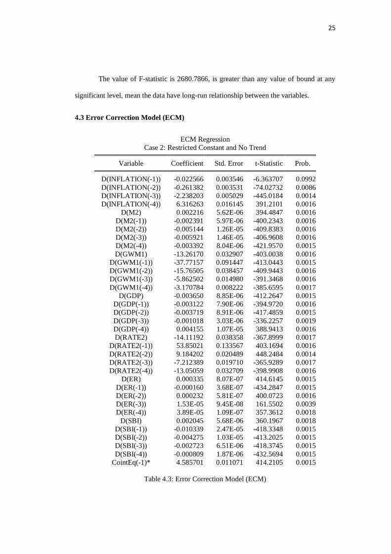
4.3 Error Correction Model (ECM)

ECM Regression

Case 2: Restricted Constant and No Trend

Variable Coefficient Std. Error t-Statistic Prob.

D(INFLATION(-1)) -0.022566 0.003546 -6.363707 0.0992

D(INFLATION(-2)) -0.261382 0.003531 -74.02732 0.0086

D(INFLATION(-3)) -2.238203 0.005029 -445.0184 0.0014

D(INFLATION(-4)) 6.316263 0.016145 391.2101 0.0016

D(M2) 0.002216 5.62E-06 394.4847 0.0016

D(M2(-1)) -0.002391 5.97E-06 -400.2343 0.0016

D(M2(-2)) -0.005144 1.26E-05 -409.8383 0.0016

D(M2(-3)) -0.005921 1.46E-05 -406.9608 0.0016

D(M2(-4)) -0.003392 8.04E-06 -421.9570 0.0015

D(GWM1) -13.26170 0.032907 -403.0038 0.0016

D(GWM1(-1)) -37.77157 0.091447 -413.0443 0.0015

D(GWM1(-2)) -15.76505 0.038457 -409.9443 0.0016

D(GWM1(-3)) -5.862502 0.014980 -391.3468 0.0016

D(GWM1(-4)) -3.170784 0.008222 -385.6595 0.0017

D(GDP) -0.003650 8.85E-06 -412.2647 0.0015

D(GDP(-1)) -0.003122 7.90E-06 -394.9720 0.0016

D(GDP(-2)) -0.003719 8.91E-06 -417.4859 0.0015

D(GDP(-3)) -0.001018 3.03E-06 -336.2257 0.0019

D(GDP(-4)) 0.004155 1.07E-05 388.9413 0.0016

D(RATE2) -14.11192 0.038358 -367.8999 0.0017

D(RATE2(-1)) 53.85021 0.133567 403.1694 0.0016

D(RATE2(-2)) 9.184202 0.020489 448.2484 0.0014

D(RATE2(-3)) -7.212389 0.019710 -365.9289 0.0017

D(RATE2(-4)) -13.05059 0.032709 -398.9908 0.0016

D(ER) 0.000335 8.07E-07 414.6145 0.0015

D(ER(-1)) -0.000160 3.68E-07 -434.2847 0.0015

D(ER(-2)) 0.000232 5.81E-07 400.0723 0.0016

D(ER(-3)) 1.53E-05 9.45E-08 161.5502 0.0039

D(ER(-4)) 3.89E-05 1.09E-07 357.3612 0.0018

D(SBI) 0.002045 5.68E-06 360.1967 0.0018

D(SBI(-1)) -0.010339 2.47E-05 -418.3348 0.0015

D(SBI(-2)) -0.004275 1.03E-05 -413.2025 0.0015

D(SBI(-3)) -0.002723 6.51E-06 -418.3745 0.0015

D(SBI(-4)) -0.000809 1.87E-06 -432.5694 0.0015

CointEq(-1)* 4.585701 0.011071 414.2105 0.0015

Table 4.3: Error Correction Model (ECM)

26

Interestingly in Error Correction Term show the model have positive coefficient

(4.585701) and have significant result (0.0015), the model does not have co-integration in

long run. In Durbin-Watson stat result 3.497113 is greater than two but less than four,

mean the model have negative autocorrelation.

4.4 Value at Risk of Inflation Threshold

Graphic 4.4: VaR

0

0.05

0.1

0.15

0.2

0.25

20

05Q

3

20

06Q

1

20

06Q

3

20

07Q

1

20

07Q

3

20

08Q

1

20

08Q

3

20

09Q

1

20

09Q

3

20

10Q

1

20

10Q

3

20

11Q

1

20

11Q

3

20

12Q

1

20

12Q

3

20

13Q

1

20

13Q

3

20

14Q

1

20

14Q

3

20

15Q

1

20

15Q

3

20

16Q

1

20

16Q

3

20

17Q

1

VaR

Actual VaR_t_10% VaR_z_10%

VaR_t_5% VaR_z_5%

27

Graphic 4.5: VaR_t_10%

Graphic 4.6: VaR_z_10%

0

0.05

0.1

0.15

0.2

0.25

2005

Q3

2006

Q2

2007

Q1

2007

Q4

2008

Q3

2009

Q2

2010

Q1

2010

Q4

2011

Q3

2012

Q2

2013

Q1

2013

Q4

2014

Q3

2015

Q2

2016

Q1

2016

Q4

VaR_t_10%

Actual VaR_t_10%

0

0.05

0.1

0.15

0.2

0.25

2005

Q3

2006

Q2

2007

Q1

2007

Q4

2008

Q3

2009

Q2

2010

Q1

2010

Q4

2011

Q3

2012

Q2

2013

Q1

2013

Q4

2014

Q3

2015

Q2

2016

Q1

2016

Q4

VaR_z_10%

Actual VaR_z_10%

28

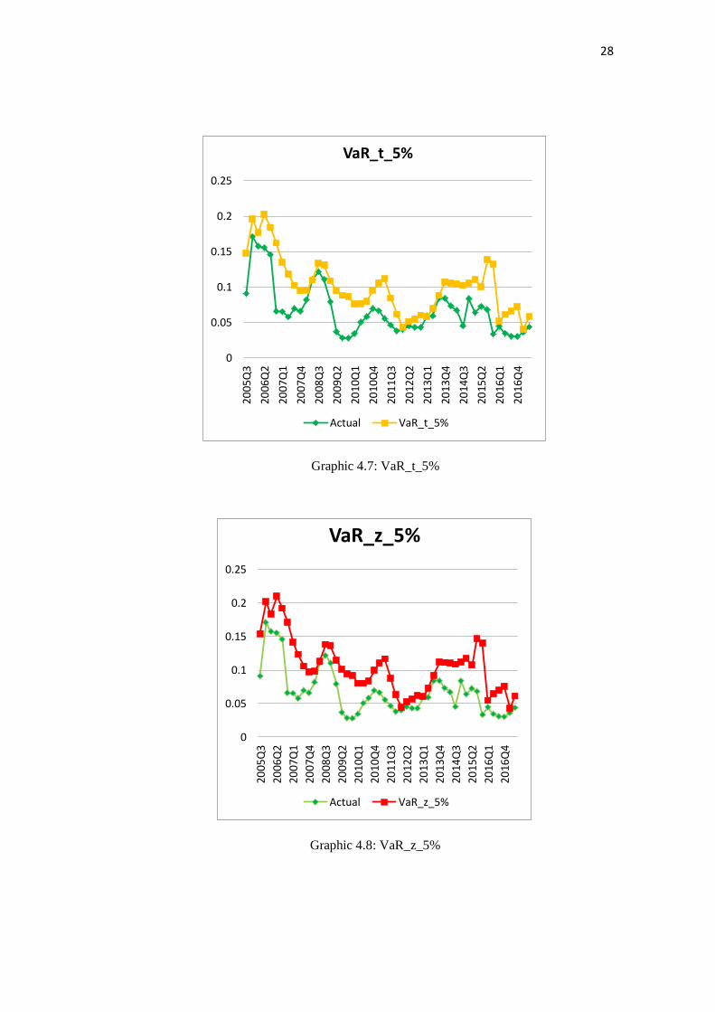
Graphic 4.7: VaR_t_5%

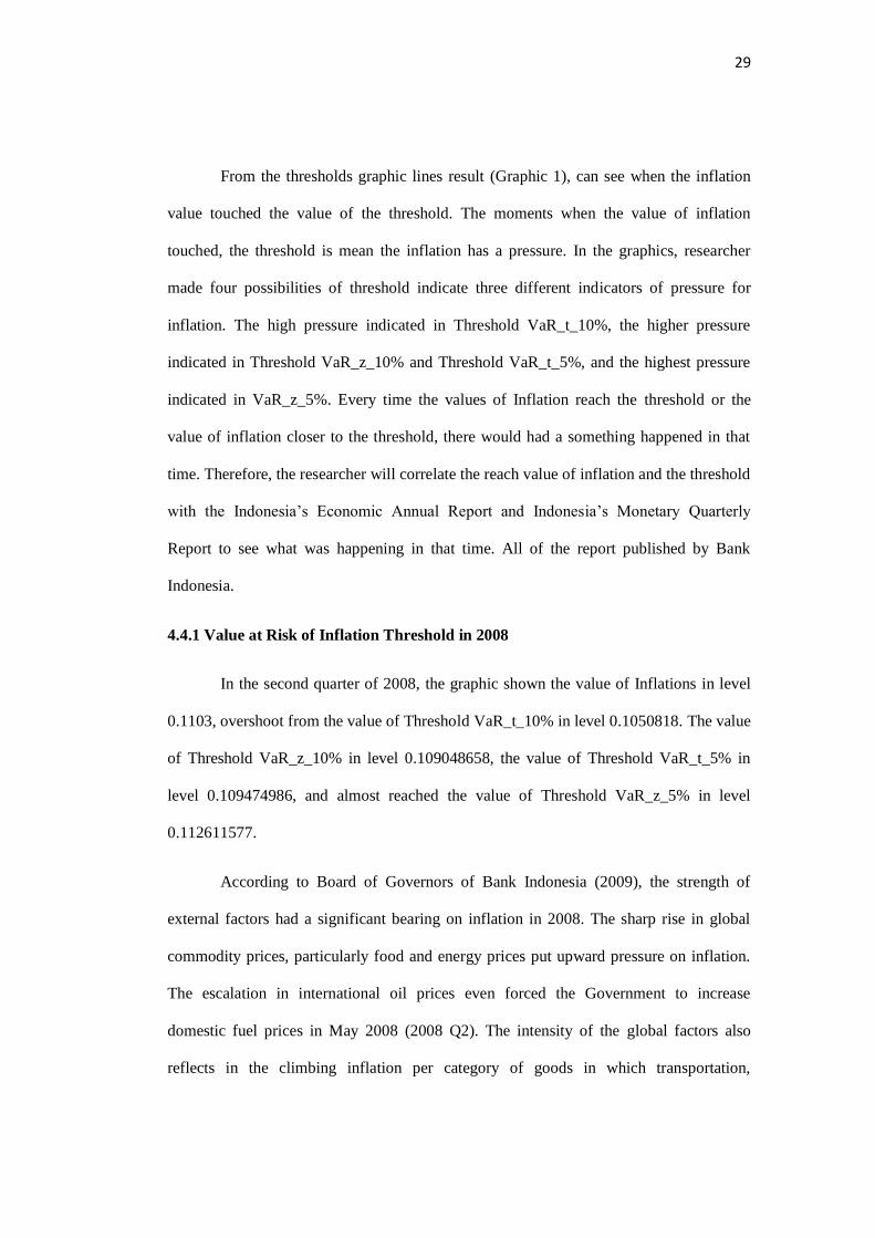
Graphic 4.8: VaR_z_5%

0

0.05

0.1

0.15

0.2

0.25

2005

Q3

2006

Q2

2007

Q1

2007

Q4

2008

Q3

2009

Q2

2010

Q1

2010

Q4

2011

Q3

2012

Q2

2013

Q1

2013

Q4

2014

Q3

2015

Q2

2016

Q1

2016

Q4

VaR_t_5%

Actual VaR_t_5%

0

0.05

0.1

0.15

0.2

0.25

2005

Q3

2006

Q2

2007

Q1

2007

Q4

2008

Q3

2009

Q2

2010

Q1

2010

Q4

2011

Q3

2012

Q2

2013

Q1

2013

Q4

2014

Q3

2015

Q2

2016

Q1

2016

Q4

VaR_z_5%

Actual VaR_z_5%

29

From the thresholds graphic lines result (Graphic 1), can see when the inflation

value touched the value of the threshold. The moments when the value of inflation

touched, the threshold is mean the inflation has a pressure. In the graphics, researcher

made four possibilities of threshold indicate three different indicators of pressure for

inflation. The high pressure indicated in Threshold VaR_t_10%, the higher pressure

indicated in Threshold VaR_z_10% and Threshold VaR_t_5%, and the highest pressure

indicated in VaR_z_5%. Every time the values of Inflation reach the threshold or the

value of inflation closer to the threshold, there would had a something happened in that

time. Therefore, the researcher will correlate the reach value of inflation and the threshold

with the Indonesia’s Economic Annual Report and Indonesia’s Monetary Quarterly

Report to see what was happening in that time. All of the report published by Bank

Indonesia.

4.4.1 Value at Risk of Inflation Threshold in 2008

In the second quarter of 2008, the graphic shown the value of Inflations in level

0.1103, overshoot from the value of Threshold VaR_t_10% in level 0.1050818. The value

of Threshold VaR_z_10% in level 0.109048658, the value of Threshold VaR_t_5% in

level 0.109474986, and almost reached the value of Threshold VaR_z_5% in level

0.112611577.

According to Board of Governors of Bank Indonesia (2009), the strength of

external factors had a significant bearing on inflation in 2008. The sharp rise in global

commodity prices, particularly food and energy prices put upward pressure on inflation.

The escalation in international oil prices even forced the Government to increase

domestic fuel prices in May 2008 (2008 Q2). The intensity of the global factors also

reflects in the climbing inflation per category of goods in which transportation,

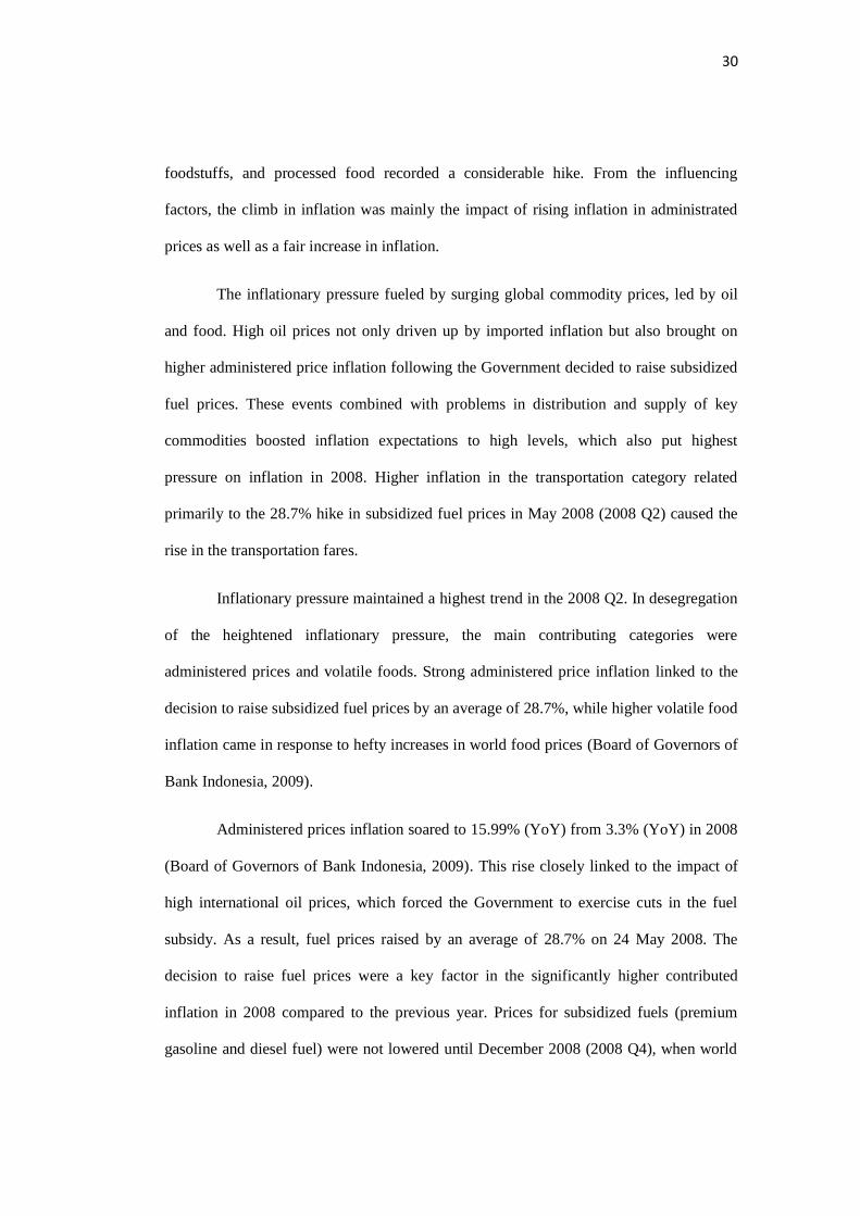
30

foodstuffs, and processed food recorded a considerable hike. From the influencing

factors, the climb in inflation was mainly the impact of rising inflation in administrated

prices as well as a fair increase in inflation.

The inflationary pressure fueled by surging global commodity prices, led by oil

and food. High oil prices not only driven up by imported inflation but also brought on

higher administered price inflation following the Government decided to raise subsidized

fuel prices. These events combined with problems in distribution and supply of key

commodities boosted inflation expectations to high levels, which also put highest

pressure on inflation in 2008. Higher inflation in the transportation category related

primarily to the 28.7% hike in subsidized fuel prices in May 2008 (2008 Q2) caused the

rise in the transportation fares.

Inflationary pressure maintained a highest trend in the 2008 Q2. In desegregation

of the heightened inflationary pressure, the main contributing categories were

administered prices and volatile foods. Strong administered price inflation linked to the

decision to raise subsidized fuel prices by an average of 28.7%, while higher volatile food

inflation came in response to hefty increases in world food prices (Board of Governors of

Bank Indonesia, 2009).

Administered prices inflation soared to 15.99% (YoY) from 3.3% (YoY) in 2008

(Board of Governors of Bank Indonesia, 2009). This rise closely linked to the impact of

high international oil prices, which forced the Government to exercise cuts in the fuel

subsidy. As a result, fuel prices raised by an average of 28.7% on 24 May 2008. The

decision to raise fuel prices were a key factor in the significantly higher contributed

inflation in 2008 compared to the previous year. Prices for subsidized fuels (premium

gasoline and diesel fuel) were not lowered until December 2008 (2008 Q4), when world

31

oil prices resumed the decline. This price cut had the first-round effect on inflation of -

0.54% (Board of Governors of Bank Indonesia, 2009).

Nevertheless, inflationary pressures eased quite significantly in 2008 Q4 as the

global commodity prices fell and the slowdown of the world economy deepened. Aside

from that, the Government policy to lower domestic fuel prices in December 2008 (2008

Q4) in line with the declining world oil prices alleviated further the inflationary pressure.

The graphic shows the value of threshold stay away from the value of inflation.

The less inflationary pressure came mainly in response to falling international

commodity prices followed by a comparatively limited easing of domestic commodity

prices and the price cuts for premium gasoline and automotive diesel in December 2008

(2008 Q4). Analyzed by influencing factors, mounting inflation in 2008 was explains

mainly by heightened inflation in administered prices. Government decisions concerning

administered prices, most importantly to raise subsidized fuel prices on 24 May 2008

combined with escalating global foodstuff prices were responsible for escalating

inflationary pressure, but subsequently weakened during 2008 Q4.

4.4.2 Value at Risk of Inflation Threshold in 2009

Interestingly, Inflationary pressure in 2009 was generally minimal. The graphics

show declining inflation trend and along with the value of inflation stay away from the

value of threshold is mean inflation had less pressure. Inflation plunged to 2.78% from

11.06% in 2008. Inflation in 2009 also came below the 2009 inflation target set at 4.5% ±

1% (Board of Governors of Bank Indonesia, 2010).

According to Board of Governors of Bank Indonesia (2010), the minimal

inflation in 2009 explain largely by Bank Indonesia policies in restoring market

confidence that subsequently paved the way for appreciation in the rupiah. This, in turn,

32

helped to shape improved inflation expectations. The milder inflation expectations were

also explain largely by lower administered prices and volatile foods inflation.

Administered prices inflation fell below the trend because of the positive influence of the

Government decision to lower subsidized fuel prices in early 2009. At the same time,

modest volatile foods inflation below the trend owes much, to successful government

measures in securing the supply and distribution of vital food staples and energy. The low

inflation in 2009 resulted from the decline across all inflation components and categories

of goods. The reduced inflation linked primarily to the effect of the cut in subsidized fuel

prices. Even in 2009, the trends of inflation is decline is in line with the slower economic

activity and effected on slowing economic growth because of slowing Indonesia’s export

performance and domestic consumption.

4.4.3 Value at Risk of Inflation Threshold in 2012

In the first quarter of 2012, the value of inflation is in level 0.0397; nearly reach

the value of Threshold VaR_t_10% in level 0.0416411. According to Board of Governors

of Bank Indonesia (2013), in 2012 Q1 inflation expectations have increased due to the

expected changes in policies related to subsidized fuel. At that time, government had a

plan to increased subsidize fuel, was rejected by parliament. The uncertainty decision

from government for increased subsidize fuel, effected to the people to creating

expectation and resulted almost high-pressure inflation because of expectations inflation

among the people.

4.4.4 Value at Risk of Inflation Threshold in 2013

In the first quarter of 2013, the value of inflation is in level 0.059, overshoot the

value of Threshold VaR_t_10% in level 0.054845073, the value of Threshold

33

VaR_z_10% in level 0.05772979, the value of Threshold VaR_t_5% in level

0.058039818, and nearly reach the value of the Threshold VaR_z_5% in level 0.0603208.

According to Board of Governors of Bank Indonesia (2014), High of inflationary

pressures in 2013 attribute by rising prices of food and subsidized fuel. In the first quarter

of 2013, inflationary pressures largely driven by the rising food prices brought about by

policy restrictions on imports of horticultural products and climatic anomalies.

Inflationary pressures intensified since 2013 Q2 when the government raised subsidized

fuel prices as part of its effort to maintain fiscal resilience. The subsidized fuel price hikes

also led to the second round effects, on prices for other commodities such as transport

fares. At the same time, volatile food inflation during third quarter of 2013 also increased

due to the lingering impact of the subsidized fuel price hike and disruptions to domestic

production because of the delayed harvest. The price increases of these two groups

subsequently continued to impact core inflation, which then pushed overall inflation

upwards to 8.4% in 2013 Q3 (YoY) (Board of Governors of Bank Indonesia, 2014).

These developments in 2013 inflation also raised a number of structural issues

that eventually contributed to increased inflationary pressures. Volatile food inflationary

pressure also cause by a relatively fragile of food security, thereby causing domestic food

prices vulnerable to the shocks of global prices and supply of imports. In addition to this,

distribution problems resulting from inadequate infrastructure also added to the price

pressure, particularly in areas that are less accessible. Price pressures that resulted from

the impact of rising fuel prices also raised issues concerning domestic energy security and

its management system. This is associated with domestic production that continued to

decline, amidst growing energy demand driven by relatively low prices due to the

significant amount of fuel subsidies. The impact of food and energy security on inflation

34

became increasingly evident as other issues pertaining to the market structure for a

number of items that tends to be oligopolistic both in terms of production and distribution

Volatile food inflation pressures were high in 2013, reaching 11.8%, mainly

occurring in the first quarter of 2013 (Board of Governors of Bank Indonesia, 2014). The

first quarter of 2013, volatile food inflation hike was influence by the increase in the price

of spices as well as various vegetables and fruits due to reduced supply brought about by

climatic disruptions, minimal domestic production, and policy on horticultural imports.

The increase in volatile food inflation in the first quarter of 2013 also drives by the

continued rise in the price of beef due to limited import quota amidst inadequate domestic

production. During third quarter of 2013, the pressure of volatile food price soared for the

second time caused by the second round effect of fuel price hike.

Volatile food inflation in 2013 continued to generally influence by numerous

structural issues. First, it influence by the limited domestic supply to meet demand.

Domestic supply constraints later addresses by imports as occurred with commodities

such as shallots and garlic. In this condition, the constraints for the implementation of

policies regulating imports such as horticulture and beef will push domestic prices higher.

The second factor relates to the lack of infrastructure support that subsequently increases

distribution costs such as transportation costs as well as loading and unloading costs,

which occurred with red chilies. The third factor relates to the price setting mechanism

due to the lack of transparency that, among others, sparked by market structure, which

tend to be oligopolistic. Bank Indonesia’s identification showed that this third factor

widened the disparity between the prices set by the producer and consumers, as occurred

with commodities such as shallots and red chilies.

35

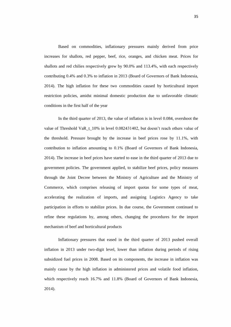
Based on commodities, inflationary pressures mainly derived from price

increases for shallots, red pepper, beef, rice, oranges, and chicken meat. Prices for

shallots and red chilies respectively grew by 90.0% and 113.4%, with each respectively

contributing 0.4% and 0.3% to inflation in 2013 (Board of Governors of Bank Indonesia,

2014). The high inflation for these two commodities caused by horticultural import

restriction policies, amidst minimal domestic production due to unfavorable climatic

conditions in the first half of the year

In the third quarter of 2013, the value of inflation is in level 0.084, overshoot the

value of Threshold VaR_t_10% in level 0.082431402, but doesn’t reach others value of

the threshold. Pressure brought by the increase in beef prices rose by 11.1%, with

contribution to inflation amounting to 0.1% (Board of Governors of Bank Indonesia,

2014). The increase in beef prices have started to ease in the third quarter of 2013 due to

government policies. The government applied, to stabilize beef prices, policy measures

through the Joint Decree between the Ministry of Agriculture and the Ministry of

Commerce, which comprises releasing of import quotas for some types of meat,

accelerating the realization of imports, and assigning Logistics Agency to take

participation in efforts to stabilize prices. In due course, the Government continued to

refine these regulations by, among others, changing the procedures for the import

mechanism of beef and horticultural products

Inflationary pressures that eased in the third quarter of 2013 pushed overall

inflation in 2013 under two-digit level, lower than inflation during periods of rising

subsidized fuel prices in 2008. Based on its components, the increase in inflation was

mainly cause by the high inflation in administered prices and volatile food inflation,

which respectively reach 16.7% and 11.8% (Board of Governors of Bank Indonesia,

2014).

36

However, volatile food inflation resumed a waning trend at the end of the year in

line with the positive impact brought about by various policy responses taken by Bank

Indonesia and the government. The decline in shallots and red chili prices was cause by

the Government’s policy response to relax restrictions on horticultural imports. This is in

line with Inflation Controlling Team’s recommendations in the need to relax regulations

and accelerate the realization of imports given the limited domestic supply. The impact of

the relaxation of policies on horticultural imports was also evident in commodity prices

for garlic that continued to deflate in the fourth quarter of 2013.

4.4.5 Value at Risk of Inflation Threshold in 2017

In the first quarter of 2017, the value of inflation is in level 0.0361 reach the

value of Threshold VaR_t_10% in level 0.036949983. According to Board of Governors

of Bank Indonesia (2017), Inflationary pressures stemmed from administered prices,

primarily the implementation of several tariff policies at beginning of 2017. In the first

quarter of 2017, the high inflationary pressure drove by the higher administration fees on

vehicle registration renewals and higher electricity tariffs. Inflationary pressures on

administered prices driven by phase II adjustments to electricity rates for nonsubsidised

900VA subscribers as well as higher airfares as seasonal demand continued to spike

during the long holidays.

4.4.6 Average Value at Risk of Inflations Threshold

The average value at risk of inflation threshold in this study is 10% (0.100038).

Similar result that found by Espinoza, Prasad and Leon (2010), and closer with

Widaryoko (2013) using a model of Hansen in 2000 found that inflation threshold in

Indonesia at 9.53%, also Chowdhury and Ham (2009) using threshold vector auto-

regression (TVAR) concluded threshold inflation in Indonesia is between on 8.50 to 11%.

37

CHAPTER V

CONCLUSIONS AND RECOMENDATIONS

5.1 Conclusions

This study aimed to examine the effect of the money supply, statutory reserve

requirement, GDP, interest rates, exchange rate, and Certificate of Bank Indonesia, to

describe the threshold of inflation in Indonesia during the period 2005 Q3 to 2013. This

study founds two variables as monetary transmission, rates and statutory reserve (GWM),

positively influence inflation by 13.05% and 3.17%. This indicate Bank Indonesia

monetary policy give enough impact to inflation and the decision to change the monetary

policy can do more carefully remind the impact will affected to inflation. Seen from the

negative impact of previous inflation to inflation, indicate Bank Indonesia as central bank

managed and controlled well to keep inflation keep on track. Moreover, this found

negative relationship between GDP and inflation by only 0.004%, indicate economic

growth in Indonesia closer to the inflation threshold because the coefficient level is below

0.0% is mean close to positive relationship with the inflation. All significant data justify

hypothesis that there is an influence from Reserve Requirements, Money Supply, Bank

Indonesia Certificate, Interest Rates and Exchange Rate to Inflation in Indonesia.

From the correlation between threshold and the value of inflation, Indonesia has

inflation trend caused by administered prices and volatile food. With 10% threshold,

indicate central government and central bank should keeping inflation low, stable, and

predictable, thus providing a climate that is more favorable to sound, sustained economic

growth and job creation and more carefully if want to raise the administered prices. The

administered prices can give highest inflationary pressure when the government

decreased subsidy and creating raise in administered price. For the volatile foods, usually

38

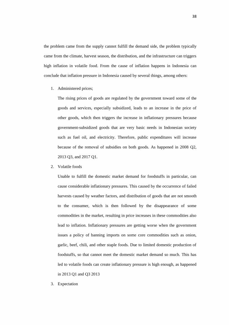
the problem came from the supply cannot fulfill the demand side, the problem typically

came from the climate, harvest season, the distribution, and the infrastructure can triggers

high inflation in volatile food. From the cause of inflation happens in Indonesia can

conclude that inflation pressure in Indonesia caused by several things, among others:

1. Administered prices;

The rising prices of goods are regulated by the government toward some of the

goods and services, especially subsidized, leads to an increase in the price of

other goods, which then triggers the increase in inflationary pressures because

government-subsidized goods that are very basic needs in Indonesian society

such as fuel oil, and electricity. Therefore, public expenditures will increase

because of the removal of subsidies on both goods. As happened in 2008 Q2,

2013 Q3, and 2017 Q1.

2. Volatile foods

Unable to fulfill the domestic market demand for foodstuffs in particular, can

cause considerable inflationary pressures. This caused by the occurrence of failed

harvests caused by weather factors, and distribution of goods that are not smooth

to the consumer, which is then followed by the disappearance of some

commodities in the market, resulting in price increases in these commodities also

lead to inflation. Inflationary pressures are getting worse when the government

issues a policy of banning imports on some core commodities such as onion,

garlic, beef, chili, and other staple foods. Due to limited domestic production of

foodstuffs, so that cannot meet the domestic market demand so much. This has

led to volatile foods can create inflationary pressure is high enough, as happened

in 2013 Q1 and Q3 2013

3. Expectation

39

Expectation inflation can also create quite high pressures, as happened in the 1st

quarter of 2012, when the fuel price hike became a hot issue of national news.

This has an impact on the people of Indonesia, which then make them speculate

about the fuel price hike, thus making inflation pressure almost high enough.

Some of the issues developing in society often lead to panic, which then have

resulted in rising prices of goods.

5.2 Recommendations

Therefore, if the government wants to raise the price of goods regulated by the

government, the government should coordinate with Bank Indonesia as the central bank

first to minimize the pressures that will occur in administered prices increase. In this case,

the central bank of Indonesian bank is in charge of tackling or minimizing inflationary

pressures from the monetary side so that inflationary pressures are less likely to affect

domestic economic performance. In the event of pressure, Bank Indonesia may update or

adjust monetary policy measures to minimize inflationary pressures, which may occur, so

as not to overstate or exceed the predetermined inflation target.

Given the domestic demand for staple foods commodity is enormous, even

greater than the production capacity that can produce domestically, so the frequent

occurrence of scarcity of staple foods commodity as well as uncertain whether factors can

exacerbate the situation that can making crop failure. This causes the government to

import food into the country considering the amount of domestic demand that cannot

meet without the help of imported foodstuffs. However, this should reconsider, as the

government must coordinate with the relevant ministries, since improper import decisions

can affect the rupiah exchange rate and can raise core inflation. The recommendation

from the researcher is that the government should pay more attention and increase the

40

production capacity and invest long-term in the improvement of research and

development to the field of horticulture, agriculture, and animal husbandry, because these

three sectors are very important in national food security.

As happened in the first quarter of 2012, the people of Indonesia shock by the

news about the planned increase in fuel prices made by the government at that time. This

price hike plan becomes a national issue and makes Indonesians speculate on the fuel

price hikes. This makes the sellers in the market began to raise the price of goods in order

to prepare the fuel price increase that be done by the government. The discourse of fuel

price hike by the government, has been heard by the public, this is what causes inflation

expectations in the wider community, and make the prices of goods on the market go up,

whereas this fuel price increase is just a discourse.

Estimating inflation threshold is interesting issue for economics since many

researchers always had different: method, variables, and results for estimating inflation

threshold. The fluctuation of inflation came from fluctuate economic activities. Doing an

estimating threshold inflation is challenging, because sometimes the inflation is caused by

a volatile economic conditions, which is not only one factor that can influence but also an

unexpected thing such as inflations expectations can creates major effect on Inflation.

41

REFERENCES

Ayyoub, M. (2016). Inflation-Growth Nexus in Developing Economies: New Empirical

Evidance from a Dis-aggregated Approach.

Aziz, E. B., & Nasrudin. (2016, December 26). Estimation Threshold Inflation in

Indonesia. Journal of Applied Economic Sciences, pp. 1376-1383.

Baglan, D., & Yoldas, E. (2014, July 28). Non-linearity in the Inflation-Growth

Relationship in Developing Economies: Evidence from a Semiparametric Panel

Model. Economics Letters.

Board of Governors of Bank Indonesia. (2009). 2008 Economic Report on Indonesia.

Jakarta: Bank Indonesia.

Board of Governors of Bank Indonesia. (2010). 2009 Economic Report on Indonesia.

Jakarta: Bank Indonesia.

Board of Governors of Bank Indonesia. (2014). 2013 Economic Report on Indonesia.

Jakarta: Bank Indonesia.

Caselli, F., Esquivel, G., & Lefort, F. (1996, September). Reopening the Convergence

Debate: New Look at Cross-Country Growth Empirics. Journal of Economic

Growth, pp. 363-389.

Chowdhury, A., & Ham, R. (2009). Inflation Targeting in Indonesia. The Singapore

Economic Review, 54, 645-655.

Chowdhury, A., & Siregar, H. (2004). Indonesia's Monetary Policy Dilemma: Constraints

of Inflation Targeting. The Journal of Developing Areas, pp. 137-153.

Drukker, D., Porqueras, P. G., & Verme, P. H. (2005, February 9). Threshold Effects in the

Relationship Between Inflation and Growth: A New Panel-Data Approach.

Espinoza, R., Leon, H., & Prasad, A. (2010, March). Estimating The Inflation-Growth

Nexus—A Smooth Transition Model. IMF Working Paper.

Fischer, S. (1993). The Role of Macroeconomic Factors in Growth. NBER Working Paper

Series.

Frimpong, J. M., & Oteng-Abaiye, E. F. (2010). When is Inflation Harmful? Estimating the

Threshold Effect for Ghana. American Journal of Economics and Business

Administration, 232-239.

Hansen, B. E. (1997, April). Inference in TAR Models. Studies in Nonlinear Dynamics and

Econometrics.

Hansen, B. E. (1999, April 1). Threshold e!ects in non-dynamic panels: Estimation,

testing, and inference. Journal of Econometrics, pp. 345-368.

42

Hansen, B. E. (2000). Sample Splitting and Threshold Estimation. Econometrica, 575-603.

Keynes, J. M. (1936). The General Theory of Employment, Interest, and Money. London:

Palgrave Macmillan.

Khan, M. S., & Senhadji, A. S. (2000). Threshold Effects in the Relationship Between

Inflation and Growth. IMF Working Paper.

Kremer, S., Bick, A., & Nautz, D. (2013, April). Inflation and growth: new evidence from a

dynamic. Empirical Economics, pp. 861-878.

Langi, T. M., Masinambow, V., & Siwu, H. (2014). Analisis Pengaruh Suku Bunga BI,

Jumlah Uang Beredar, dan Tingkat Kurs Terhadap Tingkat Inflasi di Indonesia.

Jurnal Berkala Ilmiah Efisiensi, 14, 44-58.

Larasati, D. M., & Amri. (2017, November 4). Pengaruh Tingkat Suku Bunga Sertifikat

Bank Indonesia dan Nilai Tukar Terhadap Inflasi di Indonesia. Jurnal Ilmiah

Mahasiswa (JIM) Ekonomi Pembangunan Fakultas Ekonomi dan Bisnis Unsyiah,

2, 535-543.

Lin, S., & Ye, H. (2009). Does inflation targeting make a difference in developing

countries? Journal of Development Economics, pp. 118-123.

Mubarik, Y. A. (2005). Inflation and Growth: An Estimate of the Threshold LEvel of

Inflation in Pakistan. SBP-Research Bulletin, 1.

Munir, Q., & Mansur, K. (2009). Non-Linearity between Inflation Rate and GDP Growth

in Malaysia. Economics Bulletin, 1555-1569.

Nguyen, V. B. (2015, January 13). Effects of fiscal deficit and money M2 supply on

inflation: Evidance from selected economies of Asia. Journal of Economics,

Finance and Administrative Science, 20, 49-53.

Salami, D., & Kelikume, I. (2010, November). An Estimation of Inflation Threshold for

Nigeria 1970-2008. International Review of Business Research Papers, 6, pp. 375-

385.

Sarel, M. (1996). Nonlinear Effects of Inflation on Economic Growth. Palgrave Macmillan

Journals, 199-215.

Sepehri, A., & Moshiri, S. (2004, April). Inflation-Growth Profiles Across Countries:

Evidance from Developing and Developed Countries. International Review of

Applied Economics, pp. 191-207.

Setyawan, A. R. (2010, July). Efektifitas Kebijakan Moneter Terhadap Inflasi di Indonesia.

Jurnal Ekonomi Pembangunan, 8(1), 281-292.

Subekti, A. (2011). Dinamika inflasi Indonesia pada provinsi. Bogor: Institut Pertanian

Bogor.

43

Sutawijaya, A. (2012). Pengaruh Faktor-Faktor Ekonomi Terhadap Inflasi di Indonesia.

Jurnal Organisasi dan Manajemen, 8, 85-101.

Vinayagathasan, T. (2013, April 13). Inflation and economic growth: A dynamic panel

threshold analysis for Asian economies. Journal of Asian Economics, pp. 31-41.

Widaryoko, N. (2013). Inflasi dan Pertumbuhan Ekonomi: Pendugaan Ambang Batas

Inflasi di Indonesia. Bogor: Institut Pertanian Bogor.

Winarno, T. (2014). The Dynamics Relationship Between Inflationand Economics Growth

in Indonesia: A Regional Thresholds Approach.

44

APPENDICES

45

Appendix 1 Inflation, M2. Reserve Requirement (GWM), Rate, Exchange Rate

(ER), Bank Indonesia’s Certificate (SBI)

Date Inflation M2 GWM GDP Rate ER SBI

2005 Q3 9.06% 1154 5.00% 713 10.00% 10310 50

2005 Q4 17.11% 1203 5.00% 758 12.75% 9830 69

2006 Q1 15.74% 1199 5.00% 783 12.75% 9075 1317

2006 Q2 15.53% 1258 5.00% 813 12.50% 9300 168

2006 Q3 14.55% 1295 5.00% 870 11.25% 9235 183

2006 Q4 6.60% 1382 5.00% 873 9.75% 9020 209

2007 Q1 6.52% 1379 5.00% 920 9.00% 9118 244

2007 Q2 5.78% 1455 5.00% 964 8.50% 9054 260

2007 Q3 6.95% 1517 5.00% 1031 8.25% 9137 263

2007 Q4 6.59% 1650 5.00% 1035 8.00% 9419 274

2008 Q1 8.17% 1594 5.00% 1110 7.96% 9217 261

2008 Q2 11.03% 1703 5.00% 1221 8.52% 9225 165

2008 Q3 12.14% 1778 5.00% 1328 9.40% 9378 136

2008 Q4 11.06% 1896 5.00% 1291 9.49% 10950 169

2009 Q1 7.92% 1917 5.00% 1315 8.22% 11575 234

2009 Q2 3.65% 1978 5.00% 1381 6.84% 10225 231

2009 Q3 2.83% 2019 5.00% 1458 6.37% 9681 217

2009 Q4 2.78% 2141 5.00% 1451 6.50% 9400 254

2010 Q1 3.43% 2112 5.00% 1604 6.19% 9115 298

2010 Q2 5.05% 2231 5.00% 1705 6.28% 9083 270

2010 Q3 5.80% 2275 5.00% 1786 6.26% 8924 252

2010 Q4 6.96% 2471 8.00% 1770 5.78% 8991 200

2011 Q1 6.65% 2451 8.00% 1834 6.17% 8709 230

2011 Q2 5.54% 2523 8.00% 1928 6.37% 8597 186

2011 Q3 4.61% 2643 8.00% 2054 5.34% 8823 149

2011 Q4 3.79% 2877 8.00% 2015 4.57% 9068 120

2012 Q1 3.97% 2914 8.00% 2061 3.78% 9180 94

2012 Q2 4.53% 3053 8.00% 2162 4.14% 9480 90

2012 Q3 4.31% 3128 8.00% 2224 4.19% 9588 68

2012 Q4 4.30% 3308 8.00% 2169 4.49% 9670 79

2013 Q1 5.90% 3323 8.00% 2235 4.30% 9719 92

2013 Q2 5.90% 3413 8.00% 2343 4.59% 9929 82

2013 Q3 8.40% 3584 8.00% 2491 5.83% 11613 65

2013 Q4 8.38% 3730 8.00% 2477 6.74% 12189 91

2014 Q1 7.32% 3653 8.00% 2506 6.27% 11404 104

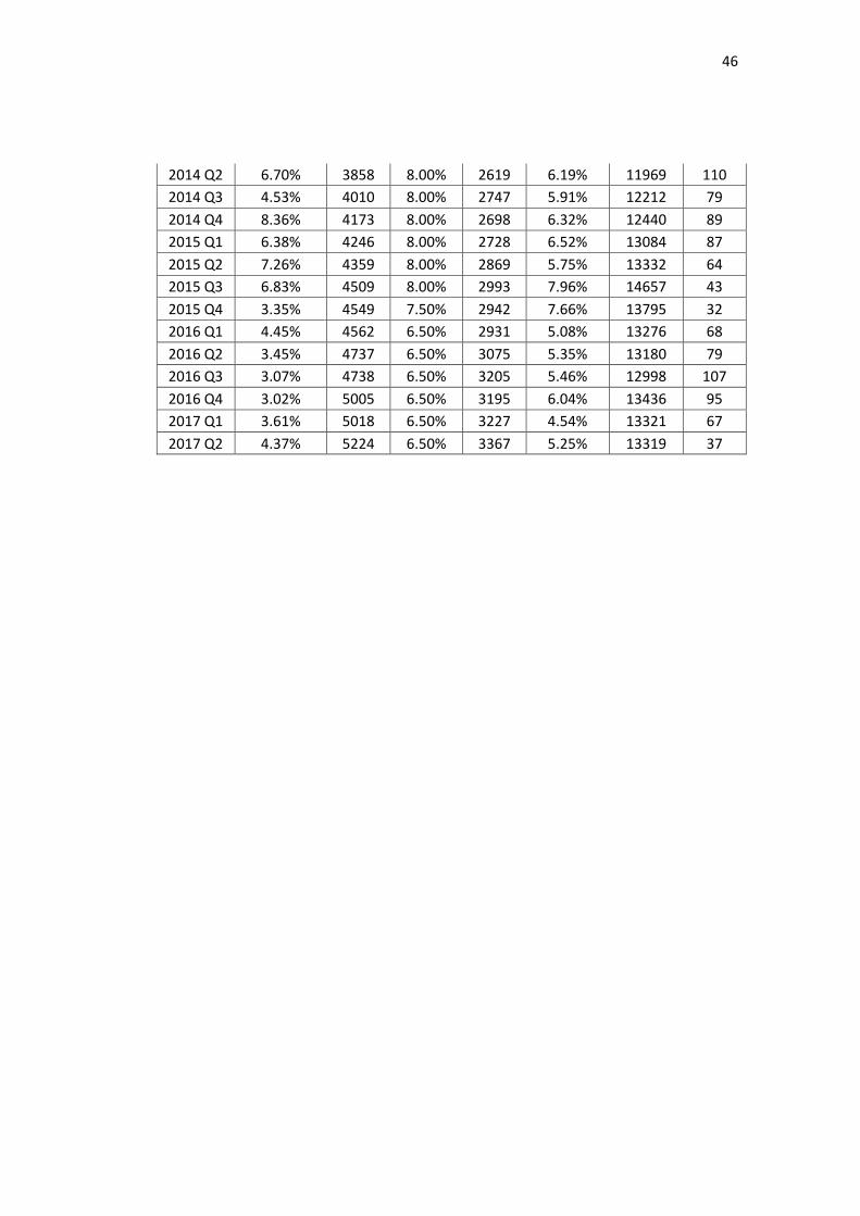
46

2014 Q2 6.70% 3858 8.00% 2619 6.19% 11969 110

2014 Q3 4.53% 4010 8.00% 2747 5.91% 12212 79

2014 Q4 8.36% 4173 8.00% 2698 6.32% 12440 89

2015 Q1 6.38% 4246 8.00% 2728 6.52% 13084 87

2015 Q2 7.26% 4359 8.00% 2869 5.75% 13332 64

2015 Q3 6.83% 4509 8.00% 2993 7.96% 14657 43

2015 Q4 3.35% 4549 7.50% 2942 7.66% 13795 32

2016 Q1 4.45% 4562 6.50% 2931 5.08% 13276 68

2016 Q2 3.45% 4737 6.50% 3075 5.35% 13180 79

2016 Q3 3.07% 4738 6.50% 3205 5.46% 12998 107

2016 Q4 3.02% 5005 6.50% 3195 6.04% 13436 95

2017 Q1 3.61% 5018 6.50% 3227 4.54% 13321 67

2017 Q2 4.37% 5224 6.50% 3367 5.25% 13319 37

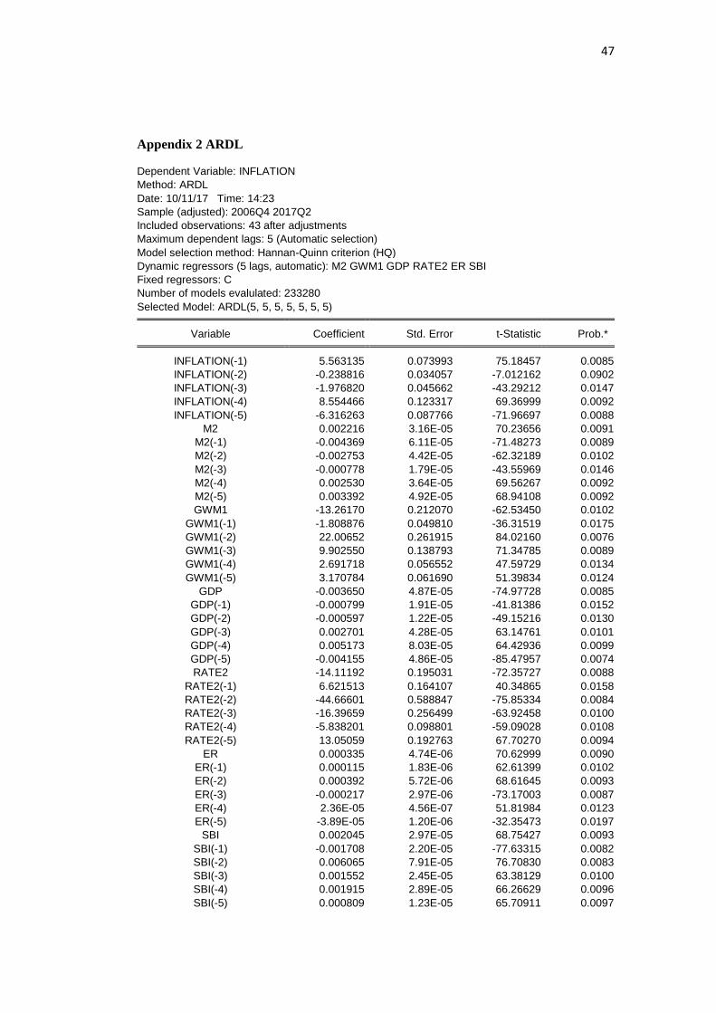
47

Appendix 2 ARDL

Dependent Variable: INFLATION

Method: ARDL

Date: 10/11/17 Time: 14:23

Sample (adjusted): 2006Q4 2017Q2

Included observations: 43 after adjustments

Maximum dependent lags: 5 (Automatic selection)

Model selection method: Hannan-Quinn criterion (HQ)

Dynamic regressors (5 lags, automatic): M2 GWM1 GDP RATE2 ER SBI

Fixed regressors: C

Number of models evalulated: 233280

Selected Model: ARDL(5, 5, 5, 5, 5, 5, 5) Variable Coefficient Std. Error t-Statistic Prob.* INFLATION(-1) 5.563135 0.073993 75.18457 0.0085

INFLATION(-2) -0.238816 0.034057 -7.012162 0.0902

INFLATION(-3) -1.976820 0.045662 -43.29212 0.0147

INFLATION(-4) 8.554466 0.123317 69.36999 0.0092

INFLATION(-5) -6.316263 0.087766 -71.96697 0.0088

M2 0.002216 3.16E-05 70.23656 0.0091

M2(-1) -0.004369 6.11E-05 -71.48273 0.0089

M2(-2) -0.002753 4.42E-05 -62.32189 0.0102

M2(-3) -0.000778 1.79E-05 -43.55969 0.0146

M2(-4) 0.002530 3.64E-05 69.56267 0.0092

M2(-5) 0.003392 4.92E-05 68.94108 0.0092

GWM1 -13.26170 0.212070 -62.53450 0.0102

GWM1(-1) -1.808876 0.049810 -36.31519 0.0175

GWM1(-2) 22.00652 0.261915 84.02160 0.0076

GWM1(-3) 9.902550 0.138793 71.34785 0.0089

GWM1(-4) 2.691718 0.056552 47.59729 0.0134

GWM1(-5) 3.170784 0.061690 51.39834 0.0124

GDP -0.003650 4.87E-05 -74.97728 0.0085

GDP(-1) -0.000799 1.91E-05 -41.81386 0.0152

GDP(-2) -0.000597 1.22E-05 -49.15216 0.0130

GDP(-3) 0.002701 4.28E-05 63.14761 0.0101

GDP(-4) 0.005173 8.03E-05 64.42936 0.0099

GDP(-5) -0.004155 4.86E-05 -85.47957 0.0074

RATE2 -14.11192 0.195031 -72.35727 0.0088

RATE2(-1) 6.621513 0.164107 40.34865 0.0158

RATE2(-2) -44.66601 0.588847 -75.85334 0.0084

RATE2(-3) -16.39659 0.256499 -63.92458 0.0100

RATE2(-4) -5.838201 0.098801 -59.09028 0.0108

RATE2(-5) 13.05059 0.192763 67.70270 0.0094

ER 0.000335 4.74E-06 70.62999 0.0090

ER(-1) 0.000115 1.83E-06 62.61399 0.0102

ER(-2) 0.000392 5.72E-06 68.61645 0.0093

ER(-3) -0.000217 2.97E-06 -73.17003 0.0087

ER(-4) 2.36E-05 4.56E-07 51.81984 0.0123

ER(-5) -3.89E-05 1.20E-06 -32.35473 0.0197

SBI 0.002045 2.97E-05 68.75427 0.0093

SBI(-1) -0.001708 2.20E-05 -77.63315 0.0082

SBI(-2) 0.006065 7.91E-05 76.70830 0.0083

SBI(-3) 0.001552 2.45E-05 63.38129 0.0100

SBI(-4) 0.001915 2.89E-05 66.26629 0.0096

SBI(-5) 0.000809 1.23E-05 65.70911 0.0097

48

C -2.292454 0.033468 -68.49659 0.0093 R-squared 0.999995 Mean dependent var 0.058660

Adjusted R-squared 0.999801 S.D. dependent var 0.022763

S.E. of regression 0.000321 Akaike info criterion -15.05814

Sum squared resid 1.03E-07 Schwarz criterion -13.33790

Log likelihood 365.7500 Hannan-Quinn criter. -14.42377

F-statistic 5152.318 Durbin-Watson stat 3.497113

Prob(F-statistic) 0.011048 *Note: p-values and any subsequent tests do not account for model

selection.

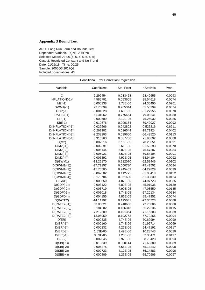
49

Appendix 3 Bound Test

ARDL Long Run Form and Bounds Test

Dependent Variable: D(INFLATION)

Selected Model: ARDL(5, 5, 5, 5, 5, 5, 5)

Case 2: Restricted Constant and No Trend

Date: 01/22/18 Time: 00:25

Sample: 2005Q3 2017Q2

Included observations: 43 Conditional Error Correction Regression Variable Coefficient Std. Error t-Statistic Prob. C -2.292454 0.033468 -68.49655 0.0093

INFLATION(-1)* 4.585701 0.053605 85.54618 0.0074

M2(-1) 0.000238 9.78E-06 24.35490 0.0261

GWM1(-1) 22.70099 0.265344 85.55299 0.0074

GDP(-1) -0.001328 1.63E-05 -81.27955 0.0078

RATE2(-1) -61.34062 0.775654 -79.08241 0.0080

ER(-1) 0.000609 8.10E-06 75.26032 0.0085

SBI(-1) 0.010676 0.000154 69.42027 0.0092

D(INFLATION(-1)) -0.022566 0.042802 -0.527216 0.6911

D(INFLATION(-2)) -0.261382 0.016544 -15.79924 0.0402

D(INFLATION(-3)) -2.238203 0.039660 -56.43520 0.0113

D(INFLATION(-4)) 6.316263 0.087766 71.96692 0.0088

D(M2) 0.002216 3.16E-05 70.23651 0.0091

D(M2(-1)) -0.002391 2.61E-05 -91.59293 0.0070

D(M2(-2)) -0.005144 6.82E-05 -75.47287 0.0084

D(M2(-3)) -0.005921 8.50E-05 -69.64104 0.0091

D(M2(-4)) -0.003392 4.92E-05 -68.94104 0.0092

D(GWM1) -13.26170 0.212070 -62.53446 0.0102

D(GWM1(-1)) -37.77157 0.500780 -75.42552 0.0084

D(GWM1(-2)) -15.76505 0.245453 -64.22829 0.0099

D(GWM1(-3)) -5.862502 0.112775 -51.98419 0.0122

D(GWM1(-4)) -3.170784 0.061690 -51.39830 0.0124

D(GDP) -0.003650 4.87E-05 -74.97723 0.0085

D(GDP(-1)) -0.003122 6.80E-05 -45.91936 0.0139

D(GDP(-2)) -0.003719 7.90E-05 -47.08550 0.0135

D(GDP(-3)) -0.001018 3.74E-05 -27.20134 0.0234

D(GDP(-4)) 0.004155 4.86E-05 85.47952 0.0074

D(RATE2) -14.11192 0.195031 -72.35723 0.0088

D(RATE2(-1)) 53.85021 0.740636 72.70806 0.0088

D(RATE2(-2)) 9.184202 0.166313 55.22236 0.0115

D(RATE2(-3)) -7.212389 0.101364 -71.15303 0.0089

D(RATE2(-4)) -13.05059 0.192763 -67.70266 0.0094

D(ER) 0.000335 4.74E-06 70.62994 0.0090

D(ER(-1)) -0.000160 1.74E-06 -91.92714 0.0069

D(ER(-2)) 0.000232 4.27E-06 54.47192 0.0117

D(ER(-3)) 1.53E-05 1.49E-06 10.23743 0.0620

D(ER(-4)) 3.89E-05 1.20E-06 32.35471 0.0197

D(SBI) 0.002045 2.97E-05 68.75423 0.0093

D(SBI(-1)) -0.010339 0.000144 -71.69380 0.0089

D(SBI(-2)) -0.004275 6.56E-05 -65.13242 0.0098

D(SBI(-3)) -0.002723 4.12E-05 -66.14883 0.0096

D(SBI(-4)) -0.000809 1.23E-05 -65.70906 0.0097

50

* p-value incompatible with t-Bounds distribution.

Levels Equation

Case 2: Restricted Constant and No Trend Variable Coefficient Std. Error t-Statistic Prob. M2 -5.20E-05 2.27E-06 -22.84665 0.0278

GWM1 -4.950386 0.030644 -161.5427 0.0039

GDP 0.000290 3.52E-06 82.30596 0.0077

RATE2 13.37650 0.089132 150.0751 0.0042

ER -0.000133 1.00E-06 -132.3590 0.0048

SBI -0.002328 2.08E-05 -111.8248 0.0057

C 0.499914 0.004459 112.1227 0.0057 EC = INFLATION - (-0.0001*M2 -4.9504*GWM1 + 0.0003*GDP + 13.3765

*RATE2 -0.0001*ER -0.0023*SBI + 0.4999 )

F-Bounds Test Null Hypothesis: No levels relationship Test Statistic Value Signif. I(0) I(1)

Asymptotic:

n=1000

F-statistic 2680.786 10% 1.99 2.94

k 6 5% 2.27 3.28

2.5% 2.55 3.61

1% 2.88 3.99

Actual Sample Size 43 Finite Sample:

n=45

10% 2.188 3.254

5% 2.591 3.766

1% 3.54 4.931

Finite Sample:

n=40

10% 2.218 3.314

5% 2.618 3.863

1% 3.505 5.121

51

Appendix 4 Error Correction Model

ARDL Error Correction Regression

Dependent Variable: D(INFLATION)

Selected Model: ARDL(5, 5, 5, 5, 5, 5, 5)

Case 2: Restricted Constant and No Trend

Date: 01/22/18 Time: 00:29

Sample: 2005Q3 2017Q2

Included observations: 43 ECM Regression

Case 2: Restricted Constant and No Trend Variable Coefficient Std. Error t-Statistic Prob. D(INFLATION(-1)) -0.022566 0.003546 -6.363707 0.0992

D(INFLATION(-2)) -0.261382 0.003531 -74.02732 0.0086

D(INFLATION(-3)) -2.238203 0.005029 -445.0184 0.0014

D(INFLATION(-4)) 6.316263 0.016145 391.2101 0.0016

D(M2) 0.002216 5.62E-06 394.4847 0.0016

D(M2(-1)) -0.002391 5.97E-06 -400.2343 0.0016

D(M2(-2)) -0.005144 1.26E-05 -409.8383 0.0016

D(M2(-3)) -0.005921 1.46E-05 -406.9608 0.0016

D(M2(-4)) -0.003392 8.04E-06 -421.9570 0.0015

D(GWM1) -13.26170 0.032907 -403.0038 0.0016

D(GWM1(-1)) -37.77157 0.091447 -413.0443 0.0015

D(GWM1(-2)) -15.76505 0.038457 -409.9443 0.0016

D(GWM1(-3)) -5.862502 0.014980 -391.3468 0.0016

D(GWM1(-4)) -3.170784 0.008222 -385.6595 0.0017

D(GDP) -0.003650 8.85E-06 -412.2647 0.0015

D(GDP(-1)) -0.003122 7.90E-06 -394.9720 0.0016

D(GDP(-2)) -0.003719 8.91E-06 -417.4859 0.0015

D(GDP(-3)) -0.001018 3.03E-06 -336.2257 0.0019

D(GDP(-4)) 0.004155 1.07E-05 388.9413 0.0016

D(RATE2) -14.11192 0.038358 -367.8999 0.0017

D(RATE2(-1)) 53.85021 0.133567 403.1694 0.0016

D(RATE2(-2)) 9.184202 0.020489 448.2484 0.0014

D(RATE2(-3)) -7.212389 0.019710 -365.9289 0.0017

D(RATE2(-4)) -13.05059 0.032709 -398.9908 0.0016

D(ER) 0.000335 8.07E-07 414.6145 0.0015

D(ER(-1)) -0.000160 3.68E-07 -434.2847 0.0015

D(ER(-2)) 0.000232 5.81E-07 400.0723 0.0016

D(ER(-3)) 1.53E-05 9.45E-08 161.5502 0.0039

D(ER(-4)) 3.89E-05 1.09E-07 357.3612 0.0018

D(SBI) 0.002045 5.68E-06 360.1967 0.0018

D(SBI(-1)) -0.010339 2.47E-05 -418.3348 0.0015

D(SBI(-2)) -0.004275 1.03E-05 -413.2025 0.0015

D(SBI(-3)) -0.002723 6.51E-06 -418.3745 0.0015

D(SBI(-4)) -0.000809 1.87E-06 -432.5694 0.0015

CointEq(-1)* 4.585701 0.011071 414.2105 0.0015 R-squared 0.999994 Mean dependent var -0.002367

Adjusted R-squared 0.999967 S.D. dependent var 0.019692

S.E. of regression 0.000113 Akaike info criterion -15.38372

Sum squared resid 1.03E-07 Schwarz criterion -13.95018

Log likelihood 365.7500 Hannan-Quinn criter. -14.85508

Durbin-Watson stat 3.497113

52

* p-value incompatible with t-Bounds distribution.

F-Bounds Test Null Hypothesis: No levels relationship Test Statistic Value Signif. I(0) I(1) F-statistic 2680.786 10% 1.99 2.94

k 6 5% 2.27 3.28

2.5% 2.55 3.61

1% 2.88 3.99

53

Appendix 4 GARCH

Dependent Variable: INFLATION

Method: ML - ARCH

Date: 10/11/17 Time: 14:23

Sample: 2005Q3 2017Q2

Included observations: 48

Failure to improve likelihood (non-zero gradients) after 57 iterations

Coefficient covariance computed using outer product of gradients

Presample variance: backcast (parameter = 0.7)

GARCH = C(8) + C(9)*RESID(-1)^2 + C(10)*RESID(-1)^2*(RESID(-1)<0) +

C(11)*GARCH(-1) Variable Coefficient Std. Error z-Statistic Prob. C -0.054823 0.000178 -307.7224 0.0000

M2 -3.02E-06 9.39E-06 -0.321390 0.7479

GWM1 0.734629 0.171894 4.273733 0.0000

GDP 1.02E-05 1.46E-05 0.698682 0.4848

RATE2 1.728349 0.020440 84.55772 0.0000

ER -4.65E-06 6.15E-07 -7.557484 0.0000

SBI -2.14E-05 8.93E-06 -2.395842 0.0166 Variance Equation C 1.04E-05 1.82E-05 0.570017 0.5687

RESID(-1)^2 0.260015 0.379177 0.685737 0.4929

RESID(-1)^2*(RESID(-1)<0) -0.568354 0.411018 -1.382798 0.1667

GARCH(-1) 1.112377 0.064896 17.14087 0.0000 R-squared 0.752593 Mean dependent var 0.067548

Adjusted R-squared 0.716387 S.D. dependent var 0.035209

S.E. of regression 0.018751 Akaike info criterion -5.083218

Sum squared resid 0.014415 Schwarz criterion -4.654401

Log likelihood 132.9972 Hannan-Quinn criter. -4.921167

Durbin-Watson stat 1.221563

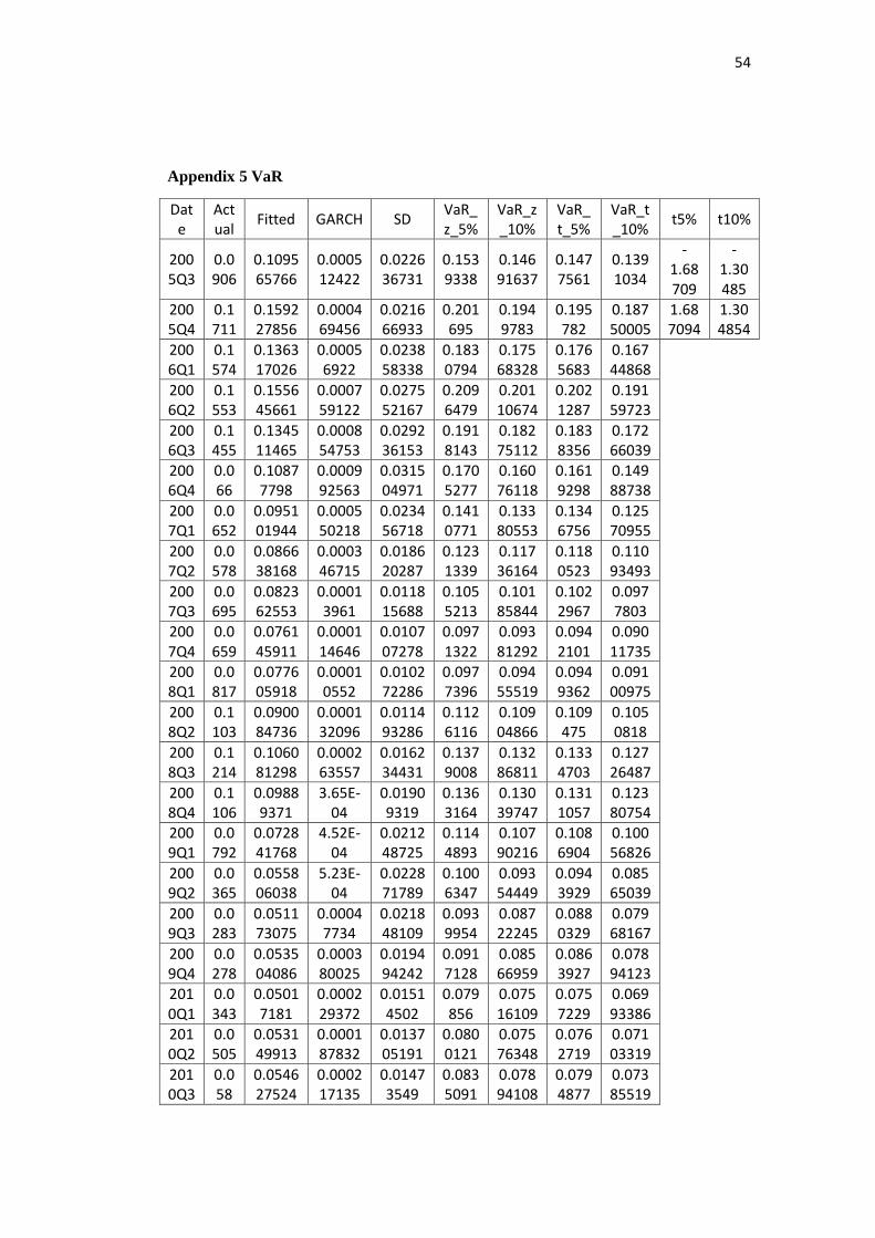
54

Appendix 5 VaR

Date

Actual

Fitted GARCH SD VaR_z_5%

VaR_z_10%

VaR_t_5%

VaR_t_10%

t5% t10%

2005Q3

0.0906

0.109565766

0.000512422

0.022636731

0.1539338

0.14691637

0.1477561

0.1391034

-1.68709

-1.30485

2005Q4

0.1711

0.159227856

0.000469456

0.021666933

0.201695

0.1949783

0.195782

0.18750005

1.687094

1.304854

2006Q1

0.1574

0.136317026

0.00056922

0.023858338

0.1830794

0.17568328

0.1765683

0.16744868

2006Q2

0.1553

0.155645661

0.000759122

0.027552167

0.2096479

0.20110674

0.2021287

0.19159723

2006Q3

0.1455

0.134511465

0.000854753

0.029236153

0.1918143

0.18275112

0.1838356

0.17266039

2006Q4

0.066

0.10877798

0.000992563

0.031504971

0.1705277

0.16076118

0.1619298

0.14988738

2007Q1

0.0652

0.095101944

0.000550218

0.023456718

0.1410771

0.13380553

0.1346756

0.12570955

2007Q2

0.0578

0.086638168

0.000346715

0.018620287

0.1231339

0.11736164

0.1180523

0.11093493

2007Q3

0.0695

0.082362553

0.00013961

0.011815688

0.1055213

0.10185844

0.1022967

0.0977803

2007Q4

0.0659

0.076145911

0.000114646

0.010707278

0.0971322

0.09381292

0.0942101

0.09011735

2008Q1

0.0817

0.077605918

0.00010552

0.010272286

0.0977396

0.09455519

0.0949362

0.09100975

2008Q2

0.1103

0.090084736

0.000132096

0.011493286

0.1126116

0.10904866

0.109475

0.1050818

2008Q3

0.1214

0.106081298

0.000263557

0.016234431

0.1379008

0.13286811

0.1334703

0.12726487

2008Q4

0.1106

0.09889371

3.65E-04

0.01909319

0.1363164

0.13039747

0.1311057

0.12380754

2009Q1

0.0792

0.072841768

4.52E-04

0.021248725

0.1144893

0.10790216

0.1086904

0.10056826

2009Q2

0.0365

0.055806038

5.23E-04

0.022871789

0.1006347

0.09354449

0.0943929

0.08565039

2009Q3

0.0283

0.051173075

0.00047734

0.021848109

0.0939954

0.08722245

0.0880329

0.07968167

2009Q4

0.0278

0.053504086

0.000380025

0.019494242

0.0917128

0.08566959

0.0863927

0.07894123

2010Q1

0.0343

0.05017181

0.000229372

0.01514502

0.079856

0.07516109

0.0757229

0.06993386

2010Q2

0.0505

0.053149913

0.000187832

0.013705191

0.0800121

0.07576348

0.0762719

0.07103319

2010Q3

0.058

0.054627524

0.000217135

0.01473549

0.0835091

0.07894108

0.0794877

0.07385519

55

2010Q4

0.0696

0.068402774

0.000254852

0.015964099

0.0996924

0.09474354

0.0953357

0.0892336

2011Q1

0.0665

0.076532043

0.000294224

0.017152967

0.1101519

0.10483444

0.1054707

0.09891417

2011Q2

0.0554

0.082197988

0.000306616

0.017510456

0.1165185

0.11109024

0.1117398

0.10504658

2011Q3

0.0461

0.065049431

1.30E-04

0.011401934

0.0873972

0.08386262

0.0842856

0.0799273

2011Q4

0.0379

0.050134736

4.43E-05

0.006652402

0.0631734

0.0611112

0.061358

0.05881515

2012Q1

0.0397

0.036858821

1.34E-05

0.003665005

0.0440422

0.04290608

0.043042

0.04164112

2012Q2

0.0453

0.04239896

2.74E-05

0.005234515

0.0526586

0.05103591

0.0512301

0.04922924

2012Q3

0.0431

0.043623845

4.30E-05

0.006559504

0.0564805

0.05444703

0.0546903

0.05218304

2012Q4

0.043

0.047096497

5.81E-05

0.007624778

0.0620411

0.05967738

0.0599602

0.05704572

2013Q1

0.059

0.043939136

6.99E-05

0.008357972

0.0603208

0.05772979

0.0580398

0.05484507

2013Q2

0.059

0.049012934

1.47E-04

0.012126194

0.0727803

0.06902115

0.069471

0.06483585

2013Q3

0.084

0.063984302

2.00E-04

0.014137286

0.0916934

0.08731082

0.0878352

0.0824314

2013Q4

0.0838

0.075885269

3.37E-04

0.018353525

0.1118582

0.10616859

0.1068494

0.09983395

2014Q1

0.0732

0.071683857

4.01E-04

0.020033821

0.1109501

0.10473966

0.1054828

0.09782508

2014Q2

0.067

0.068068357

0.000457414

0.021387245

0.1099874

0.10335731

0.1041506

0.0959756

2014Q3

0.0453

0.063604444

0.000518825

0.022777726

0.1082488

0.10118769

0.1020326

0.09332606

2014Q4

0.0836

0.068429317

0.000484179

0.022004059

0.1115573

0.10473601

0.1055522

0.09714141

2015Q1

0.0638

0.069020001

0.000608791

0.024673695

0.1173804

0.1097316

0.1106468

0.10121558

2015Q2

0.0726

0.056147149

0.000679163

0.026060761

0.1072262

0.0991474

0.1001141

0.09015265

2015Q3

0.0683

0.08946332

0.00083623

0.02891765

0.1461419

0.13717744

0.1382501

0.12719664

2015Q4

0.0335

0.084192048

0.000802463

0.02832777

0.1397145

0.13093287

0.1319836

0.12115566

2016Q1

0.0445

0.033765402

0.000110667

0.010519836

0.0543843

0.05112313

0.0515133

0.04749226

2016Q2

0.0345

0.039578543

0.000163425

0.012783774

0.0646347

0.06067177

0.061146

0.05625951

56

2016Q3

0.0307

0.043038287

0.000184197

0.013571921

0.0696393

0.06543196

0.0659354

0.06074767

2016Q4

0.0302

0.050387531

0.000168317

0.01297369

0.075816

0.07179412

0.0722754

0.06731631

2017Q1

0.0361

0.025883177

7.19E-05

0.008481257

0.0425064

0.03987725

0.0401919

0.03694998

2017Q2

0.0437

0.039602959

1.18E-04

0.01084048

0.0608503

0.05748975

0.0578919

0.05374821