estimating hedonic demand parameters in real estate market
26
Muğla Üniversitesi Sosyal Bilimler Enstitüsü Dergisi (İLKE) Bahar 2008 Sayı 20 ESTIMATING HEDONIC DEMAND PARAMETERS IN REAL ESTATE MARKET: THE CASE OF MUGLA Ercan BALDEMİR Cüneyt Yenal KESBİÇ Mustafa İNCİ ABSTRACT The affect of each characteristic of a heterogeneous good on its price can be determined by Hedonic Price Models. This feature is originated from the assumption of the model that the price of a heterogeneous good is the sum of the prices of the characteristics constituting that good. Therefore, marginal prices for heterogeneous goods enter into the scene. In this respect, we examine the marginal effects of different housing attributes on the selling price of houses in the housing market in Mugla. 178 observations have been obtained through a questionnaire based on face to face interviews with randomly selected real estate agencies from the urban districts of Mugla. The analyses have been carried out by linear, logarithmic and logarithmic-linear functional forms, which are frequently used in Hedonic Price Models. Considering the structure and features of Mugla, the estimated coefficients are found to be significant in terms of both the characteristics of housing and its location (its position, whether it is in-site or not, etc.). As expected, the variables that positively affect the housing price have been found in all linear, logarithmic, and log-linear models to be central heating, ceramic bathroom floor, location on the street, satellite TV, hydrophor pump, modular kitchen, sunblind, solar water heating, front side facing south, 1500- 2000 meters to the city center, the number of bathrooms, square meter of housing, and elevator. Key Words: Hedonic theory, house markets, hedonic price model. Emlak Piyasasında Hedonik Talep Parametrelerinin Tahminlenmesi: Muğla Örneği ÖZET Hedonik Fiyatlandırma Modeli ile heterojen bir malı oluşturan karakteristiklerin her birinin fiyat üzerindeki etkisi tanımlanabilir. Bu durum, Model‘in, heterojen bir malın fiyatının, onu oluşturan farklı niteliklerin piyasa fiyatlarının toplamından ibaret olduğunu varsaymasından ileri gelir. Böylece heterojen mallar için marjinal fiyatlar söz konusu olmaktadır. Bu bağlamda, çalışmada Muğla Konut Piyasasında konutların sahip olduğu farklı niteliklerin konut satış fiyatı üzerindeki marjinal etkisi ortaya konmaya çalışılmıştır. Muğla ili kentsel kesimde merkez ilçelerde emlak bürolarında emlakçılarla yüz yüze görüşme suretiyle tesadüfi olarak 178 anket yapılmıştır. Analizler hedonik fiyat modelinde sıklıkla benimsenen doğrusal, logaritmik ve logaritmik doğrusal fonksiyonlar kullanılarak gerçekleştirilmiştir. Katsayı tahminleri gerek konutun özellikleri, gerekse konumu (konutun yeri, site içinde olup olmaması vb.) açısından Muğla ilinin yapısı ve özellikleri dikkate alındığında anlamlı çıkmıştır. Beklendiği gibi, doğrusal, logaritmik ve logaritmik doğrusal modellerin Associate Professor, Mugla University, F.E.A.S., Department of Business Administration. Associate Professor, Mugla University, F.E.A.S., Department of Economics. Research Assistant, Mugla University, F.E.A.S., Department of Economics.
Transcript of estimating hedonic demand parameters in real estate market

Muğla Üniversitesi
Sosyal Bilimler Enstitüsü Dergisi (İLKE)
Bahar 2008 Sayı 20
ESTIMATING HEDONIC DEMAND PARAMETERS IN REAL
ESTATE MARKET: THE CASE OF MUGLA
Ercan BALDEMİR
Cüneyt Yenal KESBİÇ
Mustafa İNCİ
ABSTRACT
The affect of each characteristic of a heterogeneous good on its price can be determined
by Hedonic Price Models. This feature is originated from the assumption of the model that the
price of a heterogeneous good is the sum of the prices of the characteristics constituting that good.
Therefore, marginal prices for heterogeneous goods enter into the scene. In this respect, we
examine the marginal effects of different housing attributes on the selling price of houses in the
housing market in Mugla.
178 observations have been obtained through a questionnaire based on face to face
interviews with randomly selected real estate agencies from the urban districts of Mugla. The
analyses have been carried out by linear, logarithmic and logarithmic-linear functional forms,
which are frequently used in Hedonic Price Models. Considering the structure and features of
Mugla, the estimated coefficients are found to be significant in terms of both the characteristics of
housing and its location (its position, whether it is in-site or not, etc.). As expected, the variables
that positively affect the housing price have been found in all linear, logarithmic, and log-linear
models to be central heating, ceramic bathroom floor, location on the street, satellite TV,
hydrophor pump, modular kitchen, sunblind, solar water heating, front side facing south, 1500-
2000 meters to the city center, the number of bathrooms, square meter of housing, and elevator.
Key Words: Hedonic theory, house markets, hedonic price model.
Emlak Piyasasında Hedonik Talep Parametrelerinin Tahminlenmesi:
Muğla Örneği
ÖZET
Hedonik Fiyatlandırma Modeli ile heterojen bir malı oluşturan karakteristiklerin her
birinin fiyat üzerindeki etkisi tanımlanabilir. Bu durum, Model‘in, heterojen bir malın fiyatının,
onu oluşturan farklı niteliklerin piyasa fiyatlarının toplamından ibaret olduğunu varsaymasından
ileri gelir. Böylece heterojen mallar için marjinal fiyatlar söz konusu olmaktadır. Bu bağlamda,
çalışmada Muğla Konut Piyasasında konutların sahip olduğu farklı niteliklerin konut satış fiyatı
üzerindeki marjinal etkisi ortaya konmaya çalışılmıştır.
Muğla ili kentsel kesimde merkez ilçelerde emlak bürolarında emlakçılarla yüz yüze
görüşme suretiyle tesadüfi olarak 178 anket yapılmıştır. Analizler hedonik fiyat modelinde
sıklıkla benimsenen doğrusal, logaritmik ve logaritmik doğrusal fonksiyonlar kullanılarak
gerçekleştirilmiştir. Katsayı tahminleri gerek konutun özellikleri, gerekse konumu (konutun yeri,
site içinde olup olmaması vb.) açısından Muğla ilinin yapısı ve özellikleri dikkate alındığında
anlamlı çıkmıştır. Beklendiği gibi, doğrusal, logaritmik ve logaritmik doğrusal modellerin
Associate Professor, Mugla University, F.E.A.S., Department of Business Administration.
Associate Professor, Mugla University, F.E.A.S., Department of Economics.
Research Assistant, Mugla University, F.E.A.S., Department of Economics.

Estimating Hedonic Demand Parameters in Real Estate Market: The Case of Mugla
42
hepsinde konut satış fiyatını pozitif etkileyen değişkenler; merkezi kalorifer, seramik banyo
döşemesi, konutun sokakta bulunması, uydu sistemi, hidrofor, hazır mutfak, panjur, güneş
enerjisi, güney konumlu konut, şehir merkezine uzaklık 1500–2000 metre, banyo sayısı, konutun
metrekaresi, asansör sayısı olarak bulunmuştur.
Anahtar Kelimeler: Hedonik teori, konut piyasaları, hedonik fiyatlandırma modeli.
1. INTRODUCTION
Housing is a ―unique product‖ with three peculiarities (Harsman and
Quigley, 1991:2-3): (1) Complexity: Housing, as a kind of complicated goods,
can meet a great variety of a family‘s demands and be closely related to the
residents‘ activities such as life, work, amusement, etc.; (2) Fixity: Housing is
directly related to urban land in special location. The movement of housing is
basically impossible under the present technological conditions. This means that
the choice of housing involves consideration of neighborhood relations,
distance to the job site and corresponding public service facilities such as
schools, shopping centers, etc.; (3) Durability: This characteristic affects the
new housing market and stock housing market as well. Different from other
common commodity markets, housing market has a corresponding stock
market. Consumers can carry on replacement among new or old houses, choose
building type, community environment, degree of accessibility, and so on, to
meet individual preferences and get the greatest utility. These characteristics
indicate that influential factors of housing price are very complicated and
closely related to housing characteristics. Therefore, investigating the influence
factors of housing price inside the city from the viewpoint of housing
characteristics is a rational approach. In fact, since housing is a kind of
heterogeneous product, and there are obvious differences between housing
characteristics, scholars often establish hedonic price model to carry on
researches.
2. THE ECONOMIC THEORY OF HEDONIC PRICE MODEL
The term ―hedonic‖ is derived from Latin ―hedonikos‖, meaning
satisfaction. To this end, this concept is used in economics to imply for
enjoyment, satisfaction, pleasure or utility achieved with consumption of goods
or services (Kaul, 2006:4-5).
The term hedonic was first used in correcting price indices for quality
(Cowling and Cubbin, 1972:963). This term was used in an economic sense to
indicate that the index was computed taking into consideration not just the
objective aspects but also the qualitative utility obtained from a product (Kaul,
2006:4-5).
Hedonic Price Model depends on the consumer theory of the classical
economics, implying that each of the characteristics of heterogeneous goods
provides a different level of satisfaction or utility for the consumer. The model
suggests that the characteristics of a good meet different needs of consumers,

Ercan BALDEMİR-Cüneyt Yenal KESBİÇ-Mustafa İNCİ
43
and the satisfaction or utility level of the consumers differs with consumption of
each characteristic. That is why this kind of models carries the term ―hedonic‖
in their names with the meaning of enjoyment, satisfaction, pleasure or utility
obtained with consumption of goods and services.
The Hedonic Price Model was first introduced in 1939 by A.T. Court,
an expert of the American automobile industry (Bartik, 1987:81, Goodman,
1998:291). Court regarded automobile price as a function of the automobile‘s
different characteristics, and carried out hedonic price analysis of heterogeneous
goods. His ultimate objective was to structure the price index for the automobile
industry. After that, this method began to expand to other consumer goods, such
as tractors, washing machines, etc. Colwell and Dilmore believed that Haas was
one of the first users of the hedonic price model (the first hedonic model on
agriculture) (Colwell and Dilmore, 1999:620). Haas (1922) used the concept of
―hedonics‖, and set up a simple hedonic price model for farmland, taking the
distance to the city center and the city size as two important characteristic
variables. On the other hand, Ridker (1967) was one of the earliest scholars to
apply hedonic price theory to analyze the housing market. He calculated the
impact of improving environmental quality (such as the elimination of air
pollution) on housing price.
The theoretical foundation of the hedonic price model is generally
regarded as hedonic price theory. American researcher Lancaster (1966) first
came up with a new consumer theory. The theory was expanded from the
consumer theory of classical economics, also known as Lancaster preference
theory. From the product heterogeneity, Lancaster (1966) analyzed the basic
elements that formed the product, and argued that the demand for the product
was not based on the product itself, but on its characteristics. Heterogeneous
goods (especially such as housing) have a number of incorporated
characteristics, and the goods are sold as the gathering of inherent
characteristics. All of these characteristics are variables of the utility function of
the consumer. Therefore, the utility level depends on the quantity of different
characteristics. It is difficult to analyze a market of such goods with the
traditional economic model because it cannot be considered by a single total
price. Consequently, it is necessary to adopt a series of prices (hedonic price) to
express corresponding product characteristics. As a result, the price of the
product is made up of hedonic prices, with each product characteristic having its
own implied price.
On the other hand, American economist Rosen (1976) submitted, within
the context of Lancaster preference theory, the first equilibrium model of
market supply and demand based on product characteristics. Under the
condition of perfect competition market, with maximizing consumer‘s utility
and producer‘s profit as the goal, Rosen (1976) analyzed theoretically the long-
term and short-term equilibrium of the heterogeneous goods market.

Estimating Hedonic Demand Parameters in Real Estate Market: The Case of Mugla
44
The model identifies the goods )(Z as the total of their n
characteristics )( iZ . i contains n characteristics and indicates the quantity of
each characteristic. In this context, Rosen‘s model can be presented as follows
(Rosen, 1976:37):
)( iZfZ ),...,1( ni (1)
The goods are described by numerical values of Z and provide the
consumers with different packages of characteristics. Moreover, existence of
product differentiation enabled by the presence of diverse characteristics
implies that a wide variety of alternative packages are available. Accordingly,
the demand function can be described with respect to price and characteristics
as follows:
),...,,()( 21 nzzzpzP (2)
This function reveals the hedonic price regression obtained from
comparing prices of brands with different characteristics. In other words, it
gives the minimum price of any combination of characteristics. If two brands
offer the same combination but with different prices, consumers chooses the
cheaper one, and the identity of sellers does not have any affect on their
demand. In this connection, taking the partial derivatives of Equation 2, the
corresponding effect of each characteristic on the price (hedonic price) can be
expressed as follows:
İ
ZiZ
PP
(3)
Lancaster and Rosen‘s approaches try to estimate the combinations of
characteristics –measured objectively and affect the utility– that are comprised
of a number of attributes that the consumer appraises. However, these models
have some basic differences. Lancaster‘s model assumes that the goods are
members of a group, and the goods in a group consist of combinations of
characteristics in accordance with the budget constraint. On the other hand,
Rosen‘s model suggests that goods are in preferential order but consumers are
indifferent for the characteristics while buying a combination of goods.
Moreover, each good is chosen from a bundle of brands and consumed in
certain periods of time. Therefore, Lancaster‘s approach is suitable for all
consumption goods while Rosen‘s model is appropriate for only durable
consumption goods.
Unlike Lancaster, Rosen points out a nonlinear relation between the
price and the inner characteristics of goods. Nonlinearity of the price function in
this model implies that the implicit prices are inconstant.
Rosen‘s model includes two different stages. The first stage determines
the characteristics that affect the price of the good and estimates the marginal
Ercan BALDEMİR-Cüneyt Yenal KESBİÇ-Mustafa İNCİ
45
prices for them. This stage develops a price measure but does not directly
provide an inverse demand function. It only reveals the marginal contributions
of the characteristics to the price. The second stage defines the inverse demand
function or estimates the marginal demand function through the implicit price
function determined in the first stage.
According to Rosen, the consumer immediately adjusts the budget
constraint for an increase in his/her income, and his/her marginal demand for a
characteristic may change. Rosen assumes that the price the consumer is willing
to pay for a good –or a combination of characteristics– is a function of the
variables that affect consumers‘ pleasure and preferences such as the
consumer‘s utility level, income, age, and education.
Rosen argues that the inverse demand function can be estimated in the
second stage by simultaneous equations using the marginal price as endogenous
variable, and that the inverse demand function is based on the implicit marginal
cost function. However, this identification of the inverse demand function may
be problematic. If the supply of the good has perfect elasticity or the supply of
characteristics is fixed, the marginal price of the characteristics will be
exogenous in the estimation of the inverse demand function. Therefore, Bartik
(1987) opposes Rosen‘s approach to the hedonic price model and argues that
the problem in hedonic estimation is not a result of the interaction between
supply and demand since an individual consumer cannot affect the sellers.
Under a nonlinear budget constraint, the endogeneity of all marginal prices and
the quantity of the characteristics result in hedonic estimation problem. For that
reason, there is no need to include the supply side of the market in the model. In
this regard, the low elasticity of supply of housing in Mugla –as a result of, inter
alia, the scarcity and therefore the high prices of lands for housing– and the
large quantity of the characteristics of housing require that marginal prices of
the characteristics be considered as endogenous. Accordingly, our study focuses
on the first stage of Rosen‘s model and aims to identify the marginal effects of
various characteristics on the housing price in the housing market of Mugla.
3. LITERATURE ON HEDONIC PRICE MODELS IN HOUSING
MARKET
Application of the hedonic price theory to the housing market was, as
mentioned above, first introduced by Ridker and Henning (1967), who analyzed
the effect of air pollution on housing prices. Following this study, a number of
empirical studies appeared in the hedonic price literature regarding the housing
market, a brief list of which may include Kain and Quigley (1970), Straszheim
(1973, 1974), Goodman (1978), Witte, Sumka and Erekson (1979), Palmquist
(1984), Mendelsohn (1984), Blackley, Follain and Lee (1986), Goodman
(1988), Meese and Wallace (1991), Kim (1992), Macedo (1996), Can and
Megbolugbe (1997), Meese and Wallace (1997), Powe, Garrod, Brunsdan and
Willis (1997), Yang (2000), Leishman (2001), Ucdogruk (2001), Bover and

Estimating Hedonic Demand Parameters in Real Estate Market: The Case of Mugla
46
Velilla (2002), Ogwang and Wang (2002), Wilhemsson (2002), Toda and
Nozdrina (2002), Maurer, Pitzer and Sebastian (2004), Wen, Lu and Lin (2004),
Filho and Bin (2005), Cohen and Coughlin (2005), Yankaya and Celik (2005),
Hai-Zhen, Sheng-Hua and Xiao-Yu (2005), Li, Prud‘Homme and Yu (2006).
The variables and functional forms they used and their findings are
chronologically presented in the appendix.
4. HEDONIC PRICE MODELS FOR THE HOUSING MARKET OF
MUGLA
Data for this study has been gathered for the reference period –May
2007– through a questionnaire of 33 questions on housing prices and 32
characteristics which are considered to have had an effect on them. 178
observations have been obtained through a questionnaire based on face to face
interviews with randomly selected real estate agencies from the urban districts
of Mugla. These observations consists 100 percent of the population. This data
has been analyzed through the hedonic price approach. The variables have been
selected with reference to the literature.
Real estate agencies were asked questions regarding the number of
balconies, the number of elevators, the number of houses in the apartment, the
size of the house, the number of rooms, the floor level, the age of the house
(continuous variable), the heating system, the flooring of the living room and
other rooms, the flooring of the bathroom, the material of windows‘ frames,
roof isolation, wall covering, location, structure of the kitchen, satellite TV,
hydrophor pump, parking lot, sunblind, solar water heating, doorman, whether it
is in-garden and in-site, distance to the city centre, direction of the front side,
ground survey, and occupancy (proxy variable).
There are three most frequently used function forms in hedonic price
model: linear, logarithmic, and log-linear. This study utilizes all the three forms
and interprets the common significant variables. The variables have been
analyzed under SPSS 10.0 statistical program, their frequencies have been
determined, and the variables found to be problematic have been excluded from
the analysis.
Table 1 presents the means and standard deviations of the variables.
Average housing price in the City Center of Mugla is 119.240 YTL (New
Turkish Lira). Average number of bathrooms is 1 while that of balconies is 2.
On the other hand, the average number of rooms in the houses questioned is
3.54. The average number of dwellings in an apartment building where a house
in question exists is 11.5 while their average age is approximately 11. In
addition, Table 1 indicates that the houses in the city center of Mugla are on
average 119 meter square and on the 2nd
or 3rd
floor. 60 percent of the houses
are located on streets while 48 percent of them are located on corners, and 53
percent of them are with front side to south. 53 percent of the houses are as far
as 500-1000 meters to the city center. 39 percent of the houses are in buildings

Ercan BALDEMİR-Cüneyt Yenal KESBİÇ-Mustafa İNCİ
47
in which owners of the houses live. Furthermore, 93 percent of the houses are
with clay-tile roofs, 54 percent are with central heating system (furnace) while
34 percent of them are heated with stoves.
Table 1: The Mean and Standard Deviation of Housing Prices and the
Variables that are considered to Have an effect on the Housing Prices
Variable Mean Std. Dev.
Variable Mean
Std. Dev.
Housing Price 119.24 33.427 Age of House 10.94 7.457
Hea
ting
Stove .34 .474
Dis
tan
ce t
o
Cit
y C
entr
e
500–1000m .53 .501
Central (Floor) .12 .323 1000-1500m .23 .422
Central
(Apartment) .54 .499
1500-2000m .16 .365
Other .00 .000 >2000m .08 .279
Liv
ing
Roo
m F
loo
r
Stone Tile .07 .251
Occ
up
ancy
Vacant .29 .453
Prefinished
Hardwood .57 .497
Tenant .33 .470
Unfinished Hardwood
.27 .445
Owner .39 .490
Ceramic .04 .195
Laminate .02 .129
Fro
nt
side
to
North .17 .380
Carpet .01 .106 South .53 .501
Other .03 .181 East .24 .429
Roo
m F
loo
r
Stone Tile .05 .220 West .22 .415
Prefinished
Hardwood .54 .500
Th
e N
um
ber
of
Dwellings (in
apt.) 11.51 8.009
Unfinished
Hardwood .31 .463
Rooms 3.54 .648
Ceramic .04 .195 Bathrooms 1.07 .251
Laminate .02 .129 Balconies 1.93 .737
Carpet .01 .106 Elevators .28 .451
Other .04 .195
Lo
cati
on Street .60 .491
Bat
hro
om
Flo
or
Stone Tile .02 .129 Main Street .39 .490
Glazed tile .44 .498 Avenue .03 .181
Ceramic .54 .499 On the Corner .48 .501
Other .01 .075 Ground Survey .53 .501
Win
do
w
Fra
mes
Wooden .11 .317 Sunblind .08 .270
Aluminum .22 .419 Solar Water Heating .28 .451
PVC .66 .476 Located in-Site .33 .470
Other .01 .075 Garden .61 .490
Roo
f Betony .06 .241 Ventilation .70 .459
Clay Tile .93 .251 Meter Square 119.97 24.772
Profiled Sheeting .02 .129 Floor Level 2.63 1.339
Wal
l
Plastic Paint .56 .498 Fire Exit .20 .399
Oil Paint .07 .251 Satellite TV .27 .445
Satin Paint .37 .483 Doorman .37 .483
Wallpaper .00 .000 Hydrophor Pump .62 .486
Modular Kitchen .45 .499 Parking Lot .43 .496
Estimating Hedonic Demand Parameters in Real Estate Market: The Case of Mugla
48
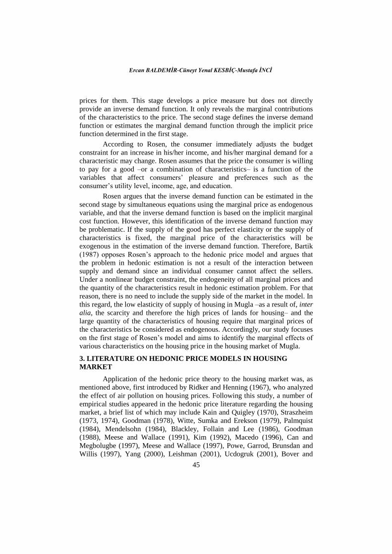
This study estimates the hedonic price model through the E-Views
program. To find out the most suitable model, the study utilizes the most
commonly used top-to-down or general-to-specific approaches (Gujarati 1999)
of Hendry (1985) or the so-called London School of Economics (LSE)
Approach. The initial model covered all of the variables, and then the most
insignificant ones were removed from the model in order until a significance
level of 20.0 was achieved, with the following variables: heating by stove;
living room floor–stone tile; bathroom floor–stone tile; wooden window frames;
betony roof; walls–oil paint; house on the corner; house vacant; house with
front side to north; distance to city center-500–1000m. The variables that were
found to be significant and the related models are presented in Table 2. The
existence of heteroskedasticity in the models was tested via Breusch-Pagan-
Godfrey test and rejected at 05.0 .
Table 2: Results for the Linear, Logarithmic, and Log-linear Models
Variables Linear Model Log-linear Model Log-Log Model
Coefficient Significance Coefficient Significance Coefficient Significance
Central Heating
(Apartment) 12.81457 0.0001 0.117066 0.0000 0.124027 0.0000
Living Room Floor:
unfinished hardwood 5.819712 0.1690 - - - -
Living Room Floor:
Ceramic - - -0.102628 0.0471 -0.093858 0.0638
Bathroom Floor Ceramic 5.101686 0.0498 0.051819 0.0133 0.042196 0.0439
On the Street 4.860699 0.0676 0.035469 0.1235 0.035097 0.1178
Satellite TV 6.782905 0.0538 0.070542 0.0133 0.048301 0.0790
Hidrophor Pump 5.275722 0.0741 0.053024 0.0239 0.054837 0.0184
Parking Lot 3.732982 0.2059 - - 0.029643 0.2226
Modular Kitchen 3.550859 0.1859 0.039558 0.0653 0.029484 0.1641
Sunblind 12.72444 0.0096 0.093856 0.0130 0.098895 0.0074
Solar Water Heating 4.272688 0.1716 0.032140 0.1912 0.039805 0.1019
In-Site -11.02580 0.0003 -0.080453 0.0007 -0.078754 0.0010
Garden - - -0.030564 0.1836 -0.037945 0.1168
Fire Exit - - -0.045414 0.1327 - -
Occupied by Tenant -5.529069 0.0951 - - - -
Occupied by Owner -5.081245 0.1115 - - - -
Front Side to South 5.327686 0.0500 0.044006 0.0422 0.038325 0.0724
Front Side to West -5.490518 0.0830 -0.044016 0.0823 -0.042196 0.0871
On the Corner -3.326854 0.1979 - - - -
Distance to City Centre:
1500-2000m 7.787394 0.0269 0.065401 0.0231 0.066403 0.0175
The Number of Bathrooms 14.86537 0.0054 0.063349 0.1352 0.082357 0.0462
The Number of Rooms -4.772347 0.0615 - - -0.106115 0.1115
Meter Square 0.721088 0.0000 0.005275 0.0000 0.691436 0.0000
The Number of Elevators 13.83910 0.0001 0.104916 0.0002 0.097921 0.0003
The Number of Dwellings
in the Building 0.234487 0.1363 0.002469 0.0482 - -
The Age of the Building - - -0.002554 0.1069 -0.016317 0.1736
F Value 28.86337 0.000000 34.92061 0.000000 36.63798 0.000000
R2/Adjusted R2 0.811703 0.783581 0.816463 0.793082 0.823548 0.801070
Ø 0.424913 6.270495 4.94169
2m-1
12.3380 10.1175 10.8108

Ercan BALDEMİR-Cüneyt Yenal KESBİÇ-Mustafa İNCİ
49
5. INTERPRETATION AND SIGNIFICANCE OF THE COEFFICIENTS
Following are the findings from the hedonic model estimated for Mugla
Center:
Central heating in the apartment, rather than a stove, increases the
hedonic price of the house 12.8 unit in the linear model, 11% in the log-
linear model, and 0.12% in the log-log model. Moreover, the coefficient
of the central heating is positive and significant at 1% in all the three
models.
Ceramic tile floor in the bathroom, rather than stone tile, increases the
hedonic price of the house 5.1 unit in the linear model, 5% in the log-
linear model, and 0.04% in the log-log model. The coefficient of the
ceramic tile floor in the bathroom is positive and significant at 5% in all
the three models.
Location on the street increases the hedonic price of the house 4.8 unit
in the linear model, 3% in the log-linear model, and 0.03% in the log-
log model. The coefficient of location on the street is positive in all the
three models but significant only in the linear model at 10%. In the
other models, this variable does not have any affect on the hedonic
price.
Satellite TV increases the hedonic price of the house 6.78 unit in the
linear model, 7% in the log-linear model, and 0.04% in the log-log
model. The coefficient of satellite TV is positive in all the three models
and significant at 5% in the linear model and at 10% in the other
models.
Hydrophor pump increases the hedonic price of the house 5.27 unit in
the linear model, 5% in the log-linear model, and 0.05% in the log-log
model. The coefficient of hydrophor pump is positive in all the three
models and significant at 10% in the linear model and at 5% in the
other models.
Sunblind increases the hedonic price of the house 12.72 unit in the
linear model, 9% in the log-linear model, and 0.09% in the log-log
model. The coefficient of sunblind is positive in all the three models
and significant at 5% in the log-log model and at 1% in the other
models.
The coefficient of location in a site is negative and significant at 1% in
all the three models. This variable decreases the hedonic price of the
house 11 unit in the linear model, 8% in the log-linear model, and
0.07% in the log-log model.
Front side to south, rather than to north, increases the hedonic price of
the house 5.32 unit in the linear model, 4% in the log-linear model, and
0.03% in the log-log model. The coefficient of this variable is positive

Estimating Hedonic Demand Parameters in Real Estate Market: The Case of Mugla
50
in all the three models and significant at 10% in the linear and log-log
models and at 5% in the log-linear model.
Front side to west, rather than to north, increases the hedonic price of
the house 5.49 unit in the linear model, 4% in the log-linear model, and
0.042% in the log-log model. The coefficient of this variable is negative
and significant at 10% in all the three models.
A distance of 1500-2000m to the city center, compared to that of 500-
1000m, increases the hedonic price of the house 7.78 unit in the linear
model, 6% in the log-linear model, and 0.06% in the log-log model.
The coefficient of this variable is positive and significant at 5% in all
the three models.
One-unit increase in the number of bathrooms increases the hedonic
price of the house 14.86 unit in the linear model, and 6% in the log-
linear model. On the other hand, 1% increase in the number of
bathrooms increases the hedonic price 0.08% in the log-log model. The
coefficient of this variable is positive in all the three models and
significant at 1% in the linear model and 5% in the log-log model,
while it is insignificant in the log-linear model.
One-unit increase in the meter square of the house increases its hedonic
price 0.72 unit in the linear model, and 0.5% in the log-linear model.
On the other hand, 1% increase in the meter square of the house
increases its hedonic price 0.06% in the log-log model. The coefficient
of this variable is positive and significant at 1% in all the three models.
One-unit increase in the number of elevators in the building increases
the hedonic price of the house 13.83 unit in the linear model, and 10%
in the log-linear model. On the other hand, 1% increase in the meter
square of the house increases its hedonic price 0.09% in the log-log
model. The coefficient of this variable is positive and significant at 1%
in all the three models.
F values regarding the findings above are significant at 01.0 level.
In addition, 2R values indicate that these variables explain approximately 81%
of the change in the hedonic price of the house.
6. CONCLUSION
The findings revealed by the econometric model in this study on
estimating hedonic price parameters in the real estate market in Mugla province
have met the theoretical and economic expectations. In other words, considering
the structure and features of Mugla, the estimated coefficients are found to be
significant in terms of both the characteristics of housing and its location (its
position, whether it is in-site or not, etc.).
Ercan BALDEMİR-Cüneyt Yenal KESBİÇ-Mustafa İNCİ
51
As expected, the variables that positively affect the housing price have
been found in all linear, logarithmic, and log-linear models to be central
heating, ceramic bathroom floor, location on the street, satellite TV, hydrophor
pump, modular kitchen, sunblind, solar water heating, front side facing south,
1500-2000 meters to the city center, the number of bathrooms, square meter of
housing, and elevator.
The affect of particularly two variables on housing prices needs to be
interpreted taking into account the structure and characteristics of Mugla.
In-Site Location of Housing: The analysis has revealed by all the three
models that in-site location of housing negatively affect the price of housing,
implying that in-site location decreases the price of housing. The reason
underlying this argument may be that housing in Mugla is mostly in cooperative
type, and their prices are relatively lower, which is attributable to the common
opinion that the material and workmanship used in this kind of housing is of
low quality.
Distance to the City Center (1500–2000m): Our findings suggest that
the price of houses is higher if distance to the city center is 1500–2000 meters.
This is mainly because the closer areas, up to an approximate distance of 2 km,
are not allowed for construction in Mugla. That is why such a distance is
considered close to the city center, and in this manner housing tends to become
more expensive as it gets closer to such a distance.
This study has the merit of identifying the factors that may affect the
housing prices in Mugla at present and in the future by means of hedonic
models, providing a data set on the real estate market for both buyers and
sellers.
7. REFERENCES
Bartik, T. J. (1987). ―The Estimation of Demand Parameters in Hedonic Price
Models‖, The Journal Of Political Economy, 95(1): 81-88.
Blackley, D.M., J.R. Follain and H.Lee. (1986). ―An Evaluation of Hedonic
Price Indexes for Thirty Four Large SMSAs‖, AREUEA Journal, 14(2):
179-205.
Bover, O. and P.Velilla. (2002). ―Hedonic House Prices Without
Characteristics: The Case of New Multiunit Housing‖, European
Central Bank Working Paper Series, Working Paper No.117.
Can, A. and I. Megbolugbe. (1997). ―Spatial Dependence and House Price
Index Construction‖, Journal of Real Estate Finance and Economics,
14: 203–222.
Cohen, J. P. and C. C. Coughlin. (2006). ―Airport-Related Noise, Proximity,
and Housing Prices in Atlanta‖, Federal Reserve Bank of St. Louis
Working Paper , Working Paper 060B.

Estimating Hedonic Demand Parameters in Real Estate Market: The Case of Mugla
52
Colwell, P.F. and G. Dilmore. (1999). ―Who Was First? An Examination of an
Early Hedonic Study‖, Land Economics, 75(4): 620-626.
Court, A. T. (1939). Hedonic Price Indexes with Automotive Examples in
Dynamic of Automobile Demand, General Motors, New York.
Cowling, K. and J. Cubbin. (1972). ―Hedonic Price Indexes for United Kingdom
Cars‖, Economic Journal, 82 (September): 963-978.
Filho, C. M. and O. Bin. (2005). ―Estimation of Hedonic Price Functions via
Additive Nonparametric Regression‖, Empirical Economics, 30: 93–
114.
Goodman, A. C. (1978). ―Hedonic Prices, Price Indices, and Housing Markets‖,
Journal of Urban Economics, 5(4): 471-84.
Goodman, A. C. (1988). ―An Econometric Model of Housing Price, Permanent
Income, Tenure Choice, and Housing Demand‖, Journal of Urban
Economics, 23: 327-353.
Goodman, A. C. (1998). ―Andrew Court and the Invention of Hedonic Price
Analyzis‖, Journal of Urban Economics, 44(2): 291-298.
Gujarati, D.N. (1999). Temel Ekonometri, Çev:Ü.Şenesen ve G:G:Şenesen,
Literatür Yayıncılık, İstanbul.
Harsman, B. and J.M. Quigley. (1991). Housing Markets and Housing
Institutions: An International Comparison,. Kluwer Academic Press,
Boston.
Kain, J. F. and J. M. Quigley. (1970). ―Measuring the Value of Housing
Quality‖, Journal Of The American Statistical Association, 65 (330):
532-548.
Kaul, S. (2006). Hedonism and Culture: Impact on Shopper Behaviour, Indian
Institute of Management Publication.
Kim, S. (1992). ―Search, Hedonic Prices and Housing Demand‖, The Review of
Economics and Statistics, 74(3) : 503-508.
Lancaster, K. J. (1966). ―A New Approach to Consumer Theory‖, Journal of
Political Economy, 74: 132-57.
Leishman, C. (2001). ―House Building and Product Differentiation: An Hedonic
Price Approach‖, Journal of Housing and the Built Environment, 16:
131–152.
Li, W., Prud‘Homme M. and Yu K. (2006). Studies in Hedonic Resale Housing
Price Indexe, OECD-IMF Workshop.
Macedo, R. (1996). ―Hedonic Price Models with Spatial Effects: An
Application to the Housing Market of Belo Horizonte, Brazil‖, Revista
Brasileira de Economia, 29(3): 343-365.
Ercan BALDEMİR-Cüneyt Yenal KESBİÇ-Mustafa İNCİ
53
Maurer, R., M. Pitzer and S. Sebastian. (2004). ―Hedonic Price Indices for the
Paris Housing Market‖, Allgemeines Statistisches Archiv, 88: 303-326.
Meese, R. and N. Wallace. (1991). ―Nonparametric Estimation of Dynamic
Hedonic Price Models and the Constructions of Residential Housing
Price Indices‖, AREUEA Journal, 19(3):308-332.
Meese, R. and N. Wallace. (1997). "The Construction of Residential Housing
Price Indices: A Comparison of Repeat-Sales, Hedonic-Regression, and
Hybrid Approaches", Journal of Real Estate Finance and Economics,
14: 51–73.
Mendelsohn, R. (1984). ―Estimating the Structural Equations of Implicit
Markets and Household Production Functions‖, The Review of
Economics and Statistics, 66(4): 673-677.
Ogwang, T. and B. Wang. (2002). ―A Hedonic Price Function for a Northern
BC Community‖, Social Indicators Research, 61: 285-296.
Palmquist, R. B. (1984). ―Estimating the Demand for the Characteristics of
Housing‖, Review of Economics and Statistics, 66(3): 394-404.
Powe, N.A., Garrod G.D., Brunsdon C.F. and K.G. Willis. (1997). ―Using a
Geographic Information System to Estimate a Hedonic Price Model of
the Benefits of Woodland Access‖, Forestry, 70(21): 39-149.
Ramanathan, R. (1998). Introductory Econometrics with Applications, The
Dryden Press, Fourth Edition.
Ridker, R.G. and J.A. Henning. (1967). ―The Determinants of Residential
Property Values with Special Reference to Air Pollution‖ The Review of
Economics and Statistics, 49: 246–257.
Rosen, S. (1974). ―Hedonic Prices and Implicit Markets: Product
Differentiation in Pure Competition‖, Journal of Political Economy, 82:
34-55.
Straszheim, M.R. (1973). ―Estimation Of The Demand For Urban Housing
Services From Household Interview Data‖, Review of Economics and
Statistics, 55: 1-8.
Straszheim, M.R. (1974). ―Hedonic Estimation of Housing Market Prices: A
Further Comment‖, The Review of Economics and Statistics, 56(3):
404-406.
Toda, Y. and N. N. Nozdrina. (2004). ―The Spatial Distribution of the
Apartment Prices In Moscow in 2002: Hedonic Estimation from Micro
Data‖ ENHR Conference July 2nd-6th 2004, Cambridge.
Üçdoğruk, Ş. (2001). ―İzmir İlinde Emlak Fiyatlarına Etki Eden Faktörler:
Hedonik Yaklaşım‖, D.E.Ü. İ.İ.B.F. Dergisi, 16(2): 149-161.
Wallace, H.A. (1926). ―Comparative Farmland Values in Iowa‖, Journal of
Land and Public Utility Economics, 2: 385-392.

Estimating Hedonic Demand Parameters in Real Estate Market: The Case of Mugla
54
Wen H., J. Sheng-Hua and G. Xiao-Yu. (2005). ―Hedonic Price Analysis of
Urban Housing: An Empirical Research on Hangzhou, China‖, Journal
of Zhejiang University Science, 6A (8):907-914.
Wen, H.Z., J.F. Lu, and L. Lin. (2004). An Improved Method of Real Estate
Evaluation Based on Hedonic Price Model, International Management
Conference.
Wilhelmsson, M. (2002). ―Household Expenditure Patterns for Housing
Attributes: A Linear Expenditure System with Hedonic Prices‖, Journal
of Housing Economics, 11: 75–93.
Witte, A. D., H. Sumka and J. Erekson. (1979). ―An Estimate of a Structural
Hedonic Price Model of the Housing Market: An Application of
Rosen's Theory of Implicit Markets‖, Econometrica, 47: 1151-72.
Yang, Z. (2000). ―An Application of the Hedonic Price Model with Uncertain
Attribute: The Case of the People's Republic of China‖, Property
Management, 19(1): 50-63.
Yankaya, U. ve M. Çelik. (20059. ―İzmir Metrosunun Konut Fiyatları
Üzerindeki Etkilerinin Hedonik Fiyat Yöntemi İle Modellenmesi‖,
D.E.Ü. İ.İ.B.F. Dergisi, 20(2): 61-79

Ercan BALDEMİR-Cüneyt Yenal KESBİÇ-Mustafa İNCİ
55
Appendix: Examples of Hedonic Pricing Models in House Markets
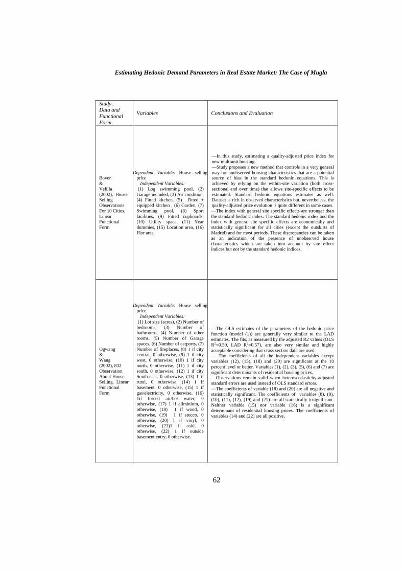
Study,
Data and Functional
Form
Variables Conclusions and Evaluation
Ridker
&
Henning
(1967) , 167
Observation
About House
Selling, Linear
Functional
Form
Dependent Variable: Median value
of owner-occupied single family
housing units
Independent Variables:
(1) An index of annual geometric
mean sulfation levels, (2) Median
number of rooms per housing unit,
(3) Percentage recently built, (4)
Total houses per square mile of
tracts, (5) Time zone for central
business district, (6) Percentage non-
white housing units, (7) School
quality, (8) Occupation ratio, (9)
Highway accessibility, (10) İllionis/
Missouri dummy variable, (11)
Persons per unit, (12) Median family
income, (13) Index of annual
geometric mean concentrations of
suspended particulates gathered by
high-volume air samplers, (14)
Percentage substandart, (15) Crime
rate, (16) Shopping area accessibility,
(17) Industrial area accessibility, (18)
Social area analysis indexes.
—This study was one of the earliest to apply hedonic price
theory for analyze the housing market and calculated the
impact of improving environmental quality on housing
price.
—The variables which causes multicollinearity problem
also featured in the study and introduced the results if
including these varibles or not. Thus, adjustments for
multicollinearity choosing four different estimating
method.
—The most important results are statistically significant
and all are fairly reasonable within the context of the area.
—Sulfation levels to which any single-family dwelling
unit is exposed were to drop by 0.25 mg./100cm2/day, the
value of that property could be expected to rise by at least
$83 and more likely closer to $245.23.
—Characteristics specific to the property [variable (2),(3)
and (4)] all turned out to be important explanatory
variables. The sign and magnitudes of their coefficients are
as expected.
— Both variables (5) and (9) are statistically significant.
The coefficients attached to variable (5) , however, are not
quite as expected.
—Variable (8) proved to be best estimated among
neighbourhood characteristics. The coefficients of variable
(7) are positive.
Kain
&
Quigley
(1970) , 1184
Observation In
The Entire
Model And
854
Observation
For The
Restricted
Model
About House
Selling,,Semi-
Logarithmic
and Linear
Functional
Forms
Dependent Variable: Dwelling unit
price
Independent Variables:
(1) Basic residential quality, (2)
Dwelling unit quality, (3) Quality of
proximate properties, (4)
Nonresidential usage, (5) Avarage
structure quality, (6) Proportion
white in census tract, (7) Median
schooling of adults in census tract,
(8) Public School achievement, (9)
Number of major crimes, (10) Age of
structure, (11) Number of rooms
(natural log.), (12) Number of
bathrooms, (13) Parcel area
(hundreds of sq. ft.), (14) First flor
area (hundreds of sq. ft.), (15) Single
detached, (16) Duplex, (17) Row,
(18) Apartment, (19) Rooming
house, (20) Flat, (21) No heat
included in rent, (22) No water
included in rent, (23) No major
appliances included in rent, (24) No
furniture included in rent, (25) Hot
water, (26) Central heat, (27)
Duration of occupancy (years), (28)
Owner in building
—This article estimates the market value, or the implicit
prices of specific aspects of the bundles of residential
services consumed by urban households. Quantitative
estimates were obtained by regressing market price of
owner-and renter-occupied dwelling units on measures of
the qualitative and quantitative dimensions of the housing
bundles.
—The measures of residential quality obtained by using
factor analysis to aggregate some 39 indexes of the quality.
—For renters equations used 25 variable and for owners
equations used 15 variable in the study.
—The analysis indicates that the quality of the bundles of
residential services has about as much effect on the price
of housing as such objective aspects as the number of
rooms, number of bathrooms, and lot size.
—For renters, among the first 5 quality variables, variable
(1), (2) and (5) are statistically significiant in the model
which have restristed observation. For owners, among the
first 5 quality variables, variable (3) and (5) are not
statistically significiant in the model which have restristed
observation. For renters equations only 16 variable and for
owners equations only 5 variable are statistically
significiant at %5 significance level.
—The most striking difference when the model is
reestimated for the entire obvervations is the increase in
the significance of the coefficients.

Estimating Hedonic Demand Parameters in Real Estate Market: The Case of Mugla
56
Study,
Data and Functional Form
Variables Conclusions and Evaluation
Straszheim
(1973), Household
Interview Data For
1965
(100-200
Observation About
House Selling),
Linear Functional
Form
Dependent Variable: Price of
standartized dwelling unit
Independent Variables:
(1) Probability of ownership, (2)
Number of rooms in dwelling
units, (3) Structure age dummies,
(4) Lot size dummies, (5)
Structure condition dummies, (6)
Unsound condition dummies, (7)
Sample size
—Separate equations were estimated for owner and rental
units, and for each geographic submarket.
—It was found strong relationship between house price
and variables (3), (4) and (7).
— Variables (3) and (4) were always statistically
significiant.
—Analysis of covariance tests reveal satatistically
significiant differences in the equations across zones.
—There is substantial spatial variation in the price of most
attributes of housing services.
Straszheim
(1974), Pooled
Data Of The 3
Different District
About House
Characteristics,
Linear Functional
Form
Dependent Variable: House
selling price
Independent Variables:
(1) Number of rooms, (2) Built in
pre1940, (3) Built in 1940–1945,
(4) Built in 1950–1959, (5) Lot
size less than 2 acre, (6) Lot size
between 3–5 acre, (7) Lot size
greater than 5 acre, (8) Unsound
condition dummy , (9) Sample
size
—F-tests reveal that the geographic stratification reduces
the residual sum of squared errors. A few of the individual
submarket equations are presented to illustrate the range of
estimates obtained.
—Though suburban submarkets exhibit more price
homogeneity, there are also limits to how wide a
geographic area can be employed.
—The discussion of hedonic price estimation might more
usefully be directed to the criteria which should be
employed to define homogenous submarkets within urban
areas.
Goodman
(1978), 1835
Observation About
House Selling,
Box-Cox
Functional Form
Dependent Variable: House
selling price
Independent Variables:
(1) Lot size in sq. ft., (2) 1 if house
is all brick; 0 otherwise, (3) 1 if
hardwood floors; o otherwise, (4)
Number of covered garage spaces,
(5) Age of house in years, (6)
Number of rooms excluding
bathrooms, lavatories, (7) Number
of full bathrooms, (8) Number of
Lavatories, (9) Indoor living space
in sq. Ft., (10) Number of
fireplaces, (11) Percentage balack
population, (12) Percentage
families with income less than
5000 $, (13) Percentage of
population over age 25 with 13 or
more years of education, (14) 1 if
black is greater than %5 and less
than %15, (15) Principle
components measure of
neighbourhood attitudes
— This study appears to clarify several aspects of housing
analysis using hedonic prices, with respect to market
segmentation, functional form and behavior of prices
within submarkets. In positing various spatially and
temporally separate submarkets, covariance analysis
indicates heterogeneity of coefficients.
-—Model results showed that, Variables affect the house
prices differently in urban and suburb areas and for both
structure and neighbourhood characteristics the price are
up to 20% higher than the suburbs.
— Intrametropolitan examination of structural and
neighborhood quality reveals that the relative valuation of
physical improvements in housing is smaller in the central
city than in the suburbs, while the relative valuation of
improved neighborhoods is relatively constant.
-— Aggregation of hedonic price coefficients into
standardized units yields significantly higher housing
prices in the central city than in its suburbs, as well as
differential effects of structural and neighborhood
improvements among submarkets.

Ercan BALDEMİR-Cüneyt Yenal KESBİÇ-Mustafa İNCİ
57
Study,
Data and
Functional Form
Variables Conclusions and
Evaluation
Witte
&
Sumka
&
Erekson
(1979), 500
Observation
About House
Rents In Four
City, Linear
Functional Form
Dependent Variable: House rent
Independent Variable (For Consumers): (1) Total annual current
income of household, (2) Age in years of the head of household, (3)
1 If the head of household is employed in blue collar job; 0
otherwise, (4) 1 If the head of household is employed in white collar
job; 0 otherwise, (5) 1 if the highest level of education attained by
head of household is high school; 0 otherwise, (6) 1 if the head of
household has education beyond the high school level; 0 otherwise,
(7) The number of persons in the household, (8) 1 if the household
head is female and 0 if male.
Independent Variable (For Supplier): (1) The number of years the
landlord has owned the dwelling, (2) 1 if there is a lease; 0
otherwise, (3) 1 if the family has lived in the dwelling for five years
or more; 0 otherwise, (4) 1 if the landlord is resident in the dwelling;
0 otherwise, (5) 1 if rent is collected more often than once a month;
0 otherwise, (6) 1 if a professional manager is employed; 0
otherwise, (7) The number of rental units owned, (8) 1 if ownership
is of the corporate form; 0 otherwise, (9) 1 if the rental housing
owned was acquired by inheritance; 0 otherwise, (10) 1 if the head
of household is black; 0 otherwise.
Other Independent Variables: (1) Dwelling quality, (2) Dwelling
size, (3) Lot size, (4) Neighbourhood quality, (5) A measure of
accessibility
—In this study, estimated a
simultaneous system of hedonic
price equations suggested by the
work of Rosen. This system
consisted of bid and offer curves
for each of housing bundle
attributes, dwelling quality,
dwelling size, and lot size.
—Empirical results confirm the
theoretically expected negative
coefficient for each attribute in
its own bid price equation and
the expected positive or zero
coefficient for each attribute in
its own offer function.
—An examination of cross
price relationships among the
attributes revealed an intriguing
and generally logical pattern of
interactions both on the demand
and the supply sides.
Palmquist
(1984),
.20297
Observation
About House
Selling,
Linear,
Semi-
Logarithmic,
Log-Linear
and Inverse
Semi-
Logarithmic
Functional
Forms
Dependent Variable: House selling price
Independent Variables:(1) Area of lot in sq. ft., (2) Finished interior
area in sq. ft., (3) Finished interior area squared, (4) Number of
bathrooms, (5) Year of construction, (6) Number of stalls in garage,
(7) Number of stalls in carport, (8) 1 if garage is detached from
house, (9) 1 if there is underground wiring, (10) 1 if there is a
dishwasher, (11) 1 if there is a garbage disposal, (12) 1 if there is
central air conditioning, (13) 1 if there is wall air conditioning units,
(14) 1 if there is a ceiling fan, (15) 1 if the date of sale was 1976,
(16) Excellent condition, (17) Fair condition, (18) Poor condition,
(19) Brick or stone exterior finish, (20) 1 if there is a full basement,
(21) 1 if there is a partial besement, (22) 1 if there are one or more
fireplaces, (23) 1 if there is a swimming pool, (24) The annual
arithmetic mean of the particulate air pollution level, (25) The
median age of the residents of the census tract, (26) The median
family income of residents of the census tract, (27) The percentage
of workers in the census tract that has a blue collar job, (28) The
percentage of houses in the census tract that has changed ownership
within the last five years, (29) The percentage of the population of
the census tract that is classified as non-white, (30) The percentage
of the population of the census tract over 24 years old that has
graduated from high school, (31) The percentage of the structures in
the census tract with 1.00 or less persons per room, (32) The number
of work destinations within the census tract divided by the area of
the census tract, (33) Adjusted monthly housing expenditure, (34)
Hedonic price of sq. ft. of living space, (35) Hedonic price of
bathrooms, (36) Hedonic price of the percentage of the census tract
with high school degrees, (37) Hedonic price of racial homogeneity,
(38) Hedonic price of lot area, (39) Hedonic price of reduction in
age of house, (40) Age of the purchaser, (41) 1 if the purchaser is
single, (42) Number of dependents in the family making the
purchase, (43) 1 if the purchaser is black.
—First, linear hedonic
regression equations were
constructed and in the second
srtage estimated logarithmic
linear estimates for house
characteristics in the study. To
reduce the costs of estimation,
the search was restricted to the
four functional forms most
frequently used: linear, semi-
logarithmic, log-linear and
ınverse semi-logarithmic.
—With approximately 200
coefficients estimated, there are
only 17 with incorrect signs and
none of these are for the most
important variables. Hedonic
regression results showed that
variables (3), (8), (18), (24), (28)
and (29) affects house prices
negatively. First 32 variables
except variables (3), (8), (18),
(24), (28) and (29) affects house
prices positively and the
variables which were positively
affects house prices have
expected signs and magnitudes,
also they were statistically
significiant. In the second stage,
variables (33), (34) (42) and (43)
were more effective on the house
prices and these variables which
were statistically significiant
have positive coefficients.
Estimating Hedonic Demand Parameters in Real Estate Market: The Case of Mugla
58
Study,
Data and
Functional Form
Variables Conclusions and Evaluation
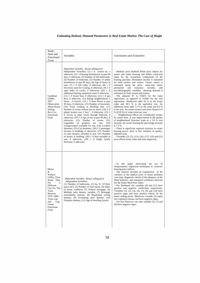
Goodman
(1988),
2857
Observation
About House
Selling,
Box-Cox
Functional
Form
Dependent Variable: House selling price
Independent Variables: (1) 1 if central air, o
otherwise, (2) 1 if heating breakdowns in past 90
days, 0 otherwise, (3) Number of full bathrooms,
(4) Number of bedrooms, (5) Number of utility
breakdowns in past 90 days, (6) Age of house in
year, (7) 1 if full cellar, 0 otherwise, (8) 1 if
electricity used for cooking, 0 otherwise, (9) 1 if
open holes or cracks, 0 otherwise, (10) 1 if
additional heating equipment used, 0 otherwise ,
(11) 1 if Steam heat, 0 otherwise, (12) 1 if gas
heat, 0 otherwise, (13) Rating neighborhood, 1
(best)…,4 (worst), (14) 1 if fuses blown in past
90 days, 0 otherwise, (15) Number of lavatories,
(16) Years residing in dwelling unit, (17)
Number of rooms without hot air ducts, (18) 1 if
plaster broken over 1 foot 2 , 0 otherwise, (19) 1
if Access to other rooms through bedroom, 0
otherwise, (20) 1 if sign of rats ın past 90 days, 0
otherwise, (21) Number of rooms, (22)
Logarithm of property tax rate, (23)
Garage/carport available for use, (24) Location
dummies, (25) City dummies, (26) 1 if passenger
elevator in building, 0 otherwise, (27) Number
of extra features included in rent, (27) Number
of stories in building, (28) 1 if heat included in
rent, 0 otherwise, (29) 1 if Single family
Structure, 0 otherwise.
—Hedonic price methods define price indices for
owner and renter housing and define value-rent
ratios for the investment components of the
housing purchase. Permanent income is estimated
for both owners and renters. Tenure choice is
estimated using the price, value-rent ratios,
permanent and transitory incomes, and
sociodemographic variables. Housing demand is
estimated for both owners and renters.
—The adjusted R2 is 0.6025 for the value
regressions, as opposed to 0.4585 for the rent
regressions. Abathroom adds 26 % to the house
value and 28.5 % to the apartment rent. An
additional room adds 7.3 % to the value and 6.0 %
to the rent. An owner (renter) unit loses About 0.53
% (0.28 %) of value (rent) per year.
— Neighborhood effects are considerably weaker
for renter units. A unit improvement in the quality
of neighborhood Structure leads to a 3.8 % rent
increase; for owner housing the percentage increase
is 7.5 %.
—There is significant regional variation in owner
housing prices, there is less variation in quality-
adjusted rents.
—Variables (2), (5), (13), (16), (17), (19) and (22)
were affects house value and rents negatively.
Meese
&
Wallace
(1991), Time
Series Data
For 2
Different
City For The
Years
Between
1970–1988,
Trans-Log
and Log-
Linear
Functional
Form
Dependent Variable: House selling price
Independent Variables:
(1) Number of bathrooms, (2) Sq. Ft. Of floor
space (m2), (3) Number of total rooms, (4) Index
of house condition, (5) Federal mortgage, (6)
Multiple sales dummy variable, (7) Mortgage
assumability dummy, (8) Residential zoning
dummy, (9) Swimming pool dummy, (10)
Fireplace dummy, (11) Age of dwelling (years).
—In this paper advocating the use of
nonparametric regression techniques to construct
housing price indices.
—The analysis includes an examination of the
variation in the implicit price of house attributes
over time, diagnostic checks of the adequacy of the
fitted hedonics, and simulated confidence intervals
for the Fisher Ideal Price index.
—For Diedmont city variables (6) and (11) have
positive and negative coefficients respectively.
Variables (1), (2), (3), (4), (7), (9) and (10) have
positive signs and have positive effects on the
house selling prices. Moreover, variable (5) states
less expensive houses and have negative signs.
—For San Francisco city only variable (5), (7) and
(8) have negative signs.

Ercan BALDEMİR-Cüneyt Yenal KESBİÇ-Mustafa İNCİ
59
Study,
Functional Form, Data
Variables Conclusions and Evaluation
Can
&
Megbolugbe
(1997), 944
Observation
About House
Selling, Linear
Functional
Form
Dependent Variable: House selling
price
(1) Living area in sq. ft., (2)
Land area in sq. ft., (3) Age of
the structure, (4) Composite
neighborhood quality score
Neighborhood quality variables:
—Owner-occupancy rate
—Median household income
—Percentage of residents with
college education
—Percentage of households
paying at least 30 % of income
on monthly housing costs
—Median value of owner-
occupied housing
—Vacancy rate
—Median age of housing stock
—Percentage of detached signle-
family units
—Percentage of white-headed, balack-
headed and hispanic-headed
—Study illustrates the importance of spatial dependence
in both the specification and estimation of hedonic price
models. In this article, presenting the importance of
spatial dependence on the specification of a house price
function due to the presence of spatial spillover effects
in the operation of local housing markets. With the
spatial models which constructed in the article, it would
be possible to adjust the confidence intervals of the
metropolitan –level indices to reflact the localized
dependencies in the house price determination process.
—Models also achieve very reasonable estimates of
marginal prices for selected attributes. Spatial
dependence plays an important role in the house price
determination process.
— Variable (2) is not statistically significant in both 6
regression equations of study. Except variable (2), other
variables have a hidh significance levels and have
different effects on the house selling prices.
—This study rpresents an attempt to derive useful house
price indices from large data sets containing only
alimited number of variables.
- —The R2 value in the spatial hedonic expansion models
which have strong consequences was more than spatial
hedonic and traditional hedonic models.
Meese
&
Wallace
(1997), 27606
Observation
About House
Selling In Two
District Over
An 18 Years
Period,
Translog and
Log-Linear
Functional
Forms
Dependent Variable: House selling
price
Independent Variables:
(1) Number of bathrooms, (2) Number
of bedrooms, (3) Sq. ft. of lot size, (4)
Number of rooms, (5) House quality
index, (6) Age of structure.
—This article examines a number of hypotheses that
underpin the repeat-sales and hedonic approaches to the
construction of housing price indices, as well as the
practical problems associated with the implementation
od either approach.
—Study examines a hybrid procedure that combines
elements of both the repeat-sales and hedonic regression
techniques.
—In this article, documenting the shortcomings of
repeat-sales price indices when they are constructed on
municipality-level data sets. The indices suffer from
sample selection bias and nonconstancy of implicit
housing characteristic prices, and the yare quite sensitive
to small sample problems.
—The standart variance specification of repeat-sales
approaches appears to be inappropriate for data at the
municipality level.
—Repeat sales methods reject the assumption that
changing attribute prices over time.
Estimating Hedonic Demand Parameters in Real Estate Market: The Case of Mugla
60
Study,
Data and Functional
Form
Variables Conclusions and Evaluation
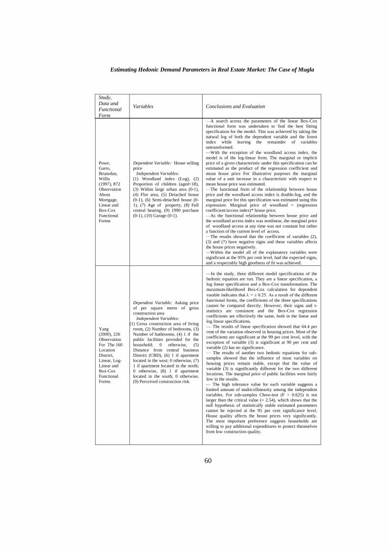
Powe,
Garro,
Brunsdan,
Willis
(1997), 872
Observation
About
Mortgage,
Linear and
Box-Cox
Functional
Forms
Dependent Variable: House selling
price
Independent Variables:
(1) Woodland index (Log), (2)
Proportion of children (aged<18),
(3) Within large urban area (0-1),
(4) Flor area, (5) Detached house
(0-1), (6) Semi-detached house (0-
1), (7) Age of property, (8) Full
central heating, (9) 1990 purchase
(0-1), (10) Garage (0-1).
—A search across the parameters of the linear Box-Cox
functional form was undertaken to find the best fitting
specification for the model. This was achieved by taking the
natural log of both the dependent variable and the forest
index while leaving the remainder of variables
untransformed.
—With the exception of the woodland access index, the
model is of the log-linear form. The marginal or implicit
price of a given characteristic under this specification can be
estimated as the product of the regression coefficient and
mean house price For illustrative purposes the marginal
value of a unit increase in a characteristic with respect to
mean house price was estimated.
—The functional form of the relationship between house
price and the woodland access index is double-log, and the
marginal price for this specification was estimated using this
expression: Marginal price of woodland = (regression
coefficient/access index)* house price.
—As the functional relationship between house price and
the woodland access index was nonlinear, the marginal price
of woodland access at any time was not constant but rather
a function of the current level of access.
—The results showed that the coefficient of variables (2),
(3) and (7) have negative signs and these variables affects
the house prices negatively.
—Within the model all of the explanatory variables were
significant at the 95% per cent level, had the expected signs,
and a respectably high goodness of fit was achieved.
Yang
(2000), 226
Observation
For The 160
Location
District,
Linear, Log-
Linear and
Box-Cox
Functional
Forms
Dependent Variable: Asking price
of per square metre of gross
construction area
Independent Variables:
(1) Gross construction area of living
room, (2) Number of bedrooms, (3)
Number of bathrooms, (4) 1 if the
public facilities provided for the
household; 0 otherwise, (5)
Distance from central business
District (CBD), (6) 1 if apartment
located in the west; 0 otherwise, (7)
1 if apartment located in the north;
0 otherwise, (8) 1 if apartment
located in the south; 0 otherwise,
(9) Perceived construction risk.
—In the study, three different model specifications of the
hedonic equation are run. They are a linear specification, a
log linear specification and a Box-Cox transformation. The
maximum-likelihood Box-Cox calculation for dependent
varable indicates that = ± 0.25. As a result of the different
functional forms, the coefficients of the three specifications
cannot be compared directly. However, their signs and t-
statistics are consistent and the Box-Cox regression
coefficients are effectively the same, both in the linear and
log linear specifications.
— The results of linear specification showed that 64.4 per
cent of the variation observed in housing prices. Most of the
coefficients are significant at the 99 per cent level, with the
exception of variable (3) is significant at 90 per cent and
variable (2) has no significance.
— The results of another two hedonic equations for sub-
samples showed that the influence of most variables on
housing prices remain stable, except that the value of
variable (3) is significantly different for the two different
locations. The marginal price of public facilities were fairly
low in the results.
— The high tolerance value for each variable suggests a
limited amount of multicollinearity among the independent
variables. For sub-samples Chow-test (F = 0.625) is not
larger than the critical value (= 2.54), which shows that the
null hypothesis of statistically stable estimated parameters
cannot be rejected at the 95 per cent significance level.
House quality affects the house prices very significantly.
The most important preference suggests households are
willing to pay additional expenditures to protect themselves
from low construction quality.
Ercan BALDEMİR-Cüneyt Yenal KESBİÇ-Mustafa İNCİ
61
Study,
Data and
Functional Form
Variables Conclusions and Evaluation
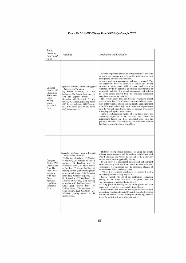
Leishman
(2001), 1155
Observation
About New
House
Selling,
Linear
Functional
Form
Dependent Variable: House selling price
Independent Variables:
(1) Second bedroom, (2) Third
bedroom, (3) Fourth bedroom, (4)
Flor are (square meters) (5)
Bungalow, (6) Detached, (7) Mid
terrace, (8) Garage, (9) Dining room,
(10) Second bathroom, (11) En-suite,
(12) Box room, (13) Utility room,
(14) Year dummies.
—Hedonic regression models are constructed and Chow tests
are performed in order to test the null hypothesis of product
homogeneity between house builders.
— In the study two regression model was constructed. The
first regression model is intended to explain and predict
variation in house prices within a given local area with
reference only to the attributes or physical characteristics of
houses sold and time. The second regression model includes
the factor scores derived from the principal component
analysis as explanatory variables.
—The results show that the hedonic regression model
explains more than 83% of the total variation in house prices.
Most of the variables entered into the equation are significant
at the 99% level and the majority of the estimated parameters
have the ‗correct‘ sign, that is, they are positive or negative
in keeping with a priori expectations.
—In the second regression model, 12 of the factor scores are
statistically significant at the 1% level. The statistically
insignificant factors are those associated only with the
quarterly dummies. The collinearity statistics now indicate
that there is no multicollinearity problem.
Üçdoğruk
(2001), 2718
Observations
From The
Face To Face
Interview
With Real
Estate
Agencies,
Log-Linear
Functional
Form
Dependent Variable: House selling price
Independent Variables:
(1) Number of balkony, (2) Number
of elevator, (3) Number of flats in
aparment, (4) Dwelling size, (5)
Number of rooms, (6) Floor number
of dwelling, (7) Age of dwelling, (8)
Heating system, (9) Furnishing status
of room and saloon, (10) Bathroom
floor, (11) Window carpentry, (12)
Roof proofing, (13) Wallboard, (14)
Location of dwelling, (15) Building
of kitchen, (16) Satellite system, (17)
Cable, (18) Pressure tank, (19)
Parking place, (20) Venetian, (21)
Solar energy, (22) Caretaker, (23)
Whether housing located at the
garden or site.
—Hedonic Pricing model estimated by using the simple
ordinary least squares method, for the best model choice used
Wald-F statistics and ―from the general to the particular‖
approach which was suggested byHendry.
—In this study, it is established both general and restricted
model and study with restricted model is more available.
Furthermore, it is mentioned that the percentage changes of
each variables affects the house prices.
— When it is examined conclusions of restricted model,
variable (5) was statistically significant.
—Except variable (5), all of the coefficients estimation
belong to the other variables correspond theoritical
expectations and is statistically significant.
—Taking place the housing in site, in the garden and with
solar energy resulted as economically insignificant.
—İmprovements that occurs in housing characteristics have
been raising housing prices at different degrees; both housing
features and external factors (floorspace of housing, whether
it is in the site) significantly affects the price.
Estimating Hedonic Demand Parameters in Real Estate Market: The Case of Mugla
62
Study,
Data and
Functional Form
Variables Conclusions and Evaluation
Bover
&
Velilla
(2002), House
Selling
Observations
For 10 Cities,
Linear
Functional
Form
Dependent Variable: House selling
price
Independent Variables:
(1) Log swimming pool, (2)
Garage included, (3) Air condition,
(4) Fitted kitchen, (5) Fitted +
equipped kitchen , (6) Garden, (7)
Swimming pool, (8) Sport
facilities, (9) Fitted cupboards,
(10) Utility space, (11) Year
dummies, (15) Location area, (16)
Flor area
—In this study, estimating a quality-adjusted price index for
new multiunit housing.
—Study proposes a new method that controls in a very general
way for unobserved housing characteristics that are a potential
source of bias in the standard hedonic equations. This is
achieved by relying on the within-site variation (both cross-
sectional and over time) that allows site-specific effects to be
estimated. Standard hedonic equations estimates as well.
Dataset is rich in observed characteristics but, nevertheless, the
quality-adjusted price evolution is quite different in some cases.
—The index with general site specific effects are stronger than
the standard hedonic index. The standard hedonic index and the
index with general site specific effects are economically and
statistically significant for all cities (except the outskirts of
Madrid) and for most periods. These discrepancies can be taken
as an indication of the presence of unobserved house
characteristics which are taken into account by site effect
indices but not by the standard hedonic indices.
Ogwang
&
Wang
(2002), 832
Observation
About House
Selling, Linear
Functional
Form
Dependent Variable: House selling
price
Independent Variables:
(1) Lot size (acres), (2) Number of
bedrooms, (3) Number of
bathrooms, (4) Number of other
rooms, (5) Number of Garage
spaces, (6) Number of carports, (7)
Number of fireplaces, (8) 1 if city
central, 0 otherwise, (9) 1 if city
west, 0 otherwise, (10) 1 if city
north, 0 otherwise, (11) 1 if city
south, 0 otherwise, (12) 1 if city
South-east, 0 otherwise, (13) 1 if
rural, 0 otherwise, (14) 1 if
basement, 0 otherwise, (15) 1 if
gas/electricity, 0 otherwise, (16)
1if forced air/hot water, 0
otherwise, (17) 1 if aliminium, 0
otherwise, (18) 1 if wood, 0
otherwise, (19) 1 if stucco, 0
otherwise, (20) 1 if vinyl, 0
otherwise, (21)1 if osid, 0
otherwise, (22) 1 if outside
basement entry, 0 otherwise.
—The OLS estimates of the parameters of the hedonic price
function (model (1)) are generally very similar to the LAD
estimates. The fits, as measured by the adjusted R2 values (OLS
R2=0.59, LAD R2=0.57), are also very similar and highly
acceptable considering that cross section data are used.
— The coefficients of all the independent variables except
variables (12), (15), (18) and (20) are significant at the 10
percent level or better. Variables (1), (2), (3), (5), (6) and (7) are
significant determinants of residential housing prices.
—Observations remain valid when heteroscedasticity-adjusted
standard errors are used instead of OLS standard errors.
—The coefficients of variable (18) and (20) are all negative and
statistically significant. The coefficients of variables (8), (9),
(10), (11), (12), (19) and (21) are all statistically insignificant.
Neither variable (15) nor variable (16) is a significant
determinant of residential housing prices. The coefficients of
variables (14) and (22) are all positive.

Ercan BALDEMİR-Cüneyt Yenal KESBİÇ-Mustafa İNCİ
63
Study,
Data and
Functional Form
Variables Conclusions and Evaluation
Wilhemsson
(2002), Cross-
Sectional Data
Thet Include
Only 318
Transactions,
Box-Cox and
Log-Linear
Functional
Forms
Dependent Variable: House selling
price
Independent Variables:
(1) Living area (Price), (2) Lot
size (Price), (3) Quality (Price), (4)
Quietness (Price), (5) Changes in
real economics, (6) Permanent
income, (7) Mortgage, (8) Family
size, (9) Household age.
— The main objective of this paper is to demonstrate how the
linear expenditure system approach can be used in the
estimation of housing attribute elasticities.
—Estimation of the hedonic price equation is conducted using
a Box–Cox transformation. Study have chosen to use four
specifications of the hedonic price equation that together will
provide four estimates of the implicit price. Model 1, the base
specification, is a log-linear specification using the whole
sample period; Model 2 is a Box–Cox specification using the
whole sample; Models 3 and 4 are based on a different
transformation of the hedonic price equation in each time
period.
—The implicit prices were estimated by a Box–Cox
transformed hedonic price equation. However, the robustness
or sensitivity of the estimates in the linear expenditure system
was tested for different choices of specifications; the
conclusion was reached that they are relatively insensitive to
functional form.
All the estimated parameters differ statistically significantly
from zero and have the expected sign. Furthermore, each is of
reasonable magnitude. An increase by 1% of the living-area
attribute will increase the price of the house by 0.5%. The five
variables can explain around 60% of the deflated price
variation.
Toda&
Nozdrina
(2004) , 5282
Observation
About House
Selling
(February
2002) and
6551
Observation
About House
Selling
(April 2002),
Linear
Functional
Form
Dependent Variable: House selling
price
Independent Variables:
(1) Size of an apartment including
a bathroom and hallway, (2) The
size of a kitchen, (3) The distance
from a nearby metro station is
measured in meters, (4) The
distance from the city center, (5)
Location, (6) Wage arrears, (7) 2
room, (8) 3 room, (9) 4 and more
rooms, (10) Aroom can be
accessed dirctly from a hallway or
not (11) The material for he
exterior wall, (12) The number of
balkony, (13) Elevator, (14) The
materials for floor, (15) Apartment
repaired or not, (16) Location
condition, (17) East, (18)
Northeast, (19) Northwest, (20)
West, (21) Southwest, (22) South,
(23) Southeast with North as the
base, (24) The number of workers
the enterprises want to employ,
(25) Apartment new, (26)
Apartment under construction
—The data used in these estimations are the various attributes
of individual apartments and the prices proposed by the
agents who were selling them in February and April 2002. All
regression equations for two period were estimated by
ordinary least squares method and obtained the same results
for each one.
—The result of the estimation of regression equation on the
data in February 2002 is in the following. Number of
observations is 5,282. The F-ratio with the degrees of
freedom 22 and 5259 is equal to 256.58. The R-squared and
the adjusted R-squared are equal to 0.5177, 0.5157,
respectively.
—The result of the estimation of regression equation on the
data in April 2002 is in the following. Number of
observations is 6,551. The F-ratio with the degrees of
freedom 21 and 6529 is equal to 326.24. The R-squared and
the adjusted R-squared are equal to 0.5120, 0.5105,
respectively.
— Among the attributes of an apartment, the total size, the
size of kitchen, the number of room, the degree of certainty
with which a buyer can move into an apartment in a short
period play a significant role. The building materials for wall
and for floor, whether an apartment has been repaired,
whether the building has an elevator are also relevant in the
determination of apartment price.
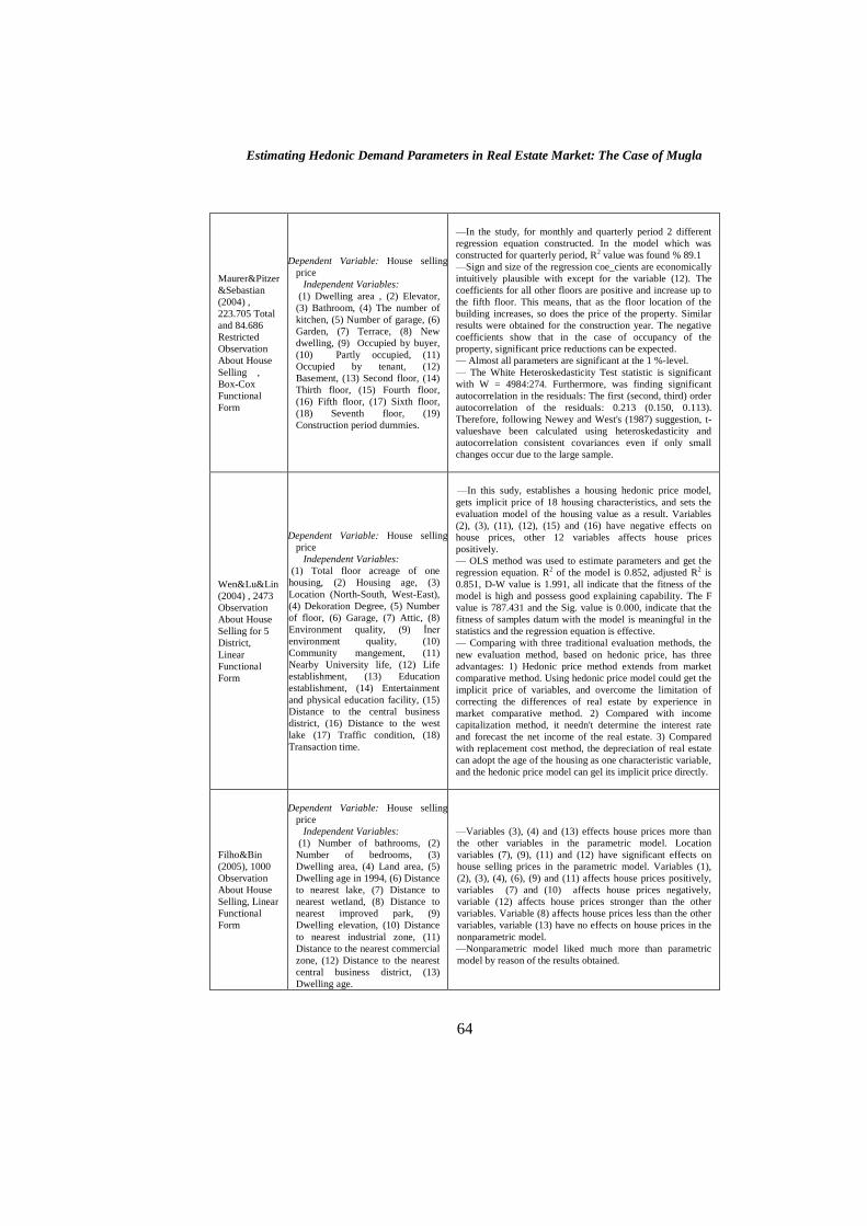
Estimating Hedonic Demand Parameters in Real Estate Market: The Case of Mugla
64
Maurer&Pitzer
&Sebastian
(2004) ,
223.705 Total
and 84.686
Restricted
Observation
About House
Selling ,
Box-Cox
Functional
Form
Dependent Variable: House selling
price
Independent Variables:
(1) Dwelling area , (2) Elevator,
(3) Bathroom, (4) The number of
kitchen, (5) Number of garage, (6)
Garden, (7) Terrace, (8) New
dwelling, (9) Occupied by buyer,
(10) Partly occupied, (11)
Occupied by tenant, (12)
Basement, (13) Second floor, (14)
Thirth floor, (15) Fourth floor,
(16) Fifth floor, (17) Sixth floor,
(18) Seventh floor, (19)
Construction period dummies.
—In the study, for monthly and quarterly period 2 different
regression equation constructed. In the model which was
constructed for quarterly period, R2 value was found % 89.1
—Sign and size of the regression coe_cients are economically
intuitively plausible with except for the variable (12). The
coefficients for all other floors are positive and increase up to
the fifth floor. This means, that as the floor location of the
building increases, so does the price of the property. Similar
results were obtained for the construction year. The negative
coefficients show that in the case of occupancy of the
property, significant price reductions can be expected.
— Almost all parameters are significant at the 1 %-level.
— The White Heteroskedasticity Test statistic is significant
with W = 4984:274. Furthermore, was finding significant
autocorrelation in the residuals: The first (second, third) order
autocorrelation of the residuals: 0.213 (0.150, 0.113).
Therefore, following Newey and West's (1987) suggestion, t-
valueshave been calculated using heteroskedasticity and
autocorrelation consistent covariances even if only small
changes occur due to the large sample.
Wen&Lu&Lin
(2004) , 2473
Observation
About House
Selling for 5
District,
Linear
Functional
Form
Dependent Variable: House selling
price
Independent Variables:
(1) Total floor acreage of one
housing, (2) Housing age, (3)
Location (North-South, West-East),
(4) Dekoration Degree, (5) Number
of floor, (6) Garage, (7) Attic, (8)
Environment quality, (9) İner
environment quality, (10)
Community mangement, (11)
Nearby University life, (12) Life
establishment, (13) Education
establishment, (14) Entertainment
and physical education facility, (15)
Distance to the central business
district, (16) Distance to the west
lake (17) Traffic condition, (18)
Transaction time.
—In this sudy, establishes a housing hedonic price model,
gets implicit price of 18 housing characteristics, and sets the
evaluation model of the housing value as a result. Variables
(2), (3), (11), (12), (15) and (16) have negative effects on
house prices, other 12 variables affects house prices
positively.
— OLS method was used to estimate parameters and get the
regression equation. R2 of the model is 0.852, adjusted R2 is
0.851, D-W value is 1.991, all indicate that the fitness of the
model is high and possess good explaining capability. The F
value is 787.431 and the Sig. value is 0.000, indicate that the
fitness of samples datum with the model is meaningful in the
statistics and the regression equation is effective.
— Comparing with three traditional evaluation methods, the
new evaluation method, based on hedonic price, has three
advantages: 1) Hedonic price method extends from market
comparative method. Using hedonic price model could get the
implicit price of variables, and overcome the limitation of
correcting the differences of real estate by experience in
market comparative method. 2) Compared with income
capitalization method, it needn't determine the interest rate
and forecast the net income of the real estate. 3) Compared
with replacement cost method, the depreciation of real estate
can adopt the age of the housing as one characteristic variable,
and the hedonic price model can gel its implicit price directly.
Filho&Bin
(2005), 1000
Observation
About House
Selling, Linear
Functional
Form
Dependent Variable: House selling
price
Independent Variables:
(1) Number of bathrooms, (2)
Number of bedrooms, (3)
Dwelling area, (4) Land area, (5)
Dwelling age in 1994, (6) Distance
to nearest lake, (7) Distance to
nearest wetland, (8) Distance to
nearest improved park, (9)
Dwelling elevation, (10) Distance
to nearest industrial zone, (11)
Distance to the nearest commercial
zone, (12) Distance to the nearest
central business district, (13)
Dwelling age.
—Variables (3), (4) and (13) effects house prices more than
the other variables in the parametric model. Location
variables (7), (9), (11) and (12) have significant effects on
house selling prices in the parametric model. Variables (1),
(2), (3), (4), (6), (9) and (11) affects house prices positively,
variables (7) and (10) affects house prices negatively,
variable (12) affects house prices stronger than the other
variables. Variable (8) affects house prices less than the other
variables, variable (13) have no effects on house prices in the
nonparametric model.
—Nonparametric model liked much more than parametric
model by reason of the results obtained.

Ercan BALDEMİR-Cüneyt Yenal KESBİÇ-Mustafa İNCİ
65
Cohen
&
Coughlin
(2005) , 2370
Total and 1643
Restricted
Observation
About House
Selling Near
The Airport,
Logarithmic,
Semi-
Logarithmic
and Linear
Functional
Forms
Dependent Variable: House sale
price deflated by median housing
price index for Atlanta
Independent Variables:
(1)The number of houses within
the 65 decibel day-night sound
level, (2) The number of houses
within the 70 decibel day-night
sound level, (3) 3 bedrooms, (4) 4
bedrooms, (5) 4 and more
bedrooms (6) 2 batrooms, (7) 3
bathrooms, (8) 3 and more
bathrooms (9) 2 and more
fireplaces, (10) Houses with more
than one story, (11) Age of house,
(12) Lot size in acres, (13)
Distance in miles from house to
airport, (14) A house was sold
occupied by blacks, (15) City
dummies, (16) Houses within the
65 decibel day-night sound level
noise contour for both 1995 and
2003, (17) Houses within the 70
decibel day-night sound level
noise contour for both 1995 and
2003, (18) Houses sold during
2000–2002 , (19) Houses sold
during 2000–2002 within the 65
decibel noise contour, (20)
Houses sold during 2000–2002
within the 65 decibel noise.
—This study using hedonic models for analyze the effects of
noise and proximity on housing prices in neighborhoods near
International Airport during 1995–2002. And addressing
complications caused by changes over time in the levels and
geographic distribution of noise and by the fact that noise
levels are measured only at the beginning and after the end of
the sample period.
—Hedonic regressions constructed for 1995–1999 and 2000–
2002 period in the study.
—Point estimates of the noise discount are sensitive to both
the functional form and the noise contours used to classify
houses in the study. proximity to the airport is related
positively to housing prices. Moreover, when this variable is
excluded, the estimated impact of noise on housing prices is
much less in absolute value than when this variable is
included.
—Generally speaking, housing prices were affected positively
by declining noise levels. After accounting for proximity,
house characteristics, and demographic variables, houses in
noisier areas sold for less than houses subjected to less noise.
—Proximity to the airport is related positively to housing
prices.
Li&Prud‘Hom
me&
Yu
(2006), 33.595
Observation
About Resale
House, Linear,
Semi-
Logarithmic,
Log-Linear and
Box-Cox
Functional
Forms
Dependent Variable: House selling
price
Independent Variables:
(1) Total square footage of living
area in the unit, (2) Total square
footage of lot area, (3) Number of
bedrooms, (4) Number of
bathrooms, (5) Number of
Garages, (6) Number of fireplaces,
(7) Number of total appliances, (8)
Age of a unit, (9) Age of a unit2
(10) Exterior finish is brick, (11)
New house, (12) Unit has
hardwood, (13) Heating fuel is
naturel gas, (14) Unit is at corner,
(15) Unit is at cul-de-sac, (16)
Terrace, (17) Distance to the
shopping center, (18)
Central/Built-in vacuum (19)
İndoor or outdoor pool, (20)
Whirlbath, (21) Sauna, (22) Air
condition system, (23) Unit is
located at downtown, (24) South,
(25) East, (26) WestDoğu, (27)
West then farwest, (28) Unit is
located at iner suburb.
— The Chow test results indicate that structural changes
between adjacent years are mild though statistically
significant.
—The pooled regression for the semi-log model, however,
results in a price index that closed matched those from
separate regressions on the annual base.
—In fact the hedonic price indexes are insensitive to structural
changes over the years and to the differences in the Laspeyres
and Paasche types formulation.
—The Box-Cox analysis rejects the linear, semilog, and log-
linear functional forms. It also suggests that the problem of
heteroskedasticity can be mitigated by choosing the more
correct functional form.
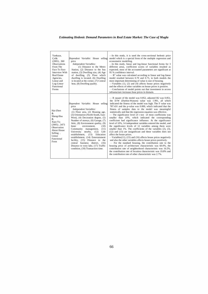
Estimating Hedonic Demand Parameters in Real Estate Market: The Case of Mugla
66
Yankaya,
Çelik
(2005) , 360
Observations
From The
Face To Face
Interview With
Real Estate
Agencies,
Linear and
Log-Linear
Functional
Forms
Dependent Variable: House selling
price
Independent Variables:
(1) Distance to the Metro
Station, (2) Distance to the bus
station, (3) Dwelling size, (4) Age
of dwelling, (5) Floor which
dwelling is located, (6) Dwelling
is located at the corner, (7) Central
heat, (8) Dwelling quality.
—In this study, it is used the cross-sectional hedonic price
model which is a special form of the multiple regression and
econometric modelling.
—In this study, linear and log-linear functional forms for 3
different areas, coefficient scores of variables resulted as
expected; most of the accounted parameters are significant at
95 % confidence interval.
— R2 value was calculated according to linear and log-linear
model resulted between 0.70 and 0.75, in both models the
most important determining of value is size of housing.
—Variables (1), (2) and (4) affects house prices negatively
and the effects of other variables on house prices is positive.
—Conclusions of model points out that investment in access
infrastucture increases hose prices in domain.
Hai-Zhen
&
Sheng-Hua
&
Xiao-Yu
(2005) , 2473
Observation
About House
Selling ,
Linear
Functional
Form
Dependent Variable: House selling
price
Independent Variables:
(1) Floor area, (2) Housing age,
(3) Orientation (North-South, East-
West), (4) Decoration degree, (5)
Number of storeys, (6) Garage, (7)
Attic, (8) Environment quality, (9)
Inner environment, (10)
Community management, (11)
University nearby, (12) Life
establishment, (13) Education
establishment, (14) Entertainment
facility, (15) Distance to the
central business district, (16)
Distance to west lake, (17) Traffic
condition, (18) Transaction time.
— R square of the model was 0.852, adjusted R2 was 0.851,
the D-W (Durbin-Watson) value was 1.991, all which
indicated the fitness of the model was high. The F value was
787.431 and the p-value was 0.000, which indicated that the
fitness of samples data to the model was meaningful
statistically and that the regression equation was effective.
— The significance level of t test of most coefficients was
smaller than 10%, which indicated the corresponding
coefficient had significance influence. At the significance
level of 10%, 14 independent variables entered the model, and
the significance levels of 12 variables among them were
smaller than 1%. The coefficients of the variables (2), (3),
(12) and (13) are insignificant and these variables does not
affect the house prices.
—Variables(11), (15) and (16) affects house prices negatively
and also the other variables affects house prices positively.
— For the standard housing, the contribution rate to the
housing price of architecture characteristic was 60.0%, the
contribution rate of neighborhood characteristic was 16.5%,
the contribution rate of location characteristic was 19.8% and
the contribution rate of other characteristic was 2.7%.