Estimating false discovery rates for contingency tables

Jonathan M. Carlson, David Heckerman and Guy ShaniMicrosoft ResearchMSR-TR-2009-53

{carlson,heckerma,guyshani}@microsoft.com

May 6, 2009

Abstract

When testing a large number of hypotheses, it can be helpful to estimate or control the false discoveryrate (FDR), the expected proportion of tests called significant that are truly null. The FDR is intricatelylinked to probability that a truly null test is significant, and thus a number of methods have been describedthat estimate or control the FDR by directly using the p-values of the hypothesis tests. Most of thesemethods make the assumption that the p-values are uniformly and continuously distributed under the nullhypothesis, an assumption that often does not hold for finite data. In this paper, we consider the estimationof FDR for contingency tables. We show how Fisher’s exact test can be extended to efficiently calculatethe exact null distribution over a set of contingency tables. Using this exact null distribution, we explorethe estimation of each of the terms in the FDR estimation, characterize the asymptotic convergence of theestimator, and show how the conservative bias can be reduced by removing certain tests from consideration.The resulting estimator has substantially less conservative bias than traditional approaches.

1 IntroductionIn modern biomedical applications, researchers often want to test multiple hypotheses at the same time. Forexample, in an HIV drug resistance study, a researcher may wish to test which observed HIV mutations arecorrelated with drug resistance. The p-value, the probability of getting a result at least as extreme as theobserved test assuming the null hypothesis is correct, can be used to filter out low probability correlations.Researchers typically consider the subset of tests with p-value below some threshold for a follow-up study.When performing multiple statistical tests, these p-value thresholds must be carefully chosen so as to avoidan abundance of false positive results, while at the same time maximizing the number of true positive results.Traditionally, p-value thresholds are chosen so as to control the probability of at least one false positive result.More recently, Benjamini & Hochberg (1995) proposed controlling the false discovery rate (FDR), which isthe expected proportion of false positives among tests that are called significant. Storey (2002, 2003) intro-duced the FDR-analogue of the p-value, called the q-value, which estimates the minimum FDR for any givenp-value threshold. This approach has proven widely applicable in, for example, high throughput biologicalscreens, as it allows a researcher to balance the number of significant associations with the proportion ofthose tests that are expected to be false positives.

When test statistics are continuous and two-sided, the p-values are expected to be uniformly distributedunder the null hypothesis. For these cases, Storey (2002, 2003) provides a simple procedure for estimating theFDR. For many emerging biological applications, however, the underlying test statistics are not continuous.For example, tests involving genetic data (such as single nucleotide polymorphisms, or SNPs) often involve asmall number of possible outcomes. As we will later illustrate, in such cases the discreteness in the data willcause the p-values under the null hypothesis to be heavily skewed toward one, making Storey’s FDR methodoverly conservative (Pounds & Cheng, 2006; Gilbert, 2005). Furthermore, it is often the case that each testwill have a different p-value distribution under the null hypothesis, further complicating analysis.

1

Although the discreteness of the data presents unique challenges, we can also leverage it to our advantage.For many discrete tests the exact null distribution can be efficiently computed. We can use these exactcomputations to provide tighter FDR estimates. In this paper, we consider those cases where the sufficientstatistics for a test are a 2×2 contingency table and Fisher’s exact test (FET) is appropriate. In these cases, weshow how FET can be leveraged to efficiently compute an FDR estimator that is asymptotically conservativeand yields more power than estimations that are based on continuous assumptions.

FET uses the hypergeometric distribution to estimate the null distribution of a single test using all thepossible permutations of that test’s data. We extend this null distribution to efficiently compute the exactType I error rate over a large number of tests. We demonstrate it’s applicability to discrete data, provide anefficient implementation for exact permutation testing, and prove the asymptotically conservative result. Wesuggest a family of permutation-based estimators for the π0 parameter, estimating the proportion of all teststhat are truly null. We explore the convergence properties of our estimators and discuss their convergenceproperties.

One of the unique advantages of discrete data is the potential to ignore tests than can be proven to be irrel-evant. We derive a new filtering criterion that is provably conservative and will, under certain circumstances,provably increase power.

Although this paper focuses on Fisher’s exact test over binary contingency tables, our theoretical resultswill generalize to other exact tests, such as McNamara’s test and the exact test for Hardy-Weinberg Equilib-rium, for which exact distributions can be efficiently calculated.

2 Multiple Hypothesis ExamplesTo demonstrate the applicability of our methods, we experiment with the following data sets:

HIV resistance. A number of effective antiretroviral (ARV) drugs have been developed for HIV. How-ever, for each of these drugs there exists a set of HIV mutations that abrogate the drug’s effectiveness. Thus,an active area of research involves the identification and characterization of drug resistance mutations. Har-rigan and colleagues (Harrigan et al., 2005) enrolled patients at the start of their ARV therapy and sequencedthe infecting HIV genomes. After several years of therapy on multiple classes of ARVs, the researchers re-sequenced the infecting HIV genomes to identify mutations that were correlated with specific ARVs. Theytested whether the presence of a mutation at a given position in the HIV genome was correlated with thepatient taking a specific ARV. Three classes of drugs were tested over 1194 variables representing observedamino acids at positions in the HIV Protease and Reverse Transcriptase proteins, resulting in 3582 total tests,each with 281 observations. We will refer to this data set as “Resistance”.

Epitope mapping. The cellular arm of the immune response identifies and destroys infected cells. Suchcells can be identified by the unique strings of viral protein fragments, called epitopes, that are displayedon the surface of infected cells. These epitopes are displayed by human leukocyte antigen (HLA) proteins.Thousands of HLA variations have been identified in humans. Thus, a critical component of HIV vaccinedesign is the identification and characterization of the set of epitopes that each HLA allele can present on thecell surface.

One high-throughput experimental method for epitope mapping is the use of overlapping peptide (OLP)scans, in which a sliding window of 10-15 amino acid peptide fragments are created based on the viralgenome of interest. Each OLP is then tested against cells from dozens of patients, each of whom contains sixHLA alleles, with an assay that tests if at least one of the HLA proteins binds the peptide (Addo et al., 2003).One then attempts to map HLA alleles to positive assay responses. The test can be performed using FET,comparing the frequency of response to an epitope in patients with or without a given HLA allele. Kiepielaet al. (2007) recently performed this high throughput assay. Here, we reanalyze their data, comparing com-paring 219 HLA alleles with 343 OLPs, resulting in 74,774 total tests, with an average of 724 observationsper test. This data set is denoted “Epitope”.

Sieve analysis. In sieve analysis we try to identify positions in the viral genome at which the variabilitydiffers between two different populations (Gilbert, 2005). For example, if the position is more variable in

2

patients from one region than those from another, it may indicate that different forces are acting on thatregion. Following Gilbert, we have created a data set consisting of 567 HIV clade B sequences (Brummeet al., 2008) and 567 HIV clade C sequences (Kiepiela et al., 2007; Rousseau et al., 2008) and, for 363positions in the HIV Gag protein, compared the frequency at which sequences match the consensus for theirrespective clades. We will call this data set “Sieve”.

Linkage disequilibrium mapping. Linkage disequilibrium (LD) occurs when two sites on a chromo-some are not statistically independent of each other. This typically occurs when the sites are nearby on thechromosome, such that inheritance of a given allele at one site is correlated with inheritance of a given alleleat the other site. When performing genome wide association studies (GWAS), it is helpful to identify a set ofvariations (SNPs) that are in LD with each other, so that potentially redundant results can be identified. Wehave taken the SNP data from a recent GWAS (Chio et al., 2009), binarized the data and tested for indepen-dence between each of 401,017 pairs of neighboring SNPs. There was an average of 1085 observations pertest. We will call this data set “SNP”.

Synthetic data We also created various types of synthetic data based on the Epitope data set (see Ap-pendix). Through such synthetic data we can demonstrate each aspect of our proposed approach.

3 Background

3.1 Contingency Tables and Fisher’s Exact TestConsider an experiment that tests the independence of two random binary variables X and Y . Suppose thereare n observations, (x1, y1), (x2, y2), . . . , (xn, yn). The results can be summarized in a contingency tablet = (a, b, c, d), as defined in Table 1. We denote the marginal counts of t as θt = (θX , θX , θY , θY ), whichrepresent the number of times each variable is observed in each state. These counts capture the maximumlikelihood estimators for the marginal probabilities pr(X = 1) and pr(Y = 1). We will often drop the super-script t when it is clear from context.

Table 1: 2× 2 contingency table

Y = 1 Y = 0∑X

X = 1 a b θX = a+ b

X = 0 c d θX = c+ d∑Y θY = a+ c θY = b+ d n

Our goal is to test the null hypothesisH = 0 thatX and Y are independent. Let T be the random variablerepresenting a table with marginals θ. Fisher (1922) showed that, if X and Y are independent and each isindependent and identically distributed (IID), then the probability pr(t) of observing T = t is given by thehypergeometric distribution:

pr(t) ,

(θt

Xa

)(θt

Xc

)(nθt

Y

) . (1)

From (1), a two-tailed marginal p-value p(t) can be computed for t using

p(t) ,∑

t′∈perm(t)

pr(t′)1{pr(t′) ≤ pr(t)} , (2)

where perm(t) = {t′ : θt′

= θt}, and 1{·} is the indicator function that evaluates to one if the constraints aresatisfied and 0 otherwise. We call Equation (2) a marginal p-value because it is conditioned on the marginalsθ.

3

Many statistics have a uniform distribution of p-values under the null. That is, if P is a continuous randomvariable representing a p-value, pr(P ≤ α | H = 0) = α. It is evident from (1), however, that the distributionof FET p-values under the null may be strongly skewed toward one and therefore pr(P ≤ α | H = 0) ≤ α.For example, the minimum achievable p-value for a given n is 1/

(nn/2

), and that can only be achieved when

the marginals are evenly distributed (i.e., when θX = θX = n2 ). Figure 1 shows the distribution of p-values

from our various data sets.

0

100

200

300

400

500

0-1-2-3-4-5-6-7-8-9

(a) Resistance

0

500

1000

1500

2000

0-1-2-3-4-5-6-7-8-9

(b) Epitope

0

25

50

75

100

0-1-2-3-4-5-6-7-8-9

(c) Sieve

0

5000

10000

15000

20000

0-1-2-3-4-5-6-7-8-9

(d) SNPs

Figure 1: The histogram of marginal p-values for the various data sets. p-values are transformed using log2 p.

3.2 Positive False Discovery RatesSuppose that m hypothesis tests over 2 × 2 contingency tables t1, . . . , tm are simultaneously tested usingFisher’s exact test, with corresponding marginal p-values p1, p2, . . . , pm, and we wish to estimate or controlthe false positive rate in some way. Given the values of H = 1, H2, . . . ,Hm, where Hi = 0 if the ith nullhypothesis is true and Hi = 1 if the null hypothesis is false, and a rejection region Γ, the possible results aresummarized in Table 2.

Note that only m, R and W are observed. Here, we will focus on nested rejection regions defined by theType I error rate α. That is, given an α ∈ [0, 1], we will reject all tests with P ≤ α. For convenience, we will

4

Table 2: Outcomes when testing m hypotheses

Hypothesis Accept Reject TotalNull true U(Γ) V (Γ) m0

Alternative true T (Γ) S(Γ) m1

Total W (Γ) R(Γ) m

use α to denote this rejection region.Benjamini & Hochberg (1995) proposed controlling the False Discovery Rate (FDR), which they defined

to be

FDR(α) , E

(V (α)R(α)

).

When R(α) = 0, this quantity is undefined. In this case, Benjamini and Hochberg defined FDR(α) to be 0,which is equivalent to defining

FDR(α) , E

(V (α)R(α)

∣∣∣∣ R(α) > 0)

pr(R(α) > 0) .

In practice, we are only interested in p-value thresholds that result in the rejection of at least one test in ourdata. Thus, Storey (2002) proposed the positive false discovery rate (PFDR), which is conditioned on therejection of at least one test:

PFDR(α) = E

(V (α)R(α)

∣∣∣∣ R(α) > 0)

=1

pr(R(α) > 0)FDR(α).

Following Storey (2002), assume that the random variables Hi are IID Bernoulli variables with priorprobability pr(Hi = 1) = 1− π0 and that the p-values are IID with

Pi | Hi ∼ (1−Hi)F0 +HiF1,

for some null distribution F0 and some alternative distribution F1. Under these assumptions, Storey (2002)showed that

PFDR(α) = pr(H = 0 | P ≤ α)

=π0 pr(P ≤ α | H = 0)

pr(P ≤ α)(3)

= E(V (α))E(R(α))

.

For small samples, it may be quite likely that no tests are rejected at threshold α. Therefore, Storey (2002)proposed the following estimator for PFDR:

PFDR(α) ,π0 pr(P ≤ α | H = 0)

pr(P ≤ α) pr(R(α) > 0). (4)

Equation (4) provides estimators for each term of (3), with an added correction term that estimates pr(R(α) > 0).(Note that for large m, PFDR ≈ FDR, because pr(R(α) > 0) ≈ 1.)

For p-values that are not biased towards 0 under the null distribution, Storey (2002) showed that

PFDR(α) ,W (λ) α

(1− λ)R(α) (1− (1− α)m),

5

for some well-chosen λ, 0 ≤ λ < 1, is conservative both asymptotically and in expectation for finite samplesusing the intuition that pr(P ≤ α | H = 0) ≤ α and π0 ≈ W (λ)

(1−λ)m . Storey (2002); Storey & Tibshirani(2003) and others (e.g., Langaas et al. 2005) have proposed methods for choosing λ.

In practice, Storey suggested estimating PFDR(α) for each observed p-value pi and proved that, under theaforementioned independence assumptions, the estimates are simultaneously conservative for all pi Storeyet al. (2004). When the tests are continuous and uniformly distributed, pr(P ≤ pi | H = 0) = pi, makingStorey’s estimator quite tight in practice. When the tests are discrete, however, pr(P ≤ pi | H = 0) canbe significantly less than α. For example, in the case of Fisher’s exact test, each observed p-value pi is amarginal p-value dependent on the marginals θi. Although pr(P ≤ pi | H = 0, θi) = pi, for some test j 6= i,pr(P ≤ pi | H = 0, θj) ≤ pi. Thus, the overall probability pr(P ≤ Pi | H = 0) ≤ pi, making Storey’sestimate overly conservative.

4 Computing PFDR for Fisher’s exact testFisher’s exact test provides an efficient means of computing pr(P ≤ α | H = 0, θ) exactly. Although theresulting marginal p-values should not be applied directly to PFDR estimation, the computation can be ef-ficiently leveraged to provide a tight estimate for each of the terms in (4). In this section, we define eachof these estimates and show that each estimate is unbiased or conservative (in this context, an estimator isconservative if it is expected to overestimate terms in the numerator of (4) or underestimate terms in thedenominator of (4)). We evaluate the asymptotic convergence properties of (4), showing that it results in aconservative FDR estimate and characterize conditions under which the estimates will be closer to the truevalues. In addition, we discuss ways in which the exact test can be further leveraged to increase power byfiltering irrelevant tests.

Assumption 1. We assume that p-values are IID and the Hi are IID Bernoulli random variables. Because weare using Fisher’s exact test, we also need to consider the marginals θ, which we assume are IID. Althoughwe we make no assumptions about the specific distribution of θ, we assume that the p-values depend on themarginals according to the mixture model

P | H, θ ∼ (1−H)F0(θ) +HF1(θ) (5)

where F0(θ) follows the hypergeometric distribution as defined in (2) and F1(θ) is the generating functionof the alternative model. We further assume that θ is independent of H, though we will later relax thisassumption.

4.1 Estimating pr(P ≤ α | H = 0) from pooled p-valuesThe typical approach to FDR estimation is to assume for each pi that pr(P ≤ pi | H = 0) = pi, which isequivalent to assuming pr(P ≤ α | H = 0) = pr(P ≤ α | H = 0, θj) for j = 1, . . . ,m. It is evident fromequation (2), however, that the p-values are not independent of the marginals. Thus, more accurate estimateis to sum out the marginals:

pr(P ≤ α | H = 0) =∑θ′

pr(P ≤ α | H = 0, θ′) pr(θ′ | H = 0) (6a)

=∑θ′

pr(P ≤ α | H = 0, θ′) pr(θ′) , (6b)

where (6b) follows from the assumption that the marginals are independent and identically distributed. Fur-thermore, this IID assumption allows us to construct an unbiased estimate using pooled p-valued, calculated

6

from

pr(P ≤ α | H = 0) =∑θ′

pr(P ≤ α | H = 0, θ′) pr(θ′) (7a)

=∑θ′

pr(P ≤ α | H = 0, θ′)

(1m

m∑i=1

1{θi = θ′}

)(7b)

=1m

m∑i=1

∑θ′

pr(P ≤ α | H = 0, θ′)1{θi = θ′} (7c)

=1m

m∑i=1

pr(P ≤ α | H = 0, θi) (7d)

where we estimate pr(θ) using the maximum likelihood estimate

pr(θ) ,1m

m∑j=1

1{θj = θ} .

Because pr(θ) is an unbiased estimator for pr(θ), it follows that

E(pr(P ≤ α | H = 0)) = pr(P ≤ α | H = 0) . (8)

Equation (7d) can be written

pr(P ≤ α | H = 0) =1m

m∑i=1

∑t′∈perm(ti)

pr(pr(t′) | H = 0)1{p(t′) ≤ α} ,

indicating that the pooled p-value is taken from every possible permutation of the data. Note that the right-most summation is itself a p-value and the constraint 1{p(T ′) ≤ α} is such that the summation is the maxi-mum achievable p-value under θi that is at most α. Thus,

E(pr(P ≤ α | H = 0)) ≤ α (9)

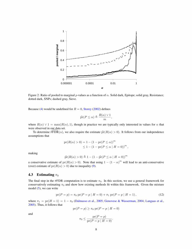
with equality when all the observed marginals can achieve α exactly. Thus, when not all marginals canachieve α exactly, power can be gained over the marginal p-values by using the pooled p-values, which yielda tighter estimate of pr(P ≤ α | H = 0). The specific reduction in bias can be expressed as the ratio

pr(P ≤ α | H = 0)α

, (10)

which can have quite a large effect in practice, especially for small α. Figure 2 plots this ratio as a functionof α for each of our data sets.

4.2 Estimating pr(P ≤ α) and pr(R(α) > 0)

Given that R(α) is the number of observed tests with p ≤ α, it follows that

E

(R(α)m

)= pr(P ≤ α) . (11)

We therefore follow Storey (2002) in defining

pr(P ≤ α) ,R(α)m

.

7

0

0.2

0.4

0.6

0.8

1

0.000001 0.0001 0.01 1

po

ole

d / m

arg

inal

𝜶

Figure 2: Ratio of pooled to marginal p-values as a function of α. Solid dark, Epitope; solid gray, Resistance;dotted dark, SNPs; dashed gray, Sieve.

Because (4) would be undefined for R = 0, Storey (2002) defines

pr(P ≤ α) ,R(α) ∨ 1

m,

where R(α) ∨ 1 = max(R(α), 1), though in practice we are typically only interested in values for α thatwere observed in our data set.

To determine PFDR(α), we also require the estimate pr(R(α) > 0). It follows from our independenceassumptions that

pr(R(α) > 0) = 1− (1− pr(P ≤ α))m

≤ 1− (1− pr(P ≤ α | H = 0))m ,

makingpr(R(α) > 0) , 1− (1− pr(P ≤ α | H = 0))m

a conservative estimate of pr(R(α) > 0). Note that using 1 − (1− α)m will lead to an anti-conservative(over) estimate of pr(R(α) > 0) due to inequality (9).

4.3 Estimating π0

The final step in the PFDR computation is to estimate π0. In this section, we use a general framework forconservatively estimating π0 and show how existing methods fit within this framework. Given the mixturemodel (5), we can write

pr(P = p) = π0 pr(P = p | H = 0) + π1 pr(P = p | H = 1) , (12)

where π1 = pr(H = 1) = 1 − π0 (Dalmasso et al., 2005; Genovese & Wasserman, 2004; Langaas et al.,2005). Thus, it follows that

pr(P = p) ≥ π0 pr(P = p | H = 0)

and

π0 ≤pr(P = p)

pr(P = p | H = 0).

8

Moreover, for any non-negative function ρ(·),

π0 ≤∑p ρ(p)pr(P = p)∑

p ρ(p)pr(P = p | H = 0), (13)

which leads to the following lemma.

Lemma 1. Suppose we have m tests that follow Assumption 1. Let ρ(·) be any non-negative function, and

π0 ,

∑mi=1 ρ(pi)∑m

i=1E(ρ(p) | H = 0, θi). (14)

Then E(π0) ≥ π0.

Proof. It follows analogously to the derivation of (7) that

pr(P = p | H = 0) =1mE

(m∑i=1

pr(P = p | H = 0, θi)

)(15)

and

pr(P = p) =1mE

(m∑i=1

1{pi = p}

). (16)

Thus, combining with inequality (13), it follows that

π0 ≤∑p ρ(p)pr(P = p)∑

p ρ(p)pr(P = p | H = 0)=

∑p ρ(p) 1

m E(∑mi=1 1{pi = p})∑

p ρ(p) 1m E(

∑mi=1 pr(P = p | H = 0, θi))

(17a)

= E(∑mi=1 ρ(pi))

E(∑m

i=1

∑p ρ(p)pr(P = p | H = 0, θi)

) . (17b)

Because∑p ρ(p)pr(P = p) is a linearly increasing function of

∑p ρ(p)pr(P = p | H = 0), it follows from

Jensen’s inequality that

E(∑mi=1 ρ(pi))

E(∑m

i=1

∑p ρ(p)pr(P = p | H = 0, θi)

) ≤ E( ∑mi=1 ρ(pi)∑m

i=1

∑p ρ(p)pr(P = p | H = 0, θi)

)

=∑mi=1 ρ(pi)∑m

i=1E(ρ(p) | H = 0, θi)

= π0.

Thus, E(π0) ≥ π0.

Furthermore, in the limit, estimate (14) asymptotically converges to

π0 + π1E(ρ(p) | H = 1)E(ρ(p) | H = 0)

,

which implies that the ρ(·) function minimizing E(ρ(p) | H=1)

E(ρ(p) | H=0) will yield the least biased estimator.

Lemma 2. Under the assumptions of Lemma 1,

limm→∞

π0a.s.= π0 + π1

E(ρ(p) | H = 1)E(ρ(p) | H = 0)

.

9

Proof. By the strong law of large numbers, equations (15) and (16) imply thatm−1E(∑mi=1 pr(P = p | H = 0, θi))

and m−1E(∑mi=1 1{pi = p}) converge almost surely to pr(P = p | H = 0) and pr(P = p), respectively.

Thus, it follows from (17) that

limm→∞

π0a.s.=

∑p ρ(p)pr(P = p)∑

p ρ(p)pr(P = p | H = 0).

Furthermore, it follows from the mixture model (12) that∑p ρ(p)pr(P = p)∑

p ρ(p)pr(P = p | H = 0)= π0 + π1

∑p ρ(p)pr(P = p | H = 1)∑p ρ(p)pr(P = p | H = 0)

. (18)

Thus,

limm→∞

π0a.s.= π0 + π1

∑p ρ(p)pr(P = p | H = 1)∑p ρ(p)pr(P = p | H = 0)

= π0 + π1E(ρ(p) | H = 1)E(ρ(p) | H = 0)

.

Equation (14) gives us great flexibility in computing π0 estimates. One such estimation method is givenby Storey (2002, 2003)

π0(λ) =#{pi > λ}(1− λ)m

(19)

for some tuning parameter 0 ≤ λ < 1. For uniformly distributed statistics,

(1− λ)m = E(#{π > λ} | H = 0) = m pr(P > λ | H = 0) .

For contingency tables, we can estimate pr(P > λ | H = 0) using pr(P ≤ λ | H = 0), which results inan unbiased estimate for E(#{π > λ} | H = 0). Therefore, Storey’s estimator (19) is a special case ofestimator (14) in which

ρ(p) =

{0 if p ≤ λ,1 otherwise

and the P-values are assumed to be continuous and uniformly distributed under the null.As λ → 0, we have increasingly conservative bias, with π0 = 1 when λ = 0, whereas the variance of

the π0 estimate increases as λ→ 1 due to the decreasing number of observations. Indeed, different heuristicapproaches have been proposed to balance the bias-variance tradeoff inherent in picking λ (Storey, 2002;Storey & Tibshirani, 2003). Equation (14) suggests an orthogonal heuristic that may be useful in estimatingπ0: choosing a weighting function ρ(·) such that more weight is applied to tests with high p-value. A naturalchoice for a weighting function is ρ(p) = pr(P ≤ p | H = 0, θi) = pi, which is equivalent to

π0 ,E(p)

E(p | H = 0). (20)

Under this weighting function, tests with low p-values will still contribute to the π0 estimate, but not as muchas tests with high p-values. In principle, we could define ρ(·) such that we are effectively summing p-valuesover the range λ < p ≤ 1; in practice, however, we have found the π0 estimate to be quite stable over a widerange of λ, and so simply set λ = 0.

Pounds & Cheng (2006) suggested the estimator π0 , 2p for discrete statistics, where p is the averageobserved marginal p-value. Estimator (20) is similar to their estimate, except that for contingency tables wecan compute E(p | H = 0) exactly, rather than assuming E(p | H = 0) = 0.5, which assumes a unformdistribution of p-values.

10

Table 3 compares the true π0 for synthetic data against the π0 estimators of equation (14), of Storey(2003) (evaluated for λ = 0.51) and of Pounds & Cheng (2006) computed using marginal p-values. Equation(14) provides a tight and conservative estimate, substantially increasing power over methods that assume auniform p-value distribution. Similarly, accounting for the exact p-value distribution results in a substantiallylower π0 estimate on each of the real data sets (Table 3).

Table 3: Comparing π0 estimates

Data set E(P )

E(P |H=0) 2p Storeya

0.001b 0.086 0.12 0.110.05 0.13 0.18 0.170.1 0.18 0.25 0.240.2 0.27 0.38 0.370.3 0.36 0.52 0.510.4 0.45 0.64 0.630.5 0.58 0.69 0.680.6 0.66 0.79 0.790.7 0.75 0.91 0.900.8 0.83 1.01 10.9 0.92 1.13 11 1.003 1.24 1Sieve 0.63 0.82 0.69SNPs 0.34 0.44 0.41Epitope 0.99 1.84 1Resistance 0.97 1.38 1

aEvaluated at λ = 0.5 using pooled p-values.bNumeric data sets indicate π0 for synthetic

data derived from the Epitope data set.

4.4 Convergence propertiesWe have presented estimates for each component of PFDR, showing how each is either unbiased or conser-vative. It follows that PFDR is asymptotically conservative as m → ∞. We can, however, be more precisein estimating the convergence properties of our PFDR estimate.

Theorem 1. Given m tests that follow Assumption 1 and a non-negative function ρ(·), we have

limm→∞

PFDR(α) a.s.=π0 + π1

E(ρ(p) | H=1)

E(ρ(p) | H=0)

π0PFDR(α).

This convergence theorem shows that, for large samples, our PFDR estimate is conservative and becomestightest when π0 is computed using a ρ(·) function that is expected to be much lower for true alternativehypotheses than for true null hypotheses.

1We used the available R code from http://genomics.princeton.edu/storeylab/qvalue/index.html, using pooled p-values as input. Re-sults are truncated at 1. λ = 0.5 was chosen because the spline-fitting method Storey & Tibshirani (2003) always results in estimates ofπ0 = 1 for these discrete data sets.

11

Proof.

limm→∞

PFDR(α) = limm→∞

π0 pr(P ≤ α | H = 0)pr(P ≤ α) pr(R(α) > 0)

=limm→∞ π0 limm→∞ pr(P ≤ α | H = 0)

limm→∞ pr(P ≤ α) limm→∞ pr(R(α) > 0).

By the strong law of large numbers, equation (8) implies that pr(P ≤ α | H = 0) converges almost surelyto pr(P ≤ α | H = 0), equation (11) implies that pr(P ≤ α) converges almost surely to pr(P ≤ α), andpr(R(α) > 0) converges almost surely to 1. Thus

limm→∞

PFDR(α) a.s.=limm→∞ π0 pr(P ≤ α | H = 0)

pr(P ≤ α)

=limm→∞ π0

π0PFDR(α).

Finally, it follows from Lemma 2 that

limm→∞

PFDR(α) a.s.=π0 + π1

E(ρ(p) | H=1)

E(ρ(p) | H=0)

π0PFDR(α).

4.5 Dependent marginalsUntil now, we have assumed that θ is independent of H . It is conceivable, however, that true alternativetests will tend to have more balanced marginals that permit lower p-values. For example, in the Resistancedata, it is possible that positions in which no mutations confer drug resistance may be more conserved dueto purifying selection, an evolutionary process that results in less observed variation. Under these condi-tions, we might expect the PFDR estimate to become more conservative because a substantial proportion ofthe balanced marginals included in our pooled-p-value estimate belong to true alternative tests causing usto overestimate pr(P ≤ α | H = 0). This conservative bias is analogous to that observed in the microarraycommunity—a bias that arises from permutation testing over alternative data that has a higher variance thanthe null data (Jiao & Zhang, 2008; Xie et al., 2005). In this section, we formalize the problem for discretestatistics and show that our PFDR estimate becomes asymptotically more conservative as the tendency in-creases for true alternative tests to have more evenly distributed marginals than null tests. Note that theseresults hold only for π0 estimators in which ρ(·) is non-decreasing, a slightly more restrictive definition thanwe used in the previous sections. In principle, the conservative bias could be reduced using heuristic mea-sures similar to those proposed in the microarray community (Jiao & Zhang, 2008; Xie et al., 2005); however,these heuristics are not guaranteed to result in a conservative PFDR estimate, so we will not explore themfurther here.

Let us consider a special case in which pr(θ | H = 1) 6= pr(θ | H = 0). Specifically, we shall con-sider the case where the marginals of true alternative hypotheses tend to have larger n and/or are morebalanced, meaning that the marginals of the true alternative hypotheses tend to permit smaller p-values thanthe marginals of the true null hypotheses. This leads to the following set of assumptions:

Assumption 2. Assume we have m tests, in which the P-values are independent and identically distributedaccording to the mixture (5), the H are independent and identically distributed Bernoulli random variables,and for each test i, Hi is dependent on θi such that∑

θ

pr(P ≤ α | H = 0, θ) pr(θ | H = 0) ≤∑θ

pr(P ≤ α | H = 0, θ) pr(θ | H = 1) .

Under these assumptions, we can derive the following large sample theorem:

12

Theorem 2. Given m tests that follow Assumption 2, and a non-negative, non-decreasing function ρ(·),

limm→∞

PFDR(α) ≥π0 + π1

E(ρ(p) | H=1)

E(ρ(p) | H=0)

π0PFDR(α).

Proof. The proof follows analogously to that of Theorem 1 by noting that the Assumption 2 leads to

limm→∞

pr(P ≤ α) a.s.= pr(P ≤ α) (21)

limm→∞

pr(P ≤ α | H = 0)a.s.≥ pr(P ≤ α | H = 0) (22)

limm→∞

π0

a.s.≥ π0 + π1

E(ρ(p) | H = 1)E(ρ(p) | H = 0)

. (23)

We shall prove each of these statements in turn.Equation (21) follows immediately by noting that our estimate pr(P ≤ α) , (R ∨ 1)/m is not affected

by the distribution of θ. Equation (22) can be seen by noting that we can no longer use equality (6b) and mustinstead use equality (6a).

Thus, we have

limm→∞

pr(P ≤ α | H = 0)

a.s.=∑θ′

pr(P ≤ α | H = 0, θ′) pr(θ′)

=∑θ′

pr(P ≤ α | H = 0, θ′)×{

pr(θ′ | H = 0)π0 + pr(θ′ | H = 1)π1

}= π0

∑θ′

pr(P ≤ α | H = 0, θ′) pr(θ′ | H = 0) + π1

∑θ′

pr(P ≤ α | H = 0, θ′) pr(θ′ | H = 1)

≥ π0

∑θ′

pr(P ≤ α | H = 0, θ′) pr(θ′ | H = 0) + π1

∑θ′

pr(P ≤ α | H = 0, θ′) pr(θ′ | H = 0)

= pr(P ≤ α | H = 0) ,

where the inequality follows from Assumption 2. Finally, inequality (23) follows from the fact that the addedassumptions of Lemma 2 only affect the denominator of our π0 estimate (14). Furthermore, inequality (22)implies

limm→∞

pr(P ≥ α | H = 0)a.s.≤ pr(P ≥ α | H = 0) ,

from which it follows that

limm→∞

∑p

ρ(p)pr(P = α | H = 0)a.s.≤∑p

ρ(p)pr(P = α | H = 0)

for any non-decreasing function ρ(p). Thus, it follows that

limm→∞

π0 =

∑p ρ(p)pr(P ≥ α)∑

p ρ(p)pr(P ≥ α | H = 0)

a.s.≥

∑p ρ(p)pr(P ≥ α)∑

p ρ(p)pr(P ≥ α | H = 0)

= π0 + π1E(ρ(p) | H = 1)E(ρ(p) | H = 0)

.

Hence, under Assumption 2, and provided ρ(p) is non-negative and non-decreasing in p, our PFDR andFDR estimates will be asymptotically more conservative than the case where the marginals are independentof H . In practice, it is not known whether H and θ are independent. Consequently, we recommend using themore restricted class of ρ(·) functions allowed by Theorem 2.

13

0.4

0.5

0.6

0.7

0.8

0.9

1

0.0001 0.001 0.01 0.1 1

𝝅 𝟎(𝜶)

𝝅 𝟎(𝟏)

𝜶

Figure 3: The proportional reduction in the PFDR estimate from using π0(α) (filtering) over π0(1) (notfiltering) on synthetic data derived from: solid dark, Epitope; solid gray, Resistance; dotted dark, SNPs;dashed gray, Sieve.

4.6 Filtering irrelevant testsThe discreteness of the data provides a unique opportunity to further increase power. For any discrete test,there exists an α such that pr(P ≤ α) = 0. Including such tests in our PFDR estimate will typically increasethe conservative bias. Thus, power can often be improved by first filtering out all all tests that couldn’tpossibly achieve the significance threshold α. Such filtering will still result in an asymptotically conservativeestimate and, in some cases, will provably increase power.

Because the range of the data is finite, computation of the most significant achievable p-value giventhe marginals is possible. We can define the minimum achievable p-value for fixed marginals as p∗(θ) ,mint∈perm(θ) p(t). When computing PFDR(α), we can ignore (filter) all tests i such that p∗(θi) > α. For aset of contingency tables T, we can now write T = T+

α ∪T−α for the disjoint sets

T+α = {ti : ti ∈ T ∧ p∗(θi) > α},

T−α = {ti : ti ∈ T ∧ p∗(θi) ≤ α}.

Filtering on p∗(θ) > α can be seen as estimating PFDR over T−α . Let PFDR∗(α) and PFDR∗(α) be the true

and estimated PFDR, respectively, for T−α . Then the following theorem holds.

Theorem 3. Given m tests that follow Assumptions 1 or 2, PFDR∗(α) = PFDR(α).

Proof. Recall that, under either set of assumptions,

PFDR(α) = E(V (α))E(R(α))

.

Because E(R(α) | pr(p(T ) ≤ α) = 0) = 0, it follows that PFDR(α) will be the same for T and T−α .Therefore, PFDR∗(α) = PFDR(α).

Therefore, filtering on p∗(θi) > α) does not change the true PFDR. Furthermore, under the assumptionsof Lemma 4, we have PFDR∗(α) ≤ limm→∞ PFDR

∗(α), almost surely. Consequently, we can compute

PFDR∗(α) instead of PFDR(α). Moreover, in certain cases filtering will provably increase power.

14

Lemma 3. Under assumptions 1 or 2, if pr(P≤α|H=1)pr(P≤α|H=0) is non-increasing in α, then limm→∞ PFDR

∗(α)

a.s.≤

limm→∞ PFDR(α).

Proof. Recall our large sample estimate

PFDR(α) =π0 pr(P ≤ α | H = 0)

pr(P ≤ α)

=π0 m

1m

∑mi=1 pr(P ≤ α | H = 0, θi)R(α) ∨ 1

=π0

∑mi=1 pr(P ≤ α | H = 0, θi)

R(α) ∨ 1

Removing k tests with p∗(θ) > α will have no effect on (R(α) ∨ 1) or on

m∑i=1

pr(P ≤ α | H = 0, θi) .

We will show, however, that, under the present assumptions, our π0 estimate under filtering will almost surelybe lower than our π0 estimate without filtering. Let p+ denote the event p∗(θ) > α and p− denote the eventp∗(θ) ≤ α. From equation (18)

limm→∞

π0a.s.= π0 + π1

E(ρ(p) | H = 1)E(ρ(p) | H = 0)

(24a)

= π0 + π1E(ρ(p) | H = 1, p+) pr(p+) + E(ρ(p) | H = 1, p−) pr(p−)E(ρ(p) | H = 0, p+) pr(p+) + E(ρ(p) | H = 0, p−) pr(p−)

(24b)

Let

π0(α) ,E(ρ(p) | p−)

E(ρ(p) | H = 0, p−)

be the estimated π0 over T−α . We wish to show that

limm→∞

π0(α) ≤ limm→∞

π0(1), (25)

which, by (24b) is true if an only if

E(ρ(p) | H = 1, p+) pr(p+) + E(ρ(p) | H = 1, p−) pr(p−)E(ρ(p) | H = 0, p+) pr(p+) + E(ρ(p) | H = 0, p−) pr(p−)

≥ E(ρ(p) | H = 1, p−)E(ρ(p) | H = 0, p−)

.

Thus, it follows that (25) is true if and only if

E(ρ(p) | H = 1, p+)E(ρ(p) | H = 0, p+)

≥ E(ρ(p) | H = 1, p−)E(ρ(p) | H = 0, p−)

. (26)

The assumption that pr(P≤α|H=1)pr(P≤α|H=0) is non-increasing in α implies that

pr(P > α | H = 1, p+)pr(P > α | H = 0, p+)

≥ pr(P > α | H = 1, p−)pr(P > α | H = 0, p−)

,

from which inequality (26), and hence Lemma 3, follows from the constraint that ρ(·) is non-decreasing.

15

Thus, under the conditions of Lemma 3 filtering is asymptotically guaranteed to provide a tighter estimateand therefore increase power. Although this condition is often not met for finite data, it is often approximatelymet and provides a good rationale for filtering. In addition, because both PFDR(α) and PFDR

∗(α) are

asymptotically greater than PFDR(α), for large samples we can compute both the filtered and unfilteredestimates and choose whichever yields the lower value.

The only estimate that filtering changes is π0. Let π0(α) denote the estimated π0 over T−α (α), and π0(1)denote the estimated π0 over T. It may be that π0(α) ≤ π0(1), and π0(α) is not a conservative estimate ofthe true π0 of the original set of tests T. π0(α) is, however, a conservative estimate of π0 among the filteredset of tests T−α (α). That is, π0(α) is a conservative estimate of the proportion of tests that are truly nullamong those tests that could achieve significance level α. In addition to providing increased power, π0(α)may provide valuable information in cases were a large proportion of tests could not achieve α. In such cases,the overall π0 may be quite high, but the π0 among tests that could achieve α (those that we are interested in)may be much lower. Figure 3 plots the reduction in conservative bias afforded by π0(α) over π0(1).

5 Efficient computationsOur FDR method iterates over all the permutations of the tables, computing hypergeometric probabilities.As a straightforward implementation may be prohibitively expensive, in this section we illustrate severalapproaches that make this computation extremely efficient. Table 4 shows the execution time on a standarddesktop computer of the complete PFDR method with filtering over the real data sets, given these algorithmicimprovements.

Table 4: PFDR runtime over the real data sets.

Data set m n Runtime (seconds)Resistance 3582 208 0.46Epitope 74774 759 6.24Sieve 363 1134 0.50SNPs 401017 1085 416.61

5.1 Efficient computation of the hypergeometric probabilityA key component of the PFDR computation is the probability of a table, which, for independent variables,follows the hypergeometric distribution (equation 1). There are two difficulties with this equation. First,computing factorials for large numbers causes numerical overflow. Second, a direct computation requires 2noperations. As we compute pr(T = t | H = 0) many times, reducing computation time is crucial.

We solve the overflow problem by selectively multiplying and dividing terms from the equation. That is,whenever the partial result grows beyond 1, we divide by a term in the denominator, and wherever the partialresult shrinks below 1, we multiply by a term in the numerator.

To reduce the overall runtime we factorize the factorials. As we have argued above, in many cases themarginals are not balanced. In that case there is a considerable difference between the minimal and themaximal marginal. If θY = c+ d is the minimal marginal we factorize the computation as follows:(

θX

a

)(θXc

)(nθY

) =(∏a+ci=a+1 i)(

∏c+di=c+1 i)(

∏b+di=b+1 i)

c!(∏ni=a+b+1 i)

,

which requires 3(c + d) operations. In many cases, one of the entries of the table significantly dominatesthe rest, making the above computation a dramatic improvement over the straight forward implementation.Algorithm 1 provides pseudo-code for our approach.

16

Algorithm 1 Efficiently computing the hypergeometric probability of a table t.

Function HypergeometricProbabilityInput: Contingency table t = (a, b, c, d), n = a+ b+ c+ dOutput: pr(T = t | H = 0, θt) — the hypergeometric probability of t

Let p = 1Let j = nfor i = a+ 1 to a+ c dop = p · iif p > 1 thenp = p/jj = j − 1

for i = c+ 1 to c+ d dop = p · iif p > 1 thenp = p/jj = j − 1

for i = b+ 1 to b+ d dop = p · iif p > 1 thenp = p/jj = j − 1

while j > a+ b+ 1 dop = p/jj = j − 1

for i = 1 to c dop = p/i

return p

5.2 Computing FET p-valuesComputing FET (equation 2) requires an iteration over all tables that are consistent with the marginals andwhich are at least as significant as the table that is observed. If we order the permutations by increasing valueof a, we can see that, for two tables ta = (a, b, c, d) and ta+1 = (a+ 1, b− 1, c− 1, d+ 1), we have

pr(ta+1)pr(ta)

=b c

(a+ 1) (d+ 1). (27)

Therefore, computing the probabilities of all the permutations can be done by computing the probability ofthe table with the minimal possible a, and then iteratively computing successor probabilities until reachingthe maximal possible a.

5.3 Computing pooled p-values for PFDR estimationExpanding Equation 7 we can write:

pr(P ≤ α | H = 0) ,1m

m∑i=1

∑t′∈perm(ti)

pr(t′)1{pr(t′) ≤ α} .

We typically want to estimate PFDR for every observed marginal p-value pi. We can, however, iterate onlyonce over the permutations of each table. Assuming that the tables are sorted such that pr(ti) ≥ pr(ti−1),Algorithm 2 computes all the pooled p-values while computing the permutations of each table only once.

17

Algorithm 2 Computing pooled p-values.Input: Set of contingency table τOutput: Mapping of Fisher scores to FDR

Let M be a dictionary sorted by increasing key valuefor each t ∈ τ doM [pr(t)] = 0

for each t ∈ τ doM ′ = AllF isherScores(t)for each k′ ∈M ′ do

Let k be the first key in M that is no smaller than k′

M [k] = M [k] +M ′[k′]for i = 2 to |M | doM [ki] = M [ki−1] +M [ki]M [ki−1] = M [ki−1]

ireturn M

5.4 Computing p-values for all table permutations in a single passAlgorithm 2 requires that FET p-values for all permutations of each table will be computed. For a singletable, we can compute p-values for all its permutations in a single pass, with the same time complexity ascomputing a single p-value. To achieve that, while executing the incremental hypergeometric computation inEquation 27, we keep all the probabilities that were computed in a list. After we finish iterating through thepermutations, we need to sort the list of probabilities, and then sum them in increasing order. Thus, we get alist of the p-values of all the permutations of the table. Detailed pseudo-code for this process can be found inAlgorithm 3.

Algorithm 3 Computing Fisher scores for all permutations of a table.

Function AllFisherScoresInput: Contingency table t = (a, b, c, d)Output: Mapping of Fisher scores to hypergeometric probabilities

Let ∆ = min(a, d)Let t0 = (a−∆, b+ ∆, c+ ∆, d−∆)Let L be the empty listCompute pr(T = t0 | H = 0)for i = 0 to min(a, d) +min(c+ d) do

Add pr(T = ti | H = 0) to Lti+1 = (ai + 1, bi − 1, ci − 1, di)pr(ti+1 | H = 0) = pr(ti | H = 0) · bi·ci

(ai+1)·(di+1)

Sort L in increasing orderFisherScore = 0for j = 0 to |L| doFisherScore = FisherScore+ L[i]M [FisherScore] = L[i]

return M

18

0.0001

0.001

0.01

0.1

0.0001 0.001 0.01 0.1

Figure 4: Estimated PFDR vs. true false discovery proportion for synthetic data generated from the Epitopedata set. Estimates above the dashed line (representing an unbiased estimate) are conservative. Solid lines,from dark to light, indicate synthetic data with 70, 35 or 10 thousand tables, respectively.

6 Numerical resultsTo explore the applicability of our proposed PFDR estimator, we created a number of Epitope-derived syn-thetic data sets with different number of tables that follow the mixture model assumptions above, allowing foran unequal distribution of marginals (see the Appendix for details). For each of these data sets, we plotted theestimated PFDR(α) against the true proportion of false discoveries using p < α as the threshold (Figure 4).

In practice, it is often the case that PFDR(α) > PFDR(β) for some β > α. Therefore, there is noreason to choose α as the rejection region, because choosing β will result in more rejected tests and a lowerproportion of false positives among those rejected tests. For this reason, Storey (2002) proposed the q-value,defined to be q(α) , minβ≥α PFDR(β). To demonstrate the power gains of our method in practice, weconclude by comparing the number of significant results for each of our example data sets as a function ofthe q-value threshold (Figure 5). As can be seen, our conservative estimates result in a substantial increase inthe number of tests called significant at a variety of thresholds.

7 DiscussionThe false discovery rate has proven to be an extremely useful tool when testing large numbers of tests, asit allows the researcher to balance the number of significant results with an estimate of the proportion ofthose results that are truly null. Storey (2002, 2003) presented novel methods for estimating PFDR and q-values for general test statistics. He factored the PFDR computation into several components and suggestedestimators for each component. Perhaps the most discussed component is the π0—the proportion of teststhat are expected to be null over the entire data set. For example, Dalmasso et al. (2005) derived a class ofπ0 estimators for continuous distributions that take the same form as equation (14) and explored propertiesof ρ(·). They proved that a certain class of convex ρ(·) functions yielded provably less biased π0 estimatorsthan ρ(p) = p. Similarly, Genovese & Wasserman (2004) explore several estimators under a mixture modelframework that assumes a uniform continuous null distribution and provide estimates of confidence intervals,

19

0

0.01

0.02

0.03

0.04

0.05

0 0.1 0.2 0.3 0.4 0.5

(a) Resistance

0

0.005

0.01

0.015

0.02

0 0.1 0.2 0.3 0.4 0.5

(b) Epitope

0

0.2

0.4

0.6

0.8

0 0.1 0.2 0.3 0.4 0.5

(c) Sieve

0

0.2

0.4

0.6

0.8

1

0 0.1 0.2 0.3

(d) SNPs

Figure 5: Plotting the portion of rejected cases vs. q-values for the real data sets. The solid line is theproposed method for discrete data and the dotted line is the method of Storey & Tibshirani (2003) usingmarginal p-values.

and Langaas et al. (2005) use the mixture model to define π0 estimators that perform particularly well undercertain continuous convexity assumptions.

When the data are finite, however, some of the underlying assumptions used by the above methods, suchas the uniform distribution of p-values under the null and the convexity and monotone distribution of p-valuesunder the alternative, are violated (Pounds & Cheng, 2006). In such cases, some of the methods developedfor general statistics become overly conservative, and some may provide anti-conservative estimates. Forexample, the estimators of Dalmasso et al. (2005) assume that the null distribution is non-increasing in p. Aswe have seen, contingency tables provide a common example where these assumptions are grossly violated,even when the number of observations in each table is quite high. In these cases, the use of marginal p-valuesleads to severe conservative bias in the FDR estimation.

Pounds & Cheng (2006) addressed the conservative bias of FDR estimation on finite data by proposinga new π0 estimator. This estimator avoids the extreme conservative bias of Storey’s spline-fitting method onfinite data, in which π0 estimates at λ = 1 may have more bias rather than less. On our data sets, the methodof Pounds and Chang was comparable to Storey’s estimator at λ = 0.5. A key assumption in the method ofPounds and Cheng is that the expected p-value under the null hypothesis is 0.5, which was grossly violated inall of our contingency table data sets. Replacing this assumption with the exact null distribution substantiallydecreased the bias in all our tests. Our theoretical results indicate that optimal ρ(·) is that which minimizesthe ratio of the expected ρ(·) under the alternative hypothesis to the expected ρ(·) under the null hypothesis.Other ρ(·) functions than those described here may thus yield less biased estimates.

Several authors have proposed randomization testing as a means of dealing with non-uniform or unknown

20

p-values distributions, with a focus on non-uniform continuous distributions (see Cheng & Pounds 2007 forreview). Focusing on Fisher’s exact test allows us to implement exact permutation tests efficiently even forvery large data sets, resulting in exact estimation of the pooled null distribution, a straightforward analysis ofthe convergence properties, and the removal of numerical error from the estimation.

Furthermore, the exact null distribution allows us to identify and remove tests that cannot be called signif-icant, thereby increasing power. This approach was first proposed by Gilbert (2005), who proposed choosinga p-value threshold p0 and removing a priori all tests for which no permutation of the contingency tableresults in p ≤ p0. To choose p0, Gilbert suggested using a derivative of the Bonferroni adjusted p-value.Unfortunately, it can be shown that this threshold is too aggressive and will often remove tests that should beconsidered significant. In contrast, choosing p0 = α leaves the true PFDR unchanged while often achievingan increase in statistical power.

This paper provides estimators for the various components of the PFDR, based on a permutation testingapproach. We combine here several ideas that were previously suggested, adapting them to the important caseof contingency tables. As we have shown above, our methods can rapidly provide tight estimates of PFDRand q-values for very large data sets. Although we have chosen to focus on Fisher’s exact test, analogousresults can be derived for any discrete test for which all permutations of the data can be efficiently computed.

In addition to describing the theoretical implications of our method, we have derived efficient algo-rithms for its computation. We have implemented these algorithms as a freely available .NET library andweb service, which are available at http://research.microsoft.com/en-us/um/redmond/projects/MSCompBio/FalseDiscoveryRate.

Appendix

Creating null and alternative tables from given marginalsTo create a null table given a set of marginals θ = {θX , θX , θY , θY }, we draw n tests such that pr(X = 1 | H = 0) =θX/n and pr(Y = 1 | H = 0) = θY /n. To create an alternative tables from θ, we draw n tests such thatpr(X = 1 | H = 0) = θX/n and pr(Y = 1 | H = 1, X = 0) = c/θX .

Selecting marginalsWe have created two different types of data sets, one where all the marginals come from the same distribution,and one where the marginals distribution depends on whether the table is null or alternative.

In the case of a single distribution of marginals, we create 10 exponential bins [1, 1/2], . . . , (1/512, 1/1024]and place each marginal θ into a bin according to min{θX , θX , θY , θY }/max{θX , θX , θY , θY }. We thenchoose a bin uniformly, and select a set of marginals uniformly from the bin. We then designate the selectedmarginal as null with probability π0 and generate the table accordingly. This approach biases us towardschoosing marginals that permit lower p-values, which enables us to generate interesting alternative tables,even when we force π0 to be much lower than it is in the real data.

When the distribution of marginals depends on the whether the table is null or alternative, we draw the θfrom bin b ∈ 1, . . . , 10 with probability 1/210−b+1 for a null table and with probability 1/2b for an alternativetable.

ReferencesADDO, M. M., YU, X. G., RATHOD, A., COHEN, D., ELDRIDGE, R. L., STRICK, D., JOHNSTON, M. N.,

CORCORAN, C., WURCEL, A. G., FITZPATRICK, C. A., FEENEY, M. E., RODRIGUEZ, W. R., BASGOZ,N., DRAENERT, R., STONE, D. R., BRANDER, C., GOULDER, P. J. R., ROSENBERG, E. S., ALTFELD,M. & WALKER, B. D. (2003). Comprehensive epitope analysis of human immunodeficiency virus type 1

21

(HIV-1)-specific T-cell responses directed against the entire expressed HIV-1 genome demonstrate broadlydirected responses, but no correlation to viral load. J Virol 77, 2081–2092.

BENJAMINI, Y. & HOCHBERG, Y. (1995). Controlling the false discovery rate: a practical and powerfulapproach to multiple testing. J Roy Stat Soc B Stat Meth 57, 289–300.

BRUMME, Z. L., TAO, I., SZETO, S., BRUMME, C. J., CARLSON, J. M., CHAN, D., KADIE, C., FRAHM,N., BRANDER, C., WALKER, B., HECKERMAN, D. & HARRIGAN, P. R. (2008). Human leukocyteantigen-specific polymorphisms in HIV-1 Gag and their association with viral load in chronic untreatedinfection. AIDS 22, 1277–1286.

CHENG, C. & POUNDS, S. (2007). False discovery rate paradigms for statistical analyses of microarray geneexpression data. Bioinformation 1, 436–446.

CHIO, A., SCHYMICK, J. C., RESTAGNO, G., SCHOLZ, S. W., LOMBARDO, F., LAI, S.-L., MORA,G., FUNG, H.-C., BRITTON, A., AREPALLI, S., GIBBS, J. R., NALLS, M., BERGER, S., KWEE,L. C., ODDONE, E. Z., DING, J., CREWS, C., RAFFERTY, I., WASHECKA, N., HERNANDEZ, D., FER-RUCCI, L., BANDINELLI, S., GURALNIK, J., MACCIARDI, F., TORRI, F., LUPOLI, S., CHANOCK,S. J., THOMAS, G., HUNTER, D. J., GIEGER, C., WICHMANN, H.-E., CALVO, A., MUTANI, R., BAT-TISTINI, S., GIANNINI, F., CAPONNETTO, C., MANCARDI, G. L., LA BELLA, V., VALENTINO, F.,MONSURRO, M. R., TEDESCHI, G., MARINOU, K., SABATELLI, M., CONTE, A., MANDRIOLI, J.,SOLA, P., SALVI, F., BARTOLOMEI, I., SICILIANO, G., CARLESI, C., ORRELL, R. W., TALBOT, K.,SIMMONS, Z., CONNOR, J., PIORO, E. P., DUNKLEY, T., STEPHAN, D. A., KASPERAVICIUTE, D.,FISHER, E. M., JABONKA, S., SENDTNER, M., BECK, M., BRUIJN, L., ROTHSTEIN, J., SCHMIDT, S.,SINGLETON, A., HARDY, J. & TRAYNOR, B. J. (2009). A two-stage genome-wide association study ofsporadic amyotrophic lateral sclerosis. Hum Mol Genet , ddp059.

DALMASSO, C., BROET, P. & MOREAU, T. (2005). A simple procedure for estimating the false discoveryrate. Bioinformatics 21, 660–668.

FISHER, R. A. (1922). On the interpretation of χ2 from contingency tables, and the calculation of P. J RoyStat Soc 85, 87–94.

GENOVESE, C. & WASSERMAN, L. (2004). A stochastic process approach to false discovery control. AnnStat 32, 1035–1061.

GILBERT, P. B. (2005). A modified false discovery rate multiple-comparisons procedure for discrete data,applied to human immunodeficiency virus genetics. J Roy Stat Soc C Appl Stat 54, 143–158.

HARRIGAN, P. R., HOGG, R. S., DONG, W. W. Y., YIP, B., WYNHOVEN, B., WOODWARD, J., BRUMME,C. J., BRUMME, Z. L., MO, T., ALEXANDER, C. S. & MONTANER, J. S. G. (2005). Predictors ofHIV drug-resistance mutations in a large antiretroviral-naive cohort initiating triple antiretroviral therapy.J Infect Dis 191, 339–347. PMID: 15633092.

JIAO, S. & ZHANG, S. (2008). On correcting the overestimation of the permutation-based false discoveryrate estimator. Bioinformatics 24, 1655.

KIEPIELA, P., NGUMBELA, K., THOBAKGALE, C., RAMDUTH, D., HONEYBORNE, I., MOODLEY, E.,REDDY, S., DE PIERRES, C., MNCUBE, Z., MKHWANAZI, N., BISHOP, K., VAN DER STOK, M., NAIR,K., KHAN, N., CRAWFORD, H., PAYNE, R., LESLIE, A., PRADO, J., PRENDERGAST, A., FRATER,J., MCCARTHY, N., BRANDER, C., LEARN, G. H., NICKLE, D., ROUSSEAU, C., COOVADIA, H.,MULLINS, J. I., HECKERMAN, D., WALKER, B. D. & GOULDER, P. (2007). CD8 T-cell responses todifferent HIV proteins have discordant associations with viral load. Nat Med 13, 46–53.

LANGAAS, M., LINDQVIST, B. H. & FERKINGSTAD, E. (2005). Estimating the proportion of true nullhypotheses, with application to DNA microarray data. J Roy Stat Soc B Stat Meth 67, 555–572.

22

POUNDS, S. & CHENG, C. (2006). Robust estimation of the false discovery rate. Bioinformatics 22, 1979–1987.

ROUSSEAU, C. M., DANIELS, M. G., CARLSON, J. M., KADIE, C., CRAWFORD, H., PRENDERGAST, A.,MATTHEWS, P., PAYNE, R., ROLLAND, M., RAUGI, D. N., MAUST, B. S., LEARN, G. H., NICKLE,D. C., COOVADIA, H., NDUNG’U, T., FRAHM, N., BRANDER, C., WALKER, B. D., GOULDER, P.J. R., BHATTACHARYA, T., HECKERMAN, D. E., KORBER, B. T. & MULLINS, J. I. (2008). HLA classI-driven evolution of human immunodeficiency virus type 1 subtype C proteome: immune escape and viralload. J Virol 82, 6434–6446.

STOREY, J. D. (2002). A direct approach to false discovery rates. J Roy Stat Soc B Stat Meth 64, 479–498.

STOREY, J. D. (2003). The positive false discovery rate: a Bayesian interpretation and the q-value. Ann Stat31, 2013–2035.

STOREY, J. D., TAYLOR, J. E. & SIEGMUND, D. (2004). Strong control, conservative point estimation andsimultaneous conservative consistency of false discovery rates: a unified approach. J Roy Stat Soc B StatMeth 66, 187–205.

STOREY, J. D. & TIBSHIRANI, R. (2003). Statistical significance for genomewide studies. Proc Natl AcadSci USA 100, 9440–9445.

XIE, Y., PAN, W. & KHODURSKY, A. B. (2005). A note on using permutation-based false discovery rateestimates to compare different analysis methods for microarray data. Bioinformatics 21, 4280–4288.

23