Estimating Aquifer Transmissivity based on Streamflow ...
46
Master’s thesis Physical Geography and Quaternary Geology, 45 Credits Department of Physical Geography Estimating Aquifer Transmissivity based on Streamflow Records using an Analytical Approach in Kilombero Valley, Tanzania Jamila Tuwa NKA 147 2016
Transcript of Estimating Aquifer Transmissivity based on Streamflow ...
Master’s thesisPhysical Geography and Quaternary Geology, 45 Credits
Department of Physical Geography
Estimating Aquifer Transmissivity based on Streamflow Records
using an Analytical Approach in Kilombero Valley, Tanzania
Jamila Tuwa
NKA 1472016


Preface
This Master’s thesis is Jamila Tuwa’s degree project in Physical Geography and Quaternary
Geology at the Department of Physical Geography, Stockholm University. The Master’s
thesis comprises 45 credits (one and a half term of full-time studies).
Supervisor has been Steve Lyon at the Department of Physical Geography, Stockholm
University. Examiner has been Jerker Jarsjö at the Department of Physical Geography,
Stockholm University.
The author is responsible for the contents of this thesis.
Stockholm, 7 June 2016
Steffen Holzkämper
Director of studies

ii
Kilombero Valley, Tanzania
Abstract
Streamflow recession techniques have been useful in estimating aquifer hydraulic properties
that are not easily measured, but are important for the hydrologic responses of catchments.
Compared to other hydraulic properties, aquifer transmissivity (T) is a key parameter
providing insight on groundwater development at a local and regional scale. However, field-
based measurements of T, are often scarce and uncertain. This study aims to use an analytical
approach adopted by Huang et al., (2011) to quantify aquifer T based on streamflow records
in Tanzania‘s Kilombero Valley. The study also considers T derived from groundwater
pumping test data from selected wells located within the Kilombero Valley for comparison.
The programs RECESS and RORA were applied in this study to simplify and minimize
subjectivity inherent in using manual methods associated with recession analysis. Based on
the analysis presented, seasonal variability of T indicated dry season recession events
generated higher T values than wet season events. This variability could be accounted for
when considering the distribution of soil properties relative to water table positions during
wet and dry seasons. Furthermore, the average basin slope contributed to the spatial
variability of T estimates in the valley, as the 1KB14 catchment with steep slopes showed
higher T values compared to the gentle slopes 1KB4 catchment. Interestingly, no significant
relation was found between the elevations of individual well locations and T derived from
pump test data.
By comparison, the T values derived from large-scale streamflow records underestimate
those derived from small-scale field-based measurements. It is however necessary to note
that, thicker aquifers (greater or equal to 30m) gave reasonable T estimates that moderately
agree with streamflow derived T. The differences observed in T estimates suggests
difficulties when comparing the analytical approach with field-based data in the Kilombero
Valley. From a hydrological modeling perspective, the reasons for disparities between two
methods could come from: high heterogeneity of aquifer within the valley, difficulty and
limited number of small-scale measurements, limitation inherent in the modeling approach in
the valley, improper quality of data, seasonality and scale of measurements. In general, as the
analytical approach applied was typically inconsistent with field-based measurements of
aquifer T, this study can be considered as a basis for future work(s). Further, the study
recommends multiple approaches should be considered to provide reliable theoretical T
values in comparison with field-based measurements data.


iii
Kilombero Valley, Tanzania
Table of Contents
Abstract ........................................................................................................................................... ii
Table of Contents .......................................................................................................................... iii
List of Figures ............................................................................................................................... iv
List of Tables .................................................................................................................................. v
Acknowledgments ....................................................................................................................... vii
1. INTRODUCTION ......................................................................................................................1
1.1. Background information ............................................................................................................ 1
1.2. Main Objective ............................................................................................................................ 3
2. THEORY OF THE ANALYTICAL APPROACH ......................................................................3
2.1. Rorabaugh’s instantaneous recharge theory ......................................................................... 3
2.2. Master Recession Curve (MRC) and Recession index (K) ................................................. 4
2.3. Recession curve-displacement method .................................................................................. 6
3. METHODS ................................................................................................................................7
3.1. Study area description ............................................................................................................... 7
3.1.1. Location ............................................................................................................................... 7
3.1.2. Climate and Hydrology ...................................................................................................... 8
3.1.3. Geology and Hydrogeology .............................................................................................. 9
3.2. Dataset ......................................................................................................................................... 9
3.2.1. Hydrology data .................................................................................................................... 9
3.2.2. Groundwater data ............................................................................................................... 9
3.2.3. Spatial dataset .................................................................................................................... 9
3.3. Procedures for streamflow derived T .................................................................................... 10
3.3.1. Determination of K and MRC .......................................................................................... 10
3.3.2. Estimation of mean aquifer T value ............................................................................... 10
3.4. Pump test Analysis ................................................................................................................... 11
4. RESULTS ............................................................................................................................... 12
4.1. Recession index (K) estimates ............................................................................................... 12
4.2. Master Recession Curve (MRC) ............................................................................................ 14
4.3. T based on streamflow records .............................................................................................. 15
4.4. T based on pump test data analysis ...................................................................................... 17
4.5. Comparison of streamflow derived T and pump test derived T ........................................ 21
5. DISCUSSION ......................................................................................................................... 24
5.1. Seasonal and annual variabilities of T within the Kilombero Valley ................................. 24
5.2. Spatial variability of aquifer T within the Kilombero Valley ................................................ 25
5.3. Comparison of streamflow derived T and pump test derived T ........................................ 26
5.4. Comparison with other study findings ................................................................................... 26
5.5. Uncertainties associated with T estimation .......................................................................... 27
6. CONCLUSION ........................................................................................................................ 28
References .................................................................................................................................... 30
Appendix ....................................................................................................................................... 34
iv
Kilombero Valley, Tanzania
List of Figures
Figure 1: Definition sketch for Rorabaugh’s equation. A modified from Rorabaugh, 1964........................ 3
Figure 2: Schematic representation of the procedure applied to derive the MRC (A modified sketch
from Rutledge, 2007) ............................................................................................................................ 5
Figure 3: Procedure for use the recession-curve displacement method. A modified sketch from
Bevans, 1986 ......................................................................................................................................... 6
Figure 4: Study Map showing Kilombero Valley located in southern central of Tanzania ......................... 8
Figure 5: A sketch showing a summary of the procedures for streamflow derived T ................................ 11
Figure 6: K values in 1KB14 catchment estimated using wet events (w), dry events (s) and all events
(n) streamflow records from 1960 to 1982 in RECESS program. The best fit linear equation for K
versus LOGQ in each plot is also indicated........................................................................................ 13
Figure 7: K values in 1KB4 catchment estimated using wet events (w), dry events (s) and all events
(n) streamflow records from 1960 to 1982 in RECESS program. The best fit linear equation for K
versus LOGQ in each plot is also indicated........................................................................................ 14
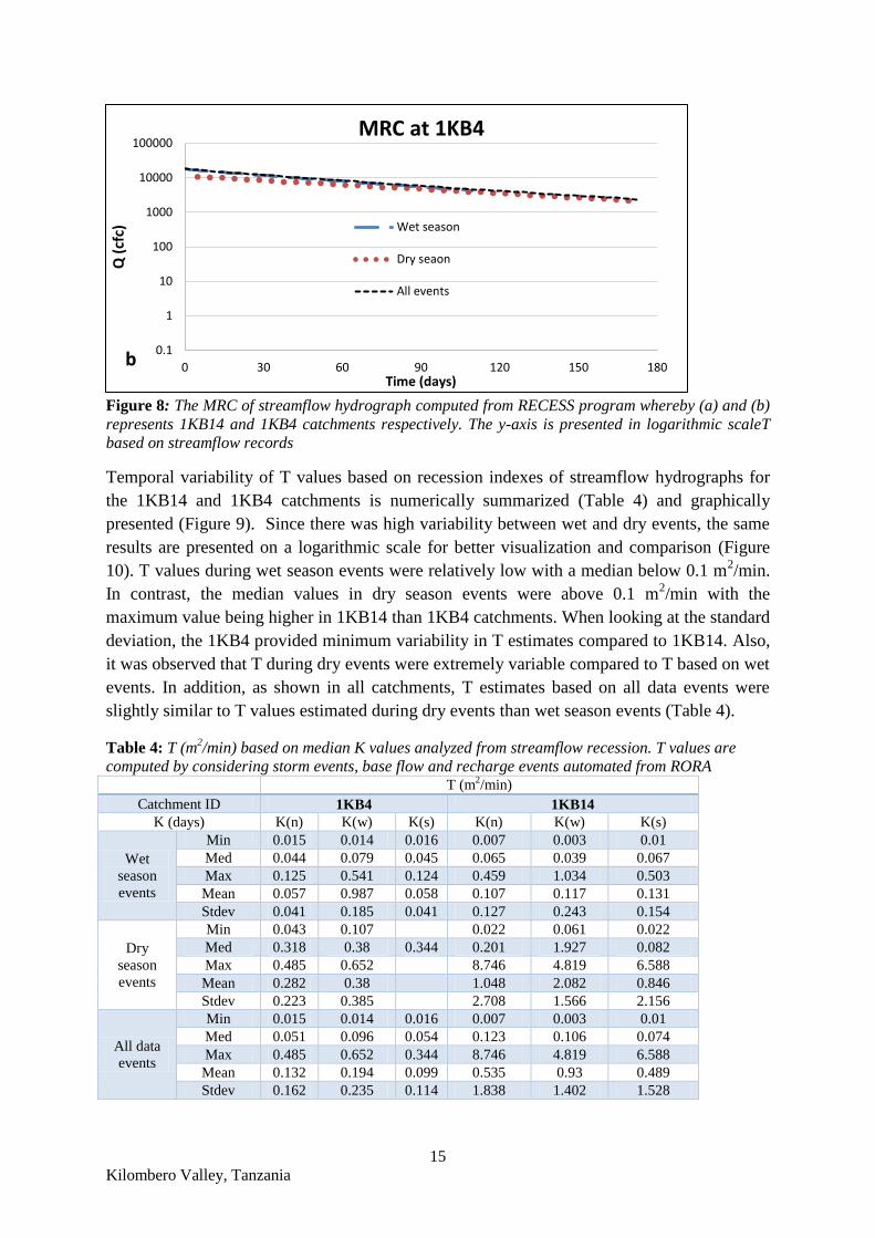
Figure 8: The MRC of streamflow hydrograph computed from RECESS program whereby (a) and (b)
represents 1KB14 and 1KB4 catchments respectively. The y-axis is presented in logarithmic
scale ........................................................................................................ Error! Bookmark not defined.
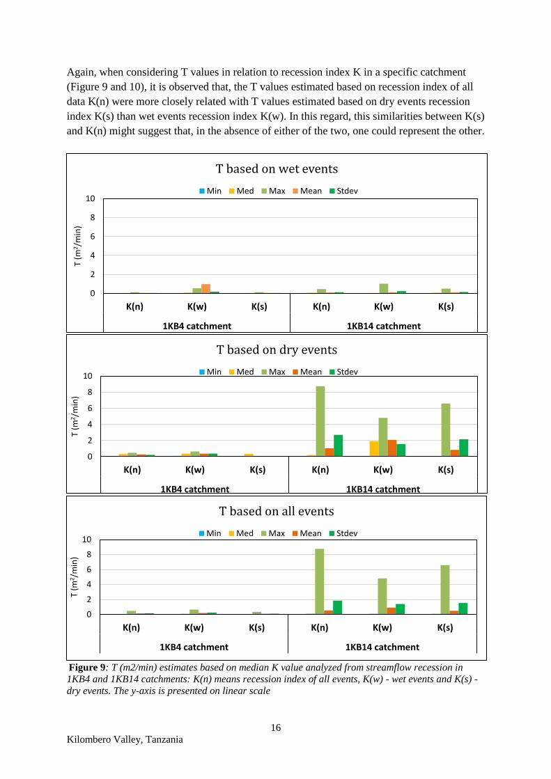
Figure 9: T (m2/min) estimates based on median K value analyzed from streamflow recession in 1KB4
and 1KB14 catchments: K(n) means recession index of all events, K(w) - wet events and K(s) -
dry events. The y-axis is presented on linear scale ................................. Error! Bookmark not defined.
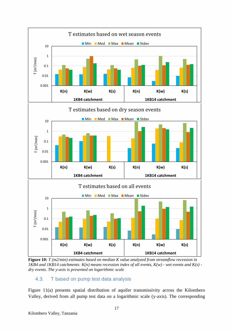
Figure 10: T (m2/min) estimates based on median K value analyzed from streamflow recession in
1KB4 and 1KB14 catchments: K(n) means recession index of all events, K(w) - wet events and
K(s) - dry events. The y-axis is presented on logarithmic scale .............. Error! Bookmark not defined.
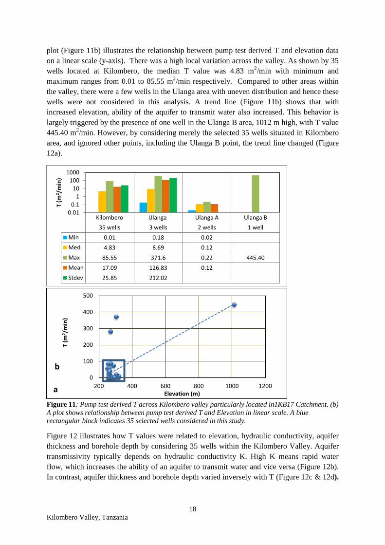
Figure 11: Pump test derived T across Kilombero valley particularly located in1KB17 Catchment. (b)
A plot shows relationship between pump test derived T and Elevation in linear scale. A blue
rectangular block indicates 35 selected wells considered in this study. . Error! Bookmark not defined.
Figure 12: T values related to elevation (a), hydraulic conductivity (b), aquifer thickness (c) and
borehole depth (d) within Kilombero valley by considering 35 selected wells located at 1KB17
Catchment. The y-axis is presented on linear scale. ............................... Error! Bookmark not defined.
Figure 13: T analysis based on elevation, aquifer thickness, depth and hydraulic conductivity
intervals within Kilombero Valley. The y-axis is presented in logarithmic scale. .............................. 20
Figure 14: Maps show spatial distribution of selected wells in Kilombero valley based on aquifer
transmissivity (m2/min), aquifer thickness (m), hydraulic conductivity (cm/sec), borehole depth
(m) and elevation (m) .............................................................................. Error! Bookmark not defined.
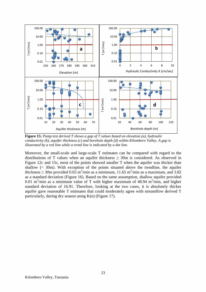
Figure 15: Pump test derived T shows a gap of T values based on elevation (a), hydraulic
conductivity (b), aquifer thickness (c) and borehole depth (d) within Kilombero Valley. A gap is
illustrated by a red line while a trend line is indicated by a dot line. ..... Error! Bookmark not defined.
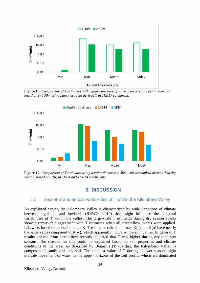
Figure 16: Comparison of T estimates with aquifer thickness greater than or equal (≥) to 30m and
less than (<) 30m using pump test data derived T in 1KB17 catchment. Error! Bookmark not defined.
Figure 17: Comparison of T estimates using aquifer thickness ≥ 30m with streamflow derived T in dry
season, based on K(n) in 1KB4 and 1KB14 catchments. .................................................................... 24
Figure A- 1: The MRC of streamflow hydrograph computed from RECESS program whereby (a) and
(b) represents 1KB14 and 1KB4 catchments respectively. Both axes are presented in linear scale .. 35

v Kilombero Valley, Tanzania
List of Tables
Table 1: Catchments characteristics within Kilombero Valley .................................................................. 10
Table 2: Wells within Kilombero Valley .................................................................................................... 11
Table 3: Summary of K (days) values estimated in this study. Wet season represents December
through April, dry season means May to November and all events stands for a whole year,
January to December. ......................................................................................................................... 12
Table 4: T (m2/min) based on median K values analyzed from streamflow recession. T values are
computed by considering storm events, base flow and recharge events automated from RORA
program............................................................................................................................................... 15
Table 5: Comparison of streamflow derived T and pump test derived T ................................................... 22
Table A- 1: Details of wells within Kilombero Valley ............................................................................... 34
Table A- 2: Summary of Aquifer transmissivity of 35 wells based on borehole characteristics ................ 35

vi Kilombero Valley, Tanzania

vii
Kilombero Valley, Tanzania
Acknowledgments
First and foremost, I would like to thank the Swedish Institute Study Scholarships (SI) for
funding my studies during the whole period of my study programme at Stockholm
University.
Also, I sincerely thank Steve Lyon, my main supervisor, and the head of Master‘s programme
in Hydrology, Hydrogeology, and Water Resources at the Department of Physical Geography
and Quaternary Geology. He provided very useful guidance and overall fruitful supervision
of my work. His general outline of this work, recommendations and feedback were great.
I extend my appreciation to Alexander Koutsouris, assistant supervisor, for data provision
and tremendous contributions to the introduction of this exciting topic.
Above all, I must express my very profound gratitude to my dearest father ―Mzee‖ Tuwa
Bakari, my brothers and sisters at home (Tanzania), and to my dear friend Dr. Mohammed for
providing me with unfailing support and continuous encouragement throughout my years of
study and through the process of writing this thesis. This accomplishment would not have
been possible without them.
Finally, I thank Allah, may He be glorified and exalted for the good health and patience
throughout my study and great favours and blessings that He has bestowed upon me
throughout my life. Alhamdulillah!

1
Kilombero Valley, Tanzania
1. INTRODUCTION
1.1. Background information
Besides the difficulties created by long-term climate change reducing the global amount of
natural water resources (Xu and Singh, 2004), increases in human population and correspond
water demand will bring about high demand of water resources in the various sectors
worldwide (Vörösmarty et al., 2000). This places extra pressure on groundwater resources
which are often considered relative climate resilient. In fact, as more than 1.5 billion people
globally rely on groundwater for various purposes (Alley et al., 2008), there is increased
global awareness and desire for assessing accurate ground water information in the last
decade (Soupios et al., 2007).
In developing countries like Tanzania, for example, insufficient provision of water supplies
raises the demand of groundwater utilization. Specifically, 30% of the total population and
42% of the population living in major cities depend on groundwater resource (Mato, 2002).
Access to water supplies in the villages and districts of Tanzania remains a big challenge, as
it requires great investments in initiating new water sources, modification and expansion of
water supply networks (URT, 2010). With respect to the Kilombero Valley in Tanzania,
where the projections of population growth and domestic water demand by 2035 are expected
to be the highest in the Rufiji Basin (WREM, 2013a), groundwater resources are used as an
additional source of water supply, and seen as a potential climate-stable future commodity.
Despite its potential usefulness, extensive studies on groundwater resources in the basin have
not been conducted, and therefore, it is difficult to obtain precise information on the basin‘s
water resources (Kashaigili, 2010; RBWO, 2010).
It is well known that the scarcity and inconvenient quality of data are the key sources
hampering modeling and management of water resources in developing countries (Brunner et
al., 2007; MacDonald et al., 2013; Van Camp et al., 2013; Singh, 2014). In such a way,
inadequate information, particularly hydraulic data often limit development of water
resources structures (Mendoza et al., 2003). Likewise, lack of extensive hydraulic data
reduces the capacity of the modelers to check for the precision of either semi or full
distributed hydrologic parameter models which need other data excluding streamflow.
Consequently, transmissivity and hydraulic conductivity are derived through model
calibrations (Brooks et al., 2004). Kashaigili (2012) showed that the quantity and quality of
groundwater data are the main challenges facing groundwater management in Tanzania. A
recent study by Lyon et al., (2014) also pointed out issues of data scarcity and quality in the
Kilombero Valley. Similarly, a Rufiji Basin report indicated problems of groundwater data
availability and insufficient aquifer information in the basin (RBWO, 2010). Moreover, as
requirement of drilling one borehole in Tanzania costs nearly 6000 US dollars (Baumann et
al., 2005), such observational techniques are expensive, and could be one of the reasons that
led to scanty of groundwater and aquifer information in the Kilombero Valley.
Traditionally, in hydrology, groundwater and surface water flows are considered to be related
(Alley et al., 2008; Dingman, 2008). According to Tallaksen (1995), streamflow has been
widely utilized in early studies due to its inherent connection with subsurface flow. This in
turn has led to advances in techniques using observations in surface water flows to estimate
groundwater factors. Under such conditions, streamflow recession techniques have been
useful in estimating aquifer hydraulic properties that are not easily measured, but are
important in the hydrologic responses of the catchments (Vannier et al., 2014; Oyarzún et al.,
2
Kilombero Valley, Tanzania
2014). Owing to that usefulness, numerous studies have applied recession techniques to
acquire groundwater and aquifer information. For example, Szilagyi et al., (1998) examined
recession flow to determine catchment-scale saturated hydraulic conductivity and average
aquifer depth. Mendoza et al., (2003) estimated basin-hydraulic parameters (transmissivity
and specific yield) of a semi-arid mountainous watershed based on recession flow analysis.
Huang et al., (2011) measured aquifer transmissivity in the Kaoping River basin based on
streamflow records. More recently, Lyon et al., (2014) determined characteristic drainage
timescale variability (storage coefficient) across the Kilombero Valley based on streamflow
recession. Vannier et al., (2014) estimated catchment-scale storage capacity and hydraulic
conductivity by means of streamflow recession analysis. Similarly, the arid basins study
conducted by Oyarzún et al., (2014) focused on recession flow analysis as a tool for
determining hydrogeological parameter such as aquifer thickness, hydraulic conductivity and
porosity.
As described by Tallaksen (1995), recession flow or low flow responses mean the part of
surface flow originating from groundwater or other delayed sources. Various techniques have
been employed in analyzing streamflow recession, and notable among them is the recession
curve displacement method developed by Rorabaugh (1964), commonly known as the
Rorabaugh Method (Rutledge 1998, 2007; Huang et al., 2011). The approach has been
manually used in several early studies (Rorabaugh, 1964; Daniel, 1976; Bevans, 1986).
However, the development of computers has enabled the researchers to automate the
procedures in objective way (Tallaksen, 1995). A recent approach proposed by Rutledge
(1993) based on the computer programs RECESS and RORA helped to simplify and
minimize subjectivity inherent in using manual methods (Rutledge, 2000; Yeh et al., 2015).
The program RECESS provides the master recession curve of streamflow recession data
while the program RORA automates the procedures of recession curve displacement to
estimate recharge for each storm event (Rutledge 1998, 2000). Among few examples of
researchers who applied the RECESS and RORA were Halford and Mayer (2000), Delin et
al., (2007), Huang et al., (2011), and Abo et al., (2015).
In general, multiple approaches such as stream-discharge recessions, groundwater
hydrograph recessions and aquifer test can be used to estimate hydraulic properties of the
aquifer (Halford and Mayer, 2000). What is typically required is full understanding of the
distributions of hydraulic parameters such as aquifer transmissivity to solve problems
concerning hydrogeology and related fields (Leven and Dietrich, 2006). By definition,
transmissivity (T) of an aquifer is described as the ability of an aquifer to transmit water with
the prevailing kinematic viscosity. It is mathematically equivalent to hydraulic conductivity
of the aquifer times saturated thickness of the aquifer (Heath, 1983). Compared to other
hydraulic properties, T is a key parameter in obtaining significant information in sub-surface
flow and contaminant transport modeling (Soupios et al., 2007). However, field-based
measurements of T (made using the pumping test) are often scarce and uncertain, with
variability of observed values characterized by numerous orders of magnitude compared to
other parameters (Jankovic et al., 2006; Mendoza et al., 2003).
In this regard, analytical approaches based on streamflow records to estimate the hydraulic
parameters offer a cost effective alternative approach due to high expenses of drilling
activities, particularly in developing countries (Zecharias and Brutseart 1988; Mendoza et al.,
2003). This is especially true in understanding sub-surface flow in the Kilombero Valley
given its large scale, and limited number of direct observations. In addition, it is applicable to
the Kilombero sub basin because, as stated by Huang et al., (2011), it is a useful approach
for basins where wells data are limited.
3
Kilombero Valley, Tanzania
1.2. Main Objective
Since the worth of an aquifer as a source of ground water depends mainly on its ability to
store and transmit water (Heath, 1983), this study aims to use an analytical approach adopted
by Huang et al., (2011) to determine aquifer transmissivity based on streamflow records in
Tanzania‘s Kilombero Valley. The study also considers pumping test data from selected
wells located within Kilombero for comparison. The T estimates derived from pumping test
and streamflow records are key parameters to provide insight about groundwater
development at a local and regional scale, respectively (Huang et al., 2011). Towards this
aim, the main study question is: What is aquifer transmissivity T in the Kilombero Valley?
Therefore, in order to answer a basic question, this study will investigate the following:
Seasonal variability of aquifer T within the Kilombero Valley
Spatial variability of aquifer T within the Kilombero
Comparison of large-scale streamflow derived T and small-scale pump tests derived T
Uncertainties associated with T estimation
2. THEORY OF THE ANALYTICAL APPROACH
Huang et al., (2011) applied an analytical approach derived from Rorabaugh theory (1964) to
estimate aquifer transmissivity based on streamflow hydrograph records in southern Taiwan.
The analytical approach was developed by combining instantaneous recharge theory, master
recession curve (MRC) and the recession-curve-displacement method. Since data scarcity is a
major problem facing Kilombero Valley (Lyon et al. 2014), Rorabaugh method was adopted
in this study to derive the aquifer parameter T from streamflow records and compared with T
derived from pumping test data.
2.1. Rorabaugh’s instantaneous recharge theory
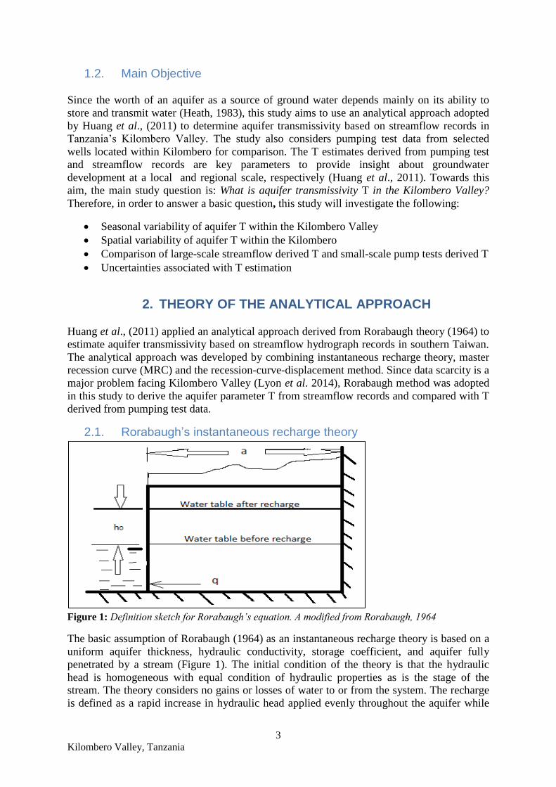
Figure 1: Definition sketch for Rorabaugh’s equation. A modified from Rorabaugh, 1964
The basic assumption of Rorabaugh (1964) as an instantaneous recharge theory is based on a
uniform aquifer thickness, hydraulic conductivity, storage coefficient, and aquifer fully
penetrated by a stream (Figure 1). The initial condition of the theory is that the hydraulic
head is homogeneous with equal condition of hydraulic properties as is the stage of the
stream. The theory considers no gains or losses of water to or from the system. The recharge
is defined as a rapid increase in hydraulic head applied evenly throughout the aquifer while

4
Kilombero Valley, Tanzania
stream stage remains constant. In addition, increase in hydraulic head due to recharge events
result in subsequent ground water discharge to the stream. The resulting ground water
discharge to the stream (q) which is commonly known as instantaneous recharge theoretical
model (Huang et al., 2011) is expressed in Eq. 1.
( )(
)
Eq. 1
Where q (m2) is the groundwater discharge (m
3) per unit stream length of one side (m), T
(m2/min) is aquifer transmissivity, (m) means instantaneous rise in water table, t (min) is
the time taken after h0, a (m) is the distance from stream to the groundwater divide and S is
aquifer storativity.
Daniel (1976); Johnston (1976) and Stricker (1983) expressed a quantity L as shown in Eq. 2
Eq. 2
Where L (m) is the length of the stream and A (m2) is drainage area of the basin. Further, a
constant C1 is computed using Eq. 3 where Q (m3) is total groundwater discharge.
Eq. 3
The relationship between T (m2/min) and S of the aquifer shown by exponential function
equation (Eq. 4), is the basis of the current study.
Eq. 4
By substituting Eq. 4 in the Rorabaugh and Simons (1966) baseflow model (Eq. 5), the T
value of the aquifer is estimated (Eq. 6).
( )
Eq. 5
Eq. 6
Where (m3) is a streamflow at the peak estimated during a time when the surface runoff
recession has started and (m3) is the baseflow recession (Huang et al., 2011).
2.2. Master Recession Curve (MRC) and Recession index (K)
Rutledge (1998) highlighted steps to develop a streamflow MRC and for the determination of
K using the program RECESS. The RECESS as a computerized program is based on
interactive procedures to calculate a best fit linear equation in order to obtain the MRC and
value of K. Despite the fact that, the program selects periods of continuous streamflow
5
Kilombero Valley, Tanzania
recession, the nearly linear segment selection is subjective. In the sense that, the program user
specifies which segments are sufficiently linear on the semi-log plot, for example, to be
analyzed. Once finished the selection of a segment, RECESS provides a mathematical
expression in the form as shown below:
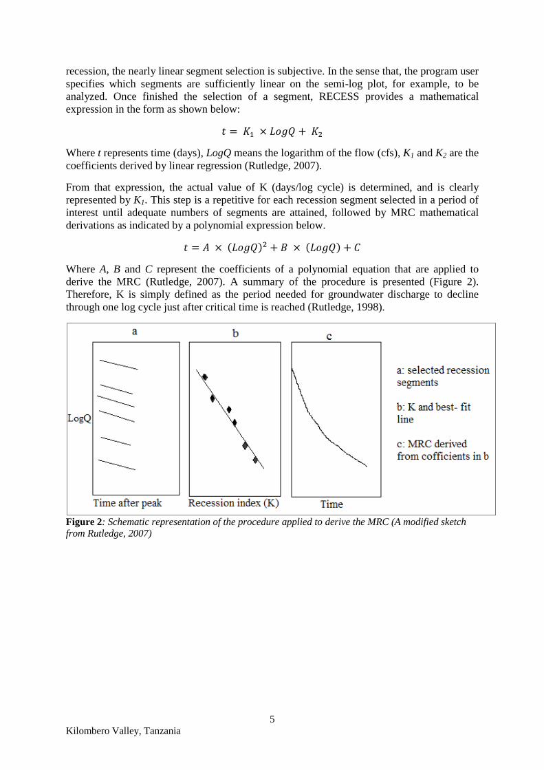
Where t represents time (days), LogQ means the logarithm of the flow (cfs), K1 and K2 are the
coefficients derived by linear regression (Rutledge, 2007).
From that expression, the actual value of K (days/log cycle) is determined, and is clearly
represented by K1. This step is a repetitive for each recession segment selected in a period of
interest until adequate numbers of segments are attained, followed by MRC mathematical
derivations as indicated by a polynomial expression below.
( ) ( )
Where A, B and C represent the coefficients of a polynomial equation that are applied to
derive the MRC (Rutledge, 2007). A summary of the procedure is presented (Figure 2).
Therefore, K is simply defined as the period needed for groundwater discharge to decline
through one log cycle just after critical time is reached (Rutledge, 1998).
Figure 2: Schematic representation of the procedure applied to derive the MRC (A modified sketch
from Rutledge, 2007)

6
Kilombero Valley, Tanzania
2.3. Recession curve-displacement method
Figure 3: Procedure for use the recession-curve displacement method. A modified sketch from
Bevans, 1986
According to Rutledge (1998), the procedures for recession curve-displacement method
(Figure 3) were developed by Bevans (1986) to estimate the total volume of ground water
recharge in a basin Q (cubic feet) during a single recharge event (Eq. 7). The method requires
K (day), critical time after a streamflow peak (day) (Eq. 8), and groundwater discharge at a
critical time extrapolated from pre-event (cfs) and post-event streamflow recessions
(cfs).
( )
Eq. 7
Eq. 8
Linsley et al., (1982) estimated the time of surface runoff (N) as a function of the drainage
area (A) using Eq. 9. The time of surface runoff is described as the time from a peak in
streamflow at the time when surface runoff ceases (Rutledge, 1997).

7
Kilombero Valley, Tanzania
Eq. 9
Where represents number of days after the peak in streamflow (rounded to the next larger
integer), and A means drainage area of the basin in square miles. These procedures are
automated using the RORA program (Rutledge, 2007), and calculated before the parameter T
is estimated (Huang et al., 2011). Eq. 9 which represents the requirement of antecedent
recession is considered as the basis for the applicability of RORA to a specific hydrologic
system (Rutledge, 2000). The program RORA assumes recharge events and streamflow peaks
are concurrent (Rutledge, 1998). On top of that, the RORA neglects explicitly the effects of
groundwater evapotranspiration (Rutledge, 2000).
3. METHODS
3.1. Study area description
3.1.1. Location
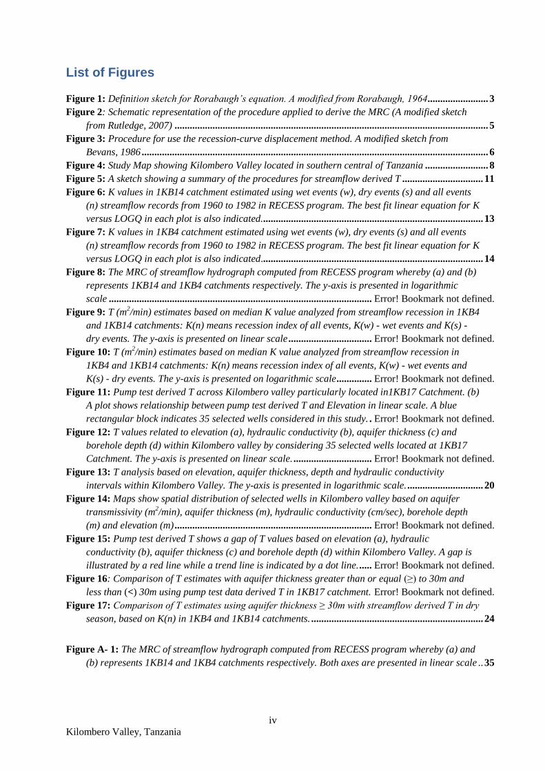
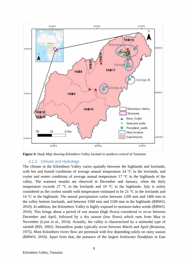
The Kilombero Valley (Figure 4) is geographically located between latitude 34°33′E and
37°20′E, and between longitude 7°39′S and 10°01′S (Lyon et al., 2014), south-central of
Tanzania. The valley lies on the lowland areas of the Rufiji Basin (RBWO, 2010). It is the
one among four sub-basin of the Rufiji River Basin, which encompasses 20% drainage area
and contributes 62% of total Rufiji Basin runoff (Mwalyosi, 1990). Its topographical
depression feature is estimated to range from the south-west to north-east of the valley. In the
north-west, Udzungwa Mountains rise abruptly to an elevation of 2000 m while in the south-
east, the ridge drops after several miles to form the steep Mahenge Mountain block which has
an average elevation between 900 m and 1500 m (Bonarius, 1975). These features create the
main catchment area, and thus, they are important to the hydrology of the valley (RBWO,
2010; WREM, 2013b). The stream monitoring point at 1KB17 thus defines the catchment
that covers nearly all of the Kilombero Valley area including the Kibasila wetland (WREM,
2013b).
8
Kilombero Valley, Tanzania
Figure 4: Study Map showing Kilombero Valley located in southern central of Tanzania
3.1.2. Climate and Hydrology
The climate in the Kilombero Valley varies spatially between the highlands and lowlands,
with hot and humid conditions of average annual temperature 24 °C in the lowlands, and
cooler and wetter conditions of average annual temperature 17 °C in the highlands of the
valley. The warmest months are observed in December and January, when the daily
temperature exceeds 27 °C in the lowlands and 19 °C in the highlands. July is solely
considered as the coolest month with temperature estimated to be 21 °C in the lowlands and
14 °C in the highlands. The annual precipitation varies between 1200 mm and 1400 mm in
the valley bottom lowlands, and between 1500 mm and 2100 mm in the highlands (RBWO,
2010). In addition, the Kilombero Valley is highly exposed to moisture‐laden winds (RBWO,
2010). This brings about a period of wet season (high flows) considered to occur between
December and April, followed by a dry season (low flows) which runs from May to
November (Lyon et al., 2014). Actually, the valley is characterized by a unimodal type of
rainfall (RIS, 2002). Streamflow peaks typically occur between March and April (Bonarius,
1975). Most Kilombero rivers flow are perennial with few depending solely on rainy season
(RBWO, 2010). Apart from that, the presence of the largest freshwater floodplain in East
9
Kilombero Valley, Tanzania
Africa contributes highly to the hydrology of the valley as it generates 2/3 of the annual
Rufiji river flow. The floodplain is considered as part of the Great Selous Ecosystem, an
important World Heritage Site (RIS, 2002).
3.1.3. Geology and Hydrogeology
The Kilombero Valley itself is a geologic feature resulted from tectonic movements which
cause folding, faulting and uplift of the earth‘s surface. According to Tanzania geology
settings, the valley is located within the Usagaran system of the Precambrian basement
complex rocks, an asymmetrical rift valley depression caused by Pliocene faultings. The
rocks composed in this system mostly are dominated with magmatic gneiss and acidic
granulites. The gneiss, rich in biotite is very easily weathered to fine grits and coarse sands;
the granulites are characterized by disintegration to stony material and fine grits. The parent
material consists of loamy gravelly in the transitional stage followed by loamy sand and
sandy loam soils (Bonarius, 1975; RBWO, 2010).
Groundwater recharge takes place at high altitude, mainly from rainwater infiltration
(Kashaigili, 2010) with smaller amount from rivers and lakes. The recharge is basically
controlled by climate, geology and geomorphology (RBWO, 2010). The infiltration
capacities in the Kilombero Valley are typically attributed to the presence of alluvial fans
(coarsely grained sands) and colluvial sand-flats or miombo plains soil types. Rapid to very
rapid infiltration rates with sufficient soil moisture availability occur in alluvial fans on the
valley bottom. The miombo plains allows very high infiltration rates with minimum soil
moisture availability (Bonarius, 1975).
3.2. Dataset
3.2.1. Hydrology data
The long-term daily streamflow and gage height data from 1KB4 and 1KB14 catchments
were considered in this study (Figure 4). These time series data that span 23 consecutive
years from 1960 to 1982 were derived from Rufiji Basin Water Board (RBWO). The data
quality was not good in general, as there were mismatch of peaks between gauge heights and
streamflow records in some periods. Also intermittents gaps in gage height records were
observed in 1KB4 catchment from 1973 to 1982.
3.2.2. Groundwater data
Since this study aims at comparison of T value estimates, pumping well data available in
1KB17 catchment were included (Figure 4). These data were already evaluated using the
Cooper–Jacob technique in which hydraulic parameters such as hydraulic conductivity and
transmissivity are estimated. Other information such as aquifer type, aquifer thickness and
borehole depth were also provided. The pump test activities were conducted in the dry season
between June and September, 2014.
3.2.3. Spatial dataset
A spatial dataset corresponding to basin drainage areas and wells locations derived from
RBWO was also considered. The general characteristics of catchments included in this study
are summarized in Table 1.

10
Kilombero Valley, Tanzania
Table 1: Catchments characteristics within Kilombero Valley
Catchment ID 1KB17 1KB4 1KB14
River Kilombero Kilombero Lumemo
Location Swero Ifwema Kiburubutu
Topographic Area (km2) 34230 18048 580
Stream length (km) 5916 2859 63
Average slope (%) 7 8 14
Landform Valley and alluvial plain (%) 22 8 0
Hill and mountain (%) 78 92 100
Source:Lyon et.al (2014)
3.3. Procedures for streamflow derived T
3.3.1. Determination of K and MRC
K was estimated from the program RECESS using all streamflow data (n) and the data were
divided into, wet (w) and dry (s) seasons. Streamflow (cfs) from 1960 to 1982 was
considered as the model input data required to generate the recession index and a master
recession curve in 1KB4 and 1B14 catchments. Initially, recession segments of streamflow
records were selected based on recession length and initial discharge. The segment selections
depended solely on days of antecedent recession (Eq. 9) which also represents groundwater
discharge (Rutledge, 2007). High variability among recession segments were observed, since
segment selection is subjective (Tallaksen, 1994). Therefore, a specific range regarding
segment lengths was defined in order to be consistent. Similarly, the RECESS program
produced a curve data as an output file whereby the MRC was created based on wet, dry and
all streamflow events for each catchment.
3.3.2. Estimation of mean aquifer T value
In order to automate recession curve displacement procedures (Figure 3) using the
computerized RORA program, the median K estimated from the program RECESS together
with streamflow records (cfs) and catchment area (sq.mile) were applied as model input
variables. The program RORA determined values of Qt, Q0, Q1 and Q2. Recharge events Q in
each storm, days of antecedent recession N, and critical time tc were also automated in the
program RORA using Eq. 6, 8 and 9, respectively. Nevertheless, not all events were used for
analysis. The most representative events were selected, and those events which did not meet
the specified conditions (predefined N, tc) were ignored. After having all necessary variables
from the program RORA, the next step was to quantify T value (Eq. 6). A manual procedure
to determine constant C1 was used by considering an aquifer half-width a calculated using
Eq. 2, h0 calculated from daily mean stream water table and recharge events Q. Finally, T
values were estimated as the product of C1 and Q0 divide by Qt. A summary of these
procedures are shown on the sketch below (Figure 5).
11
Kilombero Valley, Tanzania
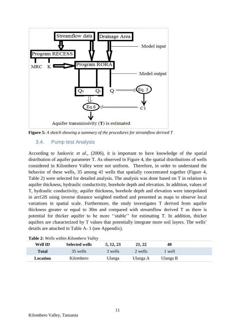
Figure 5: A sketch showing a summary of the procedures for streamflow derived T
3.4. Pump test Analysis
According to Jankovic et al., (2006), it is important to have knowledge of the spatial
distribution of aquifer parameter T. As observed in Figure 4, the spatial distributions of wells
considered in Kilombero Valley were not uniform. Therefore, in order to understand the
behavior of these wells, 35 among 41 wells that spatially concentrated together (Figure 4,
Table 2) were selected for detailed analysis. The analysis was done based on T in relation to
aquifer thickness, hydraulic conductivity, borehole depth and elevation. In addition, values of
T, hydraulic conductivity, aquifer thickness, borehole depth and elevation were interpolated
in arcGIS using inverse distance weighted method and presented as maps to observe local
variations in spatial scale. Furthermore, the study investigates T derived from aquifer
thickness greater or equal to 30m and compared with streamflow derived T as there is
potential for thicker aquifer to be more ‗‗stable‘‘ for estimating T. In addition, thicker
aquifers are characterized by T values that potentially integrate more soil layers. The wells‘
details are attached in Table A- 1 (see Appendix).
Table 2: Wells within Kilombero Valley
Well ID Selected wells 5, 12, 23 21, 22 40
Total 35 wells 3 wells 2 wells 1 well
Location Kilombero Ulanga Ulanga A Ulanga B
12
Kilombero Valley, Tanzania
4. RESULTS
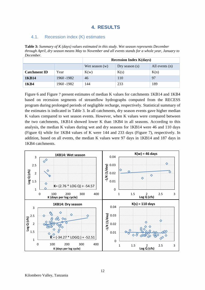
4.1. Recession index (K) estimates
Table 3: Summary of K (days) values estimated in this study. Wet season represents December
through April, dry season means May to November and all events stands for a whole year, January to
December.
Recession Index K(days)
Wet season (w) Dry season (s) All events (n)
Catchment ID Year K(w) K(s) K(n)
1KB14 1960 -1982 46 110 97
1KB4 1960 -1982 144 233 189
Figure 6 and Figure 7 present estimates of median K values for catchments 1KB14 and 1KB4
based on recession segments of streamflow hydrographs computed from the RECESS
program during prolonged periods of negligible recharge, respectively. Statistical summary of
the estimates is indicated in Table 3. In all catchments, dry season events gave higher median
K values compared to wet season events. However, when K values were compared between
the two catchments, 1KB14 showed lower K than 1KB4 in all seasons. According to this
analysis, the median K values during wet and dry seasons for 1KB14 were 46 and 110 days
(Figure 6) while for 1KB4 values of K were 144 and 233 days (Figure 7), respectively. In
addition, based on all events, the median K values were 97 days in 1KB14 and 187 days in
1KB4 catchments.
1
1.5
2
2.5
3
0 100 200 300 400
Log
Q (
cfs)
K (days per log cycle)
1KB14: Wet season
K= (2.76 * LOG Q) + -54.57 0
0.01
0.02
0.03
0.04
1 1.5 2 2.5 3
-1/K
(1
/day
)
Log Q (cfs)
K(w) = 46 days
1
1.5
2
2.5
3
0 100 200 300 400
Log
Q (
cfs)
K (days per log cycle)
1KB14: Dry season
K = (-34.27 * LOGQ ) + -52.51 0
0.01
0.02
0.03
0.04
1 1.5 2 2.5 3
-1/K
(1
/day
)
Log Q (cfs)
K(s) = 110 days
13
Kilombero Valley, Tanzania
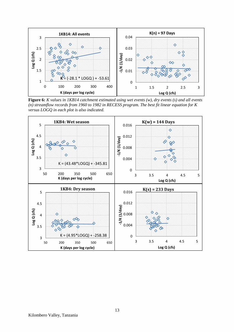
Figure 6: K values in 1KB14 catchment estimated using wet events (w), dry events (s) and all events
(n) streamflow records from 1960 to 1982 in RECESS program. The best fit linear equation for K
versus LOGQ in each plot is also indicated.
1
1.5
2
2.5
3
0 100 200 300 400
Log
Q (
cfs)
K (days per log cycle)
1KB14: All events
K = (-28.1 * LOGQ ) + -53.61 0
0.01
0.02
0.03
0.04
1 1.5 2 2.5 3
-1/K
(1
/day
)
Log Q (cfs)
K(n) = 97 Days
3
3.5
4
4.5
5
50 200 350 500 650
Log
Q (
cfs)
K (days per log cycle)
1KB4: Wet season
K = (43.48*LOGQ) + -345.81
0
0.004
0.008
0.012
0.016
3 3.5 4 4.5 5
-1/K
(1
/day
)
Log Q (cfs)
K(w) = 144 Days
3
3.5
4
4.5
5
50 200 350 500 650
Log
Q (
cfs)
K (days per log cycle)
1KB4: Dry season
K = (4.95*LOGQ) + -258.38 0
0.004
0.008
0.012
0.016
3 3.5 4 4.5 5
-1/K
(1
/day
)
Log Q (cfs)
K(s) = 233 Days
14
Kilombero Valley, Tanzania
Figure 7: K values in 1KB4 catchment estimated using wet events (w), dry events (s) and all events
(n) streamflow records from 1960 to 1982 in RECESS program. The best fit linear equation for K
versus LOGQ in each plot is also indicated.
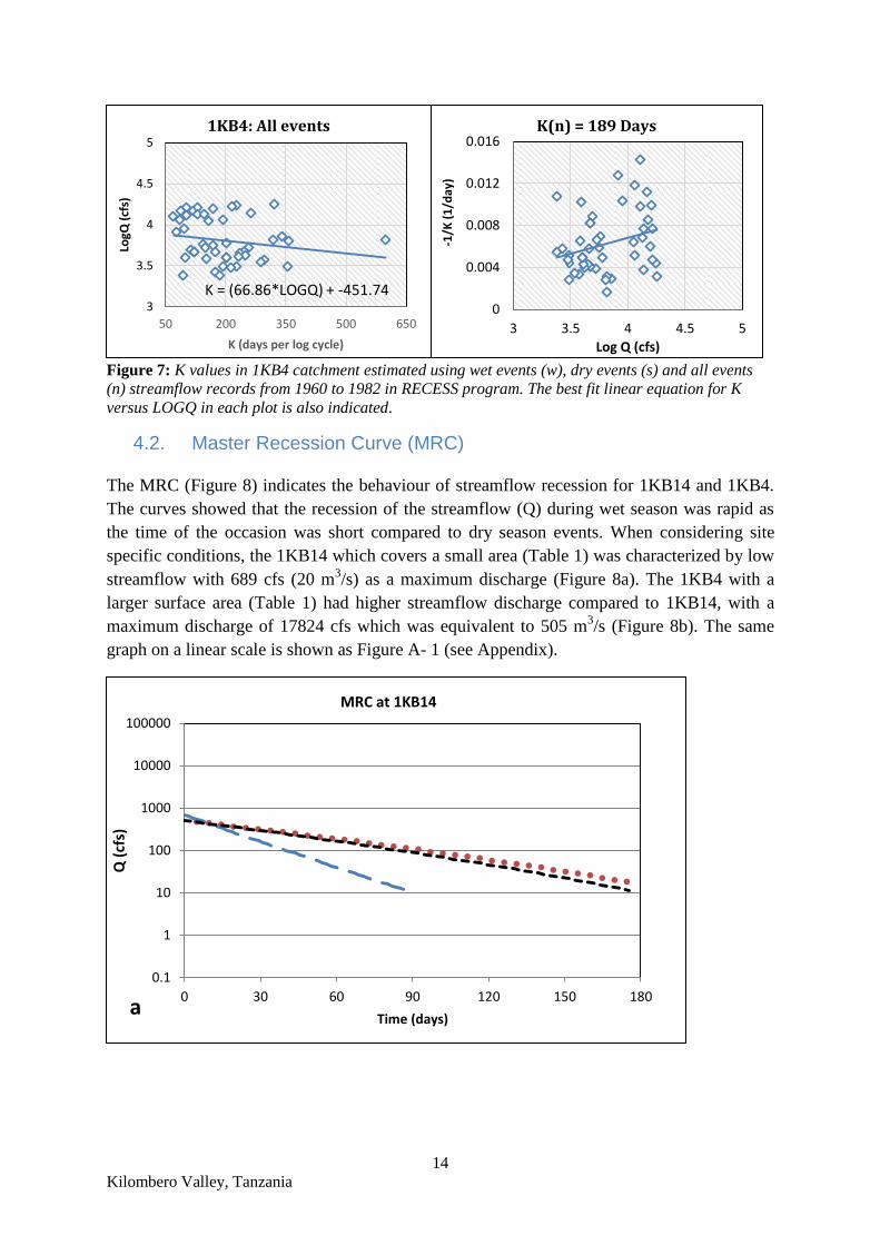
4.2. Master Recession Curve (MRC)
The MRC (Figure 8) indicates the behaviour of streamflow recession for 1KB14 and 1KB4.
The curves showed that the recession of the streamflow (Q) during wet season was rapid as
the time of the occasion was short compared to dry season events. When considering site
specific conditions, the 1KB14 which covers a small area (Table 1) was characterized by low
streamflow with 689 cfs (20 m3/s) as a maximum discharge (Figure 8a). The 1KB4 with a
larger surface area (Table 1) had higher streamflow discharge compared to 1KB14, with a
maximum discharge of 17824 cfs which was equivalent to 505 m3/s (Figure 8b). The same
graph on a linear scale is shown as Figure A- 1 (see Appendix).
3
3.5
4
4.5
5
50 200 350 500 650
LogQ
(cf
s)
K (days per log cycle)
1KB4: All events
K = (66.86*LOGQ) + -451.74 0
0.004
0.008
0.012
0.016
3 3.5 4 4.5 5
-1/K
(1
/day
)
Log Q (cfs)
K(n) = 189 Days
0.1
1
10
100
1000
10000
100000
0 30 60 90 120 150 180
Q (
cfs)
Time (days)
MRC at 1KB14
a
15
Kilombero Valley, Tanzania
Figure 8: The MRC of streamflow hydrograph computed from RECESS program whereby (a) and (b)
represents 1KB14 and 1KB4 catchments respectively. The y-axis is presented in logarithmic scaleT
based on streamflow records
Temporal variability of T values based on recession indexes of streamflow hydrographs for
the 1KB14 and 1KB4 catchments is numerically summarized (Table 4) and graphically
presented (Figure 9). Since there was high variability between wet and dry events, the same
results are presented on a logarithmic scale for better visualization and comparison (Figure
10). T values during wet season events were relatively low with a median below 0.1 m2/min.
In contrast, the median values in dry season events were above 0.1 m2/min with the
maximum value being higher in 1KB14 than 1KB4 catchments. When looking at the standard
deviation, the 1KB4 provided minimum variability in T estimates compared to 1KB14. Also,
it was observed that T during dry events were extremely variable compared to T based on wet
events. In addition, as shown in all catchments, T estimates based on all data events were
slightly similar to T values estimated during dry events than wet season events (Table 4).
Table 4: T (m2/min) based on median K values analyzed from streamflow recession. T values are
computed by considering storm events, base flow and recharge events automated from RORA
T (m
2/min)
Catchment ID 1KB4 1KB14
K (days) K(n) K(w) K(s) K(n) K(w) K(s)
Wet
season
events
Min 0.015 0.014 0.016 0.007 0.003 0.01
Med 0.044 0.079 0.045 0.065 0.039 0.067
Max 0.125 0.541 0.124 0.459 1.034 0.503
Mean 0.057 0.987 0.058 0.107 0.117 0.131
Stdev 0.041 0.185 0.041 0.127 0.243 0.154
Dry
season
events
Min 0.043 0.107
0.022 0.061 0.022
Med 0.318 0.38 0.344 0.201 1.927 0.082
Max 0.485 0.652
8.746 4.819 6.588
Mean 0.282 0.38
1.048 2.082 0.846
Stdev 0.223 0.385
2.708 1.566 2.156
All data
events
Min 0.015 0.014 0.016 0.007 0.003 0.01
Med 0.051 0.096 0.054 0.123 0.106 0.074
Max 0.485 0.652 0.344 8.746 4.819 6.588
Mean 0.132 0.194 0.099 0.535 0.93 0.489
Stdev 0.162 0.235 0.114 1.838 1.402 1.528
0.1
1
10
100
1000
10000
100000
0 30 60 90 120 150 180
Q (
cfc)
Time (days)
MRC at 1KB4
Wet season
Dry seaon
All events
b
16
Kilombero Valley, Tanzania
Again, when considering T values in relation to recession index K in a specific catchment
(Figure 9 and 10), it is observed that, the T values estimated based on recession index of all
data K(n) were more closely related with T values estimated based on dry events recession
index K(s) than wet events recession index K(w). In this regard, this similarities between K(s)
and K(n) might suggest that, in the absence of either of the two, one could represent the other.
Figure 9: T (m2/min) estimates based on median K value analyzed from streamflow recession in
1KB4 and 1KB14 catchments: K(n) means recession index of all events, K(w) - wet events and K(s) -
dry events. The y-axis is presented on linear scale
0
2
4
6
8
10
K(n) K(w) K(s) K(n) K(w) K(s)
1KB4 catchment 1KB14 catchment
T (m
2/m
in)
T based on wet events
Min Med Max Mean Stdev
0
2
4
6
8
10
K(n) K(w) K(s) K(n) K(w) K(s)
1KB4 catchment 1KB14 catchment
T (m
2 /m
in)
T based on dry events
Min Med Max Mean Stdev
0
2
4
6
8
10
K(n) K(w) K(s) K(n) K(w) K(s)
1KB4 catchment 1KB14 catchment
T (m
2 /m
in)
T based on all events
Min Med Max Mean Stdev
17
Kilombero Valley, Tanzania
Figure 10: T (m2/min) estimates based on median K value analyzed from streamflow recession in
1KB4 and 1KB14 catchments: K(n) means recession index of all events, K(w) - wet events and K(s) -
dry events. The y-axis is presented on logarithmic scale
4.3. T based on pump test data analysis
Figure 11(a) presents spatial distribution of aquifer transmissivity across the Kilombero
Valley, derived from all pump test data on a logarithmic scale (y-axis). The corresponding
0.001
0.01
0.1
1
10
K(n) K(w) K(s) K(n) K(w) K(s)
1KB4 catchment 1KB14 catchment
T (m
2/m
in)
T estimates based on wet season events
Min Med Max Mean Stdev
0.001
0.01
0.1
1
10
K(n) K(w) K(s) K(n) K(w) K(s)
1KB4 catchment 1KB14 catchment
T (m
2 /m
in)
T estimates based on dry season events
Min Med Max Mean Stdev
0.001
0.01
0.1
1
10
K(n) K(w) K(s) K(n) K(w) K(s)
1KB4 catchment 1KB14 catchment
T (m
2/m
in)
T estimates based on all events
Min Med Max Mean Stdev
18
Kilombero Valley, Tanzania
plot (Figure 11b) illustrates the relationship between pump test derived T and elevation data
on a linear scale (y-axis). There was a high local variation across the valley. As shown by 35
wells located at Kilombero, the median T value was 4.83 m2/min with minimum and
maximum ranges from 0.01 to 85.55 m2/min respectively. Compared to other areas within
the valley, there were a few wells in the Ulanga area with uneven distribution and hence these
wells were not considered in this analysis. A trend line (Figure 11b) shows that with
increased elevation, ability of the aquifer to transmit water also increased. This behavior is
largely triggered by the presence of one well in the Ulanga B area, 1012 m high, with T value
445.40 m2/min. However, by considering merely the selected 35 wells situated in Kilombero
area, and ignored other points, including the Ulanga B point, the trend line changed (Figure
12a).
Figure 11: Pump test derived T across Kilombero valley particularly located in1KB17 Catchment. (b)
A plot shows relationship between pump test derived T and Elevation in linear scale. A blue
rectangular block indicates 35 selected wells considered in this study.
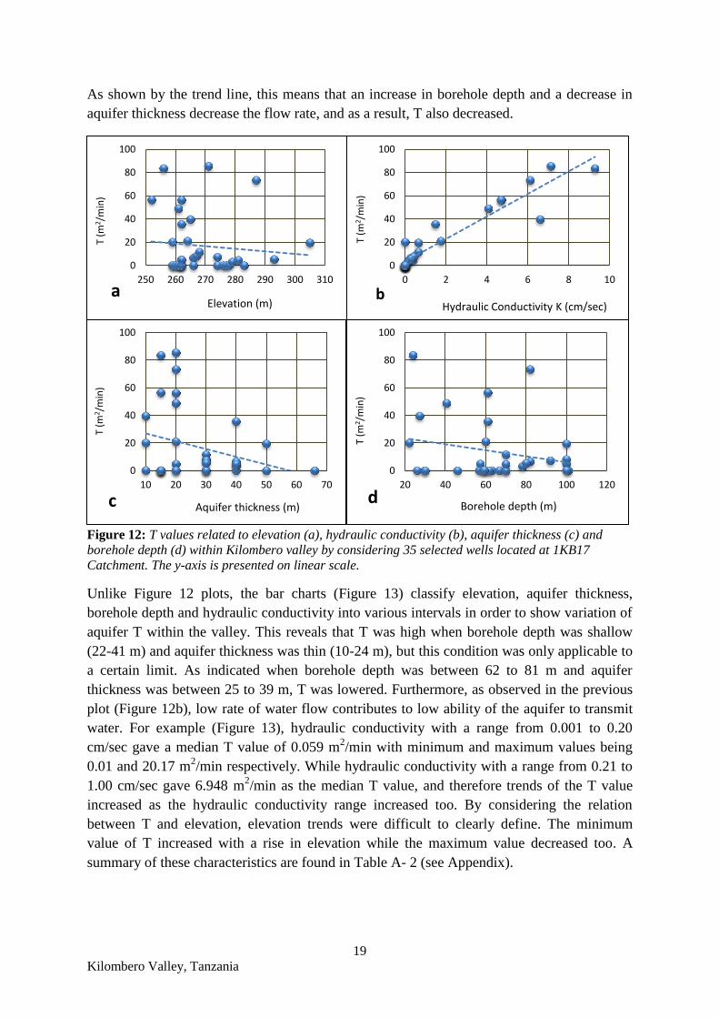
Figure 12 illustrates how T values were related to elevation, hydraulic conductivity, aquifer
thickness and borehole depth by considering 35 wells within the Kilombero Valley. Aquifer
transmissivity typically depends on hydraulic conductivity K. High K means rapid water
flow, which increases the ability of an aquifer to transmit water and vice versa (Figure 12b).
In contrast, aquifer thickness and borehole depth varied inversely with T (Figure 12c & 12d).
Kilombero Ulanga Ulanga A Ulanga B
35 wells 3 wells 2 wells 1 well
Min 0.01 0.18 0.02
Med 4.83 8.69 0.12
Max 85.55 371.6 0.22 445.40
Mean 17.09 126.83 0.12
Stdev 25.85 212.02
0.010.1
110
1001000
T (m
2 /m
in)
0
100
200
300
400
500
200 400 600 800 1000 1200
T (m
2/m
in)
Elevation (m)
b
a
19
Kilombero Valley, Tanzania
As shown by the trend line, this means that an increase in borehole depth and a decrease in
aquifer thickness decrease the flow rate, and as a result, T also decreased.
Figure 12: T values related to elevation (a), hydraulic conductivity (b), aquifer thickness (c) and
borehole depth (d) within Kilombero valley by considering 35 selected wells located at 1KB17
Catchment. The y-axis is presented on linear scale.
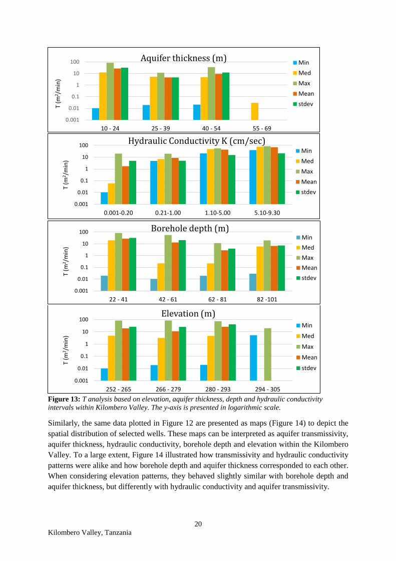
Unlike Figure 12 plots, the bar charts (Figure 13) classify elevation, aquifer thickness,
borehole depth and hydraulic conductivity into various intervals in order to show variation of
aquifer T within the valley. This reveals that T was high when borehole depth was shallow
(22-41 m) and aquifer thickness was thin (10-24 m), but this condition was only applicable to
a certain limit. As indicated when borehole depth was between 62 to 81 m and aquifer
thickness was between 25 to 39 m, T was lowered. Furthermore, as observed in the previous
plot (Figure 12b), low rate of water flow contributes to low ability of the aquifer to transmit
water. For example (Figure 13), hydraulic conductivity with a range from 0.001 to 0.20
cm/sec gave a median T value of 0.059 m2/min with minimum and maximum values being
0.01 and 20.17 m2/min respectively. While hydraulic conductivity with a range from 0.21 to
1.00 cm/sec gave 6.948 m2/min as the median T value, and therefore trends of the T value
increased as the hydraulic conductivity range increased too. By considering the relation
between T and elevation, elevation trends were difficult to clearly define. The minimum
value of T increased with a rise in elevation while the maximum value decreased too. A
summary of these characteristics are found in Table A- 2 (see Appendix).
0
20
40
60
80
100
250 260 270 280 290 300 310
T (m
2 /m
in)
Elevation (m) a
0
20
40
60
80
100
0 2 4 6 8 10
T (m
2 /m
in)
Hydraulic Conductivity K (cm/sec) b
0
20
40
60
80
100
10 20 30 40 50 60 70
T (m
2 /m
in)
Aquifer thickness (m) c
0
20
40
60
80
100
20 40 60 80 100 120
T (m
2 /m
in)
Borehole depth (m) d
20
Kilombero Valley, Tanzania
Figure 13: T analysis based on elevation, aquifer thickness, depth and hydraulic conductivity
intervals within Kilombero Valley. The y-axis is presented in logarithmic scale.
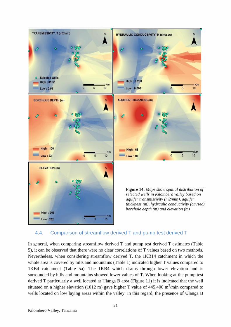
Similarly, the same data plotted in Figure 12 are presented as maps (Figure 14) to depict the
spatial distribution of selected wells. These maps can be interpreted as aquifer transmissivity,
aquifer thickness, hydraulic conductivity, borehole depth and elevation within the Kilombero
Valley. To a large extent, Figure 14 illustrated how transmissivity and hydraulic conductivity
patterns were alike and how borehole depth and aquifer thickness corresponded to each other.
When considering elevation patterns, they behaved slightly similar with borehole depth and
aquifer thickness, but differently with hydraulic conductivity and aquifer transmissivity.
0.001
0.01
0.1
1
10
100
10 - 24 25 - 39 40 - 54 55 - 69
T (m
2/m
in)
Aquifer thickness (m) Min
Med
Max
Mean
stdev
0.001
0.01
0.1
1
10
100
0.001-0.20 0.21-1.00 1.10-5.00 5.10-9.30
T (m
2/m
in)
Hydraulic Conductivity K (cm/sec) Min
Med
Max
Mean
stdev
0.001
0.01
0.1
1
10
100
22 - 41 42 - 61 62 - 81 82 -101
T (m
2/m
in)
Borehole depth (m) Min
Med
Max
Mean
stdev
0.001
0.01
0.1
1
10
100
252 - 265 266 - 279 280 - 293 294 - 305
T (m
2/m
in)
Elevation (m) Min
Med
Max
Mean
stdev
21
Kilombero Valley, Tanzania
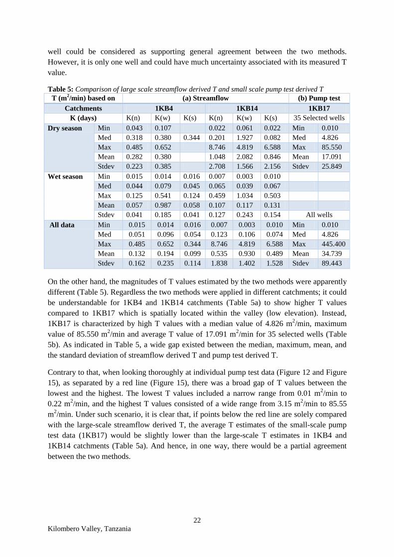
4.4. Comparison of streamflow derived T and pump test derived T
In general, when comparing streamflow derived T and pump test derived T estimates (Table
5), it can be observed that there were no clear correlations of T values based on two methods.
Nevertheless, when considering streamflow derived T, the 1KB14 catchment in which the
whole area is covered by hills and mountains (Table 1) indicated higher T values compared to
1KB4 catchment (Table 5a). The 1KB4 which drains through lower elevation and is
surrounded by hills and mountains showed lower values of T. When looking at the pump test
derived T particularly a well located at Ulanga B area (Figure 11) it is indicated that the well
situated on a higher elevation (1012 m) gave higher T value of 445.400 m2/min compared to
wells located on low laying areas within the valley. In this regard, the presence of Ulanga B
Figure 14: Maps show spatial distribution of
selected wells in Kilombero valley based on
aquifer transmissivity (m2/min), aquifer
thickness (m), hydraulic conductivity (cm/sec),
borehole depth (m) and elevation (m)
22
Kilombero Valley, Tanzania
well could be considered as supporting general agreement between the two methods.
However, it is only one well and could have much uncertainty associated with its measured T
value.
Table 5: Comparison of large scale streamflow derived T and small scale pump test derived T
T (m2/min) based on (a) Streamflow (b) Pump test
Catchments 1KB4 1KB14 1KB17
K (days) K(n) K(w) K(s) K(n) K(w) K(s) 35 Selected wells
Dry season Min 0.043 0.107 0.022 0.061 0.022 Min 0.010
Med 0.318 0.380 0.344 0.201 1.927 0.082 Med 4.826
Max 0.485 0.652 8.746 4.819 6.588 Max 85.550
Mean 0.282 0.380 1.048 2.082 0.846 Mean 17.091
Stdev 0.223 0.385 2.708 1.566 2.156 Stdev 25.849
Wet season Min 0.015 0.014 0.016 0.007 0.003 0.010
Med 0.044 0.079 0.045 0.065 0.039 0.067
Max 0.125 0.541 0.124 0.459 1.034 0.503
Mean 0.057 0.987 0.058 0.107 0.117 0.131
Stdev 0.041 0.185 0.041 0.127 0.243 0.154 All wells
All data Min 0.015 0.014 0.016 0.007 0.003 0.010 Min 0.010
Med 0.051 0.096 0.054 0.123 0.106 0.074 Med 4.826
Max 0.485 0.652 0.344 8.746 4.819 6.588 Max 445.400
Mean 0.132 0.194 0.099 0.535 0.930 0.489 Mean 34.739
Stdev 0.162 0.235 0.114 1.838 1.402 1.528 Stdev 89.443
On the other hand, the magnitudes of T values estimated by the two methods were apparently
different (Table 5). Regardless the two methods were applied in different catchments; it could
be understandable for 1KB4 and 1KB14 catchments (Table 5a) to show higher T values
compared to 1KB17 which is spatially located within the valley (low elevation). Instead,
1KB17 is characterized by high T values with a median value of 4.826 m2/min, maximum
value of 85.550 m2/min and average T value of 17.091 m
2/min for 35 selected wells (Table
5b). As indicated in Table 5, a wide gap existed between the median, maximum, mean, and
the standard deviation of streamflow derived T and pump test derived T.
Contrary to that, when looking thoroughly at individual pump test data (Figure 12 and Figure
15), as separated by a red line (Figure 15), there was a broad gap of T values between the
lowest and the highest. The lowest T values included a narrow range from 0.01 m2/min to
0.22 m2/min, and the highest T values consisted of a wide range from 3.15 m
2/min to 85.55
m2/min. Under such scenario, it is clear that, if points below the red line are solely compared
with the large-scale streamflow derived T, the average T estimates of the small-scale pump
test data (1KB17) would be slightly lower than the large-scale T estimates in 1KB4 and
1KB14 catchments (Table 5a). And hence, in one way, there would be a partial agreement
between the two methods.
23
Kilombero Valley, Tanzania
Figure 15: Pump test derived T shows a gap of T values based on elevation (a), hydraulic
conductivity (b), aquifer thickness (c) and borehole depth (d) within Kilombero Valley. A gap is
illustrated by a red line while a trend line is indicated by a dot line.
Moreover, the small-scale and large-scale T estimates can be compared with regard to the
distributions of T values when an aquifer thickness ≥ 30m is considered. As observed in
Figure 12c and 15c, most of the points showed smaller T when the aquifer was thicker than
shallow (< 30m). With exception of the points situated above the trendline, the aquifer
thickness ≥ 30m provided 0.02 m2/min as a minimum, 11.65 m
2/min as a maximum, and 3.82
as a standard deviation (Figure 16). Based on the same assumption, shallow aquifer provided
0.01 m2/min as a minimum value of T with higher maximum of 48.94 m
2/min, and higher
standard deviation of 16.91. Therefore, looking at the two cases, it is absolutely thicker
aquifer gave reasonable T estimates that could moderately agree with streamflow derived T
particularly, during dry season using K(n) (Figure 17).
0.01
0.10
1.00
10.00
100.00
250 260 270 280 290 300 310
T (m
2 /m
in)
Elevation (m)
a
0.01
0.10
1.00
10.00
100.00
0 2 4 6 8 10
T (m
2 /m
in)
Hydraulic Conductivity K (cm/sec)
b
0.01
0.10
1.00
10.00
100.00
10 20 30 40 50 60 70
T (m
2 /m
in)
Aquifer thickness (m)
c
0.01
0.10
1.00
10.00
100.00
20 40 60 80 100 120
T (m
2 /m
in)
Borehole depth (m)
d
24
Kilombero Valley, Tanzania
Figure 16: Comparison of T estimates with aquifer thickness greater than or equal (≥) to 30m and
less than (<) 30m using pump test data derived T in 1KB17 catchment.
Figure 17: Comparison of T estimates using aquifer thickness ≥ 30m with streamflow derived T in dry
season, based on K(n) in 1KB4 and 1KB14 catchments.
5. DISCUSSION
5.1. Seasonal and annual variabilities of T within the Kilombero Valley
As explained earlier, the Kilombero Valley is characterized by wide variations of climate
between highlands and lowlands (RBWO, 2010) that might influence the temporal
variabilities of T within the valley. The large-scale T estimates during dry season events
showed remarkable agreement with T estimates when all streamflow events were applied.
Likewise, based on recession index K, T estimates calculated from K(s) and K(n) have nearly
the same values compared to K(w), which apparently indicated lower T values. In general, T
results derived from streamflow records indicated that T was higher during dry than wet
seasons. The reasons for this could be explained based on soil properties and climate
conditions of the area. As described by Bonarius (1975) that, the Kilombero Valley is
composed of sandy and clay soil. The smallest value of T during the wet season might
indicate movement of water in the upper horizons of the soil profile which are dominated
0.01
0.10
1.00
10.00
100.00
Min Max Mean Stdev
T (m
2 /m
in)
Aquifer thickness (m)
< 30m ≥ 30m
0.01
0.10
1.00
10.00
100.00
Min Max Mean Stdev
T (m
2 /m
in)
Aquifer thickness 1KB14 1KB4
25
Kilombero Valley, Tanzania
with clay soil. On the other hand, during the dry season as the water movement reaches
deeper profile layers and the sand soil becomes more dominant, the T became higher due to
high porous nature of the sandy soil. However, this is in the case when the soil layers are
homogeneous throughout. In non-homogeneous soil, the case could be different. This later
issue could indicate the differences between the well derived T and the streamflow derived T,
but needs more consideration.
Besides that, when relating the average small-scale T values estimated from thicker aquifers
(≥ 30m) with soil properties, it is sufficient to assume that, the thicker aquifer that showed
lower T values are possibly dominated by clay soil, and the shallow aquifer that indicated
higher T values are possibly dominated by unconsolidated sandy soil. However, it should be
noted that, if the aquifer thickness is interpreted as equal to soil profile depths, this case could
probably contradict the above discussion.
5.2. Spatial variability of aquifer T within the Kilombero Valley
Considering the spatial variability of T within Kilombero Valley, an agreement was found
between streamflow recessions and catchment topography. The 1KB14 catchment with an
average slope of 14%, which is higher value compared to other catchments, has smaller K
values than 1KB4 with an average slope of only 8% (Table 1 and Table 3). Consequently,
these topographic characteristics of catchment scale gave higher estimates of T values in
1KB14 than 1KB4 based on streamflow records (Figure 9 and Figure 10). This means that,
the aquifer with larger slope drains rapidly (Brutsaert, 1994) and hence, influences the high
capacity of the aquifer to transmit water. In addition, as presented by Brutsaert (1994), the
subsurface outflow from a hill slope is influenced by pressure gradients due to the inclination
of the water table with reference to the underlying restrictive layer, and magnitude of the
slope due to gravity. This proves how the 1KB14 with high slope could have higher T values
compared to 1KB4 and 1KB17 catchments. The lower variability of T in large-scale
estimates could probably accounted by drainage area. The 1KB4 with larger drainage area
indicated minimum T variability compared to 1KB14 which has a smaller drainage area
(Figure 9 and Figure 10).
By looking at the spatial distribution of wells (Figure 14), one would anticipate that there is
uniformity between aquifer T and elevation trends. However, for the Kilombero Valley
particularly 1KB17 wells, the case was obviously not true. Interestingly, the distributions of
individual wells based on aquifer T in relation to the elevation data provided no clear
description about spatial variability of T in the valley. Both wells located on either high or
low elevation showed mixed trends (Figure 15a), except for the one well located in Ulanga B
(Figure 11). This means that, there are multiple factors affecting the spatial variability of T in
the valley, and therefore more research should be conducted. Nevertheless, the higher
variability of T (25.85 standard deviation) exhibited by the small-scale pump test data, could
certainly a potential indicator describing aquifer inhomogeneity within the Kilombero Valley
or, might be due to a limited number of measurements on a local scale. A point of
inhomogeneity was also emphasized by Foster and Chilton (2003) that a broad variability of
aquifer saturated thickness leads to higher variability of aquifer T. This is a fact, and it is
typically correlated with pump test data presented in this study.
26
Kilombero Valley, Tanzania
5.3. Comparison of streamflow derived T and pump test derived T
In general, comparison between the T derived from streamflow (large-scale T estimate) and
pump test (small-scale T estimate) can be accounted based on either, time-space variations
within the Kilombero Valley, or other factors. Spatially, the measurements of T obtained
from pump test data at 1KB17 catchment showed imprecise values with a high degree of
variation ranging from 0.01 m2/min as a minimum, to 85.55 m
2/min as maximum (Table 5b).
The T derived from the analytical approach at 1KB4 and 1KB14 catchments showed lower
consistent values compared to the direct field measurements of T, with minimum values
greater than 0.01 m2/min and maximum values less than 10 m
2/min (Table 5a). This defines
how the T derived from streamflow records and that from pump test data are inconsistent
with each other. In spite of inconsistency between them, a large-scale T estimate can solely
be compared with a small-scale T estimate derived from thicker aquifer, as both of them gave
reasonable lower T estimates that partly agree with each other (Figure 17). It would be better
to compare T derived from pump test at 1KB17 with T derived from the analytical approach
on the same catchment. But, as important information required using the analytical approach
in 1KB17 was missing, the analysis was excluded. Further, given the 1KB17, like 1KB4 and
1KB14, integrate large regions of land and drains both the upland and valley regions, it is not
necessarily a given that the analytical method applied at this scale would match exactly with
the well derived T values.
Based on geomorphology, the 1KB17 which lies on the valley bottom should provide low
estimates followed by 1KB4 and 1KB14. Notwithstanding, the small-scale T estimates
generated in 1KB17, were characterized by higher values with greater deviation than
streamflow derived T in 1KB4 and 1KB14 catchments. This characteristic is supported by
findings of Jankovic et al., (2006) and Mendoza et al., (2003) studies about uncertainty and
high variability of parameter T regarding to field-based measurements. And, it reveals how
difficulties it is in comparing T derived from the analytical approach with the field
measurement method in the Kilombero Valley. In addition, the difference in the period of
records between streamflow (1960-1982) and pump test (2014) dataset might contribute to
the variability of T estimates. This is typically true, as described by Halford and Mayer
(2000), more frequently the recession-curve-displacement method tends to be untrustworthy,
due to failure of underlying analytical groundwater flow model to interpret the contributing
aquifer. Such an interpretation would be consistent with the general findings of Lyon et al.,
(2014) where seasonality and scale greatly impacted the linearity of the hydrologic response
across the Kilombero Valley.
5.4. Comparison with other study findings
Since, both hydraulic conductivity (Ks) and T, are important hydraulic parameters in the
hydrological cycle and modeling perspective in a catchment (Davis et al., 1999; Sobieraj et
al., 2001; Brooks et al., 2004; Soupios et al., 2007), the disparity between the large-scale
derived T and small-scale derived T can also be discussed on a basis of Ks findings from
other study. With reference to Brooks et al., (2004) views on hillslope-scale experiment about
lateral Ks, they found that a reason for the small-scale Ks to have lower values than the
calibrated lateral Ks were due to stumbling blocks implicit in the small-scale sampling
27
Kilombero Valley, Tanzania
technique. Hopmans et al., (2002) investigation of soil hydraulic properties using small-scale
and large-scale estimates demonstrated that dealing with the scale disparity by looking at
spatial or temporal scale variability, was something to consider. This is because, space and
time differences in the soil develop uncertainties when large and small scales are subjected to
changes. Also, a huge nonlinearity characterized by flow and transport processes in
geophysics and large-scale vadose zone hydrology was another issue to take into account
(Hopmans et al., 2002). However, they argued that a proper knowledge of large-scale flow
processes in non-homogeneous soils, could likely be achieved when there is suitable
technologies for scale appropriate measurement. Davis et al., (1999) employed different
measurement techniques to determine the sensitivity of a catchment model to soil hydraulic
properties. They found that different methods may have little or higher estimate relevant for a
specific soil layer. Therefore, it is unreasonable to have one conclusion on the performance of
all measurement techniques. They suggested that, in order to acquire accurate model results,
it is better to check for the accuracy of a particular method on a basis of a site-specific soil
characteristic.
Moreover, the concept of sample size and macropores distribution at catchment scale
(Mohanty et al., 1994; Davis et al., 1999; Sobieraj et al., 2001; Brooks et al., 2004), could
perhaps reflect the limitation of why the large-scale and small-scale T estimates were
typically not comparable in this study. A main reason speculated by Brooks et al., (2004) was
an inadequate number of sample size inhibited a real average of Ks in small-scale
measurements. This case is obviously valid for T estimates based on pump test data applied
in this study. Fewer observation points were not sufficient to represent the actual average
estimates, and hence affect the interpretation of hydrological model in the catchment scale.
Even though, as clearly pointed out by Brooks et al., (2004), despite the appropriate number
of samples are considered, the small-scale may not depict the same values with the large-
scale measurements. In addition, as explained by Davis et al., (1999), macropores as
structural features of soil are potential of the soil hydraulic properties and their determined
values have a potential effect on the scale of measurement. This is true for small-scale
sampling techniques whereby the presence of large macropores or weak structures in the soil
hinder quantification (Brooks et al., 2004). Simultaneously, lack of information on how
macropores are connected in a large-scale measurement (Beven and Germann, 1982), adds
more difficulties for the two methods to be comparable (Brooks et al., 2004). Therefore, in
connection with this study, these findings could reasonably prove that, it is impossible for T
values derived from small-scale and those from large-scale measurements to be statistically
the same.
5.5. Uncertainties associated with T estimation
Although no uncertainty tests were performed to measure the reliability of T values
estimated, still, the results obtained from this study were associated with uncertainties. This is
because no model is error free as mathematical computations are often not similar to the real
catchment characteristics (Vogel and Kroll, 1992). The quality of the data itself was
somewhat imprecise. Presence of intermittent gaps in gage height records and mismatch of
peaks created questions in particular over the measurement techniques used. Moreover, as the
RORA (Rutledge, 2000; Delin et al., 2007) and RECESS (Rutledge, 1998) require the long-
28
Kilombero Valley, Tanzania
term continuous streamflow data with high quality, the inconvenient quality of data adds
more uncertainty of the results. Lack of abundant information such as water table and pump
test data in other catchments limited a full understanding of the study site. The temporal
variability between pump test and streamflow data might contribute to the uncertainty due to
impact of anthropogenic and climate changes that occur over time. Different measurement
techniques could also raise uncertainty, as small-scale pump tests derived T is a point
measurement, while streamflow derived T is a non-point measurement.
Based on scale of measurement, the program RORA needs drainage area exceeding 1 sq. mile
and less than 500 sq. mile (Rutledge, 2000). But, the 1KB4 catchment covers an area of
18048 km2 (6968 sq. mile) which is out of the RORA limitation. As specified by Rutledge
(2000), although that limitation is not universal and is subjective relying on hydrologic
setting, the effect of large areas create non-uniformity of storm events and lead to mix
multiple hydrogeologic settings. Also, the assumption that streamflow recession depends
solely on groundwater discharge, and exclude other sources such as river bank storage and
wetlands (Rutledge, 2000) might bring doubt about the model applicability in the Kilombero
Valley since some parts of 1KB4 catchment is covered by wetland.
6. CONCLUSION
The problem of data scarcity in an aquifer transmissivity (T) can be dealt with by using
different modeling approaches to derive the aquifer T .This can serve various purposes in
water resources management at local and regional scale. In this study, Rorabaugh model was
applied as an analytical approach to derive large-scale aquifer T based on streamflow records
in the Kilombero Valley. To ensure the accuracy, the modeled T estimates were compared
with T derived from pump test records. Based on specific objectives of the study, the
following were observed:
The close correlations between T estimates based on dry events and all data events
suggests that it is appropriate to apply dry events to calculate annual (all data events) T in
the absence of wet events in the Kilombero Valley.
Soil behavior during wet and dry seasons influenced temporal changes of T estimates
derived from large-scale streamflow records. Likewise, for small-scale measurements,
since thicker (≥ 30m) and shallow (< 30m) aquifers are characterized by lower and higher
T values, they are probably dominated by clay and unconsolidated sandy soil,
respectively.
As surface and subsurface flow characteristics vary in time, the temporal changes of
dataset records between streamflow (1960-1982) and pump tests (2014) reduce the
accuracy of the results, and may significantly influence uncertainty when comparing T
estimates.
Average basin slope appears to have contributed to the spatial variability of the large-
scale T estimates in the valley. The 1KB14 catchment with steep slope showed higher T
29
Kilombero Valley, Tanzania
values than the gentle slope 1KB4 catchment. However, no significant relation was found
between the elevations of individual wells location and T derived from pump test of
wells. The higher T estimates derived from the small-scale measurement could either
infer high heterogeneity of aquifer within the valley specifically, 1KB17 catchment,
difficulty of measurement technique, and limited number of measurements.
General results of streamflow derived T and pump test derived T suggest difficulties in
comparing the analytical approach with field-based measurement data in the Kilombero
Valley. The large-scale T estimates derived from the analytical approach indicates
significantly lower values with smaller variation than the small-scale estimates, hence,
typically incomparable.
With reference to other findings, possible reasons for large-scale T estimates to be lower
than small-scale estimates may be due to the limitation inherent in the RORA method
within the valley, seasonality and scale of measurements, and improper quality of data.
However, when considering T derived from field-based measurement is convenient, it is
obvious to conclude that, the analytical approach based on streamflow records
underestimate the T values in the Kilombero Valley.
In this regard, this study can be considered as a basis for future work. Therefore, further
study, including multiple approaches should be subjected to the area to find out the
appropriate approach which will provide reliable theoretical T values in comparison with
field-based measurement data. For a detailed analysis, the study should also consider missing
information such as pump test wells, streamflow, water table, and gauge height data are
included.
30
Kilombero Valley, Tanzania
References
Abo, R. K., and Merkel, B. J (2015) Investigation of the potential surface–groundwater relationship
using automated base-flow separation techniques and recession curve analysis in Al Zerba region of
Aleppo, Syria. Arab J Geosci (2015) 8:10543–10563 DOI 10.1007/s12517-015-1965-6
Alley, W. M., Healy, R. W., LaBaugh, J. W., and Reilly, T. E (2002) Flow and Storage in
Groundwater Systems www.sciencemag.org SCIENCE VOL 296, 1985 (2002)
DOI:10.1126/science.1067123.
Baumann, E., Ball, P., and Beyene, A (2005) Rationalization of Drilling Operations in Tanzania.
Review of the borehole drilling sector in Tanzania
Bevans, H. E (1986) Estimating stream-aquifer interactions in coal areas of eastern Kansas by using
streamflow records. Selected papers in the Hydrologic Sciences. U.S. Geological Survey Water-
Supply Paper 2290, pages 51-64. http://pubs.usgs.gov/wsp/wsp2290/pdf/wsp_2290.pdf
Beven, K., and Germann, P (1982) Macropores and water flow in soils, Water Resour. Res., 18(5),
1311– 1325.
Bonarius, H. (1975) Physical Properties of Soils in the Kilombero Valley (Tanzania), Agency for
Technical Cooperation, Ltd. (GTZ). Eschborn, Germany
Brooks, E. S., Boll, J., and McDaniel, P. A (2004) A hillslope-scale experiment to measure lateral
saturated hydraulic conductivity, Water Resour. Res., 40, W04208, doi: 10.1029/2003WR002858
Brunner, P., Hendricks Franssen, H. –J., Kgotlhang, L., Bauer-Gottwein, P., Kinzelbach, W (2007)
How can remote sensing contribute in groundwater modeling? Hydrogeology Journal (2007) 15: 5–
18. DOI 10.1007/s10040-006-0127-z
Brutsaert, W (1994) The unit response of groundwater outflow from a hillslope. Water Resources
Research, Vol. 30, NO. 10, Pages 2756 – 2763. Paper number 94WR01396. 0043 – 1397/94/94WR-
01396$05.00
Daniel, J. F (1976) Estimating Groundwater Evapotranspiration from Streamflow Records. Water
Resources Research, Vol. 12, No. 3, pages 360-364
Davis, H. S., Vertessy, A. R., and Silberstein, P. R (1999) The sensitivity of a catchment model to soil
hydraulic properties obtained by using different measurement techniques. Hydrol. Process. 13, 677-
688
Delin, G. N., Healy, R. W., Lorenz, D. L., and Nimmo, J. R (2007) Comparison of local- to regional-
scale estimates of ground-water recharge in Minnesota, USA. Journal of Hydrology (2007) 334, 231–
249 doi:10.1016/j.jhydrol.2006.10.010
Dingman, S. L (2008) Physical Hydrology. Second edition, 10-digit ISBN 1-57766-561-9, 13-digit
ISBN 978-1-57766-561-8. Pages 342-353
Foster, S. S. D and Chilton, P. J (2003) Groundwater: the processes and global significance of aquifer
degradation. The Royal Society Vol. 358, 1957–1972, DOI:10.1098/rstb.2003.1380
Halford, K. J and Mayer, G. C (2000) Problems Associated with Estimating Groundwater Discharge
and Recharge from Stream-Discharge Records. Groundwater Vol. 38, no. 3:331-342
Heath, R. C (1983) Basic of Ground Water Hydrology, U.S. Geological Survey Water-Supply Paper
2220
31
Kilombero Valley, Tanzania
Hopmans, W. J., Nielsen, R. D., and Bristow, L. K (2002) How Useful are Small-Scale Soil
Hydraulic Property Measurements for Large-Scale Vadose Zone Modeling? Environmental
Mechanics: Water, Mass and Energy Transfer in the Biosphere, vol. 129, pp. 247 – 258, AGU,
Washington, D. C
Huang, Y. P., Kung, W. J. and Lee, C. H (2010) Estimating aquifer transmissivity in a basin based on
stream hydrograph records using an analytical approach, Environ Earth Sci (2011) 63:461-468, DOI
10.1007/s12665-010-0712-2
Johnston, R. H (1976) Relation of ground water to surface water in four small basins of the Delaware
Coastal Plain, Delaware. U.S Geological Survey Report of Investigations, vol 24, 19 p
Jankovic´, I., Fiori, A., Suribhatla, R. and Dagan, G (2006) Identification of Heterogeneous Aquifer
Transmissivity Using an AE-Based Method. Vol. 44, No. 1—GROUND WATER—January–February
2006 (pages 62–71) doi: 10.1111/j.1745-6584.2005.00083.x
Kashigili, J. J (2012) Groundwater Availability and Use in Sub-Saharan Africa, A Review of 15
Countries, Chapter 13, Tanzania. Pages 207 – 228. Published by International Water Management
Institute
Kashaigili, J. J (2010) Assessment of groundwater availability and its current and potential use and
impacts in Tanzania – Final Report, Report prepared for the International Water Management Institute
(IWM1)
Leven, C. and Dietrich, P (2005) What information can we get from pumping tests?-comparing
pumping test configurations using sensitivity coefficients. Journal of Hydrology 319 (2006) 199–215,
doi:10.1016/j.jhydrol.2005.06.030
Linsley, R. K., Jr., Kohler, M.A., and Paulhus, J. L. H., (1982), Hydrology for engineers (3d ed.):
New York, McGraw-Hill, 508 p.
Lyon, S. W., Koutsouris, A., Scheibler, F., Jarsjö, J., Mbanguka, R., Tumbo, M., Robert, K. K.,
Sharma, A. N., and van der Velde, Y (2014) Interpreting characteristic drainage timescale variability
across Kilombero Valley, Tanzania. DOI: 10.1002/hyp.10304
MacDonald, A. M., Taylor, R. G., and Bonsor, H. C (2013) Groundwater in Africa – is there
sufficient water to support the intensification of agriculture frm ‗‗Land Grabs‘‘? In Allan A et al (eds.)
2013 Hand book of land and water grabs in Africa pp 376 – 383 Alliance for a Green Revolution in
Africa (http://www.agra-alliance.org/)
Mato, R. R. A. M (2002) Groundwater Pollution in Urban Dar es Salaam, Tanzania. Assessing
Vulnerability and Protection Priorities
Mendoza, G. F., Steenhuis, T. S., Walter, M. T., and Parlange, J.-Y (2003) Estimating basin-wide
hydraulic parameters of a semi-arid mountainous watershed by recession-flow analysis. Journal of
Hydrology 279 (2003) 57–69, doi: 10.1016/S0022-1694(03)00174-4
Mohanty, B. P., Kanwar, R. S., and Everts, C. J (1994) Comparison of Saturated Hydraulic
Conductivity Measurement Methods for a Glacial-Till Soil. Published in Soil Sci. Soc. Am. J. 58:672-
677 (1994).
Mwalyosi, R. B. B (1990) Resource Potentials of the Rufiji River Basin, Tanzania Vol. 19, No. 1, pp.
16-20

32
Kilombero Valley, Tanzania
Oyarzún, R., Godoy, R., Núñez, J., Fairley, J. P., Oyarzún, J., Maturana, H., and Freixas, G (2014)
Recession flow analysis as a suitable tool for hydrogeological parameter determination in steep, arid
basins. Journal of Arid Environments 105 (2014) 1-11,
http://dx.doi.org/10.1016/j.jaridenv.2014.02.012
Rorabaugh, M. I (1964) Estimating changes in bank storage and ground-water contribution to
streamflow. Int Assoc Sci Hydrol Publ 63:432-441
Rorabaugh, M. I., and Simons, W. D (1966) Exploration of the methods relating ground water to
surface water, Columbia River basin-second phase. US Geological Survey Open file Report
RBWO, Rufiji Basin Water Office (2010) Water Resources Availability Assessment, Volume 1
RIS - Ramsar Information Sheet (2002) Information Sheet on Ramsar Wetlands
https://rsis.ramsar.org/RISapp/files/RISrep/TZ1173RIS.pdf Accessed 11 April 2014
Rutledge, A.T (1993), Computer programs for describing the recession of ground-water discharge
and for estimating mean ground-water recharge and discharge from streamflow records: U.S.
Geological Survey Water-Resources Investigations Report 93-4121
Rutledge, A.T (1998) Computer Programs for Describing the Recession of Ground-Water Discharge
and for Estimating Mean Ground-Water Recharge and Discharge from Streamflow Records—Update,
U.S. Geological Survey Water-Resources Investigations Report 98-4148
Rutledge, A.T., (2000) Considerations for use of the RORA program to estimate ground-water
recharge from streamflow records: U.S. Geological Survey Open-File Report 00-156, 44 p
Rutledge, A.T (2007) Update on the Use of the RORA Program for Recharge Estimation, Vol. 45,
No. 3- GROUND WATER – May – June 2007 pages 374-382
Singh, A (2014) Groundwater resources management through the applications of simulation
modeling: A review. Science of the Total Environment 499 (2014) 414–423
DOI.org/10.1016/j.scitotenv.2014.05.048
Sobieraj, J. A., Elsenbeer, H., and Vertessy, R. A (2001) Pedotransfer functions for estimating
saturated hydraulic conductivity: implications for modeling storm flow generation. Journal of
Hydrology 251 (2001) 202-220
Soupios, P. M., Kouli, M., Vallianatos, F., Vafidis, A. and Stavroulakis, G (2007) Estimation of
aquifer hydraulic parameters from surficial geophysical methods: A case study of Keritis Basin in
Chania (Crete – Greece) Journal of Hydrology (2007) 338, 122– 131,
doi:10.1016/j.jhydrol.2007.02.028
Stricker, V. A (1983) Base flow of streams in the outcrop area of Southeastern sand aquifer: South
Carolina, Georgia, Alabama, and Mississippi. U.S Geological Survey Water-Resources Investigations
Report 83-4106
Szilagyi, J., Parlange, M. B., and Albertson, J. D (1998) Recession flow analysis for aquifer
parameter determination Paper number 98WR01009. 0043-1397/98/98WR-01009509.00, 1851 - 1857
Tallaksen, L. M (1994). A review of baseflow recession analysis, Journal of hydrology 165 (1995)
349-370
URT – The United Republic of Tanzania (2010) NATIONAL STRATEGY FOR GROWTH AND
REDUCTION OF POVERTY II NSGRP II. MINISTRY OF FINANCE AND ECONOMIC AFFAIRS

33
Kilombero Valley, Tanzania
http://www.international.gc.ca/development-developpement/assets/pdfs/countries-pays/NATIONAL-
STRATEGY-FOR-GROWTH-AND-REDUCTION-OF-POVERTY-TANZANIA.PDF
Van Camp, M., Mjemah, I. C., Al Farrah, N., and Walraevens, K (2013) Modeling approaches and
strategies for data-scarce aquifers: example of the Dar es Salaam aquifer in Tanzania. Hydrogeology
Journal (2013) 21: 341–356, DOI 10.1007/s10040-012-0908-5
Vannier, O., Braud, I., and Anquetin, S (2014) Regional estimation of catchment-scale soil properties
by means of streamflow recession analysis for use in distributed hydrological models. Hydrol.
Process. 28, 6276–6291 (2014), DOI:10.1002/hyp.10101
Vogel, R. M., and Kroll, C. N (1992), Regional geohydrologic-geomorphic relationships for the
estimation of low-flow statistics. Water Resour. Res., 28(9), 2451–2458, DOI:10.1029/92WR01007
Vörösmarty, C. J., Green, P., Salisbury, J. and Lammers, R (2000) Global water resources:
vulnerability from climate change and population growth. Science, 289, 284–288
WREM International Inc. (2013a) Rufiji Basin IWRMD Plan Draft Interim Report II Volume 2:
Water Management Options based on National Development Policies and Sectoral Plans
WREM International Inc. (2013b) Rufiji Basin IWRMD Plan Draft Interim Report II Volume 1,
Climate and hydrologic Modeling and Assessments developed for the Ministry of Water, United
Republic of
Tanzania
Yeh, H. –F., Kung, W. –J., Lee, J. –W., and Lee, C. –H (2015) Hydrograph separation for evaluating
streamflow recession characteristics in Taiwan, Sustain. Environ. Res., 25(2), 103-114
Xu, C. –Y., and Singh, V. P (2004) Review on Regional Water Resources Assessment Models under
Stationary and Changing Climate. Water Resources Management 18: 591-612
Zecharias, Y. B. and Brutsaert, W (1988) The influence of basin morphology on groundwater
outflow.
Water Resour. Res. (10), 1645–1650
Front cover image source
https://rsis.ramsar.org/ris/1173 downloaded on 12 April 2016 and
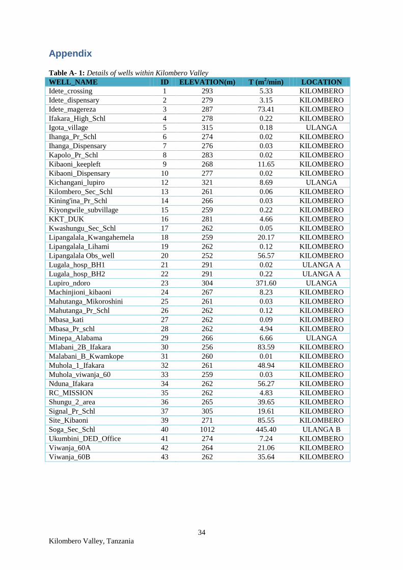
34
Kilombero Valley, Tanzania
Appendix
Table A- 1: Details of wells within Kilombero Valley
WELL_NAME ID ELEVATION(m) T (m2/min) LOCATION
Idete_crossing 1 293 5.33 KILOMBERO
Idete_dispensary 2 279 3.15 KILOMBERO
Idete_magereza 3 287 73.41 KILOMBERO
Ifakara_High_Schl 4 278 0.22 KILOMBERO
Igota_village 5 315 0.18 ULANGA
Ihanga_Pr_Schl 6 274 0.02 KILOMBERO
Ihanga_Dispensary 7 276 0.03 KILOMBERO
Kapolo_Pr_Schl 8 283 0.02 KILOMBERO
Kibaoni_keepleft 9 268 11.65 KILOMBERO
Kibaoni_Dispensary 10 277 0.02 KILOMBERO
Kichangani_lupiro 12 321 8.69 ULANGA
Kilombero_Sec_Schl 13 261 0.06 KILOMBERO
Kining'ina_Pr_Schl 14 266 0.03 KILOMBERO
Kiyongwile_subvillage 15 259 0.22 KILOMBERO
KKT_DUK 16 281 4.66 KILOMBERO
Kwashungu_Sec_Schl 17 262 0.05 KILOMBERO
Lipangalala_Kwangahemela 18 259 20.17 KILOMBERO
Lipangalala_Lihami 19 262 0.12 KILOMBERO
Lipangalala Obs_well 20 252 56.57 KILOMBERO
Lugala_hosp_BH1 21 291 0.02 ULANGA A
Lugala_hosp_BH2 22 291 0.22 ULANGA A
Lupiro_ndoro 23 304 371.60 ULANGA
Machinjioni_kibaoni 24 267 8.23 KILOMBERO
Mahutanga_Mikoroshini 25 261 0.03 KILOMBERO
Mahutanga_Pr_Schl 26 262 0.12 KILOMBERO
Mbasa_kati 27 262 0.09 KILOMBERO
Mbasa_Pr_schl 28 262 4.94 KILOMBERO
Minepa_Alabama 29 266 6.66 ULANGA
Mlabani_2B_Ifakara 30 256 83.59 KILOMBERO
Malabani_B_Kwamkope 31 260 0.01 KILOMBERO
Muhola_1_Ifakara 32 261 48.94 KILOMBERO
Muhola_viwanja_60 33 259 0.03 KILOMBERO
Nduna_Ifakara 34 262 56.27 KILOMBERO
RC_MISSION 35 262 4.83 KILOMBERO
Shungu_2_area 36 265 39.65 KILOMBERO
Signal_Pr_Schl 37 305 19.61 KILOMBERO
Site_Kibaoni 39 271 85.55 KILOMBERO
Soga_Sec_Schl 40 1012 445.40 ULANGA B
Ukumbini_DED_Office 41 274 7.24 KILOMBERO
Viwanja_60A 42 264 21.06 KILOMBERO
Viwanja_60B 43 262 35.64 KILOMBERO
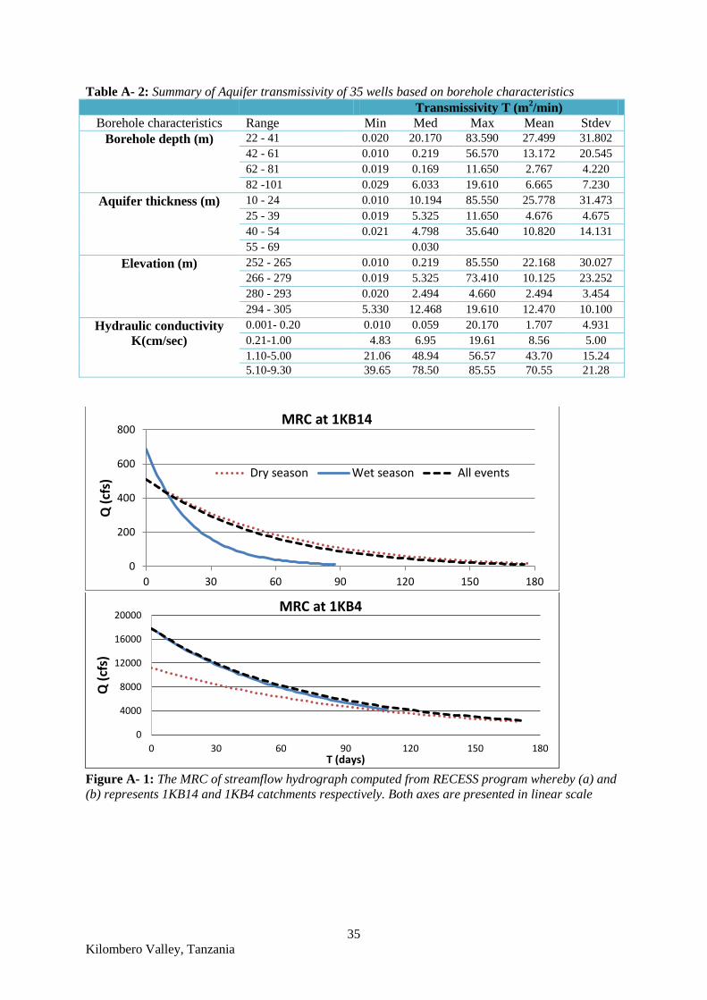
35
Kilombero Valley, Tanzania
Table A- 2: Summary of Aquifer transmissivity of 35 wells based on borehole characteristics
Transmissivity T (m2/min)
Borehole characteristics Range Min Med Max Mean Stdev
Borehole depth (m) 22 - 41 0.020 20.170 83.590 27.499 31.802
42 - 61 0.010 0.219 56.570 13.172 20.545
62 - 81 0.019 0.169 11.650 2.767 4.220
82 -101 0.029 6.033 19.610 6.665 7.230
Aquifer thickness (m) 10 - 24 0.010 10.194 85.550 25.778 31.473
25 - 39 0.019 5.325 11.650 4.676 4.675
40 - 54 0.021 4.798 35.640 10.820 14.131
55 - 69 0.030
Elevation (m) 252 - 265 0.010 0.219 85.550 22.168 30.027
266 - 279 0.019 5.325 73.410 10.125 23.252
280 - 293 0.020 2.494 4.660 2.494 3.454
294 - 305 5.330 12.468 19.610 12.470 10.100
Hydraulic conductivity
K(cm/sec)
0.001- 0.20 0.010 0.059 20.170 1.707 4.931
0.21-1.00 4.83 6.95 19.61 8.56 5.00
1.10-5.00 21.06 48.94 56.57 43.70 15.24
5.10-9.30 39.65 78.50 85.55 70.55 21.28
Figure A- 1: The MRC of streamflow hydrograph computed from RECESS program whereby (a) and
(b) represents 1KB14 and 1KB4 catchments respectively. Both axes are presented in linear scale
0
200
400
600
800
0 30 60 90 120 150 180
Q (
cfs)
MRC at 1KB14
Dry season Wet season All events
0
4000
8000
12000
16000
20000
0 30 60 90 120 150 180
Q (
cfs)
T (days)
MRC at 1KB4