HAL Id: hal-00552069https://hal-brgm.archives-ouvertes.fr/hal-00552069

Submitted on 5 Jan 2011

HAL is a multi-disciplinary open accessarchive for the deposit and dissemination of sci-entific research documents, whether they are pub-lished or not. The documents may come fromteaching and research institutions in France orabroad, or from public or private research centers.

L’archive ouverte pluridisciplinaire HAL, estdestinée au dépôt et à la diffusion de documentsscientifiques de niveau recherche, publiés ou non,émanant des établissements d’enseignement et derecherche français ou étrangers, des laboratoirespublics ou privés.

Estimating aquifer thickness using multiple pumpingtests

Jean-Christophe Maréchal, Jean-Michel Vouillamoz, M.S. Mohan Kumar,Benoît Dewandel

To cite this version:Jean-Christophe Maréchal, Jean-Michel Vouillamoz, M.S. Mohan Kumar, Benoît Dewandel. Estimat-ing aquifer thickness using multiple pumping tests. Hydrogeology Journal, Springer Verlag, 2010, 18(8), pp.1787-1796. �10.1007/s10040-010-0664-3�. �hal-00552069�

1/16

Estimating aquifer thickness using multiple pumping tests Jean-Christophe Maréchal

a,b,c,d*, Jean-Michel Vouillamoz

a,e, M.S. Mohan Kumar

a,f, Benoit

Dewandelg

a Indo-French Cell for Water Sciences, IISc-IRD Joint laboratory, Indian Institute of Science,

560 012 Bangalore, India b Université de Toulouse ; UPS (OMP) ; LMTG; 14 Av Edouard Belin, F-31400 Toulouse,

France c CNRS ; LMTG ; F-31400 Toulouse, France

d IRD ; LMTG ; F-31400 Toulouse, France

e LTHE, IRD, BP 53, 38041 Grenoble cedex 9, France

f Department of Civil Engineering, Indian Institute of Science, 560 012 Bangalore, India

g brgm, 1039 rue de Pinville, 34000 Montpellier, France

Abstract

A method to estimate aquifer thickness and hydraulic conductivity has been developed,

consisting of multiple pumping tests. The method requires short-duration pumping cycles on

an unconfined aquifer with significant seasonal water-table fluctuations. The interpretation of

several pumping tests at a site in India under various initial conditions provides information

on the change in hydrodynamic parameters in relation to the initial water-table level. The

transmissivity linearly decreases compared with the initial water level, suggesting a

homogeneous distribution of hydraulic conductivity with depth. The hydraulic conductivity is

estimated from the slope of this linear relationship. The extrapolation of the relationship

between transmissivity and water level provides an estimate of the aquifer thickness that is in

good agreement with geophysical investigations. The hydraulically active part of the aquifer

is located in both the shallow weathered and the underlying densely fractured zones of the

crystalline basement. However, no significant relationship is found between the aquifer

storage coefficient and initial water level. This new method contributes to filling the

methodological gap between single pumping tests and hydraulic tomography, in providing

information on the variation of the global transmissivity according to depth. It can be applied

to any unconfined aquifer experiencing large seasonal water-table fluctuations and short

pumping cycles.

Keywords: groundwater hydraulics, India, crystalline rocks, fractured rocks, hydraulic testing

1. Introduction

Solving the inverse problem of common pumping test interpretation leads to the

determination of the product of the hydraulic conductivity K by the initial saturated thickness

b of the aquifer. This is the case in both confined (Theis 1935) or unconfined aquifer models

(Neuman 1975). The solution of the problem is non unique and an infinite set of K – b

couples leads to the same transmissivity value T = K b. Therefore, additional information is

required in order to solve the nonuniqueness of the solution.

In sedimentary rocks, the saturated thickness of the aquifer can be deduced from the

geological log obtained during well drilling as hydrogeologic units can be defined from

drilling cuttings or cores. In fractured crystalline rocks, the concept that groundwater flows

mainly occur in a shallow higher-permeability zone (‘‘active’’ zone) that overlies a deeper

lower-permeability zone hosting little flow (‘‘inactive’’ zone) is documented in mountainous

regions (Mayo et al. 2003) and in flat bedrock areas (Davis and Turk 1964; Dewandel et al.

2006; Maréchal et al. 2004). The thickness of this more permeable layer is not well known as

information from drilling does not always provide accurate indicators on the vertical

2/16

extension of conductive fractures. Flowmeter measurements can provide information on the

location of conductive fractures (Maréchal et al. 2004) but they can rarely be extended to a

larger scale beyond the close vicinity of the well, except in cross-borehole flow logs (Paillet

1998). Comprehensive geophysical measurements, including appropriate borehole logging,

are rarely carried out for small-scale groundwater development projects because such

techniques are costly. However, the well-known and easy to implement rock electrical

resistivity measurement (both logging in wells and measurements from the surface) can

provide indirect information on the extension of the weathered/fissured and fractured zones

(Chapellier 1987). Unfortunately, electrical resistivity measurements can hardly differentiate

hydraulically active zones from clay-bearing ones.

Recently, the hydraulic tomography has been developed in order to improve the

uniqueness of the inverse solution and reduce uncertainties in the identified hydraulic

property field (Buttler et al. 1999; Gottlieb and Dietrich 1995). This method implies injection

or pumping at various depths and various wells (i.e. sequential pumping tests) in order to

provide additional information. If this new technique looks promising, it needs extensive field

experiments and data processing for data inversion. The objective of the present paper is to

explore the methodological gap between the common single pumping test modeled using

classical Theis and Neuman models (whose results are strongly non-unique) and the hydraulic

tomography method (whose application requires large investment).

Multiple pumping tests applied to the same unconfined aquifer using the same

pumping and observation wells under various initial conditions are investigated. The

complexity of periodic pumping with variable duration induces complicated signals which

depend on the pumping history (Bangoy and Drogue 1994). Existing interpretation methods

(i.e. Birsoy and Summers 1980) are valid for confined aquifers only. In this paper, one way of

interpretation of such a data series is proposed for an unconfined aquifer. It is applied on a

shallow fractured crystalline aquifer.

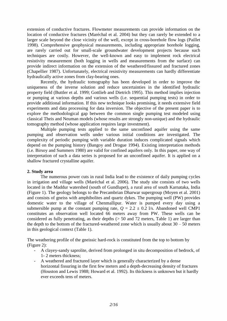
2. Study area

The numerous power cuts in rural India lead to the existence of daily pumping cycles

in irrigation and village wells (Maréchal et al. 2006). The study site consists of two wells

located in the Maddur watershed (south of Gundlupet), a rural area of south Karnataka, India

(Figure 1). The geology belongs to the Precambrian Dharwar supergroup (Moyen et al. 2001)

and consists of gneiss with amphibolites and quartz dykes. The pumping well (PW) provides

domestic water to the village of Chenmallipur. Water is pumped every day using a

submersible pump at the constant pumping rate, Q = 2.2 ± 0.2 l/s. Abandoned well CMP1

constitutes an observation well located 66 meters away from PW. These wells can be

considered as fully penetrating, as their depths (> 50 and 72 meters, Table 1) are larger than

the depth to the bottom of the fractured-weathered zone which is usually about 30 – 50 meters

in this geological context (Table 1).

The weathering profile of the gneissic hard-rock is constituted from the top to bottom by

(Figure 2):

- A clayey-sandy saprolite, derived from prolonged in situ decomposition of bedrock, of

1- 2 meters thickness;

- A weathered and fractured layer which is generally characterized by a dense

horizontal fissuring in the first few meters and a depth-decreasing density of fractures

(Houston and Lewis 1988; Howard et al. 1992). Its thickness is unknown but it hardly

ever exceeds tens of meters.

3/16

- The fresh basement which is permeable only where tectonic fractures are present. At

the catchment scale, this layer is generally considered as impermeable and of very low

porosity (Maréchal et al. 2004).

The water table fluctuates between 3 and 25 meters depth, thus only within the fractured

layer. It is therefore not restricted by any confining layer above it. The aquifer is a priori

unconfined and bounded below by the fresh basement (aquiclude). The saturated thickness is

not known.

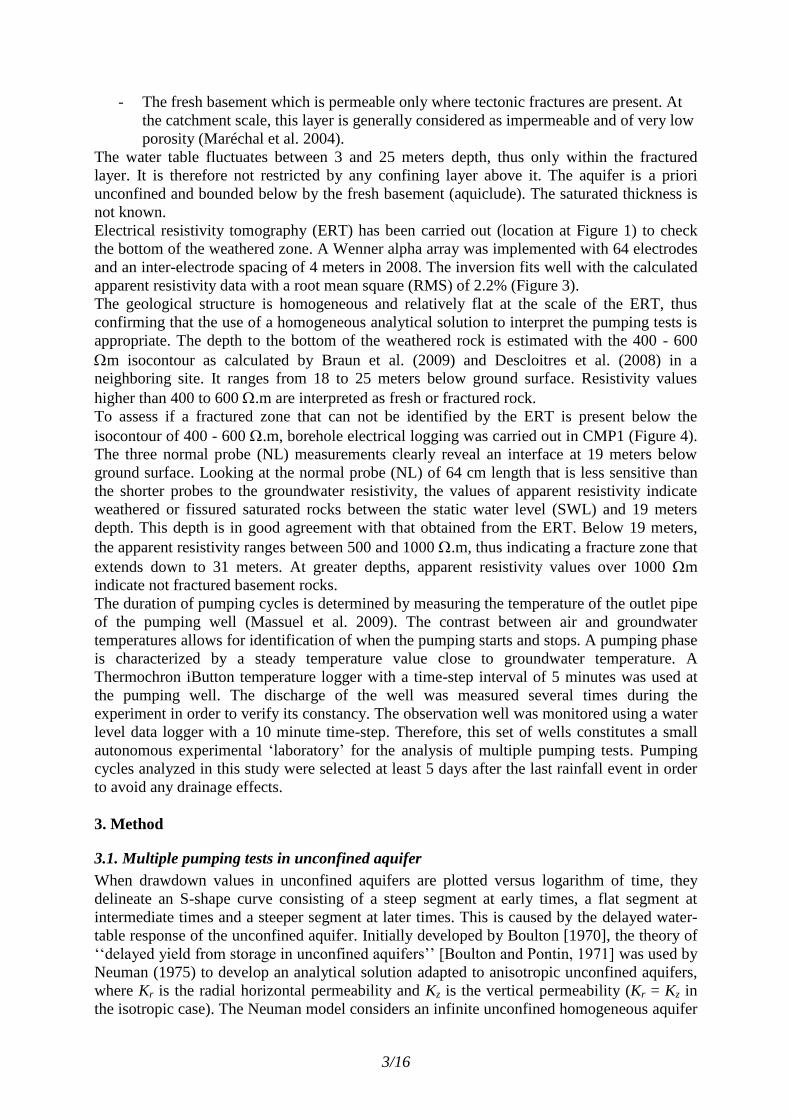
Electrical resistivity tomography (ERT) has been carried out (location at Figure 1) to check

the bottom of the weathered zone. A Wenner alpha array was implemented with 64 electrodes

and an inter-electrode spacing of 4 meters in 2008. The inversion fits well with the calculated

apparent resistivity data with a root mean square (RMS) of 2.2% (Figure 3).

The geological structure is homogeneous and relatively flat at the scale of the ERT, thus

confirming that the use of a homogeneous analytical solution to interpret the pumping tests is

appropriate. The depth to the bottom of the weathered rock is estimated with the 400 - 600

m isocontour as calculated by Braun et al. (2009) and Descloitres et al. (2008) in a

neighboring site. It ranges from 18 to 25 meters below ground surface. Resistivity values

higher than 400 to 600 .m are interpreted as fresh or fractured rock.

To assess if a fractured zone that can not be identified by the ERT is present below the

isocontour of 400 - 600 .m, borehole electrical logging was carried out in CMP1 (Figure 4).

The three normal probe (NL) measurements clearly reveal an interface at 19 meters below

ground surface. Looking at the normal probe (NL) of 64 cm length that is less sensitive than

the shorter probes to the groundwater resistivity, the values of apparent resistivity indicate

weathered or fissured saturated rocks between the static water level (SWL) and 19 meters

depth. This depth is in good agreement with that obtained from the ERT. Below 19 meters,

the apparent resistivity ranges between 500 and 1000 .m, thus indicating a fracture zone that

extends down to 31 meters. At greater depths, apparent resistivity values over 1000 m

indicate not fractured basement rocks.

The duration of pumping cycles is determined by measuring the temperature of the outlet pipe

of the pumping well (Massuel et al. 2009). The contrast between air and groundwater

temperatures allows for identification of when the pumping starts and stops. A pumping phase

is characterized by a steady temperature value close to groundwater temperature. A

Thermochron iButton temperature logger with a time-step interval of 5 minutes was used at

the pumping well. The discharge of the well was measured several times during the

experiment in order to verify its constancy. The observation well was monitored using a water

level data logger with a 10 minute time-step. Therefore, this set of wells constitutes a small

autonomous experimental ‘laboratory’ for the analysis of multiple pumping tests. Pumping

cycles analyzed in this study were selected at least 5 days after the last rainfall event in order

to avoid any drainage effects.

3. Method

3.1. Multiple pumping tests in unconfined aquifer

When drawdown values in unconfined aquifers are plotted versus logarithm of time, they

delineate an S-shape curve consisting of a steep segment at early times, a flat segment at

intermediate times and a steeper segment at later times. This is caused by the delayed water-

table response of the unconfined aquifer. Initially developed by Boulton [1970], the theory of

‘‘delayed yield from storage in unconfined aquifers’’ [Boulton and Pontin, 1971] was used by

Neuman (1975) to develop an analytical solution adapted to anisotropic unconfined aquifers,

where Kr is the radial horizontal permeability and Kz is the vertical permeability (Kr = Kz in

the isotropic case). The Neuman model considers an infinite unconfined homogeneous aquifer

4/16

with an initial saturated thickness b. When a complete well is pumped at a constant discharge

rate Q, one part of the water comes from elastic storage in the aquifer and the other from

gravitational drainage at the free surface (specific yield). The Neuman solution, plotted on

type curves, provides reduced drawdowns sD in an observation well located at a radial

distance r from the pumping well, Q

TssD

4 as a function of (a) reduced time 2Sr

TttS

for a series of ‘‘type A’’ curves (Neuman 1975) at early times; and (b) reduced time

2rS

Ttty

y for a series of ‘‘type B’’ curves at late times, where bKT

r (T is the

transmissivity of the aquifer), S is the storage coefficient, Sy is the specific yield, t is the time

since the start of pumping, and s is the drawdown. Therefore, matching a type A curve on

measured drawdown at early times leads to the estimate of S, while a type B curve at late

times leads to SY.

The storage coefficient matched on the type A curve can be written as

bbSSS

(1)

where 9.789 x 103 N/m

3 (γ is the specific weight of water at 20°C), is the

compressibility of the rock, 4.4x10-10

m2/N (β is the compressibility of water) and the

porosity of the rock.

In an unconfined aquifer, the transmissivity varies with the saturated thickness of the aquifer

b. Therefore, the interpretation of n pumping tests conducted with various saturated aquifer

thickness bi leads to n values of the transmissivity Ti = Kr bi, for i = 1, 2, …n. The

interpretation of multiple pumping tests precisely relies on the analysis of the relationship

between Kr bi and bi (Figure 5).

Let us consider a homogeneous and isotropic unconfined aquifer with a maximum saturated

thickness equal to bmax (corresponding to a minimum depth to water table dmin) measured after

a long recharge period (Figure 5a); the transmissivity at that time is equal to Kr bmax. During

the dry season, the water table declines and the transmissivity decreases to Kr bmin along with

the saturated thickness from bmax to bmin. A series of pumping tests conducted at various dates

during this period leads to a transmissivity ranging from Kr dmax to Kr dmin. The n plots of

estimated transmissivity according to the initial water-table depth should align along a straight

line with a slope inversely equal to the horizontal hydraulic conductivity Kr of the aquifer

(Figure 5b). The intercept of this straight line with the ordinates axis corresponds to the depth

d0 for which Kr b = 0, corresponding to the bottom of the aquifer.

Multiple pumping tests carried out on the same borewell are rare, costly and difficult to

implement. However pumping cycles induced by irrigation or drinking water supply wells can

be easily monitored using automatic water level recorders installed in close observation wells.

These intermittent pumping tests constitute an interesting and low-cost alternative technique

to conducting multiple pumping tests. The multiple pumping tests method can then be applied

in any region of the world with significant seasonal water table fluctuations (due to seasonal

rainfall during monsoon for example) and relatively short water pumping cycles.

3.2. Drawdown correction

Under daily pumping cycles, the short duration of the recovery phase does not allow

the system to recover to a static state before the next pumping phase. Therefore, the effect of

previous pumping phases on the drawdown should be taken into account. Two methods have

been tested for that purpose. The first method consists of interpreting several pumping and

recovery phases using the superposition principle (Bangoy and Drogue 1994) in order to

5/16

minimize the effect of non static initial conditions. However, increasing the duration of the

interpretation window induces an increasing effect on the existing trends, i.e. depletion trend

during dry season or increasing trend during monsoon. This leads to an overestimate of the

transmissivity during the monsoon and to an underestimate during the dry season. Therefore,

an alternative technique has been applied. For each pumping phase, the measured drawdown

has been corrected from the previous recovery phase as illustrated in Figure 6. The correction

involves computing the drawdown with respect to the water level that would have been

measured if the pumping had not have taken place (real drawdown), and not with respect to

the initial water level (apparent drawdown). In order to reconstruct what would have been the

water level, the previous recovery is extrapolated using an observed reference recovery

(Figure 6). Then the real drawdown is computed, adding to the observed drawdown the

remaining recovery s(t) which increases from 0 (at the beginning of the pumping phase,

Figure 6) to smax (at the end):

)()()(' tststs (1)

where s(t) is the observed apparent drawdown and s’(t) is the real drawdown corrected from

the previous recovery phase. This technique is actually an application of the superposition

principle valid for linear systems, which is not the case for an unconfined aquifer. Therefore

the error introduced by this assumption on hydrodynamic parameters estimation should be

computed. Practically, this error arises from the drawdown correction s(t) (0 < s(t) < smax)

which contradicts the hypothesis of a constant aquifer thickness. Therefore the maximum

uncertainty on estimated

bK is

b

s

bK

sbK

bK

bK

r

r

r

r maxmax1

(2)

where

bKr

is the transmissivity estimated after drawdown correction and bKr

the

transmissivity that would have been obtained if no correction was necessary. The same

uncertainty smax has been applied to the initial water-table depth. However, pumping tests

occurring after a recovery phase longer than 24 hours were not corrected as the water level

reached its initial level: the uncertainty is nil for these cases. Uncertainties are represented by

errors bars in Figures 10 and 11.

4. Results

The water-table fluctuations at well CMP1 during the monitoring period (January

2007 to August 2008) are presented Figure 7. The analysis of water-level signal leads to the

identification of two components. The trends of high amplitude are linked to the sequence of

dry and rainy seasons caused by the monsoon regime. Water-level fluctuations of lower

amplitude (and higher frequency) are caused by short pumping cycles. The trend in water-

table depth (between 2 and 25 meters below the surface) lends itself to being regarded as the

initial water levels of short pumping cycles. This is precisely the needed condition for the

application of the multiple pumping tests method described in this paper: existence of short

duration pumping cycles on an aquifer with seasonal high amplitude water-table fluctuations.

Consequently, each pumping cycle (identified by a serial number at Figure 7) can be

interpreted as an individual short duration pumping test with varying initial conditions.

4.1 Correction of the measured drawdown

The reference recovery scenario used for correcting the recorded drawdown is the 19

hours-long recovery observed between 19th and 20th August 2008. This reference was chosen

as it is the longest recovery recorded during the observation period and because it is located at

6/16

an average water-table depth. The recovery correction was independently applied to each

pumping test according to the duration of the previous pumping phase. Comparison between

several pumping tests (a, b, c, d and e, see Figure 8 for the dates) with close initial water

levels and different previous recovery phases shows that the corrected drawdowns are very

similar (Figure 8). The difference compared with uncorrected apparent drawdown is about 22

%. The coefficient of variation CV of the corrected drawdown has been computed at every

time step t as the ratio:

)('),('),('),('),('

)('),('),('),('),(')(

tststststs

tstststststCV

edcba

edcba

(3)

with the standard deviation and the average of corrected drawdown s’ during

pumping tests a, b, c, d and e at time t. CV tends to quickly decrease and becomes inferior to

10 % at early times (> 2 500 s, Figure 8). This shows that the effects of previous recovery

phases have been successfully corrected. It also suggests a very good repeatability of pumping

cycle results.

4.2 Interpretation of the corrected drawdown

The drawdown derivatives (diagnostic plot) of four pumping cycles and one recovery with

variable initial conditions are compared in Figure 9.

The equation used to calculate the drawdown derivative at the point of interest, i, is (Bourdet

et al. 1989):

21

1

2

2

2

1

1''

'

XX

XX

sX

X

s

dX

ds

i

(4)

where 1= point before i, 2 = point after, X is time function (ln t), and s’ is the corrected

drawdown. Noise effects are reduced by choosing the points 1 and 2 where the derivative is

calculated sufficiently distant from point i.

Figure 9 does not show the U-shape curve typical of delayed yield response of the unconfined

aquifer. This is due to the relative short duration of the pumping cycles and the quite long

distance between observation and pumping wells. In Fig 9 the general trend is a stabilization

of the derivative, corresponding to the early-times type A curve of the Neuman model.

One can also observe that the deeper the initial water level, the higher the derivative plateau

(Figure 9). This shows a decrease of the transmissivity with the water-table decline since

bKr

can directly be estimated from the derivative plateau (Chow 1952):

bK

Q

t

s

r4)ln(

'

(6)

Drawdown matches successfully the type A curves of the Neuman model for early times as

suggested by the diagnostic plot. The results of the interpretation of n = 24 pumping phases

between January 2007 and August 2008 for CMP1 are given at Erreur ! Source du renvoi

introuvable..

7/16

5. Discussion

5.1. Hydraulic conductivity and aquifer thickness

Within the investigated range of water-level depths (3.45 < di < 20.63 m), the

calculated transmissivity Ti = Kr bi (for i = 1 to 24) reasonably matches a linear relationship

with the initial depth to water level di (Figure 10). The deeper initial water level gives the

lower value of transmissivity. The observed linear relationship suggests that the horizontal

hydraulic conductivity Kr is constant with depth. Hydraulic conductivity Kr can be calculated

as the inverse slope of the fitted line as suggested earlier in Figure 5b. One linear regression is

calculated (Figure 10): the inverse slope of the linear regression is Kr = 3. 4.1

7.01

x 10

-6 m/s

(correlation coefficient R = 0.83). This value is similar to other results obtained for the Indian

Shield from slug tests (K = 4.4 x 10-6

m/s, Maréchal et al. 2004) and pumping tests (K = 1 x

10-5

m/s, Maréchal et al. 2004). The extrapolation of this linear relationship for Kr b = 0

provides the depth at which b = 0, that is the depth to the bottom of the aquifer d0 = 26.9 ± 4.5

m (Figure 10).

5.2. Specific storage

No clear relationship appears between calculated storage iS

bS and the water-table depth

(Figure 11). However, the obtained values range from 1.4 x 10-4

to 3.6 x 10-4

and are close to

the mean storage value obtained for the Indian Shield for granite (4.8 x 10-4

, Maréchal et al.

2004). Assuming 02.0 (Maréchal et al. 2006) in Eq. (1), 910

m

2/N (ranging from 10

-8

to 10-10

for fractured rock according to Kruseman and Ridder (1990)) and 20b m, one

obtains S = 2 x 10-4

which is very close to the values obtained using the Neuman model on

drawdown curves of short duration pumping tests. It is clear that the short duration pumping

tests do not lead to the estimate of specific yield but rather to the estimate of elastic storage.

Longer duration pumping tests are needed to determine the specific yield Sy of the aquifer

using the delayed yield approach (Neuman 1975).

The lack of linear relationship between storage and water-table depth suggests that the

specific storage is not homogeneous in this aquifer. As a consequence, the hydraulic

diffusivity (T/S) is not constant as well.

5.3. Comparison with geophysical data

Geophysical measurements suggest that the rock is weathered and highly fractured down to

19 meters below ground surface, and then the rock is moderately fractured down to 31 meters

deep. This result is in good agreement with the depth to the bottom of the aquifer obtained

from the pumping test analysis (d0 = 26.9 ± 4.5 m). It suggests that the hydraulically active

part of the aquifer is only located in the shallow weathered and densely fractured zones of the

crystalline basement (Maréchal 2009). This result also confirms other findings obtained in

crystalline aquifers from Africa (Chilton and Foster 1995; Houston and Lewis 1988; Taylor

and Howard 2000), the United States (Davis and Turk 1964) and India (Dewandel et al. 2006;

Maréchal et al. 2004).

6. Conclusion

Multiple pumping tests carried out on the same unconfined aquifer under various initial

conditions (initial water level) allow characterization of various responses of the system.

Interpretation of short-duration pumping phases shows that the transmissivity decreases

linearly with the increase of water-table depth. The extrapolation of this linear relation allows

for estimation of the aquifer thickness. The main advantage of this method is that it provides

8/16

the thickness of the really hydraulically active part of the aquifer. For the analyzed data set,

the obtained thickness is consistent with the local thickness of weathered fractured rocks

estimated using geophysical methods.

The main limitation of this method is that it requires high amplitude seasonal water-level

fluctuations. This method can be applied to other types of unconfined aquifer, for example,

aquifers present in sedimentary rocks. The use of longer pumping cycles would allow for

estimation of the total set of hydrodynamic parameters, including specific yield and the

permeability anisotropy ratio of the unconfined aquifer.

Acknowledgments

The Maddur Basin study is part of the ORE-BVET project (Observatoire de Recherche en

Environnement – Bassin Versant Expérimentaux Tropicaux). Apart from specific support

from the French Institute of Research for Development (IRD), the Embassy of France in India

and the Indian Institute of Science, our project benefited from funding from IRD and

INSU/CNRS (Institut National des Sciences de l’Univers / Centre National de la Recherche

Scientifique) through the French programmes ECCO-PNRH (Ecosphère Continentale:

Processus et Modélisation – Programme National Recherche Hydrologique) and EC2CO

(Ecosphère Continentale et Côtière). It is been funded by IFCPAR (Indo-French Center for

the Promotion of Advanced Research W-3000) and supported by ANR (National Research

Agency, France) under VMCS Programme No ANR-08-VULN-010-03/SHIVA. The

multidisciplinary research carried out on the Maddur watershed began in 2005 under the

control of the IISc/IRD laboratory IFCWS (Indo-French Cell for Water Sciences). The

authors warmly thank M. Sekhar, S. Subramanian and J.J. Braun for their support. The

contribution of Associate Editor Nadim Copty and Thomas Graf was highly appreciated.

References

Bangoy, L.M. and Drogue, C., 1994. Analysis of intermittent pumping tests in fissured fractal

aquifers: theory and applications. Journal of Hydrology, 158(1-2): 47-59.

Birsoy, Y.K. and Summers, W.K., 1980. Determination of Aquifer Parameters from Step

Tests and Intermittent Pumping Data. Ground Water, 18(2): 137-146.

Boulton, N. S. (1970), Analysis of data from pumping tests in unconfined anisotropic

aquifers, Journal of Hydrology, 10, 369–378.

Boulton, N. S., and J. M. A. Pontin (1971), An extended theory of delayed yield from storage

applied to pumping tests in unconfined anisotropic aquifers, Journal of Hydrology, 14,

53–65.

Bourdet, D., Ayoub, J.A. and Pirard, Y.M., 1989. Use of pressure derivative in well-test

interpretation. SPE Formation Evaluation, 4(2): 293-302.

Braun, J.J., Descloitres, M., Riotte, J., Fleury, S., Barbiero, L., Boeglin, J.L., Violette, A.,

Lacarce, E., Ruiz, L., Sekhar, M., Kumar, M.S.M., Subramanian, S. and Dupree, B.,

2009. Regolith mass balance inferred from combined mineralogical, geochemical and

geophysical studies: Mule Hole gneissic watershed, South India. Geochimica Et

Cosmochimica Acta, 73(4): 935-961.

Butler, J.J., Jr., McElwee, C.D. and Bohling, G.C., 1999. Pumping tests in networks of

multilevel sampling wells: Motivation and Method. Water Resources Research,

35(11): 3553-3560.

Chapellier, D., 1987. Diagraphies appliquées à l'hydrologie [Wells logging applied to

hydrology]. Lavoisier, Paris.

Chilton, P.J. and Foster, S.S.D., 1995. Hydrogeological characteristics and water-supply

potential of basement aquifers in Tropical Africa. Hydrogeology Journal, 3(1): 3-49.

9/16

Chow, V.T., 1952. On the determination of transmissibility and storage coefficients from

pumping test data. Trans Am Geophys Union, 33: 397-404.

Davis, S.N. and Turk, L.J., 1964. Optimum depth of wells in crystalline rocks. Groundwater,

2(2): 6-11.

Descloitres, M., Ruiz, L., Sekhar, M., Legchenko, A., Braun, J.J., Mohan Kumar, M.S. and

Subramanian, S., 2008. Characterization of seasonal local recharge using electrical

resistivity tomography and magnetic resonance sounding. Hydrological Processes,

22(3): 384-394.

Dewandel, B., Lachassagne, P., Wyns, R., Marechal, J.C. and Krishnamurthy, N.S., 2006. A

generalized 3-D geological and hydrogeological conceptual model of granite aquifers

controlled by single or multiphase weathering. Journal of Hydrology, 330(1-2): 260-

284.

Gottlieb, J. and Dietrich, P., 1995. Identification of the permeability distribution in soil by

hydraulic tomography. Inverse Problem, 11: 353-360.

Houston, J.F.T. and Lewis, R.T., 1988. The Victoria Province Drought Relief Project, II.

Borehole Yield Relationships. Ground Water, 26(4): 418-426.

Howard, K.W.F., Hughes, M., Charlesworth, D.L. and Ngobi, G., 1992. Hydrogeologic

Evaluation Of Fracture Permeability In Crystalline Basement Aquifers Of Uganda.

Hydrogeology Journal, 1(1): 55-65.

Kruseman, G.P. and Ridder, N.A., 1990. Analysis and evaluation of pumping test data. ILRI

Publication., 377 pp.

Maréchal, J.C., 2009. Editor’s message: the sunk cost fallacy of deep drilling. Hydrogeology

Journal, 18: 287-289, doi: 10.1007/s10040-009-0515-2.

Maréchal, J.C., Dewandel, B., Galeazzi, L., Bournet, G. and Ahmed, S., 2006. Combined

estimation of specific yield and natural recharge in a semi-arid groundwater basin with

irrigated agriculture. Journal of Hydrology, 329(1-2): 281-293.

Maréchal, J.C., Dewandel, B. and Subrahmanyam, K., 2004. Use of hydraulic tests at

different scales to characterize fracture network properties in the weathered-fractured

layer of a hard rock aquifer. Water Resources Research, 40(11).

Massuel, S., Perrin, J., Wajid, M., Mascre, C. and Dewandel, B., 2009. A Simple, Low-Cost

Method to Monitor Duration of Ground Water Pumping. Ground Water, 47(1): 141-

145.

Mayo, A.L., Morris, T.H., Peltier, S., Petersen, E.C., Payne, K., Holman, L.S., Tingey, D.,

Fogel, T., Black, B.J., Gibbs, T.D. (2003) Active and inactive groundwater flow

systems: evidence from a stratified, mountainous terrain. GSA Bull 115(12):1456–

1472

Moyen, J.F., Martin, H. and Jayananda, M., 2001. Multi- element geochemical modeling of

crust–mantle interactions during late-Archean crustal growth: the Closepet Granite

(South India). Precambrian Research, 112: 87-105.

Neuman, S.P., 1975. Analysis of Pumping Test Data From Anisotropic Unconfined Aquifers

Considering Delayed Gravity Response. Water Resources Research, 11(2): 329-342.

Paillet, F.L., 1998. Flow modeling and permeability estimation using borehole flow logs in

heterogeneous fractured formations. Water Resources Research, 34(5): 997-1010.

Taylor, R. and Howard, K., 2000. A tectono-geomorphic model of the hydrogeology of

deeply weathered crystalline rock: Evidence from Uganda. Hydrogeology Journal,

8(3): 279-294.

Theis, C.V. 1935. The relationship between the lowering of the piezometric surface and the

rate and duration of discharge of a well using groundwater storage. Eos Trans. AGU,

16, 519.

10/16

Figures

Figure 1: Location of the multiple pumping tests experimental site and the electrical

resistivity tomography (ERT) profile in Maddur watershed

Figure 2: Hydrogeological section of the pumping site (d0: depth to the bottom of the aquifer)

11/16

Figure 3: Electrical resistivity tomography (ERT) results

Figure 4: Electrical logging (CMP1, NP16, NP32 and NP64 are the lengths in cm of the used

probe)

12/16

Figure 5: (a) Unconfined aquifer with variable initial conditions of saturated thickness bi (b)

linear decrease of transmissivity with depth to water table; di is the depth to water

table

Figure 6: Example of a drawdown corrected with respect to the recovery effect

13/16

Figure 7: Water-table depth fluctuations at CMP1 during the monitoring period (analyzed

pumping cycles are numbered according to Table 2).

Figure 8: Corrected drawdown at CMP1 well during five pumping tests (PT) between 5th July

and 21st August 2008, with similar initial conditions (initial water-level depth d

ranging from 10 to 14 m)

14/16

Figure 9: Drawdown derivative of several pumping cycles starting with variable initial water-

table depths

Figure 10: Transmissivity obtained from multiple pumping tests at CMP1 as a function of

initial water-table depth

15/16

Figure 11: Storage coefficient obtained from multiple pumping tests at CMP1 as a function of

initial water-table depth

16/16

Tables

Table 1: Characteristics of monitored wells

Well Type Diameter

(m)

Depth

(m)

Distance to

PW (m)

Monitoring

device

PW Pumping

well

0.165 > 50 - Thermochron iButton

CMP1 Observation

well

0.165 72 66 Water level data logger

Table 2: Results of the interpretation of n = 24 pumping cycles at CMP1 using the Neuman model. i is the

pumping cycle number (see Figure 7). Ti and Si respectively transmissivity and storage coefficient

calculated from ith

pumping cycle.

i

Date

Initial water-

table depth di

(m)

Ti

(10-5

m²/s)

Si

(10-4

)

1 27/01/2007 10.14 4.3 2.1

2 26/05/2007 15.12 2.3 1.6

3 10/06/2007 20.63 2.9 1.5

4 12/06/2007 17.17 2.6 1.6

5 19/06/2007 21.23 2.8 1.4

6 21/06/2007 19.49 2.3 1.4

7 23/06/2007 16.73 2.3 1.5

8 29/06/2007 19.63 3.4 1.7

9 03/07/2007 18.60 3.7 1.9

10 05/07/2007 13.33 4.1 1.8

11 12/08/2007 8.35 4.9 2.0

12 25/08/2007 7.57 5.6 2.0

13 05/09/2007 7.35 4.2 1.4

14 10/09/2007 6.78 5.4 1.7

15 19/09/2007 3.58 6.9 1.9

16 22/09/2007 3.45 6.9 2.1

17 29/09/2007 3.40 5.9 1.7

18 05/07/2008 13.02 5.4 2.7

19 07/07/2008 13.71 5.2 2.7

20 19/07/2008 13.72 5.4 2.6

21 25/07/2008 16.08 4.5 3.6

22 09/08/2008 11.25 5.4 3.0

23 19/08/2008 9.93 5.9 2.6

24 21/08/2008 10.15 5.4 2.8

Average 12.52 4.5 2.1

Standard deviation 5.5 1.4 0.06

Coefficient of variation 0.44 0.32 0.29