Estimating and modelling relative survival using SAS

Paul Dickman

October 18, 2004

Contents

1 Quick start 2

2 Estimating relative survival 2

3 Overview of the approach to estimating relative survival in SAS 3

3.1 Contents of the ZIP archive . . . . . . . . . . . . . . . . . . . . . . . . . . . . . . . 4

3.2 The patient data file (colon.sas7bdat) . . . . . . . . . . . . . . . . . . . . . . . . 4

3.3 The population mortality file (popmort.sas7bdat) . . . . . . . . . . . . . . . . . . 5

4 Illustration of the code for estimating survival (survival.sas) 6

4.1 Checking the estimates using PROC LIFETEST . . . . . . . . . . . . . . . . . . . 12

4.2 Standard error of the observed survival proportion . . . . . . . . . . . . . . . . . . 13

4.3 Standard error of the relative survival ratio . . . . . . . . . . . . . . . . . . . . . . 13

4.4 Confidence intervals for observed and relative survival . . . . . . . . . . . . . . . . 13

4.5 Tabular and graphical presentation of survival estimates . . . . . . . . . . . . . . . 14

4.6 Variables contained in the output data sets GROUPED and INDIVID . . . . . . . 15

5 Modelling relative survival using SAS 16

5.1 Description of the model . . . . . . . . . . . . . . . . . . . . . . . . . . . . . . . . . 16

5.2 Esteve et al. full likelihood approach . . . . . . . . . . . . . . . . . . . . . . . . . . 17

5.3 Poisson regression approach . . . . . . . . . . . . . . . . . . . . . . . . . . . . . . . 18

5.4 Hakulinen–Tenkanen approach . . . . . . . . . . . . . . . . . . . . . . . . . . . . . 19

6 Estimating and modelling relative survival in SAS using period analysis 20

6.1 Overview of my approach to period analysis in SAS . . . . . . . . . . . . . . . . . 20

6.2 Estimating survival by transforming the hazard . . . . . . . . . . . . . . . . . . . . 20

6.3 An example . . . . . . . . . . . . . . . . . . . . . . . . . . . . . . . . . . . . . . . . 21

7 The Finnish Cancer Registry 23

References 24

1

1 Quick start

This document describes SAS code (version 7 or higher) for estimating and modelling relativesurvival. A sample data set containing information on colon carcinoma diagnosed in Finland isprovided. All required data and SAS files can be downloaded in a ZIP archive from:

http://www.pauldickman.com/rsmodel/sas colon.zip

If the files are extracted to the directory c:\rsmodel\sas_colon\ then the code should run withoutrequiring alteration. The code provided will reproduce the estimates reported in Table I of thepaper by Dickman et al. [1]. Two input data files are provided; colon.sas7bdat contains thecancer patient data and popmort.sas7bdat contains data on expected probabilities of death forthe Finnish general population.

Running the SAS code in survival.sas will produce life table estimates of relative survival strat-ified by sex, age, and calendar period of diagnosis. In addition, two output data sets are created(one containing grouped data and one containing individual patient data) which are used as inputdata sets for modelling. The SAS code in models.sas estimates a relative survival regressionmodel using several different approaches (described in Dickman et al. [1]).

In general, two data files are required in order to estimate relative survival; a file containingindividual-level data on the patients (see section 3.2) and a file containing expected probabilitiesof death for a comparable general population (see section 3.3). To estimate and model relativesurvival using other data it will almost certainly be necessary to modify the code to allow fordifferences in, for example, variable names and formats. Constructing your data set in a similarfashion to the example data sets (e.g., using identical variable names) is probably the easiest wayto get started.

2 Estimating relative survival

The relative survival ratio (RSR) is estimated using life table methods — the cumulative RSR isestimated at discrete points in the follow-up by taking the product of interval-specific estimatesover sub-intervals of the follow-up. For example, to estimate cumulative 10-year survival we mightestimate conditional survival (interval-specific survival) for each of 10 annual intervals and thenmultiply the interval-specific estimates to obtain the cumulative estimates. Following is an exampleof a resulting life table:

Life table estimates of patient survival

Males aged 0-44 diagnosed with colon carcinoma in Finland 1975-84

Interval- Interval- Interval-

specific Cumulative specific Cumulative specific Cumulative

observed observed expected expected relative relative

Int. N D W survival survival survival survival survival survival

0 - 1 75 4 0 0.94667 0.94667 0.99697 0.99697 0.94954 0.94954

1 - 2 71 8 0 0.88732 0.84000 0.99682 0.99381 0.89015 0.84524

2 - 3 63 1 1 0.98400 0.82656 0.99649 0.99032 0.98747 0.83464

3 - 4 61 3 0 0.95082 0.78591 0.99625 0.98660 0.95440 0.79658

4 - 5 58 3 0 0.94828 0.74526 0.99601 0.98266 0.95208 0.75841

5 - 6 55 2 0 0.96364 0.71816 0.99562 0.97836 0.96787 0.73404

6 - 7 53 0 0 1.00000 0.71816 0.99532 0.97378 1.00470 0.73749

7 - 8 53 0 0 1.00000 0.71816 0.99491 0.96882 1.00512 0.74127

8 - 9 53 1 0 0.98113 0.70461 0.99453 0.96352 0.98653 0.73128

9 - 10 52 2 0 0.96154 0.67751 0.99418 0.95792 0.96717 0.70727

2

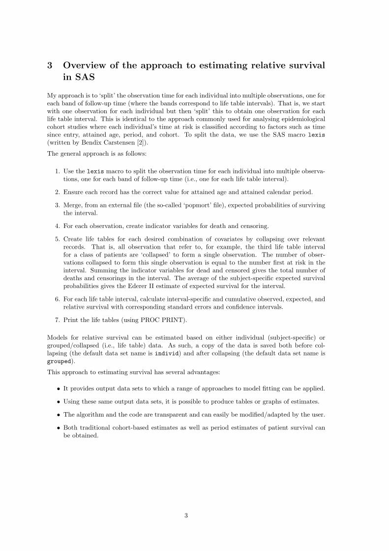
3 Overview of the approach to estimating relative survivalin SAS

My approach is to ‘split’ the observation time for each individual into multiple observations, one foreach band of follow-up time (where the bands correspond to life table intervals). That is, we startwith one observation for each individual but then ‘split’ this to obtain one observation for eachlife table interval. This is identical to the approach commonly used for analysing epidemiologicalcohort studies where each individual’s time at risk is classified according to factors such as timesince entry, attained age, period, and cohort. To split the data, we use the SAS macro lexis(written by Bendix Carstensen [2]).

The general approach is as follows:

1. Use the lexis macro to split the observation time for each individual into multiple observa-tions, one for each band of follow-up time (i.e., one for each life table interval).

2. Ensure each record has the correct value for attained age and attained calendar period.

3. Merge, from an external file (the so-called ‘popmort’ file), expected probabilities of survivingthe interval.

4. For each observation, create indicator variables for death and censoring.

5. Create life tables for each desired combination of covariates by collapsing over relevantrecords. That is, all observation that refer to, for example, the third life table intervalfor a class of patients are ‘collapsed’ to form a single observation. The number of obser-vations collapsed to form this single observation is equal to the number first at risk in theinterval. Summing the indicator variables for dead and censored gives the total number ofdeaths and censorings in the interval. The average of the subject-specific expected survivalprobabilities gives the Ederer II estimate of expected survival for the interval.

6. For each life table interval, calculate interval-specific and cumulative observed, expected, andrelative survival with corresponding standard errors and confidence intervals.

7. Print the life tables (using PROC PRINT).

Models for relative survival can be estimated based on either individual (subject-specific) orgrouped/collapsed (i.e., life table) data. As such, a copy of the data is saved both before col-lapsing (the default data set name is individ) and after collapsing (the default data set name isgrouped).

This approach to estimating survival has several advantages:

• It provides output data sets to which a range of approaches to model fitting can be applied.

• Using these same output data sets, it is possible to produce tables or graphs of estimates.

• The algorithm and the code are transparent and can easily be modified/adapted by the user.

• Both traditional cohort-based estimates as well as period estimates of patient survival canbe obtained.

3

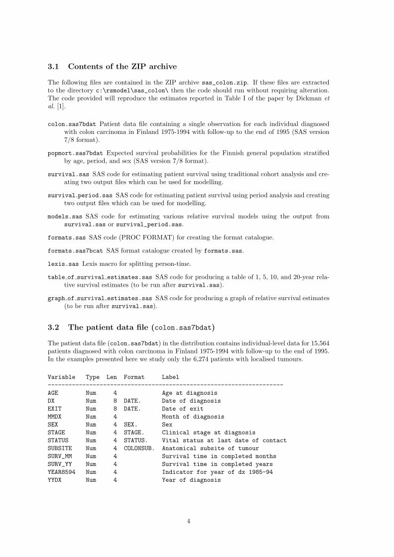
3.1 Contents of the ZIP archive

The following files are contained in the ZIP archive sas_colon.zip. If these files are extractedto the directory c:\rsmodel\sas_colon\ then the code should run without requiring alteration.The code provided will reproduce the estimates reported in Table I of the paper by Dickman etal. [1].

colon.sas7bdat Patient data file containing a single observation for each individual diagnosedwith colon carcinoma in Finland 1975-1994 with follow-up to the end of 1995 (SAS version7/8 format).

popmort.sas7bdat Expected survival probabilities for the Finnish general population stratifiedby age, period, and sex (SAS version 7/8 format).

survival.sas SAS code for estimating patient survival using traditional cohort analysis and cre-ating two output files which can be used for modelling.

survival period.sas SAS code for estimating patient survival using period analysis and creatingtwo output files which can be used for modelling.

models.sas SAS code for estimating various relative survival models using the output fromsurvival.sas or survival_period.sas.

formats.sas SAS code (PROC FORMAT) for creating the format catalogue.

formats.sas7bcat SAS format catalogue created by formats.sas.

lexis.sas Lexis macro for splitting person-time.

table of survival estimates.sas SAS code for producing a table of 1, 5, 10, and 20-year rela-tive survival estimates (to be run after survival.sas).

graph of survival estimates.sas SAS code for producing a graph of relative survival estimates(to be run after survival.sas).

3.2 The patient data file (colon.sas7bdat)

The patient data file (colon.sas7bdat) in the distribution contains individual-level data for 15,564patients diagnosed with colon carcinoma in Finland 1975-1994 with follow-up to the end of 1995.In the examples presented here we study only the 6,274 patients with localised tumours.

Variable Type Len Format Label--------------------------------------------------------------------AGE Num 4 Age at diagnosisDX Num 8 DATE. Date of diagnosisEXIT Num 8 DATE. Date of exitMMDX Num 4 Month of diagnosisSEX Num 4 SEX. SexSTAGE Num 4 STAGE. Clinical stage at diagnosisSTATUS Num 4 STATUS. Vital status at last date of contactSUBSITE Num 4 COLONSUB. Anatomical subsite of tumourSURV_MM Num 4 Survival time in completed monthsSURV_YY Num 4 Survival time in completed yearsYEAR8594 Num 4 Indicator for year of dx 1985-94YYDX Num 4 Year of diagnosis

4

In general, a file containing information on individuals diagnosed with cancer is required and mustcontain, at a minimum, the following information:

• Survival time (time at risk). In the examples from Finland survival time has been calculatedin advance although it is possible to specify the date of diagnosis and date of exit (seesection 4.0.2 on page 8).

• Indicator for vital status (dead/alive). Information on cause of death is not required.

• Variables upon which expected survival depends – typically age, sex, and period (as in theFinnish example) but can also include, for example, race, region/country of residence, orsocial class.

3.3 The population mortality file (popmort.sas7bdat)

The population mortality file (popmort.sas7bdat) contains expected survival probabilities (PROB)for the Finnish general population stratified by age, calendar year, and sex for the years 1951 to2000. Although the popmort file contains expected probabilities for each year, they were calculatedby the central statical office (Statistics Finland) for 5-year intervals so are identical, for example,for all years from 1951–1955.

An extract of the first 20 observations in the file is shown below.

SEX _YEAR _AGE PROB

1 1951 0 0.964291 1951 1 0.996391 1951 2 0.997831 1951 3 0.998421 1951 4 0.998821 1951 5 0.998931 1951 6 0.999131 1951 7 0.999051 1951 8 0.999201 1951 9 0.999311 1951 10 0.999401 1951 11 0.999391 1951 12 0.999201 1951 13 0.999251 1951 14 0.999141 1951 15 0.999131 1951 16 0.998971 1951 17 0.998821 1951 18 0.998351 1951 19 0.99836

In general, this file should be stratified by all variables upon which expected survival depends –typically age, sex, and period (as in the Finnish example) but can also include, for example, race,region/country of residence, or social class.

Survival is often estimated for subgroups defined by year of diagnosis or age at diagnosis. Whenestimating expected survival it is the age and year at time of follow-up (rather than at the time ofdiagnosis) that are important. That is, our data file will contain variables for both age at diagnosisand attained age (age at the time of follow-ups). I have adopted the convention of prefixing variablenames with an underscore when they are updated with follow-up, for example, the variable agecontains age at diagnosis and _age contains attained age.

5

4 Illustration of the code for estimating survival (survival.sas)

The approach is implemented as SAS code, rather than as a SAS macro, in order to make it moretransparent and easier to customize. The main parameters are, however, defined as macro variablesat the top of the file. For example, we first define the two input data files and specify filenamesfor the two output data files.

/* Population mortality file */%let popmort=colon.popmort ;

/* Patient data file */%let patdata=colon.colon ;

/* Output data file containing individual records */%let individ=colon.individ ;

/* Output data file containing collapsed data */%let grouped=colon.grouped ;

The macro variable vars stores the variables over which the life tables are stratified. The examplebelow results in a lifetable being estimated for each combination of sex, yydx (year of diagnosis),and age (at diagnosis). A single life table is estimated for every combination of each value of thesevariables. Formats can be used to group metric variables into categories. For example, the variableage contains age in completed years and a format is specified to group this into categories.

%let vars = sex yydx age;%let formats = sex sex. age age. yydx yydx. ;

The formats are defined in formats.sas and stored in the permanent format library colon.formats.The FMTSEARCH option is used (near the top of the code) to define the search path for formats.

The next step is a data step where housekeeping on the patient data file is performed. These taskscan, of course, be performed before running survival.sas but I have found it practical to includethem at this stage. For example, we exclude observations not eligible for the analysis (patientswith stage other than localised in the example) and drop variables not required (to reduce I/Otime).

/* Restrict to localised */if stage=1;

/* Create a unique ID for each observation */id+1;

/* Add 0.5 to all survival times */surv_mm = surv_mm + 0.5;

/* The lexis macro requires a variable containing the time at entry */entry=0;

/* an indicator variable for death due to any cause */if status in (1,2) then d=1;else d=0;

6

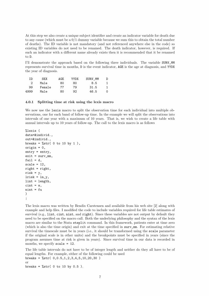
At this step we also create a unique subject identifier and create an indicator variable for death dueto any cause (which must be a 0/1 dummy variable because we sum this to obtain the total numberof deaths). The ID variable is not mandatory (and not referenced anywhere else in the code) soexisting ID variables do not need to be renamed. The death indicator, however, is required. Ifsuch an indicator with a different name already exists then it is recommended that it be renamedto D.

I’ll demonstrate the approach based on the following three individuals. The variable SURV_MMrepresents survival time in months, D is the event indicator, AGE is the age at diagnosis, and YYDXthe year of diagnosis.

ID SEX AGE YYDX SURV_MM D2 Male 80 80 8.5 1

99 Female 77 79 31.5 14999 Male 80 92 46.5 0

4.0.1 Splitting time at risk using the lexis macro

We now use the lexis macro to split the observation time for each individual into multiple ob-servations, one for each band of follow-up time. In the example we will split the observations intointervals of one year with a maximum of 10 years. That is, we wish to create a life table withannual intervals up to 10 years of follow-up. The call to the lexis macro is as follows

%lexis (data=&individ.,out=&individ.,breaks = %str( 0 to 10 by 1 ),origin = 0,entry = entry,exit = surv_mm,fail = d,scale = 12,right = right,risk = y,lrisk = ln_y,lint = length,cint = w,nint = fu);

The lexis macro was written by Bendix Carstensen and available from his web site [2] along withexample and help files. I modified the code to include variables required for life table estimates ofsurvival (e.g., lint, cint, nint, and right). Since these variables are not output by default theyneed to be specified on the macro call. Both the underlying philosophy and the syntax of the lexismacro are similar to the Stata stsplit command. In this framework, patients enter at time zero(which is also the time origin) and exit at the time specified in surv_mm. For estimating relativesurvival the timescale must be in years (i.e., it should be transformed using the scale parameterif the original scale is in other units) and the breakpoints must be specified in years (since theprogram assumes time at risk is given in years). Since survival time in our data is recorded inmonths, we specify scale = 12.

The life table intervals do not have to be of integer length and neither do they all have to be ofequal lengths. For example, either of the following could be usedbreaks = %str( 0,0.5,1,2,3,4,5,10,20,30 )orbreaks = %str( 0 to 10 by 0.5 ).

7

4.0.2 Specifying dates of entry and exit rather than the survival time

Rather than using the information on survival time in the variable surv_mm we can, alternatively,specify the dates of diagnosis and exit. That is, individuals enter the study at the date of diagnosis(which is the time origin) and exit at the date of death or censoring. The origin parameter isrequired since the time origin (i.e., time zero) occurs on a different date for each individual. Sincethe underlying time unit is now days we specify scale=365.25 to transform to years.

%lexis (data=&individ.,out=&individ.,breaks = %str( 0 to 10 by 1 ),origin = dx,entry = dx,exit = exit,fail = d,scale = 365.25,right = right,risk = y,lrisk = ln_y,lint = length,cint = w,nint = fu);

The Finnish cancer registry records only the month and year of diagnosis so the SAS date variablesdx and exit have been estimated from available information. In our example the resulting lifetables are identical for the two alternative methods of defining the time at risk although, in practice,it is possible to obtain slightly different results.

8

4.0.3 Updating age and period after splitting

Splitting the data results in the following

ID SEX AGE YYDX D W LEFT FU Y LENGTH

2 Male 80 80 1 0 0 1 0.70833 199 Female 77 79 0 0 0 1 1.00000 199 Female 77 79 0 0 1 2 1.00000 199 Female 77 79 1 0 2 3 0.62500 1

4999 Male 80 92 0 0 0 1 1.00000 14999 Male 80 92 0 0 1 2 1.00000 14999 Male 80 92 0 0 2 3 1.00000 14999 Male 80 92 0 1 3 4 0.87500 1

The variable LEFT holds the left breakpoint of the interval and Y the time at risk during the interval.LENGTH is the length of the interval (as distinct from the time at risk during the interval which isgiven by Y). The units for each of these variables is years.

Note that the variables AGE and YYDX represent the age and year at diagnosis, not the attained ageand year during the interval. We now want to create variables for attained age and calendar yearwhich are ‘updated’ for each observation for a single individual. These are the variables by whichwe will merge in the expected probabilities of death, so they must have the same names and sameformat as the variables indexing the POPMORT file (sex, _year, and _age in this example).

data &individ;set &individ;_age=floor(age+left);_year=floor(yydx+left);run;

This results in the following:

ID SEX AGE _AGE YYDX _YEAR D W FU Y LENGTH

2 Male 80 80 80 1980 1 0 1 0.70833 199 Female 77 77 79 1979 0 0 1 1.00000 199 Female 77 78 79 1980 0 0 2 1.00000 199 Female 77 79 79 1981 1 0 3 0.62500 1

4999 Male 80 80 92 1992 0 0 1 1.00000 14999 Male 80 81 92 1993 0 0 2 1.00000 14999 Male 80 82 92 1994 0 0 3 1.00000 14999 Male 80 83 92 1995 0 1 4 0.87500 1

Note that we must keep track of both age at diagnosis (which is used, for example, to stratify lifetables) and attained age (upon which the expected probability of death depends). Similarly, wemust keep track of both year of diagnosis and ‘attained’ year. My suggestion is that the variablenames for the updated quantities be prefixed with an underscore.

9

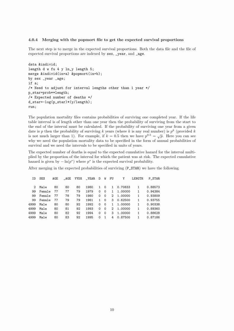
4.0.4 Merging with the popmort file to get the expected survival proportions

The next step is to merge in the expected survival proportions. Both the data file and the file ofexpected survival proportions are indexed by sex, _year, and _age.

data &individ;length d w fu 4 y ln_y length 5;merge &individ(in=a) &popmort(in=b);by sex _year _age;if a;/* Need to adjust for interval lengths other than 1 year */p_star=prob**length;/* Expected number of deaths */d_star=-log(p_star)*(y/length);run;

The population mortality files contains probabilities of surviving one completed year. If the lifetable interval is of length other than one year then the probability of surviving from the start tothe end of the interval must be calculated. If the probability of surviving one year from a givendate is p then the probability of surviving k years (where k is any real number) is pk (provided kis not much larger than 1). For example, if k = 0.5 then we have p0.5 =

√p. Here you can see

why we need the population mortality data to be specified in the form of annual probabilities ofsurvival and we need the intervals to be specified in units of years.

The expected number of deaths is equal to the expected cumulative hazard for the interval multi-plied by the proportion of the interval for which the patient was at risk. The expected cumulativehazard is given by − ln(p∗) where p∗ is the expected survival probability.

After merging in the expected probabilities of surviving (P_STAR) we have the following

ID SEX AGE _AGE YYDX _YEAR D W FU Y LENGTH P_STAR

2 Male 80 80 80 1980 1 0 1 0.70833 1 0.88573

99 Female 77 77 79 1979 0 0 1 1.00000 1 0.94384

99 Female 77 78 79 1980 0 0 2 1.00000 1 0.93809

99 Female 77 79 79 1981 1 0 3 0.62500 1 0.93755

4999 Male 80 80 92 1992 0 0 1 1.00000 1 0.90338

4999 Male 80 81 92 1993 0 0 2 1.00000 1 0.89360

4999 Male 80 82 92 1994 0 0 3 1.00000 1 0.88628

4999 Male 80 83 92 1995 0 1 4 0.87500 1 0.87186

10

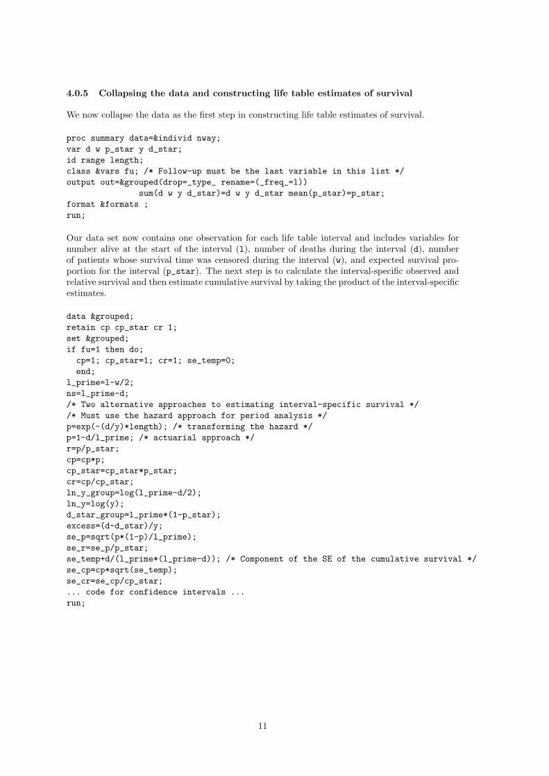
4.0.5 Collapsing the data and constructing life table estimates of survival

We now collapse the data as the first step in constructing life table estimates of survival.

proc summary data=&individ nway;var d w p_star y d_star;id range length;class &vars fu; /* Follow-up must be the last variable in this list */output out=&grouped(drop=_type_ rename=(_freq_=l))

sum(d w y d_star)=d w y d_star mean(p_star)=p_star;format &formats ;run;

Our data set now contains one observation for each life table interval and includes variables fornumber alive at the start of the interval (l), number of deaths during the interval (d), numberof patients whose survival time was censored during the interval (w), and expected survival pro-portion for the interval (p_star). The next step is to calculate the interval-specific observed andrelative survival and then estimate cumulative survival by taking the product of the interval-specificestimates.

data &grouped;retain cp cp_star cr 1;set &grouped;if fu=1 then do;

cp=1; cp_star=1; cr=1; se_temp=0;end;

l_prime=l-w/2;ns=l_prime-d;/* Two alternative approaches to estimating interval-specific survival *//* Must use the hazard approach for period analysis */p=exp(-(d/y)*length); /* transforming the hazard */p=1-d/l_prime; /* actuarial approach */r=p/p_star;cp=cp*p;cp_star=cp_star*p_star;cr=cp/cp_star;ln_y_group=log(l_prime-d/2);ln_y=log(y);d_star_group=l_prime*(1-p_star);excess=(d-d_star)/y;se_p=sqrt(p*(1-p)/l_prime);se_r=se_p/p_star;se_temp+d/(l_prime*(l_prime-d)); /* Component of the SE of the cumulative survival */se_cp=cp*sqrt(se_temp);se_cr=se_cp/cp_star;... code for confidence intervals ...run;

11

The final step is to print the estimates (using PROC PRINT) in the form of life tables. A list ofvariables available is provided in Section 4.6 (page 15).

Colon carcinoma diagnosed in Finland 1975-1994 (follow-up to 1995)

Life table estimates of patient survival

The Ederer II method is used to estimate expected survival

Sex=Male Year of diagnosis=1975-84 Age at diagnosis=0-44

Interval- Interval- Interval-

specific Cumulative specific Cumulative specific Cumulative

observed observed expected expected relative relative

Int. N D W survival survival survival survival survival survival

0 - 1 75 4 0 0.94667 0.94667 0.99697 0.99697 0.94954 0.94954

1 - 2 71 8 0 0.88732 0.84000 0.99682 0.99381 0.89015 0.84524

2 - 3 63 1 1 0.98400 0.82656 0.99649 0.99032 0.98747 0.83464

3 - 4 61 3 0 0.95082 0.78591 0.99625 0.98660 0.95440 0.79658

4 - 5 58 3 0 0.94828 0.74526 0.99601 0.98266 0.95208 0.75841

5 - 6 55 2 0 0.96364 0.71816 0.99562 0.97836 0.96787 0.73404

6 - 7 53 0 0 1.00000 0.71816 0.99532 0.97378 1.00470 0.73749

7 - 8 53 0 0 1.00000 0.71816 0.99491 0.96882 1.00512 0.74127

8 - 9 53 1 0 0.98113 0.70461 0.99453 0.96352 0.98653 0.73128

9 - 10 52 2 0 0.96154 0.67751 0.99418 0.95792 0.96717 0.70727

4.1 Checking the estimates using PROC LIFETEST

The estimates of observed survival obtained using my approach should be identical to the estimatesobtained from PROC LIFETEST - it is recommended that such a test be performed. For example,the life estimates shown in the previous table can be obtained with the following code:

proc lifetest data=colon.colon(where=(stage=1)) method=act width=12;time surv_mm*status(0,4);strata sex yydx age;format sex sex. age age. yydx yydx.;run;

Stratum 16: SEX = Male YYDX = 1975-84 AGE = 0-44

Conditional

Effective Conditional Probability

Interval Number Number Sample Probability Standard

[Lower, Upper) Failed Censored Size of Failure Error Survival

0 12 4 0 75.0 0.0533 0.0259 1.0000

12 24 8 0 71.0 0.1127 0.0375 0.9467

24 36 1 1 62.5 0.0160 0.0159 0.8400

36 48 3 0 61.0 0.0492 0.0277 0.8266

48 60 3 0 58.0 0.0517 0.0291 0.7859

60 72 2 0 55.0 0.0364 0.0252 0.7453

72 84 0 0 53.0 0 0 0.7182

84 96 0 0 53.0 0 0 0.7182

96 108 1 0 53.0 0.0189 0.0187 0.7182

108 120 2 0 52.0 0.0385 0.0267 0.7046

120 132 1 0 50.0 0.0200 0.0198 0.6775

Note how PROC LIFETEST presents the interval-specific failure (rather than survival) proportionand that the estimates of cumulative survival are presented for the start of each interval (i.e., theyare offset by one row compared to the way in which I present the estimates).

12

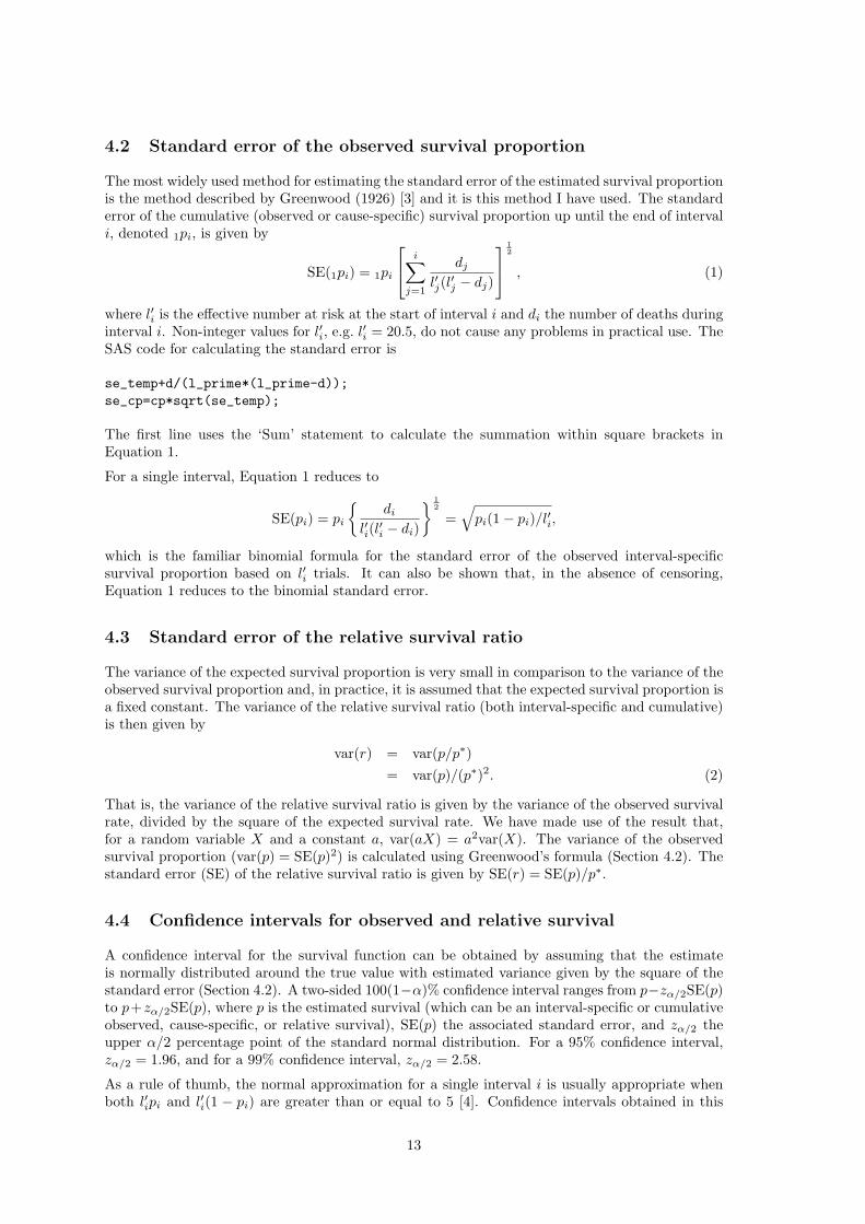
4.2 Standard error of the observed survival proportion

The most widely used method for estimating the standard error of the estimated survival proportionis the method described by Greenwood (1926) [3] and it is this method I have used. The standarderror of the cumulative (observed or cause-specific) survival proportion up until the end of intervali, denoted 1pi, is given by

SE(1pi) = 1pi

i∑

j=1

dj

l′j(l′j − dj)

12

, (1)

where l′i is the effective number at risk at the start of interval i and di the number of deaths duringinterval i. Non-integer values for l′i, e.g. l′i = 20.5, do not cause any problems in practical use. TheSAS code for calculating the standard error is

se_temp+d/(l_prime*(l_prime-d));se_cp=cp*sqrt(se_temp);

The first line uses the ‘Sum’ statement to calculate the summation within square brackets inEquation 1.

For a single interval, Equation 1 reduces to

SE(pi) = pi

{di

l′i(l′i − di)

} 12

=√

pi(1− pi)/l′i,

which is the familiar binomial formula for the standard error of the observed interval-specificsurvival proportion based on l′i trials. It can also be shown that, in the absence of censoring,Equation 1 reduces to the binomial standard error.

4.3 Standard error of the relative survival ratio

The variance of the expected survival proportion is very small in comparison to the variance of theobserved survival proportion and, in practice, it is assumed that the expected survival proportion isa fixed constant. The variance of the relative survival ratio (both interval-specific and cumulative)is then given by

var(r) = var(p/p∗)= var(p)/(p∗)2. (2)

That is, the variance of the relative survival ratio is given by the variance of the observed survivalrate, divided by the square of the expected survival rate. We have made use of the result that,for a random variable X and a constant a, var(aX) = a2var(X). The variance of the observedsurvival proportion (var(p) = SE(p)2) is calculated using Greenwood’s formula (Section 4.2). Thestandard error (SE) of the relative survival ratio is given by SE(r) = SE(p)/p∗.

4.4 Confidence intervals for observed and relative survival

A confidence interval for the survival function can be obtained by assuming that the estimateis normally distributed around the true value with estimated variance given by the square of thestandard error (Section 4.2). A two-sided 100(1−α)% confidence interval ranges from p−zα/2SE(p)to p+zα/2SE(p), where p is the estimated survival (which can be an interval-specific or cumulativeobserved, cause-specific, or relative survival), SE(p) the associated standard error, and zα/2 theupper α/2 percentage point of the standard normal distribution. For a 95% confidence interval,zα/2 = 1.96, and for a 99% confidence interval, zα/2 = 2.58.

As a rule of thumb, the normal approximation for a single interval i is usually appropriate whenboth l′ipi and l′i(1 − pi) are greater than or equal to 5 [4]. Confidence intervals obtained in this

13

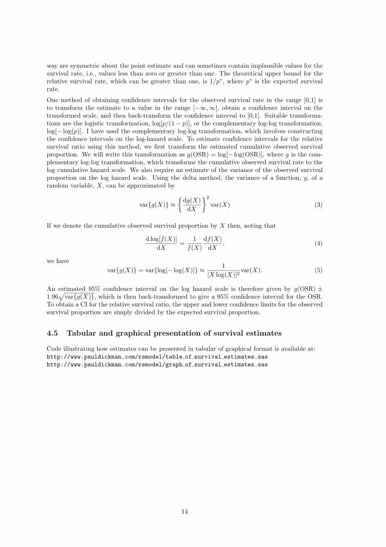
way are symmetric about the point estimate and can sometimes contain implausible values for thesurvival rate, i.e., values less than zero or greater than one. The theoretical upper bound for therelative survival rate, which can be greater than one, is 1/p∗, where p∗ is the expected survivalrate.

One method of obtaining confidence intervals for the observed survival rate in the range [0,1] isto transform the estimate to a value in the range [−∞,∞], obtain a confidence interval on thetransformed scale, and then back-transform the confidence interval to [0,1]. Suitable transforma-tions are the logistic transformation, log[p/(1− p)], or the complementary log-log transformation,log[− log(p)]. I have used the complementary log-log transformation, which involves constructingthe confidence intervals on the log-hazard scale. To estimate confidence intervals for the relativesurvival ratio using this method, we first transform the estimated cumulative observed survivalproportion. We will write this transformation as g(OSR) = log[− log(OSR)], where g is the com-plementary log-log transformation, which transforms the cumulative observed survival rate to thelog cumulative hazard scale. We also require an estimate of the variance of the observed survivalproportion on the log hazard scale. Using the delta method, the variance of a function, g, of arandom variable, X, can be approximated by

var{g(X)} ≈{

dg(X)dX

}2

var(X) (3)

If we denote the cumulative observed survival proportion by X then, noting that

d log[f(X)]dX

=1

f(X)df(X)

dX, (4)

we havevar{g(X)} = var{log[− log(X)]} ≈ 1

[X log(X)]2var(X). (5)

An estimated 95% confidence interval on the log hazard scale is therefore given by g(OSR) ±1.96

√var{g(X)}, which is then back-transformed to give a 95% confidence interval for the OSR.

To obtain a CI for the relative survival ratio, the upper and lower confidence limits for the observedsurvival proportion are simply divided by the expected survival proportion.

4.5 Tabular and graphical presentation of survival estimates

Code illustrating how estimates can be presented in tabular of graphical format is available at:http://www.pauldickman.com/rsmodel/table of survival estimates.sashttp://www.pauldickman.com/rsmodel/graph of survival estimates.sas

14

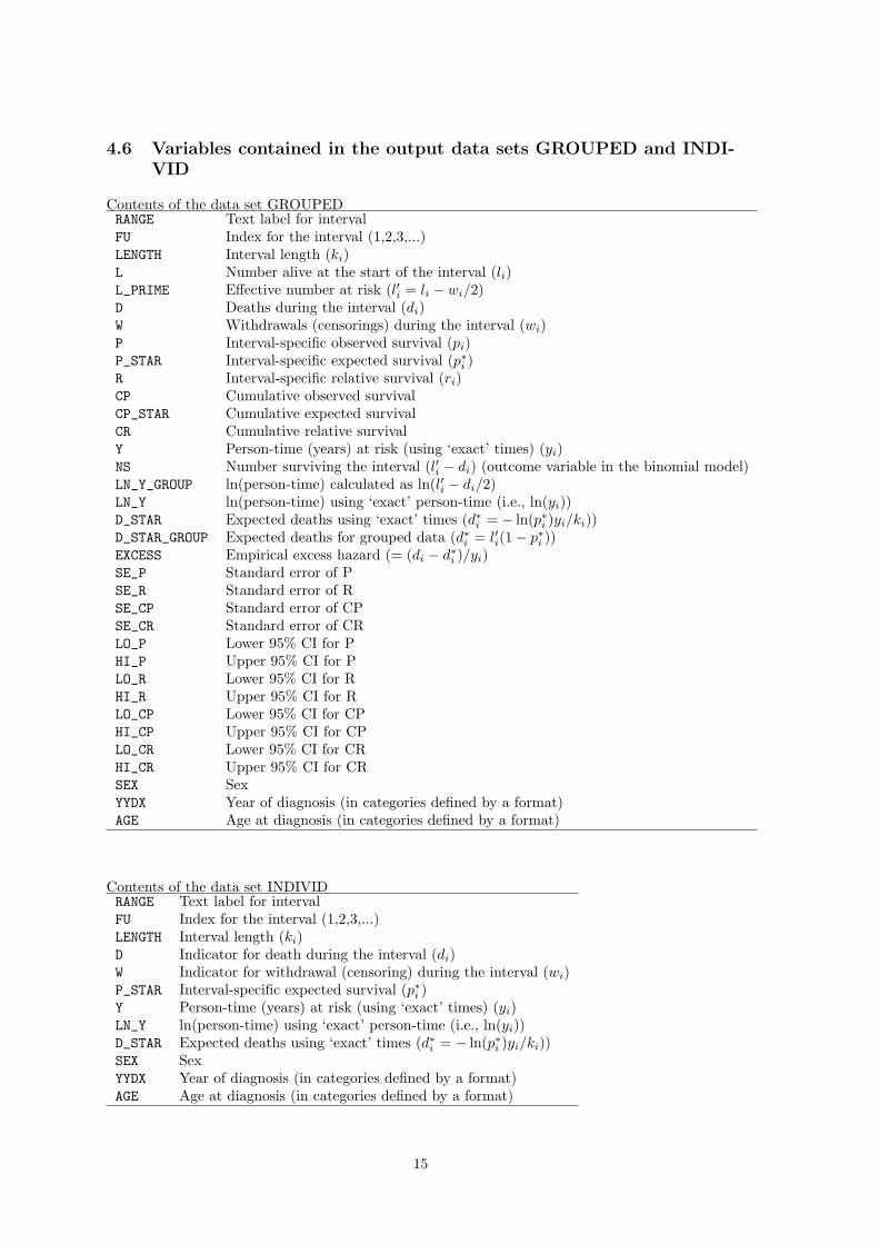
4.6 Variables contained in the output data sets GROUPED and INDI-VID

Contents of the data set GROUPEDRANGE Text label for intervalFU Index for the interval (1,2,3,...)LENGTH Interval length (ki)L Number alive at the start of the interval (li)L_PRIME Effective number at risk (l′i = li − wi/2)D Deaths during the interval (di)W Withdrawals (censorings) during the interval (wi)P Interval-specific observed survival (pi)P_STAR Interval-specific expected survival (p∗i )R Interval-specific relative survival (ri)CP Cumulative observed survivalCP_STAR Cumulative expected survivalCR Cumulative relative survivalY Person-time (years) at risk (using ‘exact’ times) (yi)NS Number surviving the interval (l′i − di) (outcome variable in the binomial model)LN_Y_GROUP ln(person-time) calculated as ln(l′i − di/2)LN_Y ln(person-time) using ‘exact’ person-time (i.e., ln(yi))D_STAR Expected deaths using ‘exact’ times (d∗i = − ln(p∗i )yi/ki))D_STAR_GROUP Expected deaths for grouped data (d∗i = l′i(1− p∗i ))EXCESS Empirical excess hazard (= (di − d∗i )/yi)SE_P Standard error of PSE_R Standard error of RSE_CP Standard error of CPSE_CR Standard error of CRLO_P Lower 95% CI for PHI_P Upper 95% CI for PLO_R Lower 95% CI for RHI_R Upper 95% CI for RLO_CP Lower 95% CI for CPHI_CP Upper 95% CI for CPLO_CR Lower 95% CI for CRHI_CR Upper 95% CI for CRSEX SexYYDX Year of diagnosis (in categories defined by a format)AGE Age at diagnosis (in categories defined by a format)

Contents of the data set INDIVIDRANGE Text label for intervalFU Index for the interval (1,2,3,...)LENGTH Interval length (ki)D Indicator for death during the interval (di)W Indicator for withdrawal (censoring) during the interval (wi)P_STAR Interval-specific expected survival (p∗i )Y Person-time (years) at risk (using ‘exact’ times) (yi)LN_Y ln(person-time) using ‘exact’ person-time (i.e., ln(yi))D_STAR Expected deaths using ‘exact’ times (d∗i = − ln(p∗i )yi/ki))SEX SexYYDX Year of diagnosis (in categories defined by a format)AGE Age at diagnosis (in categories defined by a format)

15

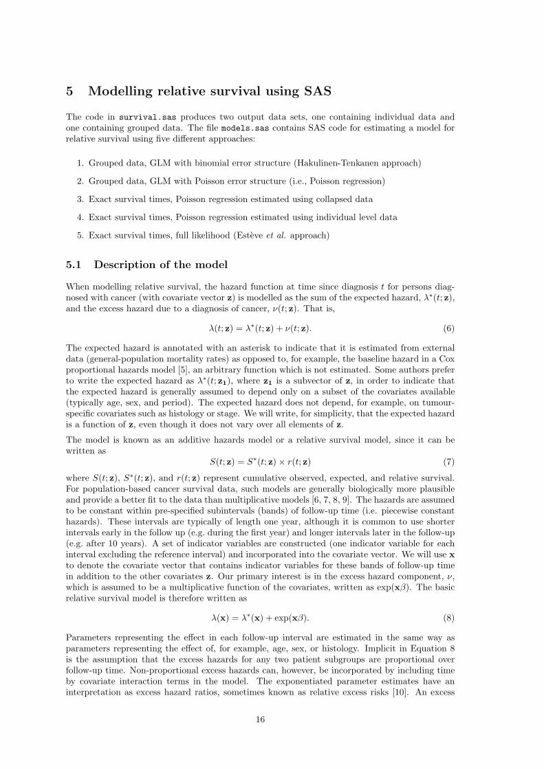
5 Modelling relative survival using SAS

The code in survival.sas produces two output data sets, one containing individual data andone containing grouped data. The file models.sas contains SAS code for estimating a model forrelative survival using five different approaches:

1. Grouped data, GLM with binomial error structure (Hakulinen-Tenkanen approach)

2. Grouped data, GLM with Poisson error structure (i.e., Poisson regression)

3. Exact survival times, Poisson regression estimated using collapsed data

4. Exact survival times, Poisson regression estimated using individual level data

5. Exact survival times, full likelihood (Esteve et al. approach)

5.1 Description of the model

When modelling relative survival, the hazard function at time since diagnosis t for persons diag-nosed with cancer (with covariate vector z) is modelled as the sum of the expected hazard, λ∗(t; z),and the excess hazard due to a diagnosis of cancer, ν(t; z). That is,

λ(t; z) = λ∗(t; z) + ν(t; z). (6)

The expected hazard is annotated with an asterisk to indicate that it is estimated from externaldata (general-population mortality rates) as opposed to, for example, the baseline hazard in a Coxproportional hazards model [5], an arbitrary function which is not estimated. Some authors preferto write the expected hazard as λ∗(t; z1), where z1 is a subvector of z, in order to indicate thatthe expected hazard is generally assumed to depend only on a subset of the covariates available(typically age, sex, and period). The expected hazard does not depend, for example, on tumour-specific covariates such as histology or stage. We will write, for simplicity, that the expected hazardis a function of z, even though it does not vary over all elements of z.

The model is known as an additive hazards model or a relative survival model, since it can bewritten as

S(t; z) = S∗(t; z)× r(t; z) (7)

where S(t; z), S∗(t; z), and r(t; z) represent cumulative observed, expected, and relative survival.For population-based cancer survival data, such models are generally biologically more plausibleand provide a better fit to the data than multiplicative models [6, 7, 8, 9]. The hazards are assumedto be constant within pre-specified subintervals (bands) of follow-up time (i.e. piecewise constanthazards). These intervals are typically of length one year, although it is common to use shorterintervals early in the follow up (e.g. during the first year) and longer intervals later in the follow-up(e.g. after 10 years). A set of indicator variables are constructed (one indicator variable for eachinterval excluding the reference interval) and incorporated into the covariate vector. We will use xto denote the covariate vector that contains indicator variables for these bands of follow-up timein addition to the other covariates z. Our primary interest is in the excess hazard component, ν,which is assumed to be a multiplicative function of the covariates, written as exp(xβ). The basicrelative survival model is therefore written as

λ(x) = λ∗(x) + exp(xβ). (8)

Parameters representing the effect in each follow-up interval are estimated in the same way asparameters representing the effect of, for example, age, sex, or histology. Implicit in Equation 8is the assumption that the excess hazards for any two patient subgroups are proportional overfollow-up time. Non-proportional excess hazards can, however, be incorporated by including timeby covariate interaction terms in the model. The exponentiated parameter estimates have aninterpretation as excess hazard ratios, sometimes known as relative excess risks [10]. An excess

16

hazard ratio of, for example, 1.5 for males compared to females implies that the excess hazardassociated with a diagnosis of cancer is 50% higher for males than females.

Various approaches to estimating the model, and their implementation in SAS, are described inthe following sections.

5.2 Esteve et al. full likelihood approach

Esteve et al. [8] described a method for estimating the model in Equation 8 directly from individual-level data using a full maximum likelihood approach. The likelihood function is

L =n∏

i=1

exp(−∫ ti

0

λ(s) ds)[λ(ti)]di , (9)

where ti is the survival time and di the failure indicator variable (1 if ti is the time of death; 0 ifthe survival time is censored at ti) for each of the i = 1, . . . , n individuals.

Writing the total hazard as the sum of the expected hazard and the excess hazard, the log-likelihoodfunction is

l(β) = −n∑

i=1

∫ ti

0

λ∗(s) ds−n∑

i=1

∫ ti

0

ν(s) ds +n∑

i=1

di ln[λ∗(ti) + ν(ti)]. (10)

Although the model is specified in continuous time it is assumed, as with all approaches describedhere, that the hazard is constant within pre-specified bands of time and the excess hazard ν(t) iswritten as exp(xβ). Estimation of the model is simplified if each observation is split into separateobservations for each band of follow-up. Rather than evaluating the log likelihood for each subjectand summing over subjects (the Esteve et al. approach) we evaluate the log-likelihood for eachsubject-band. The log likelihood function, expressed in terms of the J subject-band observations,is

l(β) =J∑

j=1

[dj ln[λ∗(xj) + exp(xjβ)]− yj exp(xjβ)] . (11)

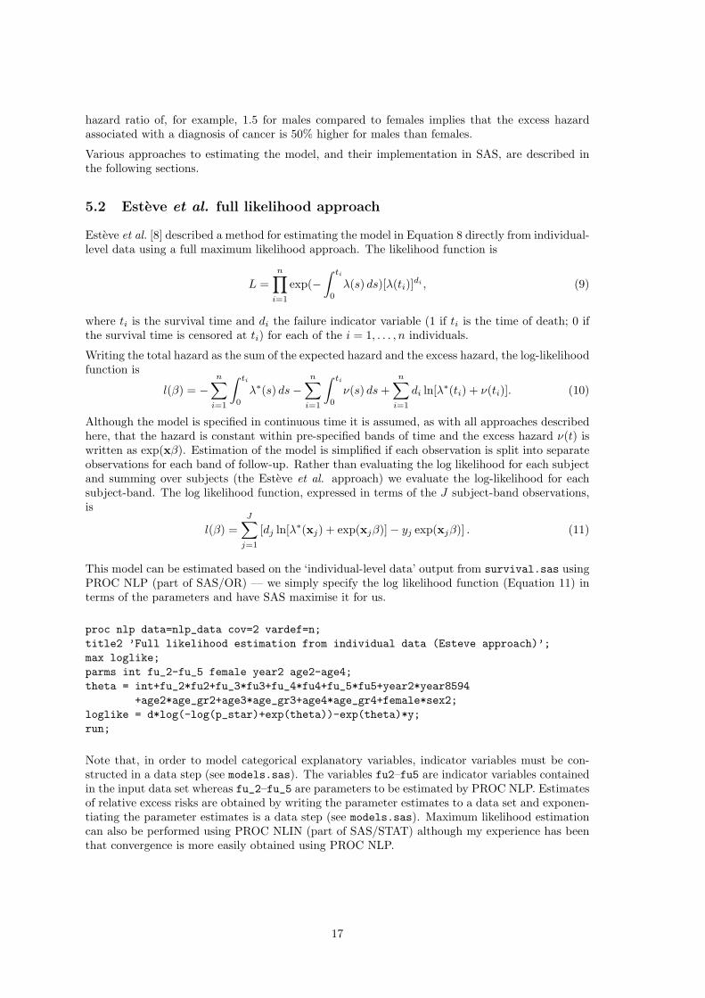
This model can be estimated based on the ‘individual-level data’ output from survival.sas usingPROC NLP (part of SAS/OR) — we simply specify the log likelihood function (Equation 11) interms of the parameters and have SAS maximise it for us.

proc nlp data=nlp_data cov=2 vardef=n;title2 ’Full likelihood estimation from individual data (Esteve approach)’;max loglike;parms int fu_2-fu_5 female year2 age2-age4;theta = int+fu_2*fu2+fu_3*fu3+fu_4*fu4+fu_5*fu5+year2*year8594

+age2*age_gr2+age3*age_gr3+age4*age_gr4+female*sex2;loglike = d*log(-log(p_star)+exp(theta))-exp(theta)*y;run;

Note that, in order to model categorical explanatory variables, indicator variables must be con-structed in a data step (see models.sas). The variables fu2–fu5 are indicator variables containedin the input data set whereas fu_2–fu_5 are parameters to be estimated by PROC NLP. Estimatesof relative excess risks are obtained by writing the parameter estimates to a data set and exponen-tiating the parameter estimates is a data step (see models.sas). Maximum likelihood estimationcan also be performed using PROC NLIN (part of SAS/STAT) although my experience has beenthat convergence is more easily obtained using PROC NLP.

17

5.3 Poisson regression approach

The relative survival model (Equation 8) assumes piecewise constant hazards which implies aPoisson process for the number of deaths in each interval; see Andersen et al. [11, pp. 409] orBreslow and Day [12, Section 4.2]. The log likelihood in Equation 11 is therefore identical to thelog-likelihood for grouped Poisson data with intensity λ∗(x) + exp(xβ) [12, pp. 185] except weomitted the term −yjλ

∗(xj) since it did not depend on β.

This implies that the relative survival model can be estimated in the framework of generalisedlinear models using a Poisson assumption for the observed number of deaths. If the model isestimated from subject-band observations the estimates will be identical to those obtained usingthe full likelihood approach (Section 5.2) since we maximise the same likelihood based on the samedata. We can also, however, estimate the model based on collapsed or grouped data, in which casethe estimates differ slightly.

We assume that the number of deaths, dj , for observation j can be described by a Poisson distri-bution, dj ∼ Poisson(µj) where µj = λjyj and yj is person-time at risk for the observation. Theobservations can represent either life table intervals (in which case there can be multiple deathsper observation), individual patients, or subject-bands (as in Section 5.2).

Equation 8 is then written asµj/yj = d∗j/yj + exp(xβ), (12)

which can be written asln(µj − d∗j ) = ln(yj) + xβ, (13)

where d∗j is the expected number of deaths (due to causes other than the cancer of interest andestimated from general population mortality rates). This implies a generalised linear model withoutcome dj , Poisson error structure, link ln(µj−d∗j ), and offset ln(yj). Such a model was suggestedby Berry (1983) [13] and is specified in PROC GENMOD as follows

proc genmod data=&grouped(where=(fu le 5)) order=formatted;title2 ’Poisson error model fitted to collapsed data’;title3 ’Main effects model (follow-up, sex, age, and dgnyear)’;fwdlink link = log(_MEAN_-d_star);invlink ilink= exp(_XBETA_)+d_star;class fu sex age yydx;model d = fu sex yydx age / error=poisson offset=ln_y type3;format fu fu. age age. yydx yydx.;run;

Estimates of relative excess risks are obtained by writing the parameter estimates to a data setand exponentiating the parameter estimates is a data step (see models.sas).

5.3.1 Estimation based on collapsed or grouped data

The model can be estimated directly from subject-band observations (in the data set &individ) orthe subject-band observations can be collapsed to give one observation for each covariate pattern(d, d∗, and y are summed within each covariate pattern) as in the data set &grouped. Estimating astandard Poisson regression model (with logarithmic link and offset ln(yj)) gives identical estimatesfor both individual and collapsed data. Estimating Equation 13 based on collapsed data, however,leads to slightly different estimates to those obtained from subject-band observations since d∗

varies within each covariate pattern (i.e. combination of follow-up interval, sex, period, age group,etc.). The model can also be estimated based on grouped data (information is available only onthe number of events in a time interval rather than exact times to event for each individual). Inthis case we can estimate the expected number of deaths as d∗i = l′i(1 − p∗i ) and the log person-time at risk as ln(l′i − di/2). These two quantities are stored in the variable D_STAR_GROUP) andLN_Y_GROUP in the GROUPED data set.

18

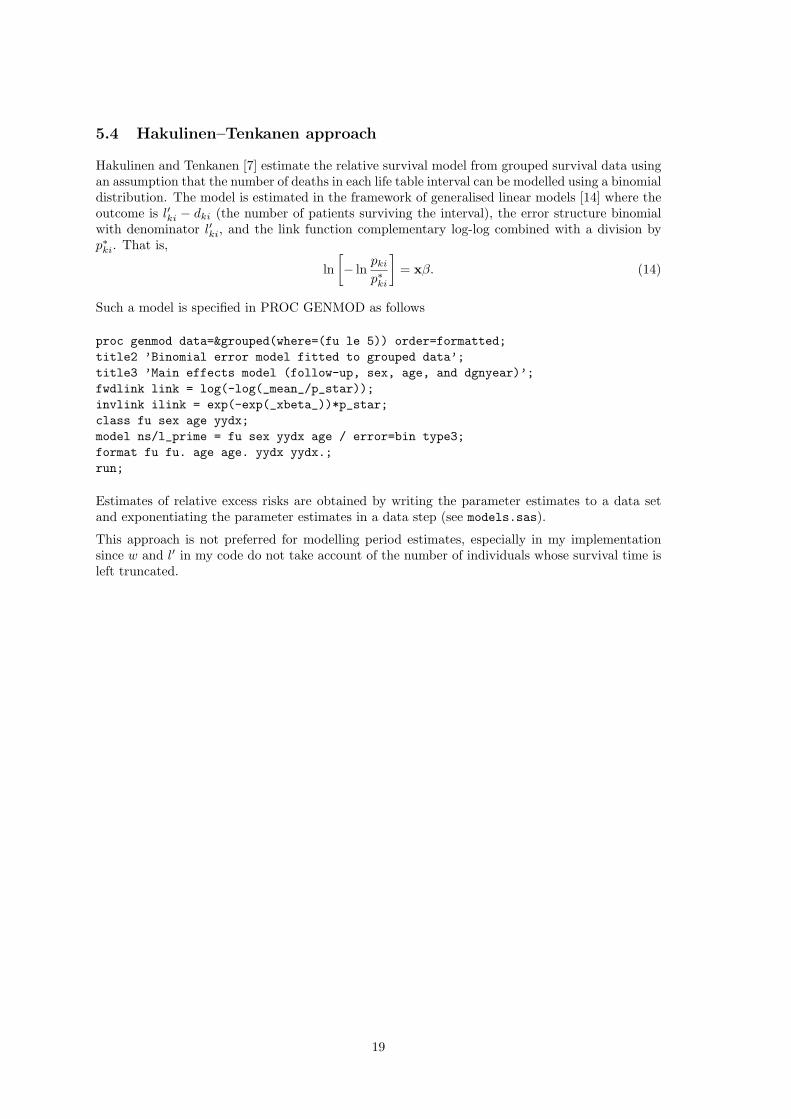
5.4 Hakulinen–Tenkanen approach

Hakulinen and Tenkanen [7] estimate the relative survival model from grouped survival data usingan assumption that the number of deaths in each life table interval can be modelled using a binomialdistribution. The model is estimated in the framework of generalised linear models [14] where theoutcome is l′ki − dki (the number of patients surviving the interval), the error structure binomialwith denominator l′ki, and the link function complementary log-log combined with a division byp∗ki. That is,

ln[− ln

pki

p∗ki

]= xβ. (14)

Such a model is specified in PROC GENMOD as follows

proc genmod data=&grouped(where=(fu le 5)) order=formatted;title2 ’Binomial error model fitted to grouped data’;title3 ’Main effects model (follow-up, sex, age, and dgnyear)’;fwdlink link = log(-log(_mean_/p_star));invlink ilink = exp(-exp(_xbeta_))*p_star;class fu sex age yydx;model ns/l_prime = fu sex yydx age / error=bin type3;format fu fu. age age. yydx yydx.;run;

Estimates of relative excess risks are obtained by writing the parameter estimates to a data setand exponentiating the parameter estimates in a data step (see models.sas).

This approach is not preferred for modelling period estimates, especially in my implementationsince w and l′ in my code do not take account of the number of individuals whose survival time isleft truncated.

19

6 Estimating and modelling relative survival in SAS usingperiod analysis

In 1996 Hermann Brenner [15, 16] suggested that lifetable estimates of patient survival could bemade using a period rather than the traditional cohort approach. Period analysis has since beenshown to provide more accurate predictions of newly diagnosed patients and is able to detecttemporal trends in patient survival sooner than the traditional cohort approach [17, 18, 19].

Professor Brenner and colleagues have produced SAS macros for estimating survival using periodanalysis which are available athttp://www.imbe.med.uni-erlangen.de/issan/SAS/period/period.htm

These macros can be used to estimate survival using either the cohort or the period approachand expected survival can be calculated using either the Ederer II or the Hakulinen method. Myapproach to estimating survival can also be used for period analysis and excess mortality can bemodelled in the same manner as with cohort analysis. I estimate expected survival using theEderer II method (the Hakulinen method is not implemented) although this is sufficient when theprimary interest is in modelling.

6.1 Overview of my approach to period analysis in SAS

There are two differences when using my approach for period analysis compared to cohort analysis.The first is that we use the lexis macro an additional time to restrict the time at risk to thecalendar window of interest. The second difference is that interval-specific observed survival isestimated by transforming the estimated hazard rate rather than by using the actuarial estimator.The approach is as follows:

1. Split the data by calendar time using the lexis macro so, for each individual, we retain onlythe time at risk during the calendar window of interest. For example, we might be interestedin the time at risk between 1 January 1994 and 31 December 1995. If an individual is not atrisk during the period of interest (e.g., they have died before the start of the window or arediagnosed after the window) then they do not contribute to the analysis. After this step ourdata set will consist of (at most) one observation per individual.

2. Split the resulting data by time since diagnosis in the usual manner. Each individual maycontribute more than one observation.

3. Collapse the data and estimate life tables in the usual manner. A slight difference from thecohort approach is that we estimate survival by transforming the cumulative hazard (ratherthan using the actuarial method).

6.2 Estimating survival by transforming the hazard

The standard actuarial estimator for the interval-specific observed survival for interval i is

pi = (1− di/l′i)

where di is the number if deaths in the interval and l′i = 1 − wi/2 is the ‘effective number atrisk’ (wi is the number censored during the interval). In period analysis survival times can be lefttruncated in addition to being right censored so fewer subjects are at risk for the full interval. Assuch, wi would need to represent the number of individuals whose survival time was left truncatedor right censored. However, it is possible that some survival times would be both left truncatedand right censored during the interval (and hence be, on average, at risk for only one quarter ofthe interval) so the estimator would need to be modified to account for this.

An alternative approach is to use the relationship that the survivor function is equal to the expo-nential of the negative of the cumulative hazard (S = exp(−Λ)). The cumulative hazard, Λ, is the

20

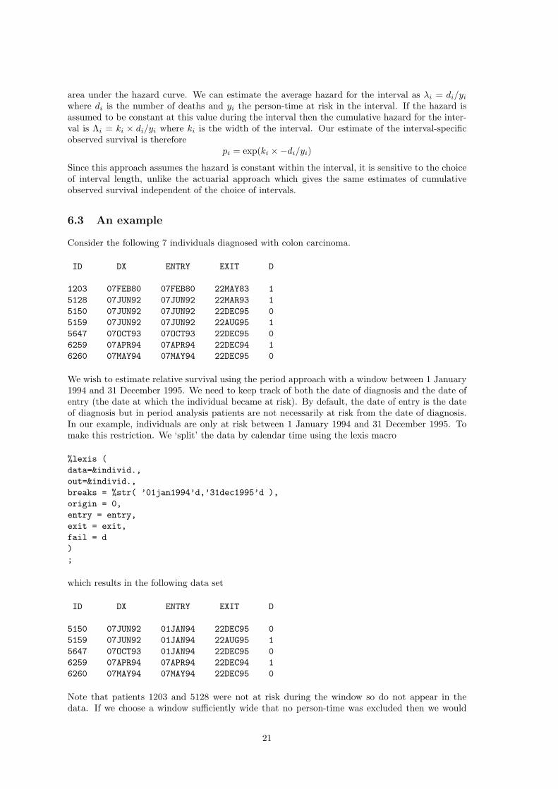
area under the hazard curve. We can estimate the average hazard for the interval as λi = di/yi

where di is the number of deaths and yi the person-time at risk in the interval. If the hazard isassumed to be constant at this value during the interval then the cumulative hazard for the inter-val is Λi = ki × di/yi where ki is the width of the interval. Our estimate of the interval-specificobserved survival is therefore

pi = exp(ki ×−di/yi)

Since this approach assumes the hazard is constant within the interval, it is sensitive to the choiceof interval length, unlike the actuarial approach which gives the same estimates of cumulativeobserved survival independent of the choice of intervals.

6.3 An example

Consider the following 7 individuals diagnosed with colon carcinoma.

ID DX ENTRY EXIT D

1203 07FEB80 07FEB80 22MAY83 15128 07JUN92 07JUN92 22MAR93 15150 07JUN92 07JUN92 22DEC95 05159 07JUN92 07JUN92 22AUG95 15647 07OCT93 07OCT93 22DEC95 06259 07APR94 07APR94 22DEC94 16260 07MAY94 07MAY94 22DEC95 0

We wish to estimate relative survival using the period approach with a window between 1 January1994 and 31 December 1995. We need to keep track of both the date of diagnosis and the date ofentry (the date at which the individual became at risk). By default, the date of entry is the dateof diagnosis but in period analysis patients are not necessarily at risk from the date of diagnosis.In our example, individuals are only at risk between 1 January 1994 and 31 December 1995. Tomake this restriction. We ‘split’ the data by calendar time using the lexis macro

%lexis (data=&individ.,out=&individ.,breaks = %str( ’01jan1994’d,’31dec1995’d ),origin = 0,entry = entry,exit = exit,fail = d);

which results in the following data set

ID DX ENTRY EXIT D

5150 07JUN92 01JAN94 22DEC95 05159 07JUN92 01JAN94 22AUG95 15647 07OCT93 01JAN94 22DEC95 06259 07APR94 07APR94 22DEC94 16260 07MAY94 07MAY94 22DEC95 0

Note that patients 1203 and 5128 were not at risk during the window so do not appear in thedata. If we choose a window sufficiently wide that no person-time was excluded then we would

21

obtain the usual cohort estimates. We need to keep track of both the date of diagnosis (dx) andthe date at which the person entered the risk set (entry). Note, for example, that patient 5150was diagnosed on 7 June 1992 but did not enter the risk set until 1 January 1994. At the timethis patient became ‘at risk’ he or she was in the 2nd year subsequent to diagnosis and will not,therefore, contribute to the survival estimate for the first life table interval.

We now split by time since diagnosis (in the same manner as when we estimate survival using thecohort approach).

%lexis (data=&individ.,out=&individ.,breaks = %str( 0 to 10 by 1 ),origin = dx,entry = entry,exit = exit,fail = d,scale = 365.25,right = right,risk = y,lrisk = ln_y,lint = length,cint = w,nint = fu);

The time origin is the date of diagnosis and each patient enters the risk set at the entry date (whichis not necessarily the same as the date of diagnosis as it was in cohort analysis). The resultingdata set is as follows:

ID LEFT FU DX ENTRY EXIT Y D

5150 1 2 07JUN92 01JAN94 07JUN94 0.43121 05150 2 3 07JUN92 07JUN94 07JUN95 1.00000 05150 3 4 07JUN92 07JUN95 22DEC95 0.54004 05159 1 2 07JUN92 01JAN94 07JUN94 0.43121 05159 2 3 07JUN92 07JUN94 07JUN95 1.00000 05159 3 4 07JUN92 07JUN95 22AUG95 0.20602 15647 0 1 07OCT93 01JAN94 07OCT94 0.76454 05647 1 2 07OCT93 07OCT94 07OCT95 1.00000 05647 2 3 07OCT93 07OCT95 22DEC95 0.20671 06259 0 1 07APR94 07APR94 22DEC94 0.70910 16260 0 1 07MAY94 07MAY94 07MAY95 1.00000 06260 1 2 07MAY94 07MAY95 22DEC95 0.62628 0

22

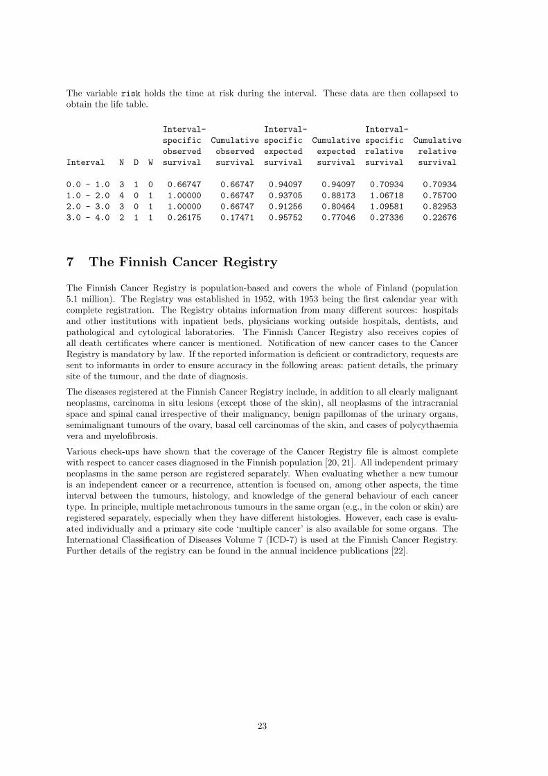
The variable risk holds the time at risk during the interval. These data are then collapsed toobtain the life table.

Interval- Interval- Interval-specific Cumulative specific Cumulative specific Cumulativeobserved observed expected expected relative relative

Interval N D W survival survival survival survival survival survival

0.0 - 1.0 3 1 0 0.66747 0.66747 0.94097 0.94097 0.70934 0.709341.0 - 2.0 4 0 1 1.00000 0.66747 0.93705 0.88173 1.06718 0.757002.0 - 3.0 3 0 1 1.00000 0.66747 0.91256 0.80464 1.09581 0.829533.0 - 4.0 2 1 1 0.26175 0.17471 0.95752 0.77046 0.27336 0.22676

7 The Finnish Cancer Registry

The Finnish Cancer Registry is population-based and covers the whole of Finland (population5.1 million). The Registry was established in 1952, with 1953 being the first calendar year withcomplete registration. The Registry obtains information from many different sources: hospitalsand other institutions with inpatient beds, physicians working outside hospitals, dentists, andpathological and cytological laboratories. The Finnish Cancer Registry also receives copies ofall death certificates where cancer is mentioned. Notification of new cancer cases to the CancerRegistry is mandatory by law. If the reported information is deficient or contradictory, requests aresent to informants in order to ensure accuracy in the following areas: patient details, the primarysite of the tumour, and the date of diagnosis.

The diseases registered at the Finnish Cancer Registry include, in addition to all clearly malignantneoplasms, carcinoma in situ lesions (except those of the skin), all neoplasms of the intracranialspace and spinal canal irrespective of their malignancy, benign papillomas of the urinary organs,semimalignant tumours of the ovary, basal cell carcinomas of the skin, and cases of polycythaemiavera and myelofibrosis.

Various check-ups have shown that the coverage of the Cancer Registry file is almost completewith respect to cancer cases diagnosed in the Finnish population [20, 21]. All independent primaryneoplasms in the same person are registered separately. When evaluating whether a new tumouris an independent cancer or a recurrence, attention is focused on, among other aspects, the timeinterval between the tumours, histology, and knowledge of the general behaviour of each cancertype. In principle, multiple metachronous tumours in the same organ (e.g., in the colon or skin) areregistered separately, especially when they have different histologies. However, each case is evalu-ated individually and a primary site code ‘multiple cancer’ is also available for some organs. TheInternational Classification of Diseases Volume 7 (ICD-7) is used at the Finnish Cancer Registry.Further details of the registry can be found in the annual incidence publications [22].

23

References

[1] Dickman PW, Sloggett A, Hills M, Hakulinen T. Regression models for relative survival.Statistics in Medicine 2004;23:51–64.

[2] Carstensen B. Lexis macro for splitting person-time in sas, 2004. http://www.biostat.ku.dk/∼bxc/Lexis/.

[3] Greenwood M. The Errors of Sampling of the Survivorship Table, vol. 33 of Reports on PublicHealth and Medical Subjects. London: Her Majesty’s Stationery Office, 1926.

[4] Altman DG. Practical Statistics for Medical Research. London: Chapman and Hall, 1991.

[5] Cox DR. Regression models and life tables (with discussion). Journal of the Royal StatisticalSociety Series B 1972;34:187–220.

[6] Buckley JD. Additive and multiplicative models for relative survival rates. Biometrics 1984;40:51–62.

[7] Hakulinen T, Tenkanen L. Regression analysis of relative survival rates. Applied Statistics1987;36:309–317.

[8] Esteve J, Benhamou E, Croasdale M, Raymond L. Relative survival and the estimation ofnet survival: Elements for further discussion. Statistics in Medicine 1990;9:529–538.

[9] Bolard P, Quantin C, Esteve J, Faivre J, Abrahamowicz M. Modelling time-dependent hazardratios in relative survival: Application to colon cancer. Journal of Clinical Epidemiology 2001;54:986–996.

[10] Suissa S. Relative excess risk: An alternative measure of comparitive risk. American Journalof Epidemiology 1999;150:279–282.

[11] Andersen PK, Borgan , Gill RD, Keiding N. Statistical Models Based on Counting Processes.Springer-Verlag, 1995.

[12] Breslow NE, Day NE. Statistical Methods in Cancer Research: Volume II - The Design andAnalysis of Cohort Studies. IARC Scientific Publications No. 82. Lyon: International Agencyfor Research on Cancer, 1987.

[13] Berry G. The analysis of mortality by the subject-years method. Biometrics 1983;39:173–184.

[14] McCullagh P, Nelder JA. Generalized Linear Models. London: Chapman and Hall, 2nd edn.,1989.

[15] Brenner H, Gefeller O. An alternative approach to monitoring cancer patient survival. Cancer1996;78:2004–2010.

[16] Brenner H, Gefeller O. Deriving more up-to-date estimates of long-term patient survival.Journal of Clinical Epidemiology 1997;50:211–216.

[17] Brenner H, Gefeller O, Stegmaier C, Ziegler H. More up-to-date monitoring of long-termsurvival rates by cancer registries: an empirical example. Methods Inf Med 2001;40:248–52.

[18] Brenner H, Hakulinen T. Up-to-date long-term survival curves of patients with cancer byperiod analysis. Journal of Clinical Oncology 2002;20:826–832.

[19] Brenner H, Gefeller O, Hakulinen T. Period analysis for ‘up-to-date’ cancer survival data:theory, empirical evaluation, computational realisation and applications. European Journal ofCancer 2004;40:326–35.

[20] Teppo L, Pukkala E, Lehtonen M. Data quality and quality control of a population-basedcancer registry. Experience in Finland. Acta Oncologica 1994;33:365–369.

24

[21] Hakulinen T. Health care system, cancer registration and follow-up of cancer patients inFinland. In: Berrino F, Sant M, Verdecchia A, Capocaccia R, Hakulinen T, Esteve J, eds.,Survival of Cancer Patients in Europe: The EUROCARE Study , IARC Scientific PublicationsNo. 132. Lyon: International Agency for Research on Cancer, 1995; 53–54.

[22] Finnish Cancer Registry. Cancer Incidence in Finland 1995 . Cancer Society of FinlandPublication No. 58. Helsinki: Cancer Society of Finland, 1997.

25